Measure, Probability, Quantum - Stellenbosch...
49
Measure, Probability, Quantum Kevin H. Knuth 1 and John Skilling 2 1. University at Albany (SUNY), USA 2. Maximum Entropy Data Consultants Ltd, Kenmare, Ireland 1
Transcript of Measure, Probability, Quantum - Stellenbosch...
Measure, Probability,Quantum
Kevin H. Knuth1 and John Skilling2
1. University at Albany (SUNY), USA2. Maximum Entropy Data Consultants Ltd, Kenmare, Ireland
1

A Question Posed
“Why is it that when I take two pencils and add one pencil, I always get three pencils?
And when I take two pennies and add one penny, I always get three pennies,
and so on with rocks and sticks and candy and monkeys and planets and stars.
Is this true by definition as in 2+1 defines 3? Or is it an experimental fact so that at some point in the distant past this observation needed to be verified again and again?”
- Kevin Knuth
2
A Question Posed
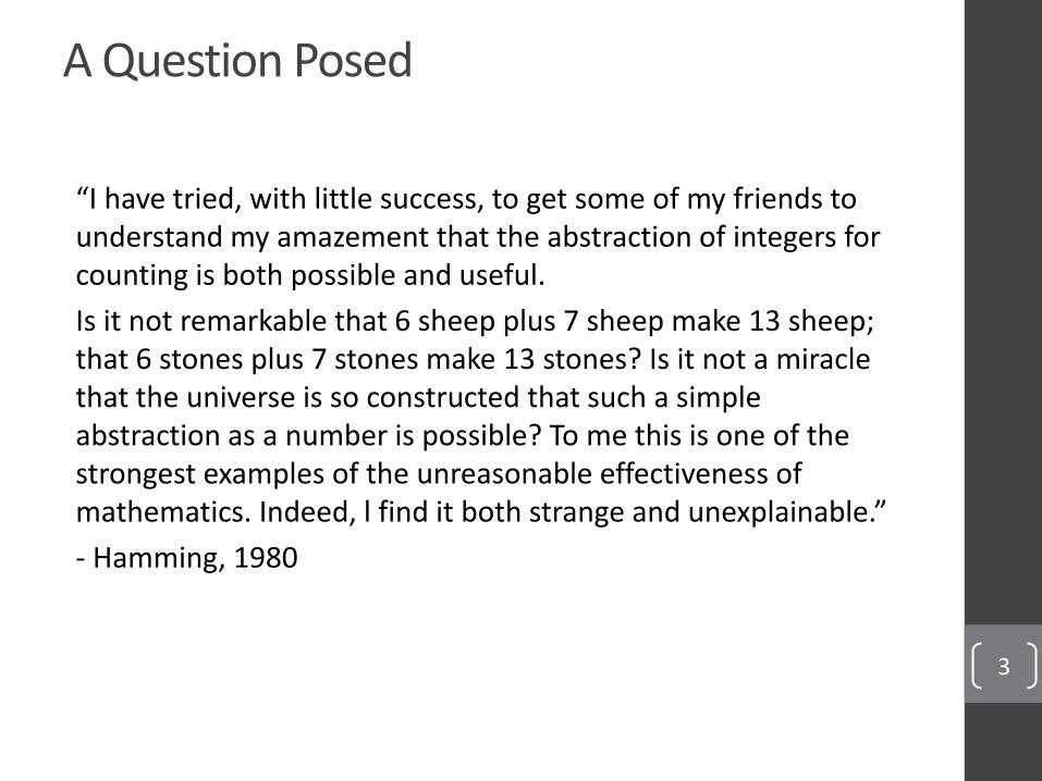
“I have tried, with little success, to get some of my friends to understand my amazement that the abstraction of integers for counting is both possible and useful.
Is it not remarkable that 6 sheep plus 7 sheep make 13 sheep; that 6 stones plus 7 stones make 13 stones? Is it not a miracle that the universe is so constructed that such a simple abstraction as a number is possible? To me this is one of the strongest examples of the unreasonable effectiveness of mathematics. Indeed, l find it both strange and unexplainable.”
- Hamming, 1980
3

A Question Posed
4
2 Pens 4 Pens

A Question Posed
5
2 Pens 4 Pens
2 Pens with 4 Pens

A Question Posed
6
2 Pens 4 Pens
2 Pens with 4 Pens2 ⊕ 4 Pens
How does one determine theoperator ⊕ ?
7
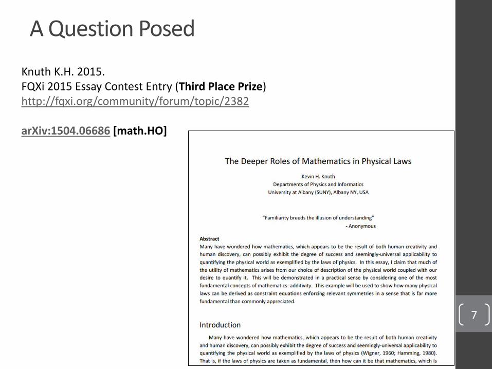
Knuth K.H. 2015. FQXi 2015 Essay Contest Entry (Third Place Prize)http://fqxi.org/community/forum/topic/2382
arXiv:1504.06686 [math.HO]
A Question Posed

8
“Measure that which is measurable and make measureable that which is not” --- Galileo
Our job is to make models of the world around us.
These models are often quantified by consistently assigning numbers so that the quantification captures relevant relationships and symmetries.

9
“Quantum mechanics will cease to look puzzling only when we will be able to derive the formalism of the theory from a set of simple assertions about the world." - Carlo Rovelli
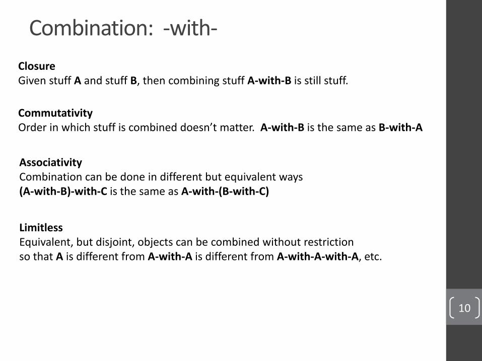
Combination: -with-
10
LimitlessEquivalent, but disjoint, objects can be combined without restrictionso that A is different from A-with-A is different from A-with-A-with-A, etc.
ClosureGiven stuff A and stuff B, then combining stuff A-with-B is still stuff.
CommutativityOrder in which stuff is combined doesn’t matter. A-with-B is the same as B-with-A
AssociativityCombination can be done in different but equivalent ways(A-with-B)-with-C is the same as A-with-(B-with-C)

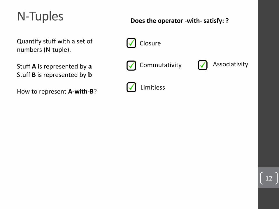
N-Tuples
11
Quantify stuff with a set ofnumbers (N-tuple).
Stuff A is represented by 𝐚Stuff B is represented by 𝐛
How to represent A-with-B?
N-Tuples
12
Closure
Commutativity
Limitless
Associativity
Does the operator -with- satisfy: ?
Quantify stuff with a set ofnumbers (N-tuple).
Stuff A is represented by 𝐚Stuff B is represented by 𝐛
How to represent A-with-B?
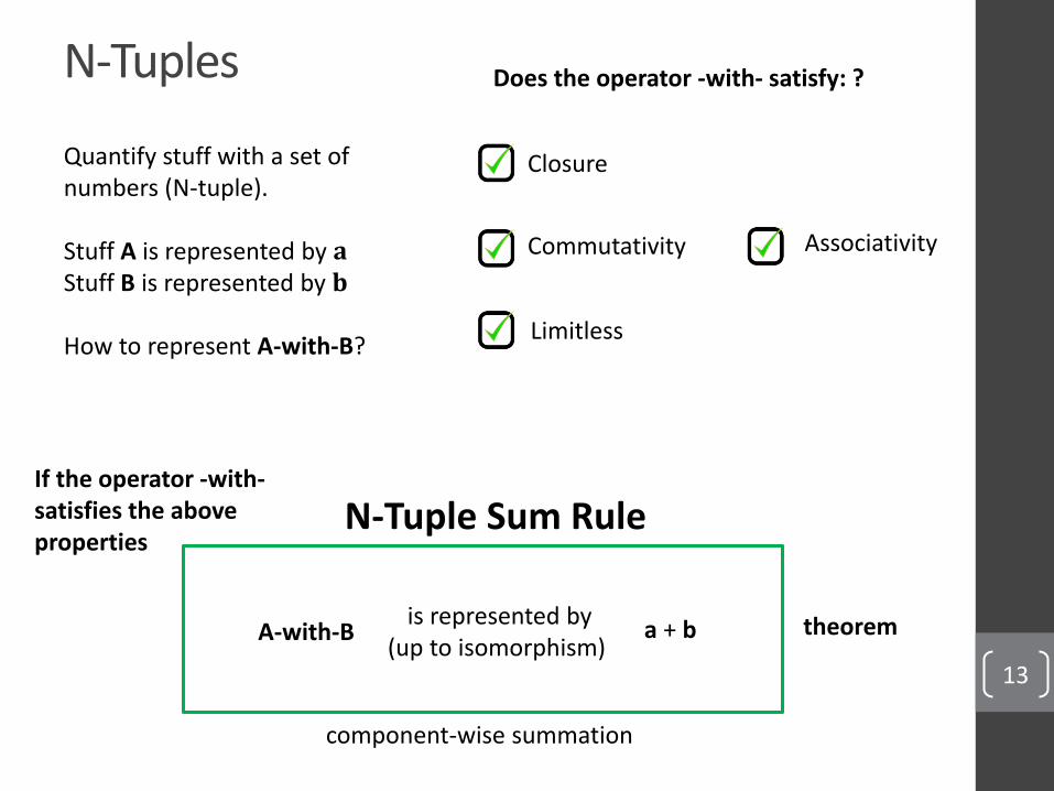
N-Tuples
13
N-Tuple Sum Rule
A-with-Bis represented by
(up to isomorphism) a + b
component-wise summation
Closure
Commutativity
Limitless
Associativity
If the operator -with-satisfies the above properties
Quantify stuff with a set ofnumbers (N-tuple).
Stuff A is represented by 𝐚Stuff B is represented by 𝐛
How to represent A-with-B?
theorem
Does the operator -with- satisfy: ?
Measures
14
CommensurabilityIf stuff has only one relevant property, then quantification requires only onedimension and our vector representation reduces to a scalar.
Measures
15
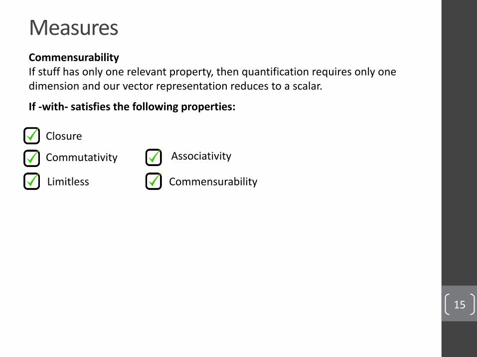
CommensurabilityIf stuff has only one relevant property, then quantification requires only onedimension and our vector representation reduces to a scalar.
If -with- satisfies the following properties:
Closure
Commutativity
Limitless
Associativity
Commensurability
Measures
16
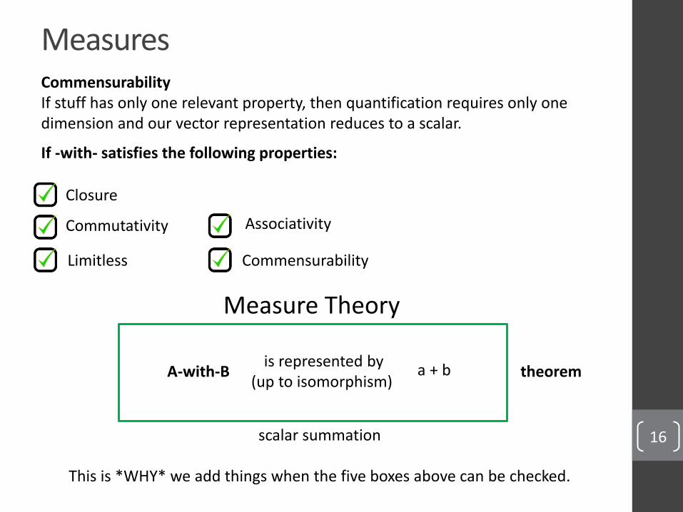
A-with-Bis represented by
(up to isomorphism) a + b
scalar summation
This is *WHY* we add things when the five boxes above can be checked.
CommensurabilityIf stuff has only one relevant property, then quantification requires only onedimension and our vector representation reduces to a scalar.
If -with- satisfies the following properties:
Measure Theory
Closure
Commutativity
Limitless
Associativity
Commensurability
theorem
Combination and Partition
17
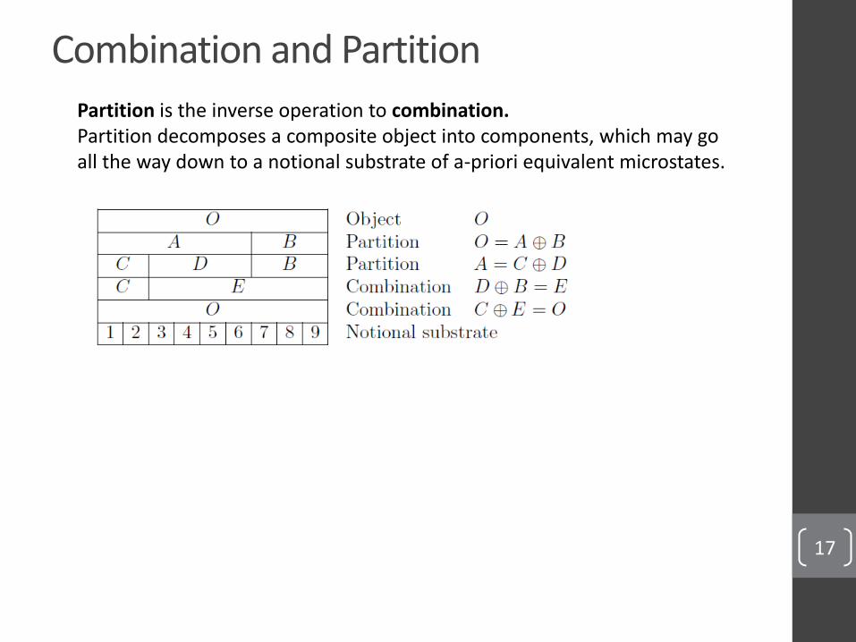
Partition is the inverse operation to combination.Partition decomposes a composite object into components, which may goall the way down to a notional substrate of a-priori equivalent microstates.
Combination and Partition
18
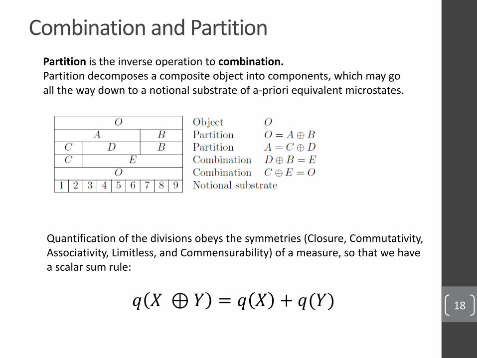
Partition is the inverse operation to combination.Partition decomposes a composite object into components, which may goall the way down to a notional substrate of a-priori equivalent microstates.
Quantification of the divisions obeys the symmetries (Closure, Commutativity,Associativity, Limitless, and Commensurability) of a measure, so that we havea scalar sum rule:
𝑞 𝑋 ⊕ 𝑌 = 𝑞 𝑋 + 𝑞(𝑌)

Steps
19
We are interested in source-to-destination steps: 𝒖 = 𝑑𝑒𝑠𝑡 ; 𝑠𝑜𝑢𝑟𝑐𝑒
ClosureSteps, 𝒖 and 𝒗 can be chained (combined) into a composite step 𝒖 ∘ 𝒗 with a from operator ∘when 𝒖 starts where 𝒗 ends.
Changing the how the steps are combined does not change the result.
𝒖⊕ 𝒗 ∘ 𝒘 = 𝒖 ∘ 𝒘 ⊕ (𝒗 ∘ 𝒘)Right-Distributivity

Steps
20
We are interested in source-to-destination steps: 𝒖 = 𝑑𝑒𝑠𝑡 ; 𝑠𝑜𝑢𝑟𝑐𝑒
ClosureSteps, 𝒖 and 𝒗 can be chained (combined) into a composite step 𝒖 ∘ 𝒗 with a from operator ∘when 𝒖 starts where 𝒗 ends.
Changing the how the steps are combined does not change the result.
𝒖⊕ 𝒗 ∘ 𝒘 = 𝒖 ∘ 𝒘 ⊕ (𝒗 ∘ 𝒘)Right-Distributivity
Right-Distributivity implies that the quantification of a step is linear in the destination. Thus a step can be quantified by
𝑝 𝑋 ; 𝑍 = 𝑞 𝑋 𝑓(𝑍)
where the only remaining freedom is a scale factor that may depend on the source.
Combining Steps
21
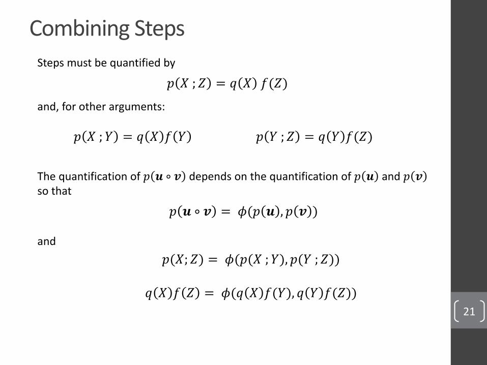
Steps must be quantified by
and, for other arguments:
𝑝 𝑋 ; 𝑌 = 𝑞 𝑋 𝑓 𝑌 𝑝 𝑌 ; 𝑍 = 𝑞 𝑌 𝑓(𝑍)
𝑝 𝑋 ; 𝑍 = 𝑞 𝑋 𝑓(𝑍)
The quantification of 𝑝 𝒖 ∘ 𝒗 depends on the quantification of 𝑝 𝒖 and 𝑝 𝒗so that
𝑝 𝒖 ∘ 𝒗 = 𝜙(𝑝 𝒖 , 𝑝 𝒗 )
and
𝑝(𝑋; 𝑍) = 𝜙(𝑝(𝑋 ; 𝑌), 𝑝(𝑌 ; 𝑍))
𝑞 𝑋 𝑓 𝑍 = 𝜙(𝑞 𝑋 𝑓(𝑌), 𝑞 𝑌 𝑓(𝑍))
Combining Steps
22
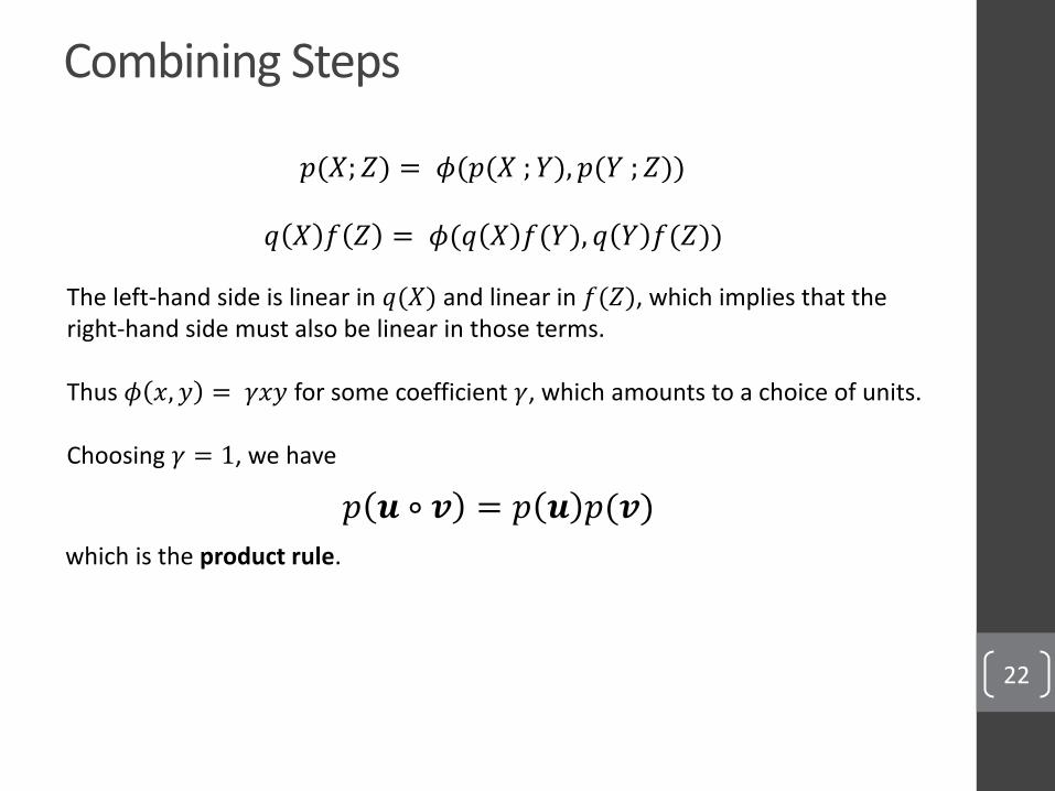
𝑞 𝑋 𝑓 𝑍 = 𝜙(𝑞 𝑋 𝑓(𝑌), 𝑞 𝑌 𝑓(𝑍))
The left-hand side is linear in 𝑞(𝑋) and linear in 𝑓(𝑍), which implies that the right-hand side must also be linear in those terms.
Thus 𝜙 𝑥, 𝑦 = 𝛾𝑥𝑦 for some coefficient 𝛾, which amounts to a choice of units.
Choosing 𝛾 = 1, we have
𝑝 𝒖 ∘ 𝒗 = 𝑝 𝒖 𝑝(𝒗)
𝑝(𝑋; 𝑍) = 𝜙(𝑝(𝑋 ; 𝑌), 𝑝(𝑌 ; 𝑍))
which is the product rule.

Combining Steps
23
𝑞 𝑋 𝑓 𝑍 = 𝜙(𝑞 𝑋 𝑓(𝑌), 𝑞 𝑌 𝑓(𝑍))
Letting 𝑋 = 𝑌 and 𝑍 = 𝑌, we have that
𝑝(𝑋; 𝑍) = 𝜙(𝑝(𝑋 ; 𝑌), 𝑝(𝑌 ; 𝑍))
𝑞(𝑌)𝑓 𝑌 = 𝜙(𝑞 𝑌 𝑓(𝑌), 𝑞 𝑌 𝑓(𝑌))
= 𝛾 [𝑞 𝑌 𝑓(𝑌)]2
So that for 𝛾 = 1 we have that 𝑓 𝑌 = 𝑞−1(𝑌) and
𝑝 𝑑𝑒𝑠𝑡 ; 𝑠𝑜𝑢𝑟𝑐𝑒 =𝑞(𝑑𝑒𝑠𝑡)
𝑞(𝑠𝑜𝑢𝑟𝑐𝑒)
24
“Probability is expectation founded upon partial knowledge”- George Boole
Probability
25
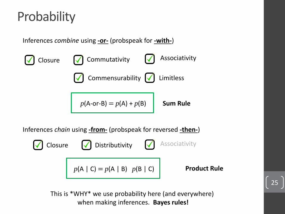
Inferences combine using -or- (probspeak for -with-)
Inferences chain using -from- (probspeak for reversed -then-)
p(A | C) = p(A | B) p(B | C)
p(A-or-B) = p(A) + p(B) Sum Rule
Product Rule
This is *WHY* we use probability here (and everywhere) when making inferences. Bayes rules!
Closure Commutativity
Limitless
Associativity
Commensurability
Closure Distributivity Associativity
26
“This theoretical failure to find a plausible alternative to quantum mechanics, even more than the precise experimental verification of linearity, suggests to me that quantum mechanics is the way it is because any small change in quantum mechanics would lead to logical absurdities.“
- Steven Weinberg

Quantum Theory
27
Our job is to make sense of our observations of objects.
We do not observe objects directly. We observe the interaction between the object and a probe.
As a result, this objective of this theory is to quantify interactions.

Pair Postulate
28
We adopt the pair postulate, where interactions are quantified by two numbers.
Connection with scalar observation is mediated probabilistically through scalar quantities 𝑞(𝜓) arising from the underlying pairs 𝜓.
Detail is lost, which we may try to recover through inference.

Pair Postulate
29
We adopt the pair postulate, where interactions are quantified by two numbers.
Connection with scalar observation is mediated probabilistically through scalar quantities 𝑞(𝜓) arising from the underlying pairs 𝜓.
Detail is lost, which we may try to recover through inference.
Given a production of objects 𝑋, we partition the objects and quantify the extraction of objects 𝑌 by the pair 𝜓 𝑌 𝑋).
𝑋𝑌
𝑍
𝜓(𝑌|𝑋)

Feynman Rules: Sum Rule
30
The Sum Rule for pairs is
𝒖 + 𝒗 =𝑢1 + 𝑣1𝑢2 + 𝑣2
representing
𝜓 𝑋⊕ 𝑌 𝑍) = 𝜓 𝑋 𝑍) + 𝜓 𝑌 𝑍)
𝒖 + 𝒗 𝒖 𝒗

Feynman Rules: Product Rule
31
The Product Rule for pairs is
𝒖 ∘ 𝒗 =
𝑗𝑘
𝛾𝑖𝑗𝑘 𝒖𝑗𝒗𝑘
representing
𝜓 𝑋 𝑍) = 𝜓 𝑋 𝑌) ∘ 𝜓 𝑌 𝑍)
𝒖 ∘ 𝒗 𝒖 𝒗
where 𝛾𝑖𝑗𝑘 represents 8 constant coefficients to be determined.

Feynman Rules: Product Rule
32
The Product Rule for pairs is
𝒖 ∘ 𝒗 =
𝑗𝑘
𝛾𝑖𝑗𝑘 𝒖𝑗𝒗𝑘
where 𝛾𝑖𝑗𝑘 represents 8 constant coefficients to be determined.
Their arbitrariness can be reduced by a linear shear (2 x 2 matrix) instead of the rescaling, or regraduation, that is employed for scalars.
The shear removes four degrees of freedom, leaving four remaining.
Chaining is associative, and associativity reduces the bilinear product rule to Three classes that can be sheared into a standard form (Goyal, Knuth, Skilling 2010)(based on the discriminant 𝜇 = −1, 0, +1)
Feynman Rules: Product Rule
33
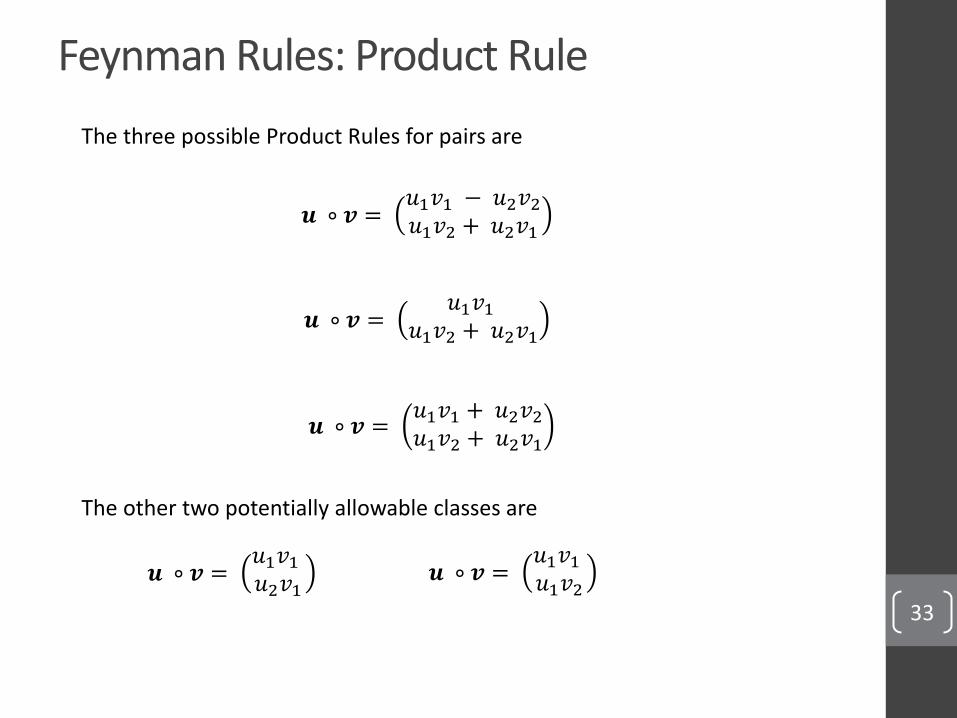
The three possible Product Rules for pairs are
𝒖 ∘ 𝒗 =𝑢1𝑣1 − 𝑢2𝑣2𝑢1𝑣2 + 𝑢2𝑣1
𝒖 ∘ 𝒗 =𝑢1𝑣1
𝑢1𝑣2 + 𝑢2𝑣1
𝒖 ∘ 𝒗 =𝑢1𝑣1 + 𝑢2𝑣2𝑢1𝑣2 + 𝑢2𝑣1
The other two potentially allowable classes are
𝒖 ∘ 𝒗 =𝑢1𝑣1𝑢2𝑣1
𝒖 ∘ 𝒗 =𝑢1𝑣1𝑢1𝑣2
Feynman Rules: Product Rule
34
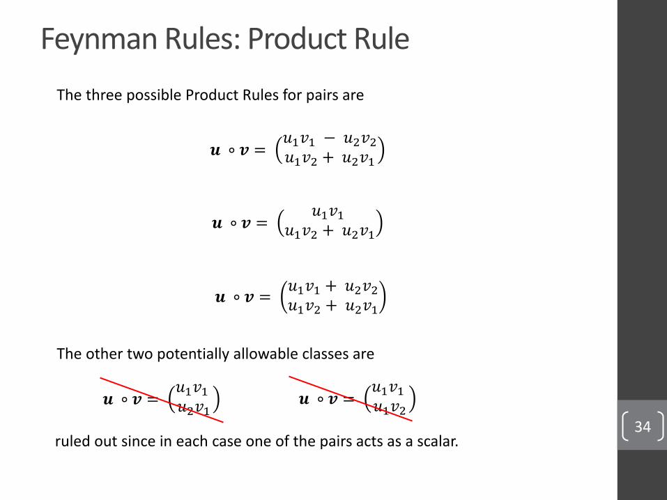
The three possible Product Rules for pairs are
𝒖 ∘ 𝒗 =𝑢1𝑣1 − 𝑢2𝑣2𝑢1𝑣2 + 𝑢2𝑣1
𝒖 ∘ 𝒗 =𝑢1𝑣1
𝑢1𝑣2 + 𝑢2𝑣1
𝒖 ∘ 𝒗 =𝑢1𝑣1 + 𝑢2𝑣2𝑢1𝑣2 + 𝑢2𝑣1
The other two potentially allowable classes are
𝒖 ∘ 𝒗 =𝑢1𝑣1𝑢2𝑣1
𝒖 ∘ 𝒗 =𝑢1𝑣1𝑢1𝑣2
ruled out since in each case one of the pairs acts as a scalar.
Feynman Rules: Product Rule
35
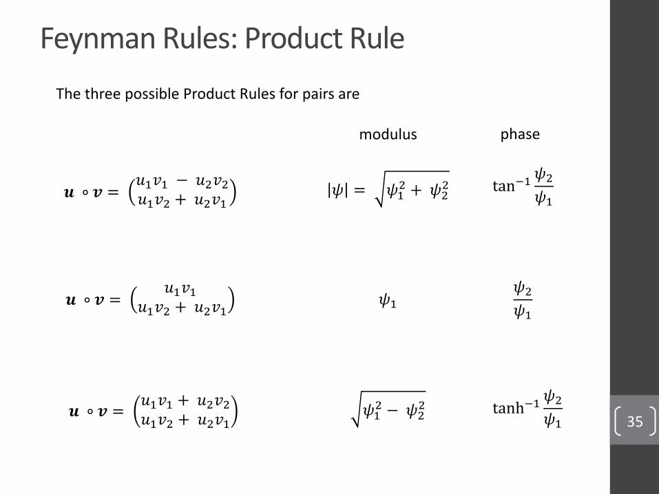
The three possible Product Rules for pairs are
𝒖 ∘ 𝒗 =𝑢1𝑣1 − 𝑢2𝑣2𝑢1𝑣2 + 𝑢2𝑣1
𝒖 ∘ 𝒗 =𝑢1𝑣1
𝑢1𝑣2 + 𝑢2𝑣1
𝒖 ∘ 𝒗 =𝑢1𝑣1 + 𝑢2𝑣2𝑢1𝑣2 + 𝑢2𝑣1
𝜓 = 𝜓12 + 𝜓2
2 tan−1𝜓2
𝜓1
𝜓1
𝜓2
𝜓1
𝜓12 − 𝜓2
2 tanh−1𝜓2
𝜓1
modulus phase
Feynman Rules: Product Rule
36
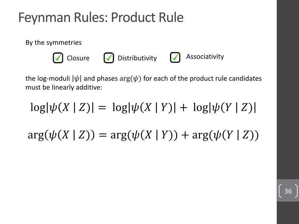
By the symmetries
the log-moduli 𝜓 and phases arg(𝜓) for each of the product rule candidatesmust be linearly additive:
Closure Distributivity Associativity
log 𝜓 𝑋 𝑍) = log 𝜓 𝑋 𝑌) + log 𝜓 𝑌 𝑍)
arg 𝜓 𝑋 𝑍) = arg(𝜓 𝑋 𝑌)) + arg(𝜓 𝑌 𝑍))

Feynman Rules: Product Rule
37
log 𝜓 𝑋 𝑍) = log 𝜓 𝑋 𝑌) + log 𝜓 𝑌 𝑍)
arg 𝜓 𝑋 𝑍) = arg(𝜓 𝑋 𝑌)) + arg(𝜓 𝑌 𝑍))
The only freedom between conforming linear scales is a constant factor,so there exists a common scale (based on the symmetries) on which we may place our scalar
log 𝑞 = 𝛼 log 𝜓 + 𝛽 arg(𝜓)for some constants 𝛼 and 𝛽.
Feynman Rules: Product Rule
38
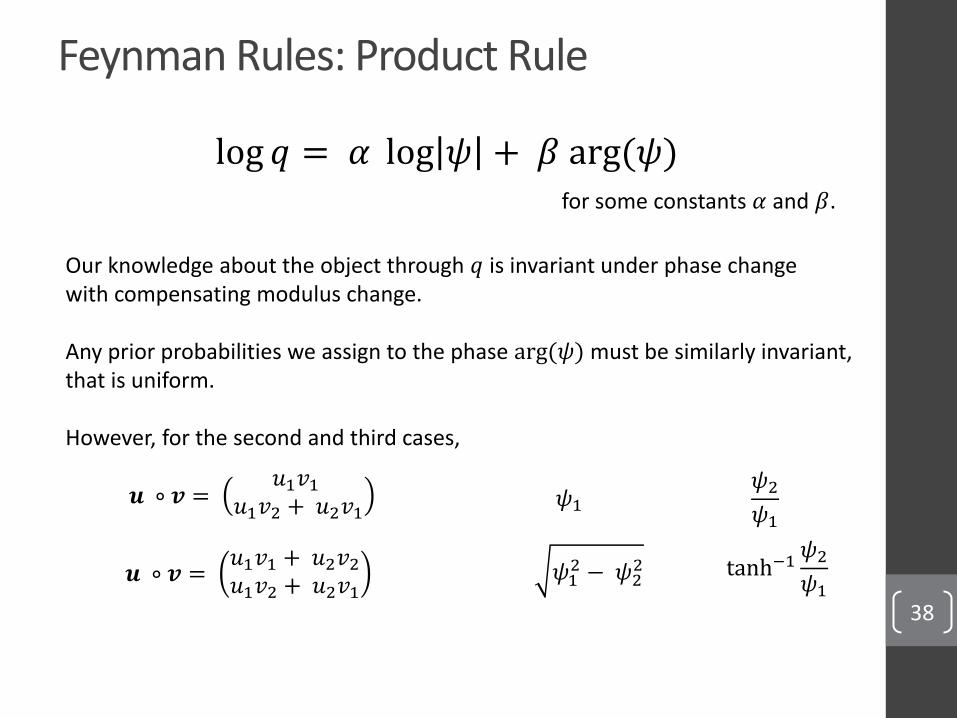
log 𝑞 = 𝛼 log 𝜓 + 𝛽 arg(𝜓)for some constants 𝛼 and 𝛽.
Our knowledge about the object through 𝑞 is invariant under phase change with compensating modulus change.
Any prior probabilities we assign to the phase arg(𝜓) must be similarly invariant,that is uniform.
However, for the second and third cases,
𝒖 ∘ 𝒗 =𝑢1𝑣1
𝑢1𝑣2 + 𝑢2𝑣1𝜓1
𝜓2
𝜓1
𝒖 ∘ 𝒗 =𝑢1𝑣1 + 𝑢2𝑣2𝑢1𝑣2 + 𝑢2𝑣1
𝜓12 − 𝜓2
2 tanh−1𝜓2
𝜓1

Feynman Rules: Product Rule
39
log 𝑞 = 𝛼 log 𝜓 + 𝛽 arg(𝜓)for some constants 𝛼 and 𝛽.
Our knowledge about the object through 𝑞 is invariant under phase change with compensating modulus change.
Any prior probabilities we assign to the phase arg(𝜓) must be similarly invariant,that is uniform.
However, for the second and third cases,
the phase has infinite range making the priors improper and inference impossible.
𝒖 ∘ 𝒗 =𝑢1𝑣1
𝑢1𝑣2 + 𝑢2𝑣1𝜓1
𝜓2
𝜓1
𝒖 ∘ 𝒗 =𝑢1𝑣1 + 𝑢2𝑣2𝑢1𝑣2 + 𝑢2𝑣1
𝜓12 − 𝜓2
2 tanh−1𝜓2
𝜓1

Feynman Rules: Product Rule
40
We are then left with a single possible Product Rule
𝒖 ∘ 𝒗 =𝑢1𝑣1 − 𝑢2𝑣2𝑢1𝑣2 + 𝑢2𝑣1
𝒖 ∘ 𝒗 =𝑢1𝑣1
𝑢1𝑣2 + 𝑢2𝑣1
𝒖 ∘ 𝒗 =𝑢1𝑣1 + 𝑢2𝑣2𝑢1𝑣2 + 𝑢2𝑣1
𝜓 = 𝜓12 + 𝜓2
2 tan−1𝜓2
𝜓1
𝜓1
𝜓2
𝜓1
𝜓12 − 𝜓2
2 tanh−1𝜓2
𝜓1
modulus phase
infinite rangeimproper prior
infinite rangeimproper prior
Ranges from 0 to 2𝜋proper prior!
Quantum Mechanics: Scalar Measure
41
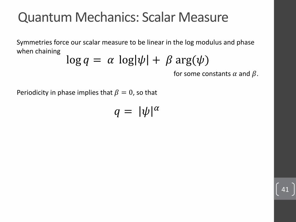
log 𝑞 = 𝛼 log 𝜓 + 𝛽 arg(𝜓)for some constants 𝛼 and 𝛽.
Symmetries force our scalar measure to be linear in the log modulus and phase when chaining
Periodicity in phase implies that 𝛽 = 0, so that
𝑞 = 𝜓 𝛼
Quantum Mechanics: Scalar Measure
42
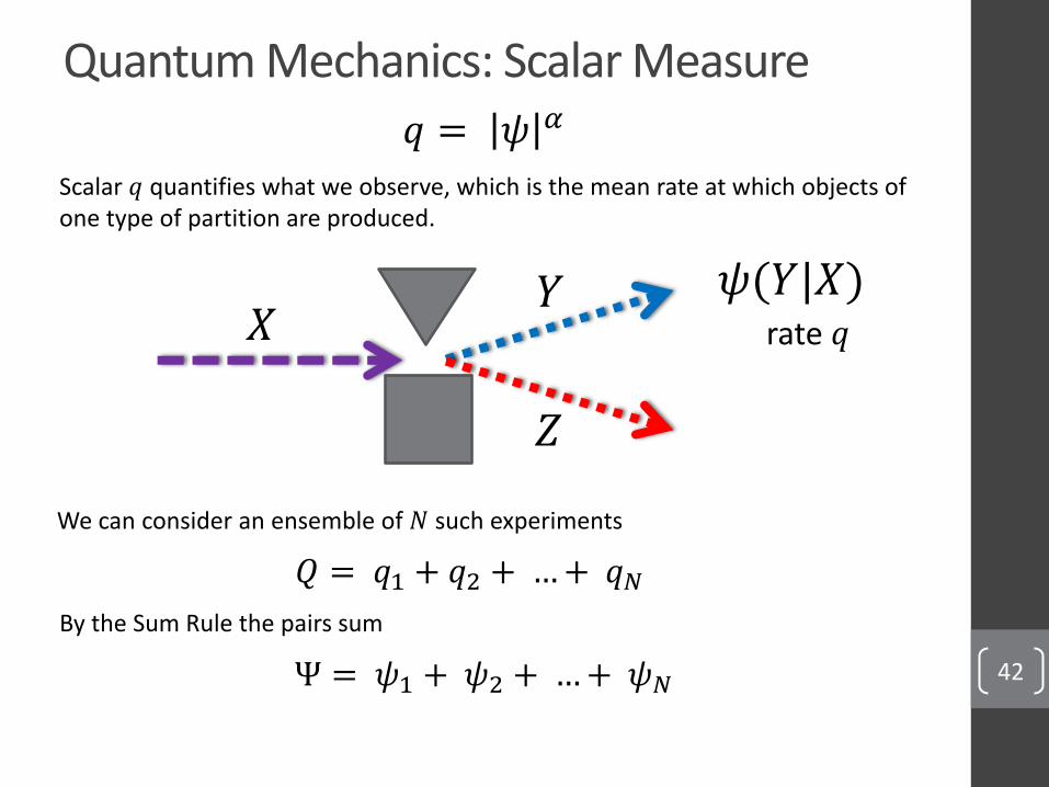
𝑞 = 𝜓 𝛼
𝑋𝑌
𝑍
𝜓(𝑌|𝑋)
Scalar 𝑞 quantifies what we observe, which is the mean rate at which objects ofone type of partition are produced.
rate 𝑞
𝑄 = 𝑞1 + 𝑞2 + …+ 𝑞𝑁
We can consider an ensemble of 𝑁 such experiments
By the Sum Rule the pairs sum
Ψ = 𝜓1 + 𝜓2 + …+ 𝜓𝑁
Quantum Mechanics: Born Rule
43
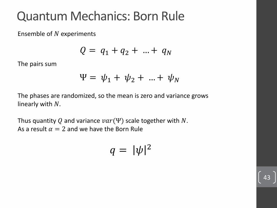
𝑞 = 𝜓 2
𝑄 = 𝑞1 + 𝑞2 + …+ 𝑞𝑁
Ensemble of 𝑁 experiments
The pairs sum
Ψ = 𝜓1 + 𝜓2 + …+ 𝜓𝑁
The phases are randomized, so the mean is zero and variance grows linearly with 𝑁.
Thus quantity 𝑄 and variance 𝑣𝑎𝑟(Ψ) scale together with 𝑁.As a result 𝛼 = 2 and we have the Born Rule
Probability Assignments
44
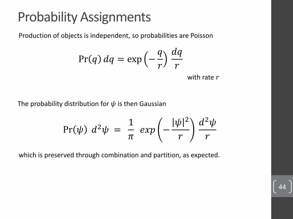
Production of objects is independent, so probabilities are Poisson
Pr 𝑞 𝑑𝑞 = exp −𝑞
𝑟
𝑑𝑞
𝑟with rate 𝑟
The probability distribution for 𝜓 is then Gaussian
Pr 𝜓 𝑑2𝜓 =1
𝜋𝑒𝑥𝑝 −
𝜓 2
𝑟
𝑑2𝜓
𝑟
which is preserved through combination and partition, as expected.
Measure, Probability, Quantum
45
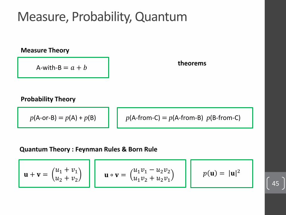
𝑝 𝐮 = 𝐮 2𝐮 ∘ 𝐯 =
𝑢1𝑣1 − 𝑢2𝑣2𝑢1𝑣2 + 𝑢2𝑣1
𝐮 + 𝐯 =𝑢1 + 𝑣1𝑢2 + 𝑣2
Measure Theory
Probability Theory
Quantum Theory : Feynman Rules & Born Rule
A-with-B = 𝑎 + 𝑏
p(A-or-B) = p(A) + p(B) p(A-from-C) = p(A-from-B) p(B-from-C)
theorems
“Quantum Mechanics will cease to look puzzling only when we will be able to derive the formalism of the theory from a set of simple physical assertions about the world.”
- Carlo Rovelli
46
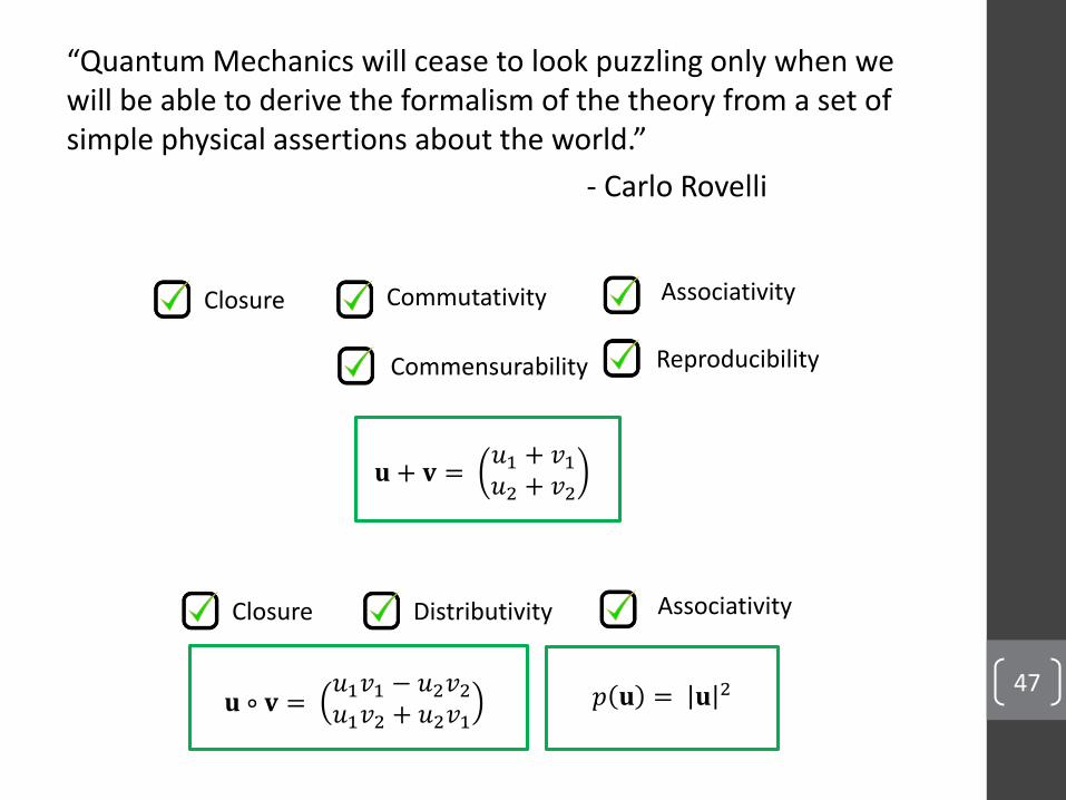
“Quantum Mechanics will cease to look puzzling only when we will be able to derive the formalism of the theory from a set of simple physical assertions about the world.”
- Carlo Rovelli
47
Closure Commutativity
Reproducibility
Associativity
Commensurability
𝐮 + 𝐯 =𝑢1 + 𝑣1𝑢2 + 𝑣2
Closure Distributivity Associativity
𝑝 𝐮 = 𝐮 2𝐮 ∘ 𝐯 =
𝑢1𝑣1 − 𝑢2𝑣2𝑢1𝑣2 + 𝑢2𝑣1

Quantum Mechanics
48
We use combination and partition to construct a corresponding pattern of partially-known complex amplitudes and associated probabilities, as dictated by simple symmetries.
We then use standard probabilistic inference to restrict those possibilities in accordance with observations, thereby gaining predictive power over what our detectors will record.
That is what Quantum Mechanics is.
𝑝 𝐮 = 𝐮 2
𝐮 = 𝐯1 + 𝐯2 + 𝐯3 + 𝐯4
𝐮
𝐯1𝐯2𝐯3𝐯4

49
THANK YOU
Ariel Caticha, Seth Chaiken, Keith Earle, Anton Garrett, Steve Gull, Oleg Lunin, Andrei Khrennikov, Julio Stern, Federico Holik, FQXi, and Ed Jaynes!