2 Mean-Field Theory: Hartree-Fock and BCS

Erik KochInstitute for Advanced SimulationForschungszentrum Julich

Contents

1 Many-electron states 2

2 Second quantization 52.1 Creation and annihilation operators . . . . . . . . . . . . . . . . . . . . . . . . 52.2 Representation of Slater determinants . . . . . . . . . . . . . . . . . . . . . . 72.3 Representation of n-body operators . . . . . . . . . . . . . . . . . . . . . . . 92.4 Reduced density matrices and Wick’s theorem . . . . . . . . . . . . . . . . . . 11

3 Variational methods 143.1 Non-interacting electrons . . . . . . . . . . . . . . . . . . . . . . . . . . . . . 153.2 Hartree-Fock theory . . . . . . . . . . . . . . . . . . . . . . . . . . . . . . . . 163.3 BCS theory . . . . . . . . . . . . . . . . . . . . . . . . . . . . . . . . . . . . 26

4 Conclusion 29

A Basis orthonormalization 30

B Some useful commutation relations 31

C Pauli matrices and spin rotations 32

E. Pavarini, E. Koch, J. van den Brink, and G. Sawatzky (eds.)Quantum Materials: Experiments and TheoryModeling and Simulation Vol. 6Forschungszentrum Julich, 2016, ISBN 978-3-95806-159-0http://www.cond-mat.de/events/correl16

2.2 Erik Koch

1 Many-electron states

One of the deepest mysteries of physics is that all the different objects that surround us are builtfrom a small set of indistinguishable particles. The very existence of such elementary particlesthat have all their properties in common is a direct consequence of quantum physics. Classicalobjects can always be distinguished by their location in space. This lead Leibniz to formulatehis Principle of the Identity of Indiscernibles [1]. For quantum objects, however, the uncertaintyprinciple makes the distinction of particles by their position impossible. Indistinguishability ofquantum objects then means that there is no measurement that would let us tell them apart,i.e., all expectation values 〈Ψ |M |Ψ〉 must remain the same when we change the labeling of thedistinct but indistinguishable the particles.

The consequences for observables are straightforward: An observable M(x) acting on a single-particle degree of freedom x must operate on all indistinguishable particles in the same way,i.e.,

∑iM(xi). A two-body observable M(x, x′) must operate on all pairs in the same way,∑

i,jM(xi, xj) with M(x, x′) = M(x′, x). We can thus write any observable in the form

M(x) = M (0) +∑i

M (1)(xi) +1

2!

∑i6=j

M (2)(xi, xj) +1

3!

∑i6=j 6=k

M (3)(xi, xj, xk) + · · · (1)

= M (0) +∑i

M (1)(xi) +∑i<j

M (2)(xi, xj) +∑i<j<k

M (3)(xi, xj, xk) + · · · , (2)

where the summations can be restricted since the operators must be symmetric in their argu-ments, e.g. M (2)(xi, xj) = M (2)(xj, xi), while for two or more identical coordinates the opera-tor is really one of lower order: M (2)(xi, xi), e.g., only acts on a single coordinate and shouldbe included in M (1).

For the many-body wave functions Ψ(x1, x2, · · · ) the situation is slightly more complex. Sincethe probability density |Ψ(x1, x2, · · · )|2 is an observable, they should transform as one-dimen-sional (irreducible) representations, i.e., either be symmetric or antisymmetric under particlepermutations. Which of the two options applies to a given elementary particle is determinedby the spin-statistics theorem [2, 3]: The wave functions of particles with integer spin are sym-metric, those of particles with half-integer spin change sign wen arguments are exchanged.From an arbitrary N -particle wave function we thus obtain a many-electron wavefunction byantisymmetrizing

S− Ψ(x1, . . . , xN) :=1√N !

∑P

(−1)PΨ(xp(1), . . . , xp(N)

), (3)

where (−1)P is the parity of the permutation P that maps n→ p(n). Since there areN ! differentpermutations, this can easily become an extremely costly operation. Remarkably, a product ofN single-electron states ϕα can be antisymmetrized much more efficiently (in O(N3) steps) by

Hartree-Fock and BCS 2.3

writing it in the form of a determinant

Φα1,...,αN (x1, . . . , xN) :=1√N !

∣∣∣∣∣∣∣∣∣∣ϕα1(x1) ϕα2(x1) · · · ϕαN (x1)

ϕα1(x2) ϕα2(x2) · · · ϕαN (x2)...

... . . . ...ϕα1(xN) ϕα2(xN) · · · ϕαN (xN)

∣∣∣∣∣∣∣∣∣∣. (4)

For N = 1 the Slater determinant is simply the one-electron orbital Φα(x) = ϕα(x) and forN = 2 we get the familiar two-electron Slater determinant Φα,α′(x, x′) = (ϕα(x)ϕα′(x

′) −ϕα′(x)ϕα(x′))/

√2.

Slater determinants are important because they can be used to build a basis of the many-electronHilbert space. To see how, we consider a complete set of orthonormal single-electron states∫

dxϕn(x)ϕm(x) = δn,m (orthonormal)∑n

ϕn(x)ϕn(x′) = δ(x− x′) (complete) . (5)

To expand an arbitrary N -particle function a(x1, . . . , xN), we start by considering it as a func-tion of x1 with x2, . . . , xN kept fixed. We can then expand it in the complete set {ϕn} as

a(x1, . . . , xN) =∑n1

an1(x2, . . . , xN)ϕn1(x1)

with expansion coefficients

an1(x2, . . . , xN) =

∫dx ϕn1(x1) a(x1, x2, . . . , xN) .

These, in turn, can be expanded as a functions of x2

an1(x2, . . . , xN) =∑n2

an1,n2(x3, . . . , xN)ϕn2(x2) .

Repeating this, we obtain the expansion of a in product states

a(x1, . . . , xN) =∑

n1,...,nN

an1,...,nN ϕn1(x1) · · ·ϕnN (xN) .

When the N -particle function Ψ is antisymmetric, the expansion coefficients will be antisym-metric under permutation of the indices anp(1),...,np(N)

= (−1)Pan1,...,nN . Fixing an order of theindices, e.g., n1 < n2 < . . . < nN , we thus get an expansion in Slater determinants

Ψ(x1, . . . , xN) =∑

n1<...<nN

√N ! an1,...,nN Φn1,...,nN (x1, . . . , xN) .

Since we can write any antisymmetric function as such a configuration-interaction expansion,the set of Slater determinants{

Φn1,...,nN (x1, . . . , xN)∣∣∣ n1 < n2 < · · · < nN

}(6)

2.4 Erik Koch

forms a basis of the N -electron Hilbert space. Since the overlap of two Slater determinants∫dx Φα1,...,αN (x)Φβ1,...,βN (x) =

1

N !

∑P,P ′

(−1)P+P ′∏n

∫dxn ϕαp(n)(xn)ϕαp′(n)(xn)

= 〈Φα1,...,αN |Φβ1,...,βN 〉 =

∣∣∣∣∣∣∣〈ϕα1|ϕβ1〉 · · · 〈ϕα1|ϕβN 〉

... . . . ...〈ϕαN |ϕβ1〉 · · · 〈ϕαN |ϕβN 〉

∣∣∣∣∣∣∣ (7)

is the determinant of the overlap of the constituent orbitals, the Slater determinants (6) forma complete orthonormal basis of the N -electron Hilbert space when the orbitals ϕn(x) are acomplete orthonormal basis of the one-electron Hilbert space.While we use a set of N one-electron orbitals ϕn(x) to define an N -electron Slater determinantΦα1,...,αN (x) (4), this representation is not unique: Any unitary transformation among the Noccupied orbitals will not change the determinant. Thus, strictly, a Slater determinant is notdetermined by the set of indices we usually give, but, up to a phase, by the N -dimensionalsubspace spanned by the orbitals ϕ1, . . . , ϕN in the single-electron Hilbert space. The projectorto this space is the one-body density matrix

Γ (1)(x, x′) = N

∫dx2 · · · dxN Φ(x, x2, . . . , xN)Φ(x′, x2, . . . , xN) . (8)

To see this, we expand the Slater determinant along its first row

Φα1···αN (x1, . . . , xN) =1√N

N∑n=1

(−1)1+n ϕαn(x1)Φαi6=n(x2, . . . , xN) , (9)

where Φαi6=n(x2, . . . , xN) is the determinant with the first row and the n-th column removed,which can be written as N−1-electron Slater determinants with orbital αn removed. Insertingthis into (8) we find

Γ(1)Φ (x, x′) =

N∑n=1

ϕαn(x)ϕαn(x′) , (10)

which is the expansion of the one-body density matrix in eigenfunctions (natural orbitals) show-ing that its eigenvalues (natural occupation numbers) are one. Any many-electron wave functionΨ(x) with the same one-body density matrix Γ (1)

Φ equals Φ(x) up to a phase, i.e., |〈Ψ |Φ〉| = 1.We can generalize this procedure and calculate higher order density matrices by introducing thegeneralized Laplace expansion

Φα1···αN (x) =1√(Np

) ∑n1<···<np

(−1)1+∑i ni Φαn1 ···αnp (x1, . . . , xp)Φαi6∈{n1,...,np}(xp+1, . . . , xN),

which is obtained by writing the permutation of all N indices as a permutation of N −p indicesand the remaining p indices separately summing over all distinct sets of p indices. This allowsus to evaluate arbitrary matrix elements and higher order density matrices [4]. But as can beseen from the above expansion, the expressions very quickly get quite cumbersome. Fortunatelythere is a representation that is much better suited to handling antisymmetric wave functions. Itis called second quantization.

Hartree-Fock and BCS 2.5

2 Second quantization

While originally introduced for quantizing the electromagnetic field, we can use the formalismof second quantization just as a convenient way of handling antisymmetric wave functions [5,6].The idea behind this approach is remarkably simple: When writing Slater determinants in theform (4) we are working in a real-space basis. It is, however, often better not to work in aspecific basis but to consider abstract states: Instead of a wave function ϕα(x), we write a Diracstate |α〉. Second quantization allows us to do the same for Slater determinants.Let us consider a Slater determinant for two electrons, one in state ϕα(x), the other in stateϕβ(x). It is simply the antisymmetrized product of the two states

Φαβ(x1, x2) =1√2

(ϕα(x1)ϕβ(x2)− ϕβ(x1)ϕα(x2)

). (11)

This expression is quite cumbersome because we explicitly specify the coordinates. We can getrid of the coordinates by defining a two-particle Dirac state

|α, β〉 :=1√2

(|α〉|β〉 − |β〉|α〉

).

While the expression is already simpler, we still have to keep track of the order of the particlesby specifying the position of the kets. The idea of second quantization is to specify the statesusing operators

c†βc†α|0〉 = |α, β〉 . (12)

Now the order of the particles is specified by the order of the operators. To ensure the antisym-metry of the wave function the operators have to change sign when they are reordered

|α, β〉 = c†βc†α|0〉 = −c†αc

†β|0〉 = −|β, α〉 . (13)

Naturally, this also implies the Pauli principle for the special case β = α.

2.1 Creation and annihilation operators

To arrive at the formalism of second quantization we postulate a set of operators that havecertain reasonable properties. We then verify that we can use these operators to represent Slaterdeterminants. But first we consider a few simple states to motivate what properties the newoperators should have.To be able to construct many-electron states we start from the simplest such state: |0〉 thevacuum state with no electron, which we assume to be normalized 〈0|0〉 = 1. Next we introducefor each single-electron state |α〉 an operator c†α such that c†α|0〉 = |α〉. These operators arecalled creation operators since they add an electron (in state α) to the state that they act on:in c†α|0〉 the creation operator adds an electron to the vacuum state (N = 0), resulting in asingle-electron state. Applying another creation operator produces a two-electron state c†βc

†α|0〉.

As we have seen above, to ensure the antisymmetry of the two electron state, the product of

2.6 Erik Koch

creation operators has to change sign when they are reordered: c†αc†β = −c†βc†α. This is more

conveniently written as {c†α, c†β} = 0 by introducing the anti-commutator

{A, B} := AB +BA . (14)

As we have seen, the simplest state we can produce with the creation operators is the single-electron state |α〉 = c†α|0〉. When we want to calculate its norm, we have to consider theadjoint of c†α|0〉, formally obtaining 〈α|α〉 = 〈0|cαc†α|0〉, or, more generally, 〈α|β〉 = 〈0|cαc

†β|0〉.

This must mean that cα, the adjoint of a creation operator, must remove an electron from thestate, otherwise the overlap of cαc

†β|0〉 with the vacuum state 〈0| would vanish. We therefore

call the adjoint of the creation operator an annihilation operator. We certainly cannot take anelectron out of the vacuum state, so cα|0〉 = 0. To obtain the correct overlap of one-electronstates as 〈α|β〉 = 〈0|cαc

†β|0〉 we postulate the anticommutation relation {cα, c

†β} = 〈α|β〉. For

completeness, taking the adjoint of the anticommutation relation for the creation operators, weobtain the corresponding anticommutator of the annihilators: {cα, cβ} = 0.Thus, we define the vacuum state |0〉 and the set of operators cα related to single-electron states|α〉 with the properties

cα|0〉 = 0{cα, cβ

}= 0 =

{c†α, c

†β

}〈0|0〉 = 1

{cα, c

†β

}= 〈α|β〉

(15)

We note that the creators and annihilators are not ordinary operators in a Hilbert space, buttransfer states from an N -electron to a N ± 1-electron Hilbert space, i.e., they are operatorsdefined on Fock space. It is also remarkable that the mixed anti-commutator is the only placewhere the orbitals that distinguish different operators enter. Moreover, despite being operators,the creators transform in the same way as the single-electron states they represent while thevacuum state is invariant:

|αi〉 =∑µ

|αµ〉Uµi ; c†αi|0〉 =∑µ

c†αµ |0〉Uµi =

(∑µ

c†αµUµi

)|0〉. (16)

A set of operators that allows us to make contact with the notation of first quantization are thefield operators Ψ †(x), with x = (r, σ), that create an electron of spin σ at position r, i.e., instate |x〉 = |r, σ〉. Given a complete, orthonormal set of orbitals {ϕn}, we can expand |x〉

Ψ †(x)|0〉 = |x〉 =∑n

|ϕn〉〈ϕn|x〉 =∑n

〈ϕn|x〉 c†ϕn|0〉 (17)

from which we obtain

Ψ †(x) =∑n

〈x|ϕn〉 c†ϕn =∑n

ϕn(x) c†ϕn . (18)

The anticommutators then follow from (15) for an orthonormal and complete set, e.g.,{Ψ(x), Ψ †(x′)

}=∑n,m

〈x|ϕn〉{cϕn , c

†ϕm

}︸ ︷︷ ︸=δn,m

〈ϕm|x′〉 =∑n

〈x|ϕn〉〈ϕn|x′〉 = 〈x|x′〉 = δ(x− x′),

Hartree-Fock and BCS 2.7

resulting in the anticommutation relations for the field operators{Ψ(x), Ψ(x′)

}= 0 =

{Ψ †(x), Ψ †(x′)

}and

{Ψ(x), Ψ †(x′)

}= 〈x|x′〉. (19)

We can, of course, expand the field operators also in a non-orthogonal set of orbitals {|χi〉}, aslong as it is complete,

∑i,j |χi〉(S−1)ij〈χj| = 1, where Sij = 〈χi|χj〉 is the overlap matrix

Ψ †(x) =∑i,j

c†i (S−1)ij 〈χj|x〉. (20)

Conversely, given any single-electron wave functions in real space ϕ(x), we can express thecorresponding creation operator in terms of the field operators

c†ϕ =

∫dxϕ(x) Ψ †(x). (21)

Its anticommutator with the field operators just gives back the single-electron wave function

{Ψ(x), c†ϕ

}=

∫dx′ ϕ(x′)

{Ψ(x), Ψ †(x′)

}= ϕ(x) . (22)

2.2 Representation of Slater determinants

We have now all the tools in place to write the Slater determinant (4) in second quantization,using the creation operators to specify the occupied orbitals and the field operators to define thecoordinates for the real-space representation

Φα1α2...αN (x1, x2, . . . , xN) =1√N !

⟨0∣∣∣ Ψ(x1)Ψ(x2) . . . Ψ(xN) c†αN . . . c

†α2c†α1

∣∣∣ 0⟩ . (23)

Not surprisingly, the proof is by induction. As a warm-up we consider the case of a single-electron wave function (N = 1). Using the anticommutation relation (22), we see that⟨

0∣∣∣ Ψ(x1) c†α1

∣∣∣ 0⟩ =⟨

0∣∣∣ϕα1(x1)− c†α1

Ψ(x1)∣∣∣ 0⟩ = ϕα1(x1) . (24)

For the two-electron state N = 2, we anticommute Ψ(x2) in two steps to the right⟨0∣∣∣ Ψ(x1)Ψ(x2) c†α2

c†α1

∣∣∣ 0⟩ =⟨

0∣∣∣ Ψ(x1)

(ϕα2(x2)− c†α2

Ψ(x2))c†α1

∣∣∣ 0⟩=

⟨0∣∣∣ Ψ(x1)c†α1

∣∣∣ 0⟩ ϕα2(x2)−⟨

0∣∣∣ Ψ(x1)c†α2

Ψ(x2)c†α1

∣∣∣ 0⟩= ϕα1(x1)ϕα2(x2)− ϕα2(x1)ϕα1(x2) . (25)

We see how anticommuting automatically produces the appropriate signs for the antisymmetricwave function. Dividing by

√2, we obtain the desired two-electron Slater determinant.

2.8 Erik Koch

The general case of an N -electron state works just the same. Anti-commuting Ψ(xN) all theway to the right produces N − 1 terms with alternating sign⟨

0∣∣∣ Ψ(x1) . . . Ψ(xN−1)Ψ(xN) c†αN c

†αN−1

. . . c†α1

∣∣∣ 0⟩ =

+⟨

0∣∣∣ Ψ(x1) . . . Ψ(xN−1) c†αN−1

. . . c†α1

∣∣∣ 0⟩ ϕαN (xN)

−⟨

0∣∣∣ Ψ(x1) . . . Ψ(xN−1)

∏n6=N−1 c

†αn

∣∣∣ 0⟩ ϕαN−1(xN)

...

(−1)N⟨

0∣∣∣ Ψ(x1) . . . Ψ(xN−1) c†αN . . . c†α2

∣∣∣ 0⟩ ϕα1 (xN) .

Using (23) for the N − 1-electron states, this is nothing but the Laplace expansion of

D =

∣∣∣∣∣∣∣∣∣∣ϕα1(x1) ϕα2(x1) · · · ϕαN (x1)

ϕα1(x2) ϕα2(x2) · · · ϕαN (x2)...

... . . . ...ϕα1(xN) ϕα2(xN) · · · ϕαN (xN)

∣∣∣∣∣∣∣∣∣∣along the N th row. Dividing by

√N ! we see that we have shown (23) for N -electron states,

completing the proof by induction.Thus, as we can write the representation of a single-electron state |ϕ〉 in real-space as the matrixelement 〈x|ϕ〉 = ϕ(x), we can obtain the representation of the N -electron

∏c†αn |0〉 as the

matrix element with the field operators 〈0|∏Ψ(xn). Thus, we can rewrite the basis (6) for the

N -electron states in a form independent of the real-space representation{c†nN · · · c

†n1|0〉∣∣ n1 < · · · < nN

}, (26)

which allows us to write any N -electron state as

|Ψ〉 =∑

n1<···<nN

an1,...,nN c†nN· · · c†n1

|0〉. (27)

From this we see that, for an orthonormal basis, the expectation value of the occupation numberoperator ni = c†ici is the probability that state ϕni is occupied

〈Ψ |ni|Ψ〉 =∑

ni∈{n1<···<nN}

|an1,...,nN |2, (28)

since only determinants that contain ϕni contribute. The sum of all these operators N =∑

i niis the number operator, since now each determinant contributes N times

〈Ψ |∑i

ni|Ψ〉 =∑i

∑ni∈{n1<···<nN}

|an1,...,nN |2 = N . (29)

For the special case of the field operators we obtain the density operator n(x) = Ψ †(x)Ψ(x) andN =

∫dx Ψ †(x)Ψ(x).

Hartree-Fock and BCS 2.9

2.3 Representation of n-body operators

Having established the relation between product states and Slater determinants, it is straightfor-ward to express the matrix elements of a general n-body operator (2)

M(x) = M (0) +∑i

M (1)(xi) +∑i<j

M (2)(xi, xj) +∑i<j<k

M (3)(xi, xj, xk) + · · · (30)

with N -electron Slater determinants:∫dx1 · · · dxN Φβ1···βN (x1, · · · , xN)M(x1, . . . , xN)Φα1···αN (x1, · · · , xN)

=

∫dx1· · · dxN 〈0|cβ1· · · cβN Ψ

†(xN)· · · Ψ †(x1)|0〉M(x1, . . . , xN)〈0|Ψ(x1)· · · Ψ(xN)c†αN· · · c†α1|0〉

=⟨

0∣∣∣ cβ1 · · · cβN M c†αN · · · c

†α1

∣∣∣ 0⟩with the representation of the n-body operator in terms of field operators

M =1

N !

∫dx1 · · · xN Ψ †(xN) · · · Ψ †(x1)M(x1, · · · , xN) Ψ(x1) · · · Ψ(xN) . (31)

Note that this particular form of the operator is only valid when applied to N -electron states,since we have used that the N annihilation operators bring us to the zero-electron space, where|0〉〈0| = 1. Keeping this in mind, we can work entirely in terms of our algebra (15).To see what (31) means we look at its parts (30). We start with the simplest case, the zero-bodyoperator, which, up to a trivial prefactor, is M (0)(x1, · · · , xN) = 1. Operating on an N -electronwave function, it gives

M (0) =1

N !

∫dx1dx2 · · · xN Ψ †(xN) · · · Ψ †(x2)Ψ †(x1) Ψ(x1)Ψ(x2) · · · Ψ(xN)

=1

N !

∫dx2 · · · xN Ψ †(xN) · · · Ψ †(x2) N Ψ(x2) · · · Ψ(xN)

=1

N !

∫dx2 · · · xN Ψ †(xN) · · · Ψ †(x2) 1 Ψ(x2) · · · Ψ(xN)

...

=1

N !1 · 2 · · · N = 1 , (32)

where we have used that ∫dx Ψ †(x)Ψ(x) = N

is the number operator and that applying n annihilation operators Ψ(xj) to an N -electron stategives a state with N − n electrons. We note that we obtain a form of M (0) = 1 that, contrary to(31), no longer depend on the number of electrons in the wave function that it is applied to.

2.10 Erik Koch

2.3.1 One-body operators

Next we consider one-body operators M(x1, . . . , xN) =∑

jM(1)(xj)

M (1) =1

N !

∫dx1 · · · dxN Ψ †(xN) · · · Ψ †(x1)

∑j

M (1)(xj) Ψ(x1) · · · Ψ(xN)

=1

N !

∑j

∫dxj Ψ

†(xj)M(1)(xj) (N − 1)! Ψ(xj)

=1

N

∑j

∫dxj Ψ

†(xj)M(1)(xj) Ψ(xj)

=

∫dx Ψ †(x) M (1)(x) Ψ(x)

Here we have first anticommuted Ψ †(xj) all the way to the left and Ψ(xj) to the right. Sincethese take the same numbers of anticommutations, there is no sign involved. The operationleaves the integrals over the variables except xi, a zero-body operator for N − 1 electron states,operating on Ψ(xj)|N -electron state〉. Again we notice that we obtain an operator that no longerdepends on the number of electrons, i.e., that is valid in the entire Fock space.Expanding the field-operators in a complete orthonormal set Ψ(x) =

∑n ϕn(x) cn gives

M (1) =∑n,m

∫dxϕn(x)M(x)ϕm(x) c†ncm =

∑n,m

〈ϕn|M (1)|ϕm〉 c†ncm =∑n,m

c†nM(1)nm cm. (33)

The matrix elements M (1)nm = 〈ϕn|M (1)|ϕm〉 transforms like a single-electron matrix M (1):

From (16) and writing the annihilation operators as a column vector c we see that

M (1) = c†M (1) c = c†U † UM (1)U † Uc = c† M (1) c . (34)

Once we have arrived at the representation in terms of orbitals, we can restrict the orbital basisto a non-complete set. This simply gives the operator in the variational (Fock) subspace spannedby the orbitals.

2.3.2 Two-body operators

For the two-body operators M(x1, . . . , xN) =∑

i<jM(2)(xi, xj) we proceed in the familiar

way, anti-commuting first the operators with the coordinates involved in M (2) all the way to theleft and right, respectively. This time we are left with a zero-body operator for N − 2 electrons:

M (2) =1

N !

∫dx1 · · · dxN Ψ †(xN) · · · Ψ †(x1)

∑i<j

M (2)(xi, xj) Ψ(x1) · · · Ψ(xN)

=1

N !

∑i<j

∫dxidxj Ψ

†(xj)Ψ†(xi)M

(2)(xi, xj) (N − 2)! Ψ(xi)Ψ(xj)

=1

N(N − 1)

∑i<j

∫dxidxj Ψ

†(xj)Ψ†(xi)M

(2)(xi, xj) Ψ(xi)Ψ(xj)

=1

2

∫dx dx′ Ψ †(x′) Ψ †(x) M (2)(x, x′) Ψ(x) Ψ(x′)

Hartree-Fock and BCS 2.11

Expanding in an orthonormal basis, we get

M (2) =1

2

∑n,n′,m,m′

∫dxdx′ ϕn′(x′)ϕn(x)M (2)(x, x′)ϕm(x)ϕm′(x

′) c†n′c†ncmcm′

=1

2

∑n,n′,m,m′

〈ϕnϕn′ |M (2)|ϕmϕm′〉 c†n′c†ncmcm′ (35)

where the exchange of the indices in the second line is a consequence of the way the Diracstate for two electrons is usually written: first index for the first coordinate, second indexfor the second, while taking the adjoint of the operators changes their order. Mnn′,mm′ =

〈ϕnϕn′ |M (2)|ϕmϕm′〉 transforms like a fourth-order tensor: Transforming to a different basis(16) gives

M(2)νν′,µµ′ =

∑n,n′,m,m′

U †νnU†ν′n′Mnn′,mm′UmµUm′µ′ . (36)

Form the symmetry of the two-body operator M (2)(x, x′) = M (2)(x′, x) follows Mnn′,mm′ =

Mn′n,m′m. Moreover, Mnn,mm′ will not contribute to M (2) since c†nc†n = {c†n, c†n}/2 = 0, and

likewise for Mnn′,mm.Note that the representation (35) is not quite as efficient as it could be: The terms with n and n′

and/orm andm′ exchanged connect the same basis states. Collecting these terms by introducingan ordering of the operators and using the symmetry of the matrix elements we obtain

M (2) =∑

n′>n,m′>m

c†n′c†n

(M

(2)nn′,mm′ −M

(2)n′n,mm′

)︸ ︷︷ ︸

=:M(2)

nn′,mm′

cmcm′ . (37)

Since the states {c†n′c†n|0〉 |n′ > n} form a basis of the two-electron Hilbert space, consideringnn′ as the index of a basis state, the M (2)

nn′,mm′ form a two-electron matrix M (2).

The procedure of rewriting operators in second quantization obviously generalizes to operatorsacting on more than two electrons in the natural way. We note that, while we started from a formof the operators (30) that was explicitly formulated in an N -electron Hilbert space, the results(32), (33), and (35) are of the same form no matter what value N takes. Thus these operatorsare valid not just on some N -electron Hilbert space, but on the entire Fock space. This is aparticular strength of the second-quantized formulation.

2.4 Reduced density matrices and Wick’s theorem

Introducing reduced density matrices it is straightforward to evaluate expectation values forgeneral many-electron states. From the representation of single-electron operators (33) we find

〈Ψ |M (1)|Ψ〉 =∑n,m

M (1)nm 〈Ψ |c†ncm|Ψ〉︸ ︷︷ ︸

=:Γ(1)nm

= TrΓ (1)M (1), (38)

2.12 Erik Koch

where the trace is over the one-electron basis and we use that observables are hermitian. Fortwo-electron operators (37) we find

〈Ψ |M (2)|Ψ〉 =∑

n′>n,m′>m

M(2)nn′,mm′ 〈Ψ |c

†n′c†ncmcm′ |Ψ〉︸ ︷︷ ︸

=:Γ(2)

nn′,mm′

= Tr Γ (2)M (2), (39)

where now the trace in over the two-electron basis. In general, if we know the p-body densitymatrix Γ (p) for a given many-electron state |Ψ〉, we can calculate the expectation value of anyoperator of order up to p. We can obtain lower-order density matrices by taking partial tracesover higher-order matrices, e.g.,∑

k

Γ(2)nk,mk =

∑k

〈Ψ |c†nc†kckcm|Ψ〉 = 〈Ψ |c†n N cm|Ψ〉 = (N − 1)Γ (1)

nm . (40)

Note the similarity to (32). In terms of the two-electron matrix Γ (2) we trace (keeping track ofthe Fermion sign) over all two-electron states with orbital n or m occupied.For Slater determinants |Φ〉 = c†αN · · · c

†α1|0〉 the density matrices have a particularly simple

form. To see this we introduce the projection onto the space of occupied orbitals assuming, forsimplicity, that the orbitals |αn〉 are orthonormal

P =∑n

|αn〉〈αn| . (41)

We can then split any orbital into its components in the occupied and the virtual space: |ϕ〉 =

P |ϕ〉 + (1 − P )|ϕ〉. Applying an annihilation operator to the Slater determinant we then findthat only the component in the virtual space gives a zero contribution, similarly for a creationoperator:

c|ϕ〉|Φ〉 = cP |ϕ〉|Φ〉 and c†|ϕ〉|Φ〉 = c†(1−P )|ϕ〉|Φ〉. (42)

The one-body density matrix of a Slater determinant is thus given by

Γ (1)nm = 〈Φ|c†ncm|Φ〉 = 〈Φ|c†P |ϕn〉cP |ϕm〉|Φ〉 = 〈Pϕm|Pϕn〉〈Φ|Φ〉 − 〈Φ|cP |ϕm〉c

†P |ϕn〉|Φ〉

= 〈ϕm|P |ϕn〉. (43)

As an operator in the one-electron Hilbert space H(1), the one-body density matrix of a Slaterdeterminant is thus the projector onto the occupied subspace. Up to a phase factor it defines theSlater determinant uniquely. All higher-order density matrices of a Slater determinant can thusbe written in terms of the one-body density matrix. For the two-body density matrix we find,simply commuting c†P |n1〉 to the right (note the similarity to the derivation in Sec. 2.2)

〈Φ|c†n2c†n1cm1

cm2|Φ〉 = 〈Φ|c†Pn2

c†Pn1cPm1

cPm2|Φ〉

= 〈Pm1|Pn1〉〈Φ|c†Pn2cPm2|Φ〉 − 〈Φ|c†Pn2

cPm1c†Pn1

cPm2|Φ〉

= Γ (1)n1m1

Γ (1)n2m2

− 〈Pm2|Pn1〉〈Φ|c†Pn2cPm1|Φ〉+ 〈Φ|c†Pn2

cPm1cPm2

c†Pn1|Φ〉

= det

(Γ

(1)n1m1 Γ

(1)n1m2

Γ(1)n2m1 Γ

(1)n2m2

). (44)

Hartree-Fock and BCS 2.13

Using the same procedure together with the Laplace expansion we find the higher-order densitymatrices

〈Φ|c†np · · · c†n1cm1· · · cmp|Φ〉 = det

Γ(1)n1m1 · · · Γ

(1)n1mp

... . . . ...Γ

(1)npm1 · · · Γ

(1)npmp

. (45)

Matrix elements between different Slater determinants are not quite as simple, as the terms withthe creation operator anticommuted to the right need no longer vanish. Still, we can expressexpectation values as determinants using (7)

〈Φα|Φβ〉 = det

〈α1|β1〉 · · · 〈α1|βN〉... . . . ...

〈αN |β1〉 · · · 〈αN |βN〉

. (46)

The overlap is non-zero if each vector in the occupied space of |Φα〉 has a component in theoccupied space of |Φβ〉, i.e., Pβ|αn〉 6= 0, or, more symmetrically, dim(PβPαH(1)) = N . Notethat the combination of the two projectors PαPβ is, in general, no longer a projection.To evaluate the matrix element for a one-electron operator we simply change the order of theoperators to obtain an expression that is given by a determinant

〈Φα|c†ncm|Φβ〉 = 〈Φα|c†PαncPβm|Φβ〉

= 〈ϕm|PβPα|ϕn〉〈Φα|Φβ〉 − 〈Φα|cPβmc†Pαn|Φβ〉

= 〈ϕm|PβPα|ϕn〉〈Φα|Φβ〉 − det

〈α1|ϕn〉 〈α1|β1〉 · · · 〈α1|βN〉

......

...〈αN |ϕn〉 〈αN |β1〉 · · · 〈αN |βN〉

〈ϕm|PβPα|ϕn〉 〈ϕm|β1〉 · · · 〈ϕm|βN〉

= 〈ϕm|PβPα|ϕn〉〈Φα|Φβ〉 − 〈Φα,Pβϕm |Φβ,Pαϕn〉. (47)

For |Φα〉 = |Φβ〉 we recover (43). Higher-order expectation values are calculated in a similarway, moving the creation operators successively to the right, giving, e.g.,

〈Φα|c†n2c†n1cm1

cm2|Φβ〉 = 〈Φα|c†Pαn2

c†Pαn1cPβm1

cPβm2|Φβ〉

=

∣∣∣∣∣〈Φα|c†n1cm1|Φβ〉 〈Φα|c†n1

cm2|Φβ〉〈Φα|c†n2

cm1|Φβ〉 〈Φα|c†n2cm2|Φβ〉

∣∣∣∣∣−∣∣∣∣∣∆n1m1 ∆n1m2

∆n2m1 ∆n2m2

∣∣∣∣∣+ (1− 〈Φα|Φβ〉)

∣∣∣∣∣〈ϕm1|PβPα|ϕn1〉 〈ϕm2|PβPα|ϕn1〉〈ϕm1|PβPα|ϕn2〉 〈ϕm2|PβPα|ϕn2〉

∣∣∣∣∣+ 〈Φα,Pβϕm1 ,Pβϕm2|Φβ,Pαϕn1 ,Pαϕn2

〉,

where ∆n,m = 〈Φα|c†ncm|Φβ〉 − 〈ϕm|PβPα|ϕn〉. For |Φα〉 = |Φβ〉 this reduces to (44). Whilethese expressions can be efficiently evaluated expanding the N + p-order determinant, the ex-pressions quickly get quite involved.The situation simplifies dramatically when we only consider operators cn and c†n correspondingto an orthonormal basis {|ϕn〉|n} ofH(1). The Slater determinants are then orthonormal and of

2.14 Erik Koch

the form |Φn〉 = |Φn1,...,nN 〉 = c†nN · · · c†n1|0〉. Diagonal matrix elements are then

〈Φn|c†ncm|Φn〉 = δn,mδn∈{n1,...,nN}

〈Φn|c†nc†n′cm′cm|Φn〉 = (δn,mδm′,m′ − δn,m′δn′,m) δn,n′,m,m′∈{n1,...,nN}

〈Φn|c†kp · · · c†k1cm1· · · cmp|Φn〉 = det(δki,mj) δk1,...,kp,m1,...,mp∈{n1,...,nN}.

Off-diagonal matrix elements vanish unless the determinants differ in exactly the operatorsinside the matrix element:

〈Φn|c†ncm|Φm〉 = ±δm=miδn=nj δ{m1,...,mN}\{mi}={n1,...,nN}\{nj}

〈Φn|c†nc†n′cm′cm|Φm〉 = ±δ{m,m′}={mi,mi′}δ{n,n′}={nj ,nj′}δ{m}\{mi,mi′}={n}\{nj ,nj′}.

Thus, when we transform an operator M (p) to the basis in which the Slater determinants arewritten, all matrix elements between determinants that differ by more than p operators vanish.These are the Slater-Condon rules.

3 Variational methods

The variational principle and the Schrodinger equation are equivalent. Consider the energyexpectation value as a wave-function functional

E[Ψ ] =〈Ψ |H|Ψ〉〈Ψ |Ψ〉

. (48)

Its variation is

E[Ψ + δΨ ] = E[Ψ ] +〈δΨ |H|Ψ〉+ 〈Ψ |H|δΨ〉

〈Ψ |Ψ〉− 〈Ψ |H|Ψ〉 〈δΨ |Ψ〉+ 〈Ψ |δΨ〉

〈Ψ |Ψ〉2+O2. (49)

The first-order term vanishes forH|Ψ〉 = E[Ψ ] |Ψ〉 , (50)

which is the Schrodinger equation. The general approach to solving it for many-electron sys-tems is configuration interaction (CI): We choose an orthonormal set of orbitals {ϕn |n} fromwhich we construct an orthonormal basis {Φn1,...,nN |n1 < · · · < nN} of N -electron Slaterdeterminants. Expanding |Ψ〉 in this basis

|Ψ〉 =∑

n1<···<nN

an1,...,nN |Φn1,...,nN 〉 =∑ni

ani |Φni〉 , (51)

the Schrodinger equation (50) becomes a matrix eigenvalue problem〈Φn1|H|Φn1〉 〈Φn1|H|Φn2〉 · · ·〈Φn2|H|Φn1〉 〈Φn2|H|Φn2〉 · · ·

...... . . .

an1

an2

...

= E

an1

an2

...

. (52)

Hartree-Fock and BCS 2.15

Note that the indices ni of the determinants are ordered sets of single-electron indices.For a complete basis set the matrix dimension is, of course, infinite, but even for finite basis setsof K single-electron functions the dimension for an N -electron problem increase extremelyrapidly. There are K · (K−1) · (K−2) · · · (K− (N −1)) ways of picking N indices out of K.Since we only use one specific ordering of these indices, we still have to divide by N ! to obtainthe number of such determinants:

dimH(N)K =

K!

N !(K −N)!=

(K

N

). (53)

For N = 25 electrons and K = 100 orbitals the dimension already exceeds 1023. And still,being a non-complete basis set, diagonalizing (52) still would only give a variational energy,meaning that, for example, the ground state of (52) is the state that minimizes the energy wave-function functional (48) on the

(KN

)-dimensional subspace of the N -electron Hilbert space.

3.1 Non-interacting electrons

Even when considering a system of N non-interacting electrons we have to solve the largematrix eigenvalue problem (52). Writing the non-interacting Hamiltonian in the basis used forthe CI expansion (51) we obtain

H =∑n,m

Hnm c†ncm ,

which, in general, has non-vanishing matrix elements between Slater determinants that differin at most one operator. But we can simplify things drastically by realizing that we can chooseany basis for the CI expansion. If we choose the eigenstates of the single-electron matrix Hnm

as basis, second-quantized Hamiltonian is

H =∑n,m

εnδn,m c†ncm =

∑n

εn c†ncn .

In this basis all off-diagonal matrix elements vanish and the CI Hamiltonian (52) is diagonal.Thus all

(KN

)eigenstates are Slater determinants

|Φn〉 = c†nN · · · c†n1|0〉 with eigenenergy En =

∑i

εni . (54)

This shows that choosing an appropriate basis for a CI expansion is crucial. A good generalstrategy should thus be to solve the matrix problem (52) and at the same time look for thebasis set (of given size) that minimizes the variational energy. This is the idea of the multi-configurational self-consistent field method (MCSCF) [7]. In the following we will restrictourselves to the simplest case where the many-body basis consists of a single Slater determinant.This is the Hartree-Fock method.

2.16 Erik Koch

3.2 Hartree-Fock theory

The idea of the Hartree-Fock approach is to find an approximation to the ground-state of theN -electron problem by minimizing the total-energy wave-function functional (48) allowingonly N -electron Slater determinants as variational functions. Since expectation values of Slaterdeterminants are determined by their one-body density matrix, remember (45), this means thatwe want to find the occupied subspace for which (48) is minimized.To perform these variations we introduce unitary transformations in Fock-space (related to theThouless representation of Slater determinants [8])

U(λ) = eiλM with M =∑α,β

Mαβ c†αcβ hermitian . (55)

To see that U is a transformation among Slater determinants, we apply it to a product state

eiλM c†αN · · · cα1|0〉 = eiλMc†αN e−iλM eiλM · · · e−iλMeiλMc†α1

e−iλM eiλM |0〉 . (56)

Since the annihilators produce zero when applied to the vacuum state, we have

eiλM |0〉 = |0〉 . (57)

To evaluate eiλM c†γ e−iλM , we use that the commutator of the product of a creator and an anni-

hilator with a creation operator is again a creation operator (see App. B)

[c†αcβ, c†γ] = c†α{cβ, c†γ} − {c†α, c†γ}cβ = c†α δβ,γ (58)

to calculate the coefficients of its power-series expansion in λ:

d

dλ

∣∣∣∣λ=0

eiλM c†γ e−iλM = eiλM i [M, c†α] e−iλM

∣∣∣λ=0

= i∑α

c†αMαγ

d2

dλ2

∣∣∣∣λ=0

eiλM c†γ e−iλM =

d

dλ

∣∣∣∣λ=0

eiλM

(i∑α′

c†α′Mα′γ

)e−iλM = i2

∑α

c†α∑α′

Mαα′Mα′γ︸ ︷︷ ︸(M2)αγ

...

dn

dλn

∣∣∣∣λ=0

eiλM c†γ e−iλM = in

∑α

c†α (Mn)αγ

from which we find that

eiλM c†γ e−iλM =

∑α

∞∑n=0

(iλM )nαγn!

=∑α

c†α(eiλM

)αγ

(59)

the creation operators are transformed by the unitary matrix single-electron unitary eiλM , i.e.,U corresponds to a basis transformation in all operators, cf. (16). Thus, the right-hand-side of

Hartree-Fock and BCS 2.17

(56) is again a Slater determinant formed from creation operators in the transformed basis. Theannihilation operators transform accordingly as

eiλM cγ e−iλM =

∑α

(eiλM

)γαcα . (60)

Using this transformation, the variation of the energy expectation value can be written as

E(λ) = 〈Φ|eiλM H e−iλM |Φ〉

= 〈Φ|H|Φ〉+ iλ〈Φ|[H, M ]|Φ〉+(iλ)2

2〈Φ|[[H, M ], M

]|Φ〉+ · · · (61)

where each successive derivative in the power series expansion produces a commutator [ · , M ]

around those that were already present. The energy functional is stationary for ΦHF when

〈ΦHF|[H, M ]|ΦHF〉 = 0 (62)

for every hermitian single-electron operator M . This condition is most easily understood whenwe work with orthonormal orbitals {|ϕ〉|n} from which the Slater determinant can be con-structed: |ΦHF〉 = c†N · · · c

†1|0〉. Then (62) is equivalent to

〈ΦHF|[H, c†ncm + c†mcn]|ΦHF〉 = 0 ∀ n, m

(actually n ≥ m suffices). Since

c†ncm|ΦHF〉 =

{δn,m|ΦHF〉 if n, m ∈ {1, . . . , N}

0 if m /∈ {1, . . . , N},

i.e., (62) is automatically fulfilled if both n and m are either occupied or unoccupied (virtual).This is not unexpected since transformations among the occupied or virtual orbitals, respec-tively, do not change the Slater determinant. The condition thus reduces to

〈ΦHF|c†mcnH|ΦHF〉 = 0 ∀ m ∈ {1, . . . , N}, n /∈ {1, . . . , N} . (63)

In other words, for the Hamiltonian there are no matrix elements between the stationary Slaterdeterminant and determinants that differ from it in one orbital. The condition that for theHartree-Fock determinant the Hamiltonian does not produce single excitations is called theBrillouin theorem.Let us consider a Hamiltonian with one- and two-body terms

H =∑n,m

c†n Tnm cm +∑

n>n′,m>m′

c†nc†n′

(Unn′,mm′ − Unn′,m′m

)cm′cm

Then for each n > N ≥ m the singly-excited term(Tnm +

∑m′≤N

(Unm′,mm′ − Unm′,m′m

))c†ncm|ΦHF〉 = 0

2.18 Erik Koch

must vanish. This is the same condition as for a non-interacting Hamiltonian with matrix ele-ments

Fnm = Tnm +∑m′≤N

(Unm′,mm′ − Unm′,m′m) . (64)

F is called the Fock matrix. It depends, via the summation over occupied states, i.e., thedensity matrix, on the Slater determinant it is acting on. So we cannot simply diagonalize thesingle-electron matrix F since this will, in general, give a different determinant. Instead weneed to find a Slater determinant for which F is diagonal (in fact, it is sufficient if it is block-diagonal in the occupied and virtual spaces). This is typically done by constructing a new Slaterdeterminant from the N lowest eigenstates of F and iterating. Alternatively, we can use, e.g.,steepest descent methods to minimize the expectation value directly or optimizing the one-bodydensity matrix [9, 10]. At self-consistency the Fock matrix is diagonal with eigenvalues

εHFm =

Tmm +∑m′≤N

(Umm′,mm′ − Umm′,m′m

)︸ ︷︷ ︸=:∆mm′

=

(Tmm +

∑m′≤N

∆mm′

)(65)

and the Hartree-Fock energy is given by

〈ΦHF|H|ΦHF〉 =∑m≤N

(Tmm +

∑m′<m

∆mm′

)=∑m≤N

(Tmm +

1

2

∑m′≤N

∆mm′

).

Removing an electron from the occupied orbital ϕa changes the energy expectation value by

〈ΦHFa rem|H|ΦHF

a rem〉 − 〈ΦHF|H|ΦHF〉 = −

(Taa +

1

2

∑m′≤N

∆am′

)− 1

2

∑m6=a≤N

∆ma = −εHFa . (66)

When we assume that removing an electron does not change the orbitals much, which shouldbe a good approximation in the limit of many electrons N � 1, this gives the ionization energy(Koopmans’ theorem). Likewise, the energy expectation value of an excited Slater determinantΦHFa→b with an electron moved from orbital a ≤ N to orbital b > N is

εHFa→b = 〈ΦHF

a→b|H|ΦHFa→b〉 − 〈ΦHF|H|ΦHF〉 = εHF

b − εHFa −∆ab (67)

It can be interpreted as the energy of a state with an electron-hole excitation, again neglectingrelaxation effects. For the Coulomb interaction

∆ab =1

2(∆ab +∆ba) =

1

2

(⟨ϕaϕb

∣∣∣∣ 1

r − r′

∣∣∣∣ϕaϕb − ϕbϕa⟩+

⟨ϕbϕa

∣∣∣∣ 1

r − r′

∣∣∣∣ϕbϕa − ϕaϕb⟩)=

1

2

⟨ϕaϕb − ϕbϕa

∣∣∣∣ 1

r − r′

∣∣∣∣ϕaϕb − ϕbϕa⟩ > 0

so that the third term in (67) describes the attraction between the excited electron and the hole.

Hartree-Fock and BCS 2.19

3.2.1 Homogeneous electron gas

Since the homogeneous electron gas is translation invariant it is natural to write the Hamilto-nian (for states with homogeneous charge density) in the basis of plane waves 〈r, σ|k, σ〉 =

1(2π)3/2

eik·r

H =∑σ

∫dk|k2|2c†k,σck,σ +

1

2(2π)3

∑σ,σ′

∫dk

∫dk′∫ ′dq

4π

|q|2c†k−q,σc

†k′+q,σ′ck′,σ′ck,σ , (68)

where the prime on the q integral means that q = 0 is excluded since the homogeneous contri-bution to the Coulomb repulsion of the electrons is cancelled by its attraction with the homo-geneous neutralizing background charge density. It seems reasonable to consider as an ansatza Slater determinant |ΦkF 〉 of all plane wave states with momentum some Fermi momentum|k| < kF . The charge density for such a determinant follows, using the anticommutator of thefield operator

{Ψ †σ(r), ck,σ} =

∫dr′

e−ik·r

(2π)3/2{Ψ †σ(r), Ψσ(r′)} =

e−ik·r

(2π)3/2,

from the diagonal of the density matrix

nσ(r) = 〈ΦHF|Ψ †σ(r)Ψσ(r)|ΦHF〉 =

∫|k|<kF

dk

∣∣∣∣ eik·r

(2π)3/2

∣∣∣∣2 =k3F

6π2. (69)

It is independent of position, so |ΦkF 〉 looks like an appropriate ansatz for a homogeneoussystem. Moreover, it fulfills the stationarity condition (63): To create just a single excitationone of the creation operators in the Coulomb term of (68) must fill one of the annihilated states,i.e., q = 0 or q = k − k′. But this implies that the term is diagonal with q = 0 giving thedirect and q = k − k′ the exchange contribution. Since the q = 0 term is not present inthe Hamiltonian, the eigenenergies of the Fock matrix are just the sum of the kinetic and theexchange terms

εHFk,σ =

|k|2

2− 1

4π2

∫|k′|<kF

dk′1

|k − k′|2=k2

2− kF

π

(1 +

k2F − k2

2kFkln

∣∣∣∣kF + k

kF − k

∣∣∣∣) (70)

It depends only on k = |k|. Interestingly the slope of εHFk,σ becomes infinite for k → kF . Thus,

the density of states D(εk)dε = 4πk2 dk, given by

DHFσ (ε) = 4πk2

(dεHF

k,σ

dk

)−1

= 4πk2

(k − kF

πk

(1− k2

F + k2

2kFkln

∣∣∣∣kF + k

kF − k

∣∣∣∣))−1

(71)

vanishes at the Fermi level (see Fig. 1). This is not quite what we expect from a respectableelectron gas... It is clearly a defect of the Hartree-Fock approximation.Instead of calculating the energy expectation value also directly in k-space, it is instructive tolook at the exchange term in real space. To evaluate the electron-electron repulsion we need the

2.20 Erik Koch

-1

-0.5

0

0.5

1

1.5

2

0 0.5 1 1.5

ε k - ε k

F

k/kF

HFnonint

0 5 10 15 20 25 30density of states

HFnonint

Fig. 1: Hartree-Fock eigenvalues and density of states for the homogeneous solution |ΨkF 〉 ofthe homogeneous electron gas compared to non-interacting values.

diagonal of the 2-body density matrix, which is given by (44) in terms of the one-body densitymatrix

〈ΦkF |Ψ†σ′(r

′)Ψ †σ(r)Ψσ(r)Ψσ′(r′)|ΦkF 〉 = det

(Γ

(1)σσ (r, r) Γ

(1)σσ′(r, r

′)

Γ(1)σ′σ(r′, r) Γ

(1)σ′σ′(r

′, r′)

),

where the one-body density matrix vanishes unless σ′ = σ where it is evaluated as in (69)

Γσσ(r, r′) = 〈ΦkF |Ψ †σ(r)Ψσ(r′)|ΦkF 〉

=

∫|k|<kF

dke−ik·(r−r

′)

(2π)3=

1

4π2

∫ kF

0

dk k2

∫ 1

−1

d cos θ eik|r−r′| cos θ

=k3F

2π2

sinx− x cosx

x3︸ ︷︷ ︸x→0−→ 1/3

= 3nσsinx− x cosx

x3(72)

with x = kF |r − r′|. Dividing the 2-body density matrix by n2σ and subtracting the direct

term (which is canceled by the contribution of the background charge) we obtain the exchangehole [10]

gx(r, 0)− 1 = −9

(sin kF r − kF r cos kF r

(kF r)3

)2

. (73)

It is shown in Fig. 2. The exchange energy per spin is then the Coulomb interaction of thecharge density with its exchange hole

Ex =1

2

∫dr nσ

∫dr′nσ

gx(r, r′)− 1

|r − r′|=

1

2

∫dr nσ︸ ︷︷ ︸=N

∫dr nσ

gx(r, 0)− 1

r.

Hartree-Fock and BCS 2.21

-1-0.9-0.8-0.7-0.6-0.5-0.4-0.3-0.2-0.1

0

0 0.5 1 1.5 2 2.5 3r/rσ

gx(r)-1 r2 (gx(r)-1)/r

Fig. 2: Exchange hole for a paramagnetic homogeneous electron gas in units of the spin Wigner-Seitz radius kF rσ = (9π/2)1/3. In addition, the dotted line shows the contribution of theexchange hole to the Coulomb repulsion energy of Eq. (74).

The exchange energy per electron of spin σ is thus

εσx =4πnσ

2

∫ ∞0

dr r2 g(r, 0)− 1

r= −9 · 4πnσ

2k2F

∫ ∞0

dx(sinx− x cosx)2

x5︸ ︷︷ ︸=1/4

= −3kF4π

. (74)

Together with the kinetic energy per electron of spin σ

εσkin = 4π

∫ kF

0

dk k2 k2

2

/4π

∫ kF

0

dk k2 =3k2

F

10(75)

we obtain the total energy per electron

εHF =n↑(ε

↑kin + ε↑x) + n↓(ε

↓kin + ε↓x)

n↑ + n↓=

3(6π2)2/3

10

n5/3↑ + n

5/3↓

n− 3

4

(6

π

)1/3 n4/3↑ + n

4/3↓

n.

While the kinetic energy is lowest when n↑ = n↓, exchange favors spin polarization. For reason-able electron densities the kinetic energy dominates, only at extremely low densities exchangedominates and the solution would be ferromagnetic.A ferromagnetic Slater determinant would, of course, have two different Fermi momenta, k↑F 6=k↓F . It also would break the symmetry of the Hamiltonian under spin rotations. This is anexample of how we can lower the energy expectation value by allowing Slater determinantsthat break a symmetry of the system. When we do not restrict the symmetry of the Slaterdeterminant, the approach is called unrestricted Hartree-Fock. For the electron gas this approachactually gives Hartree-Fock states that even break translational symmetry, see, e.g., [11]

2.22 Erik Koch

3.2.2 Hubbard model

As a simple example to illustrate the difference between restricted and unrestricted Hartree-Fock we consider the Hubbard model with two sites, i = 1, 2, between which the electrons canhop with matrix element −t and with an on-site Coulomb repulsion U

H = −t∑σ

(c†2σc1σ + c†1σc2σ

)+ U

∑i∈{1,2}

ni↑ni↓ . (76)

The number of electrons N and the total spin projection Sz are conserved, so the Fock spaceHamiltonian is block-diagonal in the Hilbert spaces with fixed number of up- and down-spinelectrons N↑ and N↓ with dimensions

N 0 1 2 3 4

N↑ 0 1 0 2 1 0 2 1 2

N↓ 0 0 1 0 1 2 1 2 2

dim 1 2 2 1 4 1 2 2 1 16

Exact solutions: The Hamiltonian for N = N↑ = 1 is easily constructed. By introducing thebasis states c†1↑|0〉 and c†2↑|0〉, we obtain the Hamiltonian matrix

⟨0∣∣∣ (c1↑

c2↑

)H(c†1↑ c†2↑

) ∣∣∣0⟩ =

(0 −t 〈0|c1↑ c

†1↑c2↑ c

†2↑|0〉

−t 〈0|c2↑ c†2↑c1↑ c

†1↑|0〉 0

)=

(0 −t−t 0

).

This is easily diagonalized giving the familiar bonding and antibonding solution

|ϕ±〉 =1√2

(c†1↑ ± c

†2↑

)|0〉 = c†±↑|0〉 . (77)

For N↑ = 1 = N↓, we obtain a non-trivial interacting system

⟨0∣∣∣c1↑c2↓

c2↑c1↓

c1↑c1↓

c2↑c2↓

H(c†2↓c

†1↑ c†1↓c

†2↑ c†1↓c

†1↑ c†2↓c

†2↑

) ∣∣∣0⟩ =

0 0 −t −t0 0 −t −t−t −t U 0

−t −t 0 U

. (78)

To diagonalize the matrix, we transform the basis into linear combinations of covalent and ionicstates

|cov±〉 =1√2

(c†2↓c

†1↑ ± c

†1↓c†2↑

)|0〉 (79)

|ion±〉 =1√2

(c†1↓c

†1↑ ± c

†2↓c†2↑

)|0〉 (80)

It is then easy to verify that |cov−〉 is an eigenstate with eigenvalue εcov− = 0 and that |ion−〉has eigenenergy εion− = U . The remaining two states mix(

〈cov+|〈ion+|

)H(|cov+〉 |ion+〉

)=

1

2

{U −

(U 4t

4t −U

)}. (81)

Hartree-Fock and BCS 2.23

-8

-6

-4

-2

0

2

4

6

8

-6 -4 -2 0 2 4 6

¡ / t

U / t

Fig. 3: Spectrum of the two-site Hubbard model as a function of U/t.

Rewriting the matrix (U 4t

4t −U

)=√U2 + 16t2

(cosΘ sinΘ

sinΘ − cosΘ

), (82)

we find the ground state of the half-filled two-site Hubbard model

|gs〉 = cosΘ/2 |cov+〉+ sinΘ/2 |ion+〉 (83)

=1√2

(cos Θ

2c†2↓c

†1↑ + cos Θ

2c†1↓c

†2↑ + sin Θ

2c†1↓c

†1↑ + sin Θ

2c†2↓c

†2↑

) ∣∣0⟩ (84)

with an energy of εgs = (U −√U2 + 16t2)/2. Without correlations (U = 0 ; Θ = π/2), all

basis states have the same prefactor, so we can factorize the ground state, writing it as a productc†+↓c

†+↑|0〉 of the operators defined in (77). For finite U this is no longer possible. In the strongly

correlated limit U � t (Θ ↘ 0) the ground state becomes the maximally entangled state |cov+〉and can not even approximately be expressed as a two-electron Slater determinant.

Hartree-Fock: We now want to see what Hartree-Fock can do in such a situation. Since theHamiltonian is so simple, we can directly minimize the energy expectation value. The mostgeneral ansatz is a Slater determinant of an orbital ϕ(θ↑) = sin(θ↑)ϕ1 + cos(θ↑)ϕ2 for thespin-up, and ϕ(θ↓) = sin(θ↓)ϕ1 + cos(θ↓)φ2 for the spin-down electron:

|Φ(θ↑, θ↓)〉 =(

sin(θ↓) c†1↓ + cos(θ↓) c

†2↓

) (sin(θ↑) c

†1↑ + cos(θ↑) c

†2↑

)|0〉 . (85)

The energy expectation value as a function of the parameters θσ is then

〈Φ(θ↑, θ↓)|H|Φ(θ↑, θ↓)〉 = −2t (sin θ↑ sin θ↓ + cos θ↑ cos θ↓) (cos θ↑ sin θ↓ + sin θ↑ cos θ↓)

+U(sin2 θ↑ sin2 θ↓ + cos2 θ↑ cos2 θ↓

). (86)

If the Slater determinant respects the symmetry of the molecule under the exchange of sites(mirror symmetry of the H2 molecule), it follows that the Hartree-Fock orbitals for both spins

2.24 Erik Koch

-2

-1.5

-1

-0.5

0

0.5

1

0 /4 /2

E HF(

)

U=2t

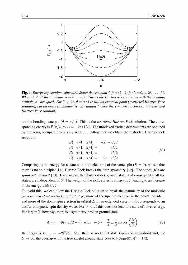
Fig. 4: Energy expectation value for a Slater determinant Φ(θ, π/2−θ) for U=0, t, 2t, . . . , 6t.When U ≤ 2t the minimum is at θ = π/4. This is the Hartree-Fock solution with the bondingorbitals ϕ+ occupied. For U ≥ 2t, θ = π/4 is still an extremal point (restricted Hartree-Focksolution), but an energy minimum is only attained when the symmetry is broken (unrestrictedHartree-Fock solution).

are the bonding state ϕ+ (θ = π/4). This is the restricted Hartree-Fock solution. The corre-sponding energy isE(π/4, π/4) = −2t+U/2. The unrelaxed excited determinants are obtainedby replacing occupied orbitals ϕ+ with ϕ−. Altogether we obtain the restricted Hartree-Fockspectrum

E( π/4, π/4) = −2t+ U/2

E( π/4,−π/4) = U/2

E(−π/4, π/4) = U/2

E(−π/4,−π/4) = 2t+ U/2

(87)

Comparing to the energy for a state with both electrons of the same spin (E = 0), we see thatthere is no spin-triplet, i.e., Hartree-Fock breaks the spin symmetry [12]. The states (87) arespin-contaminated [13]. Even worse, the Hartree-Fock ground state, and consequently all thestates, are independent of U . The weight of the ionic states is always 1/2, leading to an increaseof the energy with U/2.To avoid this, we can allow the Hartree-Fock solution to break the symmetry of the molecule(unrestricted Hartree-Fock), putting, e.g., more of the up-spin electron in the orbital on site 1and more of the down-spin electron in orbital 2. In an extended system this corresponds to anantiferromagnetic spin-density wave. For U < 2t this does not lead to a state of lower energy.For larger U , however, there is a symmetry-broken ground state

ΦUHF = Φ(θ, π/2− θ) with θ(U) =π

4± 1

2arccos

(2t

U

). (88)

Its energy is EUHF = −2t2/U . Still there is no triplet state (spin contamination) and, forU →∞, the overlap with the true singlet ground state goes to |〈ΦUHF|Ψ−〉|2 = 1/2.

Hartree-Fock and BCS 2.25

From Fig. 4 it might appear that there are just two degenerate unrestricted Hartree-Fock deter-minants. But, remembering that we can chose the spin quantization axis at will, we see that byrotating the spins by an angle α about the axis n (see App. C)

Rn(α) = e−in·~σ α/2 = cos(α/2)− i sin(α/2) n · ~σ

we can produce a continuum of degenerate solutions Rn(α)|ΦUHF〉. As an example we considerthe state we obtain when we rotate the spin quantization axis from the z into the x direction

Ry(−π/2) =1√2

(1 1

−1 1

)which transforms the creation operators according to (16) as(

c†i↑, c†i↓

)Ry(−π/2) =

(1√2

(c†i↑ − c

†i↓

),

1√2

(c†i↑ + c†i↓

)).

The determinant (85) thus transforms to

Ry(−π/2)|Φ(θ↑, θ↓)〉 =1

2

(s↓(c

†1↑ + c†1↓) + c↓(c

†2↑ + c†2↓)

)(s↑(c

†1↑ − c

†1↓) + c↑(c

†2↑ − c

†2↓))|0〉(89)

where we introduced the abbreviations sσ = sin θσ and cσ = cos θσ. Since the Hamiltonian (76)is invariant under spin rotations, Ry(−π/2) H R†y(−π/2) = H , the energy expectation value ofthe rotated state is still given by (86).

Attractive Hubbard model For negative U allowing the spin orbitals to differ, Φ(θ, π/2−θ),does lower the energy expectation value. The minimum is always obtained for the restrictedHartree-Fock determinant Φ(π/4, π/4). In fact, for the attractive Hubbard model rather thanbreaking spin symmetry, we should try to break the charge symmetry: For U < −2t the ansatzΦ(θ, θ) minimizes the energy for the two states θ(U) = π/4 ± arccos(−2t/U) with energyE(U) = 2t2/U + U . Thus, the unrestricted Hartree-Fock ground state breaks the charge sym-metry, i.e., is a charge-density wave state. On the other hand, looking back to (89) we seethat Φ(θ, θ) is invariant under the spin rotation. This is actually true for any Rn(α) so thatthe unrestricted Hartree-Fock ground state of the attractive Hubbard model does not break spinsymmetry.It seems strange that for the attractive model we only find two unrestricted Hartree-Fock states,while for the repulsive model we have a continuum of states. To find the ’missing’ states weconsider a new kind of transformation that mixes creation and annihilation operators: When weexchange the role of the creation and annihilation operators for the up spins only, i.e.,

c†i↑ = (−1)ici↑ and c†i↓ → c†i↓, (90)

the Hamiltonian (76) transforms into a two-site Hubbard model with the sign of U changed

H = −t∑σ

(c†2σ c1σ + c†1σ c2σ

)− U

∑i∈{1,2}

ni↑ni↓ + U(n1↓ + n2↓) . (91)

2.26 Erik Koch

Let us see what happens to the Slater determinant (85) when we apply the same transformation.In doing this, we have to remember that the vacuum state must vanish when acted on with anannihilator. For |0〉 this is no longer true for the transformed operators, but we can easily writedown a state

|0〉 = c†2↑c†1↑|0〉 (92)

that behaves as a suitable vacuum state: ciσ|0〉 = 0 and 〈0|0〉. We can then rewrite the trans-formed Slater determinant (85) as

|Φ(θ↑, θ↓)〉 =(

sin(θ↓) c†1↓ + cos(θ↓) c

†2↓

)(sin(θ↑) c

†1↑ + cos(θ↑) c

†2↑

)|0〉

=(

sin(θ↓) c†1↓ + cos(θ↓) c

†2↓

)(− sin(θ↑) c1↑ + cos(θ↑) c2↑

)c†2↑c

†1↑|0〉

=(

sin(θ↓) c†1↓ + cos(θ↓) c

†2↓

)(+ sin(θ↑) c

†2↑ + cos(θ↑) c

†1↑

)|0〉 .

Thus, the transformation takes the unrestricted state |Φ(θ, π/2 − θ)〉 for the repulsive Hubbardmodel into the unrestricted state |Φ(θ, θ)〉 for the attractive Hubbard model. Transforming therotated state (89) in the same way, we find something remarkable:

1

2

(s↓(c

†1↑ + c†1↓) + c↓(c

†2↑ + c†2↓)

)(s↑(c

†1↑ − c

†1↓) + c↑(c

†2↑ − c

†2↓))|0〉

=1

2

(s↓(−c1↑ + c†1↓) + c↓(c2↑ + c†2↓)

)(s↑(−c1↑ − c

†1↓) + c↑(c2↑ − c

†2↓))c†2↑c

†1↑|0〉

=1

2

((s↓c↑ + c↓s↑)

(c†1↓c

†1↑ + c†2↓c

†2↑)|0〉+ 2

(s↓s↑c

†1↓c†2↑ + c↓c↑c

†2↓c†2↑)|0〉

+ (s↓c↑ − c↓s↑)(c†2↓c

†1↓c†2↑c†1↑ − 1

)|0〉

).

The energy expectation value of this state is by construction the same as for the charge-densitystate. For θ↓ = π/2−θ↑ the new state has a uniform density, but the wave function no longer hasa well-defined particle number, i.e., it breaks particle number conservation. It is still a productstate in the transformed operators and vacuum, but it is a state in Fock space. States of this typeare crucial for describing superconductivity.

3.3 BCS theory

Next we consider the BCS Hamiltonian

HBCS =∑kσ

εk c†kσckσ −

∑kk′

Gkk′ c†k↑c†−k↓c−k′↓ck′↑ (93)

with an attractive interaction between pairs of electrons of opposite spin and momentum (Cooperpairs). We now want to see if we can use the idea of product states in Fock space that we encoun-tered for the attractive Hubbard model. To start, let us consider the determinant of plane wavestates that we used for the homogeneous electron gas |ΦkF 〉. Since all states with momentumbelow kF are occupied, we have

c†kσ|ΦkF 〉 = 0 for |k| < kF and ckσ|ΦkF 〉 = 0 otherwise.

Hartree-Fock and BCS 2.27

Thus |ΦkF 〉 behaves like a vacuum state for the transformed operators

ckσ = Θ(kF − |k|) c†kσ +Θ(|k| − kF ) ckσ =

{c†kσ for |k| < kFckσ for |k| > kF

Allowing the operators to mix, we can generalize this transformation to

bk↑ = ukck↑ − vkc†−k↓

bk↓ = ukck↓ + vkc†−k↑

The corresponding creation operators are obtained, of course, by taking the adjoint. Noticehow states with k and −k are mixed. These Bogoliubov-Valatin operators fulfill the canonicalanticommutation relations

{bkσ, bk′σ′} = 0 = {b†kσ, b†k′σ′} and {bkσ, bk′σ′} = δ(k − k′) δσ,σ′

when (the non-trivial anticommutators are {bk↑, b−k↓} and {bkσ, b†kσ})

u2k + v2

k = 1 . (94)

A vacuum state for the new operators can be constructed from the generalized product state∏kσ bkσ|0〉. Expanding the operators

b−k↑bk↓bk↑b−k↓|0〉 = vk(uk + vk c†−k↑c

†k↓) vk(uk + vk c

†k↑c†−k↓) |0〉

and calculating the norm

〈0|(uk + vk c−k↓ck↑)(uk + vk c†k↓c†−k↑)(uk + vk c

†−k↑c

†k↓)(uk + vk c

†k↑c†−k↓)|0〉 = u4

k + 2u2kv

2k + v4

k

we see from (94) that the BCS wavefunction

|BCS〉 =∏k

(uk + vk c†k↑c†−k↓) |0〉 (95)

is the (normalized) vacuum for the Bogoliubov-Valatin operators.To calculate physical expectation values we express the electron operators as

ck↑ = ukbk↑ + vkb†−k↓

ck↓ = ukbk↓ − vkb†−k↑

The expectation value for the occupation of a plane wave state, e.g., is

〈BCS|nk↑|BCS〉 = 〈BCS|(ukb†k↑+ vkb−k↓)(ukbk↑+ vkb†−k↓)|BCS〉 = v2

k = 〈BCS|n−k↓|BCS〉 .

Unlike the electron gas Slater determinant |ΦkF 〉, where nkσ is 1 below kF and vanishes above,varying the parameter vk in the BCS wave function allows us to get arbitrary momentum dis-tributions 〈nkσ〉. Since the BCS wave function has contributions in all particle sectors with aneven number of electrons, there are also less-conventional expectation values, e.g.,

〈BCS|c†k↑c†−k↓|BCS〉 = 〈BCS|(ukb†k↑ + vkb−k↓)(ukb

†−k↓ − vkbk,↑)|BCS〉 = ukvk = 〈c−k↓ck↑〉.

2.28 Erik Koch

When minimizing the energy expectation value, we have to introduce a chemical potential µthat is chosen to give the desired number of particles N =

∑kσ v

2k. We get

〈BCS|H − µN |BCS〉 =∑kσ

(εk − µ) v2k −

∑k,k′

Gkk′ ukvkuk′vk′ . (96)

Minimizing with respect to vk (and remembering that uk =√

1− v2k) we find the variational

equations

4(εk − µ) vk = 2∑k′

Gkk′

(uk −

vkukvk

)uk′vk′ . (97)

For simplicity we assume that Gkk′ is constant over a small range of k values around the Fermisurface and vanishes outside. We define

∆ :=∑k′

Gkk′ uk′vk′ = G∑

k:close to FS

ukvk (98)

and obtain, squaring the variational equation and remembering that 1− (u2k + v2

k)2 = 0,

4(εk − µ)2u2kv

2k = (εk − µ)2

(1− (u2

k − v2k)

2)

= ∆2(u2k − v2

k)

from which we get the momentum distribution

v2k =

1

2

(1− εk − µ√

(εk − µ)2 +∆2

). (99)

For∆ = 0 this is just the step function of a Fermi gas, for finite∆ the transition is more smooth.We still have to determine the parameters µ and ∆. The chemical potential is fixed by

N =∑k

2v2k =

∑k

(1− εk − µ√

(εk − µ)2 +∆2

)(100)

while for∆we obtain from (98), solving (97) for ukvk and summing over k, and using u2k−v2

k =

1− 2v2k

∆ = G∑k

ukvk =G

2

∑k

∆(u2k − v2

k)

εk − µ= ∆

G

2

∑k

1√(εk − µ)2 +∆2

(101)

the self-consistent gap equation for ∆.To see that ∆ is indeed a gap, consider the (unrelaxed) quasi-electron states

|k ↑〉 =1

ukc†k↑|BCS〉 = b†k↑|BCS〉. (102)

Adding an electron of momentum k destroys its Cooper pair, changing 〈nk↑+nk↓〉 from 2v2k to

1 and removing the interaction of the pair with all others:

〈k ↑ |H − µN |k ↑〉 − 〈BCS|H − µN |BCS〉 = (εk − µ) (1− 2v2k) + 2∆ukvk

= (εk − µ) (1− 2v2k) +

∆2

εk − µ(u2

k − v2k) = sgn(εk − µ)

√(εk − µ)2 +∆2.

For ∆ = we recover Koopmans’ Hartree-Fock result, while for ∆ > 0 a gap opens around theFermi level. Fig. 5 compares the quasi-electron dispersion and the corresponding density ofstates for the two cases.

Hartree-Fock and BCS 2.29

-1

-0.5

0

0.5

1

1.5

2

0 0.5 1 1.5

ε k - ε k

F

k/kF

∆=0∆=0.1

0 5 10 15 20 25 30density of states

∆=0∆=0.1

Fig. 5: Quasi-electron energy and density of states for the BCS state with and without gap.

4 Conclusion

We have seen that second quantization is an remarkable useful formalism. With just a few sim-ple rules for the creation and annihilation operators and the corresponding vacuum, it convertsdealing with many-electron states to straightforward algebraic manipulations. Moreover it isnaturally suited for performing calculations in variational spaces spanned by a finite basis of or-bitals. But its advantages go beyond a mere simplification. By abstracting from the coordinaterepresentation, it allows us to express many-body operators in a way that is independent of thenumber of electrons. Because of this it becomes possible to consider Fock-space wave func-tions which do not have a definite number of electrons. This allows us to consider unrestrictedmean-field states that not only break spatial or spin symmetries but also particle conservation.This additional freedom allows us to extend the concept of a Slater determinant to product statesin Fock space, an example of which is the BCS wave function.

Acknowledgment

Support of the Deutsche Forschungsgemeinschaft through FOR1346 is gratefully acknowledged.

2.30 Erik Koch

A Basis orthonormalization

A general one-electron basis spanned by functions |χn〉 will have an overlap matrix

Snm = 〈χn|χm〉

that is positive definite (and hence invertible) and hermitian. The completeness relation is

1 =∑k,l

|χk〉(S−1)kl〈χl| .

While we can work directly with such a basis, it is often more convenient to have an orthonormalbasis, so that we do not have to deal with the overlap matrices in the definition of the secondquantized operators and in the generalized eigenvalue problem.To orthonormalize the basis {|χn〉}, we need to find a basis transformation T such that

|ϕn〉 :=∑m

|χm〉Tmn with 〈ϕn|ϕm〉 = δmn .

This implies that T †ST = 1, or equivalently S−1 = TT †. This condition does not uniquelydetermine T . In fact there are many orthonormalization techniques, e.g., Gram-Schmidt or-thonormalization or Cholesky decomposition.Usually we will have chosen the basis functions |χn〉 for a physical reason, e.g., atomic orbitals,so that we would like the orthonormal basis functions to be as close to the original basis aspossible, i.e, we ask for the basis transformation T that minimizes∑

n

∣∣∣∣ |ϕn〉 − |χn〉 ∣∣∣∣2 =∑n

∣∣∣∣∣∣∑m

|χm〉(Tmn − δmn)∣∣∣∣∣∣2

= Tr (T † − 1)S (T − 1)

= Tr (T †ST︸ ︷︷ ︸=1

−T †S − ST + S) .

Given an orthonormalization T , we can obtain any other orthonormalization T by performinga unitary transformation, i.e., T = TU . Writing U = exp(iλM), we obtain the variationalcondition

0!

= Tr (+iMT †S − iSTM) = iTr (T †S − ST )M ,

which is fulfilled for ST = T †S, i.e., ST 2 = T †ST = 1. The second variation at T = S−1/2

1

2Tr (M 2S1/2 + S1/2M 2) > 0

is positive, since S and the square of the hermitian matrix M are both positive definite. Hencethe Lowdin symmetric orthogonalization [14]

TLowdin = S−1/2

minimizes the modification of the basis vectors.

Hartree-Fock and BCS 2.31

B Some useful commutation relations

Expression of commutators of products of operators can be derived by adding and subtractingterms that differ only in the position of one operator, e.g.,

[A1A2 · · ·AN , B] = A1A2 · · ·ANB −BA1A2 · · ·AN= A1A2 · · ·ANB − A1A2 · · ·BAN

+ A1A2 · · ·BAN − A1 · · ·BAN−1AN

+ · · ·+ A1BA2 · · ·AN −BA1A2 · · ·AN

=∑i

A1 · · ·Ai−1 [Ai, B] Ai+1 · · ·AN

The following special cases are particularly useful

[AB, C] = A [B, C] + [A, C]B

= A{B, C} − {A, C}B

[A, BC] = B [A, C] + [A, B]C

= [A, B]C + B [A, C]

= {A, B}C −B{A, C}

[AB, CD] = A [B, C]D + AC [B, D] + [A,C] DB + C [A, D]B

= A{B, C}D − AC{B, D}+ {A,C}DB − C{A, D}B

Important examples are [c†icj, c

†γ

]= c†iδj,γ[

c†icj, cγ

]= −cjδi,γ

For the commutator of products of creation and annihilation operators appearing in one- andtwo-body operators we find[

c†icj, c†αcβ

]=[c†icj, c

†α

]cβ + c†α

[c†icj, cβ

]= 〈j|α〉 c†icβ − 〈β|i〉 c

†αcj

and [c†ic†jckcl , c

†αcβ

]= 〈l|α〉 c†ic

†jckcβ + 〈k|α〉 c†ic

†jcβcl − 〈β|j〉 c

†ic†αckcl − 〈β|i〉 c

†αc†jckcl

2.32 Erik Koch

C Pauli matrices and spin rotations

The Pauli or spin matrices are defined as

σx =

(0 1

1 0

)σy =

(0 −ii 0

)σz =

(1 0

0 −1

)

They are hermitian, i.e. σ†i = σi , and σ2i = 1. Therefore their eigenvalues are ±1. The

eigenvectors of σz are |mz〉, mz = ±1:

|+ 1〉 =

(1

0

)and | − 1〉 =

(0

1

).

For these vectors we find

σx|mz〉 = | −mz〉 σy|mz〉 = imz| −mz〉 σz|mz〉 = mz|mz〉.

The products of the Pauli matrices are σx σy = iσz, where the indices can be permuted cycli-cally. From this follows for the commutator

[σx, σy] = 2iσz

while the anticommutator vanishes:{σx, σy} = 0

Finally a rotation by an angle α about the axis n changes the spin matrices

Rn(α) = e−in·~σ α/2 = cos(α/2)− i sin(α/2) n · ~σ .

Hartree-Fock and BCS 2.33

References

[1] P. Forrest: The Identity of Indiscernibles, in The Stanford Encyclopedia of Philosophy(Winter 2012 Ed.), E.N. Zalta (ed.)http://plato.stanford.edu/entries/identity-indiscernible/

[2] W. Pauli: The connection between spin and statistics, Phys. Rev. 58, 715 (1940)

[3] R.F. Streater and A.S. Wightman: PCT, Spin and Statistics, and All That(Benjamin, New York, 1964)

[4] P.-O. Lowdin: Quantum Theory of Many-Particle Systems I, Phys. Rev. 97, 1474 (1955)

[5] P. Jordan and O. Klein: Zum Mehrkorperproblem in der Quantenmechanik,Z. Physik 45, 751 (1927)

[6] P. Jordan and E. Wigner: Uber das Paulische Aquivalenzverbot, Z. Physik 47, 631 (1928)

[7] P. Jorgensen and J. Simons: Second Quantization-Based Methods in Quantum Chemistry(Academic Press, New York, 1981)

[8] D.J. Thouless: Stability conditions and nuclear rotations in the Hartree-Fock theory, Nucl.Phys. 21, 225 (1960)

[9] Le Thi Hoai: Product wave-functions in Fock-space(MSc Thesis, German Research School for Simulation Sciences, 2015)

[10] E. Koch: Many-Electron States in [15]

[11] S. Zhang and D.M. Ceperley: Hartree-Fock Ground State of the Three-DimensionalElectron Gas, Phys. Rev. Lett. 100, 236404 (2008)

[12] E. Koch: Exchange Mechanisms in [16]

[13] A. Szabo and N.S. Ostlund: Modern Quantum Chemistry (McGraw Hill, New York, 1989)

[14] P.-O. Lowdin: On the Non-Orthogonality Problem Connected with the Use of AtomicWave Functions in the Theory of Molecules and Crystals, J. Chem. Phys. 18, 365 (1950)

[15] E. Pavarini, E. Koch, and U. Schollwock (Eds.):Emergent Phenomena in Correlated Matter,Reihe Modeling and Simulation, Vol. 3 (Forschungszentrum Julich, 2013)http://www.cond-mat.de/events/correl13

[16] E. Pavarini, E. Koch, F. Anders, and M. Jarrell (Eds.): From Models to Materials,Reihe Modeling and Simulation, Vol. 2 (Forschungszentrum Julich, 2012)http://www.cond-mat.de/events/correl12