Scientific Annals of Computer Science vol.XX, 20XX

“Alexandru Ioan Cuza” University of Iasi, Romania

Symbolic Synthesis of Mealy Machines fromArithmetic Bitstream Functions

Helle Hvid HANSEN1 and Jan RUTTEN2

Abstract

In this paper, we describe a symbolic synthesis method which givenan algebraic expression that specifies a bitstream function f , con-structs a (minimal) Mealy machine that realises f . The synthesisalgorithm can be seen as an analogue of Brzozowski’s construction ofa finite deterministic automaton from a regular expression. It is basedon a coinductive characterisation of the operators of 2-adic arithmeticin terms of stream differential equations.

1 Introduction

A (binary) Mealy machine is a deterministic automaton which in each stepreads an input bit, produces an output bit and moves to a next state. Theinduced mapping of input streams to output streams is a causal bitstreamfunction, which we call the bitstream function realised by the Mealy ma-chine. In this paper, we describe a symbolic synthesis method which givenan algebraic expression that specifies a bitstream function f , constructs aminimal Mealy machine that realises f .

The inputs to our synthesis algorithm are called function expressionsand they define bitstream functions in the algebra of 2-adic numbers. Herewe use that the formal power series representation of a 2-adic integer canbe seen as the bitstream of its coefficients. We describe the 2-adic algebra

1Technische Universiteit Eindhoven and Centrum Wiskunde & Informatica, P.O.Box513, 5600 MB Eindhoven, The Netherlands, email: h.h.hansen@tue.nl.

2Centrum Wiskunde & Informatica and Radboud University Nijmegen, P.O.Box 94079,1090 GB Amsterdam, The Netherlands, email: janr@cwi.nl.

1

below, but for now such a function expression can be thought of as a spec-ification of a function on the rational numbers. The interesting property of2-adic arithmetic is that it allows us to calculate with bitstream represen-tations of rational numbers in an easy manner similar to how one computeswith integers.

The synthesis algorithm described here can be seen as an analogue ofBrzozowski’s construction in [3] of a finite deterministic automaton from aregular expression. In particular, we show that the set of function expres-sions carries the structure of a Mealy machine by giving an inductive defini-tion of derivative and output of function expressions. This Mealy machineof expressions is defined in such a way that the algebraic semantics coincideswith the behavioural semantics of Mealy machines, which will be defined interms of causal stream functions. Now given a function expression F speci-fying a function f , we obtain a realisation of f by the symbolic computationof the (sub)machine generated by F. (The generated submachine is in gen-eral not minimal, but we can ensure minimality by reducing expressions tonormal form.) The language of 2-adic arithmetic allows the specificationof functions that cannot be realised by any finite Mealy machine. But weshall identify a subclass of so-called rational function expressions for whicha finite realisation exists.

In the design of digital hardware, Mealy machines specify the behaviourof sequential circuits, and there exist algorithms which construct from a(finite) Mealy machine, a sequential circuit which exhibits the specified be-haviour. Combining these algorithms with our synthesis algorithm we thusobtain a complete construction from algebraic specification to sequentialcircuit.

In summary, the main contributions of the present paper are: (1) Theelementary but useful observation that the set of all causal stream functionsconstitutes a final Mealy machine, which forms the basis for a behaviouralsemantics of Mealy machines in terms of their minimisation. (Althoughminimisation of Mealy automata is well known [4], its characterisation hereby means of finality is new.) (2) The insight that given a rational func-tion expression F, we can effectively construct by symbolic computation a(minimal) Mealy machine that realises the bitstream function specified by F.

The basis for the present synthesis algorithm was given in [18]. Theseideas were developed into a proper algorithm in [8] (for an implementa-tion, see [7]). Further results on complexity and size of realisations wereincluded in the first author’s PhD thesis [6, Ch. 3]. This paper contains a

2

short, but improved presentation of the basic results in the abovementionedwork. In particular, the presentation of the Mealy machine of expressions,the algebraic semantics of function expressions, and the proof that algebraicsemantics coincides with behavioural semantics for function expressions arenew with respect to [6, 8, 18]. Moreover, the synthesis algorithm and com-plexity analysis have been simplified by making use of particular propertiesof rational function expressions. Finally, we mention that the theory un-derlying the present work is essentially coalgebraic (cf. [15]), but we havedeliberately chosen for a presentation which does not require any familiaritywith coalgebra.

Structure of the paper : In Section 2 we give the basic definitions re-garding Mealy machines. In Section 3 we describe the 2-adic algebra ofbitstreams and define the function expressions which serve as our specifica-tion language. In Section 4 we show how function expressions can be turnedinto a Mealy machine, and in Section 5 we present the synthesis algorithmfor rational function expressions and analyse its time complexity. Finally,we discuss related and future work in Section 6.

2 Mealy Machines

We give the basic definitions on Mealy machines, streams and causal streamfunctions. We introduce the notion of stream function derivative and showhow it can be used to turn the set of causal stream functions into a finalMealy machine, thus providing a characterisation of minimal Mealy ma-chines.

Let A and B be arbitrary sets. A Mealy machine 〈S,m〉 with inputsin A and outputs in B consists of a set of states S and a transition function

m : S → (B × S)A

This function maps a state s0 ∈ S to a function m(s0) : A→ (B×S), whichproduces for every input a ∈ A a pair 〈b, s1〉, consisting of the output b andthe next state s1. We call a Mealy machine binary if inputs and outputsare taken from the set 2 = {0, 1}. We will write

sa|b //t iff m(s)(a) = 〈b, t〉.

For an arbitrary set A, we denote by Aω the set of streams over A, i.e.,Aω = {α | α : N → A}. An element α ∈ Aω will be denoted by α =

3

(α(0), α(1), α(2), . . .). The head and tail maps on streams are denoted byhd and tl , respectively, that is, for α ∈ Aω, hd(α) = α(0) and tl(α) =(α(1), α(2), α(3), . . .). Later, in the context of stream differential equations,we will also refer to hd(α) and tl(α) as the initial value and stream derivativeof α, respectively, and write α′ instead of tl(α). Moreover, for α ∈ Aω andn ∈ N, we write α�n for the finite prefix (α(0), . . . , α(n)).

We define the (input-output) behaviour of a state s0 in S = 〈S,m〉as the stream function behS(s0) : Aω → Bω which maps an input stream(a0, a1, a2, . . . ) ∈ Aω to the output stream (b0, b1, b2, . . . ) ∈ Bω given by theunique sequence of transitions

s0a0|b0 // s1

a1|b1 // · · · ak|bk // sk+1ak+1|bk+1// · · ·

If S is clear from the context, we will often leave out the subscript and simplywrite beh(s). We say that a state s in 〈S,m〉 realises a stream function f ifbeh(s) = f .

Example 1 The figure below shows an example of a binary Mealy machinewhich starting in state s0 counts the number of ones in the input modulo2. Formally, s0 realises the function f defined on input stream α ∈ 2ω byf(α)(n) =

∑ni=0 α(i) mod 2 for all n ∈ N.

S : // s0

1|1

77

0|0��

s1

1|0''

0|1

++ s2

1|1

gg

0|0

ss

Note that, for all α ∈ 2ω and n ∈ N, f(α)(n) is determined by α(0), . . . , α(n).

We call a stream function f : Aω → Bω causal if the n-th element ofthe output stream f(α) depends only on the first n elements of the inputstream. More formally, f is causal if for all n ≥ 0 and all α, β ∈ Aω:

α�n = β �n =⇒ f(α)(n) = f(β)(n).

It is straightforward to prove that for any Mealy machine 〈S,m〉 and anys ∈ S, beh(s) : Aω → Bω is causal. Let Γ denote the set of all causal streamfunctions, i.e.,

Γ = {f | f : Aω → Bω and f is causal }.

4

Next, we will define a function γ : Γ → (B × Γ)A such that 〈Γ, γ〉 is aMealy machine. For α ∈ Aω and a ∈ A, we denote by a : α the stream(a, α(0), α(1), α(2), . . .), and given f : Aω → Bω, we write f(a :−) for thestream function that maps α to f(a : α). Now let f ∈ Γ and a ∈ 2. Wedefine

f [a] := hd ◦ f(a :−) ∈ Aω → Bfa := tl ◦ f(a :−) ∈ Aω → Bω (1)

Since f is causal, it follows that also fa is causal (hence fa ∈ Γ), and thatf [a] is constant, hence f [a] can be considered an element of B. We call f [a]the initial output of f on input a, and fa is the stream function derivativeof f on input a. We define the transition function

γ : Γ→ (B × Γ)A by γ(f)(a) = 〈f [a], fa〉 for all f ∈ Γ, a ∈ A.

This gives us an (infinite) Mealy machine Γ = 〈Γ, γ〉 with transitions

fa|f [a] // fa

Next we characterise 〈Γ, γ〉 using the following notion. A homomorphismof Mealy machines from 〈S,m〉 to 〈S′,m′〉 is a function h : S → S′ thatpreserves transitions: if m(s)(a) = 〈b, t〉 then m′(h(s))(a) = 〈b, h(t)〉; inother words,

sa|b // t ⇒ h(s)

a|b // h(t)

Theorem 2 For any Mealy machine S = 〈S,m〉, the map behS : S → Γ isthe unique homomorphism from S to Γ. In other words, Γ is a final Mealymachine.

Proof: Let 〈S,m〉 be an arbitrary Mealy machine. We denote the outputand next state functions defined by m at state s ∈ S by os and ds, re-spectively, that is, m(s)(a) = 〈os(a), ds(a)〉. To see that beh : S → Γ is ahomomorphism, let s ∈ S, a ∈ A and α ∈ Aω be arbitrary. We have:

beh(s)[a] = hd(beh(s)(a :α)) = os(a),

and by letting s0 = ds(a) and si+1 = dsi(α(i)) for all i ≥ 0, we have

(beh(s)a)(α) = tl(beh(s)(a :α))= tl(os(a), os0(α(0)), os1(α(1)), . . .)= (os0(α(0)), os1(α(1)), . . .)= beh(ds(a))(α).

5

Hence beh(s)a = beh(ds(a)). The proof that beh : S → Γ is the uniquehomomorphism from S to Γ is left to the reader. 2

The universality of 〈Γ, γ〉 can be expressed in yet another way. Weneed the following notions. For a state s ∈ S of a Mealy machine 〈S,m〉, let

〈〈s〉〉 ⊆ S

denote the smallest subset that contains s and is closed under transitions(for any inputs). Clearly, 〈〈s〉〉 is also a submachine of 〈S,m〉, by takingas its transition function the restriction of m to the set 〈〈s〉〉. We call 〈〈s〉〉the submachine generated by s in 〈S,m〉. We call 〈〈s〉〉 a realisation of f , ifbehS(s) = f , i.e., s realises f (in S). We say that a Mealy machine 〈S,m〉 isminimal if beh : 〈S,m〉 → 〈Γ, γ〉 is injective. From the finality of Γ, we get:

Corollary 1 For all f ∈ Γ, 〈〈f〉〉 is a minimal realisation of f .

Proof: Follows from the fact that the inclusion map 〈〈f〉〉 → Γ is an injectivehomomorphism of Mealy machines. 2

The final Mealy machine Γ thus consists of all the behaviours that canbe realised by some Mealy machine, and we therefore refer to beh(s) as thebehavioural semantics of a state s.

For a causal stream function f : Aω → Bω, we use the following nota-tion for repeated stream function derivatives: for w ∈ A∗ and a ∈ A, wedefine fε = f (where ε is the empty word) and fwa = (fw)a. Hence the stateset of 〈〈f〉〉 equals the set {fw | w ∈ A∗} of all stream function derivatives off .

Example 3 We illustrate the notions and results above with the binarycounter from Example 1. Let f = beh(s0), g = beh(s1) and h = beh(s2). Itcan easily be seen that f = h and g(α)(k) = 1− f(α)(k) for all α ∈ 2ω andk ∈ N. Moreover, we have the following initial outputs and stream functionderivatives:

f [0] = 0, f [1] = 1, g[0] = 1, g[1] = 0, f0 = f, f1 = g, g0 = g, g1 = f

and thus beh maps S = 〈〈s0〉〉 to its minimisation 〈〈f〉〉 ⊆ Γ, on the right:

s0 1|1 88

0|0

++ s1

1|0&&

0|1

++ s2

1|1

ff

0|0

ss � beh // f

1|1$$

0|0

,, g

1|0

dd

0|1

qq

6

In algebra, the behaviour of Mealy machines is typically described interms of functions of type A+ → B. Although this set is isomorphic to Γ,we prefer to work with the latter because of the rich algebraic structure onstreams. The notion of stream function derivative already occurs in [13],and is called state there. It is also a variation on the classical notion ofderivative (or inverse) of functions from A∗ to B∗ (cf. [4]). Also Theorem 2and Corollary 1 are essentially reformulations of classical results.

The main contribution of the present paper consists of the observationthat 〈〈f〉〉 can often be constructed by a symbolic computation of streamfunction derivatives starting from an algebraic specification of f . In Sec-tion 5, we shall describe such a symbolic algorithm for bitstream functionsspecified in 2-adic arithmetic.

3 The 2-Adic Bitstream Algebra

We will specify bitstream functions in the algebra of 2-adic integers (cf. [5]).A 2-adic integer is usually written as a (formal) power series of the form∑∞

i=0 ai2i where ai ∈ 2 for all i ∈ {0, 1, 2, . . .}. We identify such a power

series with the bitstream (a0, a1, a2, . . .), so for us the set of 2-adic integersis simply the set 2ω of bitstreams.

There is a (strict) inclusion of the set of rational numbers with odddenominator

Qodd = {p/q | p, q ∈ Z, q odd }into the 2-adic integers by taking infinitary base 2 expansions (see e.g. [10]).For a positive integer n, this is just the binary representation of n (leastsignificant bit on the left) padded with a tail of zeros; for instance,

Bin(2) = (0, 1, 0, 0, 0, . . .) = 010ω

Bin(5) = (1, 0, 1, 0, 0, . . .) = 1010ω

Binary representations of negative integers end with an infinite sequence ofones and rational numbers (with odd denominator) have binary representa-tions that are eventually periodical; for instance,

Bin(−1) = (1, 1, 1, 1, . . .) = 1ω

Bin(−5) = (1, 1, 0, 1, 1, 1, . . .) = 1101ω

Bin(1/5) = (1, 0, 1, 1, 0, 0, 1, 1, 0, 0, 1, 1, 0, . . .) = 1(0110)ω.

(Rationals with even denominator require formal power series representa-tions

∑∞i=k ai2

i where k < 0, and are not treated here.)

7

Below we shall define the binary representation Bin(q) of any rationalq ∈ Qodd by means of a stream differential equation. Such equations specifystreams σ, in analogy with traditional differential calculus, in terms of theirinitial value σ(0) and derivative σ′ (which are defined as hd(σ) and tl(σ)).For instance, the differential equation

σ′ = σ σ(0) = 1

clearly defines the stream (1, 1, 1, . . .). We refer to [16] for an overview onstream differential equations.

Now let odd(n/2m + 1) = n mod 2 for n,m ∈ Z. We define theinclusion map

Bin : Qodd → 2ω

by the following system of stream differential equations (one for each q ∈Qodd ):

Bin(q)(0) = odd(q), Bin(q)′ = Bin((q − odd(q))/2) (2)

The reader is invited to compute the examples of binary expansions givenabove, using this definition of Bin.

We recall that the set of rational numbers (with odd denominator) isan integral domain: a commutative ring in which multiplication has no zero-divisors, i.e., for all p and q, if p× q = 0 then p = 0 or q = 0. Next we shallintroduce operations of addition and multiplication (as well as minus andinverse) on the set of 2-adic integers such that they reflect the operationson the rationals. More formally, we shall turn the set of 2-adic integers intoan integral domain

A2adic = 〈2ω, +, −, ×, /, [0], [1]〉

such that the inclusion map Bin : Qodd → 2ω is a homomorphism of integraldomains.

In the literature, the operators on the 2-adic integers are often definedby explicitly specifying how they work on binary representations, see Fig-ure 1 for examples of addition and multiplication. Their definitions aresometimes also given in terms of their representation as power series, typi-cally in the form of some recurrence relation on their coefficients. Here weshall give, instead, a definition by means of stream differential equations,which we saw already examples of above, and which can be seen as a gen-eralisation of definitions by recurrence, cf. [16]. Our choice to use streamdifferential equations is not just a matter of taste: they form the basis for

8

addition: 1 1 1 . . . (carry)1 0 1 0 0 0 · · · = 5

+ 0 1 1 1 1 1 · · · = −21 1 0 0 0 0 · · · = 3

multiplication: 1 1 0 0 0 · · · × 0 1 1 1 1 · · · = 3× (−2)0 0 0 0 0 0 · · ·

1 1 0 0 0 · · ·1 1 0 0 0 · · ·

1 1 0 0 0 · · ·1 1 0 0 0 · · ·

+...

0 1 0 1 1 1 · · · = −6

Figure 1: Examples of 2-adic addition and multiplication.

the definition of the Mealy machine of stream function expressions, to beintroduced in Section 4.

First we define the constants zero and one by

[0] = (0, 0, 0, . . .) [1] = (1, 0, 0, 0, . . .)

Below we shall use the following Boolean operators on 2 = {0, 1}, whichare defined, for all a, b ∈ 2, as usual: a ∧ b = min{a, b} and a ⊕ b = 1 iffa = 0, b = 1 or a = 1, b = 0 (exclusive or).

Definition 1 We define the operators of addition, minus, multiplicationand inverse of 2-adic integers by the following system of stream differentialequations. For α, β ∈ 2ω,

derivative: initial value:(α+ β)′ = (α′ + β′) + [α(0) ∧ β(0)] (α+ β)(0) = α(0)⊕ β(0)(−α)′ = −(α′ + [α(0)]) (−α)(0) = α(0)(α× β)′ = (α′ × β) + ([α(0)]× β′) (α× β)(0) = α(0) ∧ β(0)(1/α)′ = −(α′ × (1/α) ) (1/α)(0) = 1

There is a side condition for the definition of inverse: 1/α is defined onlyfor α with α(0) = 1.

9

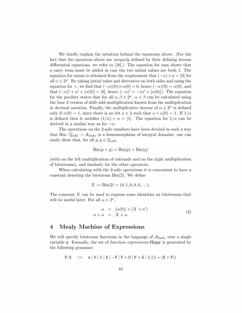
We briefly explain the intuition behind the equations above. (For thefact that the operators above are uniquely defined by their defining streamdifferential equations, we refer to [16].) The equation for sum shows thata carry term must be added in case the two initial values are both 1. Theequation for minus is obtained from the requirement that (−α)+α = [0] forall α ∈ 2ω. By taking initial value and derivative on both sides and using theequation for +, we find that (−α)(0)⊕α(0) = 0, hence (−α)(0) = α(0), andthat (−α)′ + α′ + [α(0)] = [0], hence (−α)′ = −(α′ + [α(0)]). The equationfor the product states that for all α, β ∈ 2ω, α × β can be calculated usingthe base 2 version of shift-add-multiplication known from the multiplicationin decimal notation. Finally, the multiplicative inverse of α ∈ 2ω is definedonly if α(0) = 1, since there is no bit a ∈ 2 such that a ∧ α(0) = 1. If 1/αis defined then it satisfies (1/α) × α = [1]. The equation for 1/α can bederived in a similar way as for −α.

The operations on the 2-adic numbers have been devised in such a waythat Bin: Qodd → A2adic is a homomorphism of integral domains: one caneasily show that, for all p, q ∈ Qodd ,

Bin(p× q) = Bin(p)× Bin(q)

(with on the left multiplication of rationals and on the right multiplicationof bitstreams), and similarly for the other operators.

When calculating with the 2-adic operations it is convenient to have aconstant denoting the bitstream Bin(2). We define

X := Bin(2) = (0, 1, 0, 0, 0, . . .),

The constant X can be used to express some identities on bitstreams thatwill be useful later: For all α ∈ 2ω,

α = [α(0)] + (X × α′)α+ α = X × α (3)

4 Mealy Machine of Expressions

We will specify bitstream functions in the language of A2adic over a singlevariable s. Formally, the set of function expressions FExpr is generated bythe following grammar:

F, G ::= s | 0 | 1 | X | −F | F + G | F× G | 1/(1 + (X× F))

10

We use the symbols −,+,×, / to denote the operations on bitstreams aswell as the corresponding syntax constructors. The typing should alwaysbe clear from the context. We will use standard notational conventions: wewrite Fn for the n-fold product of F with itself, (in particular, F0 = 1) andF/(1 + (X× G)) or F

1+(X×G) instead of F× (1/(1 + (X× G))). The algebraicsemantics of function expressions is given by the expected interpretation inA2adic . The reason we only allow division by terms of the form 1 + (X× F)is to ensure that the inverse operation is always defined when evaluatingfunction expressions in A2adic .

Definition 2 We define the algebraic 2-adic semantics [[F]] : 2ω → 2ω of afunction expression F ∈ FExpr by the following inductive clauses. Let σ bea bitstream,

[[s]](σ) = σ

[[0]](σ) = [0][[1]](σ) = [1][[X]](σ) = X

[[−F]](σ) = −([[F]](σ))[[F + G]](σ) = [[F]](σ) + [[G]](σ)[[F× G]](σ) = [[F]](σ)× [[G]](σ)

[[1/(1 + (X× F)]](σ) = 1/(1 + (X × [[F]](σ))

We say that a function expression F specifies the bitstream function[[F]], and two function expressions F and G are equivalent (notation: F ≡ G)if [[F]] = [[G]].

One easily shows (by structural induction on function expressions) thatfor all F ∈ FExpr, [[F]] is a causal bitstream function. In other words,[[−]] is a map from FExpr to Γ. We will now define a transition functionξ : FExpr → (2 × FExpr)2 such that 〈FExpr, ξ〉 is a binary Mealy machineand the algebraic semantics [[−]] : FExpr → Γ is a Mealy homomorphism.That is, for each F ∈ FExpr and a ∈ 2, we want to define F[a] ∈ 2 andFa ∈ FExpr such that F[a] = [[F]][a] and [[Fa]] = [[F]]a. In order to do so, firstrecall how we defined γ(f)(a) in terms of f(a :−), hd and tl (cf. equation(1)) for f ∈ Γ and a ∈ 2. We will “mimic” γ in the syntax.

First, we need a syntactic version of the map f(a :−) for f ∈ Γ anda ∈ 2. More precisely, given F ∈ FExpr and a ∈ 2, we want to find afunction expression which specifies [[F]](a : −). Note that for all σ ∈ 2ω,[[0 + (X× s)]](σ) = 0:σ and [[1 + (X× s)]](σ) = 1:σ.

Definition 3 We define ι : 2 → FExpr by ι(0) = 0 and ι(1) = 1, and forF ∈ FExpr and a ∈ 2, we let a :s := ι(a) + (X× s). We define F(a :s) to bethe function expression obtained by uniformly substituting a :s for s in F.

11

We now show that F(a :s) indeed specifies [[F]](a :−).

Lemma 1 For all F ∈ FExpr, all a ∈ 2 and all σ ∈ 2ω:

[[F(a :s)]](σ) = [[F]](a :σ).

Proof: The lemma is proved by a straightforward induction on the structureof F. We only show a few example cases:

[[s(a :s)]](σ) = [[ι(a) + (X× s)]](σ)

= [[ι(a)]](σ) + ([[X]](σ)× [[s]](σ))

= [a] + (X × σ)

(cf. eqn. (3)) = a :σ = [[s]](a :σ)

[[(F + G)(a :s))]](σ) = [[F(a :s) + G(a :s)]](σ)

= [[F(a :s)]](σ) + [[G(a :s)]](σ)IH= [[F]](a :σ) + [[G]](a :σ)

= [[F + G]](a :σ)

2

The transition function ξ on function expressions is defined inductivelyover the syntactic structure. In order to motivate the definition of ξ, con-sider, for example, a product expression F × G, and suppose that [[F]] = fand [[G]] = g. We then want [[(F × G)a]](σ) = tl(f(a : σ) × g(a : σ)) for allσ ∈ 2ω. By the stream differential equation for product, this means that

[[(F× G)a]](σ) = (tl(f(a :σ))× g(a :σ)) + ([hd(f(a :σ))]× tl(g(a :σ)))

= (fa(σ)× g(a :σ)) + ([f [a]]× ga(σ)

= ([[F]]a(σ)× [[G]](a :σ)) + ([[[F]][a]]× [[G]]a(σ).

Comparing this equation with the definition of (F× G)a below it is easy tosee that an induction argument and Lemma 1 will show that [[(F × G)a]] =[[F× G]]a.

12

Definition 4 Let ξ : FExpr→ (2× FExpr)2 be the map given by ξ(F)(a) =〈F[a], Fa〉 where F[a] and Fa are defined for all F ∈ FExpr and a ∈ 2 by:

syntactic initial outputs[a] = a (−F)[a] = F[a]0[a] = 0 (F + G)[a] = F[a]⊕ G[a]1[a] = 1 (F× G)[a] = F[a] ∧ G[a]X[a] = 0 (1/(1 + (X× F)))[a] = 1

syntactic stream function derivativesa = s (−F)a = −(Fa + ι(F[a]))0a = 0 (F + G)a = (Fa + Ga) + ι(F[a] ∧ G[a])1a = 0 (F× G)a = (Fa × G(a :s)) + (ι(F[a])× Ga)Xa = 1 (1/(1 + (X× F)))a = −(F(a :s))/(1 + (X× F(a :s)))

We call 〈FExpr, ξ〉 the Mealy machine of expressions, and we refer to F[a]and Fa as the syntactic initial output, respectively the syntactic stream func-tion derivative, of F on input a.

We now show that ξ indeed ensures that the algebraic semantics con-cides with the behavioural semantics of function expressions.

Proposition 1 The map [[−]] : FExpr → Γ is a homomorphism of Mealymachines from 〈FExpr, ξ〉 to 〈Γ, γ〉.

Proof: We must show that for all F ∈ FExpr and all a ∈ 2:

[[F]][a] = F[a] and [[Fa]] = [[F]]a.

The proof is by induction on the structure of F. We only show the casefor s and product; the others can be shown along the same lines (the fullproof details are found in the Appendix). In the identities below, IH refersto the induction hypothesis. Note also that for any b ∈ 2 and σ ∈ 2ω:[[ι(b)]](σ) = [b]. Let a ∈ 2 and σ ∈ 2ω.

[[s]][a] = ([[s]](a :σ))(0) = (a :σ)(0) = a = s[a].[[s]]a(σ) = ([[s]](a :σ))′ = (a :σ)′ = σ = [[sa]](σ).

[[F× G]][a] = ([[F× G]](a :σ))(0) = ([[F]](a :σ)× [[G]](a :σ))(0)= [[F]][a] ∧ [[G]][a]IH= F[a] ∧ G[a] = (F× G)[a].

13

[[F× G]]a(σ) = ([[F× G]](a :σ))′ = ([[F]](a :σ)× [[G]](a :σ))′

= (([[F]](a :σ))′ × [[G]](a :σ)) + ([([[F]](a :σ))(0)]× ([[G]](a :σ))′)= ([[F]]a(σ)× [[G]](a :σ)) + ([[[F]][a]]× [[G]]a(σ))IH= ([[Fa]](σ)× [[G]](a :σ)) + ([F[a]]× [[Ga]](σ))

Lem.1= [[(Fa(σ)× G(a :s)) + (ι(F[a])× Ga)]](σ)= [[(F× G)a]](σ).

2

Since 〈Γ, γ〉 is a final Mealy machine, the map [[−]] coincides with theunique homomorphism beh : 〈FExpr, ξ〉 → 〈Γ, γ〉. In other words, we haveshown that for all function expressions F, [[F]] = beh(F).

5 Synthesis

A consequence of Proposition 1 is that the generated submachine 〈〈F〉〉 isa realisation of [[F]]. Conceptually, we can construct 〈〈F〉〉 by computingthe transition closure of {F} in 〈FExpr, ξ〉. However, in general, 〈〈F〉〉 isneither finite nor minimal. In order to obtain a minimal realisation of [[F]] wecompute 〈〈F〉〉 modulo equivalence. In practice, this is achieved by reducingfunction expressions to normal form, which we briefly describe now.

5.1 Normal forms

We call a function expression F integral if it does not contain the inverseoperation, and F is closed if it does not contain s. The polynomial normalform pnf (F) of an integral expression F is an analogue of the distributednormal form of polynomials (in the variable s). It can be computed in theexpected manner by applying identities of commutative rings: (i) distribute× over +, (ii) reduce using identities for 0 and 1, (iii) collect terms on powersof s, and finally (iv) reduce sums of closed expressions using the identityXn + Xn = Xn+1, for all n ≥ 0. This last identity holds since for all α ∈ 2ω,α+α = X ×α, cf. equation (3). For example, pnf ((1 + X)× (1 + s) + 1) =X2 + (1 + X) × s, and this polynomial normal form is “computed” in the

14

following series of identities:

((1 + X)× (1 + s)) + 1 ≡ ((1 + X)× 1) + ((1 + X)× s) + 1≡ ((1× 1) + (X× 1)) + ((1× s) + (X× s)) + 1≡ (1 + X) + (s + (X× s)) + 1≡ (1 + 1 + X) + (1 + X)× s≡ X2 + (1 + X)× s.

Note that in the last step we used that,

1 + 1 + X ≡ X0 + X0 + X1 ≡ X1 + X1 ≡ X2.

For any integral expression F, it should be clear that F ≡ pnf (F) and thatpnf (F) is unique: pnf (F) = pnf (G) if and only if F ≡ G. Given arbitraryfunction expressions F and G, we can therefore decide whether F ≡ G by firstrewriting (using the identities of integral domains) F and G into fractionsP/Q and R/S, respectively, where P, Q, R, S are integral, and then checkingwhether pnf (P× S) = pnf (R× Q). These normal forms are treated in moredetail in [6]. In fact, in our synthesis algorithm we only need to computenormal forms of closed, integral expressions, as we will see in Section 5.3.

Example 4 We illustrate by computing (a representation of) 〈〈[[F]]〉〉 for thefunction expression F = (1 + X)× s. For the transition on input 1 we findthat:

((1 + X)× s)[1] = (1[1]⊕ X[1]) ∧ s[1] = (1⊕ 0) ∧ 1 = 1.

((1 + X)× s)1 = ((1 + X)1 × s(1 :s)) + (ι((1 + X)[1])× s1)= (((11 + X1) + ι(1[1] ∧ X[1]))× (1 + (X× s)))

+(ι(1[1]⊕ X[1])× s1)= ((0 + 1) + (ι(1 ∧ 0)× (1 + (X× s)))) + (ι(1⊕ 0)× s)= (((0 + 1) + 0)× (1 + (X× s)) + (1× s)≡ 1 + ((1 + X)× s) = 1 + F

Computing further derivatives and initial output, we find the followingminimal realisation of [[F]]:

// f

1|1$$

0|0��

f1

0|1

cc

1|0&&f11

0|0

ee

1|1��

where f = [[F]], f1 = [[1 + F]] and f11 = [[X + F]].

15

The normal forms essentially allow us to compute submachines in thefinal Mealy machine. Still, for arbitrary F ∈ FExpr, the least fixed pointconstruction of 〈〈[[F]]〉〉 is not guaranteed to terminate as it is easy to specifyfunctions that have no finite realisation. For example, if we take F = s× sand we compute the derivatives [[F]]0, [[F]]00, [[F]]000, . . . we get the sequence[[X × F]], [[X2 × F]], [[X3 × F]], . . . which are all distinct. A similar argumentshows that if F = 1/(1 + (X× s)), then [[F]] has infinitely many distinctstream function derivatives.

5.2 Rational functions

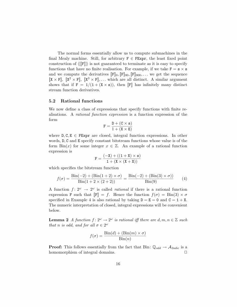
We now define a class of expressions that specify functions with finite re-alisations. A rational function expression is a function expression of theform

F =D + (C× s)1 + (X× E)

where D, C, E ∈ FExpr are closed, integral function expressions. In otherwords, D, C and E specify constant bitstream functions whose value is of theform Bin(x) for some integer x ∈ Z. An example of a rational functionexpression is

F =(−X) + ((1 + X)× s)1 + (X× (X + X))

which specifies the bitstream function

f(σ) =Bin(−2) + (Bin(1 + 2)× σ)

Bin(1 + 2× (2 + 2))=

Bin(−2) + (Bin(3)× σ))Bin(9)

(4)

A function f : 2ω → 2ω is called rational if there is a rational functionexpression F such that [[F]] = f . Hence the function f(σ) = Bin(3) × σspecified in Example 4 is also rational by taking D = E = 0 and C = 1 + X.The numeric interpretation of closed, integral expressions will be convenientbelow.

Lemma 2 A function f : 2ω → 2ω is rational iff there are d,m, n ∈ Z suchthat n is odd, and for all σ ∈ 2ω

f(σ) =Bin(d) + (Bin(m)× σ)

Bin(n)

Proof: This follows essentially from the fact that Bin: Qodd → A2adic is ahomomorphism of integral domains. 2

16

To simplify notation, we will leave out the Bin-part, and just writef(σ) = (d+ (m× σ))/n whenever f(σ) = (Bin(d) + (Bin(m)× σ)))/Bin(n).Similarly, for x ∈ Z, we write x(0) and x′ instead of Bin(x)(0) and Bin(x)′,respectively. The following technical lemmas will be used to prove thatrational functions have finite realisations. Their proofs can be found in theAppendix. The first of these lemmas uses the numeric interpretation ofrational functions to characterise the immediate derivatives.

Lemma 3 Let f be a rational bitstream function of the form:

f(σ) =d+ (m× σ)

n

for integers d,m and n with n odd. For a ∈ 2, the stream function derivativefa is given by:

(fa)(σ) =δ(a) + (m× σ)

n(5)

where (in the numeric interpretation)

δ(0) =

{12 d if d even12(d− n) if d odd

δ(1) =

{12(d+m) if d+m even12(d+m− n) if d+m odd

Hence Lemma 3 already tells us that the derivatives of a rational func-tion are again rational. The next lemma uses the numeric interpretation togive a bound on the range of δ-values that can occur in the stream functionderivatives of a rational function.

Lemma 4 Let f(σ) = d+(m×σ)n be a rational function with n > 0 odd. For

all w ∈ 2∗, the stream function derivative fw is of the form

(fw)(σ) =δ(w) + (m× σ)

n(6)

where δ(w) is an integer such that

min{d,−n+ 1,−n+m+ 1} ≤ δ(w) ≤ max{d,m− 1, 0}.

The crucial properties that make it possible to perform synthesis fromrational function specifications are stated in the following proposition.

17

Proposition 2 For all rational bitstream functions f : 2ω → 2ω,

1. all stream function derivatives of f are rational,

2. 〈〈f〉〉 is finite.

Proof: Let f(σ) = d+(m×σ)n be a rational function. Item 1 of the proposition

follows from Lemmas 2 and 3. To see that item 2 holds, first note that we canalways assume that n > 0 since f is equal to the function g(σ) = −d+(−m×σ)

−n .The number of states in 〈〈f〉〉 equals the number of distinct δ(w)-values inthe derivatives of f . By Lemma 4 this number is finite. 2

5.3 Algorithm

We construct 〈〈[[F]]〉〉 for a rational function expression F by computing statesand transitions in the final Mealy machine. Stream function derivatives of[[F]] are denoted by rational function expressions, and in order to efficientlydetermine when two expressions denote the same derivative, we normalisethe closed integral subexpressions of F at the beginning of the computation.More precisely, if F = (D + (C × s))/(1 + (X × E)) is a rational functionexpression, then we define the reduced form of F as

red(F) = (pnf (D) + (pnf (C)× s))/(1 + (X× pnf (E))),

and we call F reduced, if F = red(F). Starting from a reduced expression,all derivatives computed during the synthesis algorithm are represented ina similar, reduced form. This is achieved by using the function next.

Definition 5 Given a rational function expression

F =D + (C× s)1 + (X× E)

we define

nextD(F, 0) = D0 +−(D[0]× E), andnextD(F, 1) = ((D1 + C1) + ι(D[1] ∧ C[1])) +−(ι(D[1]⊕ C[1])× E),

and for a ∈ 2 we define

next(F, a) =pnf (nextD(F, a)) + (C× s)

1 + (X× E).

18

It should be clear that starting from a reduced function expressionF, any two expressions computed with the next-function are equivalent ifand only if they are (syntactically) equal. The next lemma shows that thenext-function can be identified with the syntactic derivative function.

Lemma 5 For all rational function expressions F and all a ∈ 2,

next(F, a) ≡ Fa.

Proof: The lemma follows easily by writing out the details of the definitionof Fa, and applying integral domain identities. See also the proof of Lemma 3(in the Appendix). 2

The synthesis algorithm is shown in Figure 2 (and we explain it in somemore detail below). We denote the empty list by [ ], the concatenation oftwo lists x and y by x.y, and we let remdup be a function that removesduplicates from a list. If S is a list of states (i.e. reduced rational functionexpressions) and T is a list of transitions, then transitions(S) is the listof transitions with source state in S, and targets(T ) is the list of targetstates of transitions in T . Using list comprehension, we can write this moreprecisely as:

transitions(S) := [ G 0|G[0]→ next(G, 0), G 1|G[1]→ next(G, 1)) | G ∈ S ],

targets(T ) := [ G | G a|b→ H ∈ T ];

1. NewStates := [ red(F) ]; States := [ ]; Trans := [ ];2. do until NewStates = ∅ {3. NewTrans := transitions(NewStates);4. Trans := Trans.NewTrans;5. States := States.NewStates;6. NewStates := remdup(targets(NewTrans)) \ States;7. }8. return Trans;

Figure 2: Synthesis algorithm

The synthesis algorithm is a standard least fixed point algorithm. Werepresent a (partially constructed) Mealy machine as a list Trans of tran-sitions. A list States is also used to keep track of which states have been

19

processed, and a list NewStates contains the states that were newly foundin the previous iteration. Initially, NewStates only contains the initial spec-ification in reduced form. In each iteration, we compute the list NewTransof transitions starting from NewStates, and add these to Trans. The newstates for the next iteration are the target states of NewTrans except forthe ones that have already been processed. At the end of iteration numberk, all states and transitions up to depth k have been created. Hence whenno new states are found, Trans represents 〈〈[[F]]〉〉.

We can now finally state our synthesis result for rational function spec-ifications.

Theorem 5 For any rational function expression F, we can effectively con-struct a finite, minimal realisation of [[F]] using the algorithm in Figure 2.

Proof: By Corollary 1 and Proposition 2, 〈〈[[F]]〉〉 is a finite, minimal re-alisation of [[F]]. The algorithm in Figure 2 constructs a Mealy machine〈S,m〉 whose states are (rational) function expressions. Due to Lemma 5,and the fact that all rational function expressions in S are reduced and havethe same “denominator” expression, two function expressions s1, s2 ∈ S areequivalent if and only if they are (syntactically) identical. Hence 〈S,m〉 isminimal. 2

We illustrate our synthesis algorithm with a couple of examples.

Example 6 We construct the minimal realisation of the function f speci-fied by F = X3 × s, i.e., in numeric notation, f(σ) = 8×σ for all σ ∈ 2ω. Forthe sake of readability, we will write derivative expressions in their numericinterpretation. For example, the derivative (X2 + (X3 × s)) will be denoted4 + 8σ. The diagram in Figure 3 shows the Mealy machine obtained fromF using our algorithm. At the beginning of the computation, the only stateis 8σ. In the first iteration, the immediate derivatives of 8σ are computed.These are 8σ and 4 + 8σ, so 4 + 8σ is a new state. In the second iteration,we compute the immediate derivatives of 4 + 8σ and find 2 + 8σ and 6 + 8σ,both of which are new. In the third iteration, we find the new states 1+8σ,5+8σ, 3+8σ and 7+8σ. In the fourth iteration, we find that all derivativesof the states 1+8σ, 5+8σ, 3+8σ and 7+8σ have already been visited, hencethere are no new states after this round, and the algorithm terminates.

20

1 + 8σ

0|1

��

1|1

��

2 + 8σ1|0 //

0|0 44iiiiiiiiiiii5 + 8σ

0|1

hh

1|1

yysssssssssssssssss

8σ

0|0

�� 1|0 // 4 + 8σ0|0

66nnnnnnn

1|0((PPPPPPPOO

6 + 8σ0|0 //

1|0 **UUUUUUUUUUUU 3 + 8σ

1|1

OO0|1

aa

7 + 8σ0|1

OO

1|1

XX

Figure 3: Mealy machine constructed from F = X3 × s.

Example 7 As yet another example, in Figure 4 we give a minimal realisa-tion of the rational function from equation (4), i.e., f(σ) = ((−2)+(3×σ))/9.For a compact presentation, the states are labelled only by the δ-value. Forexample, the state which realises the function (1+(3×σ))/9 is labelled justwith 1.

1

1|0

��

0|1 // −4

0|0

��

1|1

��

−8

1|1

��

0|0oo

−5

1|0&&

0|1xxqqqqqqqqq −1

0|1

ff

1|0

{{

2

0|0

HH

1|1 // −2

1|1

HH

0|1

@@

−7

0|1

HH

1|0ooOO

Figure 4: Mealy machine realising f(σ) = ((−2) + (3× σ))/9.

21

Knowing that rational functions have finite realisations, it is naturalto ask whether the converse holds, that is, whether all causal bitstreamfunctions that are realised by a finite Mealy machine can be specified by arational function expression. This question is answered in the negative bythe following example.

Example 8 Consider the Mealy machine depicted in the following diagram:

q

0|1

�� 1|1 // s

0|0,1|1

��

We will show that there is no rational function expression F such that [[F]] =beh(q). To this end, we first observe that the behaviour of the state s issimply the identity function on bitstreams, hence beh(s) = [[s]]. Suppose, forthe sake of arriving at a contradiction, that F is a function expression suchthat [[F]] = beh(q), and F is of the form F = (B + (C× s))/(1 + (X× E)) whereB, C, E ∈ FExpr are closed, integral function expressions. By Proposition 1,[[F0]] = [[F]]0 = beh(q)0 = beh(s) = [[s]], hence F0 ≡ s. On the other hand,Lemma 3 tells us that F0 ≡ (D + (C× s))/(1 + (X× E)) for some closed,integral function expression D, and hence (D + (C× s))/(1 + (X× E)) ≡ s.Consequently, D ≡ 0, C ≡ 1 + (X× E), which implies that C[0] = C[1] = 1.From Definition 4 of the Mealy machine of expressions it follows that for alla ∈ 2:

F[a] = (B + (C× s))[a] = B[a]⊕ (C[a] ∧ s[a]) = B[a]⊕ (1 ∧ a)

= B[a]⊕ a,

and hence,F[0] = B[0] and F[1] = 1− B[1]

But since B is a closed function expression, B[0] = B[1], and hence by theabove F[0] 6= F[1]. But beh(q)[0] = beh(q)[1] = 1 which contradicts theasssumption that [[F]] = beh(q), and we conclude that no such F exists.

Given the numeric nature of rational function expressions and theirhigh level of abstraction, we do not find it surprising that they cannotspecify all finite state Mealy behaviours.

22

5.4 Complexity

In this section, we analyse the time complexity of our synthesis algorithm.Given a rational function expression F, we denote the Mealy machine con-structed by the synthesis algorithm by 〈SF,mF〉 . We also need the fol-lowing definitions. The length len(E) of an integral function expressionE is the number of symbol occurrences in E. In particular, len(s) = 1,len(E + G) = 1 + len(E) + len(G), and len(Xk) = 2k − 1. If E is a closed,integral function expression, then val(E) is the integer x ∈ Z such that[[E]] = Bin(x). For example, val(X2 + 1) = 5. For an integer x ∈ Z, wedenote by Cx the unique closed, integral function expression in polynomialnormal form such that val(Cx) = x.

We consider the computation of red(F) from F in line 1 of the algo-rithm as a preprocessing step. Consequently, we ignore its time cost in theoverall analysis, and in the rest of this section, we assume that the initialspecification is already reduced and of the form

F =Cd + (Cm × s)

Cn(7)

for integers d,m, n ∈ Z with n > 0 odd. In particular, [[F]] is the functionf(σ) = d+(m×σ)

n . Moreover, we let K := |d|+ |m|+ |n|.As a first step, we give a high-level description of the complexity in

terms of the subcomponents of the algorithm.

Proposition 3 The synthesis algorithm which constructs from initial spec-ification F the Mealy machine 〈SF,mF〉 runs in time O(RM +EM3) whereM is the number of states in SF, R is the time cost of the function next,and E is the time cost of checking syntactic equality of two states.

Proof: For every state G ∈ SF, we make exactly two calls to next (line3). This yields a factor M2R. The number of iterations is bounded byM , since at least one new state must be added in each iteration. Addingelements to a list can be done in time proportional to the length of thelist. The length of Trans is bounded by 2M , and the length of NewStatesby M . Hence the list operations in lines 4 and 5 can be carried out intime O(M). The list NewTrans has length at most 2M , hence computingtargets(NewTrans) can be done in time O(M) resulting also in a list oflength at most 2M . Removing duplicates from a list of length l requires atmost l2 comparisons. Hence remdup(targets(NewTrans)) can be computed

23

in time O(EM2). Finally, with a similar argument, removing elementsfrom remdup(targets(NewTrans)) that occur in States can also be done intime O(EM2). Summing up, we obtain an overall complexity of O(M2R+M(M +M + EM2 + EM2)) ∈ O(RM + EM3). 2

We now relate M , R and E to the length of the initial specification F.The numeric interpretation of F, specifically the value K, will be used inthe complexity analysis. The next lemma relates K and len(F).

Lemma 6 For the initial specification F, log(K) ∈ O(len(F)).

Proof: We first make the following observation. A closed, integral expres-sion which maximises value with respect to length is of the form Xn for somen ∈ N. Since len(Xn) = 2n−1 and val(Xn) = 2n it follows that for all closed,integral function expressions C, val(C) ≤ 2len(C). It now follows that

K = |d|+ |m|+ |n| ≤ 2len(Cd) + 2len(Cm) + 2len(Cn) ≤ 3 · 2len(F)

and hence that log(K) ∈ O(len(F)). 2

Next we show that the length of function expressions in SF can bebounded in terms of the length of F.

Lemma 7 For all function expressions G ∈ SF, len(G) ∈ O(len(F)2).

Proof: We first show that for all closed, integral function expressions C,

len(C) ∈ O(log(|val(C)|)2). (8)

A closed, integral C ∈ FExpr which maximises len(C) with respect to |val(C)|is of the form C = −(1 + X + X2 + . . .+ Xn) for some n ∈ N. One can easilyprove (by induction on n) that len(−(1 + X + X2 + . . .+ Xn)) = n2 + n+ 2.Since n < log(|val(C)|), it follows that len(C) ∈ O(log(|val(C)|)2).

By the definition of the next-function, any G in SF is of the form G =(D + (Cm × s))/Cn, hence len(G) ≤ len(D) + len(F). By (8) and Lemma 4,len(D) ∈ O(log(K)2), and hence by Lemma 6, len(D) ∈ O(len(F)2). Itfollows that len(G) ∈ O(len(F)2) +O(len(F)) = O(len(F)2). 2

In order to express R in terms of len(F ), we analyse the length ofexpressions produced by the function nextD. As a first step, we show thatderivatives of a closed, integral expression C are linearly bounded by len(C).

24

Lemma 8 If C is a closed, integral function expression in polynomial nor-mal form and a ∈ 2, then len(Ca) ≤ 3 · len(C).

Proof: We first show that for all k ≥ 1:

len(Xka) = 6k − 5 (9)

The proof is by straightforward induction on k. For k = 1, len(Xa) =len(1) = 1 = 6 · 1− 5. Now let k > 1.

Xka = (Xk−1 × X)a = (Xk−1a × X) + (0× 1).

Hence

len(Xka) = len(Xk−1a ) + 6 =IH 6(k − 1)− 5 + 6 = 6k − 5

To prove the lemma, we first consider the case where val(C) ≥ 0. Since C isin polynomial normal form, C is a sum of terms of the form Xk, k ∈ N. Forall k ≥ 1 and a ∈ 2, we have from (9):

len(Xka) = 6k − 5 ≤ 6k − 3 = 3 · len(Xk).

From this observation it follows easily that len(Ca) ≤ 3 · len(C).In case val(C) < 0, then C = −E for some E, and Ca = −(Ea + ι(E[a])),

hence

len(Ca) = 3 + len(Ea) ≤ 3 + 3 · len(E) = 3 · (1 + len(E)) = 3 · len(C)

where the inequality follows from the previous case. 2

Now we can give a bound on the length of expressions that must bereduced to polynomial normal form.

Lemma 9 For all G ∈ SF and a ∈ 2, len(nextD(G, a)) ∈ O(len(F)2).

Proof: Let G = (D + (C× s))/(1 + (X× E)). Writing out the definition ofnextD(G, a), we find that

len(nextD(G, a)) ≤ len(Da) + len(Ca) + len(E)) + 7(Lemma 8) ≤ 3(len(D) + len(C)) + len(E) + 7

∈ O(len(G))(Lemma 7) ∈ O(len(F)2).

2

25

We can now state the time complexity of our synthesis algorithm ex-pressed in terms of the length of the initial specification.

Theorem 9 The synthesis algorithm which constructs from initial specifi-cation F the Mealy machine 〈SF,mF〉 runs in time 2O(len(F)2).

Proof: We first express R in terms of len(F). Let G be in SF. The timecomplexity of computing next(G, a) is dominated by the time complexityof computing pnf (nextD(G, a)). Computing the polynomial normal form ofan integral expression E is in the worst case exponential in len(E) due tothe duplication of subexpressions when applying the distributive law. E.g.P× (Q + R) = P× Q + P× R. All other manipulations in the computation ofpnf (E) are polynomial in the length of the expression they are applied to.By Lemma 9, len(nextD(G, a)) ∈ O(len(F)2), hence

R ∈ 2O(len(F)2) (10)

Checking whether two expressions in SF are syntactically equal is linear inthe length of the two expressions. Hence by Lemma 7,

E ∈ O(len(F)2) (11)

Lemma 4 can be used to show that the number of derivatives of [[F]] is atmost K = |d| + |m| + |n|, and in many cases an even tighter upper boundcan be given. A detailed proof of this result can be found in Theorem 3.3.10of [6]. Consequently, M ≤ K and by Lemma 6,

M ∈ O(2len(F)) (12)

Combining Proposition 3 with equations (10), (11) and (12) we find thatthe overall complexity of the synthesis algorithm is

O(RM + EM3) = O(2O(len(F)2) · 2len(F) + len(F)2 · 2len(F)) ∈ 2O(len(F)2).

2

Remark 1 The complexity result stated in Theorem 3.5.10 of [6] differsfrom Theorem 9 above due to the following. Firstly, the synthesis algorithmin [6] is based on computing actual syntactic derivativatives rather than thefunction next which only applies to rational function expressions. In par-ticular, the algorithm described in [6] also allows the partial constructionof Mealy machines from non-rational function expressions. Secondly, thesyntax of function expressions here differs slightly from the 2-adic expres-sions in [6] where terms of the form Xn are atomic grammar entities. Theimplementation in [7] is based on the algorithm presented in [6].

26

6 Discussion and Related Work

Brzozowski [3] showed how to construct a deterministic finite automaton fora rational expression by computing its finitely many derivatives, herewithlifting the well-known fact that rational languages have a finite numberof (left) quotients, to the symbolic level of expressions. Since then, vari-ous applications and generalisations have been studied. In [1], Antimirovintroduced the notion of partial derivative and used it to construct non-deterministic finite automata. In [14, 16], we reformulated Brzozowski’soriginal approach in coalgebraic terms and generalised it to formal powerseries over arbitrary semirings, providing at the same time a generalisa-tion of Antimirov’s results. A similar generalisation to formal power seriesand rational expressions with multiplicities was found, independently, byLombardy and Sakarovitch [12].

We have shown how to construct (in exponential quadratic time) a finiteMealy machine realisation of rational 2-adic functions by a symbolic com-putation of derivatives. The same principles can be used to perform Mealysynthesis of functions specified in mod-2 arithmetic (cf. [6, Ch. 3]). We ex-pect that the method can also be extended to include bitstream functionsspecified in the Boolean bitstream algebra, respectively Kleene bitstreamalgebra, described in [17] alongside the 2-adic and mod-2 bitstream alge-bras. It would be interesting to combine the operators of these bitstreamalgebras into “mixed specifications”. Although a Mealy machine of “mixedexpressions” can be defined (using the stream differential equations), andvarious “mixed identities” are proved in [17], it is not clear whether thereexists an equivalence on mixed expressions with finite index, which is ef-fectively decidable. Such an equivalence is necessary to generalise symbolicsynthesis to mixed specifications.

Closely related to the work presented here is the work in [19] where coal-gebras are synthesised from a kind of generalised recursive process specifica-tions. The method is similar to ours in the sense that it relies on a symboliccomputation of generated subcoalgebras. This construction is parametricin the functor T which defines the coalgebra type as well as the syntaxof the specifications, and so covers many different automaton-like systemtypes (including Mealy machines) in a uniform framework. Instantiatingthe results of [19] to Mealy machines, we point out the following differenceswith our work. The syntax of the specification language in [19] is in closecorrespondence with the semantic structure and specifying rational 2-adicfunctions would be inconvenient to say the least. On the other hand, the

27

close connection between syntax and semantics ensures that any behaviourof a finite Mealy machine can be specified in their language and vice versa,all specifications have finite realisations. As we have seen in Example 8,rational function expressions are not expressively complete with respect tofinite Mealy machines. However, function expressions can specify infinite-state behaviours such as f(σ) = σ × σ which are not expressible in thelanguage of [19]. Finally, we mention that the synthesis algorithm in [19]does not neessarily produce a minimal Mealy machine as is the case withour synthesis algorithm.

The idea of generating behaviour from syntax is possible at a verygeneral level. Such interplay between algebra (syntax) and coalgebra (be-haviour) can often be captured by so-called bialgebras for a distributivelaw (cf. [20, 2]). For example, the stream differential equations for the 2-adic operators define a distributive law of the 2-adic signature over streambehaviour. Other examples of distributive laws are rules in structural op-erational semantics (cf. [2]), and also regular expressions and deterministicautomata form an example of this much more abstract setup (cf. [11]).Such a bialgebraic picture also exists for function expressions and Mealymachines, although in a slightly less direct way than in the examples justmentioned. This result can be found in [9].

References

[1] V. Antimirov. Partial derivatives of regular expressions, and finiteautomaton constructions. Theoretical Computer Science, 155(2):291–319, 1996.

[2] F. Bartels. On Generalised Coinduction and Probabilistic SpecificationFormats. PhD thesis, Vrije Universiteit Amsterdam, 2004.

[3] J.A. Brzozowski. Derivatives of regular expressions. Journal of theACM, 11(4):481–494, 1964.

[4] S. Eilenberg. Automata, Languages and Machines (Vol. A). AcademicPress, 1974.

[5] F.Q. Gouvea. p-adic Numbers: An Introduction. Springer, 1993.

[6] H.H. Hansen. Coalgebraic Modelling: applications in automata theoryand modal logic. PhD thesis, Vrije Universiteit Amsterdam, 2009.

28

[7] H.H. Hansen and D. Costa. Diffcal. Tool webpage (source code, doc-umentation, executable) currently available at: http://homepages.cwi.nl/~costa/projects/diffcal, 2005.

[8] H.H. Hansen, D. Costa, and J.J.M.M. Rutten. Synthesis of Mealymachines using derivatives. In Proceedings of CMCS 2006, volume164(1) of Electronic Notes in Theoretical Computer Science, pages 27–45. Elsevier Science Publishers, 2006.

[9] H.H. Hansen and B. Klin. Pointwise extensions of GSOS-defined oper-ations. To appear in Mathematical Structures in Computer Science.

[10] E.C.R. Hehner and R.N. Horspool. A new representation of the rationalnumbers for fast easy arithmetic. SIAM Journal on Computing, 8:124–134, 1979.

[11] B. Jacobs. A bialgebraic review of deterministic automata, regularexpressions and languages. In Algebra, Meaning and Computation:Essays dedicated to Joseph A. Goguen on the Occasion of his 65thBirthday, volume 4060 of Lecture Notes in Computer Science, pages375–404. Springer, 2006.

[12] S. Lombardy and J. Sakarovitch. Derivatives of rational expressionswith multiplicity. Theoretical Computer Science, 332:141–177, 2005.

[13] G.N. Raney. Sequential functions. Journal of the ACM, 5(2):177–180,April 1958.

[14] J.J.M.M. Rutten. Automata, power series, and coinduction: takinginput derivatives seriously (extended abstract). In J. Wiedermann,P. van Emde Boas, and M. Nielsen, editors, Proceedings of the 26thInternational Colloquium on Automata, Languages and Programming(ICALP 1999), volume 1644 of Lecture Notes in Computer Science,pages 645–654, 1999.

[15] J.J.M.M. Rutten. Universal coalgebra: a theory of systems. TheoreticalComputer Science, 249:3–80, 2000.

[16] J.J.M.M. Rutten. Behavioural differential equations: a coinductivecalculus of streams, automata and power series. Theoretical ComputerScience, 308(1):1–53, 2003.

29

[17] J.J.M.M. Rutten. Algebra, bitstreams, and circuits. In Proceedings ofAAA68, volume 16 of Contributions to General Algebra, pages 231–250.Verlag Johannes Heyn, Klagenfurt, 2005.

[18] J.J.M.M. Rutten. Algebraic specification and coalgebraic synthesis ofMealy machines. In Proceedings of FACS 2005, volume 160 of ElectronicNotes in Theoretical Computer Science, pages 305–319, 2006.

[19] A.M. Silva, M.M. Bonsangue, and J.J.M.M. Rutten. Kleene coalgebras.Technical Report SEN-1001, Centrum Wiskunde & Informatica, 2010.

[20] D. Turi and G.D. Plotkin. Towards a mathemathical operational se-mantics. In Proceedings of LICS 1997, pages 280–291. IEEE ComputerSociety, 1997.

Appendix

Proof of Proposition 1. Let a ∈ 2 and σ ∈ 2ω.

[[0]][a] = [[0]](a :σ)(0) = 0(0) = 0 = 0[a][[0]]a(σ) = [[0]](a :σ)′ = [0]′ = [0] = [[0a]](σ)

[[1]][a] = [[1]](a :σ)(0) = 1(0) = 1 = 1[a][[1]]a(σ) = [[1]](a :σ)′ = [1]′ = [0] = [[1a]](σ)

[[X]][a] = [[X]](a :σ)(0) = X(0) = 0 = X[a][[X]]a(σ) = [[X]](a :σ)′ = X ′ = [1] = [[Xa]](σ)

[[s]][a] = ([[s]](a :σ))(0) = (a :σ)(0) = a = s[a]

[[s]]a(σ) = ([[s]](a :σ))′ = (a :σ)′ = σ = [[sa]](σ)

Note that for any b ∈ 2 and σ ∈ 2ω: [[ι(b)]] = [b].Minus:

[[−F]][a] = ([[−F]](a :σ))(0) = (−[[F]](a :σ))(0) = ([[F]](a :σ))(0) = [[F]][a].IH= F[a] = −F[a]

[[−F]]a(σ) = ([[−F]](a :σ))′ = (−[[F]](a :σ))′

= −([[F]](a :σ)′ + [([[F]](a :σ))(0)]) = −([[F]]a + [[[F]][a]])(σ)IH= [[−(Fa + ι(F[a]))]](σ) = [[(−F)a]](σ).

30

Sum:

[[F + G]][a] = ([[F + G]](a :σ))(0) = ([[F]](a :σ) + [[G]](a :σ))(0)= [[F]](a :σ)(0)⊕ [[G]](a :σ)(0) = [[F]][a]⊕ [[G]][a]IH= F[a]⊕ G[a] = (F + G)[a].

[[F + G]]a(σ) = ([[F + G]](a :σ))′ = ([[F]](a :σ) + [[G]](a :σ))′

= ([[F]]a(σ) + [[G]]a(σ)) + [[[F]][a] ∧ [[G]][a]]IH= ([[Fa]](σ) + [[Ga]](σ)) + [F[a] ∧ G[a]]= [[(Fa + Ga) + ι(F[a] ∧ G[a])]](σ)= [[(F + G)a]](σ).

Product:

[[F× G]][a] = ([[F× G]](a :σ))(0) = ([[F]](a :σ)× [[G]](a :σ))(0)= [[F]][a] ∧ [[G]][a]IH= F[a] ∧ G[a] = (F× G)[a].

[[F× G]]a(σ) = ([[F× G]](a :σ))′ = ([[F]](a :σ)× [[G]](a :σ))′

= (([[F]](a :σ))′ × [[G]](a :σ))+

([([[F]](a :σ))(0)]× ([[G]](a :σ))′)

= ([[F]]a(σ)× [[G]](a :σ)) + ([[[F]][a]]× [[G]]a(σ))IH= ([[Fa]](σ)× [[G]](a :σ)) + ([F[a]]× [[Ga]](σ))

Lem.1= [[(Fa(σ)× G(a :s)) + (ι(F[a])× Ga)]](σ)

= [[(F× G)a]](σ).

Inverse:

[[1/(1 + (X× F))]][a] = 1 = (1/(1 + (X× F)))[a].

[[1/(1 + (X× F))]]a(σ) = ([[1/(1 + (X× F))]](a :σ))′

= (1/(1 + (X × [[F]](a :σ))))′

= −([[F]](a :σ)/(1 + (X × [[F]](a :σ))))Lem.1= [[−(F(a :s)/(1 + (X× F(a :s))))]](σ)

= [[(1/(1 + (X× F)))a]](σ).

2

31

Proof of Lemma 3. Let f(σ) = d+m×σn for integers d,m and n with n

odd, and let a ∈ 2. First, using the stream differential equations of Defini-tion 1 and the identities of commutative rings, we find by a straightforwardcalculation that the initial value and stream derivative of a bitstream quo-tient σ/τ (with τ(0) = 1) are given by:

(σ/τ)(0) = σ(0) and (σ/τ)′ = (σ′ − [σ(0)]× τ ′)/τ (13)

We now use (13) to compute fa(σ) for a ∈ 2. The steps marked with (†)use commutativity of × and +.

fa(σ) =(d+ (m× (a :σ))

n

)′(†)=

(d+ ((a :σ)×m)

n

)′

=(d+ ((a :σ)×m))′ − ([d(0)⊕ (a ∧m(0))]× n′)

n

=

d′ + ((σ ×m) + ([a]×m′)) + [d(0) ∧ (a ∧m(0))]−([d(0)⊕ (a ∧m(0))]× n′)

n

(†)=

(d′ − ([d(0)]× n′)) + (m× σ)n

if a = 0

((d′ +m′ + [d(0) ∧m(0)])− ([d(0)⊕m(0)]× n′)+(m× σ)

nif a = 1

The intial values are computed in a similar manner. Hence we obtain thefollowing equations for the δ(a)-value in (5):

δ(0) = d′ − [d(0)]× n′ andδ(1) = d′ +m′ + [d(0) ∧m(0)]− [d(0)⊕m(0)]× n′.

The rest of the proof is now straightforward using (2) (p. 8). If d is eventhen δ(0) = d′ = 1

2d, and if d is odd, we get:

δ(0) = d′ − n′ = 12

(d− 1)− 12

(n− 1) =12

(d− n).

When d+m is even with d and m both odd, then

δ(1) = d′ +m′ + 1 =12

(d− 1) +12

(m− 1) + 1 =12

(d+m).

32

If d+m is odd with d odd, and m even, then

δ(1) = d′ +m′ − n′ = 12

(d− 1) +12m− 1

2(n− 1) =

12

(d+m− n).

The remaining cases are proved similarly, details are left to the reader. 2

Proof of Lemma 4. It is a consequence of Lemma 3 that the derivativesof f have the given format (6), since f is itself of the form required inLemma 3, and hence so are all derivatives of f . We prove by inductionon the length of w ∈ 2∗ that the numeric value δ(w) is in the given range.The base case (w = ε) is clear. To prove the inductive step, we use thenumeric interpretation of derivatives of rational 2-adic functions given inLemma 3. To ease notation, let l = min{d,−n + 1,−n + m + 1} and u =max{d,m−1, 0}. Note that l ≤ 0 ≤ u. Assume as induction hypothesis (IH)that l ≤ δ(w) ≤ u. Inequalities obtained from the induction hypothesiswill be denoted by ≤IH .

Induction step for δ(w0): We first consider the case where δ(w) is even,and thus δ(w0) = 1

2δ(w). We have the following cases:

if δ(w) ≥ 0: l ≤ 0 ≤ 12δ(w) ≤ δ(w) ≤IH u.

if δ(w) < 0: l ≤IH δ(w) < 12δ(w) < 0 ≤ u.

Now if δ(w) is odd, then δ(w0) = 12(δ(w) − n). To prove the lower bound,

we have

l ≤ −n+ 1 ⇒ 2l ≤ l − n+ 1 ≤IH δ(w)− n+ 1,

and since δ(w) − n + 1 is odd, it follows that 2l ≤ δ(w) − n and hence l ≤12(δ(w)−n). The upper bound follows easily from δ(w)−n < δ(w) ≤IH uwhich implies 1

2(δ(w)− n) ≤ u, since u ≥ 0.Induction step for δ(w1): If δ(w)+m is even, then δ(w1) = 1

2(δ(w)+m).We first prove the lower bound. We have (since n > 0),

l ≤ −n+m+ 1 ≤ m and l ≤IH δ(w)

whence 2l ≤ δ(w) + m, and l ≤ 12(δ(w) + m). For the upper bound, we

havem− 1 ≤ u and δ(w) ≤IH u

whence δ(w)+m−1 ≤ 2u, and δ(w)+m−1 must be odd, since δ(w)+m iseven. It follows that δ(w)+m ≤ 2u, which in turn implies 1

2(δ(w)+m) ≤ u.

33

If δ(w) + m is odd, then δ(w1) = 12(δ(w) + m − n). We know that

l ≤ −n + m + 1 and hence 2l ≤ l − n + m + 1 ≤IH δ(w) + m − n + 1.Since δ(w) +m−n+ 1 is odd, it follows that 2l ≤ δ(w) +m−n, and hencel ≤ 1

2(δ(w) +m− n).The upper bound is proven in a similar fashion. We have m − 1 ≤ u

which implies δ(w) + m − n ≤IH u + m − n ≤ u + m − 1 ≤ 2u, and itfollows that 1

2(δ(w) +m− n) ≤ u. 2

34