MEA-conversion of agro-wastes to paper-pulp: Optimization ...

Corresponding author: Henry O Chibudike Chemical, Fiber and Environmental Technology Department, Federal Institute of Industrial Research, Oshodi, Lagos-Nigeria.

Copyright © 2021 Author(s) retain the copyright of this article. This article is published under the terms of the Creative Commons Attribution Liscense 4.0.

MEA-conversion of agro-wastes to paper-pulp: Optimization of pulping conditions

Henry O Chibudike 1, *, Nelly A Ndukwe 2, Eunice C Chibudike 3, Olubamike A Adeyoju 4, and Nkemdilim I Obi 5

1 Chemical, Fiber and Environmental Technology Department, Federal Institute of Industrial Research, Oshodi, Lagos-Nigeria. 2 Department of Chemical Sciences, College of Basic & Applied Sciences, Mountain Top University, Magoki, Ogun State, Nigeria. 3 Planning, Technology Transfer and Information Management, Federal Institute of Industrial Research, Oshodi., F.I.I.R.O., Lagos-Nigeria. 4 Production, Analytical and Laboratory Management, Federal Institute of Industrial Research, Oshodi, F.I.I.R.O., Lagos-Nigeria. 5 National Oil Spill Detection and Response Agency (NOSDRA), Abuja-Nigeria.

World Journal of Advanced Research and Reviews, 2021, 11(02), 337–349

Publication history: Received on 03 July 2021; revised on 24 August 2021; accepted on 26 August 2021

Article DOI: https://doi.org/10.30574/wjarr.2021.11.2.0312

Abstract

This paper investigates the potentials of a novel environmental friendly pulping (Monoethanoleamine-MEA) process in comparison with conventional Soda and Kraft pulping processes in furnishing high yield pulp from agro-biomass for the formation Papers and other paper products. The pulping investigation had three (3) factors at three (3) different levels each: Factor 1, MEA concentration (50, 75 and 100%); Factor 2, cooking time (60, 90 and 120minutes); Factor 3, liquor-biomass ratio (4, 6 and 8) at a fixed temperature of 123±5oC. Consequently, the experimental design had 27 treatments (3×3×3) and 2 replicates. By using a central composite factorial design, equations relating the dependent variable (pulp yield) to the different independent variables (cooking temperature, cooking time and liquor concentration) were derived; reproducing the experimental result for the dependent variable with errors less than 15%. Models were evaluated to analyze the effect of experimental pulping conditions on pulp properties and evaluate the effect of these properties on furnished paper samples. Pulp Screened Yields was in the range of 42.45 to 49.18% calculated on oven dry (O.D) basis. The resultant pulps obtained from the cooking operation had very good appearance, exhibiting fairly bright color, with slow tendency to felt, thereby making drainage and consequent paper making time short. It is recommended that the cellulosic pulp obtained from MEA pulping of EFB is appropriate as virgin fiber for strengthening secondary fibers in recycled papers and also for developing certain types of writing, printing and packaging paper materials. Conclusive investigation on EFB fiber in this research study asserts that it has a promising future (when used in blend with certain long fiber plant i.e. kenaf) in substituting wood in the pulp, paper and fiber- board industry. Conclusive investigation also asserts from over-all parameter achieved that monoethanolamine-MEA when used as the main de-lignifying agent furnished pulp and subsequent paper with good strength properties that can adequately match those from conventional (i.e. kraft and soda) processes and because it works without the use of sulphur compounds, it attributes a particular benefit of simple MEA recovery by distillation, allowing black liquor combustion to be dispensed and the dissolved lignin recovered without negative impact on the environment.

Keywords: Agro-wastes; Pulp Yield; Catalysed-MEA; Pulping Conditions; EFB of Oil Palm; Paper-pulp

http://creativecommons.org/licenses/by/4.0/deed.en_US

https://wjarr.com/

https://doi.org/10.30574/wjarr.2021.11.2.0312

https://crossmark.crossref.org/dialog/?doi=10.30574/wjarr.2021.11.2.0312&domain=pdf


338

1. Introduction

As the importance of paper extends from the home as toiletries, government and academic institutions as writing, drawing and printing materials, and in the industries as wrapping/packing materials, the demand for paper and paper materials is exponentially rising and this is consequently putting heavy and increasing demand on forest wood resources. Irrespective of these, the world cannot compromise the need to conserve the forest to the detriment of the environment hence the need to engage intensive research to discover more alternative sources of agro-based lignocellulosic fibers suitable for the production of pulp and paper. It is necessary to meet the growing requirement as well as reduce the cost of paper materials in Nigeria, hence, the intensive investigation on agro-biomass (EFB) to determine its potentials and sustainability in the pulp and paper industry. In view of diverting attention from the forest to agricultural wastes to prevent deforestation and conserve the environment, it is necessary as well to research and discover process technology for converting these agro-wastes to pulp and paper without polluting the Environment. The pulp and paper industry is one of the most polluting industries in the world facing social pressure related to its environmental and sustaining efficiency leading to technological evolutions. The technology for pulp and paper production has advanced considerably and efforts are being made to reduce environmental impact of pulp and paper production processes through the use of organosolv pulping developed to avoid environmental problems related to Sulphur emissions.

Something that most papers have in common regardless of their appearance is that they consist of cellulosic fibres. The fibres are usually acquired from wood or non-wood sources and they can be liberated from the wood or non-wood fiber matrix either mechanically or chemically. In chemical pulping, chemicals are used to release the fibres from the lignin that glues them together and it is the process that is often employed at the Pulp and Paper Research Technology Division of the Chemical, Fibre and Environmental Technology Department, (CFET), Federal Institute of Industrial Research, Oshodi (F.I.I.R.O.), under the aides of the Federal Ministry of Science and Technology, Nigeria. In several countries of the world as it applied in F.I.I.R.O, kraft method was the dominant pulping process right from the inception of the pulp and paper laboratory in 1956 up till year 2011. The dominance of the kraft process was anchored upon its versatility to pulp almost any kind of wood successfully. But prominent are the emissions of some fowl smelling and malodorous pollutant such as mercaptans, p-cymols, chlorinated organic compounds e.t.c.

In 2012, this method was substituted by the soda process, but it is still faced with severe drawbacks. Strongly alkaline cooking liquors dissolve carbohydrates to a great extent with negative impact on pulp yield. Most annual plants have a high content of silica, which is dissolved to a high extent in the strongly alkaline cooking liquor and thus creates serious problems in the evaporators, the recovery boilers and in the causticizing plant. These are the main reasons why soda pulping black liquor handling and recovery of chemicals is still problematic. The situation is completely different when monoethanolamine (MEA) as the main delignifying agent was investigated. Delignification by use of monoethanolamine (MEA) is proposed as a potential replacement for kraft and soda processes because it is an innovative, environmental friendly chemical pulping process that works without the use of sulphur compounds, with a particular benefit of simple MEA recovery by distillation, allowing black liquor combustion to be dispensed and the dissolved lignin recovered.

2. Experimental

2.1. Materials

In this research, Nigerian cultivated agro-based fibers (EFB and kenaf) were used. EFB of Oil Palm was collected from a palm plantation at Okiti Pupa in Ekiti State, Nigeria. The raw material (EFB) was shredded and dried to about 85% dryness in an acclimated room (23.0 ± 1.0oC and 50.0 ± 2.0% moisture) and stored in polyethylene bags for further use.

2.2. Methods

The sample was chipped prior to chemical characterization and pulping, a portion of the chipped sample was washed, cleaned, sorted to remove foreign matters and air-dried, then stored to less than 60% relative humidity and aerated from time to time, to avoid decay. Following drying at ambient temperature, the raw material was cold-ground in a Wiley mill, to avoid altering its composition, permeating 0.25mm (because samples below 0.25 mm can cause filtering problems) and retained on a 0.40mm sieve (because particles larger than 0.40 mm are inefficiently attacked by the chemical reagents) to keep size fractions between 0.25- and 0.40-mm using No. 25 and 40 of the Tyler series in accordance with TAPPI Standard T12 – oS – 75.


339

Table 1 Standards used in the Chemical Characterization

Agro-biomass Standards Ref

Sample preparation TAPPI Standard Test Method T 257 om-02 [1]

Moisture TAPPI Standard Test Method T 412 om-06 [2]

Hot water solubility TAPPI Standard Test Method T 207 om-99 [3]

Total Extractives TAPPI Standard Test Method T 204 om-97 [4]

Acid insoluble (Klason lignin) TAPPI Standard Test Method T 222 om-02 [5]

Alpha (α)-cellulose TAPPI Standard Test Method T 203 om-74 [6]

1% NaOH solubility TAPPI Standard Test Method T 212 om-02 [7]

Ash TAPPI Standard Test Method T 211 om-02 [8]

This portion of the sample was characterized by analyzing its content of moisture, hot water solubility, 1% caustic solubility, klason lignin, α-cellulose, total extractives and ash. Standard procedures were used for the analyses of these parameters and these procedures are outlined in table 1. The second portion of the shredded sample was subjected to a thorough cleaning process, 2kg of air-dry sample was loaded into a 15 L capacity batch reactor (digester) with eight (8) liter cooking liquor at liquor-sample ratio of 4:1. Experimental conditions for the MEA-pulping conditions are outlined in table 2.

Table 2 Experimental Conditions for the MEA –pulping

Parameters Levels

Air dry weight of EFB (kg) (A.D) 2

MEA Charge (%) 50, 75, 100

Maximum Cooking Temperature (oC) (Reduced Temp.) 123±5oC

Maximum Cooking Time (Minutes) 60, 90, 120

Liquor/Biomass Ratio 4, 6 and 8

Heating Time/Time to reach maximum Temperature 41

Time at maximum Temperature (Minutes) 19, 49 and 79

Blow-down temperature 60

The digester is furnished with an outer electrical heating jacket. The lid of the digester was firmly bolted to prevent leakage, the digester was switched on and the time of rise of temperature and pressure was noted at intervals of five (5) minutes. The content of the digester was stirred while in operation by rotating the vessel via a motor connected through a rotary axle to a control unit, including measurement and control instruments of pressure and temperature, to facilitate attainment of the working temperature (5ºC/min). At the end of the pulping process, the digester was switched off and allowed to cool below 60oC before the content were blown down. The digester’s initial temperature, pressure and starting time were all noted, and the various changes in these parameters were also recorded. The resultant pulp was subjected to thorough washing with plenty of water. When it was observed that subsequent washing resulted in no further change in color, the pulp was transferred into the valley beater for processing into a more refined pulp before the bleaching operation and eventual paper production.

In this study, the response Surface Methodology (RSM) based on Central Composite Design (CCD) was used to evaluate the effect of three factors which include cooking time (minutes), concentration of the liquor charge (%), and Liquor to biomass ratio as independent variables on the pulp screen yield as the response function.


340

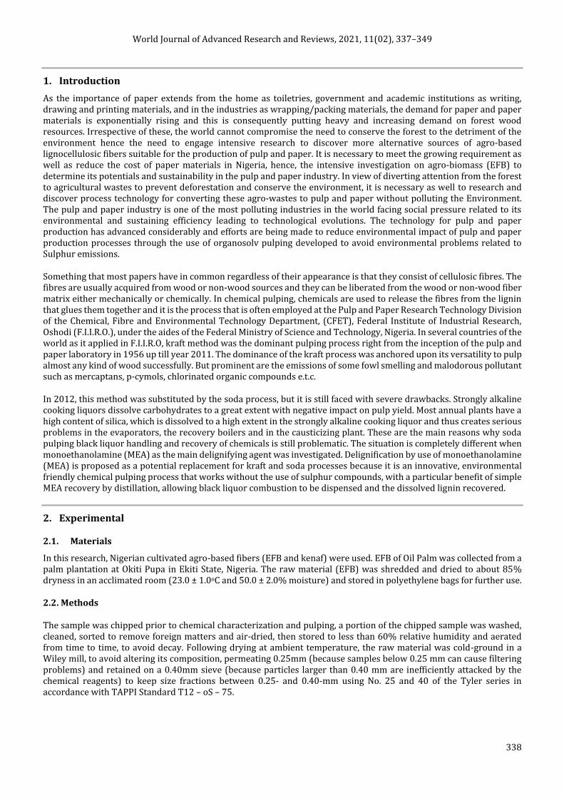
Figure 1 Steps in EFB (Agro-biomass) fractionation and conversion to paper

The feasibility of the application of MEA Process in the Delignification of agro-biomass (EFB) for the Production of Pulp and Paper was evaluated. Central Composite Experimental Design for the pulping conditions furnished the following factors and levels:

• Factor 1: Concentration of cooking liquor: 50%, 75% and 100%MEA • Factor 2: Cooking Time: 60minutes, 90minutes and 120minutes and • Factor 3: Liquor/biomass ratio: 4/1, 6/1 and 8/1

The cooking temperature was maintained at 123±5oC. The conditions of pulping operation were varied as shown in Table 3. The experimental design had 3×3×3 treatments furnishing 27 experimental conditions. Response Surface Design was hence evaluated with respect to a polynomial order to establish a polynomial model. The quadratic terms of the model were hence subjected to various statistical analyses. The behaviour of the cooking process is explained by the following empirical second order polynomial model (Equation 1).

Y% = Ao + A1X1 + A2X2 +A3X3 + A12X1X2 + A13X1X3 + A23X2X3 + A11X12 + A22X22 + A33 X32 …… (1)

Here Y is the Pulp Screened Yield in % and it is calculated as follows: Y% = A- B - R …………..…1a

A

Where A = %Weight of Biomass (before pulping), B= %Weight of Biomass (after pulping) and R= %Weight of Reject. Here Ao is the interception coefficient, A11, A22 and A33 are the quadratic terms, A12, A13 and A23 are the interaction coefficients, and X1, X2, and X3 are the independent variables studied (Cooking time, Liquor charge and Liquor/Biomass Ratio respectively).

In this study, the effect of the three factors (independent variables i.e. X1, X2, and X3) on Pulp Screened Yield from the Monoethanolamine pulping process which in actual terms are Cooking time, Liquor charge and Liquor/Biomass Ratio were investigated at constant maximum temperature value of 123±5oC.

3. Results and discussion

Response Surface Methodology (RSM) is a combination of statistical and mathematical methods used to select the best experimental conditions requiring the lowest number of experiments in order to get appropriate results.

ING

Pulverized EFB (size fraction

between 0.25 and 0.40mm)

g


341

Table 3 Design Layout of Independent Variables (Factors) and the Dependent Variables (Responses) for the Pulping Process

Pulping Scenarios

MEA Conc. (%)

Cooking Time (minutes)

Liquor/Biomass ratio

Total Yield (%)

Screened Yield (%)

Reject (%)

1 50 60 4 44.77 37.76 7.01

2 75 90 4 49.9 49.18 0.72

3 100 120 4 48.12 39.01 9.11

4 50 60 6 43.98 36.67 7.31

5 75 90 6 49.26 48.03 1.23

6 100 120 6 52.03 43.12 8.91

7 50 60 8 42.71 35.12 7.59

8 75 90 8 47.86 46.11 1.75

9 100 120 8 52.01 44.92 7.99

10 50 90 4 50.23 45.77 4.46

11 75 60 4 48.44 43.89 4.55

12 100 60 4 50.96 46.75 4.21

13 50 90 6 48.99 44.32 4.67

14 75 60 6 47.21 42.45 4.76

15 100 60 8 49.79 45.32 4.47

16 50 90 8 48.00 43.12 4.88

17 75 60 8 46.44 41.55 4.89

18 100 60 6 50.32 45.99 4.33

19 50 120 4 52.66 44.77 7.89

20 75 120 4 48.10 44.11 3.99

21 100 90 4 50.21 47.87 2.34

22 50 120 6 51.16 43.19 7.97

23 75 120 6 46.26 43.27 2.99

24 100 90 6 48.67 46.46 2.21

25 50 120 8 49.23 41.22 8.01

26 75 120 8 45.11 42.44 2.67

27 100 90 8 48.09 46.11 1.98

3.1. Statistical Interpretation of Data

Standard errors of the quadratic terms are similar to each other indicating a balanced design. The standard errors are also low which also indicate appropriateness of the result because the lower the error margins the better. VIF stands for Variance Inflation Factor. During regression analysis, VIF assesses whether factors are correlated to each other, which could affect p-values and the model isn't going to be as reliable. The ideal VIF value is 1.0. VIFs above 100 are cause for alarm, indicating coefficients are poorly estimated due to multicollinearity. The numerical value for VIF tells (in decimal form) what percentage the variance (i.e. the standard error squared) is inflated for each coefficient. A rule of thumb for interpreting the variance inflation factor: 1 = not correlated. Between 1 and 5 = moderately correlated. The VIFs of the statistical analyses of the research data generated in this research study range between 1 and 2.58, i.e. below 3. These numerical values indicate that independent factors are moderately correlated. Same goes for the Rᵢ² with a


342

maximum value of 0.6126 which is still within tolerance limit, but not clear yet if it can be used to develop a reliable model since the Rᵢ² is above 0.6.

Table 4 Evaluation of the Experimental Result Layout

Power at 5 % alpha level for effect of Term

Model Terms StdErr** VIF Ri-Squared 1/2 Std. Dev 1 Std. Dev. 2 Std.Dev.

A 0.35 1.32 0.2396 10.0 % 25.7 % 73.9 %

B 0.39 1.70 0.4128 8.9 % 21.0 % 62.9 %

C 0.36 1.70 0.4122 9.6 % 23.9 % 70.1 %

A2 0.48 1.14 0.1232 15.7 % 46.9 % 96.3 %

B2 0.58 1.66 0.3976 12.3 % 34.6 % 87.4 %

C2 0.55 1.38 0.2739 13.1 % 37.6 % 90.5 %

AB 0.57 1.59 0.3712 6.9 % 12.6 % 35.8 %

AC 0.45 1.41 0.2897 8.0 % 17.2 % 51.9 %

BC 0.67 2.58 0.6126 6.3 % 10.4 % 27.2 %

**Basis Std. Dev. = 1.0

Table 5 Sequential Model Sum of Squares

Source Sum of Squares DF Mean Square F Value Prob > F

Mean 40928.63 1 40928.63

Linear 14.25 3 4.75 1.48 0.2569

2FI 0.43 3 0.14 0.037 0.9900

Quadratic 40.56 3 13.52 13.20 0.0008 Suggested

Cubic 9.73 7 1.39 8.16 0.0562 Aliased

Residua 0.51 3 0.17

Total 40994.11 20 2049.71

In statistics, the degrees of freedom (DF) indicate the number of independent values that can vary in an analysis without breaking any constraints. Values of “Prob>F” (P-values) less than 0.0500 indicate model terms are significant. In this case B, C, AB, A² are significant model terms.

Table 6 Model Summary Statistics

Source Std. Dev. R-Squared

Adjusted R-Squared Predicted R-Squared PRESS

Linear 1.79 0.2175 0.0708 -0.1125 72.85

2FI 1.98 0.2242 -0.1339 -0.4249 93.31

Quadratic 1.01 0.8436 0.7029 0.3978 39.44 Suggested

Cubic 0.41 0.9922 0.9506 0.5002 32.73 Aliased


343

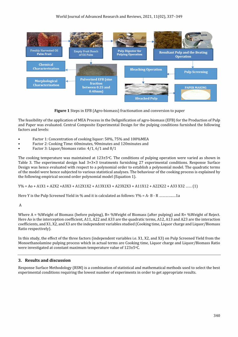
Table 7 Fit Statistics

Std. Dev 1.01 R-Squared 0.8436

Mean 45.24 Adj R-Squared 0.7029

C.V. 2.24 Pred R-Squared 0.3978

PRESS 39.44 Adeq Precision 7.171

A ratio of "Adeq Precision" greater than 4 is desirable. As shown in the Fit Statistics in Table 6, the ratio of 7.171 indicates an adequate signal that this model can be used to navigate the design space. The selected model have insignificant lack-of-fit ensuring that the model fit appropriately with the data generated. The "Adjusted R-Squared" and the "Predicted R-Squared" are too minimal. The Predicted R² of 0.3978 is not as close to the Adjusted R² of 0.7029 as one might normally expect; i.e. the difference is more than 0.2. R2 value of 0.8436 is the percentage of the dependent variable variation explained by the linear model. It indicates slight variation of pulp yield data around it mean as explained by the linear quadratic model. In Table 7, the results of the analysis of variance (ANOVA) are summarized to test the soundness of the model. Analysis of variance (ANOVA) is a statistical technique that subdivides the total variation in a set of data into component parts associated with specific sources of variation for the purpose of testing hypotheses on the parameters of the model. The mean squares values were calculated by dividing the sum of the squares of each variation source by their degrees of freedom, and a 95% confidence level (= 0.05) was used to determine the statistical significance in all analyses.

Table 8 ANOVA for Response Surface Quadratic Model (P < 0.05 is considered as significant)

Source Sum of Squares

Degree of Freedom

Mean Squares

F Value P-Value Remark

Model 55.24 9 6.14 5.99 0.0049 Significant

A-Cooking Time 2.35 1 2.35 2.30 0.1607 Significant

B-Liquor Concentration

22.52 1 22.52 22.0 0.0009 Significant

C-Liquor/Biomass Ratio

6.51 1 6.51 6.35 0.0303 Significant

AB 9.88 1 9.88 9.65 0.0111 Significant

AC 2.03 1 2.03 1.99 0.1891 Significant

BC 2.46 1 2.46 2.41 0.1519 -

A2 36.81 1 36.81 35.95 0.0001 -

B2 3.01 1 3.01 2.94 0.1172 Significant

C2 0.6318 1 0.6318 0.6170 0.4504 Significant

Residual 10.24 10 1.02 -

Lack of Fit 8 Not Significant

Pure error 2 -

Cor Total 65.48 19 -

- R2 = 0.8436 R2adj =0.7029 -

Results were assessed with various descriptive statistics such as the p-value, F-value, and the degree of freedom. As shown in Table 7, a small probability value (p < 0.001) indicates that the model was highly significant and could be used to predict the response function accurately. The Model F-value of 5.99 implies the model is significant. Goodness-of-fit for the model was also evaluated by coefficients of determination R2 (correlation coefficient) and adjusted coefficients


344

of determination R. The large value of the correlation coefficient R2 = 0.8436 indicated a high reliability of the model in predicting pulp screened yield, by which 98.6% of the response variability can be explained by the model.

3.2. Final Equation in Terms of Coded Factors

Pulp Screened Yield =+46.69+1.61*A+0.64*B-0.83*C-0.92*A2-3.24*B2+0.38*C2 1.85*A*B+0.65*A*C+0.74*B*C

The equation in terms of coded factors can be used to make predictions about the response for given levels of each factor. By default, the high levels of the factors are coded as +1 and the low levels are coded as -1. The coded equation is useful for identifying the relative impact of the factors by comparing the factor coefficients.

Final Equation in Terms of Actual Factors: Pulp Screened Yield =

+4.15868

+0.42991 * Liquor Concentration

+0.78101 * Cooking Time

-3.62483 * Liquor/Biomass Ratio

-1.47046E-003 * Liquor Concentration2

-3.59943E-003 * Cooking Time2

+0.094883 * Liquor/Biomass Ratio2

-2.47146E-003 * Liquor Concentration * Cooking Time

+0.012935 * Liquor Concentration * Liquor/Biomass Ratio

+0.012256 * Cooking Time * Liquor/Biomass Ratio

This equation should not be used to determine the relative impact of each factor because the coefficients are scaled to accommodate the units of each factor and the intercept is not at the center of the design space. The equation in terms of actual factors can be used to make predictions about the response for given levels of each factor. Here, the levels should be specified in the original units for each factor. Table 7 is summarized in Table 8 as shown below. The design expert software was used to calculate the coefficients of the second-order fitting equation and the model suitability was tested using the ANOVA test. Therefore, the second-order polynomial equation is expressed as follow:

Pulp Screened Yield = +46.69 + 1.61A + 0.6387B - 0.8261C - 1.85AB + 0.6468AC + 0.7354BC -0.9190A² - 3.23949B² + 0.3795C²…………………2

According to the monomial coefficient value of regression model Equation (2), X1 = A = 1.6129 (Cooking Time), X2 = B = 0.6387 (Liquor Concentration) and X3 = C = -0.826071 (Liquor/Biomass Ratio), and the order of priority among the main effect of impact factors is Cooking Time (X1) > Liquor Concentration (X2) > Liquor/Biomass Ratio (X3).

Table 9 Coefficient Table for the Quadratic Model

Intercept A B C AB AC BC A2 B2 C2

Pulp Screened Yield

46.6897 1.6129 0.6387 -0.826071 -1.8536 0.646764 0.735365 -0.919037 -3.23949 0.379532

p-values 0.1607 0.0009 0.0303 0.0111 0.1891 0.1519 0.0001 0.1172 0.4504

p-value shading: p<0.05 0.05≤p<0.1 p≥0.1

The "Model F-value" of 5.99 implies the model is significant which was confirmed by Values of "Prob > F" (p-value) less than 0.0500 indicating that the model terms are significant in surface response analysis. In this case A, B, AC and BC are


345

significant model terms. The positive "Pred R-Squared" value above (0.3978) implies that the current model is a better predictor of the response than the overall mean.

3.3. Diagnostics of the Linear Regression (Quadratic) Model

In statistics, the actual value is the value that is obtained by observation or by measuring the available data. It is also called the observed value. The predicted value is the value of the variable predicted based on the regression analysis. The difference between the actual value or observed value and the predicted value is called the residual in regression analysis. Each actual value has a predicted value and hence each data point has one residual. However, to evaluate this quadratic the model, we regress predicted vs. actual (observed) values or vice versa and compare slope and intercept parameters against 1:1 line.

Figure 3 Plot of Predicted vs Actual Values Figure 4 Normal Plot of Residual vs Predicted Values

The residuals are represented graphically by means of a residual plot as shown in figure 4. This normal probability plot indicates whether the residuals follow a normal distribution, thus follow the straight line. Here, the scatter had a definite pattern along the straight line which indicates that a transformation of the response may provide a better analysis.

The Residuals vs. Predicted plot is a plot of the residuals versus the ascending predicted response values. It tests the assumption of constant variance. The plot should be a random scatter (constant range of residuals across the graph). In Figure 5, the residual plots are randomly scattered (spread) around the horizontal axis, indicating the appropriateness of the linear regression (quadratic) model.

Figure 5 Plot of Residual vs Predicted Values Figure 6 Effect of Interactions of the three factors

Figure 6 describes the interaction of the three (3) factors in relation to pulp screened yield. The graph of interaction of the three factors reveal that as the pulping temperature and cooking time increased, pulp screened yield correspondingly increased up to a certain point and decreased. The green, red and black points on the interaction graph clearly indicated the points of deviation. Reading from the graph confirm that beyond 90 minutes cooking time, 20% Soda concentration and 150oC cooking temperature, there was irrecoverable deviation from the trend of increase in pulp screened yield. It is clear from the graph that the main interacting factors are cooking time and liquor concentration.

Design-Expert® Software

Trial Version

Pulp Screened Yield

Color points by value of

Pulp Screened Yield:

42.45 49.18

X: Actual

Y: Predicted

Predicted vs. Actual

42

44

46

48

50

42 44 46 48 50


346

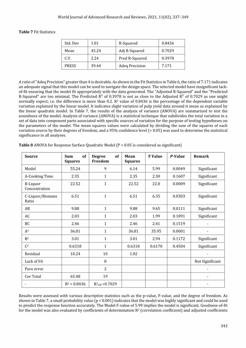
3.4. Effects of Model Parameters and Their Interactions

Figure 7 Perturbation vs Pulp Screened Yield Figure 8 Effect of Interaction of Model Parameters on Pulp Screened Yield

The significance of each model parameter was determined by means of Fischer’s F-value and p-value. The F-value is the test for comparing the curvature variance with residual variance and probability >F (p-value) is the probability of seeing the observed F-value if the null hypothesis is true. Small probability values call for rejection of the null hypothesis and the curvature is not significant. Therefore, the larger the value of F and the smaller the value of p, the more significant the corresponding coefficient is. As shown in Table 7, we concluded that the independent variables of the quadratic model, including the cooking time (X1), liquor concentration (X2) and the interactions between the cooking time (X1) and Liquor concentration (X2) are highly significant parameters because p < 0.001. The p value >0.05 means that the model terms are insignificant. We can see from Table 7 that interactions between the cooking time and liquor/biomass ratio and the interaction between liquor concentration and liquor/biomass ratio are significant.

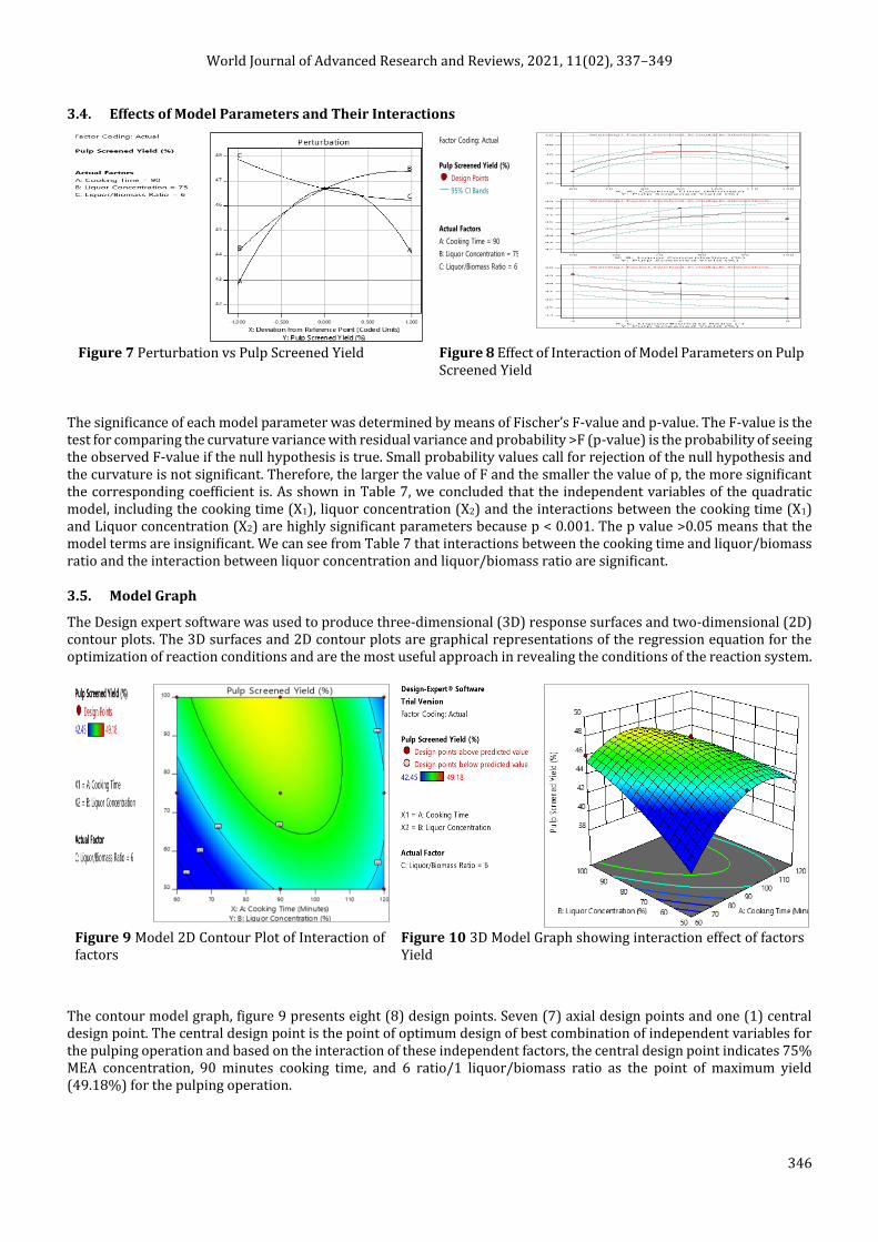
3.5. Model Graph

The Design expert software was used to produce three-dimensional (3D) response surfaces and two-dimensional (2D) contour plots. The 3D surfaces and 2D contour plots are graphical representations of the regression equation for the optimization of reaction conditions and are the most useful approach in revealing the conditions of the reaction system.

Figure 9 Model 2D Contour Plot of Interaction of factors

Figure 10 3D Model Graph showing interaction effect of factors Yield

The contour model graph, figure 9 presents eight (8) design points. Seven (7) axial design points and one (1) central design point. The central design point is the point of optimum design of best combination of independent variables for the pulping operation and based on the interaction of these independent factors, the central design point indicates 75% MEA concentration, 90 minutes cooking time, and 6 ratio/1 liquor/biomass ratio as the point of maximum yield (49.18%) for the pulping operation.


Trial Version

Factor Coding: Actual

Pulp Screened Yield (%)

Design Points

95% CI Bands

Actual Factors

A: Cooking Time = 90

B: Liquor Concentration = 75

C: Liquor/Biomass Ratio = 6

X: A : Cooking Time (Minutes)

60 70 80 90 100 110 120

Y: Pulp Screened Yield (%)

40

42

44

46

48

50 Warning! Factor involved in multiple interactions.

X: B: Liquor Concentration (%)

50 60 70 80 90 100


42

43

44

45

46

47

48


X: C: Liquor/Biomass Ratio (-)

4 5 6 7 8


44

45

46

47

48

49



Trial Version


Pulp Screened Yield (%)

Design Points

95% CI Bands

Actual Factors

A: Cooking Time = 90

B: Liquor Concentration = 75

C: Liquor/Biomass Ratio = 6

X: A : Cooking Time (Minutes)

60 70 80 90 100 110 120


40

42

44

46

48


X: B: Liquor Concentration (%)

50 60 70 80 90 100


42

43

44

45

46

47

48


X: C: Liquor/Biomass Ratio (-)

4 5 6 7 8


44

45

46

47

48

49



347

Curve fitting, also known as regression analysis, is used to find the "best fit" line or curve for a series of data points. There are five (5) design points around the 3D surface model graph described by Figure 10 which presents two (2) sets of design points. One (1) design point above the curve fitting indication point of maximum yield and four (4) design point at the edge of the curve fitting below the point of maximum yield. The curve fitting on the 3D surface model graph examined the relationship between three predictors (independent variables i.e. MEA concentration, cooking time and liquor/biomass ratio) and a response variable (dependent variable i.e. pulp screened yield), with the goal of defining a "best fit" model of the relationship. The red dotted lines are lines indicating on each factor the points of maximum yield. These are the design points of the optimum parameters of the independent variables furnishing the best pulping conditions at 90minutes cooking time, 75% MEA concentration and 4/1 liquor/biomass ratio. For further confirmation of this, we move on to conduct optimization analysis.

3.6. Optimization Analysis

Numerical optimization uses the models to search the factor space for the best trade-offs to achieve multiple goals, while Graphical optimization uses the models to show the volume where acceptable response outcomes can be found. In order to select the optimum parameters for the pulping conditions maximizing pulp yield and minimizing all possible constraints, design expert presented a range of solution choices which were compared to determine which might be “best” in terms of considering all possible advantage/benefit (minimal cost, maximal profit, minimal error and optimal design) with the goal of understanding and resolving the modelling issue (ensuring the model fit and the data fit perfectly). In order to specify the best cooking conditions so as to maximize the potentials of the monoethanolamine pulping process, the data generated from the pulping operations were subjected to optimization analysis using Design Expert Software 12 and results are presented in Table 9.

Individual desirability: The closer the predicted responses are to the target requirements, the closer the desirability will be to 1.

Composite desirability: The composite desirability combines the individual desirabilities into an overall value, and reflects the relative importance of the responses. The higher the desirability the closer it will be to 1. Desirability is measured on a 0 to 1 scale. Figure 12 shows that the combination of all individual desirability of all the factors and response sum up to 1 (unity) which is an ultimate indication of high desirability. These desirability values indicate how close the predicted responses are to our target requirements.

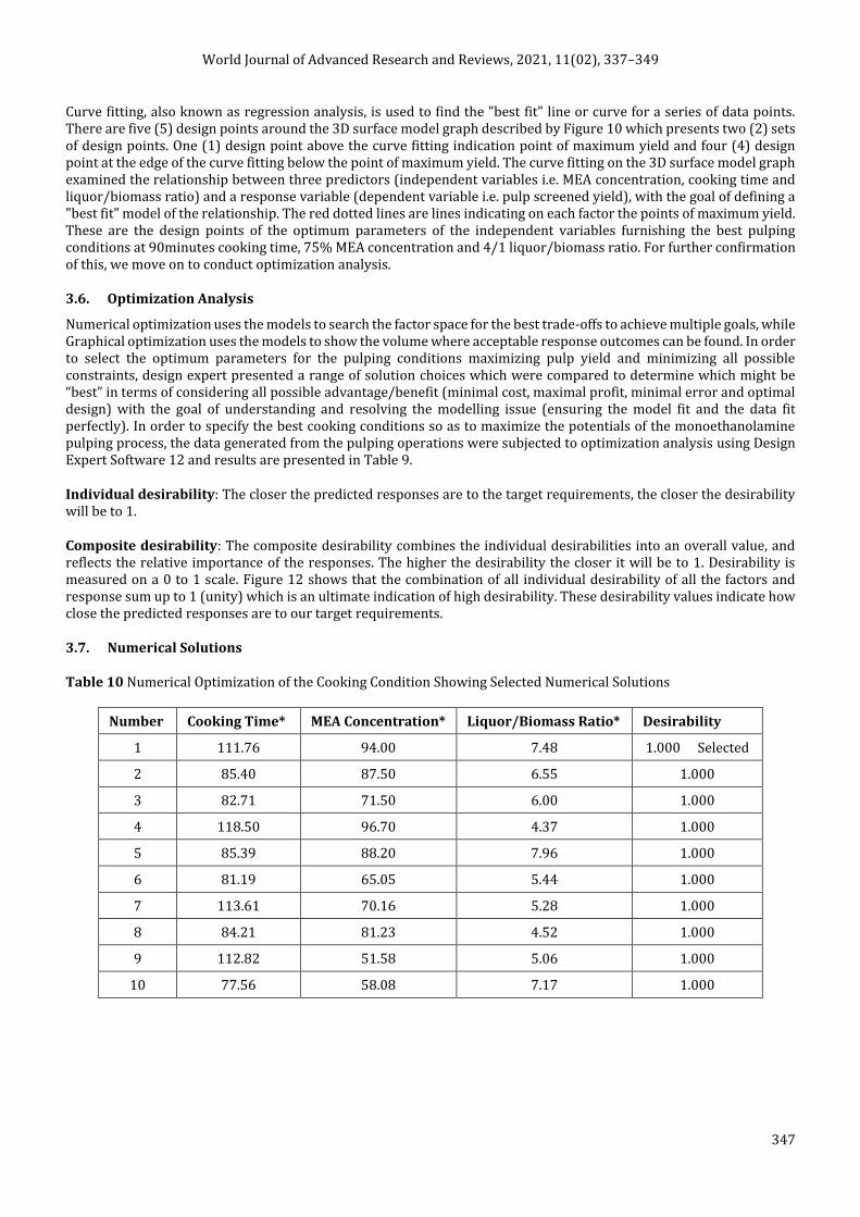
3.7. Numerical Solutions

Table 10 Numerical Optimization of the Cooking Condition Showing Selected Numerical Solutions

Number Cooking Time* MEA Concentration* Liquor/Biomass Ratio* Desirability

1 111.76 94.00 7.48 1.000 Selected

2 85.40 87.50 6.55 1.000

3 82.71 71.50 6.00 1.000

4 118.50 96.70 4.37 1.000

5 85.39 88.20 7.96 1.000

6 81.19 65.05 5.44 1.000

7 113.61 70.16 5.28 1.000

8 84.21 81.23 4.52 1.000

9 112.82 51.58 5.06 1.000

10 77.56 58.08 7.17 1.000


348

Figure 11 Optimization Contour Plot of Numerical Solution

Figure 12 Desirability Plot of Numerical Solution

3.8. Graphical Solutions

Figure 13 2D Optimization Contour Plot Confirming Numerical Solution

Figure 14 Model 2D Overlay Contour Plot of Graphical Optimization Solution

Table 11 Cooking Condition Showing Selected Numerical Solutions

Number Cooking Time Liquor Concentration

Liquor/Biomass Ratio

Pulp Screened Yield

Desirability

1 111.76 94.00 7.48 49.18 1.00 Selected

The plot critical level is the confidence level at which the contour plots of the two data sets meet at a single point. This is the minimum confidence level at which the contour lines of the two different data sets overlap. At any confidence level below this minimum confidence level, the contour lines of the two data sets will not overlap and there will be a statistically significant difference between the two populations at that level.

4. Conclusion and Recommendation

Proceeding experimental results were generated at statistically estimated 95% confidence level, and as can be seen in Figure 14, the overlap contour graph furnished X1= 111.76 for cooking time and X2= 94.00 for MEA-concentration. We can then conclude that there is a statistically significant difference between the data sets at the 95% confidence level. Based on the results obtained, the use of 90 minutes cooking time, 75% MEA concentration and 4/1 liquor biomass ratio led to the best results in terms of screened yield (49.18%) for the overall MEA pulping operations when cooking temperature is maintained at 123±5oC. But further investigation using series of statistical analysis presented selected solution for the optimal cooking condition as follow: 111.76minutes Cooking Time, 94.00% Liquor Concentration, and 7.48 Liquor/Biomass Ratio. The Optimization contour graph confirms these predicted values from the numerical solution. The results show that there is an impact of cooking time, MEA concentration and liquor/biomass ratio over the screened yield and there is also an interaction between cooking time and MEA concentration. The model prediction for maximum screen yield was compared to the experimental result at optimal operating conditions. A good agreement between the model prediction and experimental results confirms the soundness of the developed model.

DESIGN-EXPERT Plot

Overlay PlotDesign Points

X = A: Cooking TimeY = B: MEA Concentration

Actual FactorC: Liquor/Biomass Ratio = 6.00

Overlay Plot

A: Cooking Time

B: ME

A Conc

entrati

on

60.00 75.00 90.00 105.00 120.00

50.00

62.50

75.00

87.50

100.00


Trial Version


All Responses

Design Points

0 1

X1 = A: Cooking Time

X2 = B: Liquor Concentration

Actual Factor

C: Liquor/Biomass Ratio = 4 60 70 80 90 100 110 120

50

60

70

80

90

100Desirability

X: A: Cooking Time (Minutes)

Y: B: Liquor Concentration (%)

0.2

0.2

0.4

0.4

0.6

0.6

Desirability 0.742957

60 70 80 90 100 110 120

50

60

70

80

90

100Pulp Screened Yield (%)

X: A: Cooking Time (Minutes)

Y: B: Liquor Concentration (%)

42

44

44

46

46

48

Prediction 46.4479


349

References

[1] Anonymous. Technical Association of the Pulp and Paper Industry: Sampling and Preparing Wood for analysis (TAPPI Standard Test Method T257 om-02), Atlanta, USA. 2012.

[2] Anonymous. Technical Association of the Pulp and Paper Industry: Moisture in pulp, paper and paperboard (TAPPI Standard Test Method T 412 om-06), Atlanta, USA. 2006.

[3] Anonymous. Technical Association of the Pulp and Paper Industry: Water solubility of wood and pulp (TAPPI Standard Test Method T207 cm-99), Atlanta, USA. 1999.

[4] Anonymous. Technical Association of the Pulp and Paper Industry: Solvent extractives of wood and pulp (TAPPI Standard Test Method T204 cm-97), Atlanta, USA. 2007.

[5] Anonymous. Technical Association of the Pulp and Paper Industry: Acid-insoluble lignin in wood and pulp (TAPPI Standard Test Method T 222 om-02), Atlanta, USA. 2006.

[6] Anonymous. Technical Association of the Pulp and Paper Industry: Alpha-, beta- and gamma-cellulose in pulp (TAPPI Standard Test Method T203 cm-99), Atlanta, USA. 1999.

[7] Anonymous. Technical Association of the Pulp and Paper Industry: One percent sodium hydroxide solubility of wood and pulp (TAPPI Standard Test Method T212 om-02), Atlanta, USA. 2002.

[8] Anonymous. Technical Association of the Pulp and Paper Industry: Ash in wood, pulp, paper and paperboard: combustion at 525°C (TAPPI Standard Test Method T211 om-02), Atlanta, USA. 2002.

MEA-conversion of agro-wastes to paper-pulp: Optimization ...

Documents

Transcript of MEA-conversion of agro-wastes to paper-pulp: Optimization ...