Structural Dynamics

The spring force is given by                        and F(t) is the driving force.  Start by applying Newton’s second law (F=ma).

We will now look at free vibrations.

Considering the free vibration of the mass—that is, when F(t) = 0.

Spring mass system.

Setting m = 0.

We obtain.

Free body diagrams of spring mass system.

The free vibration of the system will take the form of simple harmonic motionbelow.

Time/displacement curve.

The motion defined above is called simple harmonic motion. The displacementand acceleration are proportional but of opposite directions..

xm is the maximum displacement  or amplitude of the vibration.

The period  is the time necessary to make a full cycle.

Time/displacement curve.

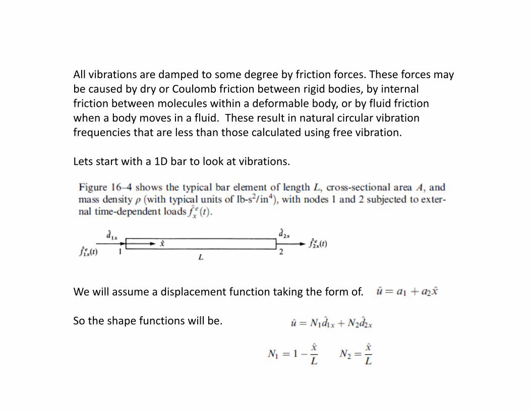
All vibrations are damped to some degree by friction forces. These forces may be caused by dry or Coulomb friction between rigid bodies, by internalfriction between molecules within a deformable body, or by fluid frictionwhen a body moves in a fluid.  These result in natural circular vibration frequencies that are less than those calculated using free vibration.

Lets start with a 1D bar to look at vibrations.

We will assume a displacement function taking the form of.

So the shape functions will be.

The strain/displacement relationship is given by.

1

2

uu

The stress/strain relationship is given by.

D B U

Time dependence:  The bar is not in equilibrium under a time‐dependent forceso f1x f2x.

At each node ‘the external (applied) force  minus the internal force is equal to the nodal mass times acceleration.’

We add this internal force F = ma to each nodal force to obtain.

The masses m1 and m2 are lumped to each of the nodes to obtain.

exf

The external nodal force becomes.

The element stiffness matrix is.

The lumped mass matrix is given by.

The acceleration term is. 

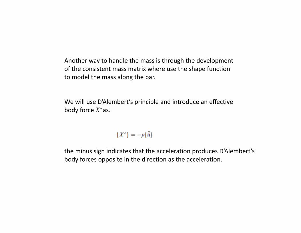
Another way to handle the mass is through the developmentof the consistent mass matrix where use the shape function to model the mass along the bar.

We will use D’Alembert’s principle and introduce an effective body force Xe as.

the minus sign indicates that the acceleration produces D’Alembert’sbody forces opposite in the direction as the acceleration.

We will use                                                    and substitute 

for  {X} gives us.

Using                          and completing the derivatives.

The element mass matrix is given by.

Substituting for interpolation functions:

For a 1D bar one gets:

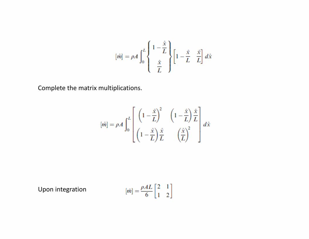
Complete the matrix multiplications.

Upon integration

Assembly

Numerical Integration in Time

Several different methods are available to do the numerical integration.

We will cover central‐difference and the Newmark‐Beta.

The central difference method is based on finite difference expressions in time for velocity and acceleration at time t given by the following:

With a Taylor expansion acceleration can be defined in terms of displacements.

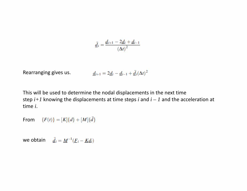
Rearranging gives us.

This will be used to determine the nodal displacements in the next timestep i+1 knowing the displacements at time steps i and i – 1 and the acceleration attime i.

From

we obtain 

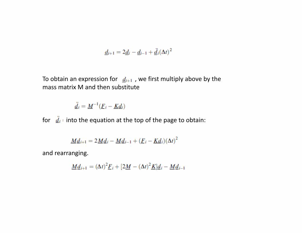
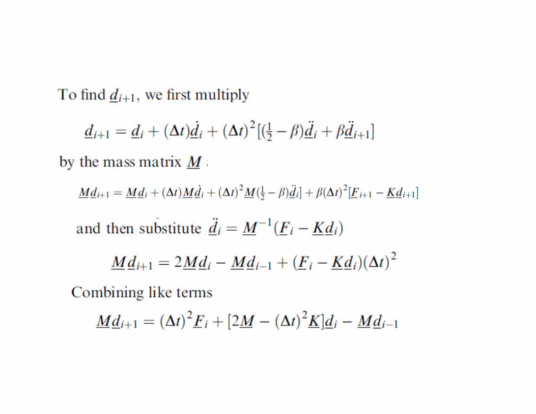
To obtain an expression for  , we first multiply above by the mass matrix M and then substitute 

for          into the equation at the top of the page to obtain:

and rearranging.

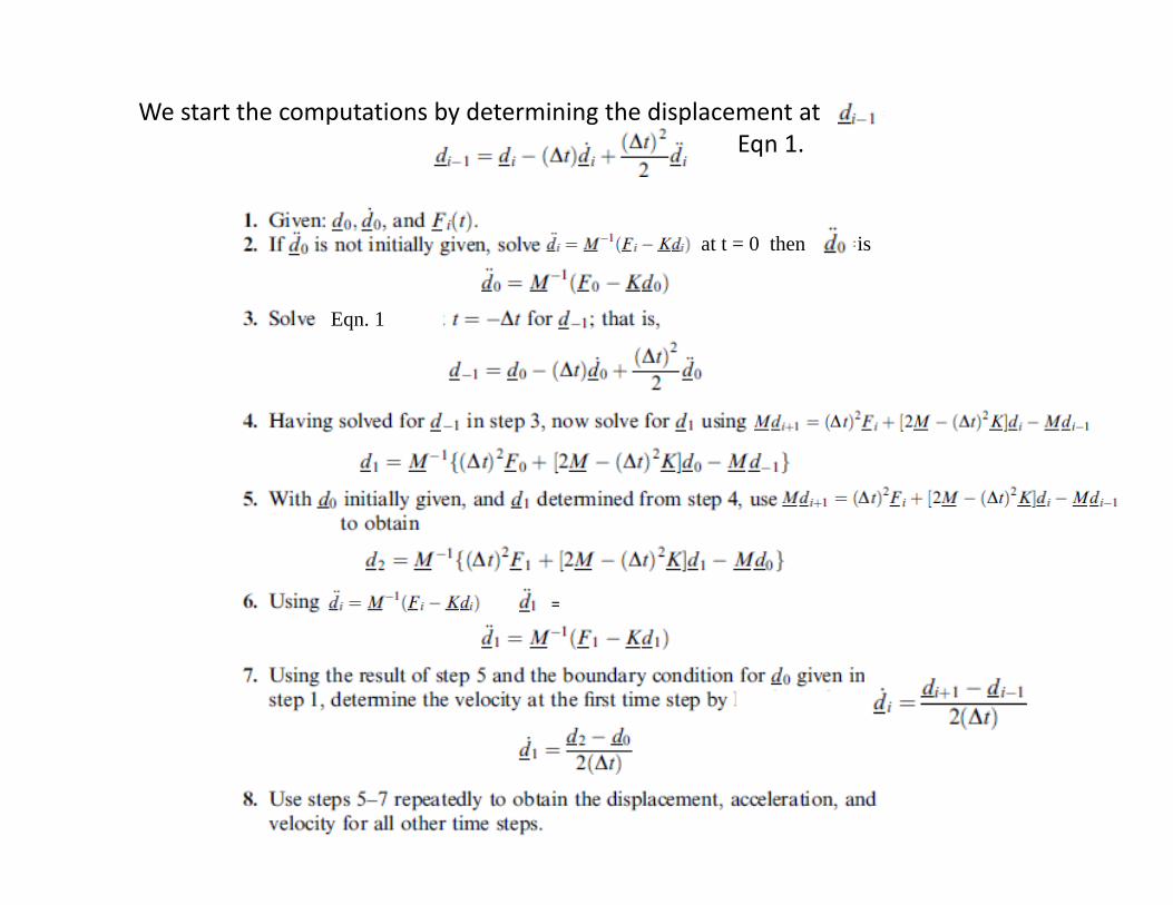
We start the computations by determining the displacement atEqn 1. 

at t = 0 then is

Eqn. 1

==

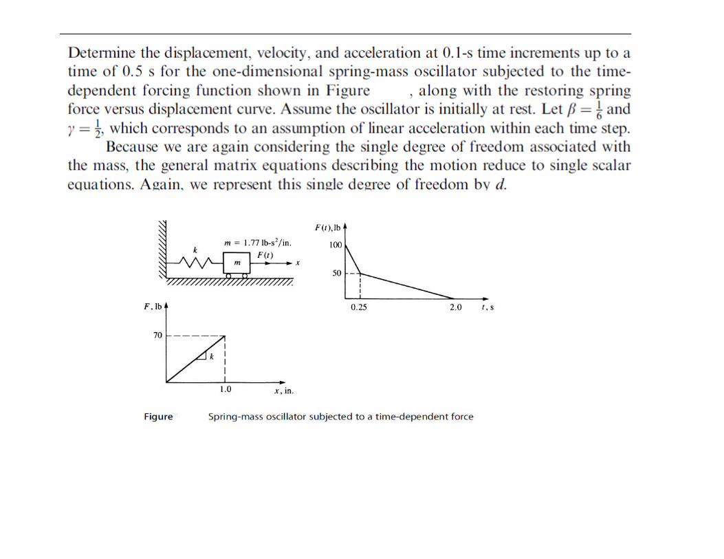
Determine the displacement, velocity, and acceleration at 0.05‐s time intervals up to 0.2 s for the one‐dimensional spring‐mass oscillator subjected to the time‐dependent forcing function shown in the figure below. This forcing function is a typical one assumed for blast loads. The restoring spring force versus displacement curve is also provided. [Note that the bar in the figure represents a one‐element bar with its left endfixed and right node subjected to F(t) when a lumped mass is used.

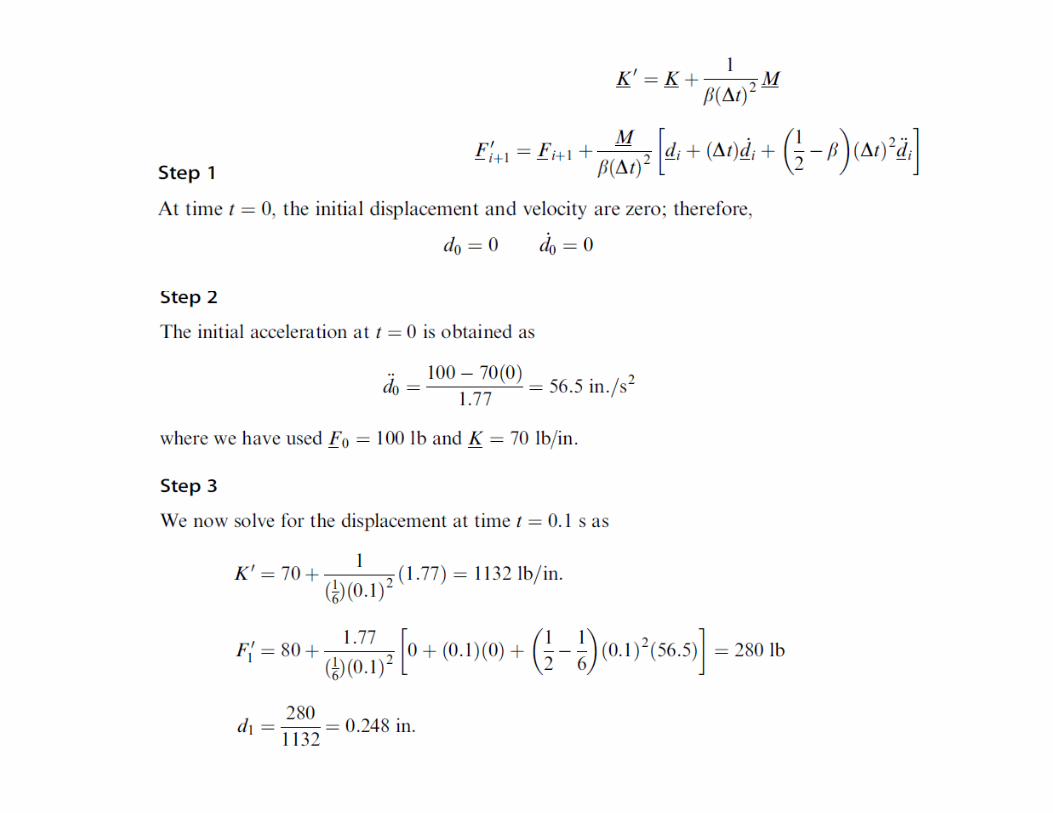
Step 1

At time = 0, the displacement and velocity are

m = 31.83 lb-s/in2

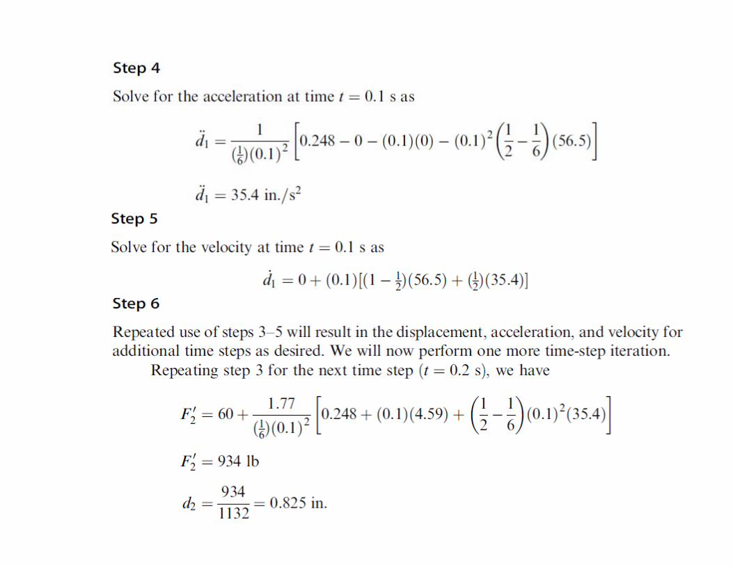
Step 4

Use

Newmark‐Beta Method

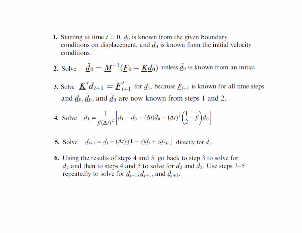
Newmark‐Beta equations

where  and  are parameters chosen by the user. The parameter is generally chosen between 0 and 1/4, and  is often taken to be 1/2.

= 1/2 and  = 1/4 , gives stable analysis  results.

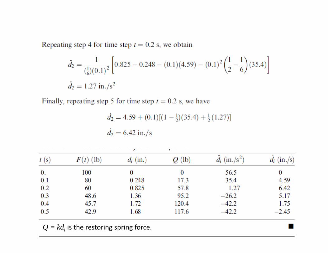
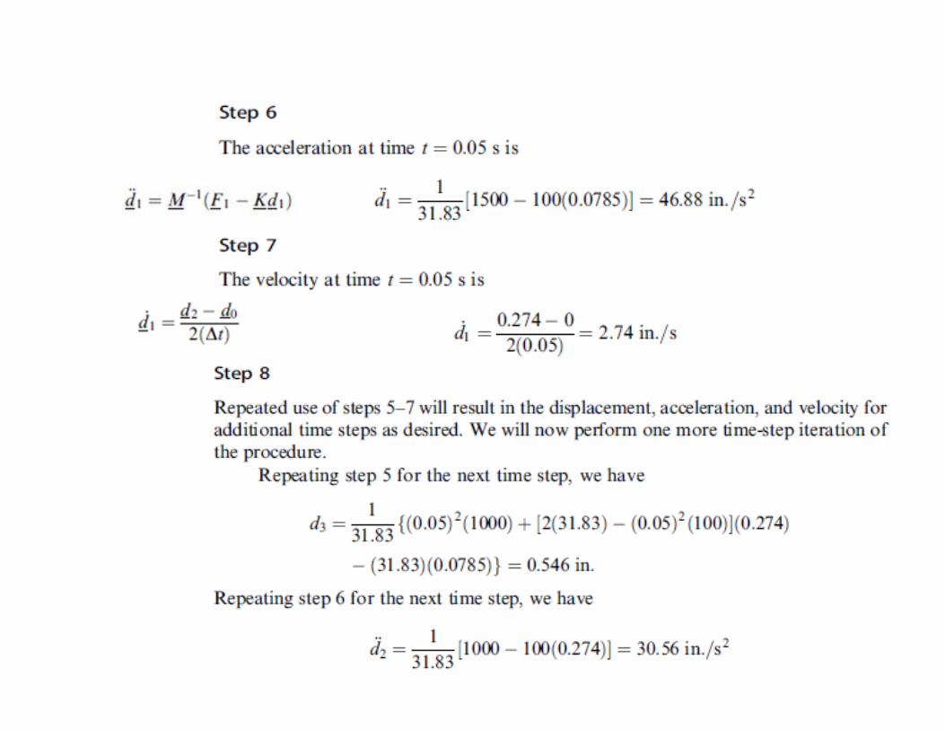
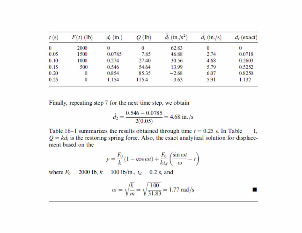
Q = kdi is the restoring spring force.

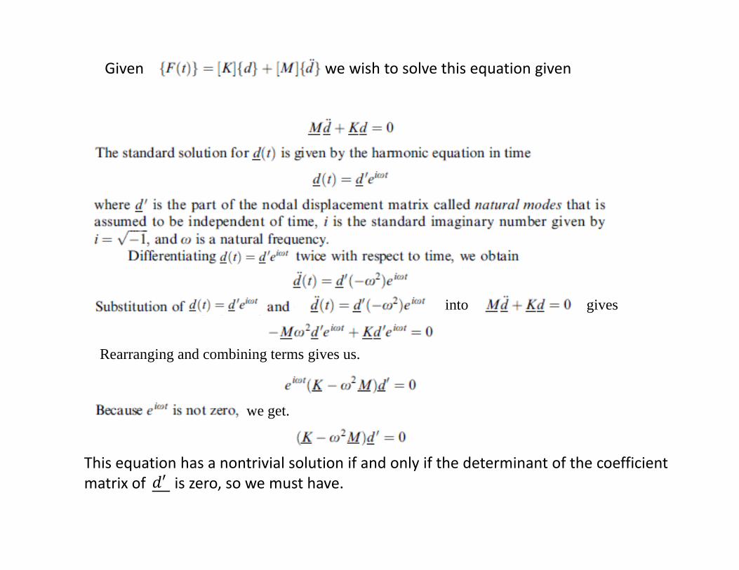
Given                                               we wish to solve this equation given  

into gives

Rearranging and combining terms gives us.

we get.

This equation has a nontrivial solution if and only if the determinant of the coefficient matrix of  is zero, so we must have.′ 

This equation has a nontrivial solution if and only if the determinant of the coefficient matrix of  is zero, so we must solve.′ 

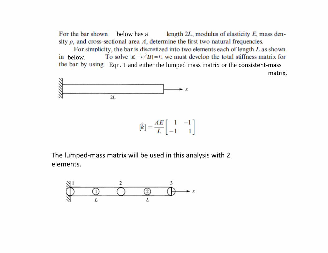
below has a

below. Eqn. 1 and either the lumped mass matrix or the consistent‐mass 

matrix.

The lumped‐mass matrix will be used in this analysis with 2 elements.

Assemble the global stiffness matrix. 

The mass matrices are. 

Assembled

Assemble all the components and apply the boundary conditions(which is the same as:

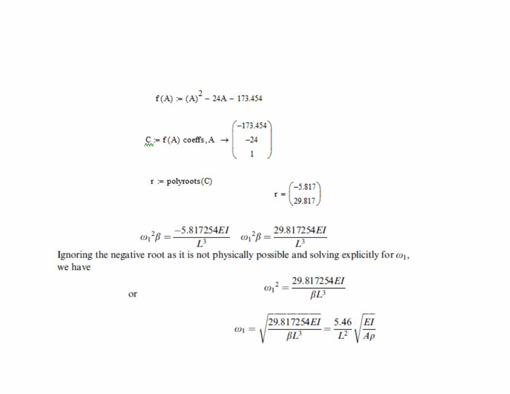
Dividing above by AL and letting  = E/ ( L2), we obtain:

Take the determinant of this

gives.so

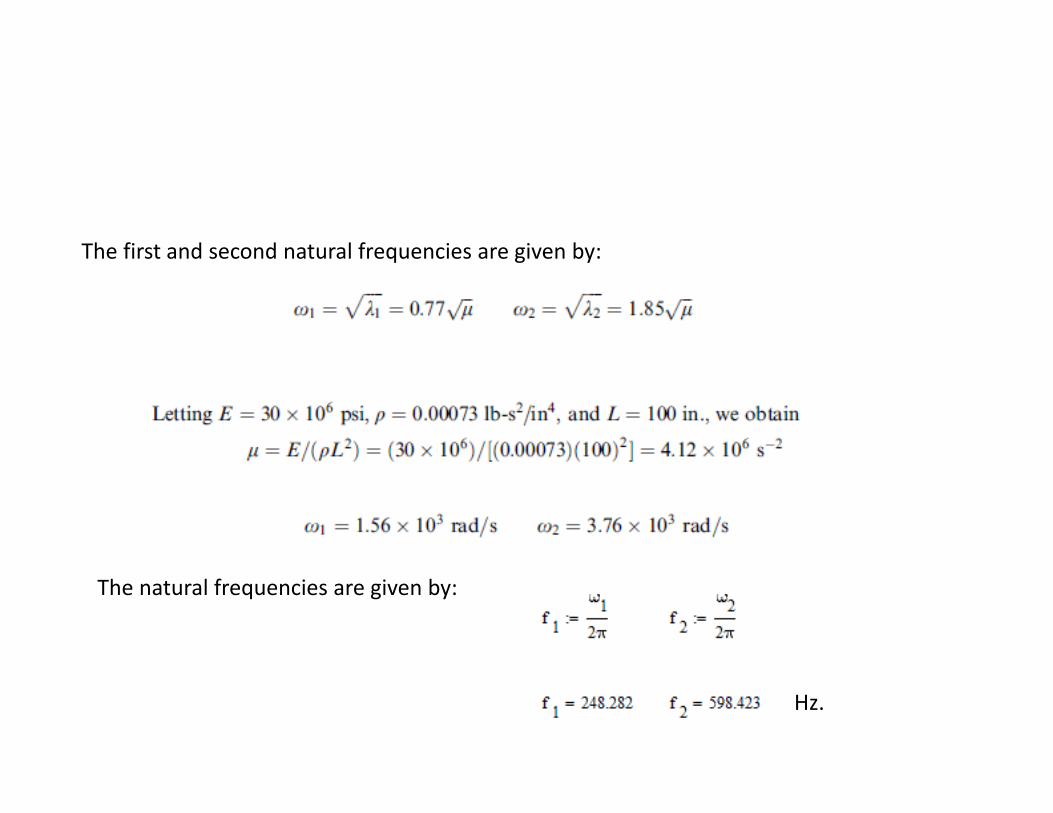
The first and second natural frequencies are given by:

The natural frequencies are given by:

Hz.

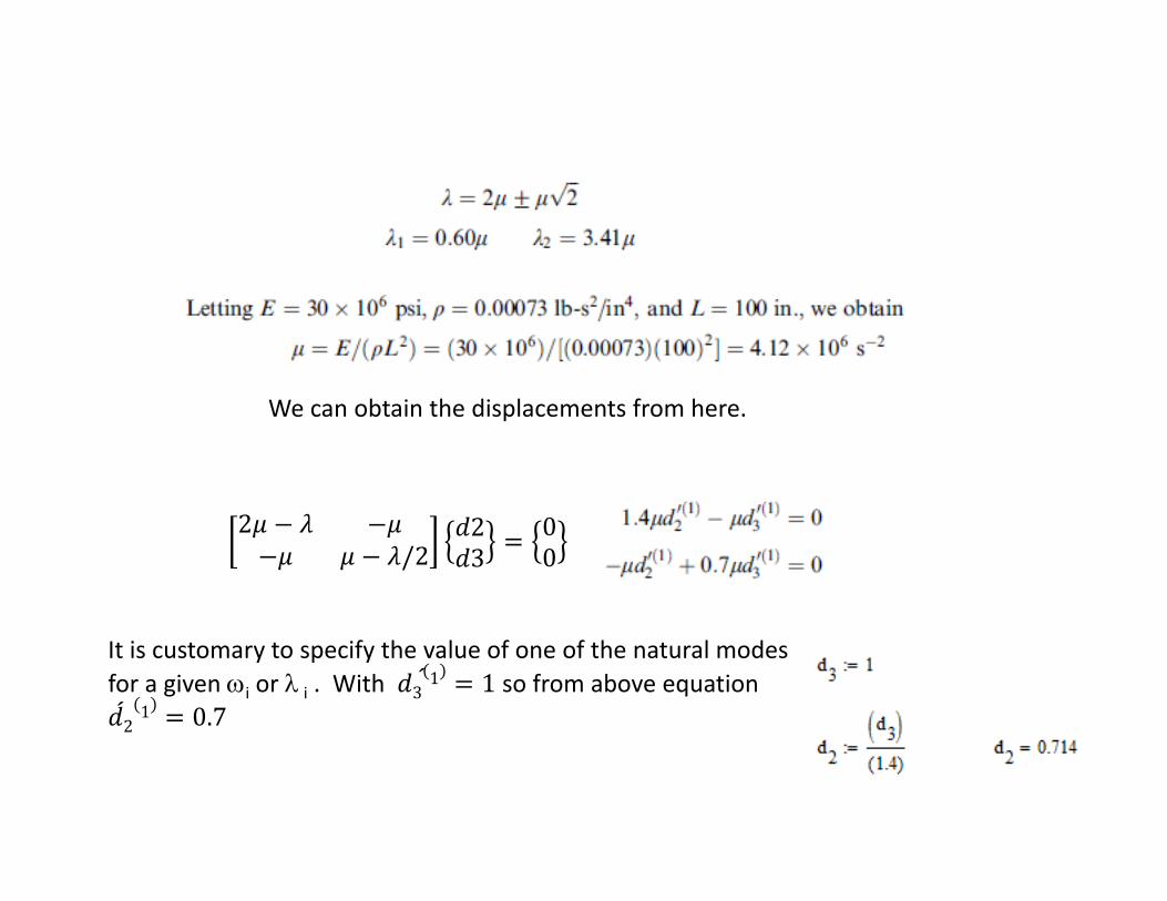
We can obtain the displacements from here.

It is customary to specify the value of one of the natural modes for a given i or  i .  With  3

1 1 so from above equation 21 0.7

2/2

23

00

Substituting  2topequation.

Again assuming  31 1

2/2

23

00

Using the previous results we shall now solve a time dependentproblem using the same problem as the natural frequency workabove.

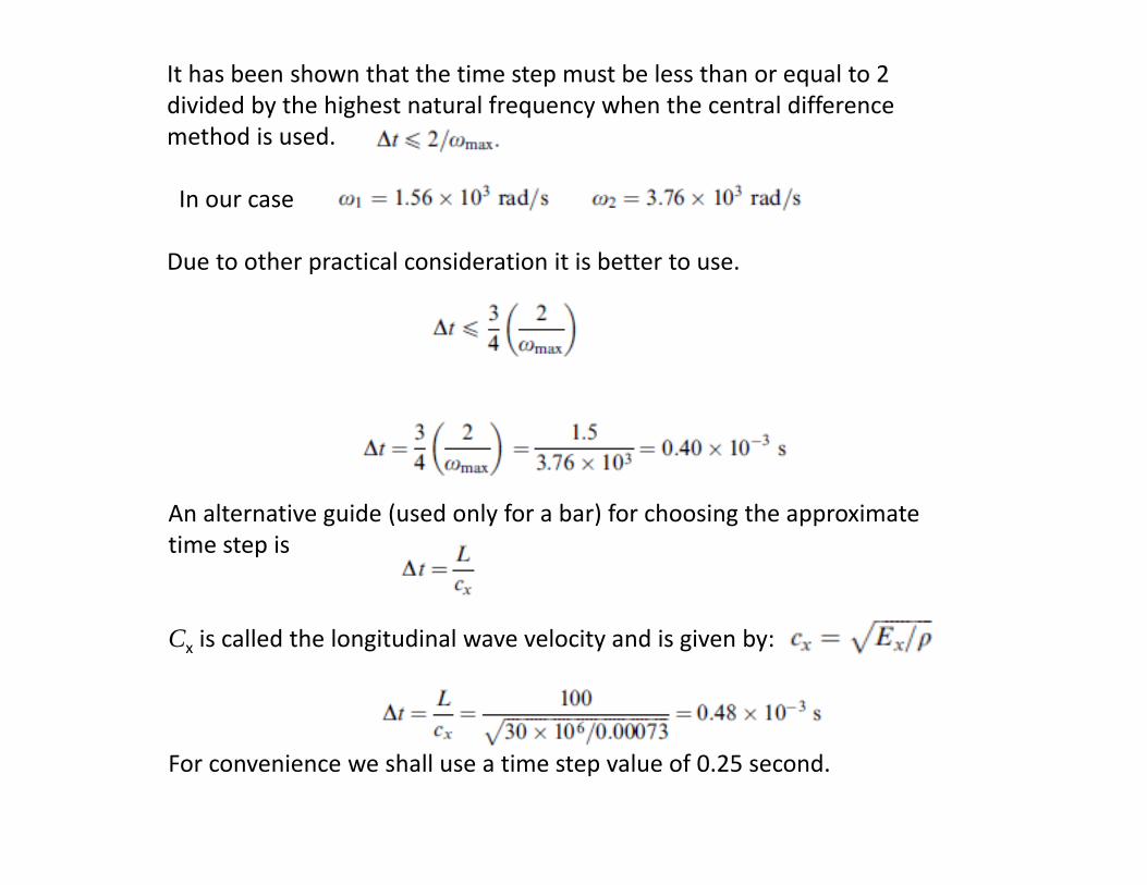
It has been shown that the time step must be less than or equal to 2 divided by the highest natural frequency when the central difference method is used.   

In our case

Due to other practical consideration it is better to use. 

An alternative guide (used only for a bar) for choosing the approximatetime step is

Cx is called the longitudinal wave velocity and is given by:

For convenience we shall use a time step value of 0.25 second. 

Thus eliminating the first row and columns of above and rearranging.

Solve for d1 using.

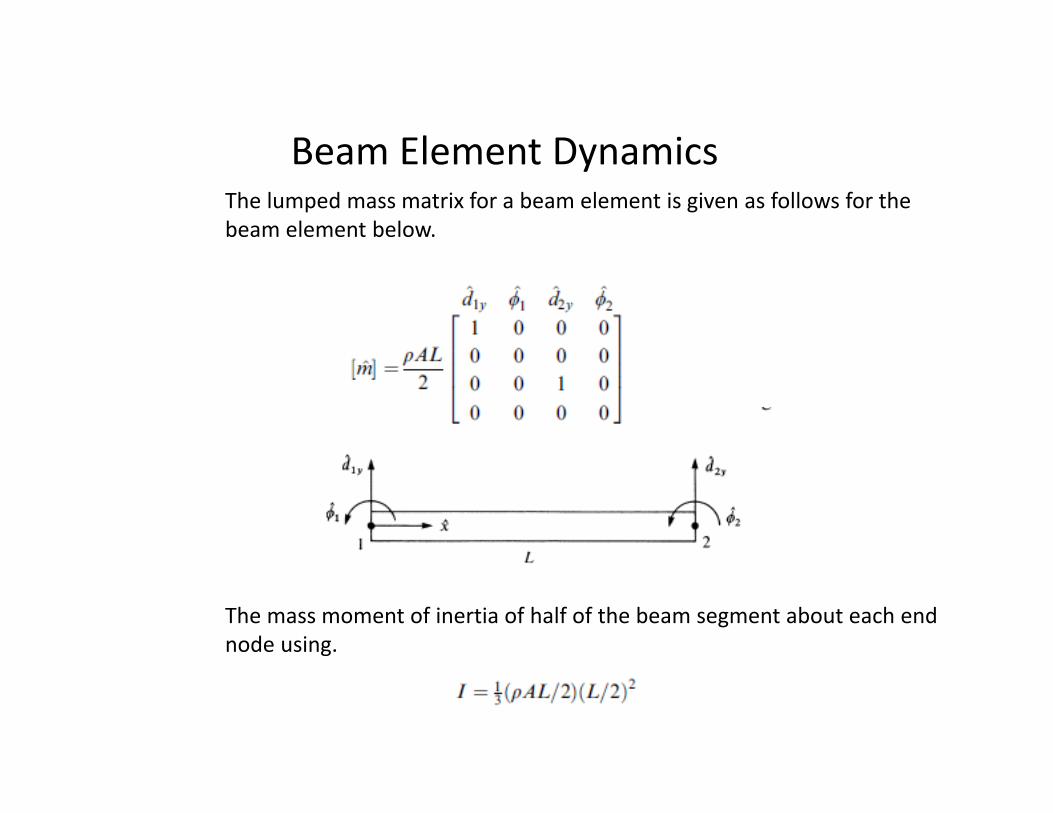
Beam Element DynamicsThe lumped mass matrix for a beam element is given as follows for the beam element below.

The mass moment of inertia of half of the beam segment about each end node using.

The consistent mass matrix is determined by using the shape functions: 

The mass matrix becomes.

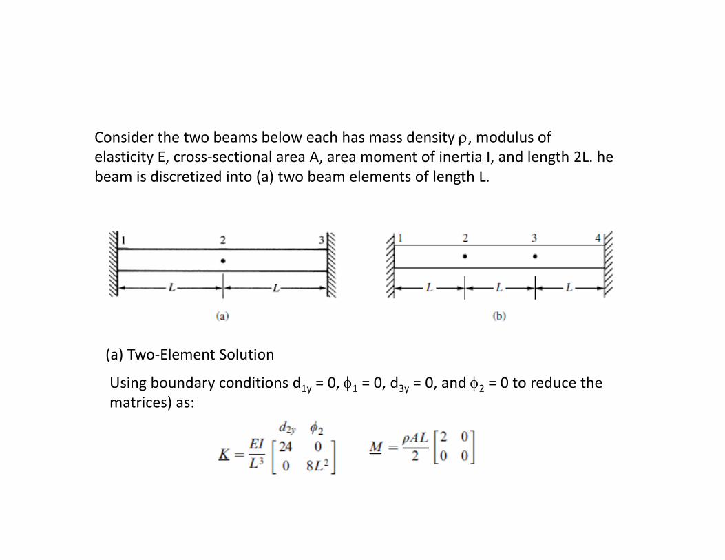
Consider the two beams below each has mass density , modulus ofelasticity E, cross‐sectional area A, area moment of inertia I, and length 2L. he beam is discretized into (a) two beam elements of length L.

(a) Two‐Element Solution

Using boundary conditions d1y = 0, 1 = 0, d3y = 0, and 2 = 0 to reduce the matrices) as:

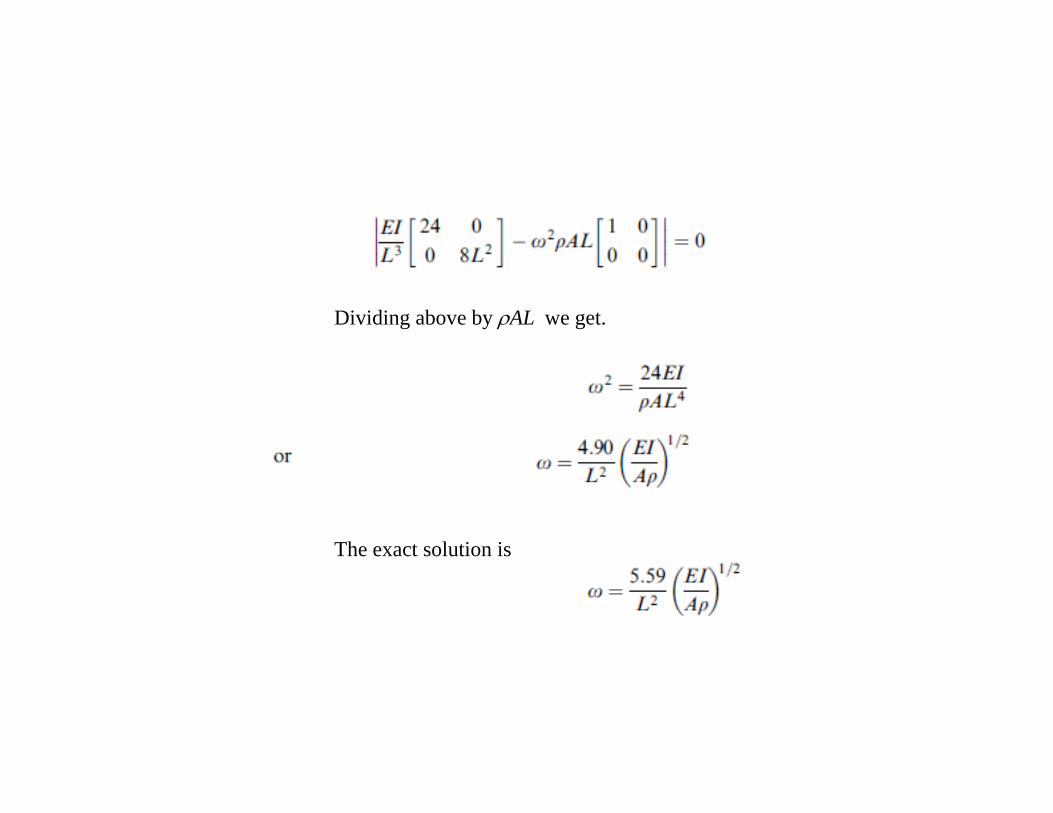
Dividing above by AL we get.

The exact solution is

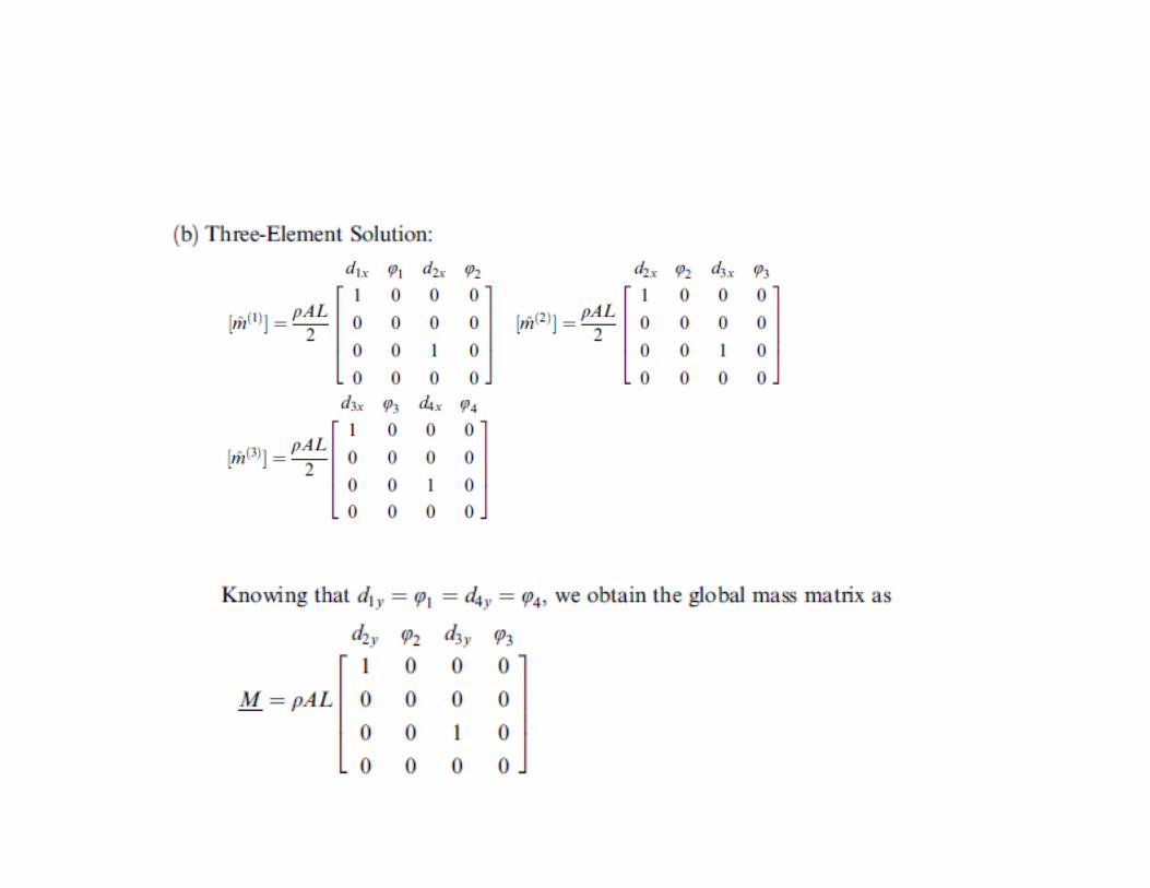
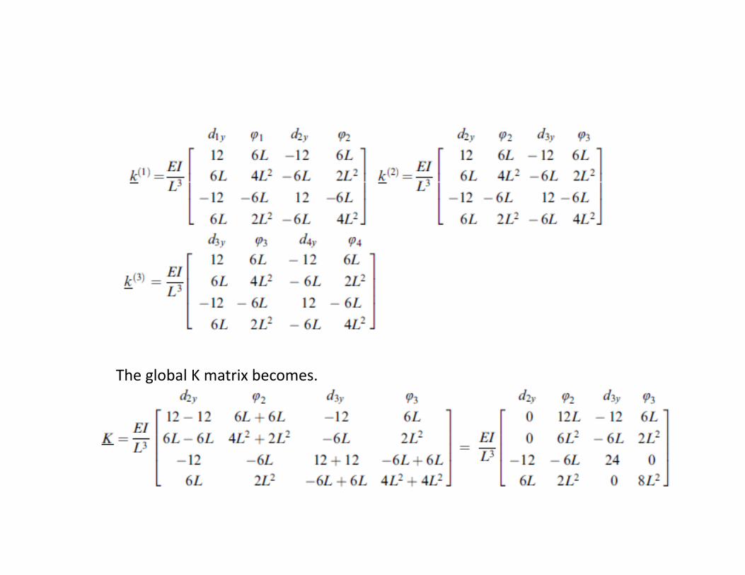
The global K matrix becomes.

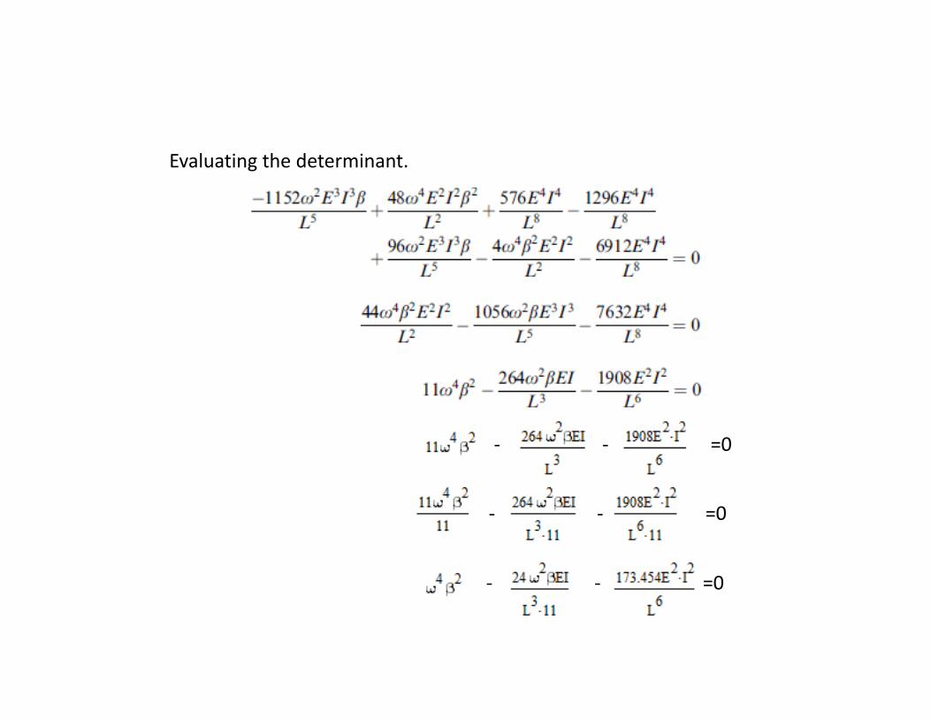
Evaluating the determinant.

‐ ‐ =0

‐ ‐ =0

‐ ‐ =0