I

EXECUTIVE SUMMARY

Background

Due to the perceived occurrence of high-intensity storms more frequently than

expected, the Michigan Department of Transportation (MDOT) has deemed it necessary

to update the regional rainfall intensity-duration-frequency (IDF) estimates for the State.

Recently, a nine-state study has shown that stations in the Midwest, including those in

Michigan, have measured an unexpected number of heavy rainfall events in recent years

(Angel and Huff, 1997). For Michigan, it was found that the 24-hour, 100-year value

was exceeded 71 times, while only 21 exceedances were expected. In general, it is

recommended that rainfall frequency studies be updated on a regular basis for maximum

reliability.

Objectives

The overall objective of this study is to revise Michigan’s rainfall IDF estimates

by: 1) obtaining and screening the most up-to-date gaged rainfall data; 2) delineating

homogeneous regions for a regional frequency analysis; 3) fitting an appropriate 3-

parameter probability distribution to the observed data; 4) estimating the distribution

parameters; 5) spatially interpolating a site-specific scale factor to account for regional

variability; and 6) presenting revised IDF estimates in tabular and graphical forms.

Additionally, the development of an interactive geographical information system (GIS)

model for display and retrieval of site-specific rainfall IDF estimates is discussed.

Rainfall intensity estimates are determined for each of eleven durations (5, 10, 15, 30, 60,

II

120, 180, 360, 720, 1080, and 1440 minutes) and six recurrence intervals (2, 5, 10, 25, 50

and 100 years).

Data Used

This study utilizes data from 76 hourly and 152 daily rainfall-recording stations

throughout Michigan, along with 81 Southeast Michigan Council of Governments

(SEMCOG) short duration rainfall-recording stations located in 5 counties in and around

the Detroit area (see Figure 3.1). Annual maximum series (AMS) data, containing the

largest value in each year, were compiled from hourly and daily data. (AMS data were

not available for the SEMCOG recording stations.) Partial duration series (PDS) series

data, containing a certain number of the largest values regardless of the year in which

they were recorded, were compiled for all durations. In this study, each PDS series

contains the 2N highest rainfall intensity values, where N is the number of years of

record.

In the analysis, rainfall intensities for 5 to 30 minutes were based on the

SEMCOG data, intensities for durations from 1 to 18 hours were derived from hourly

records, and 24-hour were derived from daily records. SEMCOG recording stations have

record lengths ranging from 16 to 38 years, with an average record length of 30 years

(through 1999). The hourly recording stations have record lengths ranging from 18 to 49

years, with an average record of 41 years (through 1996). The daily recording stations

have record lengths ranging from 21 to 117 years, with an average record of 63 years

(through 1996).

III

Procedure

In contrast to a traditional at-site frequency analysis using the method of moments

to estimate distribution parameters, this study applies a regional frequency analysis

approach based on L-moments. In a regional frequency analysis, regional information is

used to increase the reliability of rainfall IDF estimates at any particular site (Hosking

and Wallis, 1997). One limitation is that the procedure assumes that sites from a

homogeneous region have an identical frequency distribution apart from a site-specific

scaling factor.

L-moments are defined as expectations of certain linear combinations of order

statistics (Hosking, 1990). They are analogous to conventional moments with measures

of location (mean), scale (standard deviation), and shape (skewness and kurtosis).

Because L-moments are linear combinations of the ranked observations and do not

involve squaring or cubing the observations as is done for the conventional method of

moments estimators, they are generally more robust and less sensitive to outliers.

The procedure followed in this study is outlined below (Hosking and Wallis,

1997). The main steps are to screen the data, identify homogeneous regions, chose a

frequency distribution, estimate the parameters of the chosen distribution, and compute

quantile estimates.

(1) Screening the Data. The first step in any statistical investigation is to check that the

data are suited for the analysis. Tests for gross outliers, inconsistencies, shifts, and

trends are ways to check the appropriateness of the data. Additionally, Hosking and

Wallis (1997) present a discordancy measure based on the L-moments of the sites’

data. The discordancy measure is a single statistic based on the difference between

IV

the L-moment ratios of a site and the average L-moment ratios of a group of similar

sites. This statistic can also be used to identify erroneous data.

(2) Identifying Homogeneous Regions. The purpose of this step is to form groups of

stations that satisfy the homogeneity condition, i.e., stations with frequency

distributions that are identical apart from a station-specific scale factor. Stations can

be grouped subjectively by site characteristics (i.e., latitude, longitude, elevation, and

mean annual precipitation). For example, Schaefer (1990) defined homogeneous

regions based on mean annual precipitation for a regional frequency analysis study of

annual maximum precipitation in the State of Washington. Stations can also be

grouped objectively using cluster analysis procedures. Cluster analysis is a

multivariate statistical analysis procedure for partitioning a data set into groups. The

procedure involves assigning a data vector to each site. Sites are then divided into

groups based on the similarity of their data vectors. The data vectors can consist of

site statistics, site characteristics, or some combination of both. Hosking and Wallis

(1997) recommend basing the regionalization of sites on site characteristics alone.

(3) Choosing a Frequency Distribution. In regional frequency analysis, a single

frequency distribution is fit to the data from several sites in a homogeneous region.

Because the “true” distribution of rainfall is not known, a distribution must be chosen

that not only provides a good fit to the data, but will also yield reliable and robust and

quantile estimates for each site in the region. The candidate three-parameter

distributions considered for quantile estimation in this study were the Generalized

Logistic (GLO), the Generalized Extreme Value (GEV), the Lognormal (LN3), the

Pearson Type III (PE3), and the Generalized Pareto (GPA). To aid in selection of an

V

appropriate distribution, Hosking and Wallis (1997) introduce another statistic called

the Z-statistic. The Z-statistic is a goodness-of-fit measure for three-parameter

distributions which measures how well the theoretical L-kurtosis of the fitted

distribution matches the regional average L-kurtosis of the observed data.

(4) Parameter Estimation. To estimate a chosen distribution’s parameters and obtain

quantile estimates, the regional L-moment algorithm is used (Hosking and Wallis,

1997). This procedure involves fitting the chosen distribution using the method of

L-moments; its parameters are estimated by equating the population L-moments

of the distribution to the sample L-moments derived from the observed data.

Next, sample L-moment ratios from each site in a homogeneous region are

weighted according to record length and combined to give regional average L-

moment ratios. Hosking and Wallis (1997) found that averaging L-moment ratios

rather than the L-moments themselves yields more accurate quantile estimates in

all cases examined. Next, the regional mean is set equal to 1, and regional

quantile estimates are derived. Final quantile estimates are obtained by

multiplying the regional quantile estimate by the index flood, which for this study

is the at-site estimate of the mean.

(5) Determination of Rainfall IDF Estimates at Ungaged Sites. To obtain rainfall IDF

estimates at ungaged sites, the regional quantile estimates derived from data at

gaged sites within a region are interpolated to all ungaged sites in that region.

Specifically, the index flood values (at-site means) are spatially interpolated over

the State using geostatistical methods. This allows for rainfall IDF estimates for

durations of 1, 2, 3, 6, 12, 18 and 24 hours to be determined for any location in

VI

the State of Michigan. For durations of less than 1 hour, a procedure was devised

to extrapolate the results obtained for the SEMCOG gages. The procedure

assumes that the ratio of N-minute to 60-minute rainfall intensity is constant

throughout the State.

Results

In screening the data, trend analyses were first conducted. Since analysis of the

daily AMS data indicated a positive trend over time, it is recognized that some

adjustment may be necessary to put greater weight on the more recent daily rainfall

events. Little evidence of such trends was identified in the hourly AMS data, however;

therefore no adjustments to results derived from hourly observations are deemed

necessary. A negative trend over time was actually indicated in the short duration (10-

and 30-minute) data, so no adjustments are recommended.

A temporal analysis of the daily PDS data revealed significant increases in the

frequency of heavy rainfall in Michigan over a 70-year period (1927-96). In light of this,

quantile estimates derived from the 1960-96 period were compared with those derived

from the full period of record. No significant differences were found. As a result, no

measures are recommended to account for the trend in the daily PDS data. To identify

trends in the hourly PDS data, a quantile comparison was again conducted. For the 1-

and 12-hour durations, quantile estimates derived from the 1974-96 period were

compared with those derived from the full period of record. Significant differences were

observed only at the 50- and 100-year recurrence intervals for the 12-hour duration.

Taking into account sampling variability, and the fact that there were no significant

differences in the daily and 1-hour quantile comparisons, these differences are not

VII

accounted for in rainfall IDF estimation. For the 10- and 30-minute durations, the

quantile estimates derived from the 1980-99 period were found to be lower than those

from the full period of record. These differences are not accounted for in the rainfall IDF

estimation as sampling variability over the relatively short period of record might account

for this difference.

To identify homogeneous regions, the correlation between rainfall intensity and

site characteristics that are commonly associated with heavy rainfall was evaluated.

Little correlation was found between rainfall intensity and distance from the closest Great

Lake, elevation, and mean annual precipitation. In other words, sampling variability

obscures whatever correlation exists. In light of these findings, and the fact that the

homogeneity criteria were satisfied with all sites lumped into one region, it was deemed

that the State potentially could be treated as one homogeneous region.

To examine the possible adverse effects of treating the State as one region, three

other regionalization schemes were evaluated and the resulting quantile estimates

compared. Cluster analysis procedures (Hosking and Wallis, 1997) were used to aid in

identifying two or three homogeneous regions within the State, with clusters based on the

following site characteristics: latitude, longitude, elevation, and mean annual

precipitation. Regional quantile estimates were then compared by dividing those derived

from the candidate regions by the quantile estimates derived with the State as one region.

Differences were deemed to be insignificant for the purposes of this study, so the results

derived for the State as one region are recommended.

Consequently, the annual maximum series (AMS) and partial duration series

(PDS) results were compiled using the index flood regional frequency analysis procedure

VIII

outlined by Hosking and Wallis (1997), with the State considered one homogeneous

region. Discordancy, heterogeneity and goodness-of-fit measures for AMS and PDS

data were evaluated. The GEV distribution was found to provide the best fit for the AMS

data for durations greater than one hour, while the GPA distribution provided the best fit

for the PDS data for all durations.

Mathematically, the PDS/GPA model regional quantile estimates are slightly

larger than the AMS/GEV quantiles regardless of duration and recurrence interval. This

is because the PDS/GPA quantiles are based on more frequent storm events (F = 1-1/λT,

with λ = 2) than are the AMS/GEV quantiles (F = 1-1/T). Compensating for this

mathematically, the PDS index floods (at-site means) tend to be lower than the

corresponding means derived from the AMS data, since the PDS means are computed

using the 2N highest rainfall intensity values, where N is the record length in years.

Nonetheless, the AMS results appeared to be slightly higher in magnitude than the PDS

results, while the PDS values showed slightly more north-south variation. The small

differences in magnitude are easily attributed an empirical factor (1.136) applied to

convert the 2-year AMS values to PDS values.

For practical purposes, the AMS/GEV and PDS/GPA models both provide

rainfall IDF estimates that are similar in magnitude and variation across the State.

Because estimates derived from AMS data rely on empirical factors to convert them to

desirable PDS results for shorter recurrence intervals, it is recommended that estimates

derived directly from the PDS data be used for the 2-, 5- and 10-year recurrence intervals.

Since differences between the two series are negligible for recurrence intervals greater

than 10-years, AMS results are recommended for the 25-, 50- and 100-year recurrence

IX

intervals for durations greater than and equal to 1-hour. (These AMS results also account

for the positive trend detected in the daily rainfall data for these recurrence intervals.)

Since AMS data was not available for the SEMCOG stations, PDS values must be used

for all recurrence intervals for the short durations (less than 1 hour).

Final recommended IDF values for each of the 10 climatic sections in Michigan

are summarized in tabular form in Appendix B and in graphical form (isopluvial maps)

on the accompanying CD. These results are compared to the results of previous studies

and to the design IDF values currently used by MDOT. Additional verification of the

results is accomplished by a “real data check,” in which the number of observed

exceedances is compared to the number that would be expected statistically over the

period of record.

The results derived in this study are first compared to Bulletin 71, Rainfall

Frequency Atlas of the Midwest (Huff and Angel, 1992), which provided IDF estimates

for nine States in the Midwest (including Michigan) for 1-hour to 10-day durations and

for recurrence intervals of 2 months to 100 years. For the 1-hour, 2-year storm, results

are very similar, with noticeable discrepancies in rainfall depth occurring only in the

southwest portion of the Upper Peninsula and the southwest portion of the Lower

Peninsula–this study’s results are lower by approximately 0.14 and 0.12 inches,

respectively. Discrepancies in results are more pronounced for the 1-hour, 100-year

storm, with this study’s results being 0.20 to 0.80 inches lower across the State than the

values given Bulletin 71. Furthermore, the results from Bulletin 71 show a variation in

rainfall depths of 1.5 inches across the State, while this study’s results show depths

varying by less than 0.50 inches. These discrepancies can be explained by differences in

X

the data and methodology used. For instance, the results in Bulletin 71 are based on

rainfall data collected at 46 daily recording stations, and duration-specific conversion

factors were applied to the 24-hour estimates to obtain 1-hour rainfall depths.

Furthermore, Huff and Angel (1992) performed an at-site analysis and did not assume

that data fit a specific probability distribution, in contrast to the regional frequency

analysis done in this study.

Results presented herein are also compared to those given in Rainfall Frequency

for Michigan (Sorrell and Hamilton, 1990), which updated TP-40 24-hour rainfall values

for recurrence intervals of 2 to 100 years. For the 24-hour, 2-year storm, results derived

herein are within ±0.15 inches of Bulletin 71 results throughout the State, but are about

0.20 inches lower across the State than those derived by Sorrell and Hamilton (1990).

All three sets of results show similar north-south variation in IDF values. For the 24-

hour, 100-year storm, results from this study are comparable to those in Bulletin 71.

(with differences in the northern Upper Peninsula and the southeastern corner of the

Lower Peninsula), but they are notably higher than the values given by Sorrell and

Hamilton (1990) for the northern parts of the State. These discrepancies are primarily

attributed to differences in methodologies. In contrast to the regional frequency analysis

with three-parameter distributions and L-moment estimators applied herein, Sorrell and

Hamilton (1990) derived at-site IDF estimates using the two-parameter Gumbel

distribution and method-of-moments estimators.

Finally, revised IDF estimates are compared to the values currently used for

design, as given in the MDOT Road Design Manual. It is found that current MDOT

estimates are significantly larger than those developed in this study. For instance, for 1-

XI

hour storms, current MDOT estimates of 10-year rainfall depths now appear to be closer

to 50-year depths. Because it is unclear how the current MDOT IDF estimates were

derived, based on adjustments to values derived in TP-25 and TP-40, it is difficult to

account for these discrepancies. Nonetheless, the verification of the revised IDF

estimates indicates that the values lead the approximately the number of exceedances that

would be expected statistically over the period of record. Thus, it appears that structures

designed using the current MDOT IDF estimates are safe and reliable structures, but are

possibly over-designed.

XII

TABLE OF CONTENTS

EXECUTIVE SUMMARY.....................................................................I

BACKGROUND ...................................................................................................................I OBJECTIVES......................................................................................................................I DATA USED..................................................................................................................... II PROCEDURE...................................................................................................................III RESULTS ........................................................................................................................ VI

TABLE OF CONTENTS.......................................................................... XII

LIST OF FIGURES ...................................................................................XV

LIST OF TABLES......................................................................................XX

1.0 INTRODUCTION............................................................................. 1 1.1 OBJECTIVES AND SCOPE ........................................................................................ 1 1.2 BACKGROUND......................................................................................................... 2

2.0 RELATED STUDIES........................................................................ 7 2.1 PREVIOUS STUDIES ................................................................................................ 7 2.2 CURRENT STUDIES ............................................................................................... 15

3.0 RAINFALL DATA IN MICHIGAN............................................... 18 3.1 SOURCES AND COVERAGE........................................................................................ 18 3.2 CRITERIA FOR DEFINING THE PARTIAL DURATION SERIES................................. 19 3.3 CONVERSION FROM ANNUAL MAXIMUM TO PARTIAL DURATION SERIES QUANTILES .................................................................................................................... 20 3.4 ADJUSTMENT OF SHORT DURATION AND DAILY QUANTILES............................... 22

4.0 TRENDS IN MICHIGAN RAINFALL DATA ............................. 24

4.1 BACKGROUND....................................................................................................... 24 4.2 IDENTIFYING TRENDS IN THE ANNUAL MAXIMUM SERIES .................................. 24 4.3 IDENTIFYING TRENDS IN THE PARTIAL DURATION SERIES.................................. 30 4.4 EVALUATING TRENDS IN PARTIAL DURATION SERIES DATA ............................... 35 4.5 SUMMARY............................................................................................................. 40

5.0 REGIONAL RAINFALL FREQEUNCY ANALYSIS................. 42

5.1 INTRODUCTION..................................................................................................... 42 5.2 REASONS FOR A REGIONAL ANALYSIS.................................................................. 42 5.3 DEFINITION OF L-MOMENTS................................................................................ 43 5.4 SAMPLE L-MOMENTS ........................................................................................... 45 5.5 REGIONAL RAINFALL FREQUENCY ANALYSIS METHODOLOGY............................ 47

XIII

5.6 DETERMINATION OF RAINFALL IDF ESTIMATES AT UNGAGED SITES ................ 54 5.7 THE PARTIAL DURATION SERIES MODEL ............................................................ 55 5.8 THE ANNUAL MAXIMUM SERIES MODEL............................................................. 60 5.9 ADJUSTING FOR TRENDS IN MICHIGAN RAINFALL DATA .................................... 62

6.0 SPATIAL INTERPOLATION METHODS .................................. 63

6.1 OVERVIEW............................................................................................................ 63 6.2 PREVIOUS RAINFALL FREQUENCY STUDIES ........................................................ 65 6.3 ASSESSMENT OF SPATIAL INTERPOLATION ALGORITHMS.................................... 70

6.3.1 Trend Surface Analysis ......................................................................................................... 70 6.3.2 Thin-plate Splines ................................................................................................................. 72 6.3.3 Inverse Distance Weighting.................................................................................................. 74 6.3.4 Kriging.................................................................................................................................. 75

6.4 ALGORITHM SELECTION ...................................................................................... 78 6.5 CONCLUSION ........................................................................................................ 84

7.0 RESULTS AND DISCUSSION ...................................................... 86

7.1 INTRODUCTION..................................................................................................... 86 7.2 SELECTION OF HOMOGENEOUS REGION(S) ......................................................... 86

Heterogeneity...................................................................................................................................... 92 7.3 COMPARISON OF ANNUAL MAXIMUM AND PARTIAL DURATION SERIES RESULTS94 7.4 RECOMMENDATIONS .......................................................................................... 101 7.5 COMPARISON WITH PREVIOUS RAINFALL FREQUENCY STUDIES....................... 102 7.6 COMPARISON WITH CURRENT MDOT IDF ESTIMATES .................................... 107 7.7 VERIFICATION OF RESULTS ............................................................................... 109

8.0 SUMMARY AND CONCLUSION ...............................................112

REFERENCES...........................................................................................115

APPENDIX A RECORDING STATION DATA .................................. 120

APPENDIX B RECOMMENDED IDF ESTIMATES ........................ 125

APPENDIX C .....RAINFALL INTENSITY - DURATION TABLES FOR MDOT ROAD DESIGN MANUAL........................................................ 129

APPENDIX D SELECTED ISOPLUVIAL MAPS............................. 170

APPENDIX E KRIGING THEORY AND RESULTS........................ 182

E.1 MATHEMATICAL BASIS OF KRIGING ............................................................... 182 E.1.1 Underlying Statistical Assumptions of Ordinary Kriging................................................... 183 E.1.2 The Semivariogram............................................................................................................. 186 E.1.3 The Estimation Process ...................................................................................................... 190 E.1.4 Spatial Averaging Through Block Kriging ......................................................................... 191

E.2 RESULTS AND DISCUSSION.............................................................................. 194 E.2.1 Trend Surface Analysis Results .......................................................................................... 194 E.2.1 Ordinary Kriging Results ................................................................................................... 198

XIV

E.2.3 Universal Kriging Results................................................................................................... 203

APPENDIX F INTERACTIVE GIS MODEL ..................................... 205

F.1 TOOLS USED IN DEVELOPMENT OF MODEL.................................................... 205 F.2 QUERYING AND DISPLAYING SITE-SPECIFIC IDF ESTIMATES....................... 206

F.2.1 Step 1: Orientation to Interface and Initial Setup............................................................... 206 F.2.2 Step 2: Model Setup............................................................................................................ 208 F.2.3 Step 3: Load Interface ........................................................................................................ 208 F.2.4. Step 4: Select Location ....................................................................................................... 209

APPENDIX G SCALE INVARIANCE OF SHORT DURATION DATA...........211 G.1 INTRODUCTION ............................................................................................... 211 G.2 APPLICATION OF SCALE INVARIANCE METHODOLOGY TO DATA IN MICHIGAN 216 G.3 COMPARISON WITH PREVIOUS RAINFALL FREQUENCY STUDIES ................... 225

XV

LIST OF FIGURES Figure 1.1. Illustration of the 0.99 quantile that corresponds to the 100-yr event of an

AMS distribution fit to annual maximum data............................................................. 4 Figure 2.1. NWS divisions of homogeneous climate for the Midwest (Huff and Angel,

1992)........................................................................................................................... 12 Figure 3.1. Location of selected hourly (a) and daily (b) rainfall recording stations. ..... 19 Figure 3.2. Location of SEMCOG recording stations. .................................................... 20 Figure 4.1. Changes in annual maximum time series between two 48-year periods (1901-

48 and 1949-96) for daily rainfall. (+) Stations with increases over time; (∗) Stations with significant increases at p = 0.15; (×) Stations with significant increases at p = 0.20; ( ) Stations with significant increases at p = 0.25; (•) Stations with decreases over time..................................................................................................................... 26

Figure 4.2. Comparison of the AMS 2-year 24-hour rainfall values for 1901-48 and

1949-96, at 27 daily recording stations. ..................................................................... 27 Figure 4.3. Comparison of the AMS means for the full period of record and 1949-96, at

152 daily recording stations. ...................................................................................... 27 Figure 4.4. Comparison of the AMS 2-year 1-hour rainfall values for the full period of

record (1951-96) and 1974-96, at 25 hourly recording stations................................. 29 Figure 4.5. Comparison of the AMS 2-year 12-hour rainfall values for the full period of

record (1951-96) and 1974-96, at 25 hourly recording stations................................. 30 Figure 4.6. Number of daily rainfall events that equaled or exceeded 2 inches; non-zero

(positive) slope indicated at p = 0.01. ........................................................................ 31 Figure 4.7. Number of daily rainfall events that equaled or exceeded 4 inches; non-zero

(positive) slope indicated at p = 0.10. ........................................................................ 32 Figure 4.8. Number of 10-minute rainfall events that equaled or exceeded 0.75 inches;

negative slope indicated at p = 0.1. ............................................................................ 33 Figure 4.9. Number of 10-minute rainfall events that equaled or exceeded 1 inch;

negative slope indicated at p = 0.02 ........................................................................... 33 Figure 4.10. Number of 30-minute rainfall events that equaled or exceeded 1.75 inches;

negative slope indicated at p = 0.306 ......................................................................... 34

XVI

Figure 4.11. Number of 30-minute rainfall events that equaled or exceeded 2 inches; negative slope indicated at p = 0.258 ......................................................................... 35

Figure 5.1. Generalized Extreme Value probability density function (PDF), fit to

histogram of 2-hour rainfall data from Hancock, MI station (n=45). ........................ 44 Figure 5.2. Generalized Extreme Value probability density function (PDF), fit to

histogram of 2-hour rainfall data from 10 stations in Michigan (n=408). ................. 44 Figure 6.1. Isopluvial map illustrating the 25-year, 1-hour rainfall intensity for the

continental United States............................................................................................ 63 Figure 6.2. An example of a trend surface of preliminary 2-year, 1-hour rainfall intensity

estimates for Michigan in the y-z plane. .................................................................... 71 Figure 6.3. Cross-section of a piece-wise multiple regression using thin-plate splines on

a subset of 2-year, 1-hour rainfall intensity estimates defined by a pre-defined neighborhood.............................................................................................................. 73

Figure 6.4. An example of a semivariogram model fitted to the experimental

semivariogram, with identification of the nugget, range, and sill.............................. 76 Figure 6.5. Scatter plot of 2-year, 1-hour rainfall intensities versus distance from closest

Great Lake of the 60 selected hourly recording gages in Michigan........................... 82 Figure 6.6. Scatter plot of 2-year, 1-hour rainfall intensities versus elevation (AMSL) of

recording gages of the 60 selected hourly recording gages in Michigan. .................. 83 Figure 6.7. Scatter plot of 2-year, 1-hour rainfall intensities versus mean annual

precipitation gages of the 60 selected hourly recording gages in Michigan. ............. 84 Figure 7.1. Current Michigan rainfall frequency zones, and hourly recording stations. .. 87 Figure 7.2. Two clusters (or regions) of hourly recording stations formed using cluster

analysis procedures with mean annual precipitation given double weight. ............... 89 Figure 7.3. Three clusters (or regions) of hourly recording stations formed using cluster

analysis procedures with mean annual precipitation given double weight. ............... 90 Figure 7.4. North-South regions and hourly recording gages. Regions are formed

subjectively in an effort to maximize differences in regional quantile estimates. ..... 91 Figure 7.5. Isopluvial maps of (a) 1-hour, 2-year AMS and (b) 1-hour, 2-year PDS

rainfall intensities. ...................................................................................................... 99 Figure 7.6. Isopluvial maps of (a) 24-hour, 2-year AMS and (b) 24-hour, 2-year PDS

rainfall intensities. ...................................................................................................... 99

XVII

Figure 7.7. Isopluvial maps of (a) 1-hour, 100-year AMS and (b) 1-hour, 100-year PDS rainfall intensities. .................................................................................................... 100

Figure 7.8. Isopluvial maps of (a) 24-hour, 100-year AMS and (b) 24-hour, 100-year

PDS rainfall intensities............................................................................................. 101 Figure 7.9. Comparison of 1-hour, 2-year rainfall intensities based on PDS results for (a)

Bulletin 71, and (b) results from the PDS/GPA model. ........................................... 103 Figure 7.10. Comparison of 1-hour, 100-year rainfall intensities based on AMS results for

(a) Bulletin 71, and (b) results from the AMS/GEV model. .................................... 104 Figure 7.11. Comparison of 24-hour, 2-year rainfall intensities based on PDS results from

(a) Sorrell and Hamilton (1990), (b) Bulletin 71, and (c) the PDS/GPA model. ..... 106 Figure 7.12. Comparison of 24-hour, 100-year rainfall intensities based on AMS results

from (a) Sorrell and Hamilton (1990), (b) Bulletin 71, and (c) the AMS/GEV model................................................................................................................................... 106

Figure C.1. Ten National Weather Service (NWS) zones located in Michigan and used as

rainfall frequency zones. .......................................................................................... 129 Figure D.1: Isopluvial Map of 2-Year, 10-Minute Rainfall Intensity............................. 170 Figure D.2: Isopluvial Map of 2-Year, 1-Hour Rainfall Intensity.................................. 171 Figure D.3: Isopluvial Map of 2-Year, 6-Hour Rainfall Intensity.................................. 172 Figure D.4: Isopluvial Map of 2-Year, 24-Hour Rainfall Intensity................................ 173 Figure D.5: Isopluvial Map of 10-Year, 10-Minute Rainfall Intensity........................... 174 Figure D.6: Isopluvial Map of 10-Year, 1-Hour Rainfall Intensity................................ 175 Figure D.7: Isopluvial Map of 10-Year, 6-Hour Rainfall Intensity................................ 176 Figure D.8: Isopluvial Map of 10-Year, 24-Hour Rainfall Intensity.............................. 177 Figure D.9: Isopluvial Map of 100-Year, 10-Minute Rainfall Intensity......................... 178 Figure D.10: Isopluvial Map of 100-Year, 1-Hour Rainfall Intensity............................ 179 Figure D.11: Isopluvial Map of 100-Year, 6-Hour Rainfall Intensity............................ 180 Figure D.12: Isopluvial Map of 100-Year, 24-Hour Rainfall Intensity.......................... 181 Figure E.1. Three components of the regionalized variable theory, where (i) is the

structural component; (ii) is the random, but spatially correlated component; and (iii) is the spatially uncorrelated component (Burrough and McDonnell 1998). ............ 184

XVIII

Figure E.2. An example of a semivariogram model fitted to the experimental semivariogram, with identification of the nugget, range, and sill............................ 186

Figure E.3. Illustration of the neighborhood search radius assuming isotropic conditions.

.................................................................................................................................. 187 Figure E.4. Schematic of the search method used in calculating the semivariance of P1

with consideration of geometric anisotropies (Deutsch and Journel 1998). ............ 189 Figure E.5. Illustration of the neighborhood search radius with consideration of

anisotropic effects. ................................................................................................... 190 Figure E.6. Illustration of the process of averaging the semivariance between point xi and

all sampled points within area B (Armstrong 1998). ............................................... 193 Figure E.7. Illustration of the process of averaging the semivariance between any two

points x and x’ located within area B (Armstrong 1998)......................................... 193 Figure E.8. Isopluvial maps of a) 2-year, 1- hour and b) 2-year, 24-hour rainfall

intensities generated by applying a third-order trend surface to AMS data............. 195 Figure E.9. Isopluvial maps of a) 100-year, 1- hour and b) 100-year, 24-hour rainfall

intensities generated by applying a third-order trend surface to AMS data............. 195 Figure E.10. Comparison of trend surface analysis results applying a) third-order, b)

fourth-order, and c) fifth-order polynomials to 1-hour AMS means. ...................... 196 Figure E.11. Comparison of trend surface analysis results applying a) third-order, b)

fourth-order, and c) fifth-order polynomials to 24-hour AMS means. .................... 197 Figure E.12. Gaussian semivariogram model fitted to experimental semivariogram for 1-

hour AMS means assuming isotropic conditions..................................................... 200 Figure E.13. Gaussian semivariogram model fitted to experimental semivariogram for 24-

hour AMS means assuming isotropic conditions..................................................... 200 Figure E.14. Isopluvial maps of a) 2-year, 1- hour and b) 2-year, 24-hour rainfall

intensities generated by ordinary kriging on AMS data........................................... 202 Figure E.15. Isopluvial maps of a) 100-year, 1- hour and b) 100-year, 24-hour rainfall

intensities generated by ordinary kriging on AMS data........................................... 202 Figure E.16. Experimental semivariogram of the AMS 1-hour residuals. ..................... 204 Figure E.17. Experimental semivariogram of the AMS 24-hour residuals. ................... 204 Figure F.1 Location of MDOT-IDF menu pulldown. ..................................................... 207

XIX

Figure F.2. MODEL SETUP window requesting verification of names and locations of the two necessary GIS coverages for execution of interactive GIS model. ............. 208

Figure F.3. Appearance of interactive GIS interface after execution of Step 3.............. 209 Figure F.4. Popup window providing option to input name of selected area. ................ 210 Figure F.5. Plotted IDF curves for selected area generated by the interactive GIS model.

.................................................................................................................................. 210 Figure G.1. Scaled moments of AES data versus duration for the Howell station located

in the Detroit Metropolitan area. .............................................................................. 219 Figure G.2. Scaled moments of AES data versus duration for the Detroit City Airport

station located in the Detroit Metropolitan area....................................................... 219 Figure G.3. The slope of the line provides an estimate of the scaling factor for the

Howell station and the Detroit City Airport station in the Detroit Metropolitan area................................................................................................................................... 221

Figure G.4. Scaled moments of AMS data versus duration for the Gladwin station

located in the central Lower Peninsula of Michigan................................................ 222 Figure G.5. Scaled moments of AMS data versus duration for the Bruce Crossing station

located in the northwest Upper Peninsula of Michigan. .......................................... 223 Figure G.6. Linear relationship indicates simple scaling applicable at Bruce Crossing

station in the northwest Upper Peninsula of Michigan and the Gladwin station in the central Lower Peninsula of Michigan. ..................................................................... 224

Figure G.7. Scaling coefficients of 24 stations located around the state. ...................... 225

XX

LIST OF TABLES

Table 3.1. Factors for converting AMS to equivalent PDS quantiles...................... 21

Table 3.2. Factors for converting clock-hour quantiles to actual (time-correct) quantiles.................................................................................................................... 23

Table 4.1. Mean ratios of 1960-96 quantiles over those from the full period of record (1927-96), derived from daily PDS data at 50 daily recording stations....... 36

Table 4.2. Mean ratios of 1974-96 quantiles over those from the full period of record (1951-96), derived from 1-hour PDS data at 25 hourly recording stations. 37

Table 4.3. Mean ratios of 1974-96 quantiles over those from the full period of record (1951-96), derived from 12-hour PDS data at 25 hourly recording stations.................................................................................................................................... 37

Table 5.1. Mean annual number of exceedances in PDS ( λ ) to obtain equal performance of PDS/GPA and AMS/GEV regional T-year event estimators in homogeneous regions with different shape parameters κ (Madsen et al., 1997)..... 59

Table 6.1. Assessment of five common spatial interpolation algorithms for appropriateness in mapping point rainfall IDF estimates........................................ 80

Table 7.1. Heterogeneity measures for the four regionalization schemes examined, for 6-hour AMS data (|H| > 2 indicates heterogeneity). .......................................... 92

Table 7.2. Ratios of the candidate regional quantile estimates to those derived from the State as one region, for the two clusters shown in Figure 7.2. ........................... 93

Table 7.3. Ratios of the candidate regional quantile estimates to those derived from the State as one region, for the three clusters shown in Figure 7.3. ........................ 93

Table 7.4. Ratios of the north-south regional quantile estimates to those derived from the State as one region, for the regions shown in Figure 7.4........................... 93

Table 7.5. Summary of test statistics derived from annual maximum series data, considering the State as one region. ......................................................................... 95

Table 7.6. Summary of test statistics derived from partial duration series data, considering the State as one region. ......................................................................... 95

Table 7.7. AMS/GEV regional quantile estimates and GEV distribution parameters for the seven durations of interest. Quantile estimates have been adjusted by factors discussed in Chapter 3. ............................................................................................. 98

XXI

Table 7.8. PDS/GPA regional quantile estimates and GPA distribution parameters for the seven durations of interest. Quantile estimates have been adjusted by factors discussed in Chapter 3. ............................................................................................. 98

Table 7.9. Comparison of 15-minute rainfall intensities for the 10- and 50-year recurrence intervals (U.P. – Upper Peninsula, L.P. – Lower Peninsula). ............. 108

Table 7.10. Comparison of 1-hour rainfall intensities for the 10- and 50-year recurrence intervals (U.P. – Upper Peninsula, L.P. – Lower Peninsula). ............. 109

Table 7.11. Comparison of 3-hour rainfall intensities for the 10- and 50-year recurrence intervals (U.P. – Upper Peninsula, L.P. – Lower Peninsula). ............. 109

Table 7.12. Number of stations at which the x-hour, 100-year value from this analysis was exceeded, with associated probabilities. ........................................... 111

Table A.1. Properties of selected hourly recording stations (shading indicates those that have been combined with another station). ..................................................... 120

Table A.2. Properties of selected daily recording stations.................................... 121

TableA.2. (Cont’d) Properties of selected daily recording stations. ...................... 122

Table A.2. (Cont’d) Properties of selected daily recording stations. ..................... 123

Table A.3. Properties of SEMCOG short duration recording stations................... 124

Table B.1. Recommended IDF Estimates for 10 Climatic Zones (values in inches)................................................................................................................................. 125

Table C.1. RAINFALL INTENSITY - DURATION TABLES.................................. 130

Table C.2. RAINFALL INTENSITY - DURATION METRIC TABLES .................. 150

Table E.1. Sample statistics of absolute residuals at observation sites. Residuals are the differences between observed 1-hour and 24-hour AMS means and interpolated estimates generated by third-, fourth-, and fifth-order polynomials using trend surface analysis....................................................................................................... 197

Table E.2. Model parameters defining the semivariogram models that were fitted to the AMS 1-hour and 24-hour means....................................................................... 201

Table F.1. Description of functionality of Avenue scripts. ..................................... 206

Table G.1. Comparison between the average relationship between 30-minute rainfall and rainfall for other durations for the same return period...................... 226

1

1.0 INTRODUCTION

1.1 Objectives and Scope

Due to the occurrence of high-intensity rainfall events more frequently than

expected, the Michigan Department of Transportation (MDOT) has deemed it necessary

to update the regional rainfall intensity-duration-frequency (IDF) estimates for the State.

The overall objective of this study is to revise Michigan’s rainfall IDF estimates by: 1)

obtaining and screening the most up-to-date gaged rainfall data; 2) delineating

homogeneous regions for a regional frequency analysis; 3) fitting an appropriate 3-

parameter probability distribution to the observed data; 4) estimating the distribution

parameters; 5) spatially interpolating the site-specific scale factor and 6) presenting

revised IDF estimates in tabular and graphical forms. Additionally, the development of

an interactive geographical information system (GIS) model for display and retrieval of

site-specific rainfall IDF estimates is discussed. Rainfall intensity estimates are

determined for each of eleven durations (5, 10, 15, 30, 60, 120, 180, 360, 720, 1080, and

1440 minutes) and six recurrence intervals (2, 5, 10, 25, 50 and 100 years).

In contrast to a traditional at-site frequency analysis using the method of moments

to estimate distribution parameters, this study applies a regional frequency analysis

approach based on L-moments, which uses regional information to derive rainfall IDF

estimates at any particular site (Hosking and Wallis 1997). Two models for deriving

rainfall IDF estimates for the State of Michigan are examined for durations equal to and

2

greater than one hour. The first is based on fitting the Generalized Pareto distribution

(GPA) to Partial Duration Series (PDS) data, and the second is based on fitting the

Generalized Extreme Value distribution (GEV) to Annual Maximum Series (AMS) data.

For short duration data, the model used for deriving the rainfall IDF estimates for the

State of Michigan is the GPA distribution fitted to the PDS data. (AMS data were not

available). In addition, methodologies used in previous studies are examined, and trends

in Michigan rainfall extremes are investigated.

1.2 Background

In recent years, a number of relatively intense storms have been observed in

Michigan. One example is the September 1986 event that produced more than 8 inches

of rainfall over a 14,000 square mile area stretching from Lake Michigan to Lake Huron

(Sorrell and Hamilton, 1990). In light of this and other events, there is concern that the

current IDF estimates are underestimating rainfall amounts. The current estimates for

durations less than 24 hours are based on data only through 1958 (Hershfield, 1961),

while the majority of the data for the 24-hour estimates are through 1980 (Sorrell and

Hamilton, 1990).

In addition, Sorrell and Hamilton (1990) noted that 86 of the 129 daily recording

stations in Michigan had recorded a rainfall in excess of the TP-40 (Hershfield, 1961)

100-year value. More recently, a nine-state study has shown that stations in the Midwest,

including those in Michigan, have measured an unexpected number of heavy rainfall

events in recent years (Angel and Huff, 1997). For Michigan, it was found that the TP-40

3

24-hour, 100-year value was exceeded 71 times, while only 21 exceedances were

expected statistically. Consequently, Angel and Huff (1997) recommend that rainfall

frequency studies be updated on a regular basis for maximum reliability.

The risk or probability of extreme rainfall events must be accounted for in structural

design of private and public infrastructures. Thus, rainfall IDF estimates are a

fundamental necessity in hydrologic and hydraulic design, with their use ranging from

the application of the simplest rainfall-runoff relationships to distributed watershed and

storm water management modeling. They provide consistent standards for the evaluation

of design alternatives (Loucks et al., 2000). For water resource professionals to produce

reliable designs, they must be supplied with reliable IDF estimates. Failing to use

dependable IDF estimates could place public safety or funds at undue risk.

To quantify an extreme event of a given probability, statistical techniques are

employed. The main difficulty in quantifying rare events is a lack of information; often

there are not enough data to accurately determine a frequency distribution, or a particular

quantile of that distribution, for a specific site. For example, the longest hourly rainfall

record for a site in Michigan is 49 years, but from this data an event with a 1% chance of

occurring in any given year must be estimated.

It is recognized that the true probability distribution of rainfall at any site is not

known. In practice, a simple 2- or 3-parameter distribution is chosen to model the

complex occurrence of rainfall. Robust statistical procedures should be used to estimate

distribution parameters and obtain accurate quantile estimates. Robust procedures are

defined as those whose accuracy is not seriously degraded when the true physical process

deviates from the model’s assumptions in a plausible way (Hosking and Wallis, 1997).

4

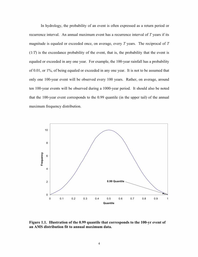
In hydrology, the probability of an event is often expressed as a return period or

recurrence interval. An annual maximum event has a recurrence interval of T years if its

magnitude is equaled or exceeded once, on average, every T years. The reciprocal of T

(1/T) is the exceedance probability of the event, that is, the probability that the event is

equaled or exceeded in any one year. For example, the 100-year rainfall has a probability

of 0.01, or 1%, of being equaled or exceeded in any one year. It is not to be assumed that

only one 100-year event will be observed every 100 years. Rather, on average, around

ten 100-year events will be observed during a 1000-year period. It should also be noted

that the 100-year event corresponds to the 0.99 quantile (in the upper tail) of the annual

maximum frequency distribution.

Figure 1.1. Illustration of the 0.99 quantile that corresponds to the 100-yr event of an AMS distribution fit to annual maximum data.

0

2

4

6

8

10

0 0.1 0.2 0.3 0.4 0.5 0.6 0.7 0.8 0.9 1Quantile

Freq

uenc

y

0.99 Quantile

5

Data for frequency analysis studies can be compiled in several ways. An annual

maximum series (AMS) includes only the largest event in each year, while a partial

duration series (PDS), or peaks-over-threshold (POT) series, includes all events above a

truncation level or threshold. It is assumed that all samples used are independent and

identically distributed. A PDS with an equal number of peaks as its corresponding AMS

is referred to as an annual exceedance series. While the assumption of independence is

usually valid for AMS data, a drawback of the AMS is that it only accounts for the largest

event in each calendar year, regardless of whether the second event in a year exceeds the

largest events of other years. On the other hand, while long and reliable PDS records are

often available, it is difficult to specify criteria for defining independent peaks and

determining an appropriate threshold value.

Traditionally, frequency analysis studies have derived estimates from at-site data

and have created isopluvial maps from these site-specific estimates using interpolation

procedures and judgement. Since the record lengths are often relatively short at gaged

sites, regionalization techniques are now used to increase accuracy. Regional frequency

analysis “trades space for time” by using data from nearby or similar sites to derive

estimates for any given site in a homogeneous climatic region (Stedinger et al., 1993).

A common method for pooling summary statistics from different sites is the index

flood procedure. The term “index flood” comes from early studies (e.g., Dalrymple,

1960) that used flood data when implementing the procedure. The main assumption of

an index flood procedure is that the sites in a homogeneous region have an identical

frequency distribution apart from a site-specific scaling factor, the index flood. For

6

simplicity, the index flood is usually the mean of the site-specific data (Hosking and

Wallis, 1997).

The methodology used for deriving rainfall IDF estimates for this study is an

index flood based regional frequency analysis approach outlined by Hosking and Wallis

(1997). Rather than using traditional methods (i.e., method of moments or maximum

likelihood procedures) for compiling site-statistics and estimating distribution

parameters, L-moments are used. L-moments are expectations of certain linear

combinations of order statistics (Hosking, 1990) that have been found in many cases to

be more efficient and robust than conventional estimation methods.

The first step in this regional frequency analysis approach is to screen the data for

gross errors and inconsistencies. The second is to identify homogeneous regions, within

which all sites are assumed to have an identical frequency distribution apart from a site-

specific scaling factor. It is stressed that delineation of homogeneous regions should be

based on site characteristics (e.g., latitude, longitude and elevation) rather than site

statistics as homogeneity is tested against site statistics and it would compromise the

integrity of the test if site statistics were used both for delineation and for testing

(Hosking and Wallis, 1997). The third step is to choose a frequency distribution that not

only fits the observed data well, but also yields robust quantile estimates. The fourth and

final step is to estimate the regional frequency distribution by combining the weighted at-

site parameter estimates to obtain regional parameter estimates. In this study,a procedure

known as the regional L-moment algorithm is used (Hosking and Wallis 1997). Quantile

estimates at a site are then obtained by multiplying the regional quantiles by the index

flood. In this study, the index flood is spatially interpolated using geostatistical methods.

7

2.0 RELATED STUDIES

2.1 Previous Studies

Since Yarnell’s seminal publication 65 years ago (Yarnell, 1935), rainfall frequency

analysis has evolved substantially due to the advent of computers, increased data

availability, and the development of more efficient and robust statistical procedures.

Traditionally, annual maximum series data has been fit to a distribution using method-of-

moments parameter estimators to obtain quantile estimates at a site, and contours have

been drawn subjectively or semi-analytically through the point estimates to obtain

regional estimates. In more recent studies (e.g., Julian et al., 1999), a regional frequency

analysis procedure using L-moments, which are based on probability-weighted moments

(Hosking and Wallis, 1997), has been used with regional information to yield more

objective and robust quantile estimates for a region. The following is a brief review of

the methodologies used in other relevant rainfall frequency studies.

The U.S. Weather Bureau’s Technical Paper 25 (1955) presented a set of rainfall

IDF curves for 203 U.S. Weather Bureau stations, 10 of which are in Michigan. TP-25

provided estimates for durations ranging from 5 minutes to 24 hours, and for recurrence

intervals of 2 to 100 years. The Gumbel distribution was fit to annual maximum series

data using method-of-moments parameter estimators to derive quantile estimates for each

gaged site. These annual series quantile estimates were then transformed to partial

duration series values by multiplying by a frequency-dependent empirical factor. For

estimating rainfall intensities at ungaged sites, it was recommended that IDF relationships

be derived using local data.

8

Technical Paper 40 (Hershfield, 1961) was an outgrowth of several previous

Weather Bureau publications that were prepared under the direction of Hershfield,

including TP-25. Rainfall IDF estimates used in design up to this point largely came

from Yarnell’s study (1935), which lacked sufficient data. TP-40 supplied estimates for

durations ranging from 30 minutes to 24 hours and recurrence intervals of 1 to 100 years

for the continental United States. Method of moments parameter estimators were again

used to fit the Gumbel distribution to annual maximum series data (through 1958) and

derive quantile estimates for the 2- and 100-year recurrence intervals for each gaged site.

A recurrence interval diagram was used in conjunction with these quantile estimates for

estimating values for other frequencies. The line spacing on the diagram was both

empirically and theoretically derived. For return periods from 1 to 10 years, the spacing

is based on empirical freehand curves drawn through plots of partial duration series data.

For return periods from 20 to 100 years, the spacing was derived from fitting annual

maximum series data to the Gumbel distribution. As in TP-25, the annual series quantile

estimates were transformed to partial duration series values by multiplying by a

frequency-dependent empirical factor. Because of the arbitrary beginning and ending of

a clock hour or calendar day, other empirical factors were also applied to convert from

clock-time to actual (time-correct) values. For IDF estimation at ungaged sites,

isopluvial maps where constructed for the entire United States, based on the derived at-

site IDF estimates.

In the 1970’s it was found that the ratios for shorter durations in TP-40 did not hold

true for different recurrence intervals. In addition, an increased demand for hydrologic

planning and design for small watersheds prompted the National Oceanic and

9

Atmospheric Administration (NOAA) to update TP-40 for short durations. NOAA

Technical Memorandum NWS Hydro-35 (Hydro-35) (Frederick et al., 1977) provided

IDF estimates for durations from 5 to 60 minutes and for return periods from 2 to 100

years for the Eastern and Central United States. The Gumbel distribution was fit to

annual maximum series data (through 1972) using method of moments parameter

estimators to derive quantile estimates for each gaged site. Equations and nomograms for

intermediate duration and return period interpolations were provided. As in the previous

two studies, annual series quantile estimates were converted to partial duration series

values by multiplying by a frequency-dependent empirical factor. As in TP-40, to adjust

clock-time results to actual (time-correct) results, a previously derived empirical factor

was verified and applied to the resulting IDF estimates. A space-averaging algorithm

applied to the at-site IDF estimates was then used in creating isopluvial maps.

More recent studies have been justified on the grounds that the above publications no

longer supplied reliable rainfall IDF values, which has been largely attributed to their

lack of spatial resolution to adequately depict local variations in rainfall. Other State

highway departments (e.g., Dunn, 1986) and agencies (Huff and Angel, 1989; Sorrell and

Hamilton, 1990; Huff and Angel, 1992) have deemed it necessary to conduct

independent, state- or regional-specific frequency analysis projects.

For Pennsylvania (Dunn, 1986), five regional-specific IDF curves were developed

which provided estimates for durations ranging from 5 minutes to 24 hours, and for

recurrence intervals of 1.01 to 100 years. Method-of-moments parameter estimators were

used to fit partial duration series data (through 1983) to the Log-Pearson Type III

distribution to derive quantile estimates at each gaged site. For ungaged sites, five

10

regions of similar rainfall intensity were delineated. A representative gage from each

region was chosen, based on its similarity to the average log-Pearson values of other

gages in the region. An IDF curve was then constructed for the chosen gage and applied

to its respective region.

To update TP-40 for 24-hour storms in Michigan, Sorrell and Hamilton (1990)

developed IDF estimates for recurrence intervals of 2 to 100 years. The Gumbel

distribution was fit to annual maximum series data using method-of-moments parameter

estimators to derive quantile estimates at each gaged site. Daily rainfall data were used,

with the majority of the records through 1980, except for 15 gages with data through

1987 to incorporate a large event observed in September 1986. As in TP-40 and other

studies, analysis results were multiplied by a frequency-specific empirical factor to

convert annual series to partial duration series results, and an additional factor was

applied to convert clock-time values to corresponding time-correct values. Isopluvial

maps were constructed for each recurrence interval using the at-site IDF estimates. It

should be noted that the current MDOT rainfall frequency zones appear to follow these

contours.

In an extension of Bulletin 70 (Huff and Angel, 1989), Bulletin 71 (Huff and Angel,

1992) updated IDF estimates for nine States in the Midwest (including Michigan) for 1-

hour to 10-day durations and for recurrence intervals of 2 months to 100 years. The main

motivation for this study stemmed from the need to update TP-40 for the region. In

addition, an apparent climatic trend was deemed to have affected the frequency

distributions of extreme rainstorms in Illinois from 1901-1980 (Huff and Changnon,

11

1987). This was later confirmed by Huff and Angel (1990) for other portions of the

Midwest.

In Bulletin 71, three procedures for fitting the daily annual maximum series data

(through 1986) were examined. The methods of L-moments and maximum likelihood

were used to fit the data to the Generalized Extreme Value (GEV) distribution. The

results of these analyses were compared to a log-log graphical analysis, which the authors

refered to as the Huff-Angel method. The Huff-Angel method involves plotting the

logarithm of rainfall amounts versus the logarithm of the recurrence intervals and fitting a

line through the data points to extrapolate values at higher frequencies at each gaged site.

Although this method is more subjective than using other statistical methods, Huff and

Angel suggested that the log-log plots allow the analyst to take meteorological and

climatological knowledge into consideration. Extrapolation for this method is cut off at

or near the 100-year recurrence interval, since the data are not fit to a specific theoretical

distribution. The authors stated that the traditional method of moments procedure was

not used due to its relatively poor performance compared to L-moments and maximum

likelihood.

Since the method of L-moments was based on a regional approach, the stations in

each State were grouped according to the National Weather Service (NWS) climate

divisions as shown in Figure 2.1 (with the exception of Indiana and Minnesota, where

some regrouping of stations was necessary due to high regional heterogeneity and station

discordancy). These divisions have been traditionally accepted as areas of homogeneous

climate. Indiana and Minnesota were chosen for comparison of the three methods (GEV

12

with L-moments, GEV with maximum likelihood, and the Huff-Angel method), because

of their diverse

Figure 2.1. NWS divisions of homogeneous climate for the Midwest (Huff and Angel, 1992).

climatic features. After comparing estimates it was found that each method provided

results that did not vary significantly from a statistical or meteorological point of view.

Overall, the Huff-Angel estimates were between those of the other two procedures. Upon

13

comparing isopluvial maps, it was concluded that the Huff-Angel spatial patterns better

conformed to climatological knowledge of the distribution of rainfall in the Midwest.

Because only daily rainfall data were analyzed, ratios were derived to convert 24-

hour values to shorter durations (5 minutes to 18 hours). These ratios were derived using

36 years of data from 34 Illinois stations, plus 21 stations from bordering states, and were

found to be in close agreement with those developed in TP-40. Duration-specific

empirical ratios to estimate intensities for less than the 2-year return period were also

provided. The resulting Huff-Angel IDF estimates were then converted from annual

series to partial duration series values by multiplying by a duration and frequency-

specific factor. Additional duration-specific empirical factors were applied to convert

from clock-time to time-correct values. To provide IDF estimates at ungaged sites,

isopluvial maps were created from the at-site frequency estimates. For presenting IDF

estimates in tabular form, areal mean values were computed for each NWS climate

division in each state. Average frequency distributions were developed using all stations

within a division and those in surrounding divisions near its boundaries.

More recently, in a report prepared for the Southeastern Wisconsin Regional

Planning Commission (SEWRPC), Loucks et al. (2000) updated IDF estimates for

durations of 5 minutes to 240 hours and for 2- to 100-year recurrence intervals for 7

counties in and around the Milwaukee area. Due to gage relocation and concern about

climate change, several tests for trends and data homogeneity were performed on data

compiled at the Milwaukee WSO (Weather Service Office) gage. No evidence was

found of any such trends in the data. On account of the complete, high quality, long

duration data for the Milwaukee WSO gage, at-site analysis formed the primary basis of

14

their study. In addition, a regional analysis was undertaken using data from the

Milwaukee gage and 14 surrounding gages to supplement the at-site analysis. All

frequency analysis procedures were performed on annual maximum series data.

The Generalized Extreme Value (GEV) distribution was fit to the at-site

Milwaukee data using the method of L-moments. The regional analysis was then

performed following the procedure developed by Hosking and Wallis (1997). The seven-

county area was treated as one homogeneous region, and the GEV distribution provided

the best fit to the regional data. Analyses were carried out on data for the full period of

record (1890’s – 1998), and for the period from 1940-1998. The resulting quantile

estimates were compared for the four scenarios (i.e., at-site and regional analysis for both

time periods). As a whole, the full period of record at-site estimates were smallest, while

the at-site 1940-1998 estimates were largest (due in part to an outlying event that

occurred in August 1986), with the regional estimates in between. It was recommended

that the at-site GEV quantile estimates for the full period of record be used for design

rainfall for the Southeastern Wisconsin Region. This was mainly due to the regional

analysis providing lower estimates than recent observations at Milwaukee. In TP-40,

estimates were converted from annual series to partial duration series values by

multiplying by a frequency-specific, empirically derived value, and additional factors

were used to convert short-duration clock-time estimates to actual (time-correct) values.

15

2.2 Current Studies

Currently, the National Weather Service’s Office of Hydrology is updating TP-40

for the Ohio River Basin (Julian et al., 1998, 1999, 2000, 2001). This study encompasses

13 states and parts of 9 others, including the southern portion of Michigan. Daily, hourly,

15-minute, and N-minute data are being analyzed. Daily data, through December 2000,

was obtained from the National Climatic Data Center (NCDC), the U.S. Army Corps of

Engineers (COE), and the U.S. Geological Survey (USGS). A total of 3269 daily stations

are being analyzed, with the average record length of the stations being 56 years. Hourly

data was obtained from the COE through December 2000. There are 984 total hourly

stations being analyzed with an average record length of 42 years. Digital N-minute data

was obtained from the NCDC through December 2000 in two different data sets that were

merged into one containing a total of 76 stations. All data has undergone or is currently

undergoing quality control. Quality control includes entering the non-digital data by

hand, merging stations and deleting stations with a record length less than twenty years.

In order to merge a station, the following criteria must be met: stations must be within

100 feet elevation, be within five miles distance, and contain a gap between records of

five years or less, or an overlap in records of five years or less.

Both annual maximum and partial duration series data are being analyzed. The

partial duration series contains N peaks, with N being equal to the actual number of years

of record for that station, corresponding to the annual exceedance series. This study is

also implementing the regional frequency analysis technique using L-moments as

outlined by Hosking and Wallis (1997). The project area has been divided into 16

16

regions based on their respective “extreme precipitation climate.” Preliminary analysis

has been completed for Illinois, Indiana and Ohio. Analysis was done on each state as a

region, and then the states were combined into one region and the results compared. Five

three-parameter distributions were tested for an appropriate fit to the data: GEV

(Generalized Extreme Value), LNO (Log Normal), GLO (Generalized Logistic), GPA

(Generalized Pareto) and PE3 (Pearson Type III). Regardless of duration and region, the

best fits for the annual maximum and partial duration series data were provided by the

GEV distribution and the GNO distribution, respectively. The results of this analysis

demonstrated the effects of regionalization on frequency values. Results for Indiana and

Ohio were lower than the regional results, while those for Illinois were higher. However,

these departures from the average regional values were determined not to be significant.

A trend and shift statistical analysis was performed on the data to address

concerns about climate change on precipitation values. The analysis was performed on

annual maximum data from 2755 stations in 22 states. The data was shown to be

basically free from linear trends and shifts at a 90% confidence level. There were 1510

stations (or 84%) tested that were free from linear trends, and 437 of 531 (or 84%) tested

stations were free from shifts in the mean. Trends and shifts are only significant in about

15% of the stations.

Another important goal of this study is to develop an Internet-Based Geographical

User Interface (GUI). The GUI uses a point-and-click interface in which the area of

interest can be selected from a shaded relief map. The duration, units, and season can

also be selected, and then based on these selections, a color IDF curve and data table are

17

generated. This system is designed to manage future studies and will also have several

supporting web pages.

A published hard copy of the final report for this study is expected to be

completed in June of 2002.

18

3.0 RAINFALL DATA IN MICHIGAN

3.1 Sources and Coverage

This study utilizes 76 hourly and 152 daily rainfall-recording stations throughout

Michigan, along with 81 Southeast Michigan Council of Governments (SEMCOG) short

duration rainfall-recording stations located in 5 counties in and around the Detroit area

(see Figures 3.1 and 3.2). Annual maximum and partial duration series data for 5 to 60

minutes have been compiled from daily records, data for durations from 1 to 18 hours

have been compiled from hourly records, and the 24-hour duration data have been

compiled from daily records. Annual maximum series data was not used in the short

duration analysis as the data contain only rainfall amounts above specified thresholds.

SEMCOG recording stations have record lengths ranging from 16 to 38 years, with an

average record length of 30 years (through 1999). The hourly recording stations have

record lengths ranging from 18 to 49 years, with an average record of 41 years (through

1996). The daily recording stations have record lengths ranging from 21 to 117 years,

with an average record of 63 years (through 1996).

Sixteen hourly stations, with recording periods that do not overlap, have been

combined to increase record length. The criteria for station combination were that

stations must be within 0.07 decimal degrees of latitude and longitude and within 1000

feet in site elevation (Julian et al., 1998). The maximum elevation difference between the

stations actually combined was only 99 feet. Due to acceptable areal coverage and

adequate record lengths, daily stations were not combined.

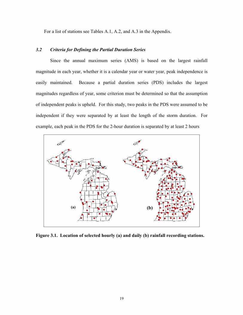
19

For a list of stations see Tables A.1, A.2, and A.3 in the Appendix.

3.2 Criteria for Defining the Partial Duration Series

Since the annual maximum series (AMS) is based on the largest rainfall

magnitude in each year, whether it is a calendar year or water year, peak independence is

easily maintained. Because a partial duration series (PDS) includes the largest

magnitudes regardless of year, some criterion must be determined so that the assumption

of independent peaks is upheld. For this study, two peaks in the PDS were assumed to be

independent if they were separated by at least the length of the storm duration. For

example, each peak in the PDS for the 2-hour duration is separated by at least 2 hours

Figure 3.1. Location of selected hourly (a) and daily (b) rainfall recording stations.

(a) (b)

20

Figure 3.2. Location of SEMCOG recording stations.

from another peak. For each duration and recording station, the number of peaks

compiled for the PDS data was 2*N, where N is the number of peaks in the AMS. The

actual number of peaks used in the PDS analysis is discussed in Chapter 5.

3.3 Conversion from Annual Maximum to Partial Duration Series Quantiles

Because the PDS can include more than one large event in any particular year, the

results from a PDS analysis are thought to be more useful for hydraulic design purposes,

especially for return periods shorter than 10 years. However, compiling and processing

PDS data is laborious compared to AMS data. In the past, to avoid PDS processing,

empirical factors were developed to convert results from an AMS analysis to PDS values.

The factors used in this study (see Table 3.1) are those developed for TP-40 (Hershfield,

1961). These factors are based on a sample of about 200 geographically well-distributed

first-order NWS stations (Frederick et al., 1977). The factors in Table 3.1 have been

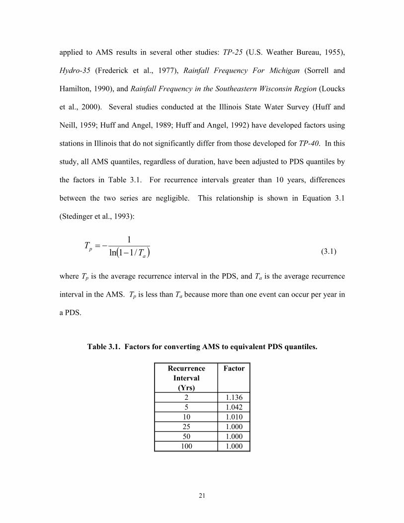
21

applied to AMS results in several other studies: TP-25 (U.S. Weather Bureau, 1955),

Hydro-35 (Frederick et al., 1977), Rainfall Frequency For Michigan (Sorrell and

Hamilton, 1990), and Rainfall Frequency in the Southeastern Wisconsin Region (Loucks

et al., 2000). Several studies conducted at the Illinois State Water Survey (Huff and

Neill, 1959; Huff and Angel, 1989; Huff and Angel, 1992) have developed factors using

stations in Illinois that do not significantly differ from those developed for TP-40. In this

study, all AMS quantiles, regardless of duration, have been adjusted to PDS quantiles by

the factors in Table 3.1. For recurrence intervals greater than 10 years, differences

between the two series are negligible. This relationship is shown in Equation 3.1

(Stedinger et al., 1993):

( )ap T

T/11ln

1−

−= (3.1)

where Tp is the average recurrence interval in the PDS, and Ta is the average recurrence

interval in the AMS. Tp is less than Ta because more than one event can occur per year in

a PDS.

Table 3.1. Factors for converting AMS to equivalent PDS quantiles.

Recurrence Interval

(Yrs)

Factor

2 1.1365 1.04210 1.01025 1.00050 1.000100 1.000

22

3.4 Adjustment of Short Duration and Daily Quantiles

The rainfall data used in this study were observed at recording stations that take a

reading once every hour (1- to 18-hour durations) or once daily (24-hour duration). Short

duration data (5-minute to 30-minute durations) are recorded by Universal Dual-Traverse

weighing type gages that produce a trace on a strip chart. An overlay is then used for the

various time increments to obtain the short duration readings. Due to the arbitrary

beginning and ending of a clock-hour or calendar day, only a portion of a true 5-minute,

1-hour, or 24-hour storm may be observed. To account for the likely failure of observing

a storm’s true rainfall (or duration), empirical factors are applied to quantiles from a

frequency analysis. The factors in Table 3.2 for the 1-, 2-, and 3-hour durations are taken

from Loucks et al. (2000). Their findings are based on an analysis of three NWS first-

order stations (Green Bay, Madison and Milwaukee). The factor in Table 3.2 for the 24-

hour duration is taken from Huff and Angel (1992), who conducted a study for the

Midwest based solely on daily data. Others who have derived and used similar values as

those in Table 3.2 are Huff and Neill (1959), Hershfield (1961), Frederick et al. (1977),

Huff and Angel (1989), and Sorrell and Hamilton (1990). Both AMS and PDS quantiles

derived in this study have been adjusted by the factors in Table 3.2 to reflect actual (time

correct) values. The effects of event truncation are negligible for the 4- to 18-hour

durations, when using hourly data. It is assumed that the effects of event truncation are

also negligible for the 30-minute duration when using 5-minute data.

23

Table 3.2. Factors for converting clock-hour quantiles to actual (time-correct) quantiles.

Duration(hours)

Factor

5 min 1.1310 min 1.0415 min 1.02

1 1.132 1.043 1.0224 1.13

24

4.0 TRENDS IN MICHIGAN RAINFALL DATA

4.1 Background

A typical assumption in any frequency analysis study is that the observed records

are stationary over time. That is, year-to-year variations in the data are expected, but the

time series does not exhibit major temporal fluctuations or long-term trends. This

assumption allows the use of all available historical data with equal weight.

A positive trend over time in rainfall data could have serious design implications.

For example, a structure that was designed on the basis of a 10-year event may actually

be subject to this event once every 5 years. Recent studies conducted at the Illinois State

Water Survey (Huff and Angel, 1990; Angel and Huff, 1997) have investigated trends in

rainfall for nine Midwestern States, including Michigan. Angel and Huff (1997)

concluded that stations in the Midwest were more likely to experience severe one-day

rainfall events (> 2 inches) in more recent years. An analysis of the geographic

distribution of changes in the annual maximum series data showed areas of increases

across the Midwest. In light of these and other findings (Karl et al., 1996; Karl and

Knight, 1998; and Kunkel et al., 1999), trend analysis of annual maximum and partial

duration series data for Michigan is discussed here.

4.2 Identifying Trends in the Annual Maximum Series

To determine if there has been a shift in the mean of the daily annual maximum

series (AMS) over the last 48 years, a non-parametric rank-sum test (e.g., Hirsch et al.,

1993) was performed on 27 daily recording stations with least 96 years of record. A non-

parametric method was chosen because the data are not assumed to follow a specified

25

distribution (e.g., most parametric tests assume that data are normally distributed). The

data were divided into two 48-year periods, 1901-48 and 1949-96. Several rainfall values

at each station had the same magnitude for different years, which resulted in tied ranks.

This is accounted for in the formulation of the rank-sum test (e.g., Hirsch et al., 1993).

The null hypothesis tested (H0) was that the second group (1949-96) does not contain

larger values than the first group. The results of this analysis show that 22 of the 27 daily

recording stations tested have larger annual maximum values from 1949-96. Three

stations showed increases at significance levels of p = 0.15, one at p = 0.20, and five at p

= 0.25 (one-sided hypothesis test)1. At the remaining stations increases were less

significant. Five of the 27 stations showed decreases. The spatial distribution of results

is shown in Figure 4.1. Because 81% of the stations tested have experienced increases

over time, further evaluation was deemed necessary.

For the 27 daily recording stations, the data were again divided into two 48-year

periods, 1901-48 and 1949-96. The Gumbel distribution and method of moments

estimators were used to derive the 2-year 24-hour (one-day) values from the two different

recording periods for each station. It can be seen from Figure 4.2 that the results derived

from the 1949-96 data are larger than those derived from the 1901-48 data for 22 of the

27 stations.

In order to investigate a trend in the daily AMS data for all 152 daily recording

stations, a plot was made of the daily means from the full period of record versus the

daily means from 1949-96. Figure 4.3 shows that the daily AMS means for 1949-96 are

consistently larger than those from the full period of record. The results of the analyses

1 The significance level p can be considered the probability of erroneously rejecting hypothesis H0. In other words, there is probability p that the more recent data has larger values due to sampling variability alone.

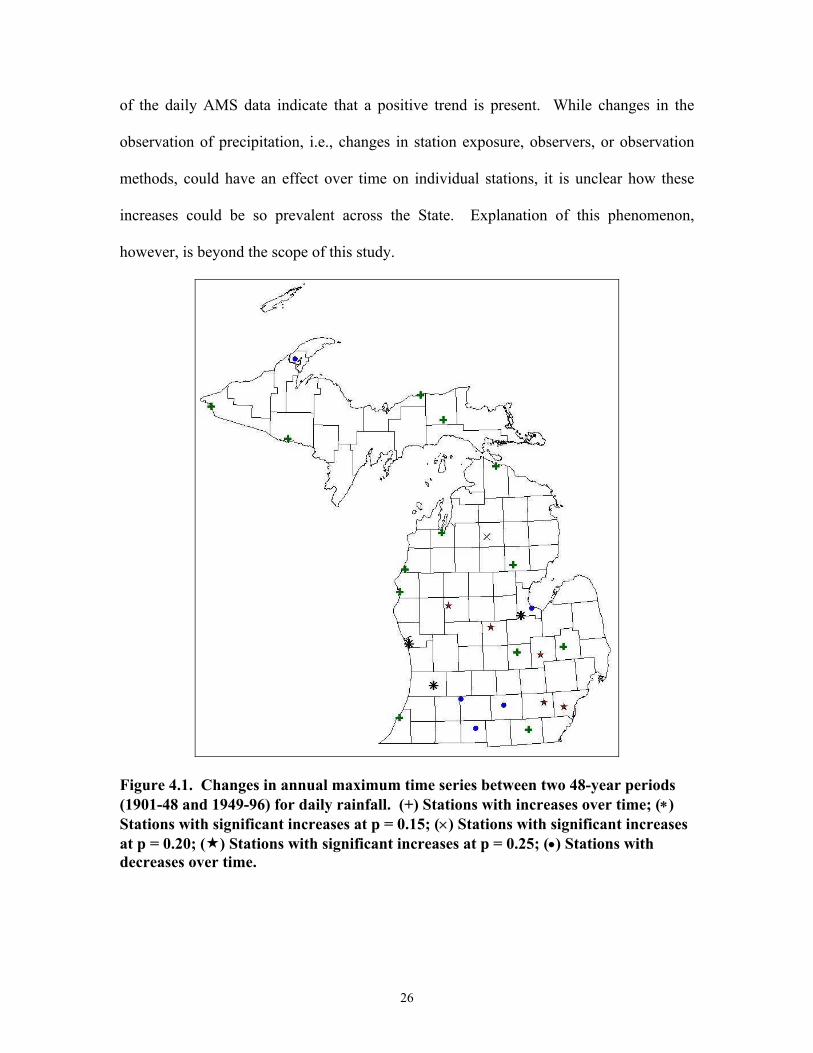
26

of the daily AMS data indicate that a positive trend is present. While changes in the

observation of precipitation, i.e., changes in station exposure, observers, or observation

methods, could have an effect over time on individual stations, it is unclear how these

increases could be so prevalent across the State. Explanation of this phenomenon,

however, is beyond the scope of this study.

Figure 4.1. Changes in annual maximum time series between two 48-year periods (1901-48 and 1949-96) for daily rainfall. (+) Stations with increases over time; (∗) Stations with significant increases at p = 0.15; (×) Stations with significant increases at p = 0.20; ( ) Stations with significant increases at p = 0.25; (•) Stations with decreases over time.

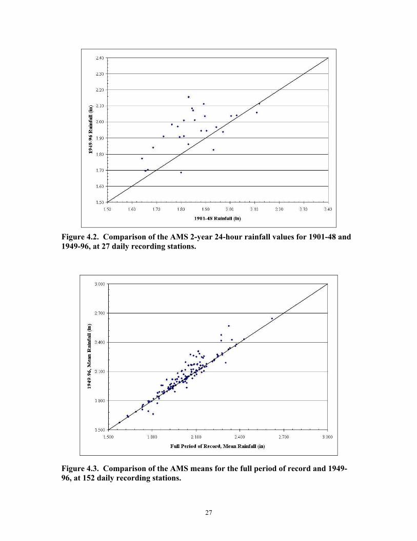
27

Figure 4.2. Comparison of the AMS 2-year 24-hour rainfall values for 1901-48 and 1949-96, at 27 daily recording stations.

Figure 4.3. Comparison of the AMS means for the full period of record and 1949-96, at 152 daily recording stations.

28

The increase in the daily AMS data over time presents a challenge to estimating

rainfall values for different recurrence intervals. If the entire period of record is used,

there may be an underestimation of (future) rainfall IDF values. However, if estimates

are derived using only observations from the latter part of the century (1949-96),

important data for estimating intensities with longer recurrence intervals (i.e., the 100-

year event) are lost. To address this problem, Huff and Angel (1989) weighted the

expected rainfall amounts for the 1901-83 period by a factor calculated as the ratio of the

1941-80 rainfall IDF estimates to those for the entire 1901-83 period at each of 61

stations in Illinois. Mean ratios were then calculated for each of the 10 NWS climatic

zones in Illinois, and these average values were used to adjust the station values derived

from the 1901-83 data. Average ratios were used to reduce the effect of random

sampling fluctuations between the 61 individual stations. Huff and Angel (1989)

rationalized that this procedure allowed, for example, for the 100-year event to be derived

using all available information, while still taking into account the observed trend.

Because a positive trend has been identified in the daily AMS data for Michigan, similar

adjustment may be necessary to put greater weight on the more recent rainfall events.

Similar tests were conducted on 25 hourly recording stations with at least 46 years

of record for the 1- and 12-hour durations. A rank-sum test (e.g., Hirsch et al., 1993)

was conducted, identical to that performed on the daily data. The 1- and 12-hour data

were divided up into two groups, 1951-73 and 1974-96. The results of the rank-sum test

for the 1-hour duration showed that 19 of the 25 hourly recording stations tested have

observed lower values from 1974-96; while only six stations showed increases in the

29

values observed (two at p = 0.25). The results for the 12-hour duration are similar, with

16 stations showing decreases in the values observed and just nine stations showing

increases (three at p = 0.20).

To further investigate the possibility of a trend being present in the hourly data, a

quantile comparison was performed. The Gumbel distribution and method of moments

estimators were used to derive 2-year rainfall estimates from data for the full period of

record (1951-96) and from 1974-96. The plots in Figures 4.4 and 4.5 show that the 2-

year estimates from the last half of the recording period are not larger than those from the

full period of record.

Figure 4.4. Comparison of the AMS 2-year 1-hour rainfall values for the full period of record (1951-96) and 1974-96, at 25 hourly recording stations.

30

Figure 4.5. Comparison of the AMS 2-year 12-hour rainfall values for the full period of record (1951-96) and 1974-96, at 25 hourly recording stations.

The results of the rank-sum test and the quantile comparison for the 1- and 12-

hour durations have shown that no positive trend is present in the hourly data.

Furthermore, since all of the hourly data are from the last half of the century (1948-96), it

is deemed that this data represents current Michigan rainfall frequency estimates and can

be treated with equal weight to produce reliable IDF estimates for the 1- to 18-hour

durations.

4.3 Identifying Trends in the Partial Duration Series

To investigate the possibility of trends in the partial duration series (PDS) data, a trend

analysis was conducted on daily, hourly, 10- and 30-minute data. For the daily data, a

time series of the number of rainfall events that exceeded 2 inches or more and 4 inches

or more were plotted and analyzed (see Figures 4.6 and 4.7). These figures are based on

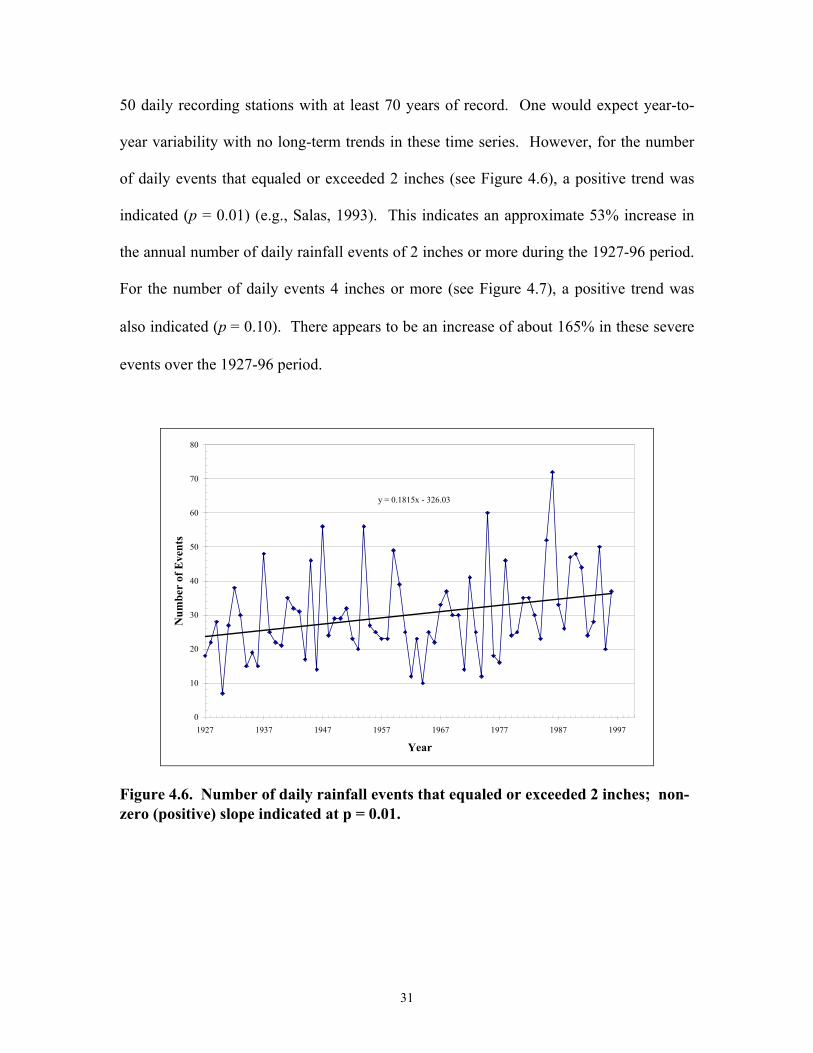
31

50 daily recording stations with at least 70 years of record. One would expect year-to-

year variability with no long-term trends in these time series. However, for the number

of daily events that equaled or exceeded 2 inches (see Figure 4.6), a positive trend was

indicated (p = 0.01) (e.g., Salas, 1993). This indicates an approximate 53% increase in

the annual number of daily rainfall events of 2 inches or more during the 1927-96 period.

For the number of daily events 4 inches or more (see Figure 4.7), a positive trend was

also indicated (p = 0.10). There appears to be an increase of about 165% in these severe

events over the 1927-96 period.

y = 0.1815x - 326.03

0

10

20

30

40

50

60

70

80

1927 1937 1947 1957 1967 1977 1987 1997

Year

Num

ber

of E

vent

s

Figure 4.6. Number of daily rainfall events that equaled or exceeded 2 inches; non-zero (positive) slope indicated at p = 0.01.

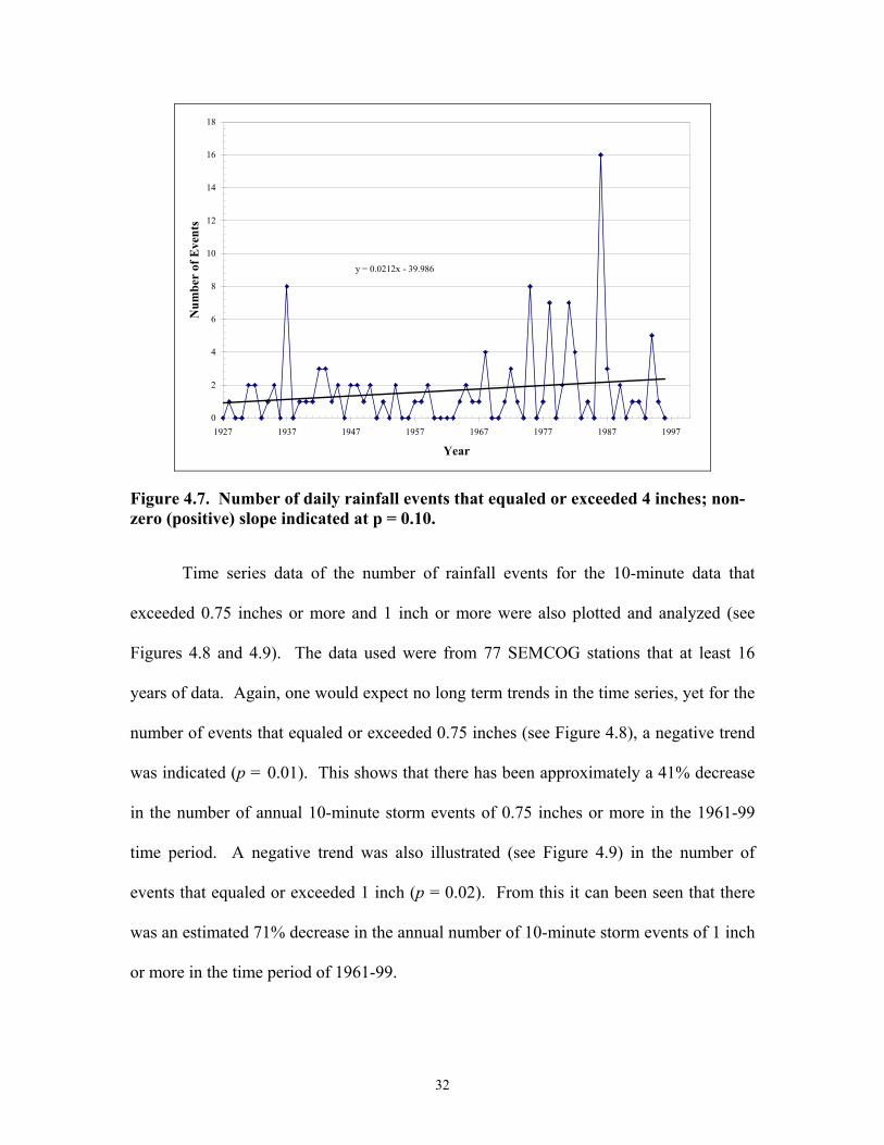
32

y = 0.0212x - 39.986

0

2

4

6

8

10

12

14

16

18

1927 1937 1947 1957 1967 1977 1987 1997

Year

Num

ber

of E

vent

s

Figure 4.7. Number of daily rainfall events that equaled or exceeded 4 inches; non-zero (positive) slope indicated at p = 0.10.

Time series data of the number of rainfall events for the 10-minute data that

exceeded 0.75 inches or more and 1 inch or more were also plotted and analyzed (see

Figures 4.8 and 4.9). The data used were from 77 SEMCOG stations that at least 16

years of data. Again, one would expect no long term trends in the time series, yet for the

number of events that equaled or exceeded 0.75 inches (see Figure 4.8), a negative trend

was indicated (p = 0.01). This shows that there has been approximately a 41% decrease

in the number of annual 10-minute storm events of 0.75 inches or more in the 1961-99

time period. A negative trend was also illustrated (see Figure 4.9) in the number of

events that equaled or exceeded 1 inch (p = 0.02). From this it can been seen that there

was an estimated 71% decrease in the annual number of 10-minute storm events of 1 inch

or more in the time period of 1961-99.

33

Figure 4.8. Number of 10-minute rainfall events that equaled or exceeded 0.75 inches; negative slope indicated at p = 0.1.

Figure 4.9. Number of 10-minute rainfall events that equaled or exceeded 1 inch; negative slope indicated at p = 0.02

y = -0.1694x + 348.63

0

5

10

15

20

25

30

35

40

1955 1960 1965 1970 1975 1980 1985 1990 1995 2000 2005

Year

Num

ber o

f Eve

nts

y = -0.0779x + 157.03

0

2

4

6

8

10

12

1955 1960 1965 1970 1975 1980 1985 1990 1995 2000 2005

Year

Num

ber o

f Eve

nts

34

This trend was also seen in the analysis of the 30-minute data. For the 30-minute

duration, plots were made of the data that equaled or exceeded 1.75 inches and the data

that equaled or exceeded 2 inches (see Figures 4.10 and 4.11). Once again, a negative

trend was indicated by the data (p = 0.306 for 1.75 inches, p = 0.258 for 2 inches). From

this, it appears that there was a 26% decrease in the annual number of 30-minute storm

events of 1.75 inches or more and a 35% decrease in the annual number of 30-minute

storm events of 2 inches or more for the period of 1961-99.

Figure 4.10. Number of 30-minute rainfall events that equaled or exceeded 1.75 inches; negative slope indicated at p = 0.306

y = -0.0147x + 31.179

0

1

2

3

4

5

6

7

8

9

10

1955 1960 1965 1970 1975 1980 1985 1990 1995 2000 2005

Year

Num

ber o

f Eve

nts

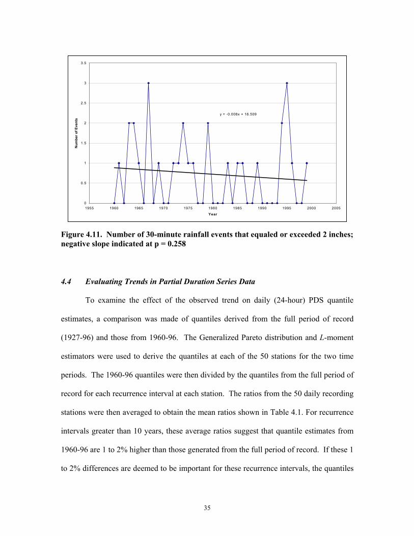
35

Figure 4.11. Number of 30-minute rainfall events that equaled or exceeded 2 inches; negative slope indicated at p = 0.258

4.4 Evaluating Trends in Partial Duration Series Data

To examine the effect of the observed trend on daily (24-hour) PDS quantile

estimates, a comparison was made of quantiles derived from the full period of record

(1927-96) and those from 1960-96. The Generalized Pareto distribution and L-moment

estimators were used to derive the quantiles at each of the 50 stations for the two time

periods. The 1960-96 quantiles were then divided by the quantiles from the full period of

record for each recurrence interval at each station. The ratios from the 50 daily recording

stations were then averaged to obtain the mean ratios shown in Table 4.1. For recurrence

intervals greater than 10 years, these average ratios suggest that quantile estimates from

1960-96 are 1 to 2% higher than those generated from the full period of record. If these 1

to 2% differences are deemed to be important for these recurrence intervals, the quantiles

y = -0.008x + 16.509

0

0.5

1

1.5

2

2.5

3

3.5

1955 1960 1965 1970 1975 1980 1985 1990 1995 2000 2005

Year

Num

ber o

f Eve

nts

36

from the full period of record could be increased by these ratios. However, for the

purposes of this study, the noted differences in quantiles were deemed to be insignificant.

Therefore, for the daily PDS, no measure will be taken to place more weight on

observations recorded in the latter years of the century.

Table 4.1. Mean ratios of 1960-96 quantiles over those from the full period of record (1927-96), derived from daily PDS data at 50 daily recording stations.

Recurrence

Interval (Yrs)

Mean Ratio

2 1.005 1.00

10 1.0125 1.0150 1.02

100 1.02

To investigate trends in the hourly PDS data, a quantile estimate comparison was

made for the 1- and 12-hour durations. Again, the Generalized Pareto distribution and L-

moment estimators were used to derive quantiles for 25 hourly recording stations for two

time periods. Ratios were then calculated by dividing quantile estimates derived from

1974-96 data by those derived from the full period of record (1951-96). The ratios were

then averaged to obtain the mean ratios shown in Tables 4.2 and 4.3. The mean ratios for

the 1-hour duration (Table 4.2) show that the quantile estimates from 1974-96 do not

differ from those generated from the full period of record. The mean ratios for the 12-

hour duration (Table 4.3) do not show a difference for recurrence intervals less than or

equal to 25 years. However, for the 50- and 100-year recurrence intervals, the estimates

for 1974-96 were 5% and 8% larger, respectively, than the values derived from the full

37

period of record. Although this may be cause for concern, these differences can easily be

attributed to sampling variability, or the uncertainty in quantile estimation for such rare

events.

Table 4.2. Mean ratios of 1974-96 quantiles over those from the full period of record (1951-96), derived from 1-hour PDS data at 25 hourly recording stations.

Recurrence

Interval (Yrs)

Mean Ratio

2 0.995 0.99

10 0.9925 0.9950 1.00

100 1.01

Table 4.3. Mean ratios of 1974-96 quantiles over those from the full period of record (1951-96), derived from 12-hour PDS data at 25 hourly recording stations.

Recurrence

Interval (Yrs)

Mean Ratio

2 0.995 0.99

10 1.0025 1.0250 1.05

100 1.08

Trends were also investigated in the short duration data by making a quantile

estimate comparison for the 10- and 30-minute data. As in the daily and hourly

comparisons, the Generalized Pareto distribution and L-moment estimators were used to

derive quantiles for 75 SEMCOG short duration stations for two time periods. The full

38

period of record for the short duration stations is from 1961-99. A comparison was made

of the quantiles from the full period (1961-99) and from a more recent period (1980-99)

by dividing the quantile estimates calculated from the 1980-99 data by the full period of

record (1961-99) data. An average was then taken of the ratios to calculate the mean

ratios that can be seen in Tables 4.4 and 4.5. The mean ratios for the 10-minute duration

(Table 4.4) show that the quantile estimates from 1980-99 are slightly less than the

quantile estimates for the full period. In fact, the 1980-99 estimates are about 6% smaller

for the 50- and 100-year recurrence intervals. A similar trend can be seen in the mean

ratios for the 30-minute duration data (Table 4.5). Again the quantile estimates from

1980-00 are slightly less than the quantile estimates for the full period. The greatest

difference between the two is that the 1980-99 estimate is about 5% smaller than the full

period estimate for the 50- and 100-year recurrence intervals.

RecurrenceInterval

(Yrs)

MeanRatio

2 0.985 0.9710 0.9625 0.9550 0.94100 0.94

Table 4.4. Mean ratios of 1980-99 quantiles over those from the full period of record (1961-99), derived from 10-minute PDS data at 75 SEMCOG stations.

39

It must be noted, for the quantile estimates derived from the 1974-96 data, that

only 23 years of data were used to derive estimates for the 50- and 100-year recurrence

intervals for these hourly comparisons. Because of the short record length, a large

amount of variability is present in estimating these values. This also holds true for the

quantile estimates derived from the 1980-99 data. For the 12-hour duration, several large

events where recorded in 1978 and 1987 at the 25 hourly stations. Because of the data

split (1951-73 and 1974-96), these large events were given greater weight, thus

contributing to the increases at the 50- and 100-year recurrence intervals noted in Table

4.3. Taking these considerations into account, and recognizing that there were no

significant differences in the quantile estimates generated from the daily and 1-hour PDS

data, no measures are taken place more weight on observations from the latter portion of

the recording period for the hourly PDS data. For the short duration data, the quantile

estimates were actually less for the 1980-99 period, therefore no weighting was needed

for the latter portion of the recording period.

Recurrence Interval

(Yrs)

Mean Ratio

2 0.985 0.9710 0.9725 0.9650 0.95100 0.95

Table 4.5. Mean ratios of 1980-99 quantiles over those from the full period of record (1961-99), derived from 30-minute PDS data at 75 SEMCOG stations.

40

4.5 Summary

The purpose of this chapter was not to speculate about global or regional climate

change, but rather to identify trends in Michigan rainfall data and account for those trends

in rainfall IDF estimation. Analyses indicate a positive trend over time in the daily AMS

data. It is recognized that some adjustment may be necessary to put greater weight on the

more recent daily rainfall events. Little evidence of such trends was identified in the

hourly AMS data; therefore no adjustments are deemed necessary. A negative trend over

time was indicated in the short duration (10- and 30-minute data).

A temporal analysis of the daily PDS data revealed significant increases in the

frequency of heavy rainfall in Michigan over a 70-year period (1927-96). In light of this,

quantile estimates derived from the 1960-96 period were compared with those derived

from the full period of record. No significant differences were found. As a result, no

measures will be taken to account for the trend in the daily PDS data. To identify trends

in the hourly PDS data, a quantile comparison was again conducted. For the 1- and 12-

hour durations, quantile estimates derived from the 1974-96 period were compared with

those derived from the full period of record, and significant differences were observed at

the 50- and 100-year recurrence intervals for the 12-hour duration. However, taking into

account sampling variability, and the fact that there were no significant differences in the

daily and 1-hour quantile comparisons, these differences will not be accounted for in

rainfall IDF estimation.

Similar results were also found for the short duration data. For the 10- and 30-

minute durations, the quantile estimates derived from the 1980-99 period were found to

be lower than those from the full period of record. These differences will not be

41

accounted for in the rainfall IDF estimation, as sampling variability and the short period

of record may easily account for this difference.

42

5.0 REGIONAL RAINFALL FREQEUNCY ANALYSIS

5.1 Introduction

The methodology used for deriving rainfall IDF estimates for the State of

Michigan is an index flood based regional frequency analysis approach as outlined by

Hosking and Wallis (1997). The procedure assumes that sites from a homogeneous

region have an identical frequency distribution apart from a site-specific scaling factor.

Rather than using traditional methods (i.e., method of moments or maximum likelihood

procedures) for compiling site-statistics and estimating distribution parameters, L-

moments are used. L-moments are expectations of certain linear combinations of order

statistics (Hosking, 1990) that have been found to be more efficient and robust than

conventional estimation methods (e.g., Hosking, 1990; and Madsen et al., 1997). Two

models based on this methodology are presented: a Generalized Pareto distribution fitted

to partial duration series data (PDS/GPA Model), and a Generalized Extreme Value

distribution fit to annual maximum series data (AMS/GEV Model).

5.2 Reasons for a Regional Analysis

Traditionally, frequency analysis studies have derived estimates from at-site data

and created isopluvial maps from these site-specific estimates. Because record lengths

are often relatively short at gaged sites (i.e., it is difficult to accurately estimate a 100-

year event from 49 years of data), regionalization techniques are used to increase

accuracy. Regional frequency analysis “trades space for time” by incorporating

hydrologic data from nearby or similar sites to derive estimates for any given site in a

homogeneous region (Stedinger et al., 1993). The concept of trading space for time is

43

illustrated in Figures 5.1 and 5.2. Figure 5.1 depicts the fit of the Generalized Extreme

Value (GEV) distribution to 2-hour annual maximum rainfall data observed at the

Hancock, MI station. Figure 5.2 illustrates the fit of the GEV to 2-hour annual maximum

rainfall data observed at 10 stations in Michigan. The pooled data in Figure 5.2 allow a

much better fit of the distribution than do the data from the single site in Figure 5.1.

Because more data are included in a regional analysis, there is potential for greater

accuracy in the final quantile estimates. In addition, recent research has shown that even

when moderate regional heterogeneity is present, a regional analysis will still yield much

more accurate quantile estimates than an at-site analysis (Lettenmaier et al., 1987;

Hosking and Wallis, 1988; Potter and Lettenmaier, 1990; Hosking and Wallis, 1997). As

opposed to streamflow data, where characteristics often differ from catchment to

catchment, regionalization is easier to employ for rainfall data in regions without

substantial relief because characteristics are often uniform over a large area (Stedinger et

al., 1993). For practical purposes this is the case for Michigan.

5.3 Definition of L-moments

L-moments are defined as expectations of certain linear combinations of order

statistics (Hosking, 1990). They are analogous to conventional moments with measures

of location (mean), scale (standard deviation), and shape (skewness and kurtosis).

Because L-moments are linear combinations of the ranked observations and do not

involve squaring or cubing the observations as is done for the conventional method of

moments estimators, they are less sensitive to outliers. The L-moment estimators of the

coefficient of variation (L-CV) and skewness (L-skewness) are also nearly unbiased and

are nearly normally distributed. In contrast, the method of moment estimators of the

44

0

0.05

0.1

0.15

0.2

0.25

0.3

0.35

0 0.25 0.55 0.85 1.15 1.45 1.75 2.05 2.35 2.65 2.95 3.25 3.55 3.85 4.15 4.3

2-hour Rainfall (in)

Rel

ativ

e Fr

eque

ncy

Figure 5.1. Generalized Extreme Value probability density function (PDF), fit to histogram of 2-hour rainfall data from Hancock, MI station (n=45).

0

0.025

0.05

0.075

0.1

0.125

0.15

0.175

0.2

0.225

0.25

0.275

0.3

0 0.25 0.55 0.85 1.15 1.45 1.75 2.05 2.35 2.65 2.95 3.25 3.55 3.85 4.15 4.45 4.75 5.05 5.35 5.65

2-hour Rainfall (in)

Rel

ativ

e Fr

eque

ncy

Figure 5.2. Generalized Extreme Value probability density function (PDF), fit to histogram of 2-hour rainfall data from 10 stations in Michigan (n=408).

45

coefficient of variation and skewness are highly biased and highly variable in small

samples. Method of moments estimators also give undue weight to outliers, which can

mask the information provided by the other observations in the data set. Wallis et al.

(1974), Hosking (1990) and Hosking and Wallis (1997) discuss these issues in greater

detail. Hosking (1990) has also shown that parameter estimates obtained from L-

moments are often more accurate in small samples than those derived using maximum

likelihood procedures. For a number of hydrologic applications, L-moments are efficient

estimators of the characteristics of hydrologic data and of a distribution’s parameters

(Stedinger et al., 1993).

L-moments are derived from modifications to probability-weighted moments

(PWMs), which were developed by Greenwood et al. (1979). For a random variable X,

PWMs can be defined as (Stedinger et al., 1993)

[ ]{ },)( rr XFXE=β (5.1)

where F(X) is the cumulative distribution function (cdf) for X. PWMs are the expectation

of X multiplied by powers of F(X). Landwehr et al. (1979), Hosking et al. (1985) and

Hosking and Wallis (1987) have used PWMs as the basis of methods for estimating

parameters of probability distributions. However, PWMs are difficult to interpret directly

as measures of the scale and shape of a probability distribution. This information is

contained in linear combinations of the PWMs, or L-moments.

5.4 Sample L-moments

Population L-moments are defined for a probability distribution, but in practice

they must be estimated from an observed sample. Estimation is based on a sample of size

46

n, arranged in ascending order (i.e., x1:n < x2:n < …< xn:n is the ordered sample). L-

moment estimation begins by estimating the population probability weighted moment βr.

An unbiased estimator of βr is (Hosking and Wallis, 1997):

nj

n

rjr x

rnnnrjjjnb :

1

1

))...(2)(1())...(2)(1(∑

+=

−

−−−−−−

= (5.2)

From br the sample L-moments are given by (Hosking and Wallis, 1997):

01 b=l (5.3)

012 2 bb −=l (5.4)

0123 66 bbb +−=l (5.5)

01234 123020 bbbb −+−=l (5.6)

012345 209014070 bbbbb +−+−=l (5.7) where l1 and l2 are respectively measures of the sample mean and scale of the

distribution. The remaining L-moments are used to determine the sample L-moment

ratios, which are (Hosking and Wallis, 1997):

2ll r

rt = (5.8)

where t3 and t4 are respectively the sample L-skewness and L-kurtosis. The sample L-

coefficient of variation (L-CV) is given by (Hosking and Wallis, 1997):

.1

2l

l=t (5.9)

47

The estimators tr and t are not unbiased, but their biases are very small in moderate or

large samples (Hosking, 1990). It has been shown that they are more robust to outliers

and are more efficient than the method of moments estimators of the coefficient of

variation, skewness and kurtosis (Hosking, 1990; Hosking and Wallis, 1997).

5.5 Regional Rainfall Frequency Analysis Methodology

The following procedure is that outlined by Hosking and Wallis (1997). The

main steps are to screen the data, identify homogeneous regions, chose a frequency

distribution, and estimate the parameters of the chosen distribution. These steps are

discussed in detail below.

Screening the Data. The first step in any statistical investigation is to check that the

data are suited for the analysis. Tests for gross outliers, inconsistencies, shifts, and trends

(see Chapter 4) are ways to check the appropriateness of the data. Additionally, Hosking

and Wallis (1997) present a discordancy measure based on the L-moments of the sites’

data. The discordancy measure is a single statistic based on the difference between the L-

moment ratios of a site and the average L-moment ratios of a group of similar sites and

can be used to identify erroneous data.

The formulation of the discordancy measure is as follows (Hosking and Wallis,

1997). With N the number of sites in a region, let

[ ]T)(4

)(3

)(u iiii ttt= (5.10)

be a vector with t, t3, and t4 estimates for site i. The superscript T denotes the

transposition of a vector or matrix. Let

48

∑=

−=N

iiN

1

1 uu (5.11)

be the group average. The matrix of sums of squares and cross-products is defined as

.)uu)(uu(A T

1−−= ∑

=i

N

ii (5.12)

The discordancy statistic for site i is then given by

).uu(A)uu(31 1T −−= −

iii ND (5.13)

For a region with 15 or more sites, site i is considered discordant if Di > 3. For this study,

all regions considered contained 15 or more sites. Hosking and Wallis (1997) note that

the discordancy measure is an increasing function of the number of sites in a region

because larger regions are more likely to contain sites with large values of Di. However,

Hosking and Wallis (1997) still recommend that Di > 3 be considered discordant, since

such sites have L-moment ratios that significantly differ from the regional average.

In addition to assisting in locating abnormalities in a data set, the discordancy

measure can aid in identifying homogeneous regions. If a site is discordant in a particular

region, it could be moved to another region. However, it is recognized that a site’s L-

moments may differ from other similar sites by chance alone. An example of this is the

Beaverton Power Plant station, in which the largest 1-hour rainfall was recorded for the

State (5.02 inches). For the State as one region, its discordancy measure (Di) is 5.47.

Because such an event is deemed to have an equal chance of occurring at any other site in

the State, the site is kept as a member of the region.

49

Identifying Homogeneous Regions. The purpose of this step is to form groups of

stations that satisfy the homogeneity condition, i.e., stations with frequency distributions

that are identical apart from a station-specific scale factor. Stations can be grouped

subjectively by site characteristics (i.e., latitude, longitude, elevation, and mean annual

precipitation). For example, Schaefer (1990) defined homogeneous regions based on

mean annual precipitation for a regional frequency analysis study of annual maximum

precipitation in the State of Washington.

Stations can also be grouped objectively using cluster analysis procedures.

Cluster analysis is a multivariate statistical analysis procedure for partitioning a data set

into groups. The procedure involves assigning a data vector to each site. Sites are then

divided into groups based on the similarity of their data vectors. The data vectors can

consist of site statistics, site characteristics, or some combination of both. Hosking and

Wallis (1997) recommend basing the regionalization of sites on site characteristics alone.

This is because site characteristics are known quantities before any data are measured at

the site. If site statistics were used, sites that have observed a large outlier, for example,

could be grouped together, resulting in inaccurate quantile estimates for that region.

Furthermore, the use of site characteristics for forming regions allows the use of site

statistics to test the appropriateness of the grouped sites. Other studies implementing

cluster analysis procedures based on site characteristics are described by Fovell and

Fovell (1993), Hosking and Wallis (1996) and Bates et al., (1998).

To investigate the possibility of dividing the State into two or more homogeneous

regions, cluster analysis was performed using latitude, longitude, elevation, and mean

annual precipitation as the site characteristics. Clusters were formed using a computer

50

program developed by Hosking (1997). This program applies Ward’s method, which

tends to produce clusters containing the same number of sites. In Ward’s method the

distance between two clusters is the sum of squares of differences in common variables

between the two clusters. The clusters formed using Ward’s method are then redefined

using a K-Means clustering algorithm (Hartigan and Wong, 1979). The aim of the

algorithm is to search for a K-partition with locally optimal within-cluster sum of squares

by moving sites from one cluster to another.

In order to test the appropriateness of a group of sites, Hosking and Wallis (1997)

present a heterogeneity measure called the H-statistic. This statistic compares the

between-site variation in sample L-moments for a group of sites with what would be

expected for a homogeneous region (Hosking and Wallis, 1997). To determine what

would be expected, repeated Monte Carlo simulations of a homogeneous region with

sites having record lengths equal to those of the observed data are performed. From the

simulated values the mean and standard deviation of the chosen dispersion measure are

obtained. To compare the observed and simulated differences, the H-statistic is defined

as (Hosking and Wallis, 1997):

.ions)of simulatdeviation (standard

ions)of simulat) - (mean dispersion(observed H = (5.14)

There are three measures of the H-statistic. The first, H(1), is the standard

deviation, weighted according to record length, of the at-site L-CVs. This is deemed to

be the most important because variation in the L-CV has a much larger effect than

variation in the L-skewness or L-kurtosis on the accuracy of the final quantile estimates

(Hosking and Wallis, 1997). The second measure, H(2), is the average distance from the

51

site coordinates to the regional average on a plot of L-CV vs. L-skewness. The third

measure, H(3), is the average distance from the site coordinates to the regional average

on a plot of L-skewness vs. L-kurtosis. A region is declared “acceptably homogeneous”

if H < 1, “possibly heterogeneous” if 1 < H < 2, and “definitely heterogeneous” if H > 2.

Choosing a Frequency Distribution. In regional frequency analysis, a single frequency

distribution is fit to the data from several sites in a homogeneous region. Because the

“true” distribution of rainfall is not known, a distribution must be chosen that not only

provides a good fit to the data, but will also yield robust and accurate quantile estimates

for each site in the region.

To determine an appropriate distribution for regional quantile estimation, Hosking

and Wallis (1997) introduce another statistic called the Z-statistic. The Z-statistic, a

goodness-of-fit measure for three-parameter distributions, measures how well the

theoretical L-kurtosis of the fitted distribution matches the regional average L-kurtosis of

the observed data. The Z-statistic for a particular distribution is defined as (Hosking and

Wallis, 1997)

,)( 44R4

DIST4

DIST στ BtZ +−= (5.15) where DIST

4τ is the theoretical L-kurtosis for the candidate distribution, R4t is the regional

average L-kurtosis weighted by record length, B4 is a simulation-based value to correct

for the bias associated with estimating R4t , and σ4 is an estimate of the standard deviation

of R4t obtained from repeated simulation of a homogeneous region whose sites have the

candidate frequency distribution and identical record lengths as the observed data. The

52

fit of the distribution is declared satisfactory if |ZDIST| < 1.64. This criterion corresponds

to an acceptance of the hypothesized distribution at a confidence level of approximately

90% (Hosking and Wallis, 1997).

The candidate three-parameter distributions considered for quantile estimation for

this study were the Generalized Logistic (GLO), the Generalized Extreme Value (GEV),

the Lognormal (LN3), the Pearson Type III (PE3), and the Generalized Pareto (GPA).

Two-parameter distributions were not considered because estimates of tail quantiles can

be severely biased if the shape of the tail of the true frequency distribution is not well

approximated by the fitted distribution. The use of a distribution with more parameters,

when the parameters are estimated accurately, yields less biased estimates of quantiles in

the tails of the distribution (Hosking and Wallis, 1997).

The Regional L-Moment Algorithm. To estimate a chosen distribution’s parameters and

obtain quantile estimates, the regional L-moment algorithm was used (Hosking and

Wallis, 1997). This procedure involves fitting the chosen distribution using the method of

L-moments; its parameters are estimated by equating the population L-moments of the

distribution to the sample L-moments derived from the observed data. Next, sample L-

moment ratios from each site in a homogeneous region are weighted according to record

length and combined to give regional average L-moment ratios. Hosking and Wallis

(1997) found that averaging L-moment ratios rather than the L-moments themselves

yields more accurate quantile estimates in all cases examined. Next, the regional mean is

set equal to 1, and regional quantile estimates are derived. Final quantile estimates are

53

obtained by multiplying the regional quantile estimate by the index flood, which for this

study is the at-site estimate of the mean.

The formulation of the regional L-moment algorithm is as follows. Assume that

there are N sites in a region, with site i having record length ni, sample mean )(1il , and

sample L-moment ratios )(it , )(3

it , )(4it , and )(

5it . The regional average L-moment ratios

Rt , R3t , R

4t , and R5t , are weighted according to record lengths as given by (Hosking and

Wallis, 1997):

,11

)(R ∑∑==

=N

ii

N

i

ii ntnt (5.16)

,11

)(R ∑∑==

=N

ii

N

i

irir ntnt

5. 4, 3,=r (5.17)

Next, the regional average mean is set to 1:

.1R1 =l (5.18)

Let (.)q̂ be the quantile function of the fitted regional frequency distribution, and

let )(1il be the index flood, or the sample mean of the at-site data. The quantile estimate at

site i for nonexceedance probability F (i.e., 1-1/T) is given by (Hosking and Wallis,

1997):

).(ˆ)(ˆ )(1 FqFQ i

i l= (5.19)

54

5.6 Determination of Rainfall IDF Estimates at Ungaged Sites

To obtain rainfall IDF estimates at ungaged sites, the regional quantile estimates

derived from data at gaged sites within a region are interpolated to all ungaged sites in

that region. Specifically, the index flood, or the at-site mean values, are spatially

interpolated over the State using geostatistical methods. This allows for rainfall IDF

estimates for durations of 1, 2, 3, 6, 12, 18 and 24 hours to be determined for any location

in the State of Michigan. For durations of less than 1 hour, a procedure was devised to

extrapolate the results obtained for the SEMCOG gages. The procedure assumes that the

ratio of N-minute to 60-minute rainfall intensity is constant throughout the state. Then,

based on the estimate of N-minute rainfall intensity for a given return period in the

Detroit area, an estimate of N-minute rainfall intensity for the same return period at

another location can be estimated as:

60

60N N ii D

D

QQ QQ

=

(5.20)

where

NiQ = N-minute rainfall intensity at site i

NDQ = N-minute rainfall intensity in the Detroit area

60iQ = 60-minute rainfall intensity at site i

60DQ = 60-minute rainfall intensity in the Detroit area

55

5.7 The Partial Duration Series Model

The formulation presented in this section is for a partial duration series (PDS)

model based on the index flood regional frequency analysis procedure outlined by

Hosking and Wallis (1997). A PDS, or peaks over a threshold (POT) series, includes all

values above a truncation level or threshold. This model assumes that all values above a

threshold are Generalized Pareto (GPA) distributed, which suggests the annual maximum

values to be Generalized Extreme Value (GEV) distributed (Hosking and Wallis, 1987;

Stedinger et al., 1993; and Madsen et al., 1997). Thus, the model introduced herein is

similar to the AMS/GEV model presented in the next section. Along with these

theoretical reasons for using the GPA distribution, the GPA distribution has been

determined to provide the best fit to the PDS data empirically, as shown in Chapter 6.

It is generally assumed in a PDS analysis that the arrival of peaks is described by

a Poisson process. That is, N(t), the number of exceedances in t years, is Poisson

distributed with probability function (Madsen and Rosbjerg, 1997)

{ } ( ) )exp(!

)( tntntNP

n

λλ−== ... 2, 1, 0,=n (5.21)

where the Poisson parameter λ equals the expected number of exceedances per year. It is

also assumed that the rainfall magnitudes above the threshold are independent and

identically distributed following the GPA distribution. Criteria for independence of

events are discussed in Chapter 3.

Because more than one event can occur in a year in a PDS, the recurrence interval

of a given rainfall event estimated using the PDS, Tp, will be less than the recurrence

56

interval estimated using the AMS, Ta (denoted T elsewhere in this document). This

relationship is given by (Stedinger et al., 1993)

( ) ./11ln

1

ap T

T−

−= (5.22)

Analogous to the relationship in Equation 5.22, Rosbjerg (1985) has shown the

T-year event quantile (F) in the distribution of exceedances to be defined as

TF

λ̂11−= (5.23)

where λ̂ is an estimator of the Poisson parameter, which is defined as (Madsen and

Rosbjerg, 1997)

.ˆtN

=λ (5.24)

Madsen and Rosbjerg (1997) present a PDS/GPA index flood model for modeling

the excesses over a threshold. The series of excess values is given by Xi = Qi – q0, where

Qi is the measured rainfall magnitude and q0 is the threshold. This model requires that

the index flood parameters, which are the mean and the Poisson parameter, be estimated

from at-site data. In this model, the T-year event estimator for a given site i is (Madsen et

al., 1997)

−

++=

Rˆ

R

R

10 ˆ11

ˆˆ1)(ˆ

κ

λκκ

TqTQ

i

ii l

(5.25)

where Rκ̂ is an estimate of the regional GPA shape parameter, and q0 is the regional

threshold (or location parameter ξ of the GPA distribution). Because the threshold q0 is

57

assumed to be known, the regional shape parameter is derived from the regional estimate

of the L-CV. Madsen et al. (1998) have successfully applied this model to derive rainfall

IDF estimates for Denmark.

Determination of the threshold q0 is a topic seldom discussed in the literature.

The PDS/GPA model presented by Madsen and Rosbjerg (1997) requires that a regional

threshold be determined, i.e., that the threshold be the same at all sites. Madsen and

Rosbjerg (1997) recommend a procedure based on a frequency factor k:

{ } { }QkSQEq +=0 (5.26) where E{Q} and S{Q} are, respectively, the expected mean and the expected standard

deviation of a series of daily or hourly data. Values of k ranging from 3 to 3.5 have been

found to be appropriate (Madsen and Rosbjerg, 1997).

Because all of the PDS data for this study have been compiled with λ̂ = 2 (i.e., a

station’s PDS contains twice the number of peaks as its corresponding AMS), the “true”

threshold of each PDS is not known. Thus, a regional threshold cannot reasonably be

determined. This means the model presented above (Madsen and Rosbjerg, 1997), which

requires a regional threshold and an at-site estimate of λ̂ , cannot be applied directly.

Additionally, such a model would complicate the procedure for estimating IDF values at

ungaged sites, since two parameters would vary across the State.

Since a fixed number of peaks was used to define the PDS, the formulation of the

PDS changes because the threshold is now a stochastic variable. This requires the

threshold (or location parameter of the GPA distribution) to be estimated from the data.

This estimate of the GPA location parameter Rξ̂ is (Hosking and Wallis, 1997)

58

( ) R2

RR1

R ˆ2ˆ ll κξ +−= (5.27) where R

1l is equal to 1, R2l is the regional estimate of the scale, and Rκ̂ is the regional

estimate of the GPA shape parameter given by (Hosking and Wallis, 1997)

).1()31(ˆ R3

R3

R tt +−=κ (5.28) The estimate of the GPA scale parameter Rα̂ is given by (Hosking and Wallis, 1997)

.)ˆ2)(ˆ1(ˆ R2

RRR lκκα ++= (5.29) For 0≠κ , the quantile function of the fitted regional GPA distribution is then

.ˆ11

ˆˆˆ)(ˆ

Rˆ

RR

RR

−+=

κ

λκαξ

TTq

(5.30)

If 0=κ , the exponential distribution results, and the quantile function is given by

(Hosking and Wallis, 1997)

.ˆ1lnˆˆ)(ˆR

RR

−=

TTq

λαξ (5.31)

The quantile estimate at site i for the regional T-year event is

).(ˆ)(ˆ )(1 TqTQ i

i l= (5.32) Using this formulation, the mean is still inferred from at-site data, but Rλ̂ is estimated

regionally. This formulation will be used to obtain rainfall IDF estimates using PDS data

for this study.

Because of the procedure used to compile the PDS for this study, Rλ̂ is restricted

to values less than or equal to 2. The choice of Rλ̂ is important because it has an effect

59

on the final quantile estimates. Tavares and Da Silva (1983) showed that estimates from

a PDS have less variance than those from an AMS if λ > 2. Madsen et al. (1997), using

Monte Carlo simulation, have shown for certain values of λ that the performance of their

PDS/GPA model equals that of the AMS/GEV model (to be presented in the next

section). The results from their investigation are shown in Table 5.1 (Madsen et al.,

1997). For values of the shape parameter ranging from –0.2 to –0.1, which is the case for

the PDS data in Michigan, λ values range from 2.2 to 4.07 for different record lengths

and recurrence intervals. Madsen et al. (1997) also found the PDS/GPA model to be

more efficient for larger values of λ . Furthermore, in a PDS analysis updating rainfall

IDF estimates for Denmark, Madsen et al. (1998) used λ̂ values that ranged from 2.5-

3.2.

In light of these findings and the notion that a larger Rλ̂ contains more peaks and

will thus provide a better fit to the GPA distribution, all data provided by the State

Climatologist ( Rλ̂ = 2) were used to develop rainfall IDF estimates for this study.

Table 5.1. Mean annual number of exceedances in PDS ( λ ) to obtain equal performance of PDS/GPA and AMS/GEV regional T-year event estimators in homogeneous regions with different shape parameters κ (Madsen et al., 1997).

κ t = 30 t = ∞ t = 10 t = 30 t = 50 t = ∞ t = 30 t = ∞-0.3 1.6 1.67 2.2 2.1 2.1 2.13 2.0 2.25-0.2 2.2 2.20 2.8 2.7 2.7 2.84 2.5 3.06-0.1 2.8 2.83 3.7 3.6 3.6 3.73 3.3 4.070.0 3.7 3.59 4.9 4.8 4.8 4.80 4.4 5.290.1 4.8 4.59 6.6 6.6 6.7 6.14 6.1 6.770.2 7.6 6.31 9.7 10.0 10.0 8.22 9.3 8.960.3 18.5 11.3 17.7 20.0 20.6 13.1 16.5 13.6

T = 10 T = 100 T = 1000

Results are obtained from simulations (t (record length) = 10, 30, 50 years) for a region of M = 20 sites and from asymptotic theory (t = ∞) corresponding to M → ∞.

60

A useful application of this model is that the AMS distribution corresponding to

the parent PDS/GPA model is a GEV distribution with the same shape parameter as the

GPA distribution. For the AMS greater than q0, the cdf of this GEV distribution is

(Stedinger et al., 1993)

−

−−=κ

αξκ

1

*1exp)( qqF .0≠κ (5.33)

−

−=α

ξqqF exp)( 0=κ (5.34)

For q > q0, the transformed parameters ξ and *α are given by (Stedinger et al., 1993)

( )κλκαξ −−+= 10q

καλα −=* 0≠κ (5.35)

( )λαξ ln0 += q 0=κ (5.36) where estimates of α and κ are both derived from PDS data. The AMS distribution

derived from the PDS/GPA model is valid only for q > q0. Because nothing is known

about the AMS distribution below q0, it is not applied in practice. The complete

AMS/GEV model that is applied in practice is presented in the next section.

5.8 The Annual Maximum Series Model

Unlike the PDS/GPA model, the AMS/GEV model has been frequently explored

and has found wide application in frequency analysis studies (e.g., Hosking et al., 1985;

Schaefer, 1990; Julian et al., 1999; and Loucks et al., 2000). This model, also based on

the procedure outlined by Hosking and Wallis (1997), assumes that annual maximum

rainfall magnitudes are independently and identically distributed following the GEV

61

distribution. Of all the candidate distributions considered, the GEV distribution was

deemed to provide the best fit to the AMS data, as discussed in Chapter 6.

Like the GPA distribution, the GEV distribution has three parameters to be

estimated from regional data. The regional L-moment estimate of the shape parameter,

κ is (Hosking et al., 1985)

( ) ,9554.28590.7ˆ 2RRR cc +≈κ ( )( )3ln2ln

32

R3

R −+

=t

c (5.37)

where R

3t is the regional estimate of the L-skewness. Estimates of the GEV distribution

scale parameter α and the location parameter ξ are given by (Hosking et al., 1985)

)ˆ1()21(ˆˆ

Rˆ

RR2R

R

κκα

κ +Γ−=

−

l (5.38)

{ })ˆ1(1ˆˆˆ R

R

RR1

R κκαξ +Γ−−= l (5.39)

where R

2l is the regional estimate of the scale, R1l is the regional mean (set equal to 1),

and ( )Γ denotes the gamma function.

For 0≠κ , the quantile function of the fitted regional GEV distribution is then

(Hosking and Wallis, 1997)

−−−+=

Rˆ

R

RR 11ln1

ˆˆˆ)(ˆ

κ

καξ

TTq

(5.40)

For 0=κ , the Gumbel distribution results, and the quantile function is given by

(Hosking and Wallis, 1997)

62

.11lnlnˆˆ)(ˆ RR

−−−=

TTq αξ (5.41)

Using the at-site mean as the index flood parameter, the regional T-year estimate for site i

is (Hosking and Wallis, 1997)

).(ˆ)(ˆ )(1 TqTQ i

i l= (5.42)

5.9 Adjusting for Trends in Michigan Rainfall Data

Because a positive trend was detected in the daily AMS data, as shown in Chapter 4,

a procedure for placing greater weight on recent data, while still incorporating data from

the full period of record, has been developed. The procedure is similar to that proposed

by Huff and Angel (1989). The regional quantile estimates are estimated using data from

the entire period of record. However, the index flood values (at-site means) are derived

from 1949-96 data only. This method incorporates observations from the entire period of

record, but puts greater weight on those that have been observed in the last 48 years. It

should be noted that only the estimates for the AMS 24-hour duration have been derived

in this manner.

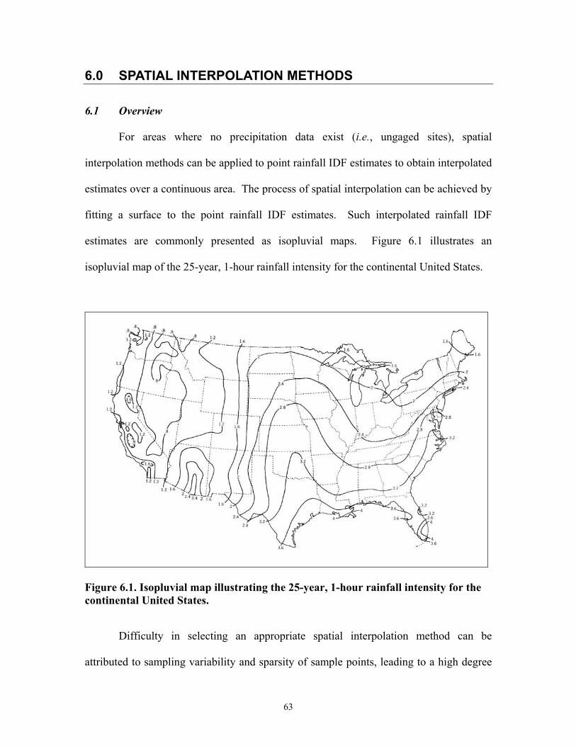
63

6.0 SPATIAL INTERPOLATION METHODS

6.1 Overview

For areas where no precipitation data exist (i.e., ungaged sites), spatial

interpolation methods can be applied to point rainfall IDF estimates to obtain interpolated

estimates over a continuous area. The process of spatial interpolation can be achieved by

fitting a surface to the point rainfall IDF estimates. Such interpolated rainfall IDF

estimates are commonly presented as isopluvial maps. Figure 6.1 illustrates an

isopluvial map of the 25-year, 1-hour rainfall intensity for the continental United States.

Figure 6.1. Isopluvial map illustrating the 25-year, 1-hour rainfall intensity for the continental United States.

Difficulty in selecting an appropriate spatial interpolation method can be

attributed to sampling variability and sparsity of sample points, leading to a high degree

64

of uncertainty in frequency analysis estimates. To assist in accurately interpolating over

a continuous area, regional information, such as distance from lake, elevation, or mean

annual precipitation, may be used to increase confidence in the interpolated estimates.

As described in previous chapters, the regional frequency analysis algorithm

applied in this study (Hosking and Wallis 1997) involves the identification of

homogeneous regions, where clustering may be based on site characteristics such as

geographical location, elevation, and other physical properties. After identification of

homogeneous regions, a three-parameter distribution is selected using a goodness-of-fit

test, and this distribution is then fitted to the data series to yield robust frequency-specific

quantile estimates for each region. Two of the distribution parameters (e.g., the standard

deviation and skew) are based on regional data and are assumed constant throughout the

region, while the third distibution parameter (e.g., the mean) is site-specific and subject to

sampling variability, therefore requiring spatial interpolation in order to derive isopluvial

maps. Following spatial interpolation, the site-specific distribution parameter is

multiplied by the frequency-specific quantile estimates for each region, resulting in

regional IDF estimates.

This chapter focuses on the evaluation and selection of appropriate spatial

interpolation techniques for generating isopluvial maps and determining rainfall IDF

estimates at ungaged sites. Techniques described in some of the early documentation of

rainfall IDF studies are investigated, as are more recently developed interpolation

methods. In addition, this chapter outlines the ordinary kriging algorithm chosen to

derive the new MDOT rainfall IDF estimates.

65

6.2 Previous Rainfall Frequency Studies

Early frequency analysis studies ignored the spatial distribution of rainfall by

assuming the areas of interest were small enough that point representations were

sufficiently representative of the regional variation in rainfall IDF estimates (Maidment

1993). As understanding of orographic effects improved, this assumption was no longer

acceptable in frequency analysis studies.

With increasing availability of rainfall data and the advent of digital computers,

spatial interpolation methods became useful tools for modeling regional variation in IDF

estimates. In 1961, the National Weather Service (NWS, then the U.S. Weather Bureau)

published Technical Paper 40 (Hershfield 1961) illustrating the development of forty-

nine isopluvial maps for the continental U.S. for the 1- to 100-year recurrence intervals

and 30-minute to 24-hour durations. Mathematical relationships consisting of ratio

constants, frequency and duration variables were derived allowing for the computation of

intensities for selected recurrence intervals and durations. By smoothing the data, the 2-

year, 1-hour and 24-hour isopluvial patterns were delineated. The smoothing process

consisted of drawing isolines between point values so that the standard deviation of the

estimates was approximately equal in respect to sampling and other errors in the data and

methods of analysis. To mask out local variation inherent in station-to-station estimates,

100-year to 2-year ratios for the 1- and 24-hour durations were plotted on a 3500-point

grid and used to construct the 100-year, 1-hour and 24-hour maps. The remaining forty-

five isopluvial maps were constructed by utilizing a computer program to plot a 3500-

point grid for each duration-recurrence interval combination.

66

Out of growing environmental awareness during the 1970s, there came about an

increase in demand for hydrologic planning and design for small drainage areas having

very short times of concentration. In response to this demand, the National Oceanic and

Atmospheric Administration (NOAA) was charged with updating Hershfield’s (1961) 5-

to 60-minute rainfall IDF estimates. Since it was found that orographic effects had a

greater significant influence in the eleven westernmost states of the continental U.S.,

separate studies were performed for the eastern and western states. These were published

as NOAA Atlas II (Miller et al. 1973) and NOAA Atlas I (Fredrick et al. 1977),

respectively.

In NOAA Atlas I (Fredrick et al. 1977), 6 isopluvial maps were developed for 2-

and 100-year recurrence intervals at 5-, 15-, and 60-minute durations for thirty-seven

states from North Dakota to Texas and eastward. In addition, mathematical relationships

for both recurrence interval and duration were derived to interpolate values for recurrence

intervals between 2 and 100 years. Fredrick et al. (1977) elected to use an approach

similar to Hershfield (1961) to develop ratio constants, however, they observed the ratios

varied with both geography and frequency. To minimize the variation in the ratios,

Fredrick et al. (1977) constructed six isopluvial maps and derived specific ratios for

intermediate recurrence intervals and durations between the constructed maps. The 2-

year, 60-minute isopluvial patterns were first constructed using a computerized space-

averaging (or smoothing) technique and then used for guidance in the directional

placement of isopluvial patterns for the remaining five maps. The space-averaging

technique divided the study area into 0.5° latitude x 0.5° longitude rectangular grids and

performed the following steps: 1) computed grid point averages using distance weighted

67

average of the stations’ values within latitude-longitude grids; 2) applied a double linear

interpolation function to estimate new station values and computed the difference in

original station values and interpolated values; and 3) adjusted grid point estimates

computed in step 1 by the average of the differences computed in step 2 and weighted by

the distance function. The analyst repeated steps 2 and 3 until a desired degree of

smoothing was achieved.

As understanding of hydrometeorological processes improved and more

precipitation data became available through more extensive gage networks and longer

gage records, it was determined that the earlier studies (Hershfield 1961; Miller et al.

1973; and Fredrick 1977) no longer presented the spatial resolution needed for certain

areas of the country. As a result, several state highway departments and water resource

agencies conducted independent frequency analysis studies to estimate local rainfall

variations more accurately.

In 1986, Dunn (1986) constructed five rainfall IDF curves illustrating 2- to 100-

year recurrence intervals and 5-minute to 24-hour durations for the Pennsylvania

Department of Transportation. Five “regions of similar rainfall intensities” for

Pennsylvania were delineated using four storm distributions, i.e., 2- and 100-year

recurrence intervals of 1- and 24-hour durations. The selection of the four storm

distributions was based on their wide variation in both recurrence interval and duration,

which enveloped the required recurrence intervals and durations for the study. Individual

rainfall intensities for the four storms were constructed. Based on the maximum and

minimum records in the four storm distributions combined, a classification scheme was

developed which divided intensities into five percentiles. After plotting the percent

68

magnitudes for each storm distribution, the four maps were overlaid and boundaries of

similar rainfall intensities were drawn. Orographic features and “peculiar histories” (such

as floods affecting Johnstown, PA) were considered in the final location of the five

regions.

By the late 1980s, the State of Illinois was motivated to revise IDF estimates due

to increased flooding in northern Illinois and a study showing apparent climatic trends

influencing frequency distributions of heavy rainstorms in Illinois from 1901-1980

(Angel and Huff 1997). In addition, Illinois’ IDF estimates had not been updated since

Hershfield’s (1961) work (Huff and Angel 1989). In 1989, the Illinois State Water

Survey Division published Bulletin 70 (Huff and Angel 1989), which updated rainfall

IDF estimates by dividing the state into ten “approximately homogeneous” climatic

sections based on assessment of gage data with consideration of meteorological and

climatological information. For each climatic division, Huff and Angel (1989) presented

the updated estimates in tabular and graphical (i.e., IDF curves) forms. In addition, forty-

eight isopluvial maps were developed for the 2- to 100-year recurrence intervals and 1- to

72-hour durations. Documentation on the development of the isopluvial maps provided

little information on the methodology used except that a combination of statistical

techniques, guided by available meteorological and climatological knowledge, was used.

In 1992, the Illinois State Water Survey Division published Bulletin 71 (Huff and Angel

1992) which updated rainfall IDF estimates for nine Midwest states (i.e., Illinois, Indiana,

Iowa, Kentucky, Michigan, Minnesota, Missouri, Ohio, and Wisconsin) using similar

procedures used in the Huff and Angel (1989) study.

69

In 1990, the Michigan Department of Natural Resources revised the rainfall IDF

estimates for the state of Michigan and presented the estimates as six isopluvial maps for

2- to 100-year recurrence intervals at the 24-hour duration (Sorrel and Hamilton 1990).

Very little documentation was provided on the methods used to construct the isopluvial

maps, except that a commercial plotting package was used to plot and contour rainfall

intensities, and minor irregularities were hand-adjusted.

Current MDOT rainfall IDF estimates are a compilation of results from three

rainfall frequency studies (U.S. Weather Bureau 1955; Hershfield 1961; Sorrell and

Hamilton 1990) (Michigan Department of Transportation 1996). As part of the Michigan

Road Design Manual, the state of Michigan was divided into four-rainfall frequency

zones (Michigan Department of Transportation 1996). For each zone, rainfall IDF

estimates are presented in tabular form for the 10- and 50-year recurrence intervals and

10- to 240-minute durations. No documentation was found on the methods used in

delineating the four frequency zones or compiling the IDF estimates.

Throughout the literature on frequency analysis studies, several interpolation

techniques have been employed to generate isopluvial maps from point IDF estimates.

Additionally, every study has incorporated some degree of smoothing to address

sampling variability (estimation error). However, these interpolation and smoothing

techniques have been highly subjective, requiring interaction with the analyst and relying

on expert knowledge and judgement. Subjective approaches make peer review difficult

and acceptance of the final results may be heavily based on the professional reputation of

the analyst. Objective mapping techniques, on the other hand, are reproducible and more

amenable to peer review.

70

6.3 Assessment of Spatial Interpolation Algorithms

A goal of this study is to use the most objective techniques available for spatial

interpolation of site-specific parameters in a regional analysis, while recognizing that

some engineering judgement will still be required. This section assesses the

appropriateness in spatially interpolating point IDF estimates of several spatial

interpolation algorithms. Although there are many spatial interpolation algorithms

available (Lancaster and Salkauskas 1986; Watson 1992), the review will be limited to

commonly used spatial interpolation methods, such as those available in a commercial

geostatistical software package or GIS. Specifically, the assessment will focus on the

strengths and weaknesses of the trend surface analysis, thin-plate splines, inverse distance

weighting, and kriging (ordinary, universal, and co-kriging) algorithms in developing

isopluvial maps.

6.3.1 Trend Surface Analysis

The trend surface analysis algorithm simply uses multiple regression (i.e., least

squares) to fit a polynomial surface to the entire set of observations. Since final

interpolated surfaces represent the broad regional trend in the variation implied by the

data, and seldom pass exactly through the original data points, the algorithm is typically

referred to as an inexact interpolator Figure 6.2 illustrates an example of a trend surface

of preliminary 2-year, 1-hour rainfall intensity estimates for Michigan in the y-z plane.

Comparing the point rainfall intensity estimates with the fitted curve illustrates the high

spatial variability and the degree of smoothing that is incorporated into the final

interpolated surface.

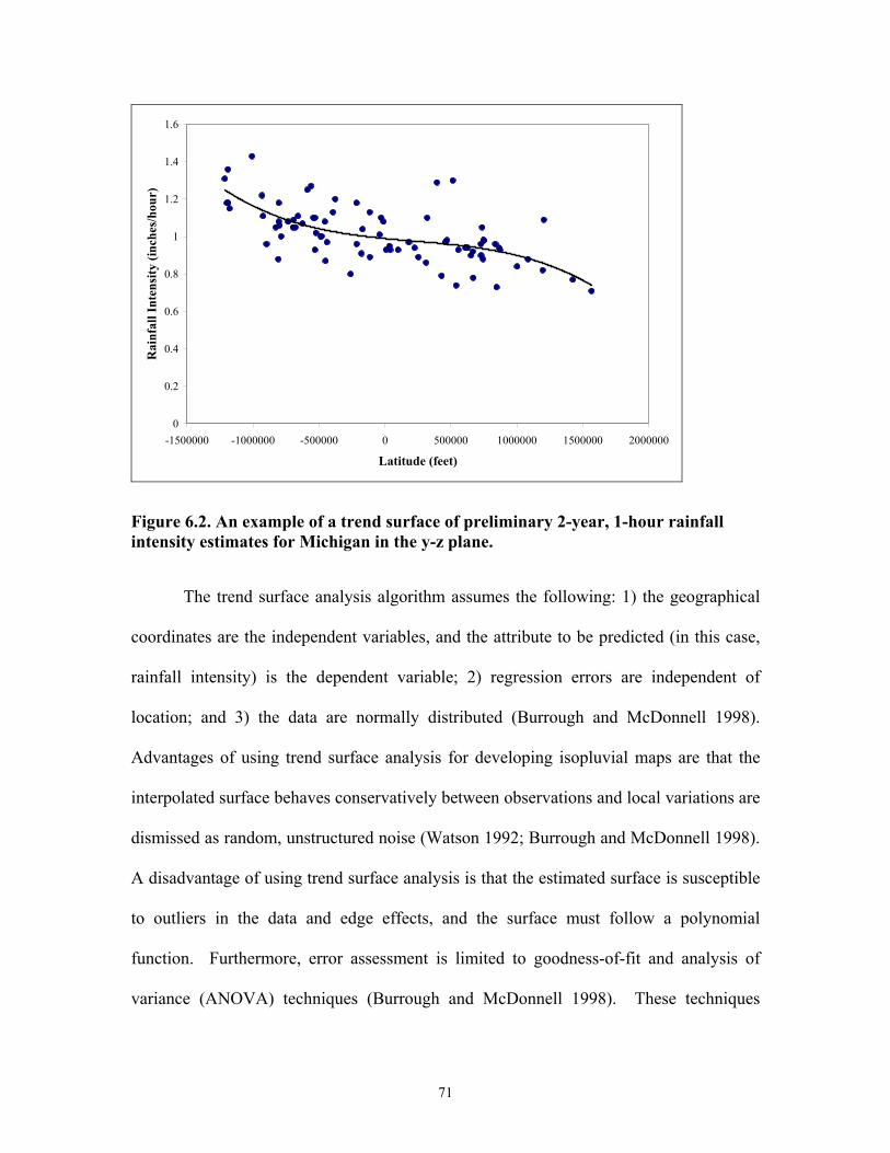
71

0

0.2

0.4

0.6

0.8

1

1.2

1.4

1.6

-1500000 -1000000 -500000 0 500000 1000000 1500000 2000000

Latitude (feet)

Rai

nfal

l Int

ensi

ty (i

nche

s/ho

ur)

Figure 6.2. An example of a trend surface of preliminary 2-year, 1-hour rainfall intensity estimates for Michigan in the y-z plane.

The trend surface analysis algorithm assumes the following: 1) the geographical

coordinates are the independent variables, and the attribute to be predicted (in this case,

rainfall intensity) is the dependent variable; 2) regression errors are independent of

location; and 3) the data are normally distributed (Burrough and McDonnell 1998).

Advantages of using trend surface analysis for developing isopluvial maps are that the

interpolated surface behaves conservatively between observations and local variations are

dismissed as random, unstructured noise (Watson 1992; Burrough and McDonnell 1998).

A disadvantage of using trend surface analysis is that the estimated surface is susceptible

to outliers in the data and edge effects, and the surface must follow a polynomial

function. Furthermore, error assessment is limited to goodness-of-fit and analysis of

variance (ANOVA) techniques (Burrough and McDonnell 1998). These techniques

72

usually assume that rainfall IDF estimates are normally distributed, which is typically not

the case.

6.3.2 Thin-plate Splines

Thin-plate splines also use multiple regression to fit a polynomial surface to a set

of observations. However, the algorithm performs piece-wise multiple regression on

subsets of observations that are within a predefined neighborhood, which allows local

variation in the observations to be retained in the final interpolated surface. Figure 6.3

illustrates an one-dimensional view of piece-wise polynomial regression using thin-plate

splines on a sub-set of 2-year, 1-hour rainfall intensity estimates. Through piece-wise

polynomial regression, all of the spatial variability is incorporated into the final

interpolated surface.

73

0.6

0.7

0.8

0.9

1

1.1

1.2

0 500 1000 1500 2000 2500 3000 3500

Distance (feet)

Rai

nfal

l Int

ensi

ty (i

nche

s/ho

ur)

Figure 6.3. Cross-section of a piece-wise multiple regression using thin-plate splines on a subset of 2-year, 1-hour rainfall intensity estimates defined by a pre-defined neighborhood.

Splines follow the general notion that interpolated values are similar to the nearest

known observation values. The algorithm imposes the following two conditions: 1) the

surface must pass exactly through observation points, and 2) the surface must have

minimum curvature, i.e., the least possible change in slope, at each observation point.

The advantage of using thin-plate splines with respect to rainfall IDF estimates is that

only observations within a predefined vicinity influence interpolated values. The

disadvantages of thin-plate splines are that there is no method for selecting an appropriate

neighborhood radius size, and there is no direct method for assessing the error in

interpolated values. Also, interpolated surfaces may contain unrealistic highs and lows as

a result of exact interpolation (Burrough and McDonnell 1998), as apparent in Figure 6.3

at a distance of approximately 2900 feet.

74

6.3.3 Inverse Distance Weighting

Similar to thin-plate splines, inverse distance weighting follows the principle that

nearby observation points are more influential than distant observations. The inverse

distance weighting algorithm involves the following steps: 1) select the nearest

observation points within a predefined neighborhood; 2) assign a weight to each

observation based on its distance from the interpolation point; 3) sum the weighted

observations to determine an average. Weights are assigned for each observation point

within the search neighborhood using Equation 6.1 (Watson 1992):

∑=

−

−

= N

j

pi

pi

i

d

dw

1

(6.1)

where iw is the weight assign to the ith observation point, id is the distance to the ith

observation point from the interpolation point, and p is an arbitrary power of distance,

which influences how the interpolated surface behaves between points (Watson 1992).

Due to the mathematical nature of inverse distance weighting, the algorithm is an exact

interpolator, as shown in Equation 6.1 (at an observation point location, the weight tends

to infinity). The advantages of using inverse distance weighting for isopluvial maps are

that the interpolated surface is confined within the range of the point values, and only

observations within a predefined vicinity influence the interpolated estimates.

Disadvantages of the algorithm are that there are no methods of testing the quality of

predictions, the final interpolated surface is strongly dependent on the size of the

neighborhood radius and dominated by local variation, and the surface slope may be

discontinuous at observation points as a result of exact interpolation.

75

6.3.4 Kriging

Kriging is the geostatistical method of interpolation that provides the best, i.e.,

minimum variance, unbiased linear estimates of the value of a parameter at unmeasured

locations from a set of observations. Similar to inverse distance weighting, the kriging

algorithm models spatial variation by assigning weights to the observations within a

predefined search neighborhood, as shown in Equation 6.2 (Burrough and McDonnell

1998).

∑=

⋅=n

iii xzxz

10 )()(ˆ λ (6.2)

where ix are measured (observed) values; iλ are assigned weights, where ∑=

=n

ii

11λ so

that the estimate is unbiased; and )(ˆ 0xz is the value to be estimated at location 0x .

However, unlike the previously discussed algorithms, kriging also provides a theoretical

basis for determining the most appropriate weights and size of the search neighborhood.

Kriging optimizes spatial interpolation based on the assumption that spatial variation

consists of three major components: 1) a structural component, having a constant mean or

trend; 2) a random, but spatially correlated component; and 3) a spatially uncorrelated

component (random noise or residual error) (Burrough and McDonnell 1998). This

treatment of the variation is known as the regionalized variable theory, which is based on

the intrinsic hypothesis that assumes once structural effects have been accounted for, the

remaining variation is homogeneous, i.e., differences between sites are only a function of

distance (Armstrong 1998). Although there are several variations of kriging, only

ordinary kriging, universal kriging, and co-kriging will be assessed for use in this study to

develop isopluvial maps.

76

Ordinary kriging provides a means of interactively investigating the spatial

variation of the data, which allows for the selection of the best estimation method prior to

generating the final interpolated surface. This process involves computing the

experimental semivariogram and fitting to it a suitable semivariogram model. Common

semivariogram models are the spherical, circular, exponential, Gaussian, and linear

models (Armstrong 1998; Watson 1992). Estimating parameters of the semivariogram

model (lag distance, nugget, range, and sill) acts as a surrogate for identifying appropriate

interpolation control parameters, such as the size of the search neighborhood and the

necessary weighting. Figure 6.4 illustrates a theoretical semivariogram model fitted to an

experimental semivariogram with several model parameters labeled.

Figure 6.4. An example of a semivariogram model fitted to the experimental semivariogram, with identification of the nugget, range, and sill.

The presence of a nugget signifies variation due to measurement error or

uncorrelated, unstructured noise. The range represents the distance beyond which

77

observations have no influence on the interpolated estimate. For most semivariogram

models, the range is identified as the distance at which the semivariance levels off (at the

value of the sill). Just as bin size is used in constructing histograms, the lag distance is

the separation distance between points for which the squared difference (i.e., the

covariance) in the attribute being interpolated is averaged and plotted as part of the

experimental semivariogram.

Advantages of using ordinary kriging for mapping rainfall IDF estimates are that

the use of a semivariogram model assists in the selection of appropriate interpolation

control parameters, and the algorithm provides a direct estimate of the quality of the

interpolated surface in terms of the estimation variance. Disadvantages of ordinary

kriging are that the selection of the appropriate semivariogram model and lag distance

introduces some degree of subjectivity and requires knowledge of geostatistical theory.

Universal kriging combines the theories of trend surface analysis and ordinary

kriging and is used when a known trend exists in the data (Burrough and McDonnell

1998). Trend surface analysis is first performed on the data to remove the existing trend.

Ordinary kriging is then performed on the residuals of the trend surface. As a final step,

the trend is added back into the ordinary kriging result performed on the residuals. An

advantage of using universal kriging for mapping rainfall IDF estimates is that it provides

a direct estimate of the quality of the interpolated surface in terms of the estimation

variance. Disadvantages of using universal kriging are similar to those already discussed

for trend surface analysis and ordinary kriging.

Both ordinary and universal kriging deal with only one regionalized variable. In

several instances, incorporating additional correlated variables may provide improvement

78

in interpolation. Co-kriging is a multivariate geostatistical technique that considers the

spatial variation of additional variables that are correlated with the variable of interest

(Burrough and McDonnell 1998). Similar to ordinary kriging, co-kriging provides an

interactive process of selecting the best estimation method prior to generating the final

interpolated surface. However, the interactive process in co-kriging involves computing

an experimental semivariogram for each variable, overlaying the experimental

semivariograms, and fitting a suitable theoretical semivariogram model to the collection.

The result is the development of a theoretical covariogram. The covariogram has the

same functions as the semivariogram of ordinary kriging.

Co-kriging is advantageous in situations where the variable of interest 1) is a

linear combination of regionalized variables; 2) is poorly sampled but correlates highly

with one or more variables that are much better sampled; or 3) exhibits low spatial

autocorrelation, but correlates highly with one or more variables that exhibit relatively

high continuity. While co-kriging should always provide results at least as good as those

from ordinary kriging, in some situations, co-kriging may not provide significant

improvement considering the additional effort required by the analyst. Therefore, Hohn

(1988) suggested first obtaining kriged and cokriged results from a typical sample

configuration to ensure significant improvement in the estimates is possible.

6.4 Algorithm Selection

The accuracy of an interpolated surface depends on several factors: 1) the number

of observation points and the quality of the data at each point, 2) the orientation and

spacing of the observations, 3) the distance between observations to be interpolated, and

4) the spatial continuity of the variable under consideration (Armstrong 1998).

79

Developing accurate isopluvial maps can be a challenge because there are usually a

limited number of station gages that have record lengths sufficient for deriving accurate

point IDF estimates. Nonetheless, an ideal method for spatial interpolation of these point

estimates would do the following: 1) fit a continuous, gradually varying surface to the

point estimates, 2) recognize the estimation error in the point values, 3) provide a direct

means of assessing the quality of the interpolated surface, and 4) minimize subjectivity of

expert judgement.

Table 6.1 compares six spatial interpolation algorithms available in a commercial

geostatistical software package, based on the four criteria defining an ideal interpolation

algorithm for site-specific parameters. Although kriging, in general, is considered an

exact interpolator, local variation may be smoothed in order to model only the broad

spatial variation by selecting a nugget size greater than zero during the development of

the semivariogram and covariogram. Varying the grid size for the final interpolated

surface may also incorporate some degree of smoothing of the local spatial variation.

Therefore, each of the three kriging algorithms, as well as trend surface analysis, is

capable of recognizing the estimation error, i.e. uncertainty, in the site-specific parameter.

However, only the three kriging algorithms provide a direct means of assessing the

quality of the interpolated surface by generating the estimation variance at each

interpolated point. In addition, each of the kriging algorithms minimizes subjectivity of

expert judgement by providing objective means for selecting appropriate control

parameters used during the interpolation process through the semivariogram and/or

covariogram. Therefore, ordinary kriging, universal, and co-kriging appear to be the

most appropriate of the methods previously discussed. All three kriging algorithms are

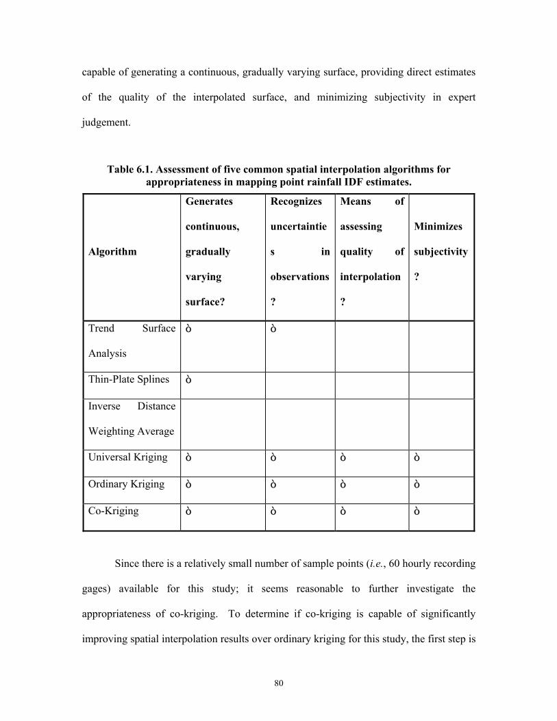
80

capable of generating a continuous, gradually varying surface, providing direct estimates

of the quality of the interpolated surface, and minimizing subjectivity in expert

judgement.

Table 6.1. Assessment of five common spatial interpolation algorithms for appropriateness in mapping point rainfall IDF estimates.

Algorithm

Generates

continuous,

gradually

varying

surface?

Recognizes

uncertaintie

s in

observations

?

Means of

assessing

quality of

interpolation

?

Minimizes

subjectivity

?

Trend Surface

Analysis

ò ò

Thin-Plate Splines ò

Inverse Distance

Weighting Average

Universal Kriging ò ò ò ò

Ordinary Kriging ò ò ò ò

Co-Kriging ò ò ò ò

Since there is a relatively small number of sample points (i.e., 60 hourly recording

gages) available for this study; it seems reasonable to further investigate the

appropriateness of co-kriging. To determine if co-kriging is capable of significantly

improving spatial interpolation results over ordinary kriging for this study, the first step is

81

to identify additional regionalized variables that are well correlated with rainfall IDF

estimates. Distance from the closest Great Lake, elevation, and mean annual

precipitation are identified as regionalized variables that one may expect to be well

correlated with point rainfall IDF estimates.

Figure 6.5 illustrates a scatter plot of 2-year, 1-hour rainfall intensities versus

distance from the closest Great Lake for 60 selected hourly recording stations in

Michigan. The scatter plot suggests that distance from a Great Lake may be slightly

correlated with the 2-year, 1-hour rainfall intensity estimates. A standard statistical t-test

(DeGroot 1986) was performed to determine the significance of the slope obtained from

simple linear regression. Results from the t-test showed that, at the 0.001 significance

level, the null hypothesis (i.e., H0: slope = 0) should be rejected. However, such a high

significance in the slope may actually be biased since there are relatively few rainfall

gages 50 miles or more from a Great Lake. In addition, the low coefficient of

determination (i.e., R2 = 0.1265) indicates rainfall IDF estimates and distance from the

closest Great Lake are not well correlated.

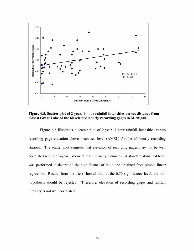
82

y = 0.0018x + 0.9515R2 = 0.1265

0.70

0.80

0.90

1.00

1.10

1.20

1.30

0 10 20 30 40 50 60 70 80

Distance from a Great Lake (miles)

Rai

nfal

l Int

ensi

ty (i

nche

s/ho

ur)

Figure 6.5. Scatter plot of 2-year, 1-hour rainfall intensities versus distance from closest Great Lake of the 60 selected hourly recording gages in Michigan.

Figure 6.6 illustrates a scatter plot of 2-year, 1-hour rainfall intensities versus

recording gage elevation above mean sea level (AMSL) for the 60 hourly recording

stations. The scatter plot suggests that elevation of recording gages may not be well

correlated with the 2-year, 1-hour rainfall intensity estimates. A standard statistical t-test

was performed to determine the significance of the slope obtained from simple linear

regression. Results from the t-test showed that, at the 0.50 significance level, the null

hypothesis should be rejected. Therefore, elevation of recording gages and rainfall

intensity is not well correlated.

83

y = -3E-06x + 0.9965R2 = 4E-05

0.70

0.80

0.90

1.00

1.10

1.20

1.30

500 600 700 800 900 1000 1100 1200 1300 1400 1500 1600

Elevation (feet AMSL)

Rai

nfal

l Int

ensi

ty (i

nche

s/ho

ur)

Figure 6.6. Scatter plot of 2-year, 1-hour rainfall intensities versus elevation (AMSL) of recording gages of the 60 selected hourly recording gages in Michigan.

Finally, Figure 6.7 illustrates a scatter plot of 2-year, 1-hour rainfall intensities

versus mean annual precipitation for the 60 selected hourly recording stations. The

scatter plot suggests that mean annual precipitation may be slightly correlated with the 2-

year, 1-hour rainfall intensity estimates. A standard statistical t-test was performed to

determine the significance of the slope obtained from simple linear regression. Results

from the t-test showed that, at the 0.05 significance level, the null hypothesis should be

rejected. However, as indicated by the low coefficient of determination (i.e., R2 =

0.0674), rainfall IDF estimates and mean annual precipitation are not well correlated.

Thus, co-kriging would not be expected to offer a significant improvement over ordinary

kriging or universal kriging.

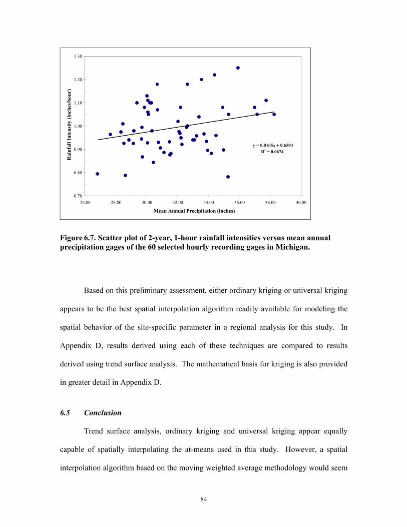
84

y = 0.0105x + 0.6594R2 = 0.0674

0.70

0.80

0.90

1.00

1.10

1.20

1.30

26.00 28.00 30.00 32.00 34.00 36.00 38.00 40.00

Mean Annual Precipitation (inches)

Rai

nfal

l Int

ensi

ty (i

nche

s/ho

ur)

Figure 6.7. Scatter plot of 2-year, 1-hour rainfall intensities versus mean annual precipitation gages of the 60 selected hourly recording gages in Michigan.

Based on this preliminary assessment, either ordinary kriging or universal kriging

appears to be the best spatial interpolation algorithm readily available for modeling the

spatial behavior of the site-specific parameter in a regional analysis for this study. In

Appendix D, results derived using each of these techniques are compared to results

derived using trend surface analysis. The mathematical basis for kriging is also provided

in greater detail in Appendix D.

6.5 Conclusion

Trend surface analysis, ordinary kriging and universal kriging appear equally

capable of spatially interpolating the at-means used in this study. However, a spatial

interpolation algorithm based on the moving weighted average methodology would seem

85

most appropriate given the nature of rainfall IDF estimates. Since universal kriging was

not found to provide improved results over ordinary kriging, while introducing additional

complexity, ordinary kriging appears to be the most appropriate spatial interpolation

algorithm readily available for modeling the spatial variation in the at-site means for this

study. Since weighting is assigned to sampled observations on a moving neighborhood

basis, where the nearest observations are given greater influence at locations being

estimated, the interpolated estimates are more similar to neighboring sample observations

than to distant observations. Furthermore, through the selection of a semivariogram

model and estimation of its parameters, the analyst can specify the size of the

neighborhood.

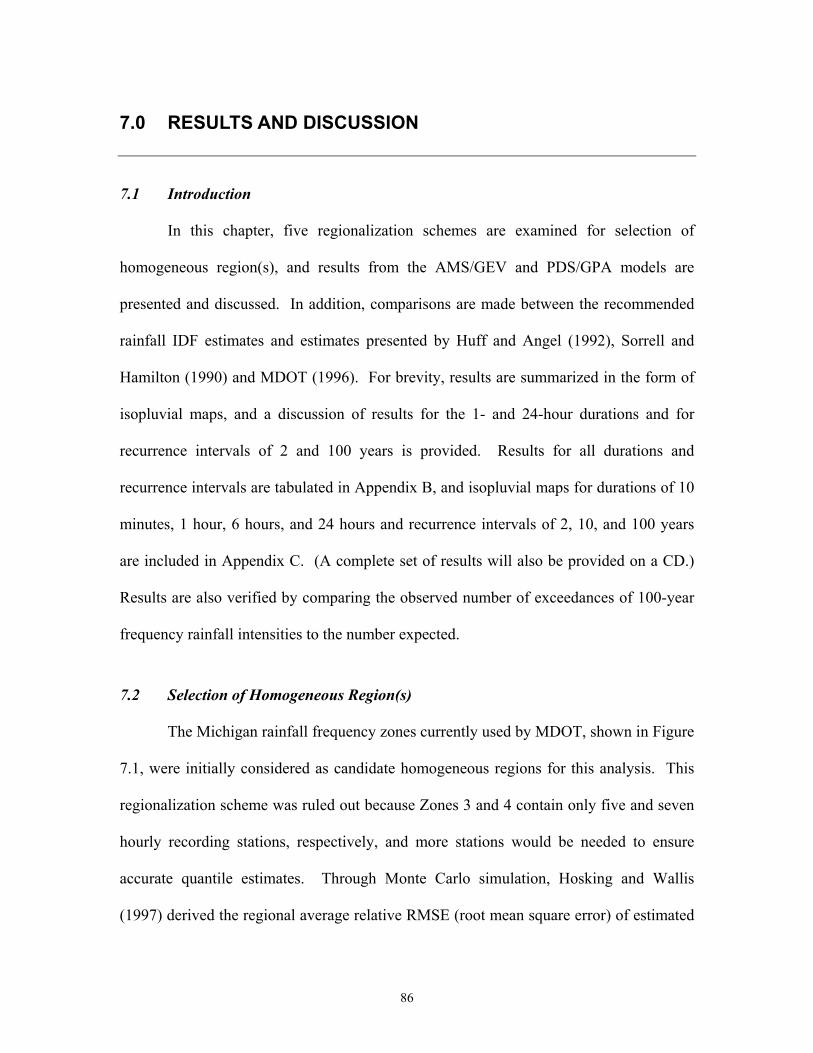
86

7.0 RESULTS AND DISCUSSION

7.1 Introduction

In this chapter, five regionalization schemes are examined for selection of

homogeneous region(s), and results from the AMS/GEV and PDS/GPA models are

presented and discussed. In addition, comparisons are made between the recommended

rainfall IDF estimates and estimates presented by Huff and Angel (1992), Sorrell and

Hamilton (1990) and MDOT (1996). For brevity, results are summarized in the form of

isopluvial maps, and a discussion of results for the 1- and 24-hour durations and for

recurrence intervals of 2 and 100 years is provided. Results for all durations and

recurrence intervals are tabulated in Appendix B, and isopluvial maps for durations of 10

minutes, 1 hour, 6 hours, and 24 hours and recurrence intervals of 2, 10, and 100 years

are included in Appendix C. (A complete set of results will also be provided on a CD.)

Results are also verified by comparing the observed number of exceedances of 100-year

frequency rainfall intensities to the number expected.

7.2 Selection of Homogeneous Region(s)

The Michigan rainfall frequency zones currently used by MDOT, shown in Figure

7.1, were initially considered as candidate homogeneous regions for this analysis. This

regionalization scheme was ruled out because Zones 3 and 4 contain only five and seven

hourly recording stations, respectively, and more stations would be needed to ensure

accurate quantile estimates. Through Monte Carlo simulation, Hosking and Wallis

(1997) derived the regional average relative RMSE (root mean square error) of estimated

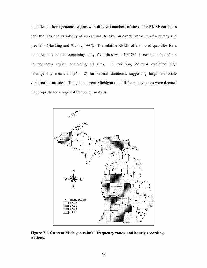
87

quantiles for homogeneous regions with different numbers of sites. The RMSE combines

both the bias and variability of an estimate to give an overall measure of accuracy and

precision (Hosking and Wallis, 1997). The relative RMSE of estimated quantiles for a

homogeneous region containing only five sites was 10-12% larger than that for a

homogeneous region containing 20 sites. In addition, Zone 4 exhibited high

heterogeneity measures (H > 2) for several durations, suggesting large site-to-site

variation in statistics. Thus, the current Michigan rainfall frequency zones were deemed

inappropriate for a regional frequency analysis.

Figure 7.1. Current Michigan rainfall frequency zones, and hourly recording stations.

88

To identify homogeneous regions, cluster analysis based on site characteristics is

recommended (Hosking and Wallis, 1997). In appraising geostatistical methods for

estimating rainfall at ungaged sites, evaluated the correlation between rainfall intensity

and site characteristics that are commonly associated with heavy rainfall. Little

correlation was found between rainfall intensity and distance from the closest Great Lake,

elevation, and mean annual precipitation. In other words, sampling variability obscures

whatever correlation exists. In light of these findings, and the fact that the homogeneity

criteria were satisfied with all sites lumped into one region, it was deemed that the State

potentially could be treated as one homogeneous region.

To examine the possible adverse effects of treating the State as one region, three

other regionalization schemes were evaluated and the resulting quantile estimates

compared. Cluster analysis procedures were used to aid in identifying two or three

smaller homogeneous regions within the State. Clustering was based on the following

site characteristics: latitude, longitude, elevation, and mean annual precipitation (MAP).

In the clustering procedure, MAP was given twice as much weight as the other site

characteristics. The resulting clusters of hourly recording stations for the two and three

regions are shown in Figures 7.2 and 7.3, respectively. It should be noted that the daily

station clusters are identical to those in Figures 7.2 and 7.3, but with greater station

density.

89

Figure 7.2. Two clusters (or regions) of hourly recording stations formed using cluster analysis procedures with mean annual precipitation given double weight.

90

Figure 7.3. Three clusters (or regions) of hourly recording stations formed using cluster analysis procedures with mean annual precipitation given double weight.

In an effort to maximize differences in quantile estimates between two

homogeneous regions within the State, a third regional scenario was evaluated.

Recognizing that moist air masses from the Gulf of Mexico are a major driving force

behind rainfall intensity for the Midwestern United States, the State was divided into a

north region and a south region using county boundaries as a guide, as shown in Figure

7.4.

91

Figure 7.4. North-South regions and hourly recording gages. Regions are formed subjectively in an effort to maximize differences in regional quantile estimates.

In evaluating these regional scenarios, little variation was found between at-site

statistics and the regional average statistics. As a result, heterogeneity measures were not

a reliable method for determining regions (i.e., no matter how the regions were formed,

the homogeneity conditions were always satisfied). Table 7.1 shows an example of this

for 6-hour AMS data. For the regionalization schemes considered, the homogeneity

conditions are satisfied for each cluster.

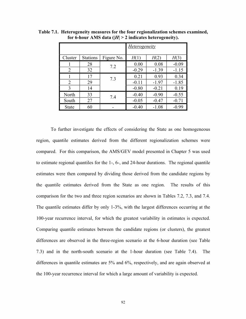
92

Table 7.1. Heterogeneity measures for the four regionalization schemes examined, for 6-hour AMS data (|H| > 2 indicates heterogeneity).

Heterogeneity

Cluster Stations Figure No. H(1) H(2) H(3) 1 28 0.00 0.08 -0.09 2 32

7.2 -0.29 -1.39 -1.15

1 17 0.21 0.93 0.34 2 29 -0.11 -1.97 -1.85 3 14

7.3

-0.80 -0.21 0.19 North 33 -0.40 -0.90 -0.55 South 27

7.4 -0.05 -0.47 -0.71

State 60 - -0.40 -1.08 -0.99

To further investigate the effects of considering the State as one homogeneous

region, quantile estimates derived from the different regionalization schemes were

compared. For this comparison, the AMS/GEV model presented in Chapter 5 was used

to estimate regional quantiles for the 1-, 6-, and 24-hour durations. The regional quantile

estimates were then compared by dividing those derived from the candidate regions by

the quantile estimates derived from the State as one region. The results of this

comparison for the two and three region scenarios are shown in Tables 7.2, 7.3, and 7.4.

The quantile estimates differ by only 1-3%, with the largest differences occurring at the

100-year recurrence interval, for which the greatest variability in estimates is expected.

Comparing quantile estimates between the candidate regions (or clusters), the greatest

differences are observed in the three-region scenario at the 6-hour duration (see Table

7.3) and in the north-south scenario at the 1-hour duration (see Table 7.4). The

differences in quantile estimates are 5% and 6%, respectively, and are again observed at

the 100-year recurrence interval for which a large amount of variability is expected.

93

Table 7.2. Ratios of the candidate regional quantile estimates to those derived from the State as one region, for the two clusters shown in Figure 7.2.

Cluster Stations Duration 2-year 5-year 10-year 25-year 50-year 100-year1 28 1.00 1.00 1.00 0.99 0.99 0.992 32 1.00 1.00 1.00 1.01 1.01 1.011 28 1.00 1.00 1.00 1.01 1.01 1.012 32 1.00 1.00 1.00 0.99 0.99 0.991 74 1.00 1.00 1.00 1.00 1.00 1.002 78 1.00 1.00 1.00 1.00 1.00 1.00

Regional Quantile Estimate Ratios for the T -year Event

1-hour

6-hour

24-hour

Table 7.3. Ratios of the candidate regional quantile estimates to those derived from the State as one region, for the three clusters shown in Figure 7.3.

Cluster Stations Duration 2-year 5-year 10-year 25-year 50-year 100-year1 17 1.00 0.99 0.99 0.99 0.99 0.992 29 1.00 1.00 1.00 1.00 1.00 1.003 14 1.00 1.01 1.02 1.02 1.02 1.021 17 0.99 1.00 1.01 1.01 1.02 1.032 29 1.00 1.00 0.99 0.99 0.99 0.983 14 1.00 1.00 1.00 1.00 1.00 1.001 61 1.00 1.00 1.00 1.00 1.00 1.002 77 1.00 1.00 1.00 1.00 1.00 1.003 14 1.00 1.01 1.01 1.00 1.00 0.99

Regional Quantile Estimate Ratios for the T -year Event

1-hour

6-hour

24-hour

Table 7.4. Ratios of the north-south regional quantile estimates to those derived from the State as one region, for the regions shown in Figure 7.4.

Cluster Stations Duration 2-year 5-year 10-year 25-year 50-year 100-yearNorth 33 0.99 1.00 1.01 1.02 1.02 1.03South 27 1.01 1.00 0.99 0.98 0.98 0.97North 33 1.00 1.00 0.99 0.99 0.99 0.99South 27 1.00 1.00 1.01 1.01 1.01 1.01North 74 1.01 1.00 1.00 0.99 0.98 0.98South 78 1.00 1.00 1.00 1.01 1.01 1.02

6-hour

24-hour

Regional Quantile Estimate Ratios for the T -year Event

1-hour

94

Because the noted differences were deemed to be insignificant for the purposes of

this study, the results were derived for the State as one region.

7.3 Comparison of Annual Maximum and Partial Duration Series Results

As described in Chapter 5, the annual maximum series (AMS) and partial

duration series (PDS) results were compiled using the index flood regional frequency

analysis procedure outlined by Hosking and Wallis (1997), with the State considered one

homogeneous region. Summaries of discordancy, heterogeneity and goodness-of-fit

measures for AMS and PDS data are given in Tables 7.5 and 7.6, respectively.

The discordancy measure was used for data verification and quality control.

Stations with a discordancy value of 3 or greater are considered discordant, while stations

with a value of 5 or greater are highly discordant. The threshold values of 3 and 5 are not

based on a rigorous test, but are considered reasonable levels to be expected within a

homogeneous region (Hosking and Wallis, 1997). Considering all seven durations for the

AMS data, a total of four stations were determined to be highly discordant (see Table

7.5), while in considering all eleven durations for the PDS data, six stations were found

highly discordant (see Table 7.6). In most cases, these high levels of discordancy were

attributed to a station observing a large outlier. It was deemed that these discordant

stations contained important data for estimating extreme rainfall intensities for Michigan.

Therefore, all stations were included in the analyses.

For the seven durations for the AMS data and the eleven durations for the PDS

data, heterogeneity measures generally indicate that it is suitable to consider the State as

one homogeneous region. Only for the 5-, 10-, 15-minute, and 1-hour PDS data was

there strong evidence of heterogeneity (|H(1)| > 2). Because the short duration values are

95

the most variable of the durations considered, and the other two heterogeneity

measures—H(2) and H(3)—indicate regional homogeneity, the high values were deemed

to be acceptable for the short durations.

Table 7.5. Summary of test statistics derived from annual maximum series data, considering the State as one region.

Duration Stations D i > 3 3<D i <5 D i >5 H (1) H (2) H (3) GLO GEV LN31-hour 60 3 1 2 0.31 0.5 1.20 2.56 -2.07 -2.772-hour 60 5 5 0 -0.39 0.04 0.07 3.23 -0.95 -1.983-hour 60 2 1 1 -0.69 -0.43 -0.31 2.87 -1.02 -2.206-hour 60 3 2 1 -0.40 -1.08 -0.99 1.68 -1.83 -3.1012-hour 60 4 4 0 -0.06 -1.93 -1.43 1.14 -2.33 -3.5618-hour 60 2 2 0 0.29 -2.07 -1.99 1.30 -2.24 -3.4524-hour 152 7 7 0 -0.64 -0.80 -0.43 1.83 -4.27 -6.80

Discordancy Heterogeneity Goodness-of-fit (Z- statistic)

Table 7.6. Summary of test statistics derived from partial duration series data, considering the State as one region.

Duration Stations D i > 3 3<D i <5 D i >5 H (1) H (2) H (3) GPA PE3 LN35 min 76 3 1 2 -4.14 -0.41 -0.19 -2.44 -1.73 4.1210 min 76 1 1 0 -2.17 -0.45 -0.05 -0.88 0.52 6.5615 min 76 2 2 0 -2.22 0.80 0.93 -0.07 0.94 7.1630 min 76 4 2 2 1.15 1.33 0.92 -0.29 0.34 6.571-hour 60 2 1 1 2.20 0.18 0.48 0.05 -1.76 4.632-hour 60 3 2 1 0.12 -0.47 -0.42 0.38 -2.21 4.263-hour 60 2 2 0 -1.00 -0.53 -0.43 0.40 -2.60 3.876-hour 60 2 2 0 -1.92 -0.07 -0.33 -0.77 -3.73 2.44

12-hour 60 3 3 0 -2.00 -0.98 -0.90 -0.68 -3.81 2.3718-hour 60 3 3 0 -1.28 -1.73 -1.74 -0.65 -3.54 2.6724-hour 152 5 5 0 0.48 0.34 0.58 -1.99 -7.55 4.44

Note:H (1) - Based on L -CV onlyH (2) - Based on L -CV and L -skewnessH (3) - Based on L -skewness and L -kurtosisGLO - Generalized Logistic distributionGEV - Generalized Extreme Value distributionLN3 - Lognormal distributionGPA - Generalized Pareto distributionPE3 - Pearson Type III distribution

Discordancy Heterogeneity Goodness-of-fit ( Z- statistic)

96

The goodness-of-fit measure Z was used to aid in identifying candidate

distributions that would yield robust quantile estimates for the State. This test measures

the distance between the regional average L-kurtosis and the theoretical L-kurtosis of the

candidate distributions. For the five distributions tested, the three that were closest to

meeting the Z criterion are shown in Tables 7.5 and 7.6. Those in bold have met the

criterion of |Z| < 1.64, which corresponds to the failure to reject the hypothesized

distribution at a confidence level of 90% (Hosking and Wallis, 1997).

For the AMS data (see Table 7.5), the Z-statistic is not a clear indicator of which

distribution provides the best fit to the data. The GEV distribution provides the best fit

for 3 durations, while the GLO distribution provides the best fit for the other 4 durations,

with both satisfying the Z criterion twice. However, a literature search did not find an

application of the GLO distribution to rainfall frequency analysis, while the GEV

distribution and its two-parameter variant, the Gumbel distribution, have found wide

application (e.g., Hershfield, 1961; Frederick, 1977; Sorrell and Hamilton, 1990;

Schaefer, 1990; and Loucks et al., 2000). Furthermore, the AMS/GEV model has a close

theoretical relationship with the PDS/GPA model, as discussed in Chapter 5. Thus, the

GEV distribution was selected.

In contrast, the GPA distribution clearly provides the best fit to the PDS data for

all 11 durations (see Table 7.6). Furthermore, the Z criterion is met for 9 of the durations.

Consequently, the GPA distribution was selected to derive rainfall IDF estimates from

the PDS data.

For the 24-hour duration, Tables 7.5 and 7.6 show that none of the candidate

distributions meet the Z criterion. Hosking and Wallis (1997) note that this sometimes

97

occurs when there are numerous sites in a region, or when the at-site record lengths are

large. The fact that there are 152 daily recording stations with an average record of 63

years (27 stations with over 100 years of record) incorporated in this study, which may

explain why none of the candidate distributions provide an acceptable fit.

The AMS/GEV and PDS/GPA distribution parameters and regional quantile

estimates (which are multiplied by the at-site means to determine IDF values) are shown

in Tables 7.7 and 7.8, respectively. The AMS/GEV quantiles for the 2-, 5- and 10-year

recurrence intervals have been converted to corresponding PDS values using the factors

discussed in Chapter 3. Because of the arbitrary beginning and ending of an hour or day,

quantile estimates from both models for the 1-, 2-, 3- and 24-hour durations have been

converted from clock-hour quantiles to actual (time-correct) quantiles (see Chapter 3).

Note that the PDS/GPA model regional quantile estimates are slightly larger than the

AMS/GEV quantiles regardless of duration and recurrence interval. This is because the

PDS/GPA quantiles are based on more frequent storm events (F = 1-1/λT) than are the

AMS/GEV quantiles (F = 1-1/T). Compensating for this mathematically, the PDS index

floods (at-site means) are lower than the corresponding means derived from the AMS

data.

For convenience, isopluvial maps were constructed to display and compare final

quantile estimates. For brevity, results are for the 1- and 24-hour durations and for

recurrence intervals of 2 and 100 years are discussed. Results for other selected durations

and recurrence intervals are provided in Appendix C, and a complete set of results is

available on the accompanying CD.

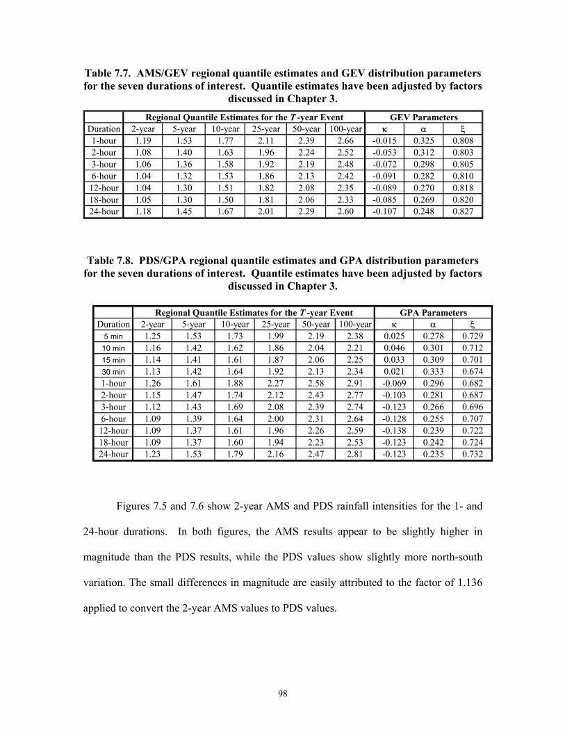
98

Table 7.7. AMS/GEV regional quantile estimates and GEV distribution parameters for the seven durations of interest. Quantile estimates have been adjusted by factors

discussed in Chapter 3.

Duration 2-year 5-year 10-year 25-year 50-year 100-year κ α ξ1-hour 1.19 1.53 1.77 2.11 2.39 2.66 -0.015 0.325 0.8082-hour 1.08 1.40 1.63 1.96 2.24 2.52 -0.053 0.312 0.8033-hour 1.06 1.36 1.58 1.92 2.19 2.48 -0.072 0.298 0.8056-hour 1.04 1.32 1.53 1.86 2.13 2.42 -0.091 0.282 0.810

12-hour 1.04 1.30 1.51 1.82 2.08 2.35 -0.089 0.270 0.81818-hour 1.05 1.30 1.50 1.81 2.06 2.33 -0.085 0.269 0.82024-hour 1.18 1.45 1.67 2.01 2.29 2.60 -0.107 0.248 0.827

Regional Quantile Estimates for the T -year Event GEV Parameters

Table 7.8. PDS/GPA regional quantile estimates and GPA distribution parameters for the seven durations of interest. Quantile estimates have been adjusted by factors

discussed in Chapter 3.

Figures 7.5 and 7.6 show 2-year AMS and PDS rainfall intensities for the 1- and

24-hour durations. In both figures, the AMS results appear to be slightly higher in

magnitude than the PDS results, while the PDS values show slightly more north-south

variation. The small differences in magnitude are easily attributed to the factor of 1.136

applied to convert the 2-year AMS values to PDS values.

Duration 2-year 5-year 10-year 25-year 50-year 100-year κ α ξ5 min 1.25 1.53 1.73 1.99 2.19 2.38 0.025 0.278 0.729

10 min 1.16 1.42 1.62 1.86 2.04 2.21 0.046 0.301 0.71215 min 1.14 1.41 1.61 1.87 2.06 2.25 0.033 0.309 0.70130 min 1.13 1.42 1.64 1.92 2.13 2.34 0.021 0.333 0.6741-hour 1.26 1.61 1.88 2.27 2.58 2.91 -0.069 0.296 0.6822-hour 1.15 1.47 1.74 2.12 2.43 2.77 -0.103 0.281 0.6873-hour 1.12 1.43 1.69 2.08 2.39 2.74 -0.123 0.266 0.6966-hour 1.09 1.39 1.64 2.00 2.31 2.64 -0.128 0.255 0.707

12-hour 1.09 1.37 1.61 1.96 2.26 2.59 -0.138 0.239 0.72218-hour 1.09 1.37 1.60 1.94 2.23 2.53 -0.123 0.242 0.72424-hour 1.23 1.53 1.79 2.16 2.47 2.81 -0.123 0.235 0.732

Regional Quantile Estimates for the T -year Event GPA Parameters

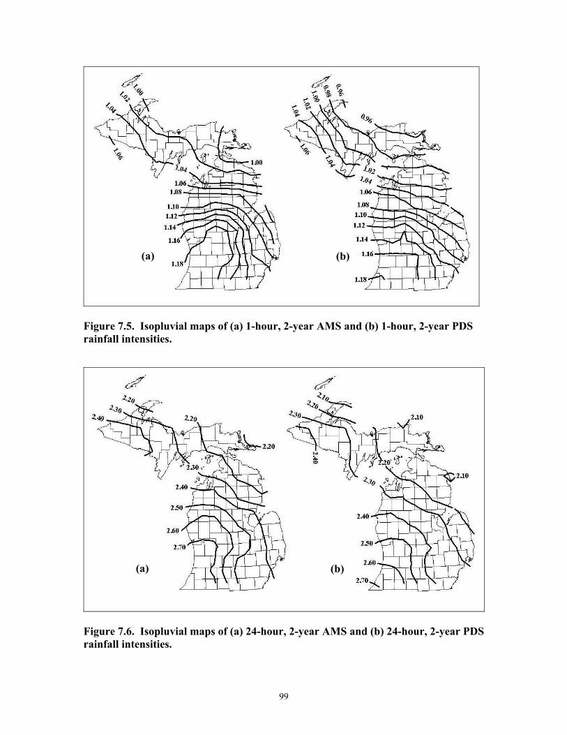
99

Figure 7.5. Isopluvial maps of (a) 1-hour, 2-year AMS and (b) 1-hour, 2-year PDS rainfall intensities.

Figure 7.6. Isopluvial maps of (a) 24-hour, 2-year AMS and (b) 24-hour, 2-year PDS rainfall intensities.

(a) (b)

(a) (b)

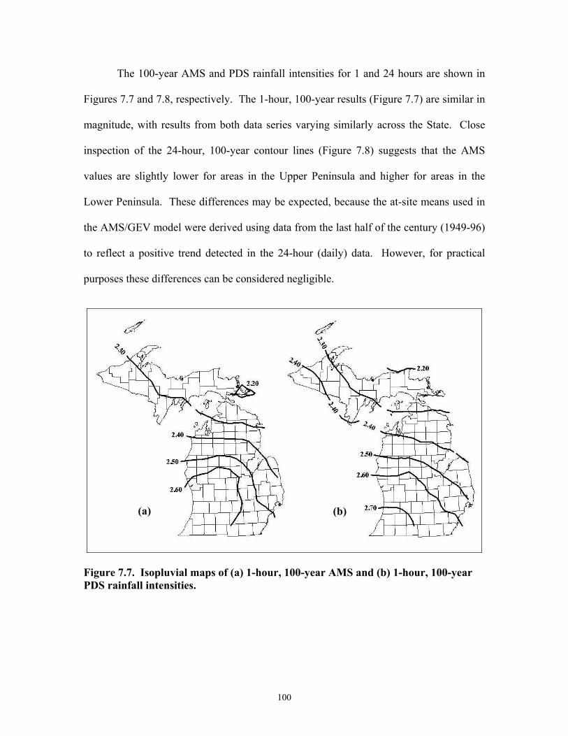
100

The 100-year AMS and PDS rainfall intensities for 1 and 24 hours are shown in

Figures 7.7 and 7.8, respectively. The 1-hour, 100-year results (Figure 7.7) are similar in

magnitude, with results from both data series varying similarly across the State. Close

inspection of the 24-hour, 100-year contour lines (Figure 7.8) suggests that the AMS

values are slightly lower for areas in the Upper Peninsula and higher for areas in the

Lower Peninsula. These differences may be expected, because the at-site means used in

the AMS/GEV model were derived using data from the last half of the century (1949-96)

to reflect a positive trend detected in the 24-hour (daily) data. However, for practical

purposes these differences can be considered negligible.

Figure 7.7. Isopluvial maps of (a) 1-hour, 100-year AMS and (b) 1-hour, 100-year PDS rainfall intensities.

(a) (b)

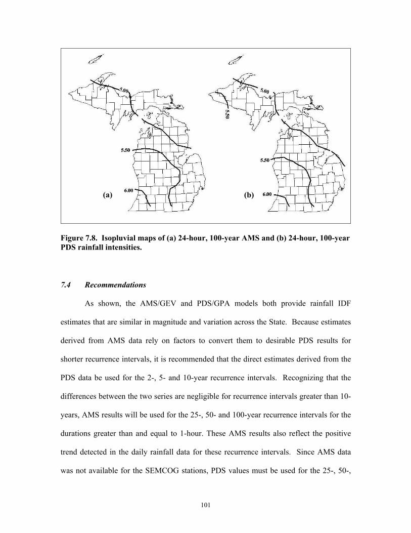
101

Figure 7.8. Isopluvial maps of (a) 24-hour, 100-year AMS and (b) 24-hour, 100-year PDS rainfall intensities.

7.4 Recommendations

As shown, the AMS/GEV and PDS/GPA models both provide rainfall IDF

estimates that are similar in magnitude and variation across the State. Because estimates

derived from AMS data rely on factors to convert them to desirable PDS results for

shorter recurrence intervals, it is recommended that the direct estimates derived from the

PDS data be used for the 2-, 5- and 10-year recurrence intervals. Recognizing that the

differences between the two series are negligible for recurrence intervals greater than 10-

years, AMS results will be used for the 25-, 50- and 100-year recurrence intervals for the

durations greater than and equal to 1-hour. These AMS results also reflect the positive

trend detected in the daily rainfall data for these recurrence intervals. Since AMS data

was not available for the SEMCOG stations, PDS values must be used for the 25-, 50-,

(a) (b)

102

and 100-year recurrence intervals for the short durations (less than 1 hour). These results,

for each of the 10 climatic sections in Michigan, are summarized in tabular form in

Appendix B.

7.5 Comparison with Previous Rainfall Frequency Studies

In 1992, Huff and Angel published Bulletin 71, Rainfall Frequency Atlas of the

Midwest (Huff and Angel, 1992), which updated IDF estimates for nine States in the

Midwest (including Michigan) for 1-hour to 10-day durations and for recurrence intervals

of 2 months to 100 years. Water resources professionals in Michigan often reference the

results of this study. Therefore, the results from Bulletin 71 make for an adequate

comparison to the results derived herein.

Figure 7.9 compares the 1-hour, 2-year results shown in Bulletin 71 with those

derived by the PDS/GPA model. Discrepancies of approximately 0.14 and 0.12 inches

are observed, respectively, in the southwest portion of the Upper Peninsula and the

southwest portion of the Lower Peninsula. Also, intensity values in Bulletin 71 vary

more across the State (0.30 inches) than do those derived from the PDS/GPA model (0.22

inches).

103

Figure 7.9. Comparison of 1-hour, 2-year rainfall intensities based on PDS results for (a) Bulletin 71, and (b) results from the PDS/GPA model.

As shown in Figure 7.10 the differences between the results for the 1-hour

duration are more pronounced at the 100-year recurrence interval. The results derived

from the AMS/GEV model are as much as 0.20 to 0.80 inches lower across the State in

comparison to those from Bulletin 71. Furthermore, the results from Bulletin 71 show a

variation in estimates of 1.5 inches across the State, while the estimates derived from the

AMS/GEV model vary by less than 0.50 inches.

(a) (b)

104

Figure 7.10. Comparison of 1-hour, 100-year rainfall intensities based on AMS results for (a) Bulletin 71, and (b) results from the AMS/GEV model.

The discrepancies noted at the 1-hour duration between the results of this study

and those presented in Bulletin 71 can be explained by the differences in the data used.

In contrast to the hourly-recorded data from 60 stations used for durations less than 24

hours in this study, the results in Bulletin 71 are based on rainfall data collected at 46

daily recording stations. To obtain IDF estimates for durations shorter than 24 hours,

duration-specific conversion factors were applied to the 24-hour estimates. These factors

were based on rainfall data collected in Illinois (34 stations) and adjacent States (21

stations). Also, to obtain 2-year PDS results, Huff and Angel (1992) converted AMS

results to PDS results by a frequency-specific factor (1.13), while the results presented

herein were derived from actual PDS data. Furthermore, data through 1996 were used

herein, while data through only 1986 were used in Bulletin 71. Because of these

(a) (b)

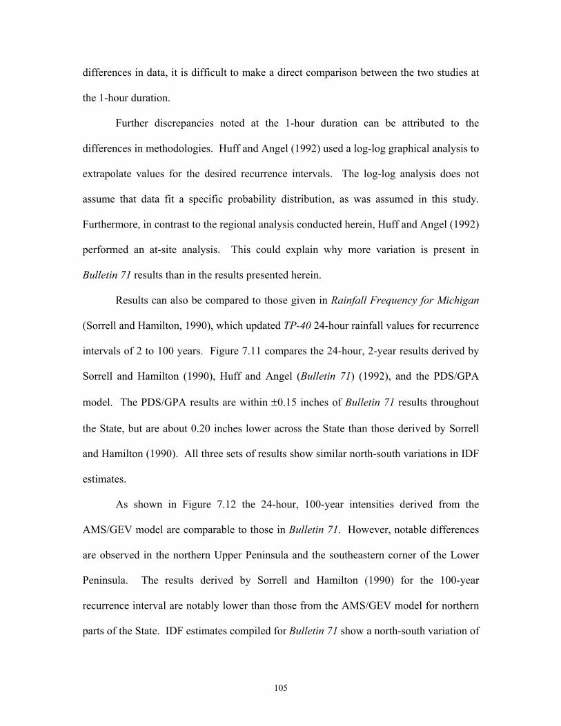
105

differences in data, it is difficult to make a direct comparison between the two studies at

the 1-hour duration.

Further discrepancies noted at the 1-hour duration can be attributed to the

differences in methodologies. Huff and Angel (1992) used a log-log graphical analysis to

extrapolate values for the desired recurrence intervals. The log-log analysis does not

assume that data fit a specific probability distribution, as was assumed in this study.

Furthermore, in contrast to the regional analysis conducted herein, Huff and Angel (1992)

performed an at-site analysis. This could explain why more variation is present in

Bulletin 71 results than in the results presented herein.

Results can also be compared to those given in Rainfall Frequency for Michigan

(Sorrell and Hamilton, 1990), which updated TP-40 24-hour rainfall values for recurrence

intervals of 2 to 100 years. Figure 7.11 compares the 24-hour, 2-year results derived by

Sorrell and Hamilton (1990), Huff and Angel (Bulletin 71) (1992), and the PDS/GPA

model. The PDS/GPA results are within ±0.15 inches of Bulletin 71 results throughout

the State, but are about 0.20 inches lower across the State than those derived by Sorrell

and Hamilton (1990). All three sets of results show similar north-south variations in IDF

estimates.

As shown in Figure 7.12 the 24-hour, 100-year intensities derived from the

AMS/GEV model are comparable to those in Bulletin 71. However, notable differences

are observed in the northern Upper Peninsula and the southeastern corner of the Lower

Peninsula. The results derived by Sorrell and Hamilton (1990) for the 100-year

recurrence interval are notably lower than those from the AMS/GEV model for northern

parts of the State. IDF estimates compiled for Bulletin 71 show a north-south variation of

106

3.0 inches, while those from Sorrell and Hamilton (1990) and those presented herein vary

by less than 2.0 and 1.5 inches, respectively.

Figure 7.11. Comparison of 24-hour, 2-year rainfall intensities based on PDS results from (a) Sorrell and Hamilton (1990), (b) Bulletin 71, and (c) the PDS/GPA model.

Figure 7.12. Comparison of 24-hour, 100-year rainfall intensities based on AMS results from (a) Sorrell and Hamilton (1990), (b) Bulletin 71, and (c) the AMS/GEV model.

(a) (b) (c)

(b)(a) (c)

107

Because all three studies used daily-recorded data to derive rainfall intensities for

the 24-hour duration, a more direct comparison can be made. As previously discussed,

discrepancies between the results of this study and Bulletin 71 IDF estimates can be

attributed to different methodologies used and the fact that 10 more years of data have

been included in this analysis. It should also be noted that the results for Bulletin 71 were

derived from 46 stations with an average record length of 60 years, while this study used

data from 152 stations with an average record length of 63 years. The differences

between the IDF estimates presented by Sorrell and Hamilton (1990) and those of this

study may be explained by the additional 9 to 16 years of data used in this study.

Furthermore, in contrast to the regional approach and the three-parameter GEV and GPA

distributions used herein, Sorrell and Hamilton (1990) derived at-site IDF estimates using

the two-parameter Gumbel distribution and method-of-moments estimators.

7.6 Comparison with Current MDOT IDF Estimates

Currently, the MDOT Road Design Manual (Michigan Department of

Transportation, 1996) provides rainfall intensity values for durations ranging from 10 to

240 minutes and expected recurrence intervals of 10 and 50 years. The State is divided

into 4 zones for these durations and recurrence intervals, as shown in Figure 7.1, with

each zone containing its own representative IDF values. The rationale for the delineation

of these zones is not cited. These estimates are based on those from TP-25 (U.S. Weather

Bureau, 1955) and TP-40 (Hershfield, 1961), but are not taken directly from those

publications.

Comparisons of the current MDOT IDF estimates and the recommended IDF

estimates derived herein for durations of 15 minutes, 1 hour, and 3 hours can be found in

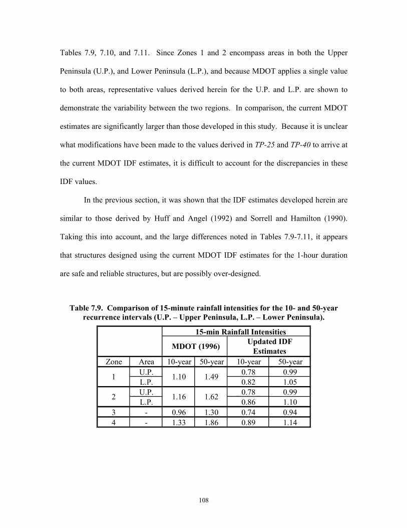
108

Tables 7.9, 7.10, and 7.11. Since Zones 1 and 2 encompass areas in both the Upper

Peninsula (U.P.), and Lower Peninsula (L.P.), and because MDOT applies a single value

to both areas, representative values derived herein for the U.P. and L.P. are shown to

demonstrate the variability between the two regions. In comparison, the current MDOT

estimates are significantly larger than those developed in this study. Because it is unclear

what modifications have been made to the values derived in TP-25 and TP-40 to arrive at

the current MDOT IDF estimates, it is difficult to account for the discrepancies in these

IDF values.

In the previous section, it was shown that the IDF estimates developed herein are

similar to those derived by Huff and Angel (1992) and Sorrell and Hamilton (1990).

Taking this into account, and the large differences noted in Tables 7.9-7.11, it appears

that structures designed using the current MDOT IDF estimates for the 1-hour duration

are safe and reliable structures, but are possibly over-designed.

Table 7.9. Comparison of 15-minute rainfall intensities for the 10- and 50-year recurrence intervals (U.P. – Upper Peninsula, L.P. – Lower Peninsula).

Zone Area 10-year 50-year 10-year 50-yearU.P. 0.78 0.99L.P. 0.82 1.05U.P. 0.78 0.99L.P. 0.86 1.10

3 - 0.96 1.30 0.74 0.944 - 1.33 1.86 0.89 1.14

1.10 1.49

1.16 1.62

Updated IDFEstimatesMDOT (1996)

15-min Rainfall Intensities

1

2

109

Table 7.10. Comparison of 1-hour rainfall intensities for the 10- and 50-year recurrence intervals (U.P. – Upper Peninsula, L.P. – Lower Peninsula).

Zone Area 10-year 50-year 10-year 50-yearU.P. 1.55 2.05L.P. 1.65 2.20U.P. 1.60 2.10L.P. 1.78 2.35

3 - 1.77 2.44 1.50 2.054 - 2.44 3.54 1.80 2.40

2.03 2.82

2.17 3.07

Updated IDFEstimatesMDOT (1996)

1-hour Rainfall Intensities

1

2

Table 7.11. Comparison of 3-hour rainfall intensities for the 10- and 50-year recurrence intervals (U.P. – Upper Peninsula, L.P. – Lower Peninsula).

Zone Area 10-year 50-year 10-year 50-yearU.P. 1.98 2.56L.P. 2.08 2.71U.P. 1.98 2.56L.P. 2.19 2.83

3 - 2.24 2.94 1.93 2.514 - 2.95 4.37 2.29 2.96

2.48 3.43

2.60 3.78

Updated IDFEstimatesMDOT (1996)

3-hour Rainfall Intensities

1

2

7.7 Verification of Results

To partially verify the developed IDF estimates, one can compare the T-year

event estimate to those events actually observed. The probability, R, of measuring a T-

year event or greater at a site with record length n, can be calculated as

.111n

TR

−−=

(7.1)

110

For a region with N stations, the expected number of stations with observed exceedances

can be approximated as

RN * Stations of No. Expected ≈ (7.2) where R is computed using the average record length in the region.

This has been done for the seven longer durations (greater than and equal to an

hour) by comparing the estimated AMS 100-year event to the observed maximum at each

recording station. For the four short-duration stations (less than an hour), this was done

by comparing the estimated PDS 100-year event to the observed maximum at each

recording station. For each duration the ratio of the number of stations that have

observed exceedances (X) and the number of stations expected to observe exceedances

(N*R) has been calculated, as shown in column (7) of Table 7.10. Additionally, the

probability of observing X or more stations with exceedances due to chance alone is

shown in column (8) of Table 7.10. This probability was calculated using the cumulative

binomial distribution function (DeGroot, 1989) as follows:

( ) ( ) XNX RRN

XRNXB −−

= ∑ 1,,

(7.3)

).,,(1)( RNXBxXP −=>= (7.4)

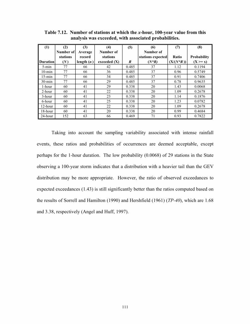
111

Table 7.12. Number of stations at which the x-hour, 100-year value from this analysis was exceeded, with associated probabilities.

(1)

Duration

(2)Number of

stations (N )

(3)Average record

length (n )

(4)Number of

stations exceeded (X)

(5)

R

(6)Number of

stations expected (N*R)

(7)

Ratio (X/(N*R ))

(8)

Probability (X >= x)

5-min 77 66 42 0.485 37 1.12 0.119410-min 77 66 36 0.485 37 0.96 0.574915-min 77 66 34 0.485 37 0.91 0.740630-min 77 66 29 0.485 37 0.78 0.96351-hour 60 41 29 0.338 20 1.43 0.00682-hour 60 41 22 0.338 20 1.09 0.26783-hour 60 41 23 0.338 20 1.14 0.18766-hour 60 41 25 0.338 20 1.23 0.078212-hour 60 41 22 0.338 20 1.09 0.267818-hour 60 41 20 0.338 20 0.99 0.468424-hour 152 63 66 0.469 71 0.93 0.7822

Taking into account the sampling variability associated with intense rainfall

events, these ratios and probabilities of occurrences are deemed acceptable, except

perhaps for the 1-hour duration. The low probability (0.0068) of 29 stations in the State

observing a 100-year storm indicates that a distribution with a heavier tail than the GEV

distribution may be more appropriate. However, the ratio of observed exceedances to

expected exceedances (1.43) is still significantly better than the ratios computed based on

the results of Sorrell and Hamilton (1990) and Hershfield (1961) (TP-40), which are 1.68

and 3.38, respectively (Angel and Huff, 1997).

112

8.0 SUMMARY AND CONCLUSION

Using data from 76 hourly and 152 daily rainfall-recording stations throughout

Michigan, along with 81 Southeast Michigan Council of Governments (SEMCOG) short

duration rainfall-recording stations located in 5 counties in and around the Detroit area,

spatially varying rainfall intensity estimates were determined for each of eleven durations

(5, 10, 15, 30, 60, 120, 180, 360, 720, 1080, and 1440 minutes) and six recurrence

intervals (2, 5, 10, 25, 50 and 100 years). Both AMS and PDS data were compiled,

where available, from gages with records ranging from 16 to 117 years in length.

Recommended IDF estimates for 5 to 30 minutes were based on the SEMCOG data,

estimates for 1 to 18 hours were derived from hourly records, and 24-hour estimates were

derived from daily records.

All data were screened for gross errors by the State Climatologist, and additional

checks were made using a discordancy measure. Trend analyses generally indicated

increasing trends in the data (i.e., more intense storms, or more frequent storms of a given

intensity, in recent years), but only in the case of the 24-hour AMS data was the trend

found to be significant. A procedure for adjusting for this trend was suggested.

The frequency analysis procedure followed was the Regional L-Moment

Algorithm, which is described by Hosking and Wallis (1997) and is being applied by the

National Weather Service in other parts of the US. This procedure assumes that sites

from a homogeneous region have an identical frequency distribution apart from a site-

specific scaling factor. It was found reasonable to consider the State of Michigan as a

single homogeneous region, with the mean of each site-specific data series (either AMS

113

or PDS) used as the scaling factor. Spatial interpolation of these site-specific factors

through kriging allowed production of isopluvial maps that resemble previously used

maps of rainfall intensities.

Based on goodness-of-fit statistics, the frequency distributions selected were the

GEV distribution for the AMS data and the GPA distribution for the PDS data. These

distributions not only provided a good fit to the data, but are expected to reliable and

robust quantile estimates. Upon estimation of distribution parameters using L-moments,

quantile (IDF) estimates were computed for regions throughout the state. The

recommended IDF estimates are tabulated for the state’s 10 NWS climatic sections

(Appendix B), and are also illustrated in isopluvial maps (Appendix C).

The recommended IDF estimates were compared to the results of previous studies

and to the design IDF values currently used by MDOT. In general, the results of this

study were more similar to those presented in Bulletin 71, Rainfall Frequency Atlas of the

Midwest (Huff and Angel, 1992) and Rainfall Frequency for Michigan (Sorrell and

Hamilton, 1990) than to the IDF values given in the MDOT Road Design Manual,

although discrepancies among all four sets of values were significant. Most notably, it

was found that current MDOT estimates are significantly larger than those developed in

this study. For instance, for 1-hour storms, current MDOT estimates of 10-year rainfall

depths now appear to be closer to 50-year depths. Because it is unclear how the current

MDOT IDF estimates were derived, based on adjustments to values derived in TP-25 and

TP-40, it was not possible to account for these discrepancies. However, based on

verification results which indicated that the revised IDF estimates lead to approximately

the number of exceedances that would be expected statistically over the period of record,

114

it appears that structures designed using the current MDOT IDF estimates are safe and

reliable structures, but are possibly over-designed.

115

References ArcInfo GIS version 7.2.1 (1998). Environmental Systems Research Institute, Inc. Redlands, CA. ArcView GIS version 3.1 (1998). Environmental Systems Research Institute, Inc. Redlands, CA. Armstrong, M. (1998). Basic Linear Geostatistics. Heidelburg, Germany: Springer-Verlag Berlin. Angel, J.R. and Huff, F.A. (1997). Changes in Heavy Rainfall in Midwestern United States. Journal of Water Resources Planning and Management. 123.4: 246-249. Bates, B.C., A. Rahman, R.G. Mein, and P.E. Weinmann (1998). “Climatic and physical factors that influence the homogeneity of regional floods in southeastern Australia,” Water Resourc. Res., vol. 34, no. 12, pp. 3369-3381. Burrough, Peter A. and McDonnell, Rachael A. (1998). Principles of Geographical Information Systems: Spatial Information Systems and Geostatistics. Oxford, NY: Oxford University Press. Clark, Isobel (1987). Practical Geostatistics. Essex, England: Elsevier Applied Science Publishers LTD. Cressie, N.A.C. (1991). Statistics for Spatial Data. New York, NY: John Wiley and Sons, Inc. Dalrymple, T. (1960). “Flood Frequency Analyses,” Water Supply Paper 1543-A, U.S.G.S., Reston, VA. DeGroot, M.A. (1986). Probability and Statistics. 3rd Edition. Reading, MA: Addison-Wesley Publishing Company, Inc. Deutsch, C.V., and Journel, A.G. (1998). GSLIB: Geostatistical Software Library and User’s Guide. 2nd Edition. New York, NY: Oxford University Press. Dunn, C. N. (1986). “Generation of Regional Rainfall Intensity-Duration-Frequency Curves for Pennsylvania,” M.S. Thesis, Dept. of Civil Engineering, Pennsylvania State University, College Station, PA. Fovell, R.G., and M.-Y. C. Fovell (1993). “Climate Zones of the Conterminous United States Defined Using Cluster Analysis,” Journal of Climate, vol. 6, pp. 2103-2135.

116

Frederick, R.H., Meyers, V.A., and Auciello, E.P. (1977). Five- to 60-Minute Precipitation Frequency for the Eastern and Central United States. NOAA Technical Memorandum U.S. National Weather Service, Washington, D.C. Greenwood, J.A., J.M. Landwehr, N.C. Matalas, and J.R. Wallis (1979). “Probability Weighted Moments: Definitions and Relation to Parameters of Several Distributions Expressible in Inverse Form,” Water Resourc. Res., vol. 15, no. 6, pp. 1049-1054. Hartigan, J.A., and M.A. Wong (1979). “Algorithm AS 136: A K-Means Clustering Algorithm,” Applied Statistics, vol. 28, pp. 100-108. Hershfield, D.M. (1961). Rainfall Frequency Atlas for the United States for Durations from 30 Minutes to 24 Hours and Return Periods from 1 to 100 Years. U.S. Weather Bureau Technical Paper 40, Washington, D.C. Hirsch, R.M., and D.R. Helsel, T.A. Cohn, and E.J. Gilroy (1993). “Statistical Analysis of Hydrological Data,” Chapter 17 in Handbook of Hydrology, ed. D.R. Maidment, McGraw-Hill, New York. Hohn, M.A. (1988). Geostatistics and Petroleum Geology. New York, NY: Van Norstrand Reinhold. Hosking, J.R.M., J.R. Wallis and E.F. Wood (1985). “Estimation of the Generalized-ExtremeValue Distribution by the Method of Probability-Weighted Moments,” Technometrics, vol. 27, no. 3, pp. 251-261. Hosking, J.R.M., and J.R. Wallis (1987). “Parameter and Quantile Estimation for the Generalized Pareto Distribution,” Technometrics, vol. 29, no. 3, pp. 339-349. Hosking, J.R.M., and J.R. Wallis (1988). “The effect of intersite dependence on regional flood frequency analysis,” Water Resourc. Res., vol. 24, no. 4, pp. 588-600. Hosking, J.R.M. (1990). “L-moments: Analysis and Estimation of Distributions using Linear Combinations of Order Statistics,” J.R. Statist. Soc., B, vol. 52, no. 1, pp. 105-124. Hosking, J.R.M., and J.R. Wallis (1996). “The U.S. National Electronic Drought Atlas: Statistical Data Analysis with GIS-Based Presentation of Results,” research report RC-20499, IBM Research Division, T.J. Watson Research Center, Yorktown Heights, N.Y. Hosking, J.R.M. (1997). “Fortran Routines for Use with the Method of L-Moments, Version 3.02,” research report RC-20525, IBM Research Division, T.J. Watson Research Center, Yorktown Heights, N.Y. Hosking, J.R.M. and Wallis, J.R. (1997). Regional Frequency Analysis: An Approach Based on L-moments. Cambridge, UK: Cambridge University Press.

117

Huff, F.A., and J.C. Neill (1959). “Frequency Relations for Storm Rainfall in Illinois,” Illinois State Water Survey, Bulletin 46, Urbana, IL. Huff, F.A. (1975). “Urban Effects on the Distribution of Heavy Convective Rainfall,” Water Resour. Res., vol. 11, no. 6, pp. 889-896. Huff, F.A., and S.A. Changnon (1987). “Temporal Changes in Design Rainfall Frequencies in Illinois,” Climate Change, vol. 10, pp. 195-200. Huff, F. A. and Angel, J. R. (1989). Frequency Distributions and Hydroclimatic Characteristics of Heavy Rainstorms in Illinois. Illinois State Water Survey, Bulletin 70, Champaign, Illinois. Huff, F.A., and J.R. Angel (1990). “Fluctuations in the Frequency Distributions of Heavy Rainstorms in the Midwest,” Preprint, American Meteorological Society Symposium on Global Change Systems, Anaheim, CA. Huff, F. A. and Angel, J.R. (1992). Rainfall Frequency Atlas of the Midwest. Illinois State Water Survey, Bulletin 71, Champaign, Illinois. Journel, A.G. and Huijbregts, CH.J. (1978). Mining Geostatistics. New York, NY: Academic Press Inc. Julian, L.T., B. Lin, J.M. Daniel, T. Davila, S.M. Gillete and M. Yekta (1998). “Ohio River Basin Precipitation Frequency Study, Update of Technical Paper 40, Second Progress Report,” Office of Hydrology, U.S. National Weather Service, Silver Spring, MD. Julian, L.T., B. Lin, J.M. Daniel and M. Yetka (1999). “Ohio River Basin Precipitation Frequency Study, Update of Technical Paper 40, Third Progress Report,” Office of Hydrology, U.S. National Weather Service, Silver Spring, MD. Julian, L.T., J. Daniel, B. Lin, D. Riley, and M. Yetka (March 2000). “Ohio River Basin Precipitation Frequency Study, Update of Technical Paper 40, Fourth Progress Report,” Office of Hydrology, U.S. National Weather Service, Silver Spring, MD. Julian, L.T., B. Lin, E. Raynault, D. Riley, D. Todd, and M. Yetka (September 2000). “Ohio River Basin Precipitation Frequency Study, Update of Technical Paper 40, Fifth Progress Report,” Office of Hydrology, U.S. National Weather Service, Silver Spring, MD. Julian, L.T., et. al. (April 2001). “Ohio River Basin Precipitation Frequency Study, Update of Technical Paper 40, Sixth Progress Report,” Office of Hydrology, U.S. National Weather Service, Silver Spring, MD.

118

Julian, L.T., et. al. (July 2001). “Ohio River Basin Precipitation Frequency Study, Update of Technical Paper 40, Seventh Progress Report,” Office of Hydrology, U.S. National Weather Service, Silver Spring, MD. Karl, T.R., R.W. Knight, D.R. Easterling, and R.G. Quayle (1996). “Indices of Climate Change for the United States,” Bull. of the Amer. Meteorolog. Soc., vol. 77, no. 2, pp. 279-292. Karl, T.R. and R.W. Knight (1998). “Secular Trends of Precipitation Amount, Frequency, and Intensity in the United States,” Bull. of the Amer. Meteorolog. Soc., vol. 79, no. 2, pp. 231-241. Kitanidis, Peter K. (1993). “Geostatistics,” Chapter 20 in Handbook of Hydrology, Maidment, David R. eds. New York, NY: McGraw-Hill. Kunkel, K.E., K. Andsager, and D.R. Easterling (1999). “Long-Term Trends in Extreme Precipitation Events over the Conterminous United States and Canada,” Journal of Climate, vol. 12, pp. 2515-2527. Lancaster, Peter and Salkauskas, Kestutis (1986). Curve and Surface Fitting: An Introduction. London, UK: Academic Press. Landwehr, J.M., N.C. Matalas, and J.R. Wallis (1979). “Probability Weighted Moments Compared with Some Traditional Techniques in Estimating Gumbel Parameters and Quantiles,” Water Resourc. Res., vol. 15, no. 5, pp. 1055–1064. Lettenmaier, D.P., J.R. Wallis, and E.F. Wood (1987). “Effect of regional heterogeneity on flood frequency estimation,” Water Resourc. Res., vol. 23, pp. 313-323. Loucks, E., C. Rodgers, K. Potter, and M.G. Hahn (2000). “Technical Report Number 40: Rainfall Frequency in the Southeastern Wisconsin Region,” Southeastern Wisconsin Regional Planning Commission, Waukesha, WI. Madsen, H., and D. Rosbjerg (1997). “The partial duration series method in regional index-flood modeling,” Water Resour. Res., vol. 33, no. 4, pp. 737-746. Madsen, H., C.P. Pearson, and D. Rosbjerg (1997). “Comparison of Annual Maximum Series and Partial Duration Series Methods for Modeling Extreme Hydrologic Events, 2. Regional Modeling,” Water Resour. Res., vol. 33, no. 4, pp. 759-769. Madsen, H., P.S. Mikkelsen, D. Rosbjerg, and P. Harremoës (1998). “Estimation of Regional Intensity-Duration-Frequency Curves for Extreme Precipitation,” Wat. Sci. Tech., vol. 37, no. 11, pp. 29-36. Maidment, D.R. (1993). “GIS and Hydrologic Modeling,” Chapter 14 in Environmental Modeling with GIS, M.F. Goodchild, B.O. Parks, and L.F. Steyaert, eds. New

119

York, NY: Oxford University Press. Michigan Department of Transportation (1996). Michigan Design Manual: Road Design, vol. 3, sections 4.02.04 & 4.02.05, Michigan Department of Transportation, Lansing, MI. Miller, J.F., Frederick, R.H. and Tracey, R.J. (1973). Precipitation-Frequency Atlas of the Western United States. NOAA Atlas II, National Weather Service, Silver Springs, MD. Potter, K.W., and D.P. Lettenmaier (1990). “A comparison of regional flood frequency estimation methods using a resampling method,” Water Resour. Res., vol. 26, pp. 415-424. Rosbjerg, D. (1985). “Estimation in Partial Duration Series with Independent and Dependent Peak Values,” Journal of Hydrology, vol. 76, pp. 183-195. Schaefer, M.G. (1990). “Regional Analyses of Precipitation Annual Maxima in Washington State,” Water Resour. Res., vol. 26, no. 1, pp. 119-131. Sorrell, R.C., and Hamilton, D.A. (1990). Rainfall Frequency for Michigan: 24-hour Duration with Return Periods from 2 to 100 Years. Michigan Department of Natural Resources: Land and Management Division. Stedinger, J.R., R.M. Vogel and E. Foufoula-Georgiou (1993). “Frequency Analysis of Extreme Events,” Chapter 18 in Handbook of Hydrology, ed. D.R. Maidment, McGraw-Hill, New York. Tavares, L.V., and J.E. Da Silva (1983). “Partial Duration Series Revisited,” Journal of Hydrology, vol. 64, pp. 1-14. U.S. Weather Bureau (1955). Rainfall Intensity-Duration-Frequency Curves for Selected Stations in the United States, Alaska, Hawaiian Islands, and Puerto Rico. Technical Paper 25. Washington, D.C. Wallis, J.R., N.C. Matalas and J.R. Slack (1974). “Just a Moment!,” Water Resourc. Res., vol. 10, no. 2, pp. 211-219. Watson, David F. (1992). Contouring: A Guide to the Analysis and Display of Spatial Data. Oxford, UK: Elsevier Science Ltd. Wingle, W.L., Poeter, E.P., and McKenna, S.A. (1995). UNCERT: A Geostatistical Uncertainty Analysis Package Applied to Groundwater Flow and Contaminant Transport Modeling, Colorado School of Mines. http://uncert.mines.edu/ Yarnell, D.L. (1935). “Rainfall Intensity-Frequency Data,” Miscellaneous Publication No. 204, U.S. Department of Agriculture, Washington D.C.

120

Appendix A Recording Station Data

Table A.1. Properties of selected hourly recording stations (shading indicates those that have been combined with another station).

S tation N am e S tation ID

Y ears of R ecord L atitu d e (N ) L on g itu d e (W )

A llegan 5 N E 128 48 42 .58 -85 .78A lpena W S O A irpo rt 164 36 45 .07 -83 .57A nn A rbor U o f M 230 49 42 .30 -83 .72B araga 1 N 489 38 46 .78 -88 .48B eaverton P ow er P lan t 631 28 43 .88 -84 .48B ella ire 662 49 44 .98 -85 .20B errien S prings 5 W 735 49 41 .97 -86 .43B ig B ay 8 N W 766 36 46 .88 -87 .87B row n C ity 5 S S W 1054 26 43 .12 -82 .98B ruce C rossing 1088 49 46 .53 -89 .18B urnside 1 E 1133 24 43 .20 -83 .05C asnov ia 2 N W 1352 37 43 .25 -85 .82C hatham E x perim ent F arm 1486 23 46 .33 -86 .92C heboygan 1492 47 45 .65 -84 .47C o ldw ater W W T P 1680 49 41 .93 -85 .02C o lom a 3 N N W 1704 49 42 .23 -86 .32C opper H arbo r F ort W ilk ins 1780 49 47 .47 -87 .87C rysta l Fa lls 6 N E 1922 42 46 .17 -88 .23D e T our V illage 2094 49 45 .98 -83 .90D etro it C ity A irport 2102 49 42 .42 -83 .02D etro it M etro W S C M O 2103 38 42 .23 -83 .32E ast Lansing 4 S 2395 40 42 .67 -84 .48E scanaba 2626 47 45 .75 -87 .03F ife Lake 1 N N W 2788 42 44 .58 -85 .35Flin t W S C M O 2846 39 42 .97 -83 .75G ladw in 3170 21 43 .98 -84 .50G lenn ie A lcona D am 3199 48 44 .57 -83 .80G rand H aven W W T P 3295 49 43 .07 -86 .20G rand R ap ids W S F O 3333 33 42 .88 -85 .52G w inn 1 W 3516 47 46 .28 -87 .45H ancock M cLain S tate P ark 3551 45 47 .23 -88 .62H arbor B each 3580 49 43 .83 -82 .65H ough ton Lake W S O A P 3936 33 44 .37 -84 .68H ow ell W W T P 3947 47 42 .60 -83 .93Iron M tn -K ingsfo rd W 4090 49 45 .78 -88 .08Jackson 3 N 4155 49 42 .28 -84 .42K alam azoo S tate H osp ital 4244 43 42 .29 -85 .60K enton 4328 47 46 .48 -88 .50Lansing W S O A irport 4641 45 42 .77 -84 .60Lud ington S ta te P ark 4959 49 44 .03 -86 .50Lup ton 4 S 4966 19 44 .38 -84 .05M arquette 5178 31 46 .55 -87 .38M arquette W S O 5184 18 46 .53 -87 .55M ontague 4 N W 5567 49 43 .47 -86 .42M uskegon W S O A irpo rt 5712 49 43 .17 -86 .25N ew berry 3 S 5816 46 46 .32 -85 .50O ntonagon 6215 48 46 .85 -89 .30O w osso W W T P 6300 41 43 .02 -84 .18R oscom m on 7122 41 44 .50 -84 .60R ose C ity 7134 19 44 .43 -84 .12S au lt S te M arie W S O 7366 49 46 .47 -84 .35S ebew aing 7419 37 43 .73 -83 .45S tan ton 7828 39 43 .28 -85 .10S teuben 7880 42 46 .18 -86 .47T raverse C ity 8246 39 44 .77 -85 .57T rou t Lake 8293 46 46 .20 -85 .02V anderb ilt 11 E N E 8417 49 45 .17 -84 .45V assar 8443 38 43 .37 -83 .58

121

Table A.2. Properties of selected daily recording stations.

Station Name Station ID

Years of Record Latitude (N) Longitude (W)

ADRIAN 2 NNE 32 110 41.92 -84.02ALBERTA FFC 89 41 46.65 -88.48ALBION 94 49 42.25 -84.77ALLEGAN 5 NE 128 109 42.58 -85.78ALMA 146 110 43.38 -84.67ALPENA WSO AIRPORT 164 81 45.07 -83.58ALPENA WWTP 169 49 45.07 -83.43ANN ARBOR U OF M 230 117 42.30 -83.72ATLANTA 5 WNW 343 70 45.03 -84.23BAD AXE 417 72 43.82 -83.00BALDWIN 446 61 43.90 -85.85BARAGA 1 N 489 24 46.78 -88.48BATTLE CREEK 5 NW 552 102 42.37 -85.27BEECHWOOD 7 WNW 647 42 46.18 -88.88BENTON HARBOR ARPT 710 110 42.13 -86.43BERGLAND DAM 718 59 46.58 -89.55BIG BAY 2 SE 770 28 46.80 -87.70BIG RAPIDS WATERWORKS 779 101 43.70 -85.48BLOOMINGDALE 864 92 42.38 -85.97BOYNE FALLS 925 48 45.17 -84.92CADILLAC 1176 88 44.27 -85.40CARO REGIONAL CENTER 1299 69 43.45 -83.40CHAMPION VAN RIPER SP 1439 48 46.52 -87.98CHARLEVOIX 1468 49 45.32 -85.27CHARLOTTE 1476 95 42.55 -84.83CHATHAM EXP. FARM 1484 92 46.35 -86.93CHEBOYGAN 1492 106 45.65 -84.47COLDWATER STATE SCHL 1675 100 41.95 -85.00CORNELL 4 WSW 1800 30 45.88 -87.30CROSS VILLAGE 1896 44 45.63 -85.03CRYSTAL FALLS 6 NE 1922 42 46.17 -88.23DEARBORN 2015 45 42.32 -83.23DETOUR VILLAGE 2094 49 45.99 -83.90DETROIT CITY AIRPORT 2102 33 42.42 -83.02DETROIT METRO WSCMO 2103 99 42.22 -83.35DOWAGIAC 1 W 2250 49 41.98 -86.13DUNBAR FOREST EXP ST 2298 44 46.32 -84.23EAGLE HARBOR 2332 25 47.47 -88.17EAST JORDAN 2381 68 45.15 -85.13EAST LANSING EXPERIM 2393 51 42.70 -84.47EAST LANSING WB CITY 2394 48 42.73 -84.48EAST LANSING 4 S 2395 87 42.67 -84.48EAST TAWAS 2423 65 44.28 -83.50EATON RAPIDS 2437 49 42.52 -84.65EAU CLAIRE 4 NE 2445 73 42.02 -86.25ESCANABA 2626 47 45.75 -87.03ESSEXVILLE 2631 101 43.62 -83.87EVART 2671 47 43.92 -85.27FAYETTE 4 SW 2737 66 45.67 -86.72FIFE LAKE 4 SW 2784 36 44.55 -85.42

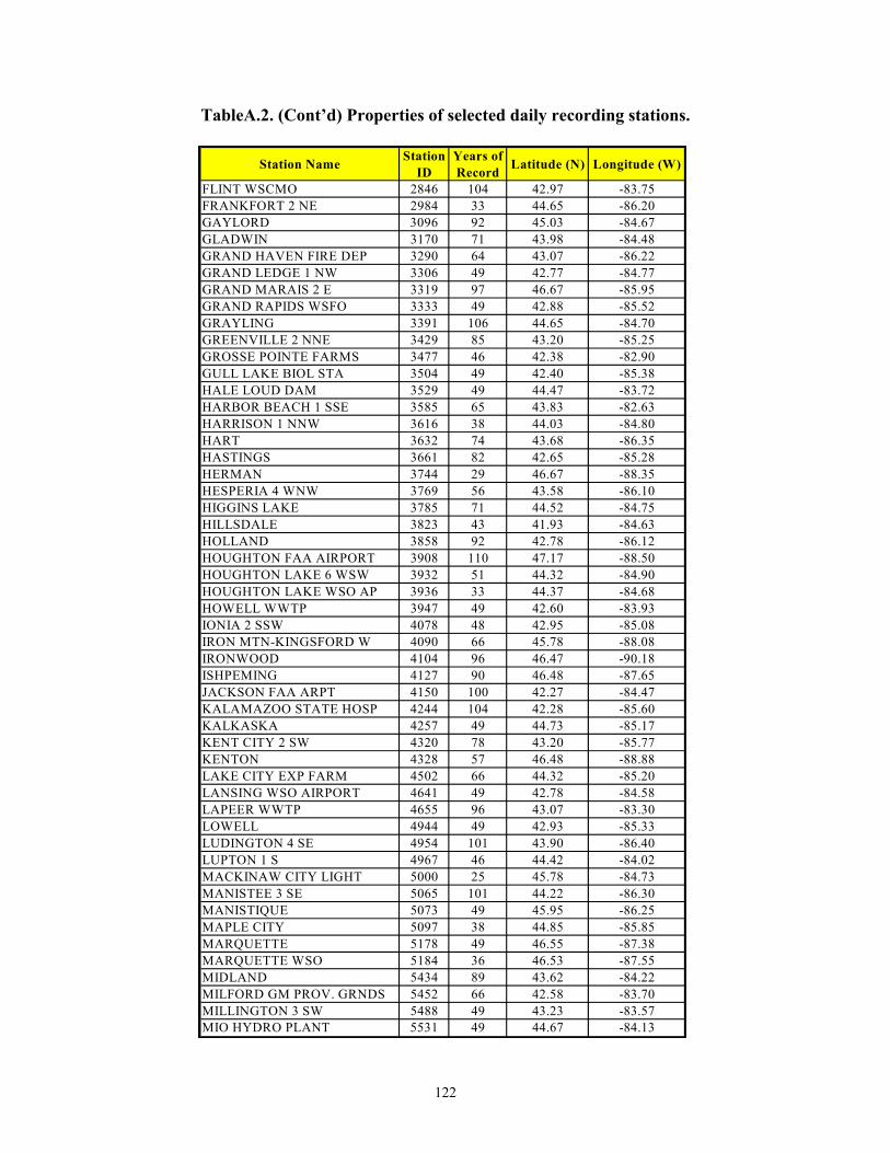
122

TableA.2. (Cont’d) Properties of selected daily recording stations.

Station Name Station ID

Years of Record Latitude (N) Longitude (W)

FLINT WSCMO 2846 104 42.97 -83.75FRANKFORT 2 NE 2984 33 44.65 -86.20GAYLORD 3096 92 45.03 -84.67GLADWIN 3170 71 43.98 -84.48GRAND HAVEN FIRE DEP 3290 64 43.07 -86.22GRAND LEDGE 1 NW 3306 49 42.77 -84.77GRAND MARAIS 2 E 3319 97 46.67 -85.95GRAND RAPIDS WSFO 3333 49 42.88 -85.52GRAYLING 3391 106 44.65 -84.70GREENVILLE 2 NNE 3429 85 43.20 -85.25GROSSE POINTE FARMS 3477 46 42.38 -82.90GULL LAKE BIOL STA 3504 49 42.40 -85.38HALE LOUD DAM 3529 49 44.47 -83.72HARBOR BEACH 1 SSE 3585 65 43.83 -82.63HARRISON 1 NNW 3616 38 44.03 -84.80HART 3632 74 43.68 -86.35HASTINGS 3661 82 42.65 -85.28HERMAN 3744 29 46.67 -88.35HESPERIA 4 WNW 3769 56 43.58 -86.10HIGGINS LAKE 3785 71 44.52 -84.75HILLSDALE 3823 43 41.93 -84.63HOLLAND 3858 92 42.78 -86.12HOUGHTON FAA AIRPORT 3908 110 47.17 -88.50HOUGHTON LAKE 6 WSW 3932 51 44.32 -84.90HOUGHTON LAKE WSO AP 3936 33 44.37 -84.68HOWELL WWTP 3947 49 42.60 -83.93IONIA 2 SSW 4078 48 42.95 -85.08IRON MTN-KINGSFORD W 4090 66 45.78 -88.08IRONWOOD 4104 96 46.47 -90.18ISHPEMING 4127 90 46.48 -87.65JACKSON FAA ARPT 4150 100 42.27 -84.47KALAMAZOO STATE HOSP 4244 104 42.28 -85.60KALKASKA 4257 49 44.73 -85.17KENT CITY 2 SW 4320 78 43.20 -85.77KENTON 4328 57 46.48 -88.88LAKE CITY EXP FARM 4502 66 44.32 -85.20LANSING WSO AIRPORT 4641 49 42.78 -84.58LAPEER WWTP 4655 96 43.07 -83.30LOWELL 4944 49 42.93 -85.33LUDINGTON 4 SE 4954 101 43.90 -86.40LUPTON 1 S 4967 46 44.42 -84.02MACKINAW CITY LIGHT 5000 25 45.78 -84.73MANISTEE 3 SE 5065 101 44.22 -86.30MANISTIQUE 5073 49 45.95 -86.25MAPLE CITY 5097 38 44.85 -85.85MARQUETTE 5178 49 46.55 -87.38MARQUETTE WSO 5184 36 46.53 -87.55MIDLAND 5434 89 43.62 -84.22MILFORD GM PROV. GRNDS 5452 66 42.58 -83.70MILLINGTON 3 SW 5488 49 43.23 -83.57MIO HYDRO PLANT 5531 49 44.67 -84.13

123

Table A.2. (Cont’d) Properties of selected daily recording stations.

Station Name Station ID

Years of Record Latitude (N) Longitude (W )

MONROE 5558 80 41.92 -83.40MONTAGUE 4 NW 5567 47 43.47 -86.42MOTT ISLAND ISLE ROY 5637 45 48.10 -88.55MOUNT CLEMENS ANG BA 5650 63 42.62 -82.83MT PLEASANT UNIV 5662 98 43.58 -84.77MUNISING 5690 53 46.42 -86.67MUSKEGON W SO AIRPORT 5712 101 43.17 -86.23NEW BERRY 3 S 5816 101 46.32 -85.50NILES 5892 49 41.83 -86.27ONAW AY STATE PARK 6184 49 45.43 -84.23OW OSSO W W TP 6300 97 43.02 -84.18PELLSTON AIRPORT 6438 49 45.57 -84.78PETOSKEY 6507 45 45.37 -84.98PONTIAC STATE HOSPIT 6658 89 42.65 -83.30PORT HURON 6680 66 42.98 -82.42PORT INLAND 6686 37 45.97 -85.87ROCK 1 E 7068 43 46.07 -87.15ROGERS CITY 3 S 7089 26 45.38 -83.83RUDYARD 4 N 7190 49 46.30 -84.58SAGINAW CONSUMERS PW 7217 33 43.45 -83.97SAGINAW FAA AIRPORT 7227 101 43.53 -84.08SAINT CHARLES 7253 33 43.30 -84.17ST IGNACE MACKINAC B 7274 24 45.85 -84.72ST JAMES 2 S BEAVER 7277 40 45.72 -85.52ST JOHNS 7280 59 43.02 -84.55SANDUSKY 7350 46 43.42 -82.82SAULT STE MARIE W SO 7366 58 46.47 -84.35SCOTTVILLE 1 NE 7405 31 43.97 -86.27SEBEW AING 7419 43 43.73 -83.45SENEY W ILDLIFE REFUG 7515 49 46.28 -85.95SOUTH HAVEN 7690 71 42.40 -86.28SPALDING 1 SSE 7742 44 45.68 -87.50STAMBAUGH 2 SSE 7812 98 46.05 -88.62STANDISH 5 SW 7820 59 43.95 -84.03STEPHENSON 8 W NW 7867 49 45.45 -87.75STEUBEN 7880 42 46.18 -86.47SUTTONS BAY 4 NW 8032 21 45.02 -85.70TAHQUAMENON FALLS ST 8043 24 46.60 -85.22THOMPSONVILLE 8167 36 44.52 -85.93THREE RIVERS 8184 54 41.93 -85.63TRAVERSE CITY FAA AP 8251 101 44.73 -85.58VANDERBILT 11 ENE 8417 66 45.17 -84.43W ASHINGTON 8650 39 42.73 -83.03W ATERSMEET 8680 59 46.28 -89.17W ELLSTON TIPPY DAM 8772 49 44.25 -85.93W EST BRANCH 3 SE 8800 97 44.25 -84.20W HITEFISH POINT 8920 79 46.75 -84.98W ILLIAMSTON 3 NE 9006 44 42.72 -84.25W ILLIS 5 SSW 9014 36 42.08 -83.58YALE 1 NNW 9188 43 43.15 -82.80YPSILANTI E MICH UNI 9218 45 42.23 -83.62

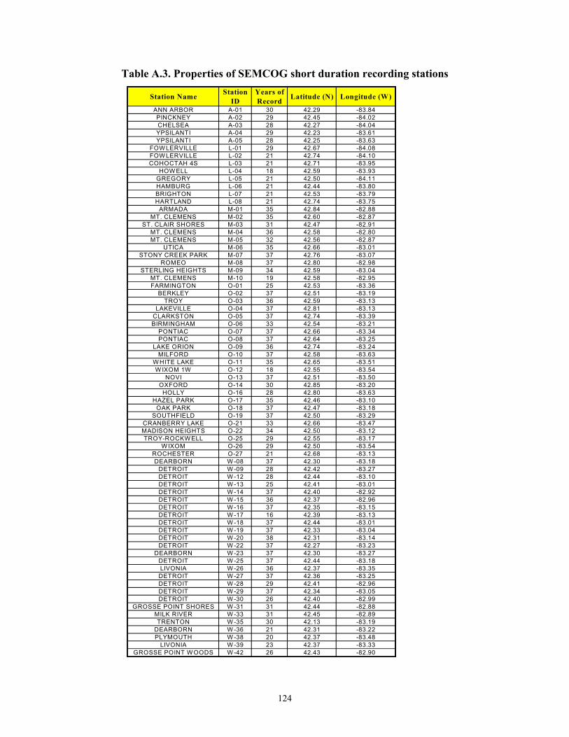
124

Table A.3. Properties of SEMCOG short duration recording stations

ANN ARBOR A-01 30 42.29 -83.84PINCKNEY A-02 29 42.45 -84.02CHELSEA A-03 28 42.27 -84.04YPSILANTI A-04 29 42.23 -83.61YPSILANTI A-05 28 42.25 -83.63

FOW LERVILLE L-01 29 42.67 -84.08FOW LERVILLE L-02 21 42.74 -84.10COHOCTAH 4S L-03 21 42.71 -83.95

HOW ELL L-04 18 42.59 -83.93GREGORY L-05 21 42.50 -84.11HAMBURG L-06 21 42.44 -83.80BRIGHTON L-07 21 42.53 -83.79HARTLAND L-08 21 42.74 -83.75

ARMADA M-01 35 42.84 -82.88MT. CLEMENS M-02 35 42.60 -82.87

ST. CLAIR SHORES M-03 31 42.47 -82.91MT. CLEMENS M-04 36 42.58 -82.80MT. CLEMENS M-05 32 42.56 -82.87

UTICA M-06 35 42.66 -83.01STONY CREEK PARK M-07 37 42.76 -83.07

ROMEO M-08 37 42.80 -82.98STERLING HEIGHTS M-09 34 42.59 -83.04

MT. CLEMENS M-10 19 42.58 -82.95FARMINGTON O-01 25 42.53 -83.36

BERKLEY O-02 37 42.51 -83.19TROY O-03 36 42.59 -83.13

LAKEVILLE O-04 37 42.81 -83.13CLARKSTON O-05 37 42.74 -83.39BIRMINGHAM O-06 33 42.54 -83.21

PONTIAC O-07 37 42.66 -83.34PONTIAC O-08 37 42.64 -83.25

LAKE ORION O-09 36 42.74 -83.24MILFORD O-10 37 42.58 -83.63

W HITE LAKE O-11 35 42.65 -83.51W IXOM 1W O-12 18 42.55 -83.54

NOVI O-13 37 42.51 -83.50OXFORD O-14 30 42.85 -83.20

HOLLY O-16 28 42.80 -83.63HAZEL PARK O-17 35 42.46 -83.10

OAK PARK O-18 37 42.47 -83.18SOUTHFIELD O-19 37 42.50 -83.29

CRANBERRY LAKE O-21 33 42.66 -83.47MADISON HEIGHTS O-22 34 42.50 -83.12TROY-ROCKW ELL O-25 29 42.55 -83.17

W IXOM O-26 29 42.50 -83.54ROCHESTER O-27 21 42.68 -83.13DEARBORN W -08 37 42.30 -83.18

DETROIT W -09 28 42.42 -83.27DETROIT W -12 28 42.44 -83.10DETROIT W -13 25 42.41 -83.01DETROIT W -14 37 42.40 -82.92DETROIT W -15 36 42.37 -82.96DETROIT W -16 37 42.35 -83.15DETROIT W -17 16 42.39 -83.13DETROIT W -18 37 42.44 -83.01DETROIT W -19 37 42.33 -83.04DETROIT W -20 38 42.31 -83.14DETROIT W -22 37 42.27 -83.23

DEARBORN W -23 37 42.30 -83.27DETROIT W -25 37 42.44 -83.18LIVONIA W -26 36 42.37 -83.35DETROIT W -27 37 42.36 -83.25DETROIT W -28 29 42.41 -82.96DETROIT W -29 37 42.34 -83.05DETROIT W -30 26 42.40 -82.99

GROSSE POINT SHORES W -31 31 42.44 -82.88MILK RIVER W -33 31 42.45 -82.89TRENTON W -35 30 42.13 -83.19

DEARBORN W -36 21 42.31 -83.22PLYMOUTH W -38 20 42.37 -83.48

LIVONIA W -39 23 42.37 -83.33GROSSE POINT W OODS W -42 26 42.43 -82.90

Station Name Station ID

Years of Record Latitude (N) Longitude (W)

125

Appendix B Recommended IDF Estimates

Figure B.1. NWS Climatic Zones

Table B.1. Recommended IDF Estimates for 10 Climatic Zones (values in inches)

Zone 1 Duration (min) 2-yr 5-yr 10-yr 25-yr 50-yr 100-yr

5 0.30 0.37 0.42 0.48 0.53 0.57 10 0.46 0.57 0.64 0.74 0.81 0.88 15 0.55 0.68 0.78 0.90 0.99 1.08 30 0.74 0.94 1.08 1.26 1.40 1.54

60 (1-hr) 1.02 1.30 1.53 1.83 2.07 2.31 120 (2-hr) 1.19 1.52 1.80 2.19 2.50 2.81 180 (3-hr) 1.31 1.68 1.98 2.23 2.56 2.89 360 (6-hr) 1.54 1.95 2.30 2.79 3.20 3.64 720 (12-hr) 1.82 2.29 2.69 3.24 3.70 4.20 1080 (18-hr) 1.98 2.49 2.91 3.51 4.01 4.53 1440 (24-hr) 2.38 2.97 3.47 4.19 4.79 5.43

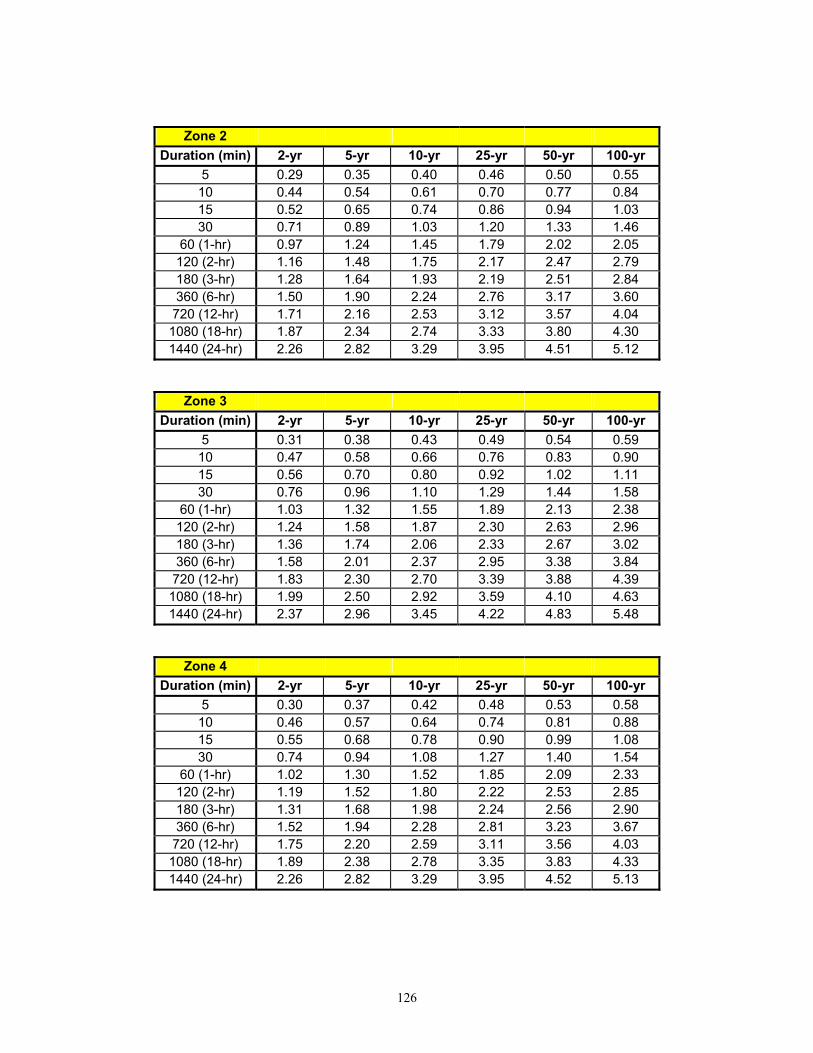
126

Zone 2 Duration (min) 2-yr 5-yr 10-yr 25-yr 50-yr 100-yr

5 0.29 0.35 0.40 0.46 0.50 0.55 10 0.44 0.54 0.61 0.70 0.77 0.84 15 0.52 0.65 0.74 0.86 0.94 1.03 30 0.71 0.89 1.03 1.20 1.33 1.46

60 (1-hr) 0.97 1.24 1.45 1.79 2.02 2.05 120 (2-hr) 1.16 1.48 1.75 2.17 2.47 2.79 180 (3-hr) 1.28 1.64 1.93 2.19 2.51 2.84 360 (6-hr) 1.50 1.90 2.24 2.76 3.17 3.60 720 (12-hr) 1.71 2.16 2.53 3.12 3.57 4.04 1080 (18-hr) 1.87 2.34 2.74 3.33 3.80 4.30 1440 (24-hr) 2.26 2.82 3.29 3.95 4.51 5.12

Zone 3 Duration (min) 2-yr 5-yr 10-yr 25-yr 50-yr 100-yr

5 0.31 0.38 0.43 0.49 0.54 0.59 10 0.47 0.58 0.66 0.76 0.83 0.90 15 0.56 0.70 0.80 0.92 1.02 1.11 30 0.76 0.96 1.10 1.29 1.44 1.58

60 (1-hr) 1.03 1.32 1.55 1.89 2.13 2.38 120 (2-hr) 1.24 1.58 1.87 2.30 2.63 2.96 180 (3-hr) 1.36 1.74 2.06 2.33 2.67 3.02 360 (6-hr) 1.58 2.01 2.37 2.95 3.38 3.84 720 (12-hr) 1.83 2.30 2.70 3.39 3.88 4.39 1080 (18-hr) 1.99 2.50 2.92 3.59 4.10 4.63 1440 (24-hr) 2.37 2.96 3.45 4.22 4.83 5.48

Zone 4 Duration (min) 2-yr 5-yr 10-yr 25-yr 50-yr 100-yr

5 0.30 0.37 0.42 0.48 0.53 0.58 10 0.46 0.57 0.64 0.74 0.81 0.88 15 0.55 0.68 0.78 0.90 0.99 1.08 30 0.74 0.94 1.08 1.27 1.40 1.54

60 (1-hr) 1.02 1.30 1.52 1.85 2.09 2.33 120 (2-hr) 1.19 1.52 1.80 2.22 2.53 2.85 180 (3-hr) 1.31 1.68 1.98 2.24 2.56 2.90 360 (6-hr) 1.52 1.94 2.28 2.81 3.23 3.67 720 (12-hr) 1.75 2.20 2.59 3.11 3.56 4.03 1080 (18-hr) 1.89 2.38 2.78 3.35 3.83 4.33 1440 (24-hr) 2.26 2.82 3.29 3.95 4.52 5.13

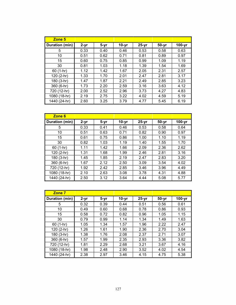
127

Zone 5 Duration (min) 2-yr 5-yr 10-yr 25-yr 50-yr 100-yr

5 0.33 0.40 0.46 0.53 0.58 0.63 10 0.51 0.62 0.71 0.81 0.89 0.97 15 0.60 0.75 0.85 0.99 1.09 1.19 30 0.81 1.03 1.18 1.39 1.54 1.69

60 (1-hr) 1.12 1.42 1.67 2.05 2.31 2.57 120 (2-hr) 1.33 1.70 2.01 2.47 2.81 3.17 180 (3-hr) 1.47 1.87 2.21 2.49 2.85 3.23 360 (6-hr) 1.73 2.20 2.59 3.16 3.63 4.12 720 (12-hr) 2.00 2.52 2.96 3.73 4.27 4.83 1080 (18-hr) 2.19 2.75 3.22 4.02 4.59 5.19 1440 (24-hr) 2.60 3.25 3.79 4.77 5.45 6.19

Zone 6 Duration (min) 2-yr 5-yr 10-yr 25-yr 50-yr 100-yr

5 0.33 0.41 0.46 0.53 0.58 0.64 10 0.51 0.63 0.71 0.82 0.90 0.97 15 0.61 0.75 0.86 1.00 1.10 1.19 30 0.82 1.03 1.19 1.40 1.55 1.70

60 (1-hr) 1.11 1.42 1.66 2.09 2.36 2.62 120 (2-hr) 1.31 1.68 1.99 2.46 2.81 3.16 180 (3-hr) 1.45 1.85 2.19 2.47 2.83 3.20 360 (6-hr) 1.67 2.12 2.50 3.09 3.54 4.02 720 (12-hr) 1.92 2.42 2.85 3.46 3.96 4.49 1080 (18-hr) 2.10 2.63 3.08 3.78 4.31 4.88 1440 (24-hr) 2.50 3.12 3.64 4.44 5.08 5.77

Zone 7 Duration (min) 2-yr 5-yr 10-yr 25-yr 50-yr 100-yr

5 0.32 0.39 0.44 0.51 0.56 0.61 10 0.49 0.60 0.68 0.78 0.86 0.93 15 0.58 0.72 0.82 0.96 1.05 1.15 30 0.79 0.99 1.14 1.34 1.49 1.63

60 (1-hr) 1.05 1.34 1.57 1.96 2.22 2.47 120 (2-hr) 1.26 1.61 1.90 2.36 2.70 3.04 180 (3-hr) 1.38 1.76 2.08 2.37 2.71 3.07 360 (6-hr) 1.57 1.99 2.35 2.93 3.36 3.82 720 (12-hr) 1.81 2.29 2.68 3.21 3.67 4.16 1080 (18-hr) 1.98 2.48 2.90 3.52 4.02 4.54 1440 (24-hr) 2.38 2.97 3.46 4.15 4.75 5.38

128

Zone 8 Duration (min) 2-yr 5-yr 10-yr 25-yr 50-yr 100-yr

5 0.35 0.42 0.48 0.55 0.61 0.66 10 0.53 0.65 0.74 0.85 0.93 1.01 15 0.63 0.78 0.89 1.03 1.14 1.24 30 0.85 1.07 1.24 1.45 1.61 1.77

60 (1-hr) 1.16 1.48 1.74 2.10 2.37 2.64 120 (2-hr) 1.38 1.76 2.08 2.52 2.87 3.23 180 (3-hr) 1.52 1.94 2.29 2.59 2.96 3.35 360 (6-hr) 1.79 2.27 2.68 3.24 3.72 4.22 720 (12-hr) 2.07 2.61 3.06 3.74 4.27 4.84 1080 (18-hr) 2.25 2.83 3.31 4.06 4.64 5.24 1440 (24-hr) 2.69 3.36 3.92 4.82 5.51 6.25

Zone 9 Duration (min) 2-yr 5-yr 10-yr 25-yr 50-yr 100-yr

5 0.34 0.42 0.48 0.55 0.60 0.66 10 0.53 0.65 0.73 0.84 0.92 1.00 15 0.63 0.78 0.89 1.03 1.13 1.23 30 0.84 1.07 1.23 1.44 1.60 1.75

60 (1-hr) 1.16 1.48 1.74 2.08 2.35 2.62 120 (2-hr) 1.36 1.74 2.05 2.49 2.84 3.20 180 (3-hr) 1.49 1.91 2.26 2.55 2.92 3.30 360 (6-hr) 1.72 2.19 2.58 3.14 3.61 4.10 720 (12-hr) 1.97 2.48 2.92 3.53 4.04 4.57 1080 (18-hr) 2.14 2.68 3.14 3.81 4.35 4.91 1440 (24-hr) 2.56 3.20 3.73 4.50 5.15 5.85

Zone 10 Duration (min) 2-yr 5-yr 10-yr 25-yr 50-yr 100-yr

5 0.33 0.40 0.45 0.52 0.57 0.62 10 0.50 0.62 0.70 0.80 0.88 0.96 15 0.60 0.74 0.84 0.98 1.08 1.17 30 0.81 1.02 1.17 1.37 1.52 1.67

60 (1-hr) 1.11 1.41 1.66 1.97 2.23 2.48 120 (2-hr) 1.29 1.66 1.96 2.36 2.69 3.03 180 (3-hr) 1.42 1.82 2.15 2.43 2.78 3.14 360 (6-hr) 1.63 2.08 2.45 2.97 3.40 3.87 720 (12-hr) 1.86 2.34 2.75 3.39 3.88 4.39 1080 (18-hr) 2.02 2.54 2.97 3.60 4.11 4.65 1440 (24-hr) 2.42 3.02 3.52 4.24 4.85 5.50

129

Appendix C Rainfall Intensity - Duration Tables for MDOT Road

Design Manual.

Figure C.1. Ten National Weather Service (NWS) zones located in Michigan and used as rainfall frequency zones.

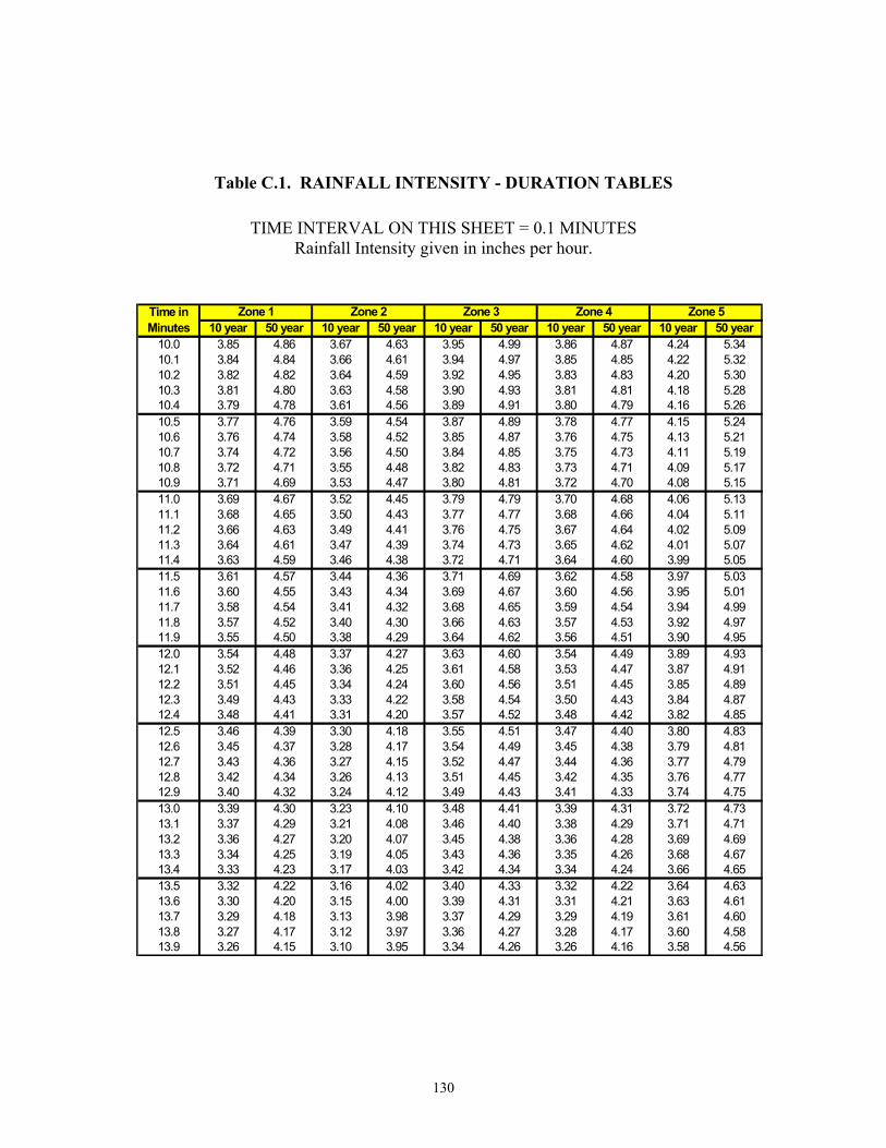
130

Table C.1. RAINFALL INTENSITY - DURATION TABLES

TIME INTERVAL ON THIS SHEET = 0.1 MINUTES Rainfall Intensity given in inches per hour.

10 year 50 year 10 year 50 year 10 year 50 year 10 year 50 year 10 year 50 year10.0 3.85 4.86 3.67 4.63 3.95 4.99 3.86 4.87 4.24 5.3410.1 3.84 4.84 3.66 4.61 3.94 4.97 3.85 4.85 4.22 5.3210.2 3.82 4.82 3.64 4.59 3.92 4.95 3.83 4.83 4.20 5.3010.3 3.81 4.80 3.63 4.58 3.90 4.93 3.81 4.81 4.18 5.2810.4 3.79 4.78 3.61 4.56 3.89 4.91 3.80 4.79 4.16 5.2610.5 3.77 4.76 3.59 4.54 3.87 4.89 3.78 4.77 4.15 5.2410.6 3.76 4.74 3.58 4.52 3.85 4.87 3.76 4.75 4.13 5.2110.7 3.74 4.72 3.56 4.50 3.84 4.85 3.75 4.73 4.11 5.1910.8 3.72 4.71 3.55 4.48 3.82 4.83 3.73 4.71 4.09 5.1710.9 3.71 4.69 3.53 4.47 3.80 4.81 3.72 4.70 4.08 5.1511.0 3.69 4.67 3.52 4.45 3.79 4.79 3.70 4.68 4.06 5.1311.1 3.68 4.65 3.50 4.43 3.77 4.77 3.68 4.66 4.04 5.1111.2 3.66 4.63 3.49 4.41 3.76 4.75 3.67 4.64 4.02 5.0911.3 3.64 4.61 3.47 4.39 3.74 4.73 3.65 4.62 4.01 5.0711.4 3.63 4.59 3.46 4.38 3.72 4.71 3.64 4.60 3.99 5.0511.5 3.61 4.57 3.44 4.36 3.71 4.69 3.62 4.58 3.97 5.0311.6 3.60 4.55 3.43 4.34 3.69 4.67 3.60 4.56 3.95 5.0111.7 3.58 4.54 3.41 4.32 3.68 4.65 3.59 4.54 3.94 4.9911.8 3.57 4.52 3.40 4.30 3.66 4.63 3.57 4.53 3.92 4.9711.9 3.55 4.50 3.38 4.29 3.64 4.62 3.56 4.51 3.90 4.9512.0 3.54 4.48 3.37 4.27 3.63 4.60 3.54 4.49 3.89 4.9312.1 3.52 4.46 3.36 4.25 3.61 4.58 3.53 4.47 3.87 4.9112.2 3.51 4.45 3.34 4.24 3.60 4.56 3.51 4.45 3.85 4.8912.3 3.49 4.43 3.33 4.22 3.58 4.54 3.50 4.43 3.84 4.8712.4 3.48 4.41 3.31 4.20 3.57 4.52 3.48 4.42 3.82 4.8512.5 3.46 4.39 3.30 4.18 3.55 4.51 3.47 4.40 3.80 4.8312.6 3.45 4.37 3.28 4.17 3.54 4.49 3.45 4.38 3.79 4.8112.7 3.43 4.36 3.27 4.15 3.52 4.47 3.44 4.36 3.77 4.7912.8 3.42 4.34 3.26 4.13 3.51 4.45 3.42 4.35 3.76 4.7712.9 3.40 4.32 3.24 4.12 3.49 4.43 3.41 4.33 3.74 4.7513.0 3.39 4.30 3.23 4.10 3.48 4.41 3.39 4.31 3.72 4.7313.1 3.37 4.29 3.21 4.08 3.46 4.40 3.38 4.29 3.71 4.7113.2 3.36 4.27 3.20 4.07 3.45 4.38 3.36 4.28 3.69 4.6913.3 3.34 4.25 3.19 4.05 3.43 4.36 3.35 4.26 3.68 4.6713.4 3.33 4.23 3.17 4.03 3.42 4.34 3.34 4.24 3.66 4.6513.5 3.32 4.22 3.16 4.02 3.40 4.33 3.32 4.22 3.64 4.6313.6 3.30 4.20 3.15 4.00 3.39 4.31 3.31 4.21 3.63 4.6113.7 3.29 4.18 3.13 3.98 3.37 4.29 3.29 4.19 3.61 4.6013.8 3.27 4.17 3.12 3.97 3.36 4.27 3.28 4.17 3.60 4.5813.9 3.26 4.15 3.10 3.95 3.34 4.26 3.26 4.16 3.58 4.56

Zone 4Time in Minutes

Zone 1 Zone 2 Zone 3 Zone 5

131

Table C.1 (continued). RAINFALL INTENSITY - DURATION TABLES

TIME INTERVAL ON THIS SHEET = 0.1 MINUTES Rainfall Intensity given in inches per hour.

10 year 50 year 10 year 50 year 10 year 50 year 10 year 50 year 10 year 50 year14.0 3.24 4.13 3.09 3.94 3.33 4.24 3.25 4.14 3.57 4.5414.1 3.23 4.11 3.08 3.92 3.32 4.22 3.24 4.12 3.55 4.5214.2 3.22 4.10 3.06 3.90 3.30 4.20 3.22 4.10 3.54 4.5014.3 3.20 4.08 3.05 3.89 3.29 4.19 3.21 4.09 3.52 4.4914.4 3.19 4.06 3.04 3.87 3.27 4.17 3.19 4.07 3.51 4.4714.5 3.18 4.05 3.03 3.86 3.26 4.15 3.18 4.05 3.49 4.4514.6 3.16 4.03 3.01 3.84 3.24 4.14 3.17 4.04 3.47 4.4314.7 3.15 4.02 3.00 3.83 3.23 4.12 3.15 4.02 3.46 4.4114.8 3.13 4.00 2.99 3.81 3.22 4.10 3.14 4.01 3.45 4.3914.9 3.12 3.98 2.97 3.79 3.20 4.09 3.13 3.99 3.43 4.3815.0 3.11 3.97 2.96 3.78 3.19 4.07 3.11 3.97 3.42 4.3615.1 3.10 3.96 2.95 3.77 3.18 4.06 3.11 3.96 3.41 4.3515.2 3.09 3.95 2.95 3.76 3.17 4.05 3.10 3.95 3.40 4.3415.3 3.09 3.94 2.94 3.75 3.17 4.04 3.09 3.95 3.39 4.3315.4 3.08 3.93 2.93 3.74 3.16 4.03 3.08 3.94 3.38 4.3215.5 3.07 3.92 2.92 3.74 3.15 4.02 3.08 3.93 3.37 4.3115.6 3.06 3.91 2.92 3.73 3.14 4.01 3.07 3.92 3.37 4.3015.7 3.06 3.90 2.91 3.72 3.14 4.00 3.06 3.91 3.36 4.2915.8 3.05 3.89 2.90 3.71 3.13 4.00 3.05 3.90 3.35 4.2815.9 3.04 3.89 2.90 3.70 3.12 3.99 3.05 3.89 3.34 4.2716.0 3.03 3.88 2.89 3.69 3.11 3.98 3.04 3.88 3.33 4.2616.1 3.03 3.87 2.88 3.68 3.10 3.97 3.03 3.87 3.33 4.2516.2 3.02 3.86 2.88 3.68 3.10 3.96 3.02 3.86 3.32 4.2416.3 3.01 3.85 2.87 3.67 3.09 3.95 3.02 3.86 3.31 4.2316.4 3.00 3.84 2.86 3.66 3.08 3.94 3.01 3.85 3.30 4.2216.5 3.00 3.83 2.85 3.65 3.07 3.93 3.00 3.84 3.29 4.2116.6 2.99 3.82 2.85 3.64 3.07 3.92 2.99 3.83 3.28 4.2016.7 2.98 3.81 2.84 3.63 3.06 3.91 2.99 3.82 3.28 4.1916.8 2.97 3.81 2.83 3.62 3.05 3.90 2.98 3.81 3.27 4.1816.9 2.97 3.80 2.83 3.62 3.04 3.89 2.97 3.80 3.26 4.1717.0 2.96 3.79 2.82 3.61 3.04 3.89 2.96 3.79 3.25 4.1617.1 2.95 3.78 2.81 3.60 3.03 3.88 2.96 3.78 3.24 4.1517.2 2.95 3.77 2.81 3.59 3.02 3.87 2.95 3.78 3.24 4.1417.3 2.94 3.76 2.80 3.58 3.01 3.86 2.94 3.77 3.23 4.1317.4 2.93 3.75 2.79 3.57 3.01 3.85 2.94 3.76 3.22 4.1217.5 2.92 3.74 2.79 3.57 3.00 3.84 2.93 3.75 3.21 4.1117.6 2.92 3.74 2.78 3.56 2.99 3.83 2.92 3.74 3.21 4.1017.7 2.91 3.73 2.77 3.55 2.99 3.82 2.91 3.73 3.20 4.1017.8 2.90 3.72 2.76 3.54 2.98 3.81 2.91 3.72 3.19 4.0917.9 2.90 3.71 2.76 3.53 2.97 3.81 2.90 3.72 3.18 4.08

Zone 4Time in Minutes

Zone 1 Zone 2 Zone 3 Zone 5

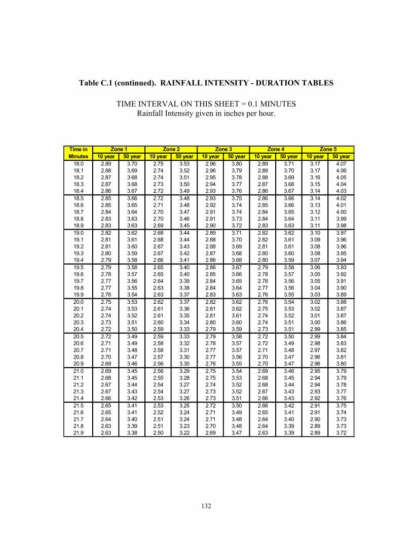
132

Table C.1 (continued). RAINFALL INTENSITY - DURATION TABLES

TIME INTERVAL ON THIS SHEET = 0.1 MINUTES Rainfall Intensity given in inches per hour.

10 year 50 year 10 year 50 year 10 year 50 year 10 year 50 year 10 year 50 year18.0 2.89 3.70 2.75 3.53 2.96 3.80 2.89 3.71 3.17 4.0718.1 2.88 3.69 2.74 3.52 2.96 3.79 2.89 3.70 3.17 4.0618.2 2.87 3.68 2.74 3.51 2.95 3.78 2.88 3.69 3.16 4.0518.3 2.87 3.68 2.73 3.50 2.94 3.77 2.87 3.68 3.15 4.0418.4 2.86 3.67 2.72 3.49 2.93 3.76 2.86 3.67 3.14 4.0318.5 2.85 3.66 2.72 3.48 2.93 3.75 2.86 3.66 3.14 4.0218.6 2.85 3.65 2.71 3.48 2.92 3.74 2.85 3.66 3.13 4.0118.7 2.84 3.64 2.70 3.47 2.91 3.74 2.84 3.65 3.12 4.0018.8 2.83 3.63 2.70 3.46 2.91 3.73 2.84 3.64 3.11 3.9918.9 2.83 3.63 2.69 3.45 2.90 3.72 2.83 3.63 3.11 3.9819.0 2.82 3.62 2.68 3.44 2.89 3.71 2.82 3.62 3.10 3.9719.1 2.81 3.61 2.68 3.44 2.88 3.70 2.82 3.61 3.09 3.9619.2 2.81 3.60 2.67 3.43 2.88 3.69 2.81 3.61 3.08 3.9619.3 2.80 3.59 2.67 3.42 2.87 3.68 2.80 3.60 3.08 3.9519.4 2.79 3.58 2.66 3.41 2.86 3.68 2.80 3.59 3.07 3.9419.5 2.79 3.58 2.65 3.40 2.86 3.67 2.79 3.58 3.06 3.9319.6 2.78 3.57 2.65 3.40 2.85 3.66 2.78 3.57 3.05 3.9219.7 2.77 3.56 2.64 3.39 2.84 3.65 2.78 3.56 3.05 3.9119.8 2.77 3.55 2.63 3.38 2.84 3.64 2.77 3.56 3.04 3.9019.9 2.76 3.54 2.63 3.37 2.83 3.63 2.76 3.55 3.03 3.8920.0 2.75 3.53 2.62 3.37 2.82 3.62 2.76 3.54 3.02 3.8820.1 2.74 3.53 2.61 3.36 2.81 3.62 2.75 3.53 3.02 3.8720.2 2.74 3.52 2.61 3.35 2.81 3.61 2.74 3.52 3.01 3.8720.3 2.73 3.51 2.60 3.34 2.80 3.60 2.74 3.51 3.00 3.8620.4 2.72 3.50 2.59 3.33 2.79 3.59 2.73 3.51 2.99 3.8520.5 2.72 3.49 2.59 3.33 2.79 3.58 2.72 3.50 2.99 3.8420.6 2.71 3.49 2.58 3.32 2.78 3.57 2.72 3.49 2.98 3.8320.7 2.71 3.48 2.58 3.31 2.77 3.57 2.71 3.48 2.97 3.8220.8 2.70 3.47 2.57 3.30 2.77 3.56 2.70 3.47 2.96 3.8120.9 2.69 3.46 2.56 3.30 2.76 3.55 2.70 3.47 2.96 3.8021.0 2.69 3.45 2.56 3.29 2.75 3.54 2.69 3.46 2.95 3.7921.1 2.68 3.45 2.55 3.28 2.75 3.53 2.68 3.45 2.94 3.7921.2 2.67 3.44 2.54 3.27 2.74 3.52 2.68 3.44 2.94 3.7821.3 2.67 3.43 2.54 3.27 2.73 3.52 2.67 3.43 2.93 3.7721.4 2.66 3.42 2.53 3.26 2.73 3.51 2.66 3.43 2.92 3.7621.5 2.65 3.41 2.53 3.25 2.72 3.50 2.66 3.42 2.91 3.7521.6 2.65 3.41 2.52 3.24 2.71 3.49 2.65 3.41 2.91 3.7421.7 2.64 3.40 2.51 3.24 2.71 3.48 2.64 3.40 2.90 3.7321.8 2.63 3.39 2.51 3.23 2.70 3.48 2.64 3.39 2.89 3.7321.9 2.63 3.38 2.50 3.22 2.69 3.47 2.63 3.39 2.89 3.72

Time in Minutes

Zone 1 Zone 2 Zone 3 Zone 4 Zone 5

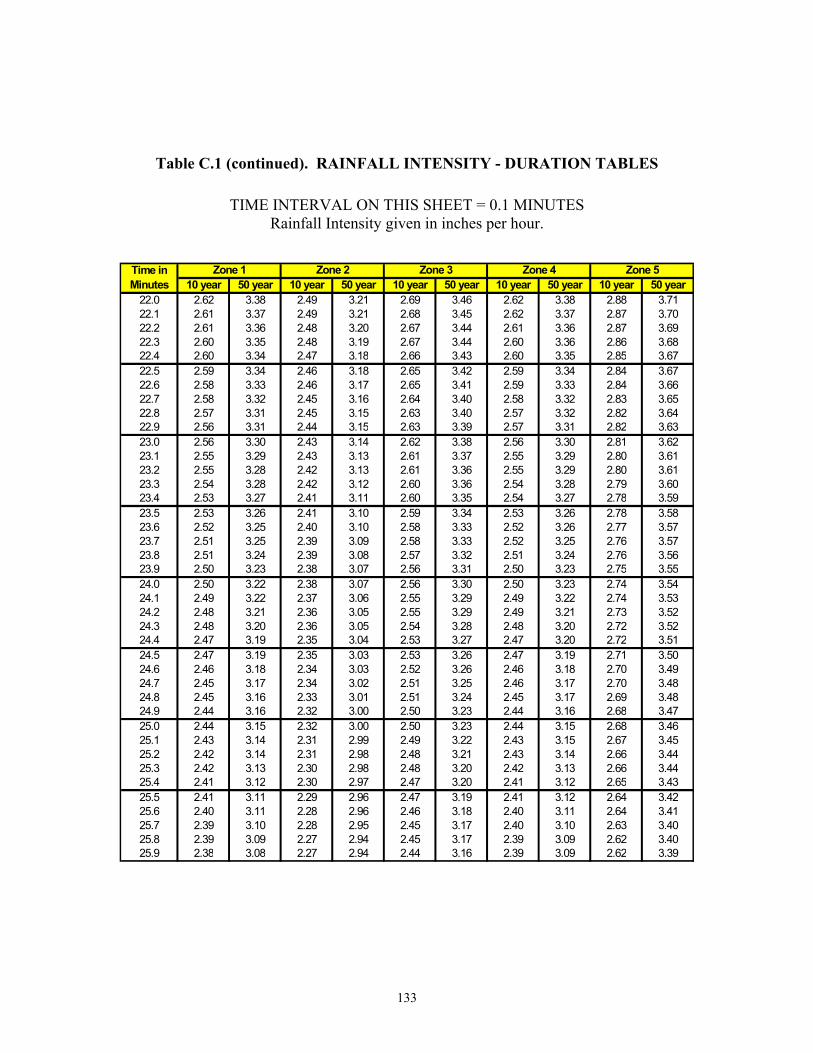
133

Table C.1 (continued). RAINFALL INTENSITY - DURATION TABLES

TIME INTERVAL ON THIS SHEET = 0.1 MINUTES Rainfall Intensity given in inches per hour.

10 year 50 year 10 year 50 year 10 year 50 year 10 year 50 year 10 year 50 year22.0 2.62 3.38 2.49 3.21 2.69 3.46 2.62 3.38 2.88 3.7122.1 2.61 3.37 2.49 3.21 2.68 3.45 2.62 3.37 2.87 3.7022.2 2.61 3.36 2.48 3.20 2.67 3.44 2.61 3.36 2.87 3.6922.3 2.60 3.35 2.48 3.19 2.67 3.44 2.60 3.36 2.86 3.6822.4 2.60 3.34 2.47 3.18 2.66 3.43 2.60 3.35 2.85 3.6722.5 2.59 3.34 2.46 3.18 2.65 3.42 2.59 3.34 2.84 3.6722.6 2.58 3.33 2.46 3.17 2.65 3.41 2.59 3.33 2.84 3.6622.7 2.58 3.32 2.45 3.16 2.64 3.40 2.58 3.32 2.83 3.6522.8 2.57 3.31 2.45 3.15 2.63 3.40 2.57 3.32 2.82 3.6422.9 2.56 3.31 2.44 3.15 2.63 3.39 2.57 3.31 2.82 3.6323.0 2.56 3.30 2.43 3.14 2.62 3.38 2.56 3.30 2.81 3.6223.1 2.55 3.29 2.43 3.13 2.61 3.37 2.55 3.29 2.80 3.6123.2 2.55 3.28 2.42 3.13 2.61 3.36 2.55 3.29 2.80 3.6123.3 2.54 3.28 2.42 3.12 2.60 3.36 2.54 3.28 2.79 3.6023.4 2.53 3.27 2.41 3.11 2.60 3.35 2.54 3.27 2.78 3.5923.5 2.53 3.26 2.41 3.10 2.59 3.34 2.53 3.26 2.78 3.5823.6 2.52 3.25 2.40 3.10 2.58 3.33 2.52 3.26 2.77 3.5723.7 2.51 3.25 2.39 3.09 2.58 3.33 2.52 3.25 2.76 3.5723.8 2.51 3.24 2.39 3.08 2.57 3.32 2.51 3.24 2.76 3.5623.9 2.50 3.23 2.38 3.07 2.56 3.31 2.50 3.23 2.75 3.5524.0 2.50 3.22 2.38 3.07 2.56 3.30 2.50 3.23 2.74 3.5424.1 2.49 3.22 2.37 3.06 2.55 3.29 2.49 3.22 2.74 3.5324.2 2.48 3.21 2.36 3.05 2.55 3.29 2.49 3.21 2.73 3.5224.3 2.48 3.20 2.36 3.05 2.54 3.28 2.48 3.20 2.72 3.5224.4 2.47 3.19 2.35 3.04 2.53 3.27 2.47 3.20 2.72 3.5124.5 2.47 3.19 2.35 3.03 2.53 3.26 2.47 3.19 2.71 3.5024.6 2.46 3.18 2.34 3.03 2.52 3.26 2.46 3.18 2.70 3.4924.7 2.45 3.17 2.34 3.02 2.51 3.25 2.46 3.17 2.70 3.4824.8 2.45 3.16 2.33 3.01 2.51 3.24 2.45 3.17 2.69 3.4824.9 2.44 3.16 2.32 3.00 2.50 3.23 2.44 3.16 2.68 3.4725.0 2.44 3.15 2.32 3.00 2.50 3.23 2.44 3.15 2.68 3.4625.1 2.43 3.14 2.31 2.99 2.49 3.22 2.43 3.15 2.67 3.4525.2 2.42 3.14 2.31 2.98 2.48 3.21 2.43 3.14 2.66 3.4425.3 2.42 3.13 2.30 2.98 2.48 3.20 2.42 3.13 2.66 3.4425.4 2.41 3.12 2.30 2.97 2.47 3.20 2.41 3.12 2.65 3.4325.5 2.41 3.11 2.29 2.96 2.47 3.19 2.41 3.12 2.64 3.4225.6 2.40 3.11 2.28 2.96 2.46 3.18 2.40 3.11 2.64 3.4125.7 2.39 3.10 2.28 2.95 2.45 3.17 2.40 3.10 2.63 3.4025.8 2.39 3.09 2.27 2.94 2.45 3.17 2.39 3.09 2.62 3.4025.9 2.38 3.08 2.27 2.94 2.44 3.16 2.39 3.09 2.62 3.39

Zone 4Time in Minutes

Zone 1 Zone 2 Zone 3 Zone 5

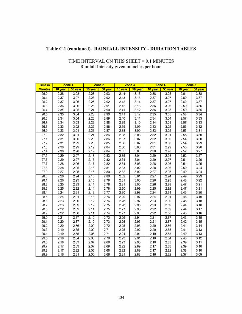
134

Table C.1 (continued). RAINFALL INTENSITY - DURATION TABLES

TIME INTERVAL ON THIS SHEET = 0.1 MINUTES Rainfall Intensity given in inches per hour.

10 year 50 year 10 year 50 year 10 year 50 year 10 year 50 year 10 year 50 year26.0 2.38 3.08 2.26 2.93 2.44 3.15 2.38 3.08 2.61 3.3826.1 2.37 3.07 2.26 2.92 2.43 3.15 2.37 3.07 2.60 3.3726.2 2.37 3.06 2.25 2.92 2.42 3.14 2.37 3.07 2.60 3.3726.3 2.36 3.06 2.25 2.91 2.42 3.13 2.36 3.06 2.59 3.3626.4 2.35 3.05 2.24 2.90 2.41 3.12 2.36 3.05 2.59 3.3526.5 2.35 3.04 2.23 2.90 2.41 3.12 2.35 3.05 2.58 3.3426.6 2.34 3.04 2.23 2.89 2.40 3.11 2.34 3.04 2.57 3.3326.7 2.34 3.03 2.22 2.88 2.39 3.10 2.34 3.03 2.57 3.3326.8 2.33 3.02 2.22 2.88 2.39 3.09 2.33 3.02 2.56 3.3226.9 2.33 3.01 2.21 2.87 2.38 3.09 2.33 3.02 2.55 3.3127.0 2.32 3.01 2.21 2.86 2.38 3.08 2.32 3.01 2.55 3.3027.1 2.31 3.00 2.20 2.86 2.37 3.07 2.32 3.00 2.54 3.3027.2 2.31 2.99 2.20 2.85 2.36 3.07 2.31 3.00 2.54 3.2927.3 2.30 2.99 2.19 2.84 2.36 3.06 2.31 2.99 2.53 3.2827.4 2.30 2.98 2.19 2.84 2.35 3.05 2.30 2.98 2.52 3.2727.5 2.29 2.97 2.18 2.83 2.35 3.04 2.29 2.98 2.52 3.2727.6 2.29 2.97 2.18 2.82 2.34 3.04 2.29 2.97 2.51 3.2627.7 2.28 2.96 2.17 2.82 2.34 3.03 2.28 2.96 2.51 3.2527.8 2.28 2.95 2.16 2.81 2.33 3.02 2.28 2.96 2.50 3.2427.9 2.27 2.95 2.16 2.80 2.32 3.02 2.27 2.95 2.49 3.2428.0 2.26 2.94 2.15 2.80 2.32 3.01 2.27 2.94 2.49 3.2328.1 2.26 2.93 2.15 2.79 2.31 3.00 2.26 2.93 2.48 3.2228.2 2.25 2.93 2.14 2.78 2.31 3.00 2.26 2.93 2.47 3.2128.3 2.25 2.92 2.14 2.78 2.30 2.99 2.25 2.92 2.47 3.2128.4 2.24 2.91 2.13 2.77 2.30 2.98 2.24 2.91 2.46 3.2028.5 2.24 2.91 2.13 2.76 2.29 2.97 2.24 2.91 2.46 3.1928.6 2.23 2.90 2.12 2.76 2.28 2.97 2.23 2.90 2.45 3.1828.7 2.23 2.89 2.12 2.75 2.28 2.96 2.23 2.89 2.44 3.1828.8 2.22 2.89 2.11 2.75 2.27 2.95 2.22 2.89 2.44 3.1728.9 2.22 2.88 2.11 2.74 2.27 2.95 2.22 2.88 2.43 3.1629.0 2.21 2.87 2.10 2.73 2.26 2.94 2.21 2.87 2.43 3.1529.1 2.20 2.87 2.10 2.73 2.26 2.93 2.21 2.87 2.42 3.1529.2 2.20 2.86 2.09 2.72 2.25 2.93 2.20 2.86 2.41 3.1429.3 2.19 2.85 2.09 2.71 2.25 2.92 2.20 2.85 2.41 3.1329.4 2.19 2.85 2.08 2.71 2.24 2.91 2.19 2.85 2.40 3.1329.5 2.18 2.84 2.08 2.70 2.23 2.91 2.18 2.84 2.40 3.1229.6 2.18 2.83 2.07 2.69 2.23 2.90 2.18 2.83 2.39 3.1129.7 2.17 2.83 2.07 2.69 2.22 2.89 2.17 2.83 2.39 3.1029.8 2.17 2.82 2.06 2.68 2.22 2.89 2.17 2.82 2.38 3.1029.9 2.16 2.81 2.06 2.68 2.21 2.88 2.16 2.82 2.37 3.09

Time in Minutes

Zone 1 Zone 2 Zone 3 Zone 4 Zone 5

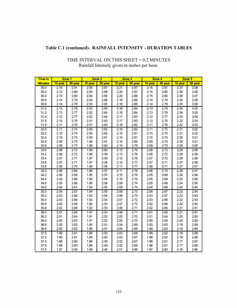
135

Table C.1 (continued). RAINFALL INTENSITY - DURATION TABLES

TIME INTERVAL ON THIS SHEET = 0.2 MINUTES Rainfall Intensity given in inches per hour.

10 year 50 year 10 year 50 year 10 year 50 year 10 year 50 year 10 year 50 year30.0 2.16 2.81 2.05 2.67 2.21 2.87 2.16 2.81 2.37 3.0830.2 2.15 2.80 2.05 2.66 2.20 2.87 2.15 2.80 2.36 3.0830.4 2.15 2.80 2.04 2.66 2.20 2.86 2.15 2.80 2.36 3.0730.6 2.14 2.79 2.04 2.66 2.19 2.86 2.14 2.79 2.35 3.0630.8 2.14 2.78 2.03 2.65 2.19 2.85 2.14 2.79 2.35 3.0631.0 2.13 2.78 2.03 2.65 2.18 2.84 2.13 2.78 2.34 3.0531.2 2.13 2.77 2.02 2.64 2.18 2.84 2.13 2.78 2.34 3.0531.4 2.12 2.77 2.02 2.64 2.17 2.83 2.12 2.77 2.33 3.0431.6 2.12 2.76 2.01 2.63 2.17 2.83 2.12 2.76 2.32 3.0431.8 2.11 2.76 2.01 2.63 2.16 2.82 2.11 2.76 2.32 3.0332.0 2.11 2.75 2.00 2.62 2.16 2.82 2.11 2.75 2.31 3.0232.2 2.10 2.74 2.00 2.62 2.15 2.81 2.10 2.75 2.31 3.0232.4 2.10 2.74 2.00 2.61 2.15 2.81 2.10 2.74 2.30 3.0132.6 2.09 2.73 1.99 2.61 2.14 2.80 2.09 2.74 2.30 3.0132.8 2.09 2.73 1.99 2.60 2.14 2.79 2.09 2.73 2.29 3.0033.0 2.08 2.72 1.98 2.60 2.13 2.79 2.08 2.73 2.29 2.9933.2 2.08 2.72 1.98 2.59 2.13 2.78 2.08 2.72 2.28 2.9933.4 2.07 2.71 1.97 2.59 2.12 2.78 2.07 2.72 2.28 2.9833.6 2.07 2.71 1.97 2.58 2.12 2.77 2.07 2.71 2.27 2.9833.8 2.06 2.70 1.96 2.58 2.11 2.77 2.06 2.71 2.27 2.9734.0 2.06 2.69 1.96 2.57 2.11 2.76 2.06 2.70 2.26 2.9734.2 2.06 2.69 1.95 2.57 2.10 2.76 2.05 2.69 2.26 2.9634.4 2.05 2.68 1.95 2.56 2.10 2.75 2.05 2.69 2.25 2.9534.6 2.05 2.68 1.95 2.56 2.09 2.74 2.05 2.68 2.24 2.9534.8 2.04 2.67 1.94 2.55 2.09 2.74 2.04 2.68 2.24 2.9435.0 2.04 2.67 1.94 2.55 2.08 2.73 2.04 2.67 2.23 2.9435.2 2.03 2.66 1.93 2.54 2.08 2.73 2.03 2.67 2.23 2.9335.4 2.03 2.66 1.93 2.54 2.07 2.72 2.03 2.66 2.22 2.9335.6 2.02 2.65 1.92 2.53 2.07 2.72 2.02 2.66 2.22 2.9235.8 2.02 2.65 1.92 2.53 2.06 2.71 2.02 2.65 2.21 2.9136.0 2.01 2.64 1.91 2.53 2.06 2.71 2.01 2.65 2.21 2.9136.2 2.01 2.64 1.91 2.52 2.05 2.70 2.01 2.64 2.20 2.9036.4 2.00 2.63 1.91 2.52 2.05 2.70 2.00 2.64 2.20 2.9036.6 2.00 2.62 1.90 2.51 2.04 2.69 2.00 2.63 2.19 2.8936.8 2.00 2.62 1.90 2.51 2.04 2.69 1.99 2.63 2.19 2.8937.0 1.99 2.61 1.89 2.50 2.03 2.68 1.99 2.62 2.18 2.8837.2 1.99 2.61 1.89 2.50 2.03 2.67 1.98 2.62 2.18 2.8837.4 1.98 2.60 1.88 2.49 2.02 2.67 1.98 2.61 2.17 2.8737.6 1.98 2.60 1.88 2.49 2.02 2.66 1.98 2.61 2.17 2.8637.8 1.97 2.59 1.88 2.48 2.01 2.66 1.97 2.60 2.16 2.86

Time in Minutes

Zone 1 Zone 2 Zone 3 Zone 4 Zone 5

136

Table C.1 (continued). RAINFALL INTENSITY - DURATION TABLES

TIME INTERVAL ON THIS SHEET = 0.5 MINUTES Rainfall Intensity given in inches per hour.

10 year 50 year 10 year 50 year 10 year 50 year 10 year 50 year 10 year 50 year38.0 1.97 2.59 1.87 2.48 2.01 2.65 1.97 2.60 2.16 2.8538.5 1.96 2.57 1.86 2.47 2.00 2.64 1.95 2.58 2.15 2.8439.0 1.95 2.56 1.85 2.46 1.98 2.63 1.94 2.57 2.13 2.8339.5 1.93 2.55 1.84 2.44 1.97 2.61 1.93 2.56 2.12 2.8140.0 1.92 2.54 1.83 2.43 1.96 2.60 1.92 2.54 2.11 2.8040.5 1.91 2.52 1.82 2.42 1.95 2.59 1.91 2.53 2.10 2.7941.0 1.90 2.51 1.81 2.41 1.94 2.58 1.90 2.52 2.08 2.7741.5 1.89 2.50 1.80 2.40 1.93 2.56 1.89 2.51 2.07 2.7642.0 1.88 2.48 1.79 2.39 1.92 2.55 1.88 2.49 2.06 2.7542.5 1.87 2.47 1.78 2.38 1.90 2.54 1.87 2.48 2.05 2.7343.0 1.86 2.46 1.77 2.37 1.89 2.53 1.85 2.47 2.04 2.7243.5 1.85 2.45 1.76 2.36 1.88 2.51 1.84 2.46 2.02 2.7144.0 1.84 2.43 1.75 2.34 1.87 2.50 1.83 2.45 2.01 2.6944.5 1.83 2.42 1.74 2.33 1.86 2.49 1.82 2.43 2.00 2.6845.0 1.82 2.41 1.73 2.32 1.85 2.48 1.81 2.42 1.99 2.6745.5 1.81 2.40 1.72 2.31 1.84 2.46 1.80 2.41 1.98 2.6546.0 1.80 2.39 1.71 2.30 1.83 2.45 1.79 2.40 1.97 2.6446.5 1.79 2.37 1.70 2.29 1.82 2.44 1.78 2.39 1.95 2.6347.0 1.78 2.36 1.69 2.28 1.80 2.43 1.77 2.37 1.94 2.6247.5 1.77 2.35 1.68 2.27 1.79 2.42 1.76 2.36 1.93 2.6048.0 1.76 2.34 1.67 2.26 1.78 2.40 1.75 2.35 1.92 2.5948.5 1.75 2.33 1.66 2.25 1.77 2.39 1.74 2.34 1.91 2.5849.0 1.74 2.31 1.65 2.24 1.76 2.38 1.73 2.33 1.90 2.5749.5 1.73 2.30 1.64 2.23 1.75 2.37 1.72 2.32 1.89 2.5550.0 1.72 2.29 1.63 2.22 1.74 2.36 1.71 2.31 1.88 2.5450.5 1.71 2.28 1.62 2.21 1.73 2.34 1.70 2.29 1.87 2.5351.0 1.70 2.27 1.61 2.20 1.72 2.33 1.69 2.28 1.86 2.5251.5 1.69 2.26 1.60 2.19 1.71 2.32 1.68 2.27 1.84 2.5152.0 1.68 2.24 1.59 2.18 1.70 2.31 1.67 2.26 1.83 2.4952.5 1.67 2.23 1.58 2.17 1.69 2.30 1.66 2.25 1.82 2.4853.0 1.66 2.22 1.58 2.16 1.68 2.29 1.65 2.24 1.81 2.4753.5 1.65 2.21 1.57 2.15 1.67 2.28 1.64 2.23 1.80 2.4654.0 1.64 2.20 1.56 2.14 1.66 2.26 1.63 2.22 1.79 2.4554.5 1.63 2.19 1.55 2.13 1.65 2.25 1.62 2.21 1.78 2.4355.0 1.62 2.18 1.54 2.12 1.64 2.24 1.61 2.19 1.77 2.4255.5 1.61 2.17 1.53 2.11 1.63 2.23 1.60 2.18 1.76 2.4156.0 1.60 2.15 1.52 2.10 1.62 2.22 1.59 2.17 1.75 2.4056.5 1.59 2.14 1.51 2.09 1.61 2.21 1.58 2.16 1.74 2.3957.0 1.58 2.13 1.50 2.08 1.60 2.20 1.58 2.15 1.73 2.3857.5 1.57 2.12 1.50 2.07 1.59 2.19 1.57 2.14 1.72 2.37

Zone 4Time in Minutes

Zone 1 Zone 2 Zone 3 Zone 5

137

Table C.1 (continued). RAINFALL INTENSITY - DURATION TABLES

TIME INTERVAL ON THIS SHEET = 1.0 MINUTES Rainfall Intensity given in inches per hour.

10 year 50 year 10 year 50 year 10 year 50 year 10 year 50 year 10 year 50 year58.0 1.57 2.11 1.49 2.06 1.58 2.18 1.56 2.13 1.71 2.3559.0 1.55 2.09 1.47 2.04 1.57 2.15 1.54 2.11 1.69 2.3360.0 1.53 2.07 1.45 2.02 1.55 2.13 1.52 2.09 1.67 2.3161.0 1.52 2.05 1.44 2.00 1.53 2.12 1.51 2.07 1.66 2.2962.0 1.50 2.03 1.43 1.99 1.52 2.10 1.49 2.05 1.64 2.2763.0 1.49 2.02 1.42 1.97 1.51 2.08 1.48 2.04 1.63 2.2564.0 1.48 2.00 1.41 1.96 1.50 2.07 1.47 2.02 1.62 2.2365.0 1.46 1.98 1.39 1.94 1.48 2.05 1.46 2.00 1.60 2.2266.0 1.45 1.97 1.38 1.92 1.47 2.03 1.44 1.99 1.59 2.2067.0 1.44 1.95 1.37 1.91 1.46 2.02 1.43 1.97 1.57 2.1868.0 1.43 1.93 1.36 1.89 1.45 2.00 1.42 1.95 1.56 2.1669.0 1.41 1.92 1.35 1.88 1.43 1.98 1.41 1.94 1.55 2.1470.0 1.40 1.90 1.34 1.86 1.42 1.97 1.39 1.92 1.54 2.1371.0 1.39 1.89 1.32 1.85 1.41 1.95 1.38 1.90 1.52 2.1172.0 1.38 1.87 1.31 1.83 1.40 1.94 1.37 1.89 1.51 2.0973.0 1.36 1.85 1.30 1.82 1.39 1.92 1.36 1.87 1.50 2.0774.0 1.35 1.84 1.29 1.80 1.38 1.91 1.35 1.86 1.48 2.0675.0 1.34 1.82 1.28 1.79 1.36 1.89 1.33 1.84 1.47 2.0476.0 1.33 1.81 1.27 1.77 1.35 1.87 1.32 1.83 1.46 2.0277.0 1.32 1.79 1.26 1.76 1.34 1.86 1.31 1.81 1.45 2.0178.0 1.30 1.78 1.25 1.74 1.33 1.84 1.30 1.80 1.43 1.9979.0 1.29 1.76 1.24 1.73 1.32 1.83 1.29 1.78 1.42 1.9780.0 1.28 1.75 1.23 1.72 1.31 1.82 1.28 1.77 1.41 1.9681.0 1.27 1.73 1.22 1.70 1.30 1.80 1.26 1.75 1.40 1.9482.0 1.26 1.72 1.21 1.69 1.29 1.79 1.25 1.74 1.39 1.9283.0 1.25 1.70 1.20 1.67 1.28 1.77 1.24 1.72 1.38 1.9184.0 1.24 1.69 1.19 1.66 1.26 1.76 1.23 1.71 1.36 1.8985.0 1.23 1.68 1.18 1.65 1.25 1.74 1.22 1.69 1.35 1.8886.0 1.22 1.66 1.17 1.63 1.24 1.73 1.21 1.68 1.34 1.8687.0 1.20 1.65 1.16 1.62 1.23 1.72 1.20 1.67 1.33 1.8588.0 1.19 1.63 1.15 1.61 1.22 1.70 1.19 1.65 1.32 1.8389.0 1.18 1.62 1.14 1.59 1.21 1.69 1.18 1.64 1.31 1.8290.0 1.17 1.61 1.13 1.58 1.20 1.67 1.17 1.62 1.30 1.8091.0 1.16 1.59 1.12 1.57 1.19 1.66 1.16 1.61 1.29 1.7992.0 1.15 1.58 1.11 1.56 1.18 1.65 1.15 1.60 1.27 1.7793.0 1.14 1.57 1.10 1.54 1.17 1.63 1.14 1.58 1.26 1.7694.0 1.13 1.55 1.09 1.53 1.16 1.62 1.13 1.57 1.25 1.7495.0 1.12 1.54 1.08 1.52 1.15 1.61 1.12 1.56 1.24 1.7396.0 1.11 1.53 1.07 1.51 1.14 1.59 1.11 1.54 1.23 1.7197.0 1.10 1.51 1.06 1.49 1.13 1.58 1.10 1.53 1.22 1.7098.0 1.09 1.50 1.05 1.48 1.12 1.57 1.09 1.52 1.21 1.69

Time in Minutes

Zone 1 Zone 2 Zone 3 Zone 4 Zone 5

138

Table C.1 (continued). RAINFALL INTENSITY - DURATION TABLES

TIME INTERVAL ON THIS SHEET = 2.0 MINUTES Rainfall Intensity given in inches per hour.

10 year 50 year 10 year 50 year 10 year 50 year 10 year 50 year 10 year 50 year100.0 1.07 1.48 1.04 1.46 1.11 1.54 1.07 1.49 1.19 1.66102.0 1.05 1.45 1.02 1.43 1.09 1.52 1.05 1.47 1.17 1.63104.0 1.04 1.43 1.00 1.41 1.07 1.50 1.03 1.44 1.15 1.60106.0 1.02 1.40 0.98 1.39 1.05 1.47 1.02 1.42 1.13 1.58108.0 1.00 1.38 0.97 1.36 1.03 1.45 1.00 1.40 1.11 1.55110.0 0.98 1.36 0.95 1.34 1.02 1.42 0.98 1.37 1.09 1.53112.0 0.97 1.33 0.94 1.32 1.00 1.40 0.96 1.35 1.08 1.50114.0 0.95 1.31 0.92 1.30 0.98 1.38 0.95 1.33 1.06 1.48116.0 0.93 1.29 0.90 1.28 0.97 1.36 0.93 1.31 1.04 1.45118.0 0.92 1.27 0.89 1.26 0.95 1.34 0.91 1.28 1.02 1.43120.0 0.90 1.25 0.87 1.24 0.93 1.31 0.90 1.26 1.01 1.41122.0 0.89 1.23 0.87 1.22 0.92 1.30 0.89 1.25 0.99 1.39124.0 0.88 1.22 0.86 1.21 0.92 1.28 0.88 1.23 0.98 1.37126.0 0.87 1.20 0.85 1.19 0.91 1.26 0.87 1.21 0.97 1.35128.0 0.86 1.19 0.84 1.17 0.90 1.25 0.86 1.20 0.96 1.33130.0 0.85 1.17 0.83 1.16 0.89 1.23 0.85 1.18 0.95 1.32132.0 0.85 1.16 0.82 1.14 0.88 1.22 0.84 1.17 0.95 1.30134.0 0.84 1.14 0.81 1.13 0.87 1.20 0.84 1.15 0.94 1.28136.0 0.83 1.13 0.81 1.11 0.86 1.18 0.83 1.14 0.93 1.27138.0 0.82 1.11 0.80 1.10 0.85 1.17 0.82 1.12 0.92 1.25140.0 0.81 1.10 0.79 1.09 0.84 1.15 0.81 1.11 0.91 1.23142.0 0.80 1.08 0.78 1.07 0.83 1.14 0.80 1.09 0.90 1.22144.0 0.79 1.07 0.77 1.06 0.83 1.12 0.79 1.08 0.89 1.20146.0 0.79 1.06 0.77 1.04 0.82 1.11 0.79 1.07 0.88 1.19148.0 0.78 1.04 0.76 1.03 0.81 1.10 0.78 1.05 0.87 1.17150.0 0.77 1.03 0.75 1.02 0.80 1.08 0.77 1.04 0.86 1.16152.0 0.76 1.02 0.74 1.00 0.79 1.07 0.76 1.03 0.85 1.14154.0 0.76 1.01 0.74 0.99 0.78 1.05 0.75 1.01 0.84 1.13156.0 0.75 0.99 0.73 0.98 0.78 1.04 0.75 1.00 0.84 1.11158.0 0.74 0.98 0.72 0.96 0.77 1.03 0.74 0.99 0.83 1.10160.0 0.73 0.97 0.71 0.95 0.76 1.01 0.73 0.97 0.82 1.08162.0 0.72 0.96 0.71 0.94 0.75 1.00 0.72 0.96 0.81 1.07164.0 0.72 0.94 0.70 0.93 0.74 0.99 0.72 0.95 0.80 1.06166.0 0.71 0.93 0.69 0.92 0.74 0.97 0.71 0.94 0.79 1.04168.0 0.70 0.92 0.69 0.90 0.73 0.96 0.70 0.92 0.79 1.03

Time in Minutes

Zone 1 Zone 2 Zone 3 Zone 4 Zone 5

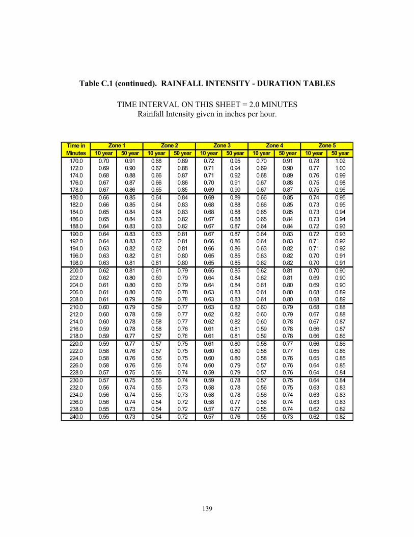
139

Table C.1 (continued). RAINFALL INTENSITY - DURATION TABLES

TIME INTERVAL ON THIS SHEET = 2.0 MINUTES Rainfall Intensity given in inches per hour.

10 year 50 year 10 year 50 year 10 year 50 year 10 year 50 year 10 year 50 year170.0 0.70 0.91 0.68 0.89 0.72 0.95 0.70 0.91 0.78 1.02172.0 0.69 0.90 0.67 0.88 0.71 0.94 0.69 0.90 0.77 1.00174.0 0.68 0.88 0.66 0.87 0.71 0.92 0.68 0.89 0.76 0.99176.0 0.67 0.87 0.66 0.86 0.70 0.91 0.67 0.88 0.75 0.98178.0 0.67 0.86 0.65 0.85 0.69 0.90 0.67 0.87 0.75 0.96180.0 0.66 0.85 0.64 0.84 0.69 0.89 0.66 0.85 0.74 0.95182.0 0.66 0.85 0.64 0.83 0.68 0.88 0.66 0.85 0.73 0.95184.0 0.65 0.84 0.64 0.83 0.68 0.88 0.65 0.85 0.73 0.94186.0 0.65 0.84 0.63 0.82 0.67 0.88 0.65 0.84 0.73 0.94188.0 0.64 0.83 0.63 0.82 0.67 0.87 0.64 0.84 0.72 0.93190.0 0.64 0.83 0.63 0.81 0.67 0.87 0.64 0.83 0.72 0.93192.0 0.64 0.83 0.62 0.81 0.66 0.86 0.64 0.83 0.71 0.92194.0 0.63 0.82 0.62 0.81 0.66 0.86 0.63 0.82 0.71 0.92196.0 0.63 0.82 0.61 0.80 0.65 0.85 0.63 0.82 0.70 0.91198.0 0.63 0.81 0.61 0.80 0.65 0.85 0.62 0.82 0.70 0.91200.0 0.62 0.81 0.61 0.79 0.65 0.85 0.62 0.81 0.70 0.90202.0 0.62 0.80 0.60 0.79 0.64 0.84 0.62 0.81 0.69 0.90204.0 0.61 0.80 0.60 0.79 0.64 0.84 0.61 0.80 0.69 0.90206.0 0.61 0.80 0.60 0.78 0.63 0.83 0.61 0.80 0.68 0.89208.0 0.61 0.79 0.59 0.78 0.63 0.83 0.61 0.80 0.68 0.89210.0 0.60 0.79 0.59 0.77 0.63 0.82 0.60 0.79 0.68 0.88212.0 0.60 0.78 0.59 0.77 0.62 0.82 0.60 0.79 0.67 0.88214.0 0.60 0.78 0.58 0.77 0.62 0.82 0.60 0.78 0.67 0.87216.0 0.59 0.78 0.58 0.76 0.61 0.81 0.59 0.78 0.66 0.87218.0 0.59 0.77 0.57 0.76 0.61 0.81 0.59 0.78 0.66 0.86220.0 0.59 0.77 0.57 0.75 0.61 0.80 0.58 0.77 0.66 0.86222.0 0.58 0.76 0.57 0.75 0.60 0.80 0.58 0.77 0.65 0.86224.0 0.58 0.76 0.56 0.75 0.60 0.80 0.58 0.76 0.65 0.85226.0 0.58 0.76 0.56 0.74 0.60 0.79 0.57 0.76 0.64 0.85228.0 0.57 0.75 0.56 0.74 0.59 0.79 0.57 0.76 0.64 0.84230.0 0.57 0.75 0.55 0.74 0.59 0.78 0.57 0.75 0.64 0.84232.0 0.56 0.74 0.55 0.73 0.58 0.78 0.56 0.75 0.63 0.83234.0 0.56 0.74 0.55 0.73 0.58 0.78 0.56 0.74 0.63 0.83236.0 0.56 0.74 0.54 0.72 0.58 0.77 0.56 0.74 0.63 0.83238.0 0.55 0.73 0.54 0.72 0.57 0.77 0.55 0.74 0.62 0.82240.0 0.55 0.73 0.54 0.72 0.57 0.76 0.55 0.73 0.62 0.82

Time in Minutes

Zone 1 Zone 2 Zone 3 Zone 4 Zone 5

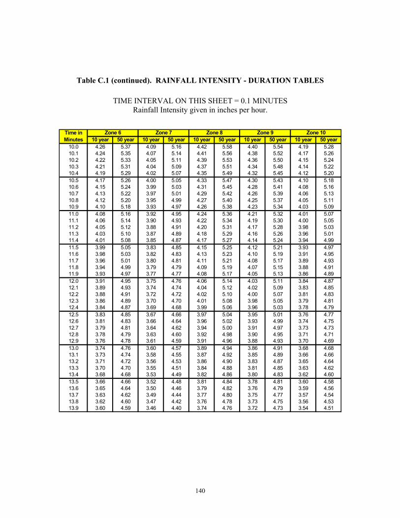
140

Table C.1 (continued). RAINFALL INTENSITY - DURATION TABLES

TIME INTERVAL ON THIS SHEET = 0.1 MINUTES Rainfall Intensity given in inches per hour.

10 year 50 year 10 year 50 year 10 year 50 year 10 year 50 year 10 year 50 year10.0 4.26 5.37 4.09 5.16 4.42 5.58 4.40 5.54 4.19 5.2810.1 4.24 5.35 4.07 5.14 4.41 5.56 4.38 5.52 4.17 5.2610.2 4.22 5.33 4.05 5.11 4.39 5.53 4.36 5.50 4.15 5.2410.3 4.21 5.31 4.04 5.09 4.37 5.51 4.34 5.48 4.14 5.2210.4 4.19 5.29 4.02 5.07 4.35 5.49 4.32 5.45 4.12 5.2010.5 4.17 5.26 4.00 5.05 4.33 5.47 4.30 5.43 4.10 5.1810.6 4.15 5.24 3.99 5.03 4.31 5.45 4.28 5.41 4.08 5.1610.7 4.13 5.22 3.97 5.01 4.29 5.42 4.26 5.39 4.06 5.1310.8 4.12 5.20 3.95 4.99 4.27 5.40 4.25 5.37 4.05 5.1110.9 4.10 5.18 3.93 4.97 4.26 5.38 4.23 5.34 4.03 5.0911.0 4.08 5.16 3.92 4.95 4.24 5.36 4.21 5.32 4.01 5.0711.1 4.06 5.14 3.90 4.93 4.22 5.34 4.19 5.30 4.00 5.0511.2 4.05 5.12 3.88 4.91 4.20 5.31 4.17 5.28 3.98 5.0311.3 4.03 5.10 3.87 4.89 4.18 5.29 4.16 5.26 3.96 5.0111.4 4.01 5.08 3.85 4.87 4.17 5.27 4.14 5.24 3.94 4.9911.5 3.99 5.05 3.83 4.85 4.15 5.25 4.12 5.21 3.93 4.9711.6 3.98 5.03 3.82 4.83 4.13 5.23 4.10 5.19 3.91 4.9511.7 3.96 5.01 3.80 4.81 4.11 5.21 4.08 5.17 3.89 4.9311.8 3.94 4.99 3.79 4.79 4.09 5.19 4.07 5.15 3.88 4.9111.9 3.93 4.97 3.77 4.77 4.08 5.17 4.05 5.13 3.86 4.8912.0 3.91 4.95 3.75 4.76 4.06 5.14 4.03 5.11 3.84 4.8712.1 3.89 4.93 3.74 4.74 4.04 5.12 4.02 5.09 3.83 4.8512.2 3.88 4.91 3.72 4.72 4.02 5.10 4.00 5.07 3.81 4.8312.3 3.86 4.89 3.70 4.70 4.01 5.08 3.98 5.05 3.79 4.8112.4 3.84 4.87 3.69 4.68 3.99 5.06 3.96 5.03 3.78 4.7912.5 3.83 4.85 3.67 4.66 3.97 5.04 3.95 5.01 3.76 4.7712.6 3.81 4.83 3.66 4.64 3.96 5.02 3.93 4.99 3.74 4.7512.7 3.79 4.81 3.64 4.62 3.94 5.00 3.91 4.97 3.73 4.7312.8 3.78 4.79 3.63 4.60 3.92 4.98 3.90 4.95 3.71 4.7112.9 3.76 4.78 3.61 4.59 3.91 4.96 3.88 4.93 3.70 4.6913.0 3.74 4.76 3.60 4.57 3.89 4.94 3.86 4.91 3.68 4.6813.1 3.73 4.74 3.58 4.55 3.87 4.92 3.85 4.89 3.66 4.6613.2 3.71 4.72 3.56 4.53 3.86 4.90 3.83 4.87 3.65 4.6413.3 3.70 4.70 3.55 4.51 3.84 4.88 3.81 4.85 3.63 4.6213.4 3.68 4.68 3.53 4.49 3.82 4.86 3.80 4.83 3.62 4.6013.5 3.66 4.66 3.52 4.48 3.81 4.84 3.78 4.81 3.60 4.5813.6 3.65 4.64 3.50 4.46 3.79 4.82 3.76 4.79 3.59 4.5613.7 3.63 4.62 3.49 4.44 3.77 4.80 3.75 4.77 3.57 4.5413.8 3.62 4.60 3.47 4.42 3.76 4.78 3.73 4.75 3.56 4.5313.9 3.60 4.59 3.46 4.40 3.74 4.76 3.72 4.73 3.54 4.51

Zone 6Time in Minutes

Zone 9 Zone 10Zone 7 Zone 8

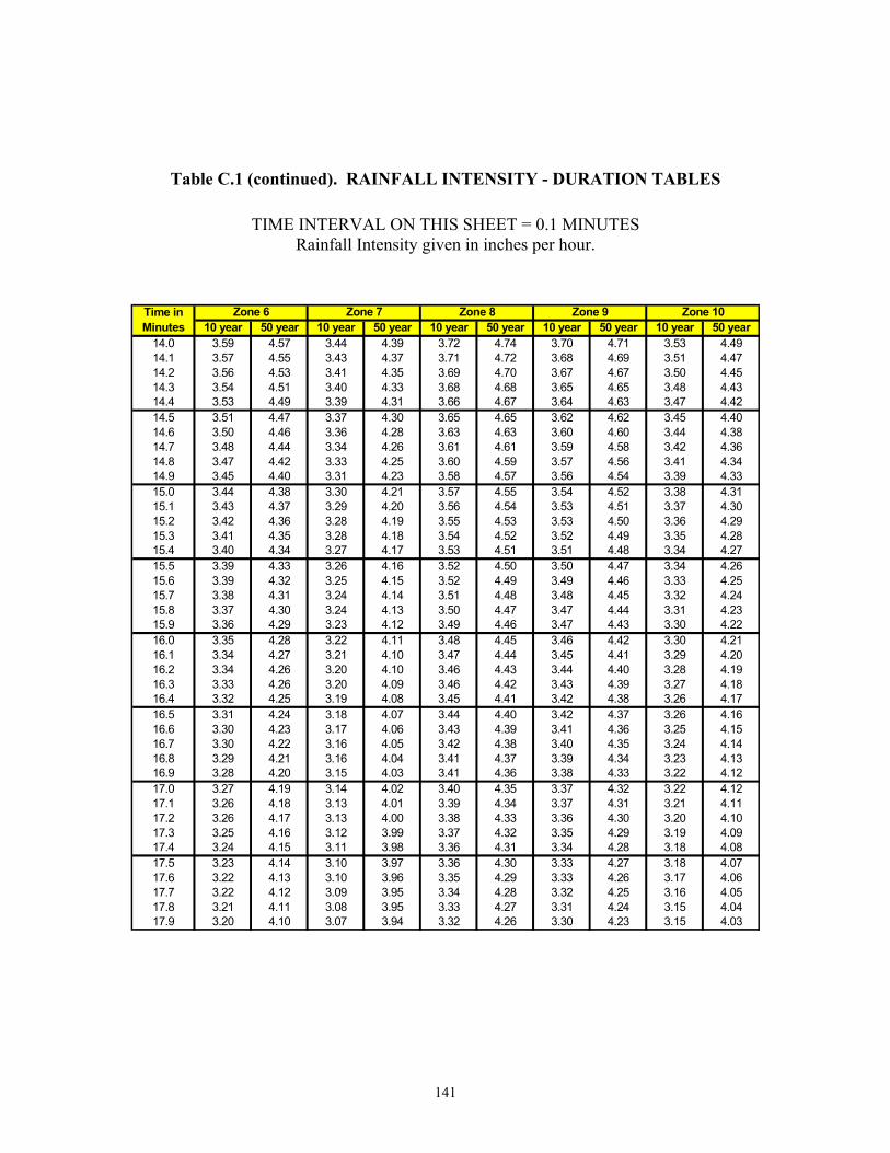
141

Table C.1 (continued). RAINFALL INTENSITY - DURATION TABLES

TIME INTERVAL ON THIS SHEET = 0.1 MINUTES Rainfall Intensity given in inches per hour.

10 year 50 year 10 year 50 year 10 year 50 year 10 year 50 year 10 year 50 year14.0 3.59 4.57 3.44 4.39 3.72 4.74 3.70 4.71 3.53 4.4914.1 3.57 4.55 3.43 4.37 3.71 4.72 3.68 4.69 3.51 4.4714.2 3.56 4.53 3.41 4.35 3.69 4.70 3.67 4.67 3.50 4.4514.3 3.54 4.51 3.40 4.33 3.68 4.68 3.65 4.65 3.48 4.4314.4 3.53 4.49 3.39 4.31 3.66 4.67 3.64 4.63 3.47 4.4214.5 3.51 4.47 3.37 4.30 3.65 4.65 3.62 4.62 3.45 4.4014.6 3.50 4.46 3.36 4.28 3.63 4.63 3.60 4.60 3.44 4.3814.7 3.48 4.44 3.34 4.26 3.61 4.61 3.59 4.58 3.42 4.3614.8 3.47 4.42 3.33 4.25 3.60 4.59 3.57 4.56 3.41 4.3414.9 3.45 4.40 3.31 4.23 3.58 4.57 3.56 4.54 3.39 4.3315.0 3.44 4.38 3.30 4.21 3.57 4.55 3.54 4.52 3.38 4.3115.1 3.43 4.37 3.29 4.20 3.56 4.54 3.53 4.51 3.37 4.3015.2 3.42 4.36 3.28 4.19 3.55 4.53 3.53 4.50 3.36 4.2915.3 3.41 4.35 3.28 4.18 3.54 4.52 3.52 4.49 3.35 4.2815.4 3.40 4.34 3.27 4.17 3.53 4.51 3.51 4.48 3.34 4.2715.5 3.39 4.33 3.26 4.16 3.52 4.50 3.50 4.47 3.34 4.2615.6 3.39 4.32 3.25 4.15 3.52 4.49 3.49 4.46 3.33 4.2515.7 3.38 4.31 3.24 4.14 3.51 4.48 3.48 4.45 3.32 4.2415.8 3.37 4.30 3.24 4.13 3.50 4.47 3.47 4.44 3.31 4.2315.9 3.36 4.29 3.23 4.12 3.49 4.46 3.47 4.43 3.30 4.2216.0 3.35 4.28 3.22 4.11 3.48 4.45 3.46 4.42 3.30 4.2116.1 3.34 4.27 3.21 4.10 3.47 4.44 3.45 4.41 3.29 4.2016.2 3.34 4.26 3.20 4.10 3.46 4.43 3.44 4.40 3.28 4.1916.3 3.33 4.26 3.20 4.09 3.46 4.42 3.43 4.39 3.27 4.1816.4 3.32 4.25 3.19 4.08 3.45 4.41 3.42 4.38 3.26 4.1716.5 3.31 4.24 3.18 4.07 3.44 4.40 3.42 4.37 3.26 4.1616.6 3.30 4.23 3.17 4.06 3.43 4.39 3.41 4.36 3.25 4.1516.7 3.30 4.22 3.16 4.05 3.42 4.38 3.40 4.35 3.24 4.1416.8 3.29 4.21 3.16 4.04 3.41 4.37 3.39 4.34 3.23 4.1316.9 3.28 4.20 3.15 4.03 3.41 4.36 3.38 4.33 3.22 4.1217.0 3.27 4.19 3.14 4.02 3.40 4.35 3.37 4.32 3.22 4.1217.1 3.26 4.18 3.13 4.01 3.39 4.34 3.37 4.31 3.21 4.1117.2 3.26 4.17 3.13 4.00 3.38 4.33 3.36 4.30 3.20 4.1017.3 3.25 4.16 3.12 3.99 3.37 4.32 3.35 4.29 3.19 4.0917.4 3.24 4.15 3.11 3.98 3.36 4.31 3.34 4.28 3.18 4.0817.5 3.23 4.14 3.10 3.97 3.36 4.30 3.33 4.27 3.18 4.0717.6 3.22 4.13 3.10 3.96 3.35 4.29 3.33 4.26 3.17 4.0617.7 3.22 4.12 3.09 3.95 3.34 4.28 3.32 4.25 3.16 4.0517.8 3.21 4.11 3.08 3.95 3.33 4.27 3.31 4.24 3.15 4.0417.9 3.20 4.10 3.07 3.94 3.32 4.26 3.30 4.23 3.15 4.03

Zone 6 Zone 7 Zone 8Time in Minutes

Zone 9 Zone 10

142

Table C.1 (continued). RAINFALL INTENSITY - DURATION TABLES

TIME INTERVAL ON THIS SHEET = 0.1 MINUTES Rainfall Intensity given in inches per hour.

10 year 50 year 10 year 50 year 10 year 50 year 10 year 50 year 10 year 50 year18.0 3.19 4.09 3.07 3.93 3.32 4.25 3.29 4.22 3.14 4.0218.1 3.19 4.08 3.06 3.92 3.31 4.24 3.29 4.21 3.13 4.0118.2 3.18 4.07 3.05 3.91 3.30 4.23 3.28 4.20 3.12 4.0018.3 3.17 4.06 3.04 3.90 3.29 4.22 3.27 4.19 3.12 3.9918.4 3.16 4.05 3.04 3.89 3.28 4.21 3.26 4.18 3.11 3.9818.5 3.15 4.04 3.03 3.88 3.28 4.20 3.25 4.17 3.10 3.9718.6 3.15 4.03 3.02 3.87 3.27 4.19 3.25 4.16 3.09 3.9718.7 3.14 4.03 3.01 3.86 3.26 4.18 3.24 4.15 3.09 3.9618.8 3.13 4.02 3.01 3.86 3.25 4.17 3.23 4.14 3.08 3.9518.9 3.12 4.01 3.00 3.85 3.24 4.16 3.22 4.13 3.07 3.9419.0 3.12 4.00 2.99 3.84 3.24 4.15 3.21 4.12 3.06 3.9319.1 3.11 3.99 2.98 3.83 3.23 4.14 3.21 4.11 3.06 3.9219.2 3.10 3.98 2.98 3.82 3.22 4.13 3.20 4.10 3.05 3.9119.3 3.09 3.97 2.97 3.81 3.21 4.12 3.19 4.09 3.04 3.9019.4 3.09 3.96 2.96 3.80 3.20 4.11 3.18 4.08 3.03 3.8919.5 3.08 3.95 2.95 3.79 3.20 4.10 3.17 4.08 3.03 3.8819.6 3.07 3.94 2.95 3.78 3.19 4.09 3.17 4.07 3.02 3.8819.7 3.06 3.93 2.94 3.78 3.18 4.08 3.16 4.06 3.01 3.8719.8 3.06 3.92 2.93 3.77 3.17 4.08 3.15 4.05 3.00 3.8619.9 3.05 3.91 2.93 3.76 3.17 4.07 3.14 4.04 3.00 3.8520.0 3.04 3.91 2.92 3.75 3.16 4.06 3.14 4.03 2.99 3.8420.1 3.03 3.90 2.91 3.74 3.15 4.05 3.13 4.02 2.98 3.8320.2 3.03 3.89 2.90 3.73 3.14 4.04 3.12 4.01 2.97 3.8220.3 3.02 3.88 2.90 3.72 3.13 4.03 3.11 4.00 2.97 3.8120.4 3.01 3.87 2.89 3.71 3.13 4.02 3.11 3.99 2.96 3.8020.5 3.00 3.86 2.88 3.71 3.12 4.01 3.10 3.98 2.95 3.8020.6 3.00 3.85 2.88 3.70 3.11 4.00 3.09 3.97 2.95 3.7920.7 2.99 3.84 2.87 3.69 3.10 3.99 3.08 3.96 2.94 3.7820.8 2.98 3.83 2.86 3.68 3.10 3.98 3.08 3.95 2.93 3.7720.9 2.97 3.83 2.85 3.67 3.09 3.97 3.07 3.95 2.92 3.7621.0 2.97 3.82 2.85 3.66 3.08 3.96 3.06 3.94 2.92 3.7521.1 2.96 3.81 2.84 3.65 3.07 3.95 3.05 3.93 2.91 3.7421.2 2.95 3.80 2.83 3.65 3.07 3.95 3.05 3.92 2.90 3.7321.3 2.95 3.79 2.83 3.64 3.06 3.94 3.04 3.91 2.90 3.7321.4 2.94 3.78 2.82 3.63 3.05 3.93 3.03 3.90 2.89 3.7221.5 2.93 3.77 2.81 3.62 3.04 3.92 3.02 3.89 2.88 3.7121.6 2.92 3.76 2.81 3.61 3.04 3.91 3.02 3.88 2.87 3.7021.7 2.92 3.76 2.80 3.60 3.03 3.90 3.01 3.87 2.87 3.6921.8 2.91 3.75 2.79 3.60 3.02 3.89 3.00 3.86 2.86 3.6821.9 2.90 3.74 2.79 3.59 3.01 3.88 2.99 3.86 2.85 3.67

Zone 6Time in Minutes

Zone 9 Zone 10Zone 7 Zone 8

143

Table C.1 (continued). RAINFALL INTENSITY - DURATION TABLES

TIME INTERVAL ON THIS SHEET = 0.1 MINUTES Rainfall Intensity given in inches per hour.

10 year 50 year 10 year 50 year 10 year 50 year 10 year 50 year 10 year 50 year22.0 2.90 3.73 2.78 3.58 3.01 3.87 2.99 3.85 2.85 3.6722.1 2.89 3.72 2.77 3.57 3.00 3.86 2.98 3.84 2.84 3.6622.2 2.88 3.71 2.76 3.56 2.99 3.86 2.97 3.83 2.83 3.6522.3 2.87 3.70 2.76 3.55 2.99 3.85 2.96 3.82 2.83 3.6422.4 2.87 3.69 2.75 3.55 2.98 3.84 2.96 3.81 2.82 3.6322.5 2.86 3.69 2.74 3.54 2.97 3.83 2.95 3.80 2.81 3.6222.6 2.85 3.68 2.74 3.53 2.96 3.82 2.94 3.79 2.81 3.6222.7 2.85 3.67 2.73 3.52 2.96 3.81 2.94 3.79 2.80 3.6122.8 2.84 3.66 2.72 3.51 2.95 3.80 2.93 3.78 2.79 3.6022.9 2.83 3.65 2.72 3.50 2.94 3.79 2.92 3.77 2.78 3.5923.0 2.83 3.64 2.71 3.50 2.93 3.78 2.91 3.76 2.78 3.5823.1 2.82 3.64 2.70 3.49 2.93 3.78 2.91 3.75 2.77 3.5723.2 2.81 3.63 2.70 3.48 2.92 3.77 2.90 3.74 2.76 3.5723.3 2.81 3.62 2.69 3.47 2.91 3.76 2.89 3.73 2.76 3.5623.4 2.80 3.61 2.68 3.46 2.91 3.75 2.89 3.72 2.75 3.5523.5 2.79 3.60 2.68 3.46 2.90 3.74 2.88 3.72 2.74 3.5423.6 2.78 3.59 2.67 3.45 2.89 3.73 2.87 3.71 2.74 3.5323.7 2.78 3.59 2.66 3.44 2.88 3.72 2.87 3.70 2.73 3.5323.8 2.77 3.58 2.66 3.43 2.88 3.72 2.86 3.69 2.72 3.5223.9 2.76 3.57 2.65 3.42 2.87 3.71 2.85 3.68 2.72 3.5124.0 2.76 3.56 2.65 3.42 2.86 3.70 2.84 3.67 2.71 3.5024.1 2.75 3.55 2.64 3.41 2.86 3.69 2.84 3.66 2.70 3.4924.2 2.74 3.54 2.63 3.40 2.85 3.68 2.83 3.66 2.70 3.4824.3 2.74 3.54 2.63 3.39 2.84 3.67 2.82 3.65 2.69 3.4824.4 2.73 3.53 2.62 3.38 2.84 3.66 2.82 3.64 2.68 3.4724.5 2.72 3.52 2.61 3.38 2.83 3.66 2.81 3.63 2.68 3.4624.6 2.72 3.51 2.61 3.37 2.82 3.65 2.80 3.62 2.67 3.4524.7 2.71 3.50 2.60 3.36 2.82 3.64 2.80 3.61 2.67 3.4424.8 2.70 3.50 2.59 3.35 2.81 3.63 2.79 3.61 2.66 3.4424.9 2.70 3.49 2.59 3.34 2.80 3.62 2.78 3.60 2.65 3.4325.0 2.69 3.48 2.58 3.34 2.79 3.61 2.78 3.59 2.65 3.4225.1 2.68 3.47 2.57 3.33 2.79 3.61 2.77 3.58 2.64 3.4125.2 2.68 3.46 2.57 3.32 2.78 3.60 2.76 3.57 2.63 3.4125.3 2.67 3.46 2.56 3.31 2.77 3.59 2.76 3.56 2.63 3.4025.4 2.66 3.45 2.56 3.31 2.77 3.58 2.75 3.56 2.62 3.3925.5 2.66 3.44 2.55 3.30 2.76 3.57 2.74 3.55 2.61 3.3825.6 2.65 3.43 2.54 3.29 2.75 3.56 2.74 3.54 2.61 3.3725.7 2.65 3.42 2.54 3.28 2.75 3.56 2.73 3.53 2.60 3.3725.8 2.64 3.42 2.53 3.28 2.74 3.55 2.72 3.52 2.59 3.3625.9 2.63 3.41 2.52 3.27 2.73 3.54 2.72 3.52 2.59 3.35

Zone 6 Zone 7 Zone 8Time in Minutes

Zone 9 Zone 10

144

Table C.1 (continued). RAINFALL INTENSITY - DURATION TABLES

TIME INTERVAL ON THIS SHEET = 0.1 MINUTES Rainfall Intensity given in inches per hour.

10 year 50 year 10 year 50 year 10 year 50 year 10 year 50 year 10 year 50 year26.0 2.63 3.40 2.52 3.26 2.73 3.53 2.71 3.51 2.58 3.3426.1 2.62 3.39 2.51 3.25 2.72 3.52 2.70 3.50 2.58 3.3426.2 2.61 3.38 2.51 3.25 2.71 3.51 2.70 3.49 2.57 3.3326.3 2.61 3.38 2.50 3.24 2.71 3.51 2.69 3.48 2.56 3.3226.4 2.60 3.37 2.49 3.23 2.70 3.50 2.68 3.47 2.56 3.3126.5 2.59 3.36 2.49 3.22 2.69 3.49 2.68 3.47 2.55 3.3026.6 2.59 3.35 2.48 3.22 2.69 3.48 2.67 3.46 2.54 3.3026.7 2.58 3.35 2.48 3.21 2.68 3.47 2.66 3.45 2.54 3.2926.8 2.58 3.34 2.47 3.20 2.67 3.47 2.66 3.44 2.53 3.2826.9 2.57 3.33 2.46 3.19 2.67 3.46 2.65 3.43 2.53 3.2727.0 2.56 3.32 2.46 3.19 2.66 3.45 2.64 3.43 2.52 3.2727.1 2.56 3.31 2.45 3.18 2.65 3.44 2.64 3.42 2.51 3.2627.2 2.55 3.31 2.45 3.17 2.65 3.43 2.63 3.41 2.51 3.2527.3 2.54 3.30 2.44 3.16 2.64 3.43 2.62 3.40 2.50 3.2427.4 2.54 3.29 2.43 3.16 2.64 3.42 2.62 3.40 2.50 3.2427.5 2.53 3.28 2.43 3.15 2.63 3.41 2.61 3.39 2.49 3.2327.6 2.53 3.28 2.42 3.14 2.62 3.40 2.61 3.38 2.48 3.2227.7 2.52 3.27 2.42 3.13 2.62 3.39 2.60 3.37 2.48 3.2127.8 2.51 3.26 2.41 3.13 2.61 3.39 2.59 3.36 2.47 3.2127.9 2.51 3.25 2.40 3.12 2.60 3.38 2.59 3.36 2.47 3.2028.0 2.50 3.25 2.40 3.11 2.60 3.37 2.58 3.35 2.46 3.1928.1 2.49 3.24 2.39 3.10 2.59 3.36 2.57 3.34 2.45 3.1828.2 2.49 3.23 2.39 3.10 2.58 3.36 2.57 3.33 2.45 3.1828.3 2.48 3.22 2.38 3.09 2.58 3.35 2.56 3.33 2.44 3.1728.4 2.48 3.22 2.37 3.08 2.57 3.34 2.55 3.32 2.44 3.1628.5 2.47 3.21 2.37 3.08 2.57 3.33 2.55 3.31 2.43 3.1628.6 2.46 3.20 2.36 3.07 2.56 3.32 2.54 3.30 2.42 3.1528.7 2.46 3.19 2.36 3.06 2.55 3.32 2.54 3.29 2.42 3.1428.8 2.45 3.19 2.35 3.05 2.55 3.31 2.53 3.29 2.41 3.1328.9 2.45 3.18 2.35 3.05 2.54 3.30 2.52 3.28 2.41 3.1329.0 2.44 3.17 2.34 3.04 2.53 3.29 2.52 3.27 2.40 3.1229.1 2.43 3.16 2.33 3.03 2.53 3.29 2.51 3.26 2.39 3.1129.2 2.43 3.16 2.33 3.03 2.52 3.28 2.51 3.26 2.39 3.1029.3 2.42 3.15 2.32 3.02 2.52 3.27 2.50 3.25 2.38 3.1029.4 2.42 3.14 2.32 3.01 2.51 3.26 2.49 3.24 2.38 3.0929.5 2.41 3.14 2.31 3.01 2.50 3.26 2.49 3.23 2.37 3.0829.6 2.40 3.13 2.31 3.00 2.50 3.25 2.48 3.23 2.37 3.0829.7 2.40 3.12 2.30 2.99 2.49 3.24 2.47 3.22 2.36 3.0729.8 2.39 3.11 2.29 2.98 2.49 3.23 2.47 3.21 2.35 3.0629.9 2.39 3.11 2.29 2.98 2.48 3.23 2.46 3.20 2.35 3.06

Zone 6Time in Minutes

Zone 9 Zone 10Zone 7 Zone 8

145

Table C.1 (continued). RAINFALL INTENSITY - DURATION TABLES

TIME INTERVAL ON THIS SHEET = 0.2 MINUTES Rainfall Intensity given in inches per hour.

10 year 50 year 10 year 50 year 10 year 50 year 10 year 50 year 10 year 50 year30.0 2.38 3.10 2.28 2.97 2.47 3.22 2.46 3.20 2.34 3.0530.2 2.38 3.09 2.28 2.96 2.47 3.21 2.45 3.19 2.34 3.0430.4 2.37 3.09 2.27 2.96 2.46 3.21 2.45 3.18 2.33 3.0430.6 2.36 3.08 2.27 2.95 2.46 3.20 2.44 3.18 2.33 3.0330.8 2.36 3.08 2.26 2.95 2.45 3.19 2.43 3.17 2.32 3.0231.0 2.35 3.07 2.25 2.94 2.44 3.19 2.43 3.16 2.32 3.0231.2 2.35 3.07 2.25 2.94 2.44 3.18 2.42 3.16 2.31 3.0131.4 2.34 3.06 2.24 2.93 2.43 3.17 2.42 3.15 2.30 3.0031.6 2.34 3.05 2.24 2.92 2.43 3.17 2.41 3.15 2.30 3.0031.8 2.33 3.05 2.23 2.92 2.42 3.16 2.41 3.14 2.29 2.9932.0 2.33 3.04 2.23 2.91 2.42 3.15 2.40 3.13 2.29 2.9832.2 2.32 3.04 2.22 2.91 2.41 3.15 2.40 3.13 2.28 2.9832.4 2.31 3.03 2.22 2.90 2.40 3.14 2.39 3.12 2.28 2.9732.6 2.31 3.03 2.21 2.90 2.40 3.13 2.38 3.11 2.27 2.9732.8 2.30 3.02 2.20 2.89 2.39 3.13 2.38 3.11 2.27 2.9633.0 2.30 3.02 2.20 2.88 2.39 3.12 2.37 3.10 2.26 2.9533.2 2.29 3.01 2.19 2.88 2.38 3.12 2.37 3.09 2.26 2.9533.4 2.29 3.00 2.19 2.87 2.38 3.11 2.36 3.09 2.25 2.9433.6 2.28 3.00 2.18 2.87 2.37 3.10 2.36 3.08 2.25 2.9433.8 2.28 2.99 2.18 2.86 2.37 3.10 2.35 3.08 2.24 2.9334.0 2.27 2.99 2.17 2.86 2.36 3.09 2.35 3.07 2.24 2.9234.2 2.26 2.98 2.17 2.85 2.35 3.08 2.34 3.06 2.23 2.9234.4 2.26 2.98 2.16 2.85 2.35 3.08 2.33 3.06 2.23 2.9134.6 2.25 2.97 2.16 2.84 2.34 3.07 2.33 3.05 2.22 2.9034.8 2.25 2.97 2.15 2.83 2.34 3.07 2.32 3.04 2.22 2.9035.0 2.24 2.96 2.15 2.83 2.33 3.06 2.32 3.04 2.21 2.8935.2 2.24 2.96 2.14 2.82 2.33 3.05 2.31 3.03 2.21 2.8935.4 2.23 2.95 2.13 2.82 2.32 3.05 2.31 3.03 2.20 2.8835.6 2.23 2.94 2.13 2.81 2.32 3.04 2.30 3.02 2.20 2.8735.8 2.22 2.94 2.12 2.81 2.31 3.03 2.30 3.01 2.19 2.8736.0 2.22 2.93 2.12 2.80 2.31 3.03 2.29 3.01 2.19 2.8636.2 2.21 2.93 2.11 2.80 2.30 3.02 2.29 3.00 2.18 2.8636.4 2.21 2.92 2.11 2.79 2.29 3.02 2.28 3.00 2.18 2.8536.6 2.20 2.92 2.10 2.79 2.29 3.01 2.28 2.99 2.17 2.8436.8 2.20 2.91 2.10 2.78 2.28 3.00 2.27 2.98 2.17 2.8437.0 2.19 2.91 2.09 2.77 2.28 3.00 2.27 2.98 2.16 2.8337.2 2.19 2.90 2.09 2.77 2.27 2.99 2.26 2.97 2.16 2.8337.4 2.18 2.90 2.08 2.76 2.27 2.98 2.25 2.96 2.15 2.8237.6 2.17 2.89 2.08 2.76 2.26 2.98 2.25 2.96 2.15 2.8137.8 2.17 2.89 2.07 2.75 2.26 2.97 2.24 2.95 2.14 2.81

Zone 6 Zone 7 Zone 8Time in Minutes

Zone 9 Zone 10

146

Table C.1 (continued). RAINFALL INTENSITY - DURATION TABLES

TIME INTERVAL ON THIS SHEET = 0.5 MINUTES Rainfall Intensity given in inches per hour.

10 year 50 year 10 year 50 year 10 year 50 year 10 year 50 year 10 year 50 year38.0 2.16 2.88 2.07 2.75 2.25 2.97 2.24 2.95 2.14 2.8038.5 2.15 2.87 2.05 2.73 2.24 2.95 2.23 2.93 2.12 2.7939.0 2.14 2.85 2.04 2.72 2.23 2.94 2.21 2.92 2.11 2.7739.5 2.13 2.84 2.03 2.71 2.21 2.92 2.20 2.90 2.10 2.7640.0 2.11 2.83 2.02 2.69 2.20 2.91 2.19 2.89 2.09 2.7440.5 2.10 2.82 2.00 2.68 2.19 2.89 2.18 2.87 2.08 2.7341.0 2.09 2.80 1.99 2.67 2.17 2.88 2.16 2.86 2.06 2.7241.5 2.08 2.79 1.98 2.66 2.16 2.86 2.15 2.84 2.05 2.7042.0 2.06 2.78 1.97 2.64 2.15 2.85 2.14 2.83 2.04 2.6942.5 2.05 2.76 1.95 2.63 2.14 2.83 2.13 2.81 2.03 2.6743.0 2.04 2.75 1.94 2.62 2.12 2.82 2.11 2.80 2.02 2.6643.5 2.03 2.74 1.93 2.60 2.11 2.80 2.10 2.79 2.01 2.6544.0 2.02 2.73 1.92 2.59 2.10 2.79 2.09 2.77 1.99 2.6344.5 2.00 2.71 1.91 2.58 2.09 2.78 2.08 2.76 1.98 2.6245.0 1.99 2.70 1.90 2.57 2.07 2.76 2.06 2.74 1.97 2.6045.5 1.98 2.69 1.88 2.55 2.06 2.75 2.05 2.73 1.96 2.5946.0 1.97 2.68 1.87 2.54 2.05 2.73 2.04 2.72 1.95 2.5846.5 1.96 2.66 1.86 2.53 2.04 2.72 2.03 2.70 1.94 2.5647.0 1.94 2.65 1.85 2.52 2.03 2.71 2.02 2.69 1.93 2.5547.5 1.93 2.64 1.84 2.50 2.01 2.69 2.01 2.67 1.92 2.5448.0 1.92 2.63 1.83 2.49 2.00 2.68 1.99 2.66 1.91 2.5248.5 1.91 2.62 1.81 2.48 1.99 2.67 1.98 2.65 1.89 2.5149.0 1.90 2.60 1.80 2.47 1.98 2.65 1.97 2.63 1.88 2.5049.5 1.89 2.59 1.79 2.46 1.97 2.64 1.96 2.62 1.87 2.4850.0 1.88 2.58 1.78 2.44 1.96 2.62 1.95 2.61 1.86 2.4750.5 1.86 2.57 1.77 2.43 1.94 2.61 1.94 2.59 1.85 2.4651.0 1.85 2.56 1.76 2.42 1.93 2.60 1.93 2.58 1.84 2.4551.5 1.84 2.55 1.75 2.41 1.92 2.59 1.92 2.57 1.83 2.4352.0 1.83 2.53 1.74 2.40 1.91 2.57 1.90 2.55 1.82 2.4252.5 1.82 2.52 1.73 2.38 1.90 2.56 1.89 2.54 1.81 2.4153.0 1.81 2.51 1.72 2.37 1.89 2.55 1.88 2.53 1.80 2.3953.5 1.80 2.50 1.71 2.36 1.88 2.53 1.87 2.51 1.79 2.3854.0 1.79 2.49 1.70 2.35 1.87 2.52 1.86 2.50 1.78 2.3754.5 1.78 2.48 1.68 2.34 1.85 2.51 1.85 2.49 1.77 2.3655.0 1.77 2.47 1.67 2.33 1.84 2.49 1.84 2.48 1.76 2.3455.5 1.76 2.45 1.66 2.32 1.83 2.48 1.83 2.46 1.75 2.3356.0 1.75 2.44 1.65 2.30 1.82 2.47 1.82 2.45 1.74 2.3256.5 1.74 2.43 1.64 2.29 1.81 2.46 1.81 2.44 1.73 2.3157.0 1.73 2.42 1.63 2.28 1.80 2.44 1.80 2.43 1.72 2.3057.5 1.72 2.41 1.62 2.27 1.79 2.43 1.79 2.41 1.71 2.28

Zone 8Zone 6Time in Minutes

Zone 9 Zone 10Zone 7

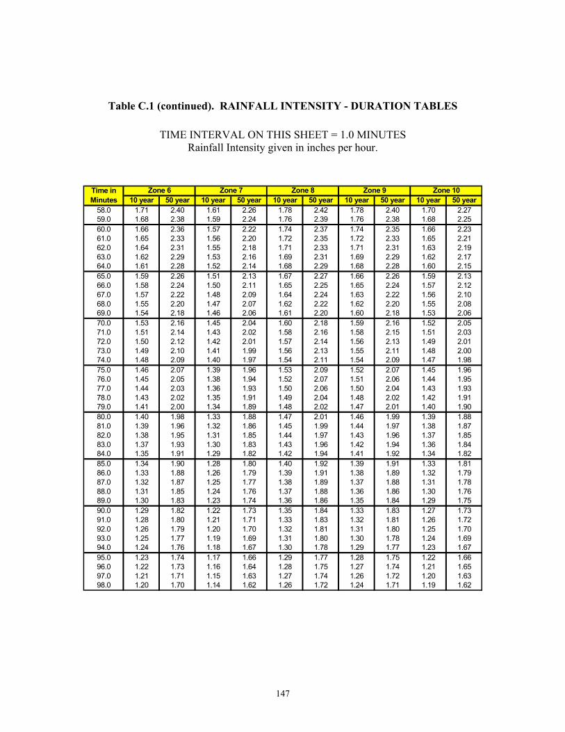
147

Table C.1 (continued). RAINFALL INTENSITY - DURATION TABLES

TIME INTERVAL ON THIS SHEET = 1.0 MINUTES Rainfall Intensity given in inches per hour.

10 year 50 year 10 year 50 year 10 year 50 year 10 year 50 year 10 year 50 year58.0 1.71 2.40 1.61 2.26 1.78 2.42 1.78 2.40 1.70 2.2759.0 1.68 2.38 1.59 2.24 1.76 2.39 1.76 2.38 1.68 2.2560.0 1.66 2.36 1.57 2.22 1.74 2.37 1.74 2.35 1.66 2.2361.0 1.65 2.33 1.56 2.20 1.72 2.35 1.72 2.33 1.65 2.2162.0 1.64 2.31 1.55 2.18 1.71 2.33 1.71 2.31 1.63 2.1963.0 1.62 2.29 1.53 2.16 1.69 2.31 1.69 2.29 1.62 2.1764.0 1.61 2.28 1.52 2.14 1.68 2.29 1.68 2.28 1.60 2.1565.0 1.59 2.26 1.51 2.13 1.67 2.27 1.66 2.26 1.59 2.1366.0 1.58 2.24 1.50 2.11 1.65 2.25 1.65 2.24 1.57 2.1267.0 1.57 2.22 1.48 2.09 1.64 2.24 1.63 2.22 1.56 2.1068.0 1.55 2.20 1.47 2.07 1.62 2.22 1.62 2.20 1.55 2.0869.0 1.54 2.18 1.46 2.06 1.61 2.20 1.60 2.18 1.53 2.0670.0 1.53 2.16 1.45 2.04 1.60 2.18 1.59 2.16 1.52 2.0571.0 1.51 2.14 1.43 2.02 1.58 2.16 1.58 2.15 1.51 2.0372.0 1.50 2.12 1.42 2.01 1.57 2.14 1.56 2.13 1.49 2.0173.0 1.49 2.10 1.41 1.99 1.56 2.13 1.55 2.11 1.48 2.0074.0 1.48 2.09 1.40 1.97 1.54 2.11 1.54 2.09 1.47 1.9875.0 1.46 2.07 1.39 1.96 1.53 2.09 1.52 2.07 1.45 1.9676.0 1.45 2.05 1.38 1.94 1.52 2.07 1.51 2.06 1.44 1.9577.0 1.44 2.03 1.36 1.93 1.50 2.06 1.50 2.04 1.43 1.9378.0 1.43 2.02 1.35 1.91 1.49 2.04 1.48 2.02 1.42 1.9179.0 1.41 2.00 1.34 1.89 1.48 2.02 1.47 2.01 1.40 1.9080.0 1.40 1.98 1.33 1.88 1.47 2.01 1.46 1.99 1.39 1.8881.0 1.39 1.96 1.32 1.86 1.45 1.99 1.44 1.97 1.38 1.8782.0 1.38 1.95 1.31 1.85 1.44 1.97 1.43 1.96 1.37 1.8583.0 1.37 1.93 1.30 1.83 1.43 1.96 1.42 1.94 1.36 1.8484.0 1.35 1.91 1.29 1.82 1.42 1.94 1.41 1.92 1.34 1.8285.0 1.34 1.90 1.28 1.80 1.40 1.92 1.39 1.91 1.33 1.8186.0 1.33 1.88 1.26 1.79 1.39 1.91 1.38 1.89 1.32 1.7987.0 1.32 1.87 1.25 1.77 1.38 1.89 1.37 1.88 1.31 1.7888.0 1.31 1.85 1.24 1.76 1.37 1.88 1.36 1.86 1.30 1.7689.0 1.30 1.83 1.23 1.74 1.36 1.86 1.35 1.84 1.29 1.7590.0 1.29 1.82 1.22 1.73 1.35 1.84 1.33 1.83 1.27 1.7391.0 1.28 1.80 1.21 1.71 1.33 1.83 1.32 1.81 1.26 1.7292.0 1.26 1.79 1.20 1.70 1.32 1.81 1.31 1.80 1.25 1.7093.0 1.25 1.77 1.19 1.69 1.31 1.80 1.30 1.78 1.24 1.6994.0 1.24 1.76 1.18 1.67 1.30 1.78 1.29 1.77 1.23 1.6795.0 1.23 1.74 1.17 1.66 1.29 1.77 1.28 1.75 1.22 1.6696.0 1.22 1.73 1.16 1.64 1.28 1.75 1.27 1.74 1.21 1.6597.0 1.21 1.71 1.15 1.63 1.27 1.74 1.26 1.72 1.20 1.6398.0 1.20 1.70 1.14 1.62 1.26 1.72 1.24 1.71 1.19 1.62

Zone 6 Zone 7 Zone 8Time in Minutes

Zone 9 Zone 10

148

Table C.1 (continued). RAINFALL INTENSITY - DURATION TABLES

TIME INTERVAL ON THIS SHEET = 2.0 MINUTES Rainfall Intensity given in inches per hour.

10 year 50 year 10 year 50 year 10 year 50 year 10 year 50 year 10 year 50 year100.0 1.18 1.67 1.12 1.59 1.24 1.70 1.22 1.68 1.17 1.59102.0 1.16 1.64 1.11 1.56 1.21 1.67 1.20 1.65 1.15 1.57104.0 1.14 1.61 1.09 1.54 1.19 1.64 1.18 1.63 1.13 1.54106.0 1.12 1.58 1.07 1.51 1.17 1.61 1.16 1.60 1.11 1.51108.0 1.10 1.56 1.05 1.49 1.15 1.59 1.14 1.57 1.09 1.49110.0 1.08 1.53 1.03 1.46 1.13 1.56 1.12 1.55 1.07 1.46112.0 1.06 1.50 1.02 1.44 1.11 1.53 1.10 1.52 1.05 1.44114.0 1.05 1.48 1.00 1.42 1.10 1.51 1.08 1.49 1.03 1.42116.0 1.03 1.45 0.98 1.39 1.08 1.48 1.06 1.47 1.01 1.39118.0 1.01 1.43 0.97 1.37 1.06 1.46 1.04 1.44 1.00 1.37120.0 0.99 1.40 0.95 1.35 1.04 1.44 1.03 1.42 0.98 1.35122.0 0.98 1.38 0.94 1.33 1.03 1.42 1.02 1.40 0.97 1.33124.0 0.97 1.37 0.93 1.31 1.02 1.40 1.01 1.39 0.96 1.31126.0 0.96 1.35 0.92 1.30 1.01 1.38 1.00 1.37 0.95 1.30128.0 0.95 1.33 0.91 1.28 1.00 1.37 0.98 1.35 0.94 1.28130.0 0.94 1.31 0.90 1.26 0.99 1.35 0.97 1.33 0.93 1.27132.0 0.93 1.30 0.89 1.24 0.98 1.33 0.96 1.32 0.92 1.25134.0 0.92 1.28 0.88 1.23 0.97 1.32 0.95 1.30 0.91 1.23136.0 0.92 1.26 0.87 1.21 0.96 1.30 0.94 1.28 0.90 1.22138.0 0.91 1.25 0.86 1.20 0.95 1.28 0.94 1.27 0.89 1.20140.0 0.90 1.23 0.86 1.18 0.94 1.27 0.93 1.25 0.88 1.19142.0 0.89 1.21 0.85 1.16 0.93 1.25 0.92 1.24 0.87 1.17144.0 0.88 1.20 0.84 1.15 0.92 1.24 0.91 1.22 0.86 1.16146.0 0.87 1.18 0.83 1.13 0.91 1.22 0.90 1.21 0.85 1.15148.0 0.86 1.17 0.82 1.12 0.90 1.21 0.89 1.19 0.85 1.13150.0 0.85 1.15 0.81 1.10 0.89 1.19 0.88 1.18 0.84 1.12152.0 0.84 1.13 0.80 1.09 0.88 1.18 0.87 1.16 0.83 1.10154.0 0.83 1.12 0.79 1.07 0.87 1.16 0.86 1.15 0.82 1.09156.0 0.83 1.11 0.79 1.06 0.86 1.15 0.85 1.13 0.81 1.08158.0 0.82 1.09 0.78 1.05 0.86 1.13 0.84 1.12 0.80 1.06160.0 0.81 1.08 0.77 1.03 0.85 1.12 0.83 1.10 0.80 1.05162.0 0.80 1.06 0.76 1.02 0.84 1.10 0.83 1.09 0.79 1.04164.0 0.79 1.05 0.75 1.01 0.83 1.09 0.82 1.08 0.78 1.02166.0 0.78 1.03 0.75 0.99 0.82 1.08 0.81 1.06 0.77 1.01168.0 0.78 1.02 0.74 0.98 0.81 1.06 0.80 1.05 0.76 1.00

Zone 6 Zone 7Time in Minutes

Zone 9 Zone 10Zone 8

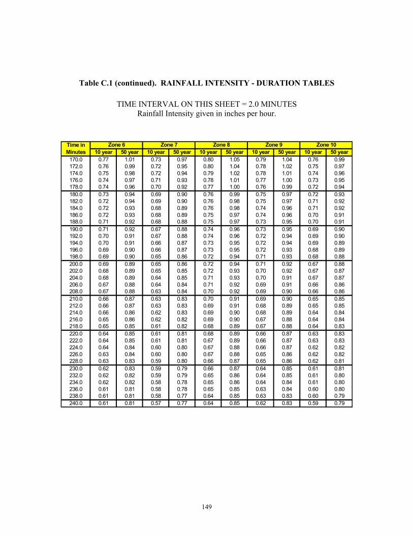
149

Table C.1 (continued). RAINFALL INTENSITY - DURATION TABLES

TIME INTERVAL ON THIS SHEET = 2.0 MINUTES Rainfall Intensity given in inches per hour.

10 year 50 year 10 year 50 year 10 year 50 year 10 year 50 year 10 year 50 year170.0 0.77 1.01 0.73 0.97 0.80 1.05 0.79 1.04 0.76 0.99172.0 0.76 0.99 0.72 0.95 0.80 1.04 0.78 1.02 0.75 0.97174.0 0.75 0.98 0.72 0.94 0.79 1.02 0.78 1.01 0.74 0.96176.0 0.74 0.97 0.71 0.93 0.78 1.01 0.77 1.00 0.73 0.95178.0 0.74 0.96 0.70 0.92 0.77 1.00 0.76 0.99 0.72 0.94180.0 0.73 0.94 0.69 0.90 0.76 0.99 0.75 0.97 0.72 0.93182.0 0.72 0.94 0.69 0.90 0.76 0.98 0.75 0.97 0.71 0.92184.0 0.72 0.93 0.68 0.89 0.76 0.98 0.74 0.96 0.71 0.92186.0 0.72 0.93 0.68 0.89 0.75 0.97 0.74 0.96 0.70 0.91188.0 0.71 0.92 0.68 0.88 0.75 0.97 0.73 0.95 0.70 0.91190.0 0.71 0.92 0.67 0.88 0.74 0.96 0.73 0.95 0.69 0.90192.0 0.70 0.91 0.67 0.88 0.74 0.96 0.72 0.94 0.69 0.90194.0 0.70 0.91 0.66 0.87 0.73 0.95 0.72 0.94 0.69 0.89196.0 0.69 0.90 0.66 0.87 0.73 0.95 0.72 0.93 0.68 0.89198.0 0.69 0.90 0.65 0.86 0.72 0.94 0.71 0.93 0.68 0.88200.0 0.69 0.89 0.65 0.86 0.72 0.94 0.71 0.92 0.67 0.88202.0 0.68 0.89 0.65 0.85 0.72 0.93 0.70 0.92 0.67 0.87204.0 0.68 0.89 0.64 0.85 0.71 0.93 0.70 0.91 0.67 0.87206.0 0.67 0.88 0.64 0.84 0.71 0.92 0.69 0.91 0.66 0.86208.0 0.67 0.88 0.63 0.84 0.70 0.92 0.69 0.90 0.66 0.86210.0 0.66 0.87 0.63 0.83 0.70 0.91 0.69 0.90 0.65 0.85212.0 0.66 0.87 0.63 0.83 0.69 0.91 0.68 0.89 0.65 0.85214.0 0.66 0.86 0.62 0.83 0.69 0.90 0.68 0.89 0.64 0.84216.0 0.65 0.86 0.62 0.82 0.69 0.90 0.67 0.88 0.64 0.84218.0 0.65 0.85 0.61 0.82 0.68 0.89 0.67 0.88 0.64 0.83220.0 0.64 0.85 0.61 0.81 0.68 0.89 0.66 0.87 0.63 0.83222.0 0.64 0.85 0.61 0.81 0.67 0.89 0.66 0.87 0.63 0.83224.0 0.64 0.84 0.60 0.80 0.67 0.88 0.66 0.87 0.62 0.82226.0 0.63 0.84 0.60 0.80 0.67 0.88 0.65 0.86 0.62 0.82228.0 0.63 0.83 0.59 0.80 0.66 0.87 0.65 0.86 0.62 0.81230.0 0.62 0.83 0.59 0.79 0.66 0.87 0.64 0.85 0.61 0.81232.0 0.62 0.82 0.59 0.79 0.65 0.86 0.64 0.85 0.61 0.80234.0 0.62 0.82 0.58 0.78 0.65 0.86 0.64 0.84 0.61 0.80236.0 0.61 0.81 0.58 0.78 0.65 0.85 0.63 0.84 0.60 0.80238.0 0.61 0.81 0.58 0.77 0.64 0.85 0.63 0.83 0.60 0.79240.0 0.61 0.81 0.57 0.77 0.64 0.85 0.62 0.83 0.59 0.79

Zone 6 Zone 7 Zone 8Time in Minutes

Zone 9 Zone 10

150

Table C.2. RAINFALL INTENSITY - DURATION METRIC TABLES

TIME INTERVAL ON THIS SHEET = 0.1 MINUTES Rainfall Intensity given in millimeters per hour.

10 year 50 year 10 year 50 year 10 year 50 year 10 year 50 year 10 year 50 year10.0 97.91 123.48 93.29 117.65 100.43 126.65 98.10 123.72 107.62 135.7210.1 97.49 122.98 92.89 117.17 100.00 126.13 97.68 123.21 107.16 135.1710.2 97.07 122.48 92.49 116.69 99.57 125.62 97.26 122.71 106.70 134.6210.3 96.66 121.98 92.09 116.22 99.14 125.12 96.84 122.21 106.24 134.0710.4 96.24 121.48 91.70 115.75 98.72 124.61 96.43 121.72 105.78 133.5310.5 95.83 120.99 91.30 115.28 98.29 124.10 96.01 121.22 105.33 132.9810.6 95.42 120.50 90.91 114.81 97.87 123.60 95.60 120.73 104.87 132.4410.7 95.01 120.01 90.52 114.34 97.45 123.10 95.19 120.24 104.42 131.9010.8 94.60 119.52 90.13 113.88 97.03 122.60 94.78 119.75 103.97 131.3710.9 94.19 119.04 89.74 113.42 96.62 122.11 94.37 119.26 103.53 130.8311.0 93.79 118.55 89.36 112.96 96.20 121.61 93.96 118.78 103.08 130.3011.1 93.38 118.07 88.97 112.50 95.79 121.12 93.56 118.29 102.64 129.7711.2 92.98 117.59 88.59 112.04 95.38 120.63 93.15 117.81 102.20 129.2511.3 92.58 117.12 88.21 111.58 94.97 120.14 92.75 117.33 101.76 128.7211.4 92.18 116.64 87.83 111.13 94.56 119.65 92.35 116.86 101.32 128.2011.5 91.79 116.17 87.45 110.68 94.16 119.17 91.96 116.38 100.88 127.6811.6 91.39 115.70 87.08 110.23 93.76 118.69 91.56 115.91 100.45 127.1611.7 91.00 115.23 86.70 109.78 93.35 118.20 91.17 115.44 100.02 126.6411.8 90.61 114.76 86.33 109.34 92.95 117.73 90.77 114.97 99.59 126.1311.9 90.22 114.29 85.96 108.89 92.55 117.25 90.38 114.50 99.16 125.6112.0 89.83 113.83 85.59 108.45 92.16 116.77 89.99 114.03 98.73 125.1012.1 89.45 113.37 85.22 108.01 91.76 116.30 89.61 113.57 98.31 124.6012.2 89.06 112.91 84.85 107.57 91.37 115.83 89.22 113.11 97.88 124.0912.3 88.68 112.45 84.49 107.13 90.98 115.36 88.84 112.65 97.46 123.5912.4 88.30 111.99 84.12 106.70 90.59 114.89 88.46 112.19 97.04 123.0812.5 87.92 111.54 83.76 106.26 90.20 114.43 88.07 111.73 96.63 122.5812.6 87.54 111.09 83.40 105.83 89.81 113.97 87.70 111.28 96.21 122.0912.7 87.17 110.63 83.04 105.40 89.43 113.50 87.32 110.83 95.80 121.5912.8 86.79 110.19 82.69 104.98 89.04 113.04 86.94 110.38 95.38 121.0912.9 86.42 109.74 82.33 104.55 88.66 112.59 86.57 109.93 94.97 120.6013.0 86.05 109.29 81.98 104.12 88.28 112.13 86.20 109.48 94.57 120.1113.1 85.68 108.85 81.62 103.70 87.90 111.68 85.82 109.04 94.16 119.6213.2 85.31 108.41 81.27 103.28 87.53 111.22 85.45 108.59 93.75 119.1413.3 84.94 107.97 80.92 102.86 87.15 110.77 85.09 108.15 93.35 118.6513.4 84.58 107.53 80.58 102.44 86.78 110.33 84.72 107.71 92.95 118.1713.5 84.21 107.09 80.23 102.03 86.40 109.88 84.36 107.27 92.55 117.6913.6 83.85 106.66 79.88 101.61 86.03 109.43 83.99 106.84 92.15 117.2113.7 83.49 106.22 79.54 101.20 85.67 108.99 83.63 106.40 91.75 116.7413.8 83.13 105.79 79.20 100.79 85.30 108.55 83.27 105.97 91.36 116.2613.9 82.78 105.36 78.86 100.38 84.93 108.11 82.91 105.54 90.97 115.79

Zone 5Zone 4Time in Minutes

Zone 1 Zone 2 Zone 3

151

Table C.2 (continued). RAINFALL INTENSITY - DURATION METRIC TABLES

TIME INTERVAL ON THIS SHEET = 0.1 MINUTES Rainfall Intensity given in millimeters per hour.

10 year 50 year 10 year 50 year 10 year 50 year 10 year 50 year 10 year 50 year14.0 82.42 104.94 78.52 99.97 84.57 107.67 82.56 105.11 90.58 115.3214.1 82.07 104.51 78.18 99.56 84.21 107.24 82.20 104.68 90.19 114.8514.2 81.71 104.09 77.85 99.16 83.84 106.80 81.85 104.26 89.80 114.3914.3 81.36 103.66 77.51 98.76 83.48 106.37 81.49 103.83 89.41 113.9214.4 81.01 103.24 77.18 98.36 83.13 105.94 81.14 103.41 89.03 113.4614.5 80.66 102.82 76.85 97.96 82.77 105.51 80.79 102.99 88.64 113.0014.6 80.32 102.41 76.52 97.56 82.42 105.08 80.45 102.57 88.26 112.5414.7 79.97 101.99 76.19 97.16 82.06 104.66 80.10 102.15 87.88 112.0814.8 79.63 101.58 75.86 96.77 81.71 104.23 79.76 101.74 87.51 111.6214.9 79.29 101.16 75.53 96.37 81.36 103.81 79.41 101.32 87.13 111.1715.0 78.95 100.75 75.21 95.98 81.01 103.39 79.07 100.91 86.75 110.7215.1 78.75 100.52 75.02 95.76 80.81 103.15 78.88 100.68 86.54 110.4615.2 78.56 100.29 74.84 95.54 80.61 102.91 78.68 100.45 86.33 110.2115.3 78.37 100.06 74.66 95.32 80.42 102.67 78.49 100.21 86.12 109.9515.4 78.18 99.83 74.48 95.10 80.22 102.43 78.30 99.98 85.91 109.7015.5 77.99 99.60 74.29 94.88 80.02 102.20 78.11 99.75 85.70 109.4515.6 77.80 99.37 74.11 94.66 79.83 101.96 77.92 99.52 85.49 109.1915.7 77.61 99.14 73.93 94.44 79.63 101.72 77.73 99.29 85.28 108.9415.8 77.42 98.91 73.75 94.22 79.44 101.49 77.54 99.06 85.08 108.6915.9 77.23 98.68 73.57 94.00 79.24 101.25 77.35 98.83 84.87 108.4416.0 77.05 98.46 73.39 93.79 79.05 101.02 77.16 98.61 84.66 108.1916.1 76.86 98.23 73.21 93.57 78.85 100.78 76.97 98.38 84.46 107.9416.2 76.67 98.00 73.03 93.35 78.66 100.55 76.79 98.15 84.25 107.6916.3 76.48 97.78 72.85 93.14 78.47 100.31 76.60 97.92 84.04 107.4416.4 76.30 97.55 72.68 92.92 78.28 100.08 76.41 97.70 83.84 107.1916.5 76.11 97.33 72.50 92.71 78.08 99.85 76.23 97.47 83.64 106.9516.6 75.93 97.10 72.32 92.49 77.89 99.62 76.04 97.25 83.43 106.7016.7 75.74 96.88 72.14 92.28 77.70 99.39 75.85 97.02 83.23 106.4516.8 75.56 96.66 71.97 92.06 77.51 99.16 75.67 96.80 83.02 106.2116.9 75.37 96.43 71.79 91.85 77.32 98.93 75.48 96.57 82.82 105.9617.0 75.19 96.21 71.62 91.64 77.13 98.70 75.30 96.35 82.62 105.7217.1 75.01 95.99 71.44 91.43 76.94 98.47 75.12 96.13 82.42 105.4717.2 74.83 95.77 71.27 91.21 76.76 98.24 74.93 95.91 82.22 105.2317.3 74.64 95.55 71.09 91.00 76.57 98.01 74.75 95.69 82.02 104.9917.4 74.46 95.33 70.92 90.79 76.38 97.78 74.57 95.46 81.82 104.7517.5 74.28 95.11 70.75 90.58 76.19 97.56 74.39 95.24 81.62 104.5017.6 74.10 94.89 70.57 90.37 76.01 97.33 74.20 95.02 81.42 104.2617.7 73.92 94.67 70.40 90.16 75.82 97.10 74.02 94.80 81.22 104.0217.8 73.74 94.45 70.23 89.96 75.63 96.88 73.84 94.59 81.02 103.7817.9 73.56 94.23 70.06 89.75 75.45 96.65 73.66 94.37 80.83 103.54

Zone 5Zone 4Time in Minutes

Zone 1 Zone 2 Zone 3

152

Table C.2 (continued). RAINFALL INTENSITY - DURATION METRIC TABLES

TIME INTERVAL ON THIS SHEET = 0.1 MINUTES Rainfall Intensity given in millimeters per hour.

10 year 50 year 10 year 50 year 10 year 50 year 10 year 50 year 10 year 50 year18.0 73.38 94.02 69.89 89.54 75.26 96.43 73.48 94.15 80.63 103.3018.1 73.20 93.80 69.72 89.33 75.08 96.21 73.30 93.93 80.43 103.0718.2 73.02 93.59 69.54 89.13 74.90 95.98 73.13 93.72 80.24 102.8318.3 72.85 93.37 69.37 88.92 74.71 95.76 72.95 93.50 80.04 102.5918.4 72.67 93.15 69.21 88.71 74.53 95.54 72.77 93.28 79.84 102.3518.5 72.49 92.94 69.04 88.51 74.35 95.32 72.59 93.07 79.65 102.1218.6 72.32 92.73 68.87 88.30 74.16 95.10 72.41 92.85 79.46 101.8818.7 72.14 92.51 68.70 88.10 73.98 94.88 72.24 92.64 79.26 101.6518.8 71.96 92.30 68.53 87.90 73.80 94.66 72.06 92.42 79.07 101.4118.9 71.79 92.09 68.36 87.69 73.62 94.44 71.89 92.21 78.88 101.1819.0 71.61 91.87 68.20 87.49 73.44 94.22 71.71 92.00 78.68 100.9419.1 71.44 91.66 68.03 87.29 73.26 94.00 71.54 91.79 78.49 100.7119.2 71.27 91.45 67.86 87.09 73.08 93.78 71.36 91.57 78.30 100.4819.3 71.09 91.24 67.70 86.88 72.90 93.56 71.19 91.36 78.11 100.2519.4 70.92 91.03 67.53 86.68 72.72 93.35 71.01 91.15 77.92 100.0219.5 70.75 90.82 67.37 86.48 72.54 93.13 70.84 90.94 77.73 99.7819.6 70.57 90.61 67.20 86.28 72.37 92.91 70.67 90.73 77.54 99.5519.7 70.40 90.40 67.04 86.08 72.19 92.70 70.49 90.52 77.35 99.3219.8 70.23 90.19 66.88 85.88 72.01 92.48 70.32 90.31 77.16 99.1019.9 70.06 89.99 66.71 85.69 71.84 92.27 70.15 90.10 76.97 98.8720.0 69.89 89.78 66.55 85.49 71.66 92.05 69.98 89.89 76.79 98.6420.1 69.72 89.57 66.39 85.29 71.49 91.84 69.81 89.69 76.60 98.4120.2 69.55 89.37 66.22 85.09 71.31 91.63 69.64 89.48 76.41 98.1820.3 69.38 89.16 66.06 84.90 71.14 91.41 69.47 89.27 76.23 97.9620.4 69.21 88.96 65.90 84.70 70.96 91.20 69.30 89.07 76.04 97.7320.5 69.04 88.75 65.74 84.50 70.79 90.99 69.13 88.86 75.85 97.5120.6 68.88 88.55 65.58 84.31 70.61 90.78 68.96 88.66 75.67 97.2820.7 68.71 88.34 65.42 84.11 70.44 90.57 68.79 88.45 75.49 97.0620.8 68.54 88.14 65.26 83.92 70.27 90.36 68.63 88.25 75.30 96.8320.9 68.37 87.94 65.10 83.72 70.10 90.15 68.46 88.04 75.12 96.6121.0 68.21 87.73 64.94 83.53 69.92 89.94 68.29 87.84 74.93 96.3821.1 68.04 87.53 64.78 83.34 69.75 89.73 68.12 87.64 74.75 96.1621.2 67.88 87.33 64.62 83.14 69.58 89.52 67.96 87.43 74.57 95.9421.3 67.71 87.13 64.47 82.95 69.41 89.32 67.79 87.23 74.39 95.7221.4 67.55 86.93 64.31 82.76 69.24 89.11 67.63 87.03 74.21 95.5021.5 67.38 86.73 64.15 82.57 69.07 88.90 67.46 86.83 74.03 95.2821.6 67.22 86.53 63.99 82.38 68.90 88.70 67.30 86.63 73.85 95.0621.7 67.05 86.33 63.84 82.19 68.73 88.49 67.13 86.43 73.66 94.8421.8 66.89 86.13 63.68 82.00 68.57 88.28 66.97 86.23 73.49 94.6221.9 66.73 85.93 63.53 81.81 68.40 88.08 66.81 86.03 73.31 94.40

Zone 5Time in Minutes

Zone 1 Zone 2 Zone 3 Zone 4

153

Table C.2 (continued). RAINFALL INTENSITY - DURATION METRIC TABLES

TIME INTERVAL ON THIS SHEET = 0.1 MINUTES Rainfall Intensity given in millimeters per hour.

10 year 50 year 10 year 50 year 10 year 50 year 10 year 50 year 10 year 50 year22.0 66.57 85.73 63.37 81.62 68.23 87.88 66.64 85.83 73.13 94.1822.1 66.40 85.53 63.22 81.43 68.06 87.67 66.48 85.63 72.95 93.9722.2 66.24 85.34 63.06 81.24 67.90 87.47 66.32 85.44 72.77 93.7522.3 66.08 85.14 62.91 81.05 67.73 87.27 66.16 85.24 72.59 93.5322.4 65.92 84.94 62.75 80.87 67.56 87.06 66.00 85.04 72.42 93.3222.5 65.76 84.75 62.60 80.68 67.40 86.86 65.83 84.85 72.24 93.1022.6 65.60 84.55 62.45 80.49 67.23 86.66 65.67 84.65 72.06 92.8922.7 65.44 84.36 62.30 80.31 67.07 86.46 65.51 84.45 71.89 92.6722.8 65.28 84.16 62.14 80.12 66.90 86.26 65.35 84.26 71.71 92.4622.9 65.12 83.97 61.99 79.93 66.74 86.06 65.19 84.06 71.54 92.2423.0 64.96 83.78 61.84 79.75 66.58 85.86 65.04 83.87 71.36 92.0323.1 64.81 83.58 61.69 79.57 66.41 85.66 64.88 83.68 71.19 91.8223.2 64.65 83.39 61.54 79.38 66.25 85.46 64.72 83.48 71.02 91.6123.3 64.49 83.20 61.39 79.20 66.09 85.26 64.56 83.29 70.84 91.4023.4 64.33 83.01 61.24 79.01 65.93 85.06 64.40 83.10 70.67 91.1923.5 64.18 82.82 61.09 78.83 65.77 84.87 64.25 82.91 70.50 90.9723.6 64.02 82.63 60.94 78.65 65.60 84.67 64.09 82.71 70.33 90.7623.7 63.86 82.44 60.79 78.47 65.44 84.47 63.93 82.52 70.15 90.5623.8 63.71 82.25 60.64 78.29 65.28 84.28 63.78 82.33 69.98 90.3523.9 63.55 82.06 60.49 78.10 65.12 84.08 63.62 82.14 69.81 90.1424.0 63.40 81.87 60.35 77.92 64.96 83.89 63.47 81.95 69.64 89.9324.1 63.25 81.68 60.20 77.74 64.80 83.69 63.31 81.76 69.47 89.7224.2 63.09 81.49 60.05 77.56 64.65 83.50 63.16 81.58 69.30 89.5124.3 62.94 81.30 59.90 77.38 64.49 83.30 63.00 81.39 69.13 89.3124.4 62.78 81.12 59.76 77.21 64.33 83.11 62.85 81.20 68.97 89.1024.5 62.63 80.93 59.61 77.03 64.17 82.92 62.70 81.01 68.80 88.9024.6 62.48 80.74 59.47 76.85 64.01 82.73 62.54 80.82 68.63 88.6924.7 62.33 80.56 59.32 76.67 63.86 82.53 62.39 80.64 68.46 88.4924.8 62.18 80.37 59.18 76.49 63.70 82.34 62.24 80.45 68.30 88.2824.9 62.02 80.19 59.03 76.32 63.55 82.15 62.09 80.27 68.13 88.0825.0 61.87 80.00 58.89 76.14 63.39 81.96 61.93 80.08 67.96 87.8825.1 61.72 79.82 58.74 75.96 63.23 81.77 61.78 79.90 67.80 87.6725.2 61.57 79.63 58.60 75.79 63.08 81.58 61.63 79.71 67.63 87.4725.3 61.42 79.45 58.46 75.61 62.92 81.39 61.48 79.53 67.47 87.2725.4 61.27 79.27 58.31 75.44 62.77 81.20 61.33 79.34 67.30 87.0725.5 61.12 79.08 58.17 75.26 62.62 81.01 61.18 79.16 67.14 86.8725.6 60.98 78.90 58.03 75.09 62.46 80.83 61.03 78.98 66.98 86.6725.7 60.83 78.72 57.89 74.92 62.31 80.64 60.88 78.79 66.81 86.4725.8 60.68 78.54 57.75 74.74 62.16 80.45 60.74 78.61 66.65 86.2725.9 60.53 78.36 57.61 74.57 62.01 80.27 60.59 78.43 66.49 86.07

Zone 5Zone 4Time in Minutes

Zone 1 Zone 2 Zone 3

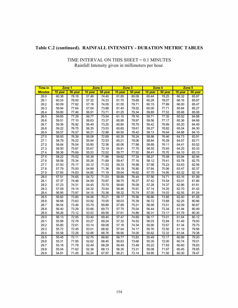
154

Table C.2 (continued). RAINFALL INTENSITY - DURATION METRIC TABLES

TIME INTERVAL ON THIS SHEET = 0.1 MINUTES Rainfall Intensity given in millimeters per hour.

10 year 50 year 10 year 50 year 10 year 50 year 10 year 50 year 10 year 50 year26.0 60.38 78.18 57.46 74.40 61.85 80.08 60.44 78.25 66.32 85.8726.1 60.24 78.00 57.32 74.23 61.70 79.89 60.29 78.07 66.16 85.6726.2 60.09 77.82 57.18 74.05 61.55 79.71 60.15 77.89 66.00 85.4726.3 59.94 77.64 57.04 73.88 61.40 79.52 60.00 77.71 65.84 85.2726.4 59.80 77.46 56.91 73.71 61.25 79.34 59.85 77.53 65.68 85.0826.5 59.65 77.28 56.77 73.54 61.10 79.16 59.71 77.35 65.52 84.8826.6 59.51 77.10 56.63 73.37 60.95 78.97 59.56 77.17 65.36 84.6926.7 59.36 76.92 56.49 73.20 60.80 78.79 59.42 76.99 65.20 84.4926.8 59.22 76.75 56.35 73.03 60.65 78.61 59.27 76.82 65.04 84.3026.9 59.07 76.57 56.21 72.86 60.50 78.42 59.13 76.64 64.88 84.1027.0 58.93 76.39 56.08 72.69 60.35 78.24 58.98 76.46 64.73 83.9127.1 58.79 76.22 55.94 72.53 60.21 78.06 58.84 76.28 64.57 83.7127.2 58.64 76.04 55.80 72.36 60.06 77.88 58.69 76.11 64.41 83.5227.3 58.50 75.87 55.67 72.19 59.91 77.70 58.55 75.93 64.25 83.3327.4 58.36 75.69 55.53 72.02 59.77 77.52 58.41 75.76 64.10 83.1327.5 58.22 75.52 55.39 71.86 59.62 77.34 58.27 75.58 63.94 82.9427.6 58.08 75.34 55.26 71.69 59.47 77.16 58.12 75.41 63.78 82.7527.7 57.93 75.17 55.12 71.53 59.33 76.98 57.98 75.23 63.63 82.5627.8 57.79 75.00 54.99 71.36 59.18 76.80 57.84 75.06 63.47 82.3727.9 57.65 74.83 54.85 71.19 59.04 76.62 57.70 74.89 63.32 82.1828.0 57.51 74.65 54.72 71.03 58.89 76.44 57.56 74.71 63.16 81.9928.1 57.37 74.48 54.59 70.87 58.75 76.27 57.42 74.54 63.01 81.8028.2 57.23 74.31 54.45 70.70 58.60 76.09 57.28 74.37 62.86 81.6128.3 57.09 74.14 54.32 70.54 58.46 75.91 57.14 74.20 62.70 81.4228.4 56.95 73.97 54.19 70.38 58.32 75.74 57.00 74.03 62.55 81.2428.5 56.82 73.80 54.06 70.21 58.17 75.56 56.86 73.85 62.40 81.0528.6 56.68 73.63 53.92 70.05 58.03 75.39 56.72 73.68 62.25 80.8628.7 56.54 73.46 53.79 69.89 57.89 75.21 56.58 73.51 62.09 80.6728.8 56.40 73.29 53.66 69.73 57.75 75.04 56.44 73.34 61.94 80.4928.9 56.26 73.12 53.53 69.56 57.61 74.86 56.31 73.17 61.79 80.3029.0 56.13 72.95 53.40 69.40 57.47 74.69 56.17 73.01 61.64 80.1229.1 55.99 72.78 53.27 69.24 57.32 74.52 56.03 72.84 61.49 79.9329.2 55.85 72.61 53.14 69.08 57.18 74.34 55.90 72.67 61.34 79.7529.3 55.72 72.45 53.01 68.92 57.04 74.17 55.76 72.50 61.19 79.5629.4 55.58 72.28 52.88 68.76 56.90 74.00 55.62 72.33 61.04 79.3829.5 55.45 72.11 52.75 68.60 56.77 73.83 55.49 72.17 60.89 79.2029.6 55.31 71.95 52.62 68.45 56.63 73.66 55.35 72.00 60.74 79.0129.7 55.18 71.78 52.49 68.29 56.49 73.49 55.22 71.83 60.60 78.8329.8 55.04 71.62 52.36 68.13 56.35 73.31 55.08 71.67 60.45 78.6529.9 54.91 71.45 52.24 67.97 56.21 73.14 54.95 71.50 60.30 78.47

Zone 5Time in Minutes

Zone 1 Zone 2 Zone 3 Zone 4

155

Table C.2 (continued). RAINFALL INTENSITY - DURATION METRIC TABLES

TIME INTERVAL ON THIS SHEET = 0.2 MINUTES Rainfall Intensity given in millimeters per hour.

10 year 50 year 10 year 50 year 10 year 50 year 10 year 50 year 10 year 50 year30.0 54.78 71.29 52.11 67.82 56.07 72.98 54.81 71.34 60.15 78.2930.2 54.65 71.14 51.99 67.69 55.94 72.83 54.69 71.20 60.01 78.1430.4 54.53 71.00 51.87 67.56 55.81 72.69 54.56 71.06 59.88 77.9930.6 54.40 70.85 51.75 67.44 55.68 72.54 54.43 70.92 59.74 77.8430.8 54.28 70.71 51.63 67.31 55.54 72.40 54.31 70.78 59.60 77.6931.0 54.15 70.57 51.51 67.19 55.41 72.25 54.18 70.64 59.46 77.5431.2 54.03 70.42 51.40 67.06 55.28 72.11 54.05 70.50 59.32 77.3931.4 53.91 70.28 51.28 66.94 55.15 71.97 53.93 70.36 59.18 77.2431.6 53.78 70.14 51.16 66.81 55.02 71.83 53.80 70.22 59.05 77.0931.8 53.66 69.99 51.04 66.69 54.89 71.68 53.68 70.08 58.91 76.9432.0 53.54 69.85 50.93 66.57 54.76 71.54 53.55 69.94 58.77 76.7932.2 53.42 69.71 50.81 66.44 54.63 71.40 53.43 69.80 58.64 76.6532.4 53.29 69.57 50.69 66.32 54.50 71.26 53.30 69.67 58.50 76.5032.6 53.17 69.43 50.58 66.20 54.37 71.12 53.18 69.53 58.36 76.3532.8 53.05 69.29 50.46 66.07 54.24 70.98 53.05 69.39 58.23 76.2033.0 52.93 69.15 50.34 65.95 54.11 70.84 52.93 69.26 58.09 76.0633.2 52.81 69.01 50.23 65.83 53.99 70.70 52.81 69.12 57.96 75.9133.4 52.69 68.87 50.11 65.71 53.86 70.55 52.69 68.98 57.82 75.7733.6 52.57 68.73 50.00 65.58 53.73 70.42 52.56 68.85 57.69 75.6233.8 52.45 68.59 49.88 65.46 53.60 70.28 52.44 68.71 57.55 75.4734.0 52.33 68.45 49.77 65.34 53.48 70.14 52.32 68.57 57.42 75.3334.2 52.21 68.31 49.66 65.22 53.35 70.00 52.20 68.44 57.29 75.1834.4 52.09 68.17 49.54 65.10 53.22 69.86 52.07 68.30 57.15 75.0434.6 51.97 68.03 49.43 64.98 53.10 69.72 51.95 68.17 57.02 74.9034.8 51.85 67.89 49.32 64.86 52.97 69.58 51.83 68.04 56.89 74.7535.0 51.73 67.75 49.20 64.74 52.85 69.44 51.71 67.90 56.76 74.6135.2 51.61 67.62 49.09 64.62 52.72 69.31 51.59 67.77 56.63 74.4635.4 51.50 67.48 48.98 64.50 52.60 69.17 51.47 67.63 56.49 74.3235.6 51.38 67.34 48.86 64.38 52.47 69.03 51.35 67.50 56.36 74.1835.8 51.26 67.21 48.75 64.26 52.35 68.90 51.23 67.37 56.23 74.0436.0 51.14 67.07 48.64 64.14 52.23 68.76 51.11 67.23 56.10 73.8936.2 51.03 66.93 48.53 64.02 52.10 68.62 50.99 67.10 55.97 73.7536.4 50.91 66.80 48.42 63.90 51.98 68.49 50.88 66.97 55.84 73.6136.6 50.79 66.66 48.31 63.78 51.86 68.35 50.76 66.84 55.71 73.4736.8 50.68 66.53 48.20 63.66 51.73 68.22 50.64 66.71 55.58 73.3337.0 50.56 66.39 48.09 63.54 51.61 68.08 50.52 66.57 55.45 73.1837.2 50.45 66.26 47.98 63.43 51.49 67.94 50.40 66.44 55.32 73.0437.4 50.33 66.12 47.87 63.31 51.37 67.81 50.29 66.31 55.20 72.9037.6 50.22 65.99 47.76 63.19 51.24 67.68 50.17 66.18 55.07 72.7637.8 50.10 65.85 47.65 63.07 51.12 67.54 50.05 66.05 54.94 72.62

Zone 5Zone 4Time in Minutes

Zone 1 Zone 2 Zone 3

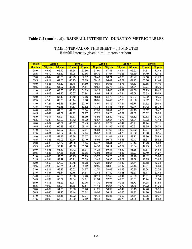
156

Table C.2 (continued). RAINFALL INTENSITY - DURATION METRIC TABLES

TIME INTERVAL ON THIS SHEET = 0.5 MINUTES Rainfall Intensity given in millimeters per hour.

10 year 50 year 10 year 50 year 10 year 50 year 10 year 50 year 10 year 50 year38.0 49.99 65.72 47.54 62.96 51.00 67.41 49.94 65.92 54.81 72.4838.5 49.70 65.39 47.26 62.66 50.70 67.07 49.65 65.60 54.49 72.1439.0 49.42 65.06 46.99 62.37 50.40 66.74 49.36 65.27 54.18 71.7939.5 49.14 64.73 46.73 62.09 50.10 66.41 49.07 64.95 53.86 71.4440.0 48.86 64.40 46.46 61.80 49.81 66.08 48.78 64.63 53.55 71.1040.5 48.58 64.07 46.19 61.51 49.51 65.76 48.50 64.31 53.24 70.7641.0 48.30 63.75 45.93 61.23 49.22 65.43 48.22 64.00 52.93 70.4241.5 48.03 63.42 45.67 60.94 48.93 65.11 47.94 63.68 52.63 70.0842.0 47.75 63.10 45.40 60.66 48.64 64.79 47.66 63.37 52.32 69.7542.5 47.48 62.78 45.14 60.38 48.35 64.47 47.38 63.06 52.02 69.4143.0 47.21 62.46 44.89 60.10 48.07 64.15 47.11 62.74 51.72 69.0843.5 46.94 62.15 44.63 59.82 47.78 63.83 46.84 62.44 51.42 68.7544.0 46.67 61.83 44.37 59.54 47.50 63.51 46.56 62.13 51.12 68.4244.5 46.41 61.52 44.12 59.27 47.22 63.20 46.29 61.82 50.82 68.0945.0 46.14 61.21 43.87 58.99 46.94 62.89 46.02 61.52 50.53 67.7645.5 45.88 60.90 43.62 58.72 46.67 62.57 45.76 61.21 50.23 67.4346.0 45.62 60.59 43.37 58.45 46.39 62.27 45.49 60.91 49.94 67.1146.5 45.36 60.28 43.12 58.18 46.12 61.96 45.23 60.61 49.65 66.7947.0 45.10 59.97 42.87 57.91 45.84 61.65 44.96 60.32 49.37 66.4747.5 44.84 59.67 42.63 57.64 45.57 61.35 44.70 60.02 49.08 66.1548.0 44.59 59.37 42.38 57.37 45.30 61.04 44.44 59.72 48.80 65.8348.5 44.33 59.07 42.14 57.10 45.04 60.74 44.18 59.43 48.51 65.5249.0 44.08 58.77 41.90 56.84 44.77 60.44 43.93 59.14 48.23 65.2049.5 43.83 58.47 41.66 56.58 44.50 60.14 43.67 58.84 47.95 64.8950.0 43.58 58.17 41.42 56.31 44.24 59.84 43.42 58.55 47.67 64.5850.5 43.33 57.88 41.18 56.05 43.98 59.55 43.17 58.27 47.40 64.2751.0 43.08 57.58 40.95 55.79 43.72 59.25 42.92 57.98 47.12 63.9651.5 42.84 57.29 40.71 55.53 43.46 58.96 42.67 57.69 46.85 63.6552.0 42.59 57.00 40.48 55.28 43.21 58.67 42.42 57.41 46.58 63.3452.5 42.35 56.71 40.25 55.02 42.95 58.38 42.17 57.13 46.31 63.0453.0 42.11 56.43 40.02 54.77 42.70 58.09 41.93 56.85 46.04 62.7453.5 41.87 56.14 39.79 54.51 42.44 57.80 41.68 56.57 45.77 62.4454.0 41.63 55.86 39.56 54.26 42.19 57.52 41.44 56.29 45.51 62.1454.5 41.39 55.57 39.34 54.01 41.94 57.23 41.20 56.01 45.24 61.8455.0 41.15 55.29 39.11 53.76 41.70 56.95 40.96 55.73 44.98 61.5455.5 40.92 55.01 38.89 53.51 41.45 56.67 40.72 55.46 44.72 61.2556.0 40.69 54.73 38.66 53.26 41.21 56.39 40.49 55.19 44.46 60.9556.5 40.46 54.45 38.44 53.01 40.96 56.11 40.25 54.92 44.20 60.6657.0 40.22 54.18 38.22 52.77 40.72 55.83 40.02 54.64 43.95 60.3757.5 39.99 53.90 38.00 52.52 40.48 55.55 39.78 54.38 43.69 60.08

Zone 5Time in Minutes

Zone 1 Zone 2 Zone 3 Zone 4

157

Table C.2 (continued). RAINFALL INTENSITY - DURATION METRIC TABLES

TIME INTERVAL ON THIS SHEET = 1.0 MINUTES Rainfall Intensity given in millimeters per hour.

10 year 50 year 10 year 50 year 10 year 50 year 10 year 50 year 10 year 50 year58.0 39.77 53.63 37.79 52.28 40.24 55.28 39.55 54.11 43.44 59.7959.0 39.31 53.09 37.36 51.80 39.77 54.73 39.10 53.58 42.94 59.2260.0 38.87 52.55 36.93 51.32 39.30 54.19 38.64 53.05 42.44 58.6561.0 38.52 52.11 36.62 50.90 38.97 53.76 38.30 52.61 42.08 58.1762.0 38.18 51.67 36.31 50.48 38.64 53.32 37.97 52.17 41.73 57.6963.0 37.85 51.24 36.00 50.07 38.32 52.89 37.64 51.73 41.38 57.2164.0 37.51 50.81 35.70 49.67 38.00 52.47 37.31 51.30 41.03 56.7465.0 37.18 50.38 35.40 49.26 37.68 52.05 36.98 50.87 40.68 56.2766.0 36.85 49.96 35.10 48.86 37.37 51.63 36.66 50.45 40.34 55.8167.0 36.53 49.54 34.80 48.46 37.05 51.21 36.34 50.03 40.00 55.3568.0 36.21 49.12 34.51 48.07 36.74 50.80 36.02 49.61 39.66 54.8969.0 35.89 48.71 34.22 47.68 36.44 50.39 35.70 49.20 39.33 54.4470.0 35.57 48.30 33.93 47.29 36.13 49.98 35.39 48.79 38.99 53.9971.0 35.26 47.90 33.64 46.90 35.83 49.58 35.08 48.38 38.67 53.5472.0 34.95 47.50 33.36 46.52 35.53 49.18 34.77 47.97 38.34 53.1073.0 34.64 47.10 33.08 46.14 35.23 48.79 34.47 47.57 38.02 52.6774.0 34.33 46.70 32.80 45.77 34.94 48.39 34.17 47.18 37.70 52.2375.0 34.03 46.31 32.52 45.39 34.64 48.00 33.87 46.78 37.38 51.8076.0 33.73 45.92 32.25 45.02 34.35 47.62 33.57 46.39 37.06 51.3777.0 33.43 45.54 31.98 44.66 34.07 47.24 33.28 46.01 36.75 50.9578.0 33.14 45.15 31.71 44.29 33.78 46.85 32.98 45.62 36.44 50.5379.0 32.84 44.77 31.44 43.93 33.50 46.48 32.70 45.24 36.13 50.1180.0 32.55 44.40 31.17 43.58 33.22 46.10 32.41 44.86 35.83 49.7081.0 32.27 44.03 30.91 43.22 32.94 45.73 32.13 44.49 35.53 49.2982.0 31.98 43.66 30.65 42.87 32.66 45.36 31.84 44.12 35.23 48.8883.0 31.70 43.29 30.39 42.52 32.39 45.00 31.57 43.75 34.93 48.4884.0 31.42 42.93 30.13 42.17 32.12 44.64 31.29 43.39 34.63 48.0885.0 31.14 42.57 29.88 41.83 31.85 44.28 31.01 43.02 34.34 47.6986.0 30.87 42.21 29.63 41.49 31.58 43.92 30.74 42.66 34.05 47.2987.0 30.60 41.86 29.38 41.15 31.32 43.57 30.47 42.31 33.77 46.9088.0 30.33 41.50 29.13 40.82 31.06 43.22 30.21 41.95 33.48 46.5289.0 30.06 41.16 28.88 40.49 30.80 42.87 29.94 41.60 33.20 46.1390.0 29.79 40.81 28.64 40.16 30.54 42.52 29.68 41.26 32.92 45.7591.0 29.53 40.47 28.40 39.83 30.29 42.18 29.42 40.91 32.64 45.3792.0 29.27 40.13 28.16 39.50 30.03 41.84 29.16 40.57 32.37 45.0093.0 29.01 39.79 27.92 39.18 29.78 41.51 28.91 40.23 32.09 44.6394.0 28.75 39.46 27.69 38.86 29.53 41.17 28.65 39.90 31.82 44.2695.0 28.50 39.13 27.45 38.55 29.28 40.84 28.40 39.56 31.55 43.9096.0 28.25 38.80 27.22 38.23 29.04 40.51 28.15 39.23 31.29 43.5397.0 28.00 38.47 26.99 37.92 28.80 40.19 27.91 38.91 31.02 43.1898.0 27.75 38.15 26.76 37.61 28.56 39.86 27.66 38.58 30.76 42.82

Zone 5Zone 4Time in Minutes

Zone 1 Zone 2 Zone 3

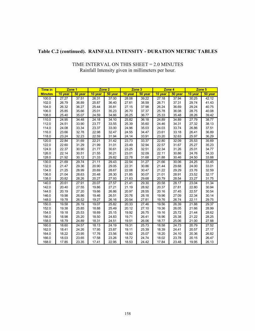
158

Table C.2 (continued). RAINFALL INTENSITY - DURATION METRIC TABLES

TIME INTERVAL ON THIS SHEET = 2.0 MINUTES Rainfall Intensity given in millimeters per hour.

10 year 50 year 10 year 50 year 10 year 50 year 10 year 50 year 10 year 50 year100.0 27.27 37.51 26.31 37.00 28.08 39.22 27.18 37.94 30.25 42.12102.0 26.79 36.89 25.87 36.40 27.61 38.59 26.71 37.31 29.74 41.43104.0 26.32 36.27 25.44 35.81 27.15 37.98 26.24 36.69 29.24 40.75106.0 25.85 35.66 25.01 35.23 26.70 37.37 25.78 36.08 28.75 40.08108.0 25.40 35.07 24.59 34.66 26.25 36.77 25.33 35.48 28.26 39.42110.0 24.95 34.48 24.18 34.10 25.82 36.18 24.89 34.89 27.79 38.77112.0 24.51 33.90 23.77 33.55 25.39 35.60 24.46 34.31 27.32 38.13114.0 24.08 33.34 23.37 33.00 24.96 35.03 24.03 33.74 26.86 37.51116.0 23.66 32.78 22.98 32.47 24.55 34.47 23.61 33.18 26.41 36.89118.0 23.24 32.23 22.59 31.94 24.14 33.91 23.20 32.63 25.97 36.29120.0 22.84 31.69 22.21 31.42 23.73 33.37 22.80 32.09 25.53 35.69122.0 22.60 31.29 21.99 31.01 23.49 32.94 22.57 31.67 25.27 35.23124.0 22.37 30.90 21.77 30.61 23.25 32.51 22.34 31.26 25.01 34.77126.0 22.14 30.51 21.55 30.21 23.01 32.09 22.11 30.86 24.76 34.33128.0 21.92 30.12 21.33 29.82 22.78 31.68 21.88 30.46 24.50 33.88130.0 21.69 29.74 21.11 29.43 22.54 31.27 21.66 30.06 24.25 33.45132.0 21.47 29.36 20.90 29.05 22.31 30.86 21.44 29.68 24.00 33.01134.0 21.25 28.99 20.69 28.67 22.08 30.47 21.22 29.29 23.76 32.59136.0 21.04 28.63 20.48 28.30 21.85 30.07 21.01 28.91 23.52 32.17138.0 20.82 28.26 20.27 27.93 21.63 29.68 20.79 28.54 23.27 31.75140.0 20.61 27.91 20.07 27.57 21.41 29.30 20.58 28.17 23.04 31.34142.0 20.40 27.55 19.86 27.21 21.19 28.92 20.37 27.81 22.80 30.94144.0 20.19 27.20 19.66 26.86 20.97 28.55 20.16 27.45 22.57 30.54146.0 19.98 26.86 19.46 26.51 20.76 28.18 19.96 27.09 22.34 30.14148.0 19.78 26.52 19.27 26.16 20.54 27.81 19.76 26.74 22.11 29.75150.0 19.58 26.19 19.07 25.82 20.33 27.46 19.56 26.39 21.88 29.37152.0 19.38 25.85 18.88 25.49 20.12 27.10 19.36 26.05 21.66 28.99154.0 19.18 25.53 18.69 25.15 19.92 26.75 19.16 25.72 21.44 28.62156.0 18.98 25.20 18.50 24.83 19.71 26.41 18.96 25.38 21.22 28.25158.0 18.79 24.89 18.31 24.51 19.51 26.06 18.77 25.06 21.00 27.88160.0 18.60 24.57 18.13 24.19 19.31 25.73 18.58 24.73 20.79 27.52162.0 18.41 24.26 17.95 23.87 19.11 25.39 18.39 24.41 20.57 27.17164.0 18.22 23.95 17.76 23.56 18.92 25.07 18.20 24.10 20.36 26.82166.0 18.03 23.65 17.58 23.26 18.72 24.74 18.02 23.78 20.15 26.47168.0 17.85 23.35 17.41 22.95 18.53 24.42 17.84 23.48 19.95 26.13

Zone 5Time in Minutes

Zone 1 Zone 2 Zone 3 Zone 4

159

Table C.2 (continued). RAINFALL INTENSITY - DURATION METRIC TABLES

TIME INTERVAL ON THIS SHEET = 2.0 MINUTES Rainfall Intensity given in millimeters per hour.

10 year 50 year 10 year 50 year 10 year 50 year 10 year 50 year 10 year 50 year170.0 17.67 23.06 17.23 22.65 18.34 24.11 17.65 23.17 19.74 25.79172.0 17.49 22.76 17.06 22.36 18.15 23.80 17.47 22.87 19.54 25.46174.0 17.31 22.48 16.88 22.07 17.96 23.49 17.30 22.58 19.34 25.13176.0 17.13 22.19 16.71 21.78 17.78 23.19 17.12 22.29 19.14 24.80178.0 16.96 21.91 16.55 21.50 17.60 22.89 16.95 22.00 18.95 24.48180.0 16.78 21.63 16.38 21.22 17.42 22.59 16.77 21.71 18.75 24.17182.0 16.68 21.52 16.28 21.11 17.31 22.48 16.67 21.60 18.64 24.05184.0 16.58 21.41 16.18 21.00 17.21 22.36 16.57 21.49 18.53 23.93186.0 16.48 21.30 16.08 20.90 17.10 22.25 16.47 21.38 18.42 23.81188.0 16.38 21.19 15.99 20.79 17.00 22.14 16.37 21.27 18.31 23.69190.0 16.28 21.08 15.89 20.68 16.89 22.02 16.27 21.16 18.20 23.57192.0 16.19 20.97 15.79 20.58 16.79 21.91 16.17 21.05 18.10 23.45194.0 16.09 20.86 15.70 20.47 16.69 21.80 16.07 20.94 17.99 23.33196.0 15.99 20.75 15.60 20.37 16.59 21.69 15.97 20.84 17.88 23.21198.0 15.90 20.65 15.51 20.27 16.48 21.58 15.87 20.73 17.78 23.10200.0 15.80 20.54 15.41 20.16 16.38 21.47 15.78 20.62 17.67 22.98202.0 15.70 20.43 15.32 20.06 16.28 21.36 15.68 20.52 17.57 22.86204.0 15.61 20.33 15.23 19.96 16.18 21.26 15.58 20.41 17.46 22.75206.0 15.52 20.22 15.13 19.86 16.09 21.15 15.49 20.31 17.36 22.64208.0 15.42 20.12 15.04 19.76 15.99 21.04 15.39 20.20 17.26 22.52210.0 15.33 20.01 14.95 19.65 15.89 20.93 15.30 20.10 17.15 22.41212.0 15.24 19.91 14.86 19.55 15.79 20.83 15.21 20.00 17.05 22.30214.0 15.15 19.81 14.77 19.45 15.70 20.72 15.11 19.89 16.95 22.18216.0 15.05 19.70 14.68 19.36 15.60 20.62 15.02 19.79 16.85 22.07218.0 14.96 19.60 14.59 19.26 15.51 20.51 14.93 19.69 16.75 21.96220.0 14.87 19.50 14.51 19.16 15.41 20.41 14.84 19.59 16.65 21.85222.0 14.78 19.40 14.42 19.06 15.32 20.31 14.75 19.49 16.55 21.74224.0 14.70 19.30 14.33 18.96 15.22 20.20 14.66 19.39 16.45 21.63226.0 14.61 19.20 14.24 18.87 15.13 20.10 14.57 19.29 16.36 21.52228.0 14.52 19.10 14.16 18.77 15.04 20.00 14.48 19.19 16.26 21.41230.0 14.43 19.00 14.07 18.68 14.95 19.90 14.39 19.09 16.16 21.31232.0 14.34 18.90 13.99 18.58 14.86 19.80 14.30 18.99 16.07 21.20234.0 14.26 18.81 13.90 18.49 14.77 19.70 14.21 18.90 15.97 21.09236.0 14.17 18.71 13.82 18.39 14.68 19.60 14.13 18.80 15.88 20.99238.0 14.09 18.61 13.73 18.30 14.59 19.50 14.04 18.70 15.78 20.88240.0 14.00 18.51 13.65 18.20 14.50 19.40 13.96 18.61 15.69 20.78

Zone 5Zone 4Time in Minutes

Zone 1 Zone 2 Zone 3

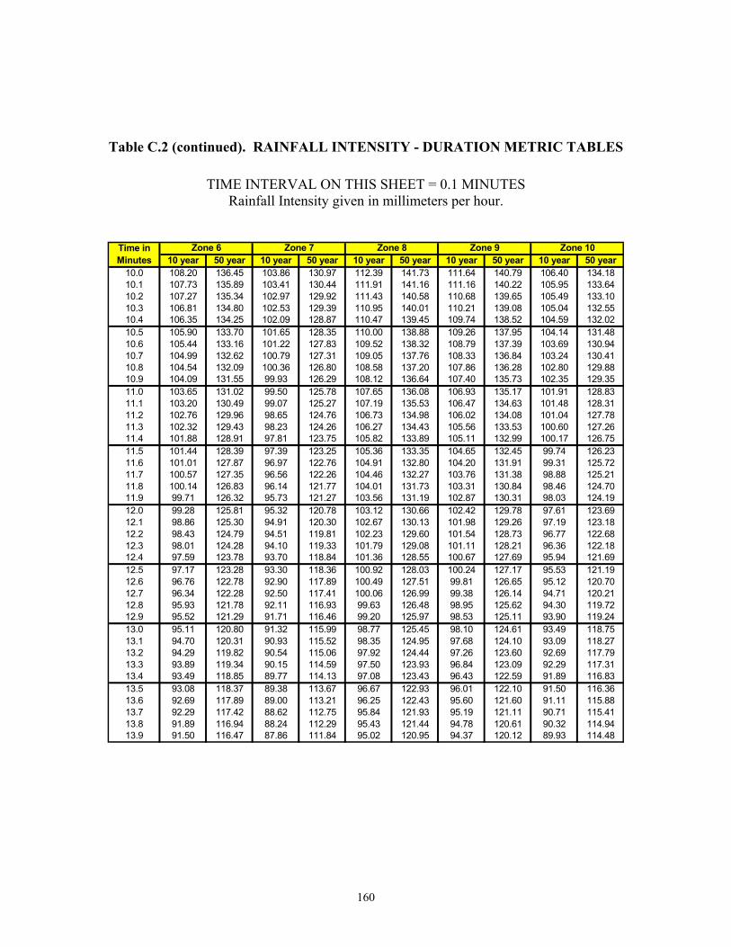
160

Table C.2 (continued). RAINFALL INTENSITY - DURATION METRIC TABLES

TIME INTERVAL ON THIS SHEET = 0.1 MINUTES Rainfall Intensity given in millimeters per hour.

10 year 50 year 10 year 50 year 10 year 50 year 10 year 50 year 10 year 50 year10.0 108.20 136.45 103.86 130.97 112.39 141.73 111.64 140.79 106.40 134.1810.1 107.73 135.89 103.41 130.44 111.91 141.16 111.16 140.22 105.95 133.6410.2 107.27 135.34 102.97 129.92 111.43 140.58 110.68 139.65 105.49 133.1010.3 106.81 134.80 102.53 129.39 110.95 140.01 110.21 139.08 105.04 132.5510.4 106.35 134.25 102.09 128.87 110.47 139.45 109.74 138.52 104.59 132.0210.5 105.90 133.70 101.65 128.35 110.00 138.88 109.26 137.95 104.14 131.4810.6 105.44 133.16 101.22 127.83 109.52 138.32 108.79 137.39 103.69 130.9410.7 104.99 132.62 100.79 127.31 109.05 137.76 108.33 136.84 103.24 130.4110.8 104.54 132.09 100.36 126.80 108.58 137.20 107.86 136.28 102.80 129.8810.9 104.09 131.55 99.93 126.29 108.12 136.64 107.40 135.73 102.35 129.3511.0 103.65 131.02 99.50 125.78 107.65 136.08 106.93 135.17 101.91 128.8311.1 103.20 130.49 99.07 125.27 107.19 135.53 106.47 134.63 101.48 128.3111.2 102.76 129.96 98.65 124.76 106.73 134.98 106.02 134.08 101.04 127.7811.3 102.32 129.43 98.23 124.26 106.27 134.43 105.56 133.53 100.60 127.2611.4 101.88 128.91 97.81 123.75 105.82 133.89 105.11 132.99 100.17 126.7511.5 101.44 128.39 97.39 123.25 105.36 133.35 104.65 132.45 99.74 126.2311.6 101.01 127.87 96.97 122.76 104.91 132.80 104.20 131.91 99.31 125.7211.7 100.57 127.35 96.56 122.26 104.46 132.27 103.76 131.38 98.88 125.2111.8 100.14 126.83 96.14 121.77 104.01 131.73 103.31 130.84 98.46 124.7011.9 99.71 126.32 95.73 121.27 103.56 131.19 102.87 130.31 98.03 124.1912.0 99.28 125.81 95.32 120.78 103.12 130.66 102.42 129.78 97.61 123.6912.1 98.86 125.30 94.91 120.30 102.67 130.13 101.98 129.26 97.19 123.1812.2 98.43 124.79 94.51 119.81 102.23 129.60 101.54 128.73 96.77 122.6812.3 98.01 124.28 94.10 119.33 101.79 129.08 101.11 128.21 96.36 122.1812.4 97.59 123.78 93.70 118.84 101.36 128.55 100.67 127.69 95.94 121.6912.5 97.17 123.28 93.30 118.36 100.92 128.03 100.24 127.17 95.53 121.1912.6 96.76 122.78 92.90 117.89 100.49 127.51 99.81 126.65 95.12 120.7012.7 96.34 122.28 92.50 117.41 100.06 126.99 99.38 126.14 94.71 120.2112.8 95.93 121.78 92.11 116.93 99.63 126.48 98.95 125.62 94.30 119.7212.9 95.52 121.29 91.71 116.46 99.20 125.97 98.53 125.11 93.90 119.2413.0 95.11 120.80 91.32 115.99 98.77 125.45 98.10 124.61 93.49 118.7513.1 94.70 120.31 90.93 115.52 98.35 124.95 97.68 124.10 93.09 118.2713.2 94.29 119.82 90.54 115.06 97.92 124.44 97.26 123.60 92.69 117.7913.3 93.89 119.34 90.15 114.59 97.50 123.93 96.84 123.09 92.29 117.3113.4 93.49 118.85 89.77 114.13 97.08 123.43 96.43 122.59 91.89 116.8313.5 93.08 118.37 89.38 113.67 96.67 122.93 96.01 122.10 91.50 116.3613.6 92.69 117.89 89.00 113.21 96.25 122.43 95.60 121.60 91.11 115.8813.7 92.29 117.42 88.62 112.75 95.84 121.93 95.19 121.11 90.71 115.4113.8 91.89 116.94 88.24 112.29 95.43 121.44 94.78 120.61 90.32 114.9413.9 91.50 116.47 87.86 111.84 95.02 120.95 94.37 120.12 89.93 114.48

Time in Minutes

Zone 9 Zone 10Zone 7 Zone 8Zone 6

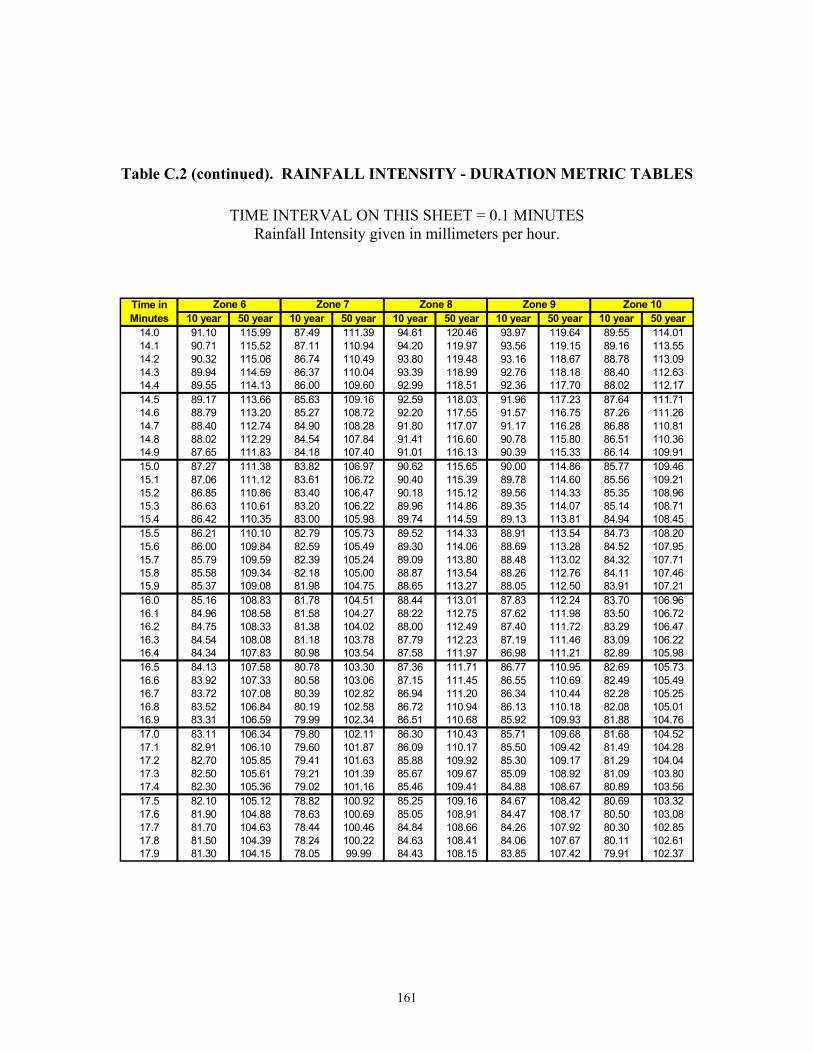
161

Table C.2 (continued). RAINFALL INTENSITY - DURATION METRIC TABLES

TIME INTERVAL ON THIS SHEET = 0.1 MINUTES Rainfall Intensity given in millimeters per hour.

10 year 50 year 10 year 50 year 10 year 50 year 10 year 50 year 10 year 50 year14.0 91.10 115.99 87.49 111.39 94.61 120.46 93.97 119.64 89.55 114.0114.1 90.71 115.52 87.11 110.94 94.20 119.97 93.56 119.15 89.16 113.5514.2 90.32 115.06 86.74 110.49 93.80 119.48 93.16 118.67 88.78 113.0914.3 89.94 114.59 86.37 110.04 93.39 118.99 92.76 118.18 88.40 112.6314.4 89.55 114.13 86.00 109.60 92.99 118.51 92.36 117.70 88.02 112.1714.5 89.17 113.66 85.63 109.16 92.59 118.03 91.96 117.23 87.64 111.7114.6 88.79 113.20 85.27 108.72 92.20 117.55 91.57 116.75 87.26 111.2614.7 88.40 112.74 84.90 108.28 91.80 117.07 91.17 116.28 86.88 110.8114.8 88.02 112.29 84.54 107.84 91.41 116.60 90.78 115.80 86.51 110.3614.9 87.65 111.83 84.18 107.40 91.01 116.13 90.39 115.33 86.14 109.9115.0 87.27 111.38 83.82 106.97 90.62 115.65 90.00 114.86 85.77 109.4615.1 87.06 111.12 83.61 106.72 90.40 115.39 89.78 114.60 85.56 109.2115.2 86.85 110.86 83.40 106.47 90.18 115.12 89.56 114.33 85.35 108.9615.3 86.63 110.61 83.20 106.22 89.96 114.86 89.35 114.07 85.14 108.7115.4 86.42 110.35 83.00 105.98 89.74 114.59 89.13 113.81 84.94 108.4515.5 86.21 110.10 82.79 105.73 89.52 114.33 88.91 113.54 84.73 108.2015.6 86.00 109.84 82.59 105.49 89.30 114.06 88.69 113.28 84.52 107.9515.7 85.79 109.59 82.39 105.24 89.09 113.80 88.48 113.02 84.32 107.7115.8 85.58 109.34 82.18 105.00 88.87 113.54 88.26 112.76 84.11 107.4615.9 85.37 109.08 81.98 104.75 88.65 113.27 88.05 112.50 83.91 107.2116.0 85.16 108.83 81.78 104.51 88.44 113.01 87.83 112.24 83.70 106.9616.1 84.96 108.58 81.58 104.27 88.22 112.75 87.62 111.98 83.50 106.7216.2 84.75 108.33 81.38 104.02 88.00 112.49 87.40 111.72 83.29 106.4716.3 84.54 108.08 81.18 103.78 87.79 112.23 87.19 111.46 83.09 106.2216.4 84.34 107.83 80.98 103.54 87.58 111.97 86.98 111.21 82.89 105.9816.5 84.13 107.58 80.78 103.30 87.36 111.71 86.77 110.95 82.69 105.7316.6 83.92 107.33 80.58 103.06 87.15 111.45 86.55 110.69 82.49 105.4916.7 83.72 107.08 80.39 102.82 86.94 111.20 86.34 110.44 82.28 105.2516.8 83.52 106.84 80.19 102.58 86.72 110.94 86.13 110.18 82.08 105.0116.9 83.31 106.59 79.99 102.34 86.51 110.68 85.92 109.93 81.88 104.7617.0 83.11 106.34 79.80 102.11 86.30 110.43 85.71 109.68 81.68 104.5217.1 82.91 106.10 79.60 101.87 86.09 110.17 85.50 109.42 81.49 104.2817.2 82.70 105.85 79.41 101.63 85.88 109.92 85.30 109.17 81.29 104.0417.3 82.50 105.61 79.21 101.39 85.67 109.67 85.09 108.92 81.09 103.8017.4 82.30 105.36 79.02 101.16 85.46 109.41 84.88 108.67 80.89 103.5617.5 82.10 105.12 78.82 100.92 85.25 109.16 84.67 108.42 80.69 103.3217.6 81.90 104.88 78.63 100.69 85.05 108.91 84.47 108.17 80.50 103.0817.7 81.70 104.63 78.44 100.46 84.84 108.66 84.26 107.92 80.30 102.8517.8 81.50 104.39 78.24 100.22 84.63 108.41 84.06 107.67 80.11 102.6117.9 81.30 104.15 78.05 99.99 84.43 108.15 83.85 107.42 79.91 102.37

Time in Minutes

Zone 9 Zone 10Zone 6 Zone 7 Zone 8

162

Table C.2 (continued). RAINFALL INTENSITY - DURATION METRIC TABLES

TIME INTERVAL ON THIS SHEET = 0.1 MINUTES Rainfall Intensity given in millimeters per hour.

10 year 50 year 10 year 50 year 10 year 50 year 10 year 50 year 10 year 50 year18.0 81.10 103.91 77.86 99.76 84.22 107.91 83.65 107.17 79.72 102.1418.1 80.90 103.67 77.67 99.52 84.01 107.66 83.44 106.92 79.52 101.9018.2 80.71 103.43 77.48 99.29 83.81 107.41 83.24 106.68 79.33 101.6718.3 80.51 103.19 77.29 99.06 83.60 107.16 83.04 106.43 79.14 101.4318.4 80.31 102.95 77.10 98.83 83.40 106.91 82.83 106.18 78.94 101.2018.5 80.12 102.71 76.91 98.60 83.20 106.66 82.63 105.94 78.75 100.9618.6 79.92 102.48 76.72 98.37 82.99 106.42 82.43 105.69 78.56 100.7318.7 79.73 102.24 76.53 98.15 82.79 106.17 82.23 105.45 78.37 100.5018.8 79.53 102.00 76.34 97.92 82.59 105.93 82.03 105.21 78.18 100.2718.9 79.34 101.77 76.16 97.69 82.39 105.68 81.83 104.96 77.99 100.0419.0 79.14 101.53 75.97 97.46 82.19 105.44 81.63 104.72 77.80 99.8019.1 78.95 101.30 75.78 97.24 81.99 105.20 81.43 104.48 77.61 99.5719.2 78.76 101.06 75.60 97.01 81.79 104.95 81.23 104.24 77.42 99.3419.3 78.56 100.83 75.41 96.78 81.59 104.71 81.03 104.00 77.23 99.1219.4 78.37 100.60 75.23 96.56 81.39 104.47 80.84 103.76 77.04 98.8919.5 78.18 100.37 75.04 96.34 81.19 104.23 80.64 103.52 76.85 98.6619.6 77.99 100.13 74.86 96.11 80.99 103.99 80.44 103.28 76.67 98.4319.7 77.80 99.90 74.67 95.89 80.79 103.75 80.25 103.04 76.48 98.2019.8 77.61 99.67 74.49 95.67 80.60 103.51 80.05 102.80 76.29 97.9819.9 77.42 99.44 74.31 95.44 80.40 103.27 79.85 102.57 76.11 97.7520.0 77.23 99.21 74.13 95.22 80.20 103.03 79.66 102.33 75.92 97.5320.1 77.04 98.98 73.94 95.00 80.01 102.79 79.47 102.09 75.74 97.3020.2 76.86 98.75 73.76 94.78 79.81 102.55 79.27 101.86 75.55 97.0820.3 76.67 98.52 73.58 94.56 79.62 102.32 79.08 101.62 75.37 96.8520.4 76.48 98.30 73.40 94.34 79.42 102.08 78.89 101.39 75.18 96.6320.5 76.29 98.07 73.22 94.12 79.23 101.85 78.69 101.15 75.00 96.4120.6 76.11 97.84 73.04 93.90 79.04 101.61 78.50 100.92 74.82 96.1920.7 75.92 97.62 72.86 93.68 78.85 101.38 78.31 100.69 74.64 95.9620.8 75.74 97.39 72.68 93.47 78.65 101.14 78.12 100.45 74.45 95.7420.9 75.55 97.17 72.51 93.25 78.46 100.91 77.93 100.22 74.27 95.5221.0 75.37 96.94 72.33 93.03 78.27 100.67 77.74 99.99 74.09 95.3021.1 75.18 96.72 72.15 92.81 78.08 100.44 77.55 99.76 73.91 95.0821.2 75.00 96.49 71.97 92.60 77.89 100.21 77.36 99.53 73.73 94.8621.3 74.82 96.27 71.80 92.38 77.70 99.98 77.17 99.30 73.55 94.6421.4 74.63 96.05 71.62 92.17 77.51 99.75 76.98 99.07 73.37 94.4321.5 74.45 95.83 71.44 91.96 77.32 99.52 76.80 98.84 73.19 94.2121.6 74.27 95.61 71.27 91.74 77.13 99.29 76.61 98.61 73.02 93.9921.7 74.09 95.38 71.09 91.53 76.94 99.06 76.42 98.39 72.84 93.7721.8 73.91 95.16 70.92 91.32 76.76 98.83 76.23 98.16 72.66 93.5621.9 73.73 94.94 70.75 91.10 76.57 98.60 76.05 97.93 72.48 93.34

Time in Minutes

Zone 9 Zone 10Zone 7 Zone 8Zone 6

163

Table C.2 (continued). RAINFALL INTENSITY - DURATION METRIC TABLES

TIME INTERVAL ON THIS SHEET = 0.1 MINUTES Rainfall Intensity given in millimeters per hour.

10 year 50 year 10 year 50 year 10 year 50 year 10 year 50 year 10 year 50 year22.0 73.55 94.72 70.57 90.89 76.38 98.37 75.86 97.71 72.31 93.1322.1 73.37 94.51 70.40 90.68 76.19 98.15 75.68 97.48 72.13 92.9122.2 73.19 94.29 70.23 90.47 76.01 97.92 75.49 97.26 71.95 92.7022.3 73.01 94.07 70.05 90.26 75.82 97.69 75.31 97.03 71.78 92.4822.4 72.83 93.85 69.88 90.05 75.64 97.47 75.13 96.81 71.60 92.2722.5 72.65 93.63 69.71 89.84 75.45 97.24 74.94 96.58 71.43 92.0622.6 72.48 93.42 69.54 89.63 75.27 97.02 74.76 96.36 71.26 91.8422.7 72.30 93.20 69.37 89.42 75.09 96.79 74.58 96.14 71.08 91.6322.8 72.12 92.99 69.20 89.22 74.90 96.57 74.40 95.92 70.91 91.4222.9 71.95 92.77 69.03 89.01 74.72 96.35 74.21 95.70 70.74 91.2123.0 71.77 92.56 68.86 88.80 74.54 96.13 74.03 95.48 70.56 91.0023.1 71.60 92.34 68.69 88.59 74.36 95.90 73.85 95.25 70.39 90.7923.2 71.42 92.13 68.52 88.39 74.18 95.68 73.67 95.03 70.22 90.5823.3 71.25 91.92 68.35 88.18 73.99 95.46 73.49 94.82 70.05 90.3723.4 71.07 91.71 68.19 87.98 73.81 95.24 73.31 94.60 69.88 90.1623.5 70.90 91.49 68.02 87.77 73.63 95.02 73.14 94.38 69.71 89.9623.6 70.73 91.28 67.85 87.57 73.45 94.80 72.96 94.16 69.54 89.7523.7 70.55 91.07 67.68 87.37 73.27 94.58 72.78 93.94 69.37 89.5423.8 70.38 90.86 67.52 87.16 73.10 94.36 72.60 93.73 69.20 89.3423.9 70.21 90.65 67.35 86.96 72.92 94.15 72.43 93.51 69.03 89.1324.0 70.04 90.44 67.19 86.76 72.74 93.93 72.25 93.29 68.86 88.9224.1 69.87 90.23 67.02 86.56 72.56 93.71 72.07 93.08 68.70 88.7224.2 69.70 90.02 66.86 86.36 72.39 93.50 71.90 92.86 68.53 88.5124.3 69.53 89.82 66.69 86.16 72.21 93.28 71.72 92.65 68.36 88.3124.4 69.36 89.61 66.53 85.96 72.03 93.06 71.55 92.44 68.20 88.1124.5 69.19 89.40 66.37 85.76 71.86 92.85 71.37 92.22 68.03 87.9024.6 69.02 89.19 66.20 85.56 71.68 92.63 71.20 92.01 67.86 87.7024.7 68.85 88.99 66.04 85.36 71.51 92.42 71.02 91.80 67.70 87.5024.8 68.68 88.78 65.88 85.16 71.33 92.21 70.85 91.58 67.53 87.3024.9 68.52 88.58 65.72 84.96 71.16 91.99 70.68 91.37 67.37 87.1025.0 68.35 88.37 65.56 84.76 70.99 91.78 70.51 91.16 67.20 86.8925.1 68.18 88.17 65.40 84.57 70.81 91.57 70.33 90.95 67.04 86.6925.2 68.01 87.96 65.24 84.37 70.64 91.36 70.16 90.74 66.88 86.4925.3 67.85 87.76 65.08 84.17 70.47 91.15 69.99 90.53 66.71 86.2925.4 67.68 87.56 64.92 83.98 70.30 90.94 69.82 90.32 66.55 86.1025.5 67.52 87.36 64.76 83.78 70.12 90.73 69.65 90.12 66.39 85.9025.6 67.35 87.15 64.60 83.59 69.95 90.52 69.48 89.91 66.23 85.7025.7 67.19 86.95 64.44 83.39 69.78 90.31 69.31 89.70 66.07 85.5025.8 67.02 86.75 64.28 83.20 69.61 90.10 69.14 89.49 65.91 85.3025.9 66.86 86.55 64.12 83.01 69.44 89.89 68.97 89.29 65.75 85.11

Time in Minutes

Zone 9 Zone 10Zone 6 Zone 7 Zone 8

164

Table C.2 (continued). RAINFALL INTENSITY - DURATION METRIC TABLES

TIME INTERVAL ON THIS SHEET = 0.1 MINUTES Rainfall Intensity given in millimeters per hour.

10 year 50 year 10 year 50 year 10 year 50 year 10 year 50 year 10 year 50 year26.0 66.70 86.35 63.97 82.81 69.27 89.68 68.81 89.08 65.59 84.9126.1 66.53 86.15 63.81 82.62 69.10 89.48 68.64 88.87 65.43 84.7226.2 66.37 85.95 63.65 82.43 68.93 89.27 68.47 88.67 65.27 84.5226.3 66.21 85.75 63.50 82.24 68.77 89.06 68.30 88.46 65.11 84.3326.4 66.05 85.56 63.34 82.05 68.60 88.86 68.14 88.26 64.95 84.1326.5 65.89 85.36 63.18 81.86 68.43 88.65 67.97 88.06 64.79 83.9426.6 65.73 85.16 63.03 81.67 68.26 88.45 67.81 87.85 64.63 83.7426.7 65.57 84.96 62.88 81.48 68.10 88.24 67.64 87.65 64.48 83.5526.8 65.41 84.77 62.72 81.29 67.93 88.04 67.47 87.45 64.32 83.3626.9 65.25 84.57 62.57 81.10 67.77 87.84 67.31 87.25 64.16 83.1727.0 65.09 84.38 62.41 80.91 67.60 87.63 67.15 87.04 64.01 82.9727.1 64.93 84.18 62.26 80.72 67.44 87.43 66.98 86.84 63.85 82.7827.2 64.77 83.99 62.11 80.53 67.27 87.23 66.82 86.64 63.69 82.5927.3 64.61 83.79 61.96 80.35 67.11 87.03 66.66 86.44 63.54 82.4027.4 64.45 83.60 61.80 80.16 66.94 86.83 66.49 86.24 63.38 82.2127.5 64.30 83.41 61.65 79.97 66.78 86.63 66.33 86.04 63.23 82.0227.6 64.14 83.21 61.50 79.79 66.62 86.43 66.17 85.85 63.08 81.8327.7 63.98 83.02 61.35 79.60 66.46 86.23 66.01 85.65 62.92 81.6427.8 63.83 82.83 61.20 79.42 66.29 86.03 65.85 85.45 62.77 81.4527.9 63.67 82.64 61.05 79.23 66.13 85.83 65.69 85.25 62.62 81.2728.0 63.52 82.45 60.90 79.05 65.97 85.63 65.53 85.06 62.46 81.0828.1 63.36 82.26 60.75 78.87 65.81 85.43 65.37 84.86 62.31 80.8928.2 63.21 82.07 60.60 78.68 65.65 85.24 65.21 84.66 62.16 80.7128.3 63.05 81.88 60.45 78.50 65.49 85.04 65.05 84.47 62.01 80.5228.4 62.90 81.69 60.30 78.32 65.33 84.84 64.89 84.27 61.86 80.3328.5 62.74 81.50 60.15 78.13 65.17 84.65 64.73 84.08 61.71 80.1528.6 62.59 81.31 60.01 77.95 65.01 84.45 64.57 83.89 61.56 79.9628.7 62.44 81.12 59.86 77.77 64.85 84.26 64.42 83.69 61.41 79.7828.8 62.29 80.93 59.71 77.59 64.69 84.06 64.26 83.50 61.26 79.6028.9 62.13 80.75 59.57 77.41 64.54 83.87 64.10 83.31 61.11 79.4129.0 61.98 80.56 59.42 77.23 64.38 83.67 63.95 83.11 60.96 79.2329.1 61.83 80.37 59.27 77.05 64.22 83.48 63.79 82.92 60.81 79.0529.2 61.68 80.19 59.13 76.87 64.06 83.29 63.63 82.73 60.66 78.8629.3 61.53 80.00 58.98 76.69 63.91 83.10 63.48 82.54 60.51 78.6829.4 61.38 79.82 58.84 76.52 63.75 82.90 63.32 82.35 60.37 78.5029.5 61.23 79.63 58.69 76.34 63.60 82.71 63.17 82.16 60.22 78.3229.6 61.08 79.45 58.55 76.16 63.44 82.52 63.02 81.97 60.07 78.1429.7 60.93 79.27 58.41 75.98 63.29 82.33 62.86 81.78 59.93 77.9629.8 60.78 79.08 58.26 75.81 63.13 82.14 62.71 81.59 59.78 77.7829.9 60.63 78.90 58.12 75.63 62.98 81.95 62.56 81.40 59.63 77.60

Time in Minutes

Zone 9 Zone 10Zone 7 Zone 8Zone 6

165

Table C.2 (continued). RAINFALL INTENSITY - DURATION METRIC TABLES

TIME INTERVAL ON THIS SHEET = 0.2 MINUTES Rainfall Intensity given in millimeters per hour.

10 year 50 year 10 year 50 year 10 year 50 year 10 year 50 year 10 year 50 year30.0 60.49 78.72 57.98 75.45 62.83 81.76 62.40 81.21 59.49 77.4230.2 60.34 78.57 57.83 75.31 62.68 81.60 62.26 81.05 59.35 77.2630.4 60.20 78.43 57.69 75.16 62.53 81.43 62.12 80.88 59.22 77.1030.6 60.05 78.29 57.55 75.01 62.38 81.26 61.97 80.72 59.08 76.9430.8 59.91 78.14 57.41 74.87 62.24 81.10 61.83 80.55 58.95 76.7731.0 59.77 78.00 57.26 74.72 62.09 80.93 61.69 80.39 58.81 76.6131.2 59.63 77.86 57.12 74.58 61.95 80.77 61.54 80.22 58.68 76.4531.4 59.48 77.72 56.98 74.43 61.80 80.60 61.40 80.06 58.54 76.2931.6 59.34 77.57 56.84 74.29 61.66 80.44 61.26 79.90 58.41 76.1331.8 59.20 77.43 56.70 74.14 61.51 80.28 61.12 79.73 58.27 75.9732.0 59.06 77.29 56.56 74.00 61.37 80.11 60.97 79.57 58.14 75.8132.2 58.92 77.15 56.42 73.85 61.22 79.95 60.83 79.41 58.01 75.6532.4 58.78 77.01 56.28 73.71 61.08 79.79 60.69 79.25 57.87 75.5032.6 58.64 76.87 56.14 73.56 60.93 79.62 60.55 79.09 57.74 75.3432.8 58.50 76.73 56.00 73.42 60.79 79.46 60.41 78.92 57.61 75.1833.0 58.36 76.59 55.86 73.28 60.65 79.30 60.27 78.76 57.48 75.0233.2 58.22 76.45 55.72 73.13 60.51 79.14 60.13 78.60 57.34 74.8733.4 58.08 76.31 55.59 72.99 60.36 78.98 59.99 78.44 57.21 74.7133.6 57.94 76.17 55.45 72.85 60.22 78.81 59.85 78.28 57.08 74.5533.8 57.80 76.03 55.31 72.71 60.08 78.65 59.72 78.12 56.95 74.4034.0 57.67 75.89 55.17 72.57 59.94 78.49 59.58 77.96 56.82 74.2434.2 57.53 75.75 55.04 72.42 59.80 78.33 59.44 77.80 56.69 74.0834.4 57.39 75.61 54.90 72.28 59.66 78.17 59.30 77.64 56.56 73.9334.6 57.26 75.47 54.76 72.14 59.52 78.02 59.17 77.49 56.43 73.7734.8 57.12 75.33 54.63 72.00 59.38 77.86 59.03 77.33 56.30 73.6235.0 56.98 75.20 54.49 71.86 59.24 77.70 58.89 77.17 56.17 73.4735.2 56.85 75.06 54.36 71.72 59.10 77.54 58.76 77.01 56.04 73.3135.4 56.71 74.92 54.22 71.58 58.96 77.38 58.62 76.85 55.92 73.1635.6 56.58 74.79 54.09 71.44 58.82 77.22 58.48 76.70 55.79 73.0035.8 56.44 74.65 53.96 71.30 58.69 77.07 58.35 76.54 55.66 72.8536.0 56.31 74.51 53.82 71.16 58.55 76.91 58.21 76.38 55.53 72.7036.2 56.17 74.38 53.69 71.02 58.41 76.75 58.08 76.23 55.40 72.5536.4 56.04 74.24 53.56 70.88 58.27 76.60 57.94 76.07 55.28 72.3936.6 55.91 74.10 53.42 70.75 58.14 76.44 57.81 75.92 55.15 72.2436.8 55.77 73.97 53.29 70.61 58.00 76.28 57.68 75.76 55.02 72.0937.0 55.64 73.83 53.16 70.47 57.86 76.13 57.54 75.61 54.90 71.9437.2 55.51 73.70 53.03 70.33 57.73 75.97 57.41 75.45 54.77 71.7937.4 55.37 73.56 52.90 70.20 57.59 75.82 57.28 75.30 54.65 71.6437.6 55.24 73.43 52.77 70.06 57.46 75.66 57.14 75.15 54.52 71.4937.8 55.11 73.29 52.63 69.92 57.32 75.51 57.01 74.99 54.40 71.34

Time in Minutes

Zone 9 Zone 10Zone 6 Zone 7 Zone 8

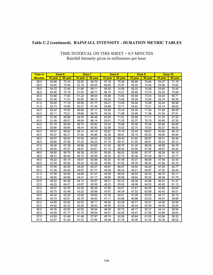
166

Table C.2 (continued). RAINFALL INTENSITY - DURATION METRIC TABLES

TIME INTERVAL ON THIS SHEET = 0.5 MINUTES Rainfall Intensity given in millimeters per hour.

10 year 50 year 10 year 50 year 10 year 50 year 10 year 50 year 10 year 50 year38.0 54.98 73.16 52.50 69.79 57.19 75.36 56.88 74.84 54.27 71.1938.5 54.65 72.83 52.18 69.45 56.85 74.97 56.55 74.46 53.96 70.8239.0 54.33 72.49 51.86 69.11 56.52 74.59 56.22 74.08 53.65 70.4539.5 54.00 72.16 51.54 68.77 56.19 74.21 55.90 73.70 53.35 70.0840.0 53.68 71.83 51.22 68.44 55.86 73.83 55.58 73.33 53.04 69.7140.5 53.36 71.51 50.90 68.10 55.53 73.46 55.26 72.95 52.74 69.3541.0 53.05 71.18 50.59 67.77 55.21 73.09 54.94 72.58 52.44 68.9841.5 52.73 70.85 50.27 67.44 54.88 72.71 54.62 72.21 52.14 68.6242.0 52.42 70.53 49.96 67.11 54.56 72.34 54.30 71.84 51.84 68.2642.5 52.11 70.21 49.66 66.79 54.24 71.98 53.99 71.48 51.54 67.9143.0 51.80 69.89 49.35 66.46 53.93 71.61 53.68 71.11 51.25 67.5543.5 51.49 69.57 49.04 66.14 53.61 71.25 53.37 70.75 50.95 67.2044.0 51.18 69.25 48.74 65.82 53.30 70.88 53.06 70.39 50.66 66.8544.5 50.88 68.94 48.44 65.50 52.98 70.52 52.75 70.03 50.37 66.5045.0 50.57 68.62 48.14 65.18 52.67 70.16 52.45 69.67 50.08 66.1545.5 50.27 68.31 47.84 64.86 52.36 69.81 52.15 69.32 49.80 65.8046.0 49.97 68.00 47.55 64.54 52.06 69.45 51.84 68.97 49.51 65.4646.5 49.68 67.69 47.25 64.23 51.75 69.10 51.55 68.61 49.23 65.1247.0 49.38 67.38 46.96 63.92 51.45 68.75 51.25 68.26 48.95 64.7847.5 49.09 67.07 46.67 63.61 51.15 68.40 50.95 67.92 48.67 64.4448.0 48.80 66.76 46.38 63.30 50.85 68.05 50.66 67.57 48.39 64.1048.5 48.51 66.46 46.10 62.99 50.55 67.70 50.36 67.23 48.11 63.7749.0 48.22 66.15 45.81 62.68 50.25 67.36 50.07 66.88 47.84 63.4349.5 47.93 65.85 45.53 62.38 49.96 67.02 49.78 66.54 47.56 63.1050.0 47.65 65.55 45.25 62.07 49.67 66.67 49.50 66.20 47.29 62.7750.5 47.36 65.25 44.97 61.77 49.38 66.34 49.21 65.87 47.02 62.4451.0 47.08 64.95 44.69 61.47 49.09 66.00 48.93 65.53 46.75 62.1151.5 46.80 64.66 44.41 61.17 48.80 65.66 48.64 65.20 46.48 61.7952.0 46.52 64.36 44.14 60.87 48.51 65.33 48.36 64.86 46.22 61.4752.5 46.25 64.07 43.87 60.58 48.23 65.00 48.08 64.53 45.95 61.1553.0 45.97 63.78 43.59 60.28 47.95 64.67 47.81 64.20 45.69 60.8353.5 45.70 63.49 43.32 59.99 47.67 64.34 47.53 63.88 45.43 60.5154.0 45.42 63.20 43.06 59.69 47.39 64.01 47.26 63.55 45.17 60.1954.5 45.15 62.91 42.79 59.40 47.11 63.68 46.98 63.23 44.91 59.8855.0 44.89 62.62 42.53 59.11 46.83 63.36 46.71 62.91 44.65 59.5655.5 44.62 62.33 42.26 58.83 46.56 63.04 46.44 62.59 44.40 59.2556.0 44.35 62.05 42.00 58.54 46.29 62.72 46.17 62.27 44.14 58.9456.5 44.09 61.77 41.74 58.26 46.01 62.40 45.91 61.95 43.89 58.6357.0 43.83 61.48 41.49 57.97 45.74 62.08 45.64 61.63 43.64 58.3357.5 43.57 61.20 41.23 57.69 45.48 61.76 45.38 61.32 43.39 58.02

Time in Minutes

Zone 9 Zone 10Zone 8Zone 6 Zone 7

167

Table C.2 (continued). RAINFALL INTENSITY - DURATION METRIC TABLES

TIME INTERVAL ON THIS SHEET = 1.0 MINUTES Rainfall Intensity given in millimeters per hour.

10 year 50 year 10 year 50 year 10 year 50 year 10 year 50 year 10 year 50 year58.0 43.31 60.92 40.97 57.41 45.21 61.45 45.12 61.01 43.14 57.7259.0 42.79 60.37 40.47 56.85 44.68 60.83 44.60 60.39 42.65 57.1260.0 42.29 59.82 39.97 56.30 44.16 60.21 44.08 59.77 42.16 56.5261.0 41.92 59.30 39.64 55.83 43.78 59.71 43.70 59.27 41.79 56.0562.0 41.57 58.79 39.30 55.37 43.41 59.21 43.32 58.78 41.43 55.5863.0 41.21 58.29 38.98 54.92 43.04 58.72 42.94 58.28 41.06 55.1264.0 40.86 57.79 38.65 54.46 42.68 58.23 42.57 57.80 40.70 54.6665.0 40.51 57.29 38.33 54.01 42.31 57.74 42.19 57.31 40.35 54.2066.0 40.16 56.80 38.01 53.57 41.95 57.26 41.83 56.83 39.99 53.7567.0 39.82 56.31 37.69 53.13 41.60 56.79 41.46 56.36 39.64 53.3068.0 39.48 55.83 37.37 52.69 41.24 56.31 41.10 55.88 39.29 52.8669.0 39.14 55.35 37.06 52.25 40.89 55.84 40.74 55.42 38.95 52.4270.0 38.80 54.87 36.75 51.82 40.54 55.38 40.39 54.95 38.60 51.9871.0 38.47 54.40 36.44 51.39 40.20 54.92 40.04 54.49 38.27 51.5572.0 38.14 53.93 36.14 50.97 39.86 54.46 39.69 54.03 37.93 51.1273.0 37.81 53.47 35.84 50.55 39.52 54.01 39.34 53.58 37.60 50.6974.0 37.49 53.01 35.54 50.13 39.18 53.56 39.00 53.13 37.27 50.2775.0 37.17 52.55 35.24 49.72 38.85 53.11 38.66 52.69 36.94 49.8576.0 36.85 52.10 34.94 49.31 38.52 52.67 38.32 52.25 36.62 49.4477.0 36.54 51.65 34.65 48.90 38.19 52.23 37.99 51.81 36.29 49.0378.0 36.22 51.21 34.36 48.50 37.86 51.79 37.66 51.38 35.98 48.6279.0 35.91 50.77 34.07 48.10 37.54 51.36 37.33 50.95 35.66 48.2180.0 35.61 50.33 33.79 47.70 37.22 50.93 37.00 50.52 35.35 47.8181.0 35.30 49.90 33.51 47.31 36.91 50.51 36.68 50.10 35.04 47.4182.0 35.00 49.47 33.23 46.91 36.59 50.09 36.36 49.68 34.73 47.0283.0 34.70 49.04 32.95 46.53 36.28 49.67 36.04 49.26 34.42 46.6384.0 34.40 48.62 32.67 46.14 35.97 49.26 35.73 48.85 34.12 46.2485.0 34.11 48.20 32.40 45.76 35.67 48.85 35.42 48.44 33.82 45.8586.0 33.81 47.79 32.13 45.38 35.36 48.44 35.11 48.03 33.52 45.4787.0 33.53 47.38 31.86 45.01 35.06 48.04 34.80 47.63 33.23 45.0988.0 33.24 46.97 31.59 44.64 34.76 47.64 34.50 47.23 32.94 44.7289.0 32.95 46.57 31.33 44.27 34.47 47.24 34.20 46.84 32.65 44.3490.0 32.67 46.17 31.07 43.91 34.17 46.85 33.90 46.44 32.36 43.9791.0 32.39 45.77 30.81 43.54 33.88 46.46 33.61 46.05 32.08 43.6192.0 32.11 45.38 30.55 43.18 33.59 46.07 33.31 45.67 31.80 43.2493.0 31.84 44.99 30.29 42.83 33.31 45.69 33.02 45.29 31.52 42.8894.0 31.57 44.60 30.04 42.47 33.03 45.31 32.74 44.91 31.24 42.5395.0 31.30 44.22 29.79 42.12 32.74 44.93 32.45 44.53 30.97 42.1796.0 31.03 43.84 29.54 41.78 32.47 44.55 32.17 44.16 30.69 41.8297.0 30.76 43.46 29.29 41.43 32.19 44.18 31.89 43.79 30.43 41.4798.0 30.50 43.08 29.05 41.09 31.92 43.81 31.61 43.42 30.16 41.13

Time in Minutes

Zone 9 Zone 10Zone 6 Zone 7 Zone 8

168

Table C.2 (continued). RAINFALL INTENSITY - DURATION METRIC TABLES

TIME INTERVAL ON THIS SHEET = 2.0 MINUTES Rainfall Intensity given in millimeters per hour.

10 year 50 year 10 year 50 year 10 year 50 year 10 year 50 year 10 year 50 year100.0 29.98 42.35 28.56 40.41 31.37 43.09 31.06 42.70 29.63 40.44102.0 29.47 41.62 28.09 39.75 30.84 42.37 30.52 41.99 29.11 39.77104.0 28.97 40.91 27.62 39.10 30.32 41.67 29.99 41.28 28.60 39.11106.0 28.47 40.21 27.16 38.45 29.81 40.98 29.47 40.60 28.10 38.46108.0 27.99 39.52 26.71 37.82 29.30 40.30 28.96 39.92 27.61 37.83110.0 27.51 38.84 26.26 37.20 28.81 39.63 28.46 39.25 27.13 37.20112.0 27.04 38.18 25.82 36.59 28.32 38.97 27.96 38.60 26.66 36.58114.0 26.58 37.52 25.39 35.99 27.84 38.33 27.48 37.95 26.19 35.97116.0 26.13 36.88 24.97 35.39 27.37 37.69 27.00 37.32 25.73 35.38118.0 25.68 36.25 24.55 34.81 26.90 37.06 26.53 36.70 25.28 34.79120.0 25.24 35.63 24.15 34.24 26.45 36.45 26.07 36.09 24.84 34.21122.0 24.98 35.16 23.89 33.79 26.17 36.00 25.80 35.63 24.58 33.79124.0 24.73 34.70 23.64 33.34 25.91 35.55 25.54 35.19 24.33 33.37126.0 24.47 34.24 23.39 32.90 25.64 35.11 25.27 34.75 24.08 32.95128.0 24.22 33.79 23.15 32.46 25.38 34.68 25.01 34.31 23.83 32.54130.0 23.97 33.35 22.91 32.03 25.12 34.25 24.76 33.88 23.59 32.14132.0 23.73 32.91 22.67 31.61 24.86 33.82 24.50 33.46 23.35 31.74134.0 23.48 32.47 22.43 31.19 24.60 33.40 24.25 33.04 23.10 31.35136.0 23.24 32.05 22.19 30.78 24.35 32.99 24.00 32.62 22.87 30.96138.0 23.00 31.62 21.96 30.37 24.10 32.58 23.75 32.22 22.63 30.57140.0 22.77 31.21 21.73 29.97 23.86 32.18 23.50 31.81 22.40 30.19142.0 22.53 30.80 21.50 29.57 23.61 31.78 23.26 31.41 22.17 29.82144.0 22.30 30.39 21.28 29.18 23.37 31.38 23.02 31.02 21.94 29.45146.0 22.07 29.99 21.05 28.79 23.13 31.00 22.78 30.63 21.72 29.08148.0 21.85 29.60 20.83 28.41 22.89 30.61 22.55 30.25 21.49 28.72150.0 21.62 29.21 20.61 28.03 22.66 30.23 22.32 29.87 21.27 28.37152.0 21.40 28.82 20.40 27.66 22.43 29.86 22.09 29.49 21.05 28.01154.0 21.18 28.44 20.18 27.29 22.20 29.49 21.86 29.12 20.84 27.67156.0 20.96 28.07 19.97 26.93 21.97 29.12 21.63 28.76 20.62 27.32158.0 20.75 27.70 19.76 26.58 21.74 28.76 21.41 28.40 20.41 26.98160.0 20.54 27.34 19.56 26.22 21.52 28.41 21.19 28.04 20.20 26.65162.0 20.33 26.98 19.35 25.88 21.30 28.05 20.97 27.69 19.99 26.32164.0 20.12 26.62 19.15 25.53 21.08 27.71 20.75 27.34 19.79 25.99166.0 19.91 26.27 18.95 25.20 20.86 27.36 20.54 27.00 19.58 25.67168.0 19.71 25.92 18.75 24.86 20.65 27.02 20.33 26.66 19.38 25.35

Time in Minutes

Zone 9 Zone 10Zone 8Zone 6 Zone 7

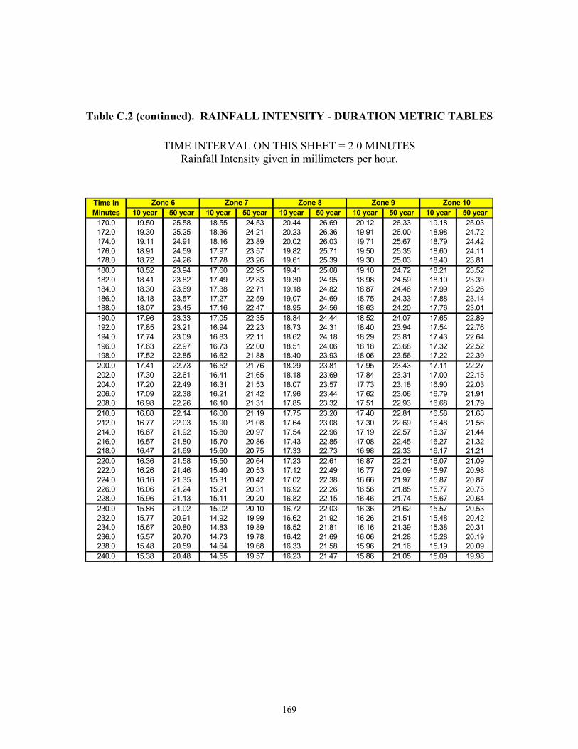
169

Table C.2 (continued). RAINFALL INTENSITY - DURATION METRIC TABLES

TIME INTERVAL ON THIS SHEET = 2.0 MINUTES Rainfall Intensity given in millimeters per hour.

10 year 50 year 10 year 50 year 10 year 50 year 10 year 50 year 10 year 50 year170.0 19.50 25.58 18.55 24.53 20.44 26.69 20.12 26.33 19.18 25.03172.0 19.30 25.25 18.36 24.21 20.23 26.36 19.91 26.00 18.98 24.72174.0 19.11 24.91 18.16 23.89 20.02 26.03 19.71 25.67 18.79 24.42176.0 18.91 24.59 17.97 23.57 19.82 25.71 19.50 25.35 18.60 24.11178.0 18.72 24.26 17.78 23.26 19.61 25.39 19.30 25.03 18.40 23.81180.0 18.52 23.94 17.60 22.95 19.41 25.08 19.10 24.72 18.21 23.52182.0 18.41 23.82 17.49 22.83 19.30 24.95 18.98 24.59 18.10 23.39184.0 18.30 23.69 17.38 22.71 19.18 24.82 18.87 24.46 17.99 23.26186.0 18.18 23.57 17.27 22.59 19.07 24.69 18.75 24.33 17.88 23.14188.0 18.07 23.45 17.16 22.47 18.95 24.56 18.63 24.20 17.76 23.01190.0 17.96 23.33 17.05 22.35 18.84 24.44 18.52 24.07 17.65 22.89192.0 17.85 23.21 16.94 22.23 18.73 24.31 18.40 23.94 17.54 22.76194.0 17.74 23.09 16.83 22.11 18.62 24.18 18.29 23.81 17.43 22.64196.0 17.63 22.97 16.73 22.00 18.51 24.06 18.18 23.68 17.32 22.52198.0 17.52 22.85 16.62 21.88 18.40 23.93 18.06 23.56 17.22 22.39200.0 17.41 22.73 16.52 21.76 18.29 23.81 17.95 23.43 17.11 22.27202.0 17.30 22.61 16.41 21.65 18.18 23.69 17.84 23.31 17.00 22.15204.0 17.20 22.49 16.31 21.53 18.07 23.57 17.73 23.18 16.90 22.03206.0 17.09 22.38 16.21 21.42 17.96 23.44 17.62 23.06 16.79 21.91208.0 16.98 22.26 16.10 21.31 17.85 23.32 17.51 22.93 16.68 21.79210.0 16.88 22.14 16.00 21.19 17.75 23.20 17.40 22.81 16.58 21.68212.0 16.77 22.03 15.90 21.08 17.64 23.08 17.30 22.69 16.48 21.56214.0 16.67 21.92 15.80 20.97 17.54 22.96 17.19 22.57 16.37 21.44216.0 16.57 21.80 15.70 20.86 17.43 22.85 17.08 22.45 16.27 21.32218.0 16.47 21.69 15.60 20.75 17.33 22.73 16.98 22.33 16.17 21.21220.0 16.36 21.58 15.50 20.64 17.23 22.61 16.87 22.21 16.07 21.09222.0 16.26 21.46 15.40 20.53 17.12 22.49 16.77 22.09 15.97 20.98224.0 16.16 21.35 15.31 20.42 17.02 22.38 16.66 21.97 15.87 20.87226.0 16.06 21.24 15.21 20.31 16.92 22.26 16.56 21.85 15.77 20.75228.0 15.96 21.13 15.11 20.20 16.82 22.15 16.46 21.74 15.67 20.64230.0 15.86 21.02 15.02 20.10 16.72 22.03 16.36 21.62 15.57 20.53232.0 15.77 20.91 14.92 19.99 16.62 21.92 16.26 21.51 15.48 20.42234.0 15.67 20.80 14.83 19.89 16.52 21.81 16.16 21.39 15.38 20.31236.0 15.57 20.70 14.73 19.78 16.42 21.69 16.06 21.28 15.28 20.19238.0 15.48 20.59 14.64 19.68 16.33 21.58 15.96 21.16 15.19 20.09240.0 15.38 20.48 14.55 19.57 16.23 21.47 15.86 21.05 15.09 19.98

Time in Minutes

Zone 9 Zone 10Zone 6 Zone 7 Zone 8

170

Appendix D Selected Isopluvial Maps

Figure D.1: Isopluvial Map of 2-Year, 10-Minute Rainfall Intensity

171

Figure D.2: Isopluvial Map of 2-Year, 1-Hour Rainfall Intensity

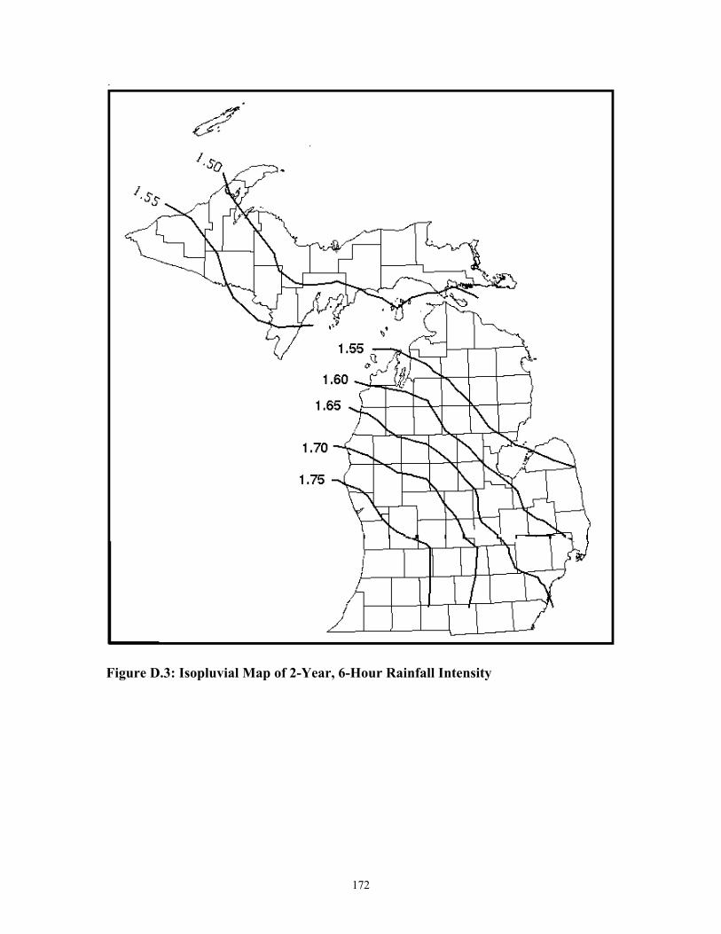
172

Figure D.3: Isopluvial Map of 2-Year, 6-Hour Rainfall Intensity

173

Figure D.4: Isopluvial Map of 2-Year, 24-Hour Rainfall Intensity

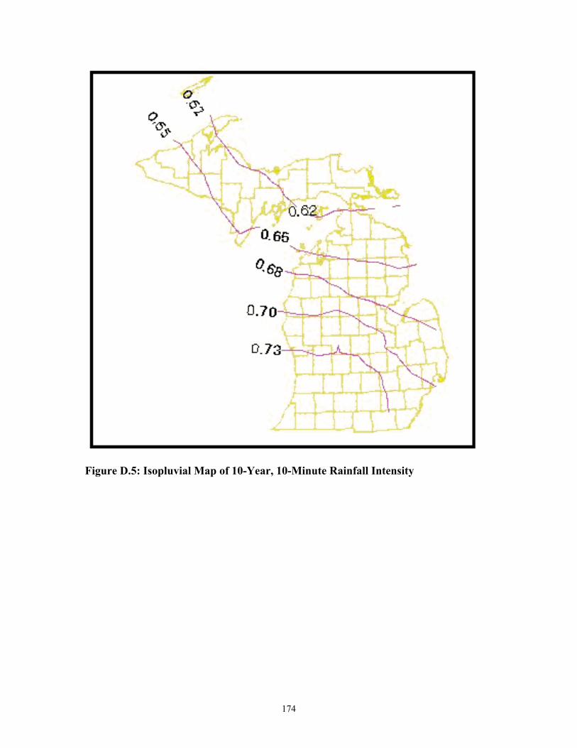
174

Figure D.5: Isopluvial Map of 10-Year, 10-Minute Rainfall Intensity

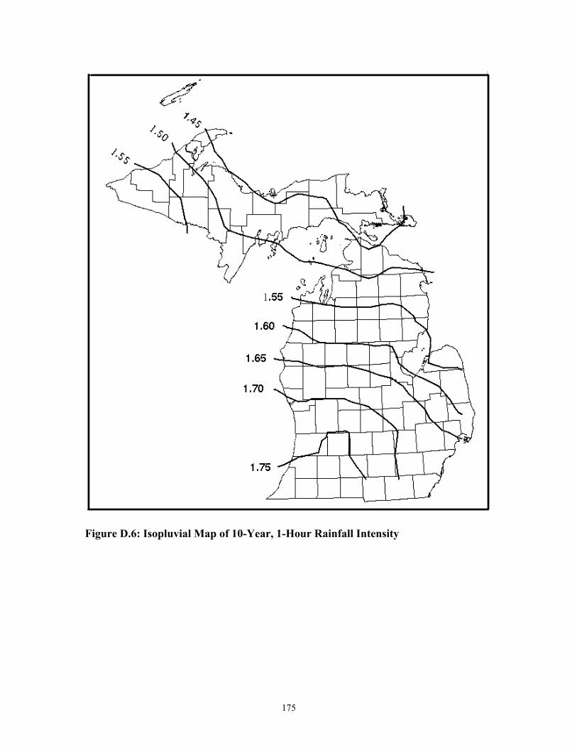
175

Figure D.6: Isopluvial Map of 10-Year, 1-Hour Rainfall Intensity

176

Figure D.7: Isopluvial Map of 10-Year, 6-Hour Rainfall Intensity

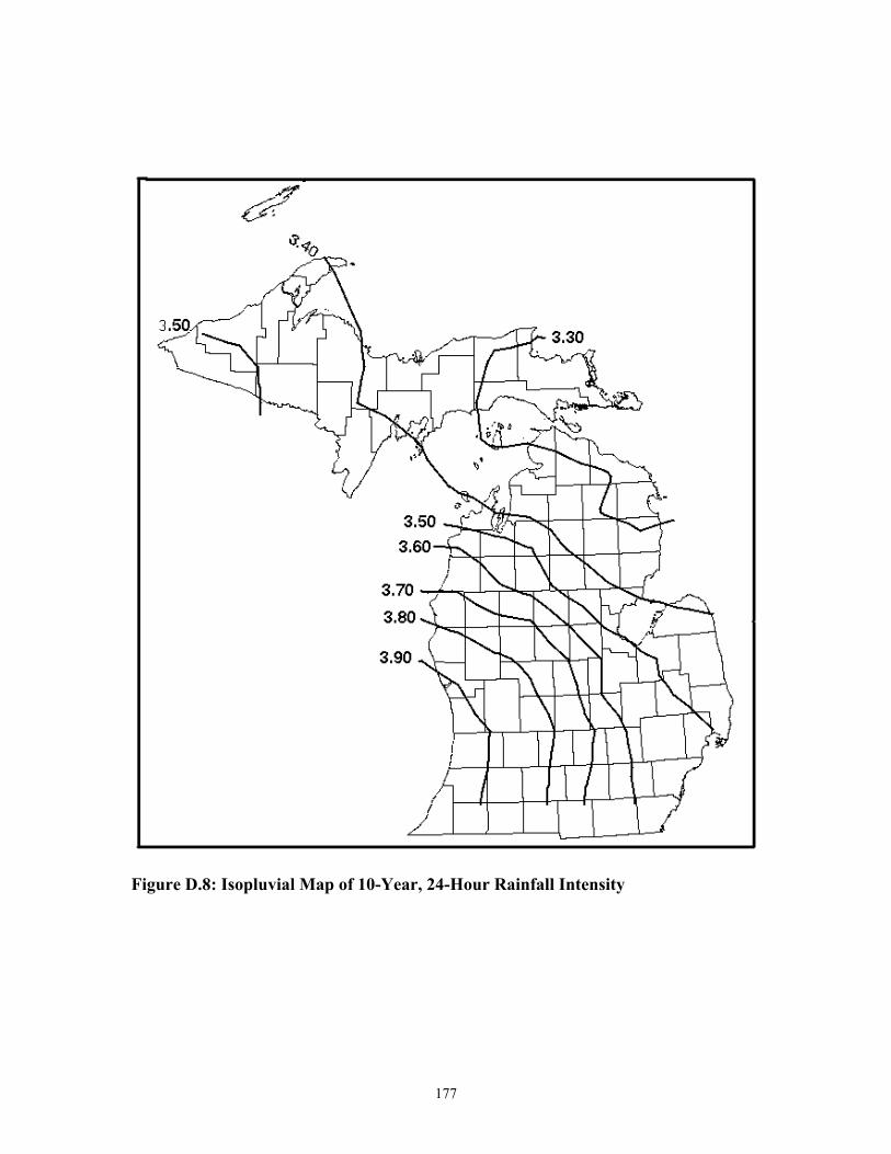
177

Figure D.8: Isopluvial Map of 10-Year, 24-Hour Rainfall Intensity

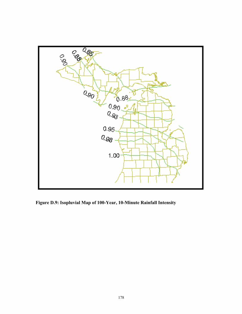
178

Figure D.9: Isopluvial Map of 100-Year, 10-Minute Rainfall Intensity

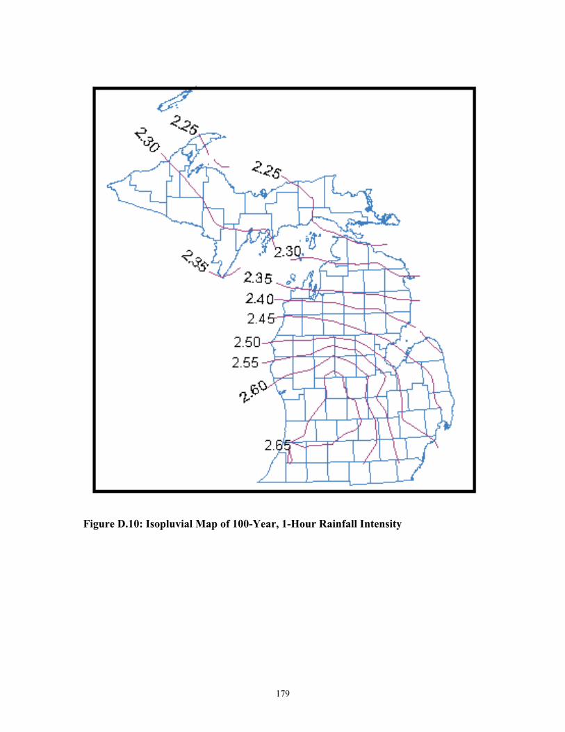
179

Figure D.10: Isopluvial Map of 100-Year, 1-Hour Rainfall Intensity

180

Figure D.11: Isopluvial Map of 100-Year, 6-Hour Rainfall Intensity

181

Figure D.12: Isopluvial Map of 100-Year, 24-Hour Rainfall Intensity

182

Appendix E Kriging Theory and Results

E.1 Mathematical Basis of Kriging

Kriging, like other linear estimation methods, models the spatial behavior of a

random variable, such as rainfall IDF estimates, by estimating unknown values from a

weighted average of observed values. However, unlike other methods, kriging

determines the weighted average based on the orientation (i.e., distance and direction) of

the observed point values with respect to the unknown value location. Thus, kriging

more appropriately describes/measures the similarity between an unknown location and

neighboring observations (Clark 1987). Based on several underlying assumptions, the

weights are assigned so that the sum of the weights equals to 1 (i.e., unbiased estimate).

Kriging is advantageous over other methods because: 1) its results are reproducible; 2) it

relies on an explicit model of spatial variability; 3) it provides “best” estimates and

measures of the reliability of the estimates; and 4) it is less labor-intensive and more

objective than other methods (Kitanidis 1993).

The process of geostatistical linear estimation involves two main steps: structural

analysis and best linear unbiased estimation (BLUE). In general, structural analysis is the

identification of a theoretical semivariogram model used to characterize the spatial

variability in the variable of interest. BLUE uses the semivariogram model parameters to

determine the interpolated estimates, which are unbiased and have a minimum variance.

In the initial assessment of the six spatial interpolation algorithms, only brief

descriptions of geostatistics, ordinary kriging, and the semivariogram were given. This

section will review, in more detail, ordinary kriging by focusing on underlying statistical

assumptions, the semivariogram, and on the assignment of weights used in the kriging

183

process. In addition, spatial averaging of point estimates through block kriging will be

discussed.

E.1.1 Underlying Statistical Assumptions of Ordinary Kriging

In general linear estimation, the spatial variable of interest represents a collection

of random values distributed over space or time as described by a random function. In

geostatistics, the random function is assumed to be characterized by three components: 1)

a structural component, having a constant mean or trend; 2) a random, but spatially

correlated component, i.e., regionalized variable; and 3) a spatially uncorrelated

component (random noise or residual error) (Burrough and McDonnell 1998). This

characterization of the random function is known as the regionalized variable theory,

which is the foundation of geostatistics (Armstrong 1998). Equation E.1 illustrates the

mathematical representation of the regionalized variable theory (Burrough and

McDonnell 1998).

εε ′′+′+= )()()( xxmxZ (E.1)

Letting x represent the position in 1, 2, or 3 dimensions, Z is a random variable at x,

( )m x is the structural component of Z at x, ( )xε ′ is the regionalized variable, and ( )xε ′′

is the spatially uncorrelated component. Figure E.1 illustrates the three components that

characterize the regionalized variable theory.

184

Figure E.1. Three components of the regionalized variable theory, where (i) is the structural component; (ii) is the random, but spatially correlated component; and (iii) is the spatially uncorrelated component (Burrough and McDonnell 1998).

The spatial variable is referred to as a regionalized variable and initially assumed

stationary (Hohn 1988). The concept of stationarity infers that all moments of the

variable are homogeneous and self-repeating in space or time (Armstrong 1998). Since

strict stationarity cannot typically be verified due to a lack of sampled data, only the

mean and covariance are typically required to be constant, a condition termed “second

order stationarity” (Armstrong 1998). If the regionalized variable is unable to satisfy

second order stationarity, a less restrictive condition is the intrinsic hypothesis, which

only restricts the first moment, i.e. mean, to be constant with respect to its position (Hohn

1988). Under the intrinsic hypothesis, the following assumptions can be made: 1) )(xm

equals the mean value of the sampling area; 2) the average or expected difference

between any two locations x and x + h, separated by a distance vector h, will be zero; and

3) the variance of difference depends only on the distance h between sites (Burrough and

185

McDonnell 1998). The two assumptions are known as the stationarity of difference and

variance of differences, respectively.

[ ] 0)()( =+− hxZxZE (E.2)

)(2])}()([{ 2 hhxZxZE γ=+− (E.3)

where )(hγ is known as the semivariance. The intrinsic hypothesis states that once

structural effects have been accounted for, the remaining variation is homogeneous, i.e.,

differences between sites are only a function of distance (Armstrong 1998). Equation E.4

illustrates the equivalence between ( )xε ′ and )(hγ by rewriting Equation E.1.

εγ ′′++= )()()( hxmxZ (E.4)

By definition of the intrinsic hypothesis, Equation E.5 is the mathematical definition of

the experimental semivariogram ( )(ˆ hγ ) and can be used to estimate the expected

difference in value between pairs of samples with a given relative orientation (Clark

1987).

∑=

+−=n

iii hxzxz

nh

1

2)}()({21)(γ̂ (E.5)

where n is the number of observations in the sample of the attribute z separated by

distance h, known as the lag distance.

Prior to calculating the semivariance of the sample data, an appropriate range of

lag distances must be identified (similar to bin size in a histogram). The range in lag

distances should be no greater than one half the width of the area being sampled and no

less than the smallest sampling distance to ensure that each lag distance contains at least

3 or 4 calculated semivariance values (Burrough and McDonnell 1998; Hohn 1988). A

lag distance approximately equal to the average sample spacing would be an acceptable

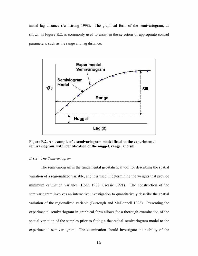
186

initial lag distance (Armstrong 1998). The graphical form of the semivariogram, as

shown in Figure E.2, is commonly used to assist in the selection of appropriate control

parameters, such as the range and lag distance.

Figure E.2. An example of a semivariogram model fitted to the experimental semivariogram, with identification of the nugget, range, and sill.

E.1.2 The Semivariogram

The semivariogram is the fundamental geostatistical tool for describing the spatial

variation of a regionalized variable, and it is used in determining the weights that provide

minimum estimation variance (Hohn 1988; Cressie 1991). The construction of the

semivariogram involves an interactive investigation to quantitatively describe the spatial

variation of the regionalized variable (Burrough and McDonnell 1998). Presenting the

experimental semivariogram in graphical form allows for a thorough examination of the

spatial variation of the samples prior to fitting a theoretical semivariogram model to the

experimental semivariogram. The examination should investigate the stability of the

187

semivariogram and presence of anisotropic effects that may be characteristic of the

regionalized variable.

The stability of experimental semivariogram can be investigated through an

iterative process of recalculating the experimental semivariogram at several lag distances

within the previously identified range. The experimental semivariogram may be

considered stable or well behaved if the position of the semivariogram between the origin

and the sill remains relatively stationary (i.e., there is little fluctuation in the vertical

direction) while the lag distance changes. For matters of convenience, the stability of the

semivariogram should be investigated assuming isotropic conditions, whereby the

covariance function depends only on the separation distance and all directional effects are

ignored (Kitanidis 1993). In this case, the calculated semivariogram is actually the

average semivariogram over all directions (Burrough and McDonnell 1998). Figure E.3

illustrates the shape of the neighborhood search radius assuming isotropic conditions.

Figure E.3. Illustration of the neighborhood search radius assuming isotropic conditions.

188

However, the assumption of isotropic conditions is not realistic for many natural systems,

so consideration of directional effects is recommended to model the spatial variation in

the data.

If the semivariogram can be determined as stable, the presence of anisotropic

conditions may be investigated to correct for any directional effects that may be present.

Two directional categories of anisotropies exist, geometric and zonal anisotropy, that are

defined by principal search direction, half-angles, and bandwidths. Figure E.4 illustrates

the search method used in calculating the semivariance of an unsampled location (P1)

while considering geometric anisotropies. Neighboring sample points are divided up by

the lag cutoffs determined by the chosen lag distance. It should also be noticed that by

selecting inappropriate half-angles and bandwidths, some sample points (e.g., P3) may

not be included in calculating the semivariogram. To avoid such situations, an

appropriate number of search directions or large enough half-angles should be used to

incorporate all sample points into the semivariogram. Zonal anisotropic effects are

similar but are manifested in a third dimension.

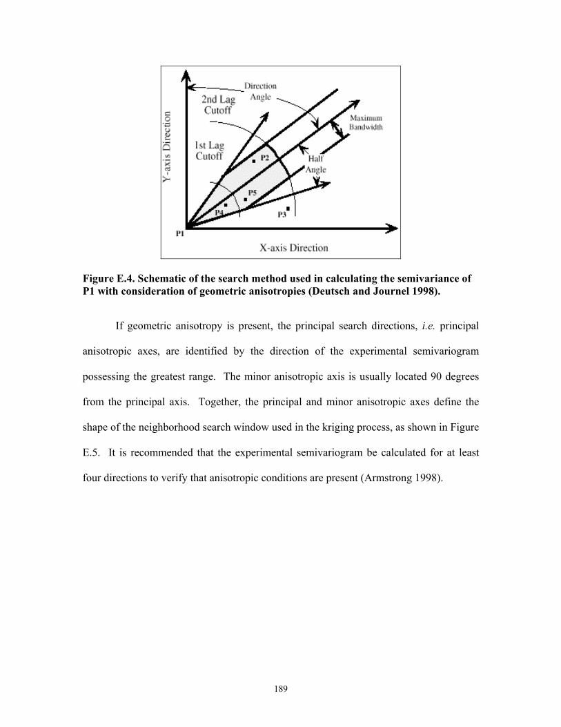
189

Figure E.4. Schematic of the search method used in calculating the semivariance of P1 with consideration of geometric anisotropies (Deutsch and Journel 1998).

If geometric anisotropy is present, the principal search directions, i.e. principal

anisotropic axes, are identified by the direction of the experimental semivariogram

possessing the greatest range. The minor anisotropic axis is usually located 90 degrees

from the principal axis. Together, the principal and minor anisotropic axes define the

shape of the neighborhood search window used in the kriging process, as shown in Figure

E.5. It is recommended that the experimental semivariogram be calculated for at least

four directions to verify that anisotropic conditions are present (Armstrong 1998).

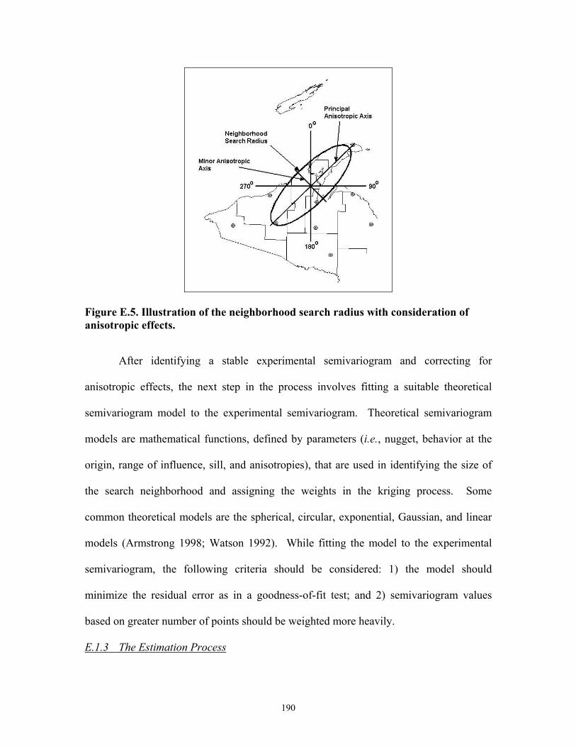
190

Figure E.5. Illustration of the neighborhood search radius with consideration of anisotropic effects.

After identifying a stable experimental semivariogram and correcting for

anisotropic effects, the next step in the process involves fitting a suitable theoretical

semivariogram model to the experimental semivariogram. Theoretical semivariogram

models are mathematical functions, defined by parameters (i.e., nugget, behavior at the

origin, range of influence, sill, and anisotropies), that are used in identifying the size of

the search neighborhood and assigning the weights in the kriging process. Some

common theoretical models are the spherical, circular, exponential, Gaussian, and linear

models (Armstrong 1998; Watson 1992). While fitting the model to the experimental

semivariogram, the following criteria should be considered: 1) the model should

minimize the residual error as in a goodness-of-fit test; and 2) semivariogram values

based on greater number of points should be weighted more heavily.

E.1.3 The Estimation Process

191

As previously discussed, the theoretical semivariogram model is used during the

kriging process to determine the appropriate interpolation weights. In ordinary kriging,

the structural component, i.e. mean )(xm , of the regionalized variable is assumed

unknown. An estimate at an unsampled point is given by (Burrough and McDonnell

1998):

∑=

⋅=n

iii xzxz

10 )()(ˆ λ (E.6)

where λi are the chosen weights, with ∑=

=n

ii

1

1λ so that the estimate is unbiased; )(ˆ 0xz is

the estimate; and )( ixz is a measurement at a sample point that is spatially correlated

with the estimate at point 0x . The variance of estimation is given by (Burrough and

McDonnell 1998):

φγλσ +⋅= ∑=

n

iiie xx

10

2 ),(ˆ (E.7)

where φ is a Lagrange multiplier associated with the unbiased constraint and ),( 0xxiγ is

the semivariance of z between points ix and the unsampled point 0x . For a detailed

derivation of the ordinary kriging system, the reader is referred to the following

references: Armstrong (1998), Clark (1987), Cressie (1991), Deutsch and Journel (1998),

Journel and Huijbregts (1978), and Kitanidis (1993).

E.1.4 Spatial Averaging Through Block Kriging

Equation E.6 and Equation E.7 represent point kriging, which implies that all

interpolated values relate to the area or volume of a sample, i.e. the support. For rainfall

IDF estimates, the support is typically only a few inches in diameter (the area of a rain

gage opening). Due to the high degree of short-range variation associated with these IDF

192

point estimates, ordinary point kriging may result in an interpolated surface possessing

sharp spikes and pits (Burrough and McDonnell 1998). In terms of modeling the spatial

behavior of IDF estimates, the presence of sharp spikes and pits within the interpolated

surface is not reasonable.

Short-range variation between the interpolated point estimates may be smoothed

using a method known as block kriging (Armstrong 1998). Block kriging provides a

means of estimating an average value of the regionalized variable over a specified area.

In an ordinary block kriging system, an average estimate )(ˆ Bxz at an unsampled block is

given by (Burrough and McDonnell 1998):

∑=

⋅=n

iiiB xzxz

1

)()(ˆ λ (E.8)

with ∑=

=n

ii

1

1λ , as before. However, the minimum variance is now (Burrough and

McDonnell 1998):

),(),(ˆ1

2 BBBxn

iii γφγλσ −+⋅= ∑

= (E.9)

where ),( Bxiγ is the average semivariance between point ix and the area B, as given by

Equation E.10 (Burrough and McDonnell 1998) and illustrated in Figure E.6.

∫ −⋅=B ii dxxx

BBx )(1),( γγ (E.10)

193

Figure E.6. Illustration of the process of averaging the semivariance between point xi and all sampled points within area B (Armstrong 1998).

Similarly, ( , )B Bγ is the average semivariance between any two points x and 'x

located within area B, as given by Equation A.12 (Burrough and McDonnell 1998) and

shown in Figure E.7.

')'(1),( 2 dxdxxxB

BB ∫∫ −⋅= γγ (E.12)

Figure E.7. Illustration of the process of averaging the semivariance between any two points x and x’ located within area B (Armstrong 1998).

xi

x x

x

B

x

x’

B

194

The estimation variance obtained using block kriging is inversely proportional to

the block area (B) (Armstrong 1998; Burrough and McDonnell 1998). For a detailed

derivation of the ordinary block kriging system, the reader is referred to Armstrong

(1998), Clark (1987), Cressie (1991), Deutsch and Journel (1998), Journel and Huijbregts

(1978), and Kitanidis (1993).

E.2 Results and Discussion

Preliminary rainfall IDF estimates in the form of isopluvial maps are presented

and discussed. The isopluvial maps are generated by applying trend surface analysis,

ordinary kriging, and universal kriging techniques to the spatial interpolation of a site-

specific distribution parameter (the mean of the AMS data). In addition, comparisons

between the preliminary rainfall IDF estimates and estimates presented by Huff and

Angel (1992) and Sorrell and Hamilton (1990) are provided. For brevity, only isopluvial

maps corresponding to the 2- and 100-year recurrence intervals and 1- and 24-hour

durations are presented for comparison of results.

E.2.1 Trend Surface Analysis Results

As discussed in Section 6.3.1, trend surface analysis uses multiple regression to fit

a polynomial surface to the entire set of sample observations, thereby generating an

interpolated surface that models the broad regional trend in the data. The trend surface

analysis results presented here were generated using UNCERT Version 1.20, a

geostatistical uncertainty analysis package (Wingle 1995). Figure E.8 illustrates

isopluvial maps of a) 2-year, 1- hour and b) 2-year, 24-hour rainfall intensities generated

by fitting a third-order trend surface to the AMS data. Figure E.9 illustrates isopluvial

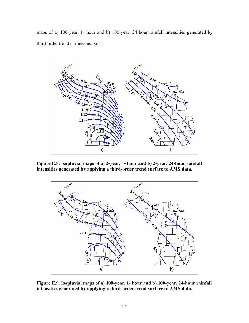
195

maps of a) 100-year, 1- hour and b) 100-year, 24-hour rainfall intensities generated by

third-order trend surface analysis.

Figure E.8. Isopluvial maps of a) 2-year, 1- hour and b) 2-year, 24-hour rainfall intensities generated by applying a third-order trend surface to AMS data.

Figure E.9. Isopluvial maps of a) 100-year, 1- hour and b) 100-year, 24-hour rainfall intensities generated by applying a third-order trend surface to AMS data.

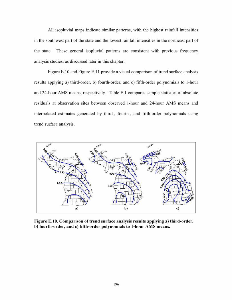
196

All isopluvial maps indicate similar patterns, with the highest rainfall intensities

in the southwest part of the state and the lowest rainfall intensities in the northeast part of

the state. These general isopluvial patterns are consistent with previous frequency

analysis studies, as discussed later in this chapter.

Figure E.10 and Figure E.11 provide a visual comparison of trend surface analysis

results applying a) third-order, b) fourth-order, and c) fifth-order polynomials to 1-hour

and 24-hour AMS means, respectively. Table E.1 compares sample statistics of absolute

residuals at observation sites between observed 1-hour and 24-hour AMS means and

interpolated estimates generated by third-, fourth-, and fifth-order polynomials using

trend surface analysis.

Figure E.10. Comparison of trend surface analysis results applying a) third-order, b) fourth-order, and c) fifth-order polynomials to 1-hour AMS means.

a) b) c)

197

Figure E.11. Comparison of trend surface analysis results applying a) third-order, b) fourth-order, and c) fifth-order polynomials to 24-hour AMS means.

Table E.1. Sample statistics of absolute residuals at observation sites. Residuals are the differences between observed 1-hour and 24-hour AMS means and interpolated

estimates generated by third-, fourth-, and fifth-order polynomials using trend surface analysis.

Trend Surface Analysis

Duration

Sample

Statistics 3rd Order 4th Order 5th Order

Maximum 0.221 0.221 0.208

Minimum 0.002 0.000 0.003

Mean 0.061 0.060 0.055

1-hour

Standard Deviation 0.050 0.050 0.048

Maximum 0.282 0.258 0.249

Minimum 0.000 0.000 0.000

Mean 0.076 0.071 0.069

24-hour

Standard Deviation 0.063 0.056 0.054

a) b) c)

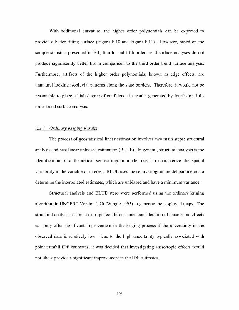
198

With additional curvature, the higher order polynomials can be expected to

provide a better fitting surface (Figure E.10 and Figure E.11). However, based on the

sample statistics presented in E.1, fourth- and fifth-order trend surface analyses do not

produce significantly better fits in comparison to the third-order trend surface analysis.

Furthermore, artifacts of the higher order polynomials, known as edge effects, are

unnatural looking isopluvial patterns along the state borders. Therefore, it would not be

reasonable to place a high degree of confidence in results generated by fourth- or fifth-

order trend surface analysis.

E.2.1 Ordinary Kriging Results

The process of geostatistical linear estimation involves two main steps: structural

analysis and best linear unbiased estimation (BLUE). In general, structural analysis is the

identification of a theoretical semivariogram model used to characterize the spatial

variability in the variable of interest. BLUE uses the semivariogram model parameters to

determine the interpolated estimates, which are unbiased and have a minimum variance.

Structural analysis and BLUE steps were performed using the ordinary kriging

algorithm in UNCERT Version 1.20 (Wingle 1995) to generate the isopluvial maps. The

structural analysis assumed isotropic conditions since consideration of anisotropic effects

can only offer significant improvement in the kriging process if the uncertainty in the

observed data is relatively low. Due to the high uncertainty typically associated with

point rainfall IDF estimates, it was decided that investigating anisotropic effects would

not likely provide a significant improvement in the IDF estimates.

199

In the structural analysis, the following criteria were considered in the selection

and fitting of semivariogram models to the experimental semivariograms: 1) minimum

variance (i.e., goodness-of-fit) to experimental semivariogram and 2) number of sample

pairs representing individual experimental semivariogram points. Figure E.12 illustrates

the results of the structural analysis performed on 1-hour AMS means by fitting a

spherical semivariogram model to the experimental semivariogram. Similarly, Figure

E.13 illustrates the results of the structural analysis performed on 24-hour AMS means by

fitting a Gaussian semivariogram model to the experimental semivariogram. At a lag

distance greater than 2,000,000 feet (≈ 380 miles), as shown in Figure E.13, an abrupt

linear rise in the experimental semivariogram occurs. Although the three furthermost

experimental semivariogram points are based on only a few pairs of observations, the

structural feature is indicative of a trend in the data. Appropriate treatment of the trend

will be further investigated and discussed in the following section on universal kriging.

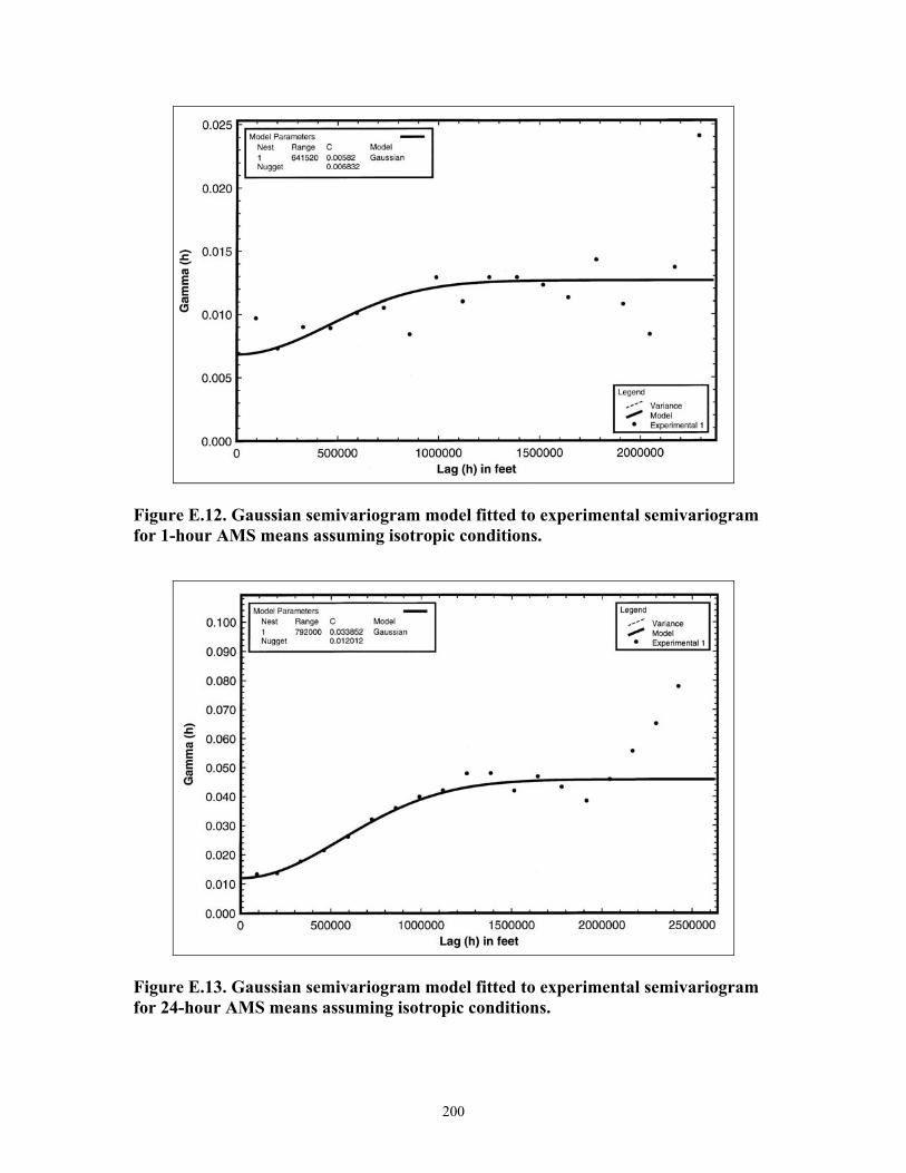
200

Figure E.12. Gaussian semivariogram model fitted to experimental semivariogram for 1-hour AMS means assuming isotropic conditions.

Figure E.13. Gaussian semivariogram model fitted to experimental semivariogram for 24-hour AMS means assuming isotropic conditions.

201

Model parameters defining the two Gaussian semivariogram models that were

fitted to the AMS 1-hour and 24-hour means, respectively, are given in Table E.2. A lag

distance of 132,000 feet (25 miles), equivalent to the average sample spacing, was

selected and used in the structural analysis of all the data used in this study.

Table E.2. Model parameters defining the semivariogram models that were fitted to the AMS 1-hour and 24-hour means.

Control Parameters 1-Hour Means 24-Hour Means

Lag Distance (feet) 132,000 132,000

Model Gaussian Gaussian

Nugget (in2) 0.0058 0.0120

Sill (in2) 0.0068 0.0339

Range of Influence (feet) 641,520 792,000

Ordinary kriging results are illustrated in Figure E.14 and Figure E.15. Figure

E.14 illustrates isopluvial maps of a) 2-year, 1- hour and b) 2-year, 24-hour rainfall

intensities, and Figure E.15 illustrates isopluvial maps of a) 100-year, 1- hour and b) 100-

year, 24-hour rainfall intensities. In both cases, results are based on AMS data.

202

Figure E.14. Isopluvial maps of a) 2-year, 1- hour and b) 2-year, 24-hour rainfall intensities generated by ordinary kriging on AMS data.

Figure E.15. Isopluvial maps of a) 100-year, 1- hour and b) 100-year, 24-hour rainfall intensities generated by ordinary kriging on AMS data.

a) b)

a) b)

203

E.2.3 Universal Kriging Results

In practice, universal kriging is used when a known trend exists in the data. The

process of universal kriging combines the theories of both trend surface analysis and

ordinary kriging. Trend surface analysis is first performed on the data to remove the

existing trend. Ordinary kriging is then performed on the residuals of the trend surface.

As a final step, the trend is added back into the ordinary kriging result performed on the

residuals.

Figure E.16 and Figure E.17 illustrate the experimental semivariograms of the

residuals from the 1-hour and 24-hour AMS means, respectively. For each experimental

semivariogram, no theoretical semivariogram model was suitable due to the phenomenon

known as a pure nugget effect. Identification of a pure nugget effect can be made when

the experimental semivariogram appears relatively flat (Journel and Huijbregts 1978).

Recall from Section 6.3.1, the nugget represents the discontinuity at the origin of the

semivariogram signifying the data is highly variable at distances shorter than the sample

spacing (Armstrong 1998). A pure nugget represents the absence of a spatial structure, or

spatial independence between the samples, thereby corresponding to “white noise” that

can not be corrected for at the current or larger sample spacing (Journel and Huijbregts

1978). Therefore, in this study, universal kriging appears to be incapable of improving

the IDF estimates provided by trend surface analysis or ordinary kriging.

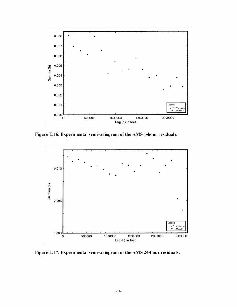
204

Figure E.16. Experimental semivariogram of the AMS 1-hour residuals.

Figure E.17. Experimental semivariogram of the AMS 24-hour residuals.

205

Appendix F Interactive GIS Model Though not fully tested and implemented, a prototype GIS model was developed

to query and display site-specific IDF curves based on the updated point IDF estimates

and regional frequency analysis results. This appendix outlines the tools used to develop

the interactive GIS model and instructions for using the model to obtain site-specific IDF

curves.

F.1 Tools Used in Development of Model

ArcView GIS Version 3.1, developed by Environmental Systems Research

Institute, Inc., was selected for this study due to package’s built in script language (i.e.,

Avenue) and customization functionality. In addition, ArcView GIS was chosen for its

common usage in the industry. The final product is a customized ArcView GIS project

file, called mdotidf.apr, which is compatible on both UNIX and PC platforms. The

project file contains four scripts written in Avenue script language. A brief description of

the functionality of the four scripts is presented in Table F.1 Proper execution of the

model is dependent on the existence of two GIS coverages, Counties and idf_grid. The

Counties coverage is a line coverage of Michigan’s county boundary lines and is used

only for visual orientation to select the site of interest. The idf_grid is the GIS grid

coverage with attribute table populated with the updated IDF estimates of six recurrence

intervals (0.5, 0.2, 0.1, 0.04, 0.02, 0.01 per year) and the seven durations (1, 2, 3, 6, 12,

18, and 24 hours).

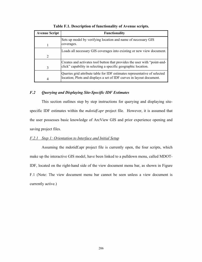
206

Table F.1. Description of functionality of Avenue scripts.

Avenue Script Functionality

1

Sets up model by verifying location and name of necessary GIS coverages.

2

Loads all necessary GIS coverages into existing or new view document.

3

Creates and activates tool button that provides the user with “point-and-click” capability in selecting a specific geographic location.

4

Queries grid attribute table for IDF estimates representative of selected location; Plots and displays a set of IDF curves in layout document.

F.2 Querying and Displaying Site-Specific IDF Estimates

This section outlines step by step instructions for querying and displaying site-

specific IDF estimates within the mdotidf.apr project file. However, it is assumed that

the user possesses basic knowledge of ArcView GIS and prior experience opening and

saving project files.

F.2.1 Step 1: Orientation to Interface and Initial Setup

Assuming the mdotidf.apr project file is currently open, the four scripts, which

make up the interactive GIS model, have been linked to a pulldown menu, called MDOT-

IDF, located on the right-hand side of the view document menu bar, as shown in Figure

F.1 (Note: The view document menu bar cannot be seen unless a view document is

currently active.)

207

Figure F.1 Location of MDOT-IDF menu pulldown.

The first step in querying and displaying site-specific IDF estimates is to ensure

that a view document, called “Select Location”, does not currently exist in the project’s

table of contents (TOC). If “Select Location” does not exist, open and make active a new

view document and continue to Step 2. If “Select Location” view does exist, open, make

active, and verify that the Counties and idf_grid coverages exist within the “Select

Location” view. If the two coverages have been loaded, leave “Select Location” active

and continue to Step 2.

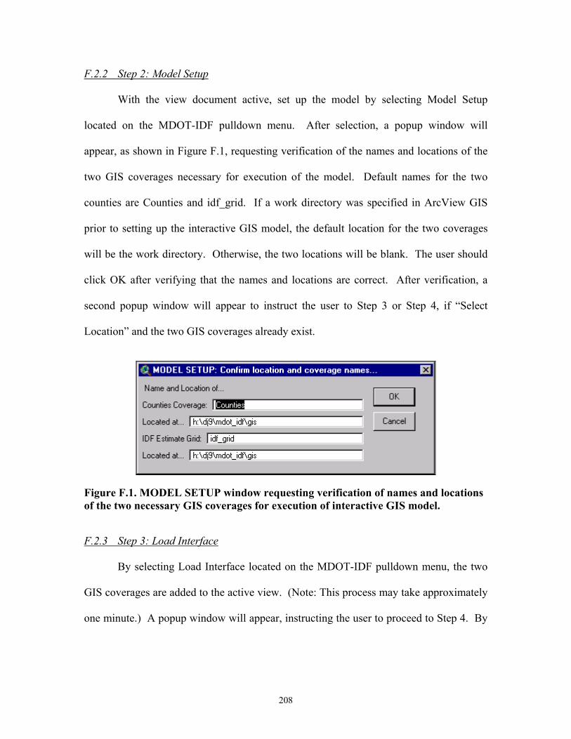
208

F.2.2 Step 2: Model Setup

With the view document active, set up the model by selecting Model Setup

located on the MDOT-IDF pulldown menu. After selection, a popup window will

appear, as shown in Figure F.1, requesting verification of the names and locations of the

two GIS coverages necessary for execution of the model. Default names for the two

counties are Counties and idf_grid. If a work directory was specified in ArcView GIS

prior to setting up the interactive GIS model, the default location for the two coverages

will be the work directory. Otherwise, the two locations will be blank. The user should

click OK after verifying that the names and locations are correct. After verification, a

second popup window will appear to instruct the user to Step 3 or Step 4, if “Select

Location” and the two GIS coverages already exist.

Figure F.1. MODEL SETUP window requesting verification of names and locations of the two necessary GIS coverages for execution of interactive GIS model.

F.2.3 Step 3: Load Interface

By selecting Load Interface located on the MDOT-IDF pulldown menu, the two

GIS coverages are added to the active view. (Note: This process may take approximately

one minute.) A popup window will appear, instructing the user to proceed to Step 4. By

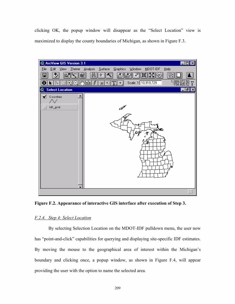
209

clicking OK, the popup window will disappear as the “Select Location” view is

maximized to display the county boundaries of Michigan, as shown in Figure F.3.

Figure F.2. Appearance of interactive GIS interface after execution of Step 3.

F.2.4. Step 4: Select Location

By selecting Selection Location on the MDOT-IDF pulldown menu, the user now

has “point-and-click” capabilities for querying and displaying site-specific IDF estimates.

By moving the mouse to the geographical area of interest within the Michigan’s

boundary and clicking once, a popup window, as shown in Figure F.4, will appear

providing the user with the option to name the selected area.

210

Figure F.3. Popup window providing option to input name of selected area.

The model will then query the attribute table of the grid coverage and plot the IDF

estimates in a layout document in the form of IDF curves, as shown in Figure F.5. (Note:

This process may take approximately one minute.)

Figure F.4. Plotted IDF curves for selected area generated by the interactive GIS model.

211

Appendix G Scale Invariance of Short Duration Data

G.1 Introduction

Since hourly precipitation data were much more widely available than short

duration (< 1 hour) data, a method was applied in which hourly precipitation data were

related to short duration data by assuming time scale invariance. This chapter explores

the validity of this assumption and recommends further research to develop reliable short-

duration IDF estimates.

In recent years, the study of phenomena with scale fluctuations has grown from

applications in physics phenomena such as statistical theories of turbulence and in

quantum field theory (Gupta and Waymire, 1990) to hydrologic phenomena such as

stochastic rain model application and intensity-duration-frequency (IDF) curve

formulation. While empirical equations have been used for nearly one hundred years to

explain the form of IDF curves, scale invariance has helped to understand these

relationships at a higher level. Sherman (1905) first developed a generalized IDF

relationship, and many other versions of this relationship have been developed in the

years since. All forms of the generalized IDF relationships assume that rainfall depth or

intensity is inversely related to the duration of a storm raised to a power, or scale factor.

A sampling of these studies will be reviewed.

Wenzel (1982) reported a generalized IDF relationship that expressed graphical

information from an IDF curve in mathematical form. This empirical equation was stated

as:

( )n

Ait b

=+ , (G.1)

212

where i is the intensity in inches per hour, A is a constant for a given return period, b and

n are constants independent of return period, and t is the duration in minutes. The

constants in this equation have been found to vary with location, and also should not be

applied beyond the range of intensity and duration for which they were developed.

Wenzel found that n varied from 0.40 to 0.84 around the nation for a ten-year return

period, with a value of 0.81 in Chicago. Wenzel concluded that n is very variable across

the nation depending on location.

Recently, this IDF relationship has been updated by Koutsoyiannis et al. (1998).

In this paper, a more consistent formulation of the IDF relationship was determined by

using a general formula for the relationship in which the specific forms are rigorously

derived from the underlying probability distribution function of the maximum intensities.

The general IDF relationship was determined to be

( )( )

a Tib d

= , (G.2)

where i is the intensity, T is the return period, and d is the duration of the storm. The

variable a(T) is determined from the probability distribution function of the maximum

intensity, and

( ) ( )b d d ηθ= + , (G.3)

where θ and η are parameters to be estimated (θ > 0, 0 < η < 1).

Applying this general relationship to data in Greece and noting the variation on

the parameters allowed Koutsoyiannis et al. to study the geographical variation of IDF

curves. The data were used from 13 recording stations uniformly distributed in a 25,000-

km2 area in Greece (1/5 the total area of Greece) where five major rivers are located. It

was determined that the η parameter could not be estimated accurately without the use of

213

short-duration (hourly) data. Also, the θ parameter could not be estimated accurately, but

it was determined that equating it to zero would be adequate. The geographical variation

of the η parameter was found to be very slight, and that more specifically, η can be

considered constant in each of the homogeneous subregions in this study area. The

parameters used to solve for a(T) do vary geographically. In conclusion, it was

determined that the proposed IDF relationship is an efficient parameterization and good

basis for the regionalization of the IDF relationship.

Although many previous studies depend on curve-fitting techniques, studies

applying scaling hypotheses to rainfall statistics have become popular over the past 20

years. These studies include Lovejoy and Schertzer (1985), Gupta and Waymire (1990),

Burlando and Rosso (1996), Menabde, Seed, and Pegram (1999), and Naghettini (2000).

Lovejoy and Schertzer (1985) showed that the atmosphere follows a symmetry

principle – termed generalized scale invariance - in which the statistical properties of the

small and large scale are related to each other by a magnification coupled with a

differential stratification from gravity and differential rotation from the Coriolis force.

This was shown through the use of two models, one that modeled the rainfall field using

a hierarchy of simple pulses, and a second that showed the scaling of the pulses. Lovejoy

and Schertzer concluded that this scale invariance principle and the models used to

illustrate it might become useful in future hydrologic studies, as they capture the extreme

variability of rain over a wide variety of scales in a very simple way.

Gupta and Waymire (1990) analyzed spatially averaged rainfall rates and river

flows to determine the nature of deviations from simple scaling. Simple scaling was

defined physically as a mathematical property in which probability distributions remain

214

invariant with respect to scaling by a function λθ, where λ > 0 is the spatial scale

parameter and θ is a characteristic exponent. In order to obtain empirical results,

continuous rainfall data was used from GATE (Global Atmosphere Research Program,

Atlantic Tropical Experiment). The first six statistical moments of the rainfall data were

calculated. These were the moments, hE Yλ , that corresponded to each λ value. In

order to examine the scaling properties, a conditional moment, mh, was expressed as:

log ( ) logh h hm aλ θ λ= + , (G.4)

where ah is the intercept, and θh is the slope. This conditional moment, mh(λ), was then

plotted versus λ on a log-log plot. The intercept (ah) and slope (θh) were found by

regression. From the graph, it was seen that there was a log-log linearity of the data. But

as h→hθ, the plot becomes nonlinear. Also θh was less than zero for all h analyzed. This

violates the assumption of linearity and of simple scaling in the wide and strict sense.

Therefore, simple scaling was not applicable, but the results of this paper show that if

multiscaling is used, hydrologic fluxes of continuous rainfall and river flow data can be

scaled down, similar to statistical theories of turbulence.

These results were taken one-step further by Burlando and Rosso (1996) as they

derived a method to create a general distribution-free framework to model extreme storm

probabilities from the scaling properties of observed rainfall data. A distribution-free

framework is then derived to model IDF curves based on either simple scaling or multi-

scaling assumptions. The simple scaling and multiscaling properties were applied to data

at two stations in Italy. In summary, Burlando and Rosso (1996) determined that both the

simple scaling and multiscaling log-normal models can be used to predict the growth

curve of rainfall depth in a design storm as a function of storm duration. Although some

215

of the observed data displayed simple scaling, multiscaling provides a more general

conceptual framework. Yet if a model follows simple scaling, the increase in model

performance will be small if multiscaling is used, and a lot more complex as multiscaling

involves many more parameters.

Building on the previous scaling work, Menabde et al. (1999) developed a simple

scaling methodology to use daily rainfall statistics to infer the IDF characteristics for

short-duration rainfall (less than one day). The scaling hypothesis was verified by fitting

the model to two different sets of data. The first data set was recorded in Melbourne,

Australia, representing the mid-Atlantic temperature climate with rainfall throughout the

year. The second data set was recorded in Warmbaths, South Africa representing a

warm, semi-arid climate with summer rainfall consisting mainly of convective storms. In

brief, this paper showed that the scaling hypothesis worked for two different rain gages in

two different climates. Menabde et al. (1999) also concluded that estimates of the scaling

coefficient (or scale factor), η, can be made using a shorter record of high-resolution rain

gages in the same climatic region. Once the scaling coefficient has been established for a

gage or set of gages in a region, short-duration IDF estimates can be obtained from the

analysis of daily data.

Similar to Menabde et al. (1999), Naghettini’s (2000) purpose was to derive an

IDF relationship for short duration rainfall from the statistical characteristics of daily data

using simple scaling relationships. Naghettini used the scaling hypothesis developed by

Menabde et al. (1999) to determine the scaling coefficient for the recording rainfall

gaging station of Vespasiano, located in Belo Horizonte, Brazil. It was determined that

the scaling coefficient for this station was equal to 0.69. IDF curves were deduced using

216

this coefficient and compared to curves derived from actual data. These curves matched

almost exactly. The scale factor, η, was also estimated for data observed at the Papagaios,

Lagoa do Gouvea, and Entre Rios de Minas stations located in the metropolitan region of

Belo Horizonte. Although there is a great distance between these stations, and they have

very different elevations and annual average rainfall depths, the simple scaling hypothesis

has been verified at these gages for durations greater than 45-minutes, with η varying

from 0.75 to 0.81. High values of the scaling factor show both that the short duration data

are more variable with respect to daily data and that the intensity of the short-duration

storms is relatively high.

G.2 Application of Scale Invariance Methodology to Data in Michigan

The assumption of scale-invariance was used to extrapolate short-duration IDF

results for Detroit to locations throughout the state. Specifically, given the estimate of n-

minute rainfall intensity for a given return period in the Detroit area, an estimate of n-

minute rainfall intensity for the same return period at another location was estimated as:

60

60n n xx D

D

II II

=

, (G.5)

where

-minute rainfall intensity at site nxI n x=

Average -minute rainfall intensity in the Detroit areanDI n=

60 60-minute rainfall intensity at site xI x=

60 Average 60-minute rainfall intensity in the Detroit areaDI =

217

The major assumption in this extrapolation method is that scaling relationships

are the same throughout the state, i.e., that there is one scaling factor that can be applied

to the entire state. In order to confirm this, the scale-invariance property was evaluated in

greater detail. Multiscaling is most often used in rainfall analysis, as it has been shown

that simple scaling does not work for continuous rainfall (Gupta and Waymire, 1990).

Recently, however, Menabde et al. (1999) have shown that simple scaling holds for

annual maximum series (AMS) of rainfall intensity. The verification method used by

Menabde et al. (1999) and Naghettini (2000) was used to verify the scaling assumption

applied in this study.

Simple scaling in the “strict sense” is defined as an equality of distributions by Menabde

et al. (1999):

dist

nnu u

η− = (G.6)

where

random variable with duration, nu n= ,

random variable with duration, u =¥ ¥ ,

scaling coefficientη = ,

scale ration η− =

,

and n> .

For the purposes of this study, this property was rewritten as:

60 6060

n nx D

x D

I InI I

η− = = (G.7)

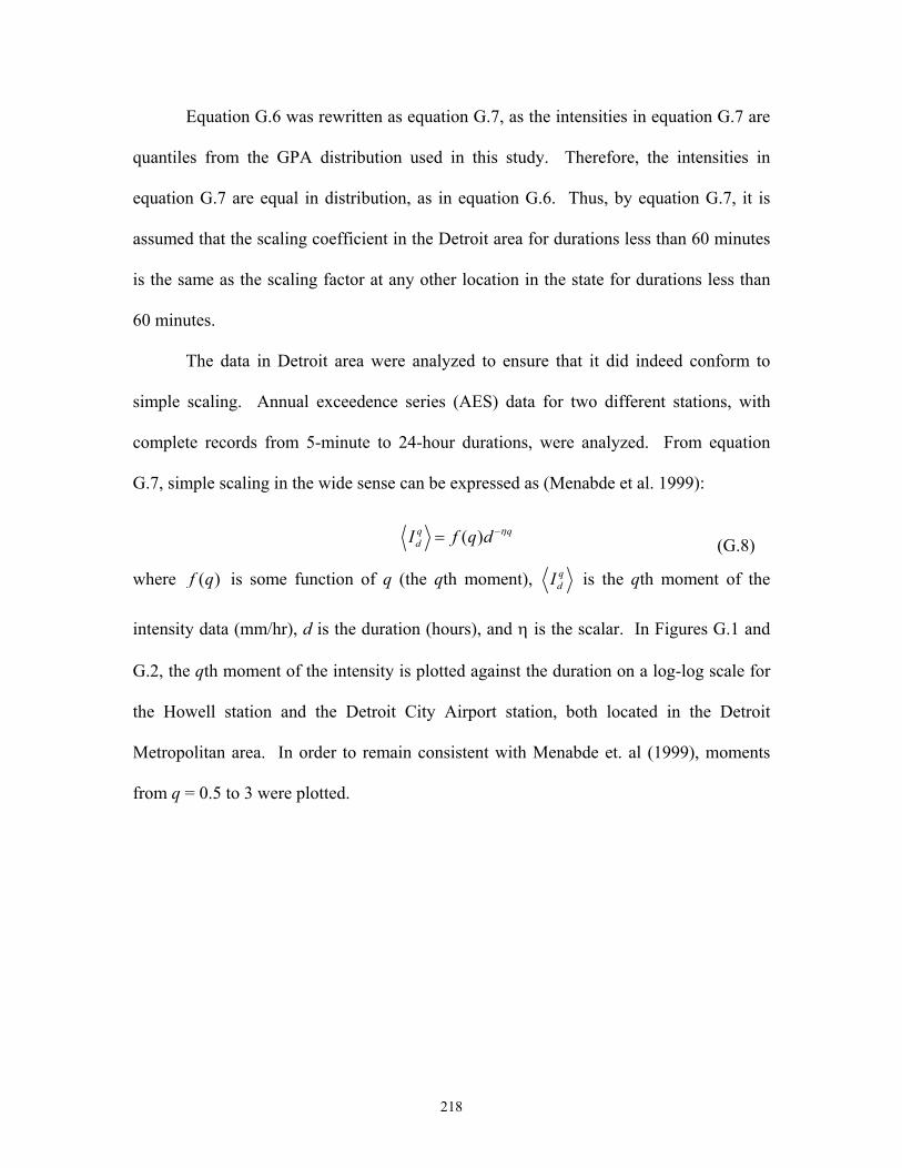
218

Equation G.6 was rewritten as equation G.7, as the intensities in equation G.7 are

quantiles from the GPA distribution used in this study. Therefore, the intensities in

equation G.7 are equal in distribution, as in equation G.6. Thus, by equation G.7, it is

assumed that the scaling coefficient in the Detroit area for durations less than 60 minutes

is the same as the scaling factor at any other location in the state for durations less than

60 minutes.

The data in Detroit area were analyzed to ensure that it did indeed conform to

simple scaling. Annual exceedence series (AES) data for two different stations, with

complete records from 5-minute to 24-hour durations, were analyzed. From equation

G.7, simple scaling in the wide sense can be expressed as (Menabde et al. 1999):

( )q qdI f q d η−= (G.8)

where ( )f q is some function of q (the qth moment), qdI is the qth moment of the

intensity data (mm/hr), d is the duration (hours), and η is the scalar. In Figures G.1 and

G.2, the qth moment of the intensity is plotted against the duration on a log-log scale for

the Howell station and the Detroit City Airport station, both located in the Detroit

Metropolitan area. In order to remain consistent with Menabde et. al (1999), moments

from q = 0.5 to 3 were plotted.

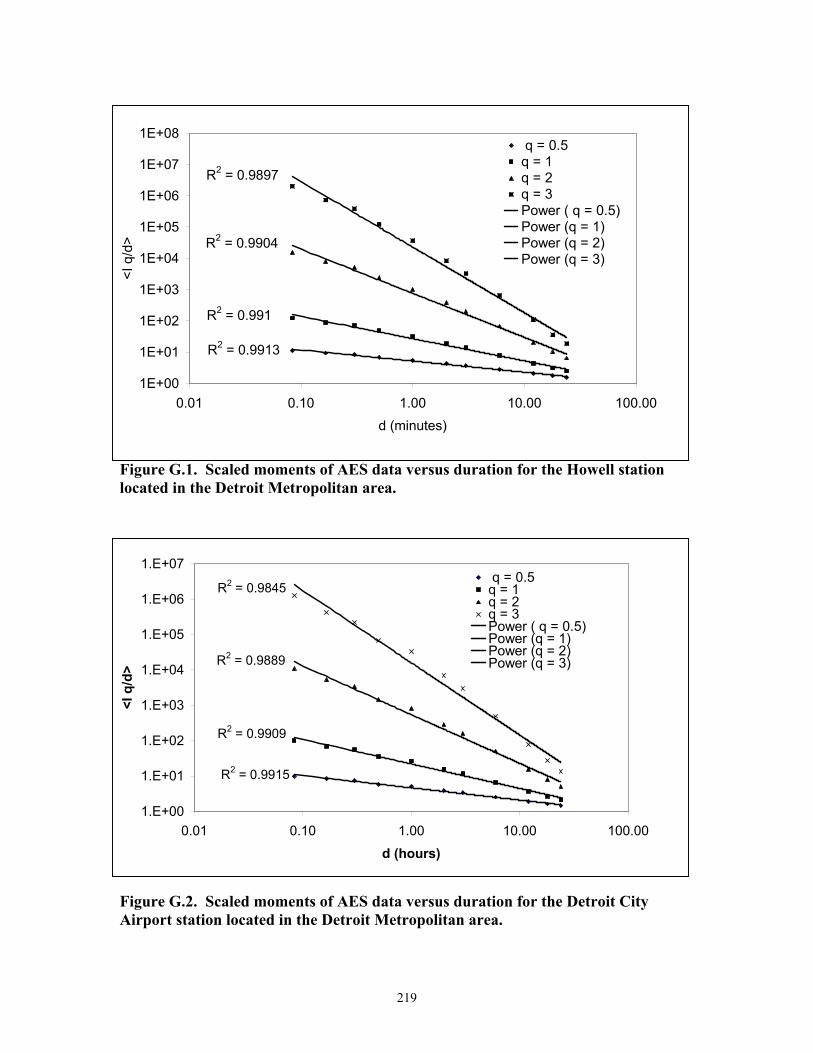
219

Figure G.1. Scaled moments of AES data versus duration for the Howell station located in the Detroit Metropolitan area.

Figure G.2. Scaled moments of AES data versus duration for the Detroit City Airport station located in the Detroit Metropolitan area.

R2 = 0.9913

R2 = 0.991

R2 = 0.9904

R2 = 0.9897

1E+00

1E+01

1E+02

1E+03

1E+04

1E+05

1E+06

1E+07

1E+08

0.01 0.10 1.00 10.00 100.00d (minutes)

<I q

/d>

q = 0.5q = 1q = 2q = 3Power ( q = 0.5)Power (q = 1)Power (q = 2)Power (q = 3)

R2 = 0.9915

R2 = 0.9909

R2 = 0.9889

R2 = 0.9845

1.E+00

1.E+01

1.E+02

1.E+03

1.E+04

1.E+05

1.E+06

1.E+07

0.01 0.10 1.00 10.00 100.00d (hours)

<I q

/d>

q = 0.5q = 1q = 2q = 3Power ( q = 0.5)Power (q = 1)Power (q = 2)Power (q = 3)

220

It can be seen from Figures G.1 and G.2 that the data are linearly related, and

there is not a break at duration of 60 minutes between the short- and long-duration data.

As both gages show a similar scaling relationship, it is possible that scaling may be

applicable in the Detroit area. From these plots, it was determined that there was a well-

defined scaling relationship for durations greater than or equal to ten minutes, but could

not be verified for less than ten minutes. In order to determine if the data follow simple

scaling or multi-scaling, the scaling exponent, -ηq, was plotted versus the moment, q, as

can be seen in Figure G.3. Once again the data were linearly related, with an R2 values of

0.9999 for the Howell station and 0.9993 for the Detroit City Airport station. Therefore,

simple scaling can be assumed in this situation. If the data had not been linear, then this

would have been a case of multi-scaling. The slope of this line is the scale factor, η,

which is 0.68 for the Howell station and 0.65 for the Detroit City Airport station. These

scale factors are quite close.

221

Figure G.3. The slope of the line provides an estimate of the scaling factor for the Howell station and the Detroit City Airport station in the Detroit Metropolitan area.

After verification of scaling of IDF estimates in the Detroit area, the assumption

of scaling was examined at a representative sample of stations throughout the state. The

only data readily available for less than the 1-hour duration for stations not in the Detroit

area are 15-minute continuous data from the National Oceanic and Atmospheric

Administration. An AMS data set was derived from the continuous data, and the first

four moments were calculated for durations of 15 minutes up to 24 hours. As with the

Detroit data, these moments were plotted against duration on a log-log scale to determine

whether scaling could be assumed.

Figures G.4 and G.5 show the scaling of the moments for the Gladwin station in

the central Lower Peninsula (L.P.) of Michigan and the Bruce Crossing station in the

northwest Upper Peninsula (U.P.) of Michigan, respectively. The linearity of the

moments seen here is similar to the other 22 stations that were examined, indicating that

y = 0.6761x + 0.0297R2 = 0.9999

y = 0.6535x + 0.0472R2 = 0.9993

0

0.5

1

1.5

2

2.5

3

3.5

4

0 1 2 3 4 5 6q

- ηq

HowellDetroit CityLinear (Howell)Linear (Detroit City)

222

for durations greater than 15 minutes, scaling appears to be applicable throughout

Michigan. As shown in Figure G.6, the scaling exponent, -ηq, was plotted versus the

moment, q, to determine if simple scaling is applicable and to estimate the scale factor for

stations throughout the state.

Figure G.4. Scaled moments of AMS data versus duration for the Gladwin station located in the central Lower Peninsula of Michigan.

R2 = 0.9985

R2 = 0.9992

R2 = 0.9991

R2 = 0.9987

1.E+00

1.E+01

1.E+02

1.E+03

1.E+04

1.E+05

1.E+06

1.E+07

0.1 1 10 100d (hours)

<I q

/d>

q = 0.5q = 1q = 2q = 3Power ( q = 0.5)Power (q = 1)Power (q = 2)Power (q = 3)

223

Figure G.5. Scaled moments of AMS data versus duration for the Bruce Crossing station located in the northwest Upper Peninsula of Michigan.

In Figure G.6, the scaling coefficients, or the slopes of the line, is 0.72 for the

Gladwin station, with a R2 value of 0.9999, and 0.73 for the Bruce Crossing station with a

R2 value of 1.0000 (The lines plot on top of one another). This indicates that simple

scaling could be applied at these two stations instead of the more complicated

multiscaling.

R2 = 0.9965

R2 = 0.9966

R2 = 0.9966

R2 = 0.9965

1.E+00

1.E+01

1.E+02

1.E+03

1.E+04

1.E+05

1.E+06

0.1 1 10 100d (hours)

<I q

/d>

q = 0.5q = 1q = 2q = 3Power ( q = 0.5)Power (q = 1)Power (q = 2)Power (q = 3)

224

Figure G.6. Linear relationship indicates simple scaling applicable at Bruce Crossing station in the northwest Upper Peninsula of Michigan and the Gladwin station in the central Lower Peninsula of Michigan.

The scaling coefficients of 0.72 and 0.73 found in Figure G.6 were typical for the

24 stations examined, with an average scalar equal to 0.72 and a standard deviation of

0.044. However, a few stations had significantly lower scalar exponents (as low as 0.62).

These stations were generally located on the western part of the Lower Peninsula, close

to or on Lake Michigan, as seen in Figure G.7, indicating that the effect of the lake

should be studied further. It can also be seen in Figure G.7 that the scaling coefficients

were generally higher in the northeastern part of the state.

y = 0.7288x + 0.0067R2 = 1.0000

y = 0.7233x + 0.0262R2 = 0.9999

0

0.5

1

1.5

2

2.5

3

3.5

4

0 1 2 3 4 5 6

q

- ηq

Bruce CrossingGladwinLinear (Bruce Crossing)Linear (Gladwin)

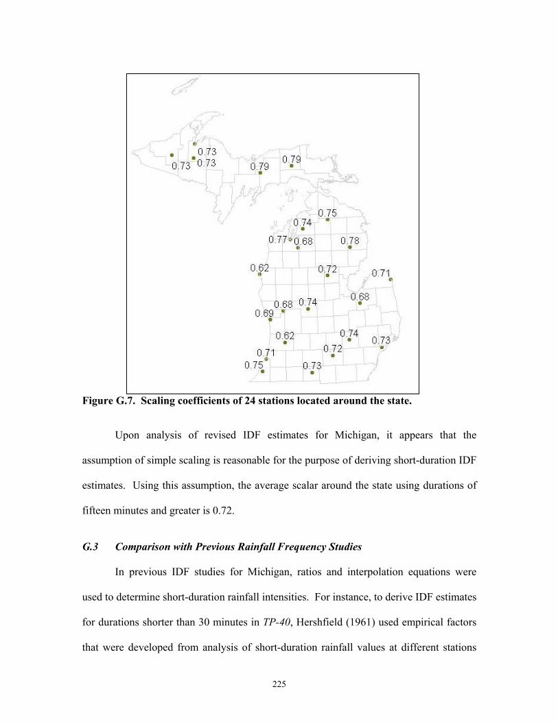
225

Figure G.7. Scaling coefficients of 24 stations located around the state.

Upon analysis of revised IDF estimates for Michigan, it appears that the

assumption of simple scaling is reasonable for the purpose of deriving short-duration IDF

estimates. Using this assumption, the average scalar around the state using durations of

fifteen minutes and greater is 0.72.

G.3 Comparison with Previous Rainfall Frequency Studies

In previous IDF studies for Michigan, ratios and interpolation equations were

used to determine short-duration rainfall intensities. For instance, to derive IDF estimates

for durations shorter than 30 minutes in TP-40, Hershfield (1961) used empirical factors

that were developed from analysis of short-duration rainfall values at different stations

226

around the country. These empirical ratios and the corresponding ratios developed for

comparison in this study are given in Table G.1. The ratios are very similar, with the new

ratios being the same as or slightly greater than the old. There may be several reasons for

these differences. First, Hershfield’s study included estimates for the entire United

States, and this study included estimates only for the State of Michigan. Also, nearly

forty years of additional data were used to calculate the new ratios. Sampling variability

in both studies may also have made a difference.

Table G.1. Comparison between the average relationship between 30-minute rainfall and rainfall for other durations for the same return period.

In NOAA Technical Memorandum NWS Hydro-35 (Hydro-35), Frederick et al.

(1977) found that the average ratios from TP-40 worked in many parts of the country, but

they have a geographic pattern and vary with return period. Although this study utilized

short duration data (data for durations from 5 to 60 minutes were obtained from recording

rain gages at approximately 200 NWS stations), an empirical equation was developed to

obtain isopluvial maps for the 10- and 30- minute durations:

2( ) (1 )( )n n m n mlR C R C R= + − (G.9)

Duration TP-40 New(min) Ratio Ratio

5 0.37 0.3910 0.57 0.5915 0.72 0.7260 1.27 1.43

227

where Rn is the required frequency value for N minutes, Rml and Rm2 are mapped values

for a lesser and longer duration, and Cn is the interpolation constant. The equations that

were adopted to obtain these values are as follows:

10-min value 0.59(15-min value) 0.41(5-min value)= + (G.10)

30-min value 0.49(60-min value) 0.51(15-min value)= + (G.11)

In order to interpolate short duration values for areas with only hourly recording stations,

the 2-year 60-minute map was created first and used as a guide to obtain shorter

durations.

In order to compare the new IDF estimates to those from Hydro-35, equations

G.10 and G.11 were applied to the new IDF estimates. For the 10-minute estimates, the

difference between the interpolation and scaling methods ranged from 0.50% to 3.01%.

For the 30-minute estimates, the difference between the interpolation and scaling

methods ranged from 3.44% to 11.49%. Although the percent difference for the 10-

minute estimates decreased with increasing return period, the percent difference for the

30-minute estimates increased with increasing return period. As the Hydro-35 equations

apply to the entire Eastern and Central United States, it is possible that the coefficients do

not take the geographical differences into account effectively. Also, about twenty years

of data has become available since these interpolation equations were developed. While

these differences are not too great, they have serious design implications in some cases.

Although the results presented in this chapter are interesting and useful, more research

needs to be done. More specifically, research needs to be done to study lake effects on the

scaling coefficient, and scale invariance of short-duration IDF estimates for neighboring

228

Midwest states should be examined. More short duration precipitation recording stations

are also needed in Michigan to obtain more accurate IDF estimates. Short-duration data

from durations of five minutes and greater may be located at some station locations in

Michigan, but in paper rather than electronic form. If this data becomes available in

electronic form, it would be advisable to perform a scaling analysis with this new data to

determine more conclusively if simple scaling is applicable for short durations.