MDDCA10

7/30/2019 MDDCA10

http://slidepdf.com/reader/full/mddca10 1/9

Eurographics Symposium on Geometry Processing 2010Olga Sorkine and Bruno Lévy(Guest Editors)

Volume 29 (2010), Number 5

Signing the Unsigned:

Robust Surface Reconstruction from Raw Pointsets

Patrick Mullen1 Fernando de Goes1 Mathieu Desbrun1 David Cohen-Steiner2 Pierre Alliez2

1 Caltech 2INRIA Sophia Antipolis - Méditerranée

Abstract

We propose a modular framework for robust 3D reconstruction from unorganized, unoriented, noisy, and outlier-

ridden geometric data. We gain robustness and scalability over previous methods through an unsigned distance

approximation to the input data followed by a global stochastic signing of the function. An isosurface reconstruc-

tion is finally deduced via a sparse linear solve. We show with experiments on large, raw, geometric datasets that

this approach is scalable while robust to noise, outliers, and holes. The modularity of our approach facilitates

customization of the pipeline components to exploit specific idiosyncracies of datasets, while the simplicity of each

component leads to a straightforward implementation.

1 Introduction

Surface reconstruction from measurements remains one of the most important concerns in geometry processing. Whiletechnological advances on sensors and scanners have greatlyincreased the availability of very detailed geometric mea-surements, current datasets are increasingly defect-ridden

for several reasons: sensors are evolving from contact tocontact-free and from short to long range, commodity scan-ners become cheaper but with higher levels of uncertainty,3D information is increasingly inferred directly from photocollections, and practitioners often resort to large series of low-cost acquisitions instead of one accurate but expensiveacquisition. Consequently, the need for reconstruction meth-ods that are robust to noise and outliers is growing steadily.At the same time datasets are getting larger, so methods re-quiring advanced solvers or large amounts of memory do notscale to the level needed for iron-clad industrial applications.

1.1 Previous Work

While a large number of reconstruction methods have been

proposed over the years, few are robust to noise and outliers.We now review the most notable exceptions, distinguishingthe methods assuming attributes (such as oriented normals)from the methods able to process raw datasets.

Reconstruction of pointsets with attributes. Recentprogress in scanning technology has led to some sensors pro-viding not only points on a 3D object, but also attributes suchas oriented normals, lines of sight, or confidence in the mea-

surements. If reliable oriented normals are available, therenow exist a number of mature approaches which can dealgracefully with noise, variable sampling, and holes. A com-mon approach involves computing an approximate signeddistance function to the inferred surface, either througha global variational formulation [CBC∗01] or through lo-

cal fitting of, for example, low degree implicit functions[OBA05]. Variational formulations have been proven morerobust to noise, but recent attempts at fitting smooth localimplicit functions [NOS09] show promise. Another popu-lar approach computes an approximate indicator function of the unknown shape [KBH06], offering an efficient solutionthat is robust to both variable sampling and holes in the data.However, none of the aforementioned methods claim to han-dle outliers reliably. This issue can, however, be remediedfor data coming from (stereo)photogrammetry where reli-able lines of sight are available, as it makes outliers easierto classify as such [LPK09]. More generally, the more at-tributes the practitioner has the more robust the reconstruc-tion can be.

Reconstruction from raw pointsets. Surface reconstruc-tion from raw geometric data has received increasing at-tention due to the ever broadening range of geometric sen-sors and vision algorithms that provide little to no reliableattributes. The unavoidable presence of noise and outliersmakes the scientific challenge even greater, and any progressin this direction can also directly benefit reconstruction frompointsets with attributes. A common approach to this prob-

c 2010 The Author(s)Journal compilation c 2010 The Eurographics Association and Blackwell Publishing Ltd.Published by Blackwell Publishing, 9600 Garsington Road, Oxford OX4 2DQ, UK and350 Main Street, Malden, MA 02148, USA.

7/30/2019 MDDCA10


Mullen et al. / Signing the Unsigned:Robust Surface Reconstruction from Raw Pointsets

lem involves filtering out outliers and inferring attributesbefore resorting to a reconstruction method as mentionedabove. Typically, the data is first oriented (normals are com-puted) or, equivalently, signed (an inside/outside function isconstructed based on the pointset). However, outlier removaloften requires an interactive adjustment of parameters. Sim-

ilarly, finding and orienting normals from raw geometricdata can be as hard as reconstructing the whole surface it-self: while there are several options to reliably estimate nor-mal directions [MNG04,ACSTD07], robust normal orienta-

tion is considerable harder as recently reminded in Huang etal. [HLZ∗09]. Spectral methods [KSO04] or graph cut ap-proaches [HK06] can disambiguate the inside from the out-side of a low-genus sampled object even in the presence of asignificant number of outliers. As no smoothness prior is in-cluded, such reconstructions usually require significant post-treatment. Variational methods based on generalized eigen-value problems [WCS05, ACSTD07] are better able to ex-tract smooth isosurfaces from the data; alas, robustness tooutliers is lost and their current computational complexity

does not scale well with dataset size. Consequently there is aneed for a reconstruction algorithm that promises scalabilityas well as robustness to noise, outliers, and undersampling.

Figure 1: Contouring Unsigned Functions. From defect-

laden pointsets (here in 2D) , contouring a robust unsigned distance to the data does not lead to a proper surface recon-

struction. However, thicker bands succeed in capturing the

correct topology.

1.2 Rationale and Contributions

In parallel to the reconstruction literature, the design of ap-proximate unsigned distance functions which are robust tonoise and outliers has recently made significant advances[CCSM09]. However, it has not yet benefited reconstructionas the resulting robust function doesnot lend itself to reliable surface re-construction: contouring of an unsigneddistance is unreliable, creating numer-

ous geometric and topological artifacts(see Figure1). In this paper,we proposeto sign the unsigned distance in order toobtain an implicit function suitable forcontouring. We leverage the fact thatsigning a function, rather than the data, can be made more ro-bust by exploiting the property that signing a distance func-tion makes the function smoother (see inset).

Figure 2: Reconstruction pipeline in 1D. Stage 1 (left):

We construct an unsigned distance function (robust to noise

and outliers, shown in red), and a threshold for the width of

the ε-band (in pink). Stage 2 (center): We estimate the sign

(±1) of the function, along with a confidence of each esti-

mate. Stage 3 (right): We construct the final signed function

through smoothing, taking into account the unsigned func-

tion, estimated sign, and confidence.

Our main contribution is a practical method for efficient re-construction of closed surfaces from pointsets that are poten-

tially noisy, outlier-ridden, and undersampled. Its simplicityand modularity facilitate customization and extensibility.

1.3 Overview of the Reconstruction Pipeline

Starting with a pointset possibly containing both noise andoutliers, our surface reconstruction pipeline involves threemain stages (see Figure 2):

• Computing an unsigned distance function to the inputdata. Robustness to outliers and noise is obtained by lever-aging the advances in the design of Wasserstein-like met-rics, allowing us to reliably identify an ε-band containingthe densely sampled areas.

• Computing a global, stochastic sign estimation of thedistance, first outside the ε-band where rays are tracedagainst the ε-band to infer inside vs. outside, then insidethe ε-band by propagating the sign estimates inward. Theoutput of this step is a sign guess for the unsigned dis-tance, along with its confidence ranging from zero to one.

• Smoothing the estimate to compute the signed distance

through a linear solve to reconstruct a smooth, closed sur-face. This last step also serves to repair holes.

The remainder of this paper details the reconstructionpipeline stage by stage, before discussing results, limita-tions, and future work.

2 Robust Unsigned Distance to DataThe first stage in the pipeline involves simultaneously dis-cretizing the domain while computing a robust unsigned dis-tance function to the inferred reconstruction. This distanceis then analyzed to determine the thickness ε of a volumetricband that best captures the geometric information availablein the data. The ε-band is further refined and a more accuratedistance to the pointset is computed inside.

c 2010 The Author(s)Journal compilation c 2010 The Eurographics Association and Blackwell Publishing Ltd.

7/30/2019 MDDCA10



Figure 3: Robustness of Unsigned Distance. Top: A 380K

pointset of the Caesar model, its robust unsigned function

displayed in a slice in false colors (K=15), and the final re-construction along with the symmetric Hausdorff distance

to the original model given as percentage of the bounding

box diagonal. Middle: Same, with significant uniform noise

added (K=30). Note the stability of the distance function in

denser areas, and the change in the function range. Bottom:

Same, with 200K outliers uniformly added (K=70). The sta-

bility of the function starts degrading.

2.1 Outlier and Noise Robust Distance

In order to be resilient to outliers and noise we first computethe unsigned distance to the pointset based on a fast evalua-tion proposed in [CCSM09]. This approach leverages the no-

tion of distances between measures to gain robustness whileretaining the usual properties of distance functions includ-ing stability and semiconcavity. The distance function froma position x to a pointset is formulated as a minimization of the Wasserstein distance (a variant of the earth-mover’s dis-tance) between a delta function at x and a set of measuresdefined from the pointset. While one can define this distancefor arbitrary sample types such as triangle soups, in the par-ticular case of point samples the unsigned distance d U ( x) issimply computed at any location x as

d U ( x) =

1K

∑ p∈ N K ( x)

|| x p||2

where N K ( x) isthesetof K nearest neighbors to x,and K acts

as a tradeoff between robustness and accuracy which may beadapted based on the data. We found choosing K in the 12to 30 range was sufficient for all but the most extreme exam-ples, and that the final results were not very sensitive to thischoice. Figure 3 illustrates the robustness of this distance tonoise and outliers. Note that this robustness is exactly whatmakes this unsigned function too inaccurate to precisely lo-cate the surface; however, we use it to reliably identify the

regions of space near the sampled surface within which wewill use a more accurate distance.

2.2 Adaptive Domain Discretization

To discretize the unsigned distance we hierarchicallytriangulate the domain with a 3D Delaunay triangula-

tion [CGA10], refining regions where the distance is small,i.e., likely near the inferred surface. The initial refinement isdone in an octree-like manner. First, the eight corners of aloose bounding cube are assigned a depth level of 0 andadded to a queue. We also compute the length of the diago-nal H of the box for scaling purposes. Then, until the queueis empty, the next point p is popped out of the queue, andwe test whether or not to insert the point in the domain dis-cretization by checking if

d U ( p) <H

2.

If the point is inserted, all of its immediate neighbors in thenext level of the octree are added into the queue with a levelof +1. We continue this procedure until the queue is emptyor we have reached a predetermined maximum depth level

L. Finally, a Delaunay triangulation is computed from theoctree points; the mesh produced will be referred to as thecoarse meshM, see Figure 12 (top, middle).

2.3 Automatic ε-Band Width Selection

For reliable sign estimation, we need to find an ε-band thatcaptures the shape of the surface to be reconstructed. To finda good choice for the bandwidth ε we simultaneously an-alyze the topology of the band and density of input pointsinside it as a function of ε. We empirically found it sufficientto use the following function:

M (ε) =C (ε) + H (ε) + G(ε)

D(ε)

,

where C , H and G are the number of components, cavities,and tunnels in the ε-band, and D is the density of input pointsin the ε-band. To compute the function M , we first sort thenodes of the coarse mesh by distance value and use this tosplit the range of ε into 200 intervals each containing anequal number of coarse mesh nodes. We next bucket-sort theinput points, along with the edges, faces, and tetrahedra of the coarse mesh into these intervals. We use a union-findalgorithm to compute the evolution of the number of con-nected components as we increase the distance threshold ε.For each interval we also compute the volume of the ε-bandalong with its Euler characteristic χ = |V | | E |+ |F | |T |where |V |, | E |, |F | and |T | are the number of vertices, edges,

faces, and tetrahedra within the band respectively. Addition-ally, we compute the density of input points inside the band,given by the number of input points with distance less than εdivided by the volume of the band. We finally use the union-find algorithm in reverse order of distance value to get nowthe number of connected components of the complementof the band, from which we deduce the number of cavitiesin the band. This last calculation allows us to compute the


7/30/2019 MDDCA10



Figure 4: Automatic ε-Band width selection. M (ε) is plot-

ted as a function of ε for two models with very different

genus. The red dot indicates the first local minimum after

the first local maximum value. As seen in the isocontours of

varying ε’s, the band corresponding to this chosen ε does

well at capturing the correct topology while remaining asthin as possible to best preserve details.

genus G of the band as:

G(ε) = C (ε) + H (ε)−χ(ε).

We found that regardless of input topology, noise, and out-liers, plotting M as a function of ε consistently resulted in aplot similar to those seen in Figure 4. The important featureof these curves is a bump at the start followed by a steadyincrease for trivial topology, and other bumps for complextopology. This first bump corresponds to values of ε that areslightly too small to enclose the surface we wish to recon-struct, resulting in a band pierced by a large number of cavi-ties and tunnels. As we further increase ε the spurious topol-ogy disappears, after which the function slowly rises as thedensity decreases; hence, we are seeking the smallest ε im-mediately after this initial bump, as it will be the thinnestband that captures the best guess at the topology. In prac-tice we subsample this curve, smooth it slightly to removethe noise, find the first local minimum after the first localmaximum, and choose the ε corresponding to this point.

2.4 Improving Distance Inside the ε-Band

Once the ε-band has been identified, we can improve the es-timation of distance to the ideal reconstruction inside theband: this thin band is now safely devoid of outliers, so amore accurate, noise-robust distance can be devised. We use

stochastic sampling and PCA to bring robustness to noise:for any location in the band we find the K nearest neighborsin the band, but we now take m random subsets of size β andfit the best plane to each; from the m planes, we pick the onethat achieves the best fit of its subset and use the distancebetween this plane and the location. We found that in ourexamples choosing β = 3

4 K and m = 12 K was sufficient for

handling a variety of noise levels. If prior knowledge on the

noise level of the data is known, other parameters or evenother distance evaluations can of course be used to improveaccuracy. This distance function is computed and stored onthe nodes of a finer mesh that will be referred to as M, ob-tained by simply refining M inside the ε-band through De-launay refinement until it contains twice as many vertices as

M, to allow for denser sampling in these crucial regions.3 Estimating the Sign of an Unsigned Distance

We would now like to convert the robust (but unsigned) dis-tance stored on the vertices of our adaptive triangulation of space into a signed distance. One could devise a variationalapproach to sign d U into λ( x)d U ( x) by solving for a signfield λ( x) minimizing the energy

E (λ( x)) = Ω|λ( x)d U ( x)|2S +α(λ2( x)−1)2

dx (1)

where Ω is the domain, |.|S is some smoothness norm (suchas Sobolev) and α is a parameter enforcing how well thesigned function should fit the unsigned one. However, thisenergy is quartic in λ and results in a nonconvex optimiza-tion unsuitable for the scalability we desire. Moreover, wewould rather rely more on the unsigned distance in clearlysampled regions, while allowing new zeros to appear in un-dersampled regions in order to fill holes in the data. Hence,finding a suitable spatially constant α may be impossible. Aswe explain next, we reach robustness and scalability by ge-

ometrically estimating the sign while identifying regions of

uncertainty. As in the previous stage, we compute an esti-mate outside of the ε band on the coarse mesh M first, anduse this guess to propagate the information into the band onthe fine mesh M.

3.1 Coarse Estimation through Ray Shooting

Testing whether a point is inside or outside of a closed sur-

face can be accomplished by shooting a ray from the pointand counting the number of times it intersects the surface: if it intersects an odd number of times the point is inside, whilean even number implies that the point is outside. However,one can not apply this procedure directly in our case: wedo not have a surface but a pointset that is noisy and con-tains numerous outliers and holes, making the intersectioncount of a ray against the input set unreliable at best. In-stead, we perform intersection tests against the ε band of theunsigned function stored onM rather than the input samples,and count thenumber of times rays intersectthis band. Whilethe ε band thickness was chosen to best capture the expectedtopology, it may still contain holes in undersampled regions.Hence, rather than shooting a single ray for each point, we

take a stochastic approach and try several different rays foreach point. The added benefit of this stochasticity is that theagreement between rays from the same point provides a con-fidence of the inside/outside guess at that point. A final nec-essary detail arises from the fact that we are testing for inter-sections with a band rather than a surface, and therefore raysthat pass near or through the surface almost tangentially (acase referred to as shallow hits) may enter and exit the band


7/30/2019 MDDCA10



Figure 5: Ray shooting. Left: Boundary of the ε-band de-

picted in gray through isosurfacing; the arrows show the

gradient direction of the unsigned function. Right, top: A

non-shallow ray (direction in dotted red, edge-based poly-

line in solid red) is shot from outside the ε-band; it intersects

the band boundary twice, with entry and exit vertices having

gradients of opposite orientations. Right, bottom: A shallow

ray can also intersect the ε-band boundary twice, but its en-

try and exit vertices have gradients of similar orientations.

on the same side of the surface, leading to an incorrect in-tersection count (see Figure 5). We detect these shallow hitsusing the gradient of the unsigned function at each pair of entrance/exit events along the ray: if the dot product of thegradient at the entrance point with that at the subsequent exitpoint is ever positive we consider the hit shallow and discardthe two intersections. This procedure greatly reduces noisein the sign estimation near the band boundary. We show anexample output of this sign estimation in Figure 6.

Sign and Confidence. In practice we visit each vertex of M outside the ε-band (i.e., with unsigned function greaterthan ε) and pick a random direction (with uniform distribu-tion) in which to shoot the ray. We then walk along the edges

from vertex to vertex for efficiency, always picking the nextclosest vertex in the chosen direction until we have reachedthe boundary of the domain (see Figure 5). As we visit eachvertex vi, we count the number of pairs of times we enteredand exited sets of vertices with unsigned function less thanthe chosen ε. We store on the original vertex whether thecount was even or odd and repeat the process, shooting atotal of r rays for each vertex. Once this is complete, we as-sign an initial guess of the sign λi to each vertex equal to1 or −1 if more rays returned an even or odd count respec-tively. In addition to the sign, we also assign a confidenceci =2max(e,o)/r −1 ranging from 0 to 1 indicating the levelof agreement among the rays, where e / o are the number of rays giving an even/odd count respectively. While we obtain

very reliable guesses and confidence both away from andnear the densely sampled areas, it is an important feature thatthe confidence drops to 0 near regions missing data: it willallow high-quality reconstruction in dense sampling areas,and hole-filling through smoothing in sparse regions.

Smoothing the Sign Estimate. Notice that outside the bandthe sign should be mostly constant except in regions missingdata (holes), and hence we may aggressively smooth it to

help avoid artifacts due to incorrect sign guesses near theband boundary. While potentially many approaches may beused for this step, the smoothing term we will use in the fi-nal stage (Section 4) is perfectly appropriate for this task.Hence, we simply perform a few steps of the final stage re-stricted to the outside of the band and extract the sign from

the smoothed function. Note that smoothing only occurs out-side of the ε-band to help with signing, but does not smoothfeatures of the reconstructed surface.

3.2 Sign Propagation Inside the ε-Band

Once the sign and confidence have been estimated outside of the band, we would now like to “fill in” the guess (and confi-dence) for vertices inside the band as much as possible. Thisfinal step makes the initial signing guess cross zero close thethe center of the band, resulting in less unwanted smoothingin the final stage of the pipeline. Conceptually, we wouldlike to start at the boundary of the band and propagate thesign and confidence by copying known values to adjacentvertices along the gradient of the distance, i.e., to neighbors

with a smaller distance. The implementation is simplifiedby sorting all vertices in the band by their distance. Start-ing with the vertex with the largest distance, we look at allof its neighbors with a larger distance (or equivalently, allof its neighbors with assigned signs and confidences). If allsuch neighbors have the same sign estimation, we assign thisestimate to the vertex along with a confidence equal to themaximum confidence of its neighbors. If, on the other hand,some neighbors disagree on the sign, then the confidence isset to 0 to signal that the guess is unreliable. Note that if anyneighbors had already been assigned zero confidence, this isconsidered a disagreement and the vertex is also assigned 0confidence. Also, if the vertex is at a local maximum of thedistance function, we assign it a new priority/distance equal

Figure 6: Sign guess and confidence. Left: an input

pointset (Ramses statue) and its color-coded unsigned dis-

tance in a slice. Middle: sign guess (white represents the

ε-band or zero confidence where we cannot stochastically

decide on a sign). Right: confidence function (black for high

confidence, white for low confidence).


7/30/2019 MDDCA10



to the average of its neighbors before reinserting it into thesorted list. We found this simple procedure to extend the signguess to the inside of the ε-band to be reliable and efficient.

4 Solving for a Signed Implicit Function

Given the sign guess λ( x) and confidence c( x) we solve forλ( x) minimizing the energy

E (λ( x)) =

D

|λ( x)d U ( x)|2S +W (c( x))(λ( x) λ( x))2

dx

where W is a positive weighting function mapping the lo-cal confidence of λ( x) to a weight for the fitting term. Thisenergy can be seen as a quadraticization of the previousquartic energy in Eq. (1), additionally leveraging the confi-dence obtained in the second stage. The weighting functionwill yield faithful reconstruction in confident regions, whileallowing the smoothing term to take over when necessary,such as in undersampled regions to fill holes. Modifying theweighting function W to incorporate a d U ( x) 2 and writing f ( x) = λ( x)d U ( x) the energy becomes

E ( f ( x)) = Ω

| f ( x)|2S +W (c( x))( f ( x) λ( x)d U ( x))2

dx

This quadratic energy in f is easily discretized on the refinedmesh M, and its minimizer satisfies the linear equation

(S +W c) F = W c Λ F

Figure 7: Column Scan. Our robust signing directly recon-

structs a surface for this challenging dataset which presents

difficulties for conventional normal orienters due to the

many folds and details. The reconstructed surface is shown

with the original points (center) and alone (right).

Figure 8: Stone Elephant. Pointset from a Minolta laser

scanner (left) and reconstruction, seen from two angles.

where now F (resp., F ) is the vector of all the values of f

(resp., d U ), Λ is a diagonal matrix containing the values of λ, W c is a diagonal matrix of weights computed from c, andS is a sparse matrix representing a linear operator. We foundchoosing S to be the standard Laplacian matrix yields high-quality results, but other choices, such as the bi-Laplacian,

may also be used. We also found that choosing the diago-nal entries of W c to be αci was sufficient for good results,leaving the scalar α representing the strength of the fitting asa global user-defined parameter. For all of our examples wechose α = .1 (and α = .01 for the smoothing performed inSection 3.1).

To solve this linear system we notice that since W c is a pos-itive diagonal matrix and the mesh is Delaunay (and assum-ing S is the Laplacian matrix), the matrix in the linear systemis symmetric positive definite and diagonally dominant. Wethus use Jacobi iterations, a trivially parallelizable process,to efficiently solve for F , generally using 30 iterations.

5 Results

Our implementation follows thepipelinewe described in thispaper using the CGAL library [CGA10]. Surface extractionwas done using Delaunay refinement[BO05], butany isosur-face extraction method may be used. Note that rather thancontouring the surface with 0 isovalue, we get slightly im-proved results by taking the isovalue as the median signeddistance value over the input points. All timings given weretaken on an Intel P4 clocked at 3GHz. Our implementationdid not take advantage of the very parallelizable nature of some of the stages, and doing so should increase the effi-ciency.

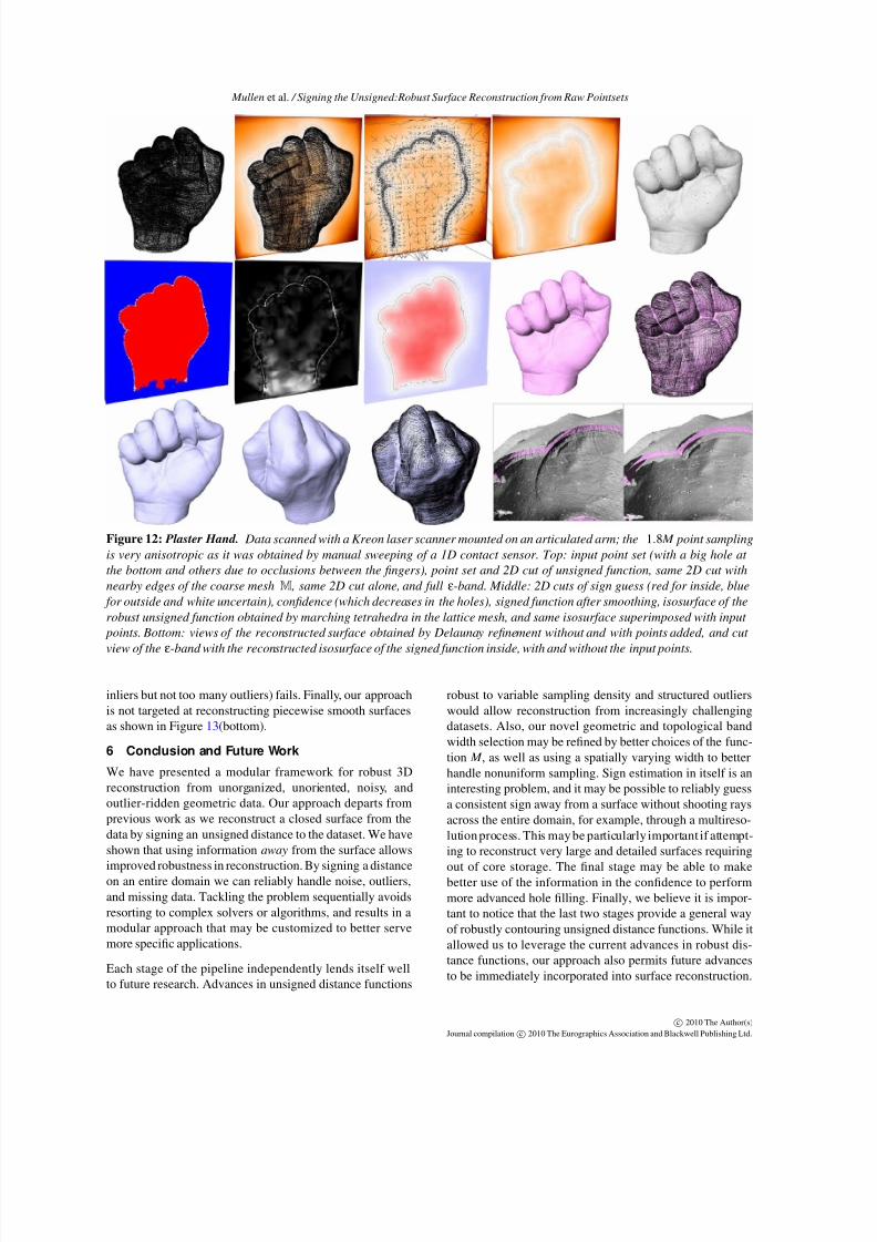
A typical example such as the hand in Figure 12, contain-ing 1.8M points and run with a depth of 9, took a total of

420 seconds. Of that time the KNN data structure construc-tion took 14s, the construction of M took 8.6s, the unsignedfunction computation took 3.7s, the analysis for finding εtook 31s, the sign guess took 181s, the smoothing outsidethe band took .3s, the refinement inside the band to get Mtook 127s, the sign propagation into the band took 37s, andthe final solve including computing the Laplacian matrix andperforming 30 Jacobi iterations took 80s. By far the longest


7/30/2019 MDDCA10



example was the elephant taking 4630s with a depth of 12 tocapture the very fine details, while the Caesar model was theshortest taking 350s with a depth of 9. We found the only pa-rameters we needed to play with were the depth of the meshM, generally taken between 8 and 12 based on the level of detail desired, and K generally ranging from 12 to 30 based

on the number of outliers. For our ray shooting we nevertook more than r = 20 rays per point. Examples of parame-ters used for our figures are given in the following table.

Model depth K #rays Time (s) El ephant 12 12 15 4,630Column 11 15 15 2,350 Indonesian lady 8 30 15 1,270 Hand 9 20 15 420Caesar 9 15 20 350

On dense, noise-free examples (Figure 8) our approach per-forms comparably to state-of-the-art reconstruction methodssuch as Poisson reconstruction [KBH06], although our cur-rent code cannot compare in terms of scalability with ad-

vanced implementations such as [BKBH07, MPS08]. Forsuch cases when normals are given or can be properly es-timated and oriented, the added value of our approach is thesimplicity and efficiency of the Jacobi iterations and its triv-ial parallelization.

Our approach is thus primarily targeted at dealing withthe cases where the point set comes with no attributesand the normal orientation and estimation algorithms (e.g.,[HDD∗92, AB99]) fail because of bad sampling conditions.On the hand model scanned with a Kreon laser scanner forexample (Figure 9), the anisotropic and noisy nature of thesampling made it impossible to properly orient the normals,and these failures are reflected in the reconstruction pro-duced by Poisson surface reconstruction. Our approach dealswith this dataset without issue.

The flexible lady model (Figure 10) and the column model(Figure 7) are also shown because they challenge conven-tional normal orienters. More specifically, the MST-basednormal orienter [HDD∗92] proceeds by constructing a graphover the K nearest neighbors and propagating a seed nor-mal orientation through a minimum spanning tree over thegraph. When the graph is disconnected the normals of dis-

Figure 9: Brittleness of Normal Orientation. On the highly

anisotropic and noisy hand scan from Figure 12 , normal ori-

entation fails at several places which translates into artifacts

when Poisson reconstruction [KBH06 ] is used.

Figure 10: Flexible Lady. Robust reconstruction from irreg-

ular sampling. Top: input point set, oriented normals (red

segments are normals where the orienter fails) and points

with unoriented normals. Bottom: our reconstructed isosur-

face with and without input points, and output of Poisson

reconstruction with same depth.

Figure 11: Indonesian Lady. Robust reconstruction from a

highly non-uniform pointset with no attributes.

connected regions cannot be properly oriented. Choosing alarger parameter K is a solution but it leads to the connec-tion of nearby surfaces of opposite orientations. Instead, ourapproach handles these datasets gracefully.

The robustness of our approach to outliers is illustrated onthe Caesar head model in Figure 3: the bottom figure hasadditional noise and 200K outliers, but our outlier-robustmethod still captures the shape quite well. Also, while therobust unsigned function is not designed to properly dealwith nonuniform sampling, our automatic band width com-putation combined with the use of a more accurate distanceinside of the band helps to handle very irregular sampling.

Figure 11 illustrates our approach on a model with a non-uniform sampling, taken from [HLZ∗09] for comparison.

Limitations. While the unsigned distance function hasproven robust to noise and outliers, the measure-based ap-proach does not deal well with structured outliers (i.e., out-liers with regular patterns, making them look like features).We see one such example in Figure 13(top), where the au-tomatic selection of the ε-band (which should enclose most


7/30/2019 MDDCA10



Figure 12: Plaster Hand. Data scanned with a Kreon laser scanner mounted on an articulated arm; the 1.8 M point sampling

is very anisotropic as it was obtained by manual sweeping of a 1D contact sensor. Top: input point set (with a big hole at

the bottom and others due to occlusions between the fingers), point set and 2D cut of unsigned function, same 2D cut with

nearby edges of the coarse mesh M , same 2D cut alone, and full ε-band. Middle: 2D cuts of sign guess (red for inside, blue

for outside and white uncertain), confidence (which decreases in the holes), signed function after smoothing, isosurface of the

robust unsigned function obtained by marching tetrahedra in the lattice mesh, and same isosurface superimposed with input

points. Bottom: views of the reconstructed surface obtained by Delaunay refinement without and with points added, and cut

view of the ε-band with the reconstructed isosurface of the signed function inside, with and without the input points.

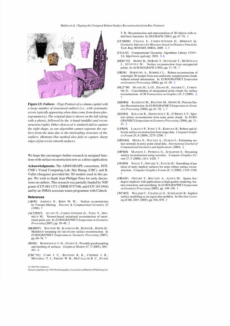
inliers but not too many outliers) fails. Finally, our approachis not targeted at reconstructing piecewise smooth surfacesas shown in Figure 13(bottom).

6 Conclusion and Future Work

We have presented a modular framework for robust 3Dreconstruction from unorganized, unoriented, noisy, andoutlier-ridden geometric data. Our approach departs fromprevious work as we reconstruct a closed surface from thedata by signing an unsigned distance to the dataset. We haveshown that using information away from the surface allows

improved robustness in reconstruction. By signing a distanceon an entire domain we can reliably handle noise, outliers,and missing data. Tackling the problem sequentially avoidsresorting to complex solvers or algorithms, and results in amodular approach that may be customized to better servemore specific applications.

Each stage of the pipeline independently lends itself wellto future research. Advances in unsigned distance functions

robust to variable sampling density and structured outlierswould allow reconstruction from increasingly challengingdatasets. Also, our novel geometric and topological bandwidth selection may be refined by better choices of the func-tion M , as well as using a spatially varying width to betterhandle nonuniform sampling. Sign estimation in itself is aninteresting problem, and it may be possible to reliably guessa consistent sign away from a surface without shooting raysacross the entire domain, for example, through a multireso-lution process. This may be particularly important if attempt-ing to reconstruct very large and detailed surfaces requiring

out of core storage. The final stage may be able to makebetter use of the information in the confidence to performmore advanced hole filling. Finally, we believe it is impor-tant to notice that the last two stages provide a general wayof robustly contouring unsigned distance functions. While itallowed us to leverage the current advances in robust dis-tance functions, our approach also permits future advancesto be immediately incorporated into surface reconstruction.


7/30/2019 MDDCA10



Figure 13: Failures. (Top) Pointset of a column capital with

a large number of structured outliers (i.e., with systematic

errors typically appearing when data come from dense pho-

togrammetry). The original data is shown on the left (along

with a photo), followed by the ε-band (middle) and recon-

struction (right). Other choices of ε similarly fail to capture

the right shape, as our algorithm cannot separate the out-

liers from the data due to the misleading structure of the

outliers. (Bottom) Our method also fails to capture sharp

edges of piecewise smooth surfaces.

We hope this encourages further research in unsigned func-tions with surface reconstruction now as a direct application.

Acknowledgments. The AIM@SHAPE consortium, ISTI-

CNR’s Visual Computing Lab, Hui Huang (UBC), and B.Vallet (Imagine) provided the 3D models used in this pa-per. We wish to thank Jean-Philippe Pons for early discus-sions on outliers. This research was partially funded by NSFgrants (CCF-0811373, CMMI-0757106, and CCF-1011944)and by an INRIA associate teams programme with Caltech.

References

[AB99] AMENTA N., BERN M. W.: Surface reconstructionby Voronoi filtering. Discrete & Computational Geometry 22(1999). 7

[ACSTD07] ALLIEZ P., COHEN-STEINER D., TONG Y., DES-BRUN M.: Voronoi-based variational reconstruction of unori-ented point sets. In EUROGRAPHICS Symposium on GeometryProcessing (2007), pp. 39–48. 2

[BKBH07] BOLITHO M., KAZHDAN M., BURNS R., HOPPE H.:Multilevel streaming for out-of-core surface reconstruction. In EUROGRAPHICS Symposium on Geometry Processing (2007),pp. 69–78. 7

[BO05] BOISSONNAT J.-D., OUDOT S.: Provably goodsamplingand meshing of surfaces. Graphical Models 67 , 5 (2005), 405–451. 6

[CBC∗01] CARR J . C. , BEATSON R. K. , CHERRIE J. B.,MITCHELL T. J., FRIGHT W. R., MCCALLUM B. C., EVANS

T. R.: Reconstruction and representation of 3D objects with ra-dial basis functions. In SIGGRAPH (2001), pp. 67–76. 1

[CCSM09] CHAZAL F., COHEN-STEINER D., MÉRIGOT Q.:Geometric Inference for Measures based on Distance Functions.Tech. Rep. 00383685, INRIA, 2009. 2, 3

[CGA10] Computational Geometry Algorithms Library CGAL-

3.6. http://www.cgal.org/, 2010. 3, 6[HDD∗92] HOPPE H., DEROSE T., DUCHAMP T., MCDONALD

J. , STUETZLE W.: Surface reconstruction from unorganizedpoints. In ACM SIGGRAPH (1992), pp. 71–78. 7

[HK06] HORNUNG A., KOBBELT L.: Robust reconstruction of watertight 3D models from non-uniformly sampled point cloudswithout normal information. In EUROGRAPHICS Symposiumon Geometry Processing (2006), pp. 41–50. 2

[HLZ∗09] HUANG H., LI D., ZHANG H., ASCHER U., COHEN-OR D.: Consolidation of unorganized point clouds for surfacereconstruction. ACM Transactions on Graphics 28 , 5 (2009). 2,7

[KBH06] KAZHDAN M., BOLITHO M., HOPPE H.: Poisson Sur-face Reconstruction. In EUROGRAPHICS Symposium on Geom-etry Processing (2006), pp. 61–70. 1, 7

[KSO04] KOLLURI R., SHEWCHUK J. R., O’BRIEN J. F.: Spec-tral surface reconstruction from noisy point clouds. In EURO-GRAPHICS Symposium on Geometry Processing (2004), pp. 11–21. 2

[LPK09] LABATUT P., PONS J.-P., KERIVEN R.: Robust and ef-ficient surface reconstruction from range data. Computer Graph-ics Forum 28 , 8 (2009), 2275–2290. 1

[MNG04] MITRA N., NGUYEN A., GUIBAS L.: Estimating sur-face normals in noisy point cloud data. International Journal of Computational Geometry and Applications (2004). 2

[MPS08] MANSON J., PETROVA G., SCHAEFER S.: Streamingsurface reconstruction using wavelets. Computer Graphics Fo-rum 27 , 5 (2008), 1411–1420. 7

[NOS09] NAGAI Y., OHTAKE Y., SUZUKI H.: Smoothing of par-tition of unity implicit surfaces for noise robust surface recon-

struction. Computer Graphics Forum 28 , 5 (2009), 1339–1348.1

[OBA05] OHTAKE Y., BELYAEV A., ALEXA M.: Sparse low-degree implicits with applications to high quality rendering, fea-ture extraction, and smoothing. In EUROGRAPHICS Symposiumon Geometry Processing (2005), pp. 149–158. 1

[WCS05] WALDER C., CHAPELLE O., SCHÖLKOPF B.: Implicitsurface modelling as an eigenvalue problem. In Machine Learn-ing ICML 2005 (2005), pp. 936–939. 2


MDDCA10

Documents

Transcript of MDDCA10