Md. Rahimul Hasan Asif Masters of Engineering …tariq/asif.pdf · •Centrifugal pump ......

Md. Rahimul Hasan Asif

Masters of Engineering Student

Memorial University of Newfoundland

• New faster dynamic modeling method for a remote hybrid

power system of Ramea, Newfoundland

• Simulation with the pumped hydro storage system

replacing current low efficiency hydrogen electrolyzer and

generator system

• Supervisory controller design with six case studies and

detailed simulation results

• Different operational modes of diesel engine generator to

estimate the fuel consumption, no of switching and system

frequency deviation

• Introduction

• Ramea hybrid power system

• Pumped hydro storage

• Dynamic Modeling: All subsystems

• Wind turbines: Northern Power 100 and Windmatic 15s

• Diesel engine generator

• Centrifugal pump

• Pelton wheel turbine

• Sealed Lead Acid Battery

• Electrical system and Supervisory controller

• Simulations for six extreme cases of wind speed and load

• Simulation results and analysis

• Diesel consumption analysis for high penetration system

• Simulation results and analysis

• Conclusion, Contribution and Future work

• Questions

• Ramea Hybrid Power System

• Pumped Hydro Storage

Ramea Island Newfoundland

• Ramea, Newfoundland and Labrador is a small village located on Northwest Island,

one of a group of five major islands located off the south coast of the island of

Newfoundland, Canada

• The Island is approximately 3.1 km long by 1 km wide

Components to

be removed

Existing hybrid power system Proposed hybrid power system with

pumped hydro storage

Components to

be added

Typical hydroelectric plant Pumped hydro

storage

Pumped water when wind speed is high or/and load demand is low

Bidirectional machine can be used to pump or generate but provides poor efficiency

A centrifugal pump coupled with induction motor can be used to pump water

Pelton wheel turbine is a good option as this system will rarely be operated at rated

flow and this turbine has high part flow efficiency

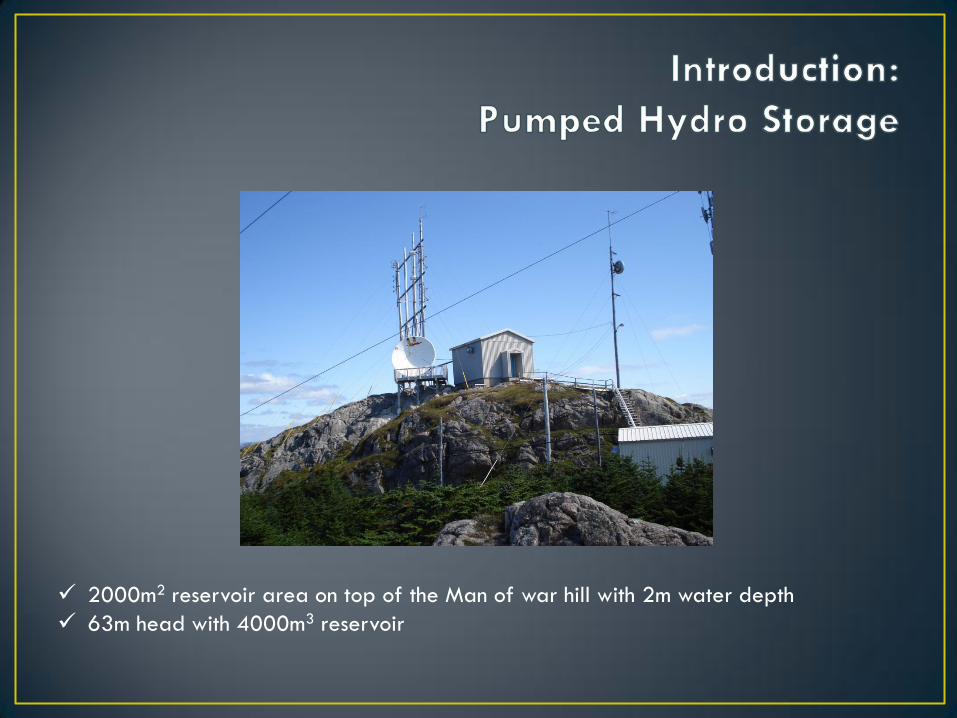
2000m2 reservoir area on top of the Man of war hill with 2m water depth

63m head with 4000m3 reservoir

Wind turbines, Diesel engine generator, centrifugal pump, Pelton wheel turbine, battery

Simulink - MATLAB embedded function block based dynamic model of Ramea hybrid

power system with pumped hydro storage, battery bank and controllable dump load

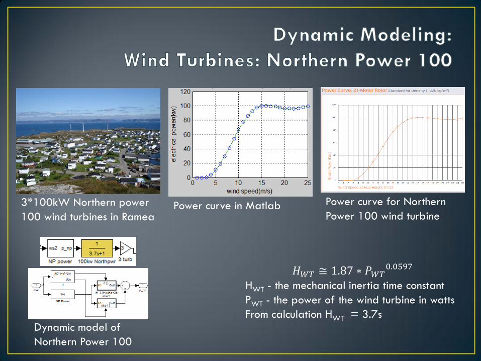
Power curve for Northern

Power 100 wind turbine

𝐻𝑊𝑇 ≅ 1.87 ∗ 𝑃𝑊𝑇0.0597

HWT - the mechanical inertia time constant

PWT - the power of the wind turbine in watts

From calculation HWT = 3.7s

3*100kW Northern power

100 wind turbines in Ramea Power curve in Matlab

Dynamic model of

Northern Power 100

Power curve for Windmatic

15s wind turbine

𝐻𝑊𝑇 ≅ 1.87 ∗ 𝑃𝑊𝑇0.0597

HWT - the mechanical inertia time constant

PWT - the power of the wind turbine in watts

From calculation HWT = 3.6s

3*100kW Windmatic 15s

wind turbines in Ramea Power curve in Matlab

Dynamic model of

Windmatic 15s

J =𝑆𝑛𝑇𝐷𝐸𝐺𝜔𝑛

2

J - the moment of inertia

ωn - the rated angular velocity

Sn - the DEG nominal apparent power

TDEG - the acceleration time constant for Sn

Here, J = 20kg.m2 results TDEG ≅ 2 s

Dynamic model of diesel generator

Frequency droop model

D = 2E-14*x^2 + 5E-08*x + 0.0101

Diesel consumption

measurement block and

function

Centrifugal pump coupled

with induction motor

Dynamic model of

pump and reservoir

Overall efficiency considering

all dynamic losses is 50%

Reynolds number

Re = 2000;

Darcy Friction Factor

flam=64/Re;

Darcy-Weisbach equation for head loss due to friction

hpipefric = (8*flam*Lpipe*qres^2)/(g*3.1416^2*Dpipe^5)

klossco is the loss coefficient for water meter

hlossmeter = klossco*(Velowaterpump^2)/(2*g)

Total dynamic head loss

Hloss = hpipefric + hlossmeter;

Operates from 30% to

100% of the rated value

Part flow efficiency of a

Pelton wheel turbine

Spare jet Pelton wheel turbine

Dynamic model of

Pelton wheel turbine 150kW Pelton wheel turbine

Overall efficiency is considered 70%

Operates from 30% to 100% of the rated value

Dynamic model of

battery bank

Charging

block

Battery

bank

Discharging

block

Individual capacity – 200Ahr

Battery per string – 20

Bus voltage – 240V DC (20*12V)

Number of string – 15

Number of battery – 300

Efficiency – 80%

• Maximum charging rate 10% of capacity

i.e. 72kW

• Maximum discharge rate 33% of capacity

i.e. 237.6kW

• For discharge rate higher than 20hr rate of

battery ‘Peukert's law’ is applied.

• This battery bank can response in millisecond

range

It = C𝐶

𝐼𝐻

𝑘−1

Dynamic model of

the Electrical System

Dynamic model

of the

Supervisory

controller

Electrical System • M - System inertia constant (0.2)

• D - Load-damping constant (0.012)

• 0.05pu (5%) power deviation in grid

will cause 0.01pu (1%) or 0.6Hz

frequency deviation

Supervisory Controller • In left side all are input parameters from the

component blocks

• In right side all are output parameters to the

component blocks

• Algorithm is implemented inside this block with C

code

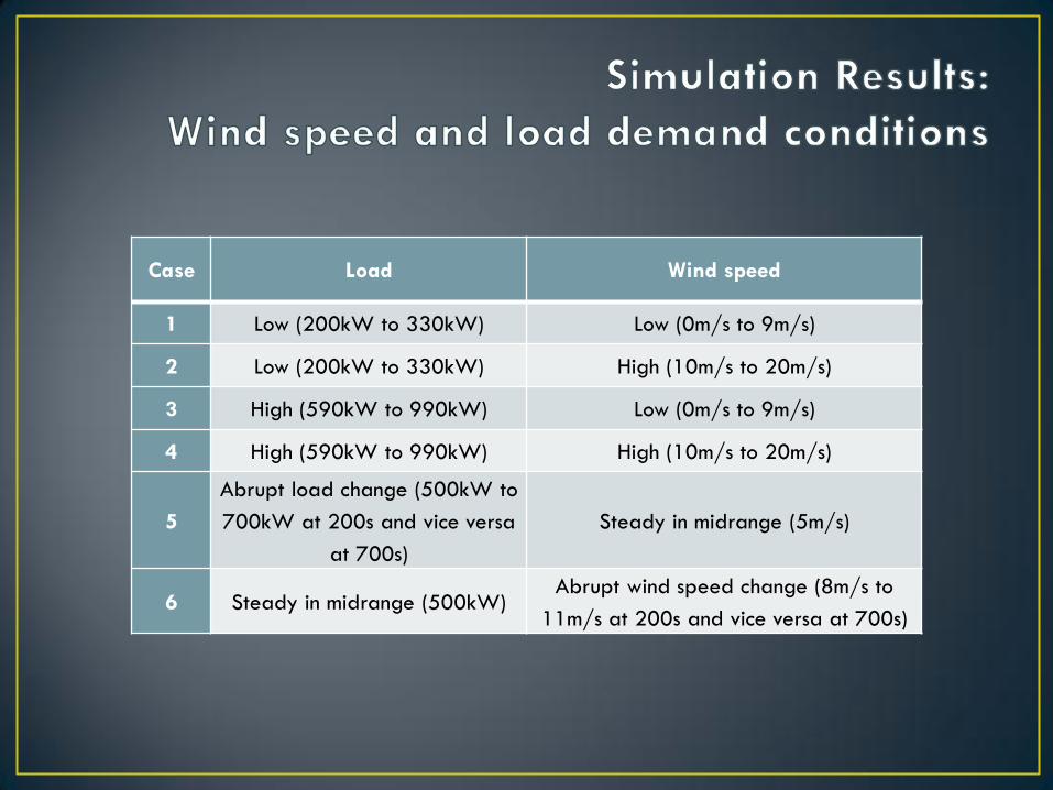
Case Load Wind speed

1 Low (200kW to 330kW) Low (0m/s to 9m/s)

2 Low (200kW to 330kW) High (10m/s to 20m/s)

3 High (590kW to 990kW) Low (0m/s to 9m/s)

4 High (590kW to 990kW) High (10m/s to 20m/s)

5

Abrupt load change (500kW to

700kW at 200s and vice versa

at 700s)

Steady in midrange (5m/s)

6 Steady in midrange (500kW) Abrupt wind speed change (8m/s to

11m/s at 200s and vice versa at 700s)

Low (200kW to 330kW) Low (0m/s to 9m/s) 1.3Hz

Load demand (kW) and wind speed

(m/s) data for the case 1

Grid available power (kW) and DEG

varying output (kW) (with a

minimum 300kW value) is shown

and in the lower figure dump

power (kW) is shown for the case 1

Pump power consumption (kW),

pump water flow (m3/s), the upper

reservoir water volume (m3),

turbine water flow rate (m3/s) and

the turbine generated power (kW)

for the case 1

Low (200kW to 330kW) Low (0m/s to 9m/s) 1.3Hz

Grid surplus power (kW) with and

without pumped storage, battery

and dump load and the resultant

frequency deviation for the case 1

BB charging current (kA), charging

power (kW), percentage of state of

charge, discharging current (kA)

and the power to the grid (kW) due

to the discharging of the battery

are shown for the case 1

Simulation result has been

zoomed from 57700s to 57800s to

show the transients. In top figure,

the grid available power (kW) and

DEG varying output (kW) is shown

and in the lower figure the

resultant frequency deviation is

shown for the case 1

Low (200kW to 330kW) High (10m/s to 20m/s) ~0Hz


(m/s) data for case 2 In the top part, grid available

power (kW) and DEG output (kW)

(with flat 300kW value) are shown

and in the lower part dump power

(kW) is shown for the case 2

Pumping power (kW), pumping

water flow rate (m3/s), upper

reservoir water volume (m3),

turbine water flow (m3/s) and

turbine generated power (kW) for

the case 2

Low (200kW to 330kW) High (10m/s to 20m/s) ~0Hz

BB charging current (kA), charging

power (kW), percentage of state of

charge, discharging current (kA) and the

power injected to the grid (kW) due to the

discharging of the battery are shown

above for the case 2


without pumped storage, battery and

dump load and the resultant frequency

deviation are shown above for the case 2

High (590kW to 990kW) Low (0m/s to 9m/s) 0.9Hz

Load demand (kW) and wind speed (m/s)

data for the case 3 In top figure, grid available power (kW)

and DEG varying output (kW) (from 400kW

to 925kW) are shown and in the bottom

part dump power (kW) is shown for the

case 3

Pumping power (kW), pumping water flow

(m3/s), upper reservoir water volume (m3),

turbine water flow (m3/s) and turbine

generated power (kW) are shown for the

case 3

High (590kW to 990kW) Low (0m/s to 9m/s) 0.9Hz

Charging current (kA), charging power (kW),

percentage of state of charge, discharging

current (kA) and injected power to the grid (kW)

due to the discharging of the battery are for the

case 3

Grid surplus power (kW) with and without

pumped storage, battery and dump load and the

resultant system frequency deviation for the case

3

High (590kW to 990kW) High (10m/s to 20m/s) 0.4Hz


(m/s) data for the case 4 In top figure grid available power

(kW) and DEG output (kW) (flat

300kW value) are shown and in the

lower part dump power (kW) is



water flow (m3/s), upper reservoir

water volume (m3), turbine water

flow (m3/s) and turbine generated

power (kW) for the case 4 are

shown above

High (590kW to 990kW) High (10m/s to 20m/s) 0.4Hz

Charging current (kA), charging power

(kW), percentage of state of charge,

discharging current (kA) and the power

injected to the grid (kW) due to the

discharging of the battery are shown




dump load are shown above. The

resultant frequency deviation is also

plotted for the case 4



at 700s)


0.2Hz



In top part, grid available power (kW) and

DEG varying output (kW) (that changes

from 300kW to 500kW) are shown. In the

lower part dump load power (kW) is

plotted for the case 5

Pumping power (kW), pumping water flow

(m3/s), upper reservoir water volume (m3),

turbine water flow (m3/s) and turbine

generated power (kW) are plotted above

for the case 5



at 700s)


0.2Hz

BB charging current (kA), charging power (kW),

percentage of state of charge, discharging

current (kA) and injecting power to the grid (kW)

due to the discharging of the battery are plotted


The grid surplus power (kW) with and without

pumped storage, battery and dump load and

the resultant frequency deviation for the case 5

Steady in midrange (500kW) Abrupt wind speed change (8m/s to


1.1Hz



In the top part, grid available

power (kW) and DEG varying

output (kW) (with a flat 300kW) and

in bottom part dump power (kW) is



water flow (m3/s), upper reservoir

water volume (m3), turbine water

flow (m3/s) and turbine generated

power (kW) are shown above for

the case 6

Steady in midrange (500kW) Abrupt wind speed change (8m/s to


1.1Hz

Charging current (kA), charging power

(kW), percentage of state of charge,

discharging current (kA) and injected

power to the grid (kW) due to the

discharging of the battery are plotted




dump resistance and the resultant

frequency deviation are shown above for

the case 6

Case Load Wind speed

Maximum

frequency

deviation

1 Low (200kW to 330kW) Low (0m/s to 9m/s) 1.3Hz

2 Low (200kW to 330kW) High (10m/s to 20m/s) ~0Hz

3 High (590kW to 990kW) Low (0m/s to 9m/s) 0.9Hz

4 High (590kW to 990kW) High (10m/s to 20m/s) 0.4Hz

5



at 700s)


0.2Hz

6 Steady in midrange (500kW) Abrupt wind speed change (8m/s to


1.1Hz

• For all conditions system frequency remain in acceptable range

• This deviations sustain for brief period only

Simulation result and analysis

MODES DEG operation mode

Mode 1 Always ON

Mode 2 ON/OFF

Continuous control

Mode 3 Minimum 10 min after

last switching over

Load demand data and Wind

speed data for one day (86400s),

average wind speed 4.9ms-1 and

load 303kW

The grid available power (kW) and DEG output

(kW) (with a minimum 300kW value) is shown

and in the lower figure dump power (kW) is

shown for mode 1

Pump power consumption (kW), pump water flow

(m3/s), the upper reservoir water volume (m3),

turbine water flow rate (m3/s) and the turbine

generated power (kW) for the Mode 1


percentage of state of charge, discharging current

(kA) and the power to the grid (kW) due to the

discharging of the battery are shown for the mode

1



resultant frequency deviation for the mode 1

Grid available power (kW) and DEG output (kW)

are shown and in the lower part dump power (kW)

is shown for the mode 2

Pumping power (kW), pumping water flow rate

(m3/s), upper reservoir water volume (m3), turbine

water flow (m3/s) and turbine generated power (kW)

for the mode 2



(kA) and the power injected to the grid (kW) due to

the discharging of the battery are shown above

for the mode 2



resultant frequency deviation are shown above for

the mode 2

Grid available power (kW) and DEG output (kW) are shown and in the lower part the resultant

frequency deviation (Hz) are shown for the continuous control of DEG in Mode 2

Gives better system stability and consume almost same fuel as diesel ON/OFF mode

Can be achieved by using a variable speed diesel with an AC-DC-AC link

Grid available power (kW) and DEG output (kW)

(with flat 300kW value) are shown and in the lower

part dump power (kW) is shown for the mode 3

Pumping power (kW), pumping water flow rate

(m3/s), upper reservoir water volume (m3), turbine

water flow (m3/s) and turbine generated power

(kW) for the mode 3



(kA) and the power injected to the grid (kW) due to

the discharging of the battery are shown above

for the mode 3



resultant frequency deviation are shown above for

the mode 3

MODES DEG operation mode Diesel Intake

(Liter)

Maximum

Frequency

deviation (Hz)

No. of

Switching

Mode 1 Always ON 2323 -1.5 0

Mode 2 ON/OFF 1866 -7 Many

Continuous control 2039 -0.15 0

Mode 3 Minimum 10 min after last

switching over 2110 -10 Less

Faster simulation with simpler but detailed dynamic model

and intelligent supervisory controller is possible • A computer with Intel Core2Duo 2.1GHz processor and 4GB RAM takes only

30minutes to simulate any case for one day (86400 seconds)

• 1st order transfer function with all characteristics and dynamic losses

Analyses for all extreme cases could be done • Comprehensive case studies can be done with this dynamic model

• Analysis on different operational modes of diesel engine generator and their

fuel consumption can be done

Modified control of DEG is required for high penetration of

wind energy • Intelligent supervisory controller is required for complicated control strategies

to operate the diesel engine generator

Novel method for dynamic modeling • Customized Simulink function blocks have been used

• Built-in Simulink blocks can be used with this function blocks

Compatibility and flexibility • For future extension of the hybrid system this model can be modified easily

• Different wind speed and load data can be used

• This model can be used to justify feasibility of a pumped hydro storage in a hybrid

power system for a different location

• Changing any components requires only change on that particular block

• With adequate resources this model is able to simulate longer period of time e.g. few

months to year

Supervisory controller design and simulation • Algorithm to control each components based on the capabilities, needs and priorities

• Complicated operation for diesel OFF high penetration operation

Further development by integrating higher order models • Simulation time will increase considerably

• May give better performance of the system and provide opportunity to analysis

higher order transient responses.

AC voltage and reactive power analysis • AC transient behavior e.g. phase angle, reactive power can be analyzed

• Integration of synchronous condenser or variable capacitors can be done using

• Controls of such system will be more complicated

Other types of dynamic controllers • Fuzzy logic, neural network etc. can be used here as a future work to study

possible improvement to the transient behavior of this model.

This model can be experimented for other remote hybrid power

systems and a detailed environmental impact analysis and

economic analysis can also be done

• Dr. Tariq Iqbal

• The NSERC Wind Energy Strategic Network (WESNet); funded

by industry and the Natural Sciences and Engineering Research

Council of Canada (NSERC)

• School of Graduate Studies of MUN

• Faculty of Engineering and Applied Science of MUN

• My family and friends

• Paper published in the conference proceedings and presented

in the IEEE Newfoundland Electrical and Computer Engineering

Conference 2012, St. John’s, Newfoundland and Labrador,

Canada

• Poster presented on 3rd WESNet and CanWEA (Canadian wind

Energy Association) poster sessions 2012

• Paper accepted for publishing in the International Journal of

Energy Science (IJES)

• Paper accepted for presentation and publishing in the

conference IEEE Electrical Power and Energy Conference 2013,

Halifax, Nova Scotia, Canada.

Md. Rahimul Hasan Asif Masters of Engineering …tariq/asif.pdf · •Centrifugal pump ......

Documents

Transcript of Md. Rahimul Hasan Asif Masters of Engineering …tariq/asif.pdf · •Centrifugal pump ......