1 © IWA Publishing 2018 Water Science & Technology | in press | 2018

Uncorrected Proof

A comparative study of manhole hydraulics using

stereoscopic PIV and different RANS models

Md Nazmul Azim Beg, Rita F. Carvalho, Simon Tait, Wernher Brevis,

Matteo Rubinato, Alma Schellart and Jorge Leandro

ABSTRACT

Flows in manholes are complex and may include swirling and recirculation flow with significant

turbulence and vorticity. However, how these complex 3D flow patterns could generate different

energy losses and so affect flow quantity in the wider sewer network is unknown. In this work, 2D3C

stereo Particle Image Velocimetry measurements are made in a surcharged scaled circular manhole.

A CFD model in OpenFOAM® with four different Reynolds Averaged Navier Stokes (RANS) turbulence

model is constructed using a volume of fluid model, to represent flows in this manhole. Velocity

profiles and pressure distributions from the models are compared with the experimental data in view

of finding the best modelling approach. It was found among four different RANS models that the RNG

k-ε and k-ω SST gave a better approximation for velocity and pressure.

doi: 10.2166/wst.2018.089

Md Nazmul Azim Beg (corresponding author)Rita F. CarvalhoDepartment of Civil Engineering,University of Coimbra,Coimbra,PortugalE-mail: mnabeg@uc.pt

Simon TaitWernher BrevisMatteo RubinatoAlma SchellartDepartment of Civil and Structural Engineering,University of Sheffield,Sheffield, UK

Wernher BrevisDepartment of Hydraulics and EnvironmentalEngineering,

Pontifical Catholic University of Chile,Santiago, Chile

Jorge LeandroHydrology and River Basin Management,Technical University of Munich,Munich, Germany

Key words | manhole, OpenFOAM®, RANS model, stereoscopic PIV, VOF

INTRODUCTION

Manholes are one of themost common features in urban drai-

nage networks. They are located at changes in slope andorientation of the sewer pipes, as well as at regular intervalsalong the pipes to enable maintenance. The flow pattern in

a manhole is complex, especially during high flows, andinvolves several hydraulic phenomena such as local flowcon-traction, expansion, rotation, recirculation as well as possible

air entrainment and sediment mixing. These flow phenom-ena can control the overall energy loss, transport anddispersion of solute and particulate materials in the manholestructure. PIV measurement can provide a good represen-

tation of the complex velocity field of a manhole.Previously Lau () studied two-dimensional PIV in a sur-charged scaled manhole. Attempts to measure stereo PIV

data in a scaledmanhole are however newand to the authors’knowledge, has not been done before. Several researchersstudied flow patterns in surcharged manholes using CFD

models. Use of different Reynolds Averaged Navier Stokes(RANS) modelling approach like RNG k-ε model (Lau

et al. ), Realizable k-ε (Stovin et al. ), k-ω model

(Djordjevic et al. ) have been reported. A little researchstudy has been conducted on how these flow patterns couldaffect flowmovement and flow quality in the wider piped net-

work. In the current work, the flow phenomena of a scaledmanhole are measured by stereo Particle Image Velocimetry(PIV) and modelled numerically using OpenFOAM® CFD

tools. Four different RANS models, i.e. RNG k-ε, Realizablek-ε, k-ω SST and Launder-Reece-Rodi (LRR) were used, andthe differences in flow structures among them were com-pared and discussed.

METHODS AND MATERIALS

Experimental model

The experimental facility was installed in the Hydraulic Lab-oratory of the University of Sheffield. It consists of a

2 M. N. A. Beg et al. | Comparison of manhole hydraulics using PIV and different RANS model Water Science & Technology | in press | 2018

Uncorrected Proof

transparent acrylic circular scaled manhole, linked to a

model catchment surface (Rubinato et al. ). The man-hole has an inner diameter (Φm) of 240 mm andconnected with a 75 mm diameter (Φp) inlet-outlet pipes.

Both pipes are co-axial, and the pipe axis passes throughthe centre of the manhole vertical axis (Figure 1). Two but-terfly valves (one at >48Φp upstream the manhole, theother one at >87Φp downstream the manhole) are used to

control the inflow and the water depth of the manholerespectively. The inflow was monitored using an electromag-netic MAG flow meter fitted within the inlet sewer pipe

(10Φp from the butterfly inlet valve). The ratio of the man-hole diameters to inlet pipe diameters (Φm/Φp) is 3.20.Two Gems series pressure sensors (Product code

5000BGM7000G3000A, serial number 551362, range0–70 mb) were installed vertically at the inlet and outletpipes, the first one at 350 mm upstream from the centrelineof the manhole, the second one, 520 mm downstream from

the centreline of the manhole by making a hole in the pipeof Φ¼ 5 mm. They can measure piezometric pressures forboth free surface and pressure flow conditions within the

inlet-outlet pipes. These transducers were calibrated suchthat transducer output signal (4–20 mA) can be directlyrelated to gauge pressure. For the calibration of the pressure

Figure 1 | Experimental setup for 2D3C stereo PIV measurement at the manhole.

transmitter 10 different water levels were measured (range

50 to 500 mm, no discharge) and checked with a pointgauge. Rubinato () found an overall accuracy can bedefined as ±0.72 mm. A transparent measuring tape was

attached vertically to the manhole side in order to checkthe manhole water levels during the experiments. The tapeposition was at the other side of the camera, keeping anequal distance from both inlet and outlet.

PIV measurement

A stereo PIV measurement setup was installed. Two Dantec

FlowSense EO 2M cameras and an Nd:YAG pulsed laserwas placed at opposite sides of the scaled manhole. Eachcamera resolution was 1,600 × 1,200 pixels (Figure 1) andwas set at the same distance from the manhole making

more than 45� angle at the vertical centre of the measuringplane. To reduce error due to refraction through the curvedmanhole wall, a transparent acrylic tank was constructed

around it and filled with water, keeping flat surfaces parallelto both camera lens axes. The laser was directed from thebottom of the acrylic manhole as a laser sheet with the

help of a flat mirror set at 45� to the horizontal direction.The laser sheet thickness was around 4 mm.

3 M. N. A. Beg et al. | Comparison of manhole hydraulics using PIV and different RANS model Water Science & Technology | in press | 2018

Uncorrected Proof

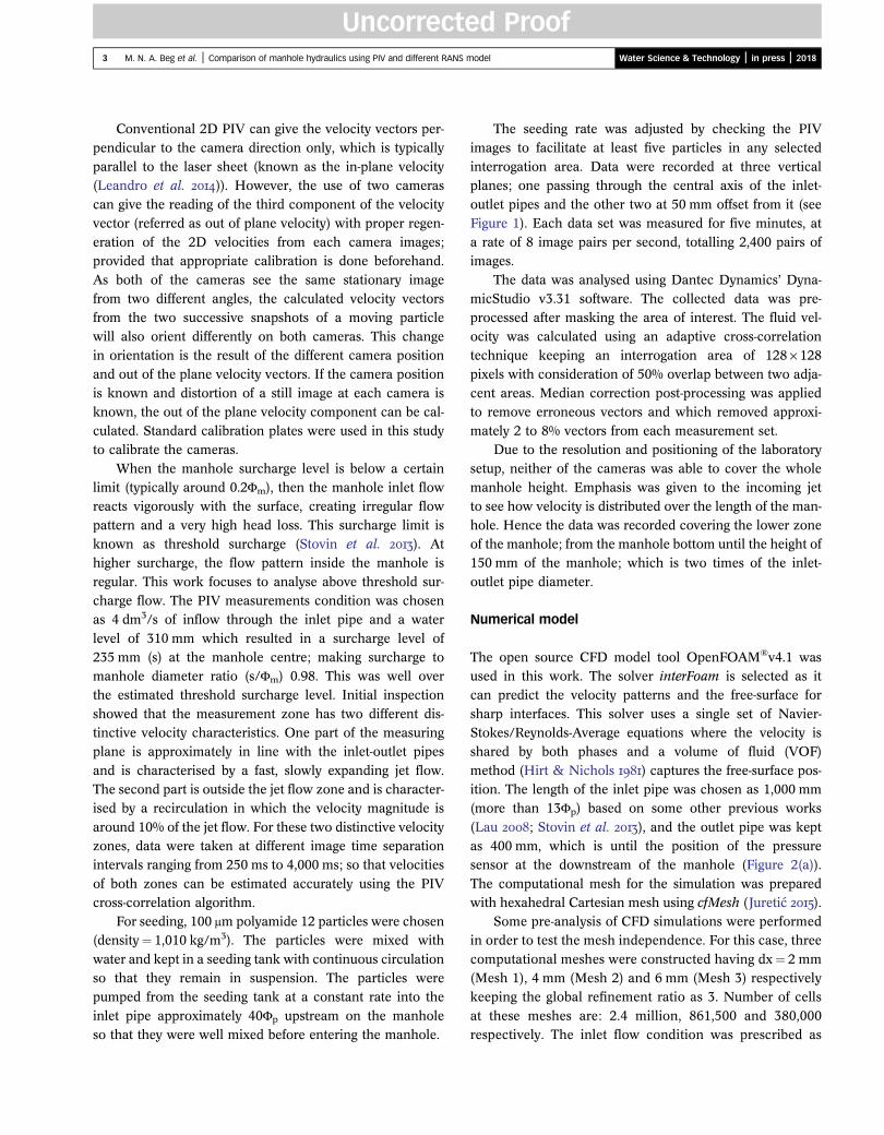
Conventional 2D PIV can give the velocity vectors per-

pendicular to the camera direction only, which is typicallyparallel to the laser sheet (known as the in-plane velocity(Leandro et al. )). However, the use of two cameras

can give the reading of the third component of the velocityvector (referred as out of plane velocity) with proper regen-eration of the 2D velocities from each camera images;provided that appropriate calibration is done beforehand.

As both of the cameras see the same stationary imagefrom two different angles, the calculated velocity vectorsfrom the two successive snapshots of a moving particle

will also orient differently on both cameras. This changein orientation is the result of the different camera positionand out of the plane velocity vectors. If the camera position

is known and distortion of a still image at each camera isknown, the out of the plane velocity component can be cal-culated. Standard calibration plates were used in this studyto calibrate the cameras.

When the manhole surcharge level is below a certainlimit (typically around 0.2Φm), then the manhole inlet flowreacts vigorously with the surface, creating irregular flow

pattern and a very high head loss. This surcharge limit isknown as threshold surcharge (Stovin et al. ). Athigher surcharge, the flow pattern inside the manhole is

regular. This work focuses to analyse above threshold sur-charge flow. The PIV measurements condition was chosenas 4 dm3/s of inflow through the inlet pipe and a water

level of 310 mm which resulted in a surcharge level of235 mm (s) at the manhole centre; making surcharge tomanhole diameter ratio (s/Φm) 0.98. This was well overthe estimated threshold surcharge level. Initial inspection

showed that the measurement zone has two different dis-tinctive velocity characteristics. One part of the measuringplane is approximately in line with the inlet-outlet pipes

and is characterised by a fast, slowly expanding jet flow.The second part is outside the jet flow zone and is character-ised by a recirculation in which the velocity magnitude is

around 10% of the jet flow. For these two distinctive velocityzones, data were taken at different image time separationintervals ranging from 250 ms to 4,000 ms; so that velocities

of both zones can be estimated accurately using the PIVcross-correlation algorithm.

For seeding, 100 μm polyamide 12 particles were chosen(density¼ 1,010 kg/m3). The particles were mixed with

water and kept in a seeding tank with continuous circulationso that they remain in suspension. The particles werepumped from the seeding tank at a constant rate into the

inlet pipe approximately 40Φp upstream on the manholeso that they were well mixed before entering the manhole.

The seeding rate was adjusted by checking the PIV

images to facilitate at least five particles in any selectedinterrogation area. Data were recorded at three verticalplanes; one passing through the central axis of the inlet-

outlet pipes and the other two at 50 mm offset from it (seeFigure 1). Each data set was measured for five minutes, ata rate of 8 image pairs per second, totalling 2,400 pairs ofimages.

The data was analysed using Dantec Dynamics’ Dyna-micStudio v3.31 software. The collected data was pre-processed after masking the area of interest. The fluid vel-

ocity was calculated using an adaptive cross-correlationtechnique keeping an interrogation area of 128 × 128pixels with consideration of 50% overlap between two adja-

cent areas. Median correction post-processing was appliedto remove erroneous vectors and which removed approxi-mately 2 to 8% vectors from each measurement set.

Due to the resolution and positioning of the laboratory

setup, neither of the cameras was able to cover the wholemanhole height. Emphasis was given to the incoming jetto see how velocity is distributed over the length of the man-

hole. Hence the data was recorded covering the lower zoneof the manhole; from the manhole bottom until the height of150 mm of the manhole; which is two times of the inlet-

outlet pipe diameter.

Numerical model

The open source CFD model tool OpenFOAM®v4.1 wasused in this work. The solver interFoam is selected as itcan predict the velocity patterns and the free-surface for

sharp interfaces. This solver uses a single set of Navier-Stokes/Reynolds-Average equations where the velocity isshared by both phases and a volume of fluid (VOF)

method (Hirt & Nichols ) captures the free-surface pos-ition. The length of the inlet pipe was chosen as 1,000 mm(more than 13Φp) based on some other previous works

(Lau ; Stovin et al. ), and the outlet pipe was keptas 400 mm, which is until the position of the pressuresensor at the downstream of the manhole (Figure 2(a)).

The computational mesh for the simulation was preparedwith hexahedral Cartesian mesh using cfMesh (Juretic ).

Some pre-analysis of CFD simulations were performedin order to test the mesh independence. For this case, three

computational meshes were constructed having dx¼ 2 mm(Mesh 1), 4 mm (Mesh 2) and 6 mm (Mesh 3) respectivelykeeping the global refinement ratio as 3. Number of cells

at these meshes are: 2.4 million, 861,500 and 380,000respectively. The inlet flow condition was prescribed as

Figure 2 | (a) Numerical model mesh (top left panel), (b) Boundary locations (top right panel) and (c) Mesh convergence test (bottom panel).

4 M. N. A. Beg et al. | Comparison of manhole hydraulics using PIV and different RANS model Water Science & Technology | in press | 2018

Uncorrected Proof

constant discharge of Q¼ 4 dm3/s. The meshes were simu-lated using k-ε turbulence model and the velocity profiles atthe manhole centre and at the outlet pipe were extracted

from the results (Figure 2(c)). The mesh analysis was per-formed applying Richardson extrapolation (Celik et al.). The meshes gave similar results at the manhole jet

zone and at the pipe. However, the velocity profilesshowed different results closed to the manhole water sur-face (at around z¼ 0.29 m to 0.31 m) and close to thebottom (around z¼ 0 m). Mesh 3 predicted slightly slower

velocity at the near surface zone. The apparent order (p)and the Grid Convergence Index (GCI) was calculated ateach grid point of the meshes. The average value of p at

the manhole centre and pipe were found 2.76 and 2.32respectively. The GCI values were found higher close to

the surface and the walls. Analysis showed that 50% cellsin the manhole has GCI value below 10% when comparingMesh 2 and Mesh 3; while 65% cell showed below 10%

GCI in case of comparing Mesh 1 and Mesh 2. However,in case of results at the pipe, 70% and 76% cells showedGCI value below 10% in case of comparing Mesh 3-Mesh

2 and Mesh 2-Mesh 1 respectively. It was apparent thatthe results go towards mesh independence and Mesh 1and Mesh 2 show almost similar results. Average approxi-mate relative error between Mesh 2 and Mesh 1 was

found to be 2.7%, whereas the simulation time requirementfor Mesh 1 was more than three times to that of Mesh2. Considering the accuracy level and computational time

required, Mesh 2 with dx¼ 4 mm was found best suitedfor this work.

5 M. N. A. Beg et al. | Comparison of manhole hydraulics using PIV and different RANS model Water Science & Technology | in press | 2018

Uncorrected Proof

The model considers all the manhole borders as noSlipwall (i.e. zero velocity at the wall) and three open bound-aries: inlet, outlet and atmosphere (Figure 2(b)). Wallroughness was not considered as the aim was to character-

ize the flow velocity patterns in the manhole in which thewall energy losses were considered small in comparisonwith the entry, exit and mixing losses. The inlet boundaryconditions were prescribed as fixed velocity approving for

fully developed pipe flow profile using inverse power lawof pipe flow (Çengel & Cimbala , chap. 8):

vr ¼ vmax 1� rR

� �1=n(1)

where vr is the longitudinal velocity at a radial distance of rfrom the pipe axis, R is the pipe radius, vmax is the maximumlongitudinal velocity at the developed profile section and n isa constant which is dependent on the Reynold’s number of

the flow. To find the best combination of vmax and n, pre-analy-sis was done considering a pipe flow CFD model. The pipediameter was made the same as the inlet pipe (Φp¼ 0.075 m)and pipe length was kept 3 m (40 Φp). The model was simu-

lated using k-ε model applying the same inflow (Q¼ 4 dm3/s).It was found that the pipe becomes fully turbulent at flowreach of 27Φp (2 m length) and after 20 s of simulation

time. It produces vmax ¼ 1.128 ms�1 at fully turbulent con-dition and n¼ 6.5 gives the best fit curve of thedevelopment profile. These values were chosen to calculate

inlet boundary condition of the manhole model usingEquation (1). The outlet boundary condition was prescribedas fixed pressure boundary corresponding to average water

column pressure head, measured with the outlet pipepressure sensor (shown in Figure 1). The pressure at atmos-phere boundary condition (at the manhole top, shown atFigure 2(b)) was prescribed as equal to atmospheric pressureand zeroGradient for velocity to have free air flow, ifnecessary.

The mentioned condition was simulated with four differ-

ent Reynolds Average Navier-Stokes (RANS) turbulencemodelling approaches; namely: RNG k-ε model, Realizablek-εmodel, k-ω SST model and LRR model to evaluate if they

are able to characterize the flow properly. The first twomodels use a two-equation based approach calculating tur-bulent kinetic energy (k) and turbulent energy dissipation(ε). These two models are and formulated by Yakhot et al.() and Shih et al. () and known to be better thanthe standard k-ε model to give better prediction at separ-ating flow and spreading rate of round jets respectively.

The k-ω SST model used in OpenFOAM is based on

Menter & Esch () with updated coefficients from

Menter et al. () and addition of the optional F3 termfor rough walls (Hellsten ). This model uses rate of dis-sipation (ω) instead of ε at the near wall zone and standard

k-εmodel at the zones far from the wall influence and is sup-posed to give better prediction at the near wall andturbulence separating flow. Wall-functions are applied inthis implementation by using Kolmogorov-Prandtl

expression for eddy viscosity (Hellsten ) to specify thenear-wall omega as appropriate. The blending functionsare not currently used in OpenFOAM version because of

the uncertainty in their origin. The effect is considered neg-ligible in case of small yþ cell at the wall (Greenshields )and hence can be applied to models with low yþ cells. The

fourth model uses the seven equation based Reynolds StressModel (RSM); using turbulent kinetic energy (k) and sixcomponent of stress tensor (R) directly and therefore maypredict complex interactions in turbulent flow fields in a

better way. The initial condition was prescribed as fillingthe manhole up to the expected level. Inlet pipe, outletpipe and the manhole zone in line with the inlet-outlet

pipe was initialized with a fully developed velocity profilewhich was same as the inlet boundary condition. The inletturbulent boundary and initial conditions k, ε, R and νtwere calculated using standard equations as follows:

k ¼ 32

I uref

�� ��� �2(2)

ϵ ¼ C0:75μ k1:5

L(3)

νt ¼ Cμk2

ϵ(4)

ω ¼ k0:5

CμL(5)

where uref is the velocity to be considered, I is the turbulentintensity (chosen as 0.05 at this case), Cμ is a constant(¼0.09) and L is the characteristic length of the inlet pipe.

Standard wall function was considered in k-ω SSTmodel only as according to the model description, it requireswall function for yþ>1. The rest of the models require wall

function when 30< yþ<300.During the simulations, the adjustableRunTime code

was used keeping maximum Courant–Friedrichs–Lewy

(CFL) number to 0.95. Cluster computing system at the

6 M. N. A. Beg et al. | Comparison of manhole hydraulics using PIV and different RANS model Water Science & Technology | in press | 2018

Uncorrected Proof

University of Coimbra was used to run the simulations using

MPI mode. Each simulation was run for 65 seconds. Thesteady condition was ensured by checking the residuals ofp, alpha.water, k, epsilon and Rxx (where applicable). The

first 60 seconds were required to reach steady state con-dition and the results of 101 velocity profiles in the last 5seconds were averaged and all the numerical analysis weremade using averaged data of these mentioned time step

results.

RESULTS AND DISCUSSION

The processed PIV velocity data were compared with vel-

ocity data of the manhole model. The PIV measurementwas taken at the central vertical plane (CVP) along withthe left vertical plane (LVP) and right vertical plane (RVP)

(Figure 1). However, the position of LVP was much furtherfrom the camera, and light ray coming from the two edges ofthe LVP have to travel through the manhole inlet-outletpipe. Although the scaled manhole model is made of trans-

parent acrylic, the joints between the model componentswere semi-transparent to non-transparent. Due to this limit-ation, the LVP image edges had bad data in some cases, as

the camera could not see the seeding particles due to theobstruction made by the model joints. So in this work,PIV data comparison is only done to the CVP and RVP of

the manhole. Figure 3 shows the axial (Vx) and vertical(Vz) velocity components comparison between the PIVdata and numerical model results. All the comparison isshown as dimensionless velocities as a ratio of the average

inlet velocity (Vavg), where Vavg is the ratio between inlet dis-charge (Q) and pipe cross section (Ap). Both PIV data andCFD data are showing temporal mean velocities from the

measurements and simulation results. PIV data at the CVPnear the manhole inlet and outlet pipe were not collectedas it was not visible clearly by the cameras due to the

joints between pipe and manhole.It can be seen from the velocity comparison at the CVP

of PIV (1st and 3rd column of row 1 at Figure 3), that the jet

flow in the experimental results starts expanding slowly as itproceeds from the inlet towards the outlet. The CVP axialvelocity (Vx) (1st column of Figure 3) reaches up to 110%of Vavg at the experimental results. It dampens down at

the manhole centre. The maximum velocity near the outletpipe is the same as Vavg. However, in the CFD data, thisdamping effect is not seen. The high-velocity core stays as

110% of Vavg until it reaches the outlet. While the jet flowtrying to escape through the outlet pipe, it hits the manhole

wall at the top of the outlet (near x¼�100 mm and y¼75 mm) and creates a vertically upward velocity componentwhich is up to 20% of Vavg (3rd column of Figure 3). How-ever, in all the CFD, the vertical velocity component at this

zone reaches up to 30% of Vavg. Comparing the velocity con-tours of Vx and Vz at the CVP, it can be seen that LRR modelcould not predict the velocity profile properly. This modelshows different axial velocity contour at CVP which is dis-

similar to PIV measurements.Comparing the velocity towards the pipe axis at the RVP

(2nd column of Figure 3), RNG k-ε and Realizable k-ε

models slightly underestimate the axial velocity componentin compared to the PIV experiment. The PIV data showedaxial velocity up to 0.3 Vavg whereas, in these two numerical

models, the highest velocity is found 0.25 Vavg. The axial vel-ocity at this plane is properly estimated by k-ω SST model.The shape of the velocity contour is almost similar to thatof the PIV data. The vertical velocity component (Vz) (4th

column of Figure 3), at PIV is observed between �0.2 Vavg

and 0.2 Vavg. The numerical models show similar results ofVz near the outlet of the manhole. However, at the upper

part of the measuring plane near the inlet, the Vz wasmeasured in PIV as around �0.2 Vavg, which was not pre-dicted by the numerical models. Only k-ω SST model in

this plane shows a negative (downward) velocity near theinlet, however still underestimated than the PIV.

The velocity comparison was not done for out of the

plane component (Vy) as at CVP, this component is veryclose to zero and considered not significant (Figure 4).

The standard deviation of the data was also compared atboth CVP and RVP for axial and vertical velocity com-

ponents (Figure 5). The comparison was also made ondimensionless velocities as a ratio of Vavg.

It can be seen that for axial velocity component (Vx) at

CVP and RVP (1st and 2nd column at Figure 5), the PIVdata shows high standard deviation near inlet, outlet and jetexpansion zones. High standard deviation can also be seen

near the manhole floor of CVP. Vertical velocity component(Vz) showed lower deviation compared to Vx. The standarddeviation was found to be significantly low at both planes in

CFD results in compared to PIV data. All CFD results showmarginally higher standard deviation values close to the jetexpansion zone. The Realizable k-ε model shows the mini-mum fluctuation in the velocity fields, resulting almost zero

standard deviation. The k-ω SSTmodel shows the highest stan-darddeviation amongall the fourRANSmodels, still, the valueis lower than that of the PIV data. As these numerical models

are formulated from RANS equations, a big part of the turbu-lence variabilities is averaged out from the results already.

Figure 3 | Comparison of non-dimensional velocity components from the numerical models and PIV measurement at both CVP and RVP of the manhole. The flow direction is from right to

the left.

7 M. N. A. Beg et al. | Comparison of manhole hydraulics using PIV and different RANS model Water Science & Technology | in press | 2018

Uncorrected Proof

Perhaps Large Eddy Simulation (LES) model could showbetter standard deviation match with the PIV data. Moreover,

for this work, only 5 seconds of numerical simulation datawasconsidered. In case the longer period of data was taken intoconsideration, probably the standard deviation in the CFD

results would come higher. Turbulence coming from piperather than the standard turbulence inlet conditions couldalso be a reason for the differences in numeric.

Examining the velocity contours at Figures 3 and 5, it

can be stated that k-ω SST model creates the closest approxi-mation of the manhole velocity field followed by RNG k-εmodel. The LRR model overestimates the axial velocity com-

ponent in this plane and the velocity contour is significantlydifferent than the PIV measurement.

To understand themanhole flowmore clearly, streamlineand water level fluctuation was analysed from the numerical

model results (Figure 6). It can be seen that the inflow jet orig-inating from the inlet, marginally spread in the manhole(termed as the diffusive region). When exiting the manhole

through the outlet pipe, the diffusive region impinges themanhole wall and after that part of the jet flow moves verti-cally upward. This flow region reaches the manhole watersurface, starts moving opposite to the core jet direction and

makes a clockwise circulation. Due to this constant circula-tion, the free surface of the manhole fluctuates slightly. Thefluctuation was foundmore towards the inlet of the manhole.

In this case, the water level was observed varying between0.295 m to 0.320 m. The fluctuation level was found different

Figure 4 | Out of the plane velocity component at the CVP from PIV and four RANS models.

8 M. N. A. Beg et al. | Comparison of manhole hydraulics using PIV and different RANS model Water Science & Technology | in press | 2018

Uncorrected Proof

in the four numerical models. In RNG k-ε model, the waterlevel varies from 0.300 m to 0.310 m. While the water level

fluctuations in the other three manhole models were foundas Realizable k-ε: varying between 0.300 m and 0.305 m; k-ω SST: varying between 0.300 m and 0.310 m and LRR: vary-ing between 0.310 m and 0.320 m. In the experimental work

the average water level at the manhole was observed as0.310 m. The fluctuation of the manhole level was not poss-ible to measure in the experimental work as it would

require installing a pressure sensor at the manhole bottom,which would create an obstacle in the laser ray path lineand hence was not used.

The pressure distributions in different CFD modelswere also compared with experimental data and can beseen in Figure 7. All distances showed at the horizontal

axis are measured from the manhole centre. The inletand outlet pipes are connected at distance of 0.12 m and�0.12 m respectively. The bottom pressure in betweenthese two distances also represents free surface water

level inside the manhole. Two box plots represent pressuredata recorded during the experimental measurement usingpressure sensors. The left box plot shows the pressure at

the outlet pipe, whose average value was used to generateboundary condition of the numerical models. As the

downstream pressure is same for all the four models, allthe model results pass through the average value of this

box. Pressures at the upstream side were calculated fromthe models. All the line plots are showing maximum, mini-mum and average bottom pressure from each of the fourCFD models. The circular marker at the manhole centre

(at x¼ 0 m) is showing the product of recorded averagewater height at the manhole during the experimentalworks (h¼ 0.310 m), water density (ρ) and gravitational

acceleration (g).From Figure 7, it can be seen that when the upstream

flow through the inlet pipe enters the manhole, the flow

experiences a pressure drop, which is due to the expansionof the flow. The second pressure drop can be observed whenthe flow exits the manhole and enters the outlet pipe. This

drop is due to the flow contraction and much bigger in mag-nitude. The average pressure line of RNG k-ε, Realizable k-εand k-ω SST models produce a similar pressure patternthroughout the computational domain. The LRR model

overestimates the bottom pressure of the manhole, althoughthe difference found is in the range of few millimetres ofwater column head. The maximum, minimum and the aver-

age bottom pressure from RNG k-ε model shows almost thesame line which presents that the RNG k-ε model shows

Figure 5 | Temporal standard deviation of different velocity component at CVP and RVP, measured from PIV data and four RANS models.

9 M. N. A. Beg et al. | Comparison of manhole hydraulics using PIV and different RANS model Water Science & Technology | in press | 2018

Uncorrected Proof

almost zero pressure fluctuation. Apparently, the LRRmodel overestimated the pipe loss in compared to the

other three models. This results in an overestimation ofupstream pressure at the inlet direction.

The coefficient of head loss (K) in the manhole is known

as the ratio between head loss and the velocity head and iscalculated using Equation (6).

K ¼ ΔH=v2

2g

� �(6)

where ΔH is the head loss, v is the average longitudinal vel-ocity at the outlet pipe (¼0.89 m/s) and g is the accelerationdue to gravity.

As the numerical model reached steady state beforeextracting any results, and as both inlet and outlet pipes

were full, the temporal averaged velocity at each pipe canbe considered equal. In this case, a difference in bottompressure would give the same value as head loss. To com-

pute the pressure drop at the manhole centre for a certainCFD result, each line showing the average bottom pressure(Figure 7) was projected to the manhole centre from bothinlet and outlet pipe. The vertical difference of pressure

value between these two lines at the manhole centre givesthe value of pressure drop for the manhole, which is laterdivided by ρg and considered as ΔH.

The value of manhole head loss coefficient has beenreported in different literature. This is directly related to

Figure 6 | Flow streamline through the manhole and water level range from different models.

Figure 7 | Bottom pressure comparison from different RANS models and the experimental pressure sensor data.

10 M. N. A. Beg et al. | Comparison of manhole hydraulics using PIV and different RANS model Water Science & Technology | in press | 2018

Uncorrected Proof

the structural mould types of the manhole, manhole to pipe

diameter ratios, as well as manhole surcharge ratio. A com-parable analysis of the coefficients of head loss (K) with

those of the values reported in different literature are

shown in Table 1. It should be noted that only the researchworks reporting the same manhole mould type are

Table 1 | Different values of head loss coefficient (K) at different models

Works done Head loss coefficient Experimental condition (Φm/Φp)

Surcharge ratio range

s/Φm s/Φp

Marsalek () 0.210 1.923

Arao & Kusuda () 0.18–0.58 3.60 0.55–1.67 2–6

Lau et al. () 0.28–0.69 9.08 0.65–0.82 5.90–7.45

This work

RNG k-ε 0.193 3.20 0.98 3.13

Realizable k-ε 0.156

k-ω SST 0.284

LRR 0.265

11 M. N. A. Beg et al. | Comparison of manhole hydraulics using PIV and different RANS model Water Science & Technology | in press | 2018

Uncorrected Proof

considered here. In the work of both Arao & Kusuda ()and Lau et al. (), authors reported high head loss coeffi-

cient at below threshold surcharge conditions andcomparably lower coefficient at above threshold surchargecondition. As in this research, the manhole surcharge con-dition is comparable to above threshold surcharge, only

the coefficient range covering this condition are shown.Table 1 shows that the four models calculate the man-

hole flow differently and hence give different values of

manhole head loss coefficient. It is reported by differentauthors the head loss coefficient becomes higher when man-hole to pipe diameter ratio (Φm/Φp) is high and vice versa

(Bo Pedersen & Mark ; Stovin et al. ). The manholereported at Arao & Kusuda () has a similar Φm/Φp.Comparing the findings from the literature, it is apparentthe Realizable k-ε model gives rather low head loss coeffi-

cient for this case. From the rest three models, thecoefficient given by k-ω SST model is almost 50% morethan that of value given by RNG k-ε, however, both values

lie within the range specified by other researchers.

CONCLUSIONS

In this work, two-dimensional three component (2D3C)

stereo PIV measurement was done on a scaled inline man-hole with manhole to pipe diameter ratio of 3.20, in orderto evaluate CFD model constructed in OpenFOAM® andfour different RANS models with VOF method. From the

analysis, it can be apparent that each model calculates thevelocity inside manhole differently. Comparison with PIVmeasurement at the CVP showed similar velocity as com-

pared to all the numerical models. However, comparisonof the velocity at another vertical plane 50 mm offset to

the centre, showed that all the CFD models slightly under-predicts the axial velocity. The velocity and locations of

vortex structures centres were found marginally differentamong the models. The k-ω SST model showed the closestapproximation of velocity contour followed by the RNGk-εmodel. All the models showed very good approximations

of the average water surface level at the manhole. However,the LRR model could not quite capture the velocity profilein compared to PIV data. This model predicts considerably

higher axial velocities for CVP as compared to PIV. None-theless, the temporal standard deviations of the axial andvertical velocity components were found significantly low

when compared to those of experimental measurementthrough PIV. As a RANS model is formulated based ontime-averaged turbulence data, which could be the reasonof having a lower standard deviation in the CFD model.

Bottom pressure analysis through the computationaldomain shows that the average pressure line is almost simi-lar at RNG k-ε, Realizable k-ε and k-ω SST models.

However, the comparison could be made with data fromonly two pressure sensors installed at the inlet and outletpipe respectively. RNG k-ε model showed almost no

pressure fluctuation while maximum pressure line predictedby the Realizable k-εmodel was found much higher than themeasurement. The calculated head loss coefficients were

compared with the values reported in the literature. It wasseen that the Realizable k-ε model shows much lowervalue compared to the values reported.

Considering all the aspects of the four models analysed

here, it can be said that both RNG k-ε model and k-ω SSTmodels give a very good approximation of manhole hydrau-lics. However, it should be noted while using k-ω SST model,

the wall boundary cell size must be made considerably smallfor the proper formulation of the model.

12 M. N. A. Beg et al. | Comparison of manhole hydraulics using PIV and different RANS model Water Science & Technology | in press | 2018

Uncorrected Proof

ACKNOWLEDGEMENTS

The work presented is part of the QUICS (Quantifying

Uncertainty in Integrated Catchment Studies) project. Thisproject has received funding from the European Union’sSeventh Framework Programme for research, technologicaldevelopment and demonstration under grant agreement No.

607000. The laboratory facility was made possible throughEPSRC, project EP/K040405/1. All the numerical resultshere showed were performed on the Centaurus Cluster of

the Laboratory for Advanced Computing of University ofCoimbra, Portugal.

REFERENCES

Arao, S. & Kusuda, T. Effects of pipe bending angle on energylosses at two-way circular drop manholes. In: 8thInternational Conference on Urban Storm Drainage. Sydney,Australia, 8th International Conference on Urban StormDrainage, pp. 2163–2168.

Bo Pedersen, F. & Mark, O. Head losses in sewer manholes:submerged Jet Theory. Journal of Hydraulic Engineering116 (11), 1317–1328.

Celik, I. B., Ghia, U., Roache, P. J., Freitas, C. J., Coleman, H. &Raad, P. E. Procedure for estimation and reporting ofuncertainty due to discretization in CFD applications.Journal of Fluids Engineering 130 (7), 78001.

Çengel, Y. A. & Cimbala, J. M. Fluid Mechanics (S. Jeans,ed.). McGraw-Hill, New York, USA.

Djordjevic, S., Saul, A. J., Tabor, G. R., Blanksby, J., Galambos, I.,Sabtu, N. & Sailor, G. Experimental and numericalinvestigation of interactions between above and belowground drainage systems. Water Science and Technology67 (3), 535–542.

Greenshields, C. J. OpenFOAM User Guide v5.0.Hellsten, A. Some Improvements in Menter’s k-omega-SST

turbulence model. In: 29th AIAA Fluid DynamicsConference, Albuquerque, New Mexico, U.S.A., pp. 1–11.

Hirt, C. W. & Nichols, B. D. Volume of fluid (VOF) methodfor the dynamics of free boundaries. Journal of

Computational Physics 39 (1), 201–225. [online] http://www.sciencedirect.com/science/article/pii/0021999181901455.

Juretic, F. cfMesh User Guide (v1.1). Zagreb, Croatia.Lau, S. D. Scaling Dispersion Processes in Surcharged

Manholes. PhD Thesis, Department of Civil and StructuralEngineering, University of Sheffield, UK.

Lau, S. D., Stovin, V. R. & Guymer, I. The prediction ofsolute transport in surcharged manholes using CFD. WaterScience and Technology 55 (4), 57–64.

Lau, S.-T. D., Stovin, V. R. & Guymer, I. Scaling the solutetransport characteristics of a surcharged manhole. UrbanWater Journal 5 (1), 33–42. [online] http://www.tandfonline.com/doi/abs/10.1080/15730620701737249.

Leandro, J., Bung, D. B. & Carvalho, R. Measuring voidfraction and velocity fields of a stepped spillway forskimming flow using non-intrusive methods. Experiments inFluids 55 (5).

Marsalek, J. Energy Losses at Straight-Flow-Through SewerJunctions. Ontario, Canada.

Menter, F. & Esch, T. Elements of Industrial heat transfer. In:16th Brasilian Congress of Mechanical Engineering(COBEM). Uberlândia, Brasil, COBEM, pp. 117–127.

Menter, F. R., Kuntz, M. & Langtry, R. Ten Years ofIndustrial Experience with the SST Turbulence Model. In:Turbulence Heat and Mass Transfer 4 (K. Hanjalic, Y.Nagano & M. Tummers, eds). Begell House, Inc., Antalya,Turkey, pp. 625–632.

Rubinato, M. Physical Scale Modelling of Urban FloodSystems. PhD Thesis, Department of Civil and StructuralEngineering, University of Sheffield, UK.

Rubinato, M., Martins, R., Kesserwani, G., Leandro, J., Djordjevic, S.& Shucksmith, J. Experimental calibration and validationof sewer/surface flow exchange equations in steady andunsteady flow conditions. Journal of Hydrology 552, 421–432.

Shih, T.-H., Liou, W. W., Shabbir, A., Yang, Z. & Zhu, J. A new k-e eddy viscosity model for high Reynolds numberturbulent flows. Compurers Fluids 24 (3), 227–238.

Stovin, V. R., Bennett, P. & Guymer, I. Absence of a hydraulicthreshold in small-diameter surcharged manholes. ASCEJournal of Hydraulic Engineering 139 (September), 984–994.

Yakhot, V., Thangam, S., Gatski, T. B., Orszag, S. A. & Speziale,C. G. Development of Turbulence Models for ShearFlows by A Double Expansion Technique. Hampton,Virginia.

First received 24 October 2017; accepted in revised form 16 February 2018. Available online 28 February 2018