MCNP6 CODE DEVELOPMENT FOR ONE DIMENSIONAL POSITION

SENSITIVE THERMAL NEUTRON DETECTORS

A Thesis

by

JOSEPH G. FUSTERO

Submitted to the Office of Graduate and Professional Studies of

Texas A&M University

in partial fulfillment of the requirements for the degree of

MASTER OF SCIENCE

Chair of Committee, Ryan G. McClarren

Co-Chair of Committee, Delia Perez-Nunez

Committee Members, Marvin L. Adams

Daniel G. Melconian

Head of Department, Yassin A. Hassan

December 2017

Major Subject: Nuclear Engineering

Copyright 2017 Joseph G. Fustero

ii

ABSTRACT

The development of position sensitive thermal neutron detectors (PSD’s) began

soon after the initial development of early model thermal neutron detectors. One

dimensional (1D) PSD’s report not only neutron counts but the axial position of the

neutron interaction within the detector gas volume. These detectors maintain a high level

of fidelity except when the neutron interaction takes place close to the gas-shell

boundary.

The use of PSD’s in order to characterize the spatial distribution of the thermal

neutron field will become more commonplace as the technology has become less

expensive. These experiments, however, must be validated against simulation results in

order to assure their quality. The stochastic radiation transport code MCNP6 was used in

order to provide these simulation results due to its large user base and its compatibility

with the Parallel Deterministic Transport (PDT) code.

It was found that it is possible to use MCNP6 to accurately simulate 1D PSD’s

without heavily editing the source code. MCNP6 was used to simulate both the position

of the neutron interaction as well as the predicted detector response due to the charge

generation resultant of this interaction. This was done by writing a TALLYX

modification to the default energy deposition F6 tally for charged particles which result

from a neutron interaction. Additionally, it was found that using the PTRAC particle

tracing utility for events contributing to the F6 tally for the cell corresponding to the

detector gas volume was also appropriate for determining the location of the neutron

iii

interaction and the corresponding detector response due to charge collection on the

anode wire.

These simulations were run for a line detector test problem, a modified already

completed impurity model experiment, and a future localized source experience. For all

of these simulations the expected spatial distribution (including symmetries) and notable

physical features (wall effect due to surface leakage of heavy charged particles) was

observed. The computational expense did not differ significantly from a simulation using

the default MCNP6 tallies.

iv

DEDICATION

This thesis is dedicated to Michael Crichton who can be blamed for inspiring the

naive author of this thesis to pursue a career in science and engineering.

v

ACKNOWLEDGEMENTS

I would like to thank Dr. McClarren for his patience while advising me on this

project. As a newcomer to computational science, I often posed questions that would

seem obvious to the more experienced mind, yet he would always take the time to

address my concerns in detail.

I would also like to thank Dr. Thomas Conroy and Dr. Sophit (Bo) Pongpun, the

experimentalists working with our group’s position sensitive detector. Our numerous

conversations offered me insight into how to accurately model all of the physical

phenomena which contribute to the experimental detector response.

Additionally, I would like to thank Dr. Adams for initially proposing this project

and providing some of the initial assumptions. And I would like to thank the other

members of my committee, Dr. Melconian and Dr. Perez-Nunez for their feedback and

questions throughout the process of performing this research.

Finally, I would like to thank Kermit Bunde (Department of Energy) for assisting

me in compiling MCNP6 using modern compilers.

vi

CONTRIBUTORS AND FUNDING SOURCES

Contributors

This work was supported by a thesis committee of Dr. Ryan McClarren

[advisor], Dr. Delia Perez-Nunez [co-advisor], and Dr. Marvin Adams of the Department

of Nuclear Engineering and Dr. Daniel Melconian of the Department of Physics.

Insightful discussions with Dr. Thomas Conroy and Dr. Sophit Pongpun both of

the Texas A&M Engineering Experiment Station helped with developing Chapter 3.

Additional discussions with Kermit Bunde of the Department of Energy served as

precursors to the code development outlined in Chapter 4.

All other work conducted for the thesis was completed by the student

independently.

Funding Sources

This project was funded by the Center for Exascale Radiation Transport (CERT).

CERT was founded by a grant from the National Nuclear Security Agency (NNSA),

specifically under the Predictive Science Academic Alliance Program (PSAAP-II).

vii

NOMENCLATURE

CERT Center for Exascale Radiation Transport

HCP Heavy Charged Particle

MCNP Monte Carlo n-Particle

PSD Position Sensitive Detector

SR Stopping Range

SRIM Stopping Range of Ions in Matter

viii

TABLE OF CONTENTS

Page

1. INTRODUCTION………………………………………………………………........ 1

2. CHARGED PARTICLE PHYSICS…………………………………………………. 2

3. CURRENT TECHNOLOGY………………………………………………………... 5

3.1 Position Sensitive Detectors…………………………………………………. 10

3.2 MCNP6: Stochastic Radiation Transport……………………………………. 15

4. METHODOLOGY…………………………………………………………………. 19

4.1 PTRAC………………………………………………………………………. 20

4.2 TALLYX…………………………………………………………………….. 32

5. TEST PROBLEMS AND RESULTS………………………………………………. 35

5.1 Line Detector………………………………………………………………… 37

5.2 Modified Localized Source Experiment……………………………………... 40

5.3 Modified Impurity Model (IM-1) Experiment………………………………. 44

6. CONCLUSIONS…………………………………………………………………… 48

REFERENCES…………………………………………………………………………. 49

ix

LIST OF FIGURES

FIGURE Page

3.1 Sketch (not from an actual detector) neutron energy spectrum for a finite

BF3 detector. Reprinted from [9]………………………………………….. 7

3.2 Physical representation of the resultant HCP’s traveling through the

BF3 detection medium. Reprinted from [9]……………………………….. 7

3.3 Neutron reaction cross sections for 19

F. Reprinted from [14]…………….. 8

3.4 Neutron reaction cross sections for 10

B. Reprinted from [14]…………….. 8

3.5 Schematic for a gamma photon PSD. Reprinted from [10]………………. 12

4.1 Example PTRAC file with designated particle events separated into

blocks by source particle number. Reprinted from [7]…………………… 21

4.2 Energy of a 1.78 MeV alpha particle traversing BF3…………………….. 22

4.3 Energy of a 1.47 MeV alpha particle traversing BF3…………………….. 22

4.4 Energy of a 1.02 MeV lithium ion traversing BF3……………………….. 23

4.5 Energy of a 0.84 MeV lithium ion traversing BF3……………………….. 24

4.6 Ion damage results with SRIM for 1.78 MeV alpha particles in BF3.

Longitudinal range is 18.0 mm………………………………………….... 25

4.7 Ion damage results with SRIM for 1.47 MeV alpha particles in BF3.

Longitudinal range is 14.9 mm…………………………………………… 26

4.8 Ion damage results with SRIM for 1.02 MeV 7Li ions in BF3.

Longitudinal range is 9.49 mm…………………………………………… 26

4.9 Ion damage results with SRIM for 0.84 MeV 7Li ions in BF3.

Longitudinal range is 8.44 mm…………………………………………… 26

5.1 Counts and counting error results for all three methods (line detector)….. 37

5.2 Counts difference between the two PTRAC methods (line detector)……. 38

x

5.3 TALLYX curve fitting results (line detector)……………………………. 39

5.4 BF3 gas detector (much lower density than the simulations in Section

4.1) wrapped with an aluminum shell and wrapped in cadmium with

a slit in the central portion of the tube. Reprinted from [16]……………… 40

5.5 Counts and counting error results for all three methods

(localized source)…………………………………………………………. 41

5.6 Counts difference between the two PTRAC methods (localized source)… 42

5.7 TALLYX curve fitting results (localized source)……………………….... 43

5.8 A representative example of an IM-1 experiment. Reprinted from [13]…. 44

5.9 Counts and counting error results for all three methods (IM-1)………….. 45

5.10 Counts difference between the two PTRAC methods (IM-1)…………… 46

5.11 TALLYX curve fitting results (IM-1)……………………………………. 47

xi

LIST OF TABLES

TABLE Page

4.1 SR as predicted from each of the three methods…………………………. 29

1

1. INTRODUCTION

The Texas A&M CERT research group has recently acquired a 3 m long position

sensitive BF3 thermal neutron detector. This detector will be eventually taken to the

Nuclear Science Center in order to perform experiments characterizing the spatial

distribution of the thermal neutron flux coming from an AmBe neutron source.

In order to provide assurance that the results acquired by the experimentalists are

reasonable, it was decided that a computational analogue be created. MCNP6 was

chosen as the software to use in order to design this analogue. MCNP6 is a stochastic

radiation transport code that offers several key advantages. First, the author of this thesis

already had a working knowledge of the code from his background. Additionally,

MCNP6 allows for user modification of the source code and redistribution of these

changes through the use of patches. MCNP6 has a user base numbering in the tens of

thousands and thus patches and third party tools developed in order to create the

computational analogue can be used by others [5] [6]. MCNP6 has been used to model

PSD’s but only for efficiency and not position data [12]. Finally, a code such as

GEANT4 may also be useful in terms of its ability to model position sensitive detectors

as it has already been used in modeling the position response for gamma photon

detectors [10]; however, the Texas A&M computational group is also developing a

deterministic radiation transport code, Parallel Deterministic Transport (PDT). This code

can interpret the geometry and material specifications from MCNP6 input files. Thus,

for the sake of consistency, MCNP6 was selected as the modeling code.

2

2. CHARGED PARTICLE PHYSICS

Neutrons are not directly measurable by current radiation detection systems.

Such systems rely upon the collection of electrons produced during an interaction in

order to generate an electrical signal. However, neutrons do not directly ionize the

medium they are traveling through. Thus, electron production must occur due to the

production of secondary radiation due to a neutron interaction within the detection

medium. If this secondary radiation is charged, then electron production will occur.

While photons are neutral particles, they can directly ionize the detection medium

through the photoelectric effect.

Neutral and charged particles differ in several important ways. If a charged

particle with some initial energy is traveling through a medium, it will eventually lose all

of its energy and come to a stop. The distance it travels in the medium is known as the

stopping range (SR). On the other hand, neutral particles undergo what is known as

exponential attenuation. If monoenergetic neutral particles travel through a detection

medium, they all will not stop at the same distance. Rather, there will be a distribution of

distances where the neutral particle is stopped.

There are also differences between the transport of electrons and heavy charged

particles (HCP’s). Electrons are much less massive than heavier charged particles, with a

mass difference typically on the order of 10-4

. This results in electrons having curved

trajectories while traveling through a medium. Each Columbic interaction can so

strongly alter the trajectory of an electron such that they do not travel in straight lines.

3

On the other hand, HCP’s traveling through a medium do (on average) travel in straight

lines. While a few HCP’s will be scattered off at some angle (the Rutherford gold foil

experiment demonstrated this, thus showing the existence of the nucleus), almost all of

them will end up traveling in a straight line as the Columbic interactions they undergo

will change their momentum much less compared to the impulse received by electrons

[8]. This result will be important for later and will be confirmed by using MCNP6 and

the Stopping Range of Ions in Matter (SRIM) code in Section 4.

In general (for non-relativistic particles), the stopping power of a HCP can

modeled as [8]:

dE

dr⃗=

4πk02z2e4n

mV2l n (

2mV2

I). (2.1)

Where E is the energy of the heavy charged particle, r⃗ is the position of the heavy

charged particle, k0 is Coulomb’s constant, z is atomic number of the HCP, e is the

charge of an electron, n is the number density of electrons in the medium, m is the mass

of an electron, V is the velocity of the heavy charged particle, and I is the mean

excitation energy. From Eq. (2.1) it becomes obvious that the stopping power is

dependent on material properties as the function includes both the electron number

density and the mean excitation energy. Eq. (2.1) can also be written with several

correction terms for relativistic particles and corrections due to the HCP having electrons

(shell corrections) which are incorporated into MCNP. However, for the purpose of this

project, non-relativistic HCP’s will be assumed and Eq. (2.1) is valid. Since the particles

are non-relativistic, Eq. (2.1) can be further simplified:

4

dE

dr⃗=

2πk02z2e4nM

mEln (

4mE

IM). (2.2)

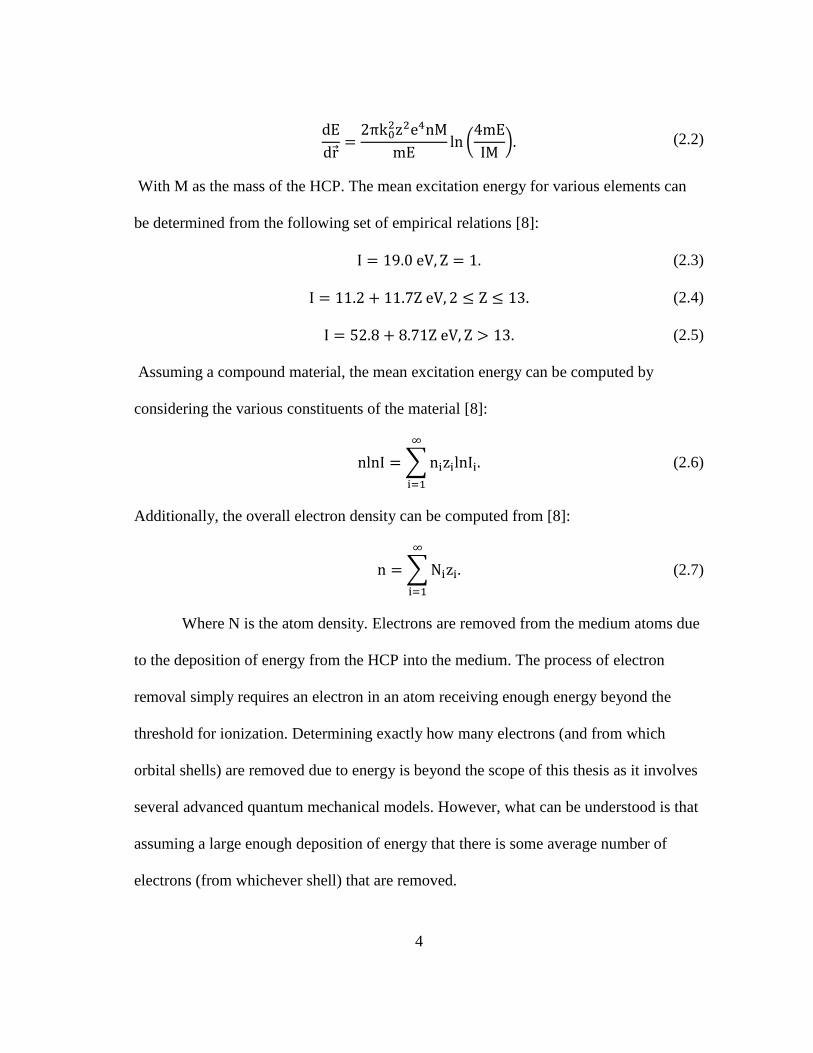
With M as the mass of the HCP. The mean excitation energy for various elements can

be determined from the following set of empirical relations [8]:

I = 19.0 eV, Z = 1. (2.3)

I = 11.2 + 11.7Z eV, 2 ≤ Z ≤ 13. (2.4)

I = 52.8 + 8.71Z eV, Z > 13. (2.5)

Assuming a compound material, the mean excitation energy can be computed by

considering the various constituents of the material [8]:

nlnI = ∑nizilnIi

∞

i=1

. (2.6)

Additionally, the overall electron density can be computed from [8]:

n = ∑Nizi

∞

i=1

. (2.7)

Where N is the atom density. Electrons are removed from the medium atoms due

to the deposition of energy from the HCP into the medium. The process of electron

removal simply requires an electron in an atom receiving enough energy beyond the

threshold for ionization. Determining exactly how many electrons (and from which

orbital shells) are removed due to energy is beyond the scope of this thesis as it involves

several advanced quantum mechanical models. However, what can be understood is that

assuming a large enough deposition of energy that there is some average number of

electrons (from whichever shell) that are removed.

5

3. CURRENT TECHNOLOGY

Neutron detection technologies have been around for decades [1]. Some of the

first neutron detectors were gas-filled cylinders. These detectors are still used for several

reasons. Thermal neutrons have a high interaction probability with the gas while gamma

photons have a much lower interaction probability [1]. This allows for these types of

detectors to easily see thermal neutrons while receiving little amounts of noise from

gamma photons. Additionally, these gas detectors are very cheap and thus a viable

option over more expensive scintillation detectors.

These gas detectors work by choosing a gas that when undergoing a reaction with

a neutron, allows for the production of HCP’s. The PSD chosen for use by the CERT

group is filled with BF3 gas. The neutron directly interacts with the 10

B atom through the

mechanisms given by Eqs. (3.1) and (3.2) [1]:

10

B + n → 7Li

* +

4He + 2310 keV. (3.1)

7Li

* →

7Li + 480 keV. (3.2)

Eqs. (3.1) and (3.2) can be interpreted in order to determine the total energy deposition

of the HCP’s (and gamma photons) into the detector volume. After about 94% of these

neutron interactions, the 7Li ion is left in an excited state and subsequently releases a

gamma photon which has a kinetic energy of 0.480 MeV. As stated before, BF3 gas

detectors have a low probability of having an interaction with this gamma photon and

thus typically none of the energy from the gamma photon is deposited into the detector.

On the other hand, 6% of the time the 7Li ion is left in its ground state and no gamma

6

photon is released. When the 7Li ion is left is an excited state and subsequently emits a

gamma photon, the kinetic energies of the lithium ion and alpha particle are 1.02 MeV

and 1.78 MeV respectively. When the 7Li ion is left in its ground then the kinetic

energies are then 0.84 MeV and 1.47 MeV. Thus, the total energy deposition can be

either 2.31 MeV (94% probability) or 2.79 MeV (6% probability) assuming that the

gamma photon leaks out of the detector without undergoing an interaction.

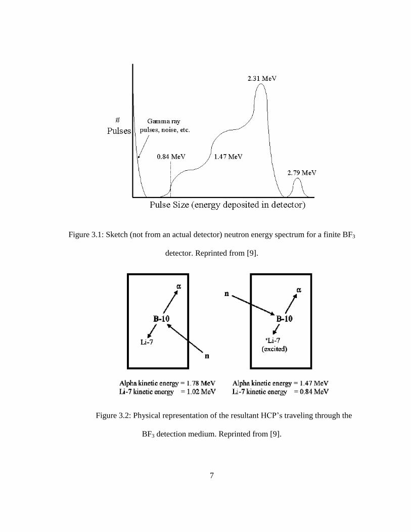
This total energy deposition however is only true if the detector volume is

infinite. While, each of these HCP’s (at these initial kinetic energies) only has a SR of

several cm, that SR may be larger than the distance each particle travels before hitting

the wall of the detector and exiting the detector volume through surface leakage. In this

case, the total energy deposition from each neutron interaction is less than the theoretical

maximum. This is known as the “wall effect”. Why? Well for interactions located closest

to the walls of the detectors the total energy deposition will be the smallest due to the

increased likelihood of surface leakage of a HCP. Figure 3.1 shows that the total energy

deposition for a dummy BF3 does not always match the discrete values of either 2.31

MeV or 2.79 MeV. Additionally, Figure 3.1 shows that the 2.79 MeV total energy

deposition probably is higher than the probability for the 2.31 MeV total energy

deposition reaction. Finally, Figure 3.2 shows a physical representation of the HCP’s

traversing their SR’s in the detection medium. From Figure 3.2 it is obvious to see that it

is possible for the resultant particles to leak out of the detector before depositing all of

their energy.

7

Figure 3.1: Sketch (not from an actual detector) neutron energy spectrum for a finite BF3

detector. Reprinted from [9].

Figure 3.2: Physical representation of the resultant HCP’s traveling through the

BF3 detection medium. Reprinted from [9].

8

While the predominant reaction is defined by Eqs. (3.1) and (3.2) there are also

additional reactions which will be detected by the BF3 which must be accounted for.

Plots of the cross sections of these reactions are shown in Figures 3.3 and 3.4. The data

shown in Figures 3.3 and 3.4 comes from the Evaluated Nuclear Data File (ENDF)

accessed through the Nuclear Energy Agency’s JANIS service [14].

Figure 3.3: Neutron reaction cross sections for 19

F. Reprinted from [14].

Figure 3.4: Neutron reaction cross sections for 10

B. Reprinted from [14].

From Figure 3.3 it is obvious that the predominant way for a neutron/19

F

interaction to result in the production of electrons is the elastic scattering of 19

F which

then subsequently produces a trail of electrons in the gas medium. Additionally, from

9

Figure 3.4 it is obvious that in addition to the reactions described by Eqs. (3.1) and (3.2)

are not the only mechanisms from which electron production can occur due to a

neutron/10

B reaction. It is also possible for the production of a gamma photon and a

recoiling 10

B (of which only the 10

B will interact with the gas and produce electrons).

Finally, another possibility is the production of 11

B which can create its own trail of

electrons as it traverses the gas medium.

As discussed in Section 2, electrons are generated along the path of HCP that is

emitted after the neutron interaction. However, there are still several steps which need to

take place in order to provide an electrical signal to the detector. First, these electrons

must be pulled towards the detector anode wire by an applied electric field described by

Eq. (3.3) [2].

E(r) = V

rln(ba)

. (3.3)

Where E is defined as the electric field, V is the applied voltage, r is the radial distance

from the anode wire, b is the cathode wire inner radius and a is the anode wire outer

radius. The electric field is directly inwards radially from the anode wire. It is assumed

that the initial electrons generated move along the electric field lines coming from the

anode wire.

Gas detectors operate in what is known as the “proportional region”. This means

that the applied voltage is high enough so that when the electrons are being pulled

towards the anode wire, once they are close enough to the anode wire then they will

ionize additional gas molecules. This is due to the electrons being accelerated to a high

10

enough velocity such that they knock loose additional electrons. The resultant electron-

ion pairs move towards the anode wire and knock loose additional electrons. This

cascading process (known as the Townsend avalanche) continues until all electrons

which results from the initial electron are collected on the anode wire. Thus, a

multiplication process has occurred. The total number of electrons collected on the

anode wire resultant from one neutron interaction is a multiplicative factor higher than

the number of electrons initially generated [2]. This allows for a clear electrical signal to

be generated by the detectors and read by the circuits.

3.1 Position Sensitive Detectors

The type of detector described in Section 3 only gives information on the

presence of a neutron. Total neutron counting is a useful tool in that simply determining

the presence of neutrons by seeing if an electrical pulse is generated. Simply detecting

the presence of neutrons is important in areas of non-proliferation. However, this project

seeks to determine not only the presence of thermal neutrons within the detector region

but also the location of their interaction. Thus, modifications to the circuits attached to

the detectors discussed in Section 3 will now be discussed here.

The development of PSD’s began shortly after the general development of

thermal neutron detectors. These detectors can report the position of the neutron

interaction using either a single or multiple anode wires depending on if position

information for a single or for multiple dimensions is desired. The basic principles of

these detectors have remained unchanged since the 1960’s. While there has been some

development in terms of the accuracy of these detectors, an error analysis of the

11

experiment results will be the concern of the experimentalists [3] [4]. Additionally, this

study will only look at 1D detectors as that is the detector currently being used at the

Nuclear Science Center.

The basic principle of getting information about the position of the neutron

interaction is determining the location of the charge centroid correspond to the collection

of electrons on the anode wire. Eq. (3.4) shows how to compute the charge centroid for a

BF3 detector which only has two products which produce electrons:

rQ⃑⃑⃑⃑ =∫ qα(r⃗)r dr + ∫qLi(r⃗)r dr

Qα + QLi. (3.4)

Where rQ⃑⃑⃑⃑ is the position of the charge centroid, qα(r⃗) is the charge per unit length

produced along the path of the alpha particle, qLi(r⃗) is the charge per unit length

produced along the path of the 7Li, Qα is the total charge produced by the alpha particle,

and QLi is the total charge produced by the 7Li ion. The location of this charge centroid

is then projected unto the anode wire. Assuming that the anode wire is straight (a pre-

requisite for Eq. (3.3)) then this projection becomes:

rx⃑⃑⃑⃗ =rQ⃑⃑⃑⃑ ∙ ra⃑⃑⃑⃗

|ra⃑⃑⃑⃗ |2ra⃑⃑⃑⃗ . (3.5)

With rx⃑⃑⃑⃗ as the projection of the charge centroid unto the anode wire and ra⃑⃑⃑⃗ as the vector

going from the start to the end of the anode wire. A 1D thermal neutron detector

obviously only gives a single value for the position of the neutron interaction:

x = |rx⃑⃑⃑⃗ |. (3.6)

Where x is the position readout from the detector. There are two main methods for

determining this position value: charge division and time delay methods.

12

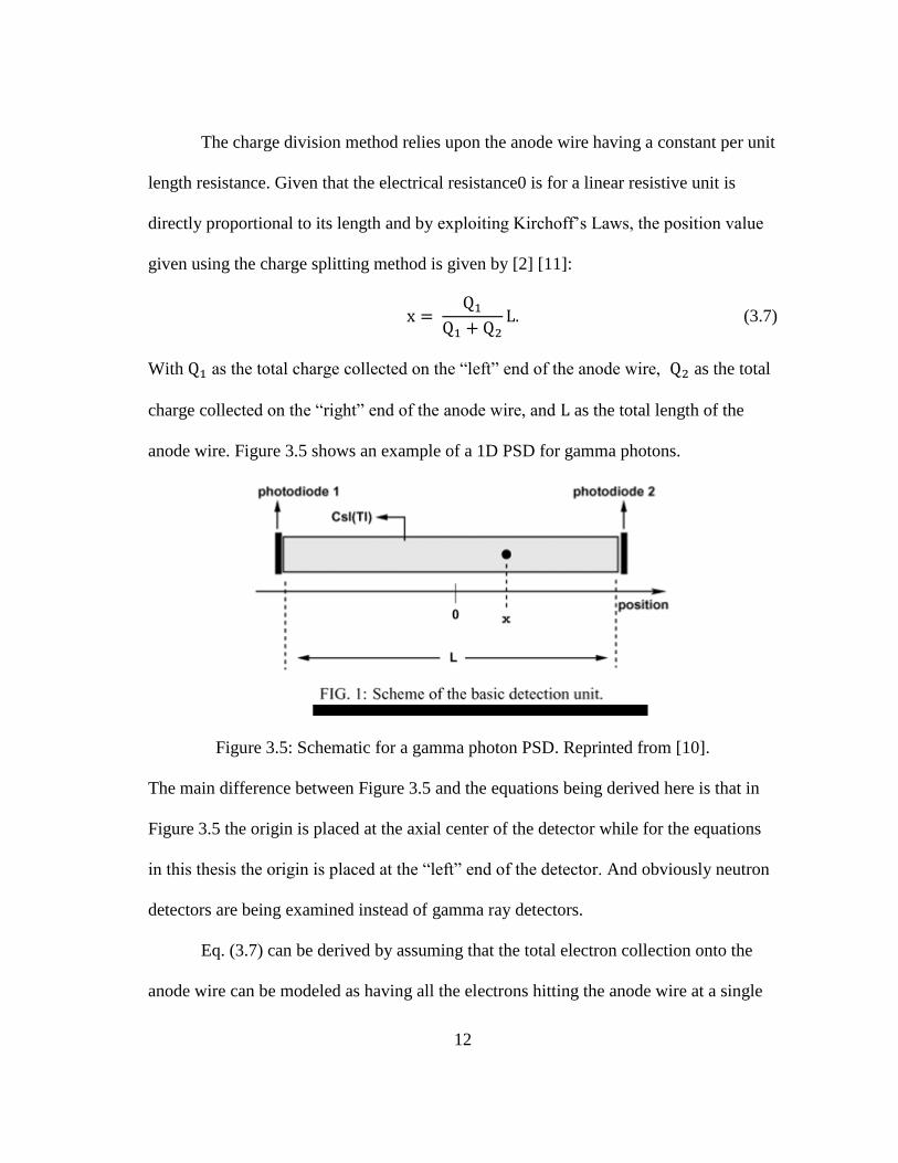
The charge division method relies upon the anode wire having a constant per unit

length resistance. Given that the electrical resistance0 is for a linear resistive unit is

directly proportional to its length and by exploiting Kirchoff’s Laws, the position value

given using the charge splitting method is given by [2] [11]:

x = Q1

Q1 + Q2L. (3.7)

With Q1 as the total charge collected on the “left” end of the anode wire, Q2 as the total

charge collected on the “right” end of the anode wire, and L as the total length of the

anode wire. Figure 3.5 shows an example of a 1D PSD for gamma photons.

Figure 3.5: Schematic for a gamma photon PSD. Reprinted from [10].

The main difference between Figure 3.5 and the equations being derived here is that in

Figure 3.5 the origin is placed at the axial center of the detector while for the equations

in this thesis the origin is placed at the “left” end of the detector. And obviously neutron

detectors are being examined instead of gamma ray detectors.

Eq. (3.7) can be derived by assuming that the total electron collection onto the

anode wire can be modeled as having all the electrons hitting the anode wire at a single

13

point. Thus, the cascade of electrons can be modeled as a current. Thus, the anode wire

can be modeled as a current dividing circuit. Given that the electrical resistance is:

R = ρl

A. (3.8)

where ρ is the material resistivity, l is the resistive element length, and A is the resistive

element cross section area (geometric). The resistance of the left and right sections of the

anode wire relative to x can now be computed as:

R1 = ρx

A. (3.9)

R2 = ρL − x

A. (3.10)

The current-division nature of the circuit also allow for additional equations:

Q = Q1 + Q2. (3.11)

Q1 =R2

R1 + R2Q. (3.12)

Q2 =R1

R1 + R2Q. (3.13)

where Q is the total charge collected. Following algebraic manipulation, Eqs. (3.9)

through (3.13) can be used to show the validity of Eq. (3.7).

The time delay method relies upon the anode wire having both a per unit length

resistance and a per unit length capacitance (an RC transmission wire). By once again

exploiting Kirchoff’s laws, the position of the charge centroid projected onto the anode

wire can be found to be [11]:

14

x =L

2[(t1 − t2)

RC+ 1]. (3.14)

Where L is the total length of the anode wire, t1 is rise the time for the charge to build up

on the “left” side of the detector, t2 is the rise time for the charge to build up on the

“right” side of the detector, R is the total electrical resistance of the anode wire, and C is

the total capacitance of the anode wire. Eq. (3.14) can be derived by first writing down

the resistances and capacitances of each side of the anode wire:

R1 =x

LR. (3.15)

R2 =L − x

LR. (3.16)

C1 =x

LC. (3.17)

C2 =L − x

LC. (3.18)

Additionally, given that each segment of the anode wire is an RC circuit, the rise time

for the charge to build up can be given by:

t1 = R1C1. (3.19)

t2 = R2C2. (3.20)

And thus from Eqs. (3.15) through (3.20) Eq. (3.14) can be found easily through

algebraic manipulation.

Both of the primary methods of getting a reading on the location of the neutron

interaction rely on determining the location of the charge centroid collected on the anode

wire. Because there is only a single anode wire, only a single position value can be

given. So there may be neutron interactions which occur at different locations but who

15

charge centroid gives the same projection unto the anode wire due to having the charge

generation centroid at the same axial position. While MCNP6 can determine the location

of this charge centroid in all three dimensions, the code development will only provide a

single position value along the anode wire to be the output.

3.2 MCNP6: Stochastic Radiation Transport

MCNP6 is considered the gold standard for stochastic radiation transport codes.

The code works by the user defining 1) the problem geometry 2) the materials present in

each part of the problem geometry 3) the source definition and 4) physics and statistics

models to be used for the simulation. The user selects a certain number of particles to be

run. MCNP6 will then simulate each of these particles as they traverse the problem

geometry until some condition is met such as the particle reaching a low enough energy

or the particle exiting the problem geometry. MCNP6 also simulates each of the

secondary radiation which are emitted due to an interaction between the source particle

and the materials present in each section of the problem geometry. The initial properties

of each source and secondary particle are determining through sampling procedures

which make use of random number generators. The interactions each of these particles

undergoes while traversing the problem geometry are also determined through the use of

sampling procedures.

As an example, if a monoenergetic point isotropic source is selected as the source

definition, then for each source particle that is transported MCNP will not sample from

an energy distribution but will sample uniformly from the possible distribution of polar

and azimuthal angles in order to determine the initial direction of the source particles

16

Because only one particle is run at a time, it is necessary to simulate many particles so

that the source actually behaves like a point isotropic source.

MCNP6 contains several specific physics models relating to BF3 detectors and

the transport of the product HCP’s which result from the neutron interaction which need

to be discussed. First, there is only individual tracking for four specific types of heavy

ions (which includes the alpha particle). All of the other species of heavy ions (including

7Li) are tracked together as a group. Thus, some knowledge of the possible reactions

which can occur within the BF3 gas is necessary (for this project it was assumed that all

resultant grouped heavy ions were either 7Li,

10B,

11B, or

19F). Additionally, MCNP6

does not actually track the generation of electrons along the path of the heavy charged

particles. Therefore, the qα(r⃗) and qLi(r⃗) terms in Eq. (3.4) cannot be directly

computed. Therefore, in order to determine the charge centroid in MCNP6 several

assumptions must be made. The material in the detector must be assumed to be

homogeneous and that the HCP’s cause enough ionization such that on average the

number of electrons knocked loose per amount of energy deposited is constant. This

allows for the simplifying assumption to be made:

qα = kdEα

dr⃗. (3.21)

qLi = kdELi

dr⃗. (3.22)

17

Where k is a constant of proportionality defined by the medium the heavy charged

particles are traversing through, Eα is the energy of the alpha particle and ELi is the

energy of the 7Li ion. The total charge terms in Eq. (3.4) can then be re-written as:

Qα = k∫

dEα

dr⃗dr⃗.

(3.23)

QLi = k∫

dELi

dr⃗dr⃗.

(3.24)

Finally, Eq. (3.4) can be re-written as:

rQ⃑⃑⃑⃑ =∫

dEα

dr⃗r dr + ∫

dELi

dr⃗r dr

(Eα,f − Eα,0) + (ELi,f − ELi,0).

(3.25)

Where Eα,f and Eα,0 are the final and initial energies of the alpha particle and ELi,f and

ELi,0 are the final and initial energies of the lithium ion. MCNP6 does offer ways to track

the energies of the alpha particles and 7Li ions; therefore, Eq. (3.25) can be used in

conjunction with Eq. (3.5) in order to determine the predicted position reading.

MCNP6 also has one noticeable deficiency in its physics models in terms of

modeling the resultant products in Eqs. (3.1) and (3.2). The gamma photon in Eq. (3.2)

does not instantaneously decay. Instead the7Li ion will remain in an excited state for a

short time. However, MCNP6 models the 7Li ion as having already ejected the gamma

photon and being at 0.84 MeV. This is not technically correct, although the 7Li ion may

decay so quickly that it does not really matter.

Additionally, MCNP6 does not have options for simulating electric fields.

Therefore, the electric field generated by the anode wire and described by Eq. (3.3)

cannot be inserted into the problem geometry. A code such as GEANT4 would be able

18

to simulate this electric field. In order to get around this, it is assumed that each

generated electron only starts an avalanche at a specific distance from the anode wire.

Thus, the centroid of the charge generation remains the centroid of the charge collection

on the anode wire [2] [5].

Finally, it should be noted that Eq. (3.25) can be re-written to consider the other

possible neutron reactions in the BF3. It is as simple as only including the terms for

energy deposition due to the scattered 10

B, 11

B, or 19

F.

19

4. METHODOLOGY

MCNP6 can compute “tallies” or calculations of various parameters. For

example, MCNP6 can compute the total energy deposition for a given type(s) of

particle(s) in a given cell. This value is then normalized by the mass of the cell (given

the cell’s volume and mass density) and by also normalized by the number of source

particles chosen to be run. The “tally” given from each calculation (as MCNP6 is a

stochastic code) is obviously more accurate given a larger number of source particles

(and therefore greater computational expense).

Vanilla MCNP6 allows for the user to compute a type of calculation which

predicts the response for a position sensitive detector. The position sensitive detector can

be treated by modeling the detector gas volume as multiple cells rather than a single cell.

Next, MCNP6 can compute a F6 energy deposition tally for each of these cells which

compose the position sensitive detector. In the resultant MCNP6 output file, energy

deposition normalized by the mass and number of source particles in each sub-cell of the

position sensitive detector will be given. There are several problems with this method.

First, this method does not track individual neutron interactions, only the total energy

deposition due to secondary radiation resultant of all neutron interactions. Secondly, this

method can be computationally expensive as if a very fine spatial resolution is desired.

Therefore, two main methods will be proposed in order to determine the position

value reported by the detector and also the actual position of the neutron interaction. The

first method will involve exploiting the MCNP6 PTRAC utility. The PTRAC utility

20

allows the user to export a list of particle events (generated from a list of conditions) to

an output file. This PTRAC utility will be used to show that the resultant products from

in Eqs. (3.1) and (3.2) lose energy at a constant rate with respect to their displacement in

the gas volume. This will allow for a simplification to Eq. (3.25) and thus PTRAC will

be used in order to determine both the detector response as well as the actual location of

the neutron interaction.

Additionally, MCNP6 has a user-defined subroutine called TALLYX. Once this

sub-routine is written and the source code is recompiled, modifications to the default

tallies are allowed. At each sub-step of the default tally calculation, TALLYX will also

be called [5]. This allows for TALLYX to use the information at the current sub-step in

order to compute some new value.

4.1 PTRAC

The MCNP PTRAC utility allows for user-selected events to be sent to an output

file. PTRAC will now be used in order to show that energy loss is constant with respect

to displacement for an alpha particle and a 7Li ion with starting energies as shown in

Figure 3.2. An MCNP input file was arranged such that source was either a 1.78 MeV or

1.47 MeV alpha particle moving upwards in the positive Z-direction through a

homogeneous BF3 gas of density 0.00074755 g cm-3

and thickness 10 cm with cell

divisions at every 0.0001 cm in the Z-direction. A total of 10 source particles were run.

The PTRAC files allows for the user to output 1) surface crossing events and 2)

termination events. PTRAC can also list the particle type, position, direction cosines,

energy, time, and particle importance for each event. Thus, this output file can be used in

21

order to extract an E(r⃗) within a specific gas medium for each of the alpha particle and

7Li ion. Figure 4.1 shows an example of a PTRAC file.

Figure 4.1: Example PTRAC file with designated particle events separated into blocks

by source particle number. Reprinted from [7].

From Figure 4.1 it is obvious that PTRAC files are written in such a way that large

amounts of information are present and particle event information is separated by the

source particle corresponding to those particle events. Thus, it should be feasible to write

data processing utilities which can read PTRAC files determine events occurring due to

individual neutron interactions. Figure 4.2 and Figure 4.3 show a reconstruction of E(r⃗)

based upon surface crossing information from the described simulation.

22

Figure 4.2: Energy of a 1.78 MeV alpha particle traversing BF3.

Figure 4.3: Energy of a 1.47 MeV alpha particle traversing BF3.

From Figure 4.2 and Figure 4.3 it is obvious that E(r⃗) is linear over the entire

path of the particle. A regression analysis assuming that E is linear with respect to r⃗ gave

R2 = 0.997262399335 for the case in Figure 4.2 and R

2 = 0.998362384677 for the case

23

in Figure 4.3. This is highly linear relation. Additionally, from Figure 4.2 the stopping

range of the 1.78 MeV alpha particle in this BF3 gas is about 12 mm while for the 1.47

MeV alpha particle the stopping range is reduced to 10 mm.

Additionally, a 1.02 MeV or 0.84 MeV 7Li ion also traversed the same BF3 gas

with a thickness of 2.5 cm and a vertical discretization of 0.00005 cm. The E(r⃗) results

from its surface crossings are shown in Figure 4.4 and Figure 4.5.

Figure 4.4: Energy of a 1.02 MeV lithium ion traversing BF3.

24

Figure 4.5: Energy of a 0.84 MeV lithium ion traversing BF3.

From Figure 4.4 and Figure 4.5 it is obvious that E(r⃗) is linear for these starting

energies of a 7Li ion in BF3. Specifically, a regression analysis assuming that E is linear

with respect to r⃗ gave R2 = 0.999013226294 for Figure 4.4 and R

2 = 0.999094224011

for Figure 4.5. This again represents a highly linear relation for E(r⃗) for these particular

energies and medium for 7Li. Finally, from Figure 4.4 the stopping range of the 1.02

MeV 7Li ion is close to 3 mm while from Figure 4.5 the stopping range of the 0.84 MeV

7Li ion is closer to 2.5 mm.

It should also be noted that the PTRAC file contains the X and Y position data at

each surface crossing. This data indicates (after the PTRAC files were investigated) that

for each of the HCP’s that there was limited movement in the X and Y directions

compared to the total displacement in the Z-direction. This is in agreement with the well-

understood physics of HCP’s traveling in straight lines (outside of massive deflections

due to Rutherford scattering). Finally, it should be noted that the strong linearity in E(r⃗)

25

may actually be unusual since typically there is a strong increase in dE

dr⃗⃑ right before a

charged particle loses all of its energy (Bragg peak) [8].

To further test the assumptions of the physics model, the same set-up was

arranged and test using the Stopping Range of Ions in Matter (SRIM) code. This code

performs a “Ion Distribution and Quick Calculation of Damage” computation as the

HCP traverses the BF3 in order to determine the SR of the particle within the medium.

Note that SRIM considers the boron in the BF3 to be B11

. Figure 4.6 shows 10,000 1.78

MeV alpha particles traveling through BF3, Figure 4.7 shows 10,000 1.47 MeV alpha

particles traveling through BF3, Figure 4.8 shows 10,000 1.02 MeV 7Li ions traveling

through BF3, and finally Figure 4.9 shows 10,000 0.84 MeV 7Li ions traveling through

BF3.

Figure 4.6: Ion damage results with SRIM for 1.78 MeV alpha particles in BF3.

Longitudinal range is 18.0 mm.

26

Figure 4.7: Ion damage results with SRIM for 1.47 MeV alpha particles in BF3.

Longitudinal range is 14.9 mm.

Figure 4.8: Ion damage results with SRIM for 1.02 MeV 7Li ions in BF3. Longitudinal

range is 9.49 mm.

Figure 4.9: Ion damage results with SRIM for 0.84 MeV 7Li ions in BF3. Longitudinal

range is 8.44 mm.

Comparing Figure 4.2 to Figure 4.6, Figure 4.3 to Figure 4.5, Figure 4.4 to

Figure 4.8, and Figure 4.5 to Figure 4.9 it becomes obviously that there is a large

27

discrepancy in the results for the two calculations. MCNP gives a SR for a 1.78 MeV

alpha particle, a 1.47 MeV particle, a 1.02 MeV 7Li ion, and 0.84 MeV

7Li ion

respectively as approximately 12 mm, 9.5 mm, 3 mm, or 2.5 mm respectively. The

SRIM SR results for these respective energies are 18.0 mm. 14.9 mm, 9.49 mm, and

8.44 mm. SRIM predicts for both alpha particles and 7Li ions a much longer stopping

range in the same material given the same initial energy. This could have to do with the

different physics models for lower energy heavy charged particles. At lower energies,

the effect of the electrons of the charged particle becomes more dominant. However,

both SRIM and MCNP6 do predict that the particles generally travel in a straight line.

For the SRIM results there are a handful of large deflections (again see the Rutherford

gold foil experiment) but the particles mostly travel directly to the right with only a

small amount of lateral displacement. Despite the discrepancy in the results, none of the

SRIM numerical results will be used in this analysis as this is an MCNP6 project.

However, this does call into question the integrity of position results obtained using

MCNP6. How MCNP6 transports electrons is heavily documented [5]; however,

transport is for HCP’s is not, leading to the suspicion that perhaps the physics models for

HCP’s are not very robust.

As a final sanity check on the results in Figure 4.2 through Figure 4.9, a direct

computation of the stopping range using the non-relativistic Bethe formula (Eq. (2.2))

and integrating over all possible energies. Eqs. (2.3) through (2.7). First, the mean

excitation energy of boron is 69.7 eV and the mean excitation energy of fluorine is 116.5

eV. The electron density of the boron is 3.360 ∙ 1019

cm-3

and the electron density of the

28

fluorine is 1.814 ∙ 1020

cm-3

. Thus, the total electron density of the BF3 gas is 2.150 ∙ 1020

cm-3

. Further, the mean excitation energy of the BF3 gas is 107.5 eV (0.1075 MeV).

Given that the mass of an electron is 5.488 ∙ 10-4

amu, the mass of an alpha particle is

4.003 amu, and the mass of a 7Li ion is 7.016 amu, a relation for the SR of the

transported ions can be determined for both alpha particles (Eq. (4.1)) and 7LI ions (Eq.

(4.2)):

SR = ∫EdE

8.175 ∙ 1010ln (5.101 ∙ 10−6E). (4.1)

SR = ∫EdE

3.224 ∙ 1011ln (2.911 ∙ 10−6E). (4.2)

Where the units of energy are in eV and the units for stopping range are in mm. Thus,

the stopping range can be computing by integrating Eqs. (4.1) and (4.2) from the starting

particle energy down to the cutoff energy of 1000 eV. Eq. (4.1) gives the SR of a 1.78

MeV alpha particle to be 12.33 mm and the SR of a 1.47 MeV alpha particle to be

particle to be 10.40 mm. Additionally, Eq. (4.2) gives the SR of a 1.02 MeV 7Li ion to

be 2.063 mm and the SR of a 0.84 MeV 7Li ion to be 1.541 mm. These calculations

show much more congruency with the MCNP6 than the SRIM results. This could be due

to the SRIM calculation not being selected to be detailed enough or due to different

physics models used in MCNP6 vs. SRIM calculations. In any case, due to these various

differences in results there is reason to believe that either the MCNP6 models are

incomplete or that during MCNP6 simulations additional physics models needed to be

added to the input file. Table 4.1 summarizes these various results.

29

Table 4.1: SR as predicted from each of the three methods.

SRIM

(mm)

Approximate MCNP

(mm)

Bethe

(mm)

Alpha, 1.78 MeV 18 12 12.33

Alpha, 1.47 MeV 14.9 9.5 10.4

Lithium, 1.02

MeV

9.49 3 2.063

Lithium, 0.84

MeV

8.44 2.5 1.541

One final explanation for the discrepancies between these results is that fluorine

chemical bonding (as take place in BF3) causes large shifts in I. However, SRIM does

not have BF3 available as a material with corrections to the mean excitation energy due

to chemical bonding. Instead, the SRIM simulations were performed assuming that the

BF3 fit into a standard compound model. However this is not the case due to fluorine

chemical bonding [15].

Now that the linearity between the energy and displacement for both 7Li ions and

alpha particles in BF3 gas has been established, Eq (3.25) can be greatly simplified. Eq.

(3.25) can now be re-written. The energy of each of the alpha particle and 7Li ion can

first be written as:

Eα = Es,α +

Et,α − Es,α

|rt,α⃑⃑ ⃑⃑ ⃑ − rs,α⃑⃑ ⃑⃑ ⃑⃑ ||rα⃑⃑ ⃑ − rs,α⃑⃑ ⃑⃑ ⃑⃑ |.

(4.3)

30

ELi = Es,Li +

Et,Li − Es,Li

|rt,Li⃑⃑ ⃑⃑ ⃑⃑ − rs,Li⃑⃑ ⃑⃑ ⃑⃑ ⃑||rLi⃑⃑ ⃑⃑ − rs,Li⃑⃑ ⃑⃑ ⃑⃑ ⃑|.

(4.4)

Where Eα is the energy of the alpha particle, Es,α is the initial energy of the alpha

particle, Et,α is the termination energy of the alpha particle, rα⃑⃑ ⃑ is the position of the alpha

particle, rt,α⃑⃑ ⃑⃑ ⃑ is the final position of the alpha particle, and rs,α⃑⃑ ⃑⃑ ⃑⃑ is the initial position of the

alpha particle. Additionally, ELi is the energy of the 7Li ion, Es,Li is the initial energy of

the7Li ion, Et,Li is the termination energy of the

7Li ion, rLi⃑⃑ ⃑⃑ is the position of the

7Li ion,

rt,Li⃑⃑ ⃑⃑ ⃑⃑ is the final position of the lithium ion, and rs,Li⃑⃑ ⃑⃑ ⃑⃑ ⃑ is the initial position of the lithium

ion. Thus, Eq. (3.12) can be re-written as:

rQ⃑⃑⃑⃑ =

(Es,α − Et,α)(rt,α⃑⃑ ⃑⃑ ⃑ + rs,α⃑⃑ ⃑⃑ ⃑⃑ ) + (Es,Li − Et,Li)(rt,Li⃑⃑ ⃑⃑ ⃑⃑ + rs,Li⃑⃑ ⃑⃑ ⃑⃑ ⃑)

2[(Es,α − Et,α) + (Es,Li − Et,Li)].

(4.5)

Eq. (4.5) can only be used by appropriately setting up the MCNP6 input file.

First, Eq. (4.5) assumes that the only HCP’s which are generated within the detector gas

volume come from neutron interactions within the gas. While this will be mostly true it

is not impossible for secondary radiation to penetrate the detector wall from the outside

and deposit energy into the detector volume. However, this is not typically what happens

and therefore the simplification can be made that the only HCP’s that are of concern

come from interactions within the detector gas volume. This simplification is also

important as by not simulating the production or transport of HCP’s in other parts of the

problem geometry, computational expense is greatly lowered. Additionally, Eq. (4.5)

assumes that a neutron interaction necessarily results in the production of an alpha

particle and 7Li ion every time. However, this is not true-as stated before elastic

31

scattering events can occur in which case only the term for the heavy ion (7Li,

10B,

11B,

or 19

F) will be taken into account. Finally, reading from the PTRAC file can give both

the results of the detector response as well as the actual location of the neutron

interaction. Having both of these results allows for a comparison of the neutron

distribution in order to observe a wall effect.

In order to properly generate the PTRAC file, several steps must be taken. First,

the user must define an F6 (total energy deposition) tally for the gas volume cell which

includes both alpha particles and generic heavy ions. Next, the user must ask for all the

PTRAC output to be all particle events which contribute to the F6 tally. Thus, the

PTRAC file will include both birth and termination events for all product heavy ions and

alpha particles. An alternate way to perform would be to not specify a tally with PTRAC

and instead directly call for birth and termination events of alpha particles and heavy

ions. Because alpha particles and heavy ions are killed once leaving the gas volume,

termination events correspond to both surface leakage of HCP’s as well termination due

to the particle energy being too low.

PTRAC files are difficult to interpret from their explanation given in the MCNP6

user manual. A simpler explanation follows. Each block within the PTRAC output file

represents all the particle events which correspond to a source particle. The number of

the source particle is given in each block. Additionally, for each particle the type of

event (looking for birth or termination), type of particle, and particle position, direction,

energy, weight, and time are given. All of this information allows for a computation of

the electron generation centroid.

32

The type of reaction which occurs is determined from the particle weight. To

greater simply matters, MCNP6 treats each generated particle differently. Effectively

each particle that is transported in MCNP6 is only actually some fraction (weight) of a

particle. HCP’s have a constant weight as they traverse a medium. Thus, all particle

events within a source particle data block where the weight is the same correspond to a

single reaction, either an alpha particle-7Li ion pair or an elastic scatter. Thus, when the

position projection from Eqs. (3.5) and (3.6) for either the neutron interaction or detector

response is calculated the value entered into the histogram bin is the weight for the

particles in the reaction. This is the correct way of performing this calculation as

MCNP6 performs a similar method when computing surface fluxes [5].

4.2 TALLYX

MCNP6 contains a blank subroutine file (TALLYX) which the user is allowed to

modify in order to compute custom tallies. The custom tallies are based upon the default

tallies. If some tally Fn is asked to be calculated then this tally can be modified with the

FUn tally. TALLYX is only called if FUn is present in the MCNP6 input file. TALLYX

is written in FORTRAN90 and after the subroutine is written the entire MCNP6

executable must be re-compiled. The author of this thesis compiled the new build on

Ubuntu 16.04 using the gfortran 5.4 and gcc 5.4 compilers [5] [6].

TALLYX is called for each substep of the tally computation. If a tally considers

certain types of particles then each substep contains information on the particle type,

position, and energy. Therefore, it is obvious how TALLYX can be used in order to

33

determine position information as information on particle energy and position as each

particle in a tally traverses a cell is available.

The main method is to insert a F6:A,# energy deposition calculation into the

input file. This method will be largely similar to the PTRAC method discussed in

Section 4.1. Essentially, each time TALLYX is called information about the current

substep of the calculation (particle type, position, energy, current source particle count)

is written to an output file. In a way, this is similar to how a PTRAC file can contain

information regarding these same properties but only for the birth and termination points

for each particle. However, this method should provide the largest accuracy because as

seen in Section 4.1 and Figures 4.5 through 4.9 that assuming that these HCP’s travel in

entirely straight lines is not entirely appropriate. And even if the paths are on average

straight, the distance traveled is greater than a direct path from starting point to end

point. Additionally, linearity was not established for the additional elastic scatter

reactions or for alternate materials or gas densities. While the written output file does not

contain all information regarding the path of each heavy charged particle, the

discretization is very fine-some of the test problems showed that about 104-10

5 events

were written while tracing each HCP. Thus, a modified form of Eq. (4.5) is required in

order to properly mine this new PTRAC-like file:

rQ⃑⃑⃑⃑ =

∑ [(Es,α − Et,α)(rt,α⃑⃑ ⃑⃑ ⃑ + rs,α⃑⃑ ⃑⃑ ⃑⃑ )]n

∞n=1 + ∑ [(Es,Li − Et,Li)(rt,Li⃑⃑ ⃑⃑ ⃑⃑ + rs,Li⃑⃑ ⃑⃑ ⃑⃑ ⃑)]m

∞m=1

∑ [2(Es,α − Et,α)]n∞n=1 + ∑ [2(Es,Li − Et,Li)]m

∞m=1

. (4.6)

Eq. (4.6) is nearly similar to Eq. (4.5) with one noticeable difference. Instead of

assuming constant energy loss over the entirely length of the particle trajectory, instead

34

energy loss is assumed to be constant (constant stopping power) between each of the

many substeps for each particle. The subscripts “n” and “m” refer to the substeps of the

alpha particle and 7Li ion respectively. Obviously, as with previous methods discussed

Eq. (4.6) can also be used just in the case of the solo production of a HCP from elastic

scatter. Similar to the PTRAC method, the output file is mined for the necessary

information. For each source particle, all energy deposition from HCP’s traversing the

cell is considered. A position is then calculated and binned using Eq. (3.5).

This method holds the most promise and follows the greatest rigor. However, one

severe limitation is that the output files generated can be quite large (in excess of 1 GB).

While there may be a limitation in terms of disc space, Python is perfectly capable of

reading these large files in a matter of 5-10 minutes per 1 GB of text file data. Still, a

way to store this data in memory would be useful for rigor and also preventing

overfilling the local drive. A likely method would be to avoid writing this large file to

begin with and create additional global variables within the MCNP6 source code.

However, this was found to require extensively modifying the MCNP6 source code.

Such an undertaking would be beyond the scope of this project and it would reduce the

ability for other users to implement the methods developed in this project.

35

5. TEST PROBLEMS AND RESULTS

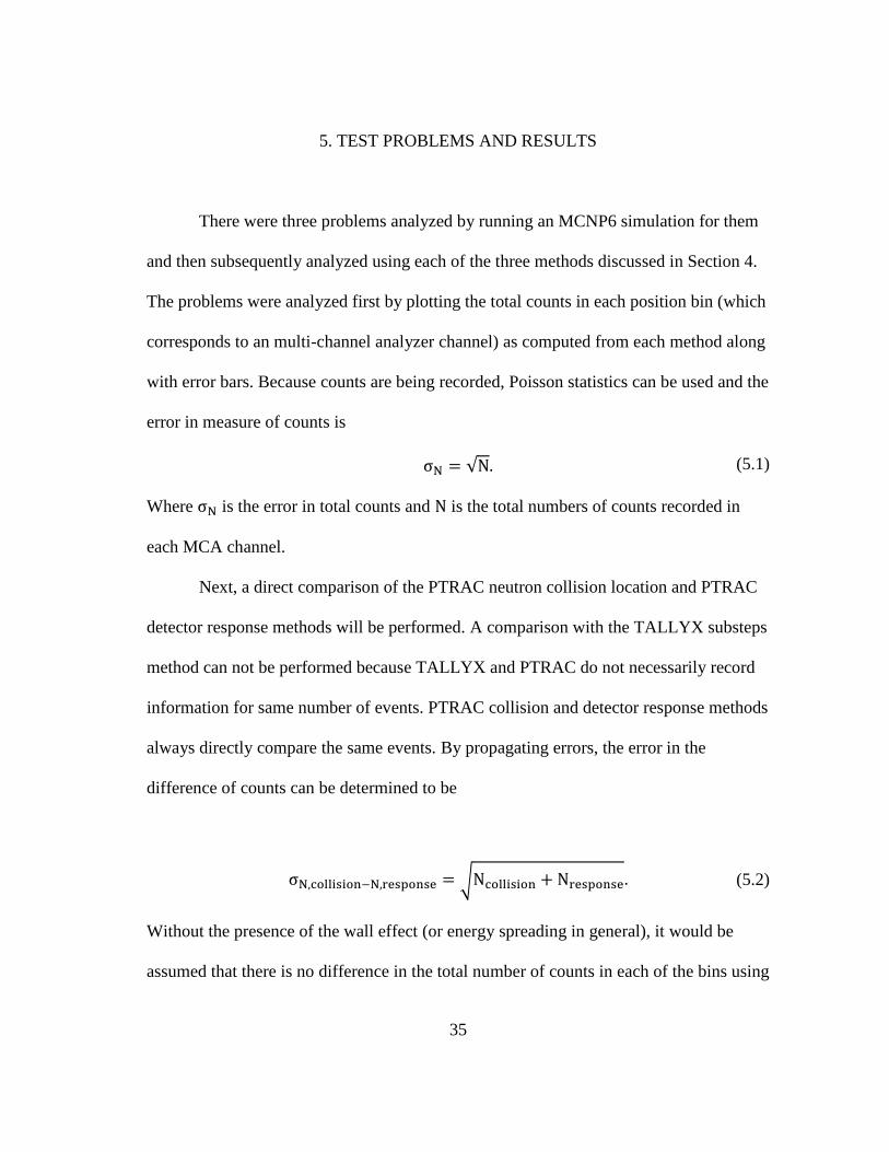
There were three problems analyzed by running an MCNP6 simulation for them

and then subsequently analyzed using each of the three methods discussed in Section 4.

The problems were analyzed first by plotting the total counts in each position bin (which

corresponds to an multi-channel analyzer channel) as computed from each method along

with error bars. Because counts are being recorded, Poisson statistics can be used and the

error in measure of counts is

σN = √N. (5.1)

Where σN is the error in total counts and N is the total numbers of counts recorded in

each MCA channel.

Next, a direct comparison of the PTRAC neutron collision location and PTRAC

detector response methods will be performed. A comparison with the TALLYX substeps

method can not be performed because TALLYX and PTRAC do not necessarily record

information for same number of events. PTRAC collision and detector response methods

always directly compare the same events. By propagating errors, the error in the

difference of counts can be determined to be

σN,collision−N,response = √Ncollision + Nresponse. (5.2)

Without the presence of the wall effect (or energy spreading in general), it would be

assumed that there is no difference in the total number of counts in each of the bins using

36

either the PTRAC collision or detector response methods. However, obviously energy

spreading does occur. A chi-squared test can show exactly to what degree these two

methods differ. The chi-squared statistic can be computed from

χ2 = ∑(Ncollision − Ndetector

σN,collision−N,detector)2

∞

i=1

. (5.3)

A reduced chi-squared can be determined from

χν2 =

χ2

ν. (5.4)

Where ν is the number of degrees of freedom. The number of degrees of freedom can be

determined from

ν = n − f. (5.5)

Where n is the number of position bins (MCA channels) and f is the number of fitting

parameters. For this first analysis (difference in results between the PTRAC collision

and detector response results) there are no fitting parameters. A lower value for χν2

indicates a better fit. Typically, a value less than 1 is considered the most desirable

result.

Finally, a regression analysis for each of the test problems will be performed by

first proposing a theoretical model for the detector response using the TALLYX substeps

method. The theoretical model will include fitting parameters. Finding the optimal

values for these parameters will consist of a simple Excel procedure involving the

minimization of the reduced chi-squared value from Eq. (5.4).

37

5.1 Line Detector

The first problem run had a monoenergetic (thermal) 2.5 ∙ 10-8

MeV neutron

source. This source was placed directly below the center of an 80 cm long (with a radius

of 2.5 cm) BF3 tube (gas only, no shell). The distance from the source to the tube was 40

cm and the rest of the problem was a vacuum. The source only emitted neutrons in the

plane defined by a line running along the central axis of the gas volume and by a line

going from the source to the centroid of the detector. A total of 108 source neutrons were

simulated. The count data was sorted into 25 position bins. Figure 5.1 shows the position

binning (with error bars) with all three methods while Figure 5.2 shows the difference

between the two PTRAC methods.

Figure 5.1: Counts and counting error results for all three methods (line detector).

0

2000

4000

6000

8000

10000

12000

14000

16000

18000

0 10 20 30

Counts

Position Bin

Line Detector

PTRAC Collision

PTRAC Response

TALLYX

Response

38

Figure 5.2: Counts difference between the two PTRAC methods (line detector).

From Figure 5.1 it is obvious that the PTRAC results match each very closely while the

TALLYX results oddly reports a low total count of detected interactions. However, this

is somewhat to be expected as these methods give different consideration when reporting

pertinent events. A reduced chi-squared value for the data in Figure 5.2 gives a result of

0.126079608 indicating that the predicted detector response and the actual location of a

neutron interaction are very close-there is only a minimal wall effect.

Because this is a line detector (the gas medium is assumed to be thin) an

analytical expression exists for the position spectrum.

C =P

s2 + 1600. (5.6)

Where C is the number of counts in the bin, P is some fitting parameter and should be

equal to the counts in the central position, and s is the distance (in cm) from the center of

-300

-200

-100

0

100

200

300

0 5 10 15 20 25 30

Counts

Dif

fere

nce

Position Bin

Line Detector

39

a bin to the center of the central bin. Figure 5.3 shows a plot of the TALLYX results

along with the fitted curve which resulted from chi-squared minimization.

Figure 5.3: TALLYX curve fitting results (line detector).

The results from Figure 5.3 gave a result for the fitting parameter P to be

24504778.17 reduced chi-squared value of 9.814650108 which indicates a poor fit to the

data as this is far greater than 1. Possible reasons for this include the fact that TALLYX

records far fewer events than PTRAC for this problem, especially at the outermost

position bins as seen in Figure 5.1. Additionally, the analytical solution from Eq. (5.6) is

perhaps wrong. The detector is not exactly a line detector-it has some thickness and

neutrons arriving in the outermost position bins actually travel through a larger thickness

of the material, causing a higher number of interactions in those regions. The drop-off

would be expected to be ½ moving from the central to outermost bins; however, the

drop-off is much less than this.

0

2000

4000

6000

8000

10000

12000

14000

16000

18000

0 10 20 30

Counts

Position Bin

Line Detector

TALLYX

Response

Fitted Curve

40

5.2 Modified Localized Source Experiment

Another experiment analyzed was a localized source experiment. Figure 5.4

shows the arrangement for the detector tube but not the source used in this experiment.

Figure 5.4: BF3 gas detector (much lower density than the simulations in Section 4.1)

wrapped with an aluminum shell and wrapped in cadmium with a slit in the central

portion of the tube. Reprinted from [16].

Not shown in Figure 5.4 is the fact that the neutron source was an AmBe mixed-field

source wrapping in a moderating high density polyethylene material. This source-

moderator component was placed directly over the opening in the cadmium wrapping.

The total length of the aluminum tube was 91.44 cm and the opening in the slit was

0.3175 cm. While the neutron interactions would be expected to mostly concentrated

within the area of the slit they would also appear in position bins outside of this region as

well because the beam of neutrons entering the slit is not a collimated beam. However,

because the slit is so far from the outermost bins, no large wall effect should be present.

The remainder of the problem outside of what was described above is treated as vacuum.

The count data was sorted into 288 position bins. Figure 5.5 shows the position binning

41

(with error bars) with all three methods while Figure 5.6 shows the difference between

the two PTRAC methods.

Figure 5.5: Counts and counting error results for all three methods (localized source).

-500

0

500

1000

1500

2000

2500

3000

3500

0 100 200 300 400

Counts

Position Bin

Localized Source

PTRAC Collision

PTRAC Response

TALLYX

Response

42

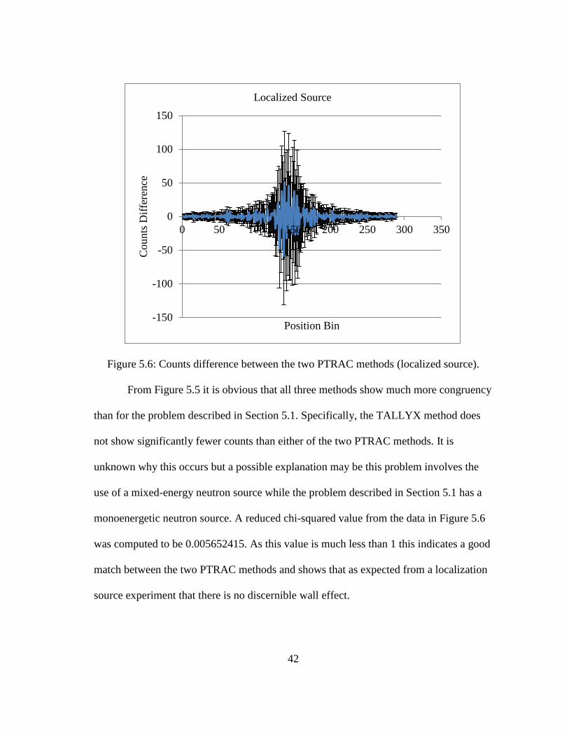
Figure 5.6: Counts difference between the two PTRAC methods (localized source).

From Figure 5.5 it is obvious that all three methods show much more congruency

than for the problem described in Section 5.1. Specifically, the TALLYX method does

not show significantly fewer counts than either of the two PTRAC methods. It is

unknown why this occurs but a possible explanation may be this problem involves the

use of a mixed-energy neutron source while the problem described in Section 5.1 has a

monoenergetic neutron source. A reduced chi-squared value from the data in Figure 5.6

was computed to be 0.005652415. As this value is much less than 1 this indicates a good

match between the two PTRAC methods and shows that as expected from a localization

source experiment that there is no discernible wall effect.

-150

-100

-50

0

50

100

150

0 50 100 150 200 250 300 350

Counts

Dif

fere

nce

Position Bin

Localized Source

43

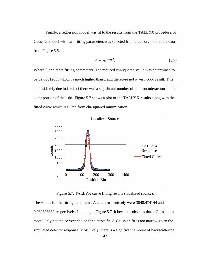
Finally, a regression model was fit to the results from the TALLYX procedure. A

Gaussian model with two fitting parameters was selected from a cursory look at the data

from Figure 5.5.

C = Ae−αs2. (5.7)

Where A and α are fitting parameters. The reduced chi-squared value was determined to

be 32.86812053 which is much higher than 1 and therefore not a very good result. This

is most likely due to the fact there was a significant number of neutron interactions in the

outer portion of the tube. Figure 5.7 shows a plot of the TALLYX results along with the

fitted curve which resulted from chi-squared minimization.

Figure 5.7: TALLYX curve fitting results (localized source).

The values for the fitting parameters A and α respectively were 3048.474144 and

0.032898382 respectively. Looking at Figure 5.7, it becomes obvious that a Gaussian is

most likely not the correct choice for a curve fit. A Gaussian fit is too narrow given the

simulated detector response. Most likely, there is a significant amount of backscattering

-500

0

500

1000

1500

2000

2500

3000

3500

0 100 200 300 400

Counts

Position Bin

Localized Source

TALLYX

Response

Fitted Curve

44

of neutrons within the detector tube which is leading neutron interactions outside of the

area local to the source.

5.3 Modified Impurity Model (IM-1) Experiment

IM-1 was a series of experiments of high complexity which can not be accurately

described here in words. These experiments involved using an AmBe mixed-field

neutron source which then traversed through a large number of moderating materials in

order to reach a spherical BF3 detector which actually has the same gas density as the

simulations from Section 4.1. An example of an IM-1 experiment (which was not

actually the one simulated for this thesis) is shown in Figure 5.8.

Figure 5.8: A representative example of an IM-1 experiment. Reprinted from [13].

45

The particular experiment in Figure 5.8 was analyzed in a large amount of detail

by a previous graduate student. Figure 5.8 also provides a nice visualization how the

spherical detector is covered by the boral shroud. In the experiment, the BF3 detector

was not position sensitive however for the purpose of the simulations it was assumed

that the anode wire ran along the y-axis (referencing Figure 5.8) and through the center

of the sphere. The count data was sorted into 5 position bins. Figure 5.9 shows the

position binning (with error bars) with all three methods while Figure 5.10 shows the

difference between the two PTRAC methods.

Figure 5.9: Counts and counting error results for all three methods (IM-1).

0

10

20

30

40

50

60

0 2 4 6

Counts

Position Bin

IM-1

PTRAC Collision

PTRAC Response

TALLYX

Response

46

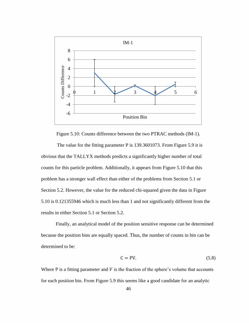
Figure 5.10: Counts difference between the two PTRAC methods (IM-1).

The value for the fitting parameter P is 139.3601073. From Figure 5.9 it is

obvious that the TALLYX methods predicts a significantly higher number of total

counts for this particle problem. Additionally, it appears from Figure 5.10 that this

problem has a stronger wall effect than either of the problems from Section 5.1 or

Section 5.2. However, the value for the reduced chi-squared given the data in Figure

5.10 is 0.121355946 which is much less than 1 and not significantly different from the

results in either Section 5.1 or Section 5.2.

Finally, an analytical model of the position sensitive response can be determined

because the position bins are equally spaced. Thus, the number of counts in bin can be

determined to be:

C = PV. (5.8)

Where P is a fitting parameter and 𝑉 is the fraction of the sphere’s volume that accounts

for each position bin. From Figure 5.9 this seems like a good candidate for an analytic

-6

-4

-2

0

2

4

6

8

0 1 2 3 4 5 6

Co

un

ts D

iffe

ren

ce

Position Bin

IM-1

47

solution-the position bins in the outer regions have far fewer counts. Figure 5.11 shows a

plot of the TALLYX results along with the fitted curve which resulted from chi-squared

minimization.

Figure 5.11: TALLYX curve fitting results (IM-1).

The chi-squared minimization results in a reduced chi-squared value of

2.072066681. This indicates a poor fit. However, given the asymmetry of the TALLYX

result as seen in Figure 5.11 it is possible that this is due to simply not having enough

total counts recorded. However, given the complexity of the problem as seen in the

representative sample in Figure 5.8 this would be unwieldy and result in a simulation

with perhaps too large of a computational expense. However, this was also the lowest

reduced chi-squared of all analytical models proposed in either Section 5.1, Section 5.2,

or Section 5.3. It is probably correct however the counts are too low. It should also be

noted that Eq. (5.1) was used when computing all of the various errors; however, in

some cases perhaps the number of counts was too low in order to apply Eq. (5.1).

0

10

20

30

40

50

60

0 2 4 6

Co

un

ts

Position Bin

IM-1

TALLYX Response

Curve Fit

48

6. CONCLUSIONS

Multiple methods were developed using the MCNP6 code in order to provide

predictions for a the response of a 1D neutron PSD. However, there is some concern as

to whether or not MCNP6 correctly models HCP’s as well as it models electrons.

Additionally, the PTRAC methods were consistent across all three of the test problems

in that only a minimal wall effect was observed. This was surprising as the SR of alpha

particles and 7Li ions was found to be larger than the position bin size in some of these

problems. Additionally, it was found that PTRAC and TALLYX did not even record the

same events. There appears to be several possible reasons for this; however, due to the

hidden nature of MCNP6’s inner-workings it is not within the scope of this thesis to try

and discover the reason for this discrepancy. Finally, none of the theoretical models

matched any of the TALLYX results from each problem. This may been due to

insufficient detail (backscattering of neutrons) or not enough counts or possible in the

case of the problem described in Section 5.1 a TALLYX modification to a surface flux

tally would have proved much more useful.

49

REFERENCES

[1] Crane, T.W., and M.P. Baker. “Neutron Detectors.” Passive Nondestructive Assay

Manual. Los Alamos National Laboratory.

http://www.lanl.gov/orgs/n/n1/panda/00326408.pdf

[2] Knoll, G.F. Radiation Detection and Measurement. 4th ed. New York: Wiley, 2010.

[3] Crawford, R.K. “Position-sensitive detection of slow neutrons-survey of

fundamental principles.” Office of Scientific and Technical Information. 1992.

https://www.osti.gov/scitech/servlets/purl/5095599-6rb0Q6/

[4] Convert, P. and J.B. Forsyth. “The Principles of Thermal Neutron Production,” and

“An Introduction to the Types of Position-sensitive Neutron Detectors.” Position-

Sensitive Detection of Thermal Neutrons. Eds. Convert, P. and J.B. Forsyth. New

York: Academic Press, 1983. 1-46.

[5] D.B. Pelowitz, Ed., "MCNP6 Users Manual Version 1.0" LA-CP-13-00634 (2013).

[6] Solomon, C.J. “A Patch to MCNP5 for Multiplication Interference: Description and

User Guide” LA-UR-14-23160 (2011).

[7] Stevenson, A.W. Improving the Efficiency of Photon Collection By Compton

Rescue. MS Thesis, Air Force Institute of Technology, 2011.

http://www.dtic.mil/dtic/tr/fulltext/u2/a538792.pdf

[8] Turner, J.E. Atoms, Radiation, and Radiation Protection. 3rd edition. Wiley-VCH:

Weinheim, 2008. 109-137.

[9] Frame, P. “Boron Trifluoride (BF3) Neutron Detectors.” Oak Ridge Associated

50

Universities. 1999.

https://www.orau.org/ptp/collection/proportional%20counters/bf3info.htm

[10] de Almeida, M. and M. Moralles. “Monte Carlo simulation of a position sensitive

gamma ray detector.” Brazilian Journal of Physics, 2005.

http://www.scielo.br/pdf/bjp/v35n3b/a04v353b.pdf

[11] Spieler, H. “Position-Sensitive Detectors.” University of California, Berkeley,

1998. http://www-physics.lbl.gov/~spieler/physics_198_notes/PDF/VI-PSD.pdf

[12] Tesinsky, M. “MCNPX Simulations for Neutron Cross Section Measurements.”

MS Thesis, Royal Institute of Technology, 2010.

ftp://ftp.nrg.eu/pub/www/talys/tendl2010/presentations/TesinskyMilan.pdf

[13] Ghaddar, T. Load Balancing Unstructured Meshes For Massively Parallel

Transport Sweeps. MS Thesis, Texas A&M University, 2016.

http://oaktrust.library.tamu.edu/bitstream/handle/1969.1/157129/GHADDAR-

THESIS-2016.pdf?sequence=1&isAllowed=y

[14] M.B. Chadwick, M. Herman, P. Obložinský, M.E. Dunn, Y. Danon, A.C. Kahler,

D.L. Smith, B. Pritychenko, G. Arbanas, R. Arcilla, R. Brewer, D.A. Brown, R.

Capote, A.D. Carlson, Y.S. Cho, H. Derrien, K. Guber, G.M. Hale, S. Hoblit, S.

Holloway, T.D. Johnson, T. Kawano, B.C. Kiedrowski, H. Kim, S. Kunieda,

N.M. Larson, L. Leal, J.P. Lestone, R.C. Little, E.A. McCutchan, R.E.

MacFarlane, M. MacInnes, C.M. Mattoon, R.D. McKnight, S.F. Mughabghab,

G.P.A. Nobre, G. Palmiotti, A. Palumbo, M.T. Pigni, V.G. Pronyaev, R.O. Sayer,

A.A. Sonzogni, N.C. Summers, P. Talou, I.J. Thompson, A. Trkov, R.L. Vogt,

51

S.C. van der Marck, A. Wallner, M.C. White, D. Wiarda, P.G. Young,

"ENDF/B-VII.1: Nuclear Data for Science and Technology: Cross Sections,

Covariances, Fission Product Yields and Decay Data", Nucl. Data Sheets

112(2011)2887.

[15] Ziegler, J.F., and Manoyan, J.M. “The Stopping of Ions in Compounds.” Nuclear

Instruments and Methods in Physics Research B35, 1988, 215-228.

http://www.sciencedirect.com/science/article/pii/0168583X8890273X

[16] Pongpun, Sophit. “BF3 Cylindrical Tube Preliminary Test Results

Data Acquisition Date: May 19, 2017.” Internal report. 13 June 2017.