McGraw-Hill 10-1. 10 McGraw-Hill Systems Analysis & Programming.
Upload
dominic-ordwayCategory
view
213download
0
© The McGraw-Hill Companies, Inc., 200819.1McGraw-Hill/Irwin
Table of ContentsCD Chapter 19 (Inventory Management with Uncertain Demand)
A Case Study for Perishable Products—Freddie the Newsboy (Section 19.1) 19.2–19.3
An Inventory Model for Perishable Products (Sec.19.2) 19.4–19.12
A Case Study for Stable Products—Niko Camera Corp. (Section 19.3) 19.13–19.18
The Management Science Team’s Analysis of the Case Study (Section 19.4) 19.19–19.32
A Continuous-Review Inventory Model for Stable Products (Section 19.5) 19.33–19.42
Larger Inventory Systems in Practice (Section 19.6) 19.43
© The McGraw-Hill Companies, Inc., 200819.2McGraw-Hill/Irwin
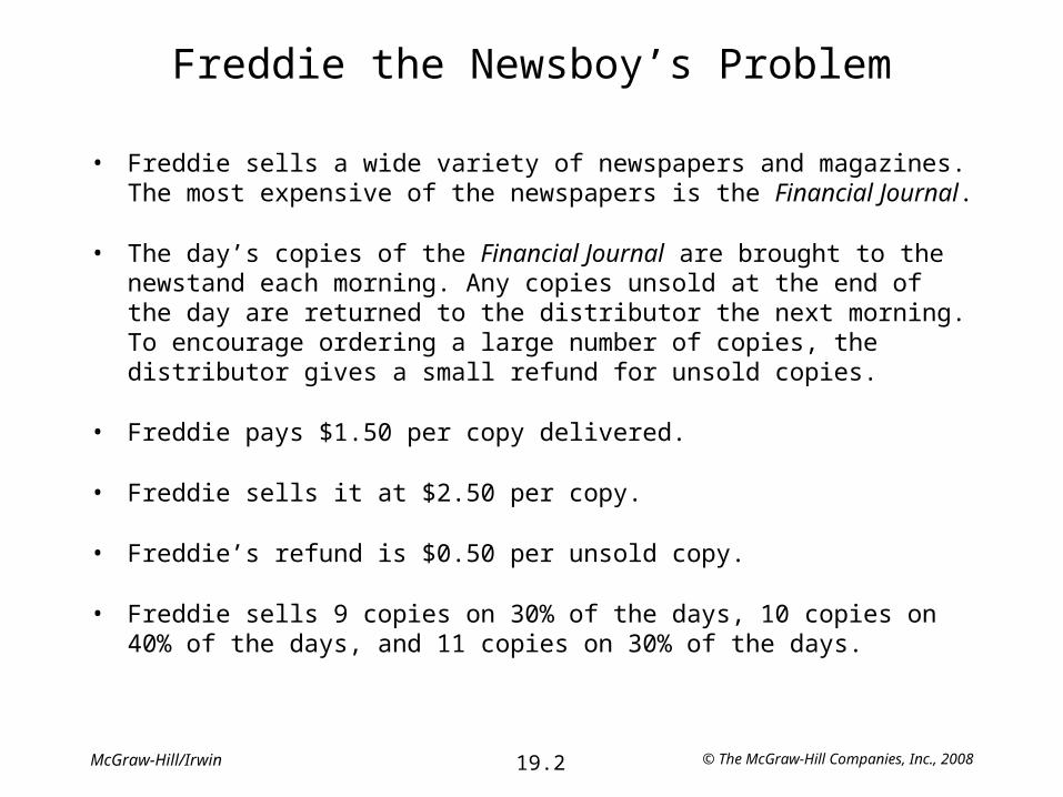
Freddie the Newsboy’s Problem
• Freddie sells a wide variety of newspapers and magazines. The most expensive of the newspapers is the Financial Journal.
• The day’s copies of the Financial Journal are brought to the newstand each morning. Any copies unsold at the end of the day are returned to the distributor the next morning. To encourage ordering a large number of copies, the distributor gives a small refund for unsold copies.
• Freddie pays $1.50 per copy delivered.
• Freddie sells it at $2.50 per copy.
• Freddie’s refund is $0.50 per unsold copy.
• Freddie sells 9 copies on 30% of the days, 10 copies on 40% of the days, and 11 copies on 30% of the days.
© The McGraw-Hill Companies, Inc., 200819.3McGraw-Hill/Irwin
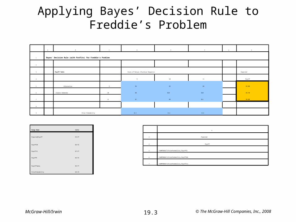
Applying Bayes’ Decision Rule to Freddie’s Problem
Range Name Cells
ExpectedPayoff H5:H7
Payoff10 D6:F6
Payoff11 D7:F7
Payoff9 D5:F5
PayoffTable D5:F7
PriorProbability D9:F9
1
2
3
4
5
6
7
8
9
A B C D E F G H
Bayes' Decision Rule (with Profits) for Freddie's Problem
Payoff Table State of Nature (Purchase Requests) Expected
9 10 11 Payoff
Alternative 9 $9 $9 $9 $9.00
(Copies Ordered) 10 $8 $10 $10 $9.40
11 $7 $9 $11 $9.00
Prior Probability 0.3 0.4 0.3
3
4
5
6
7
H
Expected
Payoff
=SUMPRODUCT(PriorProbability,Payoff9)
=SUMPRODUCT(PriorProbability,Payoff10)
=SUMPRODUCT(PriorProbability,Payoff11)

© The McGraw-Hill Companies, Inc., 200819.4McGraw-Hill/Irwin
Assumptions for an Inventory Model for Perishable Products
• Each application involves a single perishable product.
• Each application involves a single time period because the product can’t be sold later.
• However, it will be possible to dispose of any units remaining at the end of the period, perhaps receiving a salvage value for the units.
• The only decision to be made is how many units to order (the order quantity).
• The demand during the period is uncertain. However, the probability distribution of demand is known (or at least estimated).
• If the demand exceeds the order quantity, a cost of underordering is incurred. In particular, cunder = decrease in profit from failing to order a unit that could have been sold during the period.
• If the order quantity exceeds the demand, a cost of overordering is incurred. In particular, cover = decrease in profit from ordering a unit that could not be sold during the period.

© The McGraw-Hill Companies, Inc., 200819.5McGraw-Hill/Irwin
Applying Bayes’ Decision Rule to Freddie’s Problem
1
2
3
4
5
6
7
8
9
A B C D E F G H
Bayes' Decision Rule (with Costs) for Freddie's Problem
Payoff Table State of Nature (Purchase Requests) Expected
9 10 11 Payoff
Alternative 9 $0 $1 $2 $1.00
(Copies Ordered) 10 $1 $0 $1 $0.60
11 $2 $1 $0 $1.00
Prior Probability 0.3 0.4 0.3

© The McGraw-Hill Companies, Inc., 200819.6McGraw-Hill/Irwin
Ordering Rule for the Model for Perishable Products
• Optimal service level
• Choose the smallest order quantity that provides at least this service level.
=cunder
cunder + cover

© The McGraw-Hill Companies, Inc., 200819.7McGraw-Hill/Irwin
Applying the Ordering Rule to Freddie’s Problem
cunder = unit sales price – unit purchase cost = $2.50 – $1.50 = $1.00
cover = unit purchase cost – unit salvage value = $1.50 – $0.50 = $1.00
Optimal Service Level
Service Level if order 9 copies = 0.3Service level if order 10 copies = 0.3 + 0.4 = 0.7Service level if order 11 copies = 0.3 + 0.4 + 0.3 = 1.0
The smallest order quantity that provides at least the optimal service level is to order 10 copies.
=$1.00
$1.00 + $1.00= 0.5

© The McGraw-Hill Companies, Inc., 200819.8McGraw-Hill/Irwin
Excel Template for Perishable Products
1
2
3
4
5
6
A B C D E F
Optimal Service Level for Perishable Products
Data Results
Unit Sales Price $2.50 Cost of Overordering $1.00
Unit Purchase Cost $1.50 Cost of Underordering $1.00
Unit Salvage Value $0.50 Optimal Service Level 0.5
4
5
6
E F
Cost of Overordering =UnitPurchaseCost-UnitSalvageValue
Cost of Underordering =UnitSalesPrice-UnitPurchaseCost
Optimal Service Level =CostOfUnderordering/(CostOfUnderordering+CostOfOverordering)
Range Name Cell
CostOfOverordering F4
CostOfUnderordering F5
OptimalServiceLevel F6
UnitPurchaseCost C5
UnitSalesPrice C4
UnitSalvageValue C6

© The McGraw-Hill Companies, Inc., 200819.9McGraw-Hill/Irwin
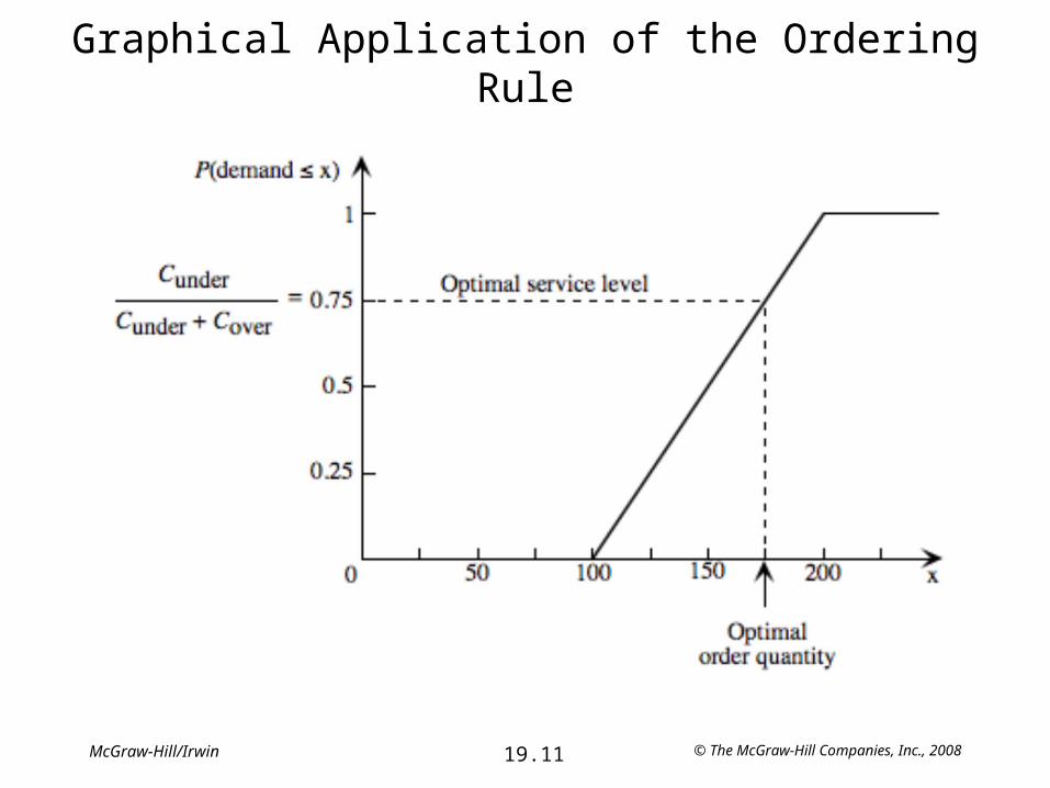
Graphical Application of the Ordering Rule
© The McGraw-Hill Companies, Inc., 200819.10McGraw-Hill/Irwin
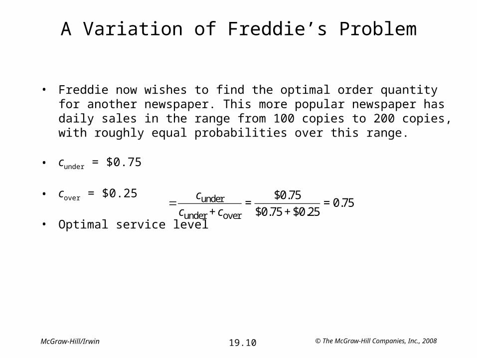
A Variation of Freddie’s Problem
• Freddie now wishes to find the optimal order quantity for another newspaper. This more popular newspaper has daily sales in the range from 100 copies to 200 copies, with roughly equal probabilities over this range.
• cunder = $0.75
• cover = $0.25
• Optimal service level=
cunder
cunder + cover=
$0.75
$0.75 + $0.25= 0.75.
© The McGraw-Hill Companies, Inc., 200819.11McGraw-Hill/Irwin
Graphical Application of the Ordering Rule
© The McGraw-Hill Companies, Inc., 200819.12McGraw-Hill/Irwin
Some Types of Perishable Products
• Periodicals, such as newspapers and magazines.
• Flowers being sold by a florist.
• The makings of fresh food to be prepared in a restaurant.
• Produce, including fresh fruits and vegetables, to be sold in a grocery store.
• Christmas trees.
• Seasonal clothing, such as winter coats, where any goods remaining at the end of the season must be sold at highly discounted prices to clear space for next season.
• Seasonal greeting cards.
• Fashion goods that will be out of style soon.
• New cars at the end of a model year.
• Any product that will be obsolete soon.
• Vital spare parts that must be produced during the last production run of a certain model of a product for use as needed throughout the lengthy field life of that model.
• Reservations provided by an airline for a particular flight. Reservations provided in excess of the number of seats available (overbooking) can be viewed as the inventory of a perishable product.
© The McGraw-Hill Companies, Inc., 200819.13McGraw-Hill/Irwin
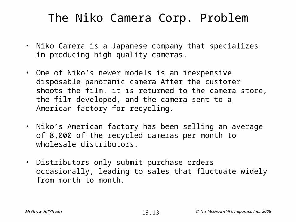
The Niko Camera Corp. Problem
• Niko Camera is a Japanese company that specializes in producing high quality cameras.
• One of Niko’s newer models is an inexpensive disposable panoramic camera After the customer shoots the film, it is returned to the camera store, the film developed, and the camera sent to a American factory for recycling.
• Niko’s American factory has been selling an average of 8,000 of the recycled cameras per month to wholesale distributors.
• Distributors only submit purchase orders occasionally, leading to sales that fluctuate widely from month to month.

© The McGraw-Hill Companies, Inc., 200819.14McGraw-Hill/Irwin
Monthly Sales for the Past Year
1
2
3
4
5
6
7
8
9
10
11
12
13
14
15
16
A B C D E
Monthly Sales of Niko's Disposable Cameras
Month Sales
January 7,000
February 1,500
March 15,800
April 8,600
May 9,900
June 4,200
July 13,600
August 700
September 14,100
October 6,200
November 5,000
December 9,400
© The McGraw-Hill Companies, Inc., 200819.15McGraw-Hill/Irwin
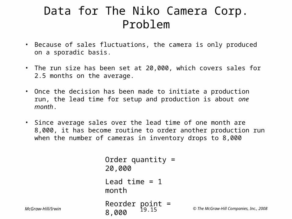
Data for The Niko Camera Corp. Problem
• Because of sales fluctuations, the camera is only produced on a sporadic basis.
• The run size has been set at 20,000, which covers sales for 2.5 months on the average.
• Once the decision has been made to initiate a production run, the lead time for setup and production is about one month.
• Since average sales over the lead time of one month are 8,000, it has become routine to order another production run when the number of cameras in inventory drops to 8,000
Order quantity = 20,000
Lead time = 1 month
Reorder point = 8,000

© The McGraw-Hill Companies, Inc., 200819.16McGraw-Hill/Irwin
Last Year’s Experience
1
2
3
4
5
6
7
8
9
10
11
12
13
14
15
16
17
18
19
20
21
22
23
24
25
26
27
28
29
30
31
32
33
A B C D E F G
Monthly Record of Niko's Inventory of Disposable Cameras
Beginning Ending
Month Sales Inventory Inventory Action
January 7,000 16,500 9,500 None
February 1,500 9,500 8,000 Ordered 20,000 at end of month
March 15,800 8,000 12,200 Order received at end of month
April 8,600 12,200 3,600 Ordered 20,000 during month
May 9,900 3,600 13,700 Order received during month
June 4,200 13,700 9,500 None
July 13,600 9,500 -4,100 Ordered 20,000 during month
August 700 -4,100 15,200 Order received during month
September 14,100 15,200 1,100 Ordered 20,000 during month
October 6,200 1,100 14,900 Order received during month
November 5,000 14,900 9,900 None
December 9,400 9,900 500 Ordered 20,000 during month
-15,000
-10,000
-5,000
0
5,000
10,000
15,000
20,000
January
February
March
April
MayJune July
August
September
October
November December
Time
Inventory Level

© The McGraw-Hill Companies, Inc., 200819.17McGraw-Hill/Irwin
Inventory Level

© The McGraw-Hill Companies, Inc., 200819.18McGraw-Hill/Irwin
Management Concerns
• Several distributors have complained about delays in shipping.
• Complaints have been received from the production floor about frequent interruptions in the production of other models caused by setting up for a production run for the disposable panoramic camera every two or three months.
• Proposal: have much longer production runs much less frequently.– This would provide larger inventories to reduce delayed shipments.
– This would substantially reduce setups and the associated disruptions.
– However, the larger inventories come at a cost.
• What should be done?
© The McGraw-Hill Companies, Inc., 200819.19McGraw-Hill/Irwin
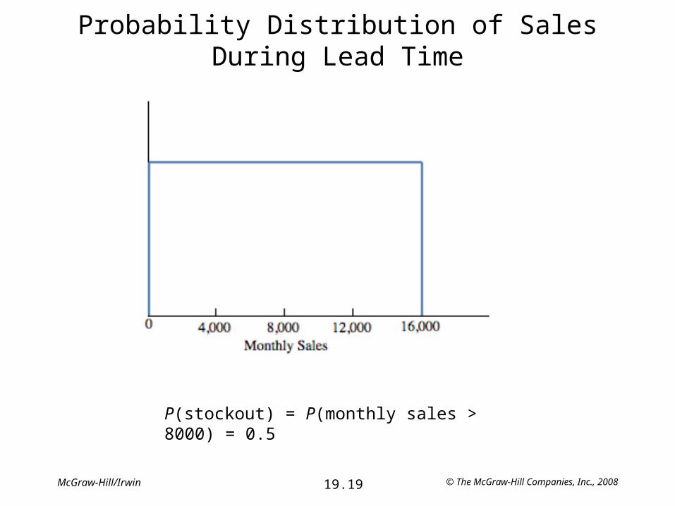
Probability Distribution of Sales During Lead Time
P(stockout) = P(monthly sales > 8000) = 0.5
© The McGraw-Hill Companies, Inc., 200819.20McGraw-Hill/Irwin
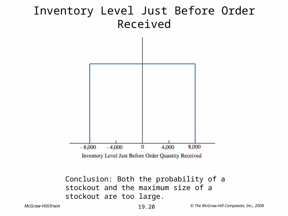
Inventory Level Just Before Order Received
Conclusion: Both the probability of a stockout and the maximum size of a stockout are too large.
© The McGraw-Hill Companies, Inc., 200819.21McGraw-Hill/Irwin
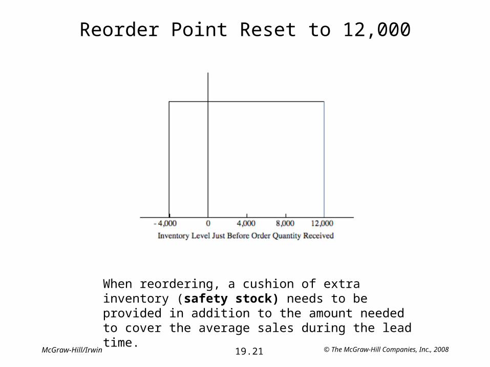
Reorder Point Reset to 12,000
When reordering, a cushion of extra inventory (safety stock) needs to be provided in addition to the amount needed to cover the average sales during the lead time.
© The McGraw-Hill Companies, Inc., 200819.22McGraw-Hill/Irwin
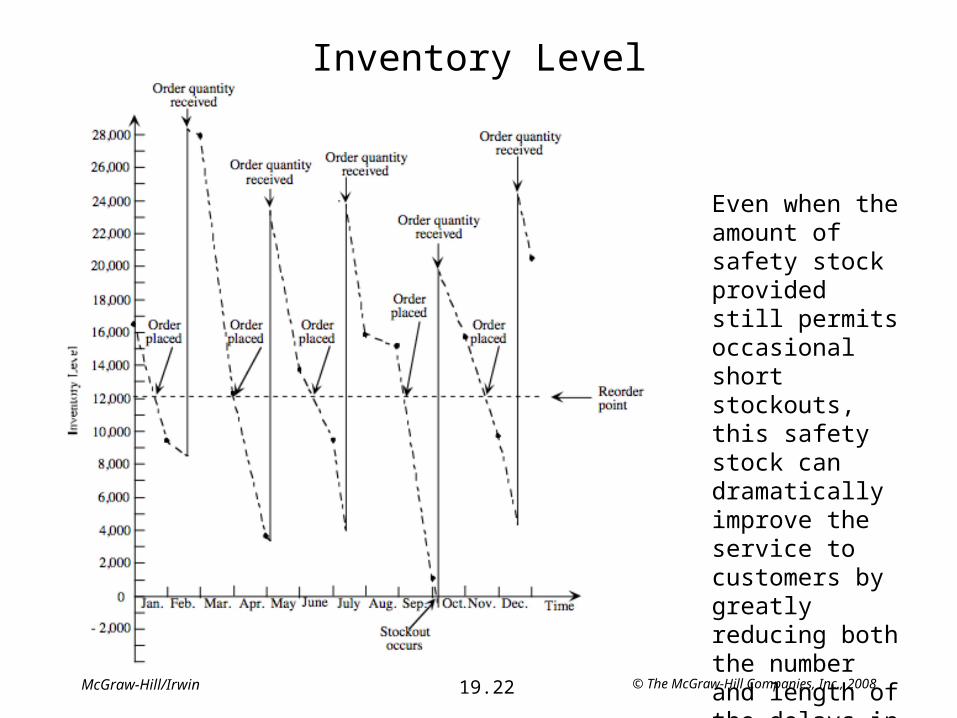
Inventory Level
Even when the amount of safety stock provided still permits occasional short stockouts, this safety stock can dramatically improve the service to customers by greatly reducing both the number and length of the delays in filling customer orders.
© The McGraw-Hill Companies, Inc., 200819.23McGraw-Hill/Irwin
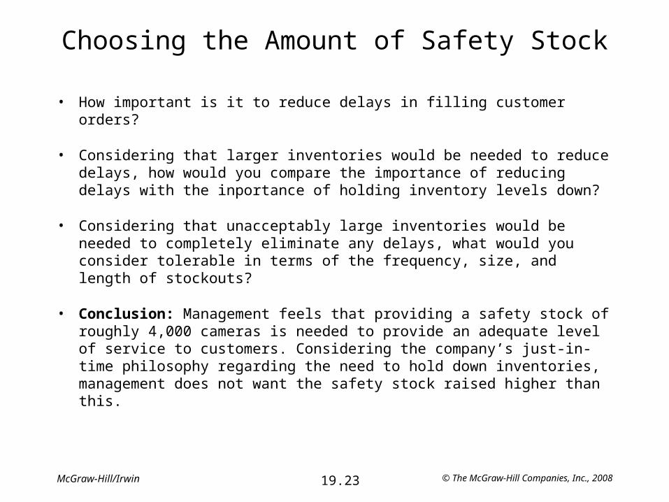
Choosing the Amount of Safety Stock
• How important is it to reduce delays in filling customer orders?
• Considering that larger inventories would be needed to reduce delays, how would you compare the importance of reducing delays with the inportance of holding inventory levels down?
• Considering that unacceptably large inventories would be needed to completely eliminate any delays, what would you consider tolerable in terms of the frequency, size, and length of stockouts?
• Conclusion: Management feels that providing a safety stock of roughly 4,000 cameras is needed to provide an adequate level of service to customers. Considering the company’s just-in-time philosophy regarding the need to hold down inventories, management does not want the safety stock raised higher than this.

© The McGraw-Hill Companies, Inc., 200819.24McGraw-Hill/Irwin
The Cost Factors
• Acquisition Cost – This cost ($7 per camera) is irrelevant when choosing the order quantity.
– The order quantity only affects the timing of production/acquisition cost.
• Setup Cost– The cost of setting up a production run is $12,000.
– The order quantity determines how frequently the setup cost will be incurred.
• Holding Cost– The cost of space, record keeping, protection, insurance, and taxes is estimated 10¢
per camera per month.
– The cost of capital tied up is estimated at 20¢ per camera per month.
– Hence, it is assumed the total holding cost per month is 30¢ times the inventory level.
• Shortage Cost– Estimated to be about $10 per camera per month of delay.
© The McGraw-Hill Companies, Inc., 200819.25McGraw-Hill/Irwin
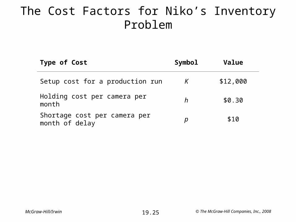
The Cost Factors for Niko’s Inventory Problem
Type of Cost Symbol Value
Setup cost for a production run K $12,000
Holding cost per camera per month h $0.30
Shortage cost per camera per month of delay p $10
© The McGraw-Hill Companies, Inc., 200819.26McGraw-Hill/Irwin
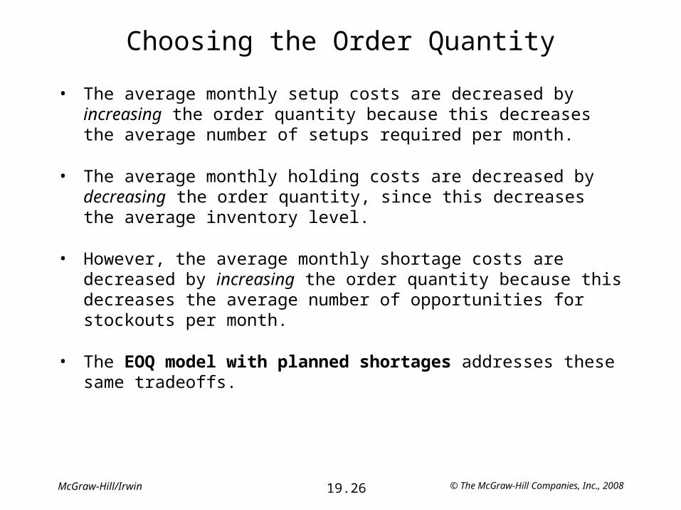
Choosing the Order Quantity
• The average monthly setup costs are decreased by increasing the order quantity because this decreases the average number of setups required per month.
• The average monthly holding costs are decreased by decreasing the order quantity, since this decreases the average inventory level.
• However, the average monthly shortage costs are decreased by increasing the order quantity because this decreases the average number of opportunities for stockouts per month.
• The EOQ model with planned shortages addresses these same tradeoffs.
© The McGraw-Hill Companies, Inc., 200819.27McGraw-Hill/Irwin
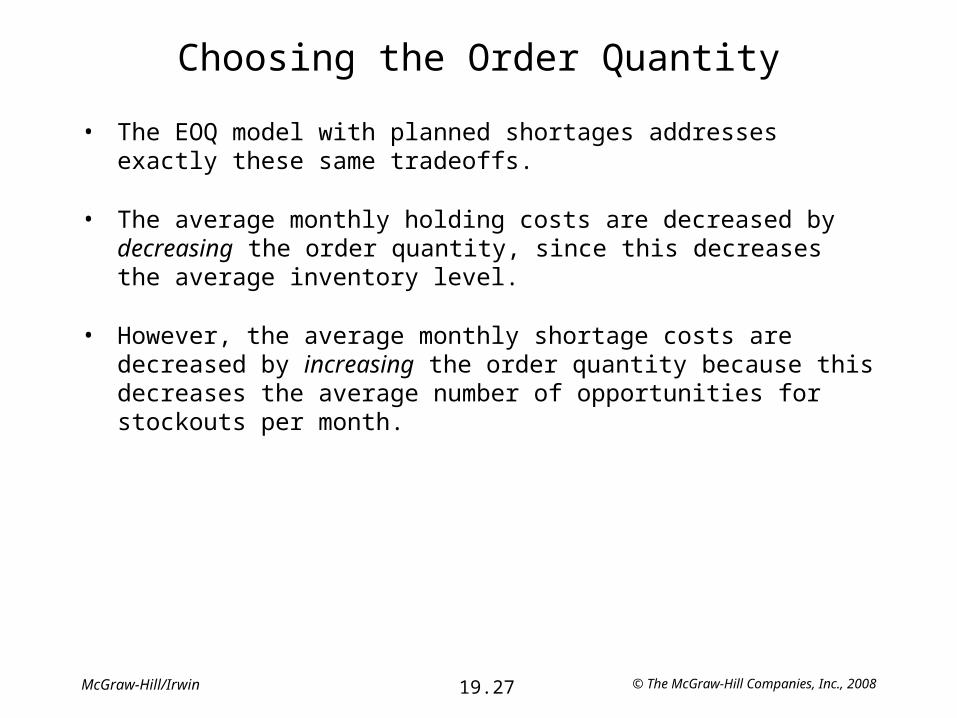
Choosing the Order Quantity
• The EOQ model with planned shortages addresses exactly these same tradeoffs.
• The average monthly holding costs are decreased by decreasing the order quantity, since this decreases the average inventory level.
• However, the average monthly shortage costs are decreased by increasing the order quantity because this decreases the average number of opportunities for stockouts per month.
© The McGraw-Hill Companies, Inc., 200819.28McGraw-Hill/Irwin
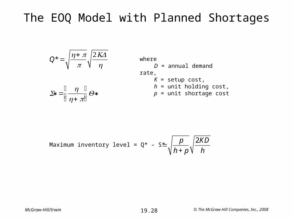
The EOQ Model with Planned Shortages
Q* =h+ p
p2KD
h
S* =h
h+ p⎛⎝⎜
⎞⎠⎟Q*
whereD = annual demand rate,K = setup cost,h = unit holding cost,p = unit shortage cost
Maximum inventory level = Q* – S* =p
h + p
2KD
h

© The McGraw-Hill Companies, Inc., 200819.29McGraw-Hill/Irwin
The EOQ Model with Planned Shortages
Range Name Cell
AnnualHoldingCost G7
AnnualSetupCost G6
AnnualShortageCost G8
D C4
h C6
K C5
MaxInventoryLevel G4
p C7
Q C10
S C11
TotalVariableCost G9
4
5
6
7
8
9
F G
Max Inventory Level =Q-S
Annual Setup Cost =K*D/Q
Annual Holding Cost =h*(MaxInventoryLevel^2)/(2*Q)
Annual Shortage Cost =p*((Q-MaxInventoryLevel)^2)/(2*Q)
Total Variable Cost =AnnualSetupCost+AnnualHoldingCost+AnnualShortageCost
10
11
B C
Q = =SQRT(2*D*K/h)*SQRT((p+h)/p)
S = =(h/(h+p))*Q
123456789
1011
A B C D E F G
EOQ Model with Planned Shortages (Niko Case Study)
Data ResultsD = 8000 (demand/year) Max Inventory Level 24927.08K = $12,000 (setup cost)h = $0.30 (unit holding cost) Annual Setup Cost $3,739.06p = $10 (unit shortage cost) Annual Holding Cost $3,630.16
Annual Shortage Cost $108.90Decision Total Variable Cost $7,478.12
Q = 25675 (order quantity)S = 748 (maximum shortage)
© The McGraw-Hill Companies, Inc., 200819.30McGraw-Hill/Irwin
Niko’s Inventory Level
© The McGraw-Hill Companies, Inc., 200819.31McGraw-Hill/Irwin
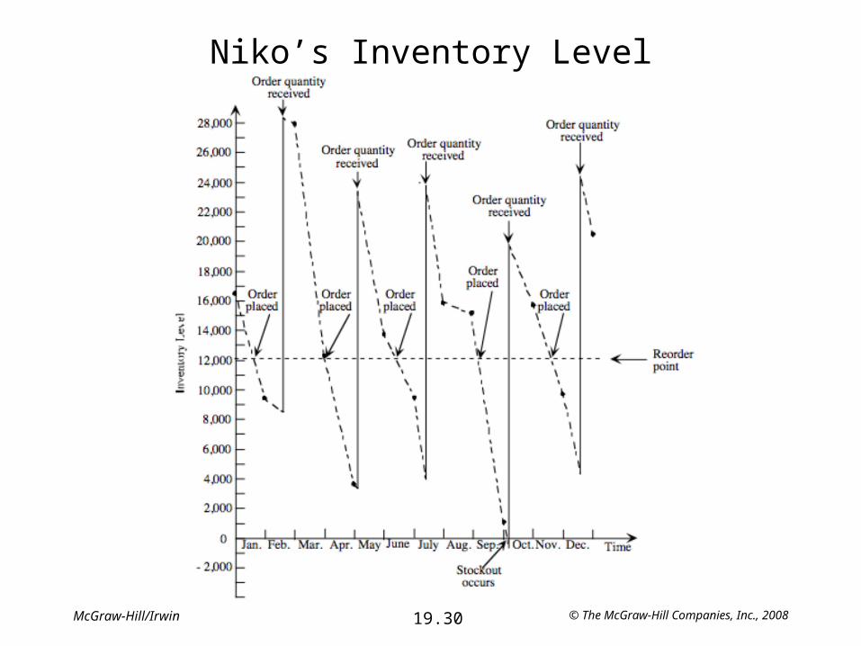
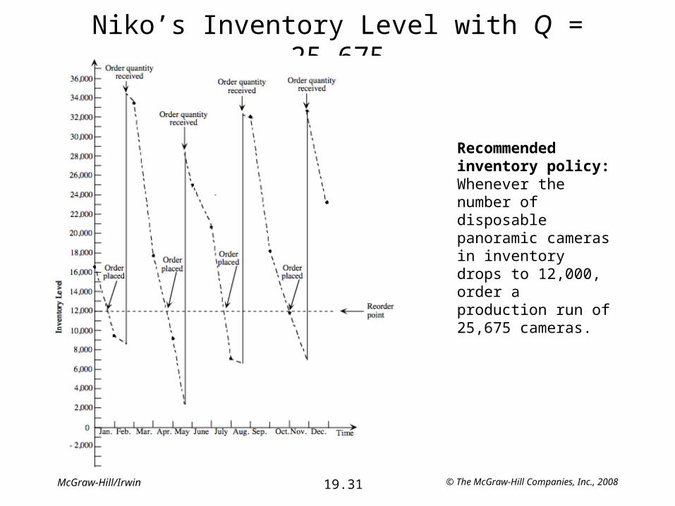
Niko’s Inventory Level with Q = 25,675
Recommended inventory policy: Whenever the number of disposable panoramic cameras in inventory drops to 12,000, order a production run of 25,675 cameras.
© The McGraw-Hill Companies, Inc., 200819.32McGraw-Hill/Irwin
Additional Recommendations from the Team
• Acquire some additional production facilities that would be used solely for the production runs of the disposable panoramic camera as needed
• Provide a small price incentive to the company’s customers to place a standing order for regular monthly purchases.
• Develop a system of coordinating sales of the disposable panoramic camera as needed with the company’s divisions in other parts of the world.
• A study also should be conducted of the raw material inventories, including especially the returned reusable components.
© The McGraw-Hill Companies, Inc., 200819.33McGraw-Hill/Irwin
A Continuous-Review Inventory Model
• The model is for stable products (products that will remain sellable indefinitely) as opposed to perishable products (sellable for only a limited time).
• The model is a continuous-review model because it assumes inventory level is monitored on a continuous basis so that a new order can be placed as soon as the inventory level drops to the reorder point. This is as opposed to a periodic-review inventory system where the inventory level is only monitored periodically such as at the end of each week.
• The traditional method of implementing a continuous-review inventory system was to use a two-bin system. All the units would be held in two bins. The capacity of one bin would equal the reorder point. The units would be withdrawn from the other bin until empty, triggering a reorder.
• In more recent years, two-bin systems have been largely replaced by computerized inventory systems where each sale is recorded electronicaly, so that the current inventory level is always in the computer.
© The McGraw-Hill Companies, Inc., 200819.34McGraw-Hill/Irwin
A Continuous-Review Inventory System
• A continuous-review inventory system will be based on two critical numbers:– R = reorder point– Q = order quantity
• Inventory policy: Whenever the inventory level of the product drops to R units, place an order for Q more units to replenish the inventory.

© The McGraw-Hill Companies, Inc., 200819.35McGraw-Hill/Irwin
Assumptions of the Model
• Each application involves a single stable product
• The inventory level is under continuous review, so its current value is always known.
• An (R, Q) policy is to be used, so the only decisions are to choose R and Q.
• There is a lead time (either fixed or variable) between when the order is placed and received.
• The demand for withdrawing units from inventory is uncertain. However, the probability distribution of demand is known (or estimated).
• If a stockout occurs before the order is received, excess demand is backlogged.
• A fixed setup cost (denoted by K) is incurred each time an order is placed.
• Except for this setup cost, the cost of the order is proportional to the order quantity Q.
• A certain holding cost (denoted by h) is incurred for each unit in inventory per unit time.
• When a stockout occurs, a certain shortage cost (denoted by p) is incurred for each unit backordered per unit time until the backorder is filled.

© The McGraw-Hill Companies, Inc., 200819.36McGraw-Hill/Irwin
Choosing the Order Quantity
The most straightforward approach to choosing Q is to simply use the formula for the EOQ model with planned shortages:
Q* =h+ p
p2KD
h
© The McGraw-Hill Companies, Inc., 200819.37McGraw-Hill/Irwin
Choosing the Reorder Point
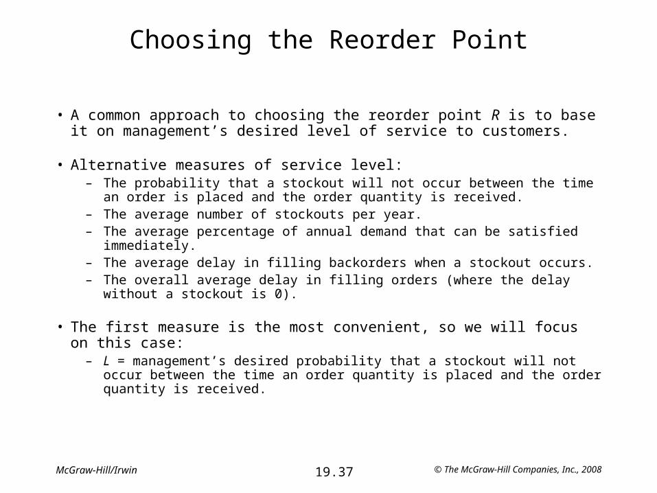
• A common approach to choosing the reorder point R is to base it on management’s desired level of service to customers.
• Alternative measures of service level:– The probability that a stockout will not occur between the time an order is placed
and the order quantity is received.– The average number of stockouts per year.– The average percentage of annual demand that can be satisfied immediately.– The average delay in filling backorders when a stockout occurs.– The overall average delay in filling orders (where the delay without a stockout is 0).
• The first measure is the most convenient, so we will focus on this case:– L = management’s desired probability that a stockout will not occur between the
time an order quantity is placed and the order quantity is received.
© The McGraw-Hill Companies, Inc., 200819.38McGraw-Hill/Irwin
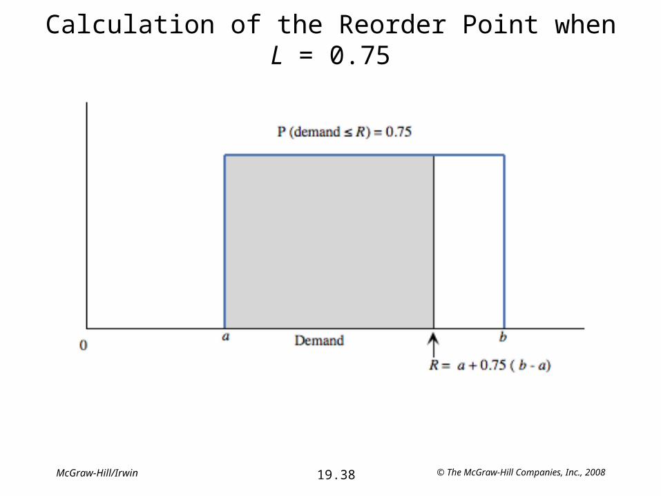
Calculation of the Reorder Point when L = 0.75

© The McGraw-Hill Companies, Inc., 200819.39McGraw-Hill/Irwin
Calculating R for a Normal Demand Distribution
L KL
0.5 0
0.6 0.253
0.7 0.524
0.75 0.675
0.8 0.842
0.85 1.037
0.9 1.282
0.95 1.645
0.975 1.960
0.99 2.327
0.995 2.576
0.999 3.098
© The McGraw-Hill Companies, Inc., 200819.40McGraw-Hill/Irwin
General Procedure for Choosing R
• Choose L = probability that a stockout will not occur between the time an order quantity is placed and the order quantity is received.
• Solve for R such thatP (demand ≤ R) = L.

© The McGraw-Hill Companies, Inc., 200819.41McGraw-Hill/Irwin
Optimal Ordering Policy
Range Name Cell
a C13
b C14
D C4
Distribution C12
h C6
K C5
L C8
Mean C13
OrderQuantity G4
p C7
ReorderPoint G5
StandardDeviation C14
4
5
F G
Q = =SQRT(2*D*K/h)*SQRT((p+h)/p)
R = =IF(Distribution="Uniform",a+L*(b-a),NORMINV(L,Mean,StandardDeviation))
1
2
3
4
5
6
7
8
9
10
11
12
13
14
A B C D E F G
Optimal Ordering Policy for Stable Products (Uniform Distribution)
Data Results
D = 8000 (average demand/unit time) Q = 25,675
K = $12,000 (setup cost) R = 12,000
h = $0.30 (unit holding cost)
p = $10 (unit shortage cost)
L = 0.75 (service level)
Demand During Lead Time
Distribution Uniform
a = 0 (lower endpoint)
b = 16,000 (upper endpoint)
© The McGraw-Hill Companies, Inc., 200819.42McGraw-Hill/Irwin
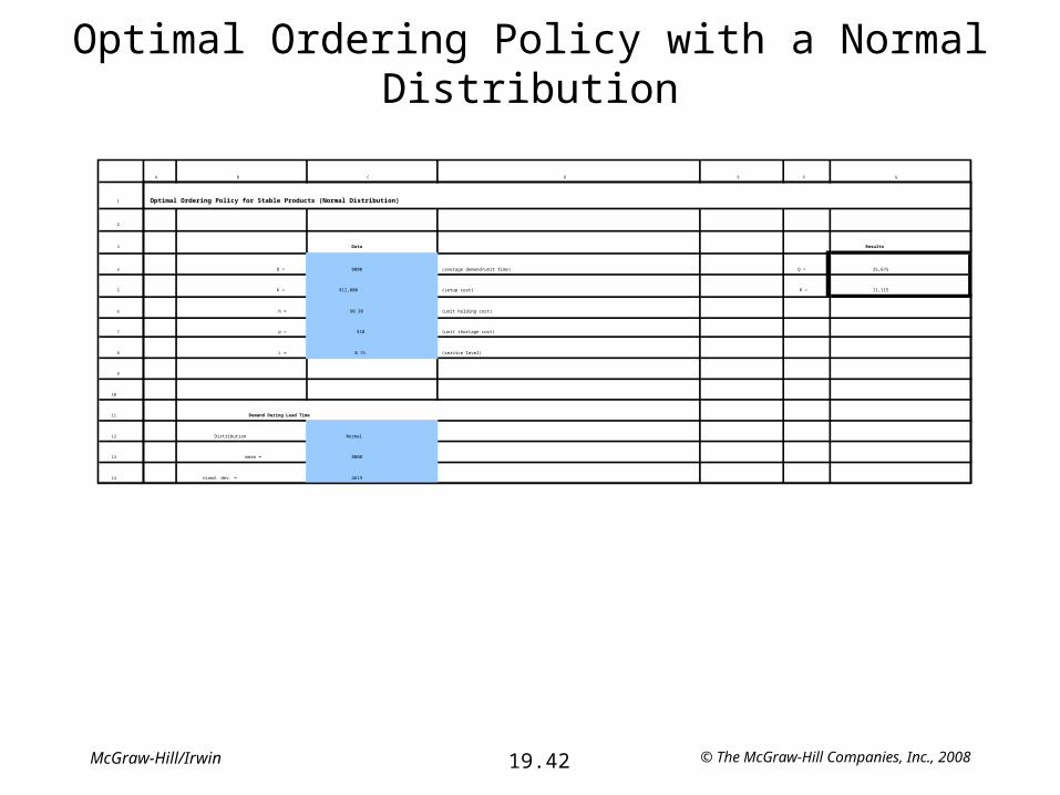
Optimal Ordering Policy with a Normal Distribution
1
2
3
4
5
6
7
8
9
10
11
12
13
14
A B C D E F G
Optimal Ordering Policy for Stable Products (Normal Distribution)
Data Results
D = 8000 (average demand/unit time) Q = 25,675
K = $12,000 (setup cost) R = 11,115
h = $0.30 (unit holding cost)
p = $10 (unit shortage cost)
L = 0.75 (service level)
Demand During Lead Time
Distribution Normal
mean = 8000
stand. dev. = 4619
© The McGraw-Hill Companies, Inc., 200819.43McGraw-Hill/Irwin
Larger Inventory Systems in Practice• Multiproduct Inventory Systems
– It is common to apply the appropriate single-product model to each product individually.
– The ABC Control Method is commonly applied to divide the products into categories, where the A group must be monitored carefully while the C group need only be informally monitored.
– It may not be appropriate to apply the single-product model if there are interactions between products.
• Multi-Echelon Inventory Systems– Inventory may be stored initially at the points of manufacture (one echelon), then at
regional warehouses (a second echelon), then at field distribution centers (a third echelon), etc.
– Some coordination is needed between the inventories at the different echelon.
• Supply Chain Management– A supply chain is a network of facilities that procure raw materials, transform them
into intermediate goods and then final products, and finally deliver the products to customers through a distribution system that includes a (probably multiechelon) inventory system.
– To fill orders efficiently, it is necessary to understand the linkages and interrelationships of all the key elements of the supply chain.