McDonald 2ePPT CH20

Chapter 20

Brownian Motion and Itô’s Lemma

Copyright © 2006 Pearson Addison-Wesley. All rights reserved. 20-2

Introduction

• Stock and other asset prices are commonly assumed to follow a stochastic process called geometric Brownian motion

• Given that a stock price follows geometric Brownian motion, we want to characterize the behavior of a claim that has a payoff dependent upon the stock price We will discuss Itô’s Lemma, which permits us to

study the process followed by a claim that is a function of the stock price


)( )()( tdZdttStdS

The Black-Scholes Assumption About Stock Prices

• The original paper by Black and Scholes begins by assuming that the price of the underlying asset follows a process like the following

(20.1)where

S(t) is the stock price dS(t) is the instantaneous change in the stock price is the continuously compounded expected return on the stock is the continuously compounded standard deviation (volatility) Z(t) is a normally distributed random variable that follows a process

called Brownian motion dZ(t) is the change in Z(t) over a short period of time


The Black-Scholes Assumption About Stock Prices (cont’d)

• A stock obeying equation (20.1) is said to follow a process called geometric Brownian motion

• Expressions like equation (20.1) are called stochastic differential equations

• There are 2 important implications of equation (20.1) Suppose the stock price now is S(0). If the stock price follows

equation (20.1), the distribution of S(T) is lognormal, i.e.

Geometric Brownian motion allows us to describe the path the stock price takes in getting to a terminal point

In[S(T )] ~ N(In[S(O)] [ 0.5 2 ]T , 2T )


A Description of Stock Price Behavior

• The normal distribution provides an unrealistic description of the stock price. However, normality can be a plausible description of continuously compounded returns If the continuously compounded return is R(0,T),

the price is S(0) eR(0,T), which is always positive

• It can be reasonable to assume that over very short periods of time effective stock returns, S(t + h)/S(t), are normally distributed


A Description of Stock Price Behavior (cont’d)

• Suppose that h, the length of each time period, is small, the return on the stock, rh, is normally

distributed with mean and variance h and 2h

• Thus,

with

S(t h) S(t)(1 rh )

rh ~ N(h, 2h)


n

i ihrlnSTSln

1 )1()]0(/)([

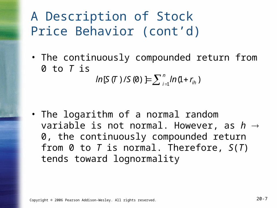
A Description of Stock Price Behavior (cont’d)

• The continuously compounded return from 0 to T is

• The logarithm of a normal random variable is not normal. However, as h 0, the continuously compounded return from 0 to T is normal. Therefore, S(T) tends toward lognormality


Brownian Motion

• Brownian motion is a random walk occurring in continuous time, with movements that are continuous rather than discrete A random walk can be generated by flipping a coin

each period and moving one step, with the direction determined by whether the coin is heads or tails

To generate Brownian motion, we would flip the coins infinitely fast and take infinitesimally small steps at each point


Brownian Motion (cont’d)

• Let Z(t) represent the value of the random walk—the cumulative sum of all the moves—after t periods

• Technically, Brownian motion is a random walk with the following characteristics

Z(0) = 0 Z(t + s) – Z (t) is normally distributed with mean 0

and variance s Z(t + s1) – Z(t) is independent of Z(t) – Z(t – s2), where

s1, s2 >0. That is, nonoverlapping increments are independently distributed

Z(t) is continuous



• We can think of Brownian motion being approximately generated from the sum of independent binomial draws with mean 0 and variance h

• Let h get arbitrarily small, and rename h as dt. Denote the change in Z as dZ(t)


dttYtdZ )()(


• Then

(20.4) where Y(t) is a random draw from a binomial

distribution, such that Y(t) is 1 with probability 50%

• Equation (20.4) says “Over small periods of time, changes in the value of the process are normally distributed with a variance that is proportional to the length of the time period.”


T

tdZZTZ0

)()0()(


• Since Z(T) is the sum of individual dZ(t)’s, we can write

The integral here is called a stochastic integral The process Z(t) is also called a diffusion process

• Among properties of Brownian motion are “infinite-crossing property” and “infinite variation”


)( )( tdZdttdX

Arithmetic Brownian Motion

• With pure Brownian motion, the expected change in Z is 0, and the variance per unit time is 1. We can generalize this to allow an arbitrary variance and a nonzero mean

(20.8)

• This process is called arithmetic Brownian motion is the instantaneous mean per unit time

2 is the instantaneous variance per unit time

The variable X(t) is the sum of the individual changes dX. X(t) is normally distributed, i.e., X(T) – X(0) ~ N (T, 2T)


TT

tdZdtXTX00

)( )0()(

Arithmetic Brownian Motion (cont’d)

• An integral representation of equation (20.8) is

• Here are some properties of the process in equation (20.8) X(t) is normally distributed because it is created by

adding together many normally distributed dX’s The random term is multiplied by a scale factor that

enables us to change variance The dt term introduces a nonrandom drift into

the process


Arithmetic Brownian Motion (cont’d)

• Arithmetic Brownian motion has several drawbacks There is nothing to prevent X from becoming

negative, so it is a poor model for stock prices The mean and variance of changes in dollar terms

are independent of the level of the stock price

• Both of these criticisms will be eliminated with geometric Brownian motion


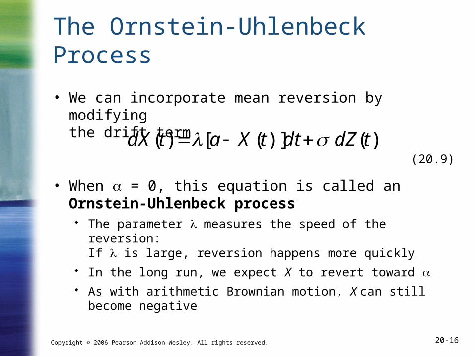
)( )]([)( tdZdttXatdX

The Ornstein-Uhlenbeck Process

• We can incorporate mean reversion by modifying the drift term

(20.9)

• When = 0, this equation is called an Ornstein-Uhlenbeck process

The parameter measures the speed of the reversion: If is large, reversion happens more quickly

In the long run, we expect X to revert toward As with arithmetic Brownian motion, X can still

become negative


)( )()( tdZdtatXtdX

)()( )( )( tdZtXdttXatdX

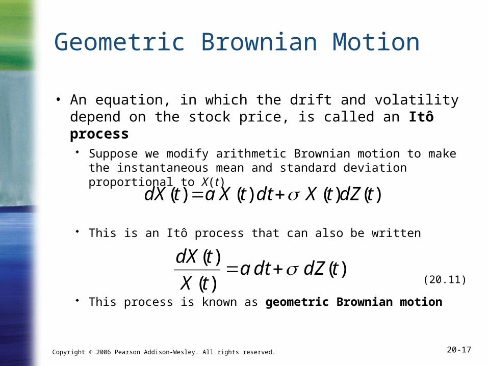
Geometric Brownian Motion

• An equation, in which the drift and volatility depend on the stock price, is called an Itô process

Suppose we modify arithmetic Brownian motion to make the instantaneous mean and standard deviation proportional to X(t)

This is an Itô process that can also be written

(20.11)

This process is known as geometric Brownian motion


TT

tdZtXdttXXTX00

)()( )( )0()(

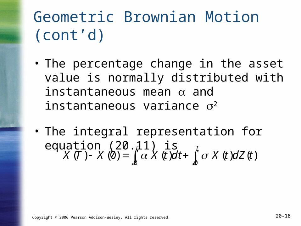
Geometric Brownian Motion (cont’d)

• The percentage change in the asset value is normally distributed with instantaneous mean and instantaneous variance 2

• The integral representation for equation (20.11) is


Lognormality

• If a variable is distributed in such a way that instantaneous percentage changes follow geometric Brownian motion, then over discrete periods of time, the variable is lognormally distributed


hhtXhtX

)(

)(

Relative Importance of the Drift and Noise Terms

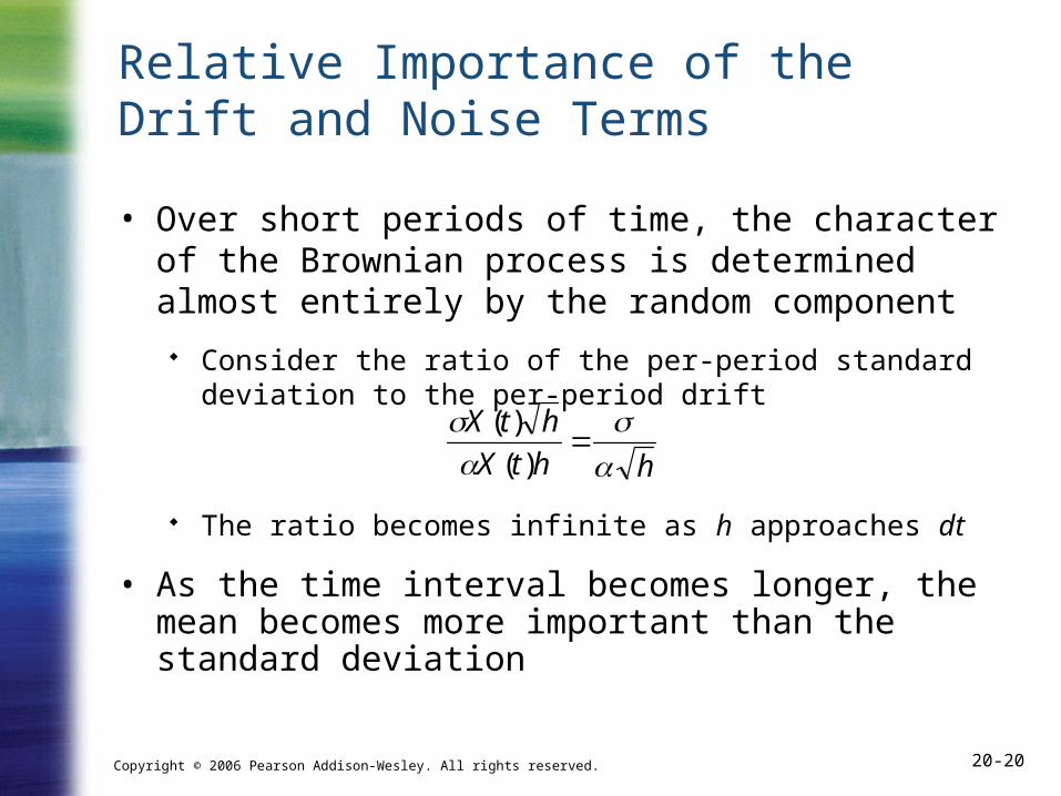
• Over short periods of time, the character of the Brownian process is determined almost entirely by the random component

Consider the ratio of the per-period standard deviation to the per-period drift

The ratio becomes infinite as h approaches dt

• As the time interval becomes longer, the mean becomes more important than the standard deviation


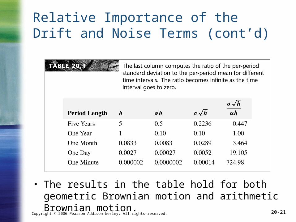
Relative Importance of the Drift and Noise Terms (cont’d)

• The results in the table hold for both geometric Brownian motion and arithmetic Brownian motion.


)(1)()(

)()(

22

1

1

tWtWtZ

tWtZ'

0 )]()([1])([)]()([ 2122

1 ttWtWEtWEtZtZE '

Correlated Itô Processes

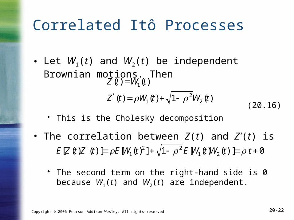
• Let W1(t) and W2(t) be independent Brownian motions. Then

(20.16) This is the Cholesky decomposition

• The correlation between Z(t) and Z'(t) is

The second term on the right-hand side is 0 because W1(t) and W2(t) are independent.


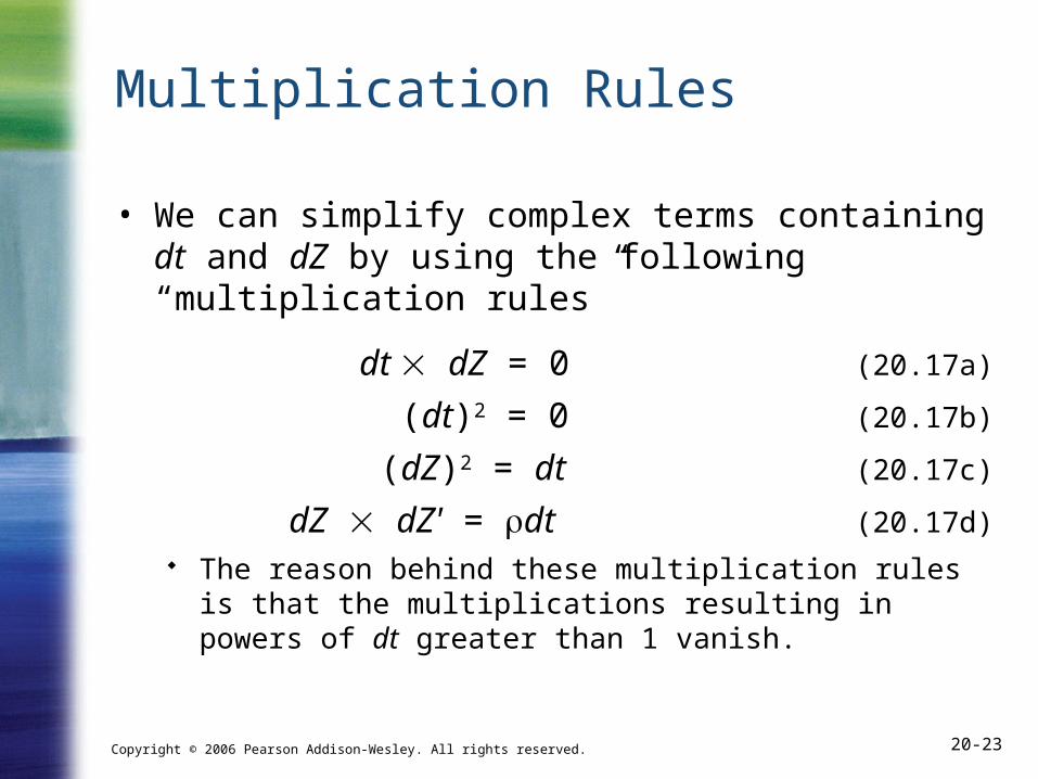
Multiplication Rules

• We can simplify complex terms containing dt and dZ by using the following “multiplication rules”

dt dZ = 0 (20.17a)

(dt)2 = 0 (20.17b)

(dZ)2 = dt (20.17c)

dZ dZ' = dt (20.17d) The reason behind these multiplication rules is that the

multiplications resulting in powers of dt greater than 1 vanish.


i

ii

rα

ratio Sharpe

The Sharpe Ratio

• If asset i has expected return i, the risk premium is defined as

Risk premiumi = i – r where r is the risk-free rate

• The Sharpe ratio for asset i is the risk premium, i – r, per unit of volatility, I

(20.18)


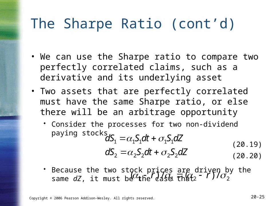
The Sharpe Ratio (cont’d)

• We can use the Sharpe ratio to compare two perfectly correlated claims, such as a derivative and its underlying asset

• Two assets that are perfectly correlated must have the same Sharpe ratio, or else there will be an arbitrage opportunity

Consider the processes for two non-dividend paying stocks(20.19)(20.20)

Because the two stock prices are driven by the same dZ, it must be the case that

dS1 1S1dt 1S1dZdS2 2S2dt 2S2dZ

(1 r) / 1 (2 r) / 2


)()()()( tdZdttStdS

)( )()()( * tdZdtrtStdS

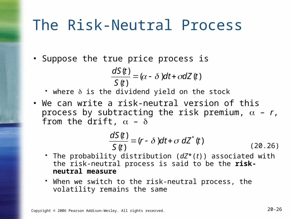
The Risk-Neutral Process

• Suppose the true price process is

where is the dividend yield on the stock

• We can write a risk-neutral version of this process by subtracting the risk premium, – r, from the drift, –

(20.26) The probability distribution (dZ*(t)) associated with the risk-

neutral process is said to be the risk-neutral measure When we switch to the risk-neutral process, the volatility

remains the same


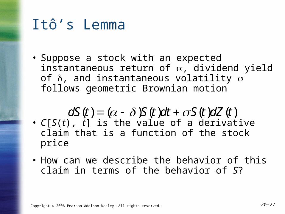
Itô’s Lemma

• Suppose a stock with an expected instantaneous return of , dividend yield of , and instantaneous volatility follows geometric Brownian motion

• C[S(t), t] is the value of a derivative claim that is a function of the stock price

• How can we describe the behavior of this claim in terms of the behavior of S?

dS(t) ( )S(t)dt S(t)dZ(t)


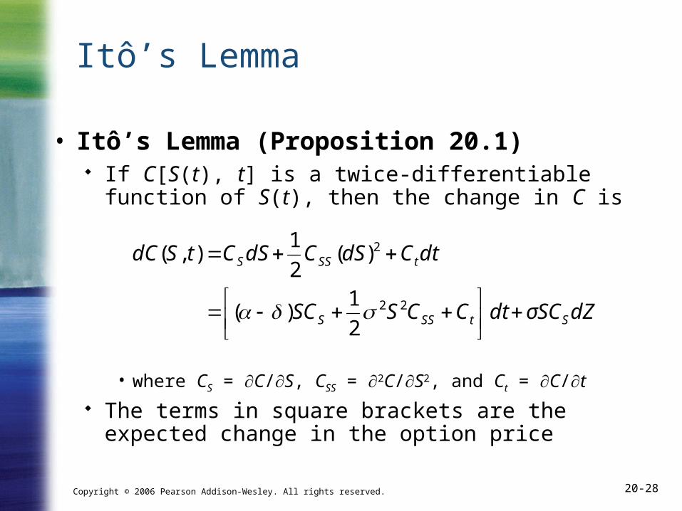
Itô’s Lemma

• Itô’s Lemma (Proposition 20.1) If C[S(t), t] is a twice-differentiable function of S(t), then

the change in C is

• where CS = C/S, CSS = 2C/S2, and Ct = C/t The terms in square brackets are the expected change

in the option price

dZσSCdtCCSSC

dtCdSCdSCtSdC

StSSS

tSSS

21)(

)(21) ,(

22

2


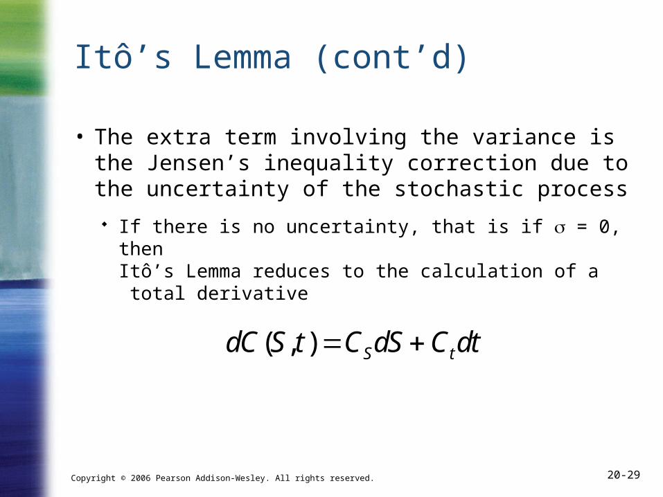
Itô’s Lemma (cont’d)

• The extra term involving the variance is the Jensen’s inequality correction due to the uncertainty of the stochastic process If there is no uncertainty, that is if = 0, then

Itô’s Lemma reduces to the calculation of a total derivative

dC(S, t) CSdS Ctdt


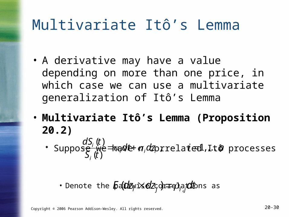
Multivariate Itô’s Lemma

• A derivative may have a value depending on more than one price, in which case we can use a multivariate generalization of Itô’s Lemma

• Multivariate Itô’s Lemma (Proposition 20.2) Suppose we have n correlated Itô processes

• Denote the pairwise correlations as

nidzdttStdS

iiii

i ., . . ,1 , )()(

E(dzi dz j ) i, jdt


n

i

n

i tn

j SSjiiSn dtCCdSdSdSCtSSdCjii1 1 11 2

1), ., . . ,(

n

i tn

j SSjiijjin

i Siin CCSSCStSSdCEdt jii 1 111 2

1)] , ., . . ,([1

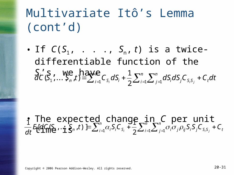
Multivariate Itô’s Lemma (cont’d)

• If C(S1, . . ., Sn, t) is a twice-differentiable function of the Si’s, we have

• The expected change in C per unit time is

McDonald 2ePPT CH20

Documents

Transcript of McDonald 2ePPT CH20