May 22, 2013 Ronald Reagan Building and International ... · Ronald Reagan Building and...
53
Copyright © 2013, Oracle and/or its affiliates. All rights reserved. 1 May 22, 2013 Ronald Reagan Building and International Trade Center Washington, DC USA
Transcript of May 22, 2013 Ronald Reagan Building and International ... · Ronald Reagan Building and...

Copyright © 2013, Oracle and/or its affiliates. All rights reserved. 1
May 22, 2013 Ronald Reagan Building and International Trade Center
Washington, DC USA

Performance, Performance, Performance What You Need To Know About Exadata Daniel Geringer Senior Software Development Manager
To fill a shape with an image.
1. Use existing picture box, DO NOT delete and create
2. Right click on the shape. 3. At the bottom of the submenu select
4. Select “Fill” at the top of the “Format Shape” dialog
5. Select “Picture or Texture fill” from the options. 6. And select “File” under the “Insert from” option. 7. Navigate to the file you want to use and
8. On the “Format” tab, in the Size group, click on
9. DELETE THIS INSTRUCTION NOTE WHEN NOT

Copyright © 2013, Oracle and/or its affiliates. All rights reserved. 3
The following is intended to outline our general product direction. It is intended for information purposes only, and may not be incorporated into any contract. It is not a commitment to deliver any material, code, or functionality, and should not be relied upon in making purchasing decisions. The development, release, and timing of any features or functionality described for Oracle’s products remains at the sole discretion of Oracle.

Copyright © 2013, Oracle and/or its affiliates. All rights reserved. 4
Program Agenda
Oracle Exadata Database Machine
Parallel Enabled Spatial Operators and Functions
Hybrid Columnar Compression (HCC) and Spatial
Massive Spatial Data Ingests with Spatial Index Enabled

Copyright © 2013, Oracle and/or its affiliates. All rights reserved. 5
Oracle Exadata Database Machine Engineered System

Copyright © 2013, Oracle and/or its affiliates. All rights reserved. 6
What Is the Oracle Exadata Database Machine? Oracle SUN hardware uniquely engineered to work together with
Oracle database software Key features:
– Database Grid – Up to 160 Intel cores connected by 40 Gb/second InfiniBand fabric, for massive parallel query processing.
– Raw Disk – Up to 504 TB of uncompressed storage (high performance or high capacity)
– Memory – Up to 2 TB – Hybrid Columnar Compression (HCC) – Query and archive modes
available. 3x to 30x compression. – Storage Servers – Up to 14 storage servers (168 Intel cores) that can
perform massive parallel smart scans. Smart scans offloads SQL predicate filtering to the raw data blocks. Results in much less data transferred, and dramatically improved performance.
– Flash memory – Up to 22.4 TB with I/O resource management

Copyright © 2013, Oracle and/or its affiliates. All rights reserved. 7
Exadata X3-2 Quarter Rack Diagram
3 TB storage 12 Xeon cores
RAC, OLAP Partitioning
Compression
Exadata DB Machine X3-2 Quarter Rack
16 Xeon cores 16 Xeon cores
3 TB storage 12 Xeon cores
3 TB storage 12 Xeon cores

Copyright © 2013, Oracle and/or its affiliates. All rights reserved. 8
Parallel Enabled Spatial Operators and Functions

Copyright © 2013, Oracle and/or its affiliates. All rights reserved. 9
Oracle Spatial and Graph Is Parallel Enabled
Parallel enabled Spatial Operators and Functions a major focus Designed for highly parallel architectures, like Exadata:
– Parallel spatial queries – Parallel spatial index creation – Parallel geometry validation – Parallel Geocoding – Parallel raster operations – Spatial batch spatial operations – And more…
Key Differentiator

Copyright © 2013, Oracle and/or its affiliates. All rights reserved. 10
Parallel Query and Spatial With Spatial Operators and Partitioned Tables

Copyright © 2013, Oracle and/or its affiliates. All rights reserved. 11
Parallel Query And Spatial Operators
If a spatial operator’s query window spans multiple partitions, partitions are spatially searched in parallel.
True for all spatial operators
Partitioned Tables
Copyright © 2013, Oracle and/or its affiliates. All rights reserved. 12
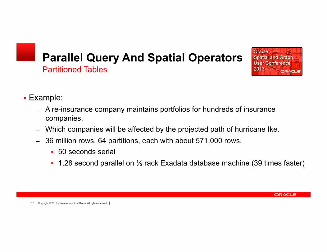
Parallel Query And Spatial Operators
Example: – A re-insurance company maintains portfolios for hundreds of insurance
companies. – Which companies will be affected by the projected path of hurricane Ike. – 36 million rows, 64 partitions, each with about 571,000 rows.
50 seconds serial 1.28 second parallel on ½ rack Exadata database machine (39 times faster)
Partitioned Tables

Copyright © 2013, Oracle and/or its affiliates. All rights reserved. 13
Parallel Query and Spatial With Spatial Operators

Copyright © 2013, Oracle and/or its affiliates. All rights reserved. 14
Parallel Query And Spatial Operators
Spatial operators can parallelize when multiple candidates feed the second argument

Copyright © 2013, Oracle and/or its affiliates. All rights reserved. 15
Parallel Query and Spatial US Rail Application

Copyright © 2013, Oracle and/or its affiliates. All rights reserved. 16
Parallel Query And Spatial Operators
Requirement – GPS locations for each train collected throughout the day – Each location has other attributes (time, speed, and more) – GPS locations have a degree of error, so they don’t always fall on a track. – Bulk nearest neighbor queries to find closest track, and project reported
train positions onto tracks
This information is used for: – Tracking trains – Analysis for maintenance, ensure engineers are within parameters,etc
US Rail Application

Copyright © 2013, Oracle and/or its affiliates. All rights reserved. 17
Parallel Query And Spatial Operators
• 45,158,800 GPS train positions. • For each train position:
• Find the closest track to the train (with SDO_NN) • Then calculate the position on the track closest to
the train
What we tested

Copyright © 2013, Oracle and/or its affiliates. All rights reserved. 18
Parallel Query and Spatial Operators US Rail Application ALTER SESSION FORCE PARALLEL ddl PARALLEL 72; ALTER SESSION FORCE PARALLEL query PARALLEL 72;
CREATE TABLE results NOLOGGING AS SELECT /*+ ordered index (b tracks_spatial_idx) */ a.locomotive_id, sdo_lrs.find_measure (b.track_geom, a.locomotive_pos) FROM locomotives a, tracks b WHERE sdo_nn (b.track_geom, a.locomotive_pos, 'sdo_num_res=1') = 'TRUE';

Copyright © 2013, Oracle and/or its affiliates. All rights reserved. 19
Parallel Query And Spatial Operators
• On Exadata X2-2 Half RAC: • 34.75 hours serially vs. 44.1 minutes in parallel • 48 database cores - 47x faster
• On Exadata X3-2 Full Rack • 128 database cores – about 125x faster • About 16.6 minutes in parallel
• X3-8 (160 cores) even faster
Exadata Results

Copyright © 2013, Oracle and/or its affiliates. All rights reserved. 20
Parallel Query and Spatial Government Sponsored Enterprise
Validation of Home Appraisals

Copyright © 2013, Oracle and/or its affiliates. All rights reserved. 21
Validation Of Home Appraisals
Validate home appraisals for a Government Sponsored Enterprise (GSE) Requirement - Find all the parcels touching parcels to validate appraisals Processed 2,018,429 parcels
– Exadata X2-2 ½ RAC: Serially – 38.25 minutes Parallel - 48 cores (45x faster) - 50 seconds
– Exadata X3-2 Full RAC (128 cores) about 120x faster – Exadata X3-8 (160 cores) even faster
Exadata Results

Copyright © 2013, Oracle and/or its affiliates. All rights reserved. 22
Parallel Query and Spatial Parallel Enabled Pipeline Table Functions

Copyright © 2013, Oracle and/or its affiliates. All rights reserved. 23
Parallel Enabled Pipeline Table Function
Parallelize a function that’s called a massive amount of times. – Batch geocoding (sdo_gcdr.geocode_address) – Batch reverse geocoding (sdo_gcdr.reverse_geocode) – Batch Digital Elevation Model (DEM) raster lookups
(sdo_geor.get_cell_value) Pipeline Table Function returns a table of results
– Table of geocodes – Table of reverse geocodes – Table of elevation values
Copyright © 2013, Oracle and/or its affiliates. All rights reserved. 24
Parallel Enabled Pipeline Table Function
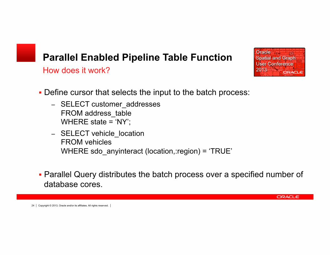
Define cursor that selects the input to the batch process: – SELECT customer_addresses
FROM address_table WHERE state = ‘NY’;
– SELECT vehicle_location FROM vehicles WHERE sdo_anyinteract (location,:region) = ‘TRUE’
Parallel Query distributes the batch process over a specified number of database cores.
How does it work?

Copyright © 2013, Oracle and/or its affiliates. All rights reserved. 25
Parallel Enabled Pipeline Table Function Exadata X2-2 ¼ RAC has 2 nodes, each with 12 cores (24 total)
ALTER SESSION FORCE PARALLEL DML PARALLEL 24; ALTER SESSION FORCE PARALLEL QUERY PARALLEL 24;
-- To balance parallel slaves across nodes. ALTER SESSION SET "_parallel_load_balancing"=false; CREATE TABLE results (id NUMBER, geom SDO_GEOMETRY);
INSERT /*+ append */ INTO results SELECT id, sdo_geometry (2001,8307,sdo_point_type(longitude,latitude,null),null,null) geom FROM TABLE( geocode_pipelined ( CURSOR(SELECT id, streetname, city, state, zip, housenum FROM ascii_addrs) )); COMMIT;

Copyright © 2013, Oracle and/or its affiliates. All rights reserved. 26
Parallel Enabled Pipeline Table Function Exadata X2-2 ¼ RAC has 2 nodes, each with 12 cores (24 total)
ALTER SESSION FORCE PARALLEL DML PARALLEL 48; ALTER SESSION FORCE PARALLEL QUERY PARALLEL 48; ALTER SESSION SET "_parallel_load_balancing"=true; (or don’t specify, true default)
CREATE TABLE results (id NUMBER, geom SDO_GEOMETRY);
INSERT /*+ append */ INTO results SELECT id, sdo_geometry (2001,8307,sdo_point_type(longitude,latitude,null),null,null) geom FROM TABLE( geocode_pipelined ( CURSOR(SELECT id, streetname, city, state, zip, housenum FROM ascii_addrs) )); COMMIT;

Copyright © 2013, Oracle and/or its affiliates. All rights reserved. 27
Parallel Pipelined Table Function
Exadata X2-2 ¼ RAC with 24 Cores
Batch geocoding – 1365/second Batch reverse geocoding – 3388/second Batch DEM get_cell_value raster lookups – 8951/second
Exadata Results

Copyright © 2013, Oracle and/or its affiliates. All rights reserved. 28
Hybrid Columnar Compression (HCC) and Spatial

Copyright © 2013, Oracle and/or its affiliates. All rights reserved. 29
HCC and Spatial
HCC is primarily for static or almost static data. Updates will uncompress compressed data (true for spatial and non-spatial data).
Point, Line and Polygon geometries can all benefit from HCC Lines and Polygons, they must be stored inline (less than 4K in size). Options include:
– COMPRESS FOR QUERY LOW – COMPRESS FOR QUERY HIGH – COMPRESS FOR ARCHIVE LOW – COMPRESS FOR ARCHIVE HIGH

Copyright © 2013, Oracle and/or its affiliates. All rights reserved. 30
HCC and Spatial
Two ways to compress: – Create Table As Select – Direct Path Inserts
1. Create Table As Select CREATE TABLE edges_compressed
COMPRESS FOR QUERY LOW NOLOGGING AS SELECT * FROM edges;

Copyright © 2013, Oracle and/or its affiliates. All rights reserved. 31
HCC and Spatial
2. Direct Path Inserts (full code example in presentation appendix)
-- PL/SQL Example with append_values hint. DECLARE id_tab ID_TAB_TYPE; edge_tab GEOM_TAB_TYPE; BEGIN -- Population of id_tab and edge_tab shown in presentation appendix FORALL i IN edge_tab.first .. edge_tab.last INSERT /*+ append_values */ INTO edge_ql VALUES (id_tab(i), edge_tab(i)); COMMIT;

Copyright © 2013, Oracle and/or its affiliates. All rights reserved. 32
HCC and Spatial – Uniform Geometries
Uniform geometries spatial layers have the same number of coordinates in every row.
Some examples: – Point data (x NUMBER, y NUMBER) – Box polygon (llx NUMBER, lly NUMBER, urx NUMBER, ury NUMBER) – Two point line (x1 NUMBER, y1 NUMBER, x2 NUMBER, y2 NUMBER) – Four point polygon (x1 NUMBER, y1 NUMBER, …, x5 NUMBER, y5
NUMBER)
For much higher compression rates, store uniform geometries as a series of NUMBER columns instead of SDO_GEOMETRY
Strategy For Much Higher Compression Rates

Copyright © 2013, Oracle and/or its affiliates. All rights reserved. 33
HCC and Spatial – “Uniform” Geometries
• Create a function based index on uniform geometries to perform spatial queries
• The following ANYINTERACT queries were run on a 116 million row table • Query High compression – 18.17x… queries still very fast.
Box Polygon With Function Based Index - Example
Anyinteract Query
Uncompressed Query Low 3.92x comp
Query High 18.17x comp
Archive High 21.57x comp
10 acre polygon
(487739 rows returned)
1.86 sec 2.02 sec
(1.08x perf)
2.7 sec
(1.45x perf)
12.75 sec
(6.85x perf)

Copyright © 2013, Oracle and/or its affiliates. All rights reserved. 34
HCC and Spatial – “Uniform” Geometries
SDO_Within_Distance queries against compressed “uniform” geometries
Box Polygon With Function Based Index - Example
Within_Distance Query
Uncompressed Query Low 3.92x comp
Query High 18.17x comp
Archive High 21.57x comp
0.1 mile
(1096 rows)
0.10 sec 0.12 sec
(1.2x perf)
0.24 sec
(2.4x perf)
1.63 sec
(16.3x perf)
0.5 mile
(25996 rows)
0.84 sec 1.17 sec
(1.39x perf)
2.98 sec
(3.54x perf)
24.34 sec
(28.97x perf)
1 mile
(103226 rows)
3.00 sec 4.26 sec
(1.42x perf)
10.83 sec
(3.61x perf)
88.30 sec
(29.43x perf)

Copyright © 2013, Oracle and/or its affiliates. All rights reserved. 35
SELECT count(*) FROM businesses WHERE SDO_ANYINTERACT (geometry, sdo_geom.sdo_buffer(sdo_geometry(2001,8307, sdo_point_type (-122.3, 37.7,null), null, null), 4, 0.05, 'unit=mile')) = 'TRUE‘;
SDO_ANYINTERACT + SDO_BUFFER vs SDO_WITHIN_DISTANCE
Not conclusive… sdo_anyinteract with sdo_buffer () as query window may be faster than sdo_within_distance.
Still under investigation…. May be worth a try.

Copyright © 2013, Oracle and/or its affiliates. All rights reserved. 36
HCC – Non Uniform Geometries
Non-uniform geometries layers can have a different number of coordinates in every row.
Some examples: – Zip code polygons – County polygons – Road line strings
Use SDO_GEOMETRY for non-uniform geometry columns

Copyright © 2013, Oracle and/or its affiliates. All rights reserved. 37
HCC and Spatial (SDO_GEOMETRY)
• Point data is uniform, storing it as two Oracle NUMBERs (instead of SDO_GEOMETRY) can achieve much better compression rates than the ones below.
• See compression rates for uniform data on previous slides.
Point data
Within_distance Query
Uncompressed Query Low 3.5x comp
Query High 5.3x comp
Archive High 6.8x comp
4 mile
(323 rows)
0.02 sec 0.02 sec
(0.0x perf)
0.06 sec
(3.0x perf)
1.36 sec
(68x perf)
5 mile
(1251 rows)
0.03 sec 0.06 sec
(2.0x perf)
0.12 sec
(4.0x perf)
2.77 sec
(92x perf)
10 mile
(31466 rows)
0.29 sec 0.61 sec
(2.1x perf)
1.3 sec
(4.5x perf)
32.11 sec
(110x perf)

Copyright © 2013, Oracle and/or its affiliates. All rights reserved. 38
HCC and Spatial (SDO_GEOMETRY) Line / Polygon data
Within_distance Query (lines)
Uncompressed Query Low 3.5x comp
Query High 5.3x comp
4 mile
(809 rows)
0.08 sec 0.18 sec
(2.25x perf)
0.48 sec
(6x perf)
5 mile
(3079 rows)
0.16 sec 0.38 sec
(2.375x perf)
0.99 sec
(6.188x perf)
10 mile
(80771 rows)
1.75 sec 3.91 sec
(2.23x perf)
10.34 sec
(5.91x perf)
• SDO_ANYINTERACT with SDO_BUFFER query window could produce faster response times.... May want to give it a try.

Copyright © 2013, Oracle and/or its affiliates. All rights reserved. 39
HCC and INSERT /*+ append_values */
Currently, INSERT /*+ append_values */ can HCC compress points, lines and polygons
Lines and Polygons must be less than 4K (stored inline) INSERT /*+ append_values */ does not compress if the column
contains a spatial index. – The lifting of this restriction is under investigation.

Copyright © 2013, Oracle and/or its affiliates. All rights reserved. 40
Massive Spatial Ingests
Copyright © 2013, Oracle and/or its affiliates. All rights reserved. 41
Massive Spatial Data Ingest
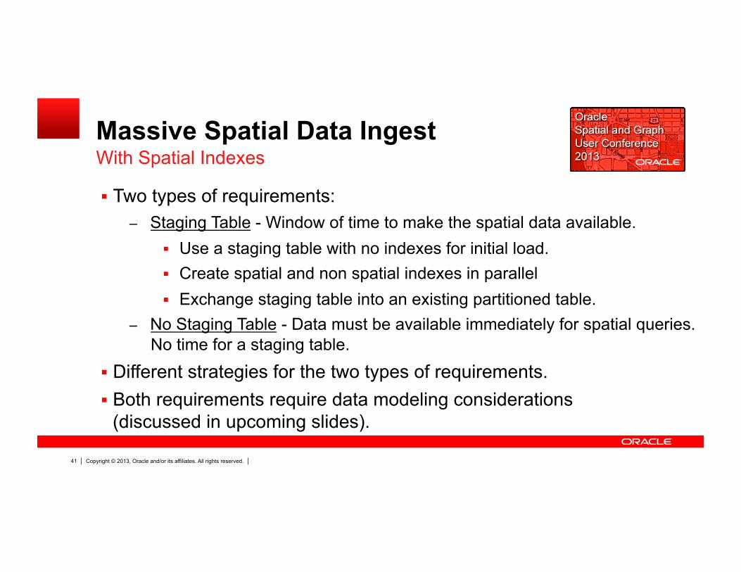
Two types of requirements: – Staging Table - Window of time to make the spatial data available.
Use a staging table with no indexes for initial load. Create spatial and non spatial indexes in parallel Exchange staging table into an existing partitioned table.
– No Staging Table - Data must be available immediately for spatial queries. No time for a staging table.
Different strategies for the two types of requirements. Both requirements require data modeling considerations
(discussed in upcoming slides).
With Spatial Indexes

Copyright © 2013, Oracle and/or its affiliates. All rights reserved. 42
Massive Spatial Ingests With A Staging Table

Copyright © 2013, Oracle and/or its affiliates. All rights reserved. 43
Massive Spatial Data Ingest
Major benefits are performance and manageability of very large data sets
Customer example: – Requirement:
Ingest and maintain 2 days of weather data online 270,000 samples every 30 seconds (Oracle Spatial can do even
more…) – Implemented with:
30 second partitions (5760 partitions over 2 days) New partitions rolled on, older partitions rolled off
With A Staging Table

Copyright © 2013, Oracle and/or its affiliates. All rights reserved. 44
Massive Spatial Data Ingest
Load data into a staging table with no indexes (called new_weather_data) Parallel create index (spatial index too) on staging table Partition P1 is an empty leading partition Update partitioned table with new weather data in a fraction of a second. No need to maintain an index on INSERT !!!!
With A Staging Table
ALTER TABLE weather_data_part EXCHANGE PARTITION p1 WITH TABLE new_weather_data INCLUDING INDEXES WITHOUT VALIDATION;

Copyright © 2013, Oracle and/or its affiliates. All rights reserved. 45
Massive Spatial Ingests Without A Staging Table

Copyright © 2013, Oracle and/or its affiliates. All rights reserved. 46
Massive Spatial Data Ingest
Spatial data must be inserted and committed immediately No time for a staging table. If possible, don’t commit after every insert. If possible, perform batch inserts. Set sdo_dml_batch_size=15000 when you create the spatial index.
– PL/SQL - FORALL BULK INSERTS (example in appendix) – Java - JDBC UPDATE BATCHING – C – Array inserts
Without A Staging Table

Copyright © 2013, Oracle and/or its affiliates. All rights reserved. 47
Massive Spatial Data Ingest
Very Common Misconception:
"Increasing number of connections in a pool and number of threads performing inserts will increase spatial data insert
throughput”
– Only true if no connections in pool write to the same spatial index. – For high ingest rates, even two connections writing to the same spatial
index can adversely affect spatial index ingest performance.
Without A Staging Table (continued)

Copyright © 2013, Oracle and/or its affiliates. All rights reserved. 48
Massive Spatial Data Ingest
Quick fix… try streaming all writes to one connection in the pool. – One connection for writes – Many connections for reads
To really maximize spatial ingest throughput: – Use multiple connections in a connection pool – Dedicate each connection to one spatial index. – This eliminates all spatial index contention.
Strategy continued on next slide.
Without A Staging Table (continued)

Copyright © 2013, Oracle and/or its affiliates. All rights reserved. 49
Massive Spatial Data Ingest
• Example is hourly, but could be monthly or quarterly • Multiple threads perform batch inserts, each with a dedicated process id CREATE TABLE composite_example ( t timestamp , process_id number , geom sdo_geometry , hour_partition as (substr(t,1,12))) PARTITION BY RANGE ( hour_partition, process_id ) (PARTITION DAY1_H5_1 VALUES LESS THAN ('30-NOV-10 05', 2 ), PARTITION DAY1_H5_2 VALUES LESS THAN ('30-NOV-10 05', 3 ), PARTITION DAY1_H5_3 VALUES LESS THAN ('30-NOV-10 05', 4 ), PARTITION DAY1_H6_1 VALUES LESS THAN ('30-NOV-10 06', 2 ), PARTITION DAY1_H6_2 VALUES LESS THAN ('30-NOV-10 06', 3 ), PARTITION DAY1_H6_3 VALUES LESS THAN ('30-NOV-10 06', 4 ), PARTITION REST VALUES LESS THAN (MAXVALUE,MAXVALUE));

Copyright © 2013, Oracle and/or its affiliates. All rights reserved. 50
Massive Spatial Data Ingest
Inserts per second with spatial index enabled – Parallel Degree - how many threads performing bulk inserts in parallel – For 1 million row partition, 15K batches, 66,123.57 inserts per second
X2-2 Quarter RAC Exadata - Results

Copyright © 2013, Oracle and/or its affiliates. All rights reserved. 51
Massive Spatial Data Ingest X2-2 Quarter RAC Exadata - Results
0 10,000 20,000 30,000 40,000 50,000 60,000 70,000 80,000 90,000
1 2 8 12 8x2 12x2
(100k/15k)
(1m/15k)
Number Of Cores
Inserts Per Second

Copyright © 2013, Oracle and/or its affiliates. All rights reserved. 52 52
Q&A

Copyright © 2013, Oracle and/or its affiliates. All rights reserved. 53
May 22, 2013 Ronald Reagan Building and International Trade Center
Washington, DC USA