11) if I127/ _

Analytical Method for Turbine Blade Temperature Mapping‘ to Estimate a Pyrometer Input Signal

byJames D. MacKay

Thesis submitted to the Faculty of the

W Virginia Polytechnic Institute and State University

W in partial fuliillment of the requirements for the degree of

Master of Sciencein

Mechanical Engineering

' APPROVED:

Walter F. O’Brien, Chairmanl

Hal L. Moses Henry L. Wood

1I11May 1987 l

Blacksburg, Virginia II

111I

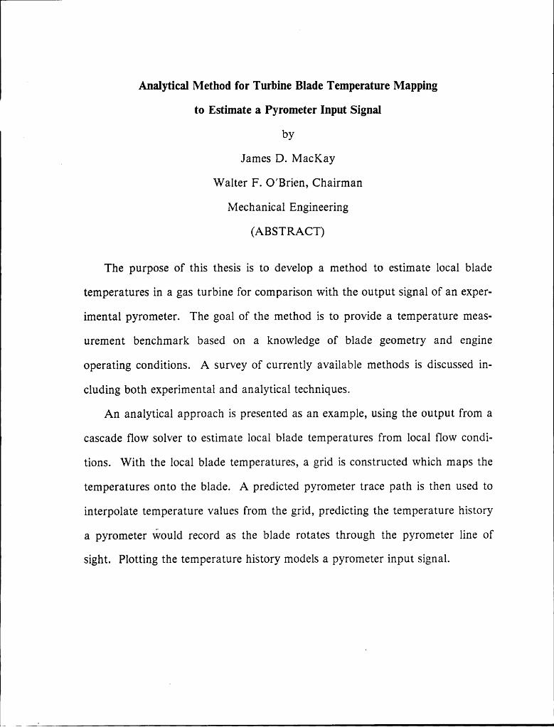
Analytical Method for Turbine Blade Temperature Mapping

to Estimate a Pyrometer Input Signal

aß byy James D. MacKay

Walter F. O’Brien, Chairman

Mechanical Engineering

(ABSTRACT)

The purpose of this thesis is to develop a method to estimate local blade

temperatures in a gas turbine for comparison with the output signal of an exper-

imental pyrometer. The goal of the method is to provide a temperature meas-

urement benchmark based on a knowledge of blade geometry and engine

operating conditions. A survey of currently available methods is discussed in-

cluding both experimental and analytical techniques.

An analytical approach is presented as an example, using the output from a

cascade flow solver to estimate local blade temperatures from local flow condi-

tions. With the local blade temperatures, a grid is constructed which maps the

temperatures onto the blade. A predicted pyrometer trace path is then used to

interpolate temperature values from the grid, predicting the temperature history

a pyrometer would record as the blade rotates through the pyrometer line of

sight. Plotting the temperature history models a pyrometer input signal.

I

Acknowledgements

I would like to express my deepest gratitude to my advisor and friend Dr.

Walter F. O’Brien. I have learned a great deal associating with him and have

had fun times.

Thanks also to my teachers and committee members, Dr. Henry Wood and

Dr. Hal Moses. Dr. Wood’s office is the best learning spot in Randolph, I hope

I didn’t take up to much of his time there.

Of course, Rosemount Aerospace made the project possible and I am grateful

for their sponsorship and help.

l

Acknowledgements an I

i

Table of ContentsL

Introduction ............................................................ l

Literature Review ........................................................ 5

Aerothermodynamic Approach ............................................... 8

Current Research Program ................................................ I2

Example Procedure - Initial work ............................................ I6

Flow Solver Output Processing ............................................. 22

Estimating Blade Temperature .............................................. 36

Conclusions ........................................................... 62

Table of Contents iv

I

·iFuture Work Recommendations ............................................. 64 (I

IReferences ............................................................ 67 ;I11

vera ................................................................. 70 }I

1I

II

Table of Contents v

2

List of Illustrations

9 Figure 1. JT15D-1 Cross section schematic ....................... 14

Figure 2. Pyrometer penetration ............................... 15

Figure 3. Grid for section A-A (6% blade height) .................. 23

Figure 4. Grid for section B-B (28% blade height) ................. 24

Figure 5. Grid for section C-C (49% blade height) ................. 25

Figure 6. Grid for section D-D (92% blade height) ................. 26

Figure 7. Mach number vector field plot for section A-A (6% height) . . . 27

Figure 8. Mach number vector field plot for section B-B (28% height) . . .28

· Figure 9. Mach number vector ficld plot for section C-C (49% height) . . 29

Figure 10. Mach number vector field plot for section D-D (92% height) . . 30

Figure 11. Mach number vs. percent axial chord for section D-D streamlines 32

Figure 12. Mach number vs. percent axial chord for section D-D streamlines 33

Figure 13. Tr_ailing edge grid lines for section D-D . . .'............... 39

Figure 14. Corrected Mach number and Temperature profiles ......... 42

Figure 15. Corrected Mach number and Temperature profiles ......... 43

Figure 16. Model pyrometer trace path curve and available cross sections . 45

Figure 17. Model pyrometer input signal at design (95% speed) ........ 46

List of ulustistions vi

Figure 18. Off·design Mach number vector plot for section A-A (85% speed) 52 IFigure 19. Off-design Mach number vector plot for section B·B (85% speed)53Figure20. Off-design Mach number vector plot for section C-C (85% speed) 54 E

_ Figure 21. Off-design Mach number vector plot for section D-D (85% speed)55Figure22. Off-design Mach number vs. percent axial chord for D-D .... 56 I

Figure 23. Off-design Mach number vs. percent axial chord for D-D .... 57Figure 24. Off-design corrected Mach number and Temperature profiles . . 58Figure 25. Off-design corrected Mach number and Temperature profiles . . 59Figure 26. Model pyrometer input signal for of“f·design (85% speed) ..... 60Figure 27. Relative emissive power comparison between 85% and 95% speed 61

»E

List ofillusmcions vii I

E

Nomenclature

A, cascade inlet area

A2 cascade exit area

oz, inlet Velocity angle

a2 exit Velocity angle

B2 exit blade angle

c flow rate constantcp specific heat

y ratio of specific heats

k stage work constant

M - Mach numberm mass flow rateM, inlet Mach number

M2 exit Mach number EN percent maximum wheel speed 1

äNomenclature visa E

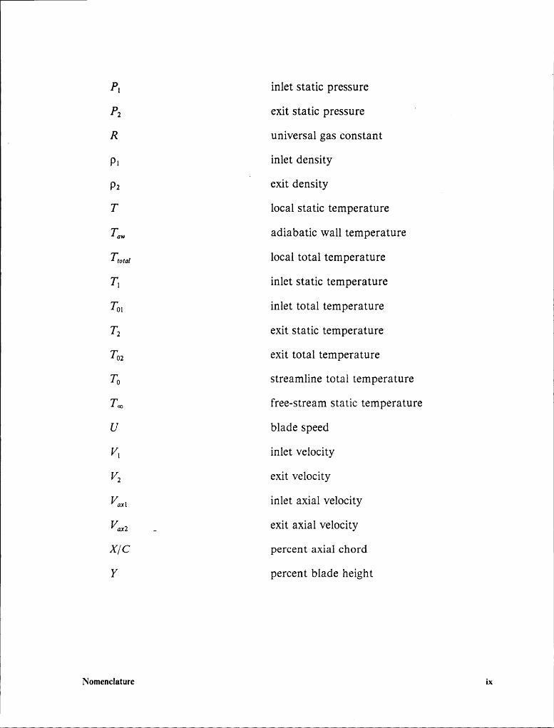
IP, inlet static pressure

l

P2 exit static pressure ‘

_ R universal gas constant

p, inlet densityp2 exit density

T local static temperatureT„„ adiabatic wall temperature

Kom, local total temperature

T, inlet static temperature

TO, inlet total temperature

T2 exit static temperature

T,,2 exit total temperature

To streamline total temperatureT,„ free-stream static temperature

U blade speedV, inlet Velocity

V2 exit Velocity

VM, inlet axial Velocity

VM, _ exit axial Velocity

X/C percent axial chord

Y percent blade height

Nomenclature ix P

II

II

Introduction I

The benefits that radiation pyrometers can provide for gas turbine operation

forecast their use as an integral part of many engines in the future. The primary

benefit of a pyrometer for monitoring turbine blade temperatures is that it is a

non-contacting, accurate feedback for fuel control systems, providing immediate

performance improvements by allowing a given turbine to operate closer to its

potential. Pyrometers can be used for condition monitoring as well. For example,

the information gained can be used for better prediction of the need for hot-

section overhauls. Pyrometers can also be used to detect abnormally hot blades,

perhaps caused by blocked cooling passages, in time to prevent an actual failure.

Measuring blade temperature directly is an additional advantage, especially in

an era of cooled turbine blading.

There is a current need to adapt experimental pyrometers to production en-

gines and to prove their performance and reliability. This thesis work is part of 1

a pyrometer research program by the Center for Turbomachinery and Propulsion ÄI

Introductionl

1 II

Research at Virginia Tech, supported by the Rosemount Aerospace Division.i

'Durability and lens optics cleansing are primary development areas being inves-

tigated. The key to the acceptance of the pyrometer, however, is in proving the

accuracy of its temperature measurement. The focus of this paper is the tem-

perature accuracy issue.

The current need is to provide a benchmark for local blade temperature. ToT

prove the accuracy of the pyrometer it is essential to have an alternative temper-

ature indicating technique for comparison with the pyrometer-measured temper-

ature signal. Pyrometer input signals for an operating gas turbine must be

determined to evaluate pyrometer performance such as accuracy, response time,

and precision.

The ideal comparison model would be an accurate map of the turbine blade

temperature at a given operating condition. The temperature at any given point

on the blade, in coordinates of percent axial chord vs. percent blade height pro-’ vides the basis for modeling an input signal. A geometric analysis, albeit a com-

plex one, could determine the line (or swath) the pyrometer focus spot traces

across the blade as the blade rotates through the line of sight of the detector.

Transforming the trace path into coordinates of percent axial chord and percent

blade height, and then plotting the corresponding blade temperatures would

provide an excellent input signal model.

The extremely harsh environment of the turbine rotor, with its high temper-

atures, corrosive gases and severe centrifugal stresses, makes measurement of the

local blade temperature difficult. There are several methods of temperature in- II

Introduction 2

dication available today, including intermediate turbine temperature (ITT) gages,A

thermal paints and thermocouples. These methods may help evaluate pyrometer

performance, but each has its shortcomings.2 An ITT gage allows engine operators to watch for hot starts and to judge

optimum throttle position. A typical gage derives ITT by using an analog

thermocouple circuit to add three times the temperature rise across the fan to the

exhaust gas temperature (EGT), based on the assumption that the temperature

drop through the two low pressure turbine stages is approximately three times the

fan temperature rise (for a 3 to l bypass ratio engine) [I]. The ITT gage, though

relatively inaccurate, is a good general indicator of the temperature conditions

within the turbine and provides an ample safety margin in a relatively simple, low

cost manner. However, this method estimates average gas temperature, rather

than blade temperature, and thus is of limited use in estimating blade temper-

atures.

An engine may be satisfactorily operated with this type of gage, but for

pyrometer development it is only a general indicator of turbine temperature.

Unfortunately, it cannot be used to directly estimate the temperature distributionH on a turbine blade.

l

Thermal paints indicate blade temperature directly, but are limited in appli-

cation. The paints change either color or luster at a certain temperature. Avail-

able paints are limited to I4 to 28 degree (C) increments and can only be checked

in post-run inspections. It is planned to use thermal paints as an additional

check, but they are impractical for real time measurement.

Introduction . 3

1

Imbedding thermocouples into turbine blades is another alternative whichJ

others have tried for research and development purposes [2]. This approach is

practical in wind tunnel test rigs, but poses several difüculties in an actual gas

turbine installation. Instrumented blades are costly to produce and compromised

in strength. Their questionable reliability is a problem due to the additional ex-

pense incurred when their replacement requires a hot section tear-down.

Thermocouples are also sensitive to conduction problems as they are composed

of materials different from those of the turbine blades [2]. Furthermore, the slip

ring system for transmitting thermocouple voltage from the rotor to the controller

poses severe problems owing to the high wheel velocities in many turbines. This

latter problem may be eliminated with further development of the Fiber Optic

Rotating Joint [3], however this may also prove costly and fragile.

Conventional measurement techniques are currently incapable of providing

a reasonable comparison for a pyrometer in an actual engine. Thus an analytical

approach seems to be a most promising avenue along which to pursue turbine

blade temperature research.

With cascade flow solvers becoming readily available (see Literature Review)

[4,5], it is logical to take an aerothermodynamic approach to estimate local blade

temperature from local flow conditions. The following section outlines the

aerothermodynamic procedure, and subsequent sections describe an example lprocedure applied to a current research project. j

rnttoonotaon 4

Literature Review

The literature supporting this work comes from several branches of gas tur-

bine research. Papers concerning radiation pyrometry, turbine blade heat trans-

fer, and cascade flow solvers all helped focus and support this work.

The early pyrometer papers focused on the theory behind pyrometer appli-

cations, possible benefits, and early designs for gas turbine pyrometers. Barber’s

paper of 1969 is one of the best of the early papers. Radiation theory, design

requirements and early problems are all covered. Especially noteworthy is the

fact that radiative energy emitted by a body ideally varies by the fourth power

of temperature, hence the accuracy potential of the radiation pyrometer is high

indeed. Initial pyrometers were strictly analog systems, fuel cooled, and designed

to measure average blade temperature for the entire disk [6].

Advances in pyrometer systems in the seventies were dramatic. The fre-L quency response of detector systems increased to the point where rough individ-

ual blade temperature profiles could be monitored. The introduction of dual1

Literature Review S [11

1

spectrum pyrometers allowed emissivity and reflection effects to be accounted for

in signal processing circuits. Atkinson and Strange present the radiation theory

behind dual spectrum pyrometry and confirm the theory with experimental data

in their report [7]. With modern tiltering systems, hot particle flashes could be

rejected. ln addition, über optics allowed the silicon transducer to beremovedfrom

the hot section area and eliminated the need for external cooling systems.

Frequency response and necessary signal processing techniques for a detection

system based on considerations of optical efticiency, spatial resolution , temporal

resolution, and temperature range are detailed in the extensive work of Douglas

[8]. Benyon’s paper neatly summarizes the ’ground rules’ for a pyrometer system

design and installation for use by new and prospective users of turbine pyrometry

[9]. The radiation pyrometer has been proven under laboratory conditions, but

the need for further development and testing of advanced systems for in-flight

use in actual engines is apparent.

Most turbine blade heat transfer work is concentrated on cooled blades. Se-

veral heat transfer papers were useful in confirming the adiabatic wall assump-

tion and for suggesting future improvement areas. These papers are referenced

in the text where used.

A look at cascade flow solver literature is valuable for comparing the output

of the available solver to results for similar geometries in published material.

Holmes and Tong apply their solver to turbine blades and present results and

comparisons to experimental data that are similar to the results obtained in the

present work [5]. A paper presented by Denton and others also presents relevant

Literature Reviewl

6

results (both experimental and computational) and discusses the nature of turbine·passage shocks [10]. The results of these papers helped give confidence in the

flow solver output of this project.

The reviewed material is just a small sample of the flow solvers available to-

day. The abundance of computational flow solvers are an indication that the

solvers necessary to carry out the following temperature indication scheme are

readily available. Other computational fluids papers highlighted problems withthe trailing edge flow and outlined solution techniques that were adopted for this

work. These are also referenced as they are used in the text.

ILiterature Review 7

Aerothermodynamic Approach

The Literature Review contains references to several examples of the cascade

solvers currently available. The codes available today are capable of handling

transonic two-dimensional flows with a good degree of accuracy and relatively

short computer run times. A typical cascade solver takes geometric boundary

conditions and inlet aerothermodynamic data (inlet velocities, temperatures, and

flow angles) and solves for the velocity distribution within the cascade. Some

solvers also need exit conditions to obtain the interior solution. The velocity field

can then be used to estimate wall temperature.T All solvers require blade geometry as input. By breaking the two-dimensional

channel that models the rotor into a reasonable number of finite areas for nu-

merical analysis, smoothness is sacrificed to keep run times reasonable. A turbine

airfoil broken into fifty axial points per surface limits accurate modeling of lead-

ing and trailing edge details, but provides an overall velocity distribution with

acceptable accuracy. Blade geometry must be given by themanufacturers,Aerothermodynamic

Approach 8 D

1

measured from an example blade, or estimated in some manner. Of course, a

knowledge of the blade shapes is also essential to calculate the pyrometer trace

path.p

Any geometry available must be rotated into a coordinate system compatible

with the solver code used. The same must also be done with aerothermodynamic

boundary conditions.

Matching cascade solver results to conditions within the actual gas turbine1

poses an additional problem. Possessing cycle data for the engine for a variety

of operating points alleviates much of the problem. With this data it is only

necessary to determine the operating point of the actual test engine, and to cor-

rect for current ambient conditions. Otherwise, several assumptions must be

made. Given design conditions, off-design conditions must be either calculated

from a cycle analysis or estimated based on information from conventional engine

instrumentation and several assumptions. The assumptions of constant gas an-

gles for the turbine inlet nozzles and constant relative exit angles for the rotor,

allow the off-design stage temperature ratio to be calculated using an analytical

method [1 l]. This method and experimental data are combined to carry out an

iterative proce-dure that satisfies the velocity triangle constraints, the conditions

of continuity, and the choked turbine non·dimensional flow rate. The details of

this procedure are discussed in a following section presenting off-design work.

Accurate passage flow modeling must include the variations in flow condi- 1tions from blade root to tip. This information may also be provided, or it can1

Acrorhcrrrrodyharhac Approach 9

be estimated using a free-vortex rotor design assumption to calculate the radial

distribution of aerodynamic boundary conditions from given mid-passage data.

. Once the boundary conditions are decided and velocity solutions are com-

puted, a local wall temperature distribution can be derived from the velocity field.

The preferred method would be an interactive boundary layer solution that

produced wall temperature directly, based on an assumed wall heat flux bound-

ary condition. Most available codes are still inviscid solvers, thus a temperature

recovery scheme is a logical approach to the problem. The simplest method is the

adiabatic wall recovery relation with a constant recovery factor.

Calculating the local blade temperatures based on the local flow variables for

each of the cross sections leads to a set of surface blade temperature profiles lay-

ing on the blade axially at various heights corresponding to the cross sections fed

into the flow solver. Transforming the cross section blade heights into non-

dimensional coordinates of percent blade height, and also, the axial temperature

points into percent axial chord, creates a temperature grid that maps onto the

blade surface.

A geometric analysis on a computer-aided design (CAD) system can deter-

mine the coordinates of the pyrometer trace path in the same system of percent

blade height and percent axial chord, The calculated intersection coordinates can

then be used as the input to interpolate for the temperatures the pyrometerA

would see during a blade passage.

Aerothermodynamic Approach l0

I

The pyrometer line-of-sight coordinates in terms of time can call blade tem-

peratures from the grid map to indicate pyrometer temperature input vs. time for

a given operating condition.

The following chapters briefly describe the pyrometer project and outline the

aerothermodynamic procedure used for the project. Some of the problems en-

countered may be unique to this project, but the application of the procedure

demonstrates the feasibility, merit, and limitations of the method, while at the

same time showing the theory and modeling necessary to carry out the entire

procedure.

lI

Acrothermodynamic Approach ll I

1

Current Research Program

Pyrometer development for gas turbine applications has progressed to the

point where testing in actual engines is now essential (see Literature Review).

The Center for Turbomachinery and Propulsion Research at Virginia Tech is

currently involved in a pyrometer installation research project. The project en-

tails installing a pyrometer in a gas turbine and extensively testing and developing

1 the pyrometer system for future use as a control feedback element.

The Pratt & Whitney JTl5D-lA turbofan currently occupying the Virginia

Tech Airport test cell serves as an excellent pyrometer test bed, in part because

its uncooled first stage turbine lends is well-suited to analytical temperature esti-

mates. If the pyrometer proves accurate on the uncooled blades, it can then be

confidently applied to cooled blades.

The JTl5D is a small 2000 lb. thrust class, 3.3 bypass ratio, twinspool engine

commonly installed in tandem on the Cessna Citation or Aerospatiale Corvette

business jets [1]. The first stage turbine of this engine has seventy-one blades and

Current Research Program 12

a design speed of over 30,000 rpm [12]. An engine cross section schematic isI]

shown in Figure 1, and the pyrometer penetration in Figure 2. Unfortunately,

the folded burner adds complexity to the installation, and limits direct viewing to‘ only the suction side of passing blades. The line of sight intersects the blade pri-

marily in the mid-section to tip region and is blind to the leading edge. Parallel

CAD work is being performed using wireframe surface modeling to determine the

exact path the pyrometer sight beam inscribes.

In the adjacent control room, an IBM PC-based data acquisition system

supports a conventional aircraft cockpit display of engine operating information.

Information logged, such as inlet total temperature and pressure, high and low

spool percent speed, compressor discharge pressure, ITT, and fuel flow rate will

serve as inputs to locate the engine operating point. The operating point will in

turn determine the input to the cascade solver, ultimately leading to a model

pyrometer signal. Operating in parallel is an IBM PC AT linked to a LeCroy

high—speed analog-to-digital converter dedicated to handling the pyrometer out-

put.

The blade temperature calculation method presented supports the project and

is related to data gathered at the facility. The method is unique to the the JTISD

project in several ways, but illustrates an example of the aerothermodynamic ap-

proach outlined previously and provides example results.

l

,Current Research Program I3 5

i II l

I {A I

I

*L——L„„ ·

IV IIII Q I . _;AA ‘~ A ,, —~ AAAI

*«° '» I I *~„ ä1* Q “‘ P‘,

;j__‘ fy Q‘ · A in

_,.I A AAi_ AA .}*1__--:1I W

__ ,\ Ä‘ __

„/A/Af A

;—•- ‘~

- I!,' r— A\ ; Q L" _

° E I A I—· FA Ai. I I = I I ’ Q _;Ag ”"

&%‘~ 1 '° -. ‘

"‘A”AA AAZ: __l:,

II

Current Research Program I4 :

I

'II

; .. Ü II„‘?; {Y ·

‘„ _„ Ö II \III I ··· I® I

CII I ÄII ··I

I ‘ _

I

III III

I(I I,

I U" I— <I

Currcnt Rcscarch Program II5 I

Example Procedure - Initial work l

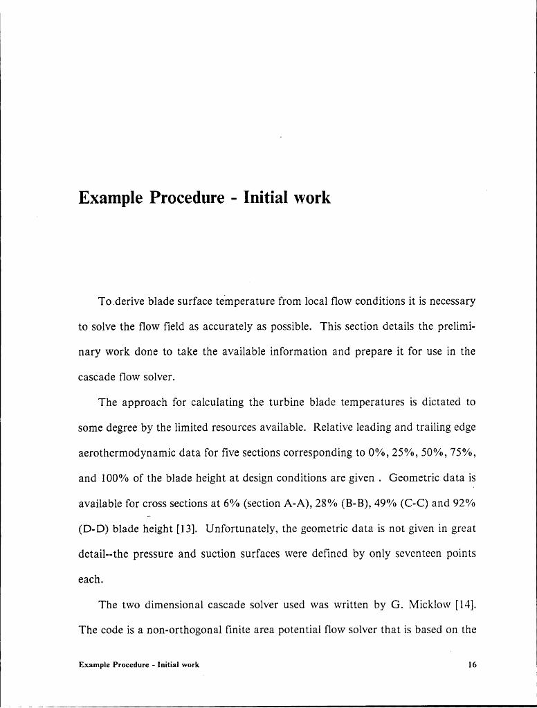
To .derive blade surface temperature from local flow conditions it is necessary

to solve the flow field as accurately as possible. This section details the prelimi-

nary work done to take the available information and prepare it for use in the

cascade flow solver.

The approach for calculating the turbine blade temperatures is dictated to

some degree by the limited resources available. Relative leading and trailing edge

aerothermodynamic data for five sections corresponding to 0%, 25%, 50%, 75%,

and 100% of the blade height at design conditions are given . Geometric data is

available for cross sections at 6% (section A-A), 28% (B-B), 49% (C-C) and 92%

(D-D) blade height [13]. Unfortunately, the geometric data is not given in great

detail--the pressure and suction surfaces were defined by only seventeen points

each.

The two dimensional cascade solver used was written by G. l\/Iicklow [14].

The code is a non-orthogonal finite area potential flow solver that is based on the

Example Procedure - Initial workl

16

I

integral continuity equation for compressible, isentropic flow. The inviscid code‘ is a portion of in his work that will later mesh with a boundary layer code and

an unsteady flow code. Though originally conceived to handle slightly transonic

compressor cascades, the code was modified to include the mildly supersonic

turbine case. Micklow, by referring to the research done for this thesis, was able

to to stretch and confirm the range of applicability of his solver. Micklow’s code

has been confirmed on several geometries given in a paper by Caspar [15].

Micklow also certifies, based on a review of the results, that the solutions are ac-

curate, subject to the inviscid isentropic assumptions and the limited geometric

data available.

The next step in the procedure was to model a turbine blade using the

thirty-four points given. The original attempt involved the use of a simple cubic

spline. However, this method distorted the trailing edges of the blades abnor-

mally. Instead, a parametric spline combined with a judiciously placed circle_for‘ the trailing edge radius is used to generate additional points. The low number

of points given effectively limits the justifiable number of additional points that

may be accurately added by interpolation. Using a finer mesh may lead to a

perceived increase in accuracy of the solution; however, the results would be

based on geometric boundary conditions that are not necessarily more accurate.

This fact, coupled with the desire to keep the computer run times reasonable,

leads to a practical ceiling of fifty axial points per surface.

As a result of the limited number of axial points, modeling rounded trailing

edges is impossible, and cusps must be used to cap slightly lengthened blades.

Example Pmeellme - Initial week l7

Each cusp is located such that the average of the upper and lower slopes nearly

matches the trailing edge velocity angle. This method was successfully used in the

work of Essers and Kafyeke [16]. Another major criterion for generating smooth’ blades is to keep slopes monotonically increasing up to the blade surface peak and

monotonically decreasing from the peak to the trailing edge point. This condition

helps eliminate a wavy surface boundary line that often leads to instability.

Since two of the typically five or seven streamlines between a blade row are

the pressure and suction surfaces of adjacent blades, any abrupt changes in the

geometry of these surfaces will have important effects. Sharp changes in surface

slopes can lead to numerical instability, because of the induced rapid changes in

the local flow variables. As a result, acceptable local convergence can be impos-

sible and global convergence both difficult and costly. Future programs, not

ready in time for this work, will include the boundary layers developed as

streamlines, making the inviscid code less sensitive to blade geometry.

Geometrie difficulties center at the leading and trailing edge regions where

blade slopes vary rapidly. These changes in slopes cause the grid generator to

form overlapping polygons which lead to' negative areas and adversely affect

convergence. -Leading edge effects need be minimized only to help global con-

vergence; the leading edge cannot be seen by the pyrometer. Simply increasing

the number of axial points to the practical maximum of fifty best achieves this

result. For the trailing edge, convergence is assured by making painstakingly

I certain that the slopes in the region are strictly monotonic and that the changes

;Example Procedure - Initial work l8

1 1in slope are averaged over several points. This procedure is roughly equivalent

to making the second derivative of the surface line smooth.

Once the blade smoothness is satisfactory, it is necessary to match the given

geometric cross sections to the available aerodynamic data. Because the blades

were designed using a free vortex condition, with a nearly constant relative trail-

ing edge angle, interpolation of proper aerothermodynamic data for the geometric

sections introduces little, if any, error. To mesh with the grid generator of the

cascade solver it is necessary to rotate all the aerodynamic data and geometry to

the proper stagger angle for each geometric cross section.

The aerodynamic data given by the engine manufacturer was computed as-

suming constant relative total temperature along streamlines through the rotor,

which does not conflict with the assumptions of Micklow’s code. However, a

problem that has to be addressed is the conflict between using an inviscid

isentropic code and being given cycle-generated aerothermodynamic data that

empirically includes total pressure losses and some underturning.

The solution is to use the known upstream conditions and generate isentropic

exit conditions. The energy equation, the continuity equation, and the ideal gas

equation of state can bc solved for the three unknown exit conditions, given the

upstream Mach number, temperature, and velocity angle. These equations do

not yield a closed form solution, but rather are used to generate a table for exit

velocity angle and temperature based on an assumed exit Mach number.

Starting with the continuity equation:

pl!/ax1A1 = p2Vax2/12 ($1)

Example Procedure - Initial work 19

I 1

The annular entrance area Al equals the annular exit area A2 for the rotor, and

velocity angles can be introduced to obtain:1

pl Vl cos ol = p2 V2 cos (12 (3.2)

Introducing the ideal gas equation of state to solve for p and the definition of

Mach number leads to:

P ;- P __cos oil cos 012 (3.3)

cancelling and grouping,

cosot = os01 (3 4)2 P2 M2 1

....P. T. ä .then using the isentropic relation 73- = yieldszI l

Y

cos (12 cos dl (3.5)M2 T2

Assuming M2,-the energy equation (T,o,„,= constant) can be solved for Tl and T2

using the relation:

TT = (3.6)1 + —M22 I

II

Example Procedure - Initial work 20 1

Substituting Eq. (3.6) into Eq. (3.5) allows a table based on assumed M2 tobe created. The table consists of a list of M2 values and the corresponding

isentropic exit velocity angles and exit local gas temperatures. The most logical

choice is the solution with the exit Mach number that matches the given design

exit Mach number. As would be expected, the turning angle is a degree or so

greater for the isentropic case, but the cascade solver has better convergence usingi

these values. In initial work, the flow modeled was trying to turn in the wake to

match downstream conditions.

At this point all preliminary work to run the cascade solver is complete. The

blade smoothing procedure and isentropic exit condition calculations are per-

formed for each of the four geometric cross sections. The next section describes

the use of the output of the cascade solver and the initial processing of the output

data.

1

lExample Procedure - Initial werk 2l 1· 111

1° 1

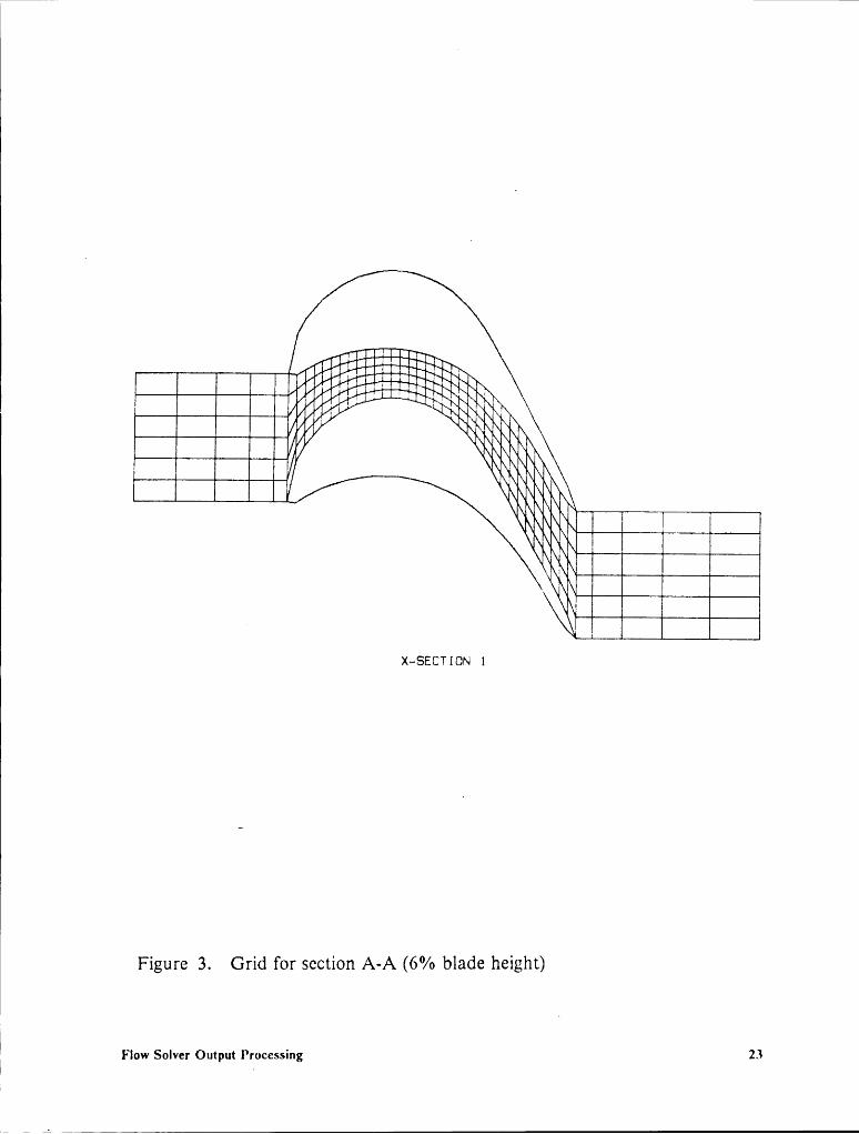
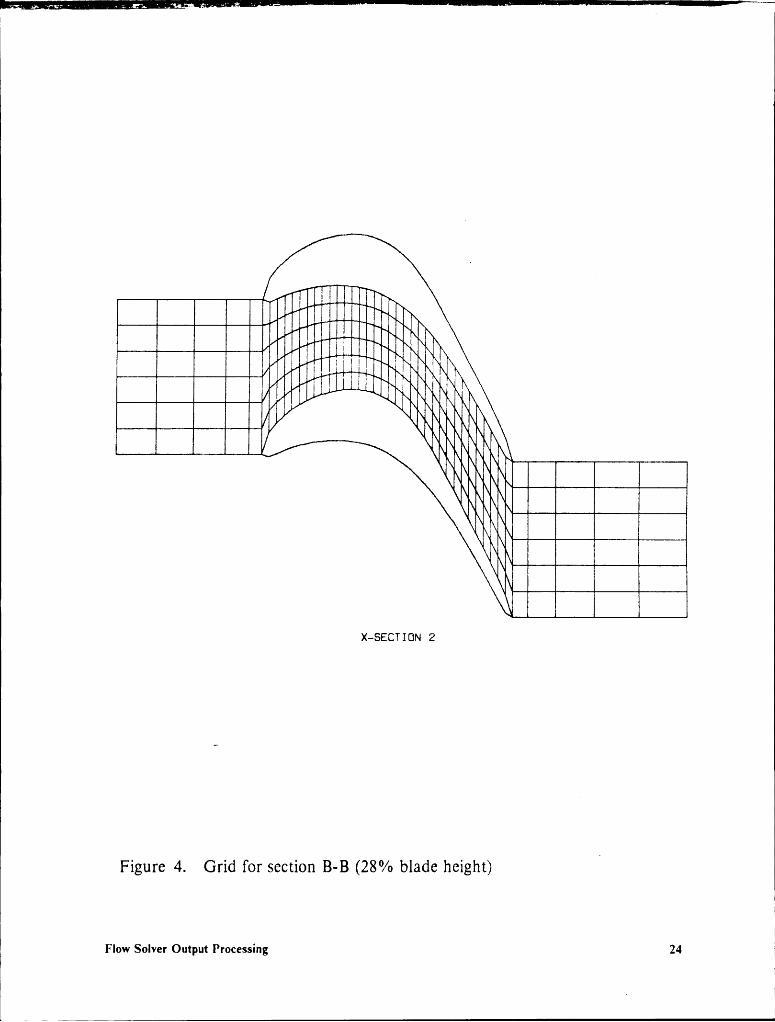
Flow Solver Output Processing

The cascade solver produces aerodynamic data corresponding to a grid which

divides the cascade passage into an array (typically seven axial lines by thirty-tive

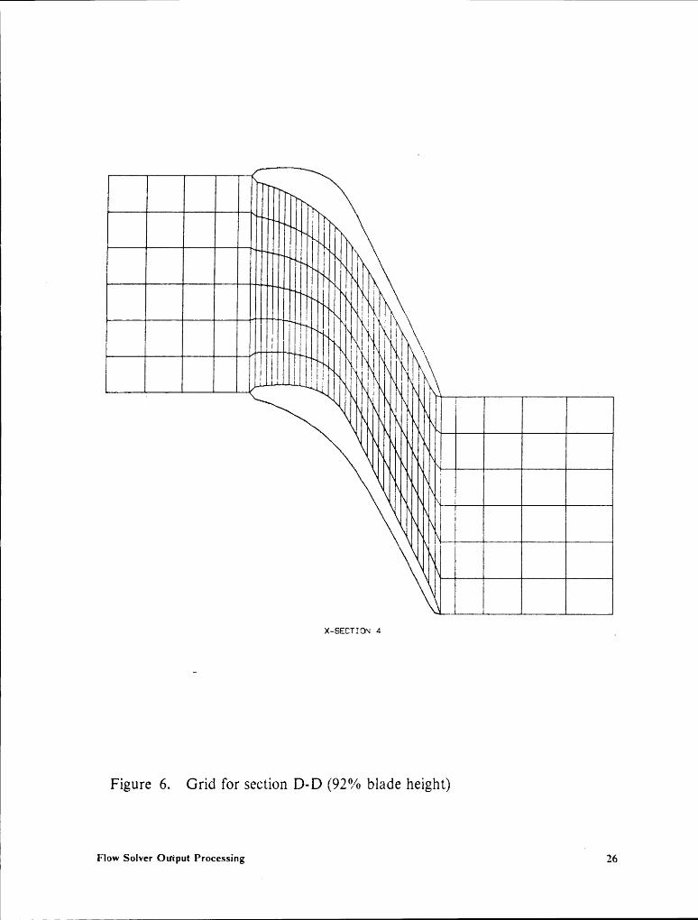
tangential lines). Figures 3 through 6 show the grid for each of the four cross

sections available. Each point corresponds to the center of a polygon in the

computational fluid dynamics code. For each point the associated axial velocity,

. tangential velocity, and relative Mach number are fed into arrays for further

manipulation.

The arrays are used to compute both the axial and tangential components of

the Mach number. By combining these components with the blade geometry,

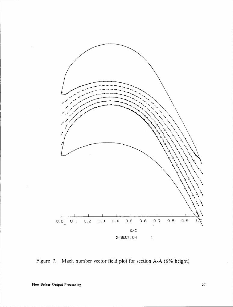
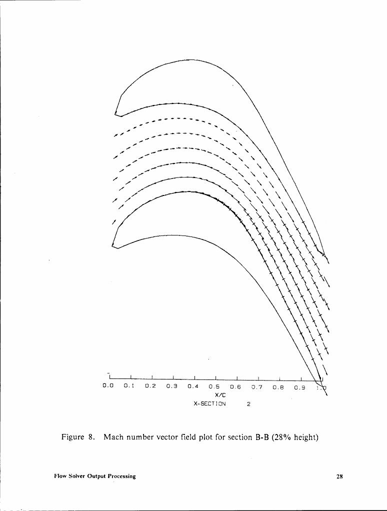
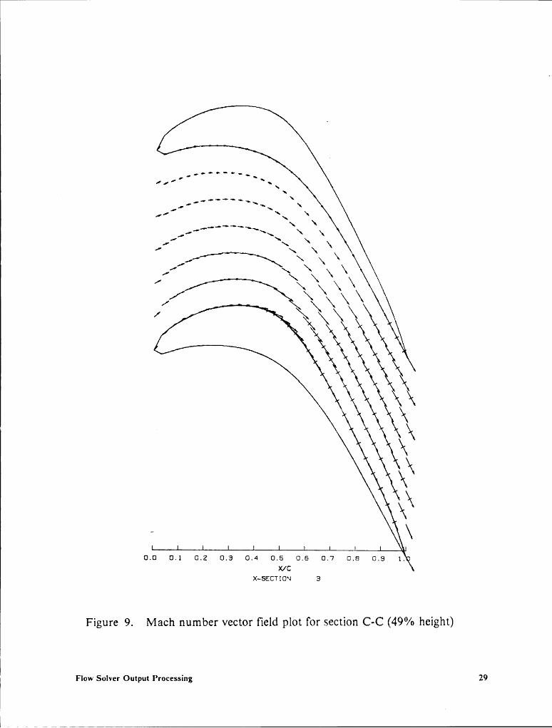
scaled Mach npumber vector field plots are created for the entire grid. The Mach

number field plots for the four blade sections are shown in Figures 7, 8, 9, and

10. The length of each arrow corresponds to the magnitude of the local Mach

number and the arrow orientation indicates the local flow direction. These plotsinclude a cross mark for any vectors corresponding to a Mach number greater1

'

Flow Solver Output Processing 22

--¤u)¢NNQQN

====l’ lllllllllIl;lEEE==N Nu:-——

l|¤———

Figure 3. Grid for section A-A (6% blade height)I

I Flow Solver Output Processing23I. I

in-¤|•¤¤•iIlIlll|l|Il;~¤„--ll"Ili}llllllllIl:g!!}l§~,~lllII§:I§;:««·······=a'䧧E«:~,;;„~—_III’l''-

'° ‘l¤ll!lllg¤¤¤---lu---ll illu---zlllllllllll--

Figure 4. Grid for section B—B (28% blade height)4

uläälälvl(490/° b

II

nuunuuuu„„NI Lili IIIIlI|I|||||IIIu| I I II *‘

I II IIIIII lllllX—SECTIO~ 4 _

Figure 6. Grid for section D·D (92% blade height)

_ IFlow Solver Ouiput Processing Z6I

F II

é

«;i;;1?:;;;?l:§I~.

///’

RW6 x\\xxxäW\X

\\

0.0· 0.l 0.2 0.3 0.4 0.5 0.8 0.7 0.8 0.8 1.

X/CP

X—5ECTl0N 1

Figure 7. Mach number vector field plot for section A-A (6% height) „

Flow Solver Output Processing 27

l______ _.

ZIIII· , , , _ _ g I

1 II • — ‘ ‘-1

x \\x \/ /1

„« \\\\\\\/ // \ \ \\/\/

\) ¤x\\X)?- \

0.0 0.1 0.2 0.0 0.4 0.0 0.0 0.7 0.0 0.0 1.x-sEcT10u 2 F

Figure 8. Mach number vector field plot for section B—B (28% height) iI

Flow Solver Output Processing 28 :

11

-„-——4„ \= ‘

/' \ \ \ \/ \ \ \\ \ \’/ Ö “\

0.0 0.1 0.z 0.6 0.4 0.6 0.6 0.7 0.6 0.6 1.x/cx-66cr10N 6

Figure 9. Mach number vector field plot for section C·C (49% height)

i lFlow Solver Output Processing 29

III

7

6 '·--.

5 •"—•,_‘ 4"¤_

\ \ \,—~—..„ ‘~\ x \3 x \x\ \\ \.. \2 x \ \

‘0.0 0.1 0.2 0.3 0.4 i.5 0.8 0.7 0.8 0.8 1.X-5ECTl(l;fl 4

Figure 10. Mach number vector held plot for section D-D (92% height)

Flow Solver Output Processing 30

than one. The corresponding printed data from the solver shows the supersonicMach numbers are higher as the blade tip is approached.

The Mach number vector plots are convenient for visualizing the output of

the code. Whether the flow is qualitatively correct can be readily determined by

looking at the plots. The plots also help confirm the validity of usingisentropicexit

conditions and sharp trailing edges. Though in reality separation occurs on

blunt trailing edges, the inviscid code adheres to the contour. Therefore, as stated

above, the cusped model of the trailing edges produces both better Mach number

results and better convergence for an inviscid cascade solver. The plots also show

the relative acceleration through the rotor and give a qualitative indication of

shock regions.

A second set of plots produced for code development and future use are

graphs of Mach number vs. gridline. The plots of Mach numbers along the

streamlines through the channel are helpful in locating shock regions and are later

used in the blade temperature programs. Mach number plots for the twenty to

fifty potential lines crossing the streamlines both verify the uniform inlet and exit

conditions and offer further insight into shock formation. Collectively, these plots

also help make clear which effects result from geometry problems and which re-

sult from the aerodynamic boundary conditions.

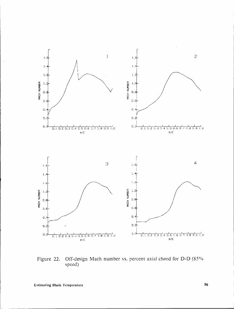
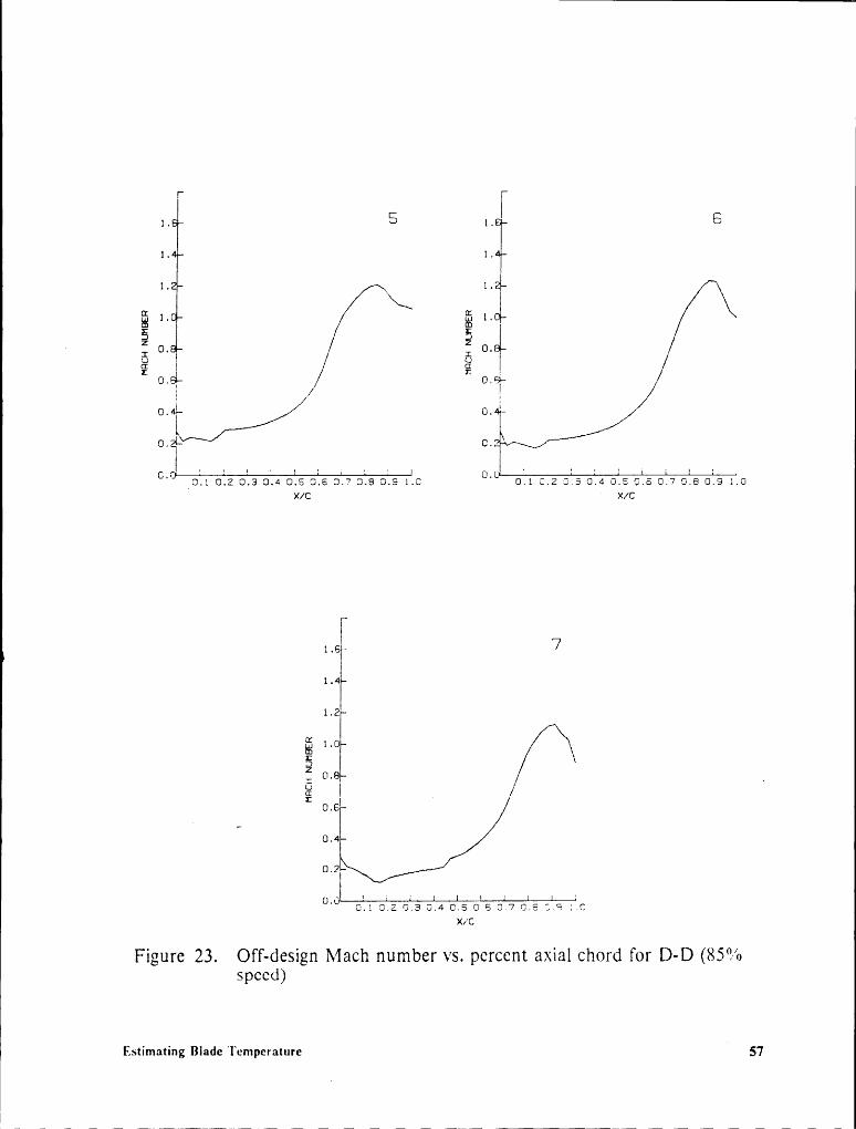
Graphs of Mach number vs. percent axial chord along a streamline reveal

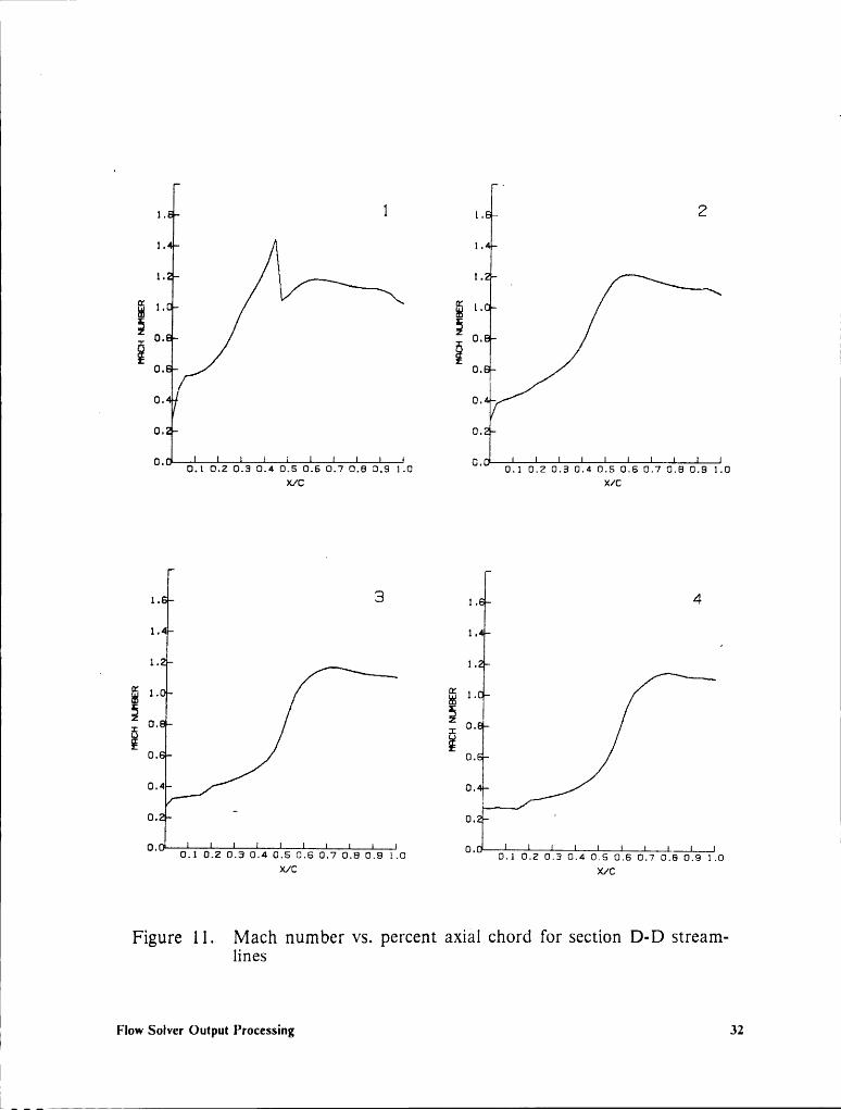
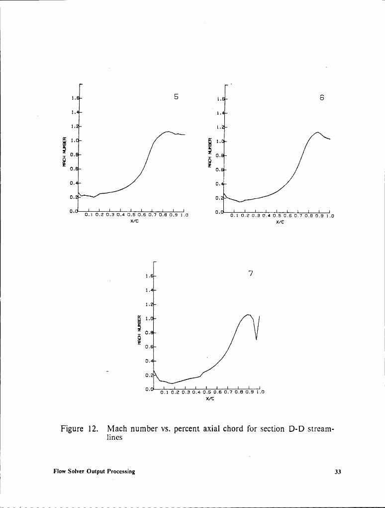
some interesting points that become useful in the final temperature estimating

scheme. The streamline plots for section D-D (92% height) are shown, as repre-

[ sentative examples, in Figures ll and 12. The numbers in the upper right hand

;Flow Solver Output Processing 3l

111

1. 1 1. 2

1. 1.

1. 1. —

§1. ä 1.0. ä 0.0. I 0.

10. 0.

O. O.

O1 0.10.2 0.3 0.4 016 0.6 0.7 0.8 0.91.0 O' 0.10.2 0.3 0.4 0.5 0.8 0.7 0.8 0.91.0 .X/C X/C

1. 3 1, 4

1-4 1.1- 1.

g 1. ä 1,0- 0.0. Q,

Ü·‘i 0.

O. - 0, ‘

O- 0.10.2 0.3 0.4 0.5 0.6 0.7 0.8 0.91.0 O' 0.10.2 0.3 0.4 0.5 0.6 0.7 0.%.0X/C x/rg

Figure ll. Mach number vs. percent axial chord for section D-D stream-lines

1

} 11

ßFlow Solver Output Processing 32 1

111 1

1 1

1 _ _ _

II

1. 5 [_ 6

_ 1-I

1.

1. [_ _

§ 1- ä 1.0- 0.

ä 0- 0.

0- 0.

0- 0.

O' 0.10.2 0.3 0.4 0.6 0.6 0.7 0.6 0.91.0 O' 0.10.2 0.3 0.4 0.6 0.6 0.7 0.6 0.91.0x/c x/c

q 1.6 7

1.4

1.

ä 1.§

0.

0.6

0. l

- 0.2

O' 0.10.2 0.3 0.4 0.6 0.6 0.7 0.6 0.91.0x/0

Figure 12. Mach number vs. percent axial chord for section D·D stream-lines

i Flow Solver Output Processing 33tI .

I II._...............r.r._r_..______

II1

corner of each graph count the streamlines across the cascade from the suction

surface to the pressure surface. The suction surface streamline corresponds to l,

the midstream line to 4, and the pressure surface to 7. (see Figure 10)

The streamline along the suction surface, the one of primary interest, is the

least stable streamline. The imperfect blade smoothness is evident. A shock is

predicted at 42% axial chord. The shock is localized to the region near the sur-

face and may be emphasized because of geometric effects. It certainly weakens

as mid-passage is approached and may be strictly local; in any case it is not very

strong. At these low Mach numbers an isentropic shock model is valid. How-

ever, shocks of this nature are present in every cross section studied. The shock

is weaker and occurs slightly further downstream as the hub is approached, in-

dicating a part-passage three dimensional shock. Shocks are smeared and weak-

ened as the number of axial divisions used in the cascade solver is decreased.

The sharp drop in Mach number at the trailing edge of the suction surface

streamline is caused by the inviscid code following the trailing edge cusp. The

pressure surface streamline plot (number 7) of Figure 12 shows a sharp drop in

Mach number just before the trailing edge. The Mach number vector plot for this

cross section, Figure 10, provides the explanation with reference to the vector

near the trailing edge of the pressure surface. The inviscid flow follows the trail-

ing edge contour, producing an unrealistically low velocity data point. The trail-

ing edge cusp for section D-D is not as sharp as for the other sections, so this

section represents a worst case. This problem clearly illustrates how pressure side1

Flow Solver Output Processing 34 1I

II

effects are numerically communicated to the suction side in computational mod-P

eling. 1

When defining the free stream boundary conditions for the temperature re-

covery routine, some of the mid-passage streamlines will be used to smooth the

surface line values. The smoothing helps to eliminate unwanted effects of the

inviscid assumption and lessens the effects of the rough blade surface contours.

This technique is outlined in the following section.

Flow Solver Output Processing . 35ä11

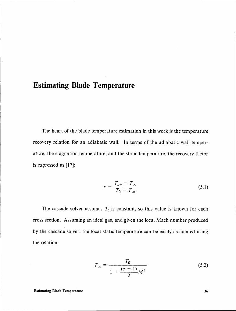
Estimating Blade Temperature

The heart of the blade temperature estimation in this work is the temperature

recovery relation for an adiabatic wall. In terms of the adiabatic wall temper-

ature, the stagnation temperature, and the static temperature, the recovery factor

is expressed as [17]:

T — T,· = .&....;°E’. (5_l)To — Too

The cascade solver assumes TO is constant, so this value is known for each

cross section. Assuming an ideal gas, and given the local Mach number produced

by the cascade solver, the local static temperature can be easily calculated using

the relation:

To12

Estimating Blade Temperature 36 ]111

1. lt is assumed that y = 1.33 for the temperature range encountered in the

n

turbine. This assumption is confirmed by a look into the air tables, as y varies

from only 1.326 to 1.336 in this application [18]. A variable ratio of specific heats

can be added to the code if greater temperature ranges are met.

The major problem with the adiabatic wall relation is knowing the proper

value for r. Values range from 0.83 to 0.91 for flat plates, with the higher values4

applying to turbulent flow [17]. The recovery factor work of Kopelov and Gurov

includes a study of experimental variation of r with Reynolds number on turbine

blades. They found that the recovery factor went up with Reynolds number and

leveled off at a Reynolds number of 2x105 at values bounded by 0.78 and 0.95,

with a mean of 0.87 [19]. The nominal chord-based Reynolds number for the

blade is 5xl0$. Thus turbulent flow is assumed, especially since the leading edge

is not a problem here. Assuming a constant r=0.89 is reasonable, recalling the

favorable pressure gradient in the stage. Consigney and Richards also used

r=0.89 in their turbine rotor heat transfer work with good results [20]. Fortu-

nately, the equation is forgiving with respect to the r value, as a 10% error in r

leads to about a 1% error in the value of Tw in this range, as:

_ Taw = r(T0 — Tw) + Too (5.3)

Another judgement comes into play concerning the choice of local Mach

number to use in calculating local temperature, T,,,. The trouble stems from both

the absence of boundary layer effects and from the local problems that arise dueto digitized geometry. The most critical adjustment is to correct for the less

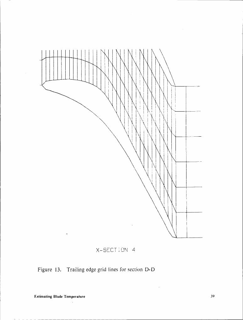
~1Estimating Blade Temperature 37

sharply cusped trailing edge of section D—D. Figure 13 shows how the slopes

ofthestreamlines near the pressure surface change abruptly as they leave the cas-

cade. Note the two streamlines closest to the pressure side trailing edge break

upward substantially in a single axial step, following the trailing edge cusp. The

solver turns the flow to follow the geometry faithfully, causing the unrealistic flow

pattern mentioned previously. The grid outside the cascade has no geometric

boundary conditions to induce turning, so no error is induced in this region. The

imposed condition of periodicity that is necessary in an infinite cascade solver

causes the suction side trailing edge to feel the effects of the pressure side trailing

edge. In this region, geometric problems are compounded. The suction side

trailing edge streamline has a distinct Mach number decrease as shown in plot 1

of Figure ll, even though the suction side surface is relatively smooth. The error

introduced by using mid-passage streamlines as part of the free stream boundary

in the trailing edge area is less than the geometrically-induced inviscid error in-. herent in the surface streamlines.

The method chosen to include the mid-passage streamlines uses the first four

streamlines in percentages that vary from suction to mid-passage and according

to percent axial chord (X/C). Smooth polynomials are used that include gradu-

ally more mid·stream information as the trailing edge is approached. This

smoothing is done in a FORTRAN program loop of the temperature estimating

program. The corrected Mach number plot for section D-D , for example, was

calculated using information from the first four streamlines in fractions thatvaried as follows:

VEsiamatsng Blade Temperature 38

I

I I I I1 I

·

1

~

1 I1 x 1

I\1I1111I1Q;III1"IIII] I

· 1 I I I IYI11.1111II·II1I1

·

II Ill 1

><—SECTlÜ!\l 41

Figure 13. Trailing edge grid lines for section D·D

i

Estimating Blade Temperature 39

PART4 = 0.3 ><(X/C)$PART3

= 0.25 >< (X/C)‘

PART2 = 0.25 >< (X/C)‘

PARTI = 1.0 — (PART4 + PART3 + PART2)0

PARTI, 2, 3,4 correspond to the fraction of the respective streamlines used to

define the free-stream Mach number for the corrected Mach number profile. The

relevant Mach number streamlines range from 1 for the suction surface to 4 for

the mid-passage streamline. This method corrects primarily the trailing edge data

and allows the suction surface streamline to more nearly match the conditions

which a viscous solution would provide. The simple fourth and fifth powerpolynomials cause negligible correction to be made before 50% axial chord. At

this point over 95% of the surface streamline information is retained

(PARTI > 0.95) . At 75% X/C, about 7% each of the second to fourth stream-

lines are used, still retaining greater than 75% of the surface streamline informa-

tion. This drops quickly to about 20% surface information at the trailing edge.

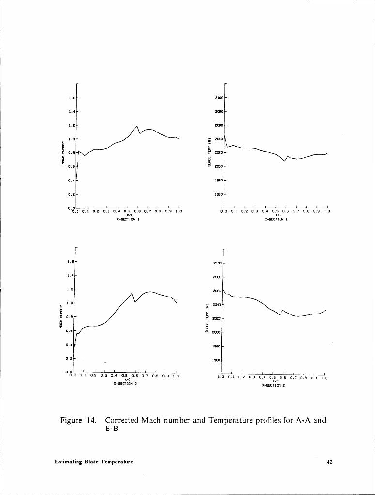
The corrected Mach number profiles for all four cross sections are shown in Fig-

ures 14 and 15. Especially note the corrected Mach number plot for section D-D

(section 4), as compared to the four uncorrected streamline plots for section D-D

of Figure 11; ihe Mach number drop at the trailing edge is restricted while re-

taining the nature of the original curve. As a guideline in choosing the constant

factors for the streamline fractions, an attempt was made to match the trailing

edge Mach number to the given surface line value. Sections A-A, B-B, and C-C

were smoothed in the same manner, however the polynomial constants varied to

Estimating Blade Temperature 40 I

include less midstream data as section D-D was the worst case. Actually, theU

smoothing method employed for developing the corrected Mach number curves

of Figures 14 and 15 has little effect on the original curves, except near the trail-

ing edge of the blades, where the unrealistic acceleration is reduced.

Once a satisfactorily smooth Mw curve is created, a Tw, curve is computed for

each of the four cross sections using the adiabatic wall recovery factor equation

(5.3). As each cross section may have a different number of axial points, any of

the axially less—populated curves are expanded to iifty axial points to create four

fifty-point temperature lines. The right hand plots of Figures 14 and 15 consist

of the temperature lines for each of the cross sections. The four lines form a four

by fifty temperature grid on the blade surface. This array is used as a data base

from which the trace path calls values. Each point in the array corresponds to a

unique value of percent axial chord and one of the four possible percent blade

heights in non-dimensional coordinates.

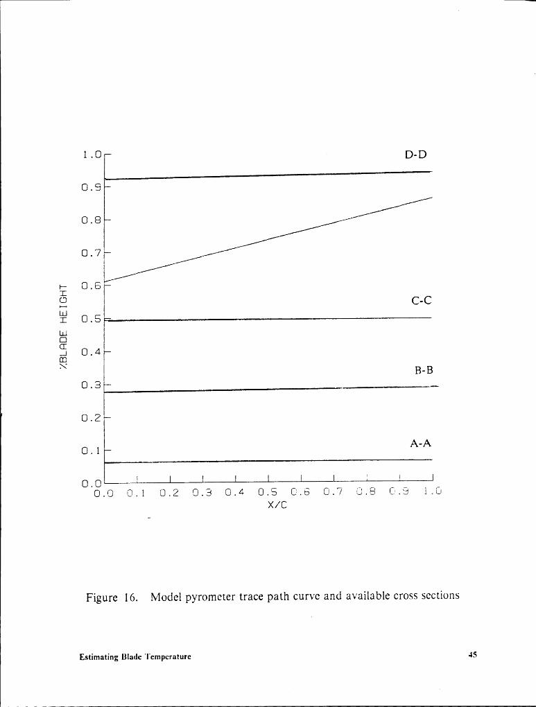
Ideally, the exact path the pyrometer reception ’spot’ sweeps out along a

blade in non-dimensional coordinates as the blade passes would be known in the

non-dimensional coordinates. This is a rather complicated geometric problem

being solved in a parallel effort using the Virginia Tech Mechanical Engineering

Computer Aided Design Facility. Preliminary results from the CAD work of

Williams [21] shows the path can be modeled by the curve

Y = .25 >< (X/C) + .611 (with Y being the percent blade height) shown, along

with the positions of the four cross sections of available temperature information,

in Figure 16. To generate the model signal, fifty points from the model

Estimating Blade Temperature 4l1

l

1.8 2100

1.4 2®0

1.2 ZGO

1.0 E 2040A

§ s0.8 r—· 2020

E ä0.6 m 2000

0.4 LEO

0.2 1560

0.1 0.2 0.3 0.4 0.5 0.6 0.7 0.8 0.9 1.0 0.0 0.1 0.2 0.3 0.4 0.5 0.6 0.7 0.8 0.5 1.0' X/C X/CX··SECT10N 1 X-6ECT10N 1

*6 21CD*‘ zoao*2 zoao1.0 wm

g0.8 2020

i0.4 lg) '0.2 _ lg

08.0 0.1 0.2 0.3 0.4 0€C0.6 0.7 0.8 0.3 1.0 0.0 0.1 0.2 0.3 0.4 0; 0.6 0.7 0.8 0.9 1.0CX-SECTXON 2 X—EET1¤‘~2 2

Figure 14. Corrected Mach number and Temperature profiles for A-A andB·B

Estimating Blade Temperaturel

42

II

1.6 ZICD

1.4 ZH)

1.2 ZH)·

1.0 E Z340

§ a0.8 v- Z20

E 50.6 Ü ZGIJ

0.4 XK

0.2 1£3{

0Ig.00.1 0.2 0.3 0.4 0.5 0.6 0.7 0.8 0.3 1.0 0.0 0.1 02 0.3 0.4 0.5 06 07 0.8 0.3 1.0X/C X/C

X—§CT1IN 3 X—§IIIT1CN 3

1.6 zum

1.4 zum1.2 2060 *

I a ‘·°E 2040

g °·° gl 20205 50.6 ad 2000

°·‘ isaoI 0.2

· [S60

°Ig.0 0.1 0.2 0.3 0.4 0*äc0.I6 0.7 0.8 0.9 l.0 0.0 0.1 0.2 0.3 0.4 0.5 0.5 0.7 0.8 0.3 1.0X-SECTIUN 4 4

Figure 15. Corrected Mach number and Temperature proüles for C-C andD·D

Estimating Blade Temperature 43

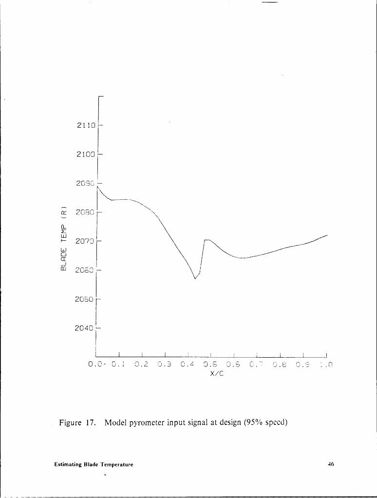
Ipyrometerintersection curve are used to linearly interpolate temperature values

from the two nearest cross sections using axially corresponding points of the ar-

ray. A model pyrometer input signal for design conditions (95% speed) is re-

· presented in Figure 17. This result is a culmination of all the previous curves and

should prove to be a valuable tool in evaluating pyrometer performance.·

The pyrometer input signal model of Figure 17 represents a solution for de-

sign point conditions on a test stand. Off-design solutions could be easily

produced if the aerodynamic data for the off-design speeds were available. With

the lower Mach numbers of the off-speed case, the flow field is simpler for the

cascade solver. Convergence time is reduced and shock effects lessen or disap-

pear.

With no off-design conditions given for this stage, they are estimated incor-

porating severalassumptions. To accurately model off-design conditions a com-

plex cycle analysis would have to be done which would require performance maps

for the various engine components. Unfortunately this information is probably

more difficult to obtain from the manufacturer than off-design stage

aerothermodynamic boundary conditions. A less complex method for estimating

off-design conditions based on data obtained from engine tests is developed be-

low. The off-design case presented is for an 85% speed case, as compared to the

95% speed (design) case presented previously, that used data given by the engine

manufacturer. For free-vortex blading the temperature change across a turbine I

stage can be expressed by [1 1]: _ I

Estamaung Blade Tcmpmwm 44 I

I1

1 .0 - Q-Q0 .3

0 .0

0 . 7

1—- 0.0IE c-CEI? 0.6L1.IE.1 0.4

B-B0.3 ---....

0 .2

0. 1 A’A

0 .00.0 0.1 0.2 0.3 0.4 0.0 0.0 0.7 0.3 0.3 1.0X/C

Figure l6. Model pyrometer trace path curve and available cross sectionsI

111

Estimating Blade Tempcraturc 45 II

I

2110% U2100I2050 Q

Q wwixxCC ILu

MJI5D

CI.J@1 2050I

2050[2040

I l I 1 1

0.0- 0.1 0..2 0.3 0.41 0.5 0.5 0.7 0.13 0.*3 1.0X/C

. Figure 17. Model pyrometer input signal at design (95% speed)1

Estimating Blade Tcmperature 46 I

I

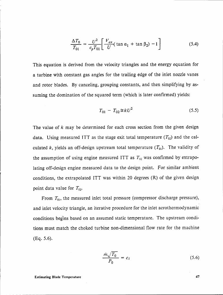
tan al + tan B2) -1] (5.4)

This equation is derived from the velocity triangles and the energy equation for

a turbine with constant gas angles for the trailing edge of the inlet nozzle vanes' and rotor blades. By canceling, grouping constants, and then simplifying by as-

B

suming the domination of the squared term (which is later contirmed) yields:

BTUI — T02;kU2 (5.5)

The value of k may be determined for each cross section from the given design

data. Using measured ITT as the stage exit total temperature (T02) and the cal-

culated k, yields an off-design upstream total temperature (To,). The validity of

the assumption of using engine measured ITT as T02 was coniirmed by extrapo-

lating off-design engine measured data to the design point. For similar ambient

conditions, the extrapolated ITT was within 20 degrees (R) of the given design

point data value for T02.

From TO., the measured inlet total pressure (compressor discharge pressure),

and inlet velocity triangle, an iterative procedure for the inlet aerothermodynamic

conditions begins based on an assumed static temperature. The upstream condi-

tions must match the choked turbine non-dimensional flow rate for the machine

(Eq. 5.6).

I= C1 (5.6)

Estimating Blade Temperaturel

47

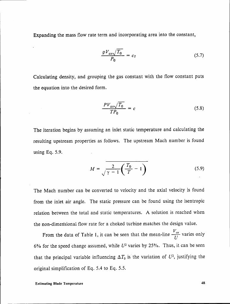
Expanding the mass flow rate term and incorporating area into the constant,I

_PO cz (5.7)

Calculating density, and grouping the gas constant with the flow constant puts

the equation into the desired form.

PV...,gTJ‘ = 5.8TP0 C ( )

The iteration begins by assuming an inlet static temperature and calculating the

resulting upstream properties as follows. The upstream Mach number is found

using Eq. 5.9. .

2 ToM = ——— —— — 1 5.9V T - T ( T ) ‘ )

The Mach number can be converted to Velocity and the axial Velocity is found

from the inlet air angle. The static pressure can be found using the isentropic

relation between the total and static temperatures. A solution is reached when

the non-dimerisional flow rate for a choked turbine matches the design Value.V

From the data of Table l, it can be seen that the mean-line—Ü’i

varies only

6% for the speed change assumed, while U2 varies by 25%. Thus, it can be seen

that the principal Variable influencing AT., is the Variation of U2, justifying the

original simpliiication of Eq. 5.4 to Eq. 5.5. l

Estimating Blade Temperature 48l

—

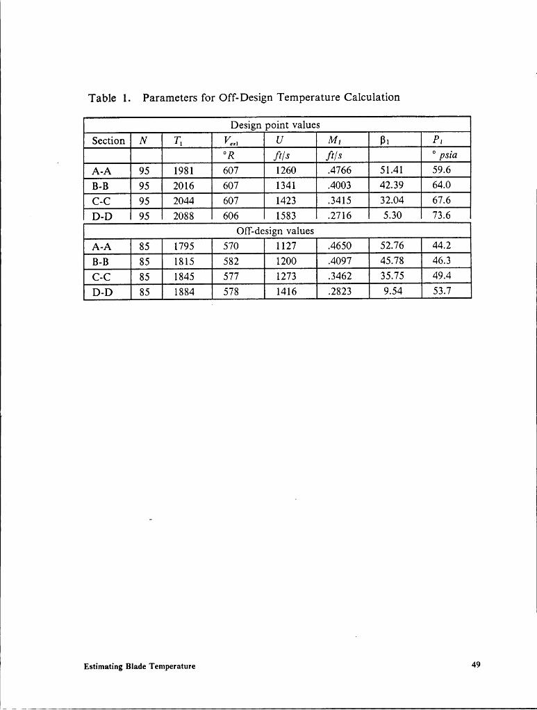
I1

Table l. Parameters for Off-Design Temperature Calculation

Design point valuesSection N 7] V„, U M1 B1 Pß/S

-

° waA-A 95 ß 607 1260 .4766 51.41 59.613-13 95 2016 607 1341 .4003 42.39 ßC-C 95 2044 607 1423 .3415 32.04 67.6D-D 95 2088 606 1583 .2716 5.30 73.6

OIT-design valuesA·A 85 1795 570 1127 .4650 52.76 44.2B-B 85 1815 582 1200 .4097 45.78 46.3cz-c 85 1845 577 1273 .3462 35.75 ß

85 1884 578 ß .2823 9.54 53.7

Estimating Blade Temperature 49

Exit conditions are found from the inlet conditions through a similar iterativeU

procedure that includes the assumptions of constant relative total temperature

and pressure through the rotor. With the relative exit gas angles assumed con-

stant, a solution is found for the guessed exit static temperature when the condi-

tions for conservation of mass are met. The upstream and downstream

conditions then serve as inputs to the flow solver as before.

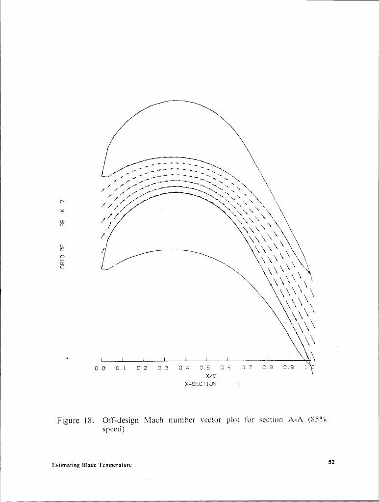
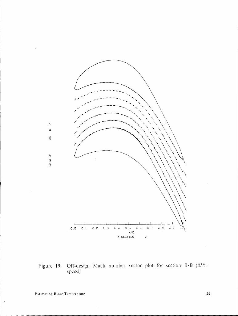
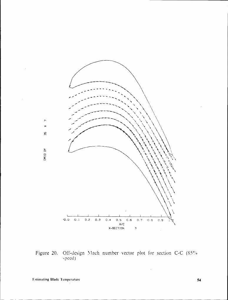
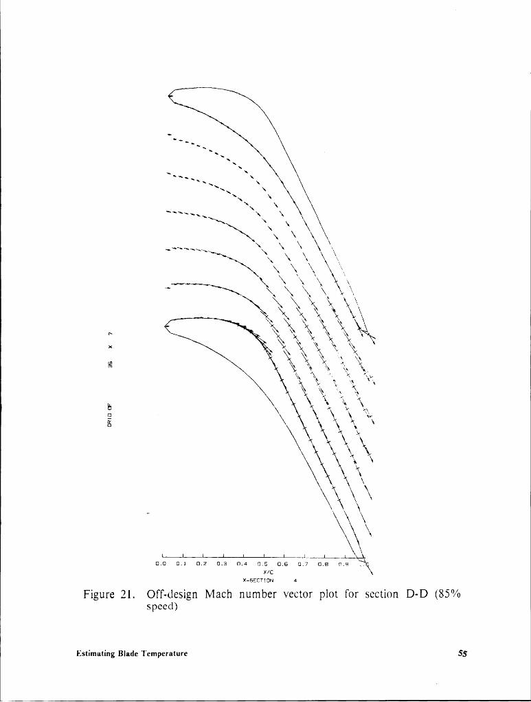
The off-design Mach number vector plots are shown for the four cross

sections in Figures 18 through 21. The inlet angles of attack are higher, and the

supersonic regions have become smaller or disappeared, as in the root section case

(Figure 18). The streamline Mach number traces for section D-D are shown for

the 85% speed case in Figures 22 and 23. As compared to the design point traces

of Figures 11 and 12, the off-design flow has greater near-trailing-edge recom-

pression. Trailing edge smoothing is still necessary, especially for section D-D.

The corrected surface Mach number graphs and corresponding temperature

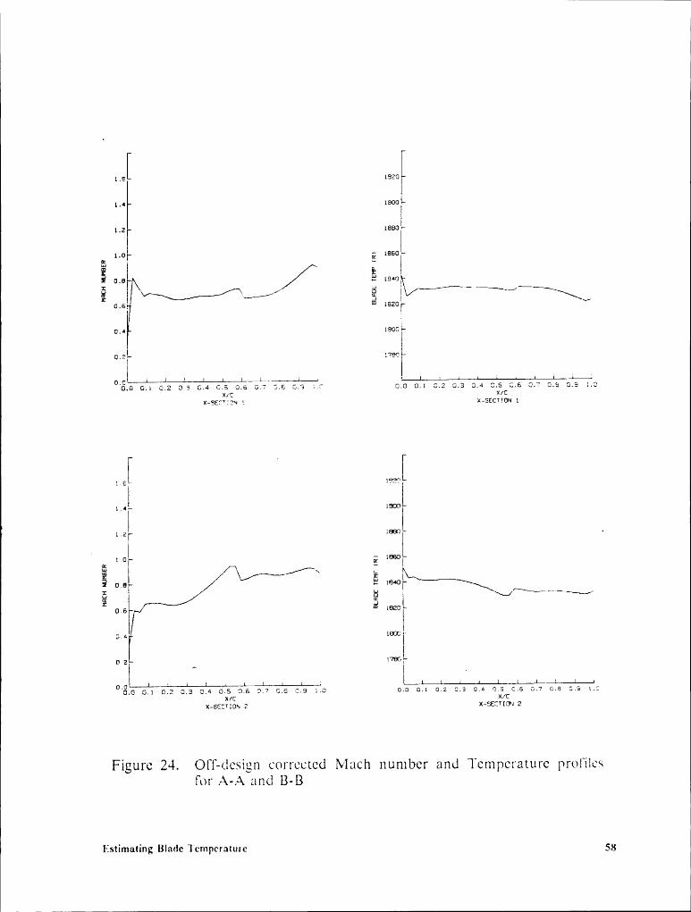
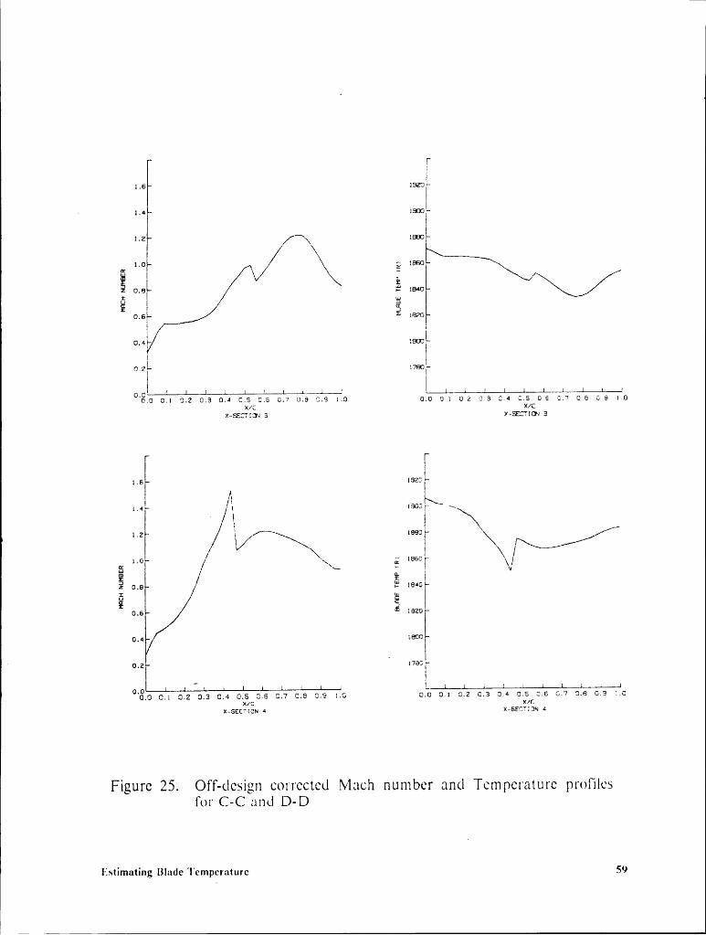
profiles are shown in Figures 24 and 25. Again, the off-design traces show more

trailing edge recompression and lower Mach numbers. The predicted temper-

ature profiles are similar in nature but are nearly 200 degrees (R) lower. The

interpolated model pyrometer signal shown in Figure 26 reflects the recom-

pression region in a flatter temperature trace. The temperature change shown is

dramatic for a 10% wheel speed change. When the trace paths for the design and

off-design case are plotted together to show their relative emissive power, Figure

I27 results. This is a non—dimensional plot of ratio of the emissive power of the

{

Estimating Blade Temperature 50

two cases compared to a blade at a uniform temperature of 1800 degrees (R).

This Figure shows the sensitivity potential of a pyrometer. ·

_ The off-design results will be useful in pyrometer development, and are easily

produced once the aerothermodynamic boundary conditions are known. In the

following section possible improvement areas are targeted.

Estimating Blade Tempemure si

1

j /'\s

· // \\\\(O/ \ \\\

/ \\\/Ä\ ‘ ‘

x \\\ \ ‘N1N‘

N\\\ .\

V 0.0 0.1 0.2 0.3 0.4 0.5 0.5 0.7 0.3 0.3 1.X/C \

X—SECTl0N 1

Figure 18. OIT-design Mach number vector plot for section A-A (g85‘€~’ospeed)

Estimating Blade Temperature 52

III

~· \\

‘\/‘\‘\X

/ “~ \\in/ \¤ \ \ — \~(U\ x I *~ \‘ ~LL\“

\X‘ ‘

O.Ü Ü.1 OZ O.: Ü.4 Ü.;/C Ü.5O.9X-SECTION2

Figure 19. Ol“t“-design Mach number vector plot l‘or section B-B (85%speed)

listimuting B|ade'|'cn1pcraturc 53

I

I

."ll ,·*°°""—\

" \11

X X \

//’ \ \x \ \ \

/ x>< 1 \ \/-/(IQu.

$«¤ a ‘ I0 esLJ *\\x\\

\

· \\

I I 5

x/c \x-s6cvi¤N a _

Figure 20. Off-design Mach number vector plot for section C-C (85%speed)

Iistimating Blade Temperature 54

l

ll

x\ \\\ \

x\\ \\_X.

XX: \‘ \x“““"\ X, \ xX X \\

Xx

Vx\ \ A\ l “

\

\\ li

'0.0 0.1 0.2 0.3 0.4 0.5 0.5 0.7 0.5 0.9 ..

X/CX—5ECTl0N 4

Figure 21. Off-design Mach number vector plot for section D-D (85%speed)

Estimating Blade Temperature 55

I

1. 1 1. 2

1. 1.1CI OCä 1- é 1.01—ä 0. \/ i 0.LJ LJ

0. 0. _I1er0. 0.2l-

0.10.1 0.2 0.3 0.4 0.5 0.6 1].7 0.9 0.9 1.0 Of 0.1 0.2 0.3 0.4 0.6 0.6 0.7 0.6 0.9 1.0

X/C X/C

1 I1.61- 3 IFT 41.4‘» 1-T1,2;

1.5 5Z 09 Z G-I ‘ 5LJ% { ¥

@,5l 0.

0.4+-Ä0.2 - 0-J

0.0 0.10.2 0.3 0.4 0.6 0.6 0.70‘.9

0.91.0 O. 0.10.2 0.3 0.4 0.6 05.6 0.7 0.6 0.91.0X/C X/C

Figure 22. Off-design Mach number vs. percent axial chord for D-D (85%1 speed)

Estimating Blade Temperature 56 I

I

1

I

“ I1. 5 1. 6

1. 1.

1. 1.

§ 1. ä 1. I§ äI 0. I 0.ä ä .0.6L 0.6—I .4 IÜ. I

0.zIL 0.C _0.1 0.2 0.3 0.4 0.6 0.6 0.7 0.6 0.6 1.0 O 0.1 0.2 0.3 0.4 0.6 0.6 0.7 0.6 0.6 1.0

x/0 xzc

1.6 7

1.4

1.2

II 1.0§2/)§

I0.6I_

0.4

0.2*‘_ ‘ _ '0.1C.c 0.3 0.4 0.6 0.6 0.7 0.6 -.911]

X/C

Figure 23. Off-design Mach number vs. percent axial cherd for D-D (85%speed)

Estimating Blade Temperaturc 57

I

1.1s*Q 16201.4|» 160016801.0 1650

EE 0.8’>

/\

E 334:}I .1,1 '

,.-——·——~— .

0.6_ ¤= 1620 10,4% lßüüt0.21 1790,¤_G*__.1_.1i;._.1._.&._;T.1—_1...1_0„”0.00.1 0.2 0.6 0.4 0.6 0.6 0.7 0.6 0.6 0.0 0.1 0.2 0.6 0.4 0.5 0.6 0.. 0.6 0.6 1.0x/0 x/1:x-61-irT*1c~1 1 x-56cT10u 1

3 5* 1*320*

1.4* 1370**1.2 1680 ·

l 1 0 ; 1860ä Q2 (15 1840E*5gEE0.6[f$/ 1620

ÜJUE 18C0i·gg _ 17%*

0.0 *”0.00.1 0.2 0.6 0.4 0.5 0.6 0.7 0.6 0.6 1.0 0.0 0.1 0.2 0.6 0.= 0.6 0.6 0.7 0.6 0.6 1...x/c X/C

X-BECTION z X-EECYICN 2

Figure 24. Off-design correeted Mach number and TCIT1pCI'&1L1I“C proiilcsfor A-A and B-B

Estimating Blade Tcmpcraturc $3

1.6 192C{» 1.4 1330

1.2 1m0

1.0 IECZ ..

Z 0.8 •— 1840

Q äO.6i·· ii 16200.4-

I I I I‘

' ' ' I '

00.0 0.1 0.2 0.3 0.4 0.6 0.6 0.7 0.6 0.6 1.0 0.0 01 0.2 9.3 0.4 0.6 OE 0.7 0.6 0.6 1.0x/0 x/0

x-6..6:71:11 3 x--$.1*101 3

L4- ISZOQ1 Ll.4l— ISÜÜ ’ s1.2% ‘°°°¥'1.0 ~\L gIBBOV2% l»2 0.6 E 1840

5 6g0.6 Ei 1620'

0.4 IEC?0.2

l1735***

- Ql00.00.1 0.2 0.3 0.4 0.6 0.6 0.7 0.6 0.6 1.0 0.0 0.1 0.2 0.3 0.4 0.6 0.6 0.7 0.6 0.6 :.0xzc x/0

x-66011011 4 x-661:r1;1~ 4

Figure 25. Off-design eorreeted Mach number and Temperature profilesFor C—C und D-D

Hstimating Blade Temperaturc 59

I

II

1910%190OI-1890I-

E 1000=\/A[L l /L1.lX I1-1070LI.!ES—I l I\\ „4 /3/G3 1000I—1850*

4mm?

I I I I I I I I I 1

0.0 0.1 0.0 0.41 0.0 0.0 0.7 0.0 0.0 :.0></0

Figure 26. Model pyrometer input signal for off-design (85% speed)

listimating Blade Temperature 60

I@11

.761

.6 }—sr ·:*.1. . e.}

IG IQ , IS; 1 .¢ 1---I\ I. _ I

3. 1 .5 I->•< IIF *2 IN/*";_1 .

I ICMC? @.1 CRX C.} Ü.! CR; Ci.}

X/C

. Figure 27. Relative emissive power comparison berween 85% and 95%speed

III

Iistimuting BladeTemperaturcI

Conclusions E

The results of this thesis give qualitative and quantitative views of a

pyrometer signal not readily available previously. The goal of producing a model

signal was successfully met. At this point the details of the model signal will be

impossible to capture with the pyrometer system. For this application, with a

high blade passing frequency and moderate temperatures, the hope for distinctly

separated blade signatures is weak. Even a pyrometer system with a 1MHz

sampling frequency capability could only capture about five target spot points

per blade. The path the pyrometer sight beam traces (see Figure 16) starts at the_

leading edge at mid-span and sweeps toward the tip region at the trailing edge.

The trend for blade temperatures is to increase as blade height increases and to

decrease as percent axial chord increases. These trends seem to cancel out to

some degree for this trace path so the temperature input signal will tend to be

rather flat. The shock structures may also be difficult to capture by theu

y lconciusaons 62 l‘ l

u

pyrometer because of the unsteadiness of shocks and the temperature smearing

caused by conduction.4

While there is room for improvement in the aerothermodynamic approach,

it already provides a model signal with greater detail than current pyrometers can

capture. With better boundary conditions, both aerodynamic and geometric, thisprocedure should yield a model signal with sufiicient accuracy to evaluate the

6 performance of experimental pyrometer systems.

concnusnms 63 !l

r

l

Future Work Recommendations

The work in this paper represents a preliminary method for estimating tur-

bine blade temperatures from the flow conditions. There are several areas where

improvements can be made in continuation of the project. This work used a

two-dimensional code, but three-d—imensional solvers are becoming prevalent and

offer additional accuracy [4,5]. Much of the set-up work will be simplified when

codes with interactive boundary layer methods are available. Solutions will be

more accurate and geometric effects will be minimized. Advanced codes may

soon be able to handle separation bubbles and the wake flow [22].

lncluding heat transfer effects is another area targeted for study. Certainly

for any cooled blade stages, the code must take the cooling flows into account.

Even the uncooled blades of this study have a certain degree of conduction to the

turbine disk and from the suction to pressure side, that if included in the analysis,

would improve the results further. Axial conduction and the unsteadiness of

shock attachment may also smooth the temperature pro_files to some degree. Se-

Future Work Recommendations 64

4veral conduction models are presented by Maccallum which model the thermal

response of blading to engine acceleration if modeling transients is desired [23].

The work of Brown and Martin suggests that the effects of secondary flows may

increase heat-transfer coefficients, and should be included in rigorous analytical

projects [24].

A detailed cycle analysis would improve the off-design aerothermodynamic

boundaiy conditions. However, additional data from the manufacturer may

beeasierto obtain. The effects of ambient conditions on the turbine temperature

may also be handled in a more sophisticated manner than a non-dimensional flow

parameter. Variable specific heats may be added to the program to further im-

prove accuracy, or to handle several different stages. In a case where substantial

laminar regions exist, a relationship between the recovery factor and Reynolds

number should improve the accuracy of the results, although at low Mach num-

ber recovery factor errors are inherently minimized as the difference in total

temperature and adiabatic wall temperature is small.

An area that needs future attention is improvement in matching the actual

engine operating point to the aerothermodynamic procedure to compare the ex-

perimental to _the analytical data. High pressure turbine wheel speed, ambient

conditions, ITT, and compressor discharge pressure are available and should be

adequate for initial comparisons. Including fuel flow rate may be a useful addi-

tion to the input as an indicator for total temperatures.

Future Work Reeommendetions 65

I

The number of the suggested improvements to the procedure that are incor-

porated into a program will depend on the accuracy desired and availability of

inputs and cascade solvers.

t Future Work Recommendations 66

‘ I

II

References I

1. Cook, D.L., "Development of the JTl5D-l Turbofan Engine," SAE Pa-per 720352, pp.1-10

2. Zachirov, Zhuikov, Panteleev, and Trushin "1nfluence of Heat Leakageon Accuracy of Unsteady Heat Transfer Coefiicient Determination inTurbine Flow Passage," Izvestia VUZ. Aviatasionnaya Teknika 1975, v.18, No. 3, pp.14l-146

3. Hassel, J., Personal Correspondence, Litton Poly-Scientific Blacksburg,VA, 20 March 1987

4. Van Hove, W., "Calculation of Three-Dimensional, Inviscid, RotationalFlow in Axial Turbine Blade Rows," Journal of Engineering for GasTurbines and Power April 1984, v.lO6, pp.430-436

5. Holmes, D.G.,Tong, S.S, "A Three-Dimensional Euler Solver forTurbomachinery Blade Rows," Journal of Engineering for Gas Turbinesand Power April 1985, v.l07, pp.258-264

6. Barber, R., "A Radiation Pyrometer Designed for In-Flight Measure-ment of Turbine Blade Temperatures," SAE Paper 690432, pp.1-10

7. Atkinson, W.H., and Strange, R.R., "Pyrometer Temperature Measure-ments in the Presence of Reflected Radiation," ASME Paper 76-HT-74,pp.1-8

I8. Douglas, J., "I-Iigh Speed Turbine Blade Pyrometry in Extreme Environ- I

ments," "Measurement Methods in Rotating Components of III

t References 67 I. III

1

Turbomachinery," ASME Ji. Fluids Eng. and Gas Turbine ConferenceNew Orleans, LA March 10-13, 1980 pp.335-343

9. Benyon, T.G.R., "Turbine Pyrometry- An Equipment Manufacturer’sVieW," ASME Paper 81-GT-136, pp.1-5

10. Camus, J.J., Denton, J.D, Scoulis, J.V., and Scrivener C.T.J., "An Ex-perimental and Computational Study of Transonic Three-DimensionalFlow in a Turbine Cascade," Journal ofEngineering for Gas Turbines andPower April 1984, v.106, pp.4l4-420

» 11. Hill, P.G., and Peterson, C.R., Mechanics and Thermodynarnics of Pro-pulsion, Addison—Wesley Publishing Co.,Inc., Reading, MA 1965, p.305

i 12.. Jane’s All the World’s Aircraft 1986-87 Jane’s Publishing CompanyLimited, London 1986, pp.877-878

13. Private Correspondence, Pratt and Whitney Canada Inc., 30 May 1986

14. Micklow, Gerry J., Personal Communication, Virginia Tech, Blacksburg,VA, November 1986

15. Caspar, J.R., Hobbs, D.E., and Davis, R.L., "Calcu1ation of Two-Dimensional Potential Cascade Flow Using Finite Area Methods," AIAAJournal January 1980, v.l8, No. 1, pp.l03-109

16. Essers, J.A., and Kafyete F., "Application of a Fast Pseudo-Unsteady. Method to Steady Transonic Flows in Turbine Cascades," Journal of

Engineering for Power April 1982, v. 104, pp.420-428

17. Saad, M., Conipressible Fluid Flow, Prentice Hall, Inc., lnglewood Cliffs,NJ 1985, pp.22-23

18. Reynolds, W.C., Thermodynamic Properties in S1, Dept. of MechanicalEngineering, Stanford University, Stanford, CA 1979, pp.6,7

19. Kopelev, S.Z., and Gurov, S.V., "Concerning the Determination of theEquilibrium Temperature of Blades for Streamline Flow Past Them atHigh Velocity," Izvestgza Akademii Nauk SSSR. Energetica i Transport1976, v.l4, No. 4, pp.l27-132

20. Consigney, H., and Richards B.E., "Short Duration Measurements ofHeat Transfer Rates to a Gas Turbine Rotor Blade," Journal of Engi-neeringfor Power ASME Paper 81-GT-146, pp.1-9

References 68

21. Williams, David A., Personal Communication, Virginia Tech,Blacksburg, VA, 13 April 1987

22. Sieverding, Stanislas, and Snoek, "The Base Pressure Problem inTransonic Turbine Cascades," ASME Paper 79-GT-120, pp.1-12

„ 23. Maccallum, N.R.L., "Mode1s for the Representation of TurbomachineBlades During Temperature Transients," ASME Paper 76-GT—23, pp.l-8

24. Brown, A., and Martin B.W., "A Review of the Bases of Predicting HeatTransfer to Gas Turbine Rotor Blades,” ASME Paper 74-GT-27, pp.1-12

I~ I

IReferences _ 69

V

I_ _.