Maximum Likelihood Estimators For Spatial Dynamic Panel ... · Spatial econometrics deal with the...

Maximum Likelihood Estimators For Spatial Dynamic Panel Data

With Fixed Effects: The Stable Case

Jihai Yu∗

February 25, 2006

Abstract

This paper tries to explore the asymptotic properties of maximum likelihood estimators for spatial

dynamic panel data with fixed effects when both the number of time periods T and number of individuals

n are large. When n is proportional to T or T is relatively large, the estimator is√

nT consistent and

asymptotically normal; when n is relatively large, the estimator is consistent with the rate T and has

a degenerate distribution. The possible contribution of the paper is that it establishes the property of

MLE of spatial dynamic panel when both T and n are large.

JEL classification: C13; C23

Keywords: Dynamic panels; Maximum likelihood estimators; Spatial econometrics∗I am grateful to Prof. Lung-fei Lee and Prof. Robert de Jong for their invaluable guidence and comments.

1

1 Introduction

Spatial econometrics deal with the spatial interaction of economic units in cross-sectional and/or panel

data, and have received much more attention recently. The spatial autoregressive (SAR) model by Cliff

and Ord (1973) has received the most attention. It extends the autocorrelation in time series to spatial

dimensions. Early development in estimation and testing is summarized in Paelinck and Klaassen (1979),

Doreian (1980), Anselin (1988,1992), Haining (1990), Kelejian and Robinson (1993), Cressie (1993), Anselin

and Florax (1995), Anselin and Rey (1997), and Anselin and Bera (1998).

For the dynamic panel version of the SAR, to the best knowledge of the author, there is no work done so

far on the topic where the number of time periods T goes to infinity. When T goes to infinity, not only we

have interaction between cross-sectional units, the dependence between time series will also play an important

role. This paper tries to explore the properties of maximum likelihood estimators for spatial dynamic panel

data model with fixed effects when both the number of time periods T and number of individuals n are large.

The paper is organized as follows. In Section 2, stability is defined and a sufficient condition for stability

of spatial dynamic panel is given. We will study the stable model and the properties of the estimators will

be derived. For the case the model is not stable, properties of the estimators will be derived in a separate

paper. Section 3 establishes the consistency and asymptotic distribution of concentrated MLE estimators

when the spatial dynamic panel is stable. The proof follows closely from Lee (2001b) and the relevant LLN

and CLT are replaced with the array counterparts. It turns out that when n is proportional to T or T is

relatively large, the estimator is√

nT consistent and asymptotically normal; when n is relatively large, the

estimator is consistent with the rate T and has a degenerate distribution. Section 4 concludes the paper.

Some useful lemmas and proofs are collected in Appendix.

2 Conditions for Stability

The model is

Ynt = λ0WnYnt + γ0Yn,t−1 + cn + Vnt t = 1, 2, ..., T (2.1)

where Ynt = (y1t, y2t, ..., ynt)′ , Vnt = (v1t, v2t, ..., vnt)′ and vit’s are i.i.d. across t and i, Wn is n× n weight

matrix, which is predetermined and defines the dependence between cross sectional units yit, and cn is n× 1

vector of fixed effects.

2

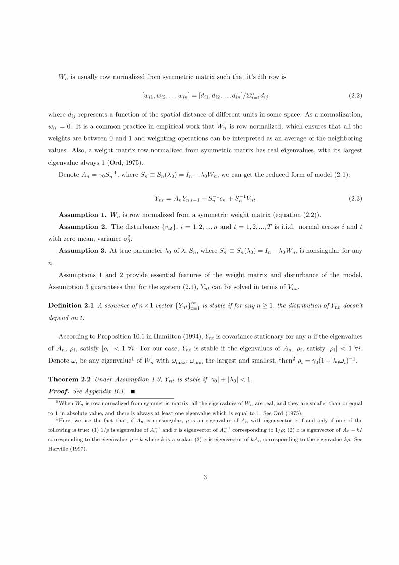
Wn is usually row normalized from symmetric matrix such that it’s ith row is

[wi1, wi2, ..., win] = [di1, di2, ..., din]/Σnj=1dij (2.2)

where dij represents a function of the spatial distance of different units in some space. As a normalization,

wii = 0. It is a common practice in empirical work that Wn is row normalized, which ensures that all the

weights are between 0 and 1 and weighting operations can be interpreted as an average of the neighboring

values. Also, a weight matrix row normalized from symmetric matrix has real eigenvalues, with its largest

eigenvalue always 1 (Ord, 1975).

Denote An = γ0S−1n , where Sn ≡ Sn(λ0) = In − λ0Wn, we can get the reduced form of model (2.1):

Ynt = AnYn,t−1 + S−1n cn + S−1

n Vnt (2.3)

Assumption 1. Wn is row normalized from a symmetric weight matrix (equation (2.2)).

Assumption 2. The disturbance {vit}, i = 1, 2, ..., n and t = 1, 2, ..., T is i.i.d. normal across i and t

with zero mean, variance σ20 .

Assumption 3. At true parameter λ0 of λ, Sn, where Sn ≡ Sn(λ0) = In−λ0Wn, is nonsingular for any

n.

Assumptions 1 and 2 provide essential features of the weight matrix and disturbance of the model.

Assumption 3 guarantees that for the system (2.1), Ynt can be solved in terms of Vnt.

Definition 2.1 A sequence of n×1 vector {Ynt}∞t=1 is stable if for any n ≥ 1, the distribution of Ynt doesn’t

depend on t.

According to Proposition 10.1 in Hamilton (1994), Ynt is covariance stationary for any n if the eigenvalues

of An, ρi, satisfy |ρi| < 1 ∀i. For our case, Ynt is stable if the eigenvalues of An, ρi, satisfy |ρi| < 1 ∀i.

Denote ωi be any eigenvalue1 of Wn with ωmax, ωmin the largest and smallest, then2 ρi = γ0(1− λ0ωi)−1.

Theorem 2.2 Under Assumption 1-3, Ynt is stable if |γ0|+ |λ0| < 1.

Proof. See Appendix B.1.1When Wn is row normalized from symmetric matrix, all the eigenvalues of Wn are real, and they are smaller than or equal

to 1 in absolute value, and there is always at least one eigenvalue which is equal to 1. See Ord (1975).2Here, we use the fact that, if An is nonsingular, ρ is an eigenvalue of An with eigenvector x if and only if one of the

following is true: (1) 1/ρ is eigenvalue of A−1n and x is eigenvector of A−1

n corresponding to 1/ρ; (2) x is eigenvector of An − kI

corresponding to the eigenvalue ρ − k where k is a scalar; (3) x is eigenvector of kAn corresponding to the eigenvalue kρ. See

Harville (1997).

3

When |γ0|+ |λ0| < 1, the eigenvalues of An would all lie inside the unit circle so that Ynt is stable, and

Ynt can be rewritten as

Ynt =∞∑

h=0

AhnS−1

n (cn + Vn,t−h) (2.4)

Using An = γ0S−1n ,

γ0Ynt =∞∑

h=0

Ah+1n (cn + Vn,t−h) = µn + Unt (2.5)

where µn ≡∞∑

h=0

Ah+1n cn and Unt =

∞∑h=0

Ah+1n Vn,t−h are n× 1 vectors.

3 MLE For Stable Case (|γ0|+ |λ0| < 1)

In this section, we derived asymptotic properties of concentrated likelihood estimators when |γ0|+|λ0| < 1

so that Ynt is stable.

To provide analysis of MLE for stable case, following conditions are assumed, and they will be used to

derive the properties of the estimators.

Assumption 4. Wn and S−1n are uniformly bounded in row and column sums in n, i.e., max1≤i≤n

n∑j=1

|wij | <

M and max1≤j≤n

n∑i=1

|wij | < M for all n where M < ∞ and doesn’t depend on n.

Assumption 5. {S−1n (λ)} are uniformly bounded in both row and column sums in n, also uniformly in

λ in a compact parameter space Λ. The true parameter λ0 is in the interior of Λ.

Assumption 6. |γ0|+ |λ0| < 1.

Assumption 7.∞∑

h=1

abs(Ahn) is row sum and column sum bounded, where [abs(An)]ij = |An,ij |.

Assumption 4 is originated by Kelejian and Prucha (1998, 2001). The uniform boundedness of Wn and

S−1n is a condition to limit the spatial correlation to a manageable degree. Assumption 5 is needed to deal

with the nonlinearity of ln |S(λ)| as a function of λ in the likelihood function (3.7). Assumption 6 is the

sufficient condition for Ynt to be stable (Theorem 2.2). Assumption 7 is the absolutely summability condition

and row/column sum boundedness condition, which will play an important role in asymptotic properties of

estimators. This assumption is essential for the paper where both T and n go to infinity because it limits

the dependence between both time series and cross-sectional units.

4

3.1 Lemmas for Several Statistics

Rewrite equation (2.5),

γ0Ynt =∞∑

h=0

Ah+1n (cn + Vn,t−h) = µn + Unt (3.1)

where µn ≡∞∑

h=0

Ah+1n cn and Unt =

∞∑h=0

Ah+1n Vn,t−h are n× 1 vectors.

Following are lemmas for asymptotic behavior of 1nT

T∑t=1

(W1Unt)′(W2Unt) and 1√nT

T∑t=1

(W1Un,t−1)′Vnt

where W1 and W2 are n× n matrices with row sum and column sum bounded. When deriving asymptotics,

n, T →∞ simultaneously and T is a function of n.

Denote Ln =∞∑

h=1

AhnA′hn , then it is row sum and column sum bounded implied by Assumption 7. Accord-

ing to Lee (2001a) (Lemma A.9, page 23), 1n trW1 is O(1) for any n× n row sum and column sum bounded

matrix W1. So, 1n trLn, 1

n trW1Ln and 1n trW ′

1LnW2 are all O(1) because multiplication of two row sum and

column sum bounded matrix is still row sum and column sum bounded.3 Also, denote Unt = Unt− Un where

Un = 1T

T∑t=1

Unt and Un,−1 = 1T

T∑t=1

Un,t−1, and similarly denote Ynt = Ynt − Yn and Vnt = Vnt − Vn, then

γ0Ynt = Unt.

Lemma 3.1 Under Assumption 1-7,

1nT

T∑t=1

(W1Unt)′(W2Unt)−σ2

0

ntrW ′

1W2Lnp→ 0 (3.2)

for any row sum and column sum bounded square matrix W1 and W2 when n, T →∞ simultaneously.

Proof. See Appendix B.2

Lemma 3.2 Under Assumption 1-7,√T

nU ′

n,−1W′1Vn −

√n

Tb1,n = op(1) (3.3)

where b1,n = σ20

n trW1An(In −An)−1.

Proof. See Appendix B.33This follows from properties of matrix norms, i.e., ‖AB‖ ≤ ‖A‖ · ‖B‖ and ‖A + B‖ ≤ ‖A‖ + ‖B‖ for any square matrix

A and B where a function ‖·‖ of a square matrix is a matrix norm if, for any square matrix A and B, it satisfies the following

axioms: (1) ‖A‖ ≥ 0, (1.a) ‖A‖ = 0 if and only if A = 0, (2) ‖cA‖ = |c| ‖A‖ for any scalar c, (3) ‖A + B‖ ≤ ‖A‖ + ‖B‖, (4)

submultiplicative, ‖AB‖ ≤ ‖A‖ · ‖B‖.

5

Lemma 3.3 Under Assumption 1-7, for any row sum and column sum bounded n× n matrix W1,

1√nT

T∑t=1

(W1Yn,t−1)′Vnt +√

n

Tb1,n =⇒ N(0, σ2

W1Yn) (3.4)

when n, T →∞ simultaneously, where σ2W1Yn

= limn,T→∞1

nT

T∑t=1

(W1Yn,t−1)′(W1Yn,t−1) exists.


Lemma 3.4 Under Assumption 2 and that Bn is row sum and column sum bounded,

1√nT

T∑t=1

(V ′ntBnVnt − σ2

0trBn) +√

n

Tb2,n =⇒ N(0, σ2

V ′BV ) (3.5)

when n, T →∞ simultaneously, where σ2V ′BV = limn→∞

σ40

n tr(B′nBn + B2

n) exists and b2,n = σ20

n trBn.


Lemma 3.1 will be used to check the identification of the parameters. Lemma 3.2 to 3.4 will be used to

derive the asymptotic distribution of the estimators.

Using Lemma 3.1,

G1,nT ≡ γ20n−1T−1

T∑t=1

Y ′ntYnt =

σ20

ntrLn + op(1) (3.6a)

G2,nT ≡ γ20n−1T−1

T∑t=1

Y ′ntWnAnYnt =

σ20

ntrWnAnLn + op(1) (3.6b)

G3,nT ≡ γ20n−1T−1

T∑t=1

(WnAnYnt)′WnAnYnt =σ2

0

ntrA′nW ′

nWnAnLn + op(1) (3.6c)

So, G1,nTG3,nT−(G2,nT )2

G1,nT= σ2

0n

trLn×tr(A′nW ′

nWnAnLn)−(trWnAnLn)2

trLn+ op(1).

Assumption 8. limn,T→∞G1,nTG3,nT−(G2,nT )2

G1,nTexists and is nonzero.

This assumption is a sufficient condition for global identification of estimators as we will see in Theorem

3.8.

3.2 Concentrated MLE

The likelihood function of (2.1) is

lnLn,T (θ) = −nT

2ln 2π − nT

2lnσ2 + T ln |Sn(λ)| − 1

2σ2

T∑t=1

V ′nt(δ)Vnt(δ) (3.7)

6

where Vnt(δ) = Sn(λ)Ynt − γYn,t−1 − cn and δ = (λ, γ, c′n)′. Thus, Vnt = Vnt(δ0).

The MLE θn,T is the extreme estimator derived from the maximization of (3.7). As we have nonlinearity

of ln |Sn(λ)| in λ and the number of parameters goes to infinity when n goes to infinity, it’s convenient

to concentrate the cn, γ and σ2 out. From (3.7), given λ, as is derived in Appendix C, the concentrated

estimators are

cn,T (λ) =1T

T∑t=1

(Sn(λ)Ynt − γn,T (λ)Yn,t−1) (3.8a)

γn,T (λ) =

[1

nT

T∑t=1

Y ′n,t−1Yn,t−1

]−1 [1

nT

T∑t=1

Y ′n,t−1Sn(λ)Ynt

](3.8b)

σ2n,T (λ) =

1nT

T∑t=1

[Sn(λ)Ynt − γn,T (λ)Yn,t−1

]′ [Sn(λ)Ynt − γn,T (λ)Yn,t−1

](3.8c)

and the concentrated likelihood is

lnLn,T (λ) = −nT

2(ln 2π + 1)− nT

2ln σ2

n,T (λ) + T ln |Sn(λ)| (3.9)

The MLE λn,T maximizes the concentrated likelihood function (3.9), and the MLE of cn, γ and σ2 are

cn,T (λn,T ), γn,T (λn,T ) and σ2n,T (λn,T ) respectively.

Also, we have corresponding Qn,T (λ) = maxγ,c,σ2 E 1nT lnLn,T (θ).

The optimal solution to above problem is :

c∗n,T (λ) = E1T

T∑t=1

(Sn(λ)Ynt − γ∗n,T (λ)Yn,t−1) (3.10a)

γ∗n,T (λ) =

[E

1nT

T∑t=1


]−1 [E

1nT

T∑t=1


](3.10b)

σ∗2n,T (λ) = E1

nT

T∑t=1

(Sn(λ)Ynt − γ∗n,T (λ)Yn,t−1)′(Sn(λ)Ynt − γ∗n,T (λ)Yn,t−1) (3.10c)

So,

Qn,T (λ) = −12(ln 2π + 1)− 1

2lnσ∗2n,T (λ) +

1n

ln |Sn(λ)| (3.11)

3.3 Consistency of the Concentrated MLE

Identification of λ0 can be based on the maximum value of Qn,T (λ). With the identification and the

uniform convergence of 1nT lnLn,T (λ)−Qn,T (λ) to zero on Λ, consistency follows.

7

Claim 3.5 Under Assumption 1-7, 1nT lnLn,T (λ)−Qn,T (λ)

p→ 0 uniformly in λ in any bounded parameter

space Λ.

Proof. See Appendix D.1.

Also,

∂2Qn,T (λ0)/∂λ2 = − 1γ20σ2

0

EG1,nT EG3,nT − (EG2,nT )2

EG1,nT− 1

n(trG′

nGn + trG2n −

2(trGn)2

n) + o(1) (3.12)

derived in Appendix C where Gn ≡ WnS−1n . Let Cn = Gn − trGn

n In, then 1n (trG′

nGn + trG2n −

2(trGn)2

n ) =1n tr(Cn + C ′

n)(Cn + C ′n)′.

Claim 3.6 If limn,T→∞G1,nTG3,nT−(G2,nT )2

G1,nT6= 0 or limn→∞

1n tr(Cn + C ′

n)(Cn + C ′n)′ 6= 0,

limn,T→∞−∂2Qn,T (λ0)/∂λ2 is positive.


Claim 3.5 is the uniform convergence condition and Claim 3.6 is the local identification condition. Com-

bining uniform convergence and local identification, we can get the consistency of MLE estimators.

Theorem 3.7 Under Assumption 1-7 and limn,T→∞−∂2Qn,T (λ0)/∂λ2 is positive, there exist a neighbor-

hood Λ1 of λ0 such that, for any neighborhood Nε(λ0) of λ0 with radius ε,

lim supn,T→∞

[ maxλ∈Λ1\Nε(λ0)

[Qn,T (λ)−Qn,T (λ0)]] < 0

The MLE λn,T derived from the maximization of lnLn,T (λ) with λ ∈ Λ1 is consistent.


Also, we can get the global identification of λ:

Theorem 3.8 Under Assumption 1-8, λ is globally identified and λn,T is consistent.


When limn,T→∞G1,nTG3,nT−(G2,nT )2

G1,nT= 0 so that Assumption 8 doesn’t hold, the global identification can

still be satisfied from following theorem. Denote σ2n(λ) = σ2

0n tr(S′−1

n S′n(λ)Sn(λ)S−1n ),

Theorem 3.9 Under Assumption 1-7, if limn,T→∞G1,nTG3,nT−(G2,nT )2

G1,nT= 0, then λ is globally identified if

1n ln

∣∣σ2n(λ)S−1

n (λ)′S−1n (λ)

∣∣ 6= 1n ln

∣∣σ20S−1′

n S−1n

∣∣ for λ 6= λ0. And λn,T is consistent.


8

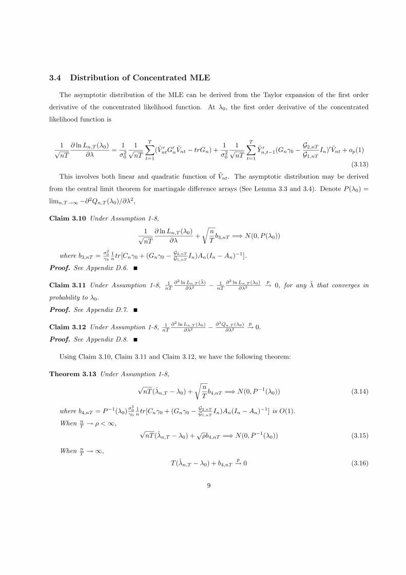
3.4 Distribution of Concentrated MLE

The asymptotic distribution of the MLE can be derived from the Taylor expansion of the first order

derivative of the concentrated likelihood function. At λ0, the first order derivative of the concentrated

likelihood function is

1√nT

∂ lnLn,T (λ0)∂λ

=1σ2

0

1√nT

T∑t=1

(V ′ntG

′nVnt − trGn) +

1σ2

0

1√nT

T∑t=1

Y ′n,t−1(Gnγ0 −

G2,nT

G1,nTIn)′Vnt + op(1)

(3.13)

This involves both linear and quadratic function of Vnt. The asymptotic distribution may be derived

from the central limit theorem for martingale difference arrays (See Lemma 3.3 and 3.4). Denote P (λ0) =

limn,T→∞−∂2Qn,T (λ0)/∂λ2,

Claim 3.10 Under Assumption 1-8,

1√nT


+√

n

Tb3,nT =⇒ N(0, P (λ0))

where b3,nT = σ20

γ0

1n tr[Cnγ0 + (Gnγ0 − G2,nT

G1,nTIn)An(In −An)−1].


Claim 3.11 Under Assumption 1-8, 1nT

∂2 ln Ln,T (λ)∂λ2 − 1

nT∂2 ln Ln,T (λ0)

∂λ2p→ 0, for any λ that converges in

probability to λ0.


Claim 3.12 Under Assumption 1-8, 1nT

∂2 ln Ln,T (λ0)∂λ2 − ∂2Qn,T (λ0)

∂λ2p→ 0.


Using Claim 3.10, Claim 3.11 and Claim 3.12, we have the following theorem:

Theorem 3.13 Under Assumption 1-8,

√nT (λn,T − λ0) +

√n

Tb4,nT =⇒ N(0, P−1(λ0)) (3.14)

where b4,nT = P−1(λ0)σ20

γ0


G1,nTIn)An(In −An)−1] is O(1).

When nT → ρ < ∞,

√nT (λn,T − λ0) +

√ρb4,nT =⇒ N(0, P−1(λ0)) (3.15)

When nT →∞,

T (λn,T − λ0) + b4,nTp→ 0 (3.16)

9


So, from equation (3.14), λn,T is consistent but is biased with the magnitude O( 1T ). The bias results

from the correlation between the averaged error terms and the regressors. As T →∞, the bias will diminish.

For the distribution of λn,T , when n is proportional to T or T is relatively large ( nT → ρ < ∞), λn,T is

asymptotically normal; when n is relatively large ( nT →∞), λn,T will have a degenerate distribution.

After we get the distribution of λn,T , the distribution of γn,T and cn,T can be derived from equation

(3.8).

4 Conclusion

We established the property of MLE of spatial dynamic panel with fixed effects when both T and n

are large. When n is proportional to T or T is relatively large, the estimator is√

nT consistent and

asymptotically normal; when n is relatively large, the estimator is consistent with the rate T and has a

degenerate distribution. The possible contribution of the paper is that it establishes the property of MLE

of spatial dynamic panel when both T and n are large.

Future work could be devoted to (1) introduction of exogenous variables into the model; (2) bias correction

for finite sample; (3) when Ynt is not stable (in progress).

10

Appendices

A Some Useful Lemmas

Let Vnt = (v1t, v2t, · · · , vnt)′ be n × 1 vector and {vit} is i.i.d. across i and t with zero mean, variance

σ20 and finite fourth moment µ4. Denote Unt =

∑∞h=1 PhVn,t+1−h and Wnt =

∑∞h=1 QhVn,t+1−h, where

{Ph}∞h=1 and {Qh}∞h=1 are sequences of n× n nonstochastic square matrix.

Lemma A.1 For t ≥ s,

E(U′ntWns) = σ20tr

( ∞∑h=1

P ′t−s+hQh

)(A.1)

Lemma A.2 For t ≥ s,

Cov(U′ntWnt, U′nsWns) = σ40tr

[( ∞∑h=1

P ′t−s+hQt−s+h

)( ∞∑h=1

PhQ′h +

∞∑h=1

P ′hQh

)](A.2)

+(µ4 − 3σ40)

∞∑g=1

n∑i=1

P ′g,iiQg,ii

Let W1 and W2 are n×n row sum and column sum bounded square matrix and let {Ph}∞h=1 and {Qh}∞h=1

have the form Ph = W1Ph and Qh = W2Q

h. Also, assume∞∑

h=1

abs(Ph) and∞∑

h=1

abs(Qh) are row sum and

column sum bounded where the (i, j) element of abs(Bn) is equal to |Bn,ij |. Denote UnT =(∑T

t=1 Unt

)/T

and Unt = Unt − UnT , also Wnt and Vnt similarly.

Lemma A.3 If W1 and W2 are n×n row sum and column sum bounded square matrix, then W1W2 is also

row sum and column sum bounded.

Theorem A.4 1nT

T∑t=1

U′ntWnt − σ20tr (

∑∞h=1 P ′

hQh)p→ 0 when n, T →∞ simultaneously.4

Theorem A.5 If σ2U = limn→∞

1nσ4

0tr (∑∞

h=1 P ′hPh) exists, 1√

nT

T∑t=1

U′n,t−1Vntd→ N(0, σ2

U) when n, T →∞

simultaneously.

Corollary A.6√

Tn U′nT WnT −

√nT O(1)

p→ 0 when n, T → ∞ simultaneously where the O(1) term is

Tσ20

n tr(∑∞

h=1 PhQ′h

)with Ph = 1

T

h∑g=1

Pg for h ≤ T and Ph = 1T

T∑g=1

Ph−T+g for h > T , and Qh has the

same pattern.4The result also holds either n or T go to infinity only. This also happens to Corrolary A.7.

11

Corollary A.7 1nT

T∑t=1

U′ntWnt − σ20tr (

∑∞h=1 P ′

hQh)p→ 0 when n, T →∞ simultaneously.

Corollary A.8 1√nT

T∑t=1

U′n,t−1Vnt +√

nT

1nσ2

0tr (∑∞

h=1 P ′h) d→ N(0, σ2

U) when n, T →∞ simultaneously.

Proof to Lemma A.1

First, we have the result that EV ′ntW1Vns = trW1 if t = s and EV ′

ntW1Vns = 0 otherwise.

As Unt =∑∞

h=1 PhVn,t+1−h and Wnt =∑∞

h=1 QhVn,t+1−h, using independence of Vnt over t, E(U′ntWns) =

σ20tr(∑∞

h=1 P ′t−s+hQh

).

Proof to Lemma A.2

First, we have the result that5 for E(V ′ntW1Vns)(V ′

ngW2Vnh), it equals

(µ4 − 3σ40)∑n

i=1 W1,iiW2,ii + σ40(trW1 × trW2 + trW1W2 + trW1W

′2) for t = s = g = h

E(V ′ntW1Vns)(V ′

ngW2Vnh) = σ40trW1 × trW2 for t = s 6= g = h

σ40tr(W1W2) for t = g 6= s = h

σ40tr(W1W

′2) for t = h 6= s = g

0 otherwiseE(U′ntWnt × U′nsWns)

= E(∑t−s

h=1 PhVn,t+1−h +∑∞

g=1 Pt−s+gVn,s+1−g)′(∑t−s

h=1 QhVn,t+1−h +∑∞

g=1 Qt−s+gVn,s+1−g)

×(∑∞

g=1 PgVn,s+1−g)′(∑∞

g=1 QgVn,s+1−g)

= E(∑t−s

h=1 PhVn,t+1−h)′(∑t−s

h=1 QhVn,t+1−h)× (∑∞

g=1 PgVn,s+1−g)′(∑∞

g=1 QgVn,s+1−g)

+E(∑∞

g=1 Pt−s+gVn,s+1−g)′(∑∞

g=1 Qt−s+gVn,s+1−g)× (∑∞

g=1 PgVn,s+1−g)′(∑∞

g=1 QgVn,s+1−g)

= E1 + E2

E1 = E(∑t−s

h=1 PhVn,t+1−h)′(∑t−s

h=1 QhVn,t+1−h)× (∑∞

g=1 PgVn,s+1−g)′(∑∞

g=1 QgVn,s+1−g)

= tr(∑t−s

h=1 P ′hQh

)× tr

(∑∞g=1 P ′

gQg

)E2 = E(

∑∞g=1 Pt−s+gVn,s+1−g)′(

∑∞g=1 Qt−s+gVn,s+1−g)× (

∑∞g=1 PgVn,s+1−g)′(

∑∞g=1 QgVn,s+1−g)

= E(∑∞

g=1(Pt−s+gVn,s+1−g)′Qt−s+gVn,s+1−g +∑∞

g=1

∑∞h6=g(Pt−s+hVn,s+1−h)′Qt−s+gVn,s+1−g))

×(∑∞

g=1(PgVn,s+1−g)′QgVn,s+1−g +∑∞

g=1

∑∞h6=g(PhVn,s+1−h)′QgVn,s+1−g))

= E((∑∞

g=1(Pt−s+gVn,s+1−g)′Qt−s+gVn,s+1−g)× (∑∞

g=1(PgVn,s+1−g)′QgVn,s+1−g))

+E((∑∞

g=1

∑∞h6=g(Pt−s+hVn,s+1−h)′Qt−s+gVn,s+1−g)× (

∑∞g=1

∑∞h6=g(PhVn,s+1−h)′QgVn,s+1−g)

)= E21 + E22

5In Lee (2001a), Lemma A.10 in his paper is the result for E(V ′ntW1Vnt)2. It can easily extended to

E(V ′ntW1Vns)(V ′

ngW2Vnh).

12

E21 = E(∑∞

g=1(Pt−s+gVn,s+1−g)′Qt−s+gVn,s+1−g(PgVn,s+1−g)′QgVn,s+1−g

)+E

(∑∞g=1

∑∞h6=g(Pt−s+hVn,s+1−h)′Qt−s+hVn,s+1−h(PgVn,s+1−g)′QgVn,s+1−g

)= (µ4 − 3σ4

0)∑∞

g=1

∑ni=1 P ′

g,iiQg,ii

+σ40

∑∞g=1 tr(P ′

t−s+gQt−s+g)×tr(P ′gQg)+σ4

0

∑∞g=1 tr(P ′

t−s+gQt−s+gP′gQg)+σ4

0

∑∞g=1 tr(P ′

t−s+gQt−s+gPgQ′g)

+σ40

(∑∞g=1 tr(P ′

t−s+gQt−s+g))∑∞

g=1 tr(P ′gQg)− σ4

0

∑∞g=1 tr(P ′

t−s+gQt−s+g)× tr(P ′gQg)

= σ40

∑∞g=1 tr(P ′

t−s+gQt−s+g)tr(P ′gQg) + σ4

0

∑∞g=1 tr(P ′

t−s+gQt−s+gPgQ′g)

+σ40

(∑∞g=1 tr(P ′


g=1 tr(P ′gQg)

E22 = E(∑∞

g=1

∑∞h6=g(Pt−s+hVn,s+1−h)′Qt−s+gVn,s+1−g)× (

∑∞g=1

∑∞h6=g(PhVn,s+1−h)′QgVn,s+1−g))

= σ40tr[(∑∞

h=1 P ′t−s+hQt−s+h

)∑∞h=1 PhQ′

h

]− σ4

0tr[(∑∞


)PhQ′

h

]+σ4

0tr[(∑∞


)∑∞h=1 P ′

hQh

]− σ4

0tr[(∑∞


)P ′

hQh

]So, E2 = E21 + E22 = (µ4 − 3σ4

0)∑∞

g=1

∑ni=1 P ′

g,iiQg,ii+

σ40

(∑∞g=1 tr(P ′


g=1 tr(P ′gQg)+σ4

0tr[(∑∞


)(∑∞

h=1 PhQ′h +

∑∞h=1 P ′

hQh)]

As Cov(U′ntWnt, U′nsWns) = E(U′ntWnt × U′nsWns)− EU′ntWnt × EU′nsWns,

Cov(U′ntWnt, U′nsWns) = E1 + E2 − σ40tr (

∑∞h=1 P ′

hQh) tr (∑∞

h=1 P ′hQh)

= (µ4 − 3σ40)∑∞

g=1

∑ni=1 P ′

g,iiQg,ii + σ40tr[(∑∞


)(∑∞

h=1 PhQ′h +

∑∞h=1 P ′

hQh)].

Proof to Lemma A.3

This is Lemma A.1 in Lee (2003).

Proof for Theorem A.4

We use Chebyshev’s inequality to prove the law of large numbers.

First, Lemma A.1 states that E(U′ntWns) = σ20tr

( ∞∑h=1

P ′hQh

)for t ≥ s, then, E 1

nT

T∑t=1

U′ntWnt =

1nσ2

0tr

( ∞∑h=1

P ′hQh

).

Second, Lemma A.2 states that Cov(U′ntWnt, U′nsWns) = σ40tr

[( ∞∑h=1

P ′t−s+hQt−s+h

)( ∞∑h=1

PhQ′h +

∞∑h=1

P ′hQh

)]+

(µ4 − 3σ40)∑∞

g=1

∑ni=1 P ′

g,iiQg,ii for t ≥ s.

So, V ar(T∑

t=1U′ntWnt) =

T∑t=1

T∑s=1

Cov(U′ntWnt, U′nsWns)

= σ40tr

[(T∑

t=1

T∑s=1

∞∑h=1

P ′|t−s|+hQ|t−s|+h

)( ∞∑h=1

PhQ′h +

∞∑h=1

P ′hQh

)]+ (µ4 − 3σ4

0)∑∞

g=1

∑ni=1 P ′

g,iiQg,ii

As Ph = W1Ph and Qh = W2Q

h and∞∑

h=1

abs(Ph) and∞∑

h=1

abs(Qh) row sum and column sum bounded,

using Lemma A.3, 1nT var(

T∑t=1

U′ntWnt) < σ40M where M < ∞, so that V ar( 1

nT

T∑t=1

U′ntWnt) → 0.

13

Proof for Theorem A.5

We will use the CLT for dependent array in Davidson (1994) (Theorem 24.1, page 380) to establish

our CLT, our proof is similar to the proof of Theorem 24.3 in Davidson (1994). In his proof, following 2

theorems are used (Theorem 24.1 and Theorem 24.2).

Theorem 24.1 Let {Znt, t = 1, ..., rn, n ∈ N} denote a zero-mean stochastic array, where rn is a positive,

increasing integer-valued function of n, and let

Trn=

rn∏t=1

(1 + iλZnt), λ > 0 (A.3)

Then, Srn =∑rn

t=1 ZntD→ N(0, 1) if the following conditions hold:

(a) Trnis uniformly integrable,

(b) E(Trn) → 1 as n →∞,

(c)∑rn

t=1 Z2nt

pr→ 1 as n →∞,

(d) max1≤t≤rn |Znt|pr→ 0 as n →∞.

Theorem 24.2 For an array {Znt}, let

Znt = Znt1(∑t−1

k=1Z2

nk ≤ 2) (A.4)

(i) The sequence Trn =rn∏t=1

(1 + iλZnt) is uniformly integrable if

supn

E

(max

1≤t≤rn

Z2nt

)< ∞. (A.5)

And if∑rn

t=1 Z2nt

pr→ 1, then

(ii)∑rn

t=1 Z2nt

pr→ 1;

(iii)Srn=∑rn

t=1 Znt has the same limiting distribution as Srn.

In our case, we are going to check the CLT of 1√nT

rn∑t=1

U′n,t−1Vnt with t = 1, .., rn, where T is a function

of n, with rn = T .

Assume that σ2U,nT ≡ E 1

nT

T∑t=1

U′n,t−1Un,t−1 and σ2U ≡ limn,T→∞E 1

nT

T∑t=1

U′n,t−1Un,t−1 = limn→∞σ20

n tr (∑∞

h=1 P ′hPh)

exists, then, define SnT =T∑

t=1Znt where Znt = 1√

nTσ2U,nT

U′n,t−1Vnt.

σ2nt ≡ V ar(Znt) = 1

nTσ2U,nT

V ar(U′n,t−1Vnt) = σ20

nTσ2U,nT

E(U′n,t−1Un,t−1) and we can get

∑T

t=1σ2

nt = 1 (A.6)

14

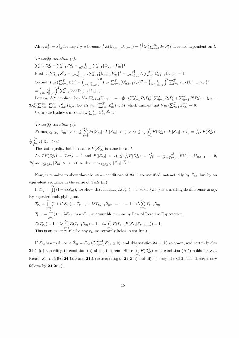
Also, σ2nt = σ2

ns for any t 6= s because 1nE(U′n,t−1Un,t−1) = σ2

0n tr (

∑∞h=1 PhP ′

h) does not dependent on t.

To verify condition (c):∑rn

t=1 Z2nt =

∑Tt=1 Z2

nt = 1nTσ2

U,nT

∑Tt=1{U′n,t−1Vnt}2

First, E∑T

t=1 Z2nt = 1

nTσ2U,nT

E∑T

t=1{U′n,t−1Vnt}2 = σ20

nTσ2U,nT

E∑T

t=1 U′n,t−1Un,t−1 = 1.

Second, V ar(∑T

t=1 Z2nt) =

(1

nTσ2U,nT

)2

V ar∑T

t=1{U′n,t−1Vnt}2 =(

1nTσ2

U,nT

)2∑Tt=1 V ar{U′n,t−1Vnt}2

=(

σ20

nTσ2U,nT

)2∑Tt=1 V arU′n,t−1Un,t−1

Lemma A.2 implies that V arU′n,t−1Un,t−1 = σ40tr (

∑∞h=1 PhP ′

h) (∑∞

h=1 PhP ′h +

∑∞h=1 P ′

hPh) + (µ4 −

3σ40)∑∞

h=1

∑ni=1 P ′

h,iiPh,ii. So, nTV ar(∑T

t=1 Z2nt) < M which implies that V ar(

∑Tt=1 Z2

nt) → 0.

Using Chebyshev’s inequality,∑T

t=1 Z2nt

p→ 1.

To verify condition (d):

P (max1≤t≤rn|Znt| > ε) ≤

rn∑t=1

P (|Znt| · I(|Znt| > ε) > ε) ≤ 1ε2

rn∑t=1

E(Z2nt) · I(|Znt| > ε) = 1

ε2 TE(Z2nt) ·

1T

rn∑t=1

I(|Znt| > ε)

The last equality holds because E(Z2nt) is same for all t.

As TE(Z2nt) = Tσ2

nt = 1 and P (|Znt| > ε) ≤ 1ε2 E(Z2

nt) = σ2nt

ε2 = 1ε2

σ20

nTσ2U,nT

EU′n,t−1Un,t−1 → 0,

P (max1≤t≤rn|Znt| > ε) → 0 so that max1≤t≤rn

|Znt|pr→ 0.

Now, it remains to show that the other conditions of 24.1 are satisfied; not actually by Znt, but by an

equivalent sequence in the sense of 24.2 (iii).

If Trn=

rn∏t=1

(1 + iλZnt), we show that limn→∞E(Trn) = 1 when {Znt} is a martingale difference array.

By repeated multiplying out,

Trn=

rn∏t=1

(1 + iλZnt) = Trn−1 + iλTrn−1Znrn= · · · = 1 + iλ

rn∑t=1

Tt−1Znt.

Tt−1 =t∏

s=1(1 + iλZns) is a Ft−1-measurable r.v., so by Law of Iterative Expectation,

E(Trn) = 1 + iλrn∑t=1

E(Tt−1Znt) = 1 + iλrn∑t=1

E(Tt−1E(Znt|Frn,t−1)) = 1.

This is an exact result for any rn, so certainly holds in the limit.

If Znt is a m.d., so is Znt = Znt1(∑t−1

k=1 Z2nk ≤ 2), and this satisfies 24.1 (b) as above, and certainly also

24.1 (d) according to condition (b) of the theorem. SinceT∑

t=1E(Z2

nt) = 1, condition (A.5) holds for Znt.

Hence, Znt satisfies 24.1(a) and 24.1 (c) according to 24.2 (i) and (ii), so obeys the CLT. The theorem now

follows by 24.2(iii).

15

So,1√nT

T∑t=1

U′n,t−1Vnt =⇒ N(0, σ2U) (A.7)

Proof for Corollary A.6

Let UnT = UnT and WnT = WnT , then UnT =∑∞

h=1 PhVT+1−h and WnT =∑T

h=1 QhVT+1−h where

Ph = 1T (P1 + P2 + · · ·+ Ph) = 1

T

h∑g=1


T∑g=1

Ph−T+g for h > T , and Qh has the same

pattern.

First, using Lemma A.1, EU′nT WnT = EU′nT WnT = σ20tr(∑∞

h=1 PhQ′h

).


h, Ph = 1T W1

h∑g=1

P g for h ≤ T and Ph = 1T W1

T∑g=1

Ph−T+g for h > T .

Also,∞∑

h=1

abs(Ph) and∞∑

h=1

abs(Qh) row sum and column sum bounded, using Lemma A.3, tr(∑∞

h=1 PhQ′h

)is O( n

T ).

So, E√

Tn U′nT WnT =σ2

0

√Tn tr

(∑∞h=1 P ′

hQh

)=√

nT

σ20

n tr(T∑∞

h=1 P ′hQh

)which is

√nT O(1).

Second, using Lemma A.2, V ar(√

Tn U′nT WnT ) = T

n varU′nT WnT = Tn Cov(U′nT WnT , U′nT WnT )

= σ40tr[(∑∞

h=1 P ′hQh

)(∑∞h=1 P ′

hQh +∑∞

h=1 PhQ′h

)]+ (µ4 − 3σ4

0)∑∞

h=1

∑ni=1 P ′

h,iiQh,ii.

Here, Ph = 1T (P1 + P2 + · · ·+ Ph) = 1

T

h∑g=1


T∑g=1

Ph−T+g for h > T .


h and∞∑

h=1

abs(Ph) and∞∑

h=1

abs(Qh) row sum and column sum bounded,

using Lemma A.3, V ar( 1n U′nT WnT ) = O( 1

T ) → 0.

So,√

Tn U′nT WnT −

√nT O(1)

p→ 0 where the O(1) term is Tσ20

n tr(∑∞

h=1 PhQ′h

).

Proof for Corollary A.71

nT

T∑t=1

U′ntWnt = 1nT

T∑t=1

U′ntWnt− 1n U′nT WnT . Using Theorem A.4 and Corollary A.6, the result follows.

Proof for Corollary A.81√nT

T∑t=1

U′n,t−1Vnt = 1√nT

T∑t=1

U′n,t−1Vnt−√

Tn U′nT VnT . Using Theorem A.5 and Corollary A.6, the result

follows.

B Proofs For Theorems and Lemmas

B.1 Proof of Theorem 2.2

If all the eigenvalues of An are smaller than one in magnitude, as vit is i.i.d., Ynt is stable. So, to

prove stability, we need to prove that all the eigenvalues of An are smaller than one in magnitude when

|γ0|+ |λ0| < 1.

16

An = γ0(In − λ0Wn)−1, so the eigenvalue of An is ρi = γ0(1− λ0ωi)−1 where ωi is any eigenvalue of the

weight matrix Wn,

|ρi| < 1 ⇐⇒∣∣γ0(1− λ0ωi)−1

∣∣ < 1 ⇐⇒ |γ0| < |1− λ0ωi|

When Wn is row normalized6, ωmax = 1.

(1)If 0 < λ0 < 1, then |γ0| < 1− λ0ωi ∀i ⇐⇒ ωi < 1−|γ0|λ0

∀i ⇐⇒ ωmax < 1−|γ0|λ0

⇐⇒ |γ0|+ λ0 < 1.

(2)If −1 < λ0 < 0, then |γ0| < 1 − λ0ωi ∀i ⇐⇒ ωi > − 1−|γ0||λ0| ∀i ⇐⇒ ωmin > − 1−|γ0|

|λ0| ⇐⇒

|γ0|+ λ0ωmin < 1 ⇐= |γ0|+ |λ0| < 1.

(3)If λ0 = 0, then |γ0| < |1− λ0ωi| ⇐⇒ |γ0| < 1.

To sum up, |γ0| + |λ0| < 1 =⇒ the eigenvalues of An all lie inside the unit circle =⇒ Ynt is covariance

stationary.

With Vnt being iid here, Ynt is also strictly stationary, which is stable according to definition 2.1.

B.2 Proof for Lemma 3.1

Using Corollary A.7, we can get the result. Here, Ph = W1Ahn and Qn = W2A

hn. So, tr (

∑∞h=1 P ′

hQh) =

tr(∑∞

h=1 A′hn W ′1W2A

hn

)= tr

(W ′

1W2

∑∞h=1 Ah

nA′hn)

= tr (W ′1W2Ln).


Using Corollary A.6, we can get the result. Here, Ph = W1Ahn and Qh = In so that Ph = 1

T W1

h∑g=1

Agn

for h ≤ T and Ph = 1T W1

T∑g=1

Ah−T+gn for h > T and Qh = 1

T In for all h. So, Tn tr

(∑∞h=1 PhQ′

h

)=

1n tr

(W1An(In −An)−1

)+ o(1).


Using Corollary A.8, we have the result. Here, Un,t−1 = W1Yn,t−1 with Ph = W1Ahn.


Corollary A.8 is the CLT for martingale difference arrays, which certainly holds for independent arrays.6When Wn is row normalized from symmetric matrix, all the eigenvalues of Wn are real, and they are smaller than or equal

to 1 in absolute value, and there is always at least one eigenvalue which is equal to 1. See Ord (1975).

17

C Concentrated MLE

The likelihood function for (2.1) is

lnLn,T (θ) = −nT

2ln 2π − nT

2lnσ2 + T ln |Sn(λ)| − 1

2σ2

T∑t=1

V ′nt(δ)Vnt(δ) (C.1)

where Vt(δ) = Sn(λ)Ynt − γYn,t−1 − cn and δ = (λ, γ, c′n)′.

The FOCs are

∂ lnLn,T (θ)∂γ

=1σ2

T∑t=1

Y ′n,t−1Vnt(δ) (C.2a)

∂ lnLn,T (θ)∂λ

=1σ2

T∑t=1

(WnYnt)′Vnt(δ)− TtrGn(λ) (C.2b)

∂ lnLn,T (θ)∂cn

=1σ2

T∑t=1

Vnt(δ) (C.2c)

∂ lnLn,T (θ)∂σ2

= − nT

2σ2+

12σ4

T∑t=1

V ′nt(δ)Vnt(δ) (C.2d)

where Gn(λ) = WnS−1n (λ).

C.1 Concentrated Estimators

Denote Ynt = Ynt − Yn, given λ, we can get

cn,T (λ) =1T

T∑t=1

(Sn(λ)Ynt − γn,T (λ)Yn,t−1) (C.3a)

γn,T (λ) =

[1

nT

T∑t=1


]−1 [1

nT

T∑t=1


](C.3b)

σ2n,T (λ) =

1nT

T∑t=1

(Sn(λ)Ynt − γn,T (λ)Yn,t−1)′(Sn(λ)Ynt − γn,T (λ)Yn,t−1) (C.3c)

So, the concentrated likelihood is

lnLn,T (λ) = −nT

2(ln 2π + 1)− nT

2ln σ2

n,T (λ) + T ln |Sn(λ)| (C.4)

Also, we have corresponding Qn,T (λ) = maxγ,c,σ2 E 1nT lnLn,T (θ).

The optimal solution to above problem is :

18

c∗n,T (λ) = E1T

T∑t=1

(Sn(λ)Ynt − γ∗n,T (λ)Yn,t−1) (C.5)

γ∗n,T (λ) =[E

1nT


]−1[E

1nT

T∑t=1


](C.6)

σ∗2n,T (λ) = E1

nT

T∑t=1

(Sn(λ)Ynt − γ∗n,T (λ)Yn,t−1)′(Sn(λ)Ynt − γ∗n,T (λ)Yn,t−1) (C.7)

So,

Qn,T (λ) = −12(ln 2π + 1)− 1

2lnσ∗2n,T (λ) +

1n

ln |Sn(λ)| (C.8)

Using Ynt = S−1n Yn,t−1γ0 + S−1

n Vnt and Sn(λ)S−1n = In + (λ0−λ)Gn where Gn = WnS−1

n ,from equation

(C.3),

γn,T (λ) = γ0 − (λ− λ0)G2,nT

G1,nT+

γ20

G1,nT

[1

nT

T∑t=1

Y ′n,t−1Sn(λ)S−1

n Vnt

](C.9)

σ2n,T (λ) = (λ− λ0)2

G1,nTG3,nT − G22,nT

γ20G1,nT

+1

nT

T∑t=1

V ′ntS

′−1n S′n(λ)Sn(λ)S−1

n Vnt (C.10)

+2(λ0 − λ)1

nT

T∑t=1


G2,nT

G1,nTIn)′Sn(λ)S−1

n Vnt

− γ20

G1,nT(

1nT

T∑t=1


n Vnt)2

Also, (C.10) implies that

∂σ2n,T (λ)∂λ

= 2(λ− λ0)G1,nTG3,nT − G2

2,nT

γ20G1,nT

− 2nT

T∑t=1

V ′ntG

′nSn(λ)S−1

n Vnt (C.11)

−2(λ0 − λ)1

nT

T∑t=1


G2,nT

G1,nTIn)′GnVnt

− 2nT

T∑t=1


G2,nT

G1,nTIn)′Sn(λ)S−1

n Vnt

+2γ2

0

G1,nT(

1nT

T∑t=1


n Vnt)1

nT

T∑t=1

Y ′n,t−1GnVnt

19

∂2σ2n,T (λ)∂λ2

= 2G1,nTG3,nT − G2

2,nT

γ20G1,nT

+2

nT

T∑t=1

V ′ntG

′nGnVnt (C.12)

+4

nT

T∑t=1


G2,nT

G1,nTIn)′GnVnt

− 2γ20

G1,nT(

1nT

T∑t=1

Y ′n,t−1GnVnt)2

We have 1nT

T∑t=1

Y ′n,t−1W1Vnt

p→ 0 implied by Corollary A.7 for any row sum and column sum bounded

matrix W1, so,

σ2n,T (λ) = (λ− λ0)2


γ20G1,nT

+ σ20

1n

tr(S′−1n S′n(λ)Sn(λ)S−1

n ) + op(1) (C.13a)

√nT

∂σ2n,T (λ0)∂λ

= − 2√nT

T∑t=1

V ′ntG

′nVnt −

2√nT

T∑t=1


G2,nT

G1,nTIn)′Vnt + op(1) (C.13b)

∂2σ2n,T (λ)∂λ2

= 2G1,nTG3,nT − G2

2,nT

γ20G1,nT

+ 2σ20

1n

trG′nGn + op(1) (C.13c)

Also,

σ∗2n,T (λ) = (λ− λ0)2EG1,nT EG3,nT − EG2

2,nT

γ20EG1,nT

+ σ20

1n


n ) + o(1) (C.14a)

∂σ∗2n,T (λ0)∂λ

= −2E1

nT

T∑t=1

V ′ntG

′nVnt + o(1) (C.14b)

∂2σ∗2n,T (λ)∂λ2

= 2EG1,nT EG3,nT − (EG2,nT )2

γ20EG1,nT

+ 2σ20

1n

trG′nGn + o(1) (C.14c)

C.2 The FOC and SOC of Concentrated MLE

From concentrated likelihood function (C.4),

1nT

∂ lnLn,T (λ)∂λ

= − 12σ2

n,T (λ)∂σ2

n,T (λ)∂λ

− 1n

trGn(λ) (C.15)

1nT

∂2 lnLn,T (λ)∂λ2

= − 12σ4

n,T (λ)

[∂2σ2

n,T (λ)∂λ2

σ2n,T (λ)− (

∂σ2n,T (λ)∂λ

)2]− 1

ntr(G2

n(λ)) (C.16)

Using equation (C.13),

20

1nT

∂2 lnLn,T (λ0)∂λ2

= − 1γ20σ2

0


G1,nT− 1

n(trG′

nGn + trG2n −

2(trGn)2

n) + op(1) (C.17)

Using equation (C.13), according to Lemma 3.3 and 3.4,

1√nT


+√

n

TO(1) =⇒ N(0, P (λ0)) (C.18)

where P (λ0) = 1γ20σ2

0limn,T→∞

G1,nTG3,nT−(G2,nT )2

G1,nT+ limn→∞

1n trC ′

nCn, Cn = Gn − trGn

n In and the O(1)

term is σ20

γ0


G1,nTIn)An(In −An)−1]

Similarly, from equation (C.14),

∂Qn,T (λ0)∂λ

p→ 0 (C.19)

∂2Qn,T (λ0)/∂λ2 = − 1γ20σ2

0


EG1,nT− 1

n(trG′

nGn + trG2n −

2(trGn)2

n) + o(1) (C.20)

D Proofs For Consistency and asymptotic normality

D.1 Proof of Claim 3.5

As lnLn,T (λ) = −nT2 (ln 2π+1)− nT

2 ln σ2n,T (λ)+T ln |Sn(λ)| and Qn,T (λ) = − 1

2 (ln 2π+1)− 12 lnσ∗2n,T (λ)+

1n ln |Sn(λ)| (equation (3.9) and (3.11)), 1

nT lnLn,T (λ)−Qn,T (λ) = 12 lnσ∗2n,T (λ)− 1

2 ln σ2n,T (λ).

By mean value theorem,

1nT

lnLn,T (λ)−Qn,T (λ) = −12

1σ2

n,T (λ)(σ2

n,T (λ)− σ∗2n,T (λ)) (D.1)

where σ2n,T (λ) lies between σ2

n,T (λ) and σ∗2n,T (λ).

We need to show that (1) σ2n,T (λ)− σ∗2n,T (λ) → 0 uniformly and (2) σ2

n,T (λ) is uniformly bounded away

from zero.

(1):

From equation (C.13) and (C.14),

σ2n,T (λ) = (λ− λ0)2

G1,nTG3,nT−G22,nT

γ20G1,nT

+ σ20

1n tr(S′−1

n S′n(λ)Sn(λ)S−1n ) + op(1)

σ∗2n,T (λ) = (λ− λ0)2EG1,nT EG3,nT−EG2

2,nT

γ20EG1,nT

+ σ20

1n tr(S′−1

n S′n(λ)Sn(λ)S−1n ) + o(1).

According to equation (3.6) and Lemma 3.1, G1,nTG3,nT−G22,nT

G1,nT− EG1,nT EG3,nT−(EG2,nT )2

EG1,nT

p→ 0. So, we can

get σ2n,T (λ)− σ∗2n,T (λ) → 0.

21

(2):

σ2n,T (λ) lies between σ2

n,T (λ) and σ∗2n,T (λ), 1σ2

n,T (λ)≤ 1

σ2n,T (λ)

+ 1σ∗2n,T (λ)

.

Denote σ2n,T (λ) = σ2

01n tr(S′−1

n S′n(λ)Sn(λ)S−1n ), then σ2

n,T (λ) is uniformly bounded away from zero7. AsG1,nTG3,nT−G2

2,nT

G1,nTis nonnegative8, σ2

n,T (λ) and σ∗2n,T (λ) are uniformly bounded away from zero. So, 1σ2

n,T (λ)is

uniformly bounded.

Combining σ2n,T (λ) − σ∗2n,T (λ) → 0 and 1

σ2n,T (λ)

uniformly bounded in λ, 1nT lnLn,T (λ) − Qn,T (λ)

p→ 0

uniformly in λ.


We have equation (C.20):

∂2Qn,T (λ0)/∂λ2 = − 1γ20σ2

0


EG1,nT− 1

n(trG′

nGn + trG2n −

2(trGn)2

n) + o(1)

then, limn,T→∞∂2Qn,T (λ0)

∂λ2 = − 1γ20σ2

0limn,T→∞


G1,nT−limn→∞

σ20

n [trG′nGn+trG2

n−2(trGn)2

n ]

If limn,T→∞G1,nTG3,nT−(G2,nT )2

G1,nT6= 0 or limn→∞

1n (trG′

nGn + trG2n−

2(trGn)2

n ) 6= 0, limn,T→∞−∂2Qn,T (λ0)∂λ2

is positive.

Here, G1,nTG3,nT−(G2,nT )2

G1,nT≥ 0 because of the Cauchy inequality shown in Appendix D.1; also,denote

Cn = Gn − trGn

n In, then, 1n{trG

′nGn + trG2

n −2(trGn)2

n } = 1n tr(Cn + C ′

n)(Cn + C ′n)′ ≥ 0.

D.3 Proof of Theorem 3.7

Using positiveness of limn,T→∞−∂2Qn,T (λ0)∂λ2 , we can first get that the identification uniqueness holds

on Λ1, a neighborhood of λ0. Then using uniform convergence and identification uniqueness, we can get

consistency.

We expand Qn,T (λ) around λ0 : Qn,T (λ) = Qn,T (λ0) + ∂Qn,T (λ0)∂λ (λ− λ0) + 1

2∂2Qn,T (λ)

∂λ2 (λ− λ0)2 where λ

lies between λ and λ0.7See the supplement to Lee (2204) , Page 8 for the proof of consistency, available in http://economics.sbs.ohio-state.edu/lee/.

8Here,G1,nT G3,nT−(G2,nT )2

G1,nT≥ 0 because of the Cauchy inequality: G1,nT = γ2n−1T−1

TPt=1

Y ′ntYnt = γ2n−1T−1

TPt=1

nPi=1

a2it,

G2,nT = γ2n−1T−1TP

t=1Y ′

ntWnAnYnt = γ2n−1T−1TP

t=1

nPi=1

aitbit and G3,nT = γ2n−1T−1TP

t=1(WnAnYnt)′WnAnYnt =

γ2n−1T−1TP

t=1

nPi=1

b2it where ait = (Ynt)i and bit = (WnYnt)i. Then,

TP

t=1

nPi=1

a2it

! TP

t=1

nPi=1

b2it

!−

TPt=1

nPi=1

aitbit

!2

≥ 0.

The equality holds only when ait = bit, which means Ynt = WnYnt for all t.

22

At λ = λ0,∂Qn,T (λ0)

∂λ = o(1) (equation (C.19)) and ∂2Qn,T (λ0)∂λ2 = − 1

γ20σ2

0

EG1,nT EG3,nT−(EG2,nT )2

EG1,nT− 1

n [trG′nGn+

trG2n −

2(trGn)2

n ] + o(1) (equation (C.20)), so for Taylor expansion, Qn,T (λ) − Qn,T (λ0) = 12

∂2Qn,T (λ)∂λ2 (λ −

λ0)2 + o(1) where λ lies between λ and λ0.

So, Qn,T (λ)−Qn,T (λ0) = 12 (λ−λ0)2 limn,T→∞

∂2Qn,T (λ0)∂λ2 + 1

2 (λ−λ0)2[∂2Qn,T (λ)

∂λ2 −limn,T→∞∂2Qn,T (λ0)

∂λ2 ]+

o(1).

As limn,T→∞−∂2Qn,T (λ0)∂λ2 is positive from Claim 3.6, there exist a constant c > 0 such that 1

2 (λ −

λ0)2 limn,T→∞∂2Qn,T (λ0)

∂λ2 < −c.

As tr[(WnS−1n (λ))2]−tr(G2

n) = 2n tr[(WnS−1

n (λ))3](λ−λ0) where λ lies between λ and λ0, and 1n tr[(WnS−1

n (λ))3]

is uniformly bounded (see Lemma A.8 in Lee (2001a)), it follows that9 ∂2Qn,T (λ)∂λ2 − limn,T→∞

∂2Qn,T (λ0)∂λ2 = 0

whenever λ → λ0. So, there exist a neighbor Λ1 of λ0 such that supλ∈Λ1

∣∣∣∂2Qn,T (λ)∂λ2 − limn,T→∞

∂2Qn,T (λ0)∂λ2

∣∣∣ ≤c/2. Hence,

Qn,T (λ)−Qn,T (λ0) ≤ 12 (λ− λ0)2 limn,T→∞

∂2Qn,T (λ0)∂λ2 + c

4 (λ− λ0)2 < − c4 (λ− λ0)2,

that is, the identification uniqueness property holds on Λ1. The consistency then comes from the identi-

fication uniqueness and that 1nT lnLn,T (λ)−Qn,T (λ)

p→ 0 uniformly in Claim 3.5. (See White (1994)).


We have Qn,T (λ) = − 12 (ln 2π + 1)− 1

2 lnσ∗2n,T (λ) + 1n ln |Sn(λ)| where

σ∗2n,T (λ) = (λ0 − λ)2 EG1,nT EG3,nT−(EG2,nT )2

EG1,nT+ 1

nσ20tr(S′−1

n Sn(λ)Sn(λ)S−1n ) + o(1).

At λ = λ0, Qn,T (λ0) = − 12 (ln 2π + 1)− 1

2 lnσ∗2n,T (λ0) + 1n ln |Sn(λ0)|.

We are going to prove that Qn,T (λ) < Qn,T (λ0) for any λ 6= λ0.

Qn,T (λ)−Qn,T (λ0) = − 12 [lnσ∗2n,T (λ)− lnσ∗2n,T (λ0)] + 1

n ln |Sn(λ)| − 1n ln |Sn(λ0)|

= T1 − T2 where

T1 = − 12 [ln{ 1

nσ20tr(S′−1

n Sn(λ)Sn(λ)S−1n )} − lnσ∗2(λ0)] + 1

n ln |Sn(λ)| − 1n ln |Sn(λ0)| and

T2 = ln(1 +(λ0−λ)2

EG1,nT EG3,nT−(EG2,nT )2

γ20EG1,nT

1n σ2

0tr(S′−1n Sn(λ)Sn(λ)S−1

n )).

Consider the pure spatial dynamic panel process Ynt = λ0WnYnt+cn+Vnt, the concentrated log likelihood

function of this process is

lnLp,n,T (θ) = −nT

2ln 2π − nT

2lnσ2 + T ln |Sn(λ)| − 1

2σ2

T∑t=1

(Sn(λ)Ynt − cn)′(Sn(λ)Ynt − cn) (D.2)

9Using ∂2Qn,T (λ)/∂λ2 = − 12σ∗2

n,T(λ)

[∂2σ∗2n,T (λ)

∂λ2 σ∗2n,T (λ)− (∂σ∗2n,T (λ)

∂λ)2]− 1

ntr(G2

n(λ)) and equation (C.14).

23

And the concentrated likelihood is

lnLp,n,T (λ) = −nT

2(ln 2π + 1)− nT

2ln σ2

p,n,T (λ) + T ln |Sn(λ)| (D.3)

where

cp,n,T (λ) =1T

T∑t=1

Sn(λ)Ynt (D.4)

σ2p,n,T (λ) =

1nT

T∑t=1

(Sn(λ)Ynt)′Sn(λ)Ynt (D.5)

Then, E lnLp,n,T (θ)− E lnLp,n,T (θ0) would be equal to T1. By information inequality, E lnLp,n,T (θ)−

E lnLp,n,T (θ0) ≤ 0. Thus, T1 ≤ 0 for any θ.

Also, T2 > 0 as long as EG1,nT EG3,nT−(EG2,nT )2

EG1,nT6= 0 (which is implied by Assumption 8), we can have the

global identification.

The consistency follows from the global identification and uniform convergence in Claim 3.5.


When limn,T→∞G1,nTG3,nT−(G2,nT )2

G1,nT= 0, global identification requires T1 < 0 strictly for any λ 6= λ0, i.e.,

T1 = − 12{ln( 1

nσ20tr(S−1′

n Sn(λ)Sn(λ)S−1n ))− lnσ2

0}+ 1n ln |Sn(λ)| − 1

n ln |Sn(λ0)| < 0

Denote σ2n(λ) = 1

nσ20tr(S−1′

n Sn(λ)Sn(λ)S−1n ),

Qn,T (λ) 6= Qn,T (λ0) is equivalent to 1n ln

∣∣σ20S−1

n S−1′n

∣∣ 6= 1n ln

∣∣σ2n(λ)S−1

n (λ)S−1′n (λ)

∣∣And the consistency follows from the above identification and uniform convergence.


We have (equation (C.15)),

1nT

∂ lnLn,T (λ)∂λ

= − 12σ2

n,T (λ)∂σ2

n,T (λ)∂λ

− 1n

trGn(λ) (D.6)

and (equation (C.13))

σ2n,T (λ) = (λ− λ0)2


γ20G1,nT

+ σ20

1n


n ) + op(1) (D.7a)

√nT

∂σ2n,T (λ0)∂λ

= − 2√nT

T∑t=1

V ′ntG

′nVnt −

2√nT

T∑t=1


G2,nT

G1,nTIn)′Vnt + op(1) (D.7b)

24

Using Lemma 3.3 and 3.4,

1√nT


+√

n

TO(1) =⇒ N(0, P (λ0))

where P (λ0) = 1γ20σ2

0limn,T→∞


G1,nT+ limn→∞

1n trC ′

nCn, Cn = Gn − trGn

n In and the O(1)

term is σ20

γ0

1n tr[Cn + (Gnγ0 − G2

G1In)An(In −An)−1]


We have (equation (C.16))

1nT

∂2 lnLn,T (λ)∂λ2

= − 12σ4

n,T (λ)

[∂2σ2

n,T (λ)∂λ2

σ2n,T (λ)− (

∂σ2n,T (λ)∂λ

)2]− 1

ntr(G2

n(λ)) (D.8)

and (equation (C.13))

σ2n,T (λ) = (λ− λ0)2


γ20G1,nT

+ σ20

1n


n ) + op(1) (D.9a)

√nT

∂σ2n,T (λ0)∂λ

= − 2√nT

T∑t=1

V ′ntG

′nVnt −

2√nT

T∑t=1


G2,nT

G1,nTIn)′Vnt + op(1) (D.9b)

∂2σ2n,T (λ)∂λ2

= 2G1,nTG3,nT − G2

2,nT

γ20G1,nT

+ 2σ20

1n

trG′nGn + op(1) (D.9c)

For any λp→ λ0, σ2

n,T (λ)p→ σ2

n,T (λ0),∂σ2

n,T (λ)

∂λ

p→ ∂σ2n,T (λ0)

∂λ , ∂2σ2n,T (λ)

∂λ2p→ ∂2σ2

n,T (λ0)

∂λ2 .

Also, by the mean value theorem, tr(G2n(λ)) = tr(G2

n)+2tr(G3n(λ))(λ−λ0), so, 1

n tr(G2n(λ))

p→ 1n tr(G2

n(λ0))

as tr(G3n(λ)) is uniformly bounded [16, Lemma A.8 on page 22],

So, ∂2 ln Ln,T (λ)∂λ2 − ∂2 ln Ln,T (λ0)

∂λ2 = 0 for any λ → λ0.


We have 1nT

∂2 ln Ln,T (λ0)∂λ2 and ∂2Qn,T (λ0)

∂λ2 in equation (C.17) and (C.20), then, 1nT

∂2 ln Ln,T (λ0)∂λ2 −∂2Qn,T (λ0)

∂λ2p→

0.


Equation (3.14) follows from the Taylor expansion (λn,T −λ0) = (∂2 ln Ln,T (λ)∂λ2 )−1 ∂ ln Ln,T (λ0)

∂λ where λ lies

between λ0 and λn,T . Using Claim 3.10, Claim 3.11 and Claim 3.12.

25

√nT (λn,T − λ0) +

√n

Tb4,nT =⇒ N(0, P−1(λ0)) (D.10)

where b4,nT = P−1(λ0)σ20

γ0


G1,nTIn)An(In −An)−1] is O(1).

When nT → ρ < ∞,

√nT (λn,T − λ0) +

√ρb4,nT =⇒ N(0, P−1(λ0)) (D.11)

When nT →∞,

T (λn,T − λ0) + b4,nTp→ 0 (D.12)

26

References

[1] Anselin, L. (1988), Spatial Econometrics: Methods and Models, Kluwer Academic Publishers, The

Netherlands.

[2] Anselin, L. (1992), Space and Applied Econometrics, Anselin, ed. Special Issue, Regional Science and

Urban Economics 22.

[3] Anselin, L. and A.K. Bera (1998), Spatial Dependence in Linear Regression Models with an Introduction

to Spatial Econometrics in: Handbook of Applied Economics Statistics, A. Ullah and D.E.A. Giles, eds.,

Marcel Dekker, NY.

[4] Anselin, L. and R. Florax (1995), New Directions in Spatial Econometrics, Springer-Verlag, Berlin.

[5] Anselin, L. and S. Rey (1997), Spatial Econometrics, Anselin, L. and S. Rey, ed. Special Issue, Interna-

tionalRegional Science Review 20.

[6] Cliff, A.D., and J.K. Ord, 1973, Spatial Autocorrelation, London: Pion Ltd

[7] Cressie, N. (1993), Statistics for Spatial Data, Wiley, New York.

[8] Davidson, James, Stochastic Limit Theory, 1994, Oxford University Press

[9] Doreian, P. (1980), Linear Models with Spatially Distributed Data, Spatial Disturbances, or Spatial

Effects, Sociological Methods and Research 9, 29-60.

[10] Hamilton, James, Times Series Analysis, 1994, Princeton University Press

[11] Haining, R. (1990), Spatial Data Analysis in the Social and Environmental Sciences, Cambridge U.

Press,Cambridge.

[12] Harville, David, Matrix algebra from a statistician’s perspective, 1997, New York : Springer

[13] Kelejian, Harry and Ingmar Prucha 1998, A Generalized Spatial Two-Stage Least Squares Procedure

for Estimating a Spatial Autoregressive Model with Autoregressive Disturbance, Journal of Real Estate

Finance and Economics, Vol. 17:1, 99-121

[14] Kelejian, Harry and Ingmar Prucha 1999, On the Asymptotic Distribution of the Moran I Test Statistic

With Applications, Journal of Econometrics, 104 (2001), 219-257

27

[15] Kelejian, H.H., and D. Robinson (1993), A suggested method of estimation for spatial interdependent

models with autocorrelated errors, and an application to a county expenditure model, Papers in Regional

Science 72, 297-312.

[16] Lee, L.F. (2001a), Asymptotic Distributions of Quasi-Maximum Likelihood Estimators for Spatial

Econometric Models I: Spatial Autoregressive Process , working paper, OSU

[17] Lee, L.F. (2001b), Asymptotic Distributions of Quasi-Maximum Likelihood Estimators for Spatial

Econometric Models II: Mixed Regressive, Spatial Autoregressive Models , working paper, OSU

[18] Lee, L.F. (2001c) ,GMM and 2SLS Estimation of Mixed Regressive, Spatial Autoregressive Models,

(October 2001),OSU working paper

[19] Lee, L.F. (2002), Consistency and Efficiency of Least Square Estimation for Mixed Regressive, Spatial

Autoregressive Models, Econometric Theory, 18, 2002, 252-277

[20] Lee, L.F. (2003), Best Spatial Two-Stage Least Squares Estimator for a Spatial Autoregresive Model

with Autoregressive Disturbances, Econometric Reviews”, Vol.22, No.4, 307-335

[21] Lee, L.F. (2004), Asymptotic Distributions of Quasi-Maximum Likelihood Estimators for Spatial Econo-

metric Models, Econometrica, Vol. 72, No.6, 1899-1925

[22] Ord, J.K. Estimation methods for models of spatial interaction. Journal of the American Statistical

association 70, 120-297

[23] Paelinck, J. and L. Klaassen (1979), Spatial Econometrics, Saxon House, Farnborough.

[24] White, H. (1994), Estimation, Inference and Specification Analysis, Cambridge University Press, New

York, New York.

28

Maximum Likelihood Estimators For Spatial Dynamic Panel ... · Spatial econometrics deal with the...

Documents

Transcript of Maximum Likelihood Estimators For Spatial Dynamic Panel ... · Spatial econometrics deal with the...