Maximum likelihood characterization of distributions - ULiege Bernoulli... · Abstract: A famous...

Maximum likelihood characterization of

distributions

Mitia Duerinckx, Christophe Ley∗ and Yvik Swan

Departement de Mathematique,Universite libre de Bruxelles,

Campus Plaine CP 210Boulevard du triomphe

B-1050 BruxellesBelgique

e-mail: [email protected]; [email protected]

Universite du Luxembourg, Campus KirchbergUR en mathematiques

6, rue Richard Coudenhove-KalergiL-1359 Luxembourg

Grand-Duche de Luxembourge-mail: [email protected]

Abstract: A famous characterization theorem due to C. F. Gauss statesthat the maximum likelihood estimator (MLE) of the parameter in a lo-cation family is the sample mean for all samples of all sample sizes if andonly if the family is Gaussian. There exist many extensions of this resultin diverse directions, most of them focussing on location and scale families.In this paper we propose a unified treatment of this literature by providinggeneral MLE characterization theorems for one-parameter group families(with particular attention on location and scale parameters). In doing sowe provide tools for determining whether or not a given such family isMLE-characterizable, and, in case it is, we define the fundamental conceptof minimal necessary sample size at which a given characterization holds.Many of the cornerstone references on this topic are retrieved and discussedin the light of our findings, and several new characterization theorems areprovided. Of particular interest is that one part of our work, namely theintroduction of so-called equivalence classes for MLE characterizations, is amodernized version of Daniel Bernoulli’s viewpoint on maximum likelihoodestimation.

AMS 2000 subject classifications: Primary 62E10; secondary 60E05.Keywords and phrases: Location parameter, Maximum Likelihood Esti-mator, Minimal necessary sample size, One-parameter group family, Scaleparameter, Score function.

Contents

1 Introduction . . . . . . . . . . . . . . . . . . . . . . . . . . . . . . . . . 21.1 A brief history of MLE characterizations . . . . . . . . . . . . . . 31.2 Applications of MLE characterizations . . . . . . . . . . . . . . . 5

∗Christophe Ley thanks the Fonds National de la Recherche Scientifique, Communautefrancaise de Belgique, for support via a Mandat de Charge de Recherche FNRS. ChristopheLey is also a member of ECARES.

1

mailto:[email protected]



Duerinckx et al. /Maximum likelihood characterization 2

1.3 Purpose of the paper . . . . . . . . . . . . . . . . . . . . . . . . . 61.4 Outline of the paper . . . . . . . . . . . . . . . . . . . . . . . . . 7

2 Notations and generalities on ML estimators, equivalence classes . . . 73 The minimal covering sample size . . . . . . . . . . . . . . . . . . . . . 104 MLE characterization for location parameter families . . . . . . . . . . 135 MLE characterization for scale parameter families . . . . . . . . . . . 176 MLE characterization for one-parameter group families . . . . . . . . . 197 Examples . . . . . . . . . . . . . . . . . . . . . . . . . . . . . . . . . . 21

7.1 The Gaussian distribution . . . . . . . . . . . . . . . . . . . . . . 227.2 The gamma distribution . . . . . . . . . . . . . . . . . . . . . . . 227.3 The generalized Gaussian distribution . . . . . . . . . . . . . . . 227.4 The Laplace distribution . . . . . . . . . . . . . . . . . . . . . . . 237.5 The Weibull distribution . . . . . . . . . . . . . . . . . . . . . . . 237.6 The Gumbel distribution . . . . . . . . . . . . . . . . . . . . . . . 247.7 The Student distribution . . . . . . . . . . . . . . . . . . . . . . . 257.8 The logistic distribution . . . . . . . . . . . . . . . . . . . . . . . 257.9 The sinh-arcsinh skew-normal distribution . . . . . . . . . . . . . 26

8 Discussion and open problems . . . . . . . . . . . . . . . . . . . . . . . 26Acknowledgements . . . . . . . . . . . . . . . . . . . . . . . . . . . . . . . 27References . . . . . . . . . . . . . . . . . . . . . . . . . . . . . . . . . . . . 28

1. Introduction

In probability and statistics, a characterization theorem occurs whenever a givenlaw or a given class of laws is the only one which satisfies a certain property.While probabilistic characterization theorems are concerned with distributionalaspects of (functions of) random variables, statistical characterization theoremsrather deal with properties of statistics, that is, measurable functions of a setof independent random variables (observations) following a certain distribution.Examples of probabilistic characterization theorems include

- Stein-type characterizations of probability laws, inspired from the classicalStein and Chen characterizations of the normal and the Poisson distributions,see Stein (1972), Chen (1975);

- maximum entropy characterizations, see (Cover and Thomas, 2006, Chapter11);

- conditioning characterizations of probability laws such as, e.g., determiningthe marginal distributions of the random components X and Y of the vector(X,Y )′ if only the conditional distribution of X given X + Y is known, seePatil and Seshadri (1964).

The class of statistical characterization theorems includes

- characterizations of probability distributions by means of order statistics, seeGalambos (1972) and Kotz (1974) for an overview on the vast literature onthis subject;

- Cramer-type characterizations, see Cramer (1936);


- characterizations of probability laws by means of one linear statistic, of iden-tically distributed statistics or of the independence between two statistics, seeLukacs (1956).

Besides their evident mathematical interest per se, characterization theoremsalso provide a better understanding of the distributions under investigation andsometimes offer unexpected handles to innovations which might not have beenuncovered otherwise. For instance, Chen and Stein’s characterizations are at theheart of the celebrated Stein’s method, see the recent Chen, Goldstein and Shao(2010) and Ross (2012) for an overview; maximum entropy characterizationsare closely related to the development of important tools in information theory(see Akaike (1977, 1978)), Bayesian probability theory (see Jaynes (1957)) oreven econometrics (see Wu (2003); Park and Bera (2009); characterizations ofprobability distributions by means of order statistics are, according to Teicher(1961), “harbingers of [...] characterization theorems”, and have been extensivelystudied around the middle of the twentieth century by the likes of Kac, Kagan,Linnik, Lukacs or Rao; Cramer-type characterizations are currently the objectof active research, see Bourguin and Tudor (2011). This list is by no meansexhaustive and for further information about characterization theorems as awhole, we refer to the extensive and still relevant monograph Kagan, Linnikand Rao (1973), or to Kotz (1974), Bondesson (1997), Haikady (2006) and thereferences therein.

In this paper we focus on a family of characterization theorems which lieat the intersection between probabilistic and statistical characterizations, theso-called MLE characterizations.

1.1. A brief history of MLE characterizations

We call MLE characterization the characterization of a (family of) probabilitydistribution(s) via the structure of the Maximum Likelihood Estimator (MLE)of a certain parameter of interest (location, scale, etc.).

The first occurrence of such a theorem is in Gauss (1809), where Gauss showedthat the normal (a.k.a. the Gaussian) is the only location family for which thesample mean x = n−1

∑ni=1 xi is “always” the MLE of the location parameter.

More specifically, Gauss (1809) proved that, in a location family g(x− θ) withdifferentiable density g, the MLE for θ is the sample mean for all samples x(n) =(x1, . . . , xn) of all sample sizes n if, and only if, g(x) = κλe

−λx2/2 for λ > 0some constant and κλ the adequate normalizing constant. Discussed as early asin Poincare (1912), this important result, which we will throughout call Gauss’MLE characterization, has attracted much attention over the past century andhas spawned a spree of papers about MLE characterization theorems, the maincontributions (extensions and improvements on different levels, see below) beingdue to Teicher (1961); Ghosh and Rao (1971); Kagan, Linnik and Rao (1973);Findeisen (1982); Marshall and Olkin (1993) and Azzalini and Genton (2007).(See also Hurlimann (1998) for an alternative approach to this topic.) For moreinformation on Gauss’ original argument, we refer the reader to the accounts of


(Hald, 1998, pages 354–355) and (Chatterjee, 2003, pages 225–227). See Norden(1972) or the fascinating Stigler (2007) for an interesting discussion on MLEsand the origins of this fundamental concept.

The successive refinements of Gauss’ MLE characterization contain improve-ments on two distinct levels. Firstly, several authors have worked towards weak-ening the regularity assumptions on the class of distributions considered; forinstance Gauss requires differentiability of g, while Teicher (1961) only requirescontinuity. Secondly, many authors have aimed at lowering the sample size neces-sary for the characterization to hold (i.e. the “always”-statement); for instance,Gauss requires that the sample mean be MLE for the location parameter forall sample sizes simultaneously, Teicher (1961) only requires that it be MLE forsamples of sizes 2 and 3 at the same time, while Azzalini and Genton (2007) onlyneed that it be so for a single fixed sample size n ≥ 3. Note that Azzalini andGenton (2007) also construct explicit examples of non-Gaussian distributionsfor which the sample mean is the MLE of the location parameter for the samplesize n = 2. We already draw the reader’s attention to the fact that Azzalini andGenton (2007)’s result does not supersede Teicher (1961)’s, since the formerrequire more stringent conditions (namely differentiability of the g’s) than thelatter. We will provide a more detailed discussion on this interesting fact againat the end of Section 4.

Aside from these “technical” improvements, the literature on MLE charac-terization theorems also contains evolutions in different directions which haveresulted in a new stream of research, namely that of discovering new (that is,different from Gauss’ MLE characterization) MLE characterization theorems.These can be subdivided into two categories. On the one hand, MLE charac-terizations with respect to the location parameter but for other forms than thesample mean have been shown to hold for densities other than the Gaussian.On the other hand, MLE characterizations with respect to other parameters ofinterest than the location parameter have also been considered. Teicher (1961)shows that if, under some regularity assumptions and for all sample sizes, theMLE for the scale parameter of a scale target distribution is the sample meanx then the target is the exponential distribution, while if it corresponds to thesquare root of the sample arithmetic mean of squares ( 1

n

∑ni=1 x

2i )

1/2, then thetarget is the standard normal distribution. Following suit on Teicher’s work,Kagan, Linnik and Rao (1973) establish that the sample median is the MLE forthe location parameter for all samples of size n = 4 if and only if the parentdistribution is the Laplace law. Also, in Ghosh and Rao (1971), it is shown thatthere exist distributions other than the Laplace for which the sample median atn = 2 or n = 3 is MLE. Ferguson (1962) generalizes Teicher (1961)’s location-based MLE characterization from the Gaussian to a one-parameter generalizednormal distribution, and Marshall and Olkin (1993) generalize Teicher (1961)’sscale-based MLE characterization of the exponential distribution to the gammadistribution with shape parameter α > 0 by replacing x as MLE for the scaleparameter with x/α.

There also exist contributions by Buczolich and Szekely (1989) where theyinvestigate situations in which a weighted average of ordered sample elements


can be an MLE of the location parameter. MLE characterizations in the mul-tivariate setup have been proposed, inter alia, in Marshall and Olkin (1993)and Azzalini and Genton (2007). In parallel to all these “linear” MLE char-acterizations there have also been a number of developments regarding MLEcharacterizations for spherical distributions, that is distributions taking theirvalues only on the unit hypersphere in higher dimensions, see Duerinckx andLey (2012) and the references therein.

Finally, there exists a different stream of MLE characterization research, in-spired by Poincare (1912), in which one relaxes the assumptions made on therole of the parameter θ and seeks to understand the conditions under whichthe MLE for this θ is an arithmetic mean. This approach to MLE character-ization theorems is known as Gauss’ principle; quoting Campbell (1970) “byGauss’ principle we shall mean that a distribution should be chosen so that themaximum likelihood estimate of the parameter θ is the same as the arithmeticmean estimate given by n−1

∑nk=1 T (xk)”, with θ = E(T (X)) for some known

function T . When T is the identity function and one considers one-parameterlocation families then we recover the MLE characterization problem solved byGauss (1809). For general one-parameter families the corresponding problemwas solved in Poincare (1912). Campbell (1970) broadens Poincare’s conclusionto general functions T and to the multivariate setup, while Bondesson (1997)further extends the above works to exponential families with nuisance param-eters. As pointed out by their authors, many of these results remain valid fordiscrete distributions; for other MLE characterizations of discrete probabilitylaws, we also refer to Puig (2003) and Puig and Valero (2006).

1.2. Applications of MLE characterizations

Perhaps the most remarkable application of MLE characterizations is to befound in the very origins of this field of study, whose forefathers sought to de-fine families of probability distributions which were “natural” for a given impor-tant problem. For instance, the Gaussian distribution was uncovered by Gaussthrough his effort of finding the location family for which the sample meanx is a most probable value for θ, the location parameter. Similarly, Poincarein his “Calcul des Probabilites” (2nd ed., 1912) derived in Chapter 10 (pages147–168 in the 1896 edition) a particular case of the exponential families of dis-tributions (see (Lehmann and Casella, 1998, Section 1.5)) by asking for whichdistributions x is the MLE of θ, without specifying the role of the parameter.We refer to the historical remarks at the end of Bondesson (1997) and the ref-erences therein for more information on both the works of Gauss and Poincare.Following Gauss’ ideas, von Mises (1918) defined the circular (i.e., spherical indimension two) analogue of the Gaussian distribution by looking for the circulardistribution whose circular location parameter always has the circular samplemean as MLE; this led to the now famous Fisher-von Mises-Langevin (abbre-viated FvML) distribution on spheres.

Of an entirely different nature is Campbell (1970)’s use of MLE characteri-zations. In his paper, Campbell establishes an equivalence between MLE char-


acterizations in the spirit of Gauss’ principle and the minimum discriminationinformation estimation of probabilities. More recently, Puig (2008) has appliedMLE characterizations in order to characterize the Harmonic Law as the onlystatistical model on the positive real half-line that satisfies a certain numberof requirements. As a last example, we cite the work of Ley and Paindaveine(2010b) who solved a long-standing problem on skew-symmetric distributionsthrough an argument resting on Gauss’ MLE characterization.

1.3. Purpose of the paper

As is perhaps intuitively clear, many of the results on MLE characterizationsstem from a common origin. As a matter of fact many authors often follow thesame “smart path” that can be summarized in three steps: (a) choose the role ofthe parameter of interest θ (location or scale); (b) choose a remarkable form forthe MLE for θ (e.g., sample mean, variance or median); (c) use the freedom ofchoice in the samples as well as the sample size (two samples of respective sizes 2and 3, one sample of size 3, all samples of all sizes, ...) to obtain the largest classof distributions satisfying certain assumptions (continuous at a single point,continuous, differentiable, ...) which share this specific MLE. While similar, thearguments leading to the different results nevertheless are largely ad hoc and restupon crafty manipulations of the explicit given form of the MLE. Moreover step(c) contains assumptions on the minimal sample size and on the properties ofthe distributions being characterized, the necessity of which is barely addressed.

The purpose of the present paper is to unify this important literature by ex-plaining the mechanism behind this “smart path” in the more general contextof one-parameter group families (as defined in Section 6) although still withparticular focus on location and scale families. In doing so we will introduce theconcept of minimal covering sample size (MCSS), a quantity whose value de-pends on the structure of the support of the target distribution and from whichone deduces the a priori minimal necessary sample size (MNSS) at which anMLE characterization holds for a given family of distributions (see Duerinckxand Ley (2012) where this notion was introduced). As we shall see, the MCSSand MNSS explain many of the differences in the “always”-statements appear-ing throughout the literature on MLE characterization. Moreover our unifiedperspective on MLE characterizations not only permits to identify the minimalsufficient conditions under which group families are characterized by their MLEs(MLE-characterizable) but also provide tools for (easily) constructing new MLEcharacterizations of many important families of distributions.

In a nutshell, our goal is to (i) propose a unified perspective on MLE charac-terizations for one-parameter group families, (ii) answer the question of whichsuch families are MLE-characterizable and find their MNSS, (iii) retrieve, im-prove on and better understand existing results via our general analysis, and(iv) construct new MLE characterization results. Our contribution to the im-portant literature on MLE characterizations unifies the cornerstone referencesTeicher (1961); Ferguson (1962); Kagan, Linnik and Rao (1973); Marshall and


Olkin (1993); Azzalini and Genton (2007) (to cite but these) and complementsthe understanding brought by the seminal works of Poincare (1912), Campbell(1970) and Bondesson (1997).

1.4. Outline of the paper

In Section 2 we describe the framework of our study, give all necessary notationsand introduce the so-called equivalence classes. In Section 3 we establish andinterpret the above-mentioned notion of MCSS which will be central to thispaper. In Section 4, we derive the MLE characterization for univariate locationfamilies, while in Section 5 we proceed in a similar way with univariate scalefamilies. In Section 6 we obtain MLE characterizations for general one-parametergroup families, allowing us to study other roles of the parameter (e.g., skewness).In Section 7 we apply our findings to particular families of distributions. Weconclude the paper with a discussion, in Section 8, of the different possibleextensions that are yet to be explored.

2. Notations and generalities on ML estimators, equivalence classes

Throughout we consider observations X(n) = (X1, X2, . . . , Xn) that are sampled

independently from a distribution P fθ (with density f) which we suppose to beentirely known up to a parameter θ ∈ Θ ⊂ R. The true parameter value θ0 ∈ Θ isestimated by ML estimation on basis of X(n). As explained in the Introduction,our aim consists in determining which classes of distributions are identifiableby means of the MLE of the parameter of interest θ, a parameter that can, inprinciple, be of any nature (i.e., location, scale, etc.). On the target family of

distributions {P fθ : θ ∈ Θ} we make the following general assumptions :

- (A1) The parameter space Θ contains an open set Θ0 of which the true pa-rameter θ0 is an interior point.

- (A2) For each θ ∈ Θ0, the distribution P fθ has support S independent of θ.- (A3) For all 1 ≤ i ≤ n the random variable Xi has a density f(xi; θ) with

respect to the (dominating) Lebesgue measure.

- (A4) For θ 6= θ′ ∈ Θ0, we have P fθ 6= P fθ′ .

These assumptions are taken from (Lehmann and Casella, 1998, page 444).

Remark 2.1. Although typically we will be concerned with either location fami-lies with densities of the form f(x; θ) = f(x−θ) for θ ∈ R the location parameter,or scale families with densities of the form f(x; θ) = θf(xθ) for θ ∈ R+

0 the scaleparameter, other roles for θ (skewness, tail behavior ... ) can also be considered;see Section 6 where we detail our approach for one-parameter group families.

Remark 2.2. While throughout the paper we restrict our attention to the uni-variate setting, it is easy to see that our arguments are in some cases trans-posable word-by-word to the multivariate case. We discuss this matter briefly inSection 8.


Remark 2.3. Assumption (A2) implies that only densities with full supportR may be considered for ML estimation of a location parameter, while onlydensities with support either R, R+ or R− may be considered for ML estimationof a scale parameter. Despite the fact that these restrictions are natural in thepresent context they can, if deemed necessary, be lifted. We will briefly discussthis topic in Section 8.

We define, for a fixed sample size n ≥ 1, the MLE of the parameter θ as (ifit exists) the measurable function

θ(n)f : Sn := S × . . .× S → Θ0 : x(n) := (x1, . . . , xn) 7→ θ

(n)f (x(n))

for whichn∏i=1

f(xi; θ(n)f (x(n))) ≥

n∏i=1

f(xi; θ) (1)

for all θ ∈ Θ0 and all samples x(n) ∈ Sn of size n. It is not trivial to provide

minimal conditions on f under which θ(n)f (x(n)) exists, is uniquely defined and

satisfies the necessary measurability conditions. Consistency of the MLE is alsoa delicate matter and further regularity conditions are required for the problemto make sense. As in Cramer (1946a,b) one may suppose that, for almost all x,the density f(x; θ) is differentiable with respect to θ. This allows to define theMLE as the solution of the local likelihood equation

n∑i=1

ϕf (xi; θ) = 0 (2)

where

ϕf (x; θ) :=∂

∂θlog f(x; θ)

is the score function of the density f associated with the parameter θ (we setthis function to 0 outside the support of f). The solution to (2) has, at leastasymptotically, the required properties (see (Lehmann and Casella, 1998, The-orem 6.3.7)). Furthermore, this way of proceeding allows for a simple sufficientcondition for uniqueness of the MLE: the mapping x 7→ ϕf (x; θ) has to bestrictly monotone and to cross the x-axis. Note that this requirement coincideswith strong unimodality or log-concavity of the density f when θ is a locationparameter (see (Lehmann and Casella, 1998, Exercise 6.3.15)).

Remark 2.4. Although in general there is no explicit expression for the MLEof a given parametric family, there exist several important distributions that notonly satisfy all the above requirements but also allow for MLEs which take ona remarkable form. Taking f = φ the standard normal density, the MLE forthe location parameter is x := 1

n

∑ni=1 xi, the sample arithmetic mean, while

that for the scale parameter is ( 1n

∑ni=1 x

2i )

1/2, the square root of the samplearithmetic mean of squares. Taking f the exponential density, the MLE for thescale parameter becomes x.


As outlined in Section 1.3, our objective in this paper is to determine min-imal conditions under which a given form of MLE for a given type of param-eter identifies a specific probability distribution. Upon making this statementthere immediately arises a trivial identification problem (due to our definitionof maximum likelihood estimators) which we first need to evacuate. Indeed if

θ(n)f maximizes the f -likelihood function, then it also maximizes the g-likelihood

function for any function g = cfd with d > 0 and c a normalizing constant. Infact, from our definitions (1) and (2), it is immediate that any two parametricdensities f(x; θ) and g(x; θ) with same support S and such that

ϕg(x; θ) = dϕf (x; θ)∀x ∈ S (3)

for some d > 0 share the same MLE for θ. This seemingly trivial and innocuousobservation leads us to the introduction of a concept that happens to be fun-damental for this paper and for MLE characterizations in general: the conceptof (parameter-dependent) equivalence classes (e.c. hereafter), meaning that twodensities are equivalent if their score functions satisfy (3). It is obvious thate.c.’s constitute a partition of the space of distributions. Stated simply, with-out further conditions or specifications on the density associated with the targetdistribution P fθ (the target density f) and on the functions g, MLE characteriza-tion theorems identify an e.c. of distributions rather than a single well-specifieddistribution.

Remark 2.5. Considering for example Gauss’ MLE characterization, both Te-icher (1961) and Azzalini and Genton (2007), to cite but these, identify theGaussian distribution with respect to its location parameter only up to an un-known variance. On the contrary, when dealing with scale characterizations,Teicher (1961) imposes a tail-constraint in order to be able to single out thestandard exponential and the standard Gaussian distribution.

The use of e.c.’s are far from new in the context of ML estimation. IndeedDaniel Bernoulli, who is considered to be one of the first authors to introducethe idea underlying the concept of maximum likelihood, noted as early as in1778 that the roots of his “likelihood function” would not change by squaringthe semi-circular density he used (see (Stigler, 1999, Chapter 16)). Further ideasof Bernoulli can be found in (Kendall et al., 1961, Section 19), and they clearlydemonstrate that the equivalence (3) can be viewed as a modern expression ofBernoulli’s early thoughts.

In what follows, we shall state our results in the most general possible way,without (at least in the main results) considering additional identification con-straints. As will become clear from the subsequent sections, the nature of theparameter of interest θ heavily influences the partition of the space of distribu-tions, so that, for each type of parameter, one needs to identify the e.c.’s (seethe beginnings of Sections 4 and 5 for an illustration).

The framework we have developed so far allows us to reformulate the questionunderpinning the present article in a more transparent form, namely “Do thereexist two distinct e.c.’s F(θ) and G(θ) such that the distributions P fθ and P gθ


for f ∈ F(θ) and g ∈ G(θ) share a given MLE of the parameter of interest θ?”As is perhaps already clear, the answer to this question is negative–at least inthe interesting cases. To see why this ought to be the case let F(θ) and G(θ)be two e.c.’s which share an MLE for some sample size n ≥ 1, in other wordssuppose that, for some n ≥ 1, some f ∈ F(θ) and some g ∈ G(θ), the estimator

θ(n)g coincides with θ

(n)f , i.e.

n∑i=1

log g(xi; θ(n)f (x(n))) ≥

n∑i=1

log g(xi; θ) (4)

for all θ ∈ Θ0 and all samples x(n) ∈ Sn of size n. Then clearly the only way forf and g to satisfy (4) for all samples of size n is that they be strongly relatedto one another; as we will see, under reasonable conditions, one can go one stepfurther and deduce that if (4) holds true for a “sufficiently large n” then f andg must belong to the same e.c. This intuition is the heart of all the literatureon MLE characterizations.

3. The minimal covering sample size

The first step towards establishing our general MLE characterizations is to gaina better understanding of the meaning of “sufficiently large n” for (4) to inducea characterization theorem. We use the notation Hn to denote the hyperplane

Hn =

b(n) = (b1, . . . , bn) ∈ Rn |n∑j=1

bj = 0

and associate, with any parametric distribution P fθ satisfying the requirementsof Section 2, the collection(s) of sets

Bf,θn (A) ={b(n) ∈ Hn | ∃x(n) ∈ An with bj = ϕf (xj ; θ) for all 1 ≤ j ≤ n

}(5)

where An = A × . . . × A is the n-fold cartesian product of A ⊆ S, the supportof the target f , and θ ∈ Θ0. The interplay between the sets Bf,θn and thehyperplanes Hn determines the minimal sample size n for a characterizationtheorem to hold. The following lemma is crucial to our approach.

Lemma 3.1. Suppose that for some θ ∈ Θ0 the mapping x 7→ ϕf (x; θ) isstrictly monotone over some interval X ⊂ S and that the (restricted) imageIf,θ(X ) := {ϕf (x; θ) |x ∈ X} is of the form (−P−f,θ, P

+f,θ), for positive constants

P−f,θ, P+f,θ (possibly infinite). Then, for all n ≥ 1, Bf,θn (X ) = Hn ∩ (If,θ(X ))n.

Also, letting

Nf,θ =

2 if P−f,θ = P+

f,θ⌈max(P+

f,θ,P−f,θ)

min(P+f,θ,P

−f,θ)

+ 1

⌉if P−f,θ 6= P+

f,θ and P−f,θ, P+f,θ < +∞

∞ otherwise,

(6)

we get


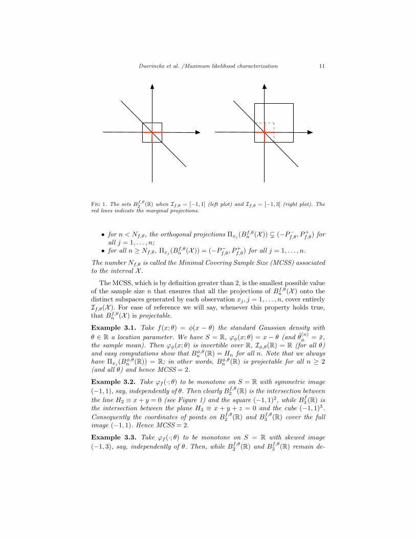
Fig 1. The sets Bf,θ2 (R) when If,θ = [−1, 1] (left plot) and If,θ = [−1, 3] (right plot). Thered lines indicate the marginal projections.

• for n < Nf,θ, the orthogonal projections Πxj (Bf,θn (X )) ( (−P−f,θ, P

+f,θ) for

all j = 1, . . . , n;• for all n ≥ Nf,θ, Πxj (B

f,θn (X )) = (−P−f,θ, P

+f,θ) for all j = 1, . . . , n.

The number Nf,θ is called the Minimal Covering Sample Size (MCSS) associatedto the interval X .

The MCSS, which is by definition greater than 2, is the smallest possible valueof the sample size n that ensures that all the projections of Bf,θn (X ) onto thedistinct subspaces generated by each observation xj , j = 1, . . . , n, cover entirelyIf,θ(X ). For ease of reference we will say, whenever this property holds true,that Bf,θn (X ) is projectable.

Example 3.1. Take f(x; θ) = φ(x − θ) the standard Gaussian density with

θ ∈ R a location parameter. We have S = R, ϕφ(x; θ) = x − θ (and θ(n)φ = x,

the sample mean). Then ϕφ(x; θ) is invertible over R, Iφ,θ(R) = R (for all θ)and easy computations show that Bφ,θn (R) = Hn for all n. Note that we alwayshave Πxj (B

φ,θn (R)) = R; in other words, Bφ,θn (R) is projectable for all n ≥ 2

(and all θ) and hence MCSS = 2.

Example 3.2. Take ϕf (·; θ) to be monotone on S = R with symmetric image

(−1, 1), say, independently of θ. Then clearly Bf,θ2 (R) is the intersection between

the line H2 ≡ x+ y = 0 (see Figure 1) and the square (−1, 1)2, while Bf3 (R) isthe intersection between the plane H3 ≡ x + y + z = 0 and the cube (−1, 1)3.

Consequently the coordinates of points on Bf,θ2 (R) and Bf,θ3 (R) cover the fullimage (−1, 1). Hence MCSS = 2.

Example 3.3. Take ϕf (·; θ) to be monotone on S = R with skewed image

(−1, 3), say, independently of θ. Then, while Bf,θ2 (R) and Bf,θ3 (R) remain de-


fined as in Example 3.2 (with (−1, 3) replacing (−1, 1)), coordinates of points in

these domains do not cover the full image. In fact, in Bf,θ2 (R) these coordinates

only cover the interval (−1, 1) (see Figure 1), in Bf,θ3 (R) these coordinates onlycover the interval (−1, 2) and it is only from n ≥ 4 onwards that the coordinatesof points in Bf,θn (R) cover the full image. Hence MCSS = 4.

Example 3.4. Take f(x; θ) = θφ(θx) the Gaussian density with θ ∈ R+0 a scale

parameter. We have S = R, ϕφ(x; θ) = 1θ (1− θ2x2). Then ϕφ(·; θ) is invertible

over R+0 and R−0 , separately, and If,θ(R±0 ) = (−∞, 1/θ). Note that we have

Πxj (Bf,θn (R±0 )) = (−(n − 1)/θ, 1/θ) for all j, all θ and all n ≥ 2. In other

words, Bf,θn (R±0 ) is only asymptotically projectable. Hence MCSS = +∞.

Proof of Lemma 3.1. The assumptions on the image of ϕf (·; θ) guarantee the

existence of a point in X where ϕf crosses the x-axis so that Bf,θ1 (X ) = {0}.Also, for all n ≥ 1, we have Bf,θn (X ) = Hn∩(If,θ(X ))n; this follows by definition.Regarding the MCSS, first take P−f,θ = P+

f,θ = P (possibly infinite). Then, forall n ≥ 2, Hn ∩ (−P, P )n contains for each of the n coordinates the full interval(−P, P ) (see Figure 1); hence MCSS = 2. Next suppose that P−f,θ < P+

f,θ <∞ and consider a “worst-case scenario” by taking a point at the extreme ofHn ∩ (If,θ(X ))n, with one coordinate set to b1 = P+

f,θ − ε for some ε > 0. Then,

in order to construct a sample satisfying∑ni=1 bi = 0, it is necessary to choose

the remaining n− 1-tuple (b2, . . . , bn) so as to satisfy∑ni=2 bi = −b1. Since the

best choice in this respect consists in setting all bi near the other extremum−P−f,θ + ε′ for ε′ > 0, we see that, depending on the magnitude of the ratio

P+f,θ/P

−f,θ, a given sample size n may not be large enough for the equality to

hold. In order to palliate this it suffices to take Nf,θ to be the smallest natural

number such that P+f,θ − (Nf,θ − 1)P−f,θ ≤ 0, that is Nf,θ =

⌈P+f,θ/P

−f,θ + 1

⌉.

The case P+f,θ < P−f,θ <∞ follows along the same lines, and hence

MCSS =

⌈max(P+

f,θ, P−f,θ)

min(P+f,θ, P

−f,θ)

+ 1

⌉.

The same argumentation applies in the case where either one of P+f,θ or P−f,θ is

infinite, this time with MCSS = +∞. This concludes the proof.

Now look at the connection between the MCSS and MLE characterizations.Let f and g be two representatives of distinct e.c.’s with f the target density.Under the assumption of θ-differentiability of g, the defining equation (4) canbe re-expressed as

n∑i=1

ϕg(xi; θ(n)f (x(n))) = 0 for all x(n) ∈ Sn,

which in turn can be rewritten asn∑i=1

ϕg(xi; θ) = 0 for all θ and all x(n) such that

n∑i=1

ϕf (xi; θ) = 0, (7)


(here θ and x(n) are interdependent) or, equivalently,

n∑i=1

h(yi; θ) = 0 for all θ and all y(n) ∈ Bf,θn (X ) (8)

for each interval X on which y 7→ ϕf (y; θ) is invertible for all θ, with h(y; θ) =ϕg(ϕ

−1f (y; θ); θ). Equation (8) completely identifies the function h (and hence

the interconnection between g and f), at least when Bf,θn (X ) is sufficiently rich.This richness depends strongly on the MCSS introduced in Lemma 3.1. Indeedsupposing that (8) is only valid for a sample size smaller than the MCSS impliesthat portions of the images If,θ(X ) cannot be reached, so that h cannot beidentified over its entire support. This necessarily implies that MNSS ≥ MCSS.It is, however, pointless to try to solve (8) in all generality and it is now necessaryto specify the role of θ in order to pursue. We will do so in detail in the nextsections, first in the case of location parameters; our arguments will afterwardsadapt directly to other parameter choices.

4. MLE characterization for location parameter families

We start by identifying the e.c.’s for θ a location parameter. In such a case,Θ0 = S = R, and the location score functions are of the form ϕf (x; θ) =ϕf (x − θ) = −f ′(x − θ)/f(x − θ) over R, so that equation (3) turns into asimple first-order differential equation whose solution yields g(x) = c(f(x))d forsome d > 0 and c the normalizing constant. Thus, all densities which are linkedone to another via that relationship belong to a same e.c. We here attract thereader’s attention to the fact that, for f = φ the standard Gaussian density, suchtransformations reduce to a non-specification of the variance, which is clearly inline with Gauss’ MLE characterization as stated by Teicher (1961) or Azzaliniand Genton (2007).

Our first main theorem is, in essence, a generalization of Gauss’ MLE char-acterization from the Gaussian distribution to the entire class of log-concavedistributions with continuous score function.

Theorem 4.1. Let F(loc) and G(loc) be two distinct location-based e.c.’s andlet their respective representatives f and g be two continuously differentiabledensities with full support R. Let x 7→ ϕf (x) = −f ′(x)/f(x) be the locationscore function of f . If ϕf is invertible over R and crosses the x-axis then there

exists N ∈ N such that, for any n ≥ N , we have θ(n)f = θ

(n)g for all samples of

size n if and only if there exist constants c, d ∈ R+0 such that g(x) = c(f(x))d

for all x ∈ R, that is, if and only if F(loc) = G(loc). The smallest integer forwhich this holds (the Minimal Necessary Sample Size) is MNSS = max{Nf , 3},with Nf the MCSS as defined in Lemma 3.1.

Proof. The sufficient condition is trivial. To prove necessity first note how ourassumptions on f ensure that the score function ϕf is strictly increasing onthe whole real line R and has a unique root. This allows us to write the image


Im(ϕf ) as (−P−f , P+f ) with 0 < P−f , P

+f ≤ ∞. The differentiability of g and the

nature of the parameter θ permit us to rewrite, for any admissible θ, (7) as

n∑i=1

ϕg(xi − θ) = 0 for all x(n) ∈ Rn such that

n∑i=1

ϕf (xi − θ) = 0, (9)

where ϕg(x) = −g′(x)/g(x). Using the strict monotonicity of ϕf one then con-cludes that (9) is equivalent to requiring that g satisfies

n∑i=1

h(bi) = 0 for all (b1, . . . , bn) ∈ Bf,θn (R) (10)

where h = ϕg ◦ϕ−1f and bi = ϕf (xi− θ), i = 1, . . . , n, as in (5). In what follows,

we shall use our liberty of choice among all n-tuples b(n) ∈ Bf,θn (R) in order togain sufficient information on h to conclude.

First suppose that P−f,θ = P+f,θ = P , hence that the image of ϕf is symmetric.

We know from Lemma 3.1 that the corresponding MCSS equals 2, hence thattwo observations suffice to make Bf,θn (R) projectable. Therefore, for any n ≥ 2,we can always build an n-tuple b1, . . . , bn such that b2 = −b1 for all b1 ∈ (−P, P )and bi = 0 for i = 3, . . . , n. From (10) we then deduce that h satisfies the equalityh(−a) = −h(a) for all a ∈ (−P, P ), hence that h is odd on (−P, P ). Evidentlythis leaves h undetermined, hence the MNSS must at least equal 3. For n ≥ 3,choose an n-tuple such that b3 = −b1 − b2 and bi = 0 for i = 4, . . . , n, forb1, b2 ∈ (−P, P ) such that b1 + b2 ∈ (−P, P ). Using (10) combined with theantisymmetry of h we deduce that this function must satisfy

h(b) + h(c) = h(b+ c) (11)

for all b, c ∈ (−P, P ) such that b + c ∈ (−P, P ). One recognizes in (11) a(restricted) form of the celebrated Cauchy functional equation. Assume thatP < ∞; then h(P/2), say, is finite and standard arguments (see, e.g., (Aczeland Dhombres, 1989)), imply that our solution h satisfies h(uP/2) = uh(P/2)for all u ∈ (−2, 2) and we conclude that h(x) = d x for all x ∈ (−P, P ), withd = h(P/2)/(P/2) ∈ R. Considering x = ϕf (y) for y ∈ ϕ−1f (−P, P ) = R, weobtain that ϕg(y) = dϕf (y). Solving this first-order differential equation givesg(y) = c(f(y))d for all y ∈ R, with c a constant. In order for the function g tobe integrable over R, the constant d must be strictly positive; in order for g tobe positive and integrate to 1, the constant c must be a normalizing constant.Thus, for P < ∞, the problem is solved. For P = ∞, the situation becomeseven simpler as (11) is then precisely the Cauchy functional equation, and onemay immediately draw the same conclusion as for finite P .

Let us now consider the case where ϕf has a skewed image and set P =min(P−f , P

+f ) (note that P is necessarily finite as otherwise Im(ϕf ) would be

symmetric). First restricting our attention to (−P, P ), we can repeat the abovearguments to deduce that g(y) = c(f(y))d for all y ∈ ϕ−1f (−P, P ) ( R. We thusfurther need to investigate the behavior of h on the remaining part of Im(ϕf )


which, for the sake of simplicity, we denote as Out(P ) (it is either (−P−f ,−P )

or (P, P+f )). To this end, we precisely need to know the MCSS and hence call

upon Lemma 3.1. Fixing n ≥ Nf and taking a sample (b1, . . . , bn) such that∑ni=1 bi = 0 with b1 ∈ Out(P ) and (b2, . . . , bn) ∈ (−P, P )n−1, we can apply

(10) to get h(b1) +∑ni=2 h(bi) = 0 and hence, from our knowledge about the

behavior of h on (−P, P ), we deduce that

h(b1) = −n∑i=2

bih(P )/P = b1h(P )/P,

since h(P ) is necessarily finite. Consequently we get h(y) = yh(P )/P for ally ∈ (−P, P ) ∪ Out(P ) = Im(ϕf ) and g(y) = c(f(y))d for all y ∈ R, and theconclusion follows.

The proof of the theorem is nearly complete : all that remains is to show thatthe MNSS = max{3, Nf} is minimal and sufficient. The latter is immediate sinceif the result holds true for any sample of size N = MNSS then, for any largersample size M > MNSS, one can always consider x(M) such that ϕf (x(M)) =

b(M) ∈ Bf,θM (R) is of the form (b1, . . . , bN , 0, . . . , 0) and (b1, . . . , bN ) ∈ Bf,θN (R),and work as above to characterize the density. To prove the minimality of theMNSS it suffices to exhibit specific counter-examples. This is done in Examples4.1 and 4.2 below.

Example 4.1. To see that N = 3 is minimal when Im(ϕf ) is symmetric, weneed to construct two distributions g1, g2 which share f ’s MLE for all samples ofsize 2. Construct g1 as in the proof of Theorem 4.1. To construct g2 it sufficesto replace the function h from (10) with any odd function and to solve theresulting equation in g (while ensuring integrability of g). If, for example, wechoose h(x) = dx3, then we readily obtain g(y) = c exp(−d

∫ x−∞(ϕf (y))3dy); this

is however not a density for all f , though a good choice for f = φ the Gaussian(for which ϕφ(x) = x). Another way of proceeding is to work as in Azzaliniand Genton (2007) and to choose h(y) = y+w′(y) for some differentiable evenfunction w.

Example 4.2. Suppose that θ(n)f = θ

(n)g for all samples of size n for some

n < Nf when Nf > 3. Then, as is clear from Lemma 3.1, the whole domain(that is, R) of f is not identified by our technique and it suffices to choose anydensity which is equal to f on the maximal identifiable subdomain but differselsewhere. Expressed in terms of h for the case P−f < P+

f , we can only identify

h on some interval (−P−f , P−f + a(n)), say, with 0 < a(n) < P+

f − P−f . On

the remaining part (P−f + a(n), P+f ), h is undetermined and hence can take

any possible form, implying that the relationship between g and f can only beestablished on the part ϕ−1f (−P−f , P

−f + a(n)) ( R.

As in Azzalini and Genton (2007), it is sufficient to require in Theorem 4.1that g be continuously differentiable at a single point for everything to runsmoothly. Pursuing in this vein, it is of course natural to enquire whether theresult still holds if no such regularity assumption is imposed on g, i.e. if we only


suppose that the target density f is differentiable but g is a priori not. Putsimply the question becomes that of enquiring whether the condition

n∑i=1

log g(xi − θ(n)f (x(n))) ≥n∑i=1

log g(xi − θ) (12)

for all x(n) ∈ Rn and all θ ∈ R suffices to determine g. This is the approachadopted, e.g., in Teicher (1961); Kagan, Linnik and Rao (1973) or Marshall andOlkin (1993), where it is shown that having the likelihood condition (12) with

θ(n)f the sample mean implies g is the Gaussian as soon as the result holds for

all samples of sizes 2 and 3 simultaneously. Interestingly, in our framework, thisarguably more general assumption on g comes with a cost : our method of proofthen necessitates imposing more restrictive assumptions on f and requiring thelikelihood equations to hold for two sample sizes simultaneously.

Theorem 4.2. Let F(loc) and G(loc) be two distinct location-based e.c.’s andlet their respective representatives f and g be two continuous densities with fullsupport R. Suppose that f is symmetric and continuously differentiable, andassume that its location score function ϕf (x) is invertible over R and crosses

the x-axis. Then we have θ(n)f = θ

(n)g for all samples of sizes 2 and n ≥ 3

simultaneously if and only if there exist constants c, d ∈ R+0 such that g(x) =

c(f(x))d for all x ∈ R, that is, if and only if F(loc) = G(loc).

Proof. Our proof, which extends that of Teicher (1961) from the Gaussian caseto the entire class of symmetric log-concave densities f , proceeds in two mainsteps: we first show that our assumptions on g in fact entail that g is continu-ously differentiable, and then conclude by applying Theorem 4.1. The additionalsample size n = 2 needed here stems from the first step.

Condition (12) can be rewritten as

n∑i=1

log g(yi) ≥n∑i=1

log g(yi − θ)

for all θ ∈ R and y1, . . . , yn satisfying∑ni=1 ϕf (yi) = 0. The latter expression in

turn is equivalent to

n−1∑i=1

log g(yi) + log g

ϕ−1f− n−1∑

j=1

ϕf (yj)

≥n−1∑i=1

log g(yi − θ) + log g

ϕ−1f− n−1∑

j=1

ϕf (yj)

− θ . (13)

Arguing as in Teicher (1961), it is sensible to confine our attention at first tosymmetric densities g. Using the assumed symmetric nature of f (and hence theoddness of ϕ−1f ), considering the sample size n = 2 and setting observation y1


equal to some y ∈ R, (13) simplifies into

2 log g(y) ≥ log g(y − θ) + log g(y + θ) (14)

for all y, θ ∈ R. Since log g is everywhere finite, concave according to (14), andinherits measurability from g, it is an a.e.-continuously differentiable function.Arrived at this point, we may apply Theorem 4.1 to conclude (note that theoddness of ϕf makes Theorem 4.1 hold with MNSS equal to 3).

Finally, for non-necessarily symmetric densities g, we can follow exactly theargumentation from Teicher (1961) and derive that the previously obtainedsolution is the only one, hence the claim holds.

We stress the fact that, as in Teicher (1961), we may further weaken ourassumptions on g by only requiring that it is lower semi-continuous at the originand need not have full support R. Indeed, as shown in Teicher’s proof, continuityand a.e.-positivity ensue from the above arguments.

One may wonder whether the symmetry assumption on the target density f isnecessary or whether this second general location MLE characterization theoremmay in fact hold for the entire class of log-concave densities as well. Our methodof proof indeed requires this assumption so as to enable us to deal with suchquantities as ϕ−1f (−

∑n−1j=1 ϕf (yj)) in (13); without any assumption on f , for

n = 2, this expression does not simplify into the agreeable form −y1. Similarlyone may wonder whether it is necessary to suppose the result to hold for twosample sizes simultaneously or whether one single sample size N ≥ 3 might notsuffice. We leave as open problems the question whether these assumptions arenecessary or simply sufficient.

Finally our Theorems 4.1 and 4.2 do not cover target densities whose locationscore function is monotone but not invertible over the entire real line, that is,piecewise constant. We do not consider explicitly such setups here since they donot assure that the MLE is defined in a unique way. The strategy we howeversuggest consists in applying our results on the monotonicity intervals, to drawthe necessary conclusions and express g in terms of f on those intervals. If weadd the condition of monotonicity of ϕg, the equality ϕg(x) = dϕf (x) has to holdover the entire support R as monotonicity imposes ϕg to be constant outsidethe above-mentioned intervals. Since we here do not implicitly use the intervalswhere ϕf is constant, there might exist better strategies, and consequently thesmallest possible sample size we obtain by following this scheme is an upperbound for the true MNSS. The most extreme situation takes place when thetarget is a Laplace distribution, in which case ϕf (x) = sign(x); we refer toKagan, Linnik and Rao (1973) for a treatment of this particular distribution.We will return to these matters briefly in Section 8.

5. MLE characterization for scale parameter families

As for location parameter families, we start by identifying the e.c.’s when θplays the role of a scale parameter. In such a setup, Θ0 = R+

0 , S = R, R+0 or


R−0 in view of Assumption (A2), and the scale score functions are of the formϕf (x; θ) = 1

θψf (θx) := 1θ (1+θxf ′(θx)/f(θx)) over S, so that equation (3) turns

into another quite simple first-order differential equation whose solution leadsto g(x) = c|x|d−1(f(x))d for some d > 0 (such that g is integrable) and c thenormalizing constant. This relationship defines the scale-based e.c.’s. It is to benoted that c = d = 1 when the origin belongs to the support, that is, whenS = R, in which case the e.c.’s reduce to singletons {f}.

Our main scale MLE characterization theorem is the exact equivalent ofTheorem 4.1 with ψf replacing ϕf , hence its proof is omitted.

Theorem 5.1. Let F(sca) and G(sca) be two distinct scale-based e.c.’s and lettheir respective representatives f and g be two continuously differentiable densi-ties with common support S (either R,R+

0 or R−0 ). Let ψf (x) = 1+xf ′(x)/f(x)be the scale score function of f . If ψf is invertible over S and crosses the x-

axis then there exists N ∈ N such that, for any n ≥ N , we have θ(n)f = θ

(n)g

for all samples of size n if and only if there exist constants c, d ∈ R+0 such

that g(x) = c|x|d−1(f(x))d for all x ∈ S (with c = d = 1 for S = R), thatis, if and only if F(sca) = G(sca). The smallest integer for which this holds isMNSS = max{Nf , 3}, with Nf the MCSS as defined in Lemma 3.1.

As in the case of a location parameter, requiring differentiability of the g’sis not indispensable. One could indeed restrict the class of target distributionsunder consideration, as in Teicher (1961). We leave this as an easy exercise.

When dealing with scale families it is natural to work as in Teicher (1961)and add a scale-identification condition of the form

limx→0

g(λx)/g(x) = limx→0

f(λx)/f(x) ∀λ > 0. (15)

Imposing this condition in Theorem 5.1 allows, at least when the limit is finite,positive and does not equal 1/λ (which occurs only for pathological cases; weleave as an exercise to the reader to see why this type of limiting behaviorprecludes identifications), to deduce that c = d = 1 for S = R+

0 and R−0 ,and hence g = f in all cases. Interestingly Teicher already remarks that this“seemingly ad hoc condition appears to be crucial”; this is clearly the case for acomplete identification of the family of densities which share a scale MLE.

The invertibility condition imposed on ψf is as natural in a scale family con-text as the invertibility condition on ϕf in a location family setup (see (Lehmannand Casella, 1998, page 502)). Unfortunately it suffers from one major draw-back for S = R: requiring invertibility of ψf over the whole real line forces usto discard several interesting cases such as, e.g., the standard normal density φ,for which ψφ(x) = 1 − x2 is only invertible over the positive and negative realhalf-lines, respectively. More generally any symmetric density f for which ϕfis invertible over R will suffer from that same problem and hence will not becharacterizable by means of Theorem 5.1. This flaw is nevertheless easily fixed,since Lemma 3.1 is applicable even if ψf is only invertible over portions of itssupport. This leads to our next general result (whose proof is omitted).


Theorem 5.2. Let F(sca) and G(sca) be two distinct scale-based e.c.’s and lettheir respective representatives f and g be two continuously differentiable densi-ties with full support R. Let the scale score function ψf (x) = 1 +xf ′(x)/f(x) beinvertible and cross the x-axis over R+

0 and R−0 , respectively. Then there exists

N ∈ N such that, for any n ≥ N , we have θ(n)f = θ

(n)g for all samples of size

n if and only if g(x) = f(x) for all x ∈ R. Moreover the MNSS is given bymax{MNSS−,MNSS+}, where MNSS− and MNSS+ respectively stand for theMNSS required on each half-line.

It should be noted that the scale condition (15) is not necessary here since weare working on the entire support S = R which imposes that d = 1 as otherwisethe non-vanishing density g would vanish at 0.

Finally note that the separation of the two real half-lines is tailored for scalefamilies because both R+

0 and R−0 are invariant under the action of the scaleparameter, which permits us to work on each half-line separately and put theends together by continuity. The same would not hold true for location fami-lies due to a lack of invariance, that is we could not “glue together” locationcharacterizations valid on complementary subsets of the support.

6. MLE characterization for one-parameter group families

The relevance of our approach is not confined to location and scale families, butcan be used for other θ-parameter families with θ neither a location nor a scaleparameter. In this section, we shall consider general one-parameter group fami-lies and provide them with MLE characterization results. Group families play acentral role in statistics as they contain several well-known parametric families(location, scale, several types of skew distributions as shown in Ley and Pain-daveine (2010a), . . . ) and allow for significant simplifications of the data underinvestigation (see (Lehmann and Casella, 1998, Section 1.4) for more details).To the best of the authors’ knowledge, there exist no MLE characterizations forgroup families other than the location and scale families.

A univariate group family of distributions is obtained by subjecting a scalarrandom variable with a fixed distribution to a suitable family of transformations.More prosaically, let X be a random variable with density f defined on itssupport S and consider a transformation group H (meaning that it is closedunder both composition and inversion) of monotone increasing functions Hθ :D ⊆ R→ S depending on a single real parameter θ ∈ Θ0. The family of randomvariables

{H−1θ (X), Hθ ∈ H

}is called a group family. These variables possess

densities of the formfH(x; θ) := H ′θ(x)f(Hθ(x)), (16)

where H ′θ stands for the derivative of the mapping x 7→ Hθ(x) (which we there-fore also suppose everywhere differentiable); their support D does not dependon θ. We call θ a H-parameter for f(x; θ). The most prominent examples areof course Hloc := {Hθ(x) = x − θ, x, θ ∈ R}, leading to location families, andHsca := {Hθ(x) = θx, x ∈ S, θ ∈ R+

0 } for S = R,R+0 and R−0 , yielding scale


families. For further examples, we refer to (Lehmann and Casella, 1998, Section1.4) and the references therein.

Let us now determine the e.c.’s for H-parameter families. Assuming that themappings θ 7→ Hθ(x) and θ 7→ H ′θ(x) are differentiable, the H-score functionassociated with densities of the form (16) corresponds to

ϕHf (x; θ) :=∂θH

′θ(x)

H ′θ(x)+∂θHθ(x)f ′(Hθ(x))

f(Hθ(x))(17)

over D (it is set to 0 outside D). Extracting e.c.’s from equation (3) is all butevident here, as (i) there is no structural reason for ∂θHθ(x) to cross the x-axisso as to allow to fix d to 1 as in the scale case over R, and (ii) the generality ofthe model hampers a clear understanding of the role of θ inside the densities.Especially the latter point is crucial, as e.c.’s cannot depend on the parameter.We thus need to further specify the form of fH(x; θ) or, more exactly, the formof the transformations in H and thus the action of θ inside the densities. Wechoose to restrict our attention to transformations Hθ satisfying the followingtwo factorizations: {

∂θHθ(x) = T (θ)U1(Hθ(x))∂θH

′θ(x)

H′θ(x)= T (θ)U2(Hθ(x)),

where T , U1 and U2 are real-valued functions. At first sight, such restrictionsmight seem severe, but there exist numerous one-parameter transformationsenjoying these factorizations, including

- transformations of the form Hθ(x) = a1(x) + a2(θ) defined over the entirereal line, with a1 a monotone increasing differentiable function over R anda2 any real-valued differentiable function. These transformations lead to“generalized location families” and satisfy the above factorizations withT (θ) = a′2(θ), U1(x) = 1 and U2(x) = 0.

- transformations of the form Hθ(x) = a1(x)a2(θ) defined over R,R+0 or

R−0 , with a1 a monotone increasing differentiable function over the cor-responding domain and a2 a positive real-valued differentiable function.These transformations lead to “generalized scale families” and satisfy theabove factorizations with T (θ) = a′2(θ)/a2(θ), U1(x) = x and U2(x) = 1.

- transformations of the form Hθ(x) = sinh(arcsinh(x) + θ) defined over R.These are the so-called sinh-arcsinh transformations put to use in Jonesand Pewsey (2009) in order to define sinh-arcsinh distributions which al-low to cope for both skewness and kurtosis. The above factorizations areverified for T (θ) = 1, U1(x) =

√1 + x2 and U2(x) = x/

√1 + x2.

Under these premisses, equation (3) becomes

d

(U2(Hθ(x)) + U1(Hθ(x))

f ′(Hθ(x))

f(Hθ(x))

)= U2(Hθ(x)) + U1(Hθ(x))

g′(Hθ(x))

g(Hθ(x))∀x ∈ D,


which can be rewritten as

d

(U2(x) + U1(x)

f ′(x)

f(x)

)= U2(x) + U1(x)

g′(x)

g(x)∀x ∈ S.

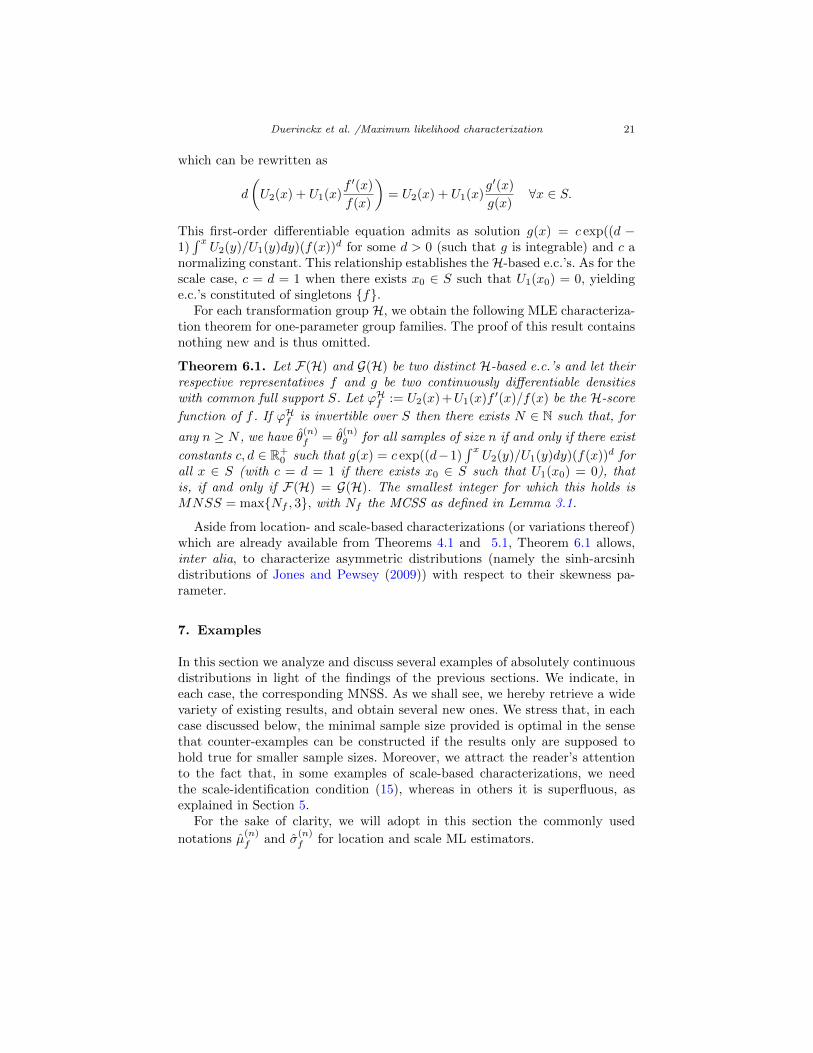
This first-order differentiable equation admits as solution g(x) = c exp((d −1)∫ x

U2(y)/U1(y)dy)(f(x))d for some d > 0 (such that g is integrable) and c anormalizing constant. This relationship establishes the H-based e.c.’s. As for thescale case, c = d = 1 when there exists x0 ∈ S such that U1(x0) = 0, yieldinge.c.’s constituted of singletons {f}.

For each transformation group H, we obtain the following MLE characteriza-tion theorem for one-parameter group families. The proof of this result containsnothing new and is thus omitted.

Theorem 6.1. Let F(H) and G(H) be two distinct H-based e.c.’s and let theirrespective representatives f and g be two continuously differentiable densitieswith common full support S. Let ϕHf := U2(x) +U1(x)f ′(x)/f(x) be the H-score

function of f . If ϕHf is invertible over S then there exists N ∈ N such that, for

any n ≥ N , we have θ(n)f = θ

(n)g for all samples of size n if and only if there exist

constants c, d ∈ R+0 such that g(x) = c exp((d−1)

∫ xU2(y)/U1(y)dy)(f(x))d for

all x ∈ S (with c = d = 1 if there exists x0 ∈ S such that U1(x0) = 0), thatis, if and only if F(H) = G(H). The smallest integer for which this holds isMNSS = max{Nf , 3}, with Nf the MCSS as defined in Lemma 3.1.

Aside from location- and scale-based characterizations (or variations thereof)which are already available from Theorems 4.1 and 5.1, Theorem 6.1 allows,inter alia, to characterize asymmetric distributions (namely the sinh-arcsinhdistributions of Jones and Pewsey (2009)) with respect to their skewness pa-rameter.

7. Examples

In this section we analyze and discuss several examples of absolutely continuousdistributions in light of the findings of the previous sections. We indicate, ineach case, the corresponding MNSS. As we shall see, we hereby retrieve a widevariety of existing results, and obtain several new ones. We stress that, in eachcase discussed below, the minimal sample size provided is optimal in the sensethat counter-examples can be constructed if the results only are supposed tohold true for smaller sample sizes. Moreover, we attract the reader’s attentionto the fact that, in some examples of scale-based characterizations, we needthe scale-identification condition (15), whereas in others it is superfluous, asexplained in Section 5.

For the sake of clarity, we will adopt in this section the commonly used

notations µ(n)f and σ

(n)f for location and scale ML estimators.


7.1. The Gaussian distribution

Consider the Gaussian distribution whose MLE characterizations for both thelocation and the scale parameter have been extensively discussed in the litera-ture. For φ the standard Gaussian density we get ϕφ(x) = x which is invertibleover R and has image Im(ϕφ) = R. As already mentioned several times, the MLE

µ(n)φ is given by the sample arithmetic mean x. Thus Theorems 4.1 and 4.2 apply,

with MNSS = 3 since P+φ = P−φ = ∞. The first corresponds to (Azzalini and

Genton, 2007, Theorem 1), the second to (Teicher, 1961, Theorem 1). Regarding

the scale characterization for σ(n)φ = (n−1

∑ni=1 x

2i )

1/2, direct calculations reveal

that ψφ(x) = 1 − x2 which is invertible over both R+0 and R−0 and maps both

domains onto (−∞, 1). The conditions of Theorem 5.2 are thus fulfilled andyield that the MNSS equals ∞. Hence we retrieve (Teicher, 1961, Theorem 3).

7.2. The gamma distribution

Consider the gamma distribution with tail parameter α > 0, whose density isgiven by

f(x) =1

Γ(α)xα−1 exp(−x)I(0,∞)(x),

where IA represents the indicator function of the set A. The exponential den-sity is a special case of gamma densities obtained by setting α = 1. Gammadistributions are not natural location families; this can be seen for instance byconsidering the exponential case, where ϕf (x) = 1 and hence the location like-lihood equations make no sense. Within the framework of the current paperwe anyway do not provide a location-based MLE characterization of gammadensities, since their support is only R+

0 instead of R. On the contrary, gammadensities allow for agreeable scale characterizations. Indeed easy computationsshow that ϕf (x) = (−α+ 1)/x+ 1, ψf (x) = α−x, which is thus invertible over

R+0 , Im(ψf ) = (−∞, α) and σ

(n)f = α−1x. We can therefore use Theorem 5.1

in combination with the scale-identification condition (15) to obtain that thegamma distribution with shape α is characterizable w.r.t. its scale MLE α−1xfor an infinite MNSS. We hereby recover (Teicher, 1961, Theorem 2) and theunivariate case of (Marshall and Olkin, 1993, Theorem 5.1).

7.3. The generalized Gaussian distribution

Consider the one-parameter generalization of the normal distribution proposedin Ferguson (1962), with density

f(x) =|γ|αα

Γ(α)exp(αγx− α exp(γx))

where α > 0 and γ, the additional parameter, differs from zero (Fergusonhas proved that, for γ → 0, this density converges to the Gaussian). This


probability law is in fact strongly related to the gamma distribution, as it isdefined as γ−1 log(X) with X ∼ Gamma(α). Now, direct calculations yieldϕf (x) = −αγ(1− exp(γx)), invertible over R, Im(ϕf ) = sign(γ)(−α|γ|,∞) and

µ(n)f = γ−1 log(n−1

∑ni=1 exp(γxi)). Hence, from Theorem 4.1, we deduce that

these distributions can be characterized in terms of their location parameter,with MNSS equal to ∞; we retrieve (Ferguson, 1962, Theorem 5). Concerningthe scale part, ψf (x) = αγx(1 − exp(γx)) + 1 is not invertible over the wholereal line, but invertible over both R+

0 and R−0 , and maps both half-lines onto(−∞, 1). Consequently, Theorem 5.2 reveals that this distribution admits aswell a scale MLE characterization result, with infinite MNSS.

7.4. The Laplace distribution

Consider the Laplace distribution with density

f(x) = exp(−|x|)/2.

One easily obtains ϕf (x) = sign(x) and ψf (x) = −xsign(x) + 1. While theformer function is clearly not invertible at all (but allows for a location MLEcharacterization; see the end of Section 5), the latter is invertible on both R−0and R+

0 with Im(ψf ) = (−∞, 1). Hence Theorem 5.2 applies and reveals thatthe Laplace distribution is also MLE-characterizable w.r.t. its scale parameter(with infinite MNSS), which complements the existing results on MLE char-acterizations of the Laplace distribution from Ghosh and Rao (1971); Kagan,Linnik and Rao (1973); Marshall and Olkin (1993).

Corollary 7.1. The statistic

σ(n)f =

(n−1

n∑i=1

|xi|

)−1is the MLE of the scale parameter σ within scale families over R for all sam-ples of all sample sizes if and only if the samples are drawn from a Laplacedistribution.

For the sake of readability we will, here and in the sequel, content ourselveswith such informal statements of our characterization results; rigorous state-ments are straightforward adaptations of the corresponding theorems from theprevious sections.

7.5. The Weibull distribution

Consider the Weibull distribution with density

f(x) = kxk−1 exp(−xk)I(0,∞)(x),


where k > 0 is the shape parameter. As for gamma distributions, we do notprovide a location-based MLE characterization for this distribution on the pos-itive real half-line. Regarding the scale part, we have ϕf (x) = −k−1x + kxk−1,

ψf (x) = k(1 − xk), clearly invertible over R+0 , and Im(ψf ) = (−∞, k). Thus,

all conditions for Theorem 5.1 are satisfied, from which we derive, under thescale-identification condition (15), the following, to the best of our knowledgenew, MLE characterization of the Weibull distribution.

Corollary 7.2. Let condition (15) hold. Then the statistic

σ(n)f =

(n−1

n∑i=1

xki

)−1/k

is the MLE of the scale parameter σ within scale families over R+0 for all sam-

ples of all sample sizes if and only if the samples are drawn from a Weibulldistribution with shape parameter k.

7.6. The Gumbel distribution

Consider the Gumbel distribution with density

f(x) = exp(−x− exp(−x)).

Straightforward manipulations yield ϕf (x) = 1 − exp(−x), invertible over Rand Im(ϕf ) = (−∞, 1). Thus, all conditions for Theorem 4.1 are satisfied, fromwhich we derive the following, to the best of our knowledge new, MLE character-ization of the Gumbel distribution (actually, of the power-Gumbel distribution).

Corollary 7.3. The statistic

µ(n)f = log

(n−1 n∑i=1

exp(−xi)

)−1is the MLE of the location parameter µ within location families over R for allsamples of all sample sizes if and only if the samples are drawn from a power-Gumbel distribution with density c exp(−dx− d exp(−x)) for c, d ∈ R+

0 .

As for the scale part, it follows that ψf (x) = x(−1 + exp(−x)) + 1, non-invertible over R but invertible over both R+

0 and R−0 , and Im(ψf ) = (−∞, 1).Consequently, Theorem 5.2 applies and shows that the Gumbel distribution(here not a general power-Gumbel distribution) allows as well for a MLE char-acterization with respect to its scale parameter (with corresponding MNSS equalto ∞).


7.7. The Student distribution

Consider the Student distribution with ν > 0 degrees of freedom, with density

f(x) = κ(ν)

(1 +

x2

ν

)−(ν+1)/2

,

for κ(ν) the appropriate normalizing constant. Then although the support of fis the whole real line, the location score function ϕf (x) = (ν + 1) x

ν+x2 is notinvertible and thus we cannot provide a location characterization. On the otherhand straightforward computations yield

ψf (x) = 1− (ν + 1)x2

ν + x2= −ν +

ν(ν + 1)

ν + x2.

This function is invertible over both the positive and the negative real half-line with Im(ψf ) = (−ν, 1) and thus the Student distribution with ν degrees offreedom is by virtue of Theorem 5.2 scale-characterizable with

MNSS =

d1 + 1ν e if ν < 1,

3 if ν = 1,d1 + νe if ν > 1.

This result generalizes the scale characterization of the Gaussian distribution,which is a particular case of the Student distributions when ν tends to infinity.Note that the expression above then indeed yields an infinite MNSS. Moreover,the Cauchy distribution, obtained for ν = 1, is MLE-characterizable w.r.t. itsscale parameter with an MNSS of 3.

7.8. The logistic distribution

Consider the logistic distribution, whose density is given by

f(x) =e−x

(1 + e−x)2.

Straightforward manipulations yield ϕf (x) = tanh(x/2), which is invertible overR and Im(ϕf ) = (−1, 1). Theorem 4.1 applies and yields the (to the best of ourknowledge) first MLE characterization of the (power-)logistic distribution withrespect to its location parameter (with corresponding MNSS equal to 3).

Further, ψf (x) = 1 − x tanh(x/2) is not invertible over the whole real line,but is invertible over both R+

0 and R−0 , and maps both half-lines onto (−∞, 1).Consequently, Theorem 5.2 applies and yields the (to the best of our knowledge)first scale MLE characterization of the logistic distribution, with infinite MNSS.


7.9. The sinh-arcsinh skew-normal distribution

As a final example, we consider the sinh-arcsinh skew-normal distribution ofJones and Pewsey (2009) whose density is given by

f(x) =1√2π

(1 + sinh2(arcsinh(x) + δ))1/2

(1 + x2)1/2e−sinh

2(arcsinh(x)+δ)/2,

where δ ∈ R is a skewness parameter regulating the asymmetric nature of thedistribution. Clearly, for δ = 0, corresponding to the symmetric situation, oneretrieves the standard normal distribution. Now, straightforward but tediouscalculations provide us with expressions for ϕf and ψf which can both be seento be non-invertible. Hence no location-based nor scale-based characterizationscan be obtained. However, the sinh-arcsinh skew-normal distribution can becharacterized w.r.t. its skewness parameter. As shown in Section 6, the sinh-arcsinh transform belongs to the class of transforms leading to group families.Consequently, its skewness score function is given by

ϕHf (x) = U2(x) + U1(x)φ′(x)

φ(x)=

−x3

(1 + x2)1/2,

with φ the standard Gaussian density. This mapping is invertible over R withsymmetric image R. Theorem 6.1 therefore applies and yields the (to the bestof our knowledge) first MLE characterization of the sinh-arcsinh skew-normaldistribution (with respect to its skewness parameter) with an MNSS equal to 3.

8. Discussion and open problems

In this article we have provided a unified treatment of the topic of MLE char-acterizations for one-parameter group families of absolutely continuous distri-butions satisfying certain regularity conditions. A natural question of interest isthen in how far our methodology can be adapted to other distributions which donot satisfy these assumptions. Of particular interest are (i) parametric familieswhose score function is either not invertible or not differentiable at a countablenumber of points (such as, e.g., the Laplace distribution w.r.t its location pa-rameter), (ii) families depending on more than one parameter and (iii) discretefamilies. Although we will not cover these questions in full here, we concludethe paper by providing a number of intuitions on these questions; in all casesit seems clear that our methodology provides – at least in principle – the pathtowards a satisfactory answer.

Regarding the first point, an interesting issue to investigate is how the non-invertibility of the score function influences the MNSS. Indeed in the case ofa Laplace target the MNSS is known to be equal to 4 (see (Ghosh and Rao,1971; Kagan, Linnik and Rao, 1973)). This increase is due to the fact that theLaplace score function only takes on two distinct non-zero values so that having(9) for three sample points forces one of the observations to be 0 (otherwise the


equality cannot hold) and therefore the case n = 3 provides no more informationthan the case n = 2 (and thus MNSS ≥ 4). It would of course be interesting tounderstand the influence of the number of distinct values taken by a given scorefunction on the corresponding MNSS. One would, moreover, need to deal in thiscase with commensurability issues in order for the corresponding identity (9)to hold; this would most certainly lead to interesting discussions. Aside fromthese issues, however, the question of characterizability is, to the best of ourunderstanding, covered by our approach (see the end of Section 4).

Regarding the second point, it seems straightforward (but clearly requiressome care) to extend our method to a multi-dimensional location parameter, asis already done in Marshall and Olkin (1993) for a Gaussian target density. In anutshell it suffices to project the now multi-dimensional location score functiononto distinct-directional unit vectors and then proceed “as in the univariatecase”. On the contrary, dealing with a high-dimensional scale parameter seemsmore difficult, as the scale parameter becomes a matrix-valued scatter or shapeparameter. One possibility could be to try to adapt Marshall and Olkin (1993)’sworking scheme, who have been able to provide an MLE characterization for thescatter parameter of a multinormal distribution. Along these lines a final issuethat we have not considered is that of MLE characterizations of univariate targetdistributions with respect to multivariate parameters (such as the Gaussianin terms of its two parameters (µ, σ)). In support of our optimism for thesemultivariate setups, see Duerinckx and Ley (2012) where our methodology wassuccessfully applied to the (perhaps more complex) case of the spherical locationparameter families.

Finally concerning the discrete setup it seems clear that our approach againyields in principle a satisfactory answer for discrete group families, althoughthis will require a certain amount of work. We defer the systematic treatmentof this interesting question to later publications.

We conclude this paper by an intriguing question suggested by an anonymousreferee, which is the following: do characterization results survive mixtures ofdistributions? More concretely, if a given distribution is MLE-characterizablew.r.t. a given parameter of interest, under which conditions will mixtures ofthis distribution remain MLE-characterizable? This question is all but straight-forward to answer. Indeed, we have seen in Section 7 that the Student distri-bution is only characterizable w.r.t. its scale parameter, whereas the logisticdistribution admits an MLE characterization w.r.t. both the location and scaleparameter; the Student and the logistic distribution are both scale mixtures ofthe Gaussian distribution, which is MLE-characterizable both as a location andscale family. We leave this question as an open problem.

Acknowledgements

All three authors thank Johan Segers and Davy Paindaveine for their interestingcomments during presentations of preliminary versions of this paper. The au-thors are also very grateful to two anonymous referees for extremely interesting


remarks and suggestions that have led to a definite improvement of the presentpaper.

References

Aczel, J. and Dhombres, J. (1989). Functional Equations in Several Variableswith Applications to Mathematics, Information Theory and to the Naturaland Social Sciences. In Encyclopedia Math. Appl., 31 Cambridge: CambridgeUniversity Press.

Akaike, H. (1977). On entropy maximization principle. In Applications ofStatistics (P. R. Krishnaiah, ed.).

Akaike, H. (1978). A Bayesian analysis of the minimum A.I.C. procedure. Ann.Math. Statist. 30 9–14.

Azzalini, A. and Genton, M. G. (2007). On Gauss’s characterization of thenormal distribution. Bernoulli 13 169–174.

Bondesson, L. (1997). A generalization of Poincare’s characterization of ex-ponential families. J. Statist. Plann. Inference 63 147–155.

Bourguin, S. and Tudor, C. A. (2011). Cramer theorem for gamma randomvariables. Electron. Commun. Probab. 16 365–378.

Buczolich, Z. and Szekely, G. J. (1989). When is a weighted average ofordered sample elements a maximum likelihood estimator of the location pa-rameter? Adv. in Appl. Math. 10 439–456.

Campbell, L. L. (1970). Equivalence of Gauss’s Principle and Minimum Dis-crimination Information Estimation of Probabilities. Ann. Math. Statist. 411011–1015.

Chatterjee, S. K. (2003). Statistical thought: a perspective and history. Ox-ford University Press, Oxford.

Chen, L. H. Y. (1975). Poisson approximation for dependent trials. Ann.Probab. 3 534–545.

Chen, L. H. Y., Goldstein, L. and Shao, Q. M. (2010). Normal Approxi-mation by Stein’s Method. Springer Series in Probability and its Applications.Springer-Verlag.

Cover, T. M. and Thomas, J. A. (2006). Elements of information theory.Wiley-interscience.

Cramer, H. (1936). Uber eine Eigenschaft der normalen Verteilungsfunktion.Math. Z. 41 405–414.

Cramer, H. (1946a). A contribution to the theory of statistical estimation.Skand. Aktuarietidskr. 29 85–94.

Cramer, H. (1946b). Mathematical Methods of Statistics. Princeton Mathe-matical Series, vol. 9. Princeton University Press, Princeton, N. J.

Duerinckx, M. and Ley, C. (2012). Maximum likelihood characterizationof rotationally symmetric distributions on the sphere. Sankhya Ser. A, toappear.

Ferguson, T. S. (1962). Location and scale parameters in exponential familiesof distributions. Ann. Math. Statist. 33 986–1001.


Findeisen, P. (1982). Die Charakterisierung der Normalverteilung nach Gauß.Metrika 29 55–63.

Galambos, J. (1972). Characterization of certain populations by independenceof order statistics. J. Appl. Probab. 9 224-230.

Gauss, C. F. (1809). Theoria motus corporum coelestium in sectionibus coni-cis solem ambientium. Cambridge Library Collection. Cambridge UniversityPress, Cambridge. Reprint of the 1809 original.

Ghosh, J. K. and Rao, C. R. (1971). A note on some translation parameterfamilies of densities for which the median is an m.l.e. Sankhya Ser. A 3391–93.

Haikady, N. N. (2006). Characterizations of Probability Distributions, part aed. Springer Handbook of Engineering Statistics 79-95. Springer-Verlag, Lon-don, UK.

Hald, A. (1998). A history of mathematical statistics from 1750 to 1930. WileySeries in Probability and Statistics: Texts and References Section. John Wiley& Sons Inc., New York.

Hurlimann, W. (1998). On the characterization of maximum likelihood esti-mators for location-scale families. Comm. Statist. Theory Methods 27 495–508.

Jaynes, E. T. (1957). Information theory and statistical mechanics. Physicalreview 106 620.

Jones, M. C. and Pewsey, A. (2009). Sinh-arcsinh distributions. Biometrika96 761-780.

Kagan, A. M., Linnik, Y. V. and Rao, C. R. (1973). Characterizationproblems in mathematical statistics. John Wiley & Sons, New York-London-Sydney.

Kendall, M. G., Bernoulli, D., G., A. C. and Euler, L. (1961). Studies inthe History of Probability and Statistics: XI. Daniel Bernoulli on MaximumLikelihood. Biometrika 48 1-18.

Kotz, S. (1974). Characterizations of Statistical Distributions: A Supplementto Recent Surveys. International Statistical Review / Revue Internationale deStatistique 42 39-65.

Lehmann, E. L. and Casella, G. (1998). Theory of point estimation, seconded. Springer Texts in Statistics. Springer-Verlag, New York.

Ley, C. and Paindaveine, D. (2010a). Multivariate skewing mechanisms: aunified perspective based on the transformation approach. Statist. Probab.Lett. 80 1685-1694.

Ley, C. and Paindaveine, D. (2010b). On the singularity of multivariate skew-symmetric models. J. Multivariate Anal. 101 1434-1444.

Lukacs, E. (1956). Characterization of populations by properties of suitablestatistics. In Proceedings of the Third Berkeley Symposium on “MathematicalStatistics and Probability” 195-214. University of California Press, Berkeley.

Marshall, A. W. and Olkin, I. (1993). Maximum likelihood characteriza-tions of distributions. Statist. Sinica 3 157–171.

Norden, R. H. (1972). A Survey of Maximum Likelihood Estimation. Int.Statist. Rev. 40 329–254.


Park, S. Y. and Bera, A. K. (2009). Maximum entropy autoregressive con-ditional heteroskedasticity model. J. Econometrics 150 219-230.

Patil, G. P. and Seshadri, V. (1964). Characterization Theorems for SomeUnivariate Probability Distributions. J. R. Stat. Soc. Ser. B Stat. Methodol.26 286-292.

Poincare, H. (1912). Calcul des probabilites. Carre-Naud, Paris.Puig, P. (2003). Characterizing additively closed discrete models by a property

of their MLEs, with an application to generalized Hermite distributions. J.Amer. Statist. Assoc. 98 687-692.

Puig, P. (2008). A note on the harmonic law : a two-parameter family ofdistributions for ratios. Statist. Probab. Lett. 78 320–326.

Puig, P. and Valero, J. (2006). Count data distributions: some characteriza-tions with applications. J. Amer. Statist. Assoc. 101 332-340.

Ross, N. (2012). Fundamentals of Stein’s method. Probab. Surveys.Stein, C. (1972). A bound for the error in the normal approximation to the

distribution of a sum of dependent random variables. Proc. Sixth BerkeleySymp. Math. Statist. Probab. 2 583-602.

Stigler, S. (1999). Statistics on the table: The history of Statistical Conceptsand Methods. Harvard University Press, Cambridge, Massachusetts, London,England.

Stigler, S. (2007). The epic story of Maximum Likelihood. Statistical Science22 598–620.

Teicher, H. (1961). Maximum likelihood characterization of distributions.Ann. Math. Statist. 32 1214–1222.

von Mises, R. (1918). Physikalische Zeitschrift 19 490-500.Wu, X. (2003). Calculation of maximum entropy densities with application to

income distribution. Journal of Econometrics 115 347–354.

Maximum likelihood characterization of distributions - ULiege Bernoulli... · Abstract: A famous...

Documents

Transcript of Maximum likelihood characterization of distributions - ULiege Bernoulli... · Abstract: A famous...