
A Lifetime-Optimizing Approach to Routing Messages in Ad ...
Southern Illinois University CarbondaleOpenSIUC
Theses Theses and Dissertations
8-1-2011
Maximizing the System Lifetime in Wireless SensorNetworks using Improved Routing AlgorithmKarthik KuppaswamySouthern Illinois University Carbondale, [email protected]
Follow this and additional works at: http://opensiuc.lib.siu.edu/theses
This Open Access Thesis is brought to you for free and open access by the Theses and Dissertations at OpenSIUC. It has been accepted for inclusion inTheses by an authorized administrator of OpenSIUC. For more information, please contact [email protected].
Recommended CitationKuppaswamy, Karthik, "Maximizing the System Lifetime in Wireless Sensor Networks using Improved Routing Algorithm" (2011).Theses. Paper 677.
MAXIMIZING THE SYSTEM LIFETIME IN WIRELESS SENSOR NETWORKS
USING IMPROVED ROUTING ALGORITHM
by
Karthik Kuppaswamy
B.E., Visvesvaraya Technological University, 2007
A Thesis Submitted in Partial Fulfillment of the Requirements for the
Master of Science Degree
Department of Electrical and Computer Engineering
in the Graduate School Southern Illinois University Carbondale
August 2011

THESIS APPROVAL
MAXIMIZING THE SYSTEM LIFETIME IN WIRELESS SENSOR NETWORKS
USING IMPROVED ROUTING ALGORITHM
By
Karthik Kuppaswamy
A Thesis Submitted in Partial
Fulfillment of the Requirements
for the Degree of
Master of Science
in the field of Electrical and Computer Engineering
Approved by:
Dr. Dimitrios Kagaris, Chair
Dr. Ning Weng
Dr. Ada Chen
Graduate School Southern Illinois University Carbondale
April 28th, 2011.

i
AN ABSTRACT OF THE THESIS OF
KARTHIK KUPPASWAMY, for the Master of Science degree in Electrical and Computer Engineering, presented on April 28th 2011, at Southern Illinois University Carbondale. TITLE: MAXIMIZING THE SYSTEM LIFETIME IN WIRELESS SENSOR
NETWORKS USING IMPROVED ROUTING ALGORITHM
MAJOR PROFESSOR: Dr. Dimitrios Kagaris In wireless sensor networks, the maximum lifetime routing problem has received
increasing attention among researchers. There are several critical features that
need to be considered while designing a wireless sensor networks such as cost,
network lifetime and Quality of service. Due to the limitation on the energy of
sensor nodes, energy efficient routing is a very important issue in sensor
networks. Therefore, to prolong the lifetime of the sensor nodes, designing
efficient routing protocols is critical. One solution is to formulate the routing
problem as a linear programming problem by maximizing the time at which the
first node runs out of battery. In this paper, with the notion of maximizing the
system lifetime, we implemented a new heuristic and evaluated the performance
of it with the existing algorithm called flow augmentation algorithm. Further, our
experimental results demonstrate that the proposed algorithm significantly
outperform FA algorithm, in terms of system lifetime.

ii
ACKNOWLEDGMENTS
I want to thank Lord Balaji, Goddess Karumari and my family for their teachings
and encouragement. I would like to thank my advisor, Dr. Dimitrios Kagaris , for
his invaluable assistance and insights, which helped me to successfully complete
this research paper. I am grateful to him for his patience with me throughout the
time and all the lessons he taught me for my career and life. I would also take
this opportunity to thank Sasi, Deepak, Dinesh and to all my friends who prayed
for me.

iii
TABLE OF CONTENTS
CHAPTER PAGE
ABSTRACT ....................................................................................................... i
ACKNOWLEDGMENTS ................................................................................... ii
LIST OF TABLES ............................................................................................ iv
LIST OF FIGURES .......................................................................................... vi
CHAPTERS
CHAPTER 1 – Introduction .................................................................... 1
CHAPTER 2 – Routing protocols for Sensor Networks ....................... 16
CHAPTER 3 – Methodology ................................................................ 34
CHAPTER 4 – Results and Conclusion ............................................... 63
REFERENCES ............................................................................................... 77
VITA ............................................................................................................. 80
iv
LIST OF TABLES
TABLE PAGE
Table 3.1 Meanings of the parameters in Algorithm FA .................................. 38
Table 3.2 Information generated for every origin node ................................... 43
Table 3.3 Reference table for residual energy update .................................... 44
Table 3.4 Residual energy update after first iteration ..................................... 45
Table 3.5 Residual energy update after second iteration ............................... 46
Table 3.6 Residual energy update after first iteration (Our Algorithm) ............ 48
Table 3.7 Residual energy update after second iteration (Our Algorithm) . 48-49
Table 3.8 Residual energy update after third iteration (Our Algorithm) ........... 49
Table 3.9 Residual energy update after fourth iteration (Our Algorithm) ........ 50
Table 3.10 Residual energy update after fifth iteration (Our Algorithm) .......... 51
Table 3.11 Residual energy update after sixth iteration (Our Algorithm) ... 51-52
Table 3.12 Residual energy update after seventh iteration (Our Algorithm) ... 52
Table 3.13 Residual energy update after eighth iteration (Our Algorithm) ...... 53
Table 3.14 Residual energy update after ninth iteration (Our Algorithm) ........ 54
Table 3.15 Reference table before simulation (Large window) ....................... 58
Table 3.16 Reference table after simulation (Large window) .......................... 59
Table 3.17 Reference table before simulation (Small window) ....................... 60
Table 3.18 Reference table after simulation (Small window) .......................... 61
Table 4.2 Performance comparison of proposed algorithm and FA algorithm 65
v
Table 4.3 Performance comparison of proposed algorithm and FA algorithm with
change in the battery level ………………………………………………………. .67
Table 4.4.1 Performance comparison of proposed and FA algorithm with variable
commodities of constant load……………………………………………………. .69
Table 4.4.2 Performance comparison of proposed and FA algorithm with variable
commodities of constant load…...………………………………………………. .71
Table 4.4.3 Performance comparison of proposed and FA algorithm with variable
commodities of constant load…...………………………………………………. .71
Table 4.5.1 Performance comparison of proposed and FA algorithm with
variance in load L………………...………………………………………………. .73
Table 4.5.2 Performance comparison of proposed and FA algorithm with
variance in load L………………...………………………………………………. .74
Table 4.5.3 Performance comparison of proposed and FA algorithm with
variance in load L………………...………………………………………………. .75
vi
LIST OF FIGURES
FIGURE PAGE
Figure 1.1 Simple illustration of WSN ............................................................... 2
Figure 1.2 Wireless Integrated Micro Sensors ............................................... 3-4
Figure 1.3 Smart Home Networks .................................................................... 6
Figure 1.4 WSN in cars .................................................................................... 7
Figure 1.5 Wireless Sensors Market: Revenue Forecast ................................. 9
Figure 1.6 Percent Revenues of Industrial Wireless Sensors ........................... 9
Figure 2.1 Flowchart of various routing techniques ........................................ 20
Figure 2.2 Receives data to disseminate ........................................................ 22
Figure 2.3 Creates ADV packets .................................................................... 22
Figure 2.4 Requests to send data ................................................................... 22
Figure 2.5 Transmits the data ......................................................................... 22
Figure 2.6 (a) & 2.6 (b) Next node repeating the same procedure ................ 23
Figure 2.7 Schematic diagrams for directed diffusion ..................................... 25
Figure 2.8 Time line for TEEN ........................................................................ 29
Figure 2.9 State transitions in GAF ................................................................. 31
Figure 3.1 Performance comparision of FA(1, , ) with FA(1, , 0)............... 39
Figure 3.2 Performance comparison of FA (1, , ) with FA(0, , ) ........... 40
vii
Figure 3.3 Example to compare FA algorithm and proposed algorithm .......... 42
Figure 3.4 Calculated commodity paths ......................................................... 44
Figure 3.5 Calculated commodity paths ......................................................... 45
Figure 3.6 Calculated commodity paths - 1 .................................................... 47
Figure 3.7 Calculated commodity paths - 2 .................................................... 48
Figure 3.8 Calculated commodity paths - 3 .................................................... 49
Figure 3.9 Calculated commodity paths - 4 .................................................... 49
Figure 3.10 Calculated commodity paths - 5 .................................................. 50
Figure 3.11 Calculated commodity paths - 6 .................................................. 51
Figure 3.12 Calculated commodity paths - 7 .................................................. 52
Figure 3.13 Calculated commodity paths - 8 .................................................. 52
Figure 3.14 Calculated commodity paths - 9 .................................................. 53
Figure 3.15 Calculated commodity paths - 10 ................................................ 54
Figure 3.16(a) Large Window time period ................................................. 55-56
Figure 3.16(b) Small Window time period ....................................................... 56
Figure 3.17 Example to compare the large window with small window using the
proposed algorithm ......................................................................................... 57
Figure 3.18 Timing diagram of large window with information generated ....... 58
Figure 3.19 Output obtained for large window ................................................ 58
Figure 3.20 Timing diagram of small window with information generated ...... 59
Figure 3.21 Output obtained for small window ............................................... 60
Figure 4.2 Comparison of proposed algorithm and FA algorithm ................... 66
viii
Figure 4.3 Comparison of proposed algorithm and FA algorithm after changing
the initial battery level from 25 units to 15 units .............................................. 68
Figure 4.4.1 Comparison of proposed algorithm and FA algorithm with variable
commodities of constant load…….. ................................................................ 70
Figure 4.5.1 Comparison of proposed algorithm and FA algorithm with
variance in load L………………………...…………………………………………73
Figure 4.5.2 Comparison of proposed algorithm and FA algorithm with
variance in load L………………………...…………………………………………74

1
CHAPTER 1
INTRODUCTION
Like any sentient organism, the smart environment relies first and
foremost on sensory data from the real world [1]. All these data comes from
multiple sensors of different modalities from various sensors distributed across
different locations. The challenges in the hierarchy of: detecting the relevant
quantities, monitoring and collecting the data, assessing and evaluating the
information, formulating meaningful user displays, and performing decision-
making and alarm functions are enormous [1].
A Wireless Sensor Network (WSN) consists of spatially distributed
autonomous sensors to monitor physical or environmental conditions, such as
temperature, sound, vibration, pressure, motion or pollutants [2]. The applications
for WSNs are varied, WSNs can be deployed on a global scale for environmental
monitoring and habitat study, over a battle field for military surveillance and
reconnaissance, in emergent environments for search and rescue, in factories for
condition based maintenance, in buildings for infrastructure health monitoring, in
homes to realize smart homes, or even in bodies for patient monitoring. The
emergence of wireless sensor networks (WSNs) is essentially due to the latest
trend of Moore's Law toward the miniaturization and ubiquity of computing
devices. The hardware basis of WSNs is driven by advances in several
technologies. Notably, System-on-Chip (SoC) technology is capable of
2
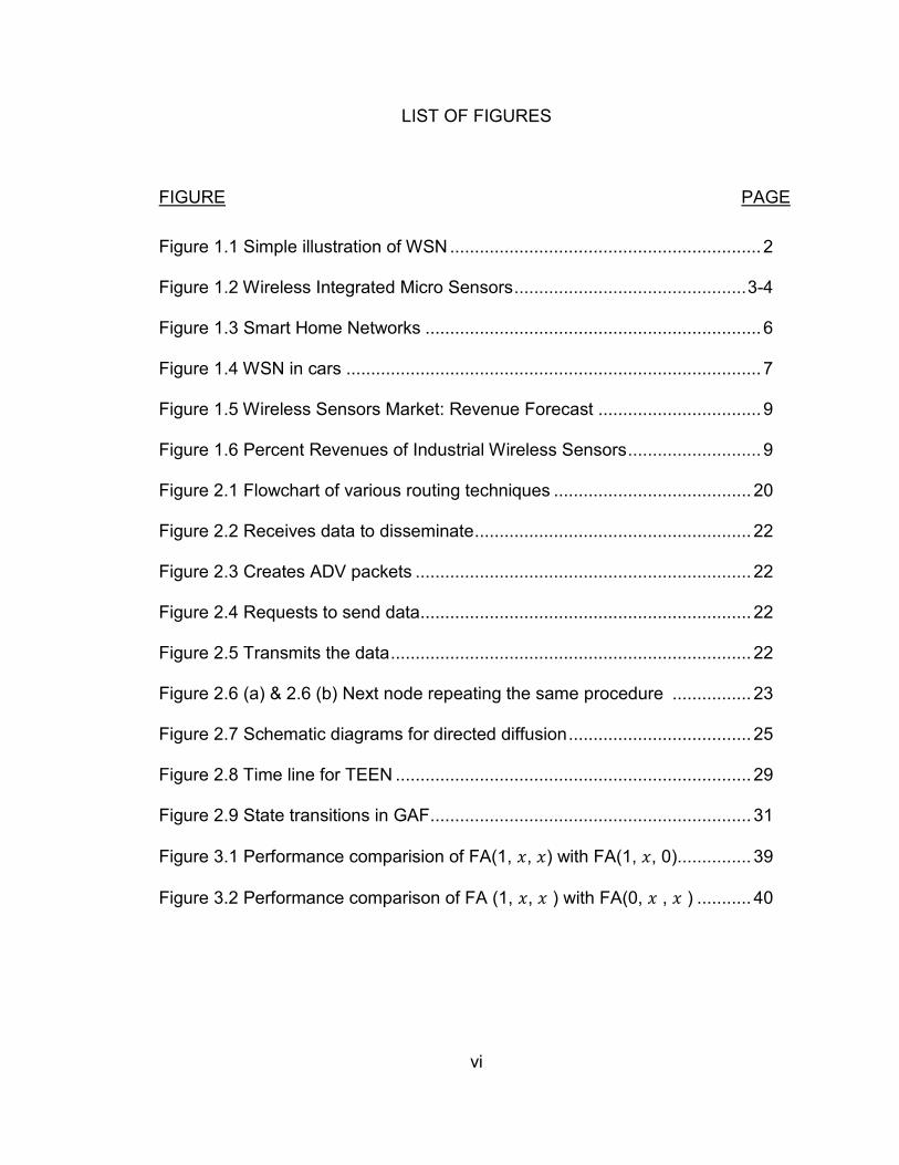
integrating complete systems on a single chip which makes it more cost efficient.
The Figure 1.1 shows a simple illustration of wireless sensor networks (WSNs)
Figure 1.1 Simple illustration of WSN.
1.1 EVOLUTION OF WSNs
In 1996, UCLA and the Rockwell Science Center produced the Low Power
Wireless Integrated Micro sensors (LWIMs). In 1998, the same team developed a

3
second generation sensor node although relatively powerful processing and
communication capabilities is offered by WINS, other research efforts focus on
developing smaller and cheaper nodes with less power consumption. In 1999,
UC Berkeley’s Smart Dust project released the first node, WeC, in their product
family of motes (Figure 1.3(a)). WeC was modeled with 8-bit, 4 MHz Atmel
microcontroller (512 bytes RAM and 8 KB ash memory), consuming 15mW active
power and 45 mW sleeping power. In 2001, Mica family was released along this
line, which still used an 8-bit 4 MHz microcontroller (ATmega103L), in terms of
memory and radio; it produced enhanced capabilities when compared with
preceding products. In order to reduce the standby current, the sequence to
Mica, Mica2 and Mica2Dot were built with an ATmega128 microcontroller in
2002. They provided improved radio modules with more selections for frequency
range, and by using FSK modulation increased resilience to noise. The Figure
1.2 shows the WeC, Mica, Telos and Spec modules [3].
(a) WeC
(b) Mica Family

4
(c) Telos
(d) Spec Prototype
Figure 1.2 Wireless Integrated Micro Sensors
The architectures of all the above mentioned sensors are based on batteries.
Techniques for energy scavenging from the environment have been an attractive
research field due to the slow advancement in battery capacity. In 2003, the first
radio transmitter, PicoBeacon (Figure 1.5), which is presented by the Berkeley
Wireless Research Center (BWRC) is purely powered by solar and vibration
energy sources [3].
1.1.1 Wireless Networking Technologies:
The development of WSNs relies also on wireless networking technologies apart
from hardware technologies. In 1997, the first standard for wireless local area
networks (WLANs), the 802.11 protocol was introduced. By increasing the data
rate and CSMA/CA mechanisms for medium access control (MAC), it got
upgraded to 802.11b. Routing techniques in wireless networks are another
important research direction for WSNs above the physical and MAC layers.
5
Actually, the existing routing protocols for wireless ad hoc networks or wireless
mobile networks are the early routing protocols in WSNs. Due to the high power
consumption, these protocols, including DSR and AODV, are hardly applicable to
WSNs [3]. Therefore scaling down the power consumption is another area where
there are ample research opportunities. In the near future, the era of WSNs is
highly anticipated.
1.2 APPLICATIONS
The applications in WSNs are generally classified into 2 categories,
namely Data Gathering Applications and Complex Computational Applications.
1.2.1 Data Gathering Applications:
The primary goal of these applications is to gather information of a
relatively simple form, such as temperature and humidity, from the operating
environment. Environmental monitoring and habitat study applications also
belong to this class [3].
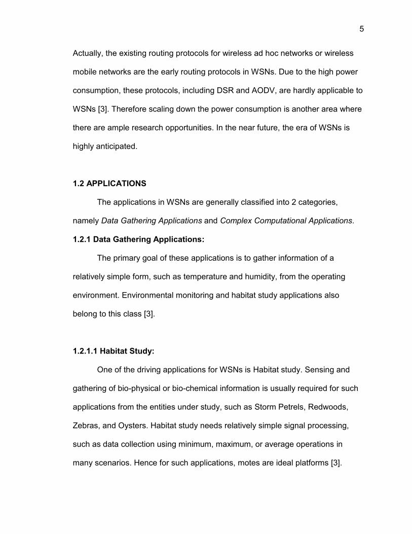
1.2.1.1 Habitat Study:
One of the driving applications for WSNs is Habitat study. Sensing and
gathering of bio-physical or bio-chemical information is usually required for such
applications from the entities under study, such as Storm Petrels, Redwoods,
Zebras, and Oysters. Habitat study needs relatively simple signal processing,
such as data collection using minimum, maximum, or average operations in
many scenarios. Hence for such applications, motes are ideal platforms [3].

6
1.2.1.2 Environmental Monitoring:
Environment monitoring is another field where WSNs have been used to a
greater extent, some of the best examples are, forest fire alarm, landscape
flooding alarm, soil moisture monitoring, micro climate and solar radiation
mapping, and environmental observation and forecasting in rivers [3]. All the
above examples are mostly large scale applications, smart homes can be
considered as a example of a small scale environmental monitoring. Driven by
emerging standards, increasing energy costs, and advances with Wireless
Sensor Networking, the “smart home” is becoming a reality for the mass market.
Figure 1.3 Smart Home Networks [4]
The Figure 1.3 shows how networks of various sorts might interact in the
smart home environment. The BACnet protocol has been developed by the
7
building automation industry to provide a standard for interconnecting networks
for building sensing and control [1].
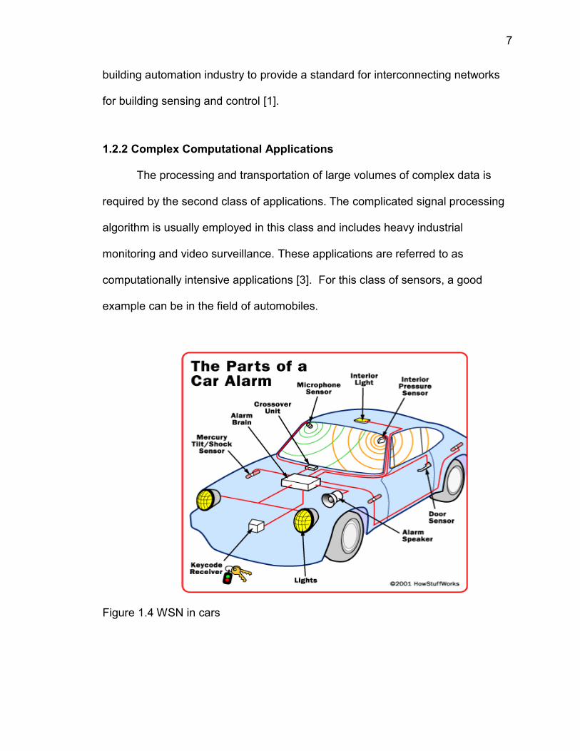
1.2.2 Complex Computational Applications
The processing and transportation of large volumes of complex data is
required by the second class of applications. The complicated signal processing
algorithm is usually employed in this class and includes heavy industrial
monitoring and video surveillance. These applications are referred to as
computationally intensive applications [3]. For this class of sensors, a good
example can be in the field of automobiles.
Figure 1.4 WSN in cars

8
The automobile application of wireless sensor networks comprises a
challenge to be encountered in this endeavor; during an automobile journey, we
believe a wireless sensor system is capable to collect process and supply
several types of technical information to the user. Acceleration and fuel
consumption, identification of wrong tires pressure value, acknowledgment of
illumination failures (turn lights, brake lights, front lights, and register plate lights),
and determination of the vital signals of the driver are few examples of it [5].
1.3 MARKET TRENDS
Wireless sensor networks market size was approximately $5billion in 2006
and $8billion in 2007, which according to the Wireless Research Group. More
than 700 million units were expected to grow by 2007, catching up with the
number of wireless handsets. More than half of the total market will be
constituted by building and industrial automation, two of Dust Networks’ primary
application.
9
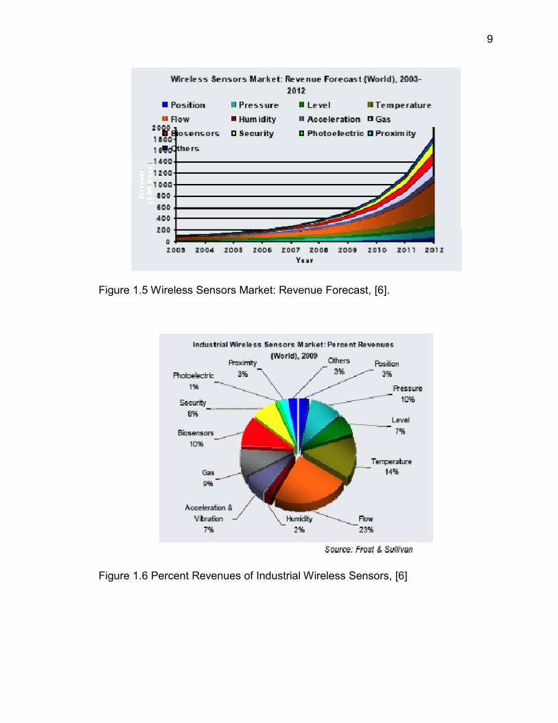
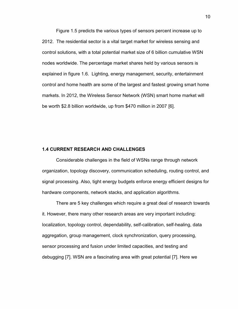
Figure 1.5 Wireless Sensors Market: Revenue Forecast, [6].
Figure 1.6 Percent Revenues of Industrial Wireless Sensors, [6]
10
Figure 1.5 predicts the various types of sensors percent increase up to
2012. The residential sector is a vital target market for wireless sensing and
control solutions, with a total potential market size of 6 billion cumulative WSN
nodes worldwide. The percentage market shares held by various sensors is
explained in figure 1.6. Lighting, energy management, security, entertainment
control and home health are some of the largest and fastest growing smart home
markets. In 2012, the Wireless Sensor Network (WSN) smart home market will
be worth $2.8 billion worldwide, up from $470 million in 2007 [6].
1.4 CURRENT RESEARCH AND CHALLENGES
Considerable challenges in the field of WSNs range through network
organization, topology discovery, communication scheduling, routing control, and
signal processing. Also, tight energy budgets enforce energy efficient designs for
hardware components, network stacks, and application algorithms.
There are 5 key challenges which require a great deal of research towards
it. However, there many other research areas are very important including:
localization, topology control, dependability, self-calibration, self-healing, data
aggregation, group management, clock synchronization, query processing,
sensor processing and fusion under limited capacities, and testing and
debugging [7]. WSN are a fascinating area with great potential [7]. Here we
11
would like to discuss briefly about the key challenges and our motivation towards
this theses work.
1.4.1 Information Processing
In any Wireless Sensor Networks (WSNs), we have 2 fundamental
processes, they are: Information processing and Information routing. Information
processing typically deals with sensing data, fusing data, query processing and
moving data. Information processing can be classified into three main categories,
including energy aware information processing algorithms design, space time
signal processing algorithms and networked information processing algorithms
[8].
1.4.1.1 Energy aware information processing algorithms design
The sensor nodes in WSNs are energy constrained and has a finite
lifetime. It would be highly desirable to carry out the information processing
algorithms in an energy aware manner. In order to make energy efficient
information processing the tradeoff between computational accuracy and energy
requirement of the algorithm on a single node should be determined. Then to
maximize the computational quality for a given energy constraint, we need break
down the algorithm into multiple tasks and distribute it among a group of nodes,
so that the energy consumption will be balanced among multiple nodes, and the
overall lifetime will be prolonged. It is a major division in Information processing
which opens a large area for research [8].

12
1.4.1.2 Space Time signal processing algorithms
An important aspect in the sensed region is that, always there exists a
time varying, space-time signature field that may be sensed by multiple nodes.
Individual nodes, however, only provide spatially local information. This
necessitates collaboration between nodes to process the space-time signal to
extract useful information such as the position of the moving object [8].
1.4.2 Information Routing
While information routing facilitates joint information compression (or data
aggregation) by bringing together data from multiple sources, information
processing helps reduce the data volume to be routed. However, analyzing and
modeling the inter-relationship between information processing and routing is
very significant. In many situations, the task of finding a routing scheme in
association with joint compression for energy minimization turns out to be NP-
hard [3]. Essential data between nodes in the region must be exchanged for
information processing due to the limited communication and computational
capability of each node. The routing of data should reduce the communication
cost so as to save energy from the viewpoint of networking [3][8].
1.4.3 Network Management
In most cases, sensor data must be delivered within a specified time
based on which appropriate observations can be made or actions can be taken.

13
One key challenge is to handle network dynamics during the process of network
discovery and organization. These dynamics include fluctuation in channel
quality, failure of sensor nodes, variations in sensor node capabilities, and
mobility or diffusion of the monitored entity. Hence WSNs require autonomous
adaptation of network discovery and organization protocols based on the network
and situation, in order to deliver proper system functionality [3].
1.4.4 Security & Privacy
Ensuring the integrity and confidentiality of sensitive information is
achieved by crucial security. To do so, intrusion and spoofing of the networks
should be well protected. It is unsuitable to use the conventional encryption
techniques as the sensor node is constrained of computation and communication
capability. Lightweight and application-specific architectures are preferred
instead [3]. By broadcasting a high-energy signal, an adversary attempts to
disrupt the operation in case of denial-of service attack. The entire system could
be jammed, if the transmission is strong enough. More sophisticated attacks are
also possible: By violating the MAC protocol, the adversary can inhibit
communication, for instance by continuously requesting channel access or by
transmitting while a neighbor is also transmitting or with a RTS (request to- send)
[7]. Since components designed without security can become a point of attack,
every component must be integrated with security so as to achieve secure
system [7].

14
1.4.5 Energy Conservation
In WSNs, it is often infeasible or undesirable to re-charge sensor nodes or
replace their batteries once they are installed and configured. Thus, energy
conservation of sensor network becomes crucial for sustaining a sufficiently long
network lifetime [3]. The majority of current research focuses on ways to provide
full or partial sensing coverage in the context of energy conservation. In such an
approach, nodes are put into a dormant state as long as their neighbors can
provide sensing coverage for them [7]. Energy conservation can also be
achieved by employing smart routing algorithms that are generally referred to as
energy aware information processing and routing algorithms. There are number
of power reduction strategies for the sensor, some are listed below [9],
Turn power on to sensor only when sampling.
Turn power on to signal conditioning only when sampling sensor.
Only sample sensor when an event occurs.
Lower sensor sample rate to the minimum required by the application.
Implement an event-driven transmission strategy; only transmit data when
a sensor event occurs.
In spite of large number of existing strategies energy conservation still remains
one of the major challenges for the industry.
1.5 MY WORK
When we take a look at the existing challenges energy conservation of the
Wireless Sensor Networks seems to be a major road block. This work focuses on

15
addressing the energy conservation issues by coming up with a smart routing
algorithm which is completely aware of the existing energy issues, thereby
increasing the overall lifetime of the network. This work is split into 4 chapters;
the crux of each chapter is as follows,
CHAPTER 1: This chapter will introduce the basic concepts about the Wireless
Sensor Networks. It discusses the evolution of the WSN technology, its current
technology, etc. It also briefs the market trends and the extent to which WSN
plays a role in world economy. Finally here we discuss the challenges involved to
design an optimized WSN.
CHAPTER 2: Routing characteristics, challenges and key issues of routing are
discussed in this section. And a brief detail of different routing protocols are
discussed here.
CHAPTER 3: In this section, linear programming formulation, existing algorithm
and proposed algorithm is discussed. It is followed by examples to compare the
proposed algorithm with existing algorithm. Then finally small window and large
window information generation windows are analyzed.
CHAPTER 4: In this section we discuss the results obtained by using our
algorithm and also we compare our results with the results from flow
augmentation algorithm proposed in [21]. Finally we summarize our work and
propose ways to extend our work in future in the conclusion part.

16
CHAPTER 2
ROUTING PRTOCOLS FOR SENSOR NETWORKS
Wireless sensors are small, inexpensive, low power devices which are
deployed in large numbers over an area in an ad hoc fashion. Each sensor node
has a limited battery life, limited gaze of the environment and limited processing
power. A large number of such nodes which can co-ordinate amongst
themselves give them huge advantage over centralized single sensor based
techniques. Wireless Sensor networks have severe resource constraints,
asymmetric many to one data flow and unreliable network nodes. Thus their
primary objective is for energy conservation and prolonging network lifetime,
which overlooks at performance, bandwidth and QoS to optimize the primary
goals. Several current protocols are based on energy efficient routing.
Routing protocols, designed for sensor networks, must accomplish high
reliability in the proximity of individual or patterned node. There has to be multiple
paths to relay the data from source node to the destination node in order to
achieve robustness. Sensor nodes are constrained in energy supply and
recharging sensor nodes is normally impractical when they are out of power,
therefore, energy saving is an important design issue in sensor networks. While
the objective of traditional networks is to achieve high quality of service

17
provisions, sensor network protocols must focus primarily on power conservation
to maximize the network lifetime. Many recent research efforts are focused on
how to improve energy efficiency of sensor networks. Flooding the network is a
highly expensive operation with respect to energy consumption and should be
avoided [10].
2.1 ROUTING CHARACTERISTICS
In the network, consumption of energy is mainly due to the Routing of
data; efficient routing protocols can reduce the energy consumption drastically. In
sensor networks, routing protocols can be classified based on number of
criterions such as proactive vs. reactive routing, hierarchical vs. non-hierarchical
routing, etc. In proactive routing, the data path is setup in advance and suitable
routing table is maintained. While in reactive routing, the routing tables and paths
are created on the fly as and when required. Either source or destination can
initiate the routing. Below we discuss a few characteristics of a good routing
protocol.
The important characteristics of a “good” routing protocol are as follows
[11].
Simplicity: due to the limited computation capabilities of nodes, the
protocol used should not be too large or complex. Memory requirements
and the amount of overhead it generates for routing should be reduced,
which refers to minimizing the communication and state of the protocol.
Energy awareness: the battery lifetime of sensor nodes is limited. For a

18
protocol to avoid nodes that are heavily depleted or use energy-rich
nodes, it should have the knowledge of the current energy use and the
battery charge.
Adaptability: Sensor nodes are inherently unreliable. When there is a
network change as a result of node failure, the system should be able to
adapt to it.
Scalability: Routing must scale gracefully when the sensor networks are
scaled to hundreds and thousands of nodes. The size of the routing table
that are maintained and how they scale with the number of nodes in the
network is the key part.
2.2 ROUTING CHALLENGES AND KEY ISSUES
Despite enormous applications of WSNs, sensor nodes are constrained in
bandwidth and energy supply. Such constraints combined with a typical
deployment of large number of sensor nodes have posed many challenges to the
design and management of sensor networks [12].
Sensor networks pose unique constraints in designing protocols and
hardware for them. The major challenges faced are:
(a)Nature of deployment: Sensor networks are to be deployed in an Ad-hoc
fashion with a little correlation in the nodes placement. The detection of network
and its distribution is left to the nodes. In order to sustain the hardships of
deployment in hostile conditions, the hardware should be rough enough.
(b)Self configuration: The system must be completely self configurable as the
19
nodes are deployed to work in an environment of unattended human intervention.
(c)Reliability: A high reliability is expected on each link as the relayed data has to
cross over multiple hops, or else the possibility of data reaching its destination is
very low. (d)Quality of Service: Few applications demand packet delivery to be
reached to its destination by specific time limit. Developing protocols for such
applications is difficult and challenging one, as the degree of uncertainty in WSN
is very high. (e)Mobility: Routing gets more difficult if either the message source
or destination or both are moving. To solve this, the routing table has to be kept
updating continuously or find proxy nodes which are responsible for keeping
track of where nodes are. If a node moves away from its original location further,
then the proxy node may also vary for a given node. (f)Security: Routing
algorithms are susceptible to a variety of attacks, including selective forwarding,
black hole, Sybil, replays, wormhole and denial of service attacks. (g)Congestion:
In WSN, Packet losses and resending of data resulting from congestion cost
precious energy and shorten the lifetime of sensor nodes. However, congestion
is more dominant with larger systems that might process audio, video and have
multiple base stations.
2.3 ROUTING TECHNIQUES
Many algorithms have been proposed for the problem of data routing in
sensor networks. The characteristics of sensor nodes along with the application
and architecture requirements have been considered in developing these routing
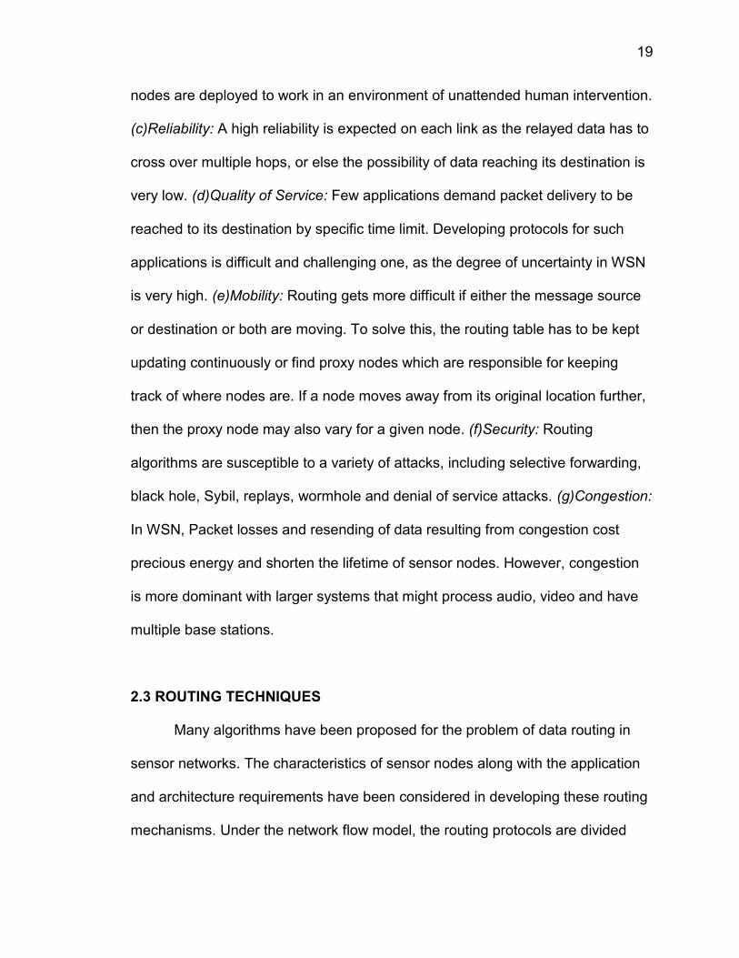
mechanisms. Under the network flow model, the routing protocols are divided
20
into flat-routing, hierarchical-based and location-based routing. In flat-based
routing, no distinct roles of each node, all nodes are equal in functionality. In
hierarchical-based routing, each node is distinct from one another and is of
different functionality. In location-based routing, the locations of the nodes are
manipulated to route the data.
Figure 2.1 Flowchart of various routing techniques.
2.3.1 SPIN (Sensor Protocol for Information via Negotiation)
It is a negotiation based data dissemination protocol where unlike the
other cases we want to send data to all nodes treating all nodes in the network
as sink nodes. The design goal is to avoid the drawbacks of flooding protocols by
utilizing data negotiation and resource-adaptive algorithms [13].
21
2.3.2 Drawbacks in classical flooding of networks
2.3.2.1 Implosion:
The network wastes resources by sending multiple packets of same data
item i.e. node always sends a data packet to its entire neighbor without
considering whether it has already transmitted the same packet earlier. The
reason for this is lacking of mechanisms to uniquely identify a data item.
2.3.2.2 Overlap:
When more than one sensor monitor events, then the sensor network
might form a geographically overlapping regions leading to situation when a
common node receives multiple copies of a piece of data.
2.3.2.3 Resource Blindness:
Nodes do not adapt their behavior with change in energy level as it is
unaware of the resource. By implementing negotiation based data transfer and
resource-adaptation, SPIN overcomes these limitations. Before transmission,
nodes negotiate to transfer unique data. This overcomes implosion. SPIN
protocol name their data using high-level data descriptors, called meta-data.
They use meta-data negotiations to discard the transmission of redundant data
throughout the network. Inclusion of a resource manager which is polled before
transmitting introduces resource awareness in the nodes.
22
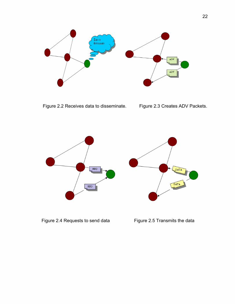
Figure 2.2 Receives data to disseminate. Figure 2.3 Creates ADV Packets.
Figure 2.4 Requests to send data Figure 2.5 Transmits the data
23
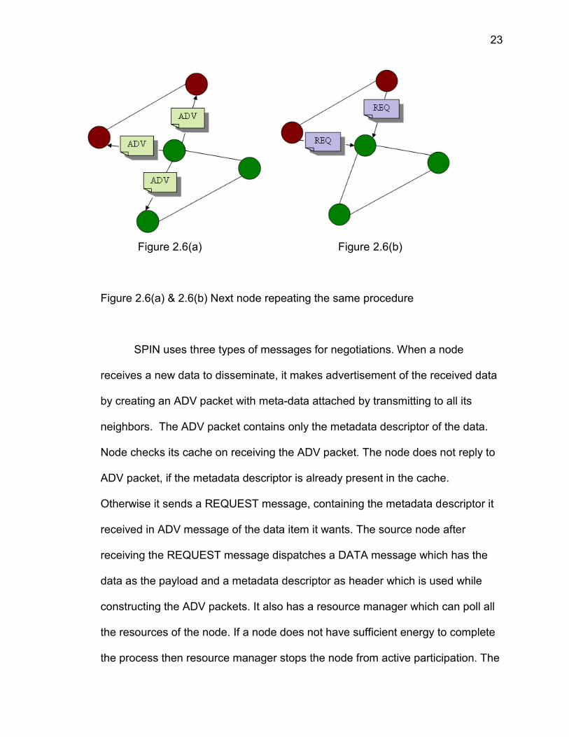
Figure 2.6(a) Figure 2.6(b)
Figure 2.6(a) & 2.6(b) Next node repeating the same procedure
SPIN uses three types of messages for negotiations. When a node
receives a new data to disseminate, it makes advertisement of the received data
by creating an ADV packet with meta-data attached by transmitting to all its
neighbors. The ADV packet contains only the metadata descriptor of the data.
Node checks its cache on receiving the ADV packet. The node does not reply to
ADV packet, if the metadata descriptor is already present in the cache.
Otherwise it sends a REQUEST message, containing the metadata descriptor it
received in ADV message of the data item it wants. The source node after
receiving the REQUEST message dispatches a DATA message which has the
data as the payload and a metadata descriptor as header which is used while
constructing the ADV packets. It also has a resource manager which can poll all
the resources of the node. If a node does not have sufficient energy to complete
the process then resource manager stops the node from active participation. The
24
node does not reply to ADV if it has no sufficient energy left in it.
The protocol have been compared with three standard protocols namely
(a)Classical flooding: Each sensor on receiving data, forwards it to all its
neighboring nodes without inspecting whether it has already transmitted a copy
or not. (b)Gossiping: The node selects a random neighbor to transmit the
received data, which picks another random neighbor to forward the data to and
so on, instead of indiscriminately forwarding as in classical flooding to all its
neighbors [12]. (c)Ideal case: Here data is sent to all the nodes on the shortest
path from the source. For this purpose we can use IP level multicasting, etc.
The result obtained indicates that SPIN gives much better performance then
classical flooding and gossiping. In comparison to classical flooding and
gossiping, the energy dissipation is low. For a simulation with fixed amount of
energy the SPIN protocol was able to disseminate 73%, when ideal method did
85%, flooding did 53% and gossiping dissipated only 38% of data.
2.3.3 Directed Diffusion
Directed diffusion is another data dissemination protocol in which
attributes value pairs name the data generated by the nodes. The routes are
determined upon request as this is a destination-initiated reactive routing
technique. Throughout the network, for named data a sensing task or interest is
propagated by a node and data matching this interest is then sent towards this
node. By exchanging messages between neighboring nodes within some
distance helps in determining the propagation of data and its aggregation at
25
intermediate nodes on the way to the request originating node. Tasks are
described by the list of attribute-value pairs. This description is called an interest.
In a similar way, naming is done for the response data to such an interest. The
sink node which is the querying node broadcasts its interest message repeatedly
to all of its neighbors. Each item of an interest cache of all the nodes
corresponds to a different interest. No information about the sink node is
contained in these entries [14][15].
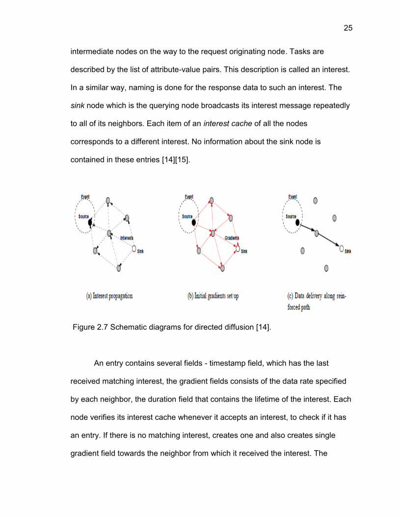
Figure 2.7 Schematic diagrams for directed diffusion [14].
An entry contains several fields - timestamp field, which has the last
received matching interest, the gradient fields consists of the data rate specified
by each neighbor, the duration field that contains the lifetime of the interest. Each
node verifies its interest cache whenever it accepts an interest, to check if it has
an entry. If there is no matching interest, creates one and also creates single
gradient field towards the neighbor from which it received the interest. The
26
timestamp and the duration fields are updated if already an interest exists. When
a gradient is expired, it is removed from its interest entry. The data rate as well
as the direction in which the event has to be transmitted is specified by a
gradient. The nodes receiving interest from its neighbors think that node as the
originating node but in fact it is transmitting the received interest. Hence, diffusion
of interests occurs through the network. A node first examines its interest cache
for a matching interest entry whenever it detects an event. If it finds one, then
even samples are generated at the highest rate and which is computed from the
event rates of outgoing gradients. All of its neighboring nodes which have
gradients receive the event description. Hence, when an event is noticed, the
sink starts receiving low data rate events, possibly along multiple paths. One
particular neighbor is reinforced by the sink to receive the better quality events.
This would probably lead to a multiple reinforced paths in which case, the better
performing path is withhold and by timing out all the high data rate gradients in
the network , the other paths are negatively reinforced while repeatedly
reinforcing the selected path.
2.3.4 LEACH (Low-Energy Adaptive Clustering Hierarchy)
LEACH is an adaptive clustering-based protocol using randomized
rotation of cluster-heads to evenly distribute the energy load among the sensor
nodes in the network. The data will be collected by cluster heads from the nodes
in the cluster and after processing and data aggregation forwards it to base
station [16][17]. The three important features of LEACH are:

27
Localized co-ordination and control for cluster setup.
Randomized cluster head rotation.
Local compression to reduce global data communication.
By forming clustering, the energy usage is low within the cluster but drains the
energy resource for the cluster head. The cluster heads need to be more
powerful than other common nodes of the networks of fixed cluster heads in
order to perform maximum long distance communication [16][17].
LEACH’s operation is divided into rounds. Each round can be further divided into
the following steps:
Advertisement phase: With a certain probability, each node accepts to
become a cluster head. The selected node advertises its cluster head
status and depending on the signal quality, all the other nodes choose one
of the clusters.
Cluster setup phase: Each node informs a particular cluster head about its
will to join. Out of multiple advertisement messages, a node selects one
cluster head depending on criterions such as proximity, signal to noise
ratio, etc.
Schedule creation: For data transmission, each member of a cluster head
follows the assigned TDMA scheduling. If nodes do not have any data to
transmit then they can enter into sleep mode/close radio mode [16][17].
28
Data transmission: The cluster head performs aggregation and
compression of received data from all of its member nodes, which
transmitted the data during allotted TDMA schedule [16][17].
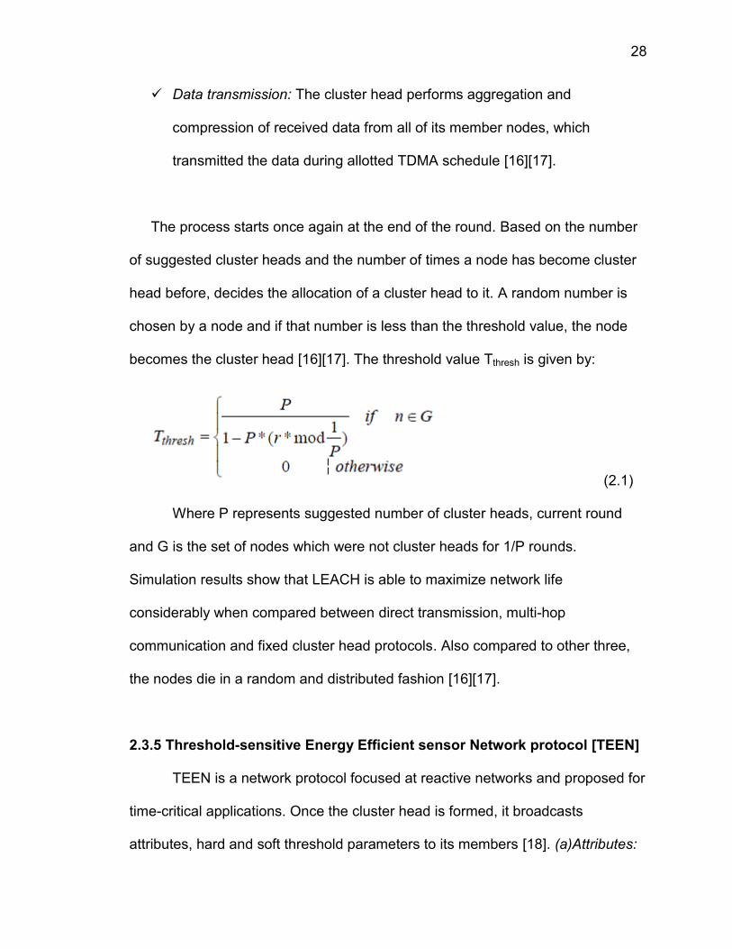
The process starts once again at the end of the round. Based on the number
of suggested cluster heads and the number of times a node has become cluster
head before, decides the allocation of a cluster head to it. A random number is
chosen by a node and if that number is less than the threshold value, the node
becomes the cluster head [16][17]. The threshold value Tthresh is given by:
(2.1)
Where P represents suggested number of cluster heads, current round
and G is the set of nodes which were not cluster heads for 1/P rounds.
Simulation results show that LEACH is able to maximize network life
considerably when compared between direct transmission, multi-hop
communication and fixed cluster head protocols. Also compared to other three,
the nodes die in a random and distributed fashion [16][17].
2.3.5 Threshold-sensitive Energy Efficient sensor Network protocol [TEEN]
TEEN is a network protocol focused at reactive networks and proposed for
time-critical applications. Once the cluster head is formed, it broadcasts
attributes, hard and soft threshold parameters to its members [18]. (a)Attributes:
29
It is a set of physical parameters that the user is interested in obtaining [18].
(b)Hard Threshold (HT): It is a threshold value for the sensed attribute [18].
(c)Soft Threshold (ST): It is a small change in the value of the sensed attribute.
The hard threshold parameter allows the nodes to transmit only when the sensed
attribute is in the range of interest, which reduces the number of transmissions.
Soft threshold parameter check on the sensed attribute value and if there is little
or no vary in the sensed attribute, soft threshold parameter reduces the number
of transmissions further by eliminating all the transmissions which might have
occurred [18].
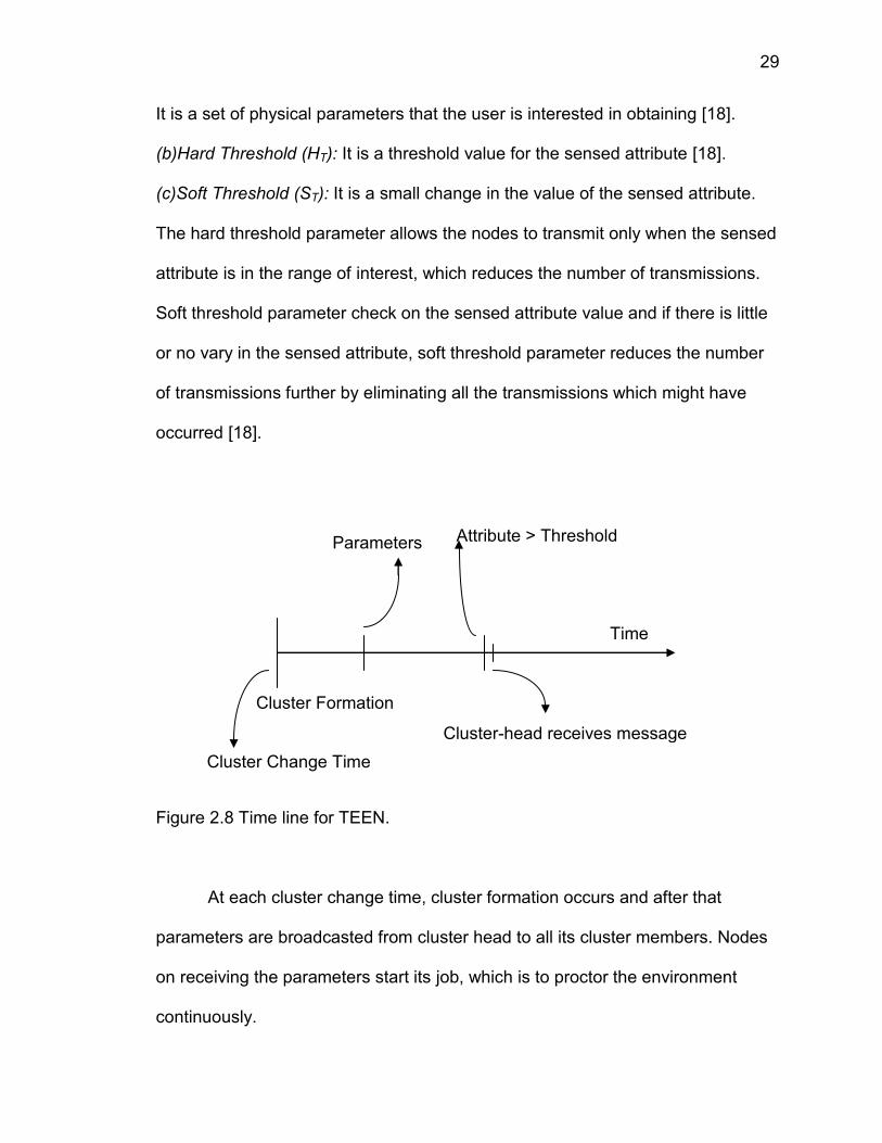
Figure 2.8 Time line for TEEN.
At each cluster change time, cluster formation occurs and after that
parameters are broadcasted from cluster head to all its cluster members. Nodes
on receiving the parameters start its job, which is to proctor the environment
continuously.
Attribute > Threshold
Cluster-head receives message
Parameters
Cluster Change Time
Cluster Formation
Time
30
If the sensed attribute is greater than the obtained hard threshold parameter,
the node switch on its transmitter and transmits the sensed data to its cluster
head for the first time. Sensed attribute is stored in an internal variable in the
node, known as sensed value (SV). After that in order for a node to transmit its
sensed data, the following conditions have to be met:
Current value of the sensed attribute should be greater than the hard
threshold.
Current value of the sensed attribute should differ from SV by an amount
equal to or greater than the soft threshold.
The key features of TEEN include its ability of transmitting data almost
instantaneously for time critical applications. Message transmission consumes
more energy than data sensing, so the energy consumption in this scheme is
potentially less than the proactive networks. The user can vary the attributes as
required, as it is broadcasted afresh at every cluster change time. And also, soft
threshold can be changed. The main drawback of this scheme is that, the nodes
will never communicate to the user, if the thresholds are not reached.
2.3.6 Geographic Adaptive Fidelity (GAF)
GAF is an energy-aware location-based routing algorithm designed
primarily for mobile ad hoc networks, but may be applicable to sensor networks
as well. The network area is divided into fixed zones to form a virtual grid, and
nodes inside each zone work together to perform different roles. For example,
31
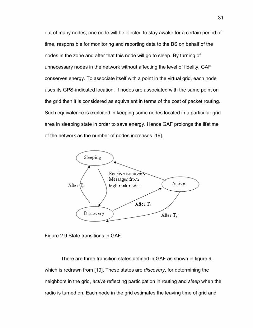
out of many nodes, one node will be elected to stay awake for a certain period of
time, responsible for monitoring and reporting data to the BS on behalf of the
nodes in the zone and after that this node will go to sleep. By turning of
unnecessary nodes in the network without affecting the level of fidelity, GAF
conserves energy. To associate itself with a point in the virtual grid, each node
uses its GPS-indicated location. If nodes are associated with the same point on
the grid then it is considered as equivalent in terms of the cost of packet routing.
Such equivalence is exploited in keeping some nodes located in a particular grid
area in sleeping state in order to save energy. Hence GAF prolongs the lifetime
of the network as the number of nodes increases [19].
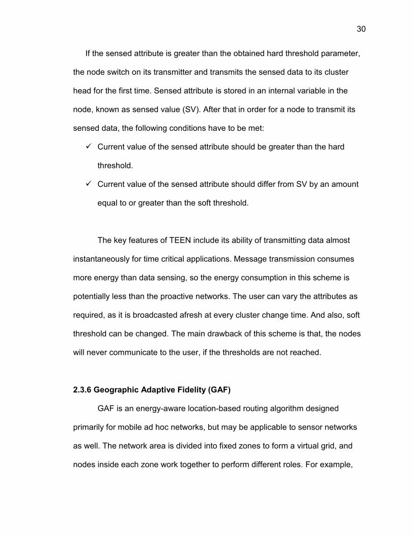
Figure 2.9 State transitions in GAF.
There are three transition states defined in GAF as shown in figure 9,
which is redrawn from [19]. These states are discovery, for determining the
neighbors in the grid, active reflecting participation in routing and sleep when the
radio is turned on. Each node in the grid estimates the leaving time of grid and
32
sends this to its neighbors to handle the mobility. In order to keep the routing
fidelity, sleeping neighbors adjust their sleeping time accordingly. One of the
sleeping nodes becomes active much before the leaving time of the active node
expires. GAF is implemented both for non-mobility (GAF-basic) and mobility
(GAF-mobility adaptation) of nodes. GAF always keeps a representative node in
active mode for each region on its virtual grid to ensure network connectivity.
Simulation results show that GAF performs at least as well as a normal ad hoc
routing protocol in terms of latency and packet loss and increases the lifetime of
the network by saving energy [19].
2.3.7 Geographic and Energy Aware Routing (GEAR)
The GEAR protocol uses energy aware and geographically-informed
neighbor selection heuristics to route a packet towards the targeted region. The
key idea in this scheme is to consider only a certain region to transmit the
interests rather than sending the interests to the whole network as in directed
diffusion. GEAR can conserve more energy than directed diffusion with this idea
[20].
In this scheme, each node keeps an estimated cost and a learning cost of
reaching the destination through its neighbors. The combination of residual
energy and distance to destination is the estimated cost. The learned cost is a
refinement of the estimated cost that accounts for routing around holes in the
network. If a node does not have any nearby neighbor to the targeted region than
itself, a hole appears. When there are no holes, the estimated cost is equal to

33
the learned cost. The learned cost is propagated one hop back every time a
packet reaches the destination so that route setup for next packet will be
adjusted. There are two phases in the algorithm [20]:
Forwarding packets towards the target region: A node checks its
neighbors on receiving a packet to see if there is a neighbor that is closer
to the targeted region than itself. The nearest neighbor to the targeted
region is selected as the next hop, if there is more than one neighbor. If
they are all further than the node itself, then there is a hole. In this case,
one of the neighbors is picked to forward the packet based on the learning
cost function. This choice can then be updated according to the
convergence of the learned cost during the delivery of packets.
Forwarding the packets within the region: If the packet has reached the
region, it can be diffused in that region by either recursive geographic
forwarding or restricted flooding. Restricted flooding is better, if the
sensors are not densely deployed. Recursive geographic flooding is more
energy efficient than restricted flooding when the sensors are densely
deployed.
34
CHAPTER 3
METHODOLOGY
In this section, we first summarize the maximum lifetime routing problem,
which is formulated as a linear programming problem. It is followed by a
discussion on the flow augmentation algorithm and proposed heuristic in this
paper with examples. Then a comparison is made between smaller windows
against larger windows.
3.1 MAXIMUM LIFETIME ROUTING PROBLEM
Consider a wireless sensor network with N nodes. Let represent the set
of immediate neighbors of node i ∈ N, indicates the average power consumed
for data transmission from node i to node j and be the initial battery level of
node i. Let there be multiple commodities, where a set of source node and
destination node forms a commodity. We have, for each commodity c ∈ C, a set
of origin nodes where information is generated at node i with rate (c) and a
set of destination nodes among which any node can be reached in order for
the information transfer of commodity c to be considered done. Let
be the
traffic generated at node i and destined for node j and be the amount of data
that needs to be transmitted from node i to node j.
35
The main objective is to maximize the system lifetime which is by
definition the time of the first node death and is equivalent to maximizing the total
amount of information transmission under a fixed information generation rates.
The above problem can be shown as a linear programming problem. Given the
amount of information generated
at each origin nodes for each
commodity c, the problem of maximizing the system lifetime is analogous to
linear programming problem which is as shown below:
Maximize
s.t. ∀i ∈ N, ∀j ∈ , ∀c ∈ C,
* ≤ (3.1)
= + (3.2)
From equation (3.2), we can see that the total amount of data that node i
sends is the amount of data that this node generates plus the amount of data it
has received from its predecessor nodes.
3.2 FLOW AUGMENTATION ALGORITHM
The authors in [21] proposed a heuristic called the flow augmentation
algorithm for fixed information generation rates and arbitrary information
generation rates, which aims at maximizing the system lifetime of a wireless
sensor networks. In this paper, we concentrate only on fixed information
generation rates and the description of the algorithm is as given below.

36
Algorithm FA( , , )
At each iteration,
1. Calculate the shortest cost path for each commodity c with cost of link (i, j)
given by
=
+
(3.3)
If there is enough residual energy for a packet, i.e., if - >0. The path cost
is given by the sum of the link costs.
2. If any of the commodities cannot find a path to its destination then stop.
Otherwise continue.
3. Augment λ (c) on each shortest cost path of its commodity and update the
residual energy accordingly.
4. Goto 1.
In the above description, λ is the augmentation step size which is
equivalent to the amount of information routed between routing information
updates and the cost function for each link described above in the algorithm
will be defined in the following section.
3.3 COST FUNCTION
The main objective is to ensure that node and network life is prolonged by
properly managing the power conservation of a node and sharing the cost of
routing packets carefully [23].
37
The process of choosing a path demands the knowledge about flow
requirements, characteristics, availability of resources in networks and evaluating
the quantity of resources that needs to be assigned to encourage the new flow
[24].
To achieve our objective of “maximum lifetime”, we should give
importance to all the nodes and ensure that no node must be penalized more
than any of the others, which is equivalent to the nodes with depleted energy
resources do not lie on many paths [23].
To implement this, several power-aware metrics that does result in
energy-efficient routes has been presented in [23] separately. The authors [21]
combined all these metrics into one and proposed a new link metric, which will
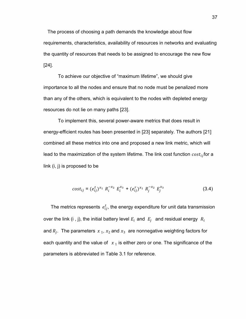
lead to the maximization of the system lifetime. The link cost function for a
link (i, j) is proposed to be
=
+
(3.4)
The metrics represents , the energy expenditure for unit data transmission
over the link (i , j), the initial battery level and and residual energy
and . The parameters , and are nonnegative weighting factors for
each quantity and the value of is either zero or one. The significance of the
parameters is abbreviated in Table 3.1 for reference.

38
Table 3.1 Meanings of the parameters in the Algorithm FA [21]
The above link cost, has been put up taking into consideration that
flow augmenting path should consider minimum total consumed energy path
when the network is new, should use up less resource and should stay away
from nodes with small residual energy [21].
Each link cost add up to form a path cost and out of many available paths
from source node to destination node of a commodity c ∈ C, the shortest cost
path is computed by the execution of shortest path algorithm. Distributed
Bellman-Ford algorithm is used in Flow augmentation algorithm and Dijkstra’s
shortest path algorithm is used in this proposed algorithm.
39
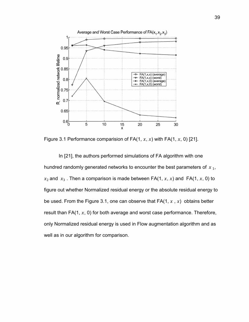
Figure 3.1 Performance comparision of FA(1, , ) with FA(1, , 0) [21].
In [21], the authors performed simulations of FA algorithm with one
hundred randomly generated networks to encounter the best parameters of ,
and . Then a comparison is made between FA(1, , ) and FA(1, , 0) to
figure out whether Normalized residual energy or the absolute residual energy to
be used. From the Figure 3.1, one can observe that FA(1, , ) obtains better
result than FA(1, , 0) for both average and worst case performance. Therefore,
only Normalized residual energy is used in Flow augmentation algorithm and as
well as in our algorithm for comparison.
40
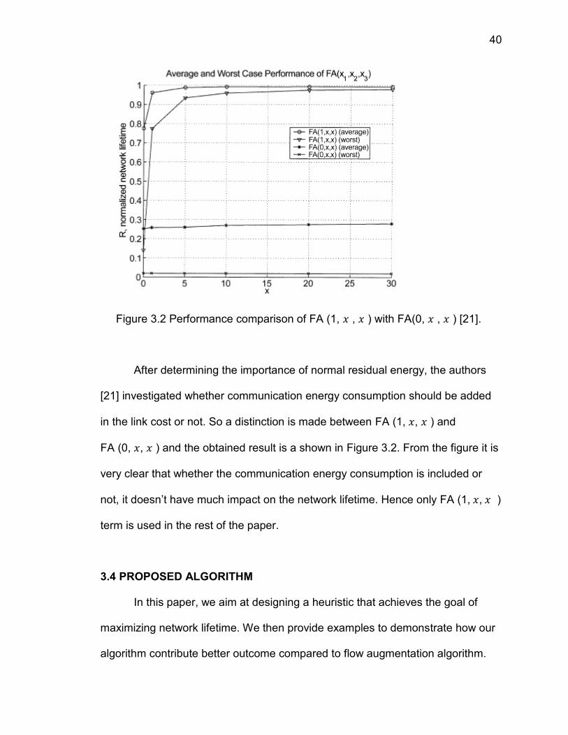
Figure 3.2 Performance comparison of FA (1, , ) with FA(0, , ) [21].
After determining the importance of normal residual energy, the authors
[21] investigated whether communication energy consumption should be added
in the link cost or not. So a distinction is made between FA (1, , ) and
FA (0, , ) and the obtained result is a shown in Figure 3.2. From the figure it is
very clear that whether the communication energy consumption is included or
not, it doesn’t have much impact on the network lifetime. Hence only FA (1, , )
term is used in the rest of the paper.
3.4 PROPOSED ALGORITHM
In this paper, we aim at designing a heuristic that achieves the goal of
maximizing network lifetime. We then provide examples to demonstrate how our
algorithm contribute better outcome compared to flow augmentation algorithm.
41
The algorithm is depicted for fixed information–generation rates.
We have come up with a heuristic, which targets to improve a heuristic
scheme proposed in [21]. Similarly to flow augmentation algorithm, at each
iteration our algorithm determine the shortest cost path from a source node o ∈
to its corresponding destination node for a commodity c ∈ C. The cost
function is same as that of the flow augmentation algorithm, but reception metric
is not included here since it is very negligible. Then information is relayed on the
calculated shortest cost path between source node o and destination node
by a magnitude of λ , where λ is augmentation step size which is equivalent
to the amount of information routed between routing information updates [21].
Routing information update is carried out after the residual energy is
updated at each node, which will vary the link costs. The defined method is
repeated until the time network partition occurs because of node failure.
However in our algorithm, the nodes are not mobile and the topology of the
network is static.
Hence obtained result is applicable for static networks. The energy
consumption at unintended receiver nodes and at the receivers during reception
is not included in the algorithm. Also energy consumption due to routing control
packets is not included in the model assuming that energy consumption is
dominated by the data packets.

42
Algorithm
1) For a commodity c ∈ C, calculate the shortest cost path with link cost (i, j)
given by
=
(3.5)
If and only if - >0. Summation of the each link cost will obtain the path
cost.
2) If a commodity c ∈ C cannot find a path to its destination then stop. Else
continue.
3) Augment λ on the calculated shortest cost path of a commodity and
update the residual energy accordingly.
4) Goto 1.
3.5 COMPARISON OF FA ALGORITHM AND PROPOSED ALGORITHM
Figure 3.3 Example to compare FA algorithm and proposed algorithm
43
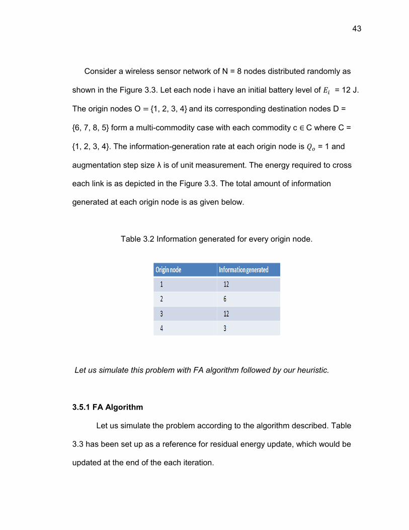
Consider a wireless sensor network of N = 8 nodes distributed randomly as
shown in the Figure 3.3. Let each node i have an initial battery level of = 12 J.
The origin nodes O = {1, 2, 3, 4} and its corresponding destination nodes D =
{6, 7, 8, 5} form a multi-commodity case with each commodity c ∈ C where C =
{1, 2, 3, 4}. The information-generation rate at each origin node is = 1 and
augmentation step size λ is of unit measurement. The energy required to cross
each link is as depicted in the Figure 3.3. The total amount of information
generated at each origin node is as given below.
Table 3.2 Information generated for every origin node.
Let us simulate this problem with FA algorithm followed by our heuristic.
3.5.1 FA Algorithm
Let us simulate the problem according to the algorithm described. Table
3.3 has been set up as a reference for residual energy update, which would be
updated at the end of the each iteration.
44
Table 3.3 Reference table for residual energy update
Initial Energy E1 E2 E3 E4 E5 E6 E7 E8
12 12 12 12 12 12 12 12
Residual
Energy
R1 R2 R3 R4 R5 R6 R7 R8
12 12 12 12 12 12 12 12
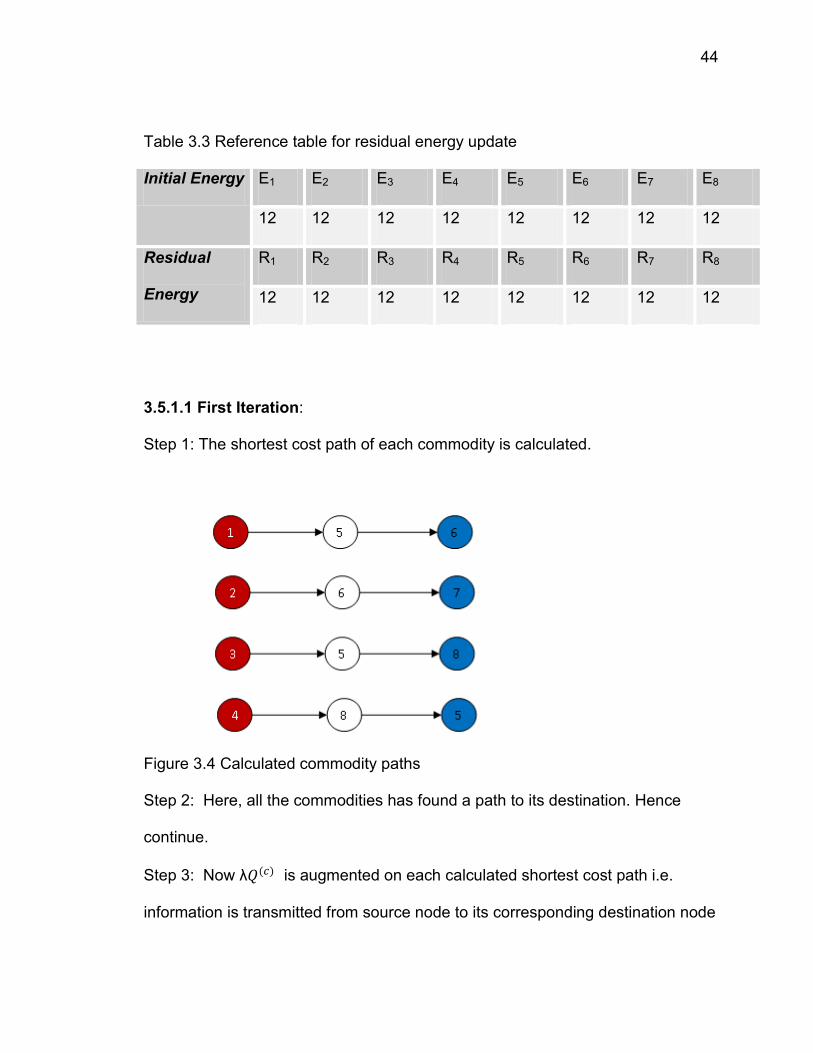
3.5.1.1 First Iteration:
Step 1: The shortest cost path of each commodity is calculated.
Figure 3.4 Calculated commodity paths
Step 2: Here, all the commodities has found a path to its destination. Hence
continue.
Step 3: Now λ is augmented on each calculated shortest cost path i.e.
information is transmitted from source node to its corresponding destination node
45
via the calculated shortest cost path. Now update the residual energy
accordingly.
Table 3.4 Residual energy update after first iteration
Initial Energy E1 E2 E3 E4 E5 E6 E7 E8
12 12 12 12 12 12 12 12
Residual
Energy
R1 R2 R3 R4 R5 R6 R7 R8
10 8 9 9 6 11 12 9
Step 4: Continue to step 1.
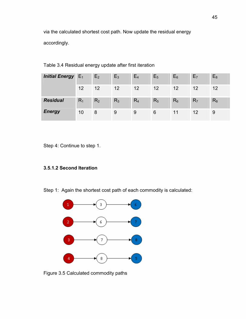
3.5.1.2 Second Iteration
Step 1: Again the shortest cost path of each commodity is calculated:
Figure 3.5 Calculated commodity paths

46
Step 2: There is a path for all the commodities to its corresponding destination.
Hence continue.
Step 3: Augmenting λ on the calculated paths and Update the residual
energy accordingly.
Table 3.5 Residual energy update after second iteration.
Initial Energy E1 E2 E3 E4 E5 E6 E7 E8
12 12 12 12 12 12 12 12
Residual
Energy
R1 R2 R3 R4 R5 R6 R7 R8
9 4 X 6 6 10 9 6
While augmenting λ on each shortest cost path, source node 1
transmits the assigned packet to its destination node (node 6) successfully.
Similarly, node 2 delivers its packet to node 7 with ease. A real problem
occurred on transmitting data from node 3 to node 8 as it could not make through
in transmitting data as calculated in step 1.The packet got dropped due to
inadequate energy at node 3.
Then how did step 2 pass over declaring all commodities has found a
path? After first iteration, node 3 had a residual energy of 9 J. Node 1 selected
node 3 as via node to node 6. It requires 5 J of energy for node 3 to relay the
received packet from node 1 to node 6 as depicted in Figure 3.3, which made the
residual energy of node 3 to 4 J although the residual energy update happens
47
only after all the commodities complete their data transmission. Since node 3
unaware of being via node to some other node, would have calculated a shortest
cost path in step 1 for its own data. When node 3 turn appear and tries to send
the data which it has, it eventually leads to dropping up of packet due to the
deficient of energy. According to step 2 of algorithm, if any of the commodities
cannot find a path to its destination then the process is halted. Even though the
prior commodities can conveniently transmit the data, it is considered as undone
and will be dropped.
The algorithm takes into account only when all the commodities of the
network effectively transmit the data packet to its respective destinations.
Therefore total number of packets transmitted is only from the first iteration and
which is equal to 4 packets.
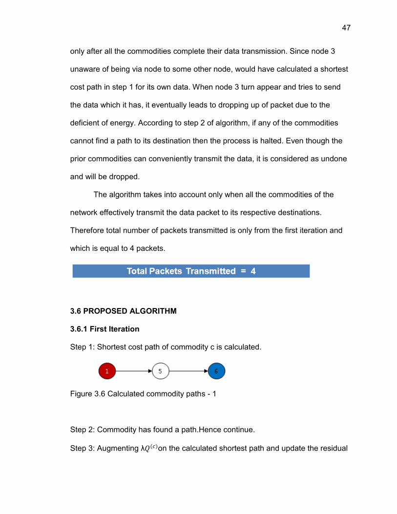
3.6 PROPOSED ALGORITHM
3.6.1 First Iteration
Step 1: Shortest cost path of commodity c is calculated.
Figure 3.6 Calculated commodity paths - 1
Step 2: Commodity has found a path.Hence continue.
Step 3: Augmenting λ on the calculated shortest path and update the residual
48
energy.
Table 3.6 Residual energy update after first iteration (Our Algorithm).
Initial Energy E1 E2 E3 E4 E5 E6 E7 E8
12 12 12 12 12 12 12 12
Residual
Energy
R1 R2 R3 R4 R5 R6 R7 R8
10 12 12 12 9 12 12 12
Step 4: Continue to Step 1.
3.6.2 Second Iteration
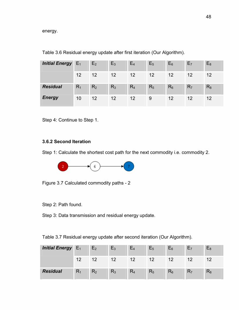
Step 1: Calculate the shortest cost path for the next commodity i.e. commodity 2.
Figure 3.7 Calculated commodity paths - 2
Step 2: Path found.
Step 3: Data transmission and residual energy update.
Table 3.7 Residual energy update after second iteration (Our Algorithm).
Initial Energy E1 E2 E3 E4 E5 E6 E7 E8
12 12 12 12 12 12 12 12
Residual R1 R2 R3 R4 R5 R6 R7 R8
49
Energy 10 8 12 12 9 11 12 12
Step 4: Continue to Step 1.
3.6.3 Third Iteration
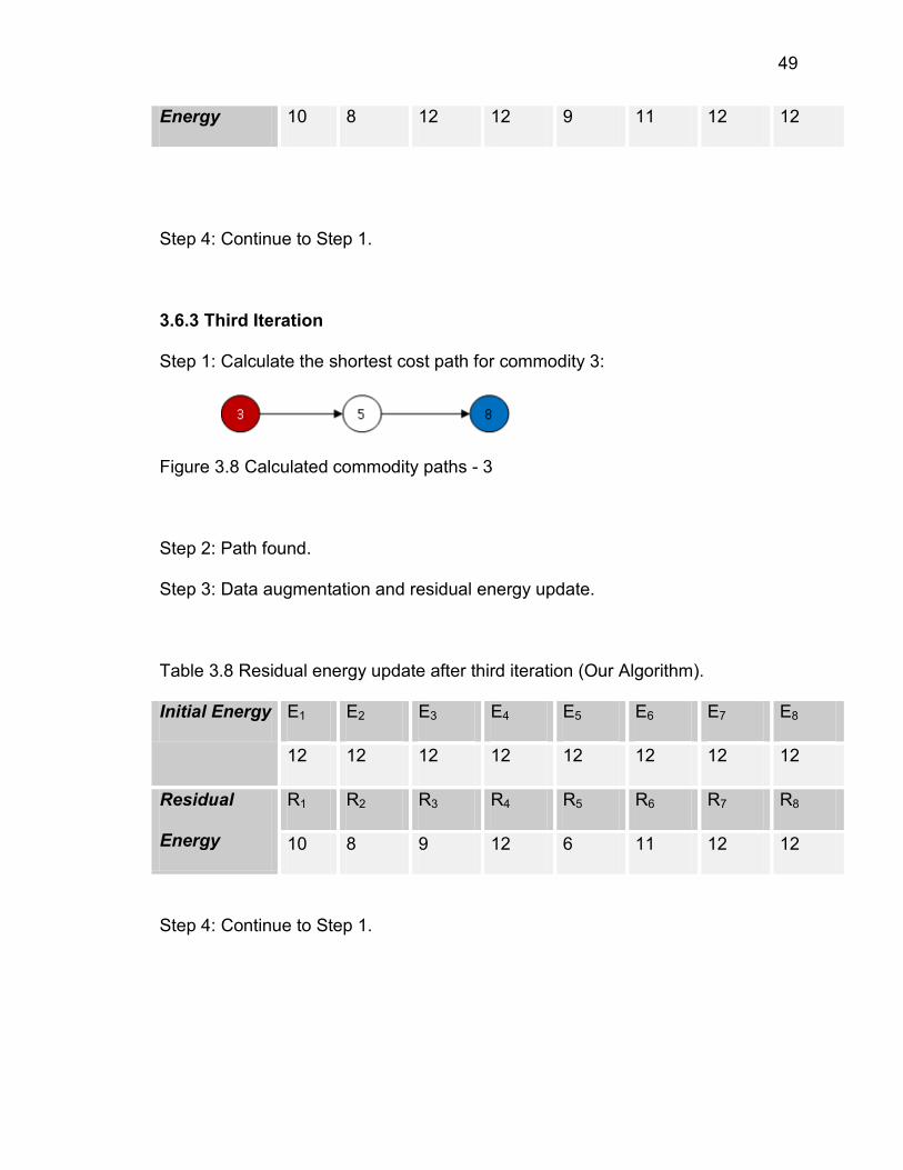
Step 1: Calculate the shortest cost path for commodity 3:
Figure 3.8 Calculated commodity paths - 3
Step 2: Path found.
Step 3: Data augmentation and residual energy update.
Table 3.8 Residual energy update after third iteration (Our Algorithm).
Initial Energy E1 E2 E3 E4 E5 E6 E7 E8
12 12 12 12 12 12 12 12
Residual
Energy
R1 R2 R3 R4 R5 R6 R7 R8
10 8 9 12 6 11 12 12
Step 4: Continue to Step 1.
50
3.6.4 Fourth Iteration
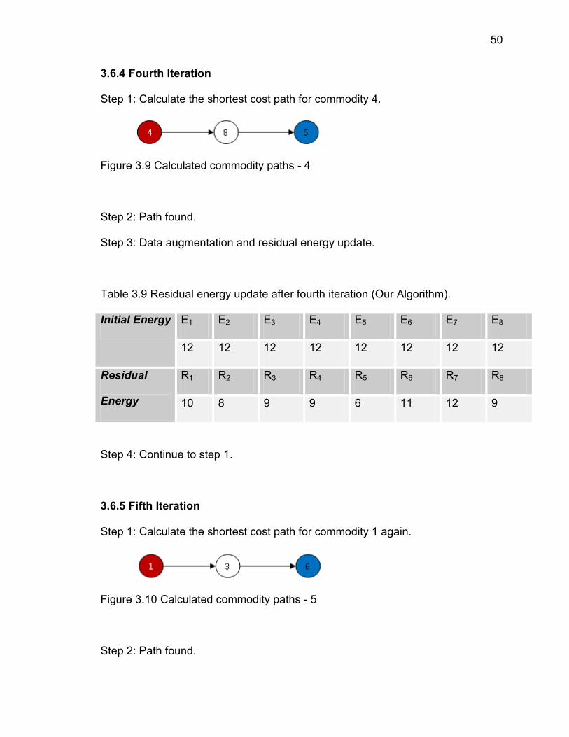
Step 1: Calculate the shortest cost path for commodity 4.
Figure 3.9 Calculated commodity paths - 4
Step 2: Path found.
Step 3: Data augmentation and residual energy update.
Table 3.9 Residual energy update after fourth iteration (Our Algorithm).
Initial Energy E1 E2 E3 E4 E5 E6 E7 E8
12 12 12 12 12 12 12 12
Residual
Energy
R1 R2 R3 R4 R5 R6 R7 R8
10 8 9 9 6 11 12 9
Step 4: Continue to step 1.
3.6.5 Fifth Iteration
Step 1: Calculate the shortest cost path for commodity 1 again.
Figure 3.10 Calculated commodity paths - 5
Step 2: Path found.
51
Step 3: Data augmentation and residual energy update.
Table 3.10 Residual energy update after fifth iteration (Our Algorithm).
Initial Energy E1 E2 E3 E4 E5 E6 E7 E8
12 12 12 12 12 12 12 12
Residual
Energy
R1 R2 R3 R4 R5 R6 R7 R8
9 8 4 9 6 11 12 9
Step 4: Continue to step 1.
3.6.6 Sixth Iteration
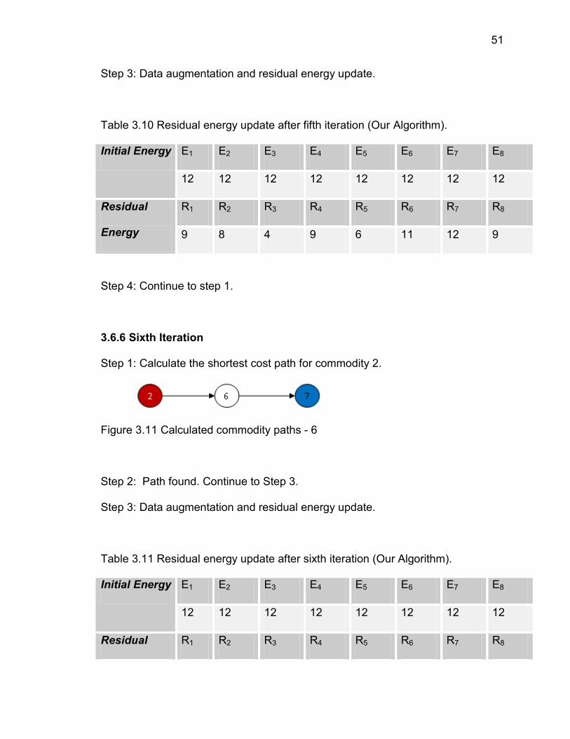
Step 1: Calculate the shortest cost path for commodity 2.
Figure 3.11 Calculated commodity paths - 6
Step 2: Path found. Continue to Step 3.
Step 3: Data augmentation and residual energy update.
Table 3.11 Residual energy update after sixth iteration (Our Algorithm).
Initial Energy E1 E2 E3 E4 E5 E6 E7 E8
12 12 12 12 12 12 12 12
Residual R1 R2 R3 R4 R5 R6 R7 R8
52
Energy 9 4 4 9 6 10 12 9
Step 4: Continue to step 1.
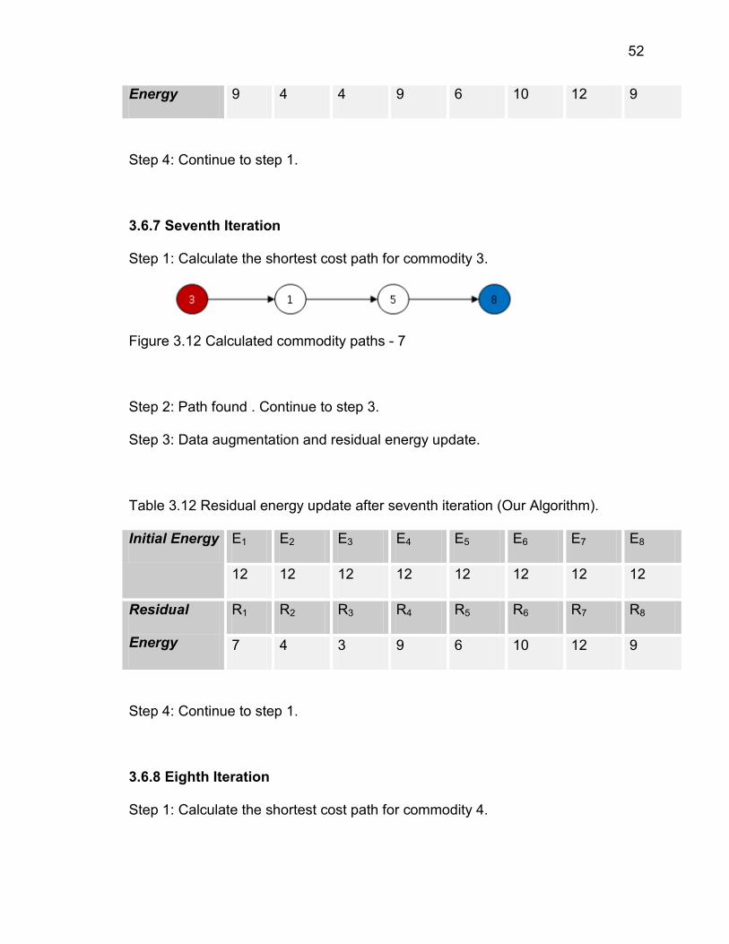
3.6.7 Seventh Iteration
Step 1: Calculate the shortest cost path for commodity 3.
Figure 3.12 Calculated commodity paths - 7
Step 2: Path found . Continue to step 3.
Step 3: Data augmentation and residual energy update.
Table 3.12 Residual energy update after seventh iteration (Our Algorithm).
Initial Energy E1 E2 E3 E4 E5 E6 E7 E8
12 12 12 12 12 12 12 12
Residual
Energy
R1 R2 R3 R4 R5 R6 R7 R8
7 4 3 9 6 10 12 9
Step 4: Continue to step 1.
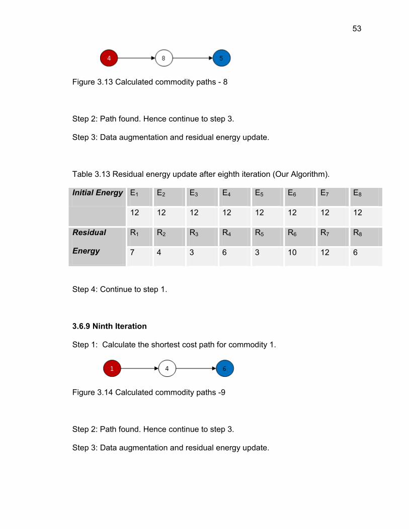
3.6.8 Eighth Iteration
Step 1: Calculate the shortest cost path for commodity 4.
53
Figure 3.13 Calculated commodity paths - 8
Step 2: Path found. Hence continue to step 3.
Step 3: Data augmentation and residual energy update.
Table 3.13 Residual energy update after eighth iteration (Our Algorithm).
Initial Energy E1 E2 E3 E4 E5 E6 E7 E8
12 12 12 12 12 12 12 12
Residual
Energy
R1 R2 R3 R4 R5 R6 R7 R8
7 4 3 6 3 10 12 6
Step 4: Continue to step 1.
3.6.9 Ninth Iteration
Step 1: Calculate the shortest cost path for commodity 1.
Figure 3.14 Calculated commodity paths -9
Step 2: Path found. Hence continue to step 3.
Step 3: Data augmentation and residual energy update.

54
Table 3.14 Residual energy update after ninth iteration (Our Algorithm).
Initial Energy E1 E2 E3 E4 E5 E6 E7 E8
12 12 12 12 12 12 12 12
Residual
Energy
R1 R2 R3 R4 R5 R6 R7 R8
2 4 3 2 3 10 12 6
Step 4: Continue to step 1.
3.6.10 Tenth Iteration
Step 1: Calculate the shortest cost path for commodity 2.
Path could not be found for commodity 2 due to the inadequate energy.
Figure 3.15 Calculated commodity paths - 10
Step 2: Path not found. Hence stop.
Therefore total number of packets transmitted is all the packets delivered
from first iteration through ninth iteration, which is equal to 9 packets.
3.7 KEY FEATURE
A difference of 5 packets is a big accomplishment for this small network. If

55
we look at the residual energy table at the end of the simulation, it is very clear
that nodes are more widely spread in our algorithm compared to the flow
augmentation algorithm, excelling in prolonging the system lifetime.
The serious drawback of FA algorithm is updating the residual energy, which
takes place after all the commodities complete their productive data transmission
i.e. at the end of the iteration. By doing this, it encourages nodes to assume
energy falsely and try to communicate with other nodes, which ultimately
accompany in depletion of data.
Unlike in FA algorithm, our algorithm routes the packets through paths that
may be longer but that pass through nodes that have excess of energy resource,
leading to maximize the node lifetime. Importantly there is a zero probability of
node being placed in false assumption of energy thus avoiding the packet drop.
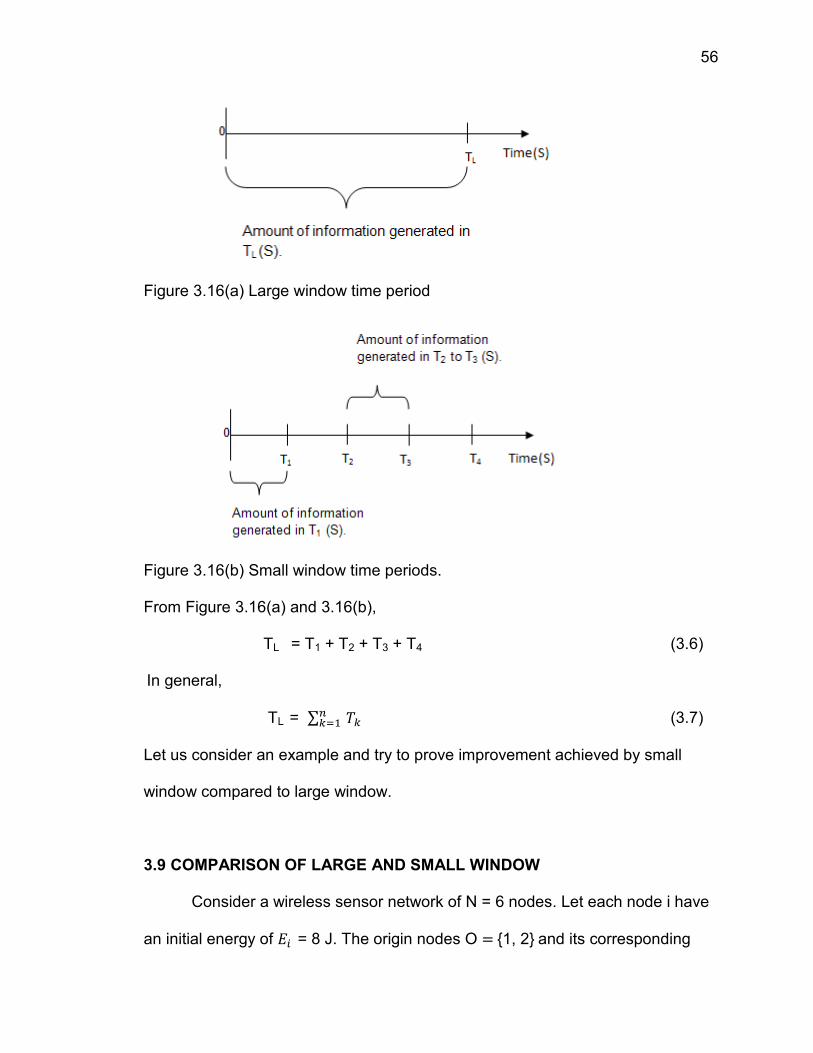
3.8 COMPETENCE OF SMALLER WINDOW AGAINST LARGE WINDOW
Here the lifetime achieved for large window is compared with lifetime of
the small window, where a large window is defined as the amount of information
generated for a time period of TL seconds and small window is defined as the
amount of information generated at each sub-divided intervals of TL seconds.
Figure 3.16(a) and (b) shows the pictorial representation of large window and
small window respectively.
56
Figure 3.16(a) Large window time period
Figure 3.16(b) Small window time periods.
From Figure 3.16(a) and 3.16(b),
TL = T1 + T2 + T3 + T4 (3.6)
In general,
TL = (3.7)
Let us consider an example and try to prove improvement achieved by small
window compared to large window.
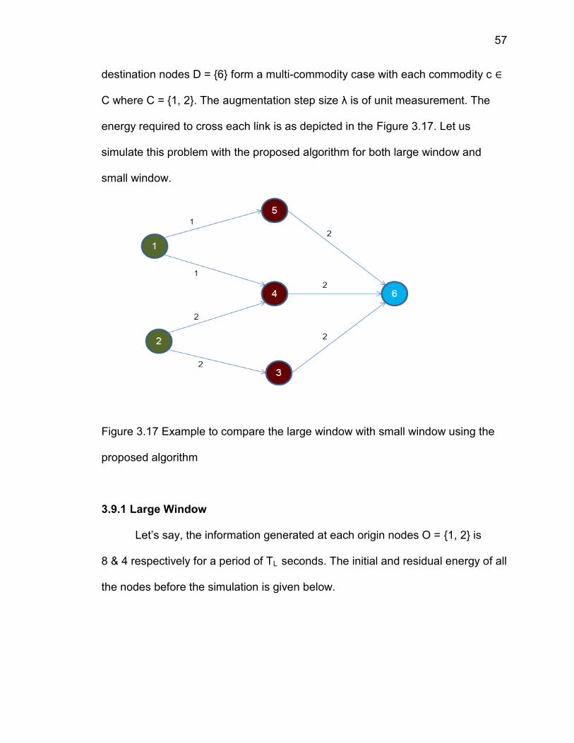
3.9 COMPARISON OF LARGE AND SMALL WINDOW
Consider a wireless sensor network of N = 6 nodes. Let each node i have
an initial energy of = 8 J. The origin nodes O = {1, 2} and its corresponding
57
destination nodes D = {6} form a multi-commodity case with each commodity c ∈
C where C = {1, 2}. The augmentation step size λ is of unit measurement. The
energy required to cross each link is as depicted in the Figure 3.17. Let us
simulate this problem with the proposed algorithm for both large window and
small window.
Figure 3.17 Example to compare the large window with small window using the
proposed algorithm
3.9.1 Large Window
Let’s say, the information generated at each origin nodes O = {1, 2} is
8 & 4 respectively for a period of TL seconds. The initial and residual energy of all
the nodes before the simulation is given below.
58
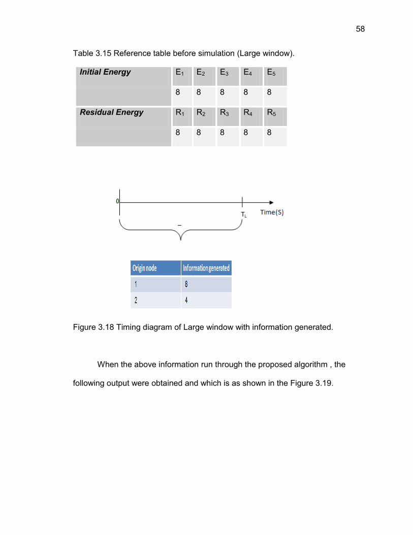
Table 3.15 Reference table before simulation (Large window).
Initial Energy E1 E2 E3 E4 E5
8 8 8 8 8
Residual Energy R1 R2 R3 R4 R5
8 8 8 8 8
Figure 3.18 Timing diagram of Large window with information generated.
When the above information run through the proposed algorithm , the
following output were obtained and which is as shown in the Figure 3.19.
59
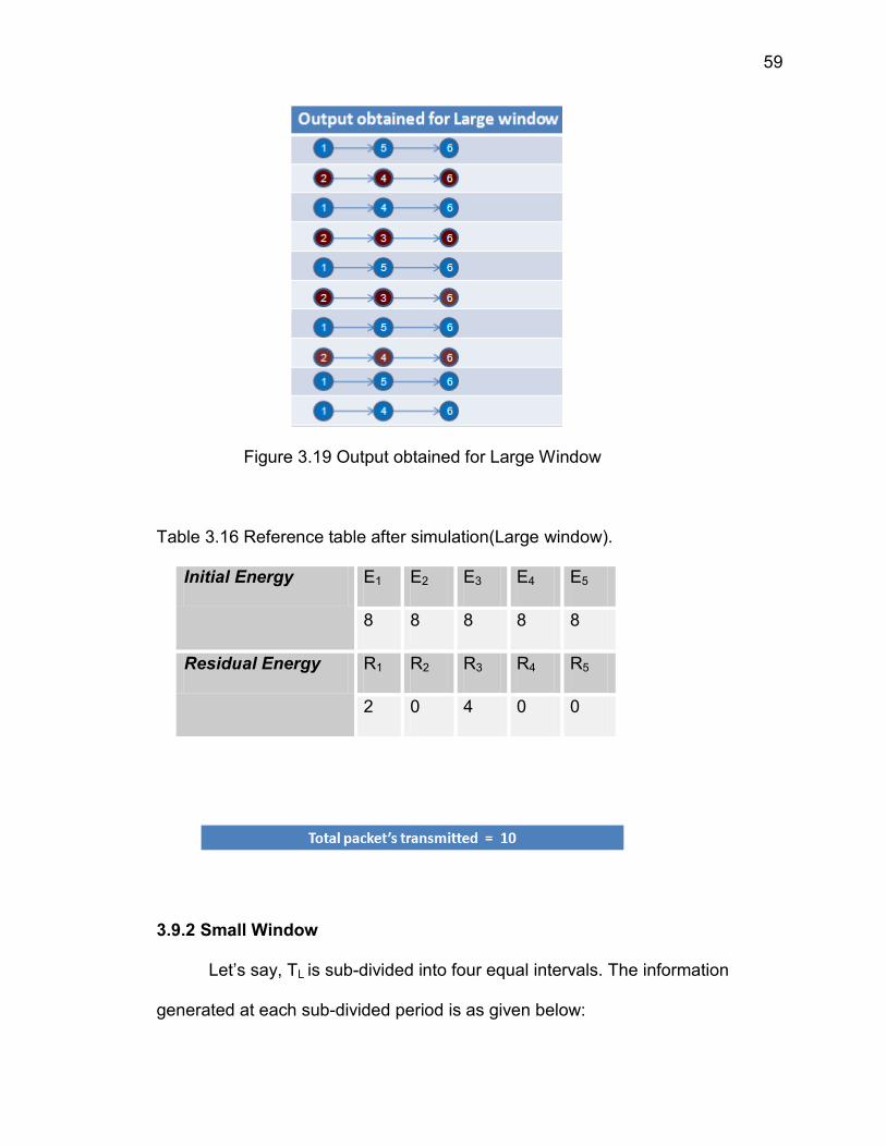
Figure 3.19 Output obtained for Large Window
Table 3.16 Reference table after simulation(Large window).
Initial Energy E1 E2 E3 E4 E5
8 8 8 8 8
Residual Energy R1 R2 R3 R4 R5
2 0 4 0 0
3.9.2 Small Window
Let’s say, TL is sub-divided into four equal intervals. The information
generated at each sub-divided period is as given below:
60
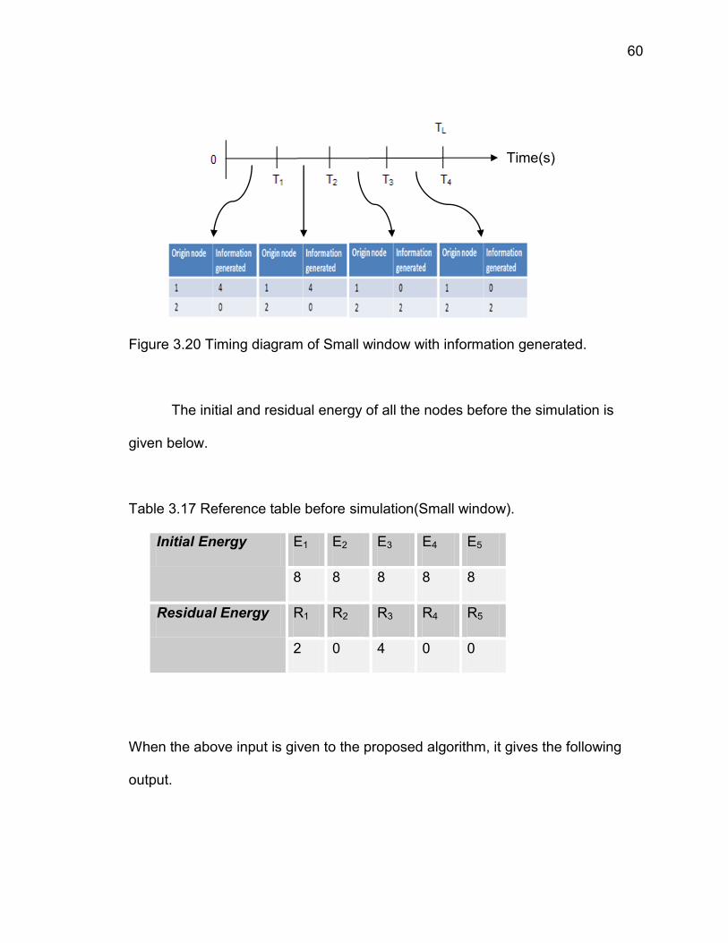
Figure 3.20 Timing diagram of Small window with information generated.
The initial and residual energy of all the nodes before the simulation is
given below.
Table 3.17 Reference table before simulation(Small window).
Initial Energy E1 E2 E3 E4 E5
8 8 8 8 8
Residual Energy R1 R2 R3 R4 R5
2 0 4 0 0
When the above input is given to the proposed algorithm, it gives the following
output.
Time(s)
61
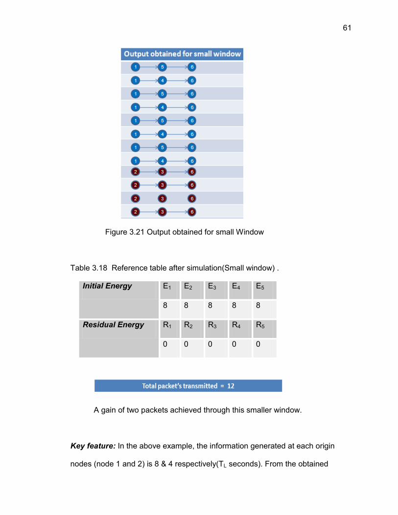
Figure 3.21 Output obtained for small Window
Table 3.18 Reference table after simulation(Small window) .
Initial Energy E1 E2 E3 E4 E5
8 8 8 8 8
Residual Energy R1 R2 R3 R4 R5
0 0 0 0 0
A gain of two packets achieved through this smaller window.
Key feature: In the above example, the information generated at each origin
nodes (node 1 and 2) is 8 & 4 respectively(TL seconds). From the obtained
62
result, it demonstrates that there is a scarce for two packets of source 1 with
large window as compared to the small window. The reason behind this is,
source 2 utilizing the allocated resource of source 1 to transmit two of its data
packet to its destination node (node 6). In doing this, source 2 made source 1
deficient of two packets.
In small window, the time period is sub-divided into 4 equal intervals
TL = T1 + T2 + T3 + T4 (3.8)
It is not the case in large window, where information generated is
encountered at one shot which is after TL seconds. At T1, the information
generated at each origin nodes (node 1 and node 2) is 4 and 0 respectively. Now
source 1 transmits the received packets to its destination node (node 6). At T2,
the information generated is again 4 and 0 at respected nodes (node 1 and node
2). Source 1 relays the received packet to its corresponding destination. Hence,
till T2 there is no botheration from source 2 on allocated resource of source 1,
which made source 1 in successful transmission . At T3, the information
generated at origin nodes (node 1 and node 2) are 0 and 2 respectively. And also
at T4, same amount of information is generated. Now source 2 transmits all of its
received packets efficiently to its destination node (node 6) out of its solely
allocated resource, leading to achieve the optimal solution of 12 packets.

63
CHAPTER 4
RESULTS AND CONCLUSION
In this section, we evaluate the performance of our heuristic and compare
it to that proposed in [21]. In section 3.5, we saw how it is possible to maximize
the system lifetime. In this section, we provide graphical results to support the
conclusion made in section 3.5.
4.1 RESULTS TO SHOW INCREASE IN LIFETIME:
We use a static network of sensors for simulation purposes. The
adjustable parameters are:
N the number of sensor nodes. We vary this from 5 to 300.
B the battery level of sensor nodes.
By varying the number of commodities with fixed number of nodes and
fixed battery level.
By varying the load for fixed number of nodes N, fixed battery level
and fixed commodity c.
In order to compare our results with [21], we use the constant information
generation rates model defined by them. Let SX denote the ratio between the
system lifetime obtained by algorithm X and the optimal solution and be called
the normalized network lifetime.

64
We will also evaluate the percentage gain of proposed algorithm to that of
flow augmentation algorithm with following formulation.
=
We have implemented our algorithm in C++ and run experiments on randomly
generated graphs. For performance comparison, the optimal solution is obtained
from the lp solver after solving the linear programming problem. Note that λ is of
unit measurement.
4.2 RESULTS FOR VARYING NUMBER OF NODES
The comparison in terms of normalized lifetime is made in Table 4.2 and
depicted in Figure 4.2. In table 4.2, the terms SPA denotes the normalized lifetime
of proposed algorithm, SFA denotes normalized lifetime of flow augmentation
algorithm and is the percentage gain of proposed algorithm over FA
algorithm.
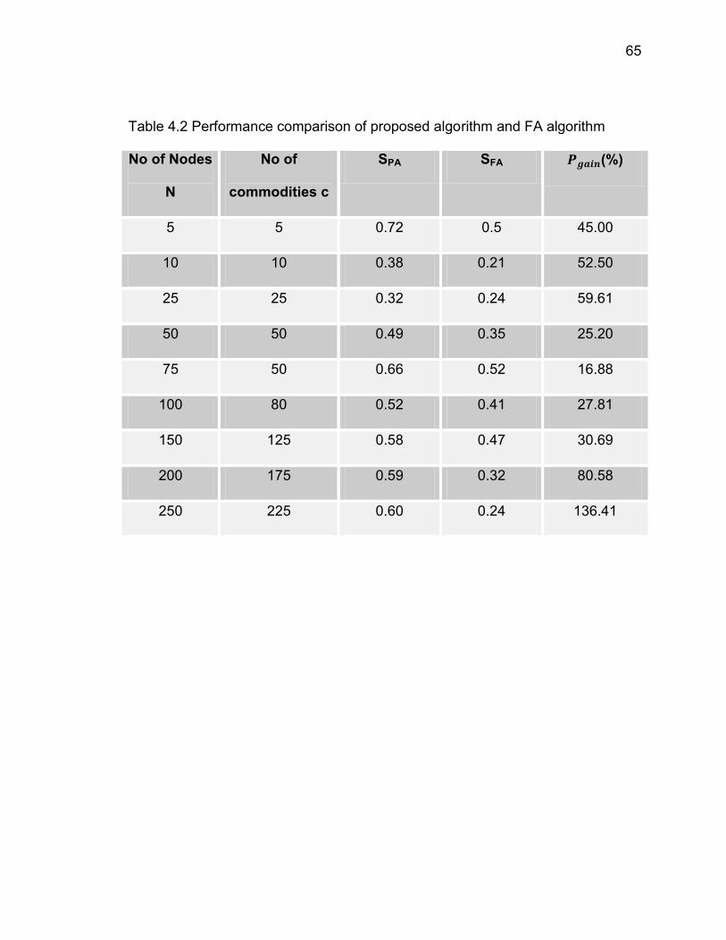
65
Table 4.2 Performance comparison of proposed algorithm and FA algorithm
No of Nodes
N
No of
commodities c
SPA SFA (%)
5 5 0.72 0.5 45.00
10 10 0.38 0.21 52.50
25 25 0.32 0.24 59.61
50 50 0.49 0.35 25.20
75 50 0.66 0.52 16.88
100 80 0.52 0.41 27.81
150 125 0.58 0.47 30.69
200 175 0.59 0.32 80.58
250 225 0.60 0.24 136.41
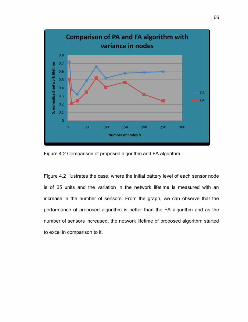
66
Figure 4.2 Comparison of proposed algorithm and FA algorithm
Figure 4.2 illustrates the case, where the initial battery level of each sensor node
is of 25 units and the variation in the network lifetime is measured with an
increase in the number of sensors. From the graph, we can observe that the
performance of proposed algorithm is better than the FA algorithm and as the
number of sensors increased, the network lifetime of proposed algorithm started
to excel in comparison to it.
0
0.1
0.2
0.3
0.4
0.5
0.6
0.7
0.8
0 50 100 150 200 250 300
S, n
orm
aliz
ed
ne
two
rk li
feti
me
Number of nodes N
Comparison of PA and FA algorithm with variance in nodes
PA
FA
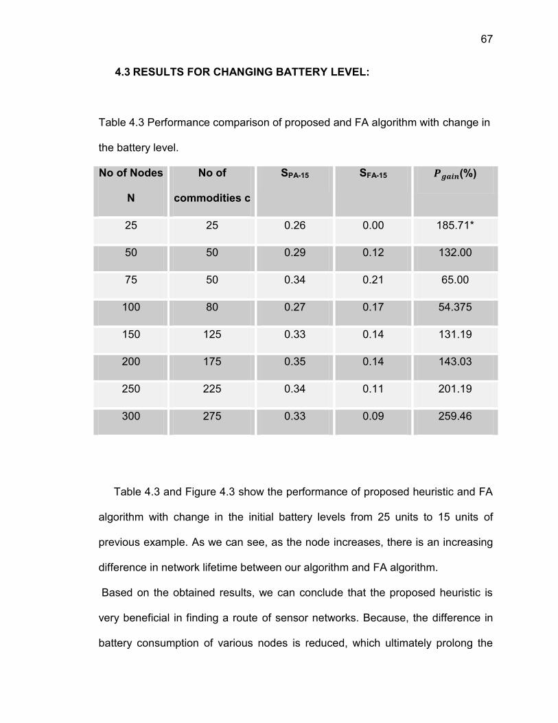
67
4.3 RESULTS FOR CHANGING BATTERY LEVEL:
Table 4.3 Performance comparison of proposed and FA algorithm with change in
the battery level.
No of Nodes
N
No of
commodities c
SPA-15 SFA-15 (%)
25 25 0.26 0.00 185.71*
50 50 0.29 0.12 132.00
75 50 0.34 0.21 65.00
100 80 0.27 0.17 54.375
150 125 0.33 0.14 131.19
200 175 0.35 0.14 143.03
250 225 0.34 0.11 201.19
300 275 0.33 0.09 259.46
Table 4.3 and Figure 4.3 show the performance of proposed heuristic and FA
algorithm with change in the initial battery levels from 25 units to 15 units of
previous example. As we can see, as the node increases, there is an increasing
difference in network lifetime between our algorithm and FA algorithm.
Based on the obtained results, we can conclude that the proposed heuristic is
very beneficial in finding a route of sensor networks. Because, the difference in
battery consumption of various nodes is reduced, which ultimately prolong the
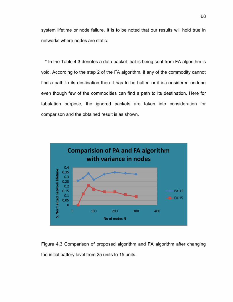
68
system lifetime or node failure. It is to be noted that our results will hold true in
networks where nodes are static.
* In the Table 4.3 denotes a data packet that is being sent from FA algorithm is
void. According to the step 2 of the FA algorithm, if any of the commodity cannot
find a path to its destination then it has to be halted or it is considered undone
even though few of the commodities can find a path to its destination. Here for
tabulation purpose, the ignored packets are taken into consideration for
comparison and the obtained result is as shown.
Figure 4.3 Comparison of proposed algorithm and FA algorithm after changing
the initial battery level from 25 units to 15 units.
00.050.1
0.150.2
0.250.3
0.350.4
0 100 200 300 400
S, N
orm
aliz
ed
ne
two
rk li
feti
me
No of nodes N
Comparision of PA and FA algorithm with variance in nodes
PA-15
FA-15
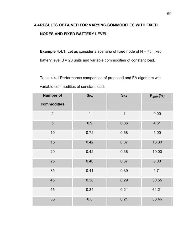
69
4.4 RESULTS OBTAINED FOR VARYING COMMODITIES WITH FIXED
NODES AND FIXED BATTERY LEVEL:
Example 4.4.1: Let us consider a scenario of fixed node of N = 75, fixed
battery level B = 20 units and variable commodities of constant load.
Table 4.4.1 Performance comparison of proposed and FA algorithm with
variable commodities of constant load.
Number of
commodities
SPA SFA (%)
2 1 1 0.00
5 0.9 0.86 4.61
10 0.72 0.68 5.00
15 0.42 0.37 13.33
20 0.42 0.38 10.00
25 0.40 0.37 8.00
35 0.41 0.39 5.71
45 0.38 0.29 30.55
55 0.34 0.21 61.21
65 0.3 0.21 38.46
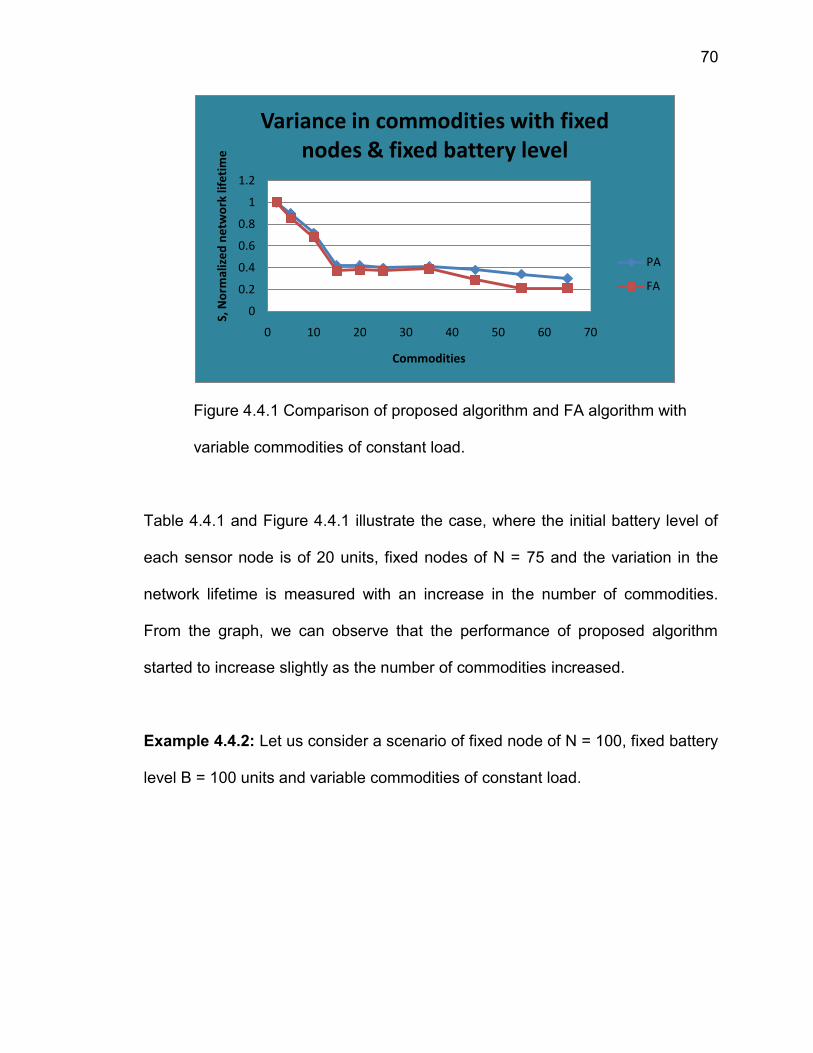
70
Figure 4.4.1 Comparison of proposed algorithm and FA algorithm with
variable commodities of constant load.
Table 4.4.1 and Figure 4.4.1 illustrate the case, where the initial battery level of
each sensor node is of 20 units, fixed nodes of N = 75 and the variation in the
network lifetime is measured with an increase in the number of commodities.
From the graph, we can observe that the performance of proposed algorithm
started to increase slightly as the number of commodities increased.
Example 4.4.2: Let us consider a scenario of fixed node of N = 100, fixed battery
level B = 100 units and variable commodities of constant load.
0
0.2
0.4
0.6
0.8
1
1.2
0 10 20 30 40 50 60 70
S, N
orm
aliz
ed
ne
two
rk li
feti
me
Commodities
Variance in commodities with fixed nodes & fixed battery level
PA
FA
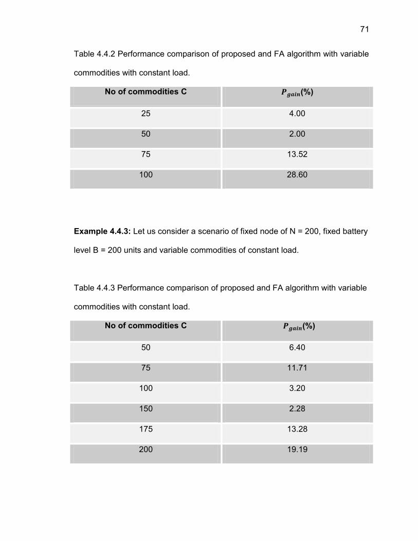
71
Table 4.4.2 Performance comparison of proposed and FA algorithm with variable
commodities with constant load.
No of commodities C (%)
25 4.00
50 2.00
75 13.52
100 28.60
Example 4.4.3: Let us consider a scenario of fixed node of N = 200, fixed battery
level B = 200 units and variable commodities of constant load.
Table 4.4.3 Performance comparison of proposed and FA algorithm with variable
commodities with constant load.
No of commodities C (%)
50 6.40
75 11.71
100 3.20
150 2.28
175 13.28
200 19.19

72
Table 4.4.2 and Table 4.4.3 show the percentage gain of proposed
algorithm over flow augmentation algorithm with varying commodities of constant
load. Here in this table, the normalized network lifetime or is not shown,
as the optimal solution could not be obtained for commodities due to the
increasing number of unknown variables.
From the table, one can say that as the number of commodities starts increasing
with fixed number of nodes and battery level, the performance of our algorithm
outperforms FA algorithm.
4.5 RESULTS OBTAINED FOR VARYING LOADS WITH FIXED NODES,
FIXED BATTERY LEVEL AND FIXED COMMODITY:
Now let us consider a scenario of fixed nodes, fixed battery level and fixed
commodity. But vary the load of data that needs to be transmitted out of
commodity c.
Example 4.5.1: Let us consider a fixed node of N = 75, fixed battery level B =
100 units and fixed commodity C = 35.
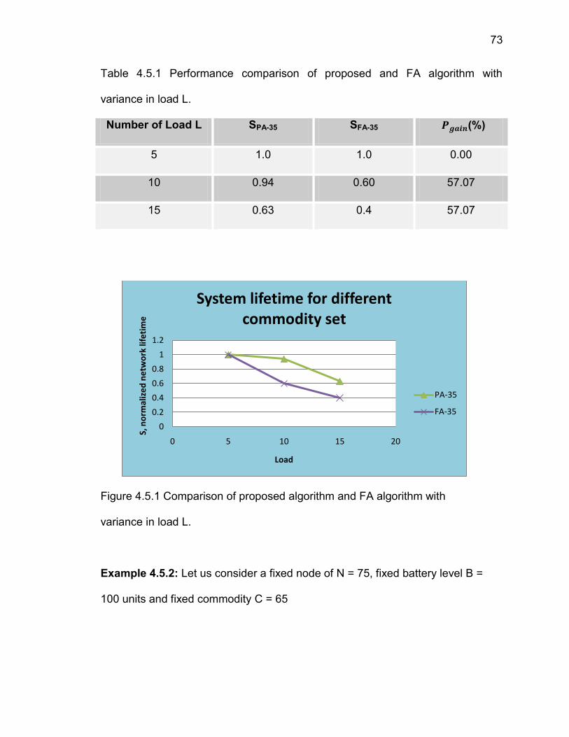
73
Table 4.5.1 Performance comparison of proposed and FA algorithm with
variance in load L.
Number of Load L SPA-35 SFA-35 (%)
5 1.0 1.0 0.00
10 0.94 0.60 57.07
15 0.63 0.4 57.07
Figure 4.5.1 Comparison of proposed algorithm and FA algorithm with
variance in load L.
Example 4.5.2: Let us consider a fixed node of N = 75, fixed battery level B =
100 units and fixed commodity C = 65
0
0.2
0.4
0.6
0.8
1
1.2
0 5 10 15 20
S, n
orm
aliz
ed
ne
two
rk li
feti
me
Load
System lifetime for different commodity set
PA-35
FA-35
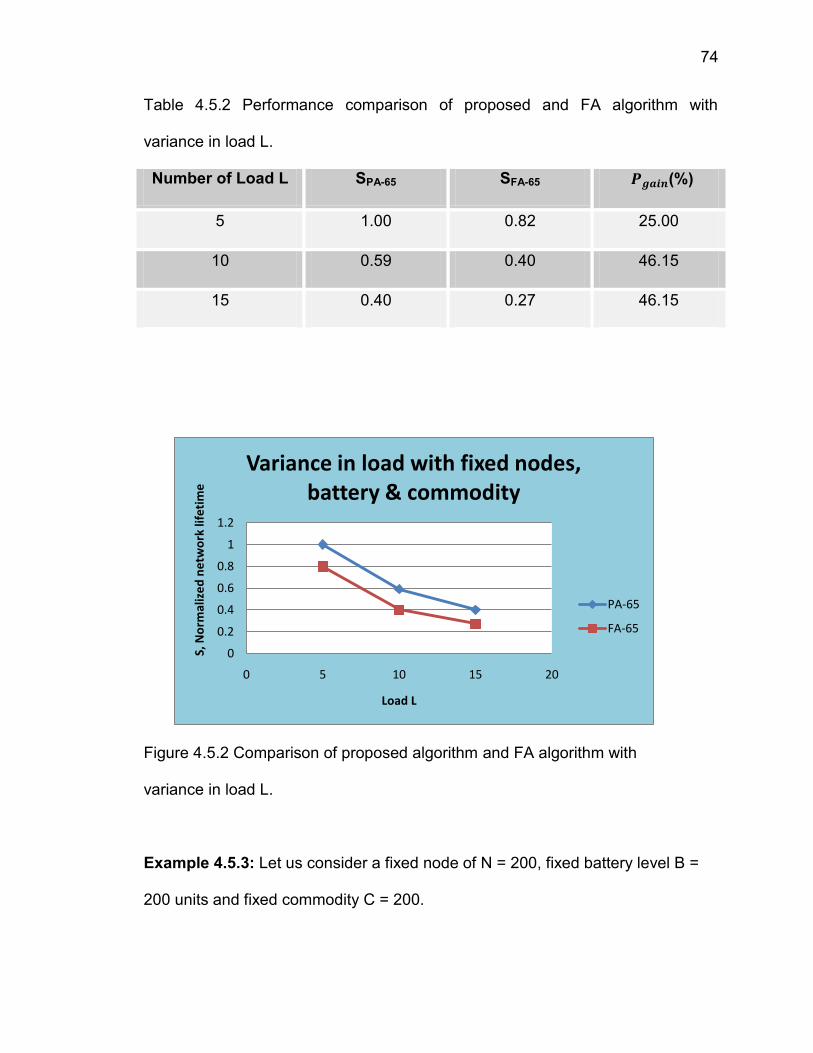
74
Table 4.5.2 Performance comparison of proposed and FA algorithm with
variance in load L.
Number of Load L SPA-65 SFA-65 (%)
5 1.00 0.82 25.00
10 0.59 0.40 46.15
15 0.40 0.27 46.15
Figure 4.5.2 Comparison of proposed algorithm and FA algorithm with
variance in load L.
Example 4.5.3: Let us consider a fixed node of N = 200, fixed battery level B =
200 units and fixed commodity C = 200.
0
0.2
0.4
0.6
0.8
1
1.2
0 5 10 15 20
S, N
orm
aliz
ed
ne
two
rk li
feti
me
Load L
Variance in load with fixed nodes, battery & commodity
PA-65
FA-65
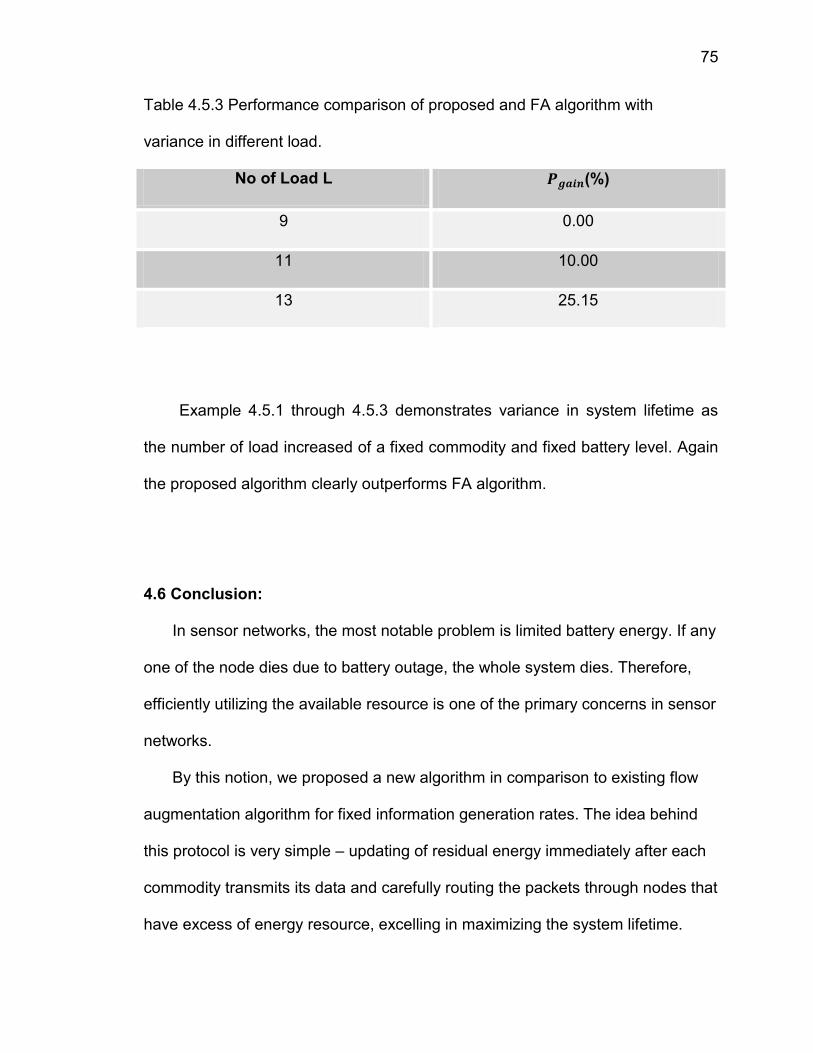
75
Table 4.5.3 Performance comparison of proposed and FA algorithm with
variance in different load.
No of Load L (%)
9 0.00
11 10.00
13 25.15
Example 4.5.1 through 4.5.3 demonstrates variance in system lifetime as
the number of load increased of a fixed commodity and fixed battery level. Again
the proposed algorithm clearly outperforms FA algorithm.
4.6 Conclusion:
In sensor networks, the most notable problem is limited battery energy. If any
one of the node dies due to battery outage, the whole system dies. Therefore,
efficiently utilizing the available resource is one of the primary concerns in sensor
networks.
By this notion, we proposed a new algorithm in comparison to existing flow
augmentation algorithm for fixed information generation rates. The idea behind
this protocol is very simple – updating of residual energy immediately after each
commodity transmits its data and carefully routing the packets through nodes that
have excess of energy resource, excelling in maximizing the system lifetime.
76
More importantly there is no conflict between commodities as in FA algorithm,
sharing a common resource for different data packets leading to data collapse.
The simulation results showed that the proposed heuristic performance is always
better than the flow augmentation algorithm. This is a significant theoretical
improvement over the previously proposed FA heuristics. Also analyzed the
significance of smaller information generation window against larger information
generation window and showed the importance of smaller window.
77
REFERENCES
[1] F.L. Lewis, “Wireless Sensor Networks, To appear smart environments:
Technologies, Protocols and Applications”, ed. D.J.Cook and S.K.Das, John
Wiley, NewYork, 2004.
[2] Wikipedia - http://en.wikipedia.org/wiki/Wireless_sensor_network
[3] Yang Yu (Motorola Labs, USA), Viktor K Prasanna (University of Southern
California, USA), & Bhaskar Krishnamachari (University of Southern
California, USA), “INFORMATION PROCESSING AND ROUTING IN
WIRELESS SENSOR NETWORKS”, ISBN: 978-981-277-258-9.
[4] Courtesy of Artech House, R. Frank 2000.
[5] Jorge Tavares, Fernando J. Velez, João M. Ferro, “ Application of Wireless
Sensor Networks to Automobiles,“ MEASUREMENT SCIENCE REVIEW,
Volume 8, Section 3, No. 3, 2008.
[6] Dr.Rajender Thusu, PhD, Frost & Sullivan, “Wireless Sensor Use is
Expanding in Industrial Applications,” Sensor Magzine, June 1, 2010.
[7] John A. Stankovic, “Research Challenges for Wireless Sensor Networks,”
ACM New York, NY, USA, vol 1, issue 2, July 2004.
[8] Yong Yuan*, Zongkai Yang, Min Chen and Jianhua He, “A survey on
information processing technologies in wireless sensor networks,“ Int. J. Ad
Hoc and Ubiquitous Computing, Vol. x, No. x, 200x.
[9] Chris Townsend, Steven Arms, “Wireless Sensor Networks: Principles and
Applications,” WilsonChapter22.indd.
78
[10] Chunkai Yin and Ali Orooji, “Routing Protocols for Sensor Networks,”
CiteSeerX.
[11] Imad Mahgoub and Mohammad Ilyas, “Sensor Network Protocols,” CRC
press, pp. 9-4, 2005.
[12] Kemal Akkaya and Mohamed Younis, “A Survey of Routing Protocols in
Wireless Sensor Networks,” in the Elsevier Ad Hoc Network Journal, Vol 3/3
pp. 325-349, 2005.
[13] Heinzelman, W. R., Kulic, J., Balakrishnan, H., “Adaptive Protocol for
Information Dissemination in Wireless Sensor Networks,” Fifth ACM/IEEE
MOBICOM, Conference, Seattle, WA, 1999.
[14] Intanagonwiwat, C., Ramesh, Govindan, R., Estrin, D., Heidemann, J.,
and Silva, F., “Directed Diffusion for Wireless Sensor Networking Pages 2-16,
IEEE/ACM Transactions on networking, vol. 11, no. 1, February 2003.
[15] Archana Bharathidasan, Vijay Anand Sai Ponduru, “Sensor Networks: An
Overview”, Department of Computer Science, University of California, Davis,
CA 95616.
[16] Heinzelman, W.R., Chandrakasan, A., and Balakrishnan, H., “Energy-
Efficient Communication Protocol for Wireless Micro-sensor Networks,”
Proceedings of the Hawaii International Conference on System Sciences,
January 4-7, 2000, Maui, Hawaii (IEEE).
[17] Dr. Dheeraj Sanghi and Nilesh Mishra, “Routing in Wireless Sensor
Networks,” CiteSeerX.
79
[18] A. Manjeshwar and D. P. Agrawal, “TEEN: A Protocol for Enhanced
Efficiency in Wireless Sensor Networks,” Proceedings of the 1st International
Workshop on Parallel and Distributed Computing Issues in Wireless Networks
and Mobile Computing, San Francisco, CA, April 2001.
[19] Y. Xu, J. Heidemann, D. Estrin, “Geography-informed Energy
Conservation for Ad-hoc Routing,” In Proceedings of the Seventh Annual
ACM/IEEE International Conference on Mobile Computing and Networking
2001, pp. 70-84.
[20] Y. Yu, D. Estrin, and R. Govindan, “Geographical and Energy-Aware
Routing: A Recursive Data Dissemination Protocol for Wireless Sensor
Networks,” UCLA Computer Science Department Technical Report, UCLA-
CSD TR-01-0023, May 2001.
[21] Jae-Hwan Chang, Leandros Tassiulas, “Maximum lifetime routing in
wireless sensor networks,” IEEE/ACM Transactions on Networking (TON),
Volume 12 Issue 4, August 2004.
[22] S. G. Nash and A. Sofer, “Linear and Nonlinear Programming,” New
York: McGraw-Hill, 1996.
[23] S. Singh, M.Woo, and C. S. Raghavendra, “Power-aware routing in mobile
ad-hoc networks,” in Proc. 4th Annu. IEEE/ACM Int. Conf. Mobile Computing
and Networking, Dallas, TX, Oct. 1998, pp. 181–190.
[24] http://www.opalsoft.net/qos/Q-OSPF-50.htm

80
VITA
Graduate School
Southern Illinois University
Karthik Kuppaswamy
Email: [email protected]
Visvesvaraya Technological University, Bangalore.
Bachelor of Engineering, Electronics & Communication, May 2007
Theses Title:
Maximizing the System Lifetime in Wireless Sensor Networks using
Improved Routing Algorithm
Major Professor: Dimitrios Kagaris