Maxima by Example: Ch.9: Bigfloats and High Accuracy Quadrature
40
Maxima by Example: Ch.9: Bigfloats and High Accuracy Quadrature ∗ Edwin L. (Ted) Woollett May 30, 2016 Contents 1 Introduction 3 2 Bigfloat Numbers in Maxima 3 2.1 Experimenting with Bigfloats ................................... 4 2.2 Bigfloat Numbers and fpprintprec ............................... 8 2.3 Using print with Bigfloats .................................... 12 2.4 Using printf with Bigfloats .................................... 13 2.5 A Table of Bigfloats using printf ................................ 13 2.6 Adding Bigfloats Having Differing Accuracy .......................... 14 2.7 Polynomial Roots Using bfallroots ................................ 15 2.8 Finding Highly Accurate Roots using bf find root ........................ 19 2.9 Bigfloat Number Gaps and Binary Arithmetic .......................... 20 2.10 Effect of Floating Point Precision on Function Evaluation .................... 23 3 High Accuracy Quadrature with Maxima 24 3.1 Using bromberg for High Accuracy Quadrature ........................ 24 3.2 A Double Exponential Quadrature Method for a ≤ x < ∞ .................. 28 3.3 The tanh-sinh Quadrature Method for a ≤ x ≤ b ........................ 31 3.4 The Gauss-Legendre Quadrature Method for a ≤ x ≤ b ................... 37 * This version uses Maxima 5.36.1 SBCL. This is a live document. Check http://web.csulb.edu/ ˜ woollett/ for the latest version of these notes. Send comments and suggestions to [email protected] 1
Transcript of Maxima by Example: Ch.9: Bigfloats and High Accuracy Quadrature

Maxima by Example:Ch.9: Bigfloats and High Accuracy Quadrature∗
Edwin L. (Ted) Woollett
May 30, 2016
Contents
1 Introduction 3
2 Bigfloat Numbers in Maxima 32.1 Experimenting with Bigfloats . . . . . . . . . . . . . . . . . . . . . . .. . . . . . . . . . . . 42.2 Bigfloat Numbers andfpprintprec . . . . . . . . . . . . . . . . . . . . . . . . . . . . . . . 82.3 Usingprint with Bigfloats . . . . . . . . . . . . . . . . . . . . . . . . . . . . . . . . . . . . 122.4 Usingprintf with Bigfloats . . . . . . . . . . . . . . . . . . . . . . . . . . . . . . . . . . . . 132.5 A Table of Bigfloats usingprintf . . . . . . . . . . . . . . . . . . . . . . . . . . . . . . . . 132.6 Adding Bigfloats Having Differing Accuracy . . . . . . . . . . .. . . . . . . . . . . . . . . 142.7 Polynomial Roots Usingbfallroots . . . . . . . . . . . . . . . . . . . . . . . . . . . . . . . . 152.8 Finding Highly Accurate Roots using bffind root . . . . . . . . . . . . . . . . . . . . . . . . 192.9 Bigfloat Number Gaps and Binary Arithmetic . . . . . . . . . . . .. . . . . . . . . . . . . . 202.10 Effect of Floating Point Precision on Function Evaluation . . . . . . . . . . . . . . . . . . . . 23
3 High Accuracy Quadrature with Maxima 243.1 Usingbromberg for High Accuracy Quadrature . . . . . . . . . . . . . . . . . . . . . . . . 243.2 A Double ExponentialQuadrature Method fora ≤ x < ∞ . . . . . . . . . . . . . . . . . . 283.3 Thetanh-sinh Quadrature Method fora ≤ x ≤ b . . . . . . . . . . . . . . . . . . . . . . . . 313.4 TheGauss-LegendreQuadrature Method fora ≤ x ≤ b . . . . . . . . . . . . . . . . . . . 37
∗This version usesMaxima 5.36.1 SBCL. This is a live document. Checkhttp://web.csulb.edu/ ˜ woollett/ forthe latest version of these notes. Send comments and suggestions [email protected]
1

Preface
COPYING AND DISTRIBUTION POLICYThis document is part of the series Maxima by Example, and is m ade availablevia the author’s webpage http://www.csulb.edu/˜woollett /to aid new users of the Maxima computer algebra system.
NON-PROFIT PRINTING AND DISTRIBUTION IS PERMITTED.
You may make copies of this document and distribute themto others as long as you charge no more than the costs of printi ng.
Feedback from readers is the best way for this series of notesto become more helpful to new users of Maxima.All comments and suggestions for improvements will be appreciated and carefully considered.
LOADING FILESThe defaults allow you to use the brief version load(brmbrg) to load in theMaxima file brmbrg.lisp (for example).To load in your own file, such as bfloat.mac (used in this chap ter),using the brief version load(bfloat), you either need to pla cebfloat.mac in one of the folders Maxima searches by default, orelse put a line like (this assumes your work folder is c:\work 3):
file_search_maxima : append(["c:/work3/###.{mac,mc}"] ,file_search_maxima )$
in your personal startup file maxima-init.mac (see Ch. 1, In troduction to Maximafor more information about this).
Otherwise you need to provide a complete path in double quote s,as in load("c:/work3/bfloat.mac"),
We always use the brief load version in our examples, which ar e generatedusing the Xmaxima graphics interface on a computer using the Windowsoperating system. Our maxima-init.mac file also contains d isplay2d:false$,which allows more information per XMaxima screen, and also a llows one tocopy output and directly use it in a further step.
Maxima, a Computer Algebra System.Some numerical results depend on the Lisp version used.This chapter uses Version 5.36.1 ( SBCL).http://maxima.sourceforge.net/
2
1 INTRODUCTION 3
1 Introduction
This chapter is divided into two sections.
In the first section we experiment with the use ofbfloat , including examples which also involvefpprec ,bfloatp , bfallroots , bf_find_root , fpprintprec , print , andprintf . The second section of Chap-ter 9 presents examples of the use of Maxima for high accuracyquadrature (numerical integration). (In Chap-ter 8, we gave numerous examples of numerical integration using the Maxima Quadpack functions such asquad_qags which use the default 16 digit floating point arithmetic. In addition, Ch. 8 includes the functionsapnint , apquad , andndefint which use bigfloat methods. The initial letters “ap” stand for “arbitrary pre-cision”; perhaps a better prefix would be “hp” for “high precision” or “ha” for “high accuracy”.)
Software files developed for Ch. 9 and available on the author’s web page include:1. bfloat.mac, 2. quad-maxima.lisp ,3. quad_de.mac, 4. quad_ts.mac, 5. quad_gs.mac.
2 Bigfloat Numbers in Maxima
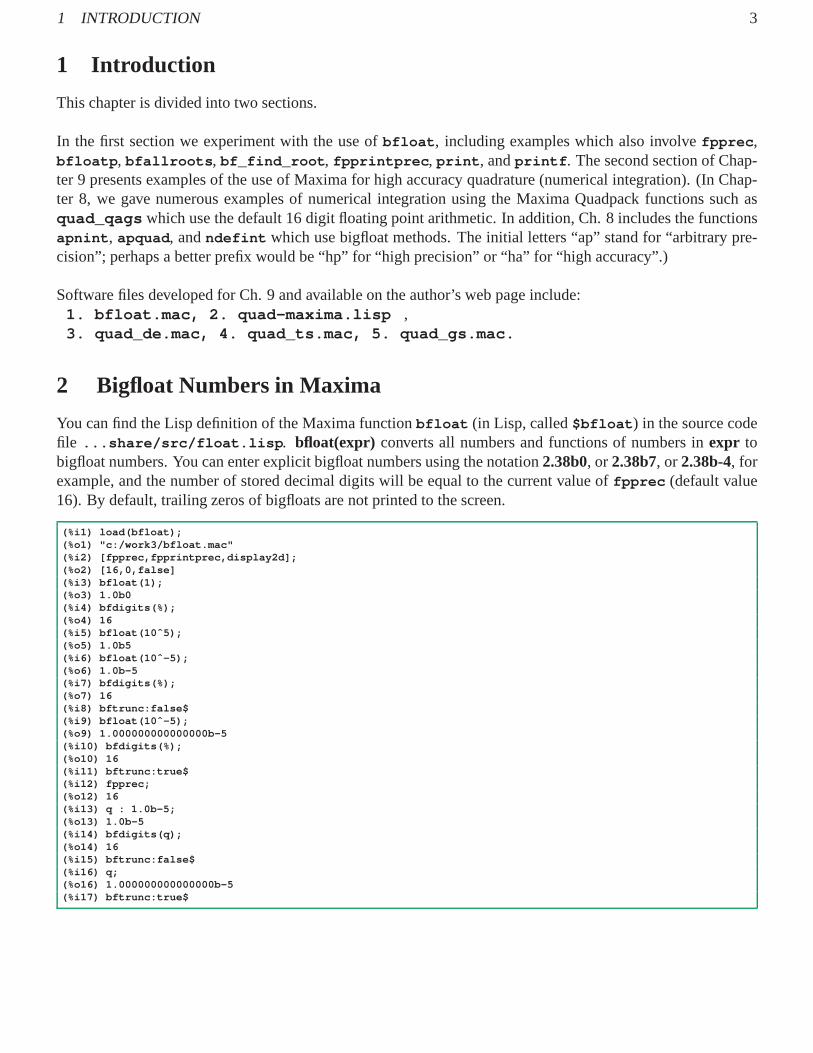
You can find the Lisp definition of the Maxima functionbfloat (in Lisp, called$bfloat ) in the source codefile ...share/src/float.lisp . bfloat(expr) converts all numbers and functions of numbers inexpr tobigfloat numbers. You can enter explicit bigfloat numbers using the notation2.38b0, or 2.38b7, or 2.38b-4, forexample, and the number of stored decimal digits will be equal to the current value offpprec (default value16). By default, trailing zeros of bigfloats are not printed to the screen.
(%i1) load(bfloat);(%o1) "c:/work3/bfloat.mac"(%i2) [fpprec,fpprintprec,display2d];(%o2) [16,0,false](%i3) bfloat(1);(%o3) 1.0b0(%i4) bfdigits(%);(%o4) 16(%i5) bfloat(10ˆ5);(%o5) 1.0b5(%i6) bfloat(10ˆ-5);(%o6) 1.0b-5(%i7) bfdigits(%);(%o7) 16(%i8) bftrunc:false$(%i9) bfloat(10ˆ-5);(%o9) 1.000000000000000b-5(%i10) bfdigits(%);(%o10) 16(%i11) bftrunc:true$(%i12) fpprec;(%o12) 16(%i13) q : 1.0b-5;(%o13) 1.0b-5(%i14) bfdigits(q);(%o14) 16(%i15) bftrunc:false$(%i16) q;(%o16) 1.000000000000000b-5(%i17) bftrunc:true$
2 BIGFLOAT NUMBERS IN MAXIMA 4
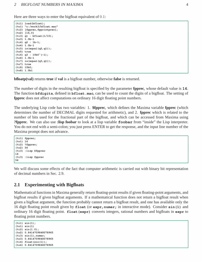
Here are three ways to enter the bigfloat equivalent of0.1:
(%i1) load(bfloat);(%o1) "c:/work3/bfloat.mac"(%i2) [fpprec,fpprintprec];(%o2) [16,0](%i3) q1 : bfloat(1/10);(%o3) 1.0b-1(%i4) q2 : 1b-1;(%o4) 1.0b-1(%i5) is(equal(q2,q1));(%o5) true(%i6) q3 : 10b0ˆ(-1);(%o6) 1.0b-1(%i7) is(equal(q3,q1));(%o7) true(%i8) 10b0;(%o8) 1.0b1
bfloatp(val) returnstrue if val is a bigfloat number, otherwisefalse is returned.
The number of digits in the resulting bigfloat is specified by the parameterfpprec, whose default value is16 .The functionbfdigits , defined inbfloat.mac , can be used to count the digits of a bigfloat. The setting offpprec does not affect computations on ordinary 16 digit floating point numbers.
The underlying Lisp code has two variables: 1.$fpprec, which defines the Maxima variablefpprec (whichdetermines the number of DECIMAL digits requested for arithmetic), and 2.fpprec which is related to thenumber of bits used for the fractional part of the bigfloat, and which can be accessed from Maxima using?fpprec. We can also use:lisp foobar to look at a lisp variablefoobar from “inside” the Lisp interpreter.You do not end with a semi-colon; you just press ENTER to get the response, and the input line number of theMaxima prompt does not advance.
(%i1) fpprec;(%o1) 16(%i2) ?fpprec;(%o2) 56(%i3) :lisp $fpprec16(%i3) :lisp fpprec56
We will discuss some effects of the fact that computer arithmetic is carried out with binary bit representationof decimal numbers in Sec. 2.9.
2.1 Experimenting with Bigfloats
Mathematical functions in Maxima generally return floating-point results if given floating-point arguments, andbigfloat results if given bigfloat arguments. If a mathematical function does not return a bigfloat result whengiven a bigfloat argument, the function probably cannot return a bigfloat result, and one has available only the16 digit floating point result given byfloat (or expr,numer; in interactive mode). Considersin(1) andordinary 16 digit floating point.float(expr) converts integers, rational numbers and bigfloats inexpr tofloating point numbers.
(%i1) sin(1);(%o1) sin(1)(%i2) sin(1.0);(%o2) 0.8414709848078965(%i3) sin(1),numer;(%o3) 0.8414709848078965(%i4) float(sin(1));(%o4) 0.8414709848078965

2 BIGFLOAT NUMBERS IN MAXIMA 5
Now considersin(1) and the use ofbfloat . The functionbfloat uses the current value of the globalparameterfpprec (which has the value 16 at normal startup) to return a bigfloatwith the correspondingnumber of digits. You can temporarily override the current global value offpprec (as shown below) withoutchanging that global value.
(%i5) fpprec;(%o5) 16(%i6) q : 1.0b0;(%o6) 1.0b0(%i7) bfdigits(q);(%o7) 16(%i8) q1 : sin(q);(%o8) 8.414709848078965b-1(%i9) q2 : bfloat(sin(1));(%o9) 8.414709848078965b-1(%i10) map (’bfdigits,[q1,q2]);(%o10) [16,16](%i11) is (equal (q1,q2));(%o11) true(%i12) q3 : bfloat(sin(1)), fpprec:20;(%o12) 8.4147098480789650665b-1(%i13) q4 : sin(1.0b0), fpprec : 20;(%o13) 8.4147098480789650665b-1(%i14) map (’bfdigits,[q3,q4]);(%o14) [20,20](%i15) is (equal (q3,q4));(%o15) true(%i16) fpprec;(%o16) 16
If we compute the absolute error of the 16 digit floating pointapproximation (which we callsfp below) tosin(1) , using as the “true value” the 20 digit approximation (s20 ), overriding the global value offpprec
temporarily as needed,
(%i17) s20 : bfloat (sin(1)), fpprec:20;(%o17) 8.4147098480789650665b-1(%i18) sfp : sin(1.0);(%o18) 0.8414709848078965(%i19) sfp_20 : bfloat(sfp),fpprec:20;(%o19) 8.4147098480789650488b-1(%i20) abs(sfp_20 - s20);(%o20) 0.0b0(%i21) abs(sfp_20 - s20), fpprec:20;(%o21) 1.7770751233395221114b-18(%i22) abs(sfp - s20), fpprec:20;(%o22) 1.7770751233395221114b-18
we see that we need to do the absolute error calculation using20 digit arithmetic, (as in step%i21 above) toget a sensible answer, and also that we get the same absolute error without first converting the 16 digit floatingpoint resultsfp to 20 digits, as we did in step%i19 above. The 20 digit bigfloatsfp_20 is no more accuratethan the 16 digit floating point numbersfp . Input %i22 involves one bigfloat number,s20 , and “bigfloatcontagion” occurs, which causes the floating point numbersfp to be promoted to 20 bigfloat digits, by addingbinary zeros, resulting in the decimal digits displayed in%o19above.
If we do a similar calculation with aglobal valueof fpprec set at the start, we should get the same results.However, the calculation is easier to do with the global value of fpprec set to 20, since if at least one of thenumbers involved is a bigfloat, all of the numbers are promoted to bigfloats (“bigfloat contagion”), and 20 digitarithmetic is then automatically used to get the result.
(%i23) fpprec;(%o23) 16(%i24) fpprec:20$
2 BIGFLOAT NUMBERS IN MAXIMA 6
(%i25) sfp : sin(1.0);(%o25) 0.8414709848078965(%i26) sfp_20 : bfloat(sfp);(%o26) 8.4147098480789650488b-1(%i27) s20 : bfloat (sin(1));(%o27) 8.4147098480789650665b-1(%i28) abs(sfp_20 - s20);(%o28) 1.7770751233395221114b-18(%i29) abs(sfp - s20);(%o29) 1.7770751233395221114b-18
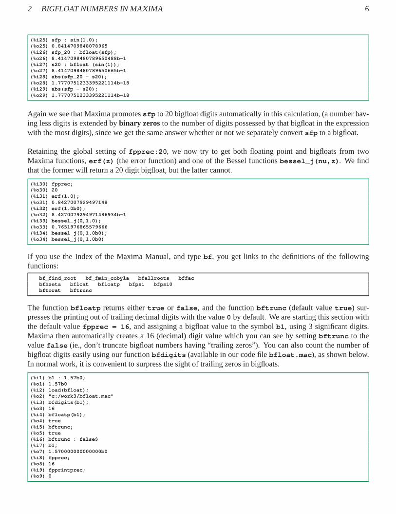
Again we see that Maxima promotessfp to 20 bigfloat digits automatically in this calculation, (a number hav-ing less digits is extended bybinary zeros to the number of digits possessed by that bigfloat in the expressionwith the most digits), since we get the same answer whether ornot we separately convertsfp to a bigfloat.
Retaining the global setting offpprec:20 , we now try to get both floating point and bigfloats from twoMaxima functions,erf(z) (the error function) and one of the Bessel functionsbessel_j(nu,z) . We findthat the former will return a 20 digit bigfloat, but the lattercannot.
(%i30) fpprec;(%o30) 20(%i31) erf(1.0);(%o31) 0.8427007929497148(%i32) erf(1.0b0);(%o32) 8.4270079294971486934b-1(%i33) bessel_j(0,1.0);(%o33) 0.7651976865579666(%i34) bessel_j(0,1.0b0);(%o34) bessel_j(0,1.0b0)
If you use the Index of the Maxima Manual, and typebf , you get links to the definitions of the followingfunctions:
bf_find_root bf_fmin_cobyla bfallroots bffacbfhzeta bfloat bfloatp bfpsi bfpsi0bftorat bftrunc
The functionbfloatp returns eithertrue or false , and the functionbftrunc (default valuetrue ) sur-presses the printing out of trailing decimal digits with thevalue0 by default. We are starting this section withthe default valuefpprec = 16 , and assigning a bigfloat value to the symbolb1, using 3 significant digits.Maxima then automatically creates a 16 (decimal) digit value which you can see by settingbftrunc to thevaluefalse (ie., don’t truncate bigfloat numbers having “trailing zeros”). You can also count the number ofbigfloat digits easily using our functionbfdigits (available in our code filebfloat.mac ), as shown below.In normal work, it is convenient to surpress the sight of trailing zeros in bigfloats.
(%i1) b1 : 1.57b0;(%o1) 1.57b0(%i2) load(bfloat);(%o2) "c:/work3/bfloat.mac"(%i3) bfdigits(b1);(%o3) 16(%i4) bfloatp(b1);(%o4) true(%i5) bftrunc;(%o5) true(%i6) bftrunc : false$(%i7) b1;(%o7) 1.570000000000000b0(%i8) fpprec;(%o8) 16(%i9) fpprintprec;(%o9) 0

2 BIGFLOAT NUMBERS IN MAXIMA 7
(%i10) floatnump(b1);(%o10) false(%i11) bfdigits(1.000000000000000b0);(%o11) 16
The description ofbftrunc from the Maxima Manual:
Option variable: bftruncDefault value: truebftrunc causes trailing zeroes in non-zero bigfloat number s
not to be displayed. Thus, if bftrunc is false, bfloat (1)displays as 1.000000000000000b0.Otherwise, this is displayed as 1.0b0.
Next consider obtaining numerical values ofcomplex expressions. First, 16 digit numbers usingfloat . Ourfirst attempt does not succeed:
(%i12) float(exp(%i * %pi/sin(1)));(%o12) 2.718281828459045ˆ((%i * %pi)/sin(1))
Here are two paths to what we want:
(%i13) float(exp(%i * %pi/sin(1))),numer;(%o13) (-0.5579061738629681 * %i)-0.8299040312985494(%i14) float( rectform (exp(%i * %pi/sin(1))));(%o14) (-0.5579061738629681 * %i)-0.8299040312985494
The bigfloat value is easier to get:
(%i15) fpprec;(%o15) 16(%i16) q : bfloat(exp(%i * %pi/sin(1)));(%o16) (-5.57906173862968b-1 * %i)-8.299040312985495b-1(%i17) bfloatp(q);(%o17) false(%i18) realpart(q);(%o18) -8.299040312985495b-1(%i19) imagpart(q);(%o19) -5.57906173862968b-1(%i20) imagpart(1.2b0);(%o20) 0
Note thatbfloat of a complex expression does not result in another bigfloat (as indicated by the return valueof bfloatp ), because of the presence of the symbol%i. In bfloat.mac the functionbfdigits is definedwhich gets around this difficulty by always working with the real part (or, if necessary, the imaginary part) ofan expression:
(%i1) load(bfloat);(%o1) "c:/work3/bfloat.mac"(%i2) q : bfloat(exp(%i * %pi/sin(1)));(%o2) (-5.57906173862968b-1 * %i)-8.299040312985495b-1(%i3) bfdigits(q);(%o3) 16(%i4) q : bfloat(exp(%i * %pi/sin(1))), fpprec:20;(%o4) (-5.579061738629679922b-1 * %i)-8.2990403129854944112b-1(%i5) bfdigits(q);(%o5) 20
The default value ofbftrunc (which istrue ) surpresses the printing of trailing (decimal) zeros, butbfdigits
still gives the correct number of decimal digits.
2 BIGFLOAT NUMBERS IN MAXIMA 8
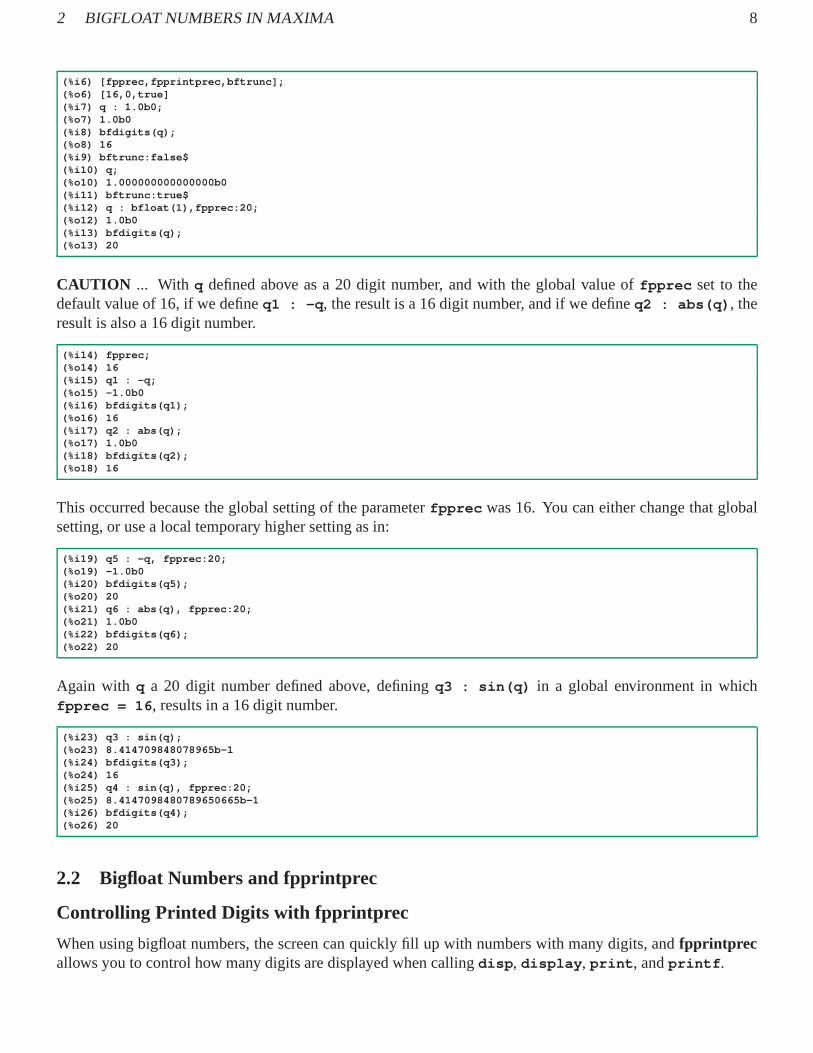
(%i6) [fpprec,fpprintprec,bftrunc];(%o6) [16,0,true](%i7) q : 1.0b0;(%o7) 1.0b0(%i8) bfdigits(q);(%o8) 16(%i9) bftrunc:false$(%i10) q;(%o10) 1.000000000000000b0(%i11) bftrunc:true$(%i12) q : bfloat(1),fpprec:20;(%o12) 1.0b0(%i13) bfdigits(q);(%o13) 20
CAUTION ... With q defined above as a 20 digit number, and with the global value offpprec set to thedefault value of 16, if we defineq1 : -q , the result is a 16 digit number, and if we defineq2 : abs(q) , theresult is also a 16 digit number.
(%i14) fpprec;(%o14) 16(%i15) q1 : -q;(%o15) -1.0b0(%i16) bfdigits(q1);(%o16) 16(%i17) q2 : abs(q);(%o17) 1.0b0(%i18) bfdigits(q2);(%o18) 16
This occurred because the global setting of the parameterfpprec was 16. You can either change that globalsetting, or use a local temporary higher setting as in:
(%i19) q5 : -q, fpprec:20;(%o19) -1.0b0(%i20) bfdigits(q5);(%o20) 20(%i21) q6 : abs(q), fpprec:20;(%o21) 1.0b0(%i22) bfdigits(q6);(%o22) 20
Again with q a 20 digit number defined above, definingq3 : sin(q) in a global environment in whichfpprec = 16 , results in a 16 digit number.
(%i23) q3 : sin(q);(%o23) 8.414709848078965b-1(%i24) bfdigits(q3);(%o24) 16(%i25) q4 : sin(q), fpprec:20;(%o25) 8.4147098480789650665b-1(%i26) bfdigits(q4);(%o26) 20
2.2 Bigfloat Numbers and fpprintprec
Controlling Printed Digits with fpprintprec
When using bigfloat numbers, the screen can quickly fill up with numbers with many digits, andfpprintprecallows you to control how many digits are displayed when calling disp , display , print , andprintf .

2 BIGFLOAT NUMBERS IN MAXIMA 9
For bigfloat numbers, whenfpprintprec has a value greater than2 and less thanfpprec, the number of digitsprinted is equal tofpprintprec . If fpprintprec = 0 then all the bigfloat digits are printed.fpprintprec cannotbe 1. The setting offpprintprec does not affect the precision of the bigfloat arithmetic carried out, only thesetting offpprec matters.
We can use local temporary values offpprintprec andfpprec in interactive work.
(%i1) load(bfloat);(%o1) "c:/work3/bfloat.mac"(%i2) [fpprec,fpprintprec];(%o2) [16,0](%i3) q : integrate(exp(x),x,-1,1);(%o3) %e-%eˆ-1(%i4) q : bfloat(q),fpprec : 45;(%o4) 2.35040238728760291376476370119120163031143596 b0(%i5) bfdigits(q);(%o5) 45(%i6) print (q),fpprintprec : 12$2.35040238728b0(%i7) fpprec;(%o7) 16(%i8) print (q),fpprintprec : 15$2.3504023872876b0(%i9) print (q),fpprintprec : 16$2.35040238728760291376476370119120163031143596b0(%i10) print (q),fpprintprec : 17$2.35040238728760291376476370119120163031143596b0(%i11) print (q),fpprec:18, fpprintprec : 17$2.3504023872876029b0(%i12) print (q),fpprec:19, fpprintprec : 18$2.35040238728760291b0(%i13) fpprintprec;(%o13) 0(%i14) print(q)$2.35040238728760291376476370119120163031143596b0
Either or both of the parametersfpprec andfpprintprec can be used as local variables inside a function or inan assignment statement defined usingblock, and set to local value(s) which do not affect the global setting.If used in a function, such locally defined values offpprec andfpprintprec govern the bigfloat calculationsin that function and in any functions called by that function, and in any third layer functions called by thesecondary layer functions, etc.
Here is a simple pedagogical example of usingblock to produce an assignment statement (not a function).(Recall that ourmaxima-init.mac file has the linedisplay2d:false ).
(%i15) [fpprec,fpprintprec];(%o15) [16,0](%i16) piby2 : block([fpprintprec,fpprec:30,val],
val:bfloat(%pi/2),fpprintprec:8,disp (val),display (val),print(" val = ",val),print(" bfdigits(val) = ", bfdigits(val) ),val);
1.5707963b0
val = 1.5707963b0
val = 1.5707963b0bfdigits(val) = 30
(%o16) 1.57079632679489661923132169164b0(%i17) bfdigits(piby2);(%o17) 30(%i18) [fpprec,fpprintprec];(%o18) [16,0]

2 BIGFLOAT NUMBERS IN MAXIMA 10
An alternative assignment statement which does not useblock but does use local temporary values offpprintprec andfpprec (and has the defect of introducing a global value for the symbol val ) is:
(%i19) piby2 : (val:bfloat(%pi/2),disp (val),display (val),print(" val = ",val),print(" bfdigits(val) = ", bfdigits(val) ),val ), fpprintp rec:8, fpprec:30;
1.5707963b0
val = 1.5707963b0
val = 1.5707963b0bfdigits(val) = 30
(%o19) 1.57079632679489661923132169164b0(%i20) piby2;(%o20) 1.57079632679489661923132169164b0(%i21) bfdigits(piby2);(%o21) 30(%i22) val;(%o22) 1.57079632679489661923132169164b0
Next we illustrate a function passing both a bigfloat number as well as local values offpprec andfpprintprecto a second function. Here functionf1 is designed to call functionf2 :
(%i23) f2(w) := block([v2 ],print (" in function f2 "),display([w,fpprec,fpprintprec]),print (" bfdigits(w) = ", bfdigits(w)),v2 : sin(w),print (" v2 = sin(w) = ", v2),print (" bfdigits(v2) = ", bfdigits(v2) ),print(" "),v2 )$
(%i24) f1(x, fpp, fpprt) := block([fpprintprec,fpprec:fp p,v1],fpprintprec:fpprt,display([x,fpprec,fpprintprec]),print(" in function f1, call f2(x) "),v1 : f2(bfloat(x))ˆ2,print(" back in f1, v1 = sin(x)ˆ2 = ",v1),print(" bfdigits(v1) = ",bfdigits(v1)),v1 )$
And here we callf1 with valuesx = 0.5, fpp = 30, fpprt = 8 :
(%i25) q : f1(0.5,30,8);[x,fpprec,fpprintprec] = [0.5,30,8]
in function f1, call f2(x)in function f2
[w,fpprec,fpprintprec] = [5.0b-1,30,8]
bfdigits(w) = 30v2 = sin(w) = 4.7942553b-1
bfdigits(v2) = 30
back in f1, v1 = sin(x)ˆ2 = 2.2984884b-1bfdigits(v1) = 30
(%o25) 2.29848847065930141299531696279b-1(%i26) q;(%o26) 2.29848847065930141299531696279b-1(%i27) bfdigits(q);(%o27) 30(%i28) [fpprec,fpprintprec];(%o28) [16,0]
We see that the called functionf2 maintainsthe values offpprec andfpprintprec which exist in the call-ing functionf1 .

2 BIGFLOAT NUMBERS IN MAXIMA 11
Bigfloat numbers are “contagious” in the sense that, for example, multiplying (or adding) an integer or ordinaryfloat number with a bigfloat results in a bigfloat number. In theabove examplesin(w) is a bigfloat sincew isone.
(%i29) fpprec:20$(%i30) q : bfloat(2);(%o30) 2.0b0(%i31) bfdigits(q);(%o31) 20(%i32) q1 : 1 + q;(%o32) 3.0b0(%i33) bfdigits(q1);(%o33) 20(%i34) q2 : 1.0 + q;(%o34) 3.0b0(%i35) bfdigits(q2);(%o35) 20(%i36) q3 : sin(q2);(%o36) 1.411200080598672221b-1(%i37) bfdigits(q3);(%o37) 20
The Maxima symbol%pi is not automatically converted to a numerical value by contagion and an extra use ofbfloat does the conversion.
(%i38) a : 2.38b-1$(%i39) a;(%o39) 2.38b-1(%i40) bfdigits(a);(%o40) 20(%i41) q4 : exp(%pi * a);(%o41) %eˆ(2.38b-1 * %pi)(%i42) q4 : bfloat(q4);(%o42) 2.1121345085033606761b0(%i43) bfdigits(q4);(%o43) 20
The following example illustrates how the setting offpprec can affect what is printed to the screen when doingbigfloat arithmetic.
(%i44) fpprec;(%o44) 20(%i45) q1 : bfloat(1);(%o45) 1.0b0(%i46) bfdigits(q1);(%o46) 20(%i47) q2 : bfloat(10ˆ(-25));(%o47) 1.0b-25(%i48) bfdigits(q2);(%o48) 20(%i49) q3 : q1 + q2;(%o49) 1.0b0(%i50) q3, fpprec:25;(%o50) 1.0b0(%i51) q3, fpprec:26;(%o51) 1.0b0(%i52) q3 : q1 + q2,fpprec:26;(%o52) 1.0000000000000000000000001b0(%i53) bfdigits(q3);(%o53) 26
Note that1b-25 is the bigfloat version of10−25. In the case above the value offpprec is large enough to seethe effect of the bigfloat addition.

2 BIGFLOAT NUMBERS IN MAXIMA 12
2.3 Using print with Bigfloats
In Sec. 2.2 we described the relations between the settings of fpprec andfpprintprec and we repeat some ofthat discussion here. Once you have generated a bigfloat withsome precision, it is convenient to be able tocontrol how many digits are displayed. We start with the use of print . If you start with the global defaultvalue of16 for fpprec and the default value of0 for fpprintprec , you can use a simple one line command fora low number of digits, as shown in the following. We first define a bigfloatq to havefpprec = 45 digits ofprecision:
(%i1) load(bfloat);(%o1) "c:/work3/bfloat.mac"(%i2) [fpprec,fpprintprec];(%o2) [16,0](%i3) integrate(exp(x),x,-1,1);(%o3) %e-%eˆ-1(%i4) q : bfloat(%),fpprec : 45;(%o4) 2.35040238728760291376476370119120163031143596 b0(%i5) bfdigits(q);(%o5) 45
We then useprint with fpprintprec to get increasing numbers of digits on the screen. When the tem-porary value offpprintprec is equal to the global value offpprec (here 16), all 45 digits are printed out.To get only 16 digits printed to the screen, you need to set a local temporary value offpprec greater than orequal to 17.
(%i6) print(q),fpprintprec:5$2.3504b0(%i7) print(q),fpprintprec:15$2.3504023872876b0(%i8) print(q),fpprintprec:16$2.35040238728760291376476370119120163031143596b0(%i9) print(q),fpprintprec:0$2.35040238728760291376476370119120163031143596b0(%i10) print(q),fpprec:21,fpprintprec:20$2.3504023872876029137b0(%i11) print(q),fpprec:17,fpprintprec:16$2.350402387287602b0(%i12) [fpprec,fpprintprec];(%o12) [16,0]
A functionbfprint , defined inbfloat.mac with the code
bfprint(smsg,xbf,fpp) :=block([fpprec, fpprintprec ],
fpprec : fpp + 1,fpprintprec : fpp,print (smsg, xbf))$
can be used to implement this idea:
(%i13) bfprint(" q16 = ",q,16)$q16 = 2.350402387287602b0
(%i14) bfprint(" q20 = ",q,20)$q20 = 2.3504023872876029137b0
2 BIGFLOAT NUMBERS IN MAXIMA 13
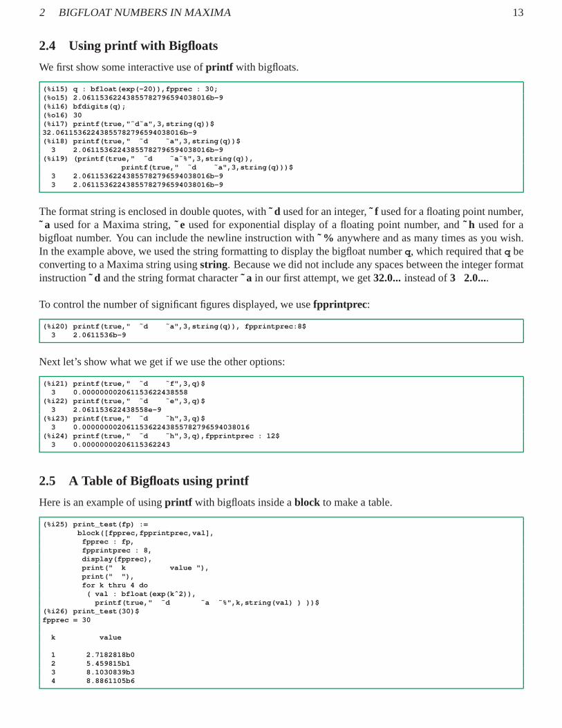
2.4 Using printf with Bigfloats
We first show some interactive use ofprintf with bigfloats.
(%i15) q : bfloat(exp(-20)),fpprec : 30;(%o15) 2.06115362243855782796594038016b-9(%i16) bfdigits(q);(%o16) 30(%i17) printf(true,"˜d˜a",3,string(q))$32.06115362243855782796594038016b-9(%i18) printf(true," ˜d ˜a",3,string(q))$
3 2.06115362243855782796594038016b-9(%i19) (printf(true," ˜d ˜a˜%",3,string(q)),
printf(true," ˜d ˜a",3,string(q)))$3 2.06115362243855782796594038016b-93 2.06115362243855782796594038016b-9
The format string is enclosed in double quotes, with˜ d used for an integer,˜ f used for a floating point number,˜ a used for a Maxima string,̃e used for exponential display of a floating point number, and˜ h used for abigfloat number. You can include the newline instruction with ˜ % anywhere and as many times as you wish.In the example above, we used the string formatting to display the bigfloat numberq, which required thatq beconverting to a Maxima string usingstring. Because we did not include any spaces between the integer formatinstruction˜ d and the string format character˜ a in our first attempt, we get32.0...instead of3 2.0....
To control the number of significant figures displayed, we usefpprintprec :
(%i20) printf(true," ˜d ˜a",3,string(q)), fpprintprec:8 $3 2.0611536b-9
Next let’s show what we get if we use the other options:
(%i21) printf(true," ˜d ˜f",3,q)$3 0.000000002061153622438558
(%i22) printf(true," ˜d ˜e",3,q)$3 2.061153622438558e-9
(%i23) printf(true," ˜d ˜h",3,q)$3 0.00000000206115362243855782796594038016
(%i24) printf(true," ˜d ˜h",3,q),fpprintprec : 12$3 0.00000000206115362243
2.5 A Table of Bigfloats using printf
Here is an example of usingprintf with bigfloats inside ablock to make a table.
(%i25) print_test(fp) :=block([fpprec,fpprintprec,val],
fpprec : fp,fpprintprec : 8,display(fpprec),print(" k value "),print(" "),for k thru 4 do
( val : bfloat(exp(kˆ2)),printf(true," ˜d ˜a ˜%",k,string(val) ) ))$
(%i26) print_test(30)$fpprec = 30
k value
1 2.7182818b02 5.459815b13 8.1030839b34 8.8861105b6

2 BIGFLOAT NUMBERS IN MAXIMA 14
Note the crucial use of the newline instruction˜ % to get the table output. Many examples ofprintf can befound in the Maxima manual under the index listingprintf and many more in..../share/stringproc/rtestprintf.mac .
We can useprintf (for headings and space) instead ofprint with an alternative version.
(%i27) print_test2(fp) :=block([fpprec,fpprintprec,val],
fpprec : fp,fpprintprec : 8,display(fpprec),printf(true,"˜% ˜a ˜a ˜%˜%",k,value),for k thru 4 do
( val : bfloat(exp(kˆ2)),printf(true," ˜d ˜a ˜%",k,string(val) ) ))$
Here we try out the alternative function withfp = 30 :
(%i28) print_test2(30)$fpprec = 30
k value
1 2.7182818b02 5.459815b13 8.1030839b34 8.8861105b6
2.6 Adding Bigfloats Having Differing Accuracy
If A and B are bigfloats with different accuracy, the accuracy (correct digits) of the sum(A + B) is theaccuracy (correct digits) of the least accurate number. As an example, letpi50 be an approximation toπaccurate to 50 digits, and letpi100 be an approximation toπ accurate to 100 digits. The sum,pisum , is onlyaccurate to 50 digits, as seen by a comparison with the value of 2 π calculated using 100 digit arithmetic( twopi ) which is taken as the “true value” when calculating absolute error.
(%i1) fpprintprec:8$(%i2) fpprec;(%o2) 16(%i3) pi100 : bfloat(%pi),fpprec:100;(%o3) 3.1415926b0(%i4) pi50 : bfloat(%pi),fpprec:50;(%o4) 3.1415926b0(%i5) abs(pi50 - pi100),fpprec:101;(%o5) 1.0106957b-51(%i6) twopi : bfloat(2 * %pi),fpprec:100;(%o6) 6.2831853b0(%i7) pisum : pi50 + pi100,fpprec:100;(%o7) 6.2831853b0(%i8) pisum - twopi,fpprec:101;(%o8) 1.0106957b-51
2 BIGFLOAT NUMBERS IN MAXIMA 15
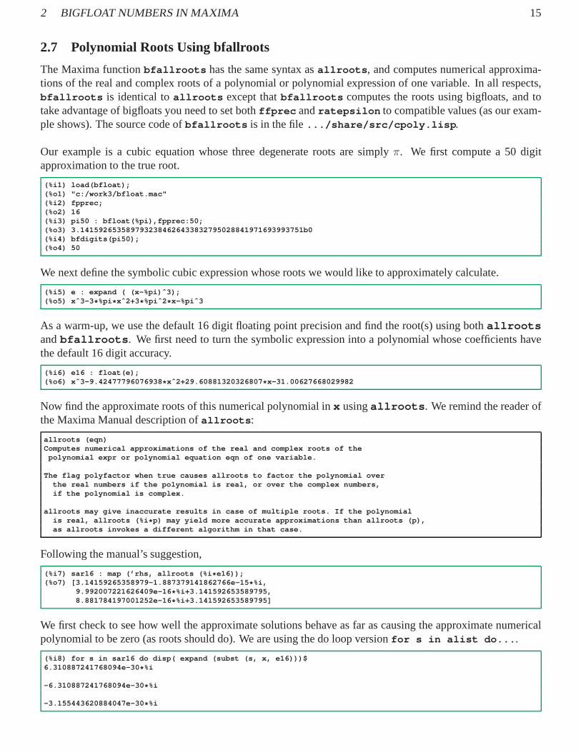
2.7 Polynomial Roots Using bfallroots
The Maxima functionbfallroots has the same syntax asallroots , and computes numerical approxima-tions of the real and complex roots of a polynomial or polynomial expression of one variable. In all respects,bfallroots is identical toallroots except thatbfallroots computes the roots using bigfloats, and totake advantage of bigfloats you need to set bothffprec andratepsilon to compatible values (as our exam-ple shows). The source code ofbfallroots is in the file.../share/src/cpoly.lisp .
Our example is a cubic equation whose three degenerate rootsare simplyπ. We first compute a 50 digitapproximation to the true root.
(%i1) load(bfloat);(%o1) "c:/work3/bfloat.mac"(%i2) fpprec;(%o2) 16(%i3) pi50 : bfloat(%pi),fpprec:50;(%o3) 3.14159265358979323846264338327950288419716939 93751b0(%i4) bfdigits(pi50);(%o4) 50
We next define the symbolic cubic expression whose roots we would like to approximately calculate.
(%i5) e : expand ( (x-%pi)ˆ3);(%o5) xˆ3-3 * %pi * xˆ2+3 * %piˆ2 * x-%piˆ3
As a warm-up, we use the default 16 digit floating point precision and find the root(s) using bothallrootsandbfallroots . We first need to turn the symbolic expression into a polynomial whose coefficients havethe default 16 digit accuracy.
(%i6) e16 : float(e);(%o6) xˆ3-9.42477796076938 * xˆ2+29.60881320326807 * x-31.00627668029982
Now find the approximate roots of this numerical polynomial in x usingallroots . We remind the reader ofthe Maxima Manual description ofallroots :
allroots (eqn)Computes numerical approximations of the real and complex r oots of the
polynomial expr or polynomial equation eqn of one variable.
The flag polyfactor when true causes allroots to factor the p olynomial overthe real numbers if the polynomial is real, or over the comple x numbers,if the polynomial is complex.
allroots may give inaccurate results in case of multiple roo ts. If the polynomialis real, allroots (%i * p) may yield more accurate approximations than allroots (p) ,as allroots invokes a different algorithm in that case.
Following the manual’s suggestion,
(%i7) sar16 : map (’rhs, allroots (%i * e16));(%o7) [3.14159265358979-1.887379141862766e-15 * %i,
9.992007221626409e-16 * %i+3.141592653589795,8.881784197001252e-16 * %i+3.141592653589795]
We first check to see how well the approximate solutions behave as far as causing the approximate numericalpolynomial to be zero (as roots should do). We are using the doloop versionfor s in alist do... .
(%i8) for s in sar16 do disp( expand (subst (s, x, e16)))$6.310887241768094e-30 * %i
-6.310887241768094e-30 * %i
-3.155443620884047e-30 * %i

2 BIGFLOAT NUMBERS IN MAXIMA 16
which is very good root behavior. The appearance of%i is due to our askingallroots for the roots of%i* e15 :
(%i9) for s in sar16 do disp( expand (subst (s, x, %i * e16)))$-6.310887241768094e-30
6.310887241768094e-30
3.155443620884047e-30
We next compare the approximate roots (taking realpart) to pi50.
(%i10) for s in sar16 do disp (pi50 - realpart(s))$3.663735981263017b-15
-1.665334536937735b-15
-1.665334536937735b-15
The above accuracy in findingπ corresponds to the default floating point precision being used.
Retaining the default 16 digit precision, we try outbfallroots . The Manual has the description
bfallroots (eqn)Computes numerical approximations of the real and complex r oots
of the polynomial expr or polynomial equation eqn of one vari able.
In all respects, bfallroots is identical to allroots except that bfallrootscomputes the roots using bigfloats. See allroots for more in formation
(%i11) sbfar16 : map (’rhs, bfallroots (%i * e16));(%o11) [3.141592653589788b0-1.207367539279858b-15 * %i,
5.967448757360216b-16 * %i+3.141592653589797b0,6.106226635438361b-16 * %i+3.141592653589795b0]
We then again check the roots against the expression:
(%i12) for s in sbfar16 do disp( expand (subst (s,x,e16)))$7.888609052210118b-31 * %i+2.664535259100376b-15
1.332267629550188b-15
1.332267629550188b-15-3.944304526105059b-31 * %i
and compare the accuracy against our “true value”.
(%i13) for s in sbfar16 do disp (pi50 - realpart(s))$5.662137425588298b-15
-3.774758283725532b-15
-1.554312234475219b-15
Thus we see thatbfallroots provides no increased accuracy unless we setfpprec andratepsilon tovalues which will cause Maxima to use higher precision.
In order to demonstrate the necessity of settingratepsilon , we first try outbfallroots using only thefpprec setting. Let’s try to solve for the roots with 40 digit accuracy, first converting the symbolic cubic to anumerical cubic with coefficients having 40 digit accuracy.

2 BIGFLOAT NUMBERS IN MAXIMA 17
(%i14) e;(%o14) xˆ3-3 * %pi * xˆ2+3 * %piˆ2 * x-%piˆ3(%i15) fpprec:40$(%i16) e40 : bfloat(e);(%o16) xˆ3-9.424777960769379715387930149838508652592 b0* xˆ2
+2.960881320326807585650347299962845340594b1 * x-3.100627668029982017547631506710139520223b1
The coefficients are now bigfloats, with the tell-taleb0 or b1 power of ten factor attached to the end.
Now we seek the roots usingbfallroots , using 40 digit arithmetic. The global parameterbftorat bydefault has the valuefalse , which causes the parameterratepsilon (default value =2.0e-15 ) to governthe tolerance for the conversion of floats and bigfloats to rational numbers. The code filebfloat.mac has theline ratprint:false , so we are restoring the Maxima default (true ) in order to monitor the conversion offloats and bigfloats to rational numbers here.
(%i17) bftorat;(%o17) false(%i18) ratprint:true$(%i19) ratepsilon;(%o19) 2.0e-15(%i20) sbfar40 : map (’rhs, bfallroots (%i * e40));‘rat’ replaced -3.10062766802998201754763150671013952 0223B1
by -314736901/10150748 = -3.10062766802998163288065076 5835187712275B1‘rat’ replaced 2.960881320326807585650347299962845340 594B1
by 81466873/2751440 = 2.960881320326810688221440409385 630796965B1‘rat’ replaced -9.42477796076937971538793014983850865 2592B0
by -245850922/26085593 = -9.42477796076937948084983155 2612202452135B0(%o20) [4.067836769152171502691170240490135999242b-5 * %i
+3.141616139025696356200813766622571203502b0,3.14154568271798676844820401936706004245b0
-1.548009312010808033271429697254614341017b-36 * %i,3.141616139025696356200813766622571206183b0
-4.067836769152171502691170240489981198311b-5 * %i]
Check the 40 digit expression using these roots
(%i21) for s in sbfar40 do disp (expand (subst (s,x,e40)))$(-1.322021252743128684063725037210791852918b-18 * %i)
-1.036323768523864674946697445152469123351b-13
(-1.024594606934776373480991399282522431152b-44 * %i)-1.036300870684467447465412546012022927675b-13
1.322021252743128684063725037210791852918b-18 * %i-1.036323768523864674946697408418270660154b-13
and check the closeness of the roots to the “true value”,
(%i22) for s in sbfar40 do disp (pi50 - realpart(s))$-2.348543590311773817038334306831930475506b-5
4.697087180647001443936391244284174701383b-5
-2.348543590311773817038334306832198580053b-5
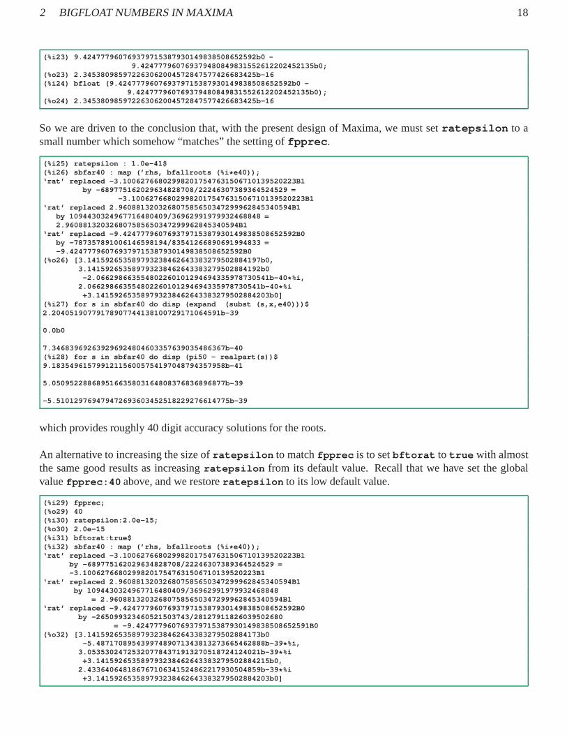
which are really poor results, apparently caused by inaccurate rat replacement of decimal coefficients byratios of whole numbers. Look, for example, at the third rat replacement above and its difference from theactual 40 digit accurate number (becausefpprec now has the global value 40, we don’t need to wrap thebigfloat arithmetic withbfloat ):
2 BIGFLOAT NUMBERS IN MAXIMA 18
(%i23) 9.424777960769379715387930149838508652592b0 -9.424777960769379480849831552612202452135b0;
(%o23) 2.345380985972263062004572847577426683425b-16(%i24) bfloat (9.424777960769379715387930149838508652 592b0 -
9.424777960769379480849831552612202452135b0);(%o24) 2.345380985972263062004572847577426683425b-16
So we are driven to the conclusion that, with the present design of Maxima, we must setratepsilon to asmall number which somehow “matches” the setting offpprec .
(%i25) ratepsilon : 1.0e-41$(%i26) sbfar40 : map (’rhs, bfallroots (%i * e40));‘rat’ replaced -3.10062766802998201754763150671013952 0223B1
by -689775162029634828708/22246307389364524529 =-3.100627668029982017547631506710139520223B1
‘rat’ replaced 2.960881320326807585650347299962845340 594B1by 1094430324967716480409/36962991979932468848 =2.960881320326807585650347299962845340594B1
‘rat’ replaced -9.42477796076937971538793014983850865 2592B0by -787357891006146598194/83541266890691994833 =-9.424777960769379715387930149838508652592B0
(%o26) [3.141592653589793238462643383279502884197b0,3.141592653589793238462643383279502884192b0
-2.066298663554802260101294694335978730541b-40 * %i,2.066298663554802260101294694335978730541b-40 * %i
+3.141592653589793238462643383279502884203b0](%i27) for s in sbfar40 do disp (expand (subst (s,x,e40)))$2.20405190779178907744138100729171064591b-39
0.0b0
7.346839692639296924804603357639035486367b-40(%i28) for s in sbfar40 do disp (pi50 - realpart(s))$9.183549615799121156005754197048794357958b-41
5.050952288689516635803164808376836896877b-39
-5.510129769479472693603452518229276614775b-39
which provides roughly 40 digit accuracy solutions for the roots.
An alternative to increasing the size ofratepsilon to matchfpprec is to setbftorat to true with almostthe same good results as increasingratepsilon from its default value. Recall that we have set the globalvaluefpprec:40 above, and we restoreratepsilon to its low default value.
(%i29) fpprec;(%o29) 40(%i30) ratepsilon:2.0e-15;(%o30) 2.0e-15(%i31) bftorat:true$(%i32) sbfar40 : map (’rhs, bfallroots (%i * e40));‘rat’ replaced -3.10062766802998201754763150671013952 0223B1
by -689775162029634828708/22246307389364524529 =-3.100627668029982017547631506710139520223B1
‘rat’ replaced 2.960881320326807585650347299962845340 594B1by 1094430324967716480409/36962991979932468848
= 2.960881320326807585650347299962845340594B1‘rat’ replaced -9.42477796076937971538793014983850865 2592B0
by -265099323460521503743/28127911826039502680= -9.424777960769379715387930149838508652591B0
(%o32) [3.141592653589793238462643383279502884173b0-5.48717089543997489071343813273665462888b-39 * %i,
3.053530247253207784371913270518724124021b-39 * %i+3.141592653589793238462643383279502884215b0,
2.433640648186767106341524862217930504859b-39 * %i+3.141592653589793238462643383279502884203b0]
2 BIGFLOAT NUMBERS IN MAXIMA 19
(%i33) for s in sbfar40 do disp (expand (subst (s,x,e40)))$0.0b0
4.318084277547222312693175931400199785558b-78 * %i-2.20405190779178907744138100729171064591b-39
-2.159042138773611156346587965700099892779b-78 * %i
(%i34) for s in sbfar40 do disp (pi50 - realpart(s))$2.378539350491972379405490337035637738711b-38
-1.772425075849230383109110560030417311086b-38
-5.693800761795455116723567602170252501934b-39
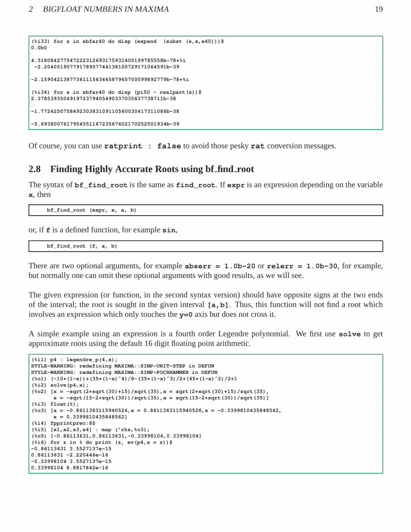
Of course, you can useratprint : false to avoid those peskyrat conversion messages.
2.8 Finding Highly Accurate Roots using bffind root
The syntax ofbf_find_root is the same asfind_root . If expr is an expression depending on the variablex , then
bf_find_root (expr, x, a, b)
or, if f is a defined function, for examplesin ,
bf_find_root (f, a, b)
There are two optional arguments, for exampleabserr = 1.0b-20 or relerr = 1.0b-30 , for example,but normally one can omit these optional arguments with goodresults, as we will see.
The given expression (or function, in the second syntax version) should have opposite signs at the two endsof the interval; the root is sought in the given interval[a,b] . Thus, this function will not find a root whichinvolves an expression which only touches they=0 axis but does not cross it.
A simple example using an expression is a fourth order Legendre polynomial. We first usesolve to getapproximate roots using the default 16 digit floating point arithmetic.
(%i1) p4 : legendre_p(4,x);STYLE-WARNING: redefining MAXIMA::SIMP-UNIT-STEP in DEF UNSTYLE-WARNING: redefining MAXIMA::SIMP-POCHHAMMER in DE FUN(%o1) (-10 * (1-x))+(35 * (1-x)ˆ4)/8-(35 * (1-x)ˆ3)/2+(45 * (1-x)ˆ2)/2+1(%i2) solve(p4,x);(%o2) [x = -sqrt(2 * sqrt(30)+15)/sqrt(35),x = sqrt(2 * sqrt(30)+15)/sqrt(35),
x = -sqrt(15-2 * sqrt(30))/sqrt(35),x = sqrt(15-2 * sqrt(30))/sqrt(35)](%i3) float(%);(%o3) [x = -0.8611363115940526,x = 0.8611363115940526,x = -0.3399810435848562,
x = 0.3399810435848562](%i4) fpprintprec:8$(%i5) [x1,x2,x3,x4] : map (’rhs,%o3);(%o5) [-0.86113631,0.86113631,-0.33998104,0.33998104 ](%i6) for z in % do print (z, ev(p4,x = z))$-0.86113631 3.5527137e-150.86113631 -2.220446e-16-0.33998104 3.5527137e-150.33998104 8.8817842e-16

2 BIGFLOAT NUMBERS IN MAXIMA 20
Now we focus on getting the value of the root near0.34 using 40 digit arithmetic withbf_find_root .
(%i7) fpprec : 40$(%i8) rt : bf_find_root(p4,x,0.3,0.4);(%o8) 3.3998104b-1(%i9) p4,x = rt;(%o9) 3.6734198b-40(%i10) fpprintprec : 0$(%i11) rt;(%o11) 3.399810435848562648026657591032446872006b-1
A simple example using a defined function isf(x) = 1 − 2 x/3 − sin(x), which has a root which can begraphically located using
(%i10) plot2d([1-2 * x/3 - sin(x),[discrete,[[0,0],[1,0]]]],[x,0,1],[style,[lines,2]],[legend,false])$
which produces the plot (after toggling on the grid):
Figure 1:f(x) = 1− 2 x/3− sin(x)
Placing the cursor at the position of the curve crossing the x-axis, we findx-root = 0.62 roughly. We canthen find a more accurate value:
(%i1) g(x) := 1 - 2 * x/3 - sin(x)$(%i2) g(0.62);(%o2) 0.005631506129361585(%i3) fpprec : 40$(%i4) rt : bf_find_root(g,0.6,0.64);(%o4) 6.2380651896161231998761522616487920495b-1(%i5) g(rt);(%o5) -2.29588740394978028900143854926219858949b-41
2.9 Bigfloat Number Gaps and Binary Arithmetic
The value of the integerfpprec determines the number of DECIMAL digits to be retained in thesubsequentarithmetic. In fact, theactual arithmetic is carried out withbinary arithmetic . Due to the inevitably finitenumber of binary bits used to represent a floating point number or a bigfloat, there will be a range of floatingpoint numbers (or bigfloats) which are not recognised as different.

2 BIGFLOAT NUMBERS IN MAXIMA 21
The internal Lisp representation of a bigfloat is
( (BIGFLOAT SIMP precision) mantissa exponent )
in which precision is an integer which is related to the number of bits of precision in the mantissa (thenumber of bits in the “fractional part”[see below] of a bigfloat isprecision - 1 ), and this number canbe retrieved from the console prompt using?fpprec .
Here is an example of settingfpprec to the integer 2:
(%i1) fpprec:2$(%i2) ?fpprec;(%o2) 9(%i3) :lisp $fpprec2(%i3) :lisp fpprec9
so if we ask for 2decimal digits of precision (two digit arithmetic, with the answer rounded to 2 digits), Lispuses 8 bits of precision in the fractional part of the bigfloat.
The “exponent” is a signed integer representing the scale ofthe number.
The “mantissa” is a signed integer used to represent a fractional portion defined by
fraction = mantissa / 2ˆ(precision)
such that the actual decimal number is the product
fraction * 2ˆ(exponent)
We start with a bigfloat which is represented by both a zero exponent and a zero mantissa (and hence a zerofraction), retainingfpprec=2 for now.
(%i3) x : 0.0b0$(%i4) :lisp $x;((BIGFLOAT SIMP 9) 0 0)
Here is another example
(%i4) x : 1.0b0;(%o4) 1.0b0(%i5) ?print(x);((BIGFLOAT SIMP 9) 256 1)(%o5) 1.0b0(%i6) :lisp $x((BIGFLOAT SIMP 9) 256 1)
We can also define a value ofx inside the Lisp interpreter. (We are usingmsetq instead ofsetq or setf toavoid useless noise from the SBCL Lisp interpreter.)
(%i6) :lisp (msetq $x ’((BIGFLOAT SIMP 9) 0 0))((BIGFLOAT SIMP 9) 0 0)(%i6) x;(%o6) 0.0b0

2 BIGFLOAT NUMBERS IN MAXIMA 22
If we increase the mantissa integer by 1, we get2.0b-3 .
(%i7) :lisp (msetq $u ’((BIGFLOAT SIMP 9) 1 0))((BIGFLOAT SIMP 9) 1 0)(%i7) u;(%o7) 2.0b-3
Consider the gap around the numberx:bfloat(2/3) for the casefpprec = 4. We will find that?fpprec has thevalue16and that Maxima behaves as if (for this case) the fractional part of a bigfloat number is represented bythe state of a system consisting of18 binary bits.
Let u = 2−18. If we let x1 = x+ u we get a number which is treated as having a nonzero difference fromx. However, if we letw be a number whose least significant decimal digit is one less thanu, and definex2 = x+w, x2 is treated as havingzero difference fromx. Thus the gap in bigfloats around our chosenx isroughlyulp = 2 · 2−18 = 2−17 ≈ 7.63b− 6, and this gap should be the same size (as long asfpprec = 4) forany bigfloat with a magnitude less than1.
If we consider a bigfloat number whose decimal magnitude is less than1, its value is represented by a “frac-tional binary number”. For the case that this fractional binary number is the state of18 (binary) bits, thesmallest base 2 number which can occur is the state in which all bits are off (0) except the least significant bitwhich is on (1), and the decimal equivalent of this fractional binary number is precisely2−18. Adding twobigfloats (each of which has a decimal magnitude less than1) when each is represented by the state of an18binary bit system (interpreted as a fractional binary number), it is not possible to increase the value of any onebigfloat by less than this smallest base2 number.
Continuing with ourfpprec = 4 example:
(%i1) fpprec;(%o1) 16(%i2) fpprec:4$(%i3) ?fpprec;(%o3) 16(%i4) x :bfloat(2/3);(%o4) 6.667b-1(%i5) u : bfloat(2ˆ(-18));(%o5) 3.815b-6(%i6) x1 : x + u;(%o6) 6.667b-1(%i7) x1 - x;(%o7) 1.526b-5(%i8) x2 : x + 3.814b-6;(%o8) 6.667b-1(%i9) x2 - x;(%o9) 0.0b0(%i10) ulp : bfloat(2ˆ(-17));(%o10) 7.629b-6
In computer scienceUnit in the Last Place, or Unit of Least Precision, ulp(x), associated with a floatingpoint numberx is the gap between the two floating-point numbers closest to the valuex. We assume here thatthe magnitude ofx is less than 1. These two closest numbers will bex + u andx− u whereu is the smallestpositive floating point number which can be accurately represented by the systems of binary bits whose statesare used to represent the fractional parts of the floating point numbers.
The amount of error in the evaluation of a floating-point operation is often expressed in ULP. We see that forfpprec = 4, 1 ULP is about8 · 10−6. An average error of 1 ULP is often seen as a tolerable error.
2 BIGFLOAT NUMBERS IN MAXIMA 23
We can repeat this example for the casefpprec = 16.
(%i11) fpprec:16$(%i12) ?fpprec;(%o12) 56(%i13) x :bfloat(2/3);(%o13) 6.666666666666667b-1(%i14) u : bfloat(2ˆ(-58));(%o14) 3.469446951953614b-18(%i15) x1 : x + u;(%o15) 6.666666666666667b-1(%i16) x1 - x;(%o16) 1.387778780781446b-17(%i17) x2 : x + 3.469446951953613b-18;(%o17) 6.666666666666667b-1(%i18) x2 - x;(%o18) 0.0b0(%i19) ulp : bfloat(2ˆ(-57));(%o19) 6.938893903907228b-18
2.10 Effect of Floating Point Precision on Function Evaluation
Increasing the value offpprec allows a more accurate numerical value to be found for the value of a functionat some point. A simple function which allows one to find the absolute value of the change produced by in-creasing the value offpprec has been presented by Richard Fateman.∗ This function isuncert( f, arglist), inwhich f is a Maxima function, depending on one or more variables, andarglist is the n-dimensional point atwhich one wants the change in value off produced by an increase offpprec by 10. This function returns a twoelement list consisting of the numerical value of the function at the requested point and also the absolute valueof the difference induced by increasing the value of the current fpprec setting by the amount10.
We present here a version of Fateman’s function which has an additional argument to control the amount of theincrease offpprec, and also has been simplified to accept only a function of one variable.
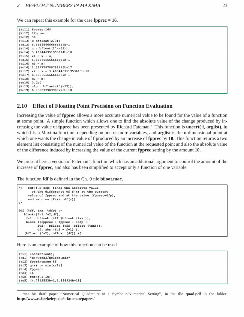
The functionfdf is defined in the Ch. 9 filebfloat.mac,
/ * fdf(f,x,dfp) finds the absolute valueof the difference of f(x) at the current
value of fpprec and at the value (fpprec+dfp),and returns [f(x), df(x)]
* /
fdf (%ff, %xx, %dfp) :=block([fv1,fv2,df],
fv1 : bfloat (%ff (bfloat (%xx))),block ([fpprec : fpprec + %dfp ],
fv2: bfloat (%ff (bfloat (%xx))),df: abs (fv2 - fv1) ),
[bfloat (fv2), bfloat (df)] )$
Here is an example of how this function can be used.
(%i1) load(bfloat);(%o1) "c:/work3/bfloat.mac"(%i2) fpprintprec:8$(%i3) g(x) := sin(x/2)$(%i4) fpprec;(%o4) 16(%i5) fdf(g,1,10);(%o5) [4.7942553b-1,1.834924b-18]
∗see his draft paper “Numerical Quadrature in a Symbolic/Numerical Setting”, in the filequad.pdf in the folder:http://www.cs.berkeley.edu/∼fateman/papers/

3 HIGH ACCURACY QUADRATURE WITH MAXIMA 24
(%i6) fdf(g,1,10),fpprec:30;(%o6) [4.7942553b-1,2.6824592b-33](%i7) fpprec;(%o7) 16
In the first example,fpprec is 16, and increasing the value to26 produces a change in the function value ofabout2× 10−18. In the second example,fpprec is 30, and increasing the value to40produces a change in thefunction value of about3× 10−33.
In the later section describing the “tanh-sinh” quadraturemethod, we will use this function for a heuristicestimate of the contribution of floating point errors to the approximate numerical value produced for an integralby that method.
3 High Accuracy Quadrature with Maxima
3.1 Using bromberg for High Accuracy Quadrature
A bigfloat version of the Romberg quadrature method is definedin Lisp code in the file.../share/numeric/brmbrg.lisp . You need to useload(brmbrg) or load("brmbrg.lisp") to beable to use the functionbromberg.
The use ofbromberg is identical to the use ofromberg (see the Maxima Manual entry forromberg ) exceptthatrombergtol (used for a possible return based on relative error) is replaced by the bigfloatbrombergtol witha default value of1.0b-4, andrombergabs (used for a possible return based on the absolute error) is replacedby the bigfloatbrombergabswhich has the default value0.0b0, andrombergit (which causes an return afterhalving the step size that many times) is replaced by the integerbrombergit which has the default value11,and finally,rombergmin (the minimum number of halving iterations) is replaced by the integerbrombergminwhich has the default value0.
If the function being integrated has a magnitude of order oneover the domain of integration, then an givenabsolute error is approximately equal to a the same relativeerror. We will testbromberg using the functionexp(x) over the domain[-1, 1], and use only the absolute error parameterbrombergabs, settingbrombergtolto 0.0b0so that the relative error test cannot be satisfied. Then the approximate value of the integral is returnedwhen the absolute value of the change in value from one halving iteration to the next is less than the bigfloatnumberbrombergabs.
We explore the use and behavior ofbromberg for the simple integral∫ 1
−1ex dx, binding a value accurate
to 42 digits totval, defining parameter values, callingbromberg first with fpprec equal to 30 together withbrombergabsset to1.0b-15and find an actual absolute error (compared withtval) of about7× 10−24.
(%i1) load(bfloat);(%o1) "c:/work3/bfloat.mac"(%i2) fpprintprec:8$(%i3) load(brmbrg);(%o3) "C:/Program Files (x86)/Maxima-sbcl-5.36.1/share /maxima/5.36.1/share/numeric/brmbrg.lisp"(%i4) [brombergtol,brombergabs,brombergit,brombergmi n,fpprec,fpprintprec];(%o4) [1.0b-4,0.0b0,11,0,16,8](%i5) integrate(exp(x),x,-1,1);(%o5) %e-%eˆ-1(%i6) tval : bfloat(%),fpprec:42;(%o6) 2.3504023b0(%i7) fpprec;(%o7) 16
3 HIGH ACCURACY QUADRATURE WITH MAXIMA 25
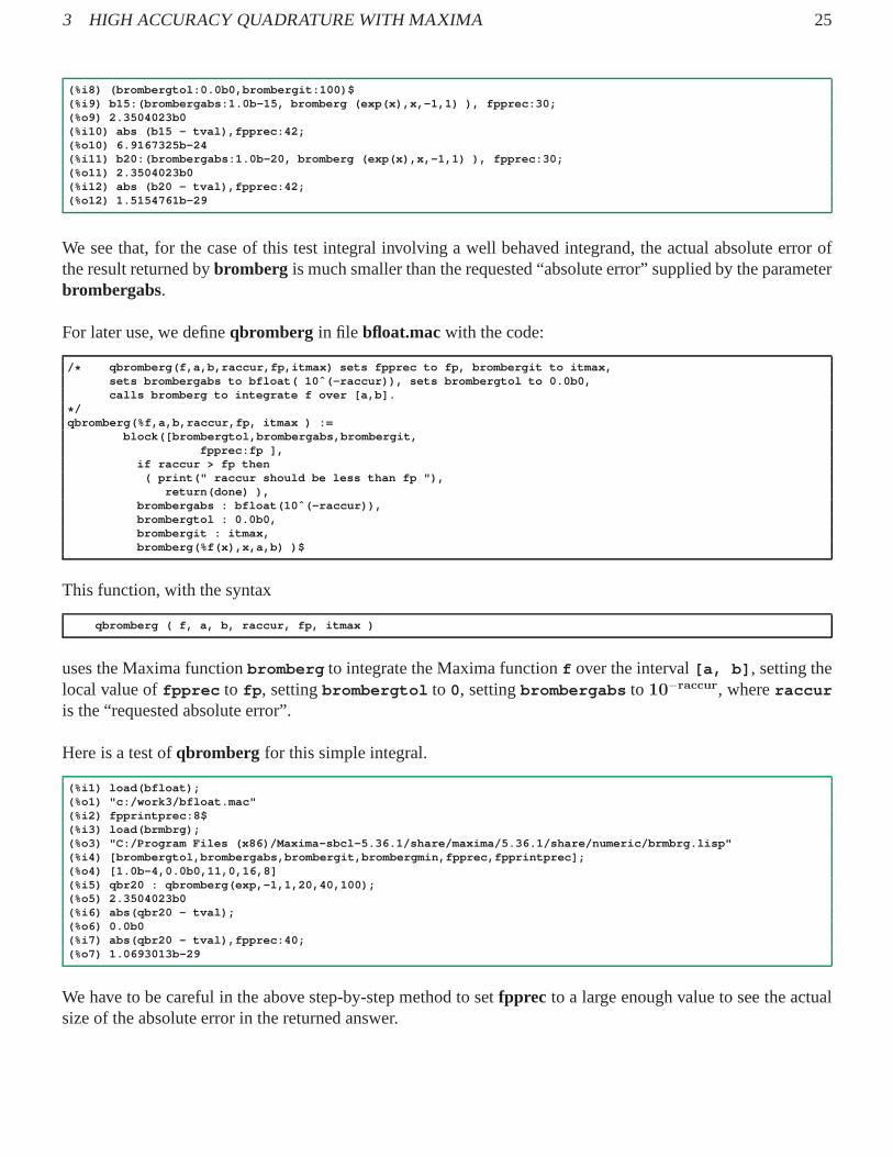
(%i8) (brombergtol:0.0b0,brombergit:100)$(%i9) b15:(brombergabs:1.0b-15, bromberg (exp(x),x,-1, 1) ), fpprec:30;(%o9) 2.3504023b0(%i10) abs (b15 - tval),fpprec:42;(%o10) 6.9167325b-24(%i11) b20:(brombergabs:1.0b-20, bromberg (exp(x),x,-1 ,1) ), fpprec:30;(%o11) 2.3504023b0(%i12) abs (b20 - tval),fpprec:42;(%o12) 1.5154761b-29
We see that, for the case of this test integral involving a well behaved integrand, the actual absolute error ofthe result returned bybromberg is much smaller than the requested “absolute error” supplied by the parameterbrombergabs.
For later use, we defineqbromberg in file bfloat.macwith the code:
/ * qbromberg(f,a,b,raccur,fp,itmax) sets fpprec to fp, brom bergit to itmax,sets brombergabs to bfloat( 10ˆ(-raccur)), sets brombergt ol to 0.0b0,calls bromberg to integrate f over [a,b].
* /qbromberg(%f,a,b,raccur,fp, itmax ) :=
block([brombergtol,brombergabs,brombergit,fpprec:fp ],
if raccur > fp then( print(" raccur should be less than fp "),
return(done) ),brombergabs : bfloat(10ˆ(-raccur)),brombergtol : 0.0b0,brombergit : itmax,bromberg(%f(x),x,a,b) )$
This function, with the syntax
qbromberg ( f, a, b, raccur, fp, itmax )
uses the Maxima functionbromberg to integrate the Maxima functionf over the interval[a, b] , setting thelocal value offpprec to fp , settingbrombergtol to 0, settingbrombergabs to 10−raccur, whereraccur
is the “requested absolute error”.
Here is a test ofqbromberg for this simple integral.
(%i1) load(bfloat);(%o1) "c:/work3/bfloat.mac"(%i2) fpprintprec:8$(%i3) load(brmbrg);(%o3) "C:/Program Files (x86)/Maxima-sbcl-5.36.1/share /maxima/5.36.1/share/numeric/brmbrg.lisp"(%i4) [brombergtol,brombergabs,brombergit,brombergmi n,fpprec,fpprintprec];(%o4) [1.0b-4,0.0b0,11,0,16,8](%i5) qbr20 : qbromberg(exp,-1,1,20,40,100);(%o5) 2.3504023b0(%i6) abs(qbr20 - tval);(%o6) 0.0b0(%i7) abs(qbr20 - tval),fpprec:40;(%o7) 1.0693013b-29
We have to be careful in the above step-by-step method to setfpprec to a large enough value to see the actualsize of the absolute error in the returned answer.

3 HIGH ACCURACY QUADRATURE WITH MAXIMA 26
Instead of the work involved in the above step by step method,it is more convenient to define a functionqbrlistwhich is passed a desiredfpprec as well as a list of requested absolute accuracy goals forbromberg. Thefunctionqbrlist then assumes a sufficiently accuratetval is globally defined, and proceeds through the listto calculate thebromberg value for each requested absolute accuracy, computes the actual absolute error inthe result, and prints a line containing (raccur, fpprec, value, value-error). Here is the code for such a function,defined inbfloat.mac:
/ * qbrlist(f,a,b,rplist,fp,itmax) assumes tval is globally defined, sets fpprec to fp,brombergit to itmax, computes bromberg integral of functio n f over [a,b] witheach raccur in rplist and computes absolute error of result.
* /qbrlist(%f,a,b,rplist,fp,itmax) :=
block([fpprec:fp,fpprintprec,brombergtol,brombergab s,brombergit,val,verr,raccur],if not listp(rplist) then (print("rplist # list"),return( done)),
brombergtol : 0.0b0,brombergit : itmax,fpprintprec:8,print(" raccur fpprec val verr "),print(" "),for raccur in rplist do
( brombergabs : bfloat(10ˆ(-raccur)),val: bromberg(%f(x),x,a,b),verr: abs(val - tval),print(" ",raccur," ",fp," ",val," ",verr) ) )$
and here is an example of use ofqbrlist in which the requested absolute errorraccur is set to three differentvalues supplied by the listrplist for each setting offpprec used. We use the “true” valuetval computedabove. Here is our test for three different values offpprec (the next to last arg):
(%i8) qbrlist(exp,-1,1,[10,15,17 ],20,100)$raccur fpprec val verr
10 20 2.3504023b0 4.5259436b-1415 20 2.3504023b0 1.3552527b-2017 20 2.3504023b0 1.3552527b-20
(%i9) qbrlist(exp,-1,1,[10,20,27 ],30,100)$raccur fpprec val verr
10 30 2.3504023b0 4.5259437b-1420 30 2.3504023b0 1.4988357b-2927 30 2.3504023b0 5.5220263b-30
(%i10) qbrlist(exp,-1,1,[10,20,30,35],40,100)$raccur fpprec val verr
10 40 2.3504023b0 4.5259437b-1420 40 2.3504023b0 1.0693013b-2930 40 2.3504023b0 1.1938614b-3935 40 2.3504023b0 1.1938614b-39
We see that withfpprec equal to40, increasingraccur from 30 to 35 results in no improvement in the actualabsolute error of the result.

3 HIGH ACCURACY QUADRATURE WITH MAXIMA 27
When bromberg Fails
One should not try to usebromberg for an integrand which has end point algebraic and/or logarithmicsingularities. Here is an example in which the integrand hasa logarithmic singularity at the lower end point:∫ 1
0
√t ln(t)dt. The integrate function has no problem with this integral. To illustrate the problem, we use
our homemade functionbromberg_abs(f,a,b,abserr) , defined inbfloat.mac .
(%i1) load(bfloat);(%o1) "c:/work3/bfloat.mac"(%i2) g(x):= sqrt(x) * log(x)$(%i3) i1 : integrate(g(t),t,0,1);(%o3) -4/9(%i4) fpprec : 20$(%i5) tval : bfloat(i1);(%o5) -4.4444444444444444445b-1(%i6) i18 : bromberg_abs(g,0,1,1.0b-18);log: encountered log(0).#0: g(x=0.0b0)#1: bromberg1(%f=g,a=0,b=1,n=2)#2: bromberg_abs(%g=g,%x1=0,%x2=1,%abserr=1.0b-18)(b float.mac line 286)
-- an error. To debug this try: debugmode(true);
The Maxima code forbromberg_abs , easier to follow than the Lisp code inbrmbrg.lisp , is based on theRomberg Method pseudo-code in Ch. 4 of the Seventh Ed. (2001)of Numerical Analysis by Burden andFaires.bromberg_abs(%g, %x1, %x2, %abserr) :=block([count,maxit:20,rval1,rval2 ],
%abserr : bfloat(%abserr),rval1 : bromberg1(%g,%x1,%x2,2),count :1,do (
rval2 : bromberg1(%g,%x1,%x2,count+3),if abs (rval2 - rval1) < %abserr then return(),count : count + 1,if count > maxit then (
print(" reached max number of iterations, maxit = ",maxit),return()),
rval1 : rval2 ),rval2)$
and the first call is tobromberg1(f,a,b,n) with n=2 . The code forbromberg1 is
bromberg1 (%f, a, b, n) :=block ([h, fxv, p,xL,fxL ],
local(R),a : bfloat(a),b : bfloat(b),h : (b - a),R[1,1] : h * (%f(a) + %f(b))/2.0b0,for i:2 thru n do (
p : 2ˆ(i-2),xL : makelist(a + (k - 0.5b0) * h, k ,1,p),fxL : map (%f, xL),/ * approximation from trapezoidal method * /R[2,1] : ( R[1,1] + h * apply ("+", fxL) )/ 2.0b0,/ * extrapolation * /for j:2 thru i do
R[2,j] : R[2,j-1] + (R[2,j-1] - R[1,j-1])/ bfloat(4ˆ(j-1) - 1),h : h/2.0b0,/ * update R[1,k] * /for j:1 thru i do R[1,j] : R[2,j]),
R[2,n])$
We then see that the first step taken bybromberg1(f,a,b,n) is to evaluate the given integrand at both of theendpoints of the given interval. Thus, this is more accurately called the Romberg End Point Method.
You can instead use the tanh-sinh quadrature method for thisintegral (see Sec. 3.3).
3 HIGH ACCURACY QUADRATURE WITH MAXIMA 28
3.2 A Double Exponential Quadrature Method fora ≤ x < ∞This method (H. Takahasi and M. Mori, 1974; see Sec 3.3) is effective for integrands which contain a factorwith some sort of exponential damping as the integration variable becomes large.
An integral of the form∫
∞
ag(y)dy can be converted into the integral
∫
∞
0f(x)dx by making the change of
variable of integrationy → x given byy = x+ a. Thenf(x) = g(x+ a).
The double exponential method used here then converts the integral∫
∞
0f(x)dx into the integral
∫
∞
−∞F(u)du
using a variable transformationx → u:
x(u) = exp(u− exp(−u)) (3.1)
and hence
F(u) = f(x(u))w(u), where w(u) =dx
du= exp(−exp(−u)) + x(u). (3.2)
You can confirm thatx(0) = exp(−1), w(0) = 2x(0) and thatx(−∞) = 0, x(∞) = ∞.
Because of the rapid decay of the integrand when the magnitude ofu is large, one can approximate the value ofthe infinite domainu integral by using a trapezoidal numerical approximation with step sizeh using a modestnumber (2N+ 1) of function evaluations.
I(h,N) ≃ hN∑
j=−N
F(uj) where uj = j h (3.3)
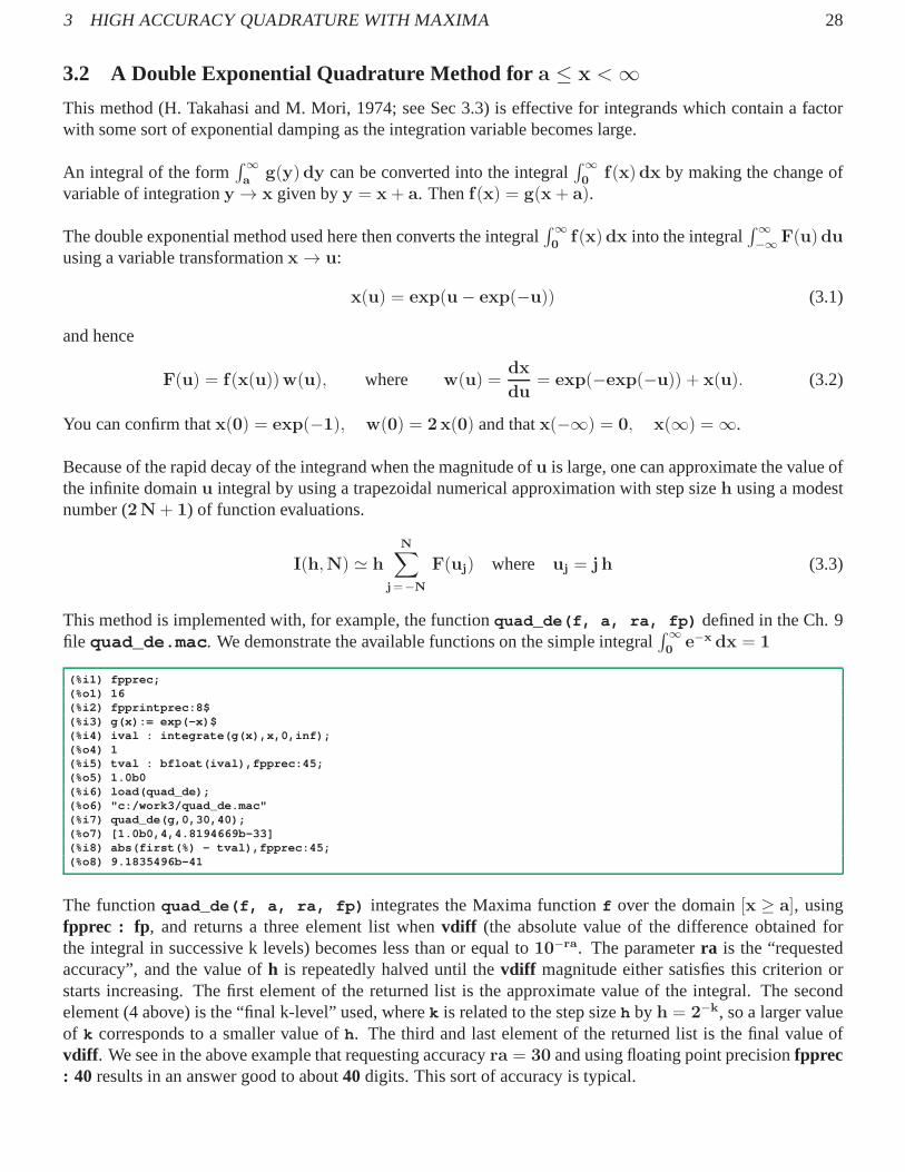
This method is implemented with, for example, the functionquad_de(f, a, ra, fp) defined in the Ch. 9file quad_de.mac . We demonstrate the available functions on the simple integral
∫
∞
0e−x dx = 1
(%i1) fpprec;(%o1) 16(%i2) fpprintprec:8$(%i3) g(x):= exp(-x)$(%i4) ival : integrate(g(x),x,0,inf);(%o4) 1(%i5) tval : bfloat(ival),fpprec:45;(%o5) 1.0b0(%i6) load(quad_de);(%o6) "c:/work3/quad_de.mac"(%i7) quad_de(g,0,30,40);(%o7) [1.0b0,4,4.8194669b-33](%i8) abs(first(%) - tval),fpprec:45;(%o8) 9.1835496b-41
The functionquad_de(f, a, ra, fp) integrates the Maxima functionf over the domain[x ≥ a], usingfpprec : fp , and returns a three element list whenvdiff (the absolute value of the difference obtained forthe integral in successive k levels) becomes less than or equal to 10−ra. The parameterra is the “requestedaccuracy”, and the value ofh is repeatedly halved until thevdiff magnitude either satisfies this criterion orstarts increasing. The first element of the returned list is the approximate value of the integral. The secondelement (4 above) is the “final k-level” used, wherek is related to the step sizeh byh = 2−k, so a larger valueof k corresponds to a smaller value ofh. The third and last element of the returned list is the final value ofvdiff . We see in the above example that requesting accuracyra = 30 and using floating point precisionfpprec: 40 results in an answer good to about40 digits. This sort of accuracy is typical.
3 HIGH ACCURACY QUADRATURE WITH MAXIMA 29
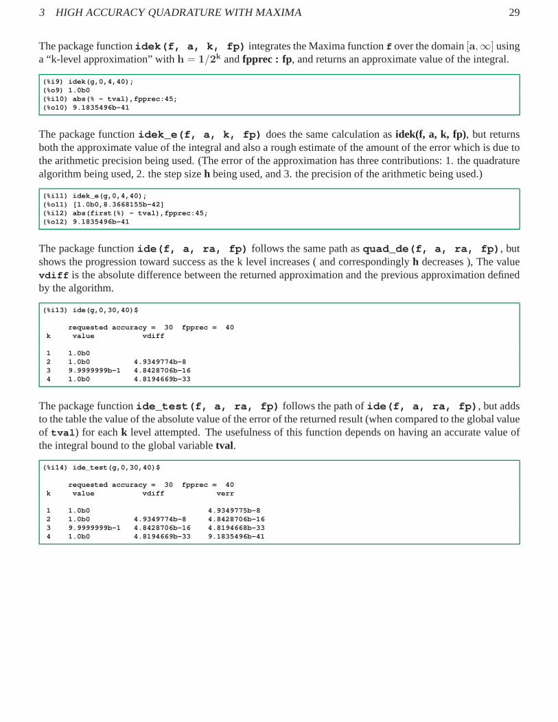
The package functionidek(f, a, k, fp) integrates the Maxima functionf over the domain[a,∞] usinga “k-level approximation” withh = 1/2k andfpprec : fp , and returns an approximate value of the integral.
(%i9) idek(g,0,4,40);(%o9) 1.0b0(%i10) abs(% - tval),fpprec:45;(%o10) 9.1835496b-41
The package functionidek_e(f, a, k, fp) does the same calculation asidek(f, a, k, fp), but returnsboth the approximate value of the integral and also a rough estimate of the amount of the error which is due tothe arithmetic precision being used. (The error of the approximation has three contributions: 1. the quadraturealgorithm being used, 2. the step sizeh being used, and 3. the precision of the arithmetic being used.)
(%i11) idek_e(g,0,4,40);(%o11) [1.0b0,8.3668155b-42](%i12) abs(first(%) - tval),fpprec:45;(%o12) 9.1835496b-41
The package functionide(f, a, ra, fp) follows the same path asquad_de(f, a, ra, fp) , butshows the progression toward success as the k level increases ( and correspondinglyh decreases ), The valuevdiff is the absolute difference between the returned approximation and the previous approximation definedby the algorithm.
(%i13) ide(g,0,30,40)$
requested accuracy = 30 fpprec = 40k value vdiff
1 1.0b02 1.0b0 4.9349774b-83 9.9999999b-1 4.8428706b-164 1.0b0 4.8194669b-33
The package functionide_test(f, a, ra, fp) follows the path ofide(f, a, ra, fp) , but addsto the table the value of the absolute value of the error of thereturned result (when compared to the global valueof tval ) for eachk level attempted. The usefulness of this function depends onhaving an accurate value ofthe integral bound to the global variabletval.
(%i14) ide_test(g,0,30,40)$
requested accuracy = 30 fpprec = 40k value vdiff verr
1 1.0b0 4.9349775b-82 1.0b0 4.9349774b-8 4.8428706b-163 9.9999999b-1 4.8428706b-16 4.8194668b-334 1.0b0 4.8194669b-33 9.1835496b-41

3 HIGH ACCURACY QUADRATURE WITH MAXIMA 30
Test Integral 1
Here we test this double exponential method code with the known integral
∫
∞
0
e−t
√tdt =
√π (3.4)
(%i15) g(x):= exp(-x)/sqrt(x)$(%i16) integrate(g(t),t,0,inf);(%o16) sqrt(%pi)(%i17) tval : bfloat(%),fpprec:45;(%o17) 1.7724538b0(%i18) quad_de(g,0,30,40);(%o18) [1.7724538b0,4,1.0443243b-34](%i19) abs(first(%) - tval),fpprec:45;(%o19) 1.8860005b-40(%i20) idek_e(g,0,4,40);(%o20) [1.7724538b0,2.7054206b-41]
Again we see that the combinationra = 30, fp = 40 leads to an answer good to about40 accurate digits .
Test Integral 2
Our second known integral is∫
∞
0
e−t2/2 dt =√
π/2 (3.5)
(%i21) g(x) := exp(-xˆ2/2)$(%i22) tval : bfloat(sqrt(%pi/2)),fpprec:45$(%i23) quad_de(g,0,30,40);(%o23) [1.2533141b0,5,1.099771b-31](%i24) abs(first(%) - tval),fpprec:45;(%o24) 2.1838045b-40(%i25) idek_e(g,0,5,40);(%o25) [1.2533141b0,1.3009564b-41]
Test Integral 3
Our third test integral is∫
∞
0
e−t cos t dt = 1/2 (3.6)
(%i26) g(x) := exp(-x) * cos(x)$(%i27) integrate(g(x),x,0,inf);(%o27) 1/2(%i28) tval : bfloat(%),fpprec:45$(%i29) quad_de(g,0,30,40);(%o29) [5.0b-1,5,1.7998243b-33](%i30) abs(first(%) - tval),fpprec:45;(%o30) 9.1835496b-41(%i31) idek_e(g,0,5,40);(%o31) [5.0b-1,9.8517724b-42]

3 HIGH ACCURACY QUADRATURE WITH MAXIMA 31
3.3 The tanh-sinh Quadrature Method fora ≤ x ≤ b
H. Takahasi and M. Mori (1974: see references at the end of this section) presented an efficient method forthe numerical integration of the integral of a function overa finite domain. This method is known under thenames “tanh-sinh method” and “double exponential method”.This method can handle integrands which havealgebraic and logarithmic end point singularities, and is well suited for use with high accuracy work.
Quoting (loosely) David Bailey’s (see references below) slide presentations on this subject:
The tanh-sinh quadrature method can accurately handle all “reasonable functions”, even thosewith “blow-up singularities” or vertical slopes at the end points of the integration interval. In manycases, reducing the step size h by half doubles the number of correct digits in the result returned(“quadratic convergence”).
An integral of the form∫ b
ag(y)dy can be converted into the integral
∫ 1
−1f(x)dx by making the change
of variable of integrationy → x given by y = αx+ β with α = (b− a)/2 and β = (a+ b)/2. Thenf(x) = αg(αx + β).
The tanh-sinh method introduces a change of variablesx → u which implies
∫ 1
−1
f(x)dx =
∫
∞
−∞
F(u)du. (3.7)
The change of variables is expressed by
x(u) = tanh(π
2sinhu
)
(3.8)
and you can confirm that
u = 0 ⇒ x = 0, u → −∞ ⇒ x → −1,u → ∞ ⇒ x → 1 (3.9)
We also havex(−u) = −x(u).
The “weight”w(u) = dx(u)/du is
w(u) =π
2coshu
cosh2(
π
2sinhu
) (3.10)
with the propertyw(−u) = w(u), in terms of whichF(u) = f(x(u)w(u). Moreover,F(u) has “doubleexponential behavior” of the form
F(u) ≈ exp(
−π
2exp( |u | )
)
for u → ±∞. (3.11)
Because of the rapid decay of the integrand when the magnitude ofu is large, one can approximate the valueof the infinite domain integral by using a trapezoidal numerical approximation with step sizeh using a modestnumber (2N+ 1) of function evaluations.
I(h,N) ≃ hN∑
j=−N
F(uj) where uj = j h (3.12)

3 HIGH ACCURACY QUADRATURE WITH MAXIMA 32
This method is implemented with, for example, the functionquad_ts (f, a, b, ra, fp ) defined inthe Ch. 9 filequad_ts.mac , and we will illustrate the available package functions using the simple integral∫ 1
−1ex dx.
The package functionquad_ts (f, a, b, ra, fp ) is the most useful workhorse for routine use, anduses the tanh-sinh method to integrate the Maxima functionf over the finite interval[a, b] , stopping whenthe absolute value of the difference(Ik − Ik−1) is less than10−ra (ra is the “requested accuracy” for theresult), usingfp digit precision arithmetic (fpprec set tofp , andbfloat being used to enforce this arithmeticprecision). This function returns the list[ approx-value, k-level-used, abs(vdiff) ] , where the last element should be smaller than10−ra .
(%i1) fpprec;(%o1) 16(%i2) fpprintprec:8$(%i3) tval : bfloat( integrate( exp(x),x,-1,1 )),fpprec:4 5;(%o3) 2.3504023b0(%i4) load(quad_ts);
_kmax% = 8 _epsfac% = 2(%o4) "c:/work3/quad_ts.mac"(%i5) bfprint(tval,45)$
number of digits = 452.35040238728760291376476370119120163031143596b0
(%i6) quad_ts(exp,-1,1,30,40);construct _yw%[kk,fpprec] array for kk =
8 and fpprec = 40 ...working...(%o6) [2.3504023b0,5,0.0b0](%i7) abs(first(%) - tval),fpprec:45;(%o7) 2.719612b-40
A value of the integral accurate to about 45 digits is bound tothe symboltval. The package functionbfprint(bf, fpp) allows controlled printing offpp digits of the “true value”tval to the screen. We thencompare the approximate quadrature result with this “true value”. The packagequad_ts.mac defines twoglobal parameters._kmax% is the maximum “k-level” possible (the defined default is 8, which means theminimum step size for the transformed “u-integral” isdu = h = 1/28 = 1/256. The actual “k-level” neededto return a result with the requested accuracyra is the integer in the second element of the returned list. Theglobal parameter_epsfac% (default value2) is used to decide how many(y, w) numbers to pre-compute(see below).
We see that a “k-level” approximation withk = 5 andh = 1/25 = 1/32 returned an answer with an actualaccuracy of about 40 correct digits (whenra = 30 andfp = 40).
The first time 40 digit precision arithmetic is called for, a set of (y, w) numbers are calculated and stored inan array which we call_yw%[8, 40] . They(u) values will later be converted tox(u) numbers using highprecision, and the original integrand functionf(x(u)) is also calculated at high precision. Thew(u) numbersare what we call “weights”, and are needed for the numbersF(u) = f(x(u))w(u) used in the trapezoidal ruleevaluation. The package precomputes pairs(y, w) for larger and larger values ofu until the magnitude of theweightw becomes less thaneps , whereeps = 10−np, wheren is the global parameter_epsfac% (default2)andp is the requested floating point precisionfp .
Once the set of40-digit precision(y, w) numbers have been “pre-computed”, they can be used for theevaluation of any similar precision integrals later, sincethese numbers are independent of the actual functionbeing integrated, but depend only on the nature of the tanh-sinh transformation being used.

3 HIGH ACCURACY QUADRATURE WITH MAXIMA 33
The package functionqtsk(f, a, b, k, fp) (note: argk replacesra ) integrates the Maxima functionf over the domain[a,b] using a “k-level approximation” withh = 1/2k andfpprec : fp .
(%i8) qtsk(exp,-1,1,5,40);(%o8) 2.3504023b0(%i9) abs(% - tval),fpprec:45;(%o9) 2.719612b-40
A heuristic value of the error contribution due to the arithmetic precision being used (which is separate fromthe error contribution due to the nature of the algorithm andthe step size being used) can be found by usingthe package functionqtsk_e(f, a, b, k, fp); . The first element of the returned list is the value of theintegral, the second element of the returned list is a rough estimate of the contribution of the floating pointarithmetic precision being used to the error of the returnedanswer.
(%i10) qtsk_e(exp,-1,1,5,40);(%o10) [2.3504023b0,2.0614559b-94](%i11) abs(first(%) - tval),fpprec:45;(%o11) 2.719612b-40
The very small estimate of the arithmetic precision contribution (two parts in1094) to the error of the an-swer is due to the high precision being used to convert from the pre-computedy to the needed abcissax viax : bfloat(1− y) and the subsequent evaluationf(x). The precision being used depends on the size of thesmallesty number, which will always be that appearing in the last element of the hashed array_yw%[8, 40] .
(%i12) last(_yw%[8,40]);(%o12) [4.7024891b-83,8.9481574b-81]
(In Eq. (3.12) we have separated out the(u = 0, x = 0)term, and used the symmetry propertiesx(−u) = −x(u),andw(−u) = w(u) to write the remainder as a sum over positive values ofu (and hence positive values ofx)so only the largeu values ofy(u) need to be pre-computed).
We see that the smallesty number is about5× 10−83 and if we subtract this from1 we will get 1 unless weuse a very high precision. It turns out that asu approaches plus infinity,x (as used here) approachesb (whichis 1 in our example) from values less thanb. Since a principal virtue of the tanh-sinh method is its ability tohandle integrands which “blow up” at the limits of integration, we need to make sure we stay away (even ifonly a little) from those end limits.
We can see the precision with which the arithmetic is being carried out in this crucial step by using thefpxy(fp)function
(%i13) fpxy(40)$the last y value = 4.7024891b-83the fpprec being used for x and f(x) is 93
and this explains the small number returned (as the second element) byqtsk_e(exp, -1, 1, 5, 40); .
The package functionqts(f, a, b, ra, fp) follows the same path asquad_ts(f, a, b, ra, fp) ,but shows the progression toward success as thek level increases ( andh decreases ):
(%i14) qts(exp,-1,1,30,40)$ra = 30 fpprec = 40k newval vdiff
1 2.350282b02 2.3504023b0 1.2031242b-43 2.3504023b0 8.136103b-114 2.3504023b0 1.9907055b-235 2.3504023b0 0.0b0

3 HIGH ACCURACY QUADRATURE WITH MAXIMA 34
The package functionqts_test(f, a, b, ra, fp) follows the path ofqts(f, a, b, ra, fp) ,but adds to the table the value of the absolute error of the approximate result for eachk level attempted. Theuse of this function depends on an accurate value of the integral being bound to the global variabletval.
(%i15) qts_test(exp,-1,1,30,40)$ra = 30 fpprec = 40
k value vdiff verr1 2.350282b0 1.2031234b-42 2.3504023b0 1.2031242b-4 8.136103b-113 2.3504023b0 8.136103b-11 1.9907055b-234 2.3504023b0 1.9907055b-23 2.7550648b-405 2.3504023b0 0.0b0 2.7550648b-40
Test Integral 1
Here we test this tanh-sinh method code with the known integral which confoundedbromberg_abs in Sec.3.1 :
∫ 1
0
√t ln(t)dt = −4/9 (3.13)
(%i16) g(x):= sqrt(x) * log(x)$(%i17) tval : bfloat(integrate(g(t),t,0,1)),fpprec:45;(%o17) -4.4444444b-1(%i18) quad_ts(g,0,1,30,40);(%o18) [-4.4444444b-1,5,3.4438311b-41](%i19) abs(first(%) - tval),fpprec:45;(%o19) 4.4642216b-41(%i20) qtsk_e(g,0,1,5,40);(%o20) [-4.4444444b-1,7.9678502b-44]
Requesting thirty digit accuracy with forty digit arithmetic returns a value for this integral which has about fortycorrect digits. Note that “vdiff” (the third and last element of the list returned byquad_ts(g,0,1,30,40) )is approximately the same as the actual absolute error.
Test Integral 2
Consider the integral∫ 1
0
arctan(√2+ t2)
(1+ t2)√2+ t2
dt = 5π2/96. (3.14)
(%i21) g(x):= atan(sqrt(2+xˆ2))/(sqrt(2+xˆ2) * (1+xˆ2))$(%i22) integrate(g(t),t,0,1);(%o22) ’integrate(atan(sqrt(tˆ2+2))/((tˆ2+1) * sqrt(tˆ2+2)),t,0,1)(%i23) quad_qags(g(t),t,0,1);(%o23) [0.5140419,5.7070115e-15,21,0](%i24) float(5 * %piˆ2/96);(%o24) 0.5140419(%i25) tval: bfloat(5 * %piˆ2/96),fpprec:45;(%o25) 5.1404189b-1(%i26) quad_ts(g,0,1,30,40);(%o26) [5.1404189b-1,5,1.5634993b-36](%i27) abs(first(%) - tval),fpprec:45;(%o27) 7.3300521b-41(%i28) qtsk_e(g,0,1,5,40);(%o28) [5.1404189b-1,1.3887835b-43]
3 HIGH ACCURACY QUADRATURE WITH MAXIMA 35
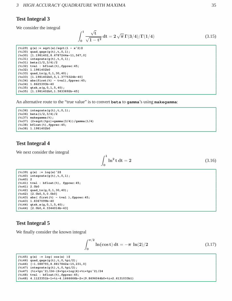
Test Integral 3
We consider the integral∫ 1
0
√t√
1− t2dt = 2
√πΓ(3/4)/Γ(1/4) (3.15)
(%i29) g(x):= sqrt(x)/sqrt(1 - xˆ2)$(%i30) quad_qags(g(t),t,0,1);(%o30) [1.1981402,8.6787244e-11,567,0](%i31) integrate(g(t),t,0,1);(%o31) beta(1/2,3/4)/2(%i32) tval : bfloat(%),fpprec:45;(%o32) 1.1981402b0(%i33) quad_ts(g,0,1,30,40);(%o33) [1.1981402b0,5,1.3775324b-40](%i34) abs(first(%) - tval),fpprec:45;(%o34) 1.8625393b-40(%i35) qtsk_e(g,0,1,5,40);(%o35) [1.1981402b0,1.5833892b-45]
An alternative route to the “true value” is to convertbeta to gamma’s usingmakegamma:
(%i36) integrate(g(t),t,0,1);(%o36) beta(1/2,3/4)/2(%i37) makegamma(%);(%o37) (2 * sqrt(%pi) * gamma(3/4))/gamma(1/4)(%i38) bfloat(%),fpprec:45;(%o38) 1.1981402b0
Test Integral 4
We next consider the integral∫ 1
0
ln2 t dt = 2 (3.16)
(%i39) g(x) := log(x)ˆ2$(%i40) integrate(g(t),t,0,1);(%o40) 2(%i41) tval : bfloat(%), fpprec:45;(%o41) 2.0b0(%i42) quad_ts(g,0,1,30,40);(%o42) [2.0b0,5,0.0b0](%i43) abs( first(%) - tval ),fpprec:45;(%o43) 1.8367099b-40(%i44) qtsk_e(g,0,1,5,40);(%o44) [2.0b0,4.3344016b-43]
Test Integral 5
We finally consider the known integral∫
π/2
0
ln(cos t)dt = −π ln(2)/2 (3.17)
(%i45) g(x) := log( cos(x) )$(%i46) quad_qags(g(t),t,0,%pi/2);(%o46) [-1.088793,8.8817842e-15,231,0](%i47) integrate(g(t),t,0,%pi/2);(%o47) (%i * %piˆ2)/24-(6 * %pi * log(4)+%i * %piˆ2)/24(%i48) tval : bfloat(%),fpprec:45;(%o48) 4.1123351b-1 * %i-4.1666666b-2 * (9.8696044b0 * %i+2.6131033b1)

3 HIGH ACCURACY QUADRATURE WITH MAXIMA 36
(%i49) rectform(%);(%o49) (-6.9388939b-18 * %i)-1.088793b0(%i50) float(-%pi * log(2)/2);(%o50) -1.088793(%i51) tval : bfloat(-%pi * log(2)/2),fpprec:45;(%o51) -1.088793b0(%i52) quad_ts(g,0,%pi/2,30,40);(%o52) [1.2979374b-80 * %i-1.088793b0,5,9.1835496b-41](%i53) ans: realpart( first(%) ),fpprec:45;(%o53) -1.088793b0(%i54) abs(ans - tval),fpprec:45;(%o54) 1.9661688b-40(%i55) qtsk_e(g,0,%pi/2,5,40);(%o55) [1.2979374b-80 * %i-1.088793b0,1.2858613b-42]
We see that the tanh-sinh result includes a tiny imaginary part due to bigfloat errors, and taking the real partproduces an answer good to about 40 digits (usingra = 30, fp = 40 ).
References for the tanh-sinh Quadrature Method
This method was initially described in the articleDouble Exponential Formulas for Numerical Integration, by HidetosiTakahasi and Masatake Mori, in the journal Publications of the Research Institute for Mathematical Sciences ( Publ.RIMS), vol.9, Number 3, (1974), 721-741, Kyoto University,Japan. A recent summary by the second author isDiscoveryof the Double Exponential Transformation and Its Developments, by Masatake Mori, Publ. RIMS, vol.41, Number 4,(2005), 897-935. Both of the above articles can be downloaded from the Project Euclid RIMS webpage
http://projecteuclid.org/DPubS?service=UI&version=1.0&verb=Display&page=past &handle=euclid.prims
A good summary of implementation ideas can be found in the report Tanh-Sinh High-Precision Quadrature, by DavidH. Bailey, Jan. 2006, LBNL-60519, which can be downloaded from the webpage
http://crd.lbl.gov/˜dhbailey/dhbpapers/
Further Improvements for the tanh-sinh Quadrature Method
The code provided in the filequad_ts.mac has been lightly tested, and should be used with caution.
No proper investigation has been made of the efficiency of choosing to use a floating point precision (for all terms of thesum) based on the small size of the smallesty value.
No attempt has been made to translate into Lisp and compile the code to make timing trials for comparison purposes.
These (and other) refinements are left to the initiative of the hypothetical alert reader of limitless dedication (HAROLD).
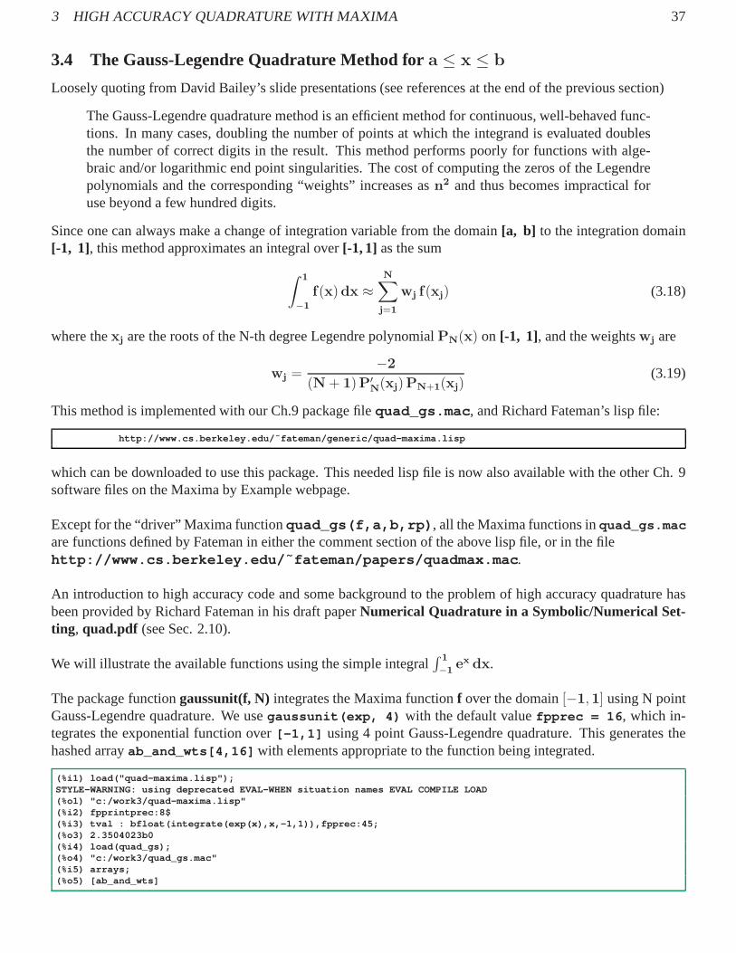
3 HIGH ACCURACY QUADRATURE WITH MAXIMA 37
3.4 The Gauss-Legendre Quadrature Method fora ≤ x ≤ b
Loosely quoting from David Bailey’s slide presentations (see references at the end of the previous section)
The Gauss-Legendre quadrature method is an efficient methodfor continuous, well-behaved func-tions. In many cases, doubling the number of points at which the integrand is evaluated doublesthe number of correct digits in the result. This method performs poorly for functions with alge-braic and/or logarithmic end point singularities. The costof computing the zeros of the Legendrepolynomials and the corresponding “weights” increases asn2 and thus becomes impractical foruse beyond a few hundred digits.
Since one can always make a change of integration variable from the domain[a, b] to the integration domain[-1, 1], this method approximates an integral over[-1, 1] as the sum
∫ 1
−1
f(x)dx ≈N∑
j=1
wj f(xj) (3.18)
where thexj are the roots of the N-th degree Legendre polynomialPN(x) on [-1, 1], and the weightswj are
wj =−2
(N+ 1)P′
N(xj)PN+1(xj)(3.19)
This method is implemented with our Ch.9 package filequad_gs.mac , and Richard Fateman’s lisp file:
http://www.cs.berkeley.edu/˜fateman/generic/quad-ma xima.lisp
which can be downloaded to use this package. This needed lispfile is now also available with the other Ch. 9software files on the Maxima by Example webpage.
Except for the “driver” Maxima functionquad_gs(f,a,b,rp) , all the Maxima functions inquad_gs.mac
are functions defined by Fateman in either the comment section of the above lisp file, or in the filehttp://www.cs.berkeley.edu/˜fateman/papers/quadmax. mac.
An introduction to high accuracy code and some background tothe problem of high accuracy quadrature hasbeen provided by Richard Fateman in his draft paperNumerical Quadrature in a Symbolic/Numerical Set-ting, quad.pdf (see Sec. 2.10).
We will illustrate the available functions using the simpleintegral∫ 1
−1ex dx.
The package functiongaussunit(f, N)integrates the Maxima functionf over the domain[−1, 1] using N pointGauss-Legendre quadrature. We usegaussunit(exp, 4) with the default valuefpprec = 16 , which in-tegrates the exponential function over[-1,1] using 4 point Gauss-Legendre quadrature. This generates thehashed arrayab_and_wts[4,16] with elements appropriate to the function being integrated.
(%i1) load("quad-maxima.lisp");STYLE-WARNING: using deprecated EVAL-WHEN situation name s EVAL COMPILE LOAD(%o1) "c:/work3/quad-maxima.lisp"(%i2) fpprintprec:8$(%i3) tval : bfloat(integrate(exp(x),x,-1,1)),fpprec:4 5;(%o3) 2.3504023b0(%i4) load(quad_gs);(%o4) "c:/work3/quad_gs.mac"(%i5) arrays;(%o5) [ab_and_wts]

3 HIGH ACCURACY QUADRATURE WITH MAXIMA 38
(%i6) arrayinfo(ab_and_wts);(%o6) [hashed,2](%i7) gaussunit(exp,4);(%o7) 2.350402b0(%i8) abs(% - tval),fpprec:45;(%o8) 2.9513122b-7(%i9) fpprec;(%o9) 16(%i10) arrayinfo(ab_and_wts);(%o10) [hashed,2,[4,16]](%i11) first( ab_and_wts[4, 16] );(%o11) [8.6113631b-1,3.3998104b-1](%i12) second( ab_and_wts[4, 16] );(%o12) [3.4785484b-1,6.5214515b-1](%i13) lp4 : legenp(4,x);(%o13) (35 * xˆ4)/8-(15 * xˆ2)/4+3/8(%i14) float(solve(lp4));(%o14) [x = -0.86113631,x = 0.86113631,x = -0.33998104,x = 0 .33998104](%i15) ab_and_wts[4,16];(%o15) [[8.6113631b-1,3.3998104b-1],[3.4785484b-1,6. 5214515b-1]]
With the default value offpprec = 16 and using only four integrand evaluation points (with approximatevalues given by%o14), the error is about 2 parts in107. Thefirst element %o11of the two index hashed arrayab_and_wts[4,16] is a list of thepositivezeros of the fourth order Legendre polynomialP4(x) ( calculatedwith 16 digit arithmetic,fpprec = 16).
That fourth order Legendre polynomialP4(x) can be displayed with this package usinglegenp(4, x) .Usingsolvewe see that the roots for negativex are simply the the positive roots with a minus sign, so the al-gorithm used makes use of this symmetry and keeps track of only the positive roots, as seen in the output%o11.
We can verify that the list of (positive) roots%o11returned is correct to within the global floating point precision(we do this two different ways):
(%i16) lfp4(x) := legenp(4,x)$(%i17) map(’lfp4,%o11);(%o17) [0.0b0,-3.4694469b-18](%i18) map( lambda([z], legenp (4, z)),%o11 );(%o18) [0.0b0,-3.4694469b-18]
Thesecond elementof ab_and_wts[4,16] is a list of the weights which are associated with the positiveroots (the negative roots have the same weights), with ordercorresponding to the order of the returned positiveroots.
The package functiongaussunit_e(f, N) does the same job asgaussunit(f, N) , but returns arough estimate of the amount contributed to the error by the floating point precision used (as the second elementof the returned list:
(%i19) gaussunit_e(exp,4);(%o19) [2.350402b0,1.2761299b-17](%i20) arrayinfo(ab_and_wts);(%o20) [hashed,2,[4,16]]
We see that the error attributable to the floating point precision used is insignificant compared to the error dueto the low number of integrand evaluation points for this example.
An arbitrary finite integration interval is allowed with the functionsgaussab(f, a, b, N) andgaussab_e(f, a, b, N) which useN point Gauss-Legendre quadrature over the interval[a,b], with thelatter function being the analog ofgaussunit_e(f, N) .
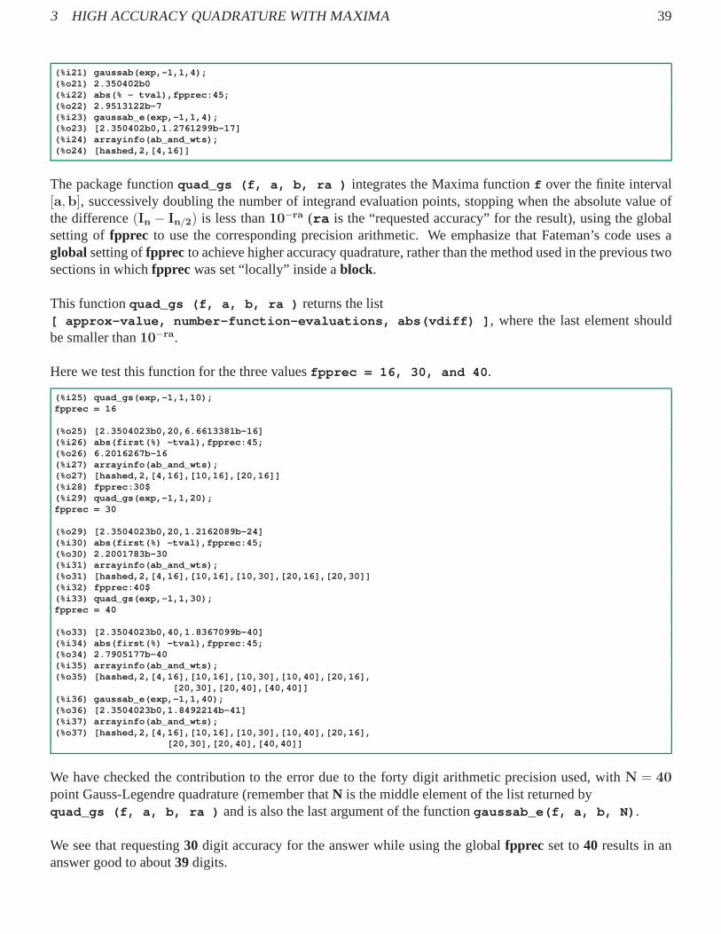
3 HIGH ACCURACY QUADRATURE WITH MAXIMA 39
(%i21) gaussab(exp,-1,1,4);(%o21) 2.350402b0(%i22) abs(% - tval),fpprec:45;(%o22) 2.9513122b-7(%i23) gaussab_e(exp,-1,1,4);(%o23) [2.350402b0,1.2761299b-17](%i24) arrayinfo(ab_and_wts);(%o24) [hashed,2,[4,16]]
The package functionquad_gs (f, a, b, ra ) integrates the Maxima functionf over the finite interval[a,b], successively doubling the number of integrand evaluationpoints, stopping when the absolute value ofthe difference(In − In/2) is less than10−ra (ra is the “requested accuracy” for the result), using the globalsetting offpprec to use the corresponding precision arithmetic. We emphasize that Fateman’s code uses aglobal setting offpprec to achieve higher accuracy quadrature, rather than the method used in the previous twosections in whichfpprec was set “locally” inside ablock.
This functionquad_gs (f, a, b, ra ) returns the list[ approx-value, number-function-evaluations, abs(vdiff ) ] , where the last element shouldbe smaller than10−ra.
Here we test this function for the three valuesfpprec = 16, 30, and 40 .
(%i25) quad_gs(exp,-1,1,10);fpprec = 16
(%o25) [2.3504023b0,20,6.6613381b-16](%i26) abs(first(%) -tval),fpprec:45;(%o26) 6.2016267b-16(%i27) arrayinfo(ab_and_wts);(%o27) [hashed,2,[4,16],[10,16],[20,16]](%i28) fpprec:30$(%i29) quad_gs(exp,-1,1,20);fpprec = 30
(%o29) [2.3504023b0,20,1.2162089b-24](%i30) abs(first(%) -tval),fpprec:45;(%o30) 2.2001783b-30(%i31) arrayinfo(ab_and_wts);(%o31) [hashed,2,[4,16],[10,16],[10,30],[20,16],[20, 30]](%i32) fpprec:40$(%i33) quad_gs(exp,-1,1,30);fpprec = 40
(%o33) [2.3504023b0,40,1.8367099b-40](%i34) abs(first(%) -tval),fpprec:45;(%o34) 2.7905177b-40(%i35) arrayinfo(ab_and_wts);(%o35) [hashed,2,[4,16],[10,16],[10,30],[10,40],[20, 16],
[20,30],[20,40],[40,40]](%i36) gaussab_e(exp,-1,1,40);(%o36) [2.3504023b0,1.8492214b-41](%i37) arrayinfo(ab_and_wts);(%o37) [hashed,2,[4,16],[10,16],[10,30],[10,40],[20, 16],
[20,30],[20,40],[40,40]]
We have checked the contribution to the error due to the fortydigit arithmetic precision used, withN = 40point Gauss-Legendre quadrature (remember thatN is the middle element of the list returned byquad_gs (f, a, b, ra ) and is also the last argument of the functiongaussab_e(f, a, b, N) .
We see that requesting30 digit accuracy for the answer while using the globalfpprec set to40 results in ananswer good to about39 digits.
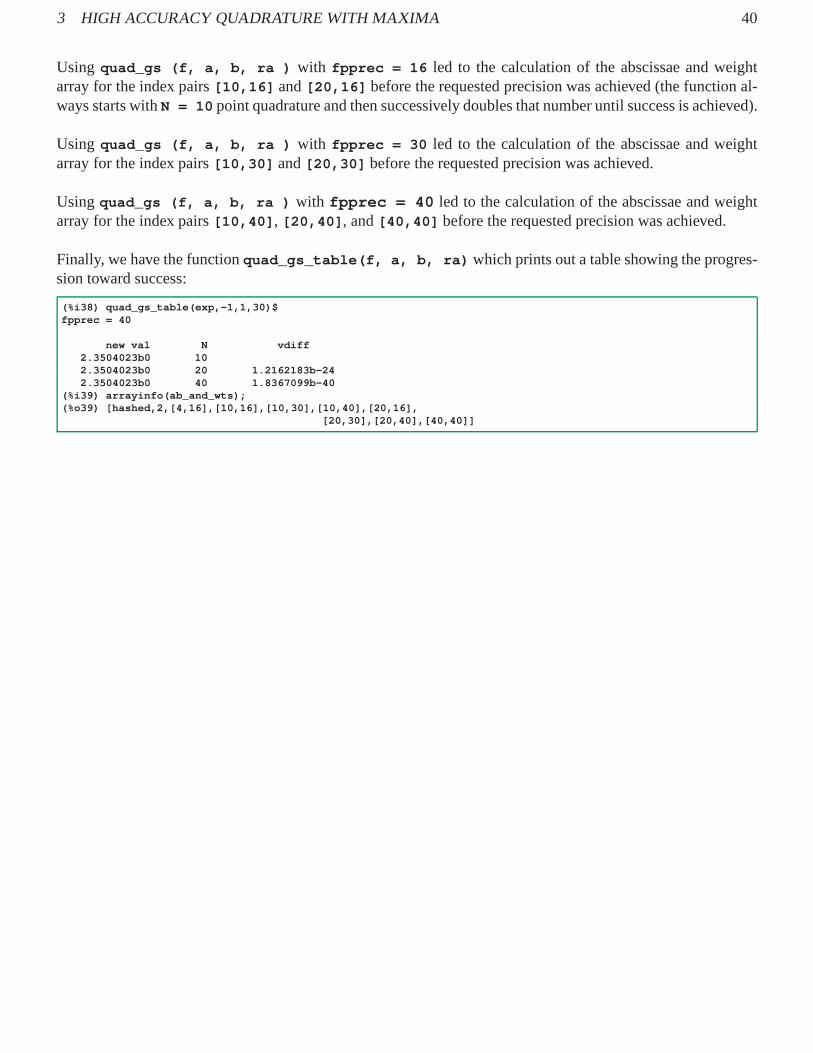
3 HIGH ACCURACY QUADRATURE WITH MAXIMA 40
Using quad_gs (f, a, b, ra ) with fpprec = 16 led to the calculation of the abscissae and weightarray for the index pairs[10,16] and[20,16] before the requested precision was achieved (the function al-ways starts withN = 10 point quadrature and then successively doubles that numberuntil success is achieved).
Using quad_gs (f, a, b, ra ) with fpprec = 30 led to the calculation of the abscissae and weightarray for the index pairs[10,30] and[20,30] before the requested precision was achieved.
Using quad_gs (f, a, b, ra ) with fpprec = 40 led to the calculation of the abscissae and weightarray for the index pairs[10,40] , [20,40] , and[40,40] before the requested precision was achieved.
Finally, we have the functionquad_gs_table(f, a, b, ra) which prints out a table showing the progres-sion toward success:
(%i38) quad_gs_table(exp,-1,1,30)$fpprec = 40
new val N vdiff2.3504023b0 102.3504023b0 20 1.2162183b-242.3504023b0 40 1.8367099b-40
(%i39) arrayinfo(ab_and_wts);(%o39) [hashed,2,[4,16],[10,16],[10,30],[10,40],[20, 16],
[20,30],[20,40],[40,40]]