Rigorous data-driven computation of spectral properties of

Koopman operators for dynamical systems

Matthew J. Colbrook∗ Alex Townsend†

December 1, 2021

Abstract

Koopman operators are infinite-dimensional operators that globally linearize nonlinear dynamicalsystems, making their spectral information useful for understanding dynamics. However, Koopmanoperators can have continuous spectra and infinite-dimensional invariant subspaces, making comput-ing their spectral information a considerable challenge. This paper describes data-driven algorithmswith rigorous convergence guarantees for computing spectral information of Koopman operators fromtrajectory data. We introduce residual dynamic mode decomposition (ResDMD), which provides thefirst scheme for computing the spectra and pseudospectra of general Koopman operators from snap-shot data without spectral pollution. Using the resolvent operator and ResDMD, we also computesmoothed approximations of spectral measures associated with measure-preserving dynamical sys-tems. We prove explicit convergence theorems for our algorithms, which can achieve high-order con-vergence even for chaotic systems, when computing the density of the continuous spectrum and thediscrete spectrum. We demonstrate our algorithms on the tent map, Gauss iterated map, nonlinearpendulum, double pendulum, Lorenz system, and an 11-dimensional extended Lorenz system. Fi-nally, we provide kernelized variants of our algorithms for dynamical systems with a high-dimensionalstate-space. This allows us to compute the spectral measure associated with the dynamics of a pro-tein molecule that has a 20,046-dimensional state-space, and compute nonlinear Koopman modeswith error bounds for turbulent flow past aerofoils with Reynolds number > 105 that has a 295,122-dimensional state-space.

Keywords: Dynamical systems, Koopman operator, Data-driven discovery, Dynamic mode decom-position, Spectral theory

AMS subject classifications: 37M10, 65P99, 65F99, 65T99, 37A30, 47A10, 47B33, 37N10, 37N25

1 Introduction

Dynamical systems are a mathematical description of time-dependent states or quantities that char-acterize evolving processes in classical mechanics, electrical circuits, fluid flows, climatology, finance,neuroscience, epidemiology, and many other fields. Throughout the paper, we consider autonomous dy-namical systems whose state evolves over a state-space Ω ⊆ Rd in discrete time-steps according to afunction F : Ω→ Ω. In other words, we consider dynamical systems of the form

xxxn+1 = F (xxxn), n ≥ 0, (1.1)

where xxx0 is a given initial condition. Such a dynamical system forms a trajectory of iterates xxx0,xxx1,xxx2, . . . ,in Ω. We are interested in answering questions about the system’s behavior by analyzing such trajectories.The interaction between numerical analysis and dynamical systems theory has stimulated remarkablegrowth in the subject since the 1960s [31,46,60,97]. With the arrival of big data [42], modern statisticallearning [40], and machine learning [66], data-driven algorithms are now becoming increasingly importantin understanding dynamical systems [21,83].

A classical viewpoint to analyze dynamical systems that originates in the seminal work of Poincare [73]is to study fixed points and periodic orbits as well as stable and unstable manifolds. There are twofundamental challenges with Poincare’s geometric state-space viewpoint:

∗Department of Applied Mathematics and Theoretical Physics, University of Cambridge, Cambridge, CB3 0WA andCentre Sciences des Donnees, Ecole Normale Superieure, 45 rue d’Ulm, 75005 Paris. (m.colbrook@damtp.cam.ac.uk)

†Department of Mathematics, Cornell University, Ithaca, NY 14853. (townsend@cornell.edu)

1

arX

iv:2

111.

1488

9v1

[m

ath.

NA

] 2

9 N

ov 2

021

• Nonlinear dynamics: To understand the stability of fixed points of nonlinear dynamical systems,one typically forms local models centered at fixed points. Such models allow one to predict long-time dynamics in small neighborhoods of fixed points and attracting manifolds. However, they donot provide good predictions for all initial conditions. A global understanding of nonlinear dynamicsin state-space remains largely qualitative. Brunton and Kutz describe the global understanding ofnonlinear dynamics in state-space as a “mathematical grand challenge of the 21st century” [21]. Inthis paper, we focus on the Koopman operator viewpoint of dynamical systems. Koopman operatorsprovide a global linearization of (1.1) by studying the evolution of observables of the system.

• Unknown dynamics: For many applications, a system’s dynamics may be too complicated to describeanalytically, or we may have incomplete knowledge of its evolution. Typically, we can only acquireseveral sequences of iterates of (1.1) starting at different values of xxx0. This means that constructinglocal models can be impossible. In this paper, we focus on data-driven approaches to learning andanalyzing the dynamical system with sequences of iterates from (1.1).

Koopman operator theory, which dates back to Koopman and von Neumann [52,53], is an alternativeviewpoint to analyze a dynamical system by using the space of scalar observable functions. Its increasingpopularity has led to the term “Koopmanism” [23] and thousands of articles over the last decade. Areason for the recent attention is its use in data-driven methods for studying dynamical systems [20]. Somepopular applications include fluid dynamics [65,79,82], epidemiology [74], neuroscience [17], finance [62],robotics [12,16], power grids [98,99], and molecular dynamics [48,69,85,86].

Let g : Ω → C be a function that one can use to indirectly measure the state of the dynamicalsystem in (1.1). Therefore, g(xxxk) indirectly measures xxxk and g(xxxk+1) = g(F (xxxk)) measures the state onetime-step later. Such a function g is known as an observable. Since we are interested in how the stateevolves over time, we can define an observable Kg : Ω → C such that Kg(xxx) = g(F (xxx)) = (g F )(xxx),which tells us how our measurement evolves from one time-step to the next. In this way, Kg indirectlymonitors the evolution of (1.1). After exhaustively using g to measure the dynamical system at varioustime-steps, we might want to probe the dynamical system using a different observable. As one triesdifferent observables to probe the dynamics, one wonders if there is a principled way to select “good”g. This motivates studying the so-called Koopman operator given by K : g 7→ Kg. It is typical to workin the Hilbert space L2(Ω, ω) of observables for a positive measure ω on Ω.1 To be precise, we considerK : D(K)→ L2(Ω, ω), where D(K) ⊆ L2(Ω, ω) is a suitable domain of observables. That is, we have

[Kg](xxx) = (g F )(xxx), xxx ∈ Ω, g ∈ D(K), (1.2)

where the equality is understood in the L2(Ω, ω) sense. For a fixed g, [Kg](xxx) measures the state of thedynamical system after one time-step if it is currently at xxx. On the other hand, for a fixed xxx, (1.2) is alinear composition operator with F . Since K is a linear operator, regardless of whether the dynamics arelinear or nonlinear, the behavior of the dynamical system (1.1) is determined by the spectral informationof K (e.g., see (2.5)). However, since K is an infinite-dimensional operator, its spectral information canbe far more complicated than that of a finite matrix with both discrete2 and continuous spectra [64].

Computing the spectral properties of K is an active area of research and there are several popularalgorithms. Generalized Laplace analysis, which is related to the power method, uses prior informationabout the eigenvalues of K to compute corresponding Koopman modes.3 Dynamic mode decomposition(DMD), which is related to the proper orthogonal decomposition, uses a linear model to fit trajectorydata [56,79,82,105] and extended DMD (EDMD) [49,110,111] is a Galerkin approximation of K using arich dictionary of observables (see Section 4.1.1). Other data-driven methods include deep learning [59,61, 63, 70, 113], reduced-order modeling [11, 38], sparse identification of nonlinear dynamics [22, 80], andkernel analog forecasting [25,35,115]. However, many remaining challenges including:

C1. Continuous spectra: A Koopman operator is an infinite-dimensional operator and can have a con-tinuous spectrum. Continuous spectrum needs to be treated with sufficient care as discretizing Kdestroys its presence. Several data-driven approaches are proposed to handle continuous spectra,such as HAVOK analysis [18], which applies DMD to a vector of time-delayed measurements, andfeed-forward neural networks with an auxiliary network to parametrize the continuous spectrum [61].

1We do not assume that this measure is invariant, and the most common choice of ω is the standard Lebesgue measure.This choice is natural for Hamiltonian systems for which the Koopman operator is unitary on L2(Ω, ω). For other systems,we can select ω according to the region where we wish to study the dynamics, such as a Gaussian measure (see Section 4.3.3).

2Throughout this paper, we use the term “discrete spectra” to mean the eigenvalues of K, also known as the pointspectrum. This also includes embedded eigenvalues, in contrast to the usual definition of discrete spectrum.

3These are vectors to reconstruct the system’s state as a linear combination of candidate Koopman eigenfunctions.

2

While these methods are promising, they currently lack convergence guarantees. Most existing non-parametric approaches for computing continuous spectra of K are restricted to ergodic systems [34] asthis allows relevant integrals to be computed using long-time averages. For example, [3] approximatesdiscrete spectra using harmonic averaging, applies an ergodic cleaning process, and then estimates thecontinuous spectrum using Welch’s method [109]. Though these methods are related to well-studiedtechniques in signal processing [33], they can be challenging to apply in the presence of noise or if apair of eigenvalues are close together. Moreover, they often rely on heuristic parameter choices andcleanup procedures. Another approach is to approximate the moments of the spectral measure usingergodicity and then use the Christoffel–Darboux kernel to distinguish the atomic and continuous partsof the spectrum [55]. In this paper, we develop a computational framework that deals jointly withboth continuous and discrete spectra via computing smoothed approximations of spectral measureswith explicit high-order convergence rates.

C2. Invariant subspaces: A finite-dimensional invariant subspace of K is a space of observables G =spang1, . . . , gk such that Kg ∈ G for all g ∈ G. It is often assumed in the literature that K has afinite-dimensional non-trivial4 invariant space, which may not be the case (e.g., when the system ismixing). Even if there is a (non-trivial) finite-dimensional invariant subspace, it can be challenging tocompute or it may not capture all of the dynamics of interest. Often one must settle for approximateinvariant subspaces, and methods such as EDMD generally result in closure issues [19]. In this paper,we develop methods that compute spectral properties of K directly, as opposed to restrictions of K tofinite-dimensional subspaces.

C3. Spectral pollution: A well-known problem of computing spectra of infinite-dimensional operatorsis spectral pollution, which is the appearance of spurious eigenvalues that are caused by discretiza-tion and that have nothing to do with the operator [58]. Spectral pollution is an issue when usingEDMD [110], and heuristics are common to reduce a user’s concern. One can compare eigenvaluescomputed using different discretization sizes or verify that a candidate eigenfunction behaves linearlyon the trajectories of (1.1) in the way that the corresponding eigenvalue predicts [45]. In some cases, itis possible to approximate the spectral information of a Koopman operator without spectral pollution.For example, when performing a Krylov subspace method on a finite-dimensional invariant subspaceof known dimension, the Hankel-DMD algorithm computes the corresponding eigenvalues for ergodicsystems [2]. Instead, it is highly desirable to have a principled way of detecting spectral pollution withas few assumptions as possible. In this paper, we develop ways to compute residuals associated withthe spectrum with error control, allowing us to develop algorithms that compute spectra of generalKoopman operators without spectral pollution.

C4. Chaotic behavior. Many dynamical systems exhibit rich, chaotic behavior. If a system is chaotic,then small perturbations to the initial state xxx0 can lead to large perturbations of the state at a latertime. A Koopman operator with continuous spectra is a generic feature when the underlying dynamicsis chaotic [3, 7] and this makes data-driven approaches challenging as long-time trajectories cannotbe trusted. In this paper, we develop methods that can handle chaotic systems by using one-steptrajectory (snapshot) data.

In response to these challenges, we provide rigorously convergent and data-driven algorithms to computethe spectral properties of Koopman operators. Throughout the paper, we only assume that K is a closedand densely defined operator, which is an essential assumption before talking about spectral informationof K; otherwise, the spectrum is the whole of C. In particular, we do not assume that K has a non-trivialfinite-dimensional invariant subspace or that it only has a discrete spectrum.

1.1 Novel contributions

To tackle C1, we give a computational framework for computing the spectral measures of Koopmanoperators associated with measure-preserving dynamical systems that can achieve arbitrarily high-orderconvergence. We deal with discrete and continuous spectra of a Koopman operator K by calculatingthem together, and we prove rigorous convergence results:

• Pointwise recovery of spectral densities of the continuous part of the spectra of K (see Theorem 3.1).• Weak convergence, which involves integration against test functions (see Theorem 3.2).• The recovery of the eigenvalues of K (see Theorem 3.3).

4If ω(Ω) <∞, the constant function 1 generates an invariant subspace but this is not interesting for studying dynamics.

3

Algorithm 1 is based on estimating autocorrelations and filtering, which requires long-time trajectorydata from (1.1). Using a connection with the resolvent operator, we develop an alternative rational-based approach that can achieve high-order convergence on short-time trajectory data (see Algorithm 4).Algorithm 4 is suitable for chaotic systems as it can use one-step trajectory (snapshot) data, while beingrobust to noise (see Section 5.2.2).

To tackle C2 and C3, we derive a new DMD-type algorithm called residual DMD (ResDMD). Res-DMD constructs Galerkin approximations for not only K, but also K∗K. This allows us to rigorouslycompute spectra of general Koopman operators (without the measure-preserving assumption) togetherwith residuals. ResDMD goes a long way to overcoming challenges C2 and C3 by allowing us to:

• Remove the spectral pollution of extended DMD (see Algorithm 2 and Theorem 4.1).• Compute spectra and pseudospectra with convergence guarantees (see Algorithm 3 and Appendix B).

Since ResDMD is based on observing the dynamics for many initial conditions over a single time-step, itdoes not run into difficulties with C4.5

In many applications, the dynamical systems of interest have a high-dimensional state-space. There-fore, we describe a kernelized variant of ResDMD (see Algorithm 5). We first use the kernelizedEDMD [111] to learn a suitable dictionary of observables from a subset of the given data, and thenwe employ this dictionary in Algorithms 2 to 4. Compared with traditional kernelized approaches, ourkey advantage is that we have convergence theory and perform a posterior verification that the learneddictionary is suitable.

1.2 Paper structure

In Section 2, we provide background material to introduce spectral measures and pseudospectra of oper-ators. In Section 3, we describe data-driven algorithms for computing the spectral measures of Koopmanoperators associated with measure-preserving dynamics when one is given long-time trajectory data.In Section 4, we present ResDMD for computing spectral properties of general Koopman operators.In Section 5, we compute spectral measures of K associated with measure-preserving dynamics usingone-step trajectory (snapshot) data. Finally, in Section 6, we develop a kernelized approach and applyour algorithms to dynamical systems with high-dimensional state-spaces. Throughout, we use 〈·, ·〉 and‖ · ‖ to denote the inner-product and norm corresponding to L2(Ω, ω), respectively. We use σ(T ) todenote the spectrum of a linear operator T and ‖T‖ to denote its operator norm if it is bounded.

2 Spectral measures, spectra and pseudospectra

We are interested in the spectral measures, spectra, and pseudospectra of Koopman operators. Thissection introduces the relevant background for these spectral properties.

2.1 Spectral measures for measure-preserving dynamical systems

Suppose that the associated dynamics is measure-preserving so that ω(E) = ω (xxx : F (xxx) ∈ E) for anyBorel measurable subset E ⊂ Ω. Equivalently, this means that the Koopman operator K associated withthe dynamical system in (1.1) is an isometry, i.e., ‖Kg‖ = ‖g‖ for all observables g ∈ D(K) = L2(Ω, ω).Dynamical systems such as Hamiltonian flows [4], geodesic flows on Riemannian manifolds [29, Chapter5], Bernoulli schemes in probability theory [92], and ergodic systems [107] are all measuring-preserving.Moreover, many dynamical systems become measure-preserving in the long-run [64].

Spectral measures provide a way of diagonalizing normal operators, including self-adjoint and unitaryoperators, even in the presence of continuous spectra. Unfortunately, a Koopman operator that is anisometry does not necessarily commute with its adjoint (see Section 3.5.1). We must consider its unitaryextension (see Section 2.1.1) before defining a spectral measure (see Section 2.1.3) and Koopman modedecomposition (see Section 2.1.4).

2.1.1 Unitary extensions of isometries

Given a Koopman operator K of a measure-preserving dynamical system, we use the concept of unitaryextension to formally construct a related normal operator K′. That is, suppose that K : L2(Ω, ω) →L2(Ω, ω) is an isometry, then there exists a unitary extension K′ defined on an extended Hilbert space

5General length trajectories can also be formatted into this form.

4

H′ with L2(Ω, ω) ⊂ H′ [68, Proposition I.2.3],6 and unitary operators are normal. Even though such anextension is not unique, it allows us to understand the spectral information of K by considering K′. If Fis invertible and measure-preserving, K is unitary and we can simply take K′ = K and H′ = L2(Ω, ω).

2.1.2 Spectral measures of normal operators

To explain the notion of spectral measures for a normal operator, we begin with the more familiar finite-dimensional case. Any linear operator acting on a finite-dimensional Hilbert space has a purely discretespectrum consisting of eigenvalues. In particular, the spectral theorem for a normal matrix A ∈ Cn×n,i.e., A∗A = AA∗, states that there exists an orthonormal basis of eigenvectors v1, . . . , vn for Cn such that

v =

(n∑k=1

vkv∗k

)v, v ∈ Cn and Av =

(n∑k=1

λkvkv∗k

)v, v ∈ Cn, (2.1)

where λ1, . . . , λn are eigenvalues of A, i.e., Avk = λkvk for 1 ≤ k ≤ n. In other words, the projectionsvkv∗k simultaneously decompose the space Cn and diagonalize the operator A. This intuition carries

over to the above infinite-dimensional setting, by replacing v ∈ Cn by f ∈ H′, and A by a normaloperator K′. However, if K′ has non-empty continuous spectrum, then the eigenvectors of K′ do notform a basis for H′ or diagonalize K′. Instead, the spectral theorem for normal operators states that theprojections vkv

∗k in (2.1) can be replaced by a projection-valued measure E supported on the spectrum

of K′ [76, Thm. VIII.6]. In our setting, K′ is unitary and hence its spectrum is contained inside the unitcircle T. The measure E assigns an orthogonal projector to each Borel measurable subset of T such that

f =

(∫TdE(y)

)f and K′f =

(∫Ty dE(y)

)f, f ∈ H′.

Analogous to (2.1), E decomposes H′ and diagonalizes the operator K′. For example, if U ⊂ T containsonly discrete eigenvalues of K′ and no other types of spectra, then E(U) is simply the spectral projectoronto the invariant subspace spanned by the corresponding eigenfunctions. More generally, E decomposeselements of H′ along the discrete and continuous spectrum of K′ (see Section 2.1.4).

2.1.3 Spectral measures of a Koopman operator

Given an observable g ∈ L2(Ω, ω) ⊂ H′ of interest such that ‖g‖ = 1, the spectral measure of K′ withrespect to g is a scalar measure defined as µg(U) := 〈E(U)g, g〉, where U ⊂ T is a Borel measurable set [76].It is often more convenient for plotting and visualization to equivalently consider the correspondingprobability measures νg defined on the periodic interval [−π, π]per after a change of variables λ = exp(iθ)so that dµg(λ) = dνg(θ). Therefore, throughout this paper, we compute and visualize νg. We use thenotation

∫[−π,π]per

to denote integration along the periodic interval [−π, π]per as∫ π−π is ambiguous since

spectral measures can have atoms at ±π. The precise choice of g is up to the practitioner: smooth gmakes νg easier to compute but tends to blur out the spectral information of K, whereas νg is morechallenging to compute for non-smooth g but can give better resolution of the underlying dynamics. Inother situations the application itself dictates that a particular g is of interest (see Section 6.2).

To compute νg, we start by noting that the Fourier coefficients of νg are given by

νg(n) :=1

2π

∫[−π,π]per

e−inθ dνg(θ) =1

2π

∫Tλ−n dµg(λ) =

1

2π〈K′−ng, g〉, n ∈ Z. (2.2)

Since K′ is a unitary operator its inverse is its adjoint and thus, the Fourier coefficients of νg can beexpressed in terms of correlations 〈Kng, g〉 and 〈g,Kng〉. That is, for g ∈ L2(Ω, ω), we have

νg(n) =1

2π〈K−ng, g〉, n < 0, νg(n) =

1

2π〈g,Kng〉, n ≥ 0. (2.3)

Since g ∈ L2(Ω, ω) and (2.3) only depend on correlations with K, and νg is determined by its Fouriercoefficients, we find that νg is independent of the choice of unitary extension K′. Henceforth, we cansafely dispense with the extension K′, and call νg the spectral measure of K with respect to g.

6To see how to extend K to a unitary operator K′, consider the Wold–von Neumann decomposition [68, Theorem I.1.1].This decomposition states that K can be written as K = (⊕α∈ISα) ⊕ U for some index set I, where Sα is the unilateralshift on a Hilbert space Hα and U is a unitary operator. Since one can extend any unilateral shift to a unitary bilateralshift, one can extend K to a unitary operator K′.

5

From (2.3), we find that νg(−n) = νg(n) for n ∈ Z, which tells us that νg is completely determined bythe forward-time dynamical autocorrelations, i.e., 〈g,Kng〉 with n ≥ 0. Equivalently, the spectral measureof K with respect to almost every g ∈ L2(Ω, ω) is a signature for the forward-time dynamics of (1.1). Thisis because νg completely determines K when g is cyclic, i.e., when the closure of spang,Kg,K2g, . . . isL2(Ω, ω), and almost every g is cyclic. If g is not cyclic, then νg only determines the action of K on theclosure of spang,Kg,K2g, . . . , which can still be useful if one is interested in particular observables.

2.1.4 Continuous and discrete parts of spectra, and Koopman mode decompositions

Of particular importance to dynamical systems is Lebesgue’s decomposition of νg [95], i.e.,

dνg(y) =∑

λ=exp(iθ)∈σp(K)

〈Pλg, g〉 δ(y − θ)dy︸ ︷︷ ︸discrete part

+ ρg(y) dy + dν(sc)g (y)︸ ︷︷ ︸

continuous part

. (2.4)

The discrete (or atomic) part of νg is a sum of Dirac delta distributions, supported on σp(K), theset of eigenvalues of K.7 The coefficient of each δ in the sum is 〈Pλg, g〉 = ‖Pλg‖2, where Pλ is theorthogonal spectral projector associated with the eigenvalue λ. The continuous part of νg consists of apart that is absolutely continuous with respect to the Lebesgue measure with Radon–Nikodym derivativeρg ∈ L1([−π, π]per), and a singular continuous component ν

(sc)g . The decomposition in (2.4) provides

important information on the evolution of dynamical systems. For example, suppose that there is nosingular continuous spectrum, then any g ∈ L2(Ω, ω) can be written as

g =∑

λ∈σp(K)

cλϕλ +

∫[−π,π]per

φθ,g dθ,

where the ϕλ are the eigenfunctions of K, cλ are expansion coefficients and φθ,g is a “continuouslyparametrized” collection of eigenfunctions.8 Then, one obtains the Koopman mode decomposition [64]

g(xxxn) = [Kng](xxx0) =∑

λ∈σp(K)

cλλnϕλ(xxx0) +

∫[−π,π]per

einθφθ,g(xxx0) dθ. (2.5)

One can also characterize a dynamical system in terms of these decompositions. For example, supposeF is measure-preserving and bijective, and ω is a probability measure. In that case, the dynamical systemis: (1) ergodic if and only if λ = 1 is a simple eigenvalue of K, (2) weakly mixing if and only if λ = 1is a simple eigenvalue of K and there are no other eigenvalues, and (3) mixing if λ = 1 is a simpleeigenvalue of K and K has absolutely continuous spectrum on 1⊥ [39]. Different spectral types alsohave interpretations in the context of fluid mechanics [65], and weakly autonomous transport where themeasure has singular continuous spectra [114].

2.2 Spectra and pseudospectra

Since the Koopman operators of interest in this paper are not always normal, the spectrum of K canbe sensitive to small perturbations [102]. We care about pseudospectra as they are a way to determinewhich regions of the computed spectra are accurate and trustworthy. Moreover, if the Koopman oper-ator is non-normal, the transient behavior of the system can differ greatly from the behavior at largetimes. Pseudospectra can also be used to detect and quantify transients that are not captured by thespectrum [102, Section IV] [103]. For a finite matrix A and ε > 0, the ε-pseudospectrum of A is definedas σε(A) =

λ ∈ C : ‖(A− λI)−1‖ ≥ 1/ε

= ∪‖B‖≤εσ(A + B), where σ(A + B) is the set of eigenvalues

of A + B.9 Therefore, the ε-pseudospectra of A are regions in the complex plane enclosing eigenvaluesof A that tell us how far an ε sized perturbation can perturb an eigenvalue. The ε-pseudospectra of aKoopman operator must be defined with some care because K may be an unbounded operator [88]. Wedefine the ε-pseudospectra of K to be the following [77, Prop. 4.15]:10

σε(K) := cl(λ ∈ C : ‖(K − λ)−1‖ > 1/ε

)= cl

(∪‖B‖<εσ(K + B)

),

where cl is the closure of the set.7After mapping to the periodic interval, the discrete part of νg is supported on the closure of σp(K′). However, we can

always choose the extension K′ so that σp(K′)=σp(K) with the same eigenspaces.8To be precise, φθ,g dθ is the absolutely continuous component of dE(θ)g and ρg(θ) = 〈φθ,g , g〉.9Some authors use a strict inequality in the definition of ε-pseudospectra.

10While [77, Prop. 4.15] considers bounded operators, it can be adjusted to cover unbounded operators [102, Thm. 4.3].

6

-1.5 -1 -0.5 0 0.5 1 1.5

-1.5

-1

-0.5

0

0.5

1

1.5

NK = 152

Re(λ)

Im(λ

)

-1.5 -1 -0.5 0 0.5 1 1.5

-1.5

-1

-0.5

0

0.5

1

1.5

NK = 964

Re(λ)

Im(λ

)

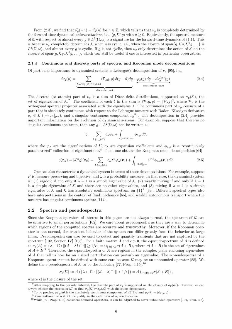
Figure 1: The ε-pseudospectra for the non-linear pendulum and ε = 0.25 (shaded region) computedusing Algorithm 3 with discretization sizes NK . Discretization sizes correspond to a hyperbolic crossapproximation (see Section 4.3.1). The computed ε-pseudospectra converge as NK → ∞. The unitcircle (red line) is shown with the EDMD eigenvalues (magenta dots), many of which are spurious. Ouralgorithm called ResDMD removes spurious eigenvalues by computing pseudospectra (see Section 4).

Pseudospectra allow us to detect so-called spectral pollution, which are spurious eigenvalues that arecaused by discretization and have no relation with the underlying Koopman operator. Spectral pollutioncan cluster at points not in the spectrum of K, even when K is a normal operator, as well as persist as thediscretization size increases [58]. For example, consider the dynamical system of the nonlinear pendulum.Let xxx = (x1, x2) = (θ, θ) be the state variables governed by the following equations of motion:

x1 = x2, x2 = − sin(x1), with Ω = [−π, π]per × R, (2.6)

where ω is the standard Lebesgue measure. We consider the corresponding discrete-time dynamicalsystem by sampling with a time-step ∆t = 0.5. The system is Hamiltonian and hence the Koopmanoperator is unitary. It follows that σε(K) = z ∈ C : dist(z,T) ≤ ε. Fig. 1 shows the pseudospectrumcomputed using Algorithm 3 for ε = 0.25 (see Section 4.3.1). The algorithm uses a discretization sizeof NK to compute a set guaranteed to be inside the ε-pseudospectrum (i.e., no spectral pollution), thatalso converges as NK →∞. We also show the corresponding EDMD eigenvalues. Some of these EDMDeigenvalues are reliable, but the majority are not, demonstrating severe spectral pollution. Note that thisspectral pollution has nothing to do with any stability issues, but instead is due to the discretization ofthe infinite-dimensional operator K by a finite matrix. Using the pseudospectrum for different ε, we candetect exactly which of these eigenvalues are reliable (see Algorithm 2).

3 Computing spectral measures from trajectory data

Throughout this section, we assume that the Koopman operatorK is associated with a measure-preservingdynamical system, and hence is an isometry. We aim to compute smoothed approximations of νg, evenin the presence of continuous spectra, from trajectory data of the dynamical system. More precisely, wewant to select a smoothing parameter ε > 0 and then compute a smooth periodic function νεg such thatfor any bounded, continuous periodic function φ we have [13, Ch. 1]∫

[−π,π]per

φ(θ)νεg(θ) dθ ≈∫

[−π,π]per

φ(θ) dνg(θ). (3.1)

Moreover, as ε → 0, we would like our smoothed function νεg to approach νg in the weak convergencesense implied by (3.1).11 We describe an algorithm that achieves this from trajectory data (see Algo-rithm 1). The algorithm deals with general spectral measures, including those with a singular continuouscomponent. We also evaluate approximations of the density ρg in the pointwise sense and can evaluatethe atomic part of νg, which corresponds to the discrete eigenvalues and eigenfunctions of K.

11Since∫[−π,π]per

φ(θ) dνg(θ) = 〈φ(−i log(K))g, g〉, this convergence also approximates the functional calculus of K. For

example, if the dynamical system (1.1) corresponds to sampling a continuous time dynamical system at discrete time-steps,one could use (3.1) to recover spectral properties of Koopman operators that generate continuous time dynamics.

7

3.1 Computing autocorrelations from trajectory data

We want to collect trajectory data from (1.1) and from this recover as much information as possible aboutthe spectral measure and spectra of K. We assume that (1.1) is observed for M2 time-steps, starting atM1 initial conditions. It is helpful to view the trajectory data as an M1 ×M2 matrix, i.e.,

Bdata =

xxx

(1)0 · · · xxx

(1)M2−1

.... . .

...

xxx(M1)0 · · · xxx

(M1)M2−1

. (3.2)

Each row of Bdata corresponds to an observation of a single trajectory of the dynamical system that iswitnessed for M2 time-steps. In particular, we have xxx

(j)i+1 = F (xxx

(j)i ) for 0 ≤ i ≤M2 − 2 and 1 ≤ j ≤M1.

There are two main ways that trajectory data might be collected: (1) Experimentally-determinedinitial states of the dynamical system, where one must do the best one can with predetermined initialstates, and (2) Algorithmically-determined initial states, where the algorithm can select the initial statesand then record the dynamics. When recovering properties of K, often it is best to have lots of initialstates that explore the whole state-space Ω with a preference of having M1 large and M2 small. If M2 istoo large, then each trajectory could quickly get trapped in attracting states, making it difficult to recoverthe global properties of K. In Sections 3 to 5, we focus on the situation where we have algorithmically-determined initial states and in Section 6 we consider an application with experimental-determined initialstates. The type of trajectory data determines how autocorrelations are calculated.

3.1.1 Algorithmically-determined initial states

For trajectory data collected from algorithmically-determined initial states, there are three main ways to

select the initial conditions, i.e., the values of xxx(j)0 for 1 ≤ j ≤M1, and three complementary approaches

for computing autocorrelations.

1. Initial conditions at quadrature nodes: Suppose that xxx(j)0

M1j=1 are selected so that they are

an M1-point quadrature rule with weights wjM1j=1. Integrals and inner-products can then be ap-

proximated with numerical integration by evaluating functions at the data points. This means thatautocorrelations that determine νg (see Section 2.1.3) can be approximated as

〈g,Kng〉 =

∫Ω

g(xxx)[Kng](xxx) dω(xxx) ≈M1∑j=1

wjg(xxx(j)0 )[Kng](xxx

(j)0 ) =

M1∑j=1

wjg(xxx(j)0 )g(xxx

(j)n ), n ≥ 0.

High-order quadrature rules can lead to fast rates of convergence. If Kng is analytic in a neighborhoodof Ω, then we can often select a quadrature rule that even converges exponentially as M1 →∞ [104].

2. Random initial conditions: Suppose that xxx(j)0

M1j=1 are drawn independently at random from a

fixed probability distribution over Ω that is absolutely continuous with respect to ω with a sufficientlyregular Radon–Nikodym derivative κ. Then, the autocorrelations of K can be approximated usingMonte–Carlo integration, i.e.,

〈g,Kng〉 ≈ 1

M1

M1∑j=1

κ(xxx(j)0 )g(xxx

(j)0 )[Kng](xxx

(j)0 ) =

1

M1

M1∑j=1

κ(xxx(j)0 )g(xxx

(j)0 )g(xxx

(j)n ).

This typically converges at a rate of O(M−1/21 ) [26], but is a practical approach if the state-space

dimension is large. One could also consider quasi-Monte Carlo integration, which can achieve a fasterrate of O(M−1

1 ) (up to logarithmic factors) under suitable conditions [26].

3. A single fixed initial condition: Intuitively, a system is ergodic if any trajectory eventually visitsall parts of state-space. Formally, this means that F in (1.1) is measure-preserving, ω is a probabilitymeasure, and if A is a Borel measurable subset of Ω with xxx : F (xxx) ∈ A ⊂ A, then ω(A) = 0 orω(A) = 1. If a dynamical system is ergodic, then Birkhoff’s ergodic theorem [14] implies that

〈g,Kng〉 = limM2→∞

1

M2 − n

M2−n−1∑j=0

g(xxxj)[Kng](xxxj) = limM2→∞

1

M2 − n

M2−n−1∑j=0

g(xxxj)g(xxxj+n), (3.3)

8

for almost any initial condition xxx0.12 However, the sampling scheme in (3.3) is restricted to ergodicdynamical systems and often requires very long trajectories (see [44] for convergence rates).

If one is entirely free to select the initial conditions of the trajectory data, and d is not too large,then we recommend picking them based on a high-order quadrature rule (see Sections 4.1.3 and 4.3.2).When the state-space dimension d is moderately large we can use sparse grids (see Section 4.3.3) and akernelized approach for large d (see Section 6). One may also want to study the dynamics near attractors.In this case, M1 small and M2 large can be ideal with ergodic sampling [55, Section 7.2].

3.1.2 Experimentally-determined trajectory data

For experimental data, we have no control over the initial conditions, and we may need to combine theabove methods of computing autocorrelations. Often it is assumed that the initial conditions correspondto random initial conditions. We deal with two examples of real-world data sets in Section 6.

3.2 Recovering the spectral measure from autocorrelations

We now suppose that one has already computed the autocorrelations 〈g,Kng〉 for 0 ≤ n ≤ N andwould like to recover a smoothed approximation of νg. Since the Fourier coefficients of νg are given byautocorrelations (see (2.2)), the task is similar to Fourier recovery [1,37]. We are particularly interestedin approaches with good convergence properties as N → ∞, as this reduces the number of computedautocorrelations and the sample size M = M1M2 required for good recovery of the spectral measure.

Motivated by the classical task of recovering a continuous function by its partial Fourier series [32],we start by considering the “windowing trick” from sampling theory. That is, we define a smoothedapproximation to νg as

νg,N (θ) =

N∑n=−N

ϕ( nN

)νg(n)einθ =

1

2π

−1∑n=−N

ϕ( nN

)〈g,K−ng〉einθ +

1

2π

N∑n=0

ϕ( nN

)〈g,Kng〉einθ. (3.4)

The function ϕ : [−1, 1]→ R is often called a filter function [41,100]. The idea of ϕ is that ϕ(x) is closeto 1 when x is close to 0, and ϕ tapers to 0 near x = ±1. By carefully tapering ϕ, the partial sum in (3.4)converges to νg as N →∞ (see Section 3.4). For fast pointwise or weak convergence of νg,N to νg, it isdesirable for ϕ to be an even function that smoothly tapers from 1 to 0.

One of the simplest filters is the hat function ϕhat(x) = 1 − |x|, where (3.4) corresponds to theclassical Cesaro summation of Fourier series. With this choice of ϕ, νg,N (θ) is the convolution of νg withthe famous Fejer kernel, i.e., FN (θ) =

∑Nn=−N (1− |n|/N)einθ. From this viewpoint, the fact that νg,N

weakly converges to νg is immediate from Parseval’s formula [47, Section 1.7]. In particular, for anyLipschitz continuous test function φ with Lipschitz constant L, we have

|φ(θ)− [φ ∗ FN ](θ)| ≤∫

[−π,π]per

|φ(θ − s)− φ(θ)|︸ ︷︷ ︸≤L|s|

FN (s) ds ≤ 2L

N

∫ π

0

s1− cos(Ns)

1− cos(s)ds,

where we used the fact that FN is non-negative and integrates to one. Since we can bound s2/(1−cos(s))from above by π2/2 for s ∈ [0, π], we have the following error bound:∣∣∣∣∣∫

[−π,π]per

φ(θ) dνg(θ)−∫

[−π,π]per

φ(θ)νg,N (θ) dθ

∣∣∣∣∣ ≤ π2L

N

∫ πN

0

1− cos(x)

xdx = O(N−1 log(N)), (3.5)

where we performed a change of variables and used Fubini’s theorem. Therefore, there is slow weakconvergence of νg,N to νg as N → ∞, providing us with an algorithm for ensuring (3.1) with ε = 1/N .Algorithm 1 summarizes our computational framework for recovering a smoothed version of νg fromautocorrelations of the trajectory data.

Other filter functions can provide a faster rate of convergence than ϕhat(x) = 1 − |x|, including thecosine and fourth-order filters [37,106]:

ϕcos(x) =1

2(1− cos(πx)), ϕfour(x) = 1− x4(−20|x|3 + 70x2 − 84|x|+ 35).

12Here we mean ω-almost any initial condition. Though, in practice, it often holds in the Lebesgue sense for almost allinitial conditions and hence one can pick xxx0 at random from a uniform distribution over Ω.

9

Algorithm 1 A computational framework for recovering an approximation of the spectral measure νgassociated with a Koopman operator that is an isometry.

Input: Trajectory data, a filter ϕ, and an observable g ∈ L2(Ω, ω).

1: Approximate the autocorrelations an = 12π 〈g,K

ng〉 for 0 ≤ n ≤ N . (The precise value of N and theapproach depends on the trajectory data (see Section 3.1).)

2: Set a−n = an for 1 ≤ n ≤ N .

Output: The function νg,N (θ) =∑Nn=−N ϕ

(nN

)ane

inθ that can be evaluated for any θ ∈ [−π, π]per.

101

102

103

10-15

10-10

10-5

100

Weak Convergence Error

N

ϕhat

ϕcos

ϕfour

ϕbump

101

102

103

10-15

10-10

10-5

100

Pointwise Error

N

ϕhat

ϕcos

ϕfour

ϕbum

p

Figure 2: Relative errors between νg,N and νg for the shift operator computed with filters ϕhat (blue),ϕcos (red), ϕfour (yellow), and ϕbump (purple). Left: Relative error between νg,N to νg in the senseof (3.5), illustrating weak convergence in (3.1) for the test function φ(θ) = cos(5θ)/(2 + cos(θ)). Right:Relative error between νg,N to ρg at θ = 0, illustrating pointwise convergence. The errors are calculatedusing an exact analytical expression for νg.

For the recovery of measures, we find that a particularly good choice is

ϕbump(x) = exp

(− 2

1− |x|exp

(− c

x4

)), c ≈ 0.109550455106347, (3.6)

where the value of c is selected so that ϕbump(1/2) = 1/2. This filter can lead to arbitrary high orders ofconvergence with errors between νg,N and νg that go to zero faster than any polynomial in N−1(see Sec-tion 3.4). A further useful property is that νg,N localizes any singular behavior of νg (see Section 5.1.3).13

To demonstrate the application of various filters for the recovery of spectral measures from autocorre-lations, we consider the pedagogical dynamical system given by the shift operator. The observed ordersof convergence of Algorithm 1 are predicted by our theory (see Section 3.3).

Example 3.1 (Shift operator). Consider the shift operator with state-space Ω = Z (and counting measureω) given by

xn+1 = F (xn), F (x) = x+ 1.

We seek to compute the spectral measure νg with respect to g ∈ L2(Z, ω) = `2(Z), where `2(Z) is the spaceof square summable doubly infinite vectors. This example is a building block of many dynamical systems,such as Bernoulli shifts, with so-called Lebesgue spectrum [5, Chapter 2]. We consider the observableg(k) = C sin(k)/k, where C ≈ 0.564189583547756 is a normalization constant so that ‖g‖ = 1. Forthis example, νg is absolutely continuous but ρg has discontinuities at θ = ±1. Fig. 2 shows the weakconvergence (left) and pointwise convergence (right) for various filters.

3.3 High-order kernels for spectral measure recovery

To develop convergence theory for Algorithm 1, we view filtering in the broader context of convolutionwith kernels. This provides a unified framework with Section 5 and simplifies the arguments whenanalyzing the recovery of measures (that may be highly singular), as opposed to the recovery of functions.

13This because the kernel associated with ϕbump (see Proposition 3.1) is highly localized due to the smoothness of ϕbump.

10

Instead of viewing νg,N as constructed by “windowing” the Fourier series of νg in (3.4) by a filter, weform an approximation to νg by convolution. That is, we define

νεg(θ0) =

∫[−π,π]per

Kε(θ0 − θ)dνg(θ),

where Kε are a family of integrable functions Kε : 0 < ε ≤ 1 satisfying certain properties (see Def-inition 3.1) so that νεg converges to νg in some sense. It is easy to verify that νεg = νg,N whenKε(θ) = 1

2π

∑Nn=−N ϕ

(nN

)einθ and N = bε−1c, say. The most famous example of Kε is the Poisson

kernel for the unit disc given by [47, p.16]

Kε(θ) =1

2π

(1 + ε)2 − 1

1 + (1 + ε)2 − 2(1 + ε) cos(θ), (3.7)

in polar coordinates with r = (1 + ε)−1. The Poisson kernel is a first-order kernel because, up to alogarithmic factor, it leads to a first-order algebraic rate of convergence of νεg to νg. We now give thefollowing general definition of an mth order kernel, and justify their name by showing that they lead toan mth order rate of convergence of νεg to νg in a weak and pointwise sense (see Section 3.4).

Definition 3.1 (mth order periodic kernel). Let Kε : 0 < ε ≤ 1 be a family of integrable functions onthe periodic interval [−π, π]per. We say that Kε is an mth order kernel for [−π, π]per if

(i) (Normalized)∫

[−π,π]perKε(θ) dθ = 1.

(ii) (Approximately vanishing moments) There exists a constant CK such that14∣∣∣∣∣∫

[−π,π]per

θnKε(θ) dθ

∣∣∣∣∣ ≤ CKεm log(ε−1), for any integer 1 ≤ n ≤ m− 1. (3.8)

(iii) (Decay away from 0) For any θ ∈ [−π, π] and 0 < ε ≤ 1,

|Kε(θ)| ≤CKε

m

(ε+ |θ|)m+1. (3.9)

The conditions in Definition 3.1 are mostly technical assumptions that allow one to prove appropriateconvergence rates of νεg to νg. For pointwise convergence, property (iii) is required to apply a local cut-offargument away from singular parts of the measure. Properties (i) and (ii) are used to show that termsvanish in a local Taylor series expansion of the Radon–Nikodym derivative, and the remainder is boundedby (iii). For weak convergence, we apply similar arguments to the test function by Fubini’s theorem.

The properties of an mth order kernel can be translated to properties of a filter.

Proposition 3.1. Let m ∈ N and suppose that ϕ is an even continuous function that is compactlysupported on [−1, 1] such that (a) ϕ ∈ Cm−1([−1, 1]), (b) ϕ(0) = 1 and ϕ(n)(0) = 0 for any integer1 ≤ n ≤ m− 1, (c) ϕ(n)(1) = 0 for any integer 0 ≤ n ≤ m− 1, and (d) ϕ|[0,1] ∈ Cm+1([0, 1]). Then,

Kε(θ) =1

2π

N∑n=−N

ϕ( nN

)einθ, N = bε−1c (3.10)

is an mth order kernel for [−π, π]per.

Proof. We need to verify that Kε in (3.10) satisfies the three properties in Definition 3.1. It is easy tosee that Kε is normalized by integrating (3.10) term-by-term and noting that ϕ(0) = 1.

For property (iii), we define Φ(k) =∫ 1

−1ϕ(x)eikx dx and note that by the Poisson summation formula

we have Kε(θ) = N2π

∑∞j=−∞ Φ(N(θ + 2πj)). Using the fact that ϕ is an even function, we have Φ(k) =

2∫ 1

0ϕ(x) cos(kx) dx and since ϕ satisfies (b), (c) and (d), we find that for k 6= 0

|Φ(k)| = 2

km

∣∣∣∣∫ 1

0

ϕm(x) cos(kx) dx

∣∣∣∣ , if m is even,∣∣∣∣∫ 1

0

ϕm(x) sin(kx) dx

∣∣∣∣ , if m is odd.

14One may wonder if insisting on exactly vanishing moments or removing the logarithmic term improves convergencerates as ε ↓ 0. This is not the case - see the discussion in Section 3.4.

11

Finally, one can use property (d) to perform integration-by-parts (now with possibly non-vanishingendpoint conditions) to deduce that |Φ(k)| . (1 + |k|)−(m+1). Therefore, we find that

|Kε(θ)| .∞∑

j=−∞

N

(1 + |N(θ + 2πj)|)m+1.

N

(1 +N |θ|)m+1.

This bound implies the decay condition in (3.9).For property (ii), note that for any N ≥ |n|, we have the following analytical expression:∫

[−π,π]per

Kε(−θ)einθ dθ − 1 = ϕ( nN

)− ϕ(0), N = bε−1c.

By using Taylor’s theorem and ϕ(j)(0) = 0, we have∣∣∣∣∣∫

[−π,π]per

Kε(−θ)einθ dθ − 1

∣∣∣∣∣ ≤ nm‖ϕ|(m)[0,1]‖L∞

m!Nm= O (εm) as ε→ 0.

The result now follows from Lemma A.1.

Therefore, it can be verified that: ϕhat, ϕcos, and ϕfour induce first-order, second-order and fourth-order kernels in (3.10), respectively. Similarly, ϕbump induces a kernel that is mth order for any m ∈ N.For example, up to a logarithmic factor, the rate of convergence between νεg (resp. νg,N ) and νg for ϕfour

is O(ε4) as ε→ 0 (resp. O(N−4) as N →∞) in a weak and pointwise sense (see Section 3.4).Readers who are experts on filters may be surprised by condition (d) in Proposition 3.1. This ad-

ditional condition, which holds for all common choices of filters, is theoretically needed to obtain theoptimal convergence rates between νεg and νg. It means that our convergence theory is one algebraicorder better than the convergence theorems derived in the literature [37, Theorem 3.3].

3.4 Convergence results

We now provide convergence theorems for the recovery of the spectral measure of K. A reader concernedwith only the practical aspects of our algorithms can safely skip over this section while appreciating thatthe convergence guarantees are rigorous.

3.4.1 Pointwise convergence

For a point θ0 ∈ [−π, π], the value of the approximate spectral measure νεg(θ0) converges to the Radon–Nikodym derivative, ρg(θ0) provided that νg is absolutely continuous in an interval containing θ0 (withoutthis separation condition it still converges for almost every θ0). The precise rate of convergence dependson the smoothness of ρg in a small interval I containing θ0. In particular, we write ρg ∈ Cn,α(I) if ρgis n-times continuously differentiable on I and the nth derivative is Holder continuous with parameter0 ≤ α < 1. For h1 ∈ C0,α(I) and h2 ∈ Ck,α(I) we define the seminorm and norm, respectively, as

|h1|C0,α(I) = supx 6=y∈I

|h1(x)− h1(y)||x− y|α

, ‖h2‖Ck,α(I) = |h(k)2 |C0,α(I) + max

0≤j≤k‖h(j)

2 ‖∞,I .

We state the following pointwise convergence theorem for general complex-valued measures ν as we applyit to measures corresponding to test functions to prove Theorem 3.2. The choice ν = νg with ‖νg‖ = 1in Theorem 3.1 gives pointwise convergence of spectral measures.

Theorem 3.1 (Pointwise convergence). Let Kε be an mth order kernel for [−π, π]per and let ν be acomplex-valued measure on [−π, π]per with finite total variation ‖ν‖. Suppose that for some θ0 ∈ [−π, π]and η ∈ (0, π), ν is absolutely continuous on I = (θ0 − η, θ0 + η) with Radon–Nikodym derivativeρ ∈ Cn,α(I) (α ∈ [0, 1)). Then the following hold for any 0 ≤ ε < 1:

(i) If n+ α < m, then∣∣∣∣∣ρ(θ0)−∫

[−π,π]per

Kε(θ0 − θ) dν(θ)

∣∣∣∣∣ . CK(‖ν‖+ ‖ρ‖Cn,α(I)

)(εn+α +

εm

(ε+ η)m+1

)(1 + η−n−α

).

(3.11)

12

(ii) If n+ α ≥ m, then∣∣∣∣∣ρ(θ0)−∫

[−π,π]per

Kε(θ0 − θ) dν(θ)

∣∣∣∣∣ . CK(‖ν‖+ ‖ρ‖Cm(I)

)(εm log(ε−1) +

εm

(ε+ η)m+1

)(1 + η−m

).

(3.12)

Here, ‘.’ means that the inequality holds up to a constant that only depends on n+ α and m.

Proof. By periodicity, we can assume without loss of generality that θ0 = 0. First, we decompose ρ intotwo parts ρ = ρ1 +ρ2, where ρ1 ∈ Cn,α(I) is compactly supported on I and ρ2 vanishes on (−η/2,+η/2).Using (3.9), we have∣∣∣∣∣ρ(0)−

∫[−π,π]per

Kε(−θ)dν(θ)

∣∣∣∣∣ ≤∣∣∣∣∣ρ1(0)−

∫[−π,π]per

Kε(−θ)ρ1(θ) dθ

∣∣∣∣∣+

∫|θ|>η/2

CKεm d|νr|(θ)

(ε+ η/2)m+1, (3.13)

where dνr(θ) = dν(θ) − ρ1(θ) dθ. The second term on the right-hand side of (3.13) is bounded byC1CK(‖ν‖+ ‖ρ1‖L∞(I))ε

m(ε+ η)−(m+1) for some constant C1 independent of all parameters. To boundthe first term, we expand ρ1 using Taylor’s theorem:

ρ1(θ) =

k−1∑j=0

ρ(j)1 (0)

j!θj +

ρ(k)1 (ξθ)

k!θk, k = min(n,m), (3.14)

where |ξθ| ≤ |θ|. We now consider the two cases of the theorem separately.Case (i): n + α < m. In this case, k = n and we can select ρ1 so that,

‖ρ1‖Cn,α(I) ≤ C(n, α)‖ρ‖Cn,α(I)

(1 + η−n−α

), ‖ρ1‖L∞(I) ≤ C(n, α)‖ρ‖Cn,α(I) (3.15)

for some universal constant C(n, α) that only depends on n and α. Existence of such a decompositionfollows from standard arguments with cut-off functions. Using (3.14), part (ii) of Definition 3.1 and thefirst bound of (3.15), we obtain∣∣∣∣∣ρ1(0)−

∫[−π,π]per

Kε(−θ)ρ1(θ) dθ

∣∣∣∣∣ ≤C2CK‖ρ‖Cn,α(I)εm log(ε−1)

(1 + η−n−α

)+

∣∣∣∣∣∫

[−π,π]per

Kε(−θ)ρ

(n)1 (ξθ)− ρ(n)

1 (0)

n!θn dθ

∣∣∣∣∣ ,(3.16)

for some constant C2 independent of ε, η and ν (or ρ, ρ1, ρ2). Note that we have added the factor of

ρ(n)1 (0) into the integrand by a second application of part (ii) of Definition 3.1 and the fact that n < m.

The Holder continuity of ρ(n)1 implies that |ρ(n)

1 (ξθ)− ρ(n)1 (0)| ≤ C(n, α)‖ρ‖Cn,α(I) (1 + η−n−α) θα. Using

this bound in the integrand on the right-hand side of (3.16) and (3.9), we obtain∣∣∣∣∣ρ1(0)−∫

[−π,π]per

Kε(−θ)ρ1(θ) dθ

∣∣∣∣∣ ≤ C3CK‖ρ‖Cn,α(I)

(εm log(ε−1) + εn+α

∫ π/ε

0

τn+αdτ

(1 + τ)m+1

)(1+η−n−α

),

for some constant C3 independent of ε, η and ν (or ρ, ρ1, ρ2). Since m > n+ α, the integral in bracketsconverges as ε ↓ 0 and the bound in (3.11) now follows.

Case (ii): n + α ≥m. In this case, k = m and we can select ρ1 such that

‖ρ1‖Cm(I) ≤ C(m)‖ρ‖Cm(I)

(1 + η−m

),

for some universal constant C(m) that only depends on m. Again, existence of such a decompositionfollows from standard arguments with cut-off functions. Using (3.14) and applying (3.8) to the powersθj for j < m and (3.9) to the θm term, we obtain∣∣∣∣∣ρ1(0)−

∫[−π,π]per

Kε(−θ)ρ1(θ) dθ

∣∣∣∣∣ ≤ C2CK‖ρ‖Cm(I)

(εm log(ε−1) + εm

∫ π/ε

0

τmdτ

(1 + τ)m+1

)(1 + η−m

),

for some constant C2 independent of ε, η and ν (or ρ, ρ1, ρ2). The bound in (3.12) now follows.

The logarithmic term in (3.12) is due to the integral∫ π/ε

0τmdτ

(1+τ)m+1 and cannot, in general, be removed

even with exactly vanishing moments replacing (3.8).

13

3.4.2 Weak convergence

We now turn to proving weak convergence in the sense of (3.1). Using Theorem 3.1 and a dualityargument, we can also provide rates of convergence for (3.1).

Theorem 3.2 (Weak convergence). Let Kε be an mth order kernel for [−π, π]per, φ ∈ Cn,α([−π, π]per),and let νg be a spectral measure on the periodic interval [−π, π]per. Then∣∣∣∣∣

∫[−π,π]per

φ(θ)νεg(θ) dθ −∫

[−π,π]per

φ(θ) dνg(θ)

∣∣∣∣∣ . CK‖φ‖Cn,α([−π,π]per)

(εn+α + εm log(ε−1)

), (3.17)

where ‘.’ means that the inequality holds up to a constant that only depends on n+ α and m.

Proof. Let Kε(θ) = Kε(−θ), then it is easily seen that Kε is an mth order kernel for [−π, π]per. Fubini’stheorem allows us to exchange order of integration to see that∫

[−π,π]per

φ(θ)νεg(θ) dθ =

∫[−π,π]per

φ(θ)[Kε ∗ νg](θ) dθ =

∫[−π,π]per

[Kε ∗ φ](θ) dνg(θ).

We can now apply Theorem 3.1 to the absolutely continuous measure with Radon–Nikodym derivativeφ and the kernel Kε (e.g., with η = π/2) to see that∣∣∣[Kε ∗ φ](θ)− φ(θ)

∣∣∣ ≤ C1CK‖φ‖Cn,α([−π,π]per)

(εn+α + εm log(ε−1)

),

for some constant C1 depending on n, α and m. Since νg is a probability measure, (3.17) follows.

It is worth noting that the high-order convergence in Theorem 3.2 does not require any regularity as-sumptions on νg. Moreover, though not covered by the theorem, for any mth order kernel and continuousperiodic function φ, weak convergence still holds.

3.4.3 Recovery of the atomic parts of the spectral measure

Finally, we consider the recovery of atomic parts of spectral measures or, equivalently, σp(K) - the setof eigenvalues of K (see (2.4)). This convergence is achieved by rescaling the smoothed approximationKε ∗ νg. The following theorem means that Algorithm 1 convergences to both the eigenvalues of K andthe continuous part of the spectrum of K.

Theorem 3.3 (Recovery of atoms). Let Kε be an mth order kernel for [−π, π]per that satisfies

lim supε↓0ε−1

|Kε(0)| <∞, and let νg be a spectral measure on [−π, π]per. Then, for any θ0 ∈ [−π, π]per, we

have

νg(θ0) = limε↓0

1

Kε(0)[Kε ∗ νg](θ0). (3.18)

Proof. By periodicity, we may assume without loss of generality that θ0 = 0. Let ν′g = νg − νg(0)δ0,then

1

Kε(0)[Kε ∗ νg](0) = νg(0) +

1

Kε(0)[Kε ∗ ν′g](0). (3.19)

Consider the function Kε(−θ)/Kε(0), which is uniformly bounded for sufficiently small ε using (3.9) and

the assumption lim supε↓0ε−1

|Kε(0)| <∞. Since limε↓0Kε(−θ)/Kε(0) = 0 for any θ 6= 0 and ν′g(0) = 0,

limε↓0

1

Kε(0)[Kε ∗ ν′g](0) = lim

ε↓0

∫[−π,π]per

Kε(−θ)Kε(0)

dν′g = 0,

where we used the dominated convergence theorem. Using (3.19), the theorem now follows.

The condition that lim supε↓0ε−1

|Kε(0)| < ∞ is a technical condition that is satisfied by all the kernels

constructed in this paper. A condition like this is required to recover the atomic part of νg as it saysthat Kε must become localized around 0 sufficiently quickly as ε→ 0.

3.5 Numerical examples

We now consider two numerical examples of Algorithm 1 and the convergence theory in Section 3.4.

14

-3 -2 -1 0 1 2 310

-2

10-1

100

101

ν100g (θ)

θ

?

ρg

Eigenvalue

-3 -2 -1 0 1 2 310

-2

10-1

100

101

-1 -0.95 -0.9 -0.85 -0.810

-5

100

ν1000g (θ)

θ

Figure 3: Computed approximate spectral measures with respect to the function g in (3.20) using Algo-rithm 1 with the filter in (3.6) for the tent map. These are computed with (blue) and without (red) thefilter in (3.6) for discretization sizes N = 100 (left) and N = 1000 (right). The function νg,N is highlyoscillatory if no filter is used (see zoomed in subplot).

3.5.1 Tent map

The tent map with parameter 2 is the function F : [0, 1] → [0, 1] given by F (x) = 2 minx, 1 − x. Itgenerates a chaotic system with discrete and continuous spectra. We consider Ω = [0, 1] with the usualLebesgue measure. The corresponding Koopman operator K is an isometry, but it is not unitary sincethe function Kg is symmetric about x = 1/2 for any function g, and hence K is not onto. Furthermore,

the decomposition in (2.4) reduces to an atomic part at θ = 0 of size (∫ 1

0g(x)dx)2 and an absolutely

continuous part. The tent map thus demonstrates that our algorithm deals with mixed spectral typeswithout a priori knowledge of the eigenvalues of K.

To compute the inner-products 〈g,Kng〉 for Algorithm 1, we sample the observable g on an equallyspaced dyadic grid with equal weights.15 As an example, consider the arbitrary discontinuous function

g(θ) = C|θ − 1/3|+ C sin(20θ) +

C, θ > 0.78,

0, θ ≤ 0.78,(3.20)

where C ≈ 1.035030525813683 is a normalization constant. Applying Algorithm 1, we found convergenceto the Radon–Nikodym derivative away from the singular part of the measure (the atom at zero) behavedas predicted by Theorem 3.1. To see the importance of the filter, we have plotted the reconstructionfrom the Fourier coefficients both with and without the filter (3.6) in Fig. 3. As N increases, we seethat the filter localizes the severe oscillations in the vicinity of the origin and we gain convergence to theRadon–Nikodym derivative away from the eigenvalue at 0. This is not the case without the filter, wheresevere oscillations pollute the entire interval. Using the filter in (3.6), the atomic part approximatedvia Theorem 3.3 was correct to 4.4 × 10−4 for N = 1000 and converges in the limit N → ∞, whereasconvergence via (3.18) does not hold without the filter.

Finally, we consider the sample complexity M1M2 needed to recover the Fourier coefficients of themeasures. We consider the maximum absolute error of the computed νg(n) for |n| ≤ 10 for our quadraturebased method and the ergodic sampling method from (3.3). For the ergodic method, M1 = 1 andhence the sample complexity is the length of the trajectory used. However, for this example, the naiveapplication of (3.3) for the ergodic method is severely unstable. Due to the binary nature of the tentmap, each application of F loses a single bit of precision. Using floating-point arithmetic means thattrajectories eventually stagnate at the fixed point 0. This error is not a random numerical error but astructured one. A good solution is to perturb each evaluation of F by a small random amount. Theinstability is not present for tent map parameters that avoid exact binary representations. Fig. 4 shows

the results for a range of different g. The ergodic method converges like O(M−1/22 ) as M2 →∞ and the

quadrature based method converges with a faster rate in M1.

15While this quadrature rule may seem suboptimal, it is selected due to the dyadic structure of the tent map and toavoid issues when computing the integrals 〈g,Kng〉 for large n due to chaotic nature of F .

15

101

102

103

104

10-5

10-4

10-3

10-2

10-1

100

Error, g from (3.20)

O((M1M

2) −1)

O((M1M

2)−1/2)

M1M2

101

102

103

104

10-8

10-6

10-4

10-2

100

Error, g =√

2 cos(πx− 0.1)

O((M1M

2 ) −2)

O((M1M2)−1/2)

M1M2

101

102

103

104

10-15

10-10

10-5

100

Error, g =√

2 cos(100πx)

O((M1M2)−1/2)

M1M2

Figure 4: Maximum absolute error in computing νg(n) for −10 ≤ n ≤ 10 with a sample size of M1M2

for quadrature (blue) and stabilized ergodic (red). Each g is normalized so that ‖g‖ = 1.

-3 -2 -1 0 1 2 3

10-4

10-2

100

102

ν100g (θ)

θ

-3 -2 -1 0 1 2 3

10-4

10-2

100

102

ν1000g (θ)

θ

Figure 5: Computed spectral measure using Algorithm 1 with (3.6) for the nonlinear pendulum.

3.5.2 Nonlinear pendulum

The nonlinear pendulum is a non-chaotic Hamiltonian system with continuous spectra and challengingKoopman operator theory. Here, we consider a corresponding discrete-time system by sampling (2.6) witha time-step of ∆t = 1. We collect M1 data points on an equispaced tensor product grid correspondingto the periodic trapezoidal quadrature rule in the x1 direction and a truncated16 trapezoidal quadraturerule in the x2 direction. To simulate the collection of trajectory data, we compute trajectories startingat each initial condition using the ode45 command in MATLAB.

We look at the following observable that involves non-trivial dynamics in each coordinate:

g(x1, x2) = C(1 + i sin(x1))(1−√

2x2)e−x22/2,

where C ≈ 0.24466788518668 is a normalization constant. Fig. 5 shows high resolution approximationsof the spectral measure corresponding νg for N = 100 using M1 = 50000 and N = 1000 using M1 = 106.The spectral measure has a continuous component away from θ = 0. Note that the constant function 1 isnot in L2([0, 2π]per×R) and hence cannot be an eigenfunction. We confirmed this by using Theorem 3.3for larger N and observing that the peak in Fig. 5 (left) does not grow as fast as ∝ N . However, thereis a singular component of the spectral measure at θ = 0.

There are two challenges associated with Algorithm 1 when N is large. First, M1 needs to be largeenough to adequately approximate 〈g,Kng〉 for −N ≤ n ≤ N , which is observed in Fig. 5 when we movefrom the left to the right panel. Second, the ode45 command in MATLAB to compute trajectory datais severely limited in the case of chaotic systems, even with tiny time-steps. For chaotic systems (e.g.,double pendulum), the first few Fourier coefficients of νg can be estimated, but long trajectories canquickly become inaccurate. This problem is inherently associated with chaotic systems and occurs forother methods of collecting trajectory data (including experimental). We overcome this by deriving analgorithm to approximate spectral measures νg without needing long trajectories (see Section 5).

16We select a truncation to x2 ∈ [−L,L] so that the g and Kng are negligible for |x2| > L.

16

4 Residual DMD (ResDMD)

In this section, we consider dynamical systems of the form (1.1) that are not necessarily measure-preserving. Therefore, we cannot assume that K is an isometry. We assume that we have access toa sequence of snapshots, i.e., a trajectory data matrix (see (3.2)) with two columns:

Bdata =

xxx

(1)0 xxx

(1)1

......

xxx(M1)0 xxx

(M1)1

, (4.1)

where xxx(j)1 = F (xxx

(j)0 ) for 1 ≤ j ≤M1. An M1 ×M2 trajectory data matrix can be converted to the form

of (4.1) by forgetting that the data came from long runs and reshaping the matrix.Using (4.1) we develop a new algorithm, which we call Residual DMD (ResDMD), that approximates

the associated Koopman operator of the dynamics. Our approach allows for Koopman operators K thathave no finite-dimensional invariant subspace. The key difference between ResDMD and other DMDalgorithms (such as EDMD) is that we construct Galerkin approximations for not only K, but also K∗K.This difference allows us to have rigorous convergence guarantees for ResDMD when recovering spectralinformation of K and computing pseudospectra. In particular, we avoid spectral pollution (see Fig. 1).

4.1 Extended DMD (EDMD) and a new matrix for computing residuals

Before discussing our ResDMD approach, we describe EDMD. EDMD constructs a matrix KEDMD ∈CNK×NK that approximates the action of K from the snapshot data in (4.1). The original description ofEDMD assumes that the initial conditions xxx(j)

0 M1j=1 ⊂ Ω are drawn independently according to ω [110].

Here, we describe EDMD for arbitrary initial states and use xxx(j)0

M1j=1 as quadrature nodes.

4.1.1 EDMD viewed as a Galerkin method

Given a dictionary ψ1, . . . , ψNK ⊂ D(K) of observables, EDMD selects a matrix KEDMD that approxi-

mates K on the subspace VNK = spanψ1, . . . , ψNK, i.e., [Kψj ](xxx) = ψj(F (xxx)) ≈∑NKi=1(KEDMD)ijψi(xxx)

for 1 ≤ j ≤ NK . Define the vector-valued feature map Ψ(xxx) =[ψ1(xxx) · · · ψNK (xxx)

]∈ C1×NK . Then

any g ∈ VNK can be written as g(xxx) =∑NKj=1 ψj(xxx)gj = Ψ(xxx)ggg for some vector ggg ∈ CNK . It follows that

[Kg](xxx) = Ψ(F (xxx))ggg = Ψ(xxx)(KEDMD ggg) +

NK∑j=1

ψj(F (xxx))gj −Ψ(xxx)(KEDMD ggg)

︸ ︷︷ ︸

r(ggg,xxx)

.

Typically, VNK is not an invariant subspace of K so there is no choice of KEDMD that makes r(ggg,xxx)zero for all g ∈ VN and xxx ∈ Ω. Instead, it is natural to select KEDMD as a solution of the followingoptimization problem:

argminB∈CNK×NK

∫Ω

maxggg∈CNK ,‖ggg‖=1

|r(ggg,xxx)|2 dω(xxx) =

∫Ω

‖Ψ(F (xxx))−Ψ(xxx)B‖2`2 dω(xxx)

. (4.2)

Here, ‖ · ‖`2 denotes the standard Euclidean norm of a vector.In practice, one cannot directly evaluate the integral in (4.2) and instead we approximate it via a

quadrature rule with nodes xxx(j)0

M1j=1 and weights wjM1

j=1. The discretized version of (4.2) is thereforethe following weighted least-squares problem:

argminB∈CNK×NK

M1∑j=1

wj

∥∥∥Ψ(xxx(j)1 )−Ψ(xxx

(j)0 )B

∥∥∥2

`2. (4.3)

A solution to (4.3) can be written down explicitly as KEDMD = (Ψ∗0WΨ0)†(Ψ∗0WΨ1), where ‘†’ denotesthe pseudoinverse and W = diag(w1, . . . , wM ). Here, Ψ0 and Ψ1 are the M1 ×NK matrices given by

Ψ0 =[Ψ(xxx

(1)0 )> · · · Ψ(xxx

(M1)0 )>

]>, Ψ1 =

[Ψ(xxx

(1)1 )> · · · Ψ(xxx

(M1)1 )>

]>. (4.4)

17

By reducing the size of the dictionary if necessary, we may assume without loss of generality that Ψ∗0WΨ0

is invertible. In practice, one may also consider regularization through truncated singular value decom-

positions. Since Ψ∗0WΨ0 =∑M1

j=1 wjΨ(xxx(j)0 )∗Ψ(xxx

(j)0 ) and Ψ∗0WΨ1 =

∑M1

j=1 wjΨ(xxx(j)0 )∗Ψ(xxx

(j)1 ), if the

quadrature converges (see Section 4.1.3) then

limM1→∞

[Ψ∗0WΨ0]jk = 〈ψk, ψj〉 and limM1→∞

[Ψ∗0WΨ1]jk = 〈Kψk, ψj〉,

where 〈·, ·〉 is the inner-product associated with L2(Ω, ω). Thus, EDMD can be viewed as a Galerkinmethod in the large data limit as M1 →∞. Let PVNK denote the orthogonal projection onto VNK . In thelarge data limit, KEDMD approaches a matrix representation of PVNKKP

∗VNK

and the EDMD eigenvalues

approach the spectrum of PVNKKP∗VNK

. Thus, approximating σ(K) by the eigenvalues of KEDMD is

closely related to the so-called finite section method [15]. Since the finite section method can suffer fromspectral pollution (see Section 2.2), spectral pollution is also a concern for EDMD17 and it is importantto have an independent way to measure the accuracy of candidate eigenvalue-eigenvector pairs.

4.1.2 Measuring the accuracy of candidate eigenvalue-eigenvector pairs

Suppose that we have a candidate eigenvalue-eigenvector pair (λ, g) ofK, where λ ∈ C and g = Ψggg ∈ VNK .One way to measure the accuracy of (λ, g) is by estimating the squared relative residual, i.e.,∫

Ω|[Kg](xxx)− λg(xxx)|2 dω(xxx)∫

Ω|g(xxx)|2 dω(xxx)

=〈(K − λ)g, (K − λ)g〉

〈g, g〉(4.5)

=

∑NKj,k=1 gjgk

[〈Kψk,Kψj〉 − λ〈ψk,Kψj〉 − λ〈Kψk, ψj〉+ |λ|2〈ψk, ψj〉

]∑NKj,k=1 gjgk〈ψk, ψj〉

.

If K is a normal operator, then the minimum of (4.5) over all normalized g ∈ D(K) is exactly the squaredistance of λ to the spectrum of K; otherwise, for non-normal the residual can still provide a measureof accuracy (see Appendix B). One can also use the residual to bound the distance between g and theeigenspace associated with λ, assuming λ is a point in the discrete spectrum of K [96, Chapter V].

We approximate the residual in (4.5) by

res(λ, g)2 =

∑NKj,k=1 gjgk

[(Ψ∗1WΨ1)jk − λ(Ψ∗1WΨ0)jk − λ(Ψ∗0WΨ1)jk + |λ|2(Ψ∗0WΨ0)jk

]∑NKj,k=1 gjgk(Ψ∗0WΨ0)jk

. (4.6)

All the terms in this residual can be computed using the snapshot data. Note that, as well as the matricesfound in EDMD, (4.6) has the additional matrix Ψ∗1WΨ1. Moreover, under certain conditions, we have

limM1→∞ res(λ, g)2 =∫

Ω|[Kg](xxx)− λg(xxx)|2 dω(xxx)/

∫Ω|g(xxx)|2 dω(xxx) for any g ∈ VNK (see Section 4.1.3).

In particular, we often have limM1→∞[Ψ∗1WΨ1]jk = 〈Kψk,Kψj〉 and then Ψ∗1WΨ1 formally correspondsto a Galerkin approximation of K∗K as M1 → ∞. In Appendix B we show that the quantity res(λ, g)can be used to rigorously compute spectra and pseudospectra of K.

4.1.3 Convergence of matrices in the large data limit

Echoing Section 3.1.1, we focus on three situations when algorithmically-determined snapshot data en-sures that

limM1→∞

[Ψ∗0WΨ0]jk = 〈ψk, ψj〉, limM1→∞

[Ψ∗0WΨ1]jk = 〈Kψk, ψj〉, limM1→∞

[Ψ∗1WΨ1]jk = 〈Kψk,Kψj〉.(4.7)

For initial conditions at quadrature nodes, if the dictionary functions and F are sufficiently regular, then

it is beneficial to select xxx(j)0

M1j=1 as an M1-point quadrature rule with weights wjM1

j=1. This can lead tomuch faster rates of convergence rates in (4.7) (see Section 4.3.2). For example, if Ω is unbounded thenwe can use quadrature rules such as the trapezoidal rule (see Section 4.3.1) and if Ω is a bounded simpledomain then one can use Gaussian quadrature (see Section 4.3.2). When the state-space dimension d

17It was pointed out in [54] that if K is bounded and the corresponding eigenvectors of a sequence of eigenvalues do notweakly converge to zero as the discretization size increases, then the EDMD eigenvalues have a convergent subsequence toan element of the spectrum. Unfortunately, verifying that the eigenvectors do not converge to zero is impossible in practice.

18

Algorithm 2 : ResDMD for computing eigenpairs without spectral pollution.

Input: Snapshot data xxx(j)0

M1j=1, xxx

(j)1

M1j=1 (such that xxx

(j)1 = F (xxx

(j)0 )), quadrature weights wjM1

j=1, a

dictionary of observables ψjNKj=1 and an accuracy goal ε > 0.

1: Compute Ψ∗0WΨ0, Ψ∗0WΨ1, and Ψ∗1WΨ1, where Ψ0 and Ψ1 are given in (4.4).2: Solve (Ψ∗0WΨ1)ggg = λ(Ψ∗0WΨ0)ggg for eigenpairs (λj , g(j) = Ψgggj).3: Compute res(λj , g(j)) for all j (see (4.6)) and discard if res(λj , g(j)) > ε.

Output: A collection of accurate eigenpairs (λj , gggj) : res(λj , g(j)) ≤ ε.

is moderately large we can use sparse grids (see Section 4.3.3) and a kernelized approach for large d(see Section 6).

If ω is a probability measure and the initial points xxx(j)0

M1j=1 are drawn independently and at ran-

dom according to ω, the strong law of large numbers shows that limM1→∞[Ψ∗0WΨ0]jk = 〈ψk, ψj〉 andlimM1→∞[Ψ∗0WΨ1]jk = 〈Kψk, ψj〉 holds with probability one [94, Section 3.4] provided that ω is notsupported on a zero level set that is a linear combination of the dictionary [54, Section 4]. This is with

the quadrature weights wj = 1/M1 and the convergence is typically at a Monte–Carlo rate of O(M−1/21 ).

This argument is straightforward to adapt to show the convergence limM1→∞[Ψ∗1WΨ1]jk = 〈Kψk,Kψj〉.For a single fixed initial condition, if the dynamical system is ergodic, then one can use Birkhoff’s Er-

godic Theorem to show that limM1→∞[Ψ∗0WΨ0]jk = 〈ψk, ψj〉 and limM1→∞[Ψ∗0WΨ1]jk = 〈Kψk, ψj〉 [54].One chooses wj = 1/M1 but the convergence rate is problem dependent [44]. This argument is straight-forward to adapt to show the convergence limM1→∞[Ψ∗1WΨ1]jk = 〈Kψk,Kψj〉.

4.2 ResDMD: Avoiding spectral pollution and computing pseudospectra

We now present our first ResDMD algorithm that computes the residual using the snapshot data toavoid spectral pollution. As is usually done, the algorithm assumes that KEDMD is diagonalizable. First,we compute the three matrices Ψ∗0WΨ0, Ψ∗0WΨ1, and Ψ∗1WΨ1, where Ψ0 and Ψ1 are given in (4.4).Then, we find the eigenvalues and eigenvectors of KEDMD, i.e., we solve (Ψ∗0WΨ0)†(Ψ∗0WΨ1)ggg = λggg.One can solve this eigenproblem directly, but it is often numerical more stable to solve the generalizedeigenvalue problem (Ψ∗0WΨ1)ggg = λ(Ψ∗0WΨ0)ggg. Afterwards, to avoid spectral pollution, we discardcomputed eigenpairs with a larger relative residual than an accuracy goal of ε > 0.

Algorithm 2 summarizes the procedure and is a simple modification of EDMD as the only difference isa clean-up where spurious eigenpairs are discarded based on their residual. This clean-up avoids spectralpollution and removes eigenpairs that are inaccurate due to numerical errors associated with non-normaloperators, up to the relative tolerance of ε. The following result makes this precise.

Theorem 4.1. Let K be the associated Koopman operator of (1.1) from which snapshot data is collected.Let ΛM1 denote the eigenvalues in the output of Algorithm 2. Then, assuming (4.7), we have

lim supM1→∞

maxλ∈ΛM1

‖(K − λ)−1‖−1 ≤ ε.

Proof. Seeking a contradiction, assume that lim supM1→∞maxλ∈ΛM1‖(K − λ)−1‖−1 > ε. Then, there

is a subsequence of eigenpairs (λk, gggk) in the output of Algorithm 2 (with M1 = nk) such that λk ∈Λnk , nk → ∞, and ‖(K − λk)−1‖−1 > ε + δ for some δ > 0 and all k. Since (4.7) is satisfied andKEDMD = (Ψ∗0WΨ0)†(Ψ∗0WΨ1) is a sequence of bounded finite matrices (recall that without loss ofgenerality the Gram matrix limM1→∞Ψ∗0WΨ0 is invertible), the sequence λ1, λ2, . . . , stays bounded. Bytaking a subsequence if necessary, we may assume that limk→∞ λk = λ. We must have that

ε+ δ ≤ ‖(K − λ)−1‖−1 = limk→∞

‖(K − λk)−1‖−1 ≤ lim supk→∞

res(λk, gggk) ≤ ε,

which is the desired contradiction.

In the large data limit, Theorem 4.1 tells us that ResDMD computes eigenvalues inside the ε-pseudospectrum of K and hence, avoids spectral pollution and returns reasonable eigenvalues. Despitethis, Algorithm 2 may not approximate the whole ε-pseudospectrum of K even as M1 →∞ and NK →∞because the eigenvalues of KEDMD may not approximate the whole spectrum of K. For example, con-sider the shift operator of Example 3.1, which is unitary. Suppose our dictionary consists of the functions

19

Algorithm 3 : ResDMD for estimating ε-pseudospectra.

Input: Snapshot data xxx(j)0

M1j=1, xxx

(j)1

M1j=1 (such that xxx

(j)1 = F (xxx

(j)0 )), quadrature weights wjM1

j=1, a

dictionary of observables ψjNKj=1, an accuracy goal ε > 0, and a grid z1, . . . , zk ∈ C (see (B.5)).

1: Compute Ψ∗0WΨ0, Ψ∗0WΨ1, and Ψ∗1WΨ1, where Ψ0 and Ψ1 are given in (4.4).2: For each zj , compute τj = minggg∈CNK res(zj ,Ψggg) (see (4.6)), which is a generalized SVD problem,

and the corresponding singular vectors gggj .

Output: Estimate of the ε-pseudospectrum zj : τj < ε and approximate eigenfunctions gggj : τj < ε.

λ = exp(0.4932i)

x1

x2

λ = exp(0.9765i)

x1

x2

λ = exp(1.4452i)

x1

x2

λ = exp(1.8951i)

x1

x2

Figure 6: The approximate eigenfunctions of the nonlinear pendulum visualized as phase portraits, wherethe color illustrates the complex argument of the eigenfunction [108]. We also plot lines of constantmodulus as shadowed steps. All of these approximate eigenfunctions have residuals at most ε = 0.05 asjudged by (4.6), which can be made smaller by increasing NK .

ψj(k) = δk,q(j), where q : N → Z is an enumeration of Z. Then, in the large data limit, KEDMD cor-responds to a finite section of the shift operator and has spectrum 0, whereas σ(K) = T. Hence theoutput of Algorithm 2 is the empty set. This problem is known as spectral inclusion.

To overcome this issue, we discuss how to compute spectra and ε-pseudospectra in Appendix B. Forexample, Algorithm 3 computes practical approximations of ε-pseudospectra with rigorous convergenceguarantees. Assuming (4.7), the output is guaranteed to be inside the ε-pseudospectrum of K. Algo-rithm 3 also computes observables g with res(λ, g) < ε, which are known as ε-approximate eigenfunctions.

4.3 Numerical examples

We now apply our ResDMD approach to several dynamical systems: (1) Nonlinear pendulum, (2) Gaussiterated map, and (3) Lorenz and extended Lorenz systems.

4.3.1 Nonlinear pendulum revisited

We first return to the nonlinear pendulum from Section 2.2. For the dictionary of observables ψ1, . . . , ψNK ,we use a hyperbolic cross approximation with the standard Fourier basis (in x1 ∈ [−π, π]per) and Her-mite functions (in x2 ∈ R). The hyperbolic cross approximation is an efficient way to represent functionsthat have bounded mixed derivatives [30, Chapter 3]. We use the trapezoidal quadrature rule discussedin Section 3.5.2 to compute Ψ∗0WΨ0, Ψ∗0WΨ1, and Ψ∗1WΨ1, where Ψ0 and Ψ1 are given in (4.4). Thepseudospectrum in Fig. 1 (left) is computed using Algorithm 3 with NK = 152 basis functions correspond-ing to a hyperbolic cross approximation of order 20 and M1 = 104 data points. The pseudospectrumin Fig. 1 (right) is computed using Algorithm 3 with NK = 964 basis functions corresponding to a hy-perbolic cross approximation of order 100 and M1 = 9 × 104 data points. Note that we can now seewhich EDMD eigenvalues are reliable. The output of Algorithm 3 lie inside σε(K) and converges to theset σε(K) as NK increases (see Theorem B.1). Using Algorithm 3 and NK = 964, we also compute someapproximate eigenfunctions corresponding to λ = exp(0.4932i), λ = exp(0.9765i), λ = exp(1.4452i), andλ = exp(1.8951i) (see Fig. 6). As λ moves further from 1, we typically see increased oscillations in theapproximate eigenfunctions.

20

0.001 0.001

0.01

0.01

0.01

0.1

0.1

0.1

0.1

0.1

0.3

0.3

0.3

0.3

0.3

0.3

-1.5 -1 -0.5 0 0.5 1 1.5

-1.5

-1

-0.5

0

0.5

1

1.5

Re(λ)

Im(λ

)

101

102

103

104

10-15

10-10

10-5

100

max1≤j,k≤NK |(Ψ∗0WΨ1)jk − 〈Kψk, ψj〉|

M1

O(M−1/21 )

O(M−11 )

O(M −21 )

Figure 7: Pseudospectral contours (black lines) of the Koopman operator associated with the Gaussiterated map computed using NK = 40 for ε = 0.001, 0.01, 0.1 and 0.3. The EDMD eigenvalues (magentadots and blue crosses) contain a mix of accurate and spurious eigenvalues. Reliable eigenvalues corre-sponding to the output of Algorithm 2 with ε = 0.01 are shown as blue crosses. Right: Convergence ofthe Galerkin matrix Ψ∗0WΨ1 for different quadrature rules as the number of data points M increases.

4.3.2 Gauss iterated map

The Gauss iterated map is a real-valued function on the real line given by F (x) = exp(−αx2) + β,where α and β are real parameters. It has a bifurcation diagram that resembles a mouse [43, Figure5.17]. We consider the choice α = 2 and β = −1 − exp(−α), and restrict ourselves to the state-spaceΩ = [−1, 0] with the usual Lebesgue measure. We select a dictionary of Legendre polynomials that aretransplanted to the interval [−1, 0], i.e., c0P0(2x+ 1), . . . , cNK−1PNK−1(2x+ 1) where Pj is the degree jLegendre polynomial on [−1, 1] and cj are such that the dictionary is orthonormal. Fig. 7 (left) showsthe pseudospectra computed with NK = 40 using Algorithm 3. We also show the EDMD eigenvalues,several of which are reliable (blue crosses) and correspond to the output of Algorithm 2 with ε = 0.01.

Rather than showing the convergence of the eigenvalues and pseudospectra as NK →∞, we demon-strate the importance of the initial conditions of the snapshot data as it determines the quadrature rulein Section 4.1. If M1 is not sufficiently large, or the quadrature rule is chosen poorly, the Galerkin methodin Algorithms 2 and 3 is not accurate. To compare initial conditions, we consider the computed matrixΨ∗0WΨ1 for NK = 40 with four choices of quadrature:

• Gauss–Legendre: Select xxx(1)0 , . . . ,xxx

(M1)0 as the Gauss–Legendre quadrature nodes transplanted to [−1, 0]

and w1, . . . , wM1as the corresponding Gauss–Legendre weights.

• Trapezoidal: Select xxx(j)0 = −1 + j−1

M1−1 with wj = 1M1−1 for 1 < j < M1 and w1 = wM1

= 12(M1−1) .

• Riemann sum: Select xxx(j)0 = −1 + j−1

M1−1 and wj = 1M1−1 .

• Monte–Carlo: Select xxx(1)0 , . . . ,xxx

(M1)0 independently at random from a uniform distribution over [−1, 0]

and wj = 1M1

.

The final two rules are the most commonly used in the EDMD/Koopman literature. The trapezoidalrule uses the same data points as the Riemann sum but, crucially, changes the weights at the endpoints.

Fig. 7 (right) shows the accuracy, measured as max1≤j,k≤NK |(Ψ∗0WΨ1)jk − 〈Kψk, ψj〉|, of the fourquadrature methods. Gauss–Legendre quadrature converges exponentially, trapezoidal at a rateO(M−2

1 ),

Riemann sums at a rate O(M−11 ) and Monte–Carlo at a rate O(M

−1/21 ). The benefit of choosing the

initial states at quadrature nodes is clear. Even when restricted to equispaced data, choosing the weightswisely can drastically affect convergence. In fact, we never recommend using the Riemann sum as onecan immediately get a better convergence rate by just tweaking two weights to employ a trapezoidal rule.

4.3.3 Lorenz and extended Lorenz systems

The Lorenz system [60] is the following system of three ordinary differential equations [81]:

X = σ (Y −X) , Y = X (ρ− Z)− Y, Z = XY − βZ,

21

0.010.05

0.1

1

1

-2 0 2 4 6 8

-2

0

2

0.01

0.05

0.05

0.05

0.1

-2 0 2 4 6 8

-2

0

2

0.0

1

0.01

0.0

5

0.1

-2 0 2 4 6 8

-2

0

2

0.01

0.050.1

1

1

1

-2 0 2 4 6 8

-2

0

2

0.01

0.05

0.05

0.05

0.1

-2 0 2 4 6 8

-2

0

2

0.0

1

0.0

5

0.1

-2 0 2 4 6 8

-2

0

2

ρ = 5 ρ = 28 ρ = 40

Re(λ) Re(λ) Re(λ)

Re(λ) Re(λ) Re(λ)

Im(λ

)Im

(λ)

Im(λ

)Im

(λ)

Im(λ

)Im

(λ)

Figure 8: Pseudospectral contours of the Koopman operator associated with the Lorenz system (top row)and extended Lorenz system (bottom row) for ε = 0.01, 0.05, 0.1 and 1. Each column corresponds to achoice of ρ. The EDMD eigenvalues are shown as magenta dots.

where the parameters σ, ρ, and β are proportional to the Prandtl number, Rayleigh number, and thephysical proportions of the fluid, respectively. The system describes a truncated model of the Rayleigh–Benard convection. We take σ = 10, β = 8/3, and select various ρ, where ρ = 28 corresponds tothe original system studied by Lorenz. The system is chaotic for ρ > 24.7. In addition, we consider the11-dimensional extension of the Lorenz system [67] to a larger truncation of Rayleigh–Benard convection.

We consider the Koopman operator corresponding to the time-step ∆t = 0.05. As a dictionary,we use tensor products of Hermite polynomials on Rd with a hyperbolic cross ordering. We considera Gaussian measure ω, for which the dictionary is orthogonal. For quadrature in high dimensions, weapply Smolyak’s algorithm with sparse grids [24] and Hermite quadrature. For d = 3 (original Lorenzsystem), we take NK = 300 (corresponding to a hyperbolic cross of order 24) and M1 = 46217. Ford = 11 (extended Lorenz system), we take NK = 2696 (corresponding to a hyperbolic cross of order 24)and M1 = 627199. We deliberately choose the same order of hyperbolic cross truncation for both cases.

Fig. 8 shows the output of Algorithm 3 for various ρ. As expected, the pseudospectra become largeras ρ increases and the systems become chaotic. The EDMD eigenvalues are shown as magenta dots.As before, some are reliable, whereas others with large residuals correspond to spectral pollution. Thepseudospectra for d = 3 and d = 11 are qualitatively similar as the most notable difference are enlargedpseudospectra for ρ = 5 and d = 11 near zero. This observation is consistent with previous works [90,91]that showed that the introduction of new nonlinear terms does not necessarily lead to increased chaoticbehavior. Table 1 shows the output of Algorithm 2 with ε = 0.001. We have only shown eigenvaluesgreater than one and up to the tenth such eigenvalue. The d = 11 system approximately shares someeigenvalues with the d = 3 system, especially for lower ρ. The increased number of eigenvalues for d = 11below a given threshold is due to the increased number of basis functions used.

5 Computing spectral measures using a ResDMD framework

In Section 3 we developed algorithms that computed the spectral properties of isometries from datacollected as long trajectory, i.e., large M2. As discussed in Section 3.5.2, this can be difficult for chaoticsystems, where long trajectories are unstable to small perturbations in their initial conditions. Moreover,data is not always available in the form of long trajectories. In this section, we develop methods thatbuild on ResDMD to compute spectral measures of Koopman operators for measure-preserving dynamicalsystems from short trajectory data, i.e., small M2. Throughout this section, we assume that K is anisometry and that we have access to snapshot data, Bdata, of the form given in (4.1). That is, we

have initial conditions xxx(1)0 , . . . ,xxx

(M1)0 and xxx

(1)1 , . . . ,xxx

(M1)1 , where xxx

(j)1 = F (xxx

(j)0 ) for 1 ≤ j ≤ M1. We

develop rational kernels that allow us to compute smoothed approximations of spectral measures fromthe ResDMD matrices Ψ∗0WΨ0, Ψ∗0WΨ1, and Ψ∗1WΨ1 (see Section 4.1).

22

ρ = 5 ρ = 28 ρ = 40

d = 3 d = 11 d = 3 d = 11 d = 3 d = 11

λj rj λj rj λj rj λj rj λj rj λj rj

1.0108 4.9E-7 1.0108 8.6E-5 1.0423 5.1E-6 1.0346 2.6E-4 1.0689 4.6E-4 1.0046 6.2E-04

1.0217 3.8E-4 1.1550 1.1E-6 1.0712 7.9E-4 1.0423 1.9E-5 1.2214 2.9E-6 1.0868 1.1E-04

1.1550 5.1E-8 1.3339 1.0E-5 1.0862 6.3E-4 1.0472 4.8E-4 1.4191 9.9E-4 1.2214 1.3E-05

1.1675 7.6E-5 1.3380 5.2E-4 1.3839 7.5E-5 1.0594 7.7E-5 1.4823 4.9E-4 1.2419 8.3E-07

1.3340 1.3E-6 1.5410 4.0E-4 1.5810 4.4E-7 1.0598 2.0E-6 1.4916 4.8E-4 1.2452 6.7E-04

1.3385 6.9E-4 1.8065 7.4E-8 1.0685 9.8E-4 1.6216 5.2E-5 1.2526 1.2E-04

1.5410 3.1E-4 1.8829 5.8E-4 1.0707 9.4E-4 1.8527 1.7E-7 1.3498 1.7E-04

2.8561 7.2E-5 1.0862 8.2E-4 2.1170 7.5E-8 1.3541 9.6E-04

3.2633 2.9E-7 1.1964 2.4E-4 2.5857 3.7E-4 1.4251 1.5E-04

5.8954 3.1E-4 1.3675 1.3E-6 3.9223 6.2E-5 1.4788 6.9E-04

Table 1: Eigenvalues computed using Algorithm 2 with ε = 0.001 along with the computed residuals rj .

5.1 Generalized Cauchy transform and the Poisson kernel for the unit disc

As in Section 2.1.1, we begin by considering a unitary extension K′ of K, which is defined on a Hilbertspace H′ that is an extension of L2(Ω, ω). Let z ∈ C with |z| > 1 and g ∈ L2(Ω, ω). Since ‖K‖ = 1 < |z|for z 6∈ σ(K), we have (K′ − z)−1g = (K − z)−1g and

〈(K − z)−1g,K∗g〉 = 〈K′(K′ − z)−1g, g〉H′ =

∫T

λ

λ− zdµg(λ) =

∫[−π,π]per

eiθ

eiθ − zdνg(θ), (5.1)

where the last equality follows from a change-of-variables. If z 6= 0 with |z| < 1, then z may be inσ(K) since K is not necessarily unitary. However, since |z−1| > 1 we have z−1 6∈ σ(K) and hence(K′ − z−1)−1g = (K − z−1)−1g. Since νg is a real-valued measure, we find that

〈g, (K − z−1)−1g〉 = 〈g, (K′ − z−1)−1g〉H′ =

∫[−π,π]per

1

eiθ − z−1 dνg(θ) = −z∫

[−π,π]per

eiθ

eiθ − zdνg(θ).

(5.2)The leftmost and rightmost sides of (5.1) and (5.2) are independent of K′, so we can safely dispense withthe extension and have an expression for a generalized Cauchy transform of νg, i.e.,

Cνg(z) =1

2π

∫[−π,π]per

eiθ

eiθ − zdνg(θ) =

1

2π

〈(K − z)−1g,K∗g〉, if |z| > 1,

−z−1〈g, (K − z−1)−1g〉, if z 6= 0 with |z| < 1.(5.3)

The importance of (5.3) is that it relates Cνg to the resolvent operator (K−z)−1 for |z| > 1. In Section 5.3,we show how to compute the resolvent operator from snapshot data for |z| > 1 and since |z| > 1 we canprovide convergence results and stability results even when we replace K by a discretization.

To recover νg from Cνg , a derivation motivated by the Sokhotski–Plemelj formula shows that

Cνg(eiθ0(1 + ε)−1

)− Cνg

(eiθ0(1 + ε)

)=

∫[−π,π]per

Kε(θ0 − θ) dνg(θ), (5.4)

where Kε is the Poisson kernel for the unit disc (see (3.7)). The Poisson kernel for the unit disc is afirst-order kernel (see Proposition 5.1). In practice, it is important to develop high-order kernels for atleast three reasons: (1) A numerical tradeoff, (2) A stability tradeoff, and (3) For localization of thekernel. We now explain each of these reasons in turn.

5.1.1 The need for high-order kernels I: A numerical tradeoff

Consider the following weighted generalization of the shift operator in Example 3.1. Here Ω = N andω is the counting measure. We consider the dictionary of observables ej(k) = δk,j . The corresponding

23

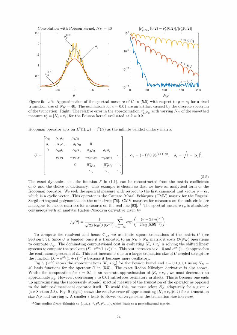
-1 -0.5 0 0.5 1

0

0.5

1

1.5

2

2.5

Convolution with Poisson kernel, NK = 40

θ

ρg

ν0.1g

@@R

ν0.01g

@@R

0 50 100 150 20010

-15

10-10

10-5

100

|νεg,NK (0.2)− νεg(0.2)|/|νεg(0.2)|

NK

ε = 0.01

ε = 0.1

ε = 0.5

Figure 9: Left: Approximation of the spectral measure of U in (5.5) with respect to g = e1 for a fixedtruncation size of NK = 40. The oscillations for ε = 0.01 are an artifact caused by the discrete spectrumof the truncation. Right: The relative error in the approximation νεg,NK with varying NK of the smoothedmeasure νεg = [Kε ∗ νg] for the Poisson kernel evaluated at θ = 0.2.

Koopman operator acts on L2(Ω, ω) = `2(N) as the infinite banded unitary matrix

U =

α0 α1ρ0 ρ1ρ0

ρ0 −α1α0 −ρ1α0 0

0 α2ρ1 −α2α1 α3ρ2 ρ3ρ2

ρ2ρ1 −ρ2α1 −α3α2 −ρ3α2. . .

0 α4ρ3 −α4α3. . .

. . .. . .

. . .

, αj = (−1)j0.95(j+1)/2, ρj =

√1− |αj |2.

(5.5)The exact dynamics, i.e., the function F in (1.1), can be reconstructed from the matrix coefficientsof U and the choice of dictionary. This example is chosen so that we have an analytical form of theKoopman operator. We seek the spectral measure with respect to the first canonical unit vector g = e1,which is a cyclic vector. This operator is the Cantero–Moral–Velazquez (CMV) matrix for the Rogers–Szego orthogonal polynomials on the unit circle [78]. CMV matrices for measures on the unit circle areanalogous to Jacobi matrices for measures on the real line [93].18 The spectral measure νg is absolutelycontinuous with an analytic Radon–Nikodym derivative given by

ρg(θ) =1√

2π log(0.95−1)

∞∑m=−∞

exp

(− (θ − 2πm)2

2 log(0.95−1)

).

To compute the resolvent and hence Cνg , we use finite square truncations of the matrix U (seeSection 5.3). Since U is banded, once it is truncated to an NK ×NK matrix it costs O(NK) operationsto compute Cνg . The dominating computational cost in evaluating [Kε ∗ νg] is solving the shifted linearsystems to compute the resolvent (K−eiθ0(1+ε))−1. This cost increases as ε ↓ 0 and eiθ0(1+ε) approachesthe continuous spectrum of K. This cost increase is due to a larger truncation size of U needed to capturethe function (K − eiθ0(1 + ε))−1g because it becomes more oscillatory.

Fig. 9 (left) shows the approximations [Kε ∗ νg] for the Poisson kernel and ε = 0.1, 0.01 using NK =40 basis functions for the operator U in (5.5). The exact Radon–Nikodym derivative is also shown.Whilst the computation for ε = 0.1 is an accurate approximation of [Kε ∗ νg], we must decrease ε toapproximate ρg. However, decreasing ε to 0.01 introduces oscillatory artifacts. This is because one endsup approximating the (necessarily atomic) spectral measure of the truncation of the operator as opposedto the infinite-dimensional operator itself. To avoid this, we must select NK adaptively for a given ε(see Section 5.3). Fig. 9 (right) shows the relative error of approximating [Kε ∗ νg](0.2) for a truncationsize NK and varying ε. A smaller ε leads to slower convergence as the truncation size increases.

18One applies Gram–Schmidt to 1, z, z−1, z2, z2, . . ., which leads to a pentadiagonal matrix.

24

-1 -0.5 0 0.5 1

0

0.5

1

1.5

2

2.5

Conv. with Poisson kernel, noisy matrix

θ

ρg

ν0.1g

@@R

ν0.01g

@@R

0 50 100 150 20010

-3

10-2

10-1

100

|νεg,NK (0.2)− νεg(0.2)|/|νεg(0.2)| with noisy matrix

NK

ε = 0.01

ε = 0.1

ε = 0.5

Figure 10: Left: Approximation of the spectral measure of U in (5.5) with respect to g = e1 for anadaptive choice of NK but with truncation matrix perturbed by normal random variables of mean 0 andstandard deviation δ = 0.001. The oscillations for ε = 0.01 are an artifact caused by the ill-conditioningof the resolvent as ε ↓ 0. Right: The relative error in the numerical approximation νεg,NK , correspondingto truncation size NK , of the smoothed measure νεg = [Kε ∗ νg] for the Poisson kernel in (3.7) with thesame model of matrix perturbation. The error is averaged over 50 realizations.

Therefore, there is a numerical balancing act. On the one hand, we wish to stay as far away from thespectrum as possible so that the evaluation of [Kε ∗ νg] is computationally cheap. On the other hand, wedesire a good approximation of νg, which requires small ε > 0. The Poisson kernel leads to O(ε log(ε−1))convergence as ε ↓ 0, making it computationally infeasible to compute the spectral measure to more thana few digits of accuracy. High-order kernels allow us to compute spectral measures with better accuracy.

5.1.2 The need for high-order kernels II: A stability tradeoff

Continuing with (5.5), the shifted linear system involved in computing the resolvent operator becomesincreasingly ill-conditioned as ε ↓ 0 when eiθ0 ∈ σ(K). This is because ‖(K − eiθ0(1 + ε))−1‖ = O(ε−1)(see Section 5.2.2). The ResDMD framework developed in Section 4 uses approximations of Galerkintruncations of K with convergence to the exact truncation in the large data limit M1 →∞ as the numberof data points increases (see Section 4.1.3). Therefore, the stability of the resolvent operator is crucialfor data-driven approximations as we have inexact matrix entries.

We now repeat the experiment from Section 5.1.1, but now with an adaptive NK for fixed ε and weperturb each entry of an NK×NK truncation of U with independent Gaussian random variables of mean0 and standard deviation δ = 0.001. Fig. 10 (left) shows the approximation of the spectral measureνg with g = e1. Whilst ε = 0.1 appears stable to the eye, decreasing to ε = 0.01 yields an inaccurateapproximation since ‖(K− eiθ0(1 + ε))−1‖ increases and the shifted linear systems become more sensitiveto noise. Fig. 10 (right) shows the mean error of the approximation of [Kε ∗ νg] over 50 independentrealizations. In contrast to the convergence to machine precision in Fig. 9 (right), the errors in Fig. 10(right) plateau due to the perturbation of the matrix with a larger final error for smaller ε.

The error in approximating νg with a perturbed truncation of the operator is unavoidable but thePoisson kernel is suboptimal in this regard. For a perturbation of order δ, the accuracy achieved by thePoisson kernel scales as O(ε log(ε−1) + δ/ε). Balancing these terms whilst ignoring logarithmic factorsleads to the noise dependent choice ε ∼ δ1/2. This choice yields an overall error scaling ofO(δ1/2 log(δ−1)).High-order kernels can get arbitrarily close to the optimal scaling of O(δ) as δ → 0.

5.1.3 The need for high-order kernels III: Localization of the kernel

We revisit the tent map of Section 3.5.1 with the choice of g given in (3.20). Fig. 11 shows the computedmeasure using the Poisson kernel, where we have chosen NK adaptively to avoid the problem in Sec-tion 5.1.1 and ε = 0.1 so that with M1 = 25 = 32 the error in Section 5.1.2 is negligible. For comparison,we do the same computation but with a 6th order kernel (see Section 5.2.1). As a function, the Poissonkernel decays slowly away from 0, and hence the singular part of the spectral measure at θ = 0 is notlocalized. In contrast, mth order kernels obey a decay condition (see (3.9)) so are more localized for a

25

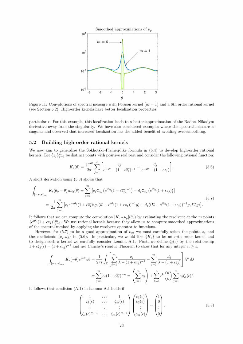
-3 -2 -1 0 1 2 310

-2

10-1

100

101

Smoothed approximations of νg

θ

m = 1

m = 6 -

Figure 11: Convolutions of spectral measure with Poisson kernel (m = 1) and a 6th order rational kernel(see Section 5.2). High-order kernels have better localization properties.

particular ε. For this example, this localization leads to a better approximation of the Radon–Nikodymderivative away from the singularity. We have also considered examples where the spectral measure issingular and observed that increased localization has the added benefit of avoiding over-smoothing.

5.2 Building high-order rational kernels

We now aim to generalize the Sokhotski–Plemelj-like formula in (5.4) to develop high-order rationalkernels. Let zjmj=1 be distinct points with positive real part and consider the following rational function:

Kε(θ) =e−iθ

2π

m∑j=1

[cj

e−iθ − (1 + εzj)−1− dje−iθ − (1 + εzj)

]. (5.6)

A short derivation using (5.3) shows that∫[−π,π]per

Kε(θ0 − θ) dνg(θ) =

m∑j=1

[cjCνg

(eiθ0(1 + εzj)

−1)− djCνg

(eiθ0(1 + εzj)

)]=−1

2π

m∑j=1

[cje−iθ0(1 + εzj)〈g, (K − eiθ0(1 + εzj))

−1g〉+ dj〈(K − eiθ0(1 + εzj))−1g,K∗g〉

].

(5.7)

It follows that we can compute the convolution [Kε ∗ νg](θ0) by evaluating the resolvent at the m pointseiθ0(1 + εzj)mj=1. We use rational kernels because they allow us to compute smoothed approximationsof the spectral method by applying the resolvent operator to functions.

However, for (5.7) to be a good approximation of νg, we must carefully select the points zj andthe coefficients cj , dj in (5.6). In particular, we would like Kε to be an mth order kernel andto design such a kernel we carefully consider Lemma A.1. First, we define ζj(ε) by the relationship1 + εζj(ε) = (1 + εzj)

−1 and use Cauchy’s residue Theorem to show that for any integer n ≥ 1,∫[−π,π]per

Kε(−θ)einθ dθ =1

2πi

∫T

m∑j=1

cjλ− (1 + εzj)−1

−m∑j=1

djλ− (1 + εzj)

λn dλ=

m∑j=1

cj(1 + εzj)−n =

m∑j=1

cj

+

n∑k=1

εk(n

k

) m∑j=1

cjζj(ε)k.

It follows that condition (A.1) in Lemma A.1 holds if1 . . . 1

ζ1(ε) . . . ζm(ε)...

. . ....

ζ1(ε)m−1 . . . ζm(ε)m−1

c1(ε)c2(ε)

...cm(ε)

=

10...0

. (5.8)

26

Note also that, if this holds, the coefficients cj = cj(ε) remain bounded as ε ↓ 0. To ensure that the decaycondition in (A.2) is satisfied, let ω = (e−iθ − 1)/ε, then we have

Kε(θ) =ε−1e−iθ

2π

m∑j=1

[cj

ω − ζj(ε)− djω − zj

]. (5.9)

Therefore, we have

ωKε(θ) =ε−1e−iθ

2π

m∑j=1

[cj +

cjζj(ε)

ω − ζj(ε)− dj −

djzjω − zj

]

=ε−1e−iθ

2π

m∑j=1

(cj − dj) +ε−1e−iθ

2π

m∑j=1

[cjζj(ε)

ω − ζj(ε)− djzjω − zj

].

By repeating essentially the same argument m times, we arrive at the following relationship:

ωmKε(θ) =ε−1e−iθ

2π

m−1∑k=0

ωm−1−km∑j=1

(cjζj(ε)k − djzkj ) +

m∑j=1

(cjζj(ε)

m

ω − ζj(ε)−

djzmj

ω − zj

) . (5.10)

This means that we should select the dk’s so that1 . . . 1z1 . . . zm...

. . ....

zm−11 . . . zm−1

m

d1

d2

...dm

=

10...0

. (5.11)

We conclude that if the coefficients cjmj=1 and djmj=1 satisfy (5.8) and (5.11), then:

m−1∑k=0

ωm−1−km∑j=1

(cjζj(ε)k − djzkj ) = 0,

∣∣∣∣∣∣m∑j=1

(cjζj(ε)

m

ω − ζj(ε)−

djzmj

ω − zj

)∣∣∣∣∣∣ . |ω|−1.

By (5.10), this means that |ω|m |Kε(θ)| . ε−1|ω|−1. Moreover, since |Kε(θ)| . ε−1 we see that |Kε(θ)| .minε−1, εm|θ|−(m+1) . εm(ε+ |θ|)−(m+1). Using Lemma A.1, we have proved the following proposition.

Proposition 5.1. Let zjmj=1 be distinct points with positive real part and let Kε be given by (5.6).Then, Kε is an mth order kernel for [−π, π]per if the coefficients cjmj=1 and djmj=1 satisfy (5.8) and(5.11), respectively.

5.2.1 The choice of rational kernel

We are free to choose the points zjmj=1 in Proposition 5.1 subject to Re(zj) > 0, after which the linearsystems (5.8) and (5.11) provide suitable cjmj=1 (dependent on ε) and djmj=1 (independent of ε). Asa natural extension of the Poisson kernel in (3.7), we select the points zjmj=1 as

zj = 1 +

(2j

m+ 1− 1

)i, 1 ≤ j ≤ m. (5.12)

The kernels that we have developed are typically not real-valued. Since νg is a probability measure andhence real-valued, we often gain better accuracy for a particular ε by considering the kernel Re(Kε) andthis is what we do throughout this paper. The convolution with Re(Kε) can be computed by taking thereal part of the right-hand side of (5.7). The first six kernels with the choice ε = 1 are shown in Fig. 12.The exact coefficients cj , djmj=1 for ε = 0.1 are shown in Table 2 for the first six kernels.

5.2.2 Revisiting the examples in Section 5.1.1 and Section 5.1.2

To demonstrate the advantages of high-order rational kernels, we revisit the operator U given in (5.5)and look again at two of the numerical needs for high-order kernels.

27

-3 -2 -1 0 1 2 3

0

0.5

1

1.5

2

2.5

Re(K1(θ))

θ

m = 1

m = 2 -

m = 3

m = 4 -

m = 5

m = 6 -

Figure 12: The mth-order kernels (5.6) constructed with the choice (5.12) for ε = 1 and 1 ≤ m ≤ 6.

m d1, . . . , ddm/2e c1(ε), . . . , cdm/2e(ε), ε = 0.1

2

1−3i2

3+10i

6

3 −2− i, 5

−202+79i80 , 121

20

4

−39+65i24 , 17−85i

8

−1165710−2944643i750000 , 513570+3570527i

250000

5

15+10i

4 , −39−13i2 , 65

2

4052283−1460282i

648000 , −2393157+486551i81000 , 190333

4000

6

725−1015i

192, −2775+6475i

192, 1073−7511i

96

24883929805+81589072062i

8067360000, −19967590755−93596942182i

1613472000, 7898770397+102424504746i

806736000

Table 2: Coefficients in the rational kernels in (5.6) for 1 ≤ m ≤ 6, the choice (5.12), and ε = 0.1. Wegive the first dm/2e coefficients as cm+1−j = cj and dm+1−j = dj .

• A numerical tradeoff. Fig. 13 (left) shows the convergence of [Kε ∗ νg] for the rational kernels inSection 5.2.1. We see the rates of convergence that are predicted from Theorem 3.1. In practice, thismeans that we rarely need to take ε below 0.01 for very accurate results and often we just take ε = 0.1.

• A stability tradeoff. Let KNK be an NK ×NK truncation of K (see Section 5.3 for how we do this).An important property of our truncations is that ‖KNK‖ ≤ ‖K‖ = 1. Using the standard Neumannseries for the inverse, it follows that any λ such that |λ| > 1 has ‖(KNK−λ)−1‖ ≤ 1/(|λ|−1). In general,this is the best one can hope for. Suppose that instead of KNK , we have access to KNK = KNK+∆ with‖∆‖ ≤ δ. If |λ| = 1+O(ε) > 1+δ, then since ‖KNK‖ ≤ 1+δ we have ‖(KNK −λ)−1‖ ≤ 1/(|λ|−1−δ).Using the second resolvent identity for the first equality, we have a relative error of

‖[(KNK − λ)−1 − (KNK − λ)−1]g‖‖(KNK − λ)−1g‖

=‖[−(KNK − λ)−1∆](KNK − λ)−1g‖

‖(KNK − λ)−1g‖

≤ ‖(KNK − λ)−1∆‖ ≤ δ

|λ| − 1− δ= O(ε−1δ).

Theorems 3.1 and 3.2 show that an mth order kernel provides error rates of O(εm log(ε−1)) as ε→ 0.Therefore, we have an error that is asymptotically of size O(εm log(ε−1)) from using a kernel andO(ε−1δ) from using a perturbed version of KNK . Here, we are assuming that NK is sufficiently largeto render the truncation error negligible. By selecting ε = δ1/(m+1), we balance these two errors andhave an overall error of O(δ

mm+1 log(δ−1)). For large m the convergence rate is close to the optimal

rate of O(δ). In Fig. 13 (right), we show the relative error |νεg(0.2) − ρg(0.2)|/|ρg(0.2)| when usingtruncations where each entry is perturbed by independent normal random variables of mean 0 andstandard deviation δ.19 We have chosen NK sufficiently large and ε ∼ δ1/(m+1). The error is averagedover 50 trials so that we are showing the expected rates of convergence.

19Strictly speaking, the operator norm of this perturbation need not be bounded by δ, but the scaling argument for thechoice ε = δ1/(m+1) remains the same.

28

10-3

10-2

10-1

100

10-15

10-10

10-5

100

|ρg(0.2)− [Kε ∗ νg](0.2)|/|ρg(0.2)|

ε

m = 1

m = 2

m= 3

m=

4

m=

5

m=

6

10-10

10-5

10-10

10-8

10-6

10-4

10-2

100

|ρg(0.2)−[Kε∗νg ](0.2)||ρg(0.2)| with noisy matrix

δ

O(δ12 log(δ

−1 ))

O(δ67

log(δ−1 ))

m = 1

m=

6

Figure 13: Left: The pointwise relative error in smoothed measures of the operator in (5.5) computedusing the high-order kernels in Section 5.2.1 for 1 ≤ m ≤ 6. Right: The pointwise relative error in thecomputed smoothed measure using the perturbed KNK and ε ∼ δ1/(m+1).

5.3 An algorithm for evaluating a smoothed spectral measure

We now seek to evaluate [Kε ∗ νg] at θ1, . . . , θP ∈ [−π, π]per, where Kε is a rational kernel of the form(5.6). This requires the evaluation of (K − λ)−1 for different values of λ (see (5.7)). We first describehow to evaluate [Kε ∗ νg] at a single point θ0 before precomputing a factorization to derive an efficientscheme for evaluating at θ1, . . . , θP .

5.3.1 Evaluating a smoothed spectral measure at a single point

To evaluate [Kε ∗ νg] at a single point θ0 ∈ [−π, π]per we use the setup of ResDMD (see Section 4.1)so that we can obtain rigorous a posteriori error bounds on the computed resolvents, allowing us toadaptively select the dictionary size NK based on the smoothing parameter ε. Since K is an isometry,we only need to compute (K − z)−1 for |z| > 1 = ‖K‖ and so we can achieve our goal with standardGalerkin truncations of K.

Theorem 5.1. Suppose that K is an isometry and λ ∈ C with |λ| > 1. Let ψ1, ψ2, . . . , be a dictionaryof observables and VNK = span ψ1, . . . , ψNK, so that ∪NK∈NVNK is dense in L2(Ω, ω). Then, for anysequence of observables gNK ∈ VNK such that limNK→∞ gNK = g ∈ L2(Ω, ω), we have

limNK→∞

(PVNKKP

∗VNK− λINK

)−1

gNK = (K − λ)−1g,

where PVNK is the orthogonal projection operator onto VNK and INK is the NK ×NK identity matrix.

Proof. Since |λ| > ‖K‖ and ‖PVNKKP∗VNK‖ ≤ ‖K‖, we have the following absolutely convergent Neumann

series: (PVNKKP

∗VNK− λINK

)−1

= − 1

λ

∞∑k=0

1

λk(PVNKKP

∗VNK

)k, (K − λ)−1 = − 1

λ

∞∑k=0

1

λkKk.

Using |λ| > ‖K‖, we can bound the tails of these series uniformly in NK so we just need to show that(PVNKKP

∗VNK

)k converges strongly to Kk for k ≥ 0. This clearly holds for k = 0 and k = 1. For k > 1,

we apply induction using the fact that if a sequence of matrices TNK and SNK converge strongly to Tand S, respectively, then the product TNKSNK converges strongly to the composition T S.

We now apply Theorem 5.1 to evaluate [Kε ∗ νg] at θ0. Recall from (5.7) that there are two types ofinner-products to compute: (i) 〈g, (K−λ)−1g〉 and (ii) 〈(K−λ)−1g,K∗g〉 for some observable g. We forma sequence of observables gNK ∈ VNK by setting gNK = PVNK g, which can be approximately computedfrom snapshot data as

gNK =

NK∑j=1

aaajψj , aaa = (Ψ∗0WΨ0)−1Ψ∗0W

g(xxx

(1)0 )...

g(xxx(M1)0 )

∈ CNK , (5.13)

29

Algorithm 4 A computational framework for evaluating an approximate spectral measure with respectto g ∈ L2(Ω, ω) at θkPk=1 ⊂ [−π, π]per of an isometry K using snapshot data.

Input: Snapshot data xxx(j)0

M1j=1, xxx

(j)1

M1j=1 (such that xxx

(j)1 = F (xxx

(j)0 )), quadrature weights wjM1

j=1,

a dictionary of observables ψjNKj=1, m ∈ N, smoothing parameter 0 < ε < 1 (accuracy goal is εm),distinct points zjmj=1 ⊂ C with Re(zj) > 0 (recommended choice is (5.12)), and evaluation points

θkPk=1 ⊂ [−π, π]per.

1: Solve (5.8) and (5.11) for c1(ε), . . . , cm(ε) ∈ C and d1, . . . , dm ∈ C, respectively.2: Compute Ψ∗0WΨ0 and Ψ∗0WΨ1, where Ψ0 and Ψ1 are given in (4.4).3: Compute a generalized Schur decomposition of Ψ∗0WΨ1 and Ψ∗0WΨ0, i.e., Ψ∗0WΨ1 = QSZ∗ and

Ψ∗0WΨ0 = QTZ∗, where Q,Z are unitary and S, T are upper triangular.4: Compute aaa in (5.13) and v1 = TZ∗aaa, v2 = T ∗Q∗aaa, and v3 = S∗Q∗aaa.5: for k = 1, . . . , P do6: Compute Ij = (S − eiθk(1 + εzj)T )−1v1 for 1 ≤ j ≤ m.7: Compute νεg(θk) = −1

2π

∑mj=1 Re

[cj(ε)e

−iθk(1 + εzj)(I∗j v2) + dj(v

∗3Ij)

].

8: end for

Output: Values of the approximate spectral measure, i.e., νεg(θk)Pk=1.

where Ψ0 and W are given in Section 4.1.1. Under the conditions discussed in Section 4.1.3, we havelimM1→∞ gNK = gNK . Since we have

(PVNKKP

∗VNK− λINK

)−1

gNK = limM1→∞

NK∑j=1

[(Ψ∗0WΨ1 − λΨ∗0WΨ0)−1Ψ∗0WΨ0aaa

]jψj ,

it follows that our two types of inner-products satisfy⟨gNK ,

(PVNKKP

∗VNK− λINK

)−1

gNK

⟩= limM1→∞

aaa∗Ψ∗0WΨ0(Ψ∗0WΨ1 − λ(Ψ∗0WΨ0))−1Ψ∗0WΨ0aaa, (5.14)⟨(PVNKKP

∗VNK− λINK

)−1

gNK ,K∗gNK⟩

= limM1→∞

aaa∗Ψ∗0WΨ1(Ψ∗0WΨ1 − λΨ∗0WΨ0)−1Ψ∗0WΨ0aaa. (5.15)

For a given value of M1, the right-hand side of (5.14) and (5.15) can then be substituted into (5.7) toevaluate [Kε ∗ νg](θ0). Often we can estimate the error between these computed inner-products and thelimiting value as M1 →∞ by comparing the computations for different M1 or by using a priori knowledgeof the convergence rates. In Appendix C, we show how NK can be adaptively chosen (by approximatingthe error in the large data limit and adding observables to the dictionary if required) so that the left-hand sides of (5.14) and (5.15) approximate the inner-products 〈g, (K − λ)−1g〉 and 〈(K − λ)−1g,K∗g〉,respectively, to a desired accuracy. Thus, for a given smoothing parameter ε, we have a principled wayof selecting (a) the sample size M1 and (b) the truncation size NK to ensure that our approximations ofthe inner-products in (5.7) are accurate. In general, the cost of point evaluation of [Kε ∗ νg] using theseformulas is O(N3

K) operations as it requires m solutions of NK ×NK dense linear systems.

5.3.2 Evaluating a smoothed spectral measure at multiple points

To evaluate [Kε ∗ νg] at θ1, . . . , θP ∈ [−π, π]per, one can be more computationally efficient than in-dependently computing each of the inner-products in (5.14) and (5.15) for each θk for 1 ≤ k ≤ P .Instead, one can compute a generalized Schur decomposition and use it to speed up the evaluation. LetΨ∗0WΨ1 = QSZ∗ and Ψ∗0WΨ0 = QTZ∗ be a generalized Schur decomposition, where Q and Z areunitary matrices and S and T are upper-triangular matrices. With this decomposition in hand, we have

aaa∗Ψ∗0WΨ0(Ψ∗0WΨ1 − λ(Ψ∗0WΨ0))−1Ψ∗0WΨ0aaa = aaa∗QT (S − λT )−1TZ∗aaa,

aaa∗Ψ∗0WΨ1(Ψ∗0WΨ1 − λΨ∗0WΨ0)−1Ψ∗0WΨ0aaa = aaa∗QS(S − λT )−1TZ∗aaa.

Now, after computing the generalized Schur decomposition costing O(N3K) operations, each evaluation re-

quires solving NK×NK upper-triangular linear systems in O(N2K) operations. Additional computational

savings can be realized if one is willing to do each evaluation at θ1, . . . , θP in parallel. We summarize theevaluation scheme in Algorithm 4.

30

θ1

θ2

`

`

-3 -2 -1 0 1 2 3

0

0.2

0.4

0.6

0.8

1

1.2

1.4

g = C1eix1e−(x2

3+x24)/2

θ-3 -2 -1 0 1 2 3

0

0.1

0.2

0.3

0.4

0.5

0.6

0.7

0.8

g = C2eix2e−(x2

3+x24)/2

θ

-3 -2 -1 0 1 2 3

0.1

0.12

0.14

0.16

0.18

0.2

0.22

0.24

g = C3x3e−(x2

3+x24)/2

θ-3 -2 -1 0 1 2 3

0.05

0.1

0.15

0.2

0.25

0.3

0.35

0.4

g = C4x4e−(x2

3+x24)/2

θ

Figure 14: Left: Physical setup of the double pendulum. Right: Computed spectral measures for fourobservables g. The constants Cj are normalization factors so that ‖g‖ = 1.

5.4 Numerical example: The double pendulum

The double pendulum is shown in Fig. 14 (left) and is a physical system that exhibits rich dynamicbehavior. It is chaotic and governed by the following system of ordinary differential equations [57]:

θ1 =2p1 − 3p2 cos(θ1 − θ2)

16− 9 cos2(θ1 − θ2), θ2 =

8p2 − 3p1 cos(θ1 − θ2)

16− 9 cos2(θ1 − θ2),

p1 = −3(θ1θ2 sin(θ1 − θ2) + sin(θ1)

), p2 = −3

(−θ1θ2 sin(θ1 − θ2) +

1

3sin(θ2)

),

where p1 = 8θ1 + 3θ2 cos(θ1− θ2)) and p2 = 2θ2 + 3θ1 cos(θ1− θ2)). We take both pendula to be of equallength ` and mass M , with units M`2 = 6 and G/` = 1/3 for simplicity, where G is the gravitationalconstant. Our state-space is the four-dimensional space xxx = (θ1, θ2, p1, p2) in Ω = [−π, π]2per × R2.We consider the Koopman operator corresponding to discrete time-steps with ∆t = 1. The system isHamiltonian and hence K is unitary on L2(Ω, ω) with the usual Lebesgue measure.

To compute the resolvent, we use Algorithm 4 with a dictionary consisting of tensor-products of theFourier basis in x1 and x2, and Hermite functions in x3 and x4, together with an ordering correspondingto a hyperbolic cross approximation. We simulate the dynamics using the ode45 command in MATLABfor a single time-step on an equispaced grid and use the trapezoidal rule. The chaotic nature of thedynamical system is not a problem as we only collect trajectory data with M2 = 1 (i.e., snapshot data).Following the procedure outlined in Section 5.3, the maximum value of M1 used in this example is1,562,500 and the maximum value of NK used is 2528.

Fig. 14 (right) shows spectral measures for four observables computed using the 6th order kernel inTable 2 with ε = 0.1. The results are verified against the 6th order kernel with smaller ε and a larger NK .We also show the results for the Poisson kernel (m = 1), which produces an over-smoothed estimate of νg.The Fourier observables (top row) display a pronounced peak at θ = 0 and quite flat spectral measuresaway from zero. In contrast, the Hermite observables (bottom row) display no peak at θ = 0 and abroader spectral measure away from zero. These observables have a richer interplay with the dynamics,and their spectral measures are more spread out over the spectrum of the Koopman operator.

6 High-dimensional dynamical systems

In the numerical examples of Sections 4 and 5, the dimension of the state-space of (1.1) is modest so thatwe can write down a dictionary. However, for larger dimensions that arise in applications such as fluiddynamics, molecular dynamics, and climate forecasting, it is not possible to explicitly store a dictionary.

31

DMD is a popular approach to studying Koopman operators associated with high-dimensional dynamics,which can yield accurate results for periodic or quasiperiodic systems but is often unable to adequatelycapture relevant nonlinear dynamics [6, 19,110] as it implicitly seeks to fit linear dynamics. Moreover, arigorous connection with Galerkin approximations of Koopman operators does not always hold [105].

When d is large, we are naturally in the setting of NK M1 as a sufficiently rich dictionary mustbe selected. In other words, the dimension of the dictionary subspace is usually much larger than thesnapshot data when d is large. How can we approximate spectral properties of K when d is largeand NK M1? This section extends our algorithms to high dimensions and provides applications tomolecular dynamics and the study of noise leakage of turbulent flow past a cascade of airfoils.

6.1 Adapting our algorithms to use data-driven dictionaries

Our main idea to tackle large d is to construct a data-driven dictionary using the so-called kernel trick.

6.1.1 Kernelized EDMD

A naive construction of the matrix Ψ∗0WΨ1 in Section 4.1.1 requiresO(N2KM1) operations, which becomes

impractical when NK is large. Kernelized EDMD [111] aims to make EDMD practical for large NK . The

idea is to compute a much smaller matrix KEDMD that has a subset of the same eigenvalues as KEDMD.

Proposition 6.1 (Proposition 1 of [111] with additional weight matrix). Let√WΨ0 = UΣV ∗ be a

SVD, where U ∈ CM1×M1 is a unitary matrix, Σ ∈ CM1×M1 is a diagonal matrix with non-increasingnon-negative entries, and V ∈ CNK×M1 is an isometry. Define the M1 ×M1 matrix

KEDMD = (Σ†U∗)(√WΨ1Ψ∗0

√W )(UΣ†),

where ‘†’ is the pseudoinverse. Then, for some λ 6= 0 and v ∈ CM1 , (λ, v) is an eigenvalue-eigenvector

pair of KEDMD if and only if (λ, V v) is an eigenvalue-eigenvector pair of KEDMD.

Suitable matrices U and Σ in Proposition 6.1 can be recovered from the eigenvalue decomposition√WΨ0Ψ∗0

√W = UΣ2U∗. Moreover, both matrices

√WΨ0Ψ∗0

√W ∈ CM1×M1 and

√WΨ1Ψ∗0

√W ∈

CM1×M1 can be computed using inner-products:

[√WΨ0Ψ∗0

√W ]jk =

√wjΨ(xxx

(j)0 )Ψ(xxx

(k)0 )∗√wk, [

√WΨ1Ψ∗0

√W ]jk =

√wjΨ(xxx

(j)1 )Ψ(xxx

(k)0 )∗√wk, (6.1)

where we recall that Ψ(xxx) is a row vector of the dictionary evaluated at xxx.20 Kernelized EDMD appliesthe kernel trick to compute the inner-products in (6.1) in an implicitly defined reproducing Hilbert spaceH with inner-product 〈·, ·〉H [84]. A positive-definite kernel function S : Ω×Ω→ R induces a feature mapϕ : Rd → H so that 〈ϕ(xxx), ϕ(yyy)〉H = S(xxx,yyy). This leads to a choice of dictionary (or reweighted featuremap) Ψ(xxx) so that Ψ(xxx)Ψ(yyy)∗ = 〈ϕ(xxx), ϕ(yyy)〉H = S(xxx,yyy). Often S can be evaluated in O(d) operations,

so that the matrices√WΨ0Ψ∗0

√W and

√WΨ1Ψ∗0

√W can be computed in O(dM2

1 ) operations. KEDMD

can thus be constructed in O(dM21 ) operations, a considerable saving, with a significant reduction in

memory consumption.As a naive first attempt at extending our algorithms in this manner, one could consider Algorithm 2

with kernelized EDMD. The residual for a vector v ∈ CM1 becomes

v∗[(Ψ1V )∗W (Ψ1V )− λ(Ψ1V )∗W (Ψ0V )− λ(Ψ0V )∗W (Ψ1V ) + |λ|2(Ψ0V )∗W (Ψ0V )]v

v∗(Ψ0V )∗W (Ψ0V )v∗. (6.2)

Unfortunately, the following simple proposition shows that the residual in (6.2) always vanishes. Thisshould be interpreted as over-fitting of the snapshot data when NK ≥M1.

Proposition 6.2. Suppose that NK ≥ M1 and√WΨ0 has rank M1 (independent columns). For any

eigenvalue-eigenvector pair λ and v ∈ CM1 of KEDMD, the residual in (6.2) vanishes.

Proof. The numerator in (6.2) is the square of the `2-vector norm of√W (Ψ1 − λΨ0)V v. From the

decomposition√WΨ0 = UΣV ∗, we have√W (Ψ1 − λΨ0)V v =

√WΨ1V v − λUΣv =

√WΨ1Ψ∗0

√WUΣ+v − λUΣv.

Since Σ is invertible, we must have that√WΨ1Ψ∗0

√WUΣ+ = UΣKEDMD. It follows that

√W (Ψ1 −

λΨ0)V v = UΣ(KEDMD − λ)v = 0.

20This is the transpose of the convention in [111].

32

In other words, the restriction NK ≥ M1 prevents the large data convergence (M1 → ∞) of Algo-rithm 2 for fixed NK . Note that even if this were not the case, the residual in (6.2) may not fit into theL2(Ω, ω) Galerkin framework due to the implicit reproducing Hilbert space. A way to overcome theseissues is to consider two sets of snapshot data (see Section 6.1.2).

6.1.2 Kernelized versions of the algorithms

Kernelized EDMD computes the eigenvalues, eigenvectors and corresponding Koopman modes of KEDMD.The required operations to compute these quantities are inner-products and hence can be computed byevaluating S. In particular, the kth eigenfunction ψk corresponding to eigenvector vk ∈ CM1 of KEDMD

can be evaluated as [111, Remark 8]

ψk(xxx) =[S(xxx,xxx

(1)0 ) S(xxx,xxx

(2)0 ) · · · S(xxx,xxx

(M1)0 )

](UΣ+)vk, k = 1, . . . ,M1. (6.3)

This leads to the simple kernelization of our algorithms summarized in Algorithm 5. The idea is a

two-step process: (1) We use kernelized EDMD with a data set xxx(j)0 ,xxx

(j)1

M ′1j=1 to compute a dictionary

corresponding to the dominant eigenfunctions of KEDMD and (2) We apply our algorithms using this

dictionary on another set yyy(j)0 , yyy

(j)1

M ′′1j=1 of snapshot data. Of course, there are many algorithmic details

regarding the choice of kernel, the second set of snapshot data, and how to a posteriori check that thelearned dictionary is suitable. We describe these details now:

• Choice of kernel: The choice of kernel S determines the dictionary and the best choice depends onthe application. In the following experiments, we use the Gaussian radial basis function kernel

S(xxx,yyy) = exp(−γ‖xxx− yyy‖2

), (6.4)

where we select γ to be the squared reciprocal of the average `2-norm of the snapshot data after it isshifted to have mean zero.

• Regularization: The matrix√WΨ0Ψ∗0

√W can be ill-conditioned [10] so we always regularize and

consider√WΨ0Ψ∗0

√W + η‖

√WΨ0Ψ∗0

√W‖ for small η. This is common practice in DMD.

• Acquiring a second set of snapshot data: Given snapshot data with random and independent ini-

tial conditions, one can simply split the snapshot data up into two parts so that we have xxx(j)0 ,xxx

(j)1

M ′1j=1

and yyy(j)0 , yyy

(j)1

M ′′1j=1, where M1 = M ′1 + M ′′1 . For initial conditions that are distributed according to a

quadrature rule, if one already has access to M ′1 snapshots then one must typically go back to the orig-inal dynamical system and request M ′′1 further snapshots. In both cases, we denote the total amountof snapshot data as M1 = M ′1 +M ′′1 . The first set of M ′1 snapshots is used in the kernelized approachto refine a large initial dictionary of size N ′K (implicitly defined by the chosen kernel) to a smallerdata-driven one of size N ′′K , while the second set of M ′′1 snapshots are used to apply our ResDMDalgorithms. We recommend that M ′′1 ≥M ′1.

• Selecting the second dictionary: We start with a large dictionary of size N ′K and apply a kernelizedapproach to construct a second dictionary of size N ′′K . To construct the second dictionary, we computethe dominant N ′′K eigenvectors of KEDMD that hopefully capture the most important dynamics. In this

paper, we compute a complete eigendecomposition of KEDMD; however, for problems with extremelylarge M ′1, iterative methods are recommended to compute these dominant eigenvectors.

• Rigorous results: It is well-known that the eigenvalues computed by kernel EDMD may suffer fromspectral pollution. In our setting, we do not directly use kernel EDMD to compute eigenvalues of K.Instead, we are only using kernel EDMD to select a reasonable dictionary of size N ′′K , after which ourrigorous algorithms can be used (see Algorithms 2 to 4, with convergence as M ′′1 →∞).

• A posteriori check of the second dictionary: We use yyy(j)0 , yyy

(j)1

M ′′1j=1 to check the quality of the

constructed second dictionary. By studying the residuals and using the error control in Theorem B.1,we can tell a posteriori whether the second dictionary is satisfactory and whether N ′′K is sufficientlylarge.

33

Algorithm 5 A computational framework for kernelized versions of Algorithms 2 to 4.

Input: Snapshot data xxx(j)0 ,xxx

(j)1

M ′1j=1 and yyy(j)

0 , yyy(j)1

M ′′1j=1, positive-definite kernel function S : Ω×Ω→ R,

and positive integer N ′′K ≤M ′1.

1: Apply kernel EDMD to xxx(j)0 ,xxx

(j)1

M ′1j=1 with kernel S to compute the matrices

√WΨ0Ψ∗0

√W and√

WΨ1Ψ∗0√W using (6.1) and the kernel trick.

2: Compute U and Σ from the eigendecomposition√WΨ0Ψ∗0

√W = UΣ2U∗.

3: Compute the dominant N ′′K eigenvectors of KEDMD = (Σ†U∗)√WΨ1Ψ∗0

√W (UΣ†) and stack them

column-by-column into Z ∈ CM ′1×N ′′K .4: Apply a QR decomposition to orthogonalize Z to Q =

[Q1 · · · QN ′′K

]∈ CM ′1×N ′′K .

5: Apply Algorithms 2 to 4 with yyy(j)0 , yyy

(j)1

M ′′1j=1 and the dictionary ψj

N ′′Kj=1, where

ψj(xxx) =[S(xxx,xxx

(1)0 ) S(xxx,xxx

(2)0 ) · · · S(xxx,xxx

(M ′1)0 )

](UΣ+)Qj , 1 ≤ j ≤ N ′′K .

Output: Spectral properties of Koopman operator according to Algorithms 2 to 4.

6.2 Example: MD simulation of the Adenylate Kinase enzyme (d = 20,046)

Molecular dynamics (MD) analyzes the movement of atoms and molecules by numerically solving New-ton’s equations of motion for a system of interacting particles. Energies and forces between particles aretypically computed using potentials. MD is arguably one of the most robust approaches for simulatingmacromolecular dynamics, in large part due to the availability of full atomistic detail [28]. Recently,DMD-type and Koopman techniques are making an impact in MD [48, 69, 85, 86]. For example, [50]applies kernel EDMD to the positions of the carbon atoms in an n-butane (d = 12) and shows that theEDMD eigenfunctions parameterize a dihedral angle that controls key dynamics.

Here, we study trajectory data from the dynamics of Adenylate Kinase (ADK), which is an enzyme(see Fig. 15) that catalyzes important phosphate reactions in cellular biology [36]. ADK is a commonbenchmark enzyme in MD [87] and consists of 3341 atoms split into 214 residues (specific monomersthat can be thought of as parts). The trajectory data comes from an all-atom equilibrium simulation for1.004 × 10−6s with a so-called CHARMM force field that is produced on PSC Anton [89] and publiclyavailable [8]. The data consists of a single trajectory of the positions of all atoms as ADK moves. Tomake the system Hamiltonian, we append the data with approximations of the velocities computed usingcentered finite differences. This leads to d = 6×3341 = 20046. We vertically stack the data (as discussedin Section 4) and sample the trajectory data every 240× 10−12s so that M1 = 4184 and M2 = 1.

To apply the kernelized version of Algorithm 4, we subselect M ′1 = 2000 initial conditions fromthe trajectory data and used the Gaussian radial basis function kernel in (6.4). We select N ′′K = 1000EDMD eigenfunctions and append the dictionary with the four observables of interest (discussed below).Accuracy of the corresponding matrices in (4.7) is verified by comparing to smallerM ′′1 and also computingpseudospectra with Algorithm 3.

ADK has three parts of its molecule called CORE, LID, and NMP (see Fig. 15 (left)). The LID andNMP domains move around the stable CORE. By computing root-mean-square-fluctuations, we selectthe most mobile residue from the LID and NMP domains. These residues have canonical dihedral angles(φ, ψ) defined on the backbone atoms [75] that determine the overall shape of the residue. Fig. 15 (middle,left) shows the spectral measures with respect to these dihedral angles (where we have subtracted themean angle value) for both selected residues. These spectral measures are computed using the sixthorder rational kernel with ε = 0.1 (see Table 2). The computed spectral measures are verified with higherorder kernels and smaller ε, as well as comparison with a polynomial kernel instead of a Gaussian radialbasis function kernel. The spectral measures for the angles in the LID residue are much broader thanfor the NMP residue. This hints at a more complicated dynamical interaction and may have biologicalconsequences. We hope that this example can be a catalyze for the use of spectral measures in MD.

6.3 Example: Turbulent flow past a cascade of aerofoils (d = 295,122)

One of the most successful applications of DMD is in fluid dynamics [23,27,65,79,101]. Here, we consider alarge-scale wall-resolved turbulent flow past a periodic cascade of aerofoils with a stagger angle 56.9 and aone-sided tip gap. The setup is motivated by the need to reduce noise sources from flying objects [72]. Weuse a high-fidelity simulation that solves the fully non-linear Navier–Stokes equations [51] with Reynolds

34

@@@

residues

LID

CORE

@@NMP

-3 -2 -1 0 1 2 3

0.14

0.16

0.18

0.2

0.22

0.24

0.26

θ

LID

φ

ψ

AAAAU

-3 -2 -1 0 1 2 3

0

0.1

0.2

0.3

0.4

0.5

0.6

θ

NMP

φ@@@I

ψ

Figure 15: Left: Structure of ADK which has three domains: CORE (green), LID (yellow) and NMP(red). Middle and right: Spectral measures with respect to the dihedral angles of the selected residues.

number 3.88×105 and Mach number 0.07. The data consists of a 2D slice of the pressure field, measuredat 295,122 points, for trajectories of length 798 that are sampled every 2× 10−5s. We stack the data inthe form of (4.1) so that M1 = 797 and M2 = 2.

To apply the kernelized version of Algorithm 2, we subselect M ′1 = 350 initial conditions from thetrajectory data and used the Gaussian radial basis function kernel in (6.4). We select N ′′K = 250 EDMDeigenfunctions as our dictionary. Accuracy of the corresponding matrices in (4.7) is verified by comparingto smaller M ′′1 and also computing pseudospectra with Algorithm 3.

Fig. 16 shows the computed Koopman modes for a range of representative frequencies. We have alsoshown the corresponding Koopman modes computed using DMD. In the case of DMD and ResDMD,each mode is only defined up to a global phase. Moreover, the color maps for each λ differ because ofthe pressure modulus variations with frequency. For the first row of Fig. 16, ResDMD shows strongeracoustic waves between the cascades. Detecting these vibrations is important as they can be damaging toturbines in engines [71]. For the second and third row of Fig. 16, ResDMD shows larger scale turbulentfluctuations past the trailing edge corresponding to the right of the figure. This can be crucial forunderstanding acoustic interactions with nearby structures such as subsequent blade rows [112]. For thethird row, DMD shows a clear acoustic source just above the wing. This source is less distinct in thecase of ResDMD due to nonlinear interference. The residuals for ResDMD are also shown and are smallgiven the huge state-space dimension. This example demonstrates two benefits of the kernelized versionof ResDMD (see Algorithms 2 and 3) compared with DMD: (1) ResDMD can capture the nonlineardynamics, and (2) It computes residuals as well, thus providing an accuracy certificate.

Acknowledgements

The first author is supported by a Research Fellowship at Trinity College, Cambridge, and a FoundationSciences Mathematiques de Paris postdoctoral fellowship at Ecole Normale Superieure. The work of thesecond author is supported by the National Science Foundation grants DMS-1818757, DMS-1952757 andDMS-2045646. The authors are grateful to Andrew Horning for reading a draft of this manuscript.

A A useful criterion for mth order kernels

The following lemma is used to prove Proposition 3.1 and also to build mth order rational kernels of theform (5.6). It provides sufficient conditions for a family of integrable functions to be an mth order kernel.

Lemma A.1. Let Kε : ε ∈ (0, 1] be a family of integrable functions on the periodic interval [−π, π]per

that integrate to 1. Suppose that there exists a constant C such that for any integer n with 0 < n ≤ m−1,∣∣∣∣∣∫

[−π,π]per

Kε(−θ)einθdθ − 1

∣∣∣∣∣ ≤ Cεm log(ε−1), (A.1)

and such that

|Kε(θ)| ≤Cεm

(ε+ |θ|)m+1. (A.2)

for any θ ∈ [−π, π]per and ε ∈ (0, 1]. Then Kε is an mth order kernel for [−π, π]per.

35

DMD ResDMD, res = 0.0054λ

=e0.1

1i

acoustic vibrations

DMD ResDMD, res = 0.0128

λ=e0.5

1i

turbulentfluctuations

DMD ResDMD, res = 0.0196

λ=e0.7

1i

acoustic source

Figure 16: Left column: Modes computed by DMD. Right column: Modes computed by ResDMD withcomputed residuals. Each row corresponds to the different values of λ that correspond to certain physicalfrequency of noise pollution.

36

Proof of Lemma A.1. There are three properties that an mth order kernel must satisfy (see Defini-tion 3.1). Properties (i) and (iii) are already assumed in the statement of the Lemma. To show part (ii)of Definition 3.1, let n be an integer and consider θn with n < m. We use the convergent power seriesfor the principal branch of the logarithm around 1 to write, for θ ∈ [−π/4, π/4],

θn =

∞∑k=1

ak,n(eiθ − 1)k =

m−1∑k=1

ak,n(eiθ − 1)k︸ ︷︷ ︸=pn,m(θ)

+θm(eiθ − 1)m

θm

∞∑k=m

ak,n(eiθ − 1)k−m︸ ︷︷ ︸=hn,m(θ)

,

where ak,n ∈ C and the domain of the trigonometric polynomial pn,m is extended to [−π, π]per. Wenote that hn,m(θ) is a bounded continuous function on [−π/4, π/4]. Since |

∫[−π,π]per

Kε(−θ)pn,m(θ)dθ−pn,m(0)| . εm log(ε−1), we know by (A.2) that∣∣∣∣∣

∫ π/4

−π/4θnKε(−θ) dθ

∣∣∣∣∣ .∫ π/(4ε)

0

εmτm

(1 + τ)m+1dτ +

∫|θ|>π/4|Kε(−θ)||pn,m(θ)| dθ + εm log(ε−1)

. εm log(ε−1) +

∫|θ|>π/4

εm‖pn,m‖L∞(ε+ π/4)m+1

dθ . εm log(ε−1).

Furthermore, by (A.2) we obtain∣∣∣∣∣∫

[−π,−π/4)∪(π/4,π]

θnKε(−θ) dθ

∣∣∣∣∣ ≤ πn(2π − π/2)Cεm

(ε+ π/4)m+1. εm.

Property (ii) of Definition 3.1 now follows by the symmetry of (3.8) under the mapping θ 7→ −θ.

B ResDMD for computing spectra and pseudospectra

In this section, we show how to modify ResDMD in Section 4.2 to rigorously compute the global spectralproperties of the Koopman operator K. Throughout this section, we make the following assumptionabout the dictionary ψjNKj=1:

Assumption: spanψ ∈ VNK : NK ∈ N forms a core of K.

This assumption means that the closure of the restriction of K to spanψ ∈ VNK : NK ∈ N is K. Inother words, the assumption allows us to study the infinite-dimensional operator K, which acts on apossibly strict subdomain D(K) ⊂ L2(Ω, ω), by considering its action on the observables in VNK . Thisis vital for capturing the full operator K, and hence, equivalently, the full dynamics. To simplify ourarguments, we also assume that ψj is independent of NK for a fixed j, and that VNK ⊂ VNK+1. Theselast two assumptions can be dropped with minor modifications to our arguments.

We begin by re-writing the quantity ‖(K − λ)−1‖−1 as a minimal residual. Given a linear operatorT with domain D(T ), we define the injection modulus J (T ) = inf‖Tψ‖ : ‖ψ‖ = 1, ψ ∈ D(T ). It iswell-known that

‖(K − λ)−1‖−1 = minJ (K − λ),J (K∗ − λ) ≤ J (K − λ) = infg∈D(K),g 6=0

‖(K − λ)g‖‖g‖

,

with equality if λ /∈ σ(K). Therefore σ(K) = λ : minJ (K − λ),J (K∗ − λ) = 0.

B.1 The metric space

Before discussing the convergence of Algorithm 3, we must be precise about what we mean by convergence.A reliable algorithm for computing a spectral set should converge locally on compact subsets of C. Inother words, it should converge to the full spectral set and have no limiting points that are not in thespectral set. We see that our algorithms achieve this, and we use the following metric space to quantifythis convergence.

In general, σ(K) is a closed and possibly unbounded subset of C. We therefore use the Attouch–Wetsmetric defined by [9]

dAW(C1, C2) =

∞∑n=1

2−n min

1, sup|x|≤n

|dist(x,C1)− dist(x,C2)|, (B.1)

37

where C1, C2 ∈ Cl(C) and Cl(C) is the set of closed non-empty21 subsets of C. This generalizes thefamiliar Hausdorff metric on compact sets to unbounded closed sets, and corresponds to local uniformconverge on compact subsets of C. In the case that the spectral set is bounded, the two topologies andnotions of convergence agree. An intuitive characterization of the Attouch–Wets topology, that we usein our proofs, is as follows. For any closed non-empty sets C and Cn, dAW(Cn, C)→ 0 if and only if forany δ > 0 and Bm(0) (closed ball of radius m ∈ N about 0), there exists N such that if n > N thenCn ∩Bm(0) ⊂ C +Bδ(0) and C ∩Bm(0) ⊂ Cn +Bδ(0).

B.2 Computing the approximate point pseudospectra

We first compute the approximate point pseudospectrum, which is given by

σε,ap(K) := cl (λ ∈ C : J (K − λ) < ε) . (B.2)

In other words, σε,ap(K) is the closure of the set of all λ such that there exists g ∈ D(K) of norm 1with ‖(K − λ)g‖ < ε. Such an observable g is known as an (ε-)approximate eigenfunction. Moreover,σε(K) = σε,ap(K) ∪

λ : λ ∈ σp(K∗)

. Thus σε,ap(K) is equivalent to the usual pseudospectrum σε(K),

up to the eigenvalues of K∗. In most cases of interest, we have σε,ap(K) = σε(K).To compute σε,ap(K), we begin by providing approximations of the function λ 7→ J (K− λ) using the

residual in (4.6). The following lemma shows how to do this.

Lemma B.1. Define a relative residual as

τM1,NK (λ,K) = minggg∈CNK

√√√√∑NKj,k=1 gjgk

[(Ψ∗1WΨ1)jk − λ(Ψ∗1WΨ0)jk − λ(Ψ∗0WΨ1)jk + |λ|2(Ψ∗0WΨ0)jk

]∑NKj,k=1 gjgk(Ψ∗0WΨ0)jk

.

(B.3)Then, assuming (4.7) holds, we have

limM1→∞

τM1,NK (λ,K) = τNK (λ,K) := ming∈VNK

√√√√∫Ω |[Kg](xxx)− λg(xxx)|2 dω(xxx)∫Ω|g(xxx)|2 dω(xxx)

. (B.4)

Moreover, τNK (λ,K) is a non-increasing function of NK and converges uniformly down to J (K− λ) oncompact subsets of C as a function of the spectral parameter λ.

Proof. The limit (B.4) follows trivially from the convergence of matrices in (4.7). Since VNK ⊂ VNK+1,we must have that τNK (λ,K) is a non-increasing function of NK . By definition, we also have thatτNK (λ,K) ≥ J (K − λ) for every λ and NK . Now let 0 < ε < 1 and choose g ∈ D(K) of norm 1 suchthat ‖(K − λ)g‖ ≤ J (K − λ) + ε. Since spanψ ∈ VNK : NK ∈ N forms a core of K, there exists somen and gn ∈ Vn such that ‖(K − λ)gn‖ ≤ ‖(K − λ)g‖ + ε and ‖g − gn‖ ≤ ε. We find that ‖gn‖ ≥ 1 − εand hence that τn(λ,K) ≤ (J (K − λ) + 2ε)/(1− ε). Since this holds for any 0 < ε < 1, we must havelimNK→∞ τNK (λ,K) = J (K − λ). Since J (K − λ) is Lipschitz continuous in λ and hence continuous,we have that τNK (λ,K) converges uniformly down to J (K − λ) on compact subsets of C by Dini’sTheorem.

In other words, in the large data limit, we can compute τNK (λ,K), which is at least as large asJ (K−λ), and converges uniformly as our truncations parameter NK increases. To compute τM1,NK (λ,K),one can first diagonalize Ψ∗0WΨ0 to compute a regularized (Ψ∗0WΨ0)−1/2 and then the problem reducesto computing a standard singular value decomposition. To turn τNK (λ,K) into an approximation ofσε,ap(K), we search for points where this function is less than ε. Suppose that Grid(NK) is a sequence offinite grids such that for any λ ∈ C, limNK→∞ dist(λ,Grid(NK)) = 0. For example, we could take

Grid(NK) =1

NK[Z + iZ] ∩ z ∈ C : |z| ≤ NK. (B.5)

In practice, one considers a grid of points over the region of interest in the complex plane. We then define

ΓεNK (K) := λ ∈ Grid(NK) : τNK (λ,K) < ε .21We can add the empty set as an isolated point of this metric space to cover the case that σ(K) may be empty. In what

follows, this is implicitly done in our algorithms since the output is eventually the empty set in such circumstances.

38

Our full algorithm is summarized in Algorithm 3. Note that due to the nature of the non-linear pencil in(B.3), one cannot use decompositions such as the generalized Schur decomposition (used in Algorithm 4)to speed up computations.

We can now state our convergence theorem, which says that the output of Algorithm 3 lies in σε,ap(K)and converges to σε,ap(K) as M1 →∞.

Theorem B.1. Let ε > 0. Then, ΓεNK (K) ⊂ σε,ap(K) and

limNK→∞

dAW

(ΓεNK (K), σε,ap(K)

)= 0. (B.6)

In other words, we recover the full approximate point pseudospectrum without spectral pollution.

Proof. If λ ∈ ΓεNK (K), then J (K − λ) ≤ τNK (λ,K) < ε by Lemma B.1. It follows that ΓεNK (K) ⊂σε,ap(K). Now suppose that σε,ap(K) 6= ∅. It follows that there exists λ ∈ C with J (K − λ) < ε.Since J (K − λ) is continuous in λ and limNK→∞ dist(λ,Grid(NK)) = 0, it follows that ΓεNK (K) 6= ∅for large NK . We use the characterization of the Attouch–Wets topology. Suppose that m is large suchthat Bm(0) ∩ σε,ap(K) 6= ∅. Since ΓεNK (K) ⊂ σε,ap(K), we clearly have ΓεNK (K) ∩ Bm(0) ⊂ σε,ap(K).Hence, to prove (B.6), we must show that given δ > 0, there exists n0 such that if NK > n0 thenσε,ap(K) ∩ Bm(0) ⊂ ΓεNK (K) +Bδ(0). Suppose for a contradiction that this statement is false. Then,there exists δ > 0, λnj ∈ σε,ap(K) ∩ Bm(0), and nj → ∞ such that dist(λnj ,Γ

εnj (K)) ≥ δ. Without loss

of generality, we can assume that λnj → λ ∈ σε,ap(K) ∩ Bm(0). There exists some z with J (K − z) < εand |λ− z| ≤ δ/2. Let znj ∈ Grid(nj) such that |z − znj | ≤ dist(z,Grid(nj)) + nj

−1. Note that we musthave limnj→∞ |z − znj | = 0. We then have

τnj (znj ,K) ≤∣∣τnj (znj ,K)− J (K − znj )

∣∣+∣∣J (K − z)− J (K − znj )

∣∣+ J (K − z)︸ ︷︷ ︸<ε

. (B.7)

But, J (K − λ) is continuous in λ and τnj converges uniformly to J (K − ·) on compact subsets of C byLemma B.1. It follows that the first two terms on the right-hand side of (B.7) must converge to zero.Hence for large nj , we have τnj (znj ,K) < ε so that znj ∈ Γεnj (K). But

∣∣znj − λ∣∣ ≤ |z − λ|+ ∣∣znj − z∣∣ ≤δ/2 + |z − znj |, which is smaller than δ for large nj , and we reach the desired contradiction.

Theorem B.1 is stated for an algorithm that uses τNK . Strictly speaking, τNK is only computed asM1 → ∞ (see Lemma B.1). In practice, this is not an issue since we can often estimate the accuracyof the quadrature rule for the computed inner-products by either using known rates of convergence asM1 →∞ (see Section 4.1.3) or comparing answers for different values of M1. We can then combine theseestimates and adaptively select M1 based on NK so that τNK is sufficiently accurate. For example, if τNKis approximated to accuracyO(N−1

K ) by τNK we can set ΓεNK (K) = λ ∈ Grid(NK) : τNK (λ,K)+N−1/2K <

ε, where the N−1/2K term is to ensure that it eventually dominates the quadrature error.

B.3 Recovering the full spectrum and pseudospectrum

In this subsection, we make the following additional assumption:

Assumption: spanψ ∈ VNK : NK ∈ N forms a core of K∗.

If we have access to the matrix elements 〈K∗ψj ,K∗ψi〉, then we can apply the techniques describedin Section 4 to compute τNK (λ,K∗) in the large data limit M1 →∞. Define

ΓεNK (K) =λ ∈ Grid(NK) : minτNK (λ,K), τNK (λ,K∗) < ε

.

The proof of Theorem B.1 can be adapted to show that ΓεNK (K) ⊂ σε(K) as well as the convergence

limNK→∞ dAW(ΓεNK (K), σε(K)) = 0. Unfortunately, in general, one does not have access to approxima-tions of 〈K∗ψj ,K∗ψi〉. Nevertheless, one can overcome this.

To compute σε(K), we note that due to Theorem B.1, it is enough to compute σε,ap(K∗) since σε(K) =σε,ap(K) ∪ λ : λ ∈ σε,ap(K∗). Let N1, N2 ∈ N, with N1 ≥ N2, and consider the matrices Ψ0 and Ψ1

computed using N1 dictionary functions. Assume that (4.7) holds and let

LN1(λ) = limM1→∞

Ψ∗0WΨ1(Ψ∗0WΨ0)−1Ψ∗1WΨ0 − λΨ∗1WΨ0 − λΨ∗0WΨ1 + |λ|2Ψ∗0WΨ0 ∈ CN1×N1 .

39

Note that this matrix can be obtained from the given data in the large data limit M1 → ∞. Let PSdenote the orthogonal projection onto a subspace S ⊂ L2(Ω, ω). If g =

∑N2

j=1 ψjgj ∈ VN2, then a simple

but tedious computation shows that

⟨PVN1

(K∗ − λ)g,PVN1(K∗ − λ)g

⟩=

N2∑j,k=1

gjgk[LN1(λ)]jk. (B.8)

In other words, this inner-product is given by a squareN2×N2 truncation of the matrix LN1(λ) ∈ CN1×N1 .

The following lemma uses the fact that (B.8) provides an increasingly more accurate approximation ofthe inner-product

⟨(K∗ − λ)g, (K∗ − λ)g

⟩, as N1 →∞.

Lemma B.2. Define υN1,N2(λ,K) = ming∈VN2

,‖g‖=1

√∑N2

j,k=1 gjgk[LN1(λ)]jk. Then, υN1,N2

(λ,K) is anon-decreasing function of N1 and, for fixed N2, converges uniformly up to τN2

(λ,K∗) on compact subsetsof C as a function of λ as N1 →∞.

Proof. It is clear that υN1,N2(λ,K) is a non-decreasing function of N1. Since PVN1strongly converges to

the identity and (K∗−λ)P∗VN2acts on a finite-dimensional subspace, we also have that limN1→∞ ‖(PVN1

−I)(K∗ − λ)P∗VN2

‖ = 0. The uniform convergence of υN1,N2(λ,K) up to τN2(λ,K∗) on compact subsets of

C now follows from Dini’s theorem.

We have the following statement that shows we have inclusion and convergence.

Theorem B.2. Let ε > 0 and define ΓεN2,N1(K) = λ ∈ Grid(N2) : υN1,N2

(λ,K) + 1/N2 ≤ ε. ThenlimN1→∞ ΓεN2,N1

(K) = ΓεN2(K) =

λ ∈ Grid(N2) : τN2(λ,K∗) + 1/N2 ≤ ε

=: ΓεN2

(K). Moreover, we

have ΓεN2(K) ⊂ σε,ap(K∗) and limN2→∞ dAW(ΓεN2

(K),λ : λ ∈ σε,ap(K∗)

) = 0.

Proof. We prove that ΓεN2(K) = limN1→∞ ΓεN2,N1

(K) exists and is given by the set ΓεN2(K) in the state-

ment of the theorem. The rest of the proof carries over from Theorem B.1 and its proof with minormodifications. (The additional term N−1

2 is needed to ensure convergence to the pseudospectrum in the

second limit - it is added so that we can use “≤” instead of “<” in the definition of ΓεN2,N1to ensure the

existence of the first limit via the following argument.) Fix λ ∈ Grid(N2). If τN2(λ,K∗) +N−12 ≤ ε, then

by Lemma B.2, υN1,N2(λ,K) +N−1

2 ≤ ε. It follows that ΓεN2(K) ⊂ ΓεN2,N1

(K). If τN2(λ,K∗) +N−1

2 > ε,

then since limN1→∞ υN1,N2(λ,K) = τN2

(λ,K∗), we must have υN1,N2(λ,K) +N−1

2 > ε for large N1. Thetheorem now follows.

Combining Theorem B.1 and Theorem B.2, we have the following theorem that shows how the fullspectrum and pseudospectrum can be recovered.

Corollary B.1. For any ε > 0, we have

limN2→∞

limN1→∞

[ΓεN2

(K) ∪ ΓεN2,N1(K)]

= σε(K).

Additionally, we have

limε↓0

limN2→∞

limN1→∞

[ΓεN2

(K) ∪ ΓεN2,N1(K)]

= σ(K),

where the convergence holds in the Attouch–Wets topology.

C Computation of rational kernel convolutions with error con-trol

In this section, we show that the required convolutions with rational kernels can be computed rigorouslywith error control. Recall from (5.7) that there are two types of inner-products that we need to compute:(i) 〈g, (K − λ)−1g〉, and (ii) 〈(K − λ)−1g,K∗g〉 for some observable g. Here, we show that the inner-products can be computed with error control via the left-hand sides of (5.14) and (5.15), by adaptivelyselecting the truncations size NK for a fixed smoothing parameter ε. Without loss of generality, we

40

assume that g is normalized so that ‖g‖ = 1 and we denote gNK = Ψaaa. To compute the error bounds inthe large data limit, we also use the fact that

hNK =

NK∑j=1

[(Ψ∗0WΨ1 − λΨ∗0WΨ0)−1Ψ∗0WΨ0aaa

]jψj = Ψhhh ≈ (PVNKP∗VN − λIN )−1gNK .

The following theorem shows that we can bound the error of using the left-hand sides of (5.14) and (5.15)to approximate the desired inner-products.

Theorem C.1. Let λ ∈ C with |λ| > 1. Consider the setup of Section 5.3 with ‖g‖ = 1 and de-fine δ1(NK) = ‖g − gNK‖, δ2(NK) = ‖(K − λ)(PVNKKP

∗VNK

− λINK )−1gNK − gNK‖, and δ3(NK) =

‖(PVNKKP∗VNK− λINK )−1gNK‖. Then, limNK→∞ δ1(NK) = limNK→∞ δ2(NK) = 0 and δ3(NK) remains

bounded as NK →∞. Moreover, we have∣∣∣⟨gNK , (PVNKKP∗VNK − λINK )−1gNK

⟩−⟨g, (K − λ)−1g

⟩∣∣∣ ≤ δ1(NK) + δ2(NK)

|λ| − 1+ δ1(NK)δ3(NK),∣∣∣⟨(PVNKKP

∗VNK− λINK )−1gNK ,K∗gNK

⟩−⟨(K − λ)−1g,K∗g

⟩∣∣∣ ≤ δ1(NK) + δ2(NK)

|λ| − 1+ δ1(NK)δ3(NK).

Assuming (4.7), δ2(NK) and δ3(NK) can be computed in the large data limit via

δ2(NK)2 = limM1→∞

hhh∗Ψ∗0WΨ0hhh · res(λ, hNK )2 − 2Re(aaa∗(Ψ∗0WΨ1 − λΨ∗0WΨ0)hhh

)+ aaa∗Ψ∗0WΨ0aaa, (C.1)

δ3(NK)2 = limM1→∞

hhh∗Ψ∗0WΨ0hhh. (C.2)

Proof. First, by assumption, we have limNK→∞ δ1(NK) = 0. Using this, together with Theorem 5.1 andthe fact that K is bounded, we must have limNK→∞ δ2(NK) = 0. Similarly we must have that δ3(NK)remains bounded as NK →∞. Since |λ| > 1 and ‖K‖ = 1, it follows from the arguments concerning thenumerical range in Section 5.2.2 that ‖(K − λ)−1‖ ≤ 1/(|λ| − 1). It follows that

‖(PVNKKP∗VNK− λINK )−1gNK − (K − λ)−1g‖ ≤

‖(K − λ)(PVNKKP∗VNK− λINK )−1gNK − g‖

|λ| − 1

≤‖(K − λ)(PVNKKP

∗VNK− λINK )−1gNK − gNK‖+ ‖g − gNK‖|λ| − 1

≤ δ1(NK) + δ2(NK)

|λ| − 1.

We now re-write the following inner-product⟨gNK , (PVNKKP

∗VNK− λINK )−1gNK

⟩=⟨g, (K − λ)−1g

⟩+ 〈gNK − g, (PVNKKP

∗VNK− λINK )−1gNK 〉

+⟨g, (PVNKKP

∗VNK− λINK )−1gNK − (K − λ)−1g

⟩.

Since ‖g‖ = 1, it follows by the Cauchy–Schwarz inequality that∣∣∣⟨gNK , (PVNKKP∗VNK − λINK )−1gNK

⟩−⟨g, (K − λ)−1g

⟩∣∣∣ ≤ δ1(NK) + δ2(NK)

|λ| − 1

+ δ1(NK)∥∥∥(PVNKKP

∗VNK− λINK )−1gNK

∥∥∥ .Similarly, since ‖K∗‖ ≤ 1, we obtain∣∣∣⟨(PVNKKP

∗VNK− λINK )−1gNK ,K∗gNK

⟩−⟨(K − λ)−1g,K∗g

⟩∣∣∣ ≤ δ1(NK) + δ2(NK)

|λ| − 1

+ δ1(NK)∥∥∥(PVNKKP

∗VNK− λINK )−1gNK

∥∥∥ .This proves the upper bounds in the theorem. The equalities in (C.1) and (C.2) follow from expandingthe inner-products and from the definition of hhh.

From Theorem C.1, we see that if δ1(NK) is known, then we can compute the inner-products〈g, (K − λ)−1g〉 and 〈(K − λ)−1g,K∗g〉 to any desired accuracy by adaptively selecting NK . More-over, the error bounds in Theorem C.1 can be computed in O(N2

K) operations without the generalizedSchur decomposition. In practice, we increase NK , keeping track of the computed inner-product, untilconvergence is apparent.

41

References

[1] B. Adcock and A. C. Hansen. Stable reconstructions in Hilbert spaces and the resolution of the Gibbsphenomenon. Appl. Comput. Harm. Anal., 32(3):357–388, 2012.

[2] H. Arbabi and I. Mezic. Ergodic theory, dynamic mode decomposition, and computation of spectral prop-erties of the Koopman operator. SIAM J. Appl. Dyn. Syst., 16(4):2096–2126, 2017.

[3] H. Arbabi and I. Mezic. Study of dynamics in post-transient flows using Koopman mode decomposition.Phys. Rev. Fluids, 2(12):124402, 2017.

[4] V. I. Arnold. Mathematical Methods of Classical Mechanics. Springer-Verlag, New York,, 1989.

[5] V. I. Arnold and A. Avez. Ergodic Problems of Classical Mechanics, volume 9. New York, Benjamin, 1968.

[6] P. J. Baddoo, B. Herrmann, B. J. McKeon, and S. L. Brunton. Kernel learning for robust dynamicmode decomposition: Linear and nonlinear disambiguation optimization (LANDO). arXiv preprintarXiv:2106.01510, 2021.

[7] J. Basley, L. Pastur, F. Lusseyran, T. M. Faure, and N. Delprat. Experimental investigation of globalstructures in an incompressible cavity flow using time-resolved PIV. Experiments in Fluids, 50(4):905–918,2011.

[8] O. Beckstein, S. Fan, R. J. Gowers, M. Matta, and L. Wang. AdK equilibrium dataset. https://www.mdanalysis.org/MDAnalysisData/adk_equilibrium.html.

[9] G. Beer. Topologies on Closed and Closed Convex Sets, volume 268. Springer Science & Business Media,1993.

[10] M. Belkin. Approximation beats concentration? An approximation view on inference with smooth radialkernels. In Conference On Learning Theory, pages 1348–1361. PMLR, 2018.

[11] P. Benner, S. Gugercin, and K. Willcox. A survey of projection-based model reduction methods for para-metric dynamical systems. SIAM Rev., 57(4):483–531, 2015.

[12] E. Berger, M. Sastuba, D. Vogt, B. Jung, and H. Ben Amor. Estimation of perturbations in robotic behaviorusing dynamic mode decomposition. Adv. Robot., 29(5):331–343, 2015.

[13] P. Billingsley. Convergence of Probability Measures. John Wiley & Sons, second edition, 1999.

[14] G. D. Birkhoff. Proof of the ergodic theorem. Proc. Nat. Acad. Sci., 17(12):656–660, 1931.

[15] A. Bottcher and B. Silbermann. The finite section method for Toeplitz operators on the quarter-plane withpiecewise continuous symbols. Mathematische Nachrichten, 110(1):279–291, 1983.

[16] D. Bruder, B. Gillespie, C. D. Remy, and R. Vasudevan. Modeling and control of soft robots using theKoopman operator and model predictive control. arXiv preprint arXiv:1902.02827, 2019.

[17] B. W. Brunton, L. A. Johnson, J. G. Ojemann, and J. N. Kutz. Extracting spatial–temporal coherentpatterns in large-scale neural recordings using dynamic mode decomposition. J. Neuro. Meth., 258:1–15,2016.

[18] S. L. Brunton, B. W. Brunton, J. L. Proctor, E. Kaiser, and J. N. Kutz. Chaos as an intermittently forcedlinear system. Nature Commun., 8(1):1–9, 2017.

[19] S. L. Brunton, B. W. Brunton, J. L. Proctor, and J. N. Kutz. Koopman invariant subspaces and finitelinear representations of nonlinear dynamical systems for control. PloS one, 11(2):e0150171, 2016.

[20] S. L. Brunton, M. Budisic, E. Kaiser, and J. N. Kutz. Modern Koopman theory for dynamical systems.arXiv preprint arXiv:2102.12086, 2021.

[21] S. L. Brunton and J. N. Kutz. Data-driven science and engineering: Machine learning, dynamical systems,and control. Cambridge University Press, 2019.

[22] S. L. Brunton, J. L. Proctor, and J. N. Kutz. Discovering governing equations from data by sparse identi-fication of nonlinear dynamical systems. Proc. Nat. Acad. Sci., 113(15):3932–3937, 2016.

[23] M. Budisic, R. Mohr, and I. Mezic. Applied Koopmanism. Chaos, 22(4):047510, 2012.

[24] H.-J. Bungartz and M. Griebel. Sparse grids. Acta Numer., 13:147–269, 2004.

[25] D. Burov, D. Giannakis, K. Manohar, and A. Stuart. Kernel analog forecasting: Multiscale test problems.Multi. Model. Sim., 19(2):1011–1040, 2021.

[26] R. E. Caflisch. Monte Carlo and quasi-Monte Carlo methods. Acta Numer., 7:1–49, 1998.

[27] K. K. Chen, J. H. Tu, and C. W. Rowley. Variants of dynamic mode decomposition: boundary condition,Koopman, and Fourier analyses. J. Nonl. Sci., 22(6):887–915, 2012.

[28] R. O. Dror, R. M. Dirks, J. Grossman, H. Xu, and D. E. Shaw. Biomolecular simulation: a computationalmicroscope for molecular biology. Ann. Rev. Biophys., 41:429–452, 2012.

[29] B. A. Dubrovin, A. T. Fomenko, and S. P. Novikov. Modern Geometry — Methods and Applications PartI. The Geometry of Surfaces, Transformation Groups, and Fields, volume 104. Springer Science & BusinessMedia, 21984.

[30] D. Dung, V. Temlyakov, and T. Ullrich. Hyperbolic Cross Approximation. Springer, 2018.

[31] E. S. Epstein. Stochastic dynamic prediction. Tellus, 21(6):739–759, 1969.

42

[32] L. Fejer. Sur les fonctions bornees et integrables. C.R. Acad. Sci. Paris, pages 984–987, 1900.

[33] M. Ghil, M. Allen, M. Dettinger, K. Ide, D. Kondrashov, M. Mann, A. W. Robertson, A. Saunders, Y. Tian,F. Varadi, et al. Advanced spectral methods for climatic time series. Rev. Geophys., 40(1):3–1, 2002.

[34] D. Giannakis. Data-driven spectral decomposition and forecasting of ergodic dynamical systems. Appl.Comput. Harm. Anal., 47(2):338–396, 2019.

[35] D. Giannakis, A. Henriksen, J. A. Tropp, and R. Ward. Learning to forecast dynamical systems fromstreaming data. arXiv preprint arXiv:2109.09703, 2021.

[36] R. N. Goldberg, Y. B. Tewari, and T. N. Bhat. Thermodynamics of enzyme-catalyzed reactions—a databasefor quantitative biochemistry. Bioinfo., 20(16):2874–2877, 2004.

[37] D. Gottlieb and C.-W. Shu. On the Gibbs phenomenon and its resolution. SIAM Rev., 39(4):644–668, 1997.

[38] M. Guo and J. S. Hesthaven. Data-driven reduced order modeling for time-dependent problems. Comput.Meth. Appl. Mech. Eng., 345:75–99, 2019.

[39] P. R. Halmos. Lectures on Ergodic Theory. Courier Dover Publications, 2017.

[40] T. Hastie, R. Tibshirani, and J. Friedman. The Elements of Statistical Learning. Springer-Verlag, 2009.

[41] J. S. Hesthaven. Numerical Methods for Conservation Laws: From Analysis to Algorithms. SIAM, 2017.

[42] A. J. Hey, S. Tansley, K. M. Tolle, et al. The fourth paradigm: data-intensive scientific discovery, volume 1.Microsoft research Redmond, WA, 2009.

[43] R. C. Hilborn et al. Chaos and Nonlinear Dynamics: An Introduction for Scientists and Engineers. OxfordUniversity Press, 2nd edition, 2004.

[44] A. G. Kachurovskii. The rate of convergence in ergodic theorems. Russian Math. Sur., 51(4):653–703, 1996.

[45] E. Kaiser, J. N. Kutz, and S. L. Brunton. Data-driven discovery of Koopman eigenfunctions for control.arXiv preprint arXiv:1707.01146, 2017.

[46] R. E. Kalman. Mathematical description of linear dynamical systems. J. Soc. Ind. Appl. Math., 1(2):152–192, 1963.

[47] Y. Katznelson. An Introduction to Harmonic Analysis. Cambridge University Press, 2004.

[48] S. Klus, F. Nuske, P. Koltai, H. Wu, I. Kevrekidis, C. Schutte, and F. Noe. Data-driven model reductionand transfer operator approximation. J. Nonlin. Sci., 28(3):985–1010, 2018.

[49] S. Klus, F. Nuske, S. Peitz, J.-H. Niemann, C. Clementi, and C. Schutte. Data-driven approximationof the Koopman generator: Model reduction, system identification, and control. Phys. D: Nonl. Pheno.,406:132416, 2020.

[50] S. Klus, I. Schuster, and K. Muandet. Eigendecompositions of transfer operators in reproducing kernelHilbert spaces. J. Nonlin. Sci., 30(1):283–315, 2020.

[51] R. Koch, M. Sanjose, and S. Moreau. Large-eddy simulation of a linear compressor cascade with tip gap:Aerodynamic and acoustic analysis. In AIAA AVIATION 2021 FORUM, page 2312, 2021.

[52] B. Koopman and J. v. Neumann. Dynamical systems of continuous spectra. Proc. Nat. Acad. Sci. USA,18(3):255, 1932.

[53] B. O. Koopman. Hamiltonian systems and transformation in Hilbert space. Proc. Nat. Acad. Sci. USA,17(5):315, 1931.

[54] M. Korda and I. Mezic. On convergence of extended dynamic mode decomposition to the Koopman operator.J. Nonlin. Sci., 28(2):687–710, 2018.

[55] M. Korda, M. Putinar, and I. Mezic. Data-driven spectral analysis of the Koopman operator. Appl. Comput.Harm. Anal., 48(2):599–629, 2020.

[56] J. N. Kutz, S. L. Brunton, B. W. Brunton, and J. L. Proctor. Dynamic mode decomposition: data-drivenmodeling of complex systems. SIAM, 2016.

[57] R. Levien and S. Tan. Double pendulum: An experiment in chaos. Amer. J. Phys., 61(11):1038–1044, 1993.

[58] M. Lewin and E. Sere. Spectral pollution and how to avoid it. Proc. London Math. Soc., 100(3):864–900,2010.

[59] Q. Li, F. Dietrich, E. M. Bollt, and I. G. Kevrekidis. Extended dynamic mode decomposition with dictionarylearning: A data-driven adaptive spectral decomposition of the Koopman operator. Chaos, 27(10):103111,2017.

[60] E. N. Lorenz. Deterministic nonperiodic flow. J. Atmo. Sci., 20(2):130–141, 1963.

[61] B. Lusch, J. N. Kutz, and S. L. Brunton. Deep learning for universal linear embeddings of nonlineardynamics. Nature Commun., 9(1):1–10, 2018.

[62] J. Mann and J. N. Kutz. Dynamic mode decomposition for financial trading strategies. Quant. Finance,16(11):1643–1655, 2016.

[63] A. Mardt, L. Pasquali, H. Wu, and F. Noe. VAMPnets for deep learning of molecular kinetics. NatureCommun., 9(1):1–11, 2018.

[64] I. Mezic. Spectral properties of dynamical systems, model reduction and decompositions. Nonlin. Dyn.,41(1):309–325, 2005.

43

[65] I. Mezic. Analysis of fluid flows via spectral properties of the Koopman operator. Ann. Rev. Fluid Mech.,45:357–378, 2013.

[66] M. Mohri, A. Rostamizadeh, and A. Talwalkar. Foundations of Machine Learning. MIT press, 2018.

[67] S. Moon, B.-S. Han, J. Park, J. M. Seo, and J.-J. Baik. Periodicity and chaos of high-order Lorenz systems.Inter. J. Bifur. Chaos, 27(11):1750176, 2017.

[68] B. S. Nagy, C. Foias, H. Bercovici, and L. Kerchy. Harmonic analysis of operators on Hilbert space. SpringerScience & Business Media, 2010.

[69] F. Nuske, B. G. Keller, G. Perez-Hernandez, A. S. Mey, and F. Noe. Variational approach to molecularkinetics. J. Chem. Theory Comput., 10(4):1739–1752, 2014.

[70] S. E. Otto and C. W. Rowley. Linearly recurrent autoencoder networks for learning dynamics. SIAM J.Appl. Dyn. Syst., 18(1):558–593, 2019.

[71] R. Parker. Acoustic resonances and blade vibration in axial flow compressors. J. Sound Vibr., 92(4):529–539,1984.

[72] N. Peake and A. B. Parry. Modern challenges facing turbomachinery aeroacoustics. Ann. Rev. Fluid Mech.,44:227–248, 2012.

[73] H. Poincare. Les methodes nouvelles de la mecanique celeste, volume 3. Gauthier-Villars, 1899.

[74] J. L. Proctor and P. A. Eckhoff. Discovering dynamic patterns from infectious disease data using dynamicmode decomposition. International Health, 7(2):139–145, 2015.

[75] G. Ramachandran, C. Ramakrishnan, and V. Sasisekharan. Stereochemistry of polypeptide chain configu-rations. J. Mole. Bio., 7(1):95–99, 1963.

[76] M. Reed and B. Simon. Methods of Modern Mathematical Physics. I. Academic Press, New York, secondedition, 1980.

[77] S. Roch and B. Silbermann. C∗-algebra techniques in numerical analysis. J. Oper. Theory, pages 241–280,1996.

[78] L. J. Rogers. Second memoir on the expansion of certain infinite products. Proc. Lond. Math. Soc., 25:318–343, 1893/94.

[79] C. W. Rowley, I. Mezic, S. Bagheri, P. Schlatter, and D. S. Henningson. Spectral analysis of nonlinearflows. J. Fluid Mech., 641:115–127, 2009.

[80] S. H. Rudy, S. L. Brunton, J. L. Proctor, and J. N. Kutz. Data-driven discovery of partial differentialequations. Sci. Adv., 3(4):e1602614, 2017.

[81] B. Saltzman. Finite amplitude free convection as an initial value problem - I. J. Atmo. Sci., 19(4):329–341,1962.

[82] P. J. Schmid. Dynamic mode decomposition of numerical and experimental data. J. Fluid Mech., 656:5–28,2010.

[83] M. Schmidt and H. Lipson. Distilling free-form natural laws from experimental data. science, 324(5923):81–85, 2009.

[84] B. Scholkopf. The kernel trick for distances. Adv. Neur. Info. Proc. Syst., pages 301–307, 2001.

[85] C. R. Schwantes and V. S. Pande. Improvements in Markov state model construction reveal many non-nativeinteractions in the folding of NTL9. J. Chem. Theory Comput., 9(4):2000–2009, 2013.

[86] C. R. Schwantes and V. S. Pande. Modeling molecular kinetics with tICA and the kernel trick. J. Chem.Theory Comput., 11(2):600–608, 2015.

[87] S. L. Seyler and O. Beckstein. Sampling large conformational transitions: Adenylate Kinase as a testingground. Mole. Sim., 40(10-11):855–877, 2014.

[88] E. Shargorodsky. On the level sets of the resolvent norm of a linear operator. Bull. Lon. Math. Soc.,40(3):493–504, 2008.

[89] D. E. Shaw, R. O. Dror, J. K. Salmon, J. Grossman, K. M. Mackenzie, J. A. Bank, C. Young, M. M.Deneroff, B. Batson, K. J. Bowers, et al. Millisecond-scale molecular dynamics simulations on Anton. InProceedings of the conference on high performance computing networking, storage and analysis, pages 1–11,2009.

[90] B.-W. Shen. Nonlinear feedback in a five-dimensional Lorenz model. J. Atmo. Sci., 71(5):1701–1723, 2014.

[91] B.-W. Shen. Nonlinear feedback in a six-dimensional Lorenz model: impact of an additional heating term.Nonlin. Proc. Geophys., 22(6):749–764, 2015.

[92] P. C. Shields. The Theory of Bernoulli Shifts. University of Chicago Press, Chicago, 1973.

[93] B. Simon. CMV matrices: Five years after. J. Comput. Appl. Math., 208(1):120–154, 2007.

[94] C. S. Stefan Klus, Peter Koltai. On the numerical approximation of the Perron-Frobenius and Koopmanoperator. J. Comput. Dyn., 3(1):51–79, 2016.

[95] E. M. Stein and R. Shakarchi. Real Analysis: Measure Theory, Integration, and Hilbert Spaces. PrincetonUniversity Press, 2009.

[96] G. W. Stewart and J.-g. Sun. Matrix perturbation theory. Academic Press, New York, 1990.

44

[97] A. Stuart and A. R. Humphries. Dynamical Systems and Numerical Analysis, volume 2. CambridgeUniversity Press, 1998.

[98] Y. Susuki and I. Mezic. Nonlinear Koopman modes and coherency identification of coupled swing dynamics.IEEE Transactions on Power Systems, 26(4):1894–1904, 2011.

[99] Y. Susuki, I. Mezic, and T. Hikihara. Coherent swing instability of power grids. J. Nonlin. Sci., 21(3):403–439, 2011.

[100] E. Tadmor. Filters, mollifiers and the computation of the Gibbs phenomenon. Acta Numer., 16:305–378,2007.

[101] K. Taira, S. L. Brunton, S. T. Dawson, C. W. Rowley, T. Colonius, B. J. McKeon, O. T. Schmidt,S. Gordeyev, V. Theofilis, and L. S. Ukeiley. Modal analysis of fluid flows: An overview. AIAA J.,55(12):4013–4041, 2017.

[102] L. N. Trefethen and M. Embree. Spectra and Pseudospectra: The Behavior of Nonnormal Matrices andOperators. Princeton University Press, 2005.

[103] L. N. Trefethen, A. E. Trefethen, S. C. Reddy, and T. A. Driscoll. Hydrodynamic stability without eigen-values. Science, 261(5121):578–584, 1993.

[104] L. N. Trefethen and J. Weideman. The exponentially convergent trapezoidal rule. SIAM Review, 56(3):385–458, 2014.

[105] J. H. Tu, C. W. Rowley, D. M. Luchtenburg, S. L. Brunton, and J. N. Kutz. On dynamic mode decompo-sition: Theory and applications. J. Comput. Dyn., 1(2):391–421, 2014.

[106] H. Vandeven. Family of spectral filters for discontinuous problems. J. Sci. Comput., 6(2):159–192, 1991.

[107] P. Walters. An introduction to Ergodic Theory, volume 79. Springer Science & Business Media, 2000.

[108] E. Wegert. Visual Complex Functions: An Introduction with Phase Portraits. Springer Science & BusinessMedia, 2012.

[109] P. Welch. The use of fast Fourier transform for the estimation of power spectra: a method based on timeaveraging over short, modified periodograms. IEEE Trans. Audio Electro., 15(2):70–73, 1967.

[110] M. O. Williams, I. G. Kevrekidis, and C. W. Rowley. A data–driven approximation of the Koopmanoperator: Extending dynamic mode decomposition. J. Nonlin. Sci., 25(6):1307–1346, 2015.

[111] M. O. Williams, C. W. Rowley, and I. G. Kevrekidis. A kernel-based method for data-driven Koopmanspectral analysis. J. Comput. Dyn., 2(2):247, 2015.

[112] B. Woodley and N. Peake. Resonant acoustic frequencies of a tandem cascade. Part 2. Rotating blade rows.J. Fluid Mech., 393:241–256, 1999.

[113] E. Yeung, S. Kundu, and N. Hodas. Learning deep neural network representations for Koopman operatorsof nonlinear dynamical systems. In 2019 American Control Conference (ACC), pages 4832–4839. IEEE,2019.

[114] G. M. Zaslavsky. Chaos, fractional kinetics, and anomalous transport. Phys. Reports, 371(6):461–580, 2002.

[115] Z. Zhao and D. Giannakis. Analog forecasting with dynamics-adapted kernels. Nonlin., 29(9):2888, 2016.

45