Matter and measure - Chem1

Matter and measureA Chem1 Reference Text

Stephen K. Lower • Simon Fraser University

Part 1: Units and dimensions . . . . . . . . . . . . . . . . . . . . . . . . . . . . . . . . . . . . . . . . . . . . . 2Scales and units . . . . . . . . . . . . . . . . . . . . . . . . . . . . . . . . . . . . . . . . . . . . . . . . . . . . . 2

The SI base units . . . . . . . . . . . . . . . . . . . . . . . . . . . . . . . . . . . . . . . . . . . . . . . . . . . . 3

The SI decimal prefixes . . . . . . . . . . . . . . . . . . . . . . . . . . . . . . . . . . . . . . . . . . . . . . . 4

Units outside the SI . . . . . . . . . . . . . . . . . . . . . . . . . . . . . . . . . . . . . . . . . . . . . . . . . . 4

Derived units and dimensions . . . . . . . . . . . . . . . . . . . . . . . . . . . . . . . . . . . . . . . . . . 4

Units and their ranges in Chemistry . . . . . . . . . . . . . . . . . . . . . . . . . . . . . . . . . . . . . 6

Part 2: The meaning of measure: accuracy and precision . . . . . . . . . . . . . . . . . . . . . 11Error in measured values . . . . . . . . . . . . . . . . . . . . . . . . . . . . . . . . . . . . . . . . . . . . . . 11

More than one answer: scatter in measured values. . . . . . . . . . . . . . . . . . . . . . . . . . 12

Dealing with scatter: the mean . . . . . . . . . . . . . . . . . . . . . . . . . . . . . . . . . . . . . . . . . 13

Accuracy and precision . . . . . . . . . . . . . . . . . . . . . . . . . . . . . . . . . . . . . . . . . . . . . . . 13

Absolute and relative uncertainty . . . . . . . . . . . . . . . . . . . . . . . . . . . . . . . . . . . . . . . 15

Part 3: Significant figures and rounding off . . . . . . . . . . . . . . . . . . . . . . . . . . . . . . . . 16Digits, significant and otherwise . . . . . . . . . . . . . . . . . . . . . . . . . . . . . . . . . . . . . . . . 16

Rules for rounding off . . . . . . . . . . . . . . . . . . . . . . . . . . . . . . . . . . . . . . . . . . . . . . . . 17

Rounding off the results of calculations. . . . . . . . . . . . . . . . . . . . . . . . . . . . . . . . . . . 19

Part 4: Assessing the reliability of measurements: simple statistics . . . . . . . . . . . . . 21Attributes of a measurement . . . . . . . . . . . . . . . . . . . . . . . . . . . . . . . . . . . . . . . . . . . 21

Dispersion of the mean . . . . . . . . . . . . . . . . . . . . . . . . . . . . . . . . . . . . . . . . . . . . . . . 22

Systematic error . . . . . . . . . . . . . . . . . . . . . . . . . . . . . . . . . . . . . . . . . . . . . . . . . . . . . 23

Putting statistics to work: assessing reliability . . . . . . . . . . . . . . . . . . . . . . . . . . . . . 24

The bell-shaped curve . . . . . . . . . . . . . . . . . . . . . . . . . . . . . . . . . . . . . . . . . . . . . . . . 25

Confidence intervals . . . . . . . . . . . . . . . . . . . . . . . . . . . . . . . . . . . . . . . . . . . . . . . . . 26

Small data sets. . . . . . . . . . . . . . . . . . . . . . . . . . . . . . . . . . . . . . . . . . . . . . . . . . . . . . 27

Using statistical tests to make decisions . . . . . . . . . . . . . . . . . . . . . . . . . . . . . . . . . . 28

How to lie with statistics: some dangerous pitfalls . . . . . . . . . . . . . . . . . . . . . . . . . . 30

Part 5:

A Web version of this document is available at

http://www.sfu.ca/person/lower/TUTORIALS/matmeas/

1 • Units and dimensionsHave you ever estimated a distance by “stepping it off”— that is, by counting the number of steps required to take you a certain distance? Or perhaps you have used the width of your hand, or the distance from your elbow to a fingertip to compare two dimensions. If so, you have engaged in what is probably the first kind of measurement ever undertaken by primi-tive mankind.

An even more primitive kind of measure would have been that of time. Even a dog knows when its walk or its dinner is due, and all animals whose habitat exposes them to the 24-hour day/night (diurnal) cycle possess an inner clock that synchronizes their mental and metabolic activities to this cycle.

1.1 Scales and unitsThe results of a measurement are always expressed on some kind of a scale that is defined in terms of a particular kind of unit. The first scales of distance were likely related to the human body, either directly (the length of a limb) or indirectly (the distance a man could walk in a day). As civilization developed, a wide variety of measuring scales came into exist-ence, many for the same quantity (such as length), but adapted to particular activities or trades. Eventually, it became apparent that in order for trade and commerce to be possible, these scales had to be defined in terms of standards that would allow measures to be veri-fied, and, when expressed in different units (bushels and pecks, for example), to be corre-lated or converted.

Over the centuries, hundreds of measurement units and scales have developed in the many civilizations that achieved some literate means of recording them. Some, such as those used by the Aztecs, fell out of use and were largely forgotten as these civilizations died out.Other units, such as the various systems of measurement that developed in England, achieved prominence through extension of the Empire and widespread trade.

The most influential event in the history of measurement was undoubtedly the French Rev-olution and the Age of Rationality that followed. This led directly to the metric system that attempted to do away with the confusing multiplicity of measurement scales by reducing them to a few fundamental ones that could be combined in order to express any kind of quantity. The metric system spread rapidly over much of the world, and eventually even to England and the rest of the U.K. when that country established closer economic ties with Europe in the latter part of the 20th Century. The United States is presently the only major country in which “metrication” has made little progress within its own society, probably because of its relative geographical isolation and its vibrant internal economy.

Science, being a truly international endeavor, adopted metric measurement very early on; engineering and related technologies have been slower to make this change, but are gradu-ally doing so. Even the within the metric system, however, a variety of units were employed to measure the same fundamental quantity; for example, energy could be expressed within the metric system in units of ergs, electron-volts, joules, and two kinds of calories. This led, in the mid-1960s, to the adoption of a more basic set of units, the Systeme Internationale (SI) units that are now recognized as the standard for science and, increasingly, for technology of all kinds

Matter and measure

1.2 The SI base unitsIn principle, any physical quantity can be expressed in terms of only seven base units:

Each of these units is defined by a standard which is described in the NIST Web site.

A few special points are worth noting:• ;The base unit of mass is unique in that a decimal prefix (see below) is built-in to it; that is, it is

not the gram, as you might expect.

• ;The base unit of time is the only one that is not metric. Numerous attempts to make it so have never garnered any success; we are still stuck with the 24:60:60 system that we inherited from ancient times. (The ancient Egyptians of around 1500 BC invented the 12-hour day, and the 60:60 part is a remnant of the base-60 system that the Sumerians used for their astronomical calculations around 100 BC.)

• ;Although the number is not explicitly mentioned in the official definition, chemists define the mole as Avogadro’s number (approximately 6.02 x 1023) of anything.

length meter m

mass kilogram kg

time second s

electric current ampere A

thermodynamic temperature kelvin K

amount of substance mole mol

luminous intensity candela cd

Table 1: The SI base unitsThe candela is not important in Chemistry, and the ampere is encountered only occasionally, but the others are so entwined into the subject that it is almost impos-sible to do any quantitative chemistry without them.

Units and dimensions

1.3 The SI decimal prefixesOwing to the wide range of values that quantities can have, it has long been the practice to employ prefixes such as milli and mega to indicate decimal fractions and multiples of metric units. As part of the SI standard, this system has been extended and formalized.

1.4 Units outside the SIThere is a category of units that are “honorary” members of the SI in the sense that it is acceptable to use them along with the base units defined above. These include such mun-dane units as the hour, minute, and degree (of angle), etc., but there are three of particular interest to chemistry:

The latter quantity, sometimes referred to as the a.m.u., is essentially the mass-equivalent of the “unit” of atomic or molecular weight. Thus a molecule of sulfuric acid, H2SO4, with a molecular weight of 98, has an actual mass of 98 u = 98 x 1.6 x 10–27 kg.

1.5 Derived units and dimensionsMost of the physical quantities we actually deal with in science and also in our daily lives, have units of their own: volume, pressure, energy and electrical resistance are only a few of hundreds of possible examples. It is important to understand, however, that all of these can be expressed in terms of the SI base units; they are consequently known as derived units.

In fact, most physical quantities can be expressed in terms of one or more of the following five fundamental units:

mass M length L time T electric charge Q temperature ΘΘΘΘ (theta)

Consider, for example, the unit of volume, which we denote as V. To measure the volume of a

prefix abbreviation multiplier prefix abbreviation multiplier

peta P 1015 deci d 10–1

tera T 1012 centi c 10–2

giga G 109 milli m 10–3

mega M 106 micro µµµµ 10–6

kilo k 103 nano n 10–9

hecto h 102 pico p 10–12

deca da 10 femto f 10–15

Table 2: SI decimal prefixesThe ones you must know for Chemistry are shown in bold type.

See the NIST Web site for the complete list.

liter (litre) L 1 L = 1 dm3 = 10-3 m3

metric ton (a) t 1 t = 103 kg

unified atomic mass unit u 1 u = 1.660 54 x 10-27 kg, approximately

Matter and measure

rectangular box, we need to multiply the lengths as measured along the three coordinates:

V = x ⋅ y ⋅ z

We say, therefore, that volume has the dimensions of length-cubed:

dim.V = L3

Thus the units of volume will be m3 (in the SI) or cm3, ft3 (English), etc. Moreover, any for-mula that calculates a volume must contain within it the L3 dimension; thus the volume of a sphere is 4/3 πr3.

The dimensions of a unit are the powers which M, L, T, Q and Θ must be given in order to express the unit. Thus, dim.V = M0L3T0Q0 Θ0, as given above.

Problem example.

Find the dimensions of energy.Solution: When mechanical work is performed on a body, its energy increases by the amount of work done, so the two quantities are equivalent and we can concentrate on work. The latter is the product of the force applied to the object and the distance it is displaced. From Newton’s law, force is the product of mass and acceleration, and the latter is the rate of change of velocity, typically expressed in meters per second per second. Combining these quantities and their dimensions yields the result shown here.

im. f = M L T–2

= m × a

ccelerationrate of change of velocity)im.a = L T–2

nergy = work = force ×××× distance

im.energy = M L2 T–2

components name SI unit, other typical unitsQ M L ΘΘΘΘ1 electric charge coulomb

1 mass kilogram, gram, pound1 length meter, foot, mile

1 time second, day, year

3 volume liter, cm3, quart, fluid ounce1 –3 density1 1 –2 force newton, dyne1 –1 –2 pressure pascal, atmosphere, torr

1 2 –2 energy joule, erg, calorie, electron-volt

1 2 –3 power watt

1 1 2 –2 electric potential volt1 –1 electric current ampere1 1 2 –2 electric field intensity volt meter–1

–2 1 2 –1 electric resistance ohm2 1 3 –1 electric resistivity2 –1 –2 1 electric conductance siemens, mho

Table 3: Dimensions of units commonly used in Chemistry


What use are dimensions? There are several reasons why it is worthwhile to consider the dimensions of a unit.

• ;Perhaps the most important use of dimensions is to help us understand the relations between various units of measure and thereby get a better understanding of their physical meaning. For example, a look at the dimensions of the frequently confused electrical terms resistance and resistivity should enable you to explain, in plain words, the difference between them.

• ;By the same token, the dimensions essentially tell you how to calculate any of these quantities, using whatever specific units you wish. (Note here the distinction between dimensions and units.)

• ;Just as you cannot add apples to oranges, an expression such as a = b + cx2 is meaningless unless the dimensions of each side are identical. (Of course, the two sides should work out to the same units as well.)

• ;Many quantities must be dimensionless— for example, the variable x in expressions such as log x, ex, and sin x. Checking through the dimensions of such a quantity can help avoid errors.

The formal, detailed study of dimensions is known as dimensional analysis and is a topic in any basic physics course.

1.6 Units and their ranges in ChemistryIn this section, we will look at some of the quantities that are widely encountered in Chemis-try, and at the units in which they are commonly expressed. In doing so, we will also con-sider the actual range of values these quantities can assume, both in nature in general, and also within the subset of nature that chemistry normally addresses. In looking over the var-ious units of measure, it is interesting to note that their unit values are set close to those encountered in everyday human experience.

Mass and weightThese two quantities are widely confused. Although they are often used synonymously in informal speech and writing, they have different dimensions: weight is the force exerted on a mass by the local gravational field:

f = m a = m g

where g is the acceleration of gravity. While the nominal value of the latter quantity is 9.80 m s–2 at the Earth’s surface, its exact value varies locally. Because it is a force, the SI unit of weight is properly the newton, but gram-weight (“gram”) is widely used and is accept-able in almost all ordinary laboratory contexts.

The range of masses spans 90 orders of magnitude, more than any other unit. The range

Fig. 1: Range of massesIn this diagram and in those that follow, the numeric scale represents the logarithm of the number shown. For example, the mass of the electron is 10–30 kg.


that chemistry ordinarily deals with has greatly expanded since the days when a micro-gram was an almost inconceivably small amount of material to handle in the laboratory; this lower limit has now fallent to the atomic level with the development of tools for directly manipulating these particles. The upper level reflects the largest masses that are handled in industrial operations, but in the recently developed fields of geochemistry and enivonmental chemistry, the range can be extended indefinitely. Flows of elements between the various regions of the environment (atmosphere to oceans, for example) are often quoted in teragrams.

LengthChemists tend to work mostly in the moderately-small part of the distance range. Those who live in the lilliputian world of crystal- and molecular structures and atomic radii find the picometer a convenient currency, but one still sees the older non-SI unit called the Ångstrom used in this context; 1Å = 10–10 m. Nanotechnology, the rage of the present era, also resides in this realm. The largest polymeric molecules and colloids define the top end of the particu-late range; beyond that, in the normal world of doing things in the lab, the centimeter and occasionally the millimeter commonly rule.

TimeFor humans, time moves by the heartbeat; beyond that, it is the motions of our planet that count out the hours, days, and years that eventually define our lifetimes. Beyond the few thousands of years of history behind us, those years-to-the-powers-of-tens that are the fare for such fields as evolutionary biology, geology, and cosmology, cease to convey any real meaning for us. Perhaps this is why so many people are not very inclined to accept their validity.

Fig. 2: Range of distances

Fig. 3: Range of time


Most of what actually takes place in the chemist’s test tube operates on a far shorter time scale, although there is no limit to how slow a reaction can be; the upper limits of those we can directly study in the lab are in part determined by how long a graduate student can wait around before moving on to gainful employment. Looking at the microscopic world of atoms and molecules themselves, the time scale again shifts us into an unreal world where num-bers tend to lose their meaning. You can gain some appreciation of the duration of a nanosec-ond by noting that this is about how long it would take a beam of light to travel the length of your forearm. In a sense, the material foundations of chemistry itself are defined by time: neither a new element nor a molecule can be recognized as such unless it lasts around suffi-ciently long enough to have its “picture” taken through measurement of its distinguishing properties.

Temperature Temperature, the measure of thermal intensity, spans the narrowest range of any of the base units of the chemist’s measure. The reason for this is tied into temperature’s meaning as a measure of the intensity of thermal kinetic energy. Chemical change occurs when atoms are jostled into new arrangements, and the weakness of these motions brings most chemistry to a halt as absolute zero is approached. At the upper end of the scale, thermal motions become sufficiently vigorous to shake molecules into atoms, and eventually, as in stars, strip off the electrons, leaving an essentially reaction-less gaseous fluid, or plasma, of bare nuclei (ions) and electrons.

The unit of temperature, the degree, is really an increment of temperature, a fixed fraction of the distance between two defined reference points on a temperature scale.

Although rough means of estimating and comparing temperatures have been around since AD–170, the first mercury thermometer and temperature scale were introduced in Hol-land in 1714 by Gabriel Daniel Fahrenheit. Fahrenheit established three fixed points on his thermometer. Zero degrees was the temperature of an ice, water, and salt mixture, which was about the coldest temperature that could be reproduced in a laboratory of the time.When he omitted salt from the slurry, he reached his second fixed point when the water-ice combination stabilized at "the thirty-second degree." His third fixed point was "found as the ninety-sixth degree, and the spirit expands to this degree when the ther-mometer is held in the mouth or under the armpit of a living man in good health."

After Fahrenheit died in 1736, his thermometer was recalibrated using 212 degrees, the temperature at which water boils, as the upper fixed point.Normal human body tempera-ture registered 98.6 rather than 96.

In 1743, the Swedish astronomer Anders Celsius devised the aptly-named centigrade scale

Fig. 4: Range of temperatures


that places exactly 100 degrees between the two reference points defined by the freezing- and boiling points of water.

For reasons best known to Celsius, he assigned 100 degrees to the freezing point of water and 0° to its boiling point, resulting in an inverted scale that nobody liked. After his death a year later, the scale was put the other way around. The revised centigrade scale was quickly adopted everywhere except in the English-speaking world, and became the metric unit of temperature. In 1948 it was officially renamed as the Celsius scale; it is now used in every developed country except in the U.S.A., where students still have to learn to con-vert between the two scales.

Absolute temperature scales Near the end of the 19th Century when the physical signifi-cance of temperature began to be understood, the need was felt for a temperature scale whose zero really means zero— that is, the complete absence of thermal motion. This gave rise to the absolute temperature scale whose zero point is –273.15 °C, but which retains the same degree magnitude as the Celsius scale. This eventually got renamed after Lord Kelvin (William Thompson); thus the Celsius degree became the kelvin. Thus we can now express an increment such as five C° as “five kelvins”.

In 1859 the Scottish engineer and physicist William J. M. Rankine proposed an absolute temperature scale based on the Fahrenheit degree. Absolute zero (0° Ra) corresponds to–459.67°F. The Rankine scale has been used extensively by those same American and English enginners who delight in expressing heat capacities in units of BTUs per pound per F°.

The importance of absolute temperature scales is that absolute temperatures can be entered directly in all the fundamental formulas of physics and chemistry in which temperature is a variable. Perhaps the most common example, known to all beginning students, is the ideal gas equation of state, PV = nRT.

PressurePressure is the measure of the force exerted on a unit area of surface. Its SI units are there-fore newtons per square meter, but we make such frequent use of pressure that a derived SI unit, the pascal, is commonly used:

1 Pa = 1 N m–2.

Atmospheric pressureThe concept of pressure first developed in connection with studies relating to the atmo-sphere and vacuum that were first carried out in the 17th century.

The molecules of a gas are in a state of constant thermal motion, moving in straight lines until experiencing a collision that exchanges momentum between pairs of molecules and sends them bouncing off in other directions. This leads to a completely random distribu-tion of the molecular velocities both in speed and direction— or it would in the absence of

Fig. 5: Comparison of temperature scalesThe key to this conversion is easy if you bear in mind that between the so-called ice- and steam points of water there are 180 Fahrenheit degrees, but only 100 Celsius degrees, making the F° 100/180 = 5/9 the magnitude of the C° Note the distinction between “°C” (a temperature) and “C°” (a temperature increment).Because the ice point is at 32°F, the two scales are offset by this amount. If you remember this, there is no need to memorize a conversion formula; you can work it out when-ever you need it.


http://www.treasure-troves.com/bios/Kelvin.html

http://www.treasure-troves.com/bios/Kelvin.html

the Earth’s gravitational field which exerts a tiny downward force on each molecule, giving motions in that direction a very slight advantage. In an ordinary container this effect is too small to be noticeable, but in a very tall column of air the effect adds up: the molecules in each vertical layer experience more downward-directed hits from those above it. The resulting force is quickly randomized, resulting in an increased pressure in that layer which is then propagated downward into the layers below.

At sea level, the total mass of the sea of air pressing down on each 1-cm2 of surface is about 1034 g, or 10340 kg m–2. The force (weight) that the Earth’s gravitional acceleration g exerts on this mass is

f = ma = mg = (10340 kg)(9.81 m s–2) = 1.013 × 105 kg m s–2 = 1.013 × 105 newtons

resulting in a pressure of 1.013 × 105 n m–2 = 1.013 × 105 pa. The actual pressure at sea level varies with atmospheric conditions, so it is customary to define standard atmospheric pres-sure as 1 atm = 1.013 × 105 pa or 101 kpa. Although the standard atmosphere is not an SI unit, it is still widely employed. In meteorology, the bar, exactly 1.000 × 105 pa = 0.967 atm is often used.

The barometer. In the early 17th century, the Italian physicist and mathematician Evangalisto Torricelli invented a device to measure atmospheric pressure. The barometer consists of a vertical glass tube closed at the top and open at the bottom. It is filled with a liquid, tradition-ally mercury, and is then inverted, with its open end immersed in the container of the same liquid. The liquid level in the tube will fall under its own weight until the downward force is balanced by the vertical force transmit-ted hydrostatically to the column by the downward force of the atmosphere acting on the liquid surface in the open con-tainer. Torricelli was also the first to recognize that the space above the mercury constituted a vacuum, and is cred-ited with being the first to create a vacuum.

One standard atmosphere will support a column of mercury that is 76 cm high, so the “milli-meter of mercury”, now more commonly known as the torr, has long been a common pressure unit in the sciences: 1 atm = 760 torr.

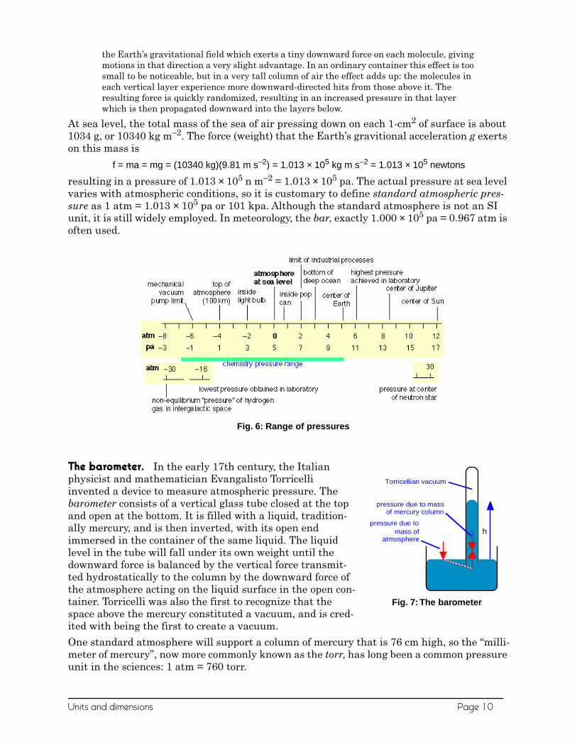
Fig. 6: Range of pressures

pressure due tomass of

atmosphere

pressure due to massof mercury column

h

Torricellian vacuum

Fig. 7: The barometer


2 • The meaning of measure: accuracy and precisionIn science, there are numbers and there are numbers. What we ordinarily think of as a num-ber we will refer to here as a pure number is just that: an expression of a precise value. The first of these you ever learned were the counting numbers, or integers; later on, you were introduced to the decimal numbers, and the rational numbers, which include numbers such as 1/3 and π (pi) that cannot be expressed as exact decimal values.

The other kind of numeric quantity that we encounter in the natural sciences is a measured value of something– the length or weight of an object, the volume of a fluid, or perhaps the reading on an instrument. Although we express these values in the form of numbers, it would be a mistake to regard them as the kind of pure numbers described above.

Confusing? Suppose our instrument has an indicator such as you see here. The pointer moves up and down so as to display the mea-sured value on this scale. What number would you write in your notebook when recording this measurement? Clearly, the value is somewhere between 130 and 140 on the scale, but the graduations enable us to be more exact and place the value beteween 134 and 135. The indicator points more closely to the latter value, and we can go one more step by estimating the value as perhaps 134.8, so this is the value you would report for this measurement. Now here’s the important thing to understand: although “134.8” is itself a num-ber, the quantity we are measuring is almost certainly not 134.8— at least, not exactly. The reason is obvious if you note that the instrument scale is such that we are barely able to distinguish between 134.7, 134.8, and 134.9. In reporting the value 134.8 we are effectively saying that the value is probably somewhere with the range 134.75 to 134.85. In other words, there is an uncertainty of ±0.05 unit in our measurement.

Uncertainty is certain! All measurements of quantities that can assume a continuous range of values (lengths, masses, volumes, etc.) consist of two parts: the reported value itself (never an exactly known number), and the uncertainty associated with the measurement.

2.1 Error in measured valuesAll measurements are subject to error which contributes to the uncertainty of the result. By “error”, we do not mean just outright mistakes, such as incorrect use of an instrument or failure to read a scale properly; although such gross errors do sometimes happen, they usu-ally yield results that are sufficiently unexpected to call attention to themselves. Our main concern is with the kinds of errors that are inherent in any act of measuring:

Random error The more sensitive the measuring instrument, the less likely it is that two successive measurements of the same sample will yield identical results. In the example we discussed above, distinguishing between the values 134.8 and 134.9 may be too difficult to do in a consistent way, so two independent observers may record different values even when viewing the same reading. Each measurement is also influenced by a myriad of minor events, such as building vibrations, electrical fluctuations, motions of the air, and friction in any moving parts of the instrument.

Systematic error Suppose that you weigh yourself on a bathroom scale, not noticing that the dial reads “1.5 kg” even before you have placed your weight on it. Similarly, you might use an old ruler with a worn-down end to measure the length of a piece of wood. In both of these examples, all subsequent measurements, either of the same object or of different ones, will be off by a constant amount. Unlike random error, which is impossible to eliminate, these systematic errors are usually quite easy to avoid or compensate for, but only by a con-

140

130

The meaning of measure: accuracy and precision

scious effort in the conduct of the observation, usually by proper zeroing and calibration of the measuring instrument. However, once systematic error has found its way into the data, it is can be very hard to detect.

2.2 More than one answer: scatter in measured values.If you wish to measure your height to the nearest centimetre or inch, or the volume of a liq-uid cooking ingredient to the nearst “cup”, you can probably do so without having to worry about random error. The error will still be present, but its magnitude will be such a small fraction of the value that it will not be detected. Thus random error is not something we worry about too much in our daily lives.

If we are making scientific observations, however, we need to be more careful, particularly if we are trying to exploit the full sensitivity of our measuring instruments in order to achieve a result that is as reliable as possible. If we are measuring a directly observable quantity such as the weight or volume of an object, then a single measurement, carefully done and reported to a precision that is consistent with that of the measuring instrument, will usually be sufficient.

More commonly, however, we are called upon to find the value of some quantity whose deter-mination depends on several other measured values, each of which is subject to its own sources of error. Consider a common laboratory experiment in which you must determine the percentage of acid in a sample of vinegar by observing the volume of sodium hydroxide solu-tion required to neutralize a given volume of the vinegar. You carry out the experiment and obtain a value. Just to be on the safe side, you repeat the procedure on another identical sample from the same bottle of vinegar. If you have actually done this in the laboratory, you will know it is highly unlikely that the second trial will yield the same result as the first. In fact, if you run a number of replicate (that is, identical in every way) determinations, you will probably obtain a scatter of results.

To understand why, consider all the individual measurements that go into each determina-tion; the volume of the vinegar sample, your judgement of the point at which the vinegar is neutralized, and the volume of solution used to reach this point. And how accurately do you know the concentration of the sodium hydroxide solution, which was made up by dissolving a measured weight of the solid in water and then adding more water until the solution reaches some measured volume. Each of these many observations is subject to random error; because such errors are random, they can occasionally cancel out, but for most trials we will not be so lucky– hence the scatter in the results.

A similar difficulty arises when we need to determine some quantity that describes a collec-tion of objects. For example, a pharmaceutical researcher will need to determine the time required for half of a standard dose of a certain drug to be eliminated by the body, or a man-ufacturer of light bulbs might want to know how many hours a certain type of light bulb will operate before it burns out. In these cases a value for any individual sample can be deter-mined easily enough, but since no two samples (patients or light bulbs) are identical, we are compelled to repeat the same measurement on multiple samples, and once again, are faced with a scattering of results.

As a final example, suppose that you employ a super-sensitive instrument for measuring dis-tance (such as a laser ranging device, for example) in order to measure the length of a room.You make one measurement, and record the results. If you then make a similar mea-surement at a different place along the same two opposite walls of the room or along a differ-ent cross-section of the coin, you will get a different result.


Here the problem is not so much with the accuracy of any single measurement, but with the incorrect assumption that the two opposite walls of the room can be perfectly parallel planes or that the cross-section of the coin can be a perfect circle. In these cases, it turns out that there is no single, true value of either quantity we are trying to measure.

2.3 Dealing with scatter: the meanWhen we obtain more than one result for a given measurement (either made repeatedly on a single sample, or more commonly, on different samples), the simplest procedure is to report the mean, or average value. The mean is defined mathematically as the sum of the values, divided by the number of measurements:

If you are not familiar with this notation, don’t let it scare you! Take a moment to see how it expresses the previous sentence; if there are n measurements, each yielding a value xi, then we sum over all i and divide by n to get the mean value xm. For example, if there are only two measurements, x1 and x2, then the mean is (x1 + x2)/2.

2.4 Accuracy and precisionWe tend to use these two terms interchangeably in our ordinary conversation, but in the con-text of scientific measurement, they have very different meanings:

• ;Accuracy refers to how closely the measured value of a quantity corresponds to its “true” value.

• ;Precision expresses the degree of reproducibility, or agreement between repeated measure-ments.

Accuracy, of course, is the goal we strive for in scientific measurements. Unfortunately, how-ever, there is no obvious way of knowing how closely we have achieved it; the “true” value, whether it be of a well-defined quantity such as the mass of a particular object, or an aver-age that pertains to a collection of objects, can never be known– and thus we can never rec-ognize it if we are fortunate enough to find it.

??

xx

nmii= ∑

10.2 10.3 10.4 10.5 10.6 10.7 0

1

2

3

num

ber

of r

esul

ts

Problem example: Calculate the mean value of the measurements illustrated on the right.Solution: There are eight data points (10.4 was found in three trials, 10.5 in two), so n = 8. The mean is

(10.2 + 10.3 + 10.4 + 10.4 + 10.4 + 10.5 + 10.5 + 10.6) / 8= 10.4..


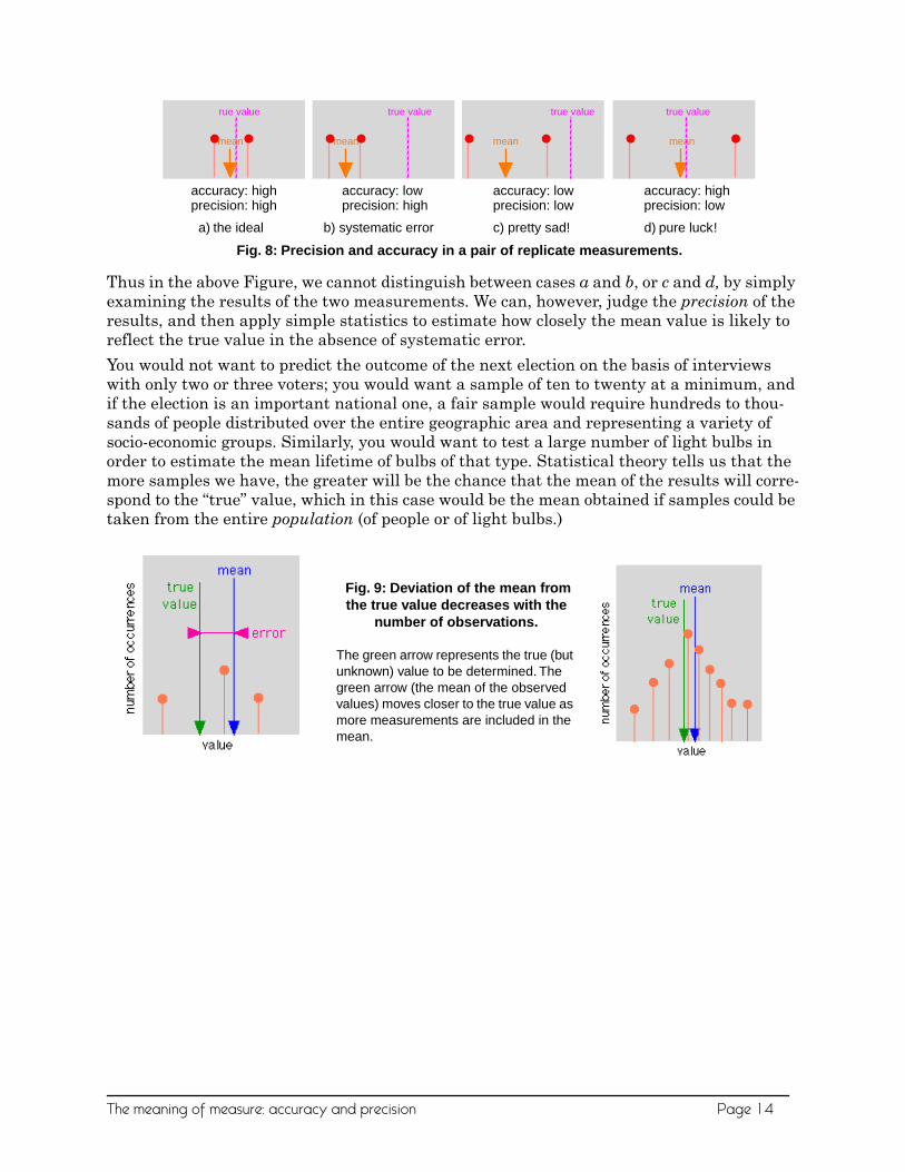
Thus in the above Figure, we cannot distinguish between cases a and b, or c and d, by simply examining the results of the two measurements. We can, however, judge the precision of the results, and then apply simple statistics to estimate how closely the mean value is likely to reflect the true value in the absence of systematic error.

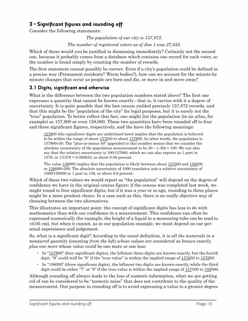
You would not want to predict the outcome of the next election on the basis of interviews with only two or three voters; you would want a sample of ten to twenty at a minimum, and if the election is an important national one, a fair sample would require hundreds to thou-sands of people distributed over the entire geographic area and representing a variety of socio-economic groups. Similarly, you would want to test a large number of light bulbs in order to estimate the mean lifetime of bulbs of that type. Statistical theory tells us that the more samples we have, the greater will be the chance that the mean of the results will corre-spond to the “true” value, which in this case would be the mean obtained if samples could be taken from the entire population (of people or of light bulbs.)

rue value

mean

true value

mean

true value

mean

true value

mean

accuracy: highprecision: high

accuracy: lowprecision: high

accuracy: lowprecision: low

accuracy: highprecision: low

a) the ideal b) systematic error c) pretty sad! d) pure luck!

Fig. 8: Precision and accuracy in a pair of replicate measurements.

Fig. 9: Deviation of the mean from the true value decreases with the

number of observations.

The green arrow represents the true (but unknown) value to be determined. The green arrow (the mean of the observed values) moves closer to the true value as more measurements are included in the mean.


2.5 Absolute and relative uncertaintyIf you weigh out 74.1 mg of a solid sample on a laboratory balance that is accurate to within 0.1 milligram, then the actual weight of the sample is likely to fall somewhere in the range of 74.0 to 74.2 mg; the absolute uncertainty in the weight you observe is 0.2 mg, or ±0.1 mg. If you use the same balance to weigh out 3.2914 g of another sample, the actual weight is between 3.2913 g and 3.2915 g, and the absolute uncertainty is still ±0.1 mg.

Although the absolute uncertainties in these two examples are identical, we would probably consider the second measurement to be more precise because the uncertainty is a smaller fraction of the measured value. The relative uncertainties of the two results would be

0.2 ÷ 74.1 = 0.0027 (about 3 parts in 1000 (PPT), or 0.3%)0.0002 ÷ 08 = 3.2913 = 0.000084 (about 0.8 PPT , or 0.008 %)

Relative uncertainties are widely used to express the reliability of measurements, even those for a single observation, in which case the uncertainty is that of the measuring device. Relative uncertainties can be expressed as parts per hundred (percent), per thousand (PPT), per million, (PPM), and so on.


3 • Significant figures and rounding offConsider the following statements:

The population of our city is 157,872.

The number of registered voters as of Jan 1 was 27,833.

Which of these would you be justified in dismissing immediately? Certainly not the second one, because it probably comes from a database which contains one record for each voter, so the number is found simply by counting the number of records.

The first statement cannot possibly be correct. Even if a city’s population could be defined in a precise way (Permanent residents? Warm bodies?), how can we account for the minute-by minute changes that occur as people are born and die, or move in and move away?

3.1 Digits, significant and otherwiseWhat is the difference between the two population numbers stated above? The first one expresses a quantity that cannot be known exactly– that is, it carries with it a degree of uncertainty. It is quite possible that the last census yielded precisely 157,872 records, and that this might be the “population of the city” for legal purposes, but it is surely not the “true” population. To better reflect this fact, one might list the population (in an atlas, for example) as 157,900 or even 158,000. These two quantities have been rounded off to four and three significant figures, respectively, and the have the following meanings:

157900 (the significant digits are underlined here) implies that the population is believed to be within the range of about 157850 to about 157950. In other words, the population is 157900±50. The “plus-or-minus 50” appended to this number means that we consider the absolute uncertainty of the population measurement to be 50 – (–50) = 100. We can also say that the relative uncertainty is 100/157900, which we can also express as 1 part in 1579, or 1/1579 = 0.000633, or about 0.06 percent.

The value 158000 implies that the population is likely between about 157500 and 158500, or 158000±500. The absolute uncertainty of 1000 translates into a relative uncertainty of 1000/158000 or 1 part in 158, or about 0.6 percent.

Which of these two values we would report as “the population” will depend on the degree of confidence we have in the original census figure; if the census was completed last week, we might round to four significant digits, but if it was a year or so ago, rounding to three places might be a more prudent choice. In a case such as this, there is no really objective way of choosing between the two alternatives.

This illustrates an important point: the concept of significant digits has less to do with mathematics than with our confidence in a measurement. This confidence can often be expressed numerically (for example, the height of a liquid in a measuring tube can be read to ±0.05 cm), but when it cannot, as in our population example, we must depend on our per-sonal expereience and judgement.

So, what is a significant digit? According to the usual definition, it is all the numerals in a measured quantity (counting from the left) whose values are considered as known exactly, plus one more whose value could be one more or one less:

• ;In “157900” (four significant digits), the leftmost three digits are known exactly, but the fourth digit, “9” could well be “8” if the “true value” is within the implied range of 157850 to 157950.

• ;In “158000” (three significant digits), the leftmost two digits are known exactly, while the third digit could be either “7” or “8” if the true value is within the implied range of 157500 to 158500.

Although rounding off always leads to the loss of numeric information, what we are getting rid of can be considered to be “numeric noise” that does not contribute to the quality of the measurement. Our purpose in rounding off is to avoid expressing a value to a greater degree

Significant figures and rounding off

of certainty than is consistent with the undertainty in the measurement.

Implied uncertainties. If you know that a balance is accurate to within 0.1 mg, say, then the uncertainty in any measurement of mass carried out on this balance will be ±0.1 mg. Suppose, however, that you are simply told that an object has a length of 0.42 cm, with no indication of its precision. In this case, all you have to go on is the number of digits contained in the data. Thus the quantity “0.42 cm” is specified to 0.01 unit in 0 42, or one part in 42 . The implied relative uncertainty in this figure is 1/42, or about 2%. The precision of any numeric answer calculated from this value is therefore limited to about the same amount.

Round-off error. It is important to understand that the number of significant digits in a value provides only a rough indication of its precision, and that information is lost when rounding off occurs.

Suppose, for example, that we measure the weight of an object as 3.28 g on a balance believed to be accurate to within ±0.05 gram. The resulting value of 3.28±.05 gram tells us that the true weight of the object could be anywhere between 3.23 g and 3.33 g. The absolute uncertainty here is 0.1 g (±0.05 g), and the relative uncertainty is 1 part in 32.8, or about 3 percent.

How many significant digits should there be in the reported measurement? Since only the leftmost “3” in “3.28” is certain, you would probably elect to round the value to 3.3 g. So far, so good. But what is someone else supposed to make of this figure when they see it in your report? The value “3.3 g” suggests an implied uncertainty of 3.3±0.05 g, meaning that the true value is likely between 3.25 g and 3.35 g. This range is 0.02 g below that associated with the orginal measurement, and so rounding off has intro-duced a bias of this amount into the result. Since this is less than half of the ±0.05 g uncer-tainty in the weighing, it is not a very serious matter in itself. However, if several values that were rounded in this way are combined in a calculation, the rounding-off errors could become noticeable.

3.2 Rules for rounding offThe standard rules for rounding off are well known. Before we set them out, let us agree on what to call the various components of a numeric value.

• ;The most significant digit is the leftmost digit (not counting any leading zeros which function only as placeholders and are never significant digits.)

• ;If you are rounding off to n significant digits, then the least significant digit is the nth digit from the most significant digit.The least significant digit can be a zero.

• ;The first non-significant digit is the n+1th digit.

The the rules themselves are:• ;If the first non-significant digit is less than 5, then the least significant digit remains

unchanged.

• ;If the first non-significant digit is greater than 5, the least significant digit is increased by 1.

• ;If the first non-significant digit is 5, the least significant digit can usually either be incre-mented or left unchanged*.

• ;All non-significant digits are removed.

*Students are sometimes told to increment the least significant digit by 1 if it is odd, and to leave it unchanged if it is even. One wonders if this reflects some superstition that even

3.363.343.323.303.283.263.243.22

range of implied uncertainty in “3.3” g.

range ofuncertainty in

originalmeasurement


numbers are somehow “better” than odd ones! In fact, you could just as well do it the other way around, incrementing only the even numbers. If you are only rounding a single num-ber, it doesn’t really matter what you do. However, when you are rounding a series of num-bers that will be used in a calculation, if you treated each first-nonsignificant 5 in the same way, you would be over- or underestating the value of the rounded number, thus accumu-lating round-off error. Since there are equal numbers of even and odd digits, incrementing only the one kind will keep this kind of error from building up. You could do just as well, of course, by flipping a coin!

The following table illustrates these rules.

Rounding up the nines. Suppose that an object is found to have a weight of 3.98 ± 0.05 g. This would place its true weight somewhere in the range of 3.93 g to 4.03 g. In judging how to round this number, you count the number of digits in “3.98” that are known exactly, and you find none! Since the “4” is the leftmost digit whose value is uncertain, this would imply that the result should be rounded to one significant figure and reported simply as 4 g. An alternative would be to bend the rule and round off to two significant digits, yielding 4.0 g. How can you decide what to do?

In a case such as this, you should look at the implied uncertainties in the two values, and compare them with the uncertainty associated with the original measurement.

Rounding off to two digits is clearly the only reasonable course.

The same kind of thing could happen if the original measurement was 9.98 ± 0.05 g. Again, the true value is believed to be in the range of 10.03 g to 9.93 g. The fact that no digit is certain here is an artifact of decimal notation. The absolute uncertainty in the observed value is 0.1 g, so the value itself is known to about 1 part in 100, or 1%. Rounding this value to three digits yields 10.0 g with an implied uncertainty of ±.05 g, or 1 part in 100, consistent with the uncertainty in the observed value.

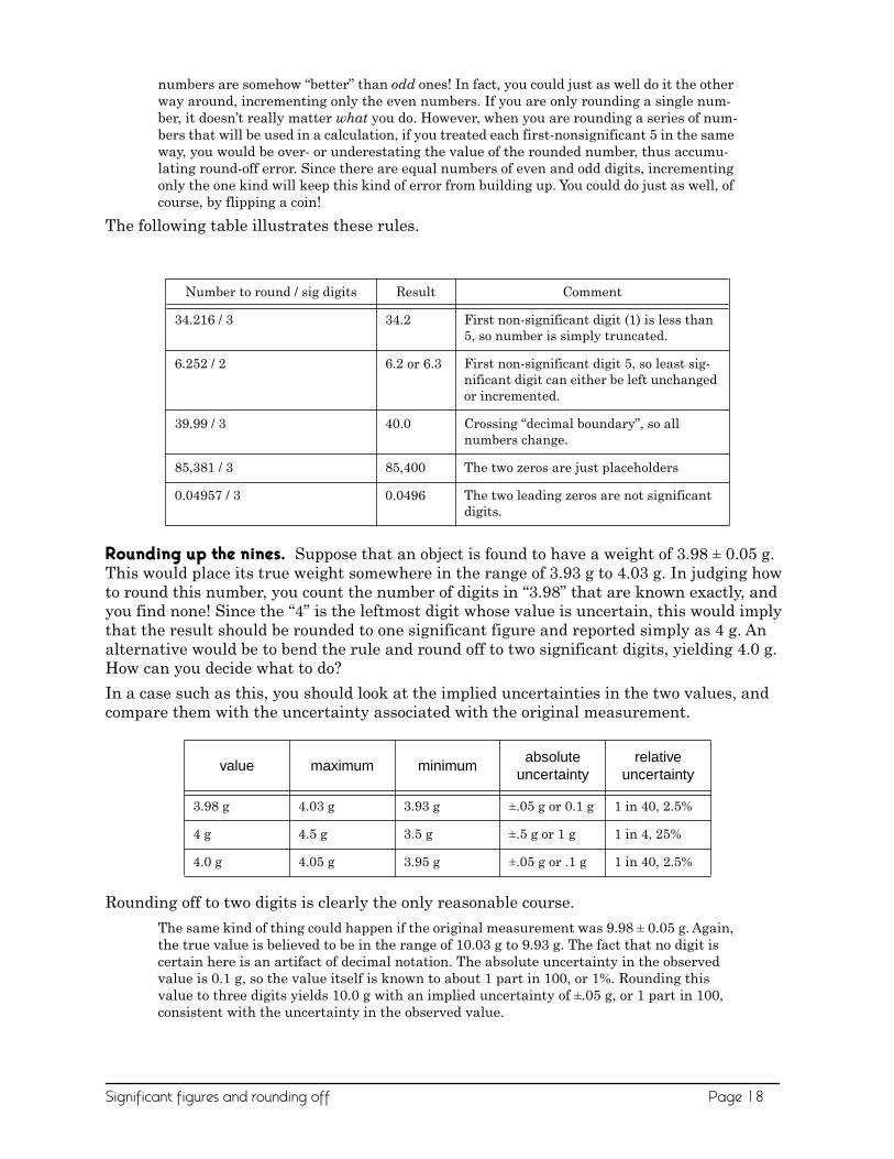
Number to round / sig digits Result Comment

34.216 / 3 34.2 First non-significant digit (1) is less than 5, so number is simply truncated.

6.252 / 2 6.2 or 6.3 First non-significant digit 5, so least sig-nificant digit can either be left unchanged or incremented.

39.99 / 3 40.0 Crossing “decimal boundary”, so allnumbers change.

85,381 / 3 85,400 The two zeros are just placeholders

0.04957 / 3 0.0496 The two leading zeros are not significant digits.

value maximum minimumabsolute

uncertaintyrelative

uncertainty

3.98 g 4.03 g 3.93 g ±.05 g or 0.1 g 1 in 40, 2.5%

4 g 4.5 g 3.5 g ±.5 g or 1 g 1 in 4, 25%

4.0 g 4.05 g 3.95 g ±.05 g or .1 g 1 in 40, 2.5%


3.3 Rounding off the results of calculationsIn science, we frequently need to carry out calculations on measured values. For example, you might use your pocket calculator to work out the area of a rectangle:

Your calculator is of course correct as far as the pure numbers go, but you would be wrong to write down “1.57676 cm2” as the answer. Two possible options for rounding off the calculator answer are shown below:

It is clear that neither option is entirely satisfactory; rounding to 3 significant digits leaves the answer too precisely specified, whereas following the rule and rounding to 2 digits has the effect of throwing away some precision. In this case, it could be argued that rounding to three digits is justified because the implied relative uncertainty in the answer, 0.6%, is more consistent with those of the two factors.

The above example is intended to point out that the rounding-off rules, although convenient to apply, do not always yield the most desirable result.

Other examples of rounding calculated values based on measurements are given below.

rounded value precision

1.58 1 part in 158, or 0.6 %

1.6 1 part in 16, or 6 %

Observed values should be rounded off to the number of digitsthat most accurately conveys the uncertainty in the original value.

• ;Usually, this means rounding off to the number of significant digits in the quantity: the number of digits (counting from the left) that are known exactly, plus one more.

• ;When this cannot be applied (as in the cases described above when addition or subtrac-tion of the absolute uncertainty bridges a power of ten), then we round in such a way that the relative implied uncertainty in the result is as close as possible to that of the observed value.

1.57676

calculator result

.753 x 0.42 implied relative uncertainties: 0.03 % 2 %


The last of the examples shown above represents the very common operation of converting

one unit into another. There is a certain amount of ambiguity here; if we take "9 in" to mean a distance in the range 8.5 to 9.5 in, then the uncertainty is ±0.5 in, which is 1 part in 18, or about ± 6%. The relative uncertainty in the answer must be the same, since all the values are multiplied by the same factor, 2.54 cm/in. In this case we are justified in writing the answer to two significant digits, yielding an uncertainty of about ±4; if we had used the answer "20 cm" (one significant digit), its implied uncertainty would be ±5 cm, or ±25%.

calculator result rounded remarks

18.4 The numerator is specified to 1 part in 21000, but the denominator is known to 1 part in only 114 (0.9%); the rounded answer has a precision of 1 part in 184 or 0.5%.

1.9E6 The "3.1" factor is specified to 1 part in 31, or 3%. In the answer 1.9, the value is expressed to 1 part in 19, or 5%. These precisions are comparable, so the rounding-off rule has given us a reasonable result.

A certain book has a thickness of 117 mm; find the height of a stack of 24 identical books:

2810 mm The “24” and the “1” are exact, so the only uncertain value is the thickness of each book, given to 3 significant dig-its. The trailing zero in the answer is only a placeholder.

10.4 In addition or subtraction, look for the term having the smallest number of decimal places, and round off the answer to the same number of places.

Convert “9 inches” to centimeters: 23 cm [See below]

18.4412280721.0231.14

==== 1111....999933330000888877771111 EEEE66665.030 – 10—ª) – (1.19 – 10§)

3.1 – 10—ª

10.4107

.01

.0007

.4

10

9

8

inchescentimeters

22.86 cm

24.13 cm

21.59 cm

25

24

23

22

21

Rounded value = 23 cm

(2 significant digits)


4 • Assessing the reliability of measurements: simple statisticsIn this day of pervasive media, we are continually being bombarded with data of all kinds— public opinion polls, advertising hype, government reports and statements by politicians. Very frequently, the purveyors of this information are hoping to “sell” us on a product, an idea, or a way of thinking about someone or something, and in doing so, they are all too often willing to take advantage of the average person’s inability to make informed judgements about the reliability of the data, especially when it is presented in a particular context (pop-ularly known as “spin”.)

In Science, we do not have this option: we collect data and make measurements in order to get closer to whatever “truth” we are seeking, and it is essential that we provide others with a quantative assessment of their reliability.

4.1 Attributes of a measurementThe kinds of measurements we will deal with here are those in which a number of separate observations are made on individual samples taken from a larger population.

Population, when used in a statistical context, does not necessarily refer to people, but rather to the entire universe of similar samples that might exist.

For example, you might wish to determine the amount of nicotine in a manufacturering run of one million cigarettes. Because no two cigarettes are likely to be exactly identical, and even if they were, random error would cause each analysis to yield a different result, the best you can do would be to test a representative sample of, say, twenty to one hundred ciga-rettes. You take the average (mean) of these values, and are then faced with the need to esti-mate how closely this sample mean is likely to approximate the population mean. The latter is the “true value” we can never know; what we can do, however, is make a reasonable esti-mate of the likelyhood that the sample mean does not differ from the population mean by more than a certain amount.

The attributes we can assign to an individual set of measurements of some quantity x are• ;the number of samples, n.

• ;the mean value of x (commonly known as the average), defined as

• ;the median value, which we will not deal with in this brief presentation, but is essentially the one in the middle of the list resulting from writing the individual values in order of increasing or decreasing magnitude.

• ;the range, which is the difference between the largest and smallest value in the set.

Problem example: Find the median value and range of the set of measurements depicted here.Solution: This set contains 8 measurements. The range is (10.7 – 10.3) = 0.4, and the mean value is

0.2 10.3 10.4 10.5 10.6 10.7 num

ber

of o

ccur

ance

s

10.3 + 10.4 + (3 × 10.5) + (2 × 10.6) + 10.78

= 10.5x =

Assessing the reliability of measurements: simple statistics

4.2 Dispersion of the meanSuppose that instead of taking the eight measure-ments as in the above example, we had made only two observations which, by chance, yielded the val-ues that are highlighted here. This would result in a sample mean of 10.45. Of course, any number of other pairs of values could equally well have been observed, including multiple occurances of any sin-gle value, such as 10.6.

Shown at the right are the results of two possible pairs of observations, each giving rise to its own sample mean. Assuming that all observations are subject only to random error, it is easy to see that successive pairs of experiments could yield many other sample means. The range of possible sample means is known as the dispersion of the mean.

It is clear that both of the two sample means cannot correspond to the population mean, whose value we are really trying to discover. In fact, it is quite likely that neither sample mean is the “correct” one in this sense. It is a fundamental principle of statistics, however, that the more observations we make in order to obtain a sample mean, the smaller will be the dispersion of the sample means that result from repeated sets of the same number of observations. (This is important; please read the preceding sentence at least three times to make sure you understand it!)

What is stated above is just another way of saying what you probably already know: larger samples produce more reliable results. This is the same principle that tells us that flipping a coin 100 times will be more likely to yield a 50:50 ratio of heads to tails than will be found if only ten flips (observations) are made.

0.2 10.3 10.4 10.5 10.6 10.7 num

ber

of o

ccur

ance

s

0.2 10.3 10.4 10.5 10.6 10.7 num

ber

of o

ccur

ance

s dispersion of the mean

meantrue

value

meantrue

value

error

many measurements fewer measurements

Fig. 10: How the dispersion of the mean depends on the number

of observations.The difference between the sample mean and the population mean (here indicated as the true value) is the error of the measurement. It is clear that this error diminishes as the num-ber of observations is made larger.


The reason for this inverse relation between the sample size and the dispersion of the mean is that if the factors giving rise to the different observed val-ues are truly random, then the more samples we observe, the more likely will these errors cancel out. It turns out that if the errors are truly random, then as you plot the number of occurences of each value, the results begin to trace out a very special kind of curve.

The significance of this is much greater than you might at first think, because the gauss-ian curve has special mathematical properties that we can exploit, through the methods of statistics, to obtain some very useful information about the reliability of our data.

4.3 Systematic errorThe scatter in measured results that we have been discussing arises from random variations in the myriad of events that affect the observed value, and over which the experimenter has no or only limited control. If we are trying to determine the properties of a collection of objects (nicotine content of cigarettes or lifetimes of lamp bulbs), then random variations between individual members of the population are an additional contributing factor. This type of error is called random or indeterminate error, and it is the only kind we can deal with directly by means of statistics.

There is, however, another type of error that can afflict the mea-suring process. It is known as systematic or determinate error, and its effect is to shift an entire set of data points by a constant amount. Systematic error, unlike random error, is not apparent in the data itself, and must be explicitly looked for in the design of the experiment.

One common source of systematic error is failure to use a reli-able measuring scale, or to not view a scale properly. For exam-ple, you might be measuring the length of an object with a ruler whose left end is worn, or misreading the volume of liquid in a burette by looking at the top of the meniscus rather than at its bottom, or not having your eye level with the object being viewed against the scale, thus introducing parallax error.

number of occurrences

observed values

10 20 30 40 50 60

meantrue value

error

1 2

1 212.3

12.4

12.5

12.6

parallax error

Fig. 11: Some common sources of systematic error


Blanks. Many kinds of measurements are made by devices that produce a response of some kind (often an electric current) that is directly proportional to the quan-tity being measured.For example, you might determine the amount of dissolved iron in a solution by adding a reagent that reacts with the iron to give a red color, which you measure by observing the intensity of green light that passes through a fixed thickness of the solution. In a case such as this, it is common practice to make two additional measurements.

• ;One measurement is done on a solution as similar to the unknowns as possible except that it contains no iron at all. This sample is called the blank. You adjust a control on the photometer to set its reading to zero when examining the blank.

• ;The other measurement is made on a sample containing a known concentration of iron; this is usually called the control. You adjust the sensitivity of the photometer to produce a reading of some arbitrary value (100, say) with the control solution. Assuming the photometer reading is directly proportional to the concentration of iron in the sample (this might also have to be checked, in which case a calibration curve must be consructed), the photometer reading can then be converted into iron concentration by simple proportion.

4.4 Putting statistics to work: assessing reliabilityConsider the two pairs of observations depicted here:

Notice that the sample means happen to have the same value of “40” (pure luck!), but the difference in the precisions of the two measurements makes it obvious that the set shown on the right is more reliable. How can we express this fact in a succinct way? We might say that one experiment yields a value of 40 ±20, and the other 40 ±5. Although this information might be useful for some purposes, it is unable to provide an answer to such questions as "how likely would another independent set of measurements yield a mean value within a certain range of values?" The answer to this question is perhaps the most meaningful way of assessing the "quality" or reliability of experimental data, but obtaining such an answer requires that we employ some formal statistics.

1. ;We begin by looking at the differences between the sample mean and the individual data val-ues used to compute the mean. These differences are known as deviations from the mean,xi – xmean. These values are depicted below; note that the only difference from the plots above is the mean value occurs at 0 on the horizonal axis.

2. Next, we need to find the average of these deviations. Taking a simple average, however, will not distinguish between these two particular sets of data, because both deviations average out to zero. We therefore take the average of the squares of the deviations (squaring makes the signs of the deviations disappear so they cannot cancel out). Also, we compute the average by

10 20 30 40 50 60

"blank"(true value = 0)

"control"(true value = 50)

10 20 30 40 50 60 70 10 20 30 40 50 60 70

-30 -20 -10 0 +10 +20 +30 -30 -20 -10 0 +10 +20 +30

deviations from the

mean


dividing by one less than the number of measurements, that is, by n–1 rather than by n.1The result, usually denoted by S2, is known as the variance:

3. Finally, we take the square root of the variance to obtain the standard deviation S:

This is the most important formula in statistics; it is so widely used that most scientific cal-culators provide built-in means of calculating S from the raw data.

Notice how the contrasting values of S reflect the difference in the precisions of the two data sets— something that is entirely lost if only the two means are considered.

4.5 The bell-shaped curveThe data sets we have been comparing each consisted of only two observations of the vari-able x; this made it easier to illustrate how S is calculated, but two data points is far too few for a proper statistical analysis. Suppose, for purposes of illustration, that we had accumu-lated many more data points but the standard deviations of the two sets remain as before.

Although we cannot ordinarily know the value of the population mean µ, we can assign to each data point a quantity (x – µ) which we call the deviation from the [population] mean, an index of how far each data point differs from the “true value”. We now divide this deviation from the mean by the standard deviation of the entire data set:

If we plot the values of z that correspond to each data point, we obtain the following curves for the two data sets we are using as examples:

1. The reason for dividing by n–1 is too involved to get into here. Notice, however, that the distinction beteween n and 1–n diminishes as the number of observations becomes large.

S2 xi xm–( )2∑

n 1–------------------------------=

Sxi xm–( )2∑n 1–

------------------------------=

Problem Example:

Calculate the variance and standard deviation for each of the two data sets shown on the previous page.

Solution: Substitution into the two formulas yields the results shown above.

data values 20, 60 35, 45

sample mean 40 40

variance S2

standard deviation S

28 7.1

(-20)2 + (20)2

2 – 1= 800

(–5)2 + (5)2

2 – 1= 50

z x µ–S

------------=


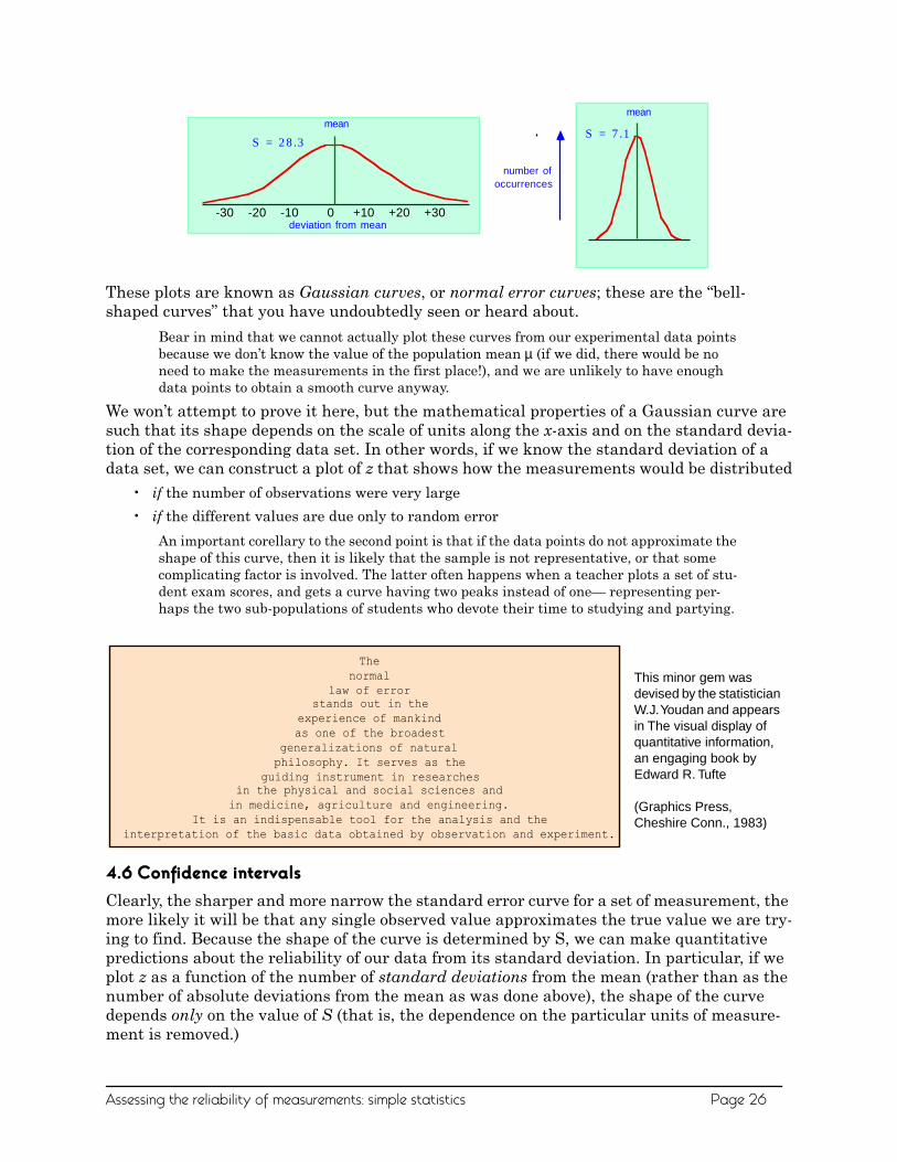
These plots are known as Gaussian curves, or normal error curves; these are the “bell-shaped curves” that you have undoubtedly seen or heard about.

Bear in mind that we cannot actually plot these curves from our experimental data points because we don’t know the value of the population mean µ (if we did, there would be no need to make the measurements in the first place!), and we are unlikely to have enough data points to obtain a smooth curve anyway.

We won’t attempt to prove it here, but the mathematical properties of a Gaussian curve are such that its shape depends on the scale of units along the x-axis and on the standard devia-tion of the corresponding data set. In other words, if we know the standard deviation of a data set, we can construct a plot of z that shows how the measurements would be distributed

• ;if the number of observations were very large

• ;if the different values are due only to random error

An important corellary to the second point is that if the data points do not approximate the shape of this curve, then it is likely that the sample is not representative, or that some complicating factor is involved. The latter often happens when a teacher plots a set of stu-dent exam scores, and gets a curve having two peaks instead of one— representing per-haps the two sub-populations of students who devote their time to studying and partying.

4.6 Confidence intervalsClearly, the sharper and more narrow the standard error curve for a set of measurement, the more likely it will be that any single observed value approximates the true value we are try-ing to find. Because the shape of the curve is determined by S, we can make quantitative predictions about the reliability of our data from its standard deviation. In particular, if we plot z as a function of the number of standard deviations from the mean (rather than as the number of absolute deviations from the mean as was done above), the shape of the curve depends only on the value of S (that is, the dependence on the particular units of measure-ment is removed.)

number of occurrences

mean

-30 -20 -10 0 +10 +20 +30 deviation from mean

S = 28.3

mean

S = 7.1

Thenormal

law of errorstands out in the

experience of mankindas one of the broadest

generalizations of naturalphilosophy. It serves as the

guiding instrument in researchesin the physical and social sciences and

in medicine, agriculture and engineering.It is an indispensable tool for the analysis and the

interpretation of the basic data obtained by observation and experiment.

This minor gem was devised by the statistician W.J. Youdan and appears in The visual display of quantitative information, an engaging book by Edward R. Tufte

(Graphics Press, Cheshire Conn., 1983)


Moreover, it can be shown that if all measurement error is truly random, 68.3 percent (about two-thirds) of the data points will fall within one standard deviation of the population mean, while 95.4 percent of the observations will differ from the population mean by no more than two standard deviations. This is extremely important, because it allows us to express the reliability of a measurement quantitatively, in terms of confidence intervals.

You might occasionaly see or hear a news report stating that the results of a certain public opinion poll are considered reliable to within, say, 5%, “nineteen times out of twenty”. This is just another way of saying that the confidence interval in the poll is 95%, the standard deviation is about 2.5% of the stated result, and that there is no more than a 5% chance that an identical poll carried out on another set of randomly-selected individuals from the same population would yield a different result.

This is as close to “the truth” as we can get in scientific measurements.

4.7 Small data sets. The more measurements we make, the more likely will their average value approximate the true value. The width of the confidence interval (expressed in the actual units of measure-ment) is directly proportional to the standard deviation and to the value of z (defined on the preceding page). The confidence interval of a single measurement in terms these quantities and of the observed sample mean is given by:

If n replicate measurements are made, the confidence interval becomes smaller:

This relation is often used “in reverse”, that is, to determine how many replicate measure-ments must be carried out in order to obtain a value within a desired confidence interval.

As we pointed out on , any relation involving the quantity z (which the standard error curve is a plot of) is of limited use unless we have some idea of the value of the population mean µ. If we make a very large number of measurements (100 to 1000, for example), then we can expect that our observed sample mean approximates µ quite closely, so there is no difficulty.

3S –2S –S 0 +S +2S +3S

68.3% confidence

interval

µ

–3S –2S –S 0 +S +2S +3S

95.4% confidence

interval

µ

10 20 30 40 50 60 70

mean

confidence interval at X-% confidence level

ppm Pb in water Fig. 12: Confidence interval and confidence level.

Take care not to confuse these two similar terms! A given CI (denoted by the shaded range of 18 - 35 ppm in the diagram) is always defined in relation to some particular CL; specifying the first without the second is meaningless. If the CI illustrated here is at the 90% CL, then a CI for a higher CL would be wider, while that for a smaller CL would cover a smaller range of values.

CI xm zS+=

CI xmzS

n-------+=


This relation is illustrated in terms of the width of the confidence interval by the Figure below, in which the magnitude of one standard deviation is much greater for the smaller set of measurements.

This is basically a result of the fact relatively large random errors tend to be less common than smaller ones, and are therefore less likely to cancel out if only a small number of mea-surements is made.

Usually, however, it is not practical to carry out a particular measurement on a sufficiently large number of samples to obtain a reliable value of µ. Thus if you were carrying out a forensic examination of tiny chip of paint, you might have only enough sample (or enough time) to do two or three replicate analyses. There are two common ways of dealing with such a difficulty.

One way of getting around this is to use pooled data; that is, to rely on similar prior determi-nations, carried out on other comparable samples, to arrive at a standard deviation that is representative of this particular type of determination.

The other common way of dealing with small numbers of replicate measurements is to look up, in a table, a quantity t, whose value depends on the number of measurements and on the desired confidence level. For example, for a confidence level of 95%, t would be 4.3 for three samples and 2.8 for five. The magnitude of the confidence interval is then given by

CI = ±t S

This procedure is not black magic, but is based on a careful analysis of the way that the Gaussian curve becomes distorted as the number of samples diminishes. It is known as Student’s t statistic.

4.8 Using statistical tests to make decisionsOnce we have obtained enough information on a given sample to evaluate parameters such as means and standard deviations, we are often faced with the necessity of comparing that sample (or the population it represents) with another sample or with some kind of a stan-dard. The following sections paraphrase some of the typical questions that can be decided by statistical tests based on the quantities we have defined above. It is important to under-stand, however, that because we are treating the questions statistically, we can only answer them in terms of statistics— that is, to a given confidence level.

The usual approach is to begin by assuming that the answer to any of the questions given

Fig. 13: How the confidence interval depends on the size of the data set.The shaded area in each plot shows the fraction of measurements that fall within two standard deviations of the population mean. It is evident that the greater the number of measurements, the more narrowly will a given fraction of them be concentrated around the supposedly “true” value.

±2S

68.3% confidence

interval

small data set

±2S

68.3% confidence

interval

large data set


below is “no” (this is called the null hypothesis), and then use the appropriate statistical test to judge the validity of this hypothesis to the desired confidence level.

Because our purpose here is to show you what can be done rather than how to do it, the fol-lowing sections do not present formulas or example calculations, which are covered in any textbook on analytical chemistry. You should concentrate here on trying to understand why questions of this kind are of importance. For more detail, see

“Should I throw this measurement out?” That is, is it likely that something other than ordinary indeterminate error is responsible for this suspiciously different result? Anyone who collects data of almost any kind will occasionally be faced with this question. Very often, ordinary common sense will be suffi-cient, but if you need some help, two statistical tests, called the Q test and the T test, are widely employed for this purpose. We won’t describe them here, but both tests involve computing a quantity (Q or T) for a particular result by means of a simple formula, and then consulting a table to determine the likelyhood that the value being questioned is a member of the popula-tion represented by the other values in the data set.

“Does this method yield reliable results? This must always be asked when trying a new method for the first time; it is essentially a matter of testing for determinate error. The answer can only be had by running the same procedure on a sample whose composition is known. The deviation of the mean value of the “known” xm from its true value µ is used to compute a Student's t for the desired confidence level. You then apply this value of t to the measurements on your unknown samples.

“Are these two samples identical?” You wish to compare the means xm1 and xm2 from two sets of measurements in order to assess whether their difference could be due to indeterminate error. Suppose, for example, that you are comparing the percent of chromium in a sample of paint removed from a car's fender with a sample found on the clothing of a hit-and-run victim. You run repli-cate analyses on both samples, and obtain different mean values, but the confidence intervals overlap. What are the chances that the two samples are in fact identical, and that the difference in the means is due solely to indeterminate error?

A fairly simple formula, using Student’s t, the standard deviation, and the numbers of rep-licate measurements made on both samples, provides an answer to this question, but only to a specified confidence level. If this is a forensic investigation that you will be presenting in court, be prepared to have your testimony demolished by the opposing lawyer if the CL is less than 99%.

Statistics at Square OneThis online reference has good descriptions of the t-test

and of the other applications described below.http://www.bmj.com/collections/statsbk/index.shtml

num

ber

of o

ccur

ance

s

A B

0 10 20 30 40 50

percent chromium


“What is the smallest quantity I can detect?” This is just a variant of the preceding question. Estimation of the detection limit of a substance by a given method begins with a set of measurements on a blank, that is, a sample in which the substance of question is assumed to be absent, but is otherwise as similar as possible to the actual samples to be tested. We then ask if any differ-ence between the mean of the blank measurements and of the sam-ple replicates can be attributed to indeterminate error at a given confidence level.

For example, a question that arises at every world Olympics event, is what is the minimum level of a drug metabolite that can be detected in an athlete's urine? Many sensitive methods are subject to random errors that can lead to a non-zero result even in a sample known to be entirely free of what is being tested for. So how far from "zero" must the mean value of a test be in order to be certain that the drug was present in a particular sample? A similar ques-tion comes up very frequently in environmental pollution studies.

4.9 How to lie with statistics: some dangerous pitfallsHow to lie with statistics is the title of an amusing book by Darrell Huff (Norton, 1954). Some of Irving Geiss’s illustrations for this book appear below.

Throwing away “wrong” answers.

It occasionally happens that a few data values are so greatly separated from the rest that they cannot reason-ably be regarded as representative. If these “outliers” clearly fall outside the range of reasonable statistical error, they can usually be disregarded as likely due to instrumen-tal malfunctions or external interferences such as mechan-ical jolts or electrical fluctuations. Some care must be exercised when data is thrown away however; There have

been a number of well-documented cases in which investigators who had certain anticipa-tions about the outcome of their experiments were able to bring these expectations about by removing conflcting results from the data set on the grounds that these particular data “had to be wrong”.

Common errors in inferential statisticshttp://www.cs.umd.edu/~mstark/exp101/traps.html

Using a too-small data set

81024

8210

0.0078

Fig. 14: Beware of small data sets!The probability of ten successive flips of a coin yielding 8 heads is given by

... indicating that it is not very likely, but can be expected to happen about eight times in a thousand runs. But there is no law of nature that says it cannot happen on your first run, so it would clearly be foolish to cry “Eureka” and stop the experi-ment after one— or even a few tries. Or to forget about the runs that did not turn up 8 heads!


Matter and measure - Chem1

Documents

Transcript of Matter and measure - Chem1