Matrices, Graphs, and PDEs: A journey of unexpected relations · I The previous statement implies...
127
Matrices, Graphs, and PDEs: A journey of unexpected relations Mario Arioli 1 1 BMS Berlin visiting Professor [email protected] http://www3.math.tu-berlin.de/Vorlesungen/SS14/MatricesGraphsPDEs/ Thanks Oliver
Transcript of Matrices, Graphs, and PDEs: A journey of unexpected relations · I The previous statement implies...

Matrices, Graphs, and PDEs:A journey of unexpected relations
Mario Arioli1
1BMS Berlin visiting [email protected]
http://www3.math.tu-berlin.de/Vorlesungen/SS14/MatricesGraphsPDEs/Thanks Oliver

Matrices, Graphs, and PDEs: A journey of unexpected relations, BMS, Berlin 2014 Mario Arioli
Lecture on sparse directsolvers
I Sparse matrices
I Ratherford-Boeing format - indirect addressingI Basic operations on sparse structures:
I permutationI scalar product between sparse vectorsI linear combination of sparse vectors
I Fill-in problem in LU decomposition
I Block Triangular Form (BTF), Reverse Cuthill-MacKee
2 / 84

Matrices, Graphs, and PDEs: A journey of unexpected relations, BMS, Berlin 2014 Mario Arioli
Sparse matrices
What is a SPARSE MATRIX A ∈ IRn×n?
I The number of non zero entries in A (nz(A)) must be O(n)i.e. If we define δ ∈ (0, 1) the density of non zeros entriesnz(A) = δn2, we assume that
1
n< δ = O(
1
n)
I The previous statement implies that A depends on a “small”number of parameters, but the reverse is not true(Vandermonde, circulant matrices, etc....)
3 / 84

Matrices, Graphs, and PDEs: A journey of unexpected relations, BMS, Berlin 2014 Mario Arioli
Sparse matrices: examples
0 500 1000 1500 2000
0
500
1000
1500
2000
nz = 24618
STOKES PROBLEM (N=2211)
Stokes problem approximation by mixed finite element method
(n = 2211)
4 / 84

Matrices, Graphs, and PDEs: A journey of unexpected relations, BMS, Berlin 2014 Mario Arioli
Sparse matrices: examples
0 10 20 30 40 50 60
0
10
20
30
40
50
60
nz = 288
LAPLACE OPERATOR (N=64)
Laplace operator approximation by the finite difference method (n = 64)
5 / 84

Matrices, Graphs, and PDEs: A journey of unexpected relations, BMS, Berlin 2014 Mario Arioli
Sparse matrices: examples
0 100 200 300 400 500 600 700 800
0
100
200
300
400
500
600
700
800
nz = 1432
Sparse Matrix (N=800)
General non symmetric sparse matrix (n = 800)
6 / 84

Matrices, Graphs, and PDEs: A journey of unexpected relations, BMS, Berlin 2014 Mario Arioli
Sparse matrices: a more complex example
Structural mechanics problem
7 / 84

Matrices, Graphs, and PDEs: A journey of unexpected relations, BMS, Berlin 2014 Mario Arioli
Sparse matrices: a more complex example
Structural mechanics problem
8 / 84

Matrices, Graphs, and PDEs: A journey of unexpected relations, BMS, Berlin 2014 Mario Arioli
Sparse matrices: a more complex example
Mesh
9 / 84

Matrices, Graphs, and PDEs: A journey of unexpected relations, BMS, Berlin 2014 Mario Arioli
Sparse matrices: a more complex example
A with n = 42339 nz(A) = 3095034 and δ = 0.0017
10 / 84

Matrices, Graphs, and PDEs: A journey of unexpected relations, BMS, Berlin 2014 Mario Arioli
Sparse matrices: Ambiguous definition
I What is a good δ?
I If A is a vector: δ = 0.1? δ = 0.001?
I The choice will depend on n
11 / 84

Matrices, Graphs, and PDEs: A journey of unexpected relations, BMS, Berlin 2014 Mario Arioli
Sparse matrices: Ambiguous definition
I What is a good δ?
I If A is a vector: δ = 0.1? δ = 0.001?
I The choice will depend on n
11 / 84

Matrices, Graphs, and PDEs: A journey of unexpected relations, BMS, Berlin 2014 Mario Arioli
Sparse matrices: Ambiguous definition
I What is a good δ?
I If A is a vector: δ = 0.1? δ = 0.001?
I The choice will depend on n
11 / 84

Matrices, Graphs, and PDEs: A journey of unexpected relations, BMS, Berlin 2014 Mario Arioli
Sparse vectors: storage
A sparse vector may be held in a full-lenght vector storage: rapidaccess but arather wasteful of storage.
I If v is a n-vector: (vi , i) is enough. We have a real vector VALand an integer vector IND, each of lenght at least the numberof entries (NZV ≤ N. VAL(J)= vi and IND(J) = i J =
1,NZV.
I gather is the operation of transforming a full vector to packedform
I scatter is the reverse operation
12 / 84

Matrices, Graphs, and PDEs: A journey of unexpected relations, BMS, Berlin 2014 Mario Arioli
Sparse vectors: inner product of two packed vectors
Let (VALX,INDX) and (VALY,INDY) two packed vectors of lengthNZX and NZY
do K = 1,N
W(K) = 0
end do
PROD = 0
do KX = 1,NZX
W(INDX(KX)) = VALX(KX)
end do
do KY = 1,NZY
PROD = PROD + W(INDY(KY))*VAL(KY)
end do
13 / 84

Matrices, Graphs, and PDEs: A journey of unexpected relations, BMS, Berlin 2014 Mario Arioli
Sparse vectors: x = x + αy
Let (VALX,INDX) and (VALY,INDY) two packed vectors of lenghtNZX and NZY
do K = 1,NZY
W(INDX(K)) = VALY(K)
end do
do KX = 1,NZX
I = INDX(KX)
if (W(I) .NE. ZERO) then
VALX(KX) = VALX(KX) + ALPHA*W(I)
W(I) = ZERO
end if
end do
do KY = 1,NZY
I = INDX(KY)
if (W(I) .NE. ZERO) then
NZX = NZX + 1
VALX(NZX) = ALPHA*W(I)
INDX(NZX) = I
W(I) = ZERO
end if
end do
14 / 84

Matrices, Graphs, and PDEs: A journey of unexpected relations, BMS, Berlin 2014 Mario Arioli
Sparse vectors: x = x +∑
j αjy(j)
1. Load x in w
2. For each y(j) : Scan y(j). For each y(j)i , check wi . If is
nonzero, set wi = wi + αjy(j)i and add i to the data structure
for x
3. Scan the revised data structure for x. For each i , setxi = wi , wi = 0
15 / 84

Matrices, Graphs, and PDEs: A journey of unexpected relations, BMS, Berlin 2014 Mario Arioli
Sparse vectors: permutations
A permutation matrix P can be represented by a set of integers
ipos(i) i = 1, . . . , n
which represent the position of the components of x in y = Px
example: ipos = [2, 4, 3, 1, 6, 5, 8, 7]
The permuted vector can be computed as followdo I = 1,N
Y(IPOS(I)) = X(I)
end do
example: x = [x1, 0, 0, x4, 0, 0, x7, 0], y = [0, x4, 0, x1, 0, 0, 0, x7]
The inverse permutation invipos can be easily computeddo I = 1,N
INVIPOS(IPOS(I)) = I
end do
example: invipos = [4, 1, 3, 2, 6, 5, 8, 7]
16 / 84

Matrices, Graphs, and PDEs: A journey of unexpected relations, BMS, Berlin 2014 Mario Arioli
Sparse vectors: permutations
A permutation matrix P can be represented by a set of integers
ipos(i) i = 1, . . . , n
which represent the position of the components of x in y = Pxexample: ipos = [2, 4, 3, 1, 6, 5, 8, 7]The permuted vector can be computed as followdo I = 1,N
Y(IPOS(I)) = X(I)
end do
example: x = [x1, 0, 0, x4, 0, 0, x7, 0], y = [0, x4, 0, x1, 0, 0, 0, x7]The inverse permutation invipos can be easily computeddo I = 1,N
INVIPOS(IPOS(I)) = I
end do
example: invipos = [4, 1, 3, 2, 6, 5, 8, 7]
16 / 84

Matrices, Graphs, and PDEs: A journey of unexpected relations, BMS, Berlin 2014 Mario Arioli
Sparse vectors: permutations
The sparse vector x can be permuted in place by
do I = 1,NZX
INDX(I) = INVIPOS(INDX(I))
end do
example: x = [x1, 0, 0, x4, 0, 0, x7, 0], y = [0, x4, 0, x1, 0, 0, 0, x7]invipos = [4, 1, 3, 2, 6, 5, 8, 7]indx = [1, 4, 7] → indx = [4, 2, 8]
17 / 84

Matrices, Graphs, and PDEs: A journey of unexpected relations, BMS, Berlin 2014 Mario Arioli
Sparse matrices: storage
A =
1 0 0 −1 02 0 −2 0 30 −3 0 0 00 4 0 −4 05 0 −5 0 6
Coordinate scheme
Subscripts 1 2 3 4 5 6 7 8 9 10 11
IRN 1 2 2 1 5 3 4 5 2 4 5JCN 4 5 1 1 5 2 4 3 3 2 1VAL -1 3 2 1 6 -3 -4 -5 -2 4 5
18 / 84

Matrices, Graphs, and PDEs: A journey of unexpected relations, BMS, Berlin 2014 Mario Arioli
Sparse matrices: storage
A =
1 0 0 −1 02 0 −2 0 30 −3 0 0 00 4 0 −4 05 0 −5 0 6
Collection of sparse row vectors
Subscripts 1 2 3 4 5 6 7 8 9 10 11
LENROW 2 3 1 2 3IROWST 1 3 6 7 9
JCN 4 1 5 1 3 2 4 2 3 1 5VAL -1 1 3 2 -2 -3 -4 4 -5 5 6
19 / 84

Matrices, Graphs, and PDEs: A journey of unexpected relations, BMS, Berlin 2014 Mario Arioli
Sparse matrices: fill-in and reordering
A =
x x x x x x x xx xx xx xx xx xx xx x
20 / 84

Matrices, Graphs, and PDEs: A journey of unexpected relations, BMS, Berlin 2014 Mario Arioli
Sparse matrices: fill-in and reordering
L =
xx xx x xx x x xx x x x xx x x x x xx x x x x x xx x x x x x x x
U =
x x x x x x x xx x x x x x x
x x x x x xx x x x x
x x x xx x x
x xx
21 / 84

Matrices, Graphs, and PDEs: A journey of unexpected relations, BMS, Berlin 2014 Mario Arioli
Sparse matrices: fill-in and reordering
PTAP =
x xx x
x xx x
x xx x
x xx x x x x x x x
22 / 84

Matrices, Graphs, and PDEs: A journey of unexpected relations, BMS, Berlin 2014 Mario Arioli
Sparse matrices: fill-in and reordering
L =
xx
xx
xx
xx x x x x x x x
U =
x xx x
x xx x
x xx x
x xx
23 / 84

Matrices, Graphs, and PDEs: A journey of unexpected relations, BMS, Berlin 2014 Mario Arioli
Sparse matrices: Block Triangular Form (BTF)
We seek permutations P and Q such that A is in block triangulaform.
PAQ =
B11
B21 B22...
......
Bk1 . . . Bk,k−1 Bkk
If the matrix A can be permute in BTF, we call it reducible,otherwise A is irriducible. We assume that all blocks Bii areirriducibles.
24 / 84

Matrices, Graphs, and PDEs: A journey of unexpected relations, BMS, Berlin 2014 Mario Arioli
Block Triangular Form (BTF): example
0 100 200 300 400 500 600 700 800
0
100
200
300
400
500
600
700
800
nz = 1432
Sparse Matrix (N=800)
General non symmetric sparse matrix (n = 800)
25 / 84

Matrices, Graphs, and PDEs: A journey of unexpected relations, BMS, Berlin 2014 Mario Arioli
Block Triangular Form (BTF): example
0 100 200 300 400 500 600 700 800
0
100
200
300
400
500
600
700
800
nz = 1183
L−factor (n=800)
L factor (n = 800)
26 / 84

Matrices, Graphs, and PDEs: A journey of unexpected relations, BMS, Berlin 2014 Mario Arioli
Block Triangular Form (BTF): example
0 100 200 300 400 500 600 700 800
0
100
200
300
400
500
600
700
800
nz = 1193
U factor (n=800)
U factor (n = 800)
27 / 84

Matrices, Graphs, and PDEs: A journey of unexpected relations, BMS, Berlin 2014 Mario Arioli
Block Triangular Form (BTF): example
0 100 200 300 400 500 600 700 800
0
100
200
300
400
500
600
700
800
nz = 1432
Reordered by Dulmage−Mendelsohn (n=800)
After application of Dulmage-Mendelsohn algorithm in Matlab (n = 800)
In Matlab it is better to compute the upper triangular version
28 / 84

Matrices, Graphs, and PDEs: A journey of unexpected relations, BMS, Berlin 2014 Mario Arioli
Block Triangular Form (BTF)
The algorithm (see Duff, Erisman, and Reid Ch-6) is based of twoseparate phases
I Maximum Transversal by computing P: the diagonal of PA isfull.
I Symmetric permutation of PA to Lower BTF: QT (PA)QTarjan (1972), Duff and Reid (1978) , HSL MC23 FORTRANimplementation (75 instructions)
29 / 84

Matrices, Graphs, and PDEs: A journey of unexpected relations, BMS, Berlin 2014 Mario Arioli
Block Tridiagonal Form and graphs
A symmetrically structured matrix has bandwidth 2m − 1 andsemibandwidth m if m is the smallest integer such that aij = 0
whenever |i − j | > m. The fill-in is confined in the band.
0 10 20 30 40 50 60
0
10
20
30
40
50
60
nz = 288
LAPLACE OPERATOR (N=64)
Laplace operator approximation by the finite difference method (n = 64,
m = 8)
30 / 84

Matrices, Graphs, and PDEs: A journey of unexpected relations, BMS, Berlin 2014 Mario Arioli
Block Tridiagonal Form and graphs
0 10 20 30 40 50 60
0
10
20
30
40
50
60
nz = 519
Factor L in a band matrix
Laplace operator approximation by the finite difference method (n = 64,
m = 8) L factor
31 / 84

Matrices, Graphs, and PDEs: A journey of unexpected relations, BMS, Berlin 2014 Mario Arioli
Block Tridiagonal Form and graphs
We can associate to the symmetrically structured matrix a graphand any renumbering of the nodes corresponds to a symmetricpermutation of the matrix. The number of arcs incident in onenode is the degree of the node. The degree of node i correspondsto the number of nonzeros in row i of the matrix.
Laplace operator approximation by the finite difference method (n = 64,
m = 8)
32 / 84

Matrices, Graphs, and PDEs: A journey of unexpected relations, BMS, Berlin 2014 Mario Arioli
Block Tridiagonal Form and graphs
We divide the nodes in level sets Si . S1 consists of one node ofminimum degree. The general level set SI consists of all theneighbours of nodes in Si−1 that are not in Si−1 or Si−2.
Laplace operator approximation by the finite difference method (n = 64,
m = 8)
33 / 84

Matrices, Graphs, and PDEs: A journey of unexpected relations, BMS, Berlin 2014 Mario Arioli
Block Tridiagonal Form and graphs
Renumbering the nodes in the level sets, we have a tridiagonalmatrix where the diagonal block i consists of the nodes in level setSi .We can improve the number of diagonal block restarting theprocess from one of the nodes in the final level set(pseudoperipheral nodes).The resulting order is called the Cuthill-McKee order.George (1971) proved that reversing the order (ReverseCuthill-McKee order) decreases the fill-in in the Gaussfactorization.
34 / 84

Matrices, Graphs, and PDEs: A journey of unexpected relations, BMS, Berlin 2014 Mario Arioli
Ordering, Frontal, Multifrontal
I Ordering of sparse matrices: Nested Dissection, minimumdegree, and approximate minimum degree.
I Threshold pivoting and its control
I Frontal e multifrontal methods
35 / 84

Matrices, Graphs, and PDEs: A journey of unexpected relations, BMS, Berlin 2014 Mario Arioli
Cholesky via Schur complement
A =
[d1 vT1v1 H1
]=
[ √d1 0
v1/√
d1 In−1
] [1 00 S1
] [ √d1 vT1 /
√d1
0 In−1
]= L1A1LT
1
S1 = H1 −v1vT1
d1
Repeat the operation on S1. L = Ln−1 . . .L1
36 / 84

Matrices, Graphs, and PDEs: A journey of unexpected relations, BMS, Berlin 2014 Mario Arioli
Cholesky via Graph theory: notations
P(A) = {(i , j)|aij 6= 0 and i 6= j}F = L + LT
P(F) = {(i , j)|fij 6= 0 and i 6= j}
P(B) is the pattern of the matrix B. Let (N ) be the set {1, . . . , n}and GB = (N ,P(B)) the graph with nodes (N ) and undirectedarcs P(B). We denote by Adj(i) = {j |j 6= i , (i , j) ∈ P(B)}
P(A) ⊆ P(F)
Fill(A) = P(F)− P(A)
37 / 84

Matrices, Graphs, and PDEs: A journey of unexpected relations, BMS, Berlin 2014 Mario Arioli
Cholesky via Graph theory: fill-in
(S1)ij 6= 0 iff (H1)ij 6= 0 or both (v1)i 6= 0 and (v1)j 6= 0
1. Delete node node x1 and all its incident arcs
2. Add arcs to the graph so that nodes in adj(x1) are pairwiseadjacent in GS1
Lemma 1 The unordered pair (xi , xj) ∈ PF iff (xi , xj) ∈ PA or(xi , xk) ∈ PF and (xj , xk) ∈ PF for some k < min{i , j}
38 / 84

Matrices, Graphs, and PDEs: A journey of unexpected relations, BMS, Berlin 2014 Mario Arioli
Graph theory: example
∗ ∗ ∗∗ ∗ ∗ ∗∗ ∗ ∗∗ ∗∗ ∗ ∗
∗ ∗ ∗
6
1
4
2 3
5
39 / 84

Matrices, Graphs, and PDEs: A journey of unexpected relations, BMS, Berlin 2014 Mario Arioli
Graph theory: example
∗ ∗ ∗∗ ∗ ∗ ∗∗ ∗ ∗∗ ∗∗ ∗ ∗
∗ ∗ ∗
6
1
4
2 3
5
39 / 84

Matrices, Graphs, and PDEs: A journey of unexpected relations, BMS, Berlin 2014 Mario Arioli
Graph theory: example
∗ ∗ ∗∗ ∗ ∗ ∗∗ ∗ ∗∗ ∗∗ ∗ ∗
∗ ∗ ∗
6
1
4
2 3
5
39 / 84
Matrices, Graphs, and PDEs: A journey of unexpected relations, BMS, Berlin 2014 Mario Arioli
Graph theory: example
∗ ∗ ∗∗ ∗ ∗ ∗∗ ∗ ∗ ∗
∗ ∗∗ ∗ ∗
∗ ∗ ∗
6
1
4
2 3
5
39 / 84

Matrices, Graphs, and PDEs: A journey of unexpected relations, BMS, Berlin 2014 Mario Arioli
Graph theory: example
∗ ∗ ∗∗ ∗ ∗ ∗∗ ∗ ∗ ∗∗ ∗ ∗∗ ∗ ∗
∗ ∗ ∗
6
1
4
2 3
5
39 / 84

Matrices, Graphs, and PDEs: A journey of unexpected relations, BMS, Berlin 2014 Mario Arioli
Graph theory: example
∗ ∗ ∗∗ ∗ ∗ ∗∗ ∗ ∗ ∗∗ ∗ ∗∗ ∗ ∗∗ ∗ ∗ ∗
6
1
4
2 3
5
39 / 84
Matrices, Graphs, and PDEs: A journey of unexpected relations, BMS, Berlin 2014 Mario Arioli
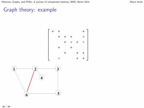
Graph theory: example
∗ ∗ ∗∗ ∗ ∗ ∗∗ ∗ ∗ ∗∗ ∗ ∗
∗ ∗ ∗∗ ∗ ∗ ∗
6
1
4
2 3
5
39 / 84

Matrices, Graphs, and PDEs: A journey of unexpected relations, BMS, Berlin 2014 Mario Arioli
Graph theory: example
∗ ∗ ∗∗ ∗ ∗ ∗∗ ∗ ∗ ∗∗ ∗ ∗∗ ∗ ∗
∗ ∗ ∗ ∗
6
1
4
2 3
5
39 / 84

Matrices, Graphs, and PDEs: A journey of unexpected relations, BMS, Berlin 2014 Mario Arioli
Graph theory: example
∗ ∗ ∗∗ ∗ ∗ ∗∗ ∗ ∗ ∗∗ ∗ ∗∗ ∗ ∗∗ ∗ ∗
6
1
4
2 3
5
39 / 84

Matrices, Graphs, and PDEs: A journey of unexpected relations, BMS, Berlin 2014 Mario Arioli
Graph theory: example
∗ ∗ ∗∗ ∗ ∗ ∗∗ ∗ ∗ ∗∗ ∗ ∗∗ ∗∗ ∗
6
1
4
2 3
5
39 / 84

Matrices, Graphs, and PDEs: A journey of unexpected relations, BMS, Berlin 2014 Mario Arioli
Graph theory: example
∗ ∗ ∗∗ ∗ ∗ ∗∗ ∗ ∗ ∗∗ ∗ ∗∗ ∗∗
6
1
4
2 3
5
39 / 84

Matrices, Graphs, and PDEs: A journey of unexpected relations, BMS, Berlin 2014 Mario Arioli
Graph theory: reachable points
6
4
2 3
5
1
Let S ⊂ N and x ∈ {N − S}. x is reachable from y through S if∃(y , v1, . . . vk , x) a path from x to y such that vi ∈ S for1 ≤ i ≤ k (k = 0⇒ any adjacent node of y not in S is reachable.
40 / 84

Matrices, Graphs, and PDEs: A journey of unexpected relations, BMS, Berlin 2014 Mario Arioli
Graph theory: reachable points
6
4
2 3
5
1
6
4
3
5
1 2
6
4
5
1 2 3
Let S ⊂ N and x ∈ {N − S}. x is reachable from y through S if∃(y , v1, . . . vk , x) a path from x to y such that vi ∈ S for1 ≤ i ≤ k (k = 0⇒ any adjacent node of y not in S is reachable.
40 / 84

Matrices, Graphs, and PDEs: A journey of unexpected relations, BMS, Berlin 2014 Mario Arioli
Graph theory: reachable sets
Definition Let S ⊂ N . The reachable set of y through S is
Reach(y , S) = {x ∈ {N − S}|x is reachable from y through S}
41 / 84

Matrices, Graphs, and PDEs: A journey of unexpected relations, BMS, Berlin 2014 Mario Arioli
Graph theory: reachable sets
Definition Let S ⊂ N . The reachable set of y through S is
Reach(y , S) = {x ∈ {N − S}|x is reachable from y through S}
������������������
������������������
������������������
������������������
������������������
������������������
������������������
������������������
ya
b c
d
Reach(y , S) = {a, b, c}
41 / 84

Matrices, Graphs, and PDEs: A journey of unexpected relations, BMS, Berlin 2014 Mario Arioli
Graph theory: reachable sets
Theorem 2
GF = {{xi , xj}|xj ∈ Reach(xi , {x1, x2, . . . , xi−1})}
Let Gi be the graph of Si the i-th Schur complement
Theorem 3Let y be a node in Gi . The set of nodes adjacent to y in Gi isgiven by
Reach(y , {x1, . . . , xi−1})
42 / 84

Matrices, Graphs, and PDEs: A journey of unexpected relations, BMS, Berlin 2014 Mario Arioli
Minimum degree algorithm
1. (Initialization) S ← ∅ . Deg(x)← |Adj(x)| ∀x ∈ N2. (Minimum degree selection ) Pick a node y ∈ {N − S} where
Deg(y) = minx∈{N−S}
Deg(x)
Number the node y next and set T ← S ∪ {y}3. (Degree update) Deg(u)← |Reach(u,T )| ∀u ∈ N − T
4. (loop or stop) If T = N stop. Otherwise set S ← T and goto 2
43 / 84

Matrices, Graphs, and PDEs: A journey of unexpected relations, BMS, Berlin 2014 Mario Arioli
Minimum degree algorithm
The implementation of the Minimum degree algorithm takesadvantage of several other results that improve the speed andreduce the complexity.It is possible to partially update the degrees using special heuristicsA good example is the APPROXIMATE MINIMUM DEGREE usedin Matlab and in HSL package MA57. The use of the AMD can beextended to matrix which are symmetric and indefinite (MA57)(See Davis, Amestoy, and Duff SIMAX, 1996 , and DuffRAL-TR-2002-024, 2002)
44 / 84

Matrices, Graphs, and PDEs: A journey of unexpected relations, BMS, Berlin 2014 Mario Arioli
Minimum degree algorithm
A with n = 42339 nz(A) = 3095034 and δ = 0.0017
45 / 84

Matrices, Graphs, and PDEs: A journey of unexpected relations, BMS, Berlin 2014 Mario Arioli
Minimun degree algorithm
after AMD
46 / 84

Matrices, Graphs, and PDEs: A journey of unexpected relations, BMS, Berlin 2014 Mario Arioli
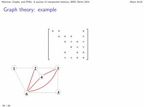
Nested Dissection
Nested Dissection Partition of the Graph of a Finite Differenceproblem matrix on a 10× 10 mesh
47 / 84
Matrices, Graphs, and PDEs: A journey of unexpected relations, BMS, Berlin 2014 Mario Arioli
Nested Dissection
Nested Dissection Permutation of a Finite Difference problemmatrix on a 10× 10 mesh
48 / 84

Matrices, Graphs, and PDEs: A journey of unexpected relations, BMS, Berlin 2014 Mario Arioli
Nested Dissection: storage requirement
The number of nonzeros in the factor L of a matrix A ∈ IRN
associated to a n × n grid (N = n2) is
31n2 log2(n)/4 +O(n2)
49 / 84

Matrices, Graphs, and PDEs: A journey of unexpected relations, BMS, Berlin 2014 Mario Arioli
Nested Dissection: complexity
The number of operations required to factor L of a matrix A ∈ IRN
associated to a n × n grid (N = n2) is
829n3/84 +O(n2 log2(n))
50 / 84

Matrices, Graphs, and PDEs: A journey of unexpected relations, BMS, Berlin 2014 Mario Arioli
Fiedler vectors
How can we generalise the process of Nested Dissection to ageneral symmetric matrix?PA − I is the adjacency matrix of a the graph supporting thematrix A. Let us denote by EA the incidence matrix of the graph.We can interpret E as a discrete divergence operator.We denote by
L = EAETA
the Graph-Laplacian .
51 / 84

Matrices, Graphs, and PDEs: A journey of unexpected relations, BMS, Berlin 2014 Mario Arioli
Fiedler vectors
L is a Laplacian with Neumann conditions!! Therefore its smallesteigenvalue is zero. Le assume that the eigenvalues λi (L) areordered in increasing order.
52 / 84

Matrices, Graphs, and PDEs: A journey of unexpected relations, BMS, Berlin 2014 Mario Arioli
Fiedler vectors
L is a Laplacian with Neumann conditions!! Therefore its smallesteigenvalue is zero. Le assume that the eigenvalues λi (L) areordered in increasing order.What about λ2(L) ?
52 / 84

Matrices, Graphs, and PDEs: A journey of unexpected relations, BMS, Berlin 2014 Mario Arioli
Fiedler vectors
.
53 / 84

Matrices, Graphs, and PDEs: A journey of unexpected relations, BMS, Berlin 2014 Mario Arioli
Fiedler vectors
Sorted eigenvector for λ2(L)
.
53 / 84

Matrices, Graphs, and PDEs: A journey of unexpected relations, BMS, Berlin 2014 Mario Arioli
Fiedler vectors
We have positive and negative values in each node. Some of themare small in absolute values! .
53 / 84

Matrices, Graphs, and PDEs: A journey of unexpected relations, BMS, Berlin 2014 Mario Arioli
Fiedler vectors
Let us separate the nodes with values ≤ −τ from the nodes withvalues ≥ τ , and from the nodes having values ∈ (−τ, τ).
53 / 84

Matrices, Graphs, and PDEs: A journey of unexpected relations, BMS, Berlin 2014 Mario Arioli
Fiedler vectors
. We can then reorder the nodes and we have
Permuted graph-Laplacian
53 / 84

Matrices, Graphs, and PDEs: A journey of unexpected relations, BMS, Berlin 2014 Mario Arioli
Fiedler vectors
In the previous example we had a separator that is√
n with n theorder of L.More generally, if such a separator does exist not only for L butalso for the the red block and the blue block then we can iteratethe process on each of them and have aGENERALISED NESTED DISSECTION (see METIS).
54 / 84

Matrices, Graphs, and PDEs: A journey of unexpected relations, BMS, Berlin 2014 Mario Arioli
Fiedler vectors
UNFORTUNATELLY it is not always the case!
55 / 84

Matrices, Graphs, and PDEs: A journey of unexpected relations, BMS, Berlin 2014 Mario Arioli
Fiedler vectors
UNFORTUNATELLY it is not always the case!
Permuted graph-Laplacian
55 / 84

Matrices, Graphs, and PDEs: A journey of unexpected relations, BMS, Berlin 2014 Mario Arioli
Fiedler vectors
UNFORTUNATELLY it is not always the case!
Sorted eigenvector for λ2(L)
55 / 84

Matrices, Graphs, and PDEs: A journey of unexpected relations, BMS, Berlin 2014 Mario Arioli
The unsymmetric matrices: Markowitz criterion
Analogously to the minimum degree criterion, we look at the Schurcomplement.
A =
[d1 wT
1
v1 H1
]=
[1 0
v1/d1 In−1
] [d1 wT
1
0 S1
]S1 = H1 −
v1wT1
d1
Repeat the operation on S1. L = Ln−1 . . .L1 and A = LU
56 / 84
Matrices, Graphs, and PDEs: A journey of unexpected relations, BMS, Berlin 2014 Mario Arioli
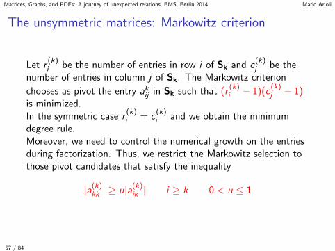
The unsymmetric matrices: Markowitz criterion
Let r(k)i be the number of entries in row i of Sk and c
(k)j be the
number of entries in column j of Sk. The Markowitz criterion
chooses as pivot the entry akij in Sk such that (r(k)i − 1)(c
(k)j − 1)
is minimized.In the symmetric case r
(k)i = c
(k)i and we obtain the minimum
degree rule.Moreover, we need to control the numerical growth on the entriesduring factorization. Thus, we restrict the Markowitz selection tothose pivot candidates that satisfy the inequality
|a(k)kk | ≥ u|a(k)ik | i ≥ k 0 < u ≤ 1
57 / 84

Matrices, Graphs, and PDEs: A journey of unexpected relations, BMS, Berlin 2014 Mario Arioli
Analysis phase and Factorization Phase
The reordering algorithms presented are heuristics:to find the permutation that minimizes the fill-in for a symmetricmatrix is a NP-complete problemFirst, we ANALYSE the data structure:
I Reordering
I Estimate if the LU factorization feasible (memoryrequirement)
I Elimination tree
Then, we can FACTORIZE
58 / 84

Matrices, Graphs, and PDEs: A journey of unexpected relations, BMS, Berlin 2014 Mario Arioli
Frontal Methods
A =m∑l=l
A[l ]
where A[l ] has nonzeros only in few rows and columns(corresponding to an element in the mesh if we are in afinite-element framework)Assembling
aij ← aij + a[l ]ij
Factorization
aij ← aij − aip(app)−1apj
can be performed as soon all the terms are assembled
59 / 84

Matrices, Graphs, and PDEs: A journey of unexpected relations, BMS, Berlin 2014 Mario Arioli
Frontal Methods
We can work only on a small matrix F , the Frontal Matrix, that isdense but with smaller dimensions compared to A
F =
[B CD E
]B is square of order k and E is square of order r : F ∈ IR(k+r)×(k+r)
k << r , typically k = 10, 20 and r = 200, ..., 500
60 / 84

Matrices, Graphs, and PDEs: A journey of unexpected relations, BMS, Berlin 2014 Mario Arioli
Frontal Methods
Front as a window
61 / 84
Matrices, Graphs, and PDEs: A journey of unexpected relations, BMS, Berlin 2014 Mario Arioli
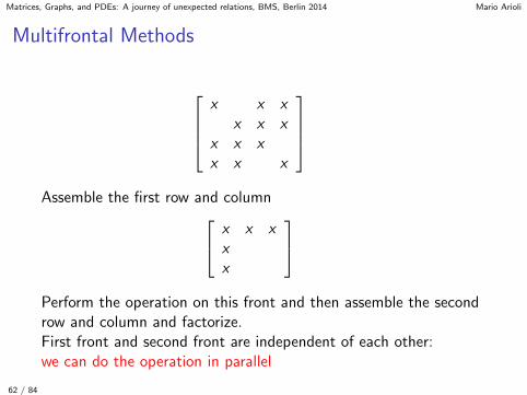
Multifrontal Methods
x x x
x x xx x xx x x
Assemble the first row and column x x x
xx
Perform the operation on this front and then assemble the secondrow and column and factorize.First front and second front are independent of each other:we can do the operation in parallel
62 / 84

Matrices, Graphs, and PDEs: A journey of unexpected relations, BMS, Berlin 2014 Mario Arioli
Multifrontal Method: elimination tree
x x x
x x xx x xx x x
4
3
1 2
Elimination tree
63 / 84

Matrices, Graphs, and PDEs: A journey of unexpected relations, BMS, Berlin 2014 Mario Arioli
Numerical pivot
I Numerical Pivot in sparse solvers
I Scaling
I A-Posteriori sparse backward error analysis
I Condition number estimators
I Iterative refinement
64 / 84

Matrices, Graphs, and PDEs: A journey of unexpected relations, BMS, Berlin 2014 Mario Arioli
Gaussian elimination
Theorem Let assume that Ais an n × n matrix of floating pointnumbers. If no zero pivots are found during the Gauss process,then the computed matrices L and U satisfy
LU = A + E
|E| ≤ 3(n − 1)ε(|A|+ |L||U|) +O(ε2)
We would like that|A| ≈ |L||U|
65 / 84

Matrices, Graphs, and PDEs: A journey of unexpected relations, BMS, Berlin 2014 Mario Arioli
Numerical Pivot in sparse solvers
We know that the partial pivot is not optimal and we haveexamples where the |L||U| is much larger than |A|
A =
1 1−1 1 1
......
......
−1 . . . −1 1
in the U factor the last column has entries that grow as2i , i = 1, . . . , n − 1
66 / 84

Matrices, Graphs, and PDEs: A journey of unexpected relations, BMS, Berlin 2014 Mario Arioli
Frontal Methods
In the Frontal Matrix, that is dense but with smaller dimensionscompared to A, we can choose the pivot only in fully assembled B.
F =
[B CD E
]If we detect a larger entry in D ( or in C), we have only twooptions:
I to delay the pivot moving the corresponding row and columnto E with the hope that further assembling operations willcure the problem. In the worst case, we will be able to takecare of this pivot in the last matrix
I to correct the value of the pivot adding to it a constant valueβ:
I β =√ε||A||
I β = ||A||
67 / 84

Matrices, Graphs, and PDEs: A journey of unexpected relations, BMS, Berlin 2014 Mario Arioli
Frontal Methods
In both cases, we need to recover the solution of Au = b.The previous corrections can be seen as perturbations of thematrix A reordered to reduce fill-in. The computed factor are thecomputed factors of
A +k∑
i=1
βieieTi
The first technique allows more pivot corrections than the secondone. If A has a condition number smaller than 1/
√ε, we can use
an iterative method to recover the solutionIn the second case, we can use the Sherman-Morrison formula tocorrect the computed solution of the perturbed problem andrecover u
68 / 84
Matrices, Graphs, and PDEs: A journey of unexpected relations, BMS, Berlin 2014 Mario Arioli
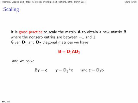
Scaling
It is good practice to scale the matrix A to obtain a new matrix Bwhere the nonzero entries are between −1 and 1.Given D1 and D2 diagonal matrices we have
B = D1AD2
and we solve
By = c y = D−12 x and c = D1b
69 / 84

Matrices, Graphs, and PDEs: A journey of unexpected relations, BMS, Berlin 2014 Mario Arioli
Scaling
There are several approach
I equilibration of the data (Curtis and Reid)
I (D1)ii = 1/||Ai•||1 or/and (D2)ii = 1/||A•i ||1I (D1)ii = 1/||Ai•||∞ or/and (D2)ii = 1/||A•i ||∞I Compute D1 and D2 such that |B| is doubly stochastic (Ruiz
2002)
All these technique improve the quality of the LU factorization anddecrease the need of choosing numerical pivots different from theones optimal for controlling the fill-in
70 / 84

Matrices, Graphs, and PDEs: A journey of unexpected relations, BMS, Berlin 2014 Mario Arioli
Rigal-Gaches (1967) theorem
∃∆A,∃δb such that:(A + ∆A)u = (b + δb)
and ‖∆A‖~k,~p ≤ S ∈ IRk×p, ‖δb‖~k ≤ t ∈ IRk
⇔‖r‖~k ≤ S‖u‖~p + twhere r is defined byr = Au− b
71 / 84

Matrices, Graphs, and PDEs: A journey of unexpected relations, BMS, Berlin 2014 Mario Arioli
Rigal-Gaches (1967) theorem: component-wise version
If we use | • | as Hypernorm, we have a component-wise version
∃∆A,∃δb such that:(A + ∆A)u = (b + δb) and|∆A| ≤ ω|A| ∈ IRn×n, |δb| ≤ ω|b| ∈ IRn
⇔|r| ≤ ω{|A||u|+ |b|}where r is defined byr = Au− b
The smallest ω satisfying the theorem (assuming 0/0 = 0) is
ω = mini
(|Au− b|)i(|A||u|+ |b|)i
‖u− u‖∞‖u‖∞
≤ ω‖|A−1|(|A||u|+ |b|)‖∞
‖u‖∞
72 / 84

Matrices, Graphs, and PDEs: A journey of unexpected relations, BMS, Berlin 2014 Mario Arioli
Condition number estimatorsThe
cond(A,u) =‖|A−1|(|A||u|+ |b|)‖∞
‖u‖∞is the Condition Number ( also known as the Bauer-Skeelcondition number) of the Problem
Au = b
Obviously, the computation of |A−1| is totally unfeasible for largesparse matrices. The pattern of the inverse will be structurally full.We would like to approximate the value in O(n2) operation.The expression ‖|A−1|d‖∞ with d ≥ 0 can be rewritten usingD = diag(d) and e = [1, 1, . . . , 1]T as follows
‖|A−1|d‖∞ = ‖|A−1|De‖∞ = ‖|A−1D|e‖∞ = ‖A−1D‖∞Then, we need a good estimator for the ‖B‖∞ or, equivalently, forthe ‖B‖1 ( B given n × n matrix).
‖B‖∞ = ‖BT‖173 / 84

Matrices, Graphs, and PDEs: A journey of unexpected relations, BMS, Berlin 2014 Mario Arioli
Condition number estimators: Hager’s algorithm
In LAPACK and in MC75 (HSL 2002) we have goodimplementation of Hager’s algorithm (SISSC 1984) for theestimate of the 1-norm of a matrix A when we are only able tocompute the matrix-vector product Av.
74 / 84

Matrices, Graphs, and PDEs: A journey of unexpected relations, BMS, Berlin 2014 Mario Arioli
Condition number estimators: Hager’s algorithm
Algorithm Given A ∈ IRn×n the algorithm computes γ and v = Aws.t. γ ≤ ‖A‖1 with ‖v‖1/‖w‖1 = γ
v = A(n−1e)if n = 1, quit with γ = |v1|, endγ = ||v||1, ξ = sign(v), x = AT ξ, k = 2repeat
j = min{i : |xvi | = ||x||∞}v = Aej , γ = γ, γ = ||v||1if sign(v) = ξ or γ ≤ γ, goto (*), endξ = sign(v), x = AT ξ, k = k + 1
until (||x||∞ = xj or k > 5
(*) xi = (−1)i+1(
1 + i−1n−1
)i = 1, . . . , n
x = Axif 2||x||1/(3n) > γ then
v = x, γ = 2||x||1/(3n)end if
75 / 84

Matrices, Graphs, and PDEs: A journey of unexpected relations, BMS, Berlin 2014 Mario Arioli
Condition number estimators
The algorithm is very reliable in practice. It is very rare for theestimate to be more than three time smaller than the the actualnorm.
Nevertheless, it can give the wrong answer. For the following classof matrices the algorithm returns the WRONG value 1
A(θ) = I + θP
where P = PT , Pe = 0, Pe1 = 0, and Px = 0
76 / 84

Matrices, Graphs, and PDEs: A journey of unexpected relations, BMS, Berlin 2014 Mario Arioli
Condition number estimators
The algorithm is very reliable in practice. It is very rare for theestimate to be more than three time smaller than the the actualnorm.Nevertheless, it can give the wrong answer. For the following classof matrices the algorithm returns the WRONG value 1
A(θ) = I + θP
where P = PT , Pe = 0, Pe1 = 0, and Px = 0
76 / 84

Matrices, Graphs, and PDEs: A journey of unexpected relations, BMS, Berlin 2014 Mario Arioli
Condition number estimators: LINPACK
An alternative approach is used in LINPACK. The original idea isin Cline, Moler, Stewart, and Wilkinson (1978). The algorithmapplies to triangula matrices and can be used in sevarl othersituations (Bischof (1990) used one variants for rank revealing inQR, Duff and Voemel (2000) used other variants to estimate the2-norm condition number)
Given the triangular matrix T ∈ IRn×n
1. Choose a vector d s.t. ||y|| is large as possible relative to ||d||,where TTy = d
2. Solve Tx = y
3. Estimate ||T−1|| ≈ ||x||/||y||
77 / 84

Matrices, Graphs, and PDEs: A journey of unexpected relations, BMS, Berlin 2014 Mario Arioli
Condition number estimators: LINPACK
An alternative approach is used in LINPACK. The original idea isin Cline, Moler, Stewart, and Wilkinson (1978). The algorithmapplies to triangula matrices and can be used in sevarl othersituations (Bischof (1990) used one variants for rank revealing inQR, Duff and Voemel (2000) used other variants to estimate the2-norm condition number) Given the triangular matrix T ∈ IRn×n
1. Choose a vector d s.t. ||y|| is large as possible relative to ||d||,where TTy = d
2. Solve Tx = y
3. Estimate ||T−1|| ≈ ||x||/||y||
77 / 84

Matrices, Graphs, and PDEs: A journey of unexpected relations, BMS, Berlin 2014 Mario Arioli
Iterative refinement
Given u and the system Au = bfixed precision
mixed precision
Repeat until convergence
I Compute r = b− Au
I Solve Ad = r
I Update u = u + d
78 / 84

Matrices, Graphs, and PDEs: A journey of unexpected relations, BMS, Berlin 2014 Mario Arioli
Iterative refinement
Given u and the system Au = bfixed precision
mixed precision
Repeat until convergence
I Compute r = b− Au |fl(r)− r| ≤ ε(|A||u|+ |b|)I Solve Ad = r
I Update u = u + d
78 / 84

Matrices, Graphs, and PDEs: A journey of unexpected relations, BMS, Berlin 2014 Mario Arioli
Iterative refinement
Given u and the system Au = bfixed precision
mixed precision
Repeat until convergence
I Compute r = b− Au |fl(r)− r| ≤ ε(|A||u|+ |b|)I Solve Ad = r (A + E)y = b ‖A−1E‖∞ < 1
I Update u = u + d |fl(u)− (u + d)| ≤ ε(|u + b|)
78 / 84

Matrices, Graphs, and PDEs: A journey of unexpected relations, BMS, Berlin 2014 Mario Arioli
Iterative refinement
Given u and the system Au = bfixed precision mixed precisionRepeat until convergence
I Compute r = b− Au |fl(r)− r| ≤ ε(|A||u|+ |b|)|fl(r)− r| ≤ ε(|Au− b|) + ε2(|A||u|+ |b|)
I Solve Ad = r (A + E)y = b ‖A−1E‖∞ < 1
I Update u = u + d |fl(u)− (u + d)| ≤ ε(|u + b|)
78 / 84

Matrices, Graphs, and PDEs: A journey of unexpected relations, BMS, Berlin 2014 Mario Arioli
Iterative refinementTheorem 1 Let iterative refinement be applied to thenonsingular system Au = b of order n, using LU factorization. Letη = ε‖|A−1||L||U|‖∞, where L and U are the computed LU factorsof A. Then, provided η is sufficiently less than 1, iterativerefinement reduces the error by a factor η at each step until
‖u− u‖∞‖u‖∞
/ 2nε‖|A−1|(|A||u|+ |b|)‖∞
‖u‖∞
Theorem 2 Let iterative refinement be applied to thenonsingular system Au = b of order n, using LU factorization andwith residual computed in double the working precision. Letη = ε‖|A−1||L||U|‖∞, where L and U are the computed LU factorsof A. Then, provided η is sufficiently less than 1, iterativerefinement reduces the error by a factor η at each step until
‖u− u‖∞‖u‖∞
≈ ε
79 / 84

Matrices, Graphs, and PDEs: A journey of unexpected relations, BMS, Berlin 2014 Mario Arioli
Iterative refinement
Theorem 3 Let iterative refinement be applied to thenonsingular system Au = b of order n, using LU factorization andwith residual computed in the working precision. Letη = ε‖|A−1||L||U|‖∞, where L and U are the computed LU factorsof A. Then, provided η is sufficiently less than 1, iterativerefinement reduces the residual by a factor η at each step until
ω = mini
(|Au− b|)i(|A||u|+ |b|)i
≈ ε
The definition of ω and Theorem 3 must be slightly modified if bis also sparse or has very small entries (see Arioli, Demmel, andDuff (1989) SIMAX)A more general result can be proved (Jankowski and Wozniakowski1977). The norm-wise backward convergence of the IRA is provedfor an arbitrary linear solver in fixed precision as long as the solveris not too unstable and A is not too ill-conditioned.
80 / 84

Matrices, Graphs, and PDEs: A journey of unexpected relations, BMS, Berlin 2014 Mario Arioli
Plan B
If IRA fails to converge we have still FGMRES
81 / 84

Matrices, Graphs, and PDEs: A journey of unexpected relations, BMS, Berlin 2014 Mario Arioli
Existing software
I MA41 (HSL) or MUPS (Amestoy and L’ExcellentToulouse):symmetric pattern multifrontal parallel
I MA48 (HSL) unsymmetric matrices (includes IRA and errorestimators) (parallel version)
I MA49 (HSL) sparse QR for least-squares problems.
I MA57 (HSL) symmetric indefinite: LDLT factorization
I MA52 (HSL) out-of-core multiple front
I MA72 (HSL) out-of-core frontal method for finite-element matrices
I MC25 (HSL) BTF
I MC64 (HSL) Scaling and maximum transversal maximizing thesmallest diagonal entry in abs. value
I MC75 (HSL) IRA
I SuperLU (Li, Demmel) unsymmetric case with static pivot
I more .... look in the book Direct Methods for Sparse Matrices Duff,Erisman, and Reid (second Ed. soon) and
82 / 84

Matrices, Graphs, and PDEs: A journey of unexpected relations, BMS, Berlin 2014 Mario Arioli
HSL http://www.hsl.rl.ac.uk
83 / 84

Matrices, Graphs, and PDEs: A journey of unexpected relations, BMS, Berlin 2014 Mario Arioli
Final remarks
I Scale the data
I Choose a good reordering reducing the fill-in
I Factorize avoiding as much as possible the numerical pivot:decrease the threshold or use carefully a static pivot
I Control the quality of the factorization η = ε‖|A−1||L||U|‖∞must be less than 1
I Use IRA ( or FGMRES)
I Estimate the final error ω cond(A,u)
84 / 84