MATLAB Tutorial

Dynamics and Vibrations

MATLAB tutorial

Division of Engineering

Brown University

This tutorial is intended to provide a crash-course on using a small subset of the features of MATLAB. If

you complete the whole of this tutorial, you will be able to use MATLAB to integrate equations of motion

for dynamical systems, plot the results, and use MATLAB optimizers and solvers to make design

decisions.

You can work step-by-step through this tutorial, or if you prefer, you can brush up on topics from the list

below. The tutorial contains more information than you need to start solving dynamics problems using

MATLAB. If you are working through the tutorial for the first time, you should complete sections 1-13.

You can do the other sections later, when they are needed.

1. What is MATLAB

2. How does MATLAB differ from MAPLE?

3. Why do we have to learn MATLAB?

4. Starting MATLAB

5. Basic MATLAB windows

6. Simple calculations using MATLAB

7. MATLAB help

8. Errors associated with floating point arithmetic

9. Vectors in MATLAB

10. Matrices in MATLAB

11. Plotting and graphics in MATLAB

12. Working with M-files and defining new MATLAB functions

13. Organizing complex calculations as functions in an M-file

14. Solving ordinary differential equations (ODEs) using MATLAB

14.1 Solving a basic differential equation

14.2 How the ODE solver works

14.3 Solving a differential equation with adjustable parameters

14.4 Solving a vector valued differential equation

14.5 Solving a higher order differential equation

14.6 Controlling the accuracy of solutions to differential equations

14.7 Refining the solution if the step-size is too large in a plot

14.8 Looking for special events in a solution

14.9 Other MATLAB differential equation solvers

15. Using MATLAB solvers and optimizers to make design decisions

15.1 Using fzero to solve equations

15.2 Simple unconstrained optimization problem

15.3 Optimizing with constraints

16. Reading and writing data to/from files

17. Movies and animation

18. On the frustrations of scientific programming

1. What is MATLAB?

You can think of MATLAB as a sort of graphing calculator on steroids – it is designed to help you

manipulate very large sets of numbers quickly and with minimal programming. Operations on numbers

can be done efficiently by storing them as matrices. MATLAB is particularly good at doing matrix

operations (this is the origin of its name).

2. How does MATLAB differ from MAPLE?

They are similar. MAPLE is better suited to algebraic calculations; MATLAB is better at numerical

calculations. But most things that can be done in MAPLE can also be done in MATLAB, and vice-versa.

3. Why do we have to learn MATLAB?

You don‟t. Lawyers, chefs, professional athletes, and belly dancers don‟t use MATLAB. But if you want

to be an engineer, you need to know MATLAB. MATLAB is currently the platform of choice for most

engineering calculations for which a special purpose computer program has not been written. But it will

probably be superseded by something else during your professional career – very little software survives

without major changes for longer than 10 years or so.

4. Starting MATLAB

MATLAB is installed on the engineering instructional facility. You can find it in the Start>Programs

menu.

You can also download and install MATLAB on your own computer from http://software.brown.edu/dist/

You must have key access installed on your computer, and you must be connected to the Brown network

to run MATLAB. For off campus access, you will need to be connected to the Web to be able to start

MATLAB.

Start MATLAB now.

5. Basic MATLAB windows

You should see the GUI shown below. The various windows (command history, current directory, etc)

may be positioned differently on your version of MATLAB – they are „drag and drop‟ windows.

http://software.brown.edu/dist/

Select the directory where

you will load or save files here

Enter basic MATLAB

commands here

Stores a historyof your commands

Lists available

files

Select a convenient directory where you will be able to save your files.

6. Simple calculations using MATLAB

You can use MATLAB as a calculator. Try this for yourself, by typing the following into the command

window. Press „enter‟ at the end of each line.

>>x=4

>>y=x^2

>>z=factorial(y)

>>w=log(z)*1.e-05

>> format long

>>w

>> format long eng

>>w

>> format short

>>w

>>sin(pi)

MATLAB will display the solution to each step of the calculation just below the command. Do you notice

anything strange about the solution given to the last step?

Once you have assigned a value to a variable, MATLAB remembers it forever. To remove a value from a

variable you can use the „clear‟ statement - try

>>clear a

>>a

If you type „clear‟ and omit the variable, then everything gets cleared. Don‟t do that now – but it is

useful when you want to start a fresh calculation.

MATLAB can handle complex numbers. Try the following

>>z = x + i*y

>>real(z)

>>imag(z)

>>conj(z)

>>angle(z)

>>abs(z)

You can even do things like

>> log(z)

>> sqrt(-1)

>> log(-1)

Notice that:

Unlike MAPLE, Java, or C, you don‟t need to type a semicolon at the end of the line (To properly

express your feelings about this, type >>load handel and then >> sound(y,Fs) in the command

window).

If you do put a semicolon, the operation will be completed but MATLAB will not print the result.

This can be useful when you want to do a sequence of calculations.

Special numbers, like `pi‟ and „i‟ don‟t need to be capitalized (Gloria in Excelsis Deo!). But

beware – you often use i as a counter in loops – and then the complex number i gets re-assigned

as a number. You can also do dumb things like pi=3.2 (You may know that in 1897 a bill was

submitted to the Indiana legislature to declare pi=3.2 but fortunately the bill did not pass). You

can reset these special variables to their proper definitions by using clear i or clear pi

The Command History window keeps track of everything you have typed. You can double left

click on a line in the Command history window to repeat it, or right click it to see a list of other

options.

Compared with MAPLE, the output in the command window looks like crap. MATLAB is not

really supposed to be used like this. We will discuss a better approach later.

If you screw up early on in a sequence of calculations, there is no quick way to fix your error,

other than to type in the sequence of commands again. You can use the „up arrow‟ key to scroll

back through a sequence of commands. Again, there is a better way to use MATLAB that gets

around this problem.

If you are really embarrassed by what you typed, you can right click the command window and

delete everything (but this will not reset variables). You can also delete lines from the Command

history, by right clicking the line and selecting Delete Selection. Or you can delete the entire

Command History.

You can get help on MATLAB functions by highlighting the function, then right clicking the line

and selecting Help on Selection. Try this for the sqrt(-1) line.

7. MATLAB help

Help is available through the online manual – select the `Product help‟ entry from the Help menu on the

main window. The main help menu looks like this

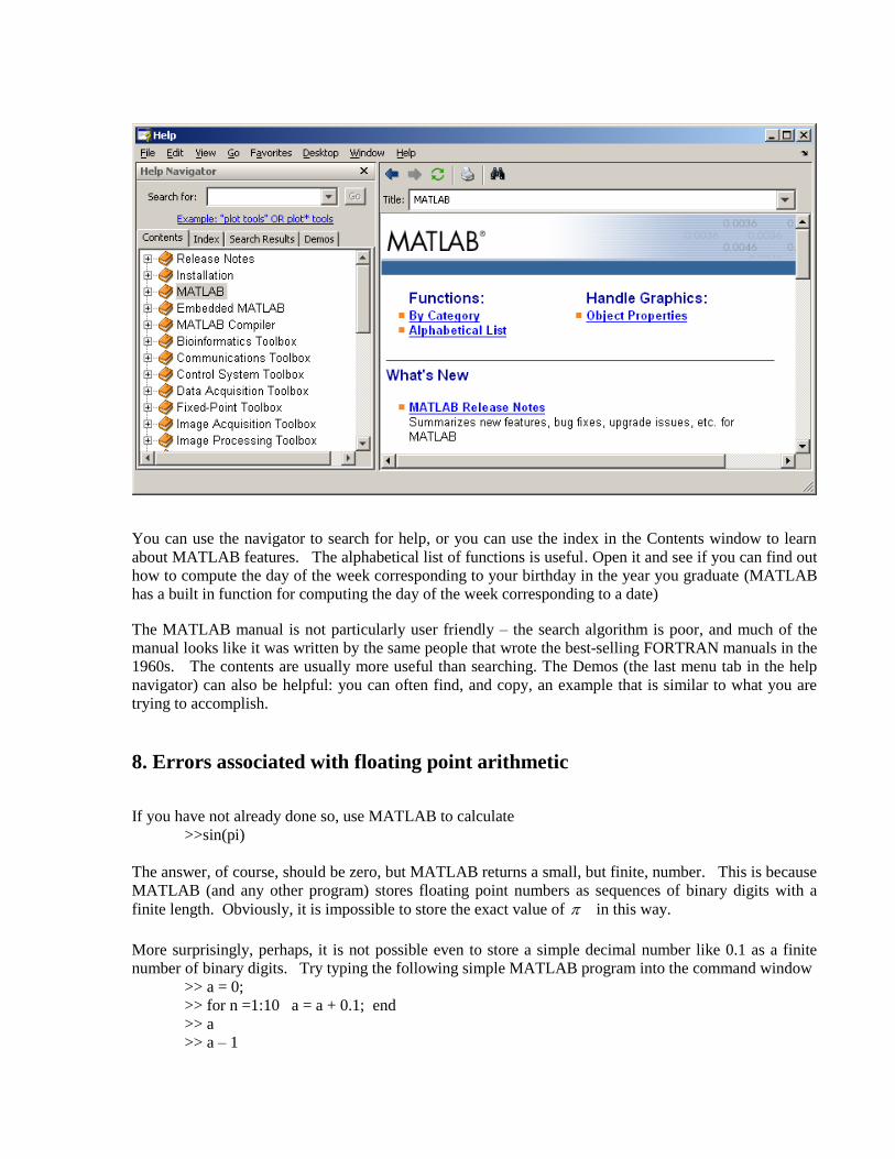
You can use the navigator to search for help, or you can use the index in the Contents window to learn

about MATLAB features. The alphabetical list of functions is useful. Open it and see if you can find out

how to compute the day of the week corresponding to your birthday in the year you graduate (MATLAB

has a built in function for computing the day of the week corresponding to a date)

The MATLAB manual is not particularly user friendly – the search algorithm is poor, and much of the

manual looks like it was written by the same people that wrote the best-selling FORTRAN manuals in the

1960s. The contents are usually more useful than searching. The Demos (the last menu tab in the help

navigator) can also be helpful: you can often find, and copy, an example that is similar to what you are

trying to accomplish.

8. Errors associated with floating point arithmetic

If you have not already done so, use MATLAB to calculate

>>sin(pi)

The answer, of course, should be zero, but MATLAB returns a small, but finite, number. This is because

MATLAB (and any other program) stores floating point numbers as sequences of binary digits with a

finite length. Obviously, it is impossible to store the exact value of in this way.

More surprisingly, perhaps, it is not possible even to store a simple decimal number like 0.1 as a finite

number of binary digits. Try typing the following simple MATLAB program into the command window

>> a = 0;

>> for n =1:10 a = a + 0.1; end

>> a

>> a – 1

Here, the line that reads “for n=1:10 a= a + 0.1; end” is called a “loop.” This is a very common operation

in most computer programs. It can be interpreted as the command: “for each of the discrete values of the

integer variable n between 1 and 10 (inclusive), calculate the variable “a” by adding +0.1 to the previous

value of “a” The loop starts with the value n=1 and ends with n=10.

Thus, the for… end loop therefore adds 0.1 to the variable a ten times. It gives an answer that is

approximately 1. But when you compute a-1, you don‟t end up with zero.

Of course -1.1102e-016 is not a big error compared to 1, and this kind of accuracy is good enough for

government work. But if someone subtracted 1.1102e-016 from your bank account every time a

financial transaction occurred around the world, you would burn up your bank account pretty fast.

Perhaps even faster than you do by paying your tuition bills.

You can minimize errors caused by floating point arithmetic by careful programming, but you can‟t

eliminate them altogether. As a user of MATLAB they are mostly out of your control, but you need to

know that they exist, and try to check the accuracy of your computations as carefully as possible.

9. Vectors in MATLAB

MATLAB can do all vector operations completely painlessly. Try the following commands

>> a = [6,3,4]

>> a(1)

>> a(2)

>> a(3)

>> b = [3,1,-6]

>> c = a + b

>> c = dot(a,b)

>> c = cross(a,b)

Calculate the magnitude of c (you should be able to do this with a dot product. MATLAB also has a

built-in function called `norm‟ that calculates the magnitude of a vector)

A vector in MATLAB need not be three dimensional. For example, try

>>a = [9,8,7,6,5,4,3,2,1]

>>b = [1,2,3,4,5,6,7,8,9]

You can add, subtract, and evaluate the dot product of vectors that are not 3D, but you can‟t take a cross

product. Try the following

>> a + b

>> dot(a,b)

>>cross(a,b)

In MATLAB, vectors can be stored as either a row of numbers, or a column of numbers. So you could

also enter the vector a as

>>a = [9;8;7;6;5;4;3;2;1]

to produce a column vector.

You can turn a row vector into a column vector, and vice-versa by

>> b = transpose(b)

A few more very useful vector tricks are:

You can create a vector containing regularly spaced data points very quickly with a loop. Try

>> for i=1:11 v(i)=0.1*(i-1); end

>> v

The for…end loop repeats the calculation with each value of i from 1 to 11. Here, the “counter”

variable i now is used to refer to the ith entry in the vector v, and also is used in the formula itself.

If you type

>> sin(v)

MATLAB will compute the sin of every number stored in the vector v and return the result as

another vector. This is useful for plots – see section 11.

You have to be careful to distinguish between operations on a vector (or matrix, see later) and

operations on the components of the vector. For example, try typing

>> v^2

This will cause MATLAB to bomb, because the square of a row vector is not defined. But you

can type

>> v.^2

(there is a period after the v, and no space). This squares every element within v. You can also

do things like

>> v. /(1+v)

(see if you can work out what this does).

I personally avoid using the dot notation – it is very confusing, and makes code hard to read.

Instead, I generally do operations on vector elements using loops. For example, instead of

writing w = v.^2, I would use

>> for i=1:length(v) w(i) = v(i)^2; end

Here, „for i=1:length(v)‟ repeats the calculation for every element in the vector v. The function

length(vector) determines how many components the vector v has (11 in this case).

10. Matrices in MATLAB

Hopefully you know what a matrix is… If not, it doesn‟t matter - you can read a summary of matrices

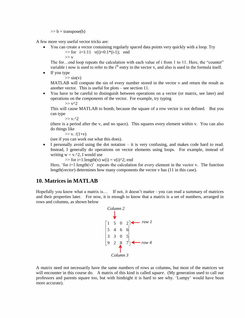
and their properties later. For now, it is enough to know that a matrix is a set of numbers, arranged in

rows and columns, as shown below

1 5 0 2

5 4 6 6

3 3 0 5

9 2 8 7

row 1

Column 2

row 4

Column 3

A matrix need not necessarily have the same numbers of rows as columns, but most of the matrices we

will encounter in this course do. A matrix of this kind is called square. (My generation used to call our

professors and parents square too, but with hindsight it is hard to see why. „Lumpy‟ would have been

more accurate).

You can create a matrix in MATLAB by entering the numbers one row at a time, separated by

semicolons, as follows

>> A = [1,5,0,2; 5,4,6,6;3,3,0,5;9,2,8,7]

You can extract the numbers from the matrix using the convention A(row #, col #). Try

>>A(1,3)

>>A(3,1)

You can also assign values of individual array elements

>>A(1,3)=1000

There are some short-cuts for creating special matrices. Try the following

>>B = ones(1,4)

>>C = pascal(6)

>>D = eye(4,4)

>>E = zeros(3,3)

The „eye‟ command creates the „identity matrix‟ – this is the matrix version of the number 1. You can

use

>> help pascal

to find out what pascal does.

MATLAB can help you do all sorts of things to matrices, if you are the sort of person that enjoys doing

things to matrices. Some of the things you can do to matrices are described in the intro to matrices. For

example

1. You can flip rows and columns with >> B = transpose(A)

2. You can add matrices (provided they have the same number of rows and columns >> C=A+B

Try also >> C – transpose(C)

A matrix that is equal to its transpose is called symmetric

3. You can multiply matrices – this is a rather complicated operation, which is described in detail in

the matrix tutorial. But in MATLAB you need only to type >>D=A*B to find the product of A

and B. Also try the following

>> E=A*B-B*A

>> F = eye(4,4)*A - A

4. You can do titillating things like calculate the determinant of a matrix; the inverse of a matrix, the

eigenvalues and eigenvectors of a matrix. If you want to try these things

>> det(A)

>> inv(A)

>> eig(A)

>> [W,D] = eig(A)

You can find out more about these functions, and also get a full list of MATLAB matrix

operations in the section of Help highlighted below

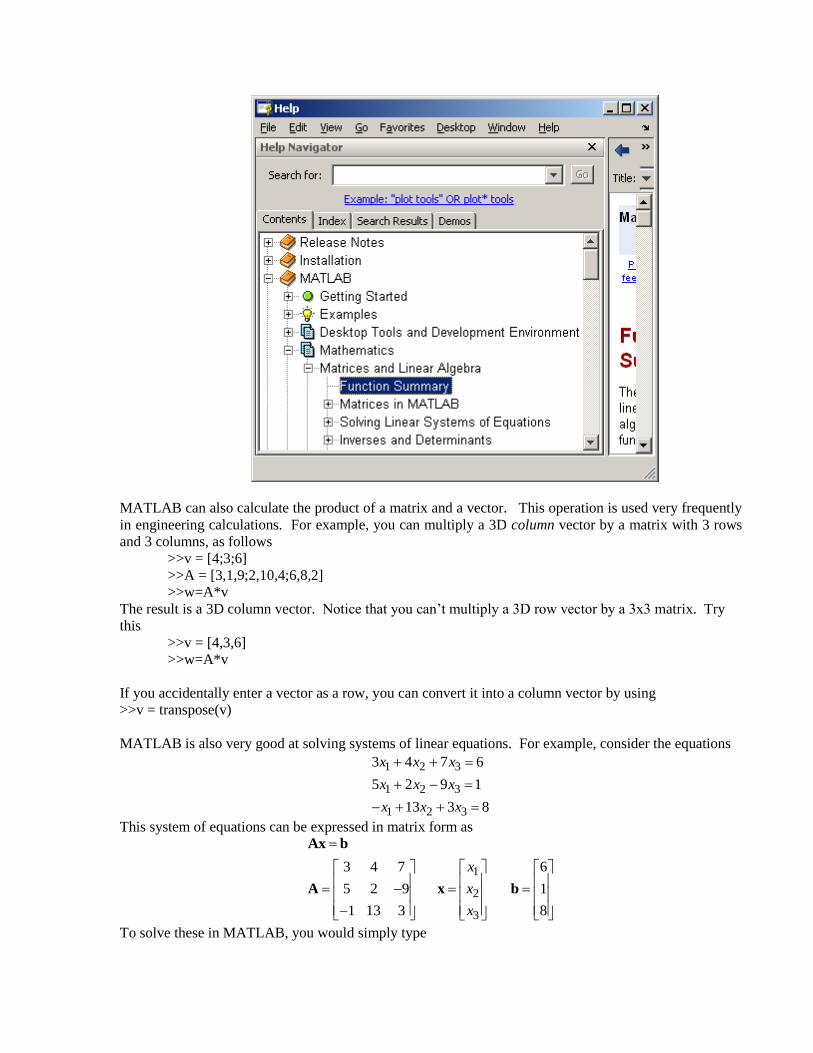
MATLAB can also calculate the product of a matrix and a vector. This operation is used very frequently

in engineering calculations. For example, you can multiply a 3D column vector by a matrix with 3 rows

and 3 columns, as follows

>>v = [4;3;6]

>>A = [3,1,9;2,10,4;6,8,2]

>>w=A*v

The result is a 3D column vector. Notice that you can‟t multiply a 3D row vector by a 3x3 matrix. Try

this

>>v = [4,3,6]

>>w=A*v

If you accidentally enter a vector as a row, you can convert it into a column vector by using

>>v = transpose(v)

MATLAB is also very good at solving systems of linear equations. For example, consider the equations

1 2 3

1 2 3

1 2 3

3 4 7 6

5 2 9 1

13 3 8

x x x

x x x

x x x

This system of equations can be expressed in matrix form as

1

2

3

3 4 7 6

5 2 9 1

1 13 3 8

x

x

x

Ax b

A x b

To solve these in MATLAB, you would simply type

>> A = [3,4,7;5,2,-9;-1,13,3]

>> b = [6;1;8]

>> x = A\b

(note the forward-slash, not the back-slash or divide sign) You can check your answer by calculating

>> A*x

The notation here is supposed to tell you that x is b „divided‟ by A – although `division‟ by a matrix has

to be interpreted rather carefully. Try also

>>x=transpose(b)/A

The notation transpose(b)/A solves the equations xA b , where x and b are row vectors. Again, you can

check this with

>>x*A

(The answer should equal b, (as a row vector) of course)

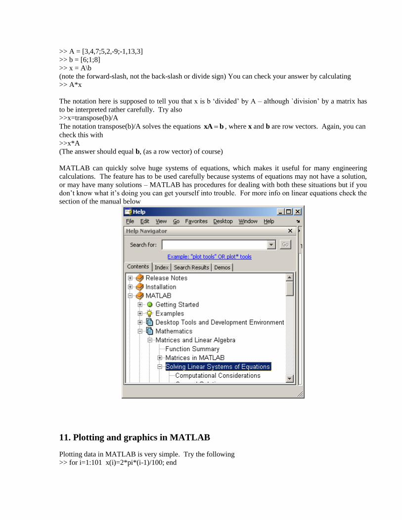
MATLAB can quickly solve huge systems of equations, which makes it useful for many engineering

calculations. The feature has to be used carefully because systems of equations may not have a solution,

or may have many solutions – MATLAB has procedures for dealing with both these situations but if you

don‟t know what it‟s doing you can get yourself into trouble. For more info on linear equations check the

section of the manual below

11. Plotting and graphics in MATLAB

Plotting data in MATLAB is very simple. Try the following

>> for i=1:101 x(i)=2*pi*(i-1)/100; end

>> y = sin(x)

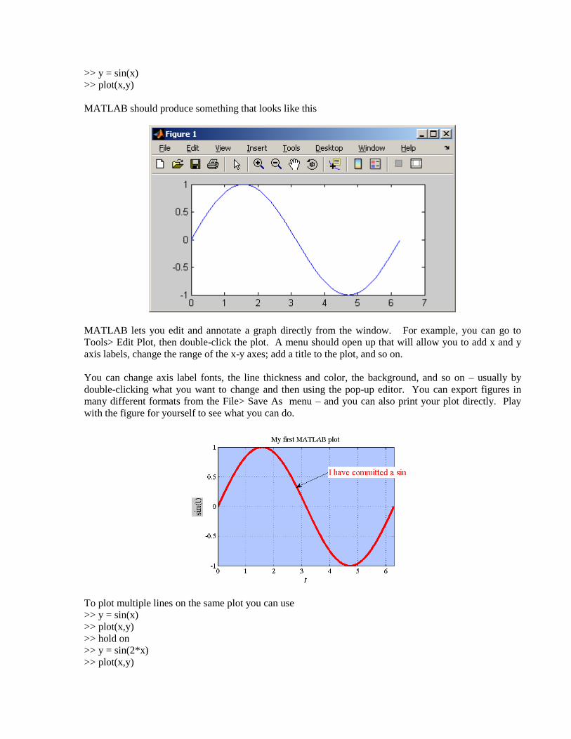
>> plot(x,y)

MATLAB should produce something that looks like this

MATLAB lets you edit and annotate a graph directly from the window. For example, you can go to

Tools> Edit Plot, then double-click the plot. A menu should open up that will allow you to add x and y

axis labels, change the range of the x-y axes; add a title to the plot, and so on.

You can change axis label fonts, the line thickness and color, the background, and so on – usually by

double-clicking what you want to change and then using the pop-up editor. You can export figures in

many different formats from the File> Save As menu – and you can also print your plot directly. Play

with the figure for yourself to see what you can do.

To plot multiple lines on the same plot you can use

>> y = sin(x)

>> plot(x,y)

>> hold on

>> y = sin(2*x)

>> plot(x,y)

Alternatively, you can use

>> y(1,:) = sin(x);

>> y(2,:) = sin(2*x);

>> y(3,:) = sin(3*x);

>> plot(x,y)

Here, y is a matrix. The notation y(1,:) fills the first row of y, y(2,:) fills the second, and so on. The

colon : ensures that the number of columns is equal to the number of terms in the vector x. If you prefer,

you could accomplish the same calculation in a loop:

>> for i=1:length(x) y(1,i) = sin(x(i)); y(2,i) = sin(2*x(i)); y(3,i) = sin(3*x(i)); end

>> plot(x,y)

Notice that when you make a new plot, it always wipes out the old one. If you want to create a new plot

without over-writing old ones, you can use

>> figure

>> plot(x,y)

The „figure‟ command will open a new window and will assign a new number to it (in this case, figure 2).

If you want to go back and re-plot an earlier figure you can use

>> figure(1)

>> plot(x,y)

If you like, you can display multiple plots in the same figure, by typing

>> newaxes = axes;

>> plot(x,y)

The new plot appears over the top of the old one, but you can drag it away by clicking on the arrow tool

and then clicking on any axis or border of new plot. You can also re-size the plots in the figure window

to display them side by side. The statement „newaxes = axes‟ gives a name (or „handle‟) to the new axes,

so you can select them again later. For example, if you were to create a third set of axes

>> yetmoreaxes = axes;

>> plot(x,y)

you can then go back and re-plot `newaxes‟ by typing

>> axes(newaxes);

>> plot(x,y)

Doing parametric plots is easy. For example, try

>> for i=1:101 t(i) = 2*pi*(i-1)/100; end

>> x = sin(t);

>> y = cos(t);

>> plot(x,y)

MATLAB has vast numbers of different 2D and 3D plots. For example, to draw a filled contour plot of

the function sin(2 )sin(2 )z x y for 0 1, 0 1x y , you can use

>> for i =1:51 x(i) = (i-1)/50; y(i)=x(i); end

>> z = transpose(sin(2*pi*y))*sin(2*pi*x);

>> figure

>> contourf(x,y,z)

The first two lines of this sequence should be familiar: they create row vectors of equally spaced points.

The third needs some explanation – this operation constructs a matrix z, whose rows and columns satisfy

z(i,j) = sin(2*pi*y(i)) * sin(2*pi*x(j)) for each value of x(i) and y(j).

If you like, you can change the number of contour levels

>>contourf(x,y,z,15)

You can also plot this data as a 3D surface using

>> surface(x,y,z)

The result will look a bit strange, but you can click on the „rotation 3D‟ button (the little box with a

circular arrow around it ) near the top of the figure window, and then rotate the view in the figure with

your mouse to make it look more sensible.

You can find out more about the different kinds of MATLAB plots in the section of the manual shown

below

12. Working with M files and defining new MATLAB functions

So far, we‟ve run MATLAB by typing into the command window. This is OK for simple calculations,

but usually it is better to type the list of commands you plan to execute into a file (called an M-file), and

then tell MATLAB to run all the commands together. One benefit of doing this is that you can fix errors

easily by editing and re-evaluating the file. But more importantly, you can use M-files to write simple

programs and functions using MATLAB.

To create an M-file, simply go to File > New > M-file on the main desktop menu. The m-file editor

will open, and show an empty file.

Type the following lines into the editor: for i=1:101

theta(i) = -pi + 2*pi*(i-1)/100;

rho(i) = 2*sin(5*theta(i));

end

figure

polar(theta,rho)

You can make MATLAB execute these statements by:

1. Pressing the green arrow near the top of the editor window – this will first save the file

(MATLAB will prompt you for a file name – save the script in a file called myscript.m), and will

then execute the file.

2. You can save the file yourself (e.g. in a file called myscript.m). You can then run the script from

the command window, by typing

>> myscript

You don‟t have to use the MATLAB editor to create M-files – any text editor will work. As long as you

save the file in plain text (ascii) format in a file with a .m extension, MATLAB will be able to find and

execute the file. To do this, you must open the directory containing the file with MATLAB (e.g. by

entering the path in the field at the top of the window). Then, typing

>> filename

in the command window will execute the file. Usually it‟s more convenient to use the MATLAB editor -

but if you happen to be stuck somewhere without access to MATLAB this is a useful alternative. (Then

again, this means you can‟t plead lack of access to MATLAB to avoid doing homework, so maybe there

is a down-side)

You can also use M-files to define new MATLAB functions – these are programs that can accept user-

defined data and use it to produce a new result. For example, to create a function that computes the

magnitude of a vector:

1. Open a new M-file with the editor

2. Type the following into the M-file function y = magnitude(v) % Function to compute the magnitude of a vector y = sqrt(dot(v,v)); end

Note that MATLAB ignores any lines that start with a % - this is to allow you to type comments

into your programs that will help you, or users of your programs, to understand them.

3. Save the file (accept the default file name, which is magnitude.m)

4. Type the following into the command window

>> v = [1,2,3];

>> magnitude(v)

You should find that this computes the magnitude of v correctly.

Note the syntax for defining a function – it must always have the form

function solution_variable = function_name(input_variables…)

…script consisting of commands needed to compute the function, ending with the

command:

solution_variable = ….

end

If you are writing functions for other people to use, it is a good idea to provide some help for the function,

and some error checking to stop users doing stupid things. MATLAB treats the comment lines that

appear just under the function name in a function as help, so if you type

>> help magnitude

into the command window, MATLAB will tell you what `magnitude‟ does. You could also edit the

program a bit to make sure that v is a vector, as follows function y = magnitude(v) % Function to compute the magnitude of a vector

% Check that v is a vector [m,n] = size(v); % [m,n] are the number of rows and columns of v % The next line checks if both m and n are >1, in which case v is

% a matrix, or if both m=1 and n=1, in which case v scalar; if either, % an error is returned if ( ( (m > 1) & (n > 1) ) | (m == 1 & n == 1) ) error('Input must be a vector') end y = sqrt(dot(v,v)); end

This program shows another important programming concept. The “if……end” set of commands is

called a “conditional” statement. You use it like this:

if (a test)

calculation to do if the test is true end

In this case the calculation is only done if test is true – otherwise the calculation is skipped altogether.

You can also do

if (a test)

calculation to do if the test is true else

calculation to do if the test is false end

In the example (m > 1) & (n > 1) means “m>1 and n>1” while | (m == 1 & n == 1) means

“or m=1 and n=1”. The symbols & and | are shorthand for `and‟ and „or‟.

Functions can accept or return data as numbers, arrays, strings, or even more abstract data types. For

example, the program below is used by many engineers as a substitute for social skills function s = pickup(person) % function to say hello to someone cute s = [‘Hello ‘ person ‘ you are cute’]

beep; end

You can try this out with

>> pickup(„Janet‟)

(Janet happens to be my wife‟s name. If you are also called Janet please don‟t attach any significance to

this example)

You can also pass functions into other functions. For example, create an M-file with this program function plotit(func_to_plot,xmin,xmax,npoints) % plot a graph of a function of a single variable f(x)

% from xmin to xmax, with npoints data points for n=1:npoints x(n) = xmin + (xmax-xmin)*(n-1)/(npoints-1); v(n) = func_to_plot(x(n)); end figure; plot(x,v);

end

Then save the M-file, and try plotting a cosine, by using

>> plotit(@cos,0,4*pi,100)

Several new concepts have been introduced here – firstly, notice that variables (like func_to_plot in this

example) don‟t necessarily have to contain numbers, or even strings. They can be more complicated

things called “objects.” We won‟t discuss objects and object oriented programming here, but the example

shows that a variable can contain a function. To see this, try the following

>> v = @exp

>> v(1)

This assigns the exponential function to a variable called v – which then behaves just like the exponential

function. The „@‟ before the exp is called a „function handle‟ – it tells MATLAB that the function

exp(x), should be assigned to v, instead of just a variable called exp.

The command “plotit(@cos,0,4*pi,100)” assigns the cosine function to the variable called func_to_plot.

Although MATLAB is not really intended to be a programming language, you can use it to write some

quite complicated code, and it is widely used by engineers for this purpose. CS4 will give you a good

introduction to MATLAB programming. But if you want to write a real program you should use a

genuine programming language, like C, C++, Java, lisp, etc.

13. Organizing complicated calculations as functions in an M file

It can be very helpful to divide a long and complicated calculation into a sequence of smaller ones, which

are done by separate functions in an M file. As a very simple example, the M file shown below creates

plots a pseudo-random function of time, then computes the root-mean-square of the signal. Copy and

paste the example into a new MATLAB M-file, and press the green arrow to see what it does.

function randomsignal

% Function to plot a random signal and compute its RMS.

npoints = 100; % No. points in the plot

dtime = 0.01; % Time interval between points

% Compute vectors of time and the value of the function.

% This example shows how a function can calculate several

% things at the same time.

[time,function_value] = create_random_function(npoints,dtime);

% Compute the rms value of the function

rms = compute_rms(time,function_value);

% Plot the function

plot(time,function_value);

% Write the rms value as a label on the plot

label = strcat('rms signal = ',num2str(rms));

annotation('textbox','String',{label},'FontSize',16,...

'BackgroundColor',[1 1 1],...

'Position',[0.3499 0.6924 0.3944 0.1]);

end

%

function [t,y] = create_random_function(npoints,time_interval)

% Create a vector of equally spaced times t(i), and

% a vector y(i), of random values with i=1…npoints

for i = 1:npoints

t(i) = time_interval*(i-1);

% The rand function computes a random number between 0 and 1

y(i) = rand-0.5;

end

end

function r = compute_rms(t,y)

% Function to compute the rms value of a function y of time t.

% t and y are both vectors

for i = 1:length(y)

ysquared(i) = y(i)*y(i);

end

% The trapz function uses a trapezoidal integration

% method to compute the integral of a function.

integral = trapz(t,ysquared);

r = sqrt(integral/t(length(t))); % This is the rms.

end

Some remarks on this example:

1. Note that the m-file is organized as

main function – this does the whole calculation

result 1 = function1(data)

result2 = function2(data)

end of main function

Definition of function 1

Definition of function2

When you press the green arrow to execute the M file, MATLAB will execute all the statements

that appear in the main function. The statements in function1 and function2 will only be

executed if the function is used inside the main function; otherwise they just sit there waiting to

be asked to do something. I remember doing much the same thing at high-school dances.

2. When functions follow each other in sequence, as shown in this example, then variables defined

in one function are invisible to all the other functions. For example, the variable „integral‟ only

has a value inside the function compute_rms. It does not have a value in create_random_value.

14. Solving differential equations with MATLAB

The main reason for learning MATLAB in EN40 is so you can use it to analyze motion of an engineering

system. To do this, you always need to solve a differential equation. MATLAB has powerful numerical

methods to solve differential equations. They are best illustrated by means of examples.

14.1 Solving a basic differential equation.

Suppose we want to solve the equation

10 sin( )dy

y tdt

with initial conditions 0y at time t=0. We are interested in calculating y as a function of time – say

from time t=0 to t=20. We won‟t actually compute a formula for y – instead, we calculate the value of y

at a series of different times in this interval, and then plot the result.

We would do this as follows

1. Create a function (in an m-file) that calculates dy

dt, given values of y and t. Create an m-file as

follows, and save it in a file called „simple_ode.m‟ function dydt = simple_ode(t,y) % Example of a MATLAB differential equation function

dydt = -10*y + sin(t); end

2. To see what this function does, try typing the following into the MATLAB command window.

>> simple_ode(0,0)

>> simple_ode(0,1)

>> simple_ode(pi/2,0)

For these three examples, the function returns the value of /dy dt for (t=0,y=0); (t=0,y=1) and

(t=pi,y=0), respectively. Do the calculation in your head to check that the function is working.

3. Now, you can tell MATLAB to solve the differential equation for y and plot the solution using

>> [t_values,y_values] = ode45(@simple_ode,[0,20],0);

>> plot(t_values,y_values)

Here,

ode45(@function name,[start time, end time], initial condition for variable y)

is a special MATLAB function that will integrate the differential equation (numerically). Note that a

`function handle‟ (the @) has to be used to tell MATLAB the name of the function to be integrated.

Your graph should look like the plot shown below

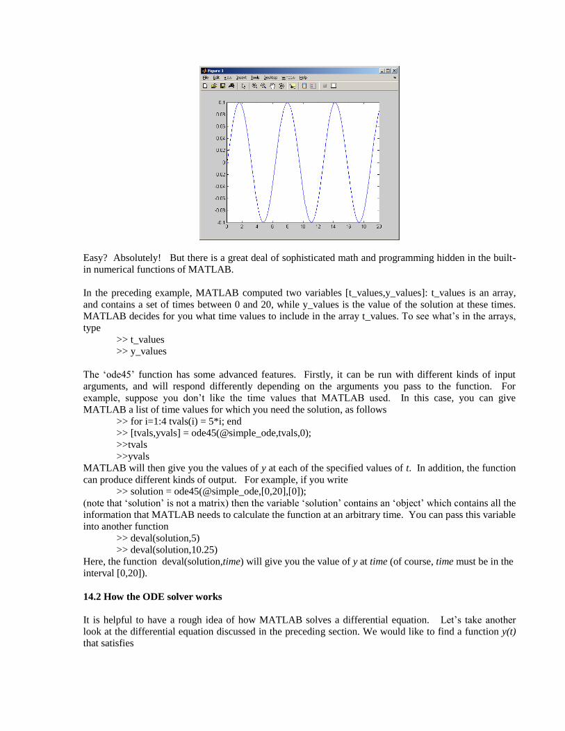
Easy? Absolutely! But there is a great deal of sophisticated math and programming hidden in the built-

in numerical functions of MATLAB.

In the preceding example, MATLAB computed two variables [t_values,y_values]: t_values is an array,

and contains a set of times between 0 and 20, while y_values is the value of the solution at these times.

MATLAB decides for you what time values to include in the array t_values. To see what‟s in the arrays,

type

>> t_values

>> y_values

The „ode45‟ function has some advanced features. Firstly, it can be run with different kinds of input

arguments, and will respond differently depending on the arguments you pass to the function. For

example, suppose you don‟t like the time values that MATLAB used. In this case, you can give

MATLAB a list of time values for which you need the solution, as follows

>> for i=1:4 tvals(i) = 5*i; end

>> [tvals,yvals] = ode45(@simple_ode,tvals,0);

>>tvals

>>yvals

MATLAB will then give you the values of y at each of the specified values of t. In addition, the function

can produce different kinds of output. For example, if you write

>> solution = ode45(@simple_ode,[0,20],[0]);

(note that „solution‟ is not a matrix) then the variable „solution‟ contains an „object‟ which contains all the

information that MATLAB needs to calculate the function at an arbitrary time. You can pass this variable

into another function

>> deval(solution,5)

>> deval(solution,10.25)

Here, the function deval(solution,time) will give you the value of y at time (of course, time must be in the

interval [0,20]).

14.2 How the ODE solver works

It is helpful to have a rough idea of how MATLAB solves a differential equation. Let‟s take another

look at the differential equation discussed in the preceding section. We would like to find a function y(t)

that satisfies

10 sin( )dy

y tdt

with 0y at time t=0. We won‟t attempt to find an algebraic formula for y – instead, we will just

compute the value of y at a series of different times between 0t and 20t - say 0, 0.1, 0.2...t t t

To see how to do this, remember the definition of a derivative

0

( ) ( )limt

dy y t t y t

dt t

So if we know the values of y and /dy dt at some time t, we can use this formula backwards to calculate

the value of y at a slightly later time t t

( ) ( )dy

y t t y t tdt

This procedure can be repeated to find all the values of y we need. We can do the calculation in a small

loop. Try typing the function below in a new M-file, and run it to see what it does. function simple_ode_solution

% The initial values of y and t

y(1) = 0;

t(1) = 0;

delta_t = 0.1;

n_steps = 20/delta_t;

for i = 1:n_steps

dydt = -10*y(i) + sin(t(i)); % Compute the derivative

y(i+1) = y(i) + delta_t*dydt; % Find y at time t+delta_t

t(i+1) = t(i) + delta_t; % Store the time

end

plot(t,y);

end

Now, we can use this idea to write a more general function that behaves like the MATLAB ode45()

function for solving an arbitrary differential equation. Cut and paste the code below into a new M-file,

and then save it in a file called my_ode_solver. function [t,y] = my_ode_solver(ode_function,time_int,initial_y)

y(1) = initial_y;

t(1) = time_int(1);

n_steps = 200;

delta_t = (time_int(2)-time_int(1))/n_steps;

for i = 1:n_steps

dydt = ode_function(t(i),y(i));% Compute the derivative

y(i+1) = y(i) + delta_t*dydt;% Find y at time t+delta_t

t(i+1) = t(i) + delta_t;% Store the time

end

end

You can now use this function just like the built-in MATLAB ODE solver. Try it by typing

>> [t_values,y_values] = my_ode_solver(@simple_ode,[0,20],0);

>> plot(t_values,y_values)

into the MATLAB command window (if you get an error, make sure your simple_ode function defined in

the preceding section is stored in the same directory as the function my_ode_solver).

Of course, the MATLAB equation solver is actually much more sophisticated than this simple code, but it

is based on the same idea.

14.3 Solving a differential equation with adjustable parameters.

For design purposes, we often want to solve equations which include design parameters. For example, we

might want to solve

sin( )dy

ky F tdt

with different values of k, F and , so we can explore how the system behaves. It would be nice to be

able to pass these parameters to the function `simple_ode‟, for example by using function dydt = simple_ode(t,y,k,F,omega) % Example of a MATLAB differential equation function dydt = -k*y + F*sin(omega*t); end

but this doesn’t work – don‟t bother trying. Instead, you have to make the function simple_ode, a nested

function within an M-file, as follows. Open a new M-file, and type (or cut and paste) the following

example function solve_my_ode % Function to solve dy/dt = -k*y + F*sin(omega*t) % from t=tstart to t=tstop, with y(0) = initial_y

% Define parameter values below. k = 10;

F = 1;

omega = 1;

tstart = 0;

tstop = 20;

initial_y = 0;

[times,sols] = ode45(@diff_equation,[tstart,tstop],initial_y);

plot(times,sols);

function dydt = diff_equation(t,y) % Function defining the ODE dydt = -k*y + F*sin(omega*t); end

end % Here is the end of the ‘solve my ode’ function

The function „diff_equation‟ is said to be nested within the function „solve_my_ode‟ because it appears

before the „end‟ statement that terminates the „solve_my_ode‟ function. Because the function is nested,

the variables (k,F,omega,tstart,tstop), which are given values in the _solve_my_ode function, have the

same values inside the diff_equation function. Note that variable values are only shared by nested

functions, not by functions that are defined in sequence.

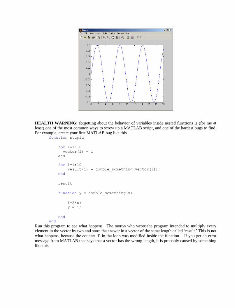
Now you can solve the ODE by executing the M-file. You can get solutions with different parameter

values quickly by editing the M-file.

Your graph should look like this

HEALTH WARNING: forgetting about the behavior of variables inside nested functions is (for me at

least) one of the most common ways to screw up a MATLAB script, and one of the hardest bugs to find.

For example, create your first MATLAB bug like this function stupid

for i=1:10

vector(i) = i

end

for i=1:10

result(i) = double_something(vector(i)); end

result

function y = double_something(x)

i=2*x; y = i;

end end

Run this program to see what happens. The moron who wrote the program intended to multiply every

element in the vector by two and store the answer in a vector of the same length called „result.‟ This is not

what happens, because the counter „i‟ in the loop was modified inside the function. If you get an error

message from MATLAB that says that a vector has the wrong length, it is probably caused by something

like this.

14.4 Solving simultaneous differential equations

Most problems in dynamics involve more complicated differential equations than those described in the

preceding section. Usually, we need to solve several differential equations at once – for example, if we

are interested in 3D motion, we would need to solve for 3 (x,y,z) components of position, or velocity, at

the same time. Fortunately MATLAB knows how to do this. As a simple example, let‟s write a function

to solve and plot the solution for the following pair of coupled ODEs

2 2 2 29.81yx

x x y y x y

dvdvcv v v cv v v

dt dt

with initial conditions 0 0cos sinx yv V v V , at time t=0, where c, 0V and are parameters.

(These happen to be the differential equations that govern the x and y components of velocity of a

projectile, accounting for the effects of air resistance). Before proceeding, make sure you are clear in

your mind what is being calculated – we want to find two functions of time ( ), ( )x yv t v t that satisfy the

two differential equations. As before, we won‟t compute the functions algebraically. Instead, we will

calculate values for ( ), ( )x yv t v t , at a sequence of successive times, and then plot the results.

To do this, we must first define a function that specifies the differential equations. This function must

calculate values for / , /x ydv dt dv dt given values of ,x yv v and time. The following function will do the

trick function dydt = ode_function(t,y)

vx = y(1);

vy = y(2);

vmag = sqrt(vx^2+vy^2);

dvxdt = -c*vx*vmag;

dvydt = -9.81-c*vy*vmag; dydt = [dvxdt;dvydt]; % Note the ;, which makes dydt a column vector

end

To understand how this works, note that when MATLAB is solving several ODEs, it stores the variables

as components of a vector. In this example, the variables ,x yv v are stored in a column vector y, with

components (1) xy v , (2) yy v . Similarly, the variables / , /x ydv dt dv dt are stored in a vector dydt,

with components (1) /xdydt dv dt and (2) /ydydt dv dt . So the function (i) extracts values for ,x yv v

out of the vector y; then (ii) uses these to compute values for / , /x ydv dt dv dt ; then (iii) sets up the

column vector dydt.

HEALTH WARNING: Note that the variable dydt computed by ode_function must be a column vector

(that‟s why semicolons appear between the dvxdt and the dvydt in the definition of dydt). If you forget to

do this, you will get a very confusing error message out of MATLAB.

Now, to solve the ODEs, create an M-file containing this function as shown below.

function solve_coupled_odes % Function to solve a vector valued ODE

V0 = 10;

theta = 45;

c=0.1;

tstart = 0;

tstop = 1.5;

theta = theta*pi/180; % convert theta to radians

%compute initial values for the two velocity components y0 = [V0*cos(theta);V0*sin(theta)]; % IF you like you can also specify the initial condition as a row

% eg using y0= [V0*cos(theta),V0*sin(theta)] – MATLAB will accept both.

%Here is the call for the ODE solver

[times,sols] = ode45(@odefunc,[tstart,tstop],y0);

plot(times,sols);

%here is the (vector) function to be integrated function dydt = ode_function(t,y)

vx = y(1);

vy = y(2);

vmag = sqrt(vx^2+vy^2);

dvxdt = -c*vx*vmag;

dvydt = -9.81-c*vy*vmag; dydt = [dvxdt;dvydt];

end

end

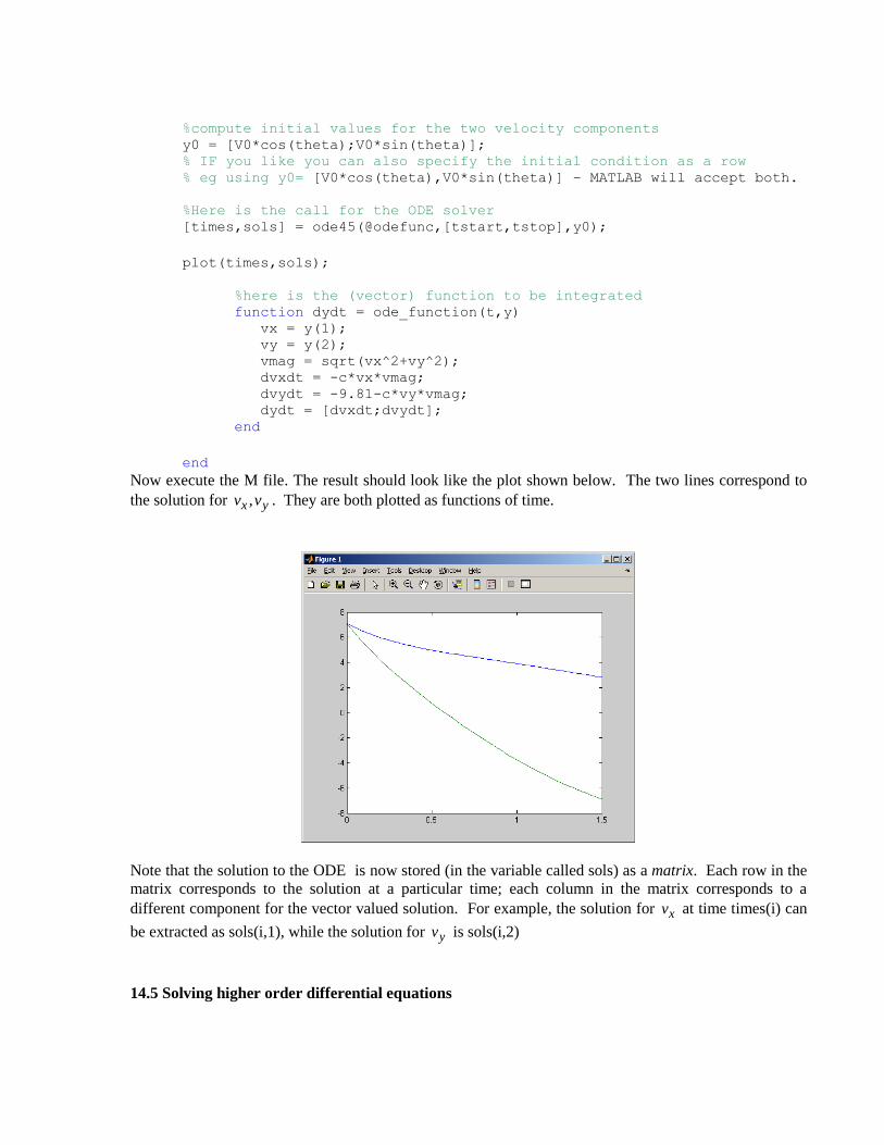
Now execute the M file. The result should look like the plot shown below. The two lines correspond to

the solution for ,x yv v . They are both plotted as functions of time.

Note that the solution to the ODE is now stored (in the variable called sols) as a matrix. Each row in the

matrix corresponds to the solution at a particular time; each column in the matrix corresponds to a

different component for the vector valued solution. For example, the solution for xv at time times(i) can

be extracted as sols(i,1), while the solution for yv is sols(i,2)

14.5 Solving higher order differential equations

The equations we solve in dynamics usually involve accelerations, and so don‟t have the form

/ ( , )d dt f ty y required by MATLAB. Fortunately, a simple trick can be used to convert an equation

involving accelerations into this form. As an example, suppose that we would like to plot the trajectory

of a projectile as it flies through the air, accounting for the effects of air resistance. The equations for the

(x,y) coordinates of the projectile are 2 2

2 2

d x dx d y dyc v g c v

dt dtdt dt

where c is the specific drag coefficient for the projectile ,g is the gravitational acceleration, and

2 2dx dy

vdt dt

is the magnitude of the velocity of the projectile. The initial conditions for the equation are

0 00 cos sindx dy

x y V Vdt dt

at time t=0. We would like to solve these equations for (x,y), but MATLAB can‟t handle the equations in

this form. To convert this into the correct form for MATLAB, we simply introduce new variables to

denote /dx dt and /dy dt

x ydx dy

v vdt dt

and note that 2 2

2 2

yxdvdvd x d y

dt dtdt dt

With these substitutions, our equations of motion become

yxx y

dvdvc v v g c v v

dt dt

We now have four unknowns [ , , , ]x yx y v vy , and can write the equation of motion as

x

y

x x

y y

vx

vyd

v c v vdt

v g c v v

This is now in standard MATLAB form, and you can solve it by making a small change to the

plot_vector_ode function, as follows function plot_vector_ode % Function to calculate and plot trajectory of a projectile

V0 = 10;

theta = 45;

c=0.1;

tstart = 0;

tstop = 1.5;


% w0 contains initial values for all four variables

% stored as [x,y,vx,vy] w0 = [0;0;V0*cos(theta);V0*sin(theta)];

% solve the ode for the output vector w as a function of time t:

[times,sols] = ode45(@odefunc,[tstart,tstop],w0);

% The solution is a matrix. Each row of the matrix contains

% [x,y,vx,vy] at a particular time. The next line plots

% x as a function of y.

plot(sols(:,1),sols(:,2));

function dwdt = odefunc(t,w)

% The vector w contains [x,y,v_x,v_y]. We start by extracting these

% Note that the argument of the function has been named w, because

% we use y for another variable. x = w(1);

y = w(2);

vx = w(3);

vy = w(4);

vmag = sqrt(vx^2+vy^2); dwdt = [vx;vy;-c*vx*vmag;-9.81-c*vy*vmag]; end

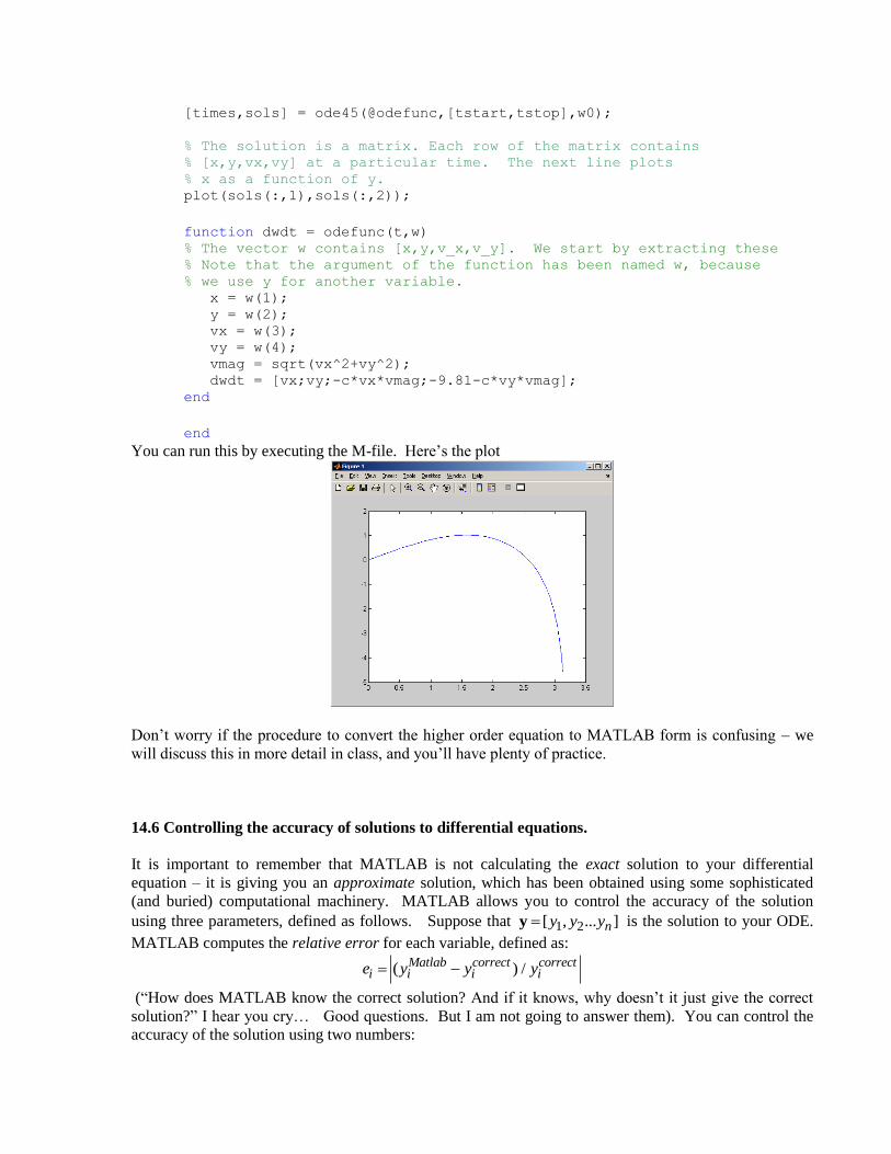
end

You can run this by executing the M-file. Here‟s the plot

Don‟t worry if the procedure to convert the higher order equation to MATLAB form is confusing – we

will discuss this in more detail in class, and you‟ll have plenty of practice.

14.6 Controlling the accuracy of solutions to differential equations.

It is important to remember that MATLAB is not calculating the exact solution to your differential

equation – it is giving you an approximate solution, which has been obtained using some sophisticated

(and buried) computational machinery. MATLAB allows you to control the accuracy of the solution

using three parameters, defined as follows. Suppose that 1 2[ , ... ]ny y yy is the solution to your ODE.

MATLAB computes the relative error for each variable, defined as:

( ) /Matlab correct correcti i i ie y y y

(“How does MATLAB know the correct solution? And if it knows, why doesn‟t it just give the correct

solution?” I hear you cry… Good questions. But I am not going to answer them). You can control the

accuracy of the solution using two numbers:

1. The absolute tolerance for each variable. This number specifies when each variable is small

enough to be taken to be zero. By default the absolute tolerance for all variables is 610

2. The relative tolerance. This number specifies the maximum allowable relative error in any

variable whose magnitude exceeds the absolute tolerance. The default value is 310 - i.e. 0.1%

You can set different values for each of these control parameters as shown in the code sample below

function plot_vector_ode % Function to plot the trajectory of a projectile

V0 = 10;

theta = 45;

c=0.1;

tstart = 0;

tstop = 1.5;

theta = theta*pi/180; % convert theta to radians w0 = [0;0;V0*cos(theta);V0*sin(theta)]; options = odeset('RelTol',0.00001,'AbsTol',[10^(-8),10^(-8),10^(-

8),10^(-8)]); [times,sols] = ode45(@odefunc,[tstart,tstop],w0,options);

figure plot(sols(:,1),sols(:,2));


% The vector w contains [x,y,v_x,v_y]. We start by extracting these x = w(1);

y = w(2);

vx = w(3);

vy = w(4);


end

Here, the „odeset(„variable name’,value,…) function is used to set values for special control variables in

the MATLAB differential equation solver. This example sets the relative tolerance to 510 and the

absolute tolerance for each variable to 810 . Note that you can only specify one value for the relative

tolerance, but you can specify an absolute tolerance for each variable separately. You might like to play

around with the values of these tolerances to see how they affect the solution.

14.7 Refining the solution if the step-size is too large in a plot.

Some ODEs are so simple and well-behaved that MATLAB can take huge time-steps. When this happens

you may get an ugly looking plot, even though the solution is still accurate. You can make MATLAB

smooth out the solution by setting a parameter called „refine.‟ To test this, try function plot_vector_ode % Function to plot the trajectory of a projectile

V0 = 10;

theta = 45;

c=0.1;

tstart = 0;

tstop = 1.5;

theta = theta*pi/180; % convert theta to radians w0 = [0;0;V0*cos(theta);V0*sin(theta)];

options = odeset('RelTol',0.01,'Refine',1); [times,sols] = ode45(@odefunc,[tstart,tstop],w0,options);




y = w(2);

vx = w(3);

vy = w(4);


end

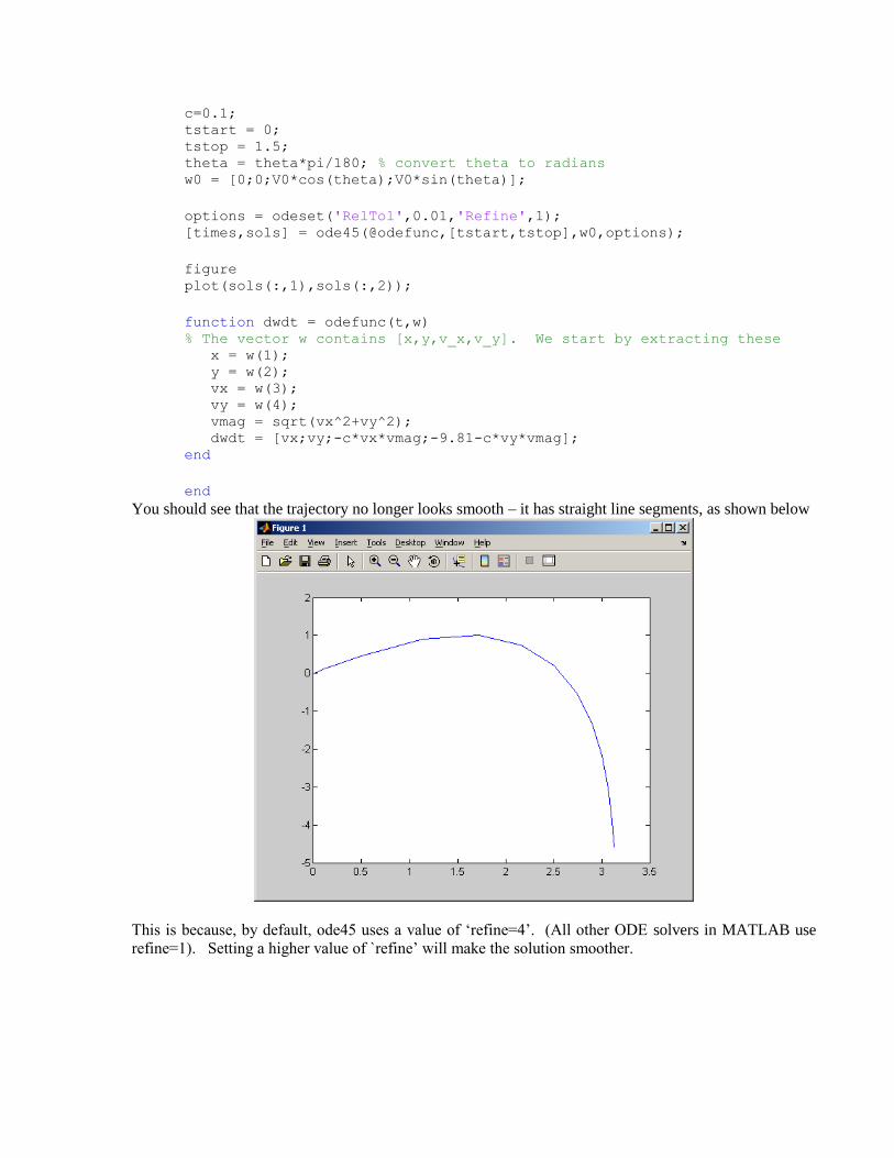
You should see that the trajectory no longer looks smooth – it has straight line segments, as shown below

This is because, by default, ode45 uses a value of „refine=4‟. (All other ODE solvers in MATLAB use

refine=1). Setting a higher value of `refine‟ will make the solution smoother.

14.8 Looking for special events in a solution

In many calculations, you aren‟t really interested in the time-history of the solution – instead, you are

interested in learning about something special that happens to the system. For example, in the trajectory

problem discussed in the preceding section, you might be interested in computing the maximum height

reached by the projectile, or the distance it travels. You can so this by adding an èvent‟ function to your

m-file. This procedure is best illustrated by examples.

Example1: stopping the trajectory calculation when the projectile returns to the ground. If you add the

function below to your `plot_vector_ode‟ script, it will continue the calculation until the projectile reaches

y=0, and then stop. Try it and see what happens. Note that you have to modify the òptions=‟ line as well

as adding the èvent‟ function. function plot_vector_ode

% Function to plot the trajectory of a projectile

V0 = 10;

theta = 45;

c=0.1;

tstart = 0;

tstop = 1.5;


options = odeset('Events',@events); [times,sols] = ode45(@odefunc,[tstart,tstop],w0,options);



% The vector w contains [x,y,v_x,v_y]. We start by extracting

these x = w(1);

y = w(2);

vx =w(3);

vy = w(4);

vmag = sqrt(vx^2+vy^2); dwdt = [vx;vy;-c*vx*vmag;-9.81-c*vy*vmag];

end

function [eventvalue,stopthecalc,eventdirection] = events(t,w) % Function to check for a special event in the trajectory % In this example, we look for the point when y=0 and % y is decreasing, and then stop the calculation. y = w(2) eventvalue = y; stopthecalc = 1; eventdirection = -1; end

end

Here is an explanation of what‟s happening in this example. To check for an „event‟ of some kind, you

have to feed a user-defined function to the ODE solver function ode45(). You do this by using

options=odeset(„Events‟,@events);

This tells MATLAB to use the function called èvents‟ to check for events. You could name the function

something else, if you prefer. The èvent‟ function must always return 3 variables, as shown in the

example, and they must always be in the correct order in the function name line. Here‟s what the

variables do:

1. „eventvalue‟ is a number that MATLAB will use to check for something you are interested in.

MATLAB will take action if it finds that èventvalue‟ reaches zero – otherwise it will simply

continue the calculation. Here, we are simply interested in finding when y=0. Recall that y is

stored in w(2).

2. „stopthecalc‟ tells MATLAB whether or not to continue the calculation if it detects the event. If

you set „stopthecalc=1‟ it will stop; otherwise if you set „stopthecalc=0‟ it will continue.

3. „eventdirection‟ gives you some additional control over event detection. In this particular

example, it is not enough to check for y=0 – the height of the projectile starts at y=0, so if we

only check for y=0 the calculation will never get anywhere. We are only interested in finding the

point where y=0 and y is decreasing. The èventdirection‟ number makes MATLAB respond as

follows

If èventdirection=0‟ MATLAB will respond each time „eventvalue=0‟

If „eventdirection=1‟ MATLAB will respond only when eventvalue=0 and is increasing

If „eventdirection=-1‟ MATLAB will respond only when eventvalue=0 and is decreasing.

Here‟s what happens if you run the script

Example 2: Making the projectile bounce when it hits the ground. Sometimes, we use èvents‟ to

change the way the solution behaves. For example, we might want to make our projectile bounce when it

hits the ground. You can‟t code this behavior into the equations of motion – you have to stop the

calculation, change the velocity of the projectile to make it bounce, and start the calculation again. Here‟s

how to modify your M-file to do this. function plot_vector_ode

% Function to plot the trajectory of a projectile V0 = 10;

theta = 45;

c=0.1;

tstart = 0;

tstop = 15;


w0 = [0;0;V0*cos(theta);V0*sin(theta)];

options = odeset('Events',@events);

max_number_bounces = 8; % The full solution will be stored in matrices times,sols times = 0; sols = transpose(w0);

for n = 1:max_number_bounces

[tbounce,wbounce] = ode45(@odefunc,[tstart,tstop],w0,options);

% This appends the solution for the nth bounce to the end of the full

solution n_steps = length(tbounce); % Extracts # of steps in new solution times = [times;tbounce(1:n_steps)]; % This appends the new times to

end of the existing ones sols = [sols;wbounce(1:n_steps,:)]; % This appends new solution to

end of y

% This sets the initial conditions for the next bounce w0 = wbounce(n_steps,:); % Initial condition is sol at end of bounce w0(4) = -w0(4); % But we change the direction of vertical velocity tstart = tbounce(n_steps);

end


etc...

The functions „odefunc‟ and „events‟ are not shown – they are the same as for the preceding example.

Here‟s the solution for this case

Example 3: Calculating the height of the projectile during each bounce. The èvent‟ function can also

be used to look for special features of the solution. Each time an èvent‟ is detected, MATLAB makes a

note of the time, and the value of the solution, and then returns this data when the computation is finished.

An example is shown in the script below. This script finds the time and height of the projectile at the top

of each successive bounce, and plots a graph of the max bounce height as a function of time. function plot_vector_ode % Function to plot the trajectory of a projectile V0 = 10;

theta = 45;

c=0.1;

tstart = 0;

tstop = 15;


options = odeset('Events',@events);

max_number_bounces = 8; % The full solution will be in times,sols times = 0; sols = transpose(w0); % These store the max height of each bounce, and the corresponding time maxheight = []; maxtime = []; for n = 1:max_number_bounces

[tbounce,wbounce,tevent,wevent,indexevent] =

ode45(@odefunc,[tstart,tstop],w0,options);

% This appends the solution for the nth bounce to the end of the full

solution n_steps = length(tbounce); times = [times;tbounce(1:n_steps)]; sols = [sols;wbounce(1:n_steps,:)];

% This finds the event corresponding to the max height of the bounce % The index for this event is (2) (because its the second one listed % in the èvent' function n_events = length(tevent); for n=1:n_events if (indexevent(n)==2) maxheight = [maxheight,wevent(n,2)]; maxtime = [maxtime,tevent(n)]; end end

% This sets the initial conditions for the next bounce w0 = wbounce(n_steps,:); w0(4) = -w0(4); tstart = tbounce(n_steps);

end

figure('Units','pixels','Position',[250,250,800,400]); axes1 = subplot(1,2,1); plot(sols(:,1),sols(:,2));

axes2 = subplot(1,2,2); plot(maxtime,maxheight);



y = w(2);

vx =w(3);

vy = w(4);

vmag = sqrt(vx^2+vy^2); dwdt = [vx;vy;-c*vx*vmag;-9.81-c*vy*vmag];

end

function [eventvalue,stopthecalc,eventdirection] = events(t,w) % Function to check for a special event in the trajectory % In this example, we look % (1) for the point when y=0 and y is decreasing. % (2) for the point where vy=0 (the top of the bounce)

y = w(2);

vy = w(4);

eventvalue = [y,vy]; stopthecalc = [1,0]; eventdirection = [-1,0]; end

end

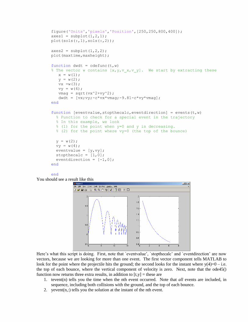
You should see a result like this

Here‟s what this script is doing. First, note that `eventvalue‟, `stopthecalc‟ and `eventdirection‟ are now

vectors, because we are looking for more than one event. The first vector component tells MATLAB to

look for the point where the projectile hits the ground; the second looks for the instant where y(4)=0 – i.e.

the top of each bounce, where the vertical component of velocity is zero. Next, note that the ode45()

function now returns three extra results, in addition to [t,y] = these are

1. tevent(n) tells you the time when the nth event occurred. Note that all events are included, in

sequence, including both collisions with the ground, and the top of each bounce.

2. yevent(n,:) tells you the solution at the instant of the nth event.

3. indexevent(n) tells you what happened at the nth event – if indexevent(n)=1, it is a bounce, if

indexevent(n)=2, it is the instant of max height.

The rest of the script is just data management.

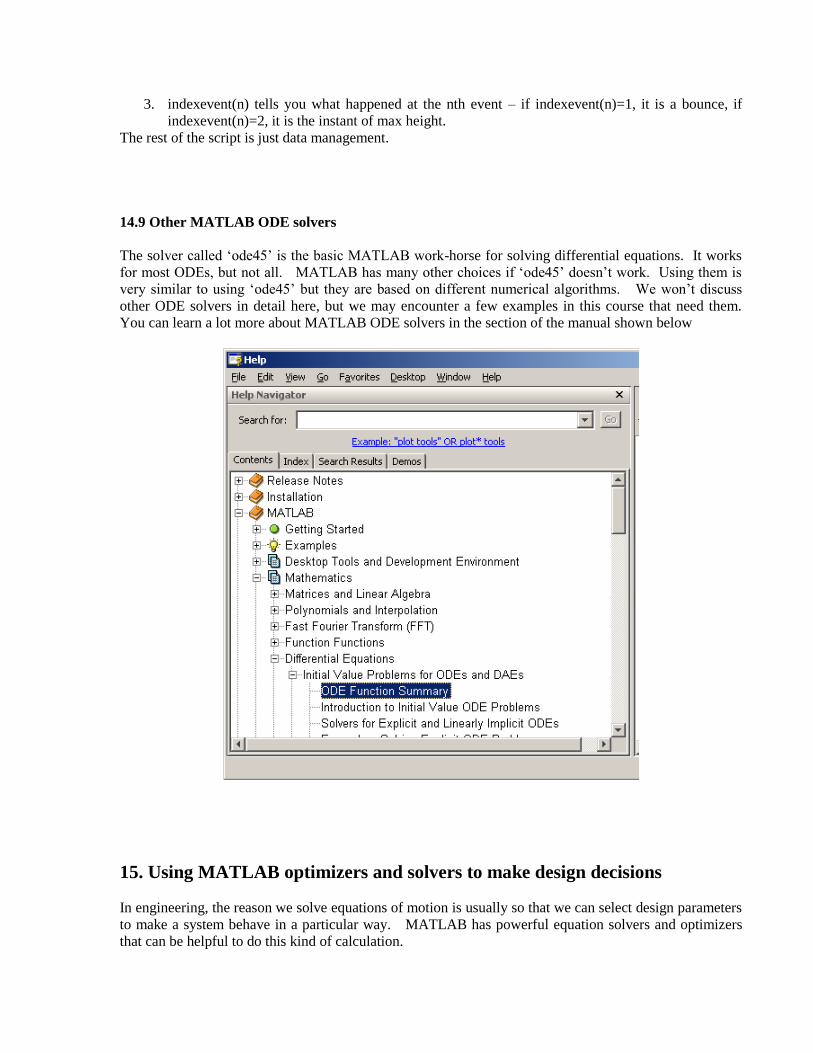
14.9 Other MATLAB ODE solvers

The solver called „ode45‟ is the basic MATLAB work-horse for solving differential equations. It works

for most ODEs, but not all. MATLAB has many other choices if „ode45‟ doesn‟t work. Using them is

very similar to using „ode45‟ but they are based on different numerical algorithms. We won‟t discuss

other ODE solvers in detail here, but we may encounter a few examples in this course that need them.

You can learn a lot more about MATLAB ODE solvers in the section of the manual shown below

15. Using MATLAB optimizers and solvers to make design decisions

In engineering, the reason we solve equations of motion is usually so that we can select design parameters

to make a system behave in a particular way. MATLAB has powerful equation solvers and optimizers

that can be helpful to do this kind of calculation.

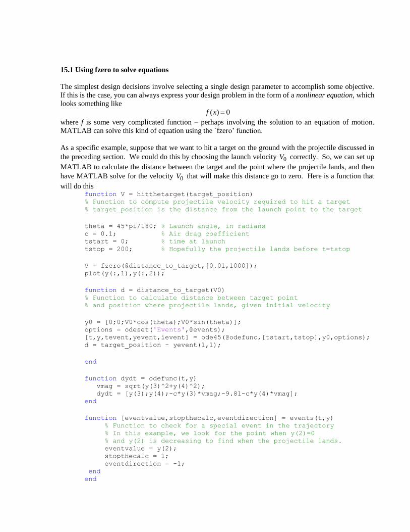
15.1 Using fzero to solve equations

The simplest design decisions involve selecting a single design parameter to accomplish some objective.

If this is the case, you can always express your design problem in the form of a nonlinear equation, which

looks something like

( ) 0f x

where f is some very complicated function – perhaps involving the solution to an equation of motion.

MATLAB can solve this kind of equation using the `fzero‟ function.

As a specific example, suppose that we want to hit a target on the ground with the projectile discussed in

the preceding section. We could do this by choosing the launch velocity 0V correctly. So, we can set up

MATLAB to calculate the distance between the target and the point where the projectile lands, and then

have MATLAB solve for the velocity 0V that will make this distance go to zero. Here is a function that

will do this function V = hitthetarget(target_position) % Function to compute projectile velocity required to hit a target % target_position is the distance from the launch point to the target

theta = 45*pi/180; % Launch angle, in radians c = 0.1; % Air drag coefficient tstart = 0; % time at launch tstop = 200; % Hopefully the projectile lands before t=tstop

V = fzero(@distance_to_target,[0.01,1000]); plot(y(:,1),y(:,2));

function d = distance_to_target(V0) % Function to calculate distance between target point % and position where projectile lands, given initial velocity

y0 = [0;0;V0*cos(theta);V0*sin(theta)]; options = odeset('Events',@events); [t,y,tevent,yevent,ievent] = ode45(@odefunc,[tstart,tstop],y0,options); d = target_position - yevent(1,1);

end

function dydt = odefunc(t,y) vmag = sqrt(y(3)^2+y(4)^2); dydt = [y(3);y(4);-c*y(3)*vmag;-9.81-c*y(4)*vmag]; end

function [eventvalue,stopthecalc,eventdirection] = events(t,y) % Function to check for a special event in the trajectory % In this example, we look for the point when y(2)=0 % and y(2) is decreasing to find when the projectile lands. eventvalue = y(2); stopthecalc = 1; eventdirection = -1; end end

You can try running this with

>> hitthetarget(10)

The function will return the velocity required to hit the target.

Here‟s a brief explanation of how the function works.

Start by looking at the nested function called distance to target(V0). This function uses the

methods described in Section 14 to find the point where the projectile hits the ground – the

`events‟ function is used to detect the point, and the horizontal distance of the projectile at the

point where it hits the ground is extracted from the „yevent‟ variable. Then, the function

calculates the distance d between the target and this point.

The function „fzero(@function,[initial guess 1,initial guess 2])‟ then calculates the velocity that

makes d zero. The two guesses for the velocity must be chosen so that d<0 for one of the

guesses, and d>0 for the other. MATLAB will find a solution between these two points. In

general, it is usually best to plot the function to see what to use for the initial guess, but for this

particular example we know that if we make the velocity very small, we will undershoot the

target, and if we make it huge, we will overshoot, so we can just enter a small and a large

number for the initial guesses and hope for the best. If both guesses overshoot, or both

undershoot the target, MATLAB will terminate with an error message (try this for yourself)

15.2 Simple unconstrained optimization example

MATLAB has a very powerful suite of algorithms for numerical optimization. The simplest optimizer is

a function called „fminsearch,‟ which will look for the minimum of a function of several (unconstrained)

variables. As an example, we will show how to use this function to solve the projectile problem

discussed in the preceding section. This time, we hit the target by searching for values of the launch

angle and launch speed 0V that will minimize the distance to the target. Here‟s a script that will do

this function [V,theta] = hitthetarget(target_position) % Function to compute projectile velocity required to hit a target % target_position is the distance from the launch point to the target

c = 0.1; % Air drag coefficient tstart = 0; % time at launch tstop = 200; % Hopefully the projectile lands before t=tstop

[V,theta] = fminsearch(@distance_to_target,[10,pi*45/180]); plot(y(:,1),y(:,2));

function d = distance_to_target(params) % Function to calculate distance between target point % and position where projectile lands, given initial velocity

V0=params(1); theta = params(2); y0 = [0;0;V0*cos(theta);V0*sin(theta)]; options = odeset('Events',@events); [t,y,tevent,yevent,ievent] = ode45(@odefunc,[tstart,tstop],y0,options); d = abs(target_position - yevent(1,1));

end


function [eventvalue,stopthecalc,eventdirection] = events(t,y) % Function to check for a special event in the trajectory % In this example, we look % (1) for the point when y(2)=0 and y(2) is decreasing. % (2) for the point where y(4)=0 (the top of the bounce) eventvalue = y(2); stopthecalc = 1; eventdirection = -1; end end

You can try running this with

>> hitthetarget(10)

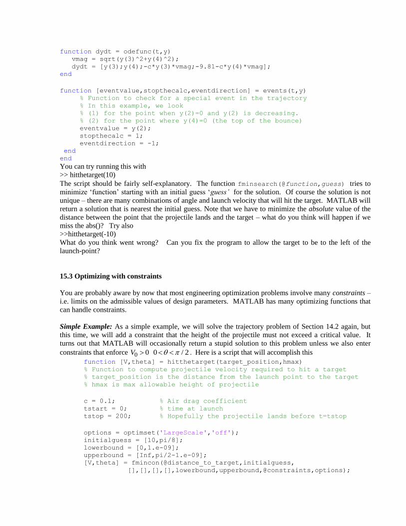
The script should be fairly self-explanatory. The function fminsearch(@function,guess) tries to

minimize „function‟ starting with an initial guess „guess’ for the solution. Of course the solution is not

unique – there are many combinations of angle and launch velocity that will hit the target. MATLAB will

return a solution that is nearest the initial guess. Note that we have to minimize the absolute value of the

distance between the point that the projectile lands and the target – what do you think will happen if we

miss the abs()? Try also

>>hitthetarget(-10)

What do you think went wrong? Can you fix the program to allow the target to be to the left of the

launch-point?

15.3 Optimizing with constraints

You are probably aware by now that most engineering optimization problems involve many constraints –

i.e. limits on the admissible values of design parameters. MATLAB has many optimizing functions that

can handle constraints.

Simple Example: As a simple example, we will solve the trajectory problem of Section 14.2 again, but

this time, we will add a constraint that the height of the projectile must not exceed a critical value. It

turns out that MATLAB will occasionally return a stupid solution to this problem unless we also enter

constraints that enforce 0 0V 0 / 2 . Here is a script that will accomplish this

function [V,theta] = hitthetarget(target_position,hmax) % Function to compute projectile velocity required to hit a target % target_position is the distance from the launch point to the target % hmax is max allowable height of projectile

c = 0.1; % Air drag coefficient tstart = 0; % time at launch tstop = 200; % Hopefully the projectile lands before t=tstop

options = optimset('LargeScale','off'); initialguess = [10,pi/8]; lowerbound = [0,1.e-09]; upperbound = [Inf,pi/2-1.e-09]; [V,theta] = fmincon(@distance_to_target,initialguess,

[],[],[],[],lowerbound,upperbound,@constraints,options);

plot(y(:,1),y(:,2));

function d = distance_to_target(variables) % Function to calculate distance between target point % and position where projectile lands, given initial velocity

V0 = variables(1); theta = variables(2); y0 = [0;0;V0*cos(theta);V0*sin(theta)]; options = odeset('Events',@events); [t,y,tevent,yevent,ievent] = ode45(@odefunc,[tstart,tstop],y0,options); d = abs(target_position - yevent(2,1)); % Bounce is always be 2nd event

end

function [c,ceq] = constraints(variables) % Function to impose constraints for nonlinear optimizer V0 = variables(1); theta = variables(2); y0 = [0;0;V0*cos(theta);V0*sin(theta)]; options = odeset('Events',@events); [t,y,tevent,yevent,ievent] =

ode45(@odefunc,[tstart,tstop],y0,options);

% This imposes the constraint that max value of y –hmax <= 0 c(1) = yevent(1,2)-hmax; % We know max height will be first event ceq = []; % There are no nonlinear equalities, so just return a

blank end


function [eventvalue,stopthecalc,eventdirection] = events(t,y) % Function to check for a special event in the trajectory % In this example, we look % (1) for the point when y(2)=0 and y(2) is decreasing. % (2) for the point where y(4)=0 (the top of the bounce) eventvalue = [y(2),y(4)]; stopthecalc = [1,0]; eventdirection = [-1,0];

end end

Try running this script first with

>> hitthetarget(10,10)

and then with

>> hitthetarget(10,1)

to check that it gives a solution that hits the target, and the max height is not exceeded. MATLAB will

return a rather incomprehensible message

Optimization terminated: magnitude of directional derivative in search

direction less than 2*options.TolFun and maximum constraint violation

is less than options.TolCon.

No active inequalities.

after you run the optimizer – just ignore this – it means everything worked.

Here‟s an explanation of how this script works. The constrained nonlinear optimizer is the function fmincon(@objective_function,initialguess,

A,b,Aeq,beq,lowerbound,upperbound,@constraints,options)

1. The „objective function’ specifies the function to be minimized. The solution calculated by the

function must always be a real number. It can be a function of as many (real valued) variables as

you like – the variables are specified as a vector that we will call x. In our example, the vector is

0[ , ]V

2. The „initial guess’ is a vector, which must provide an initial estimate for the solution x. If

possible, the initial guess should satisfy any constraints (exactly as for the EXCEL optimization

problems you solved last semester).

3. The arguments „A’ and „b’ are used to specify any constraints that have the form Ax b , where

A is a matrix, and b is a vector. There are no constraints like this in our example, so we just put

in a blank matrix and a blank vector.

4. The arguments Aeq and Beq enforce constraints of the form Ax b . Again, these are left blank

in our example.

5. The lowerbound and upperbound variables enforce constraints of the form min max x x x ,

where lowerbound is the lowest admissible value for the solution, and upperbound is the highest

admissible value for the solution. In our example, we enforce 00 V 9 910 / 2 10 .

6. The „constraints’ function is used to specify any constraints that can‟t be expressed in the forms

listed in 3-5. This function must always have the form

function [c,ceq] = function_name(variables)

where c is a vector, which can depend in some very complicated way on the variables, and „ceq‟

is another vector. MATLAB will attempt to find a solution satisfying 0c and ceq=0. In our

example, we only have one nonlinear constraint, and we simply set max max[ ] 0y h c . There

are no equations of the form ceq=0 in our example so we simply leave this part blank.

7. Finally the „options‟ variable is used to set various options – such as tolerances – for the

optimizer. In our example, we set the variable „largescale‟ to value „off‟ – this stops MATLAB

trying to use some heavy matrix machinery designed for problems with large numbers of

variables. If you omit this option MATLAB will just give you a warning that these methods don‟t

work for this problem, and continue without them.

Complex example: For a more difficult problem, the script below solves the Ferryboat optimization

problem set as a problem last year in EN30 (see

http://www.engin.brown.edu/courses/en3/Homeworks/2008/hw2/hw2.pdf for a full statement of the

problem). function sol = crosstheriver(W,d,Vboat,V0) % Function to solve the EN3 Ferryboat optimization problem % W is the width of the river, d is the distance traveled upstream, % Vboat is the ferry speed through the water, and V0 is the max % speed of the river. The function finds the path that % minimizes the crossing time. % n_segments = 50; % segments in the path options = optimset('LargeScale','off'); % The variables are [theta_i,s] where theta_i are the angles of each

% path segment, and s is the length of the segments.

% For the initial guess we use a straight path across the river.

% This works as long as the river speed is not too large

http://www.engin.brown.edu/courses/en3/Homeworks/2008/hw2/hw2.pdf

% - for large values of river speed you would have to use a different % initial guess. initialguess(1:n_segments) = atan(W/d); initialguess(n_segments+1) = sqrt(W^2+d^2)/n_segments;

sol =

fmincon(@timetocross,initialguess,[],[],[],[],[],[],@constraints,option

s); plot([0,x],[0,y]); % Plots the path – (0,0) is included as a point.

function t = timetocross(variables) % Function to calculate the time taken by % the boat to cross the river, given % angles of path segments and segment length

theta(1:n_segments) = variables(1:n_segments); s = variables(n_segments+1); % Calculate end point of each segment and height % of mid-point of each segment x(1) = s*cos(theta(1)); y(1) = s*sin(theta(1)); ybar(1) = y(1)/2; for i=2:n_segments x(i)=x(i-1)+s*cos(theta(i)); %x-coord of end point y(i)=y(i-1)+s*sin(theta(i)); %y coord of end point ybar(i) = (y(i-1)+y(i))/2; % y coord of mid point end % Now calculate the crossing time t = 0; for i=1:n_segments Vr = 4*W*ybar(i)*V0*(W-ybar(i))/W^2; %River speed V = sqrt(Vboat^2-Vr^2*sin(theta(i))^2)-Vr*cos(theta(i)); %Ferry

speed t = t + s/V; % Add time to travel ith segment to total end

end

function [c,ceq] = constraints(variables) % Function to enforce constraints

theta(1:n_segments) = variables(1:n_segments); s = variables(n_segments+1); x(1) = s*cos(theta(1)); y(1) = s*sin(theta(1)); for i=2:n_segments x(i)=x(i-1)+s*cos(theta(i)); y(i)=y(i-1)+s*sin(theta(i)); end c = -y; % This prevents y<0 for all points on the path c=[c,y-W]; % This prevents y>W for all points on the path ceq = [W-y(n_segments),d-x(n_segments)]; % This enforces y=W,x=d at end

of path end

end

Try running the script with

>> crosstheriver(1,2,15,10)

MATLAB should plot the optimal path for you, as shown below

You should notice that MATLAB runs far faster than EXCEL, even though this example uses a large

number of points on the path, and has many more constraints than you used in the EXCEL example.

For further details about MATLAB optimization, you can consult the manual in the section listed below.

16. Reading and writing data to/from files

MATLAB is often used to process experimental data, or to prepare data that will be used in another

program. For this purpose, you will need to read and write data from files. Learning to read and write

data is perhaps the most difficult part of learning MATLAB, and is usually a big headache in mastering

any new programming language. Don‟t worry if this section looks scary – you won‟t need to do any

complicated file I/O in this class. You could even skip this section altogether the first time you do this

tutorial, and come back to it later.

MATLAB can read a large number of different types of file, including simple text files, excel worksheets,

word documents, pdf files, and even audio and video files. We will only look at a small subset of these

here.

Comma separated value files are the simplest way to get numerical data in and out of MATLAB. For

example, try the following in the command window

>> A = pascal(5);

>> csvwrite(„examplefile1.dat‟,A);

Then open the file examplefile1.dat with a text editor (Notepad will do). You should find that the file

contains a bunch of numbers separated by commas. Each row of the matrix appears on a separate line.

You can read the file back into MATLAB using

>> B = csvread(„examplefile1.dat);

>> B

If you are using this method to read experimental data, and need to know how much data is in the file, the

command

>>[nrows,ncols]=size(B)

will tell you how many rows and columns of data were read from the file.

Using the ‘import’ wizard Simple files, such as comma-separated-value files, simple spreadsheets, audio

files, etc can often be read using the „import‟ wizard. To try this, right-click the „examplefile1.dat‟ file in

the directory window (see below)

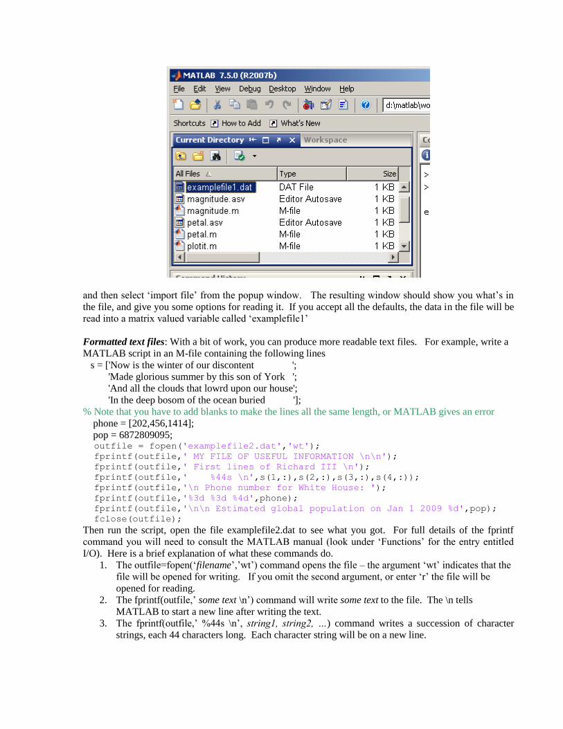
and then select „import file‟ from the popup window. The resulting window should show you what‟s in

the file, and give you some options for reading it. If you accept all the defaults, the data in the file will be

read into a matrix valued variable called „examplefile1‟

Formatted text files: With a bit of work, you can produce more readable text files. For example, write a

MATLAB script in an M-file containing the following lines

s = ['Now is the winter of our discontent ';

'Made glorious summer by this son of York ';

'And all the clouds that lowrd upon our house';

'In the deep bosom of the ocean buried '];

% Note that you have to add blanks to make the lines all the same length, or MATLAB gives an error

phone = [202,456,1414];

pop = 6872809095; outfile = fopen('examplefile2.dat','wt'); fprintf(outfile,' MY FILE OF USEFUL INFORMATION \n\n'); fprintf(outfile,' First lines of Richard III \n'); fprintf(outfile,' %44s \n',s(1,:),s(2,:),s(3,:),s(4,:)); fprintf(outfile,'\n Phone number for White House: '); fprintf(outfile,'%3d %3d %4d',phone); fprintf(outfile,'\n\n Estimated global population on Jan 1 2009 %d',pop); fclose(outfile);

Then run the script, open the file examplefile2.dat to see what you got. For full details of the fprintf

command you will need to consult the MATLAB manual (look under „Functions‟ for the entry entitled

I/O). Here is a brief explanation of what these commands do.

1. The outfile=fopen(„filename‟,‟wt‟) command opens the file – the argument „wt‟ indicates that the

file will be opened for writing. If you omit the second argument, or enter „r‟ the file will be

opened for reading.

2. The fprintf(outfile,‟ some text \n‟) command will write some text to the file. The \n tells

MATLAB to start a new line after writing the text.

3. The fprintf(outfile,‟ %44s \n‟, string1, string2, …) command writes a succession of character

strings, each 44 characters long. Each character string will be on a new line.

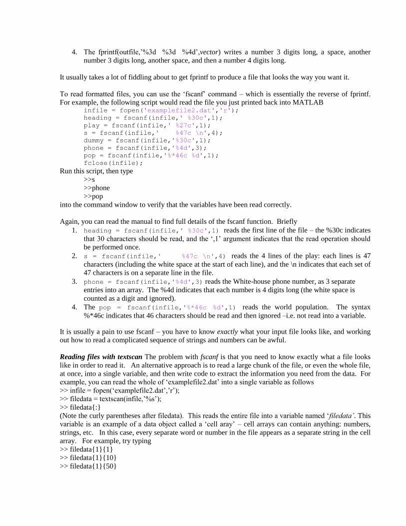
4. The fprintf(outfile,‟%3d %3d %4d‟,vector) writes a number 3 digits long, a space, another

number 3 digits long, another space, and then a number 4 digits long.

It usually takes a lot of fiddling about to get fprintf to produce a file that looks the way you want it.

To read formatted files, you can use the „fscanf‟ command – which is essentially the reverse of fprintf.

For example, the following script would read the file you just printed back into MATLAB infile = fopen('examplefile2.dat','r'); heading = fscanf(infile,' %30c',1); play = fscanf(infile,' %27c',1); s = fscanf(infile,' %47c \n',4); dummy = fscanf(infile,'%30c',1); phone = fscanf(infile,'%4d',3); pop = fscanf(infile,'%*46c %d',1); fclose(infile);

Run this script, then type

>>s

>>phone

>>pop

into the command window to verify that the variables have been read correctly.

Again, you can read the manual to find full details of the fscanf function. Briefly

1. heading = fscanf(infile,' %30c',1) reads the first line of the file – the %30c indicates

that 30 characters should be read, and the „,1‟ argument indicates that the read operation should

be performed once.

2. s = fscanf(infile,' %47c \n',4) reads the 4 lines of the play: each lines is 47

characters (including the white space at the start of each line), and the \n indicates that each set of

47 characters is on a separate line in the file.

3. phone = fscanf(infile,'%4d',3) reads the White-house phone number, as 3 separate

entries into an array. The %4d indicates that each number is 4 digits long (the white space is

counted as a digit and ignored).

4. The pop = fscanf(infile,'%*46c %d',1) reads the world population. The syntax

%*46c indicates that 46 characters should be read and then ignored –i.e. not read into a variable.

It is usually a pain to use fscanf – you have to know exactly what your input file looks like, and working

out how to read a complicated sequence of strings and numbers can be awful.

Reading files with textscan The problem with fscanf is that you need to know exactly what a file looks

like in order to read it. An alternative approach is to read a large chunk of the file, or even the whole file,

at once, into a single variable, and then write code to extract the information you need from the data. For

example, you can read the whole of „examplefile2.dat‟ into a single variable as follows

>> infile = fopen(„examplefile2.dat‟,‟r‟);

>> filedata = textscan(infile,‟%s‟);

>> filedata{:}

(Note the curly parentheses after filedata). This reads the entire file into a variable named „filedata’. This

variable is an example of a data object called a „cell aray‟ – cell arrays can contain anything: numbers,

strings, etc. In this case, every separate word or number in the file appears as a separate string in the cell

array. For example, try typing

>> filedata{1}{1}

>> filedata{1}{10}

>> filedata{1}{50}

This will display the first, 10th and 50

th distinct word in the file. Another way to display the entire

contents of a cell array is

>>celldisp(filedata)

You can now extract the bits of the file that you are interested in into separate variables. For example, try

>> pop = str2num(filedata{1}{58});

>> for n=1:3 phone(n) = str2num(filedata{1},{47+n}); end

>> pop

>> phone

Here, the „str2num‟ function converts a string of characters into a number. (The distinction between a

string of numerical characters and a number is apparent only to computers, not to humans. But the

computers are in charge and we have to humor them).

Challenge: see if you can reconstruct the variable „s‟ containing the Shakespeare. This is quite tricky…

MATLAB can read many other types of file. If you are using a Windows PC, and enjoy bagpipe music,

you could download this file and then type

>> [y,fs,n] = wavread(filename);

>> wavplay(y,fs);

17. Animations

In dynamics problems it is often fun to generate a movie or animation that illustrates the motion of the

system you are trying to model. The animations don‟t always tell you anything useful, but they are

useful to kill time in a boring presentation or to impress senior management.

Making movies in MATLAB is simple – you just need to generate a sequence of plots, save them, and

then play them back as a movie. But animations can be a bit of a chore – it can take some fiddling about

to get MATLAB to plot frames at equal time intervals, and it is tedious to draw complicated shapes –

everything needs to be built from scratch by drawing 2D or 3D polygons.

As always, the procedure is best illustrated with examples.

Example 1: Movie of a flying projectile: The script below makes a movie showing the path of a projectile function M = trajectorymovie(V0,theta,c,n_frames) % Function to make a movie of the trajectory of a projectile

theta = theta*pi/180; % convert theta to radians y0 = [0;0;V0*cos(theta);V0*sin(theta)];

options = odeset('Events',@events); sol = ode45(@odefunc,[0,Inf],y0,options);

% All this bookkeeping is simply to % scale the axes so the projectile does % not leave the frame. tpeak = sol.xe(1); %Get the time at max height ymax = deval(sol,tpeak,[2]); % Get max height tbounce = sol.xe(2); %Get the time at bouncing xmax = deval(sol,tbounce,[1]); % Get distance traveled axis_length = max([xmax,ymax]);

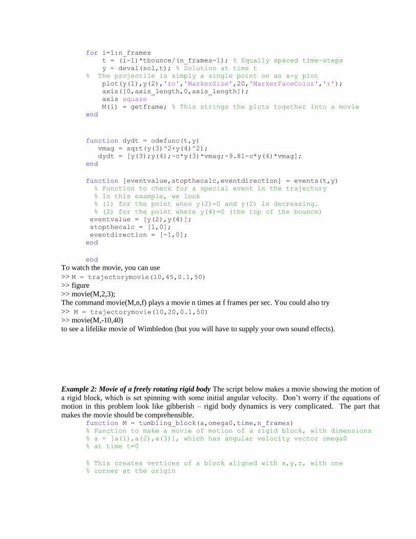
for i=1:n_frames

t = (i-1)*tbounce/(n_frames-1); % Equally spaced time-steps y = deval(sol,t); % Solution at time t % The projectile is simply a single point on an x-y plot plot(y(1),y(2),'ro','MarkerSize',20,'MarkerFaceColor','r'); axis([0,axis_length,0,axis_length]); axis square M(i) = getframe; % This strings the plots together into a movie end


function [eventvalue,stopthecalc,eventdirection] = events(t,y) % Function to check for a special event in the trajectory % In this example, we look % (1) for the point when y(2)=0 and y(2) is decreasing. % (2) for the point where y(4)=0 (the top of the bounce) eventvalue = [y(2),y(4)]; stopthecalc = [1,0]; eventdirection = [-1,0]; end

end

To watch the movie, you can use

>> M = trajectorymovie(10,45,0.1,50)

>> figure

>> movie(M,2,3);

The command movie(M,n,f) plays a movie n times at f frames per sec. You could also try

>> M = trajectorymovie(10,20,0.1,50)

>> movie(M,-10,40)

to see a lifelike movie of Wimbledon (but you will have to supply your own sound effects).

Example 2: Movie of a freely rotating rigid body The script below makes a movie showing the motion of

a rigid block, which is set spinning with some initial angular velocity. Don‟t worry if the equations of

motion in this problem look like gibberish – rigid body dynamics is very complicated. The part that

makes the movie should be comprehensible. function M = tumbling_block(a,omega0,time,n_frames) % Function to make a movie of motion of a rigid block, with dimensions % a = [a(1),a(2),a(3)], which has angular velocity vector omega0 % at time t=0

% This creates vertices of a block aligned with x,y,z, with one

% corner at the origin

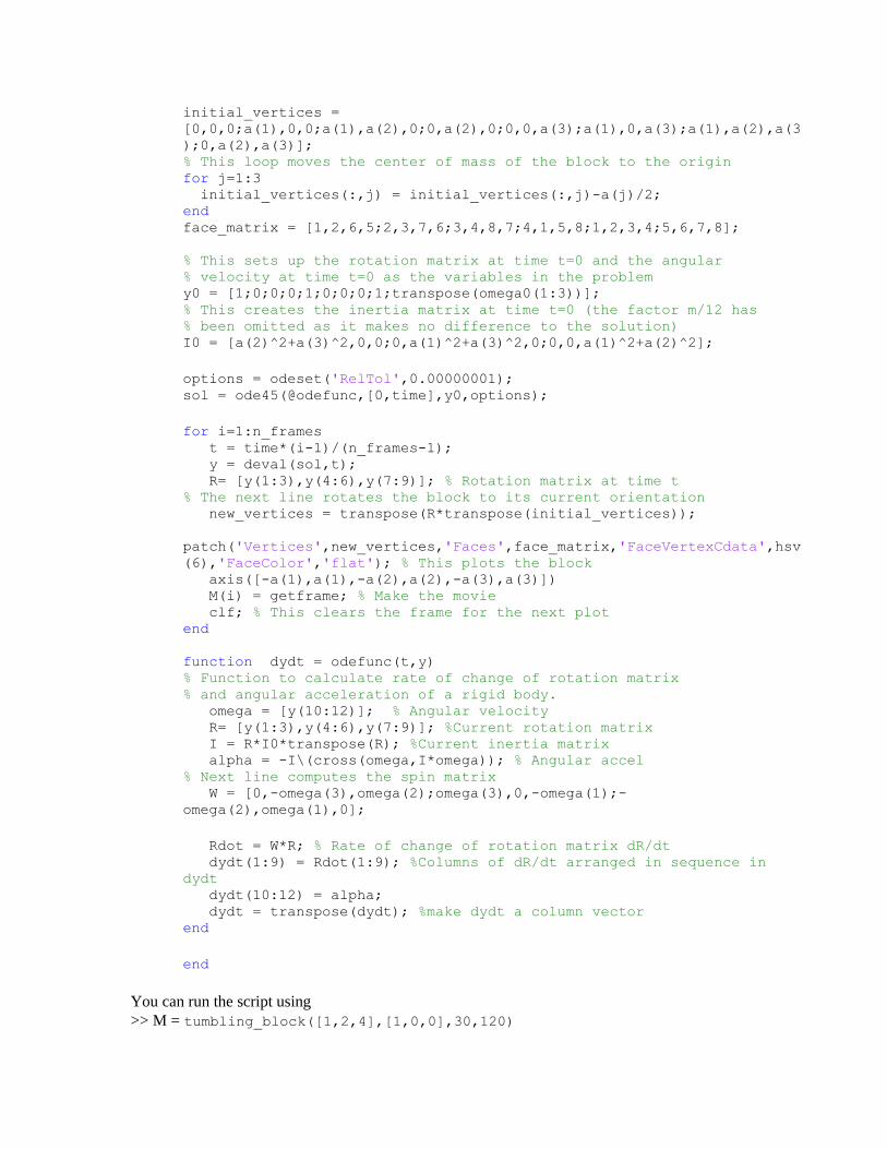
initial_vertices =

[0,0,0;a(1),0,0;a(1),a(2),0;0,a(2),0;0,0,a(3);a(1),0,a(3);a(1),a(2),a(3

);0,a(2),a(3)];

% This loop moves the center of mass of the block to the origin for j=1:3 initial_vertices(:,j) = initial_vertices(:,j)-a(j)/2; end face_matrix = [1,2,6,5;2,3,7,6;3,4,8,7;4,1,5,8;1,2,3,4;5,6,7,8];

% This sets up the rotation matrix at time t=0 and the angular

% velocity at time t=0 as the variables in the problem

y0 = [1;0;0;0;1;0;0;0;1;transpose(omega0(1:3))];

% This creates the inertia matrix at time t=0 (the factor m/12 has

% been omitted as it makes no difference to the solution) I0 = [a(2)^2+a(3)^2,0,0;0,a(1)^2+a(3)^2,0;0,0,a(1)^2+a(2)^2];

options = odeset('RelTol',0.00000001); sol = ode45(@odefunc,[0,time],y0,options);

for i=1:n_frames t = time*(i-1)/(n_frames-1); y = deval(sol,t); R= [y(1:3),y(4:6),y(7:9)]; % Rotation matrix at time t

% The next line rotates the block to its current orientation new_vertices = transpose(R*transpose(initial_vertices));

patch('Vertices',new_vertices,'Faces',face_matrix,'FaceVertexCdata',hsv

(6),'FaceColor','flat'); % This plots the block axis([-a(1),a(1),-a(2),a(2),-a(3),a(3)]) M(i) = getframe; % Make the movie

clf; % This clears the frame for the next plot end

function dydt = odefunc(t,y) % Function to calculate rate of change of rotation matrix

% and angular acceleration of a rigid body.

omega = [y(10:12)]; % Angular velocity R= [y(1:3),y(4:6),y(7:9)]; %Current rotation matrix I = R*I0*transpose(R); %Current inertia matrix

alpha = -I\(cross(omega,I*omega)); % Angular accel

% Next line computes the spin matrix W = [0,-omega(3),omega(2);omega(3),0,-omega(1);-

omega(2),omega(1),0];

Rdot = W*R; % Rate of change of rotation matrix dR/dt dydt(1:9) = Rdot(1:9); %Columns of dR/dt arranged in sequence in

dydt dydt(10:12) = alpha; dydt = transpose(dydt); %make dydt a column vector end

end

You can run the script using

>> M = tumbling_block([1,2,4],[1,0,0],30,120)

This will start the block spinning about the x – axis. To watch the movie, you can use

>> movie(M,1,20)

The „patch‟ function draws a 3D polygonal shape – you have to tell it the coordinates of each vertex on

the polygon (stored in the „new_vertices,‟ matrix) and you also need to specify how the vertices are

arranged on each face of the block (each row of the `face matrix‟ lists the vertices on one face of the

block). Type

>> help patch

in the command window for more details of how this function works.

This simulation can demonstrate the complicated behavior of spinning objects. Try spinning the block

about the z axis, by using

>> M = tumbling_block([1,2,4],[0,0,1],30,120)

You should see that the block simply keeps rotating about the z axis. You can show that, for this

particular block, rotation about the x and z axes is stable – for example, try

>> M = tumbling_block([1,2,4],[0,0.001,1],30,120)

This spins the block about an axis that is very nearly parallel to the z axis but not quite. You won‟t see

any change in the motion of the block – it will simply look as though it is rotating about the z axis.

However, if you try the same test by starting the block spinning about an axis very near the y direction

>> M = tumbling_block([1,2,4],[0.0,1,0.001],30,120)

you will see the block do some strange flips mid-rotation. This is not a simulation error – it is real

behavior. You can verify the prediction experimentally by flipping a book.

18. On the frustrations of scientific programming

Hopefully you have been able to execute the scripts and examples in this tutorial without any problems.

When you start writing your own scripts and functions, however, you will almost certainly find that they

don‟t work. You will find this absolutely maddening – the tutorial makes everything look easy – so why

don‟t your programs work?

Don‟t get discouraged – this is totally normal. If it is any consolation, I screwed up every single script in

this tutorial when I first wrote them – even the little short trivial ones that are only a few lines long. This

sort of thing no longer fazes me – for planning purposes I always assume it will take me longer to fix the

errors in my programs than it did to design and code them, and over the years I have learned how to find

and fix errors fairly quickly.

My programming errors are one of the following:

1. Stupid typos and mistakes – these are annoying, but can usually be found quickly. If MATLAB

finds a typo it usually tells you which line is causing problems (the M-file editor also gives

warnings about potential problems). The typos and mistakes that are hardest find are the ones

that send the program into an infinite loop, or weird memory management problems that cause

variables to be assigned incorrect values (eg by setting pi=3). To find these, you need to identify

where they occur in the code – you can use a debugger for this, or if you prefer you can simply

have your program print messages as it completes bits of your calculation, so you know where it

hangs up.

2. I did not read the manual carefully enough – the MATLAB function I am trying to use doesn‟t

do what I think it does, I have forgotten some variables that are needed for the function, etc.

Again, these errors aren‟t hard to find as long as I am not too lazy to read the manual. If I can‟t

get a MATLAB function to work I will often try using it to solve a much simpler problem as a

test case.

3. There is a fundamental flaw in the algorithm that I am trying to use. As a student I once wrote

an optimization program several thousand lines long, which would always return the initial guess

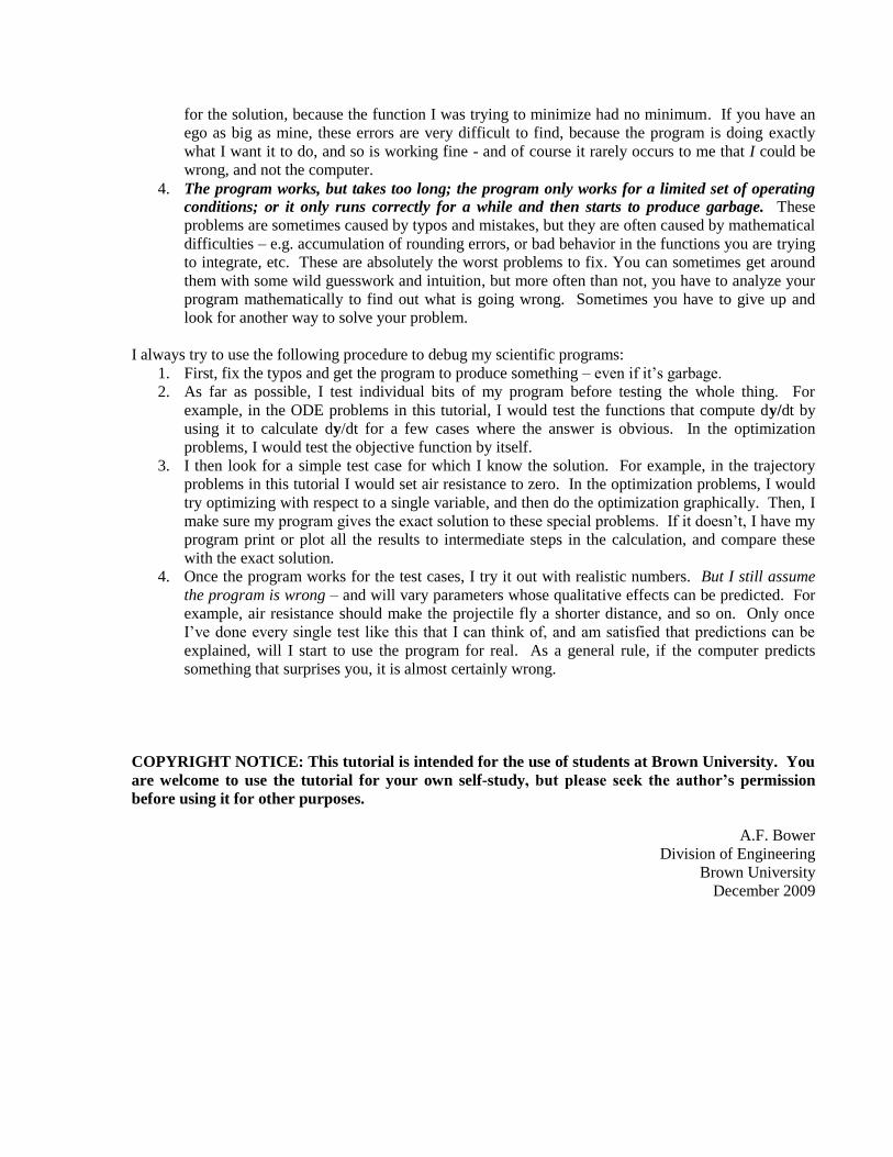
for the solution, because the function I was trying to minimize had no minimum. If you have an

ego as big as mine, these errors are very difficult to find, because the program is doing exactly

what I want it to do, and so is working fine - and of course it rarely occurs to me that I could be

wrong, and not the computer.

4. The program works, but takes too long; the program only works for a limited set of operating

conditions; or it only runs correctly for a while and then starts to produce garbage. These

problems are sometimes caused by typos and mistakes, but they are often caused by mathematical

difficulties – e.g. accumulation of rounding errors, or bad behavior in the functions you are trying

to integrate, etc. These are absolutely the worst problems to fix. You can sometimes get around

them with some wild guesswork and intuition, but more often than not, you have to analyze your

program mathematically to find out what is going wrong. Sometimes you have to give up and

look for another way to solve your problem.

I always try to use the following procedure to debug my scientific programs:

1. First, fix the typos and get the program to produce something – even if it‟s garbage.

2. As far as possible, I test individual bits of my program before testing the whole thing. For

example, in the ODE problems in this tutorial, I would test the functions that compute dy/dt by

using it to calculate dy/dt for a few cases where the answer is obvious. In the optimization

problems, I would test the objective function by itself.

3. I then look for a simple test case for which I know the solution. For example, in the trajectory

problems in this tutorial I would set air resistance to zero. In the optimization problems, I would

try optimizing with respect to a single variable, and then do the optimization graphically. Then, I

make sure my program gives the exact solution to these special problems. If it doesn‟t, I have my

program print or plot all the results to intermediate steps in the calculation, and compare these

with the exact solution.

4. Once the program works for the test cases, I try it out with realistic numbers. But I still assume

the program is wrong – and will vary parameters whose qualitative effects can be predicted. For

example, air resistance should make the projectile fly a shorter distance, and so on. Only once

I‟ve done every single test like this that I can think of, and am satisfied that predictions can be

explained, will I start to use the program for real. As a general rule, if the computer predicts

something that surprises you, it is almost certainly wrong.

COPYRIGHT NOTICE: This tutorial is intended for the use of students at Brown University. You

are welcome to use the tutorial for your own self-study, but please seek the author’s permission

before using it for other purposes.

A.F. Bower

Division of Engineering

Brown University

December 2009

MATLAB Tutorial

Documents

Transcript of MATLAB Tutorial