Matlab Signal Processing
418
-
Upload
nguyen-kien-long -
Category
Documents
-
view
11.220 -
download
46
Transcript of Matlab Signal Processing
JWBK207-FM JWBK207-Shin February 1, 2008 21:27 Char Count= 0
Fundamentals of Signal
Processingfor Sound and Vibration Engineers
Kihong ShinAndong National University
Republic of Korea
Joseph K. HammondUniversity of Southampton
UK
John Wiley & Sons, Ltd
iii

JWBK207-FM JWBK207-Shin February 1, 2008 21:27 Char Count= 0
ii
JWBK207-FM JWBK207-Shin February 1, 2008 21:27 Char Count= 0
Fundamentals of Signal Processing
for Sound and Vibration Engineers
i

JWBK207-FM JWBK207-Shin February 1, 2008 21:27 Char Count= 0
ii

JWBK207-FM JWBK207-Shin February 1, 2008 21:27 Char Count= 0
Fundamentals of Signal
Processingfor Sound and Vibration Engineers
Kihong ShinAndong National University
Republic of Korea
Joseph K. HammondUniversity of Southampton
UK
John Wiley & Sons, Ltd
iii

JWBK207-FM JWBK207-Shin February 1, 2008 21:27 Char Count= 0
Copyright C© 2008 John Wiley & Sons Ltd, The Atrium, Southern Gate, Chichester,West Sussex PO19 8SQ, England
Telephone (+44) 1243 779777
Email (for orders and customer service enquiries): [email protected] our Home Page on www.wileyeurope.com or www.wiley.com
All Rights Reserved. No part of this publication may be reproduced, stored in a retrieval system or transmitted inany form or by any means, electronic, mechanical, photocopying, recording, scanning or otherwise, except underthe terms of the Copyright, Designs and Patents Act 1988 or under the terms of a licence issued by the CopyrightLicensing Agency Ltd, 90 Tottenham Court Road, London W1T 4LP, UK, without the permission in writing of thePublisher. Requests to the Publisher should be addressed to the Permissions Department, John Wiley & Sons Ltd,The Atrium, Southern Gate, Chichester, West Sussex PO19 8SQ, England, or emailed to [email protected], orfaxed to (+44) 1243 770620.
This publication is designed to provide accurate and authoritative information in regard to the subject mattercovered. It is sold on the understanding that the Publisher is not engaged in rendering professional services. Ifprofessional advice or other expert assistance is required, the services of a competent professional should be sought.
Other Wiley Editorial Offices
John Wiley & Sons Inc., 111 River Street, Hoboken, NJ 07030, USA
Jossey-Bass, 989 Market Street, San Francisco, CA 94103-1741, USA
Wiley-VCH Verlag GmbH, Boschstr. 12, D-69469 Weinheim, Germany
John Wiley & Sons Australia Ltd, 42 McDougall Street, Milton, Queensland 4064, Australia
John Wiley & Sons (Asia) Pte Ltd, 2 Clementi Loop #02-01, Jin Xing Distripark, Singapore 129809
John Wiley & Sons Canada Ltd, 6045 Freemont Blvd, Mississauga, ONT, L5R 4J3
Wiley also publishes its books in a variety of electronic formats. Some content that appears in print maynot be available in electronic books.
Library of Congress Cataloging-in-Publication Data
Shin, Kihong.Fundamentals of signal processing for sound and vibration engineers / Kihong Shin and
Joseph Kenneth Hammond.p. cm.
Includes bibliographical references and index.ISBN 978-0-470-51188-6 (cloth)
1. Signal processing. 2. Acoustical engineering. 3. Vibration. I. Hammond, Joseph Kenneth.II. Title.
TK5102.9.S5327 2007621.382′2—dc22 2007044557
British Library Cataloguing in Publication Data
A catalogue record for this book is available from the British Library
ISBN-13 978-0470-51188-6
Typeset in 10/12pt Times by Aptara, New Delhi, India.Printed and bound in Great Britain by Antony Rowe Ltd, Chippenham, WiltshireThis book is printed on acid-free paper responsibly manufactured from sustainable forestry in which at least twotrees are planted for each one used for paper production.
MATLAB R© is a trademark of The MathWorks, Inc. and is used with permission. The MathWorks does not warrantthe accuracy of the text or exercises in this book. This book’s use or discussion of MATLAB R© software or relatedproducts does not constitute endorsement or sponsorship by The MathWorks of a particular pedagogical approachor particular use of the MATLAB R© software.
iv
JWBK207-FM JWBK207-Shin February 1, 2008 21:27 Char Count= 0
Contents
Preface ixAbout the Authors xi
1 Introduction to Signal Processing 11.1 Descriptions of Physical Data (Signals) 61.2 Classification of Data 7
Part I Deterministic Signals 17
2 Classification of Deterministic Data 192.1 Periodic Signals 192.2 Almost Periodic Signals 212.3 Transient Signals 242.4 Brief Summary and Concluding Remarks 242.5 MATLAB Examples 26
3 Fourier Series 313.1 Periodic Signals and Fourier Series 313.2 The Delta Function 383.3 Fourier Series and the Delta Function 413.4 The Complex Form of the Fourier Series 423.5 Spectra 433.6 Some Computational Considerations 463.7 Brief Summary 523.8 MATLAB Examples 52
4 Fourier Integrals (Fourier Transform) and Continuous-Time Linear Systems 574.1 The Fourier Integral 574.2 Energy Spectra 614.3 Some Examples of Fourier Transforms 624.4 Properties of Fourier Transforms 67
v

JWBK207-FM JWBK207-Shin February 1, 2008 21:27 Char Count= 0
vi CONTENTS
4.5 The Importance of Phase 714.6 Echoes 724.7 Continuous-Time Linear Time-Invariant Systems and Convolution 734.8 Group Delay (Dispersion) 824.9 Minimum and Non-Minimum Phase Systems 854.10 The Hilbert Transform 904.11 The Effect of Data Truncation (Windowing) 944.12 Brief Summary 1024.13 MATLAB Examples 103
5 Time Sampling and Aliasing 1195.1 The Fourier Transform of an Ideal Sampled Signal 1195.2 Aliasing and Anti-Aliasing Filters 1265.3 Analogue-to-Digital Conversion and Dynamic Range 1315.4 Some Other Considerations in Signal Acquisition 1345.5 Shannon’s Sampling Theorem (Signal Reconstruction) 1375.6 Brief Summary 1395.7 MATLAB Examples 140
6 The Discrete Fourier Transform 1456.1 Sequences and Linear Filters 1456.2 Frequency Domain Representation of Discrete Systems and Signals 1506.3 The Discrete Fourier Transform 1536.4 Properties of the DFT 1606.5 Convolution of Periodic Sequences 1626.6 The Fast Fourier Transform 1646.7 Brief Summary 1666.8 MATLAB Examples 170
Part II Introduction to Random Processes 191
7 Random Processes 1937.1 Basic Probability Theory 1937.2 Random Variables and Probability Distributions 1987.3 Expectations of Functions of a Random Variable 2027.4 Brief Summary 2117.5 MATLAB Examples 212
8 Stochastic Processes; Correlation Functions and Spectra 2198.1 Probability Distribution Associated with a Stochastic Process 2208.2 Moments of a Stochastic Process 2228.3 Stationarity 2248.4 The Second Moments of a Stochastic Process; Covariance
(Correlation) Functions 2258.5 Ergodicity and Time Averages 2298.6 Examples 232
JWBK207-FM JWBK207-Shin February 1, 2008 21:27 Char Count= 0
CONTENTS vii
8.7 Spectra 2428.8 Brief Summary 2518.9 MATLAB Examples 253
9 Linear System Response to Random Inputs: System Identification 2779.1 Single-Input Single-Output Systems 2779.2 The Ordinary Coherence Function 2849.3 System Identification 2879.4 Brief Summary 2979.5 MATLAB Examples 298
10 Estimation Methods and Statistical Considerations 31710.1 Estimator Errors and Accuracy 31710.2 Mean Value and Mean Square Value 32010.3 Correlation and Covariance Functions 32310.4 Power Spectral Density Function 32710.5 Cross-spectral Density Function 34710.6 Coherence Function 34910.7 Frequency Response Function 35010.8 Brief Summary 35210.9 MATLAB Examples 354
11 Multiple-Input/Response Systems 36311.1 Description of Multiple-Input, Multiple-Output (MIMO) Systems 36311.2 Residual Random Variables, Partial and Multiple Coherence Functions 36411.3 Principal Component Analysis 370
Appendix A Proof of∫ ∞
−∞2M sin 2πaM2πaM
da = 1 375
Appendix B Proof of |Sxy( f )|2 ≤ Sxx( f )Syy( f ) 379
Appendix C Wave Number Spectra and an Application 381
Appendix D Some Comments on the Ordinary CoherenceFunction γ2
xy( f ) 385
Appendix E Least Squares Optimization: Complex-Valued Problem 387
Appendix F Proof of HW ( f ) → H1( f ) as κ( f ) → ∞ 389
Appendix G Justification of the Joint Gaussianity of X( f ) 391
Appendix H Some Comments on Digital Filtering 393
References 395
Index 399

JWBK207-FM JWBK207-Shin February 1, 2008 21:27 Char Count= 0
viii
JWBK207-FM JWBK207-Shin February 1, 2008 21:27 Char Count= 0
Preface
This book has grown out of notes for a course that the second author has given for moreyears than he cares to remember – which, but for the first author who kept various versions,would never have come to this. Specifically, the Institute of Sound and Vibration Research(ISVR) at the University of Southampton has, for many years, run a Masters programmein Sound and Vibration, and more recently in Applied Digital Signal Processing. A courseaimed at introducing students to signal processing has been one of the compulsory mod-ules, and given the wide range of students’ first degrees, the coverage needs to make fewassumptions about prior knowledge – other than a familiarity with degree entry-level math-ematics. In addition to the Masters programmes the ISVR runs undergraduate programmesin Acoustical Engineering, Acoustics with Music, and Audiology, each of which to varyinglevels includes signal processing modules. These taught elements underpin the wide-rangingresearch of the ISVR, exemplified by the four interlinked research groups in Dynamics,Fluid Dynamics and Acoustics, Human Sciences, and Signal Processing and Control. Thelarge doctoral cohort in the research groups attend selected Masters modules and an acquain-tance with signal processing is a ‘required skill’ (necessary evil?) in many a research project.Building on the introductory course there are a large number of specialist modules rangingfrom medical signal processing to sonar, and from adaptive and active control to Bayesianmethods.
It was in one of the PhD cohorts that Kihong Shin and Joe Hammond made each other’sacquaintance in 1994. Kihong Shin received his PhD from ISVR in 1996 and was then apostdoctoral research fellow with Professor Mike Brennan in the Dynamics Group, thenjoining the School of Mechanical Engineering, Andong National University, Korea, in 2002,where he is an associate professor. This marked the start of this book, when he began ‘editing’Joe Hammond’s notes appropriate to a postgraduate course he was lecturing – particularlyappreciating the importance of including ‘hands-on’ exercises – using interactive MATLAB R©
examples. With encouragement from Professor Mike Brennan, Kihong Shin continued withthis and it was not until 2004, when a manuscript landed on Joe Hammond’s desk (some bitslooking oddly familiar), that the second author even knew of the project – with some surpriseand great pleasure.
ix

JWBK207-FM JWBK207-Shin February 1, 2008 21:27 Char Count= 0
x PREFACE
In July 2006, with the kind support and consideration of Professor Mike Brennan, KihongShin managed to take a sabbatical which he spent at the ISVR where his subtle pressures –including attending Joe Hammond’s very last course on signal processing at the ISVR – havedistracted Joe Hammond away from his duties as Dean of the Faculty of Engineering, Scienceand Mathematics.
Thus the text was completed. It is indeed an introduction to the subject and therefore theessential material is not new and draws on many classic books. What we have tried to do isto bring material together, hopefully encouraging the reader to question, enquire about andexplore the concepts using the MATLAB exercises or derivatives of them.
It only remains to thank all who have contributed to this. First, of course, the authorswhose texts we have referred to, then the decades of students at the ISVR, and more recentlyin the School of Mechanical Engineering, Andong National University, who have shaped theway the course evolved, especially Sangho Pyo who spent a generous amount of time gath-ering experimental data. Two colleagues in the ISVR deserve particular gratitude: ProfessorMike Brennan, whose positive encouragement for the whole project has been essential, to-gether with his very constructive reading of the manuscript; and Professor Paul White, whoseencyclopaedic knowledge of signal processing has been our port of call when we neededreassurance.
We would also like to express special thanks to our families, Hae-Ree Lee, Inyong Shin,Hakdoo Yu, Kyu-Shin Lee, Young-Sun Koo and Jill Hammond, for their never-ending supportand understanding during the gestation and preparation of the manuscript. Kihong Shin is alsograteful to Geun-Tae Yim for his continuing encouragement at the ISVR.
Finally, Joe Hammond thanks Professor Simon Braun of the Technion, Haifa, for hisunceasing and inspirational leadership of signal processing in mechanical engineering. Also,and very importantly, we wish to draw attention to a new text written by Simon entitledDiscover Signal Processing: An Interactive Guide for Engineers, also published by JohnWiley & Sons, which offers a complementary and innovative learning experience.
Please note that MATLAB codes (m files) and data files can be downloaded from theCompanion Website at www.wiley.com/go/shin hammond
Kihong ShinJoseph Kenneth Hammond
JWBK207-FM JWBK207-Shin February 1, 2008 21:27 Char Count= 0
About the Authors
Joe Hammond Joseph (Joe) Hammond graduated in Aeronautical Engineering in 1966 atthe University of Southampton. He completed his PhD in the Institute of Sound and VibrationResearch (ISVR) in 1972 whilst a lecturer in the Mathematics Department at PortsmouthPolytechnic. He returned to Southampton in 1978 as a lecturer in the ISVR, and was laterSenior lecturer, Professor, Deputy Director and then Director of the ISVR from 1992–2001.In 2001 he became Dean of the Faculty of Engineering and Applied Science, and in 2003Dean of the Faculty of Engineering, Science and Mathematics. He retired in July 2007 and isan Emeritus Professor at Southampton.
Kihong Shin Kihong Shin graduated in Precision Mechanical Engineering from HanyangUniversity, Korea in 1989. After spending several years as an electric motor design and NVHengineer in Samsung Electro-Mechanics Co., he started an MSc at Cranfield University in1992, on the design of rotating machines with reference to noise and vibration. Followingthis, he joined the ISVR and completed his PhD on nonlinear vibration and signal processingin 1996. In 2000, he moved back to Korea as a contract Professor of Hanyang University. InMar. 2002, he joined Andong National University as an Assistant Professor, and is currentlyan Associate Professor.
xi

JWBK207-FM JWBK207-Shin February 1, 2008 21:27 Char Count= 0
xii
JWBK207-01 JWBK207-Shin January 17, 2008 9:36 Char Count= 0
1Introduction to Signal Processing
Signal processing is the name given to the procedures used on measured data to reveal theinformation contained in the measurements. These procedures essentially rely on varioustransformations that are mathematically based and which are implemented using digital tech-niques. The wide availability of software to carry out digital signal processing (DSP) withsuch ease now pervades all areas of science, engineering, medicine, and beyond. This easecan sometimes result in the analyst using the wrong tools – or interpreting results incorrectlybecause of a lack of appreciation or understanding of the assumptions or limitations of themethod employed.
This text is directed at providing a user’s guide to linear system identification. In orderto reach that end we need to cover the groundwork of Fourier methods, random processes,system response and optimization. Recognizing that there are many excellent texts on this,1
why should there be yet another? The aim is to present the material from a user’s viewpoint.Basic concepts are followed by examples and structured MATLAB® exercises allow the userto ‘experiment’. This will not be a story with the punch-line at the end – we actually start inthis chapter with the intended end point.
The aim of doing this is to provide reasons and motivation to cover some of the underlyingtheory. It will also offer a more rapid guide through methodology for practitioners (and others)who may wish to ‘skip’ some of the more ‘tedious’ aspects. In essence we are recognizingthat it is not always necessary to be fully familiar with every aspect of the theory to be aneffective practitioner. But what is important is to be aware of the limitations and scope of one’sanalysis.
1 See for example Bendat and Piersol (2000), Brigham (1988), Hsu (1970), Jenkins and Watts (1968), Oppenheimand Schafer (1975), Otnes and Enochson (1978), Papoulis (1977), Randall (1987), etc.
Fundamentals of Signal Processing for Sound and Vibration EngineersK. Shin and J. K. Hammond. C© 2008 John Wiley & Sons, Ltd
1
JWBK207-01 JWBK207-Shin January 17, 2008 9:36 Char Count= 0
2 INTRODUCTION TO SIGNAL PROCESSING
The Aim of the Book
We are assuming that the reader wishes to understand and use a widely used approach to‘system identification’. By this we mean we wish to be able to characterize a physical processin a quantified way. The object of this quantification is that it reveals information about theprocess and accounts for its behaviour, and also it allows us to predict its behaviour in futureenvironments.
The ‘physical processes’ could be anything, e.g. vehicles (land, sea, air), electronicdevices, sensors and actuators, biomedical processes, etc., and perhaps less ‘physically based’socio-economic processes, and so on. The complexity of such processes is unlimited – andbeing able to characterize them in a quantified way relies on the use of physical ‘laws’ or other‘models’ usually phrased within the language of mathematics. Most science and engineeringdegree programmes are full of courses that are aimed at describing processes that relate to theappropriate discipline. We certainly do not want to go there in this book – life is too short!But we still want to characterize these systems – with the minimum of effort and with themaximum effect.
This is where ‘system theory’ comes to our aid, where we employ descriptions or mod-els – abstractions from the ‘real thing’ – that nevertheless are able to capture what may befundamentally common, to large classes of the phenomena described above. In essence whatwe do is simply to watch what ‘a system’ does. This is of course totally useless if the systemis ‘asleep’ and so we rely on some form of activation to get it going – in which case it islogical to watch (and measure) the particular activation and measure some characteristic ofthe behaviour (or response) of the system.
In ‘normal’ operation there may be many activators and a host of responses. In mostsituations the activators are not separate discernible processes, but are distributed. An exampleof such a system might be the acoustic characteristics of a concert hall when responding toan orchestra and singers. The sources of activation in this case are the musical instrumentsand singers, the system is the auditorium, including the members of the audience, and theresponses may be taken as the sounds heard by each member of the audience.
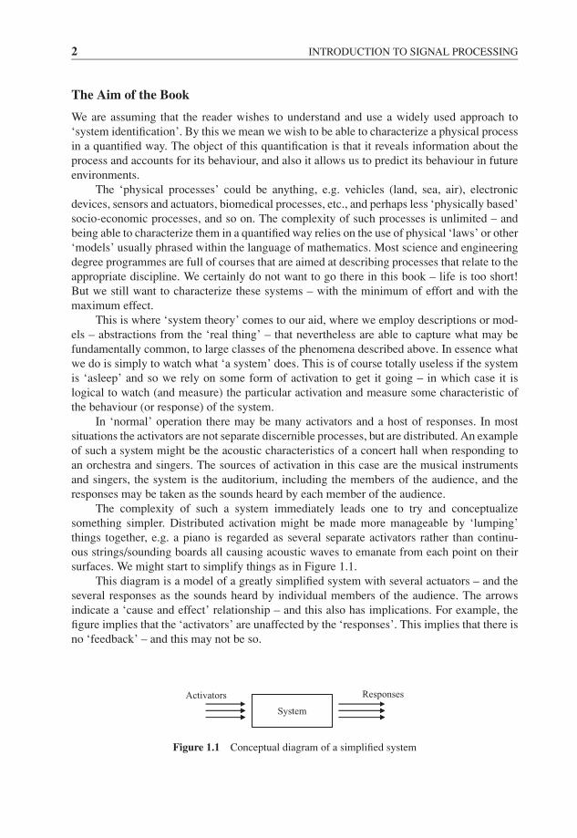
The complexity of such a system immediately leads one to try and conceptualizesomething simpler. Distributed activation might be made more manageable by ‘lumping’things together, e.g. a piano is regarded as several separate activators rather than continu-ous strings/sounding boards all causing acoustic waves to emanate from each point on theirsurfaces. We might start to simplify things as in Figure 1.1.
This diagram is a model of a greatly simplified system with several actuators – and theseveral responses as the sounds heard by individual members of the audience. The arrowsindicate a ‘cause and effect’ relationship – and this also has implications. For example, thefigure implies that the ‘activators’ are unaffected by the ‘responses’. This implies that there isno ‘feedback’ – and this may not be so.
System
Activators Responses
Figure 1.1 Conceptual diagram of a simplified system
JWBK207-01 JWBK207-Shin January 17, 2008 9:36 Char Count= 0
INTRODUCTION TO SIGNAL PROCESSING 3
Systemx(t) y(t)
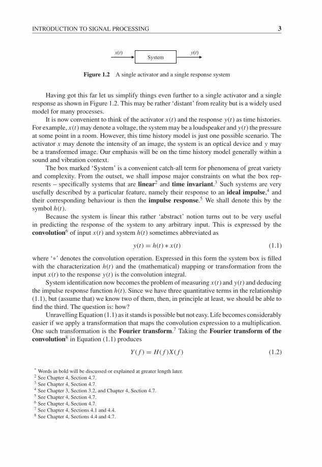
Figure 1.2 A single activator and a single response system
Having got this far let us simplify things even further to a single activator and a singleresponse as shown in Figure 1.2. This may be rather ‘distant’ from reality but is a widely usedmodel for many processes.
It is now convenient to think of the activator x(t) and the response y(t) as time histories.For example, x(t) may denote a voltage, the system may be a loudspeaker and y(t) the pressureat some point in a room. However, this time history model is just one possible scenario. Theactivator x may denote the intensity of an image, the system is an optical device and y maybe a transformed image. Our emphasis will be on the time history model generally within asound and vibration context.
The box marked ‘System’ is a convenient catch-all term for phenomena of great varietyand complexity. From the outset, we shall impose major constraints on what the box rep-resents – specifically systems that are linear2 and time invariant.3 Such systems are veryusefully described by a particular feature, namely their response to an ideal impulse,4 andtheir corresponding behaviour is then the impulse response.5 We shall denote this by thesymbol h(t).
Because the system is linear this rather ‘abstract’ notion turns out to be very usefulin predicting the response of the system to any arbitrary input. This is expressed by theconvolution6 of input x(t) and system h(t) sometimes abbreviated as
y(t) = h(t) ∗ x(t) (1.1)
where ‘*’ denotes the convolution operation. Expressed in this form the system box is filledwith the characterization h(t) and the (mathematical) mapping or transformation from theinput x(t) to the response y(t) is the convolution integral.
System identification now becomes the problem of measuring x(t) and y(t) and deducingthe impulse response function h(t). Since we have three quantitative terms in the relationship(1.1), but (assume that) we know two of them, then, in principle at least, we should be able tofind the third. The question is: how?
Unravelling Equation (1.1) as it stands is possible but not easy. Life becomes considerablyeasier if we apply a transformation that maps the convolution expression to a multiplication.One such transformation is the Fourier transform.7 Taking the Fourier transform of theconvolution8 in Equation (1.1) produces
Y ( f ) = H ( f )X ( f ) (1.2)
* Words in bold will be discussed or explained at greater length later.2 See Chapter 4, Section 4.7.3 See Chapter 4, Section 4.7.4 See Chapter 3, Section 3.2, and Chapter 4, Section 4.7.5 See Chapter 4, Section 4.7.6 See Chapter 4, Section 4.7.7 See Chapter 4, Sections 4.1 and 4.4.8 See Chapter 4, Sections 4.4 and 4.7.
JWBK207-01 JWBK207-Shin January 17, 2008 9:36 Char Count= 0
4 INTRODUCTION TO SIGNAL PROCESSING
where f denotes frequency, and X ( f ), H ( f ) and Y ( f ) are the transforms of x(t), h(t) andy(t). This achieves the unravelling of the input–output relationship as a straightforward mul-tiplication – in a ‘domain’ called the frequency domain.9 In this form the system is char-acterized by the quantity H ( f ) which is called the system frequency response function(FRF).10
The problem of ‘system identification’ now becomes the calculation of H ( f ), whichseems easy: that is, divide Y ( f ) by X ( f ), i.e. divide the Fourier transform of the output by theFourier transform of the input. As long as X ( f ) is never zero this seems to be the end of thestory – but, of course, it is not. Reality interferes in the form of ‘uncertainty’. The measurementsx(t) and y(t) are often not measured perfectly – disturbances or ‘noise’ contaminates them –in which case the result of dividing two transforms of contaminated signals will be of limitedand dubious value.
Also, the actual excitation signal x(t) may itself belong to a class of random11 signals –in which case the straightforward transformation (1.2) also needs more attention. It is this‘dual randomness’ of the actuating (and hence response) signal and additional contaminationthat is addressed in this book.
The Effect of Uncertainty
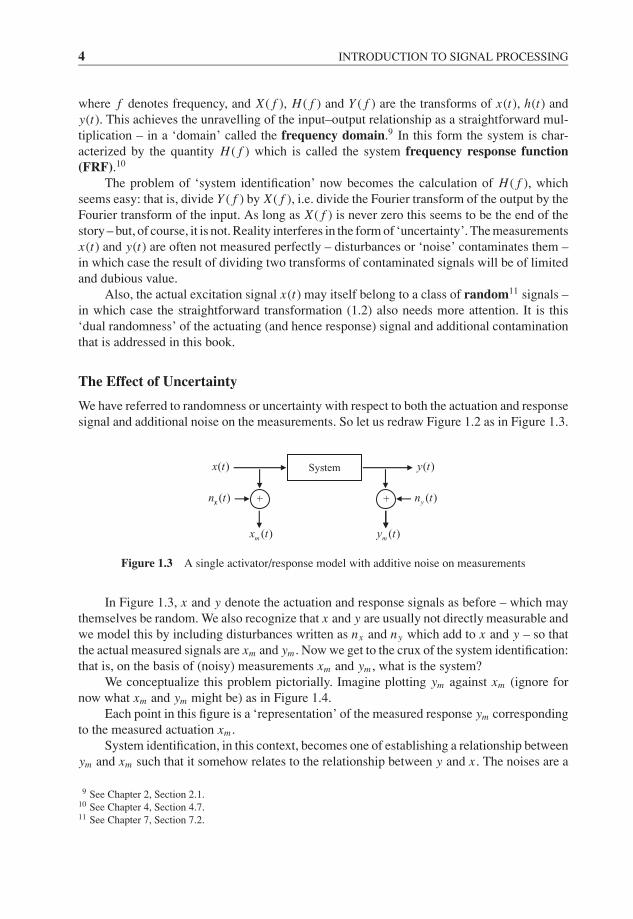
We have referred to randomness or uncertainty with respect to both the actuation and responsesignal and additional noise on the measurements. So let us redraw Figure 1.2 as in Figure 1.3.
System
+
( )x t
+
( )y t
( )yn t( )xn t
( )my t( )mx t
x
Figure 1.3 A single activator/response model with additive noise on measurements
In Figure 1.3, x and y denote the actuation and response signals as before – which maythemselves be random. We also recognize that x and y are usually not directly measurable andwe model this by including disturbances written as nx and ny which add to x and y – so thatthe actual measured signals are xm and ym . Now we get to the crux of the system identification:that is, on the basis of (noisy) measurements xm and ym , what is the system?
We conceptualize this problem pictorially. Imagine plotting ym against xm (ignore fornow what xm and ym might be) as in Figure 1.4.
Each point in this figure is a ‘representation’ of the measured response ym correspondingto the measured actuation xm .
System identification, in this context, becomes one of establishing a relationship betweenym and xm such that it somehow relates to the relationship between y and x . The noises are a
9 See Chapter 2, Section 2.1.10 See Chapter 4, Section 4.7.11 See Chapter 7, Section 7.2.
JWBK207-01 JWBK207-Shin January 17, 2008 9:36 Char Count= 0
INTRODUCTION TO SIGNAL PROCESSING 5
mx
my
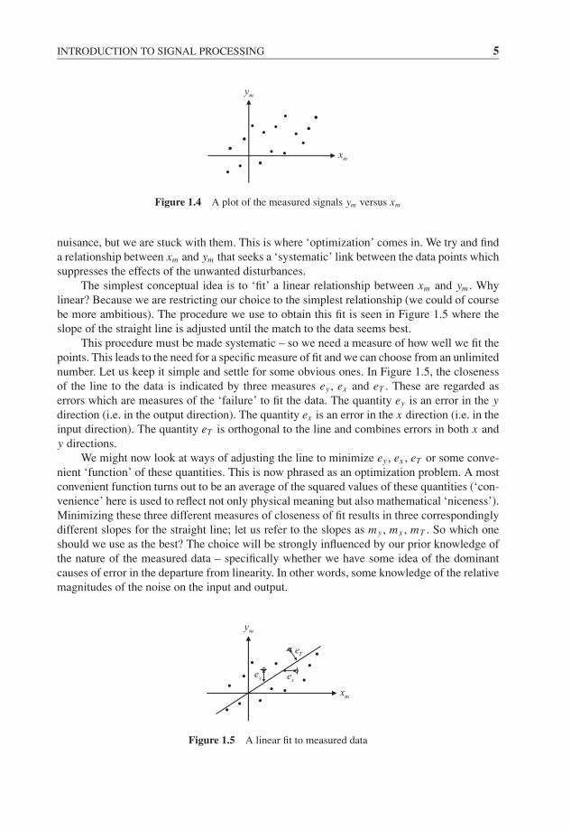
Figure 1.4 A plot of the measured signals ym versus xm
nuisance, but we are stuck with them. This is where ‘optimization’ comes in. We try and finda relationship between xm and ym that seeks a ‘systematic’ link between the data points whichsuppresses the effects of the unwanted disturbances.
The simplest conceptual idea is to ‘fit’ a linear relationship between xm and ym . Whylinear? Because we are restricting our choice to the simplest relationship (we could of coursebe more ambitious). The procedure we use to obtain this fit is seen in Figure 1.5 where theslope of the straight line is adjusted until the match to the data seems best.
This procedure must be made systematic – so we need a measure of how well we fit thepoints. This leads to the need for a specific measure of fit and we can choose from an unlimitednumber. Let us keep it simple and settle for some obvious ones. In Figure 1.5, the closenessof the line to the data is indicated by three measures ey , ex and eT . These are regarded aserrors which are measures of the ‘failure’ to fit the data. The quantity ey is an error in the ydirection (i.e. in the output direction). The quantity ex is an error in the x direction (i.e. in theinput direction). The quantity eT is orthogonal to the line and combines errors in both x andy directions.
We might now look at ways of adjusting the line to minimize ey , ex , eT or some conve-nient ‘function’ of these quantities. This is now phrased as an optimization problem. A mostconvenient function turns out to be an average of the squared values of these quantities (‘con-venience’ here is used to reflect not only physical meaning but also mathematical ‘niceness’).Minimizing these three different measures of closeness of fit results in three correspondinglydifferent slopes for the straight line; let us refer to the slopes as my , mx , mT . So which oneshould we use as the best? The choice will be strongly influenced by our prior knowledge ofthe nature of the measured data – specifically whether we have some idea of the dominantcauses of error in the departure from linearity. In other words, some knowledge of the relativemagnitudes of the noise on the input and output.
xeye
Te
mx
my
Figure 1.5 A linear fit to measured data
JWBK207-01 JWBK207-Shin January 17, 2008 9:36 Char Count= 0
6 INTRODUCTION TO SIGNAL PROCESSING
We could look to the figure for a guide:� my seems best when errors occur on y, i.e. errors on output ey ;� mx seems best when errors occur on x , i.e. errors on input ex ;� mT seems to make an attempt to recognize that errors are on both, i.e. eT .
We might now ask how these rather simple concepts relate to ‘identifying’ the system inFigure 1.3. It turns out that they are directly relevant and lead to three different estimatorsfor the system frequency response function H ( f ). They have come to be referred to in theliterature by the notation H1( f ), H2( f ) and HT ( f ),12 and are the analogues of the slopes my ,mx , mT , respectively.
We have now mapped out what the book is essentially about in Chapters 1 to 10. Thebook ends with a chapter that looks into the implications of multi-input/output systems.
1.1 DESCRIPTIONS OF PHYSICAL DATA (SIGNALS)
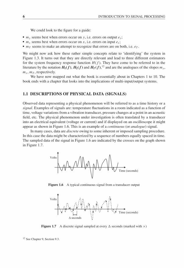
Observed data representing a physical phenomenon will be referred to as a time history or asignal. Examples of signals are: temperature fluctuations in a room indicated as a function oftime, voltage variations from a vibration transducer, pressure changes at a point in an acousticfield, etc. The physical phenomenon under investigation is often translated by a transducerinto an electrical equivalent (voltage or current) and if displayed on an oscilloscope it mightappear as shown in Figure 1.6. This is an example of a continuous (or analogue) signal.
In many cases, data are discrete owing to some inherent or imposed sampling procedure.In this case the data might be characterized by a sequence of numbers equally spaced in time.The sampled data of the signal in Figure 1.6 are indicated by the crosses on the graph shownin Figure 1.7.
Time (seconds)
Volts
Figure 1.6 A typical continuous signal from a transducer output
X
X
X XX
X
X
X
X
X
XX
XX
X
Δ seconds
Time (seconds)
Volts
Figure 1.7 A discrete signal sampled at every � seconds (marked with ×)
12 See Chapter 9, Section 9.3.
JWBK207-01 JWBK207-Shin January 17, 2008 9:36 Char Count= 0
CLASSIFICATION OF DATA 7
Spatial position (ξ)
Road height (h)
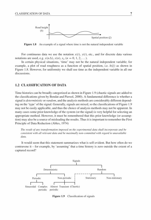
Figure 1.8 An example of a signal where time is not the natural independent variable
For continuous data we use the notation x(t), y(t), etc., and for discrete data variousnotations are used, e.g. x(n�), x(n), xn (n = 0, 1, 2, . . . ).
In certain physical situations, ‘time’ may not be the natural independent variable; forexample, a plot of road roughness as a function of spatial position, i.e. h(ξ ) as shown inFigure 1.8. However, for uniformity we shall use time as the independent variable in all ourdiscussions.
1.2 CLASSIFICATION OF DATA
Time histories can be broadly categorized as shown in Figure 1.9 (chaotic signals are added tothe classifications given by Bendat and Piersol, 2000). A fundamental difference is whether asignal is deterministic or random, and the analysis methods are considerably different depend-ing on the ‘type’ of the signal. Generally, signals are mixed, so the classifications of Figure 1.9may not be easily applicable, and thus the choice of analysis methods may not be apparent. Inmany cases some prior knowledge of the system (or the signal) is very helpful for selecting anappropriate method. However, it must be remembered that this prior knowledge (or assump-tion) may also be a source of misleading the results. Thus it is important to remember the FirstPrinciple of Data Reduction (Ables, 1974)
The result of any transformation imposed on the experimental data shall incorporate and beconsistent with all relevant data and be maximally non-committal with regard to unavailabledata.
It would seem that this statement summarizes what is self-evident. But how often do wecontravene it – for example, by ‘assuming’ that a time history is zero outside the extent of acaptured record?
Signals
Deterministic Random
Periodic Non-periodic Stationary
TransientAlmost
periodic
(Chaotic)
Non-stationary
Complex
periodic
Sinusoidal
Figure 1.9 Classification of signals
JWBK207-01 JWBK207-Shin January 17, 2008 9:36 Char Count= 0
8 INTRODUCTION TO SIGNAL PROCESSING
m
k
x
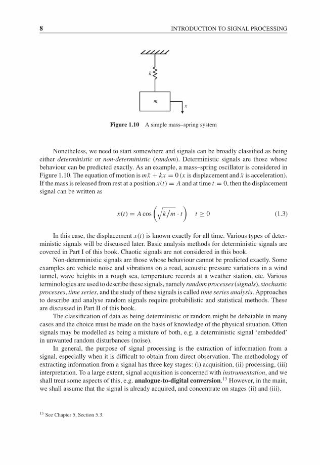
Figure 1.10 A simple mass–spring system
Nonetheless, we need to start somewhere and signals can be broadly classified as beingeither deterministic or non-deterministic (random). Deterministic signals are those whosebehaviour can be predicted exactly. As an example, a mass–spring oscillator is considered inFigure 1.10. The equation of motion is mx + kx = 0 (x is displacement and x is acceleration).If the mass is released from rest at a position x(t) = A and at time t = 0, then the displacementsignal can be written as
x(t) = A cos
(√k/
m · t
)t ≥ 0 (1.3)
In this case, the displacement x(t) is known exactly for all time. Various types of deter-ministic signals will be discussed later. Basic analysis methods for deterministic signals arecovered in Part I of this book. Chaotic signals are not considered in this book.
Non-deterministic signals are those whose behaviour cannot be predicted exactly. Someexamples are vehicle noise and vibrations on a road, acoustic pressure variations in a windtunnel, wave heights in a rough sea, temperature records at a weather station, etc. Variousterminologies are used to describe these signals, namely random processes (signals), stochasticprocesses, time series, and the study of these signals is called time series analysis. Approachesto describe and analyse random signals require probabilistic and statistical methods. Theseare discussed in Part II of this book.
The classification of data as being deterministic or random might be debatable in manycases and the choice must be made on the basis of knowledge of the physical situation. Oftensignals may be modelled as being a mixture of both, e.g. a deterministic signal ‘embedded’in unwanted random disturbances (noise).
In general, the purpose of signal processing is the extraction of information from asignal, especially when it is difficult to obtain from direct observation. The methodology ofextracting information from a signal has three key stages: (i) acquisition, (ii) processing, (iii)interpretation. To a large extent, signal acquisition is concerned with instrumentation, and weshall treat some aspects of this, e.g. analogue-to-digital conversion.13 However, in the main,we shall assume that the signal is already acquired, and concentrate on stages (ii) and (iii).
13 See Chapter 5, Section 5.3.
JWBK207-01 JWBK207-Shin January 17, 2008 9:36 Char Count= 0
CLASSIFICATION OF DATA 9
Piezoceramicpatch actuator
Slender beam
Accelerometer
Force sensor
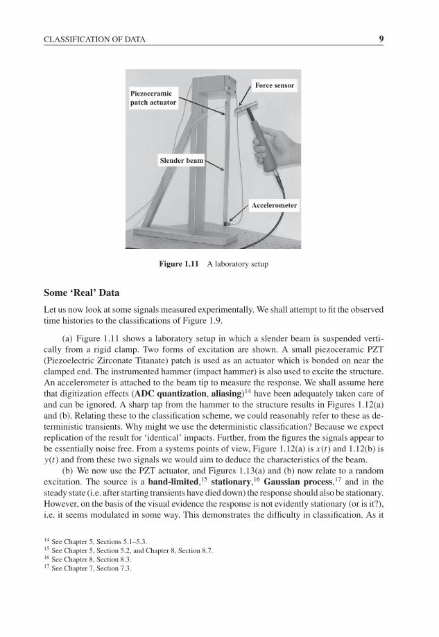
Figure 1.11 A laboratory setup
Some ‘Real’ Data
Let us now look at some signals measured experimentally. We shall attempt to fit the observedtime histories to the classifications of Figure 1.9.
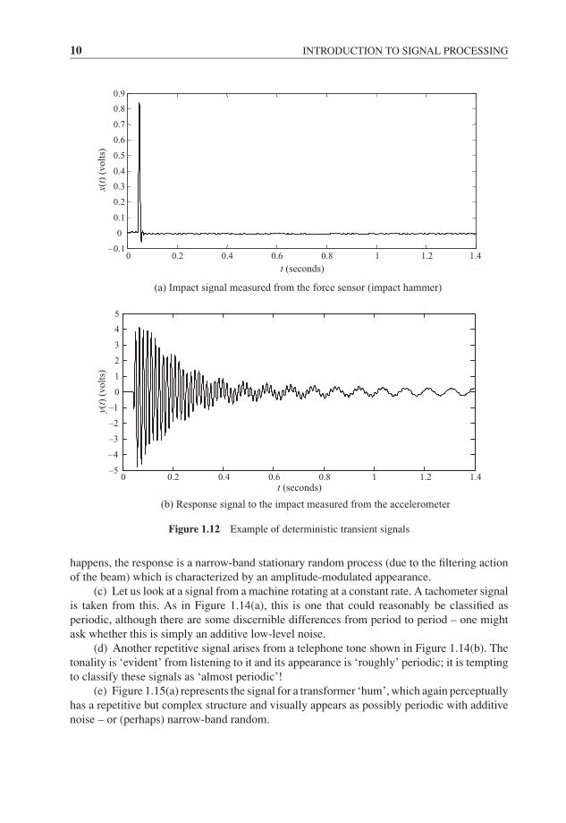
(a) Figure 1.11 shows a laboratory setup in which a slender beam is suspended verti-cally from a rigid clamp. Two forms of excitation are shown. A small piezoceramic PZT(Piezoelectric Zirconate Titanate) patch is used as an actuator which is bonded on near theclamped end. The instrumented hammer (impact hammer) is also used to excite the structure.An accelerometer is attached to the beam tip to measure the response. We shall assume herethat digitization effects (ADC quantization, aliasing)14 have been adequately taken care ofand can be ignored. A sharp tap from the hammer to the structure results in Figures 1.12(a)and (b). Relating these to the classification scheme, we could reasonably refer to these as de-terministic transients. Why might we use the deterministic classification? Because we expectreplication of the result for ‘identical’ impacts. Further, from the figures the signals appear tobe essentially noise free. From a systems points of view, Figure 1.12(a) is x(t) and 1.12(b) isy(t) and from these two signals we would aim to deduce the characteristics of the beam.
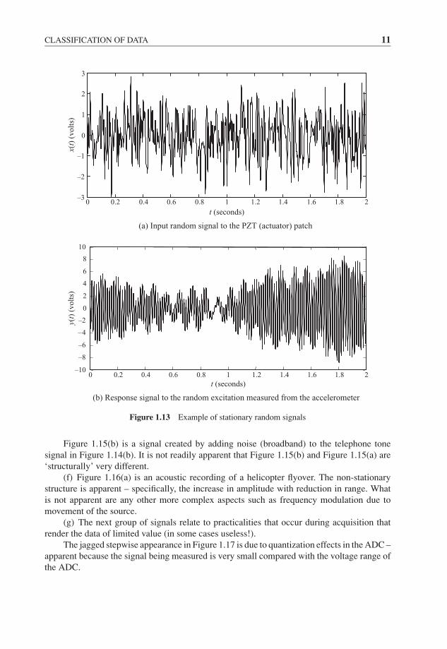
(b) We now use the PZT actuator, and Figures 1.13(a) and (b) now relate to a randomexcitation. The source is a band-limited,15 stationary,16 Gaussian process,17 and in thesteady state (i.e. after starting transients have died down) the response should also be stationary.However, on the basis of the visual evidence the response is not evidently stationary (or is it?),i.e. it seems modulated in some way. This demonstrates the difficulty in classification. As it
14 See Chapter 5, Sections 5.1–5.3.15 See Chapter 5, Section 5.2, and Chapter 8, Section 8.7.16 See Chapter 8, Section 8.3.17 See Chapter 7, Section 7.3.
JWBK207-01 JWBK207-Shin January 17, 2008 9:36 Char Count= 0
10 INTRODUCTION TO SIGNAL PROCESSING
0 0.2 0.4 0.6 0.8 1 1.2 1.4–0.1
0
0.1
0.2
0.3
0.4
0.5
0.6
0.7
0.8
0.9
t (seconds)
(a) Impact signal measured from the force sensor (impact hammer)
x(t)
(volt
s)
0 0.2 0.4 0.6 0.8 1 1.2 1.4–5
–4
–3
–2
–1
0
1
2
3
4
5
t (seconds)
(b) Response signal to the impact measured from the accelerometer
y(t)
(volt
s)
Figure 1.12 Example of deterministic transient signals
happens, the response is a narrow-band stationary random process (due to the filtering actionof the beam) which is characterized by an amplitude-modulated appearance.
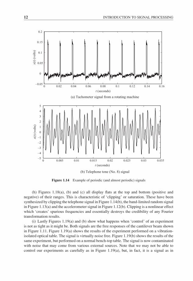
(c) Let us look at a signal from a machine rotating at a constant rate. A tachometer signalis taken from this. As in Figure 1.14(a), this is one that could reasonably be classified asperiodic, although there are some discernible differences from period to period – one mightask whether this is simply an additive low-level noise.
(d) Another repetitive signal arises from a telephone tone shown in Figure 1.14(b). Thetonality is ‘evident’ from listening to it and its appearance is ‘roughly’ periodic; it is temptingto classify these signals as ‘almost periodic’!
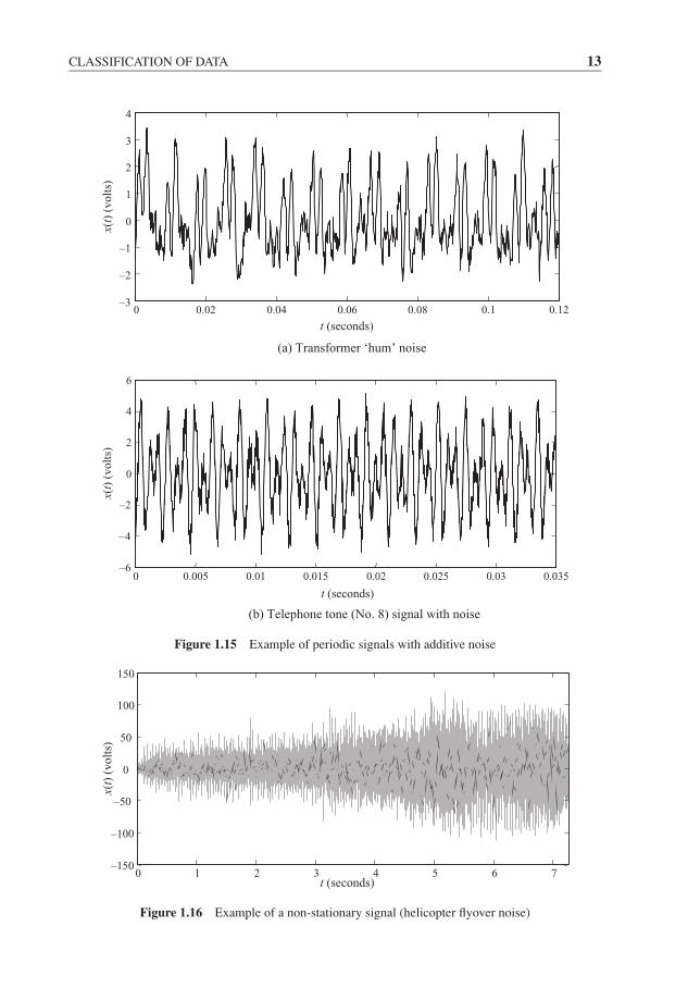
(e) Figure 1.15(a) represents the signal for a transformer ‘hum’, which again perceptuallyhas a repetitive but complex structure and visually appears as possibly periodic with additivenoise – or (perhaps) narrow-band random.
JWBK207-01 JWBK207-Shin January 17, 2008 9:36 Char Count= 0
CLASSIFICATION OF DATA 11
0 0.2 0.4 0.6 0.8 1 1.2 1.4 1.6 1.8 2–3
–2
–1
0
1
2
3
t (seconds)
(a) Input random signal to the PZT (actuator) patch
x(t)
(volt
s)
0 0.2 0.4 0.6 0.8 1 1.2 1.4 1.6 1.8 2–10
–8
–6
–4
–2
0
2
4
6
8
10
t (seconds)
y(t)
(v
olt
s)
(b) Response signal to the random excitation measured from the accelerometer
Figure 1.13 Example of stationary random signals
Figure 1.15(b) is a signal created by adding noise (broadband) to the telephone tonesignal in Figure 1.14(b). It is not readily apparent that Figure 1.15(b) and Figure 1.15(a) are‘structurally’ very different.
(f) Figure 1.16(a) is an acoustic recording of a helicopter flyover. The non-stationarystructure is apparent – specifically, the increase in amplitude with reduction in range. Whatis not apparent are any other more complex aspects such as frequency modulation due tomovement of the source.
(g) The next group of signals relate to practicalities that occur during acquisition thatrender the data of limited value (in some cases useless!).
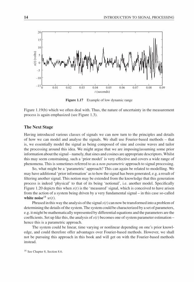
The jagged stepwise appearance in Figure 1.17 is due to quantization effects in the ADC –apparent because the signal being measured is very small compared with the voltage range ofthe ADC.
JWBK207-01 JWBK207-Shin January 17, 2008 9:36 Char Count= 0
12 INTRODUCTION TO SIGNAL PROCESSING
0 0.02 0.04 0.06 0.08 0.1 0.12 0.14 0.16–0.05
0
0.05
0.1
0.15
0.2
t (seconds)
x(t)
(v
olt
s)
(a) Tachometer signal from a rotating machine
0 0.005 0.01 0.015 0.02 0.025 0.03 0.035–5
–4
–3
–2
–1
0
1
2
3
4
5
t (seconds)
x(t)
(v
olt
s)
(b) Telephone tone (No. 8) signal
Figure 1.14 Example of periodic (and almost periodic) signals
(h) Figures 1.18(a), (b) and (c) all display flats at the top and bottom (positive andnegative) of their ranges. This is characteristic of ‘clipping’ or saturation. These have beensynthesized by clipping the telephone signal in Figure 1.14(b), the band-limited random signalin Figure 1.13(a) and the accelerometer signal in Figure 1.12(b). Clipping is a nonlinear effectwhich ‘creates’ spurious frequencies and essentially destroys the credibility of any Fouriertransformation results.
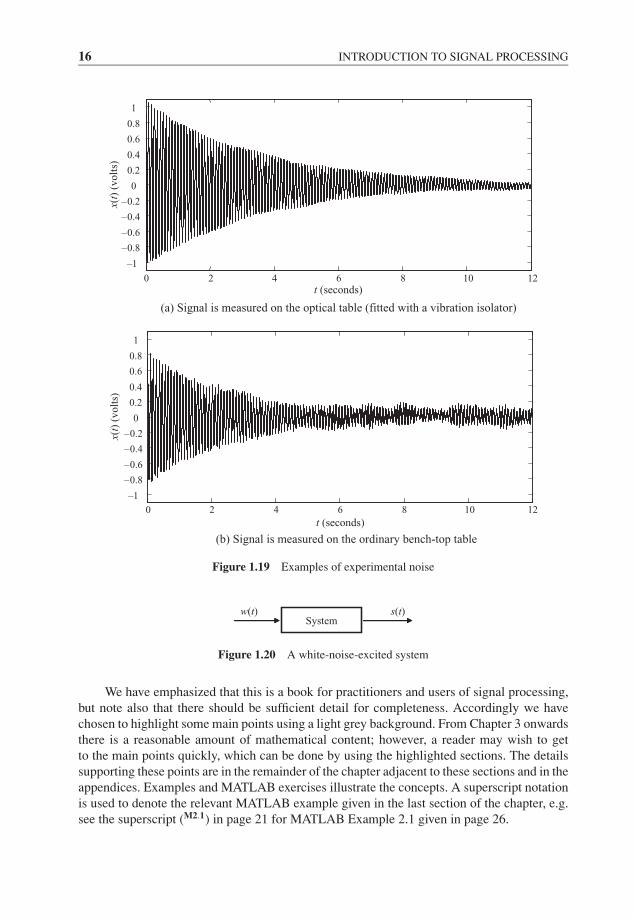
(i) Lastly Figures 1.19(a) and (b) show what happens when ‘control’ of an experimentis not as tight as it might be. Both signals are the free responses of the cantilever beam shownin Figure 1.11. Figure 1.19(a) shows the results of the experiment performed on a vibration-isolated optical table. The signal is virtually noise free. Figure 1.19(b) shows the results of thesame experiment, but performed on a normal bench-top table. The signal is now contaminatedwith noise that may come from various external sources. Note that we may not be able tocontrol our experiments as carefully as in Figure 1.19(a), but, in fact, it is a signal as in
JWBK207-01 JWBK207-Shin January 17, 2008 9:36 Char Count= 0
CLASSIFICATION OF DATA 13
0 0.02 0.04 0.06 0.08 0.1 0.12–3
–2
–1
0
1
2
3
4
t (seconds)
x(t)
(v
olt
s)
(a) Transformer ‘hum’ noise
0 0.005 0.01 0.015 0.02 0.025 0.03 0.035–6
–4
–2
0
2
4
6
t (seconds)
x(t)
(v
olt
s)
(b) Telephone tone (No. 8) signal with noise
Figure 1.15 Example of periodic signals with additive noise
0 1 2 3 4 5 6 7–150
–100
–50
0
50
100
150
t (seconds)
x(t)
(volt
s)
Figure 1.16 Example of a non-stationary signal (helicopter flyover noise)
JWBK207-01 JWBK207-Shin January 17, 2008 9:36 Char Count= 0
14 INTRODUCTION TO SIGNAL PROCESSING
0 0.01 0.02 0.03 0.04 0.05 0.06 0.07 0.08 0.09–15
–10
–5
0
5
10
15
20
t (seconds)
x(t)
(volt
s)
Figure 1.17 Example of low dynamic range
Figure 1.19(b) which we often deal with. Thus, the nature of uncertainty in the measurementprocess is again emphasized (see Figure 1.3).
The Next Stage
Having introduced various classes of signals we can now turn to the principles and detailsof how we can model and analyse the signals. We shall use Fourier-based methods – thatis, we essentially model the signal as being composed of sine and cosine waves and tailorthe processing around this idea. We might argue that we are imposing/assuming some priorinformation about the signal – namely, that sines and cosines are appropriate descriptors. Whilstthis may seem constraining, such a ‘prior model’ is very effective and covers a wide range ofphenomena. This is sometimes referred to as a non-parametric approach to signal processing.
So, what might be a ‘parametric’ approach? This can again be related to modelling. Wemay have additional ‘prior information’ as to how the signal has been generated, e.g. a result offiltering another signal. This notion may be extended from the knowledge that this generationprocess is indeed ‘physical’ to that of its being ‘notional’, i.e. another model. SpecificallyFigure 1.20 depicts this when s(t) is the ‘measured’ signal, which is conceived to have arisenfrom the action of a system being driven by a very fundamental signal – in this case so-calledwhite noise18 w(t).
Phrased in this way the analysis of the signal s(t) can now be transformed into a problem ofdetermining the details of the system. The system could be characterized by a set of parameters,e.g. it might be mathematically represented by differential equations and the parameters are thecoefficients. Set up like this, the analysis of s(t) becomes one of system parameter estimation –hence this is a parametric approach.
The system could be linear, time varying or nonlinear depending on one’s prior knowl-edge, and could therefore offer advantages over Fourier-based methods. However, we shallnot be pursuing this approach in this book and will get on with the Fourier-based methodsinstead.
18 See Chapter 8, Section 8.6.

JWBK207-01 JWBK207-Shin January 17, 2008 9:36 Char Count= 0
CLASSIFICATION OF DATA 15
0 0.005 0.01 0.015 0.02 0.025 0.03 0.035–4
–3
–2
–1
0
1
2
3
4
t (seconds)
x(t)
(v
olt
s)
Clipped
(a) Clipped (almost) periodic signal
0 0.1 0.2 0.3 0.4 0.5 0.6 0.7 0.8 0.9 1–2
–1.5
–1
–0.5
0
0.5
1
1.5
2
t (seconds)
x(t)
(volt
s)
Clipped
(b) Clipped random signal
0 0.2 0.4 0.6 0.8 1 1.2 1.4–3
–2
–1
0
1
2
3
t (seconds)
y(t)
(v
olt
s)
Clipped
(c) Clipped transient signal
Figure 1.18 Examples of clipped signals
JWBK207-01 JWBK207-Shin January 17, 2008 9:36 Char Count= 0
16 INTRODUCTION TO SIGNAL PROCESSING
0 2 4 6 8 10 12
–1
–0.8
–0.6
–0.4
–0.2
0
0.2
0.4
0.6
0.8
1
t (seconds)
x(t)
(v
olt
s)
(a) Signal is measured on the optical table (fitted with a vibration isolator)
0 2 4 6 8 10 12
–1
–0.8
–0.6
–0.4
–0.2
0
0.2
0.4
0.6
0.8
1
t (seconds)
x(t)
(v
olt
s)
(b) Signal is measured on the ordinary bench-top table
Figure 1.19 Examples of experimental noise
Systemw(t) s(t)
Figure 1.20 A white-noise-excited system
We have emphasized that this is a book for practitioners and users of signal processing,but note also that there should be sufficient detail for completeness. Accordingly we havechosen to highlight some main points using a light grey background. From Chapter 3 onwardsthere is a reasonable amount of mathematical content; however, a reader may wish to getto the main points quickly, which can be done by using the highlighted sections. The detailssupporting these points are in the remainder of the chapter adjacent to these sections and in theappendices. Examples and MATLAB exercises illustrate the concepts. A superscript notationis used to denote the relevant MATLAB example given in the last section of the chapter, e.g.see the superscript (M2.1) in page 21 for MATLAB Example 2.1 given in page 26.

JWBK207-02 JWBK207-Shin January 21, 2008 17:32 Char Count= 0
Part IDeterministic Signals
17

JWBK207-02 JWBK207-Shin January 21, 2008 17:32 Char Count= 0
18

JWBK207-02 JWBK207-Shin January 21, 2008 17:32 Char Count= 0
2Classification of Deterministic Data
Introduction
As described in Chapter 1, deterministic signals can be classified as shown in Figure 2.1. Inthis figure, chaotic signals are not considered and the sinusoidal signal and more generalperiodic signals are dealt with together. So deterministic signals are now classified asperiodic, almost periodic and transient, and some basic characteristics are explainedbelow.
TransientAlmost periodic
Deterministic
Periodic Non-periodic
Figure 2.1 Classification of deterministic signals
2.1 PERIODIC SIGNALS
Periodic signals are defined as those whose waveform repeats exactly at regular time intervals.The simplest example is a sinusoidal signal as shown in Figure 2.2(a), where the time intervalfor one full cycle is called the period TP (in seconds) and its reciprocal 1/TP is called thefrequency (in hertz). Another example is a triangular signal (or sawtooth wave), as shown inFigure 2.2(b). This signal has an abrupt change (or discontinuity) every TP seconds. A more
Fundamentals of Signal Processing for Sound and Vibration EngineersK. Shin and J. K. Hammond. C© 2008 John Wiley & Sons, Ltd
19
JWBK207-02 JWBK207-Shin January 21, 2008 17:32 Char Count= 0
20 CLASSIFICATION OF DETERMINISTIC DATA
t
PT
(a) Single sinusoidal signal
(c) General periodic signal
(b) Triangular signal
t
PT
t
PT
Figure 2.2 Examples of periodic signals
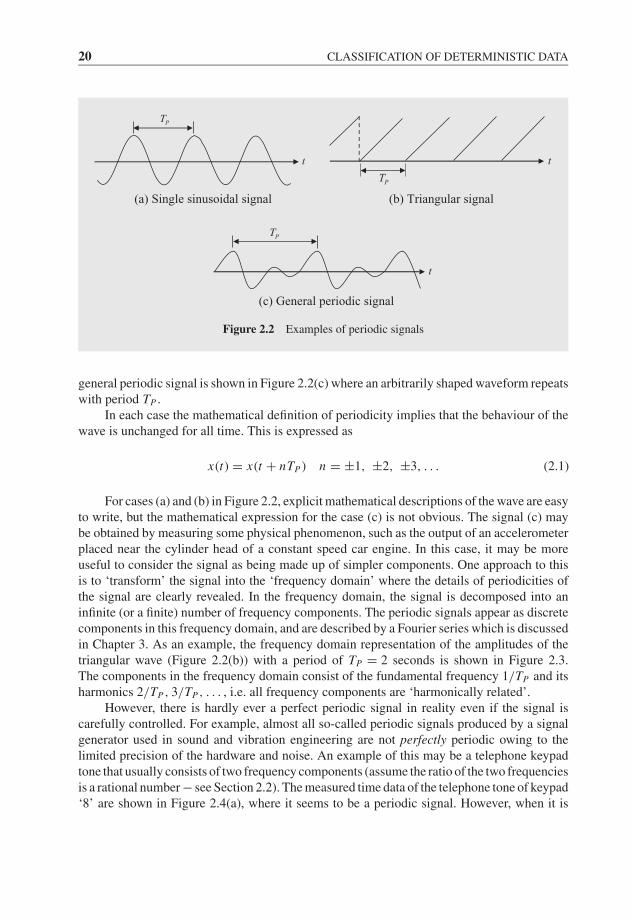
general periodic signal is shown in Figure 2.2(c) where an arbitrarily shaped waveform repeatswith period TP .
In each case the mathematical definition of periodicity implies that the behaviour of thewave is unchanged for all time. This is expressed as
x(t) = x(t + nTP ) n = ±1, ±2, ±3, . . . (2.1)
For cases (a) and (b) in Figure 2.2, explicit mathematical descriptions of the wave are easyto write, but the mathematical expression for the case (c) is not obvious. The signal (c) maybe obtained by measuring some physical phenomenon, such as the output of an accelerometerplaced near the cylinder head of a constant speed car engine. In this case, it may be moreuseful to consider the signal as being made up of simpler components. One approach to thisis to ‘transform’ the signal into the ‘frequency domain’ where the details of periodicities ofthe signal are clearly revealed. In the frequency domain, the signal is decomposed into aninfinite (or a finite) number of frequency components. The periodic signals appear as discretecomponents in this frequency domain, and are described by a Fourier series which is discussedin Chapter 3. As an example, the frequency domain representation of the amplitudes of thetriangular wave (Figure 2.2(b)) with a period of TP = 2 seconds is shown in Figure 2.3.The components in the frequency domain consist of the fundamental frequency 1/TP and itsharmonics 2/TP , 3/TP , . . . , i.e. all frequency components are ‘harmonically related’.
However, there is hardly ever a perfect periodic signal in reality even if the signal iscarefully controlled. For example, almost all so-called periodic signals produced by a signalgenerator used in sound and vibration engineering are not perfectly periodic owing to thelimited precision of the hardware and noise. An example of this may be a telephone keypadtone that usually consists of two frequency components (assume the ratio of the two frequenciesis a rational number − see Section 2.2). The measured time data of the telephone tone of keypad‘8’ are shown in Figure 2.4(a), where it seems to be a periodic signal. However, when it is

JWBK207-02 JWBK207-Shin January 21, 2008 17:32 Char Count= 0
ALMOST PERIODIC SIGNALS 21
0 0.5 1 1.5 2 2.5 3 3.5 4 4.5 50
0.1
0.2
0.3
0.4
0.5
0.6
0.7
0.8
0.9
1
Frequency (Hz)
|cn| (
vo
lts)
1 Hz
PT2
HzPT
d.c. (or mean value) component
Figure 2.3 Frequency domain representation of the amplitudes of a triangular wave with a period ofTp = 2
transformed into the frequency domain, we may find something different. The telephone toneof keypad ‘8’ is designed to have frequency components at 852 Hz and 1336 Hz only. Thismeasured telephone tone is transformed into the frequency domain as shown in Figures 2.4(b)(linear scale) and (c) (log scale). On a linear scale, it seems to be composed of the twofrequencies. However, there are in fact, many other frequency components that may result ifthe signal is not perfectly periodic, and this can be seen by plotting the transform on a logscale as in Figure 2.4(c).
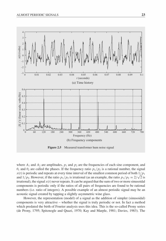
Another practical example of a signal that may be considered to be periodic is transformerhum noise (Figure 2.5(a)) whose dominant frequency components are about 122 Hz, 366 Hzand 488 Hz, as shown in Figure 2.5(b). From Figure 2.5(a), it is apparent that the signal isnot periodic. However, from Figure 2.5(b) it is seen to have a periodic structure contaminatedwith noise.
From the above two practical examples, we note that most periodic signals in practicalsituations are not ‘truly’ periodic, but are ‘almost’ periodic. The term ‘almost periodic’ isdiscussed in the next section.
2.2 ALMOST PERIODIC SIGNALSM2.1 (This superscript is short for MATLAB Example 2.1)
The name ‘almost periodic’ seems self-explanatory and is sometimes called quasi-periodic,i.e. it looks periodic but in fact it is not if observed closely. We shall see in Chapter 3 thatsuitably selected sine and cosine waves may be added together to represent cases (b) and (c)in Figure 2.2. Also, even for apparently simple situations the sum of sines and cosines resultsin a wave which never repeats itself exactly. As an example, consider a wave consisting oftwo sine components as below
x(t) = A1 sin (2πp1t + θ1) + A2 sin (2πp2t + θ2) (2.2)

JWBK207-02 JWBK207-Shin January 21, 2008 17:32 Char Count= 0
22 CLASSIFICATION OF DETERMINISTIC DATA
0 0.005 0.01 0.015 0.02 0.025 0.03 0.035 0.04–5
–3
–1
1
3
5
t (seconds)
(a) Time history
x(t)
(volt
s)
0 0.1 0.2 0.3 0.4 0.5 0.6 0.7 0.8 0.9 1 1.1 1.2 1.3 1.4 1.5 1.6 1.7 1.8 1.9 20
0.1
0.2
0.3
0.4
0.5
0.6
Frequency (kHz)
(b) Frequency components (linear scale)
|X(
f )| (
lin
ear
scal
e, v
olt
s / H
z)v
olt
s/H
z)
10–10
10–8
10–6
10–4
10–2
100
|X(
f )| (
log
sca
le,
vo
lts
0 0.1 0.2 0.3 0.4 0.5 0.6 0.7 0.8 0.9 1 1.1 1.2 1.3 1.4 1.5 1.6 1.7 1.8 1.9 2
Frequency (kHz)
(c) Frequency components (log scale)
Figure 2.4 Measured telephone tone (No. 8) signal considered as periodic
JWBK207-02 JWBK207-Shin January 21, 2008 17:32 Char Count= 0
ALMOST PERIODIC SIGNALS 23
0.010 0.02 0.03 0.04 0.05 0.06 0.07 0.08 0.09 0.1–3
–2
–1
0
1
2
3
4
t (seconds)
(a) Time history
x(t)
(v
olt
s)
0 60 120 180 240 300 360 420 480 540 600 660 720 7800
0.1
0.2
0.3
0.4
0.5
0.6
Frequency (Hz)
(b) Frequency components
|X(
f )| (
linea
r sc
ale,
volt
s/H
z)
Figure 2.5 Measured transformer hum noise signal
where A1 and A2 are amplitudes, p1 and p2 are the frequencies of each sine component, andθ1 and θ2 are called the phases. If the frequency ratio p1/p2 is a rational number, the signalx(t) is periodic and repeats at every time interval of the smallest common period of both 1/p1
and 1/p2. However, if the ratio p1/p2 is irrational (as an example, the ratio p1/p2 = 2/√
2 isirrational), the signal x(t) never repeats. It can be argued that the sum of two or more sinusoidalcomponents is periodic only if the ratios of all pairs of frequencies are found to be rationalnumbers (i.e. ratio of integers). A possible example of an almost periodic signal may be anacoustic signal created by tapping a slightly asymmetric wine glass.
However, the representation (model) of a signal as the addition of simpler (sinusoidal)components is very attractive – whether the signal is truly periodic or not. In fact a methodwhich predated the birth of Fourier analysis uses this idea. This is the so-called Prony series(de Prony, 1795; Spitznogle and Quazi, 1970; Kay and Marple, 1981; Davies, 1983). The
JWBK207-02 JWBK207-Shin January 21, 2008 17:32 Char Count= 0
24 CLASSIFICATION OF DETERMINISTIC DATA
basic components here have the form Ae−σ t sin(ωt + φ) in which there are four parametersfor each component – namely, amplitude A, frequency ω, phase φ and an additional feature σ
which controls the decay of the component.Prony analysis fits a sum of such components to the data using an optimization proce-
dure. The parameters are found from a (nonlinear) algorithm. The nonlinear nature of theoptimization arises because (even if σ = 0) the frequency ω is calculated for each component.This is in contrast to Fourier methods where the frequencies are fixed once the period TP isknown, i.e. only amplitudes and phases are calculated.
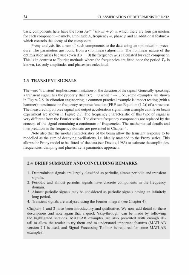
2.3 TRANSIENT SIGNALS
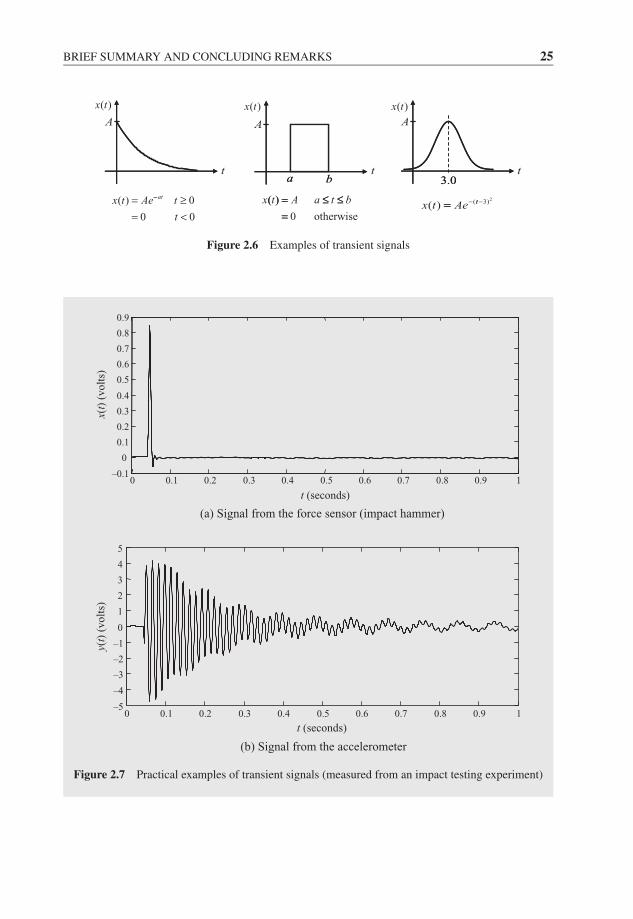
The word ‘transient’ implies some limitation on the duration of the signal. Generally speaking,a transient signal has the property that x(t) = 0 when t → ±∞; some examples are shownin Figure 2.6. In vibration engineering, a common practical example is impact testing (with ahammer) to estimate the frequency response function (FRF, see Equation (1.2)) of a structure.The measured input force signal and output acceleration signal from a simple cantilever beamexperiment are shown in Figure 2.7. The frequency characteristic of this type of signal isvery different from the Fourier series. The discrete frequency components are replaced by theconcept of the signal containing a continuum of frequencies. The mathematical details andinterpretation in the frequency domain are presented in Chapter 4.
Note also that the modal characteristics of the beam allow the transient response to bemodelled as the sum of decaying oscillations, i.e. ideally matched to the Prony series. Thisallows the Prony model to be ‘fitted to’ the data (see Davies, 1983) to estimate the amplitudes,frequencies, damping and phases, i.e. a parametric approach.
2.4 BRIEF SUMMARY AND CONCLUDING REMARKS
1. Deterministic signals are largely classified as periodic, almost periodic and transientsignals.
2. Periodic and almost periodic signals have discrete components in the frequencydomain.
3. Almost periodic signals may be considered as periodic signals having an infinitelylong period.
4. Transient signals are analysed using the Fourier integral (see Chapter 4).
Chapters 1 and 2 have been introductory and qualitative. We now add detail to thesedescriptions and note again that a quick ‘skip-through’ can be made by followingthe highlighted sections. MATLAB examples are also presented with enough de-tail to allow the reader to try them and to understand important features (MATLABversion 7.1 is used, and Signal Processing Toolbox is required for some MATLABexamples).
JWBK207-02 JWBK207-Shin January 21, 2008 17:32 Char Count= 0
BRIEF SUMMARY AND CONCLUDING REMARKS 25
( )x t( )x t( )x t
( ) 0
0 0
atx t Ae t
t
−= ≥= <
( )
0 otherwise
x t A a t b= ≤ ≤=
2( 3)( ) tx t Ae− −=
A A A
t t ta b 3.0
− ( ) = ≤ ≤=
t=
a b 3.0
Figure 2.6 Examples of transient signals
0 0.1 0.2 0.3 0.4 0.5 0.6 0.7 0.8 0.9 1–0.1
0
0.1
0.2
0.3
0.4
0.5
0.6
0.7
0.8
0.9
t (seconds)
x(t)
(v
olt
s)
0 0.1 0.2 0.3 0.4 0.5 0.6 0.7 0.8 0.9 1–5
–4
–3
–2
–1
0
1
2
3
4
5
t (seconds)
y(t)
(v
olt
s)
(a) Signal from the force sensor (impact hammer)
(b) Signal from the accelerometer
Figure 2.7 Practical examples of transient signals (measured from an impact testing experiment)
JWBK207-02 JWBK207-Shin January 21, 2008 17:32 Char Count= 0
26 CLASSIFICATION OF DETERMINISTIC DATA
2.5 MATLAB EXAMPLES1
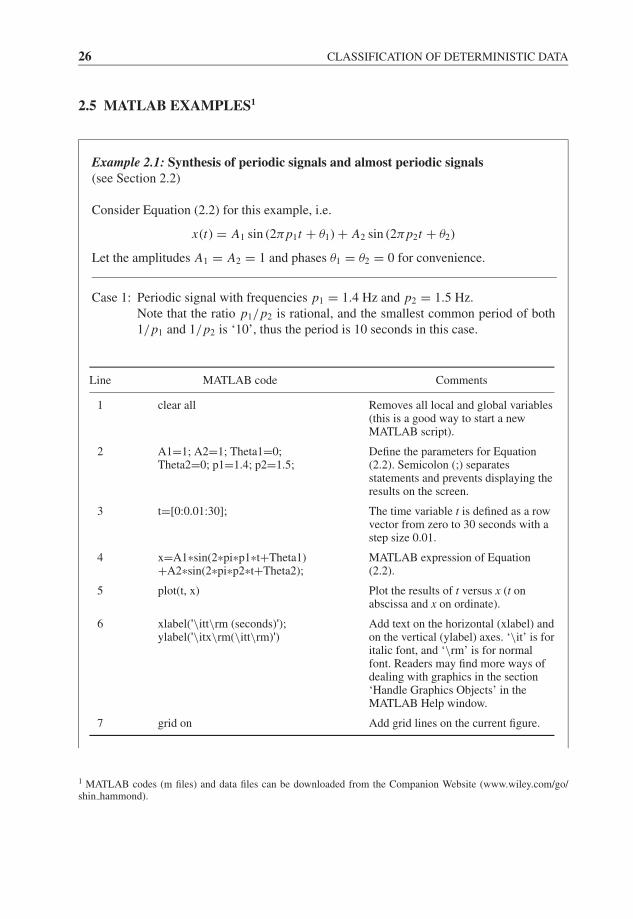
Example 2.1: Synthesis of periodic signals and almost periodic signals(see Section 2.2)
Consider Equation (2.2) for this example, i.e.
x(t) = A1 sin (2πp1t + θ1) + A2 sin (2πp2t + θ2)
Let the amplitudes A1 = A2 = 1 and phases θ1 = θ2 = 0 for convenience.
Case 1: Periodic signal with frequencies p1 = 1.4 Hz and p2 = 1.5 Hz.Note that the ratio p1/p2 is rational, and the smallest common period of both1/p1 and 1/p2 is ‘10’, thus the period is 10 seconds in this case.
Line MATLAB code Comments
1 clear all Removes all local and global variables(this is a good way to start a newMATLAB script).
2 A1=1; A2=1; Theta1=0;Theta2=0; p1=1.4; p2=1.5;
Define the parameters for Equation(2.2). Semicolon (;) separatesstatements and prevents displaying theresults on the screen.
3 t=[0:0.01:30]; The time variable t is defined as a rowvector from zero to 30 seconds with astep size 0.01.
4 x=A1*sin(2*pi*p1*t+Theta1)+A2*sin(2*pi*p2*t+Theta2);
MATLAB expression of Equation(2.2).
5 plot(t, x) Plot the results of t versus x (t onabscissa and x on ordinate).
6 xlabel('\itt\rm (seconds)');ylabel('\itx\rm(\itt\rm)')
Add text on the horizontal (xlabel) andon the vertical (ylabel) axes. ‘\it’ is foritalic font, and ‘\rm’ is for normalfont. Readers may find more ways ofdealing with graphics in the section‘Handle Graphics Objects’ in theMATLAB Help window.
7 grid on Add grid lines on the current figure.
1 MATLAB codes (m files) and data files can be downloaded from the Companion Website (www.wiley.com/go/shin hammond).

JWBK207-02 JWBK207-Shin January 21, 2008 17:32 Char Count= 0
MATLAB EXAMPLES 27
Results
(a) Periodic signal
0 5 10 15 20 25 30–2
–1.5
–1
–0.5
0
0.5
1
1.5
2
t (seconds)
x(t)
Comments: It is clear that this signal is periodic and repeats every 10 seconds, i.e.TP = 10 seconds, thus the fundamental frequency is 0.1 Hz. The frequency domainrepresentation of the above signal is shown in Figure (b). Note that the amplitude ofthe fundamental frequency is zero and thus does not appear in the figure. This ap-plies to subsequent harmonics until 1.4 Hz and 1.5 Hz. Note also that the frequencycomponents 1.4 Hz and 1.5 Hz are ‘harmonically’ related, i.e. both are multiples of0.1 Hz.
0 0.5 1 1.5 2 2.5 3 3.5 4 4.5 50
0.1
0.2
0.3
0.4
0.5
Frequency (Hz)
|X(
f )|
1.4 Hz 1.5 Hz
(b) Fourier transform of x(t) (periodic)
JWBK207-02 JWBK207-Shin January 21, 2008 17:32 Char Count= 0
28 CLASSIFICATION OF DETERMINISTIC DATA
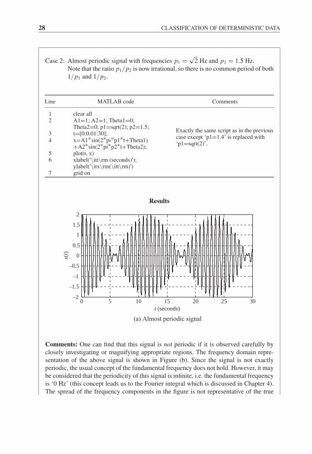
Case 2: Almost periodic signal with frequencies p1 = √2 Hz and p2 = 1.5 Hz.
Note that the ratio p1/p2 is now irrational, so there is no common period of both1/p1 and 1/p2.
Line MATLAB code Comments
1 clear all2 A1=1; A2=1; Theta1=0;
Theta2=0; p1=sqrt(2); p2=1.5;3 t=[0:0.01:30];4 x=A1*sin(2*pi*p1*t+Theta1)
+A2*sin(2*pi*p2*t+Theta2);5 plot(t, x)6 xlabel('\itt\rm (seconds)');
ylabel('\itx\rm(\itt\rm)')7 grid on
Exactly the same script as in the previouscase except ‘p1=1.4’ is replaced with‘p1=sqrt(2)’.
Results
0 5 10 15 20 25 30–2
–1.5
–1
–0.5
0
0.5
1
1.5
2
t (seconds)
x(t)
(a) Almost periodic signal
Comments: One can find that this signal is not periodic if it is observed carefully byclosely investigating or magnifying appropriate regions. The frequency domain repre-sentation of the above signal is shown in Figure (b). Since the signal is not exactlyperiodic, the usual concept of the fundamental frequency does not hold. However, it maybe considered that the periodicity of this signal is infinite, i.e. the fundamental frequencyis ‘0 Hz’ (this concept leads us to the Fourier integral which is discussed in Chapter 4).The spread of the frequency components in the figure is not representative of the true
JWBK207-02 JWBK207-Shin January 21, 2008 17:32 Char Count= 0
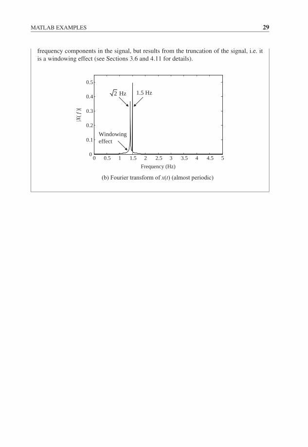
MATLAB EXAMPLES 29
frequency components in the signal, but results from the truncation of the signal, i.e. itis a windowing effect (see Sections 3.6 and 4.11 for details).
0 0.5 1 1.5 2 2.5 3 3.5 4 4.5 50
0.1
0.2
0.3
0.4
0.5
Frequency (Hz)
|X(
f)|
1.5 Hz2 Hz
Windowingeffect
(b) Fourier transform of x(t) (almost periodic)

JWBK207-02 JWBK207-Shin January 21, 2008 17:32 Char Count= 0
30
JWBK207-03 JWBK207-Shin January 26, 2008 16:48 Char Count= 0
3Fourier Series
Introduction
This chapter describes the simplest of the signal types – periodic signals. It begins with theideal situation and the basis of Fourier decomposition, and then, through illustrative examples,discusses some of the practical issues that arise. The delta function is introduced, which isvery useful in signal processing. The chapter concludes with some examples based on theMATLAB software environment.
The presentation is reasonably detailed, but to assist the reader in skipping through tofind the main points being made, some equations and text are highlighted.
3.1 PERIODIC SIGNALS AND FOURIER SERIES
Periodic signals are analysed using Fourier series. The basis of Fourier analysis of aperiodic signal is the representation of such a signal by adding together sine and cosinefunctions of appropriate frequencies, amplitudes and relative phases. For a single sinewave
x(t) = X sin (ωt + φ) = X sin (2π f t + φ) (3.1)
where X is amplitude,ω is circular (angular) frequency in radians per unit time (rad/s),f is (cyclical) frequency in cycles per unit time (Hz),φ is phase angle with respect to the time origin in radians.
The period of this sine wave is TP = 1/ f = 2π/ω seconds. A positive phase angle φ
shifts the waveform to the left (a lead or advance) and a negative phase angle to the right(a lag or delay), where the time shift is φ/ω seconds. When φ = π/2 the wave becomes a
Fundamentals of Signal Processing for Sound and Vibration EngineersK. Shin and J. K. Hammond. C© 2008 John Wiley & Sons, Ltd
31
JWBK207-03 JWBK207-Shin January 26, 2008 16:48 Char Count= 0
32 FOURIER SERIES
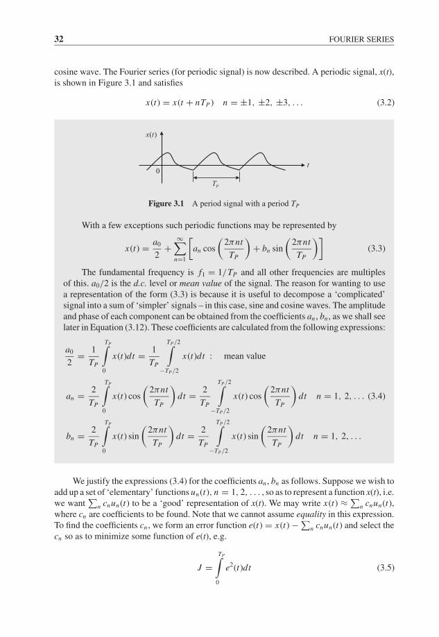
cosine wave. The Fourier series (for periodic signal) is now described. A periodic signal, x(t),is shown in Figure 3.1 and satisfies
x(t) = x(t + nTP ) n = ±1, ±2, ±3, . . . (3.2)
( )x t
t
PT
0
Figure 3.1 A period signal with a period TP
With a few exceptions such periodic functions may be represented by
x(t) = a0
2+
∞∑n=1
[an cos
(2πnt
TP
)+ bn sin
(2πnt
TP
)](3.3)
The fundamental frequency is f1 = 1/TP and all other frequencies are multiplesof this. a0/2 is the d.c. level or mean value of the signal. The reason for wanting to usea representation of the form (3.3) is because it is useful to decompose a ‘complicated’signal into a sum of ‘simpler’ signals – in this case, sine and cosine waves. The amplitudeand phase of each component can be obtained from the coefficients an , bn , as we shall seelater in Equation (3.12). These coefficients are calculated from the following expressions:
a0
2= 1
TP
TP∫0
x(t)dt = 1
TP
TP /2∫−TP /2
x(t)dt : mean value
an = 2
TP
TP∫0
x(t) cos
(2πnt
TP
)dt = 2
TP
TP /2∫−TP /2
x(t) cos
(2πnt
TP
)dt n = 1, 2, . . . (3.4)
bn = 2
TP
TP∫0
x(t) sin
(2πnt
TP
)dt = 2
TP
TP /2∫−TP /2
x(t) sin
(2πnt
TP
)dt n = 1, 2, . . .
We justify the expressions (3.4) for the coefficients an , bn as follows. Suppose we wish toadd up a set of ‘elementary’ functions un(t), n = 1, 2, . . . , so as to represent a function x(t), i.e.we want
∑n cnun(t) to be a ‘good’ representation of x(t). We may write x(t) ≈ ∑
n cnun(t),where cn are coefficients to be found. Note that we cannot assume equality in this expression.To find the coefficients cn , we form an error function e(t) = x(t) − ∑
n cnun(t) and select thecn so as to minimize some function of e(t), e.g.
J =TP∫
0
e2(t)dt (3.5)
JWBK207-03 JWBK207-Shin January 26, 2008 16:48 Char Count= 0
PERIODIC SIGNALS AND FOURIER SERIES 33
Since the un(t) are chosen functions, J is a function of c1, c2, . . . only, so in order to minimizeJ we need necessary conditions as below:
∂ J
∂cm= 0 for m = 1, 2, . . . (3.6)
The function J is
J (c1, c2, . . .) =TP∫
0
(x(t) −
∑n
cnun(t)
)2
dt
and so Equation (3.6) becomes
∂ J
∂cm=
TP∫0
2
(x(t) −
∑n
cnun(t)
)(−um(t))dt = 0 (3.7)
Thus the following result is obtained:
TP∫0
x(t)um(t)dt =∑
n
cn
TP∫0
un(t)um(t)dt (3.8)
At this point we can see that a very desirable property of the ‘basis set’ un is that
TP∫0
un(t)um(t)dt = 0 for n �= m (3.9)
i.e. they should be ‘orthogonal’.Assuming this is so, then using the orthogonal property of Equation (3.9) gives the
required coefficients as
cm =
TP∫0
x(t)um(t)dt
TP∫0
u2m(t)dt
(3.10)
Equation (3.10) is the equivalent of Equation (3.4) for the particular case of selecting sinesand cosines as the basic elements. Specifically Equation (3.4) utilizes the following results oforthogonality:
TP∫0
cos
(2πmt
TP
)sin
(2πnt
TP
)dt = 0 for all m, n
TP∫0
cos
(2πmt
TP
)cos
(2πnt
TP
)dt = 0
TP∫0
sin
(2πmt
TP
)sin
(2πnt
TP
)dt = 0
⎫⎪⎪⎪⎬⎪⎪⎪⎭ for m �= n (3.11)
TP∫0
cos2
(2πnt
TP
)dt =
TP∫0
sin2
(2πnt
TP
)dt = TP
2
JWBK207-03 JWBK207-Shin January 26, 2008 16:48 Char Count= 0
34 FOURIER SERIES
We began by referring to the amplitude and phase of the components of a Fourierseries. This is made explicit now by rewriting Equation (3.3) in the form
x(t) = a0
2+
∞∑n=1
Mn cos (2πn f1t + φn) (3.12)
where f1 = 1/TP is the fundamental frequency,
Mn = √a2
n + b2n are the amplitudes of frequencies at n f1,
φn = tan−1 (−bn/an) are the phases of the frequency components at n f1.
Note that we have assumed that the summation of the components does indeed accuratelyrepresent the signal x(t), i.e. we have tacitly assumed the sum converges, and furthermoreconverges to the signal. This is discussed further in what follows.
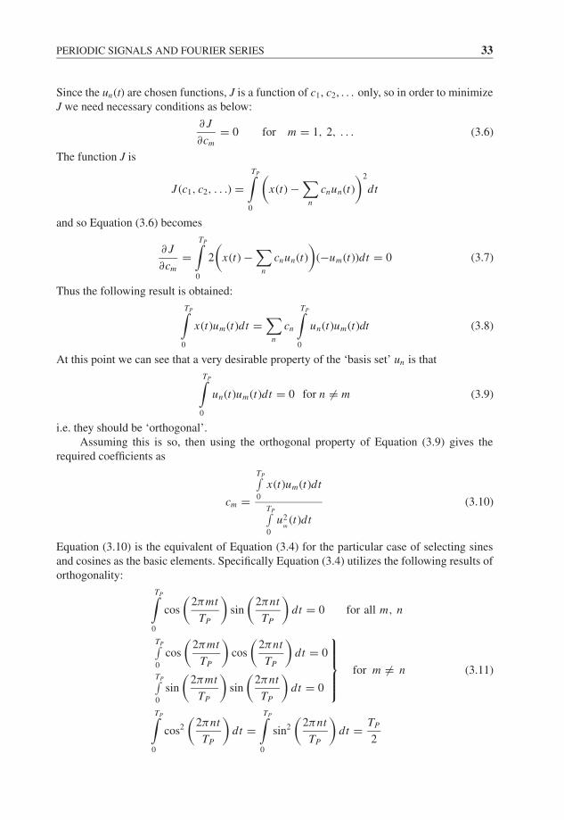
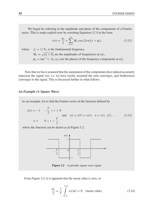
An Example (A Square Wave)
As an example, let us find the Fourier series of the function defined by
x(t) = −1 −T
2< t < 0
and x(t + nT ) = x(t) n = ±1, ±2, . . .
= 1 0 < t <T
2
(3.13)
where the function can be drawn as in Figure 3.2.
2
T−2
Tt
1−
1
( )x t
0
Figure 3.2 A periodic square wave signal
From Figure 3.2, it is apparent that the mean value is zero, so
a0
2= 1
T
T/2∫−T/2
x(t)dt = 0 (mean value) (3.14)
JWBK207-03 JWBK207-Shin January 26, 2008 16:48 Char Count= 0
PERIODIC SIGNALS AND FOURIER SERIES 35
and the coefficients an and bn are
an = 2
T
T/2∫−T/2
x(t) cos
(2πnt
T
)dt
= 2
T
⎡⎢⎣ 0∫−T/2
− cos
(2πnt
T
)dt +
T/2∫0
cos
(2πnt
T
)dt
⎤⎥⎦ = 0
bn = 2
T
T/2∫−T/2
x(t) sin
(2πnt
T
)dt
= 2
T
⎡⎢⎣ 0∫−T/2
− sin
(2πnt
T
)dt +
T/2∫0
sin
(2πnt
T
)dt
⎤⎥⎦ = 2
nπ(1 − cos nπ )
(3.15)
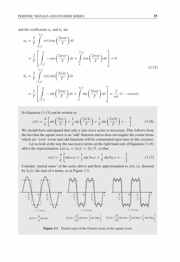
So Equation (3.13) can be written as
x(t) = 4
π
[sin
(2π t
T
)+ 1
3sin
(2π3t
T
)+ 1
5sin
(2π5t
T
)+ · · ·
](3.16)
We should have anticipated that only a sine wave series is necessary. This follows fromthe fact that the square wave is an ‘odd’ function and so does not require the cosine termswhich are ‘even’ (even and odd functions will be commented upon later in this section).
Let us look at the way the successive terms on the right hand side of Equation (3.16)affect the representation. Let ω1 = 2π f1 = 2π/T , so that
x(t) = 4
π
[sin ω1t + 1
3sin 3ω1t + 1
5sin 5ω1t + · · ·
](3.17)
Consider ‘partial sums’ of the series above and their approximation to x(t), i.e. denotedby Sn(t), the sum of n terms, as in Figure 3.3:
2
T−2
T
2
T−2
T−2
T
2
T
1 1
4( ) sinS t tω
π= 2 1 1
4 1( ) sin sin 3
3S t t tω ω
π⎡ ⎤= +⎢ ⎥⎣ ⎦
3 1 1 1
4 1 1( ) sin sin 3 sin 5
3 5S t t t tω ω ω
π⎡ ⎤= + +⎢ ⎥⎣ ⎦
000
Figure 3.3 Partial sums of the Fourier series of the square wave
JWBK207-03 JWBK207-Shin January 26, 2008 16:48 Char Count= 0
36 FOURIER SERIES
nb
f
1
1f
T=
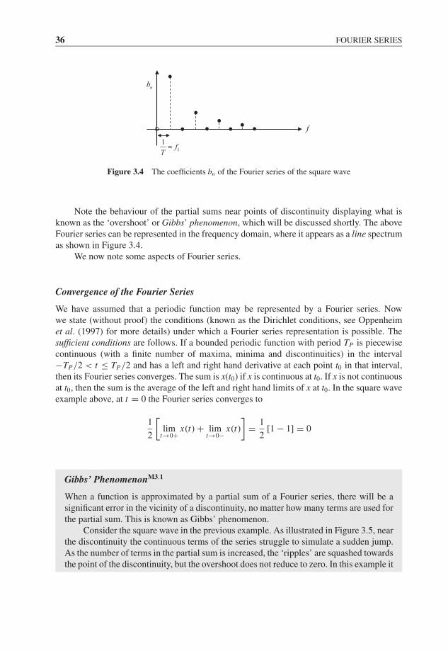
Figure 3.4 The coefficients bn of the Fourier series of the square wave
Note the behaviour of the partial sums near points of discontinuity displaying what isknown as the ‘overshoot’ or Gibbs’ phenomenon, which will be discussed shortly. The aboveFourier series can be represented in the frequency domain, where it appears as a line spectrumas shown in Figure 3.4.
We now note some aspects of Fourier series.
Convergence of the Fourier Series
We have assumed that a periodic function may be represented by a Fourier series. Nowwe state (without proof) the conditions (known as the Dirichlet conditions, see Oppenheimet al. (1997) for more details) under which a Fourier series representation is possible. Thesufficient conditions are follows. If a bounded periodic function with period TP is piecewisecontinuous (with a finite number of maxima, minima and discontinuities) in the interval−TP/2 < t ≤ TP/2 and has a left and right hand derivative at each point t0 in that interval,then its Fourier series converges. The sum is x(t0) if x is continuous at t0. If x is not continuousat t0, then the sum is the average of the left and right hand limits of x at t0. In the square waveexample above, at t = 0 the Fourier series converges to
1
2
[lim
t→0+x(t) + lim
t→0−x(t)
]= 1
2[1 − 1] = 0
Gibbs’ PhenomenonM3.1
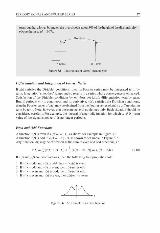
When a function is approximated by a partial sum of a Fourier series, there will be asignificant error in the vicinity of a discontinuity, no matter how many terms are used forthe partial sum. This is known as Gibbs’ phenomenon.
Consider the square wave in the previous example. As illustrated in Figure 3.5, nearthe discontinuity the continuous terms of the series struggle to simulate a sudden jump.As the number of terms in the partial sum is increased, the ‘ripples’ are squashed towardsthe point of the discontinuity, but the overshoot does not reduce to zero. In this example it
JWBK207-03 JWBK207-Shin January 26, 2008 16:48 Char Count= 0
PERIODIC SIGNALS AND FOURIER SERIES 37
turns out that a lower bound on the overshoot is about 9% of the height of the discontinuity(Oppenheim et al., 1997).
Overshoot
7 Terms 20 Terms
Figure 3.5 Illustrations of Gibbs’ phenomenon
Differentiation and Integration of Fourier Series
If x(t) satisfies the Dirichlet conditions, then its Fourier series may be integrated term byterm. Integration ‘smoothes’ jumps and so results in a series whose convergence is enhanced.Satisfaction of the Dirichlet conditions by x(t) does not justify differentiation term by term.But, if periodic x(t) is continuous and its derivative, x(t), satisfies the Dirichlet conditions,then the Fourier series of x(t) may be obtained from the Fourier series of x(t) by differentiatingterm by term. Note, however, that these are general guidelines only. Each situation should beconsidered carefully. For example, the integral of a periodic function for which a0 �= 0 (meanvalue of the signal is not zero) is no longer periodic.
Even and Odd Functions
A function x(t) is even if x(t) = x(−t), as shown for example in Figure 3.6.A function x(t) is odd if x(t) = −x(−t), as shown for example in Figure 3.7.Any function x(t) may be expressed as the sum of even and odd functions, i.e.
x(t) = 1
2[x(t) + x(−t)] + 1
2[x(t) − x(−t)] = xe(t) + xo(t) (3.18)
If x(t) and y(t) are two functions, then the following four properties hold:
1. If x(t) is odd and y(t) is odd, then x(t)·y(t) is even.2. If x(t) is odd and y(t) is even, then x(t)·y(t) is odd.3. If x(t) is even and y(t) is odd, then x(t)·y(t) is odd.4. If x(t) is even and y(t) is even, then x(t)·y(t) is even.
t
Figure 3.6 An example of an even function
JWBK207-03 JWBK207-Shin January 26, 2008 16:48 Char Count= 0
38 FOURIER SERIES
t
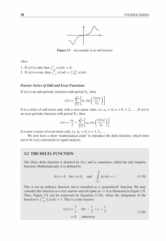
Figure 3.7 An example of an odd function
Also:
1. If x(t) is odd, then∫ a−a x(t)dt = 0.
2. If x(t) is even, then∫ a−a x(t)dt = 2
∫ a0
x(t)dt .
Fourier Series of Odd and Even Functions
If x(t) is an odd periodic function with period TP , then
x(t) =∞∑
n=1
[bn sin
(2πnt
TP
)]It is a series of odd terms only with a zero mean value, i.e. an = 0, n = 0, 1, 2, . . . . If x(t) isan even periodic function with period TP , then
x(t) = a0
2+
∞∑n=1
[an cos
(2πnt
TP
)]It is now a series of even terms only, i.e. bn = 0, n = 1, 2, . . . .
We now have a short ‘mathematical aside’ to introduce the delta function, which turnsout to be very convenient in signal analysis.
3.2 THE DELTA FUNCTION
The Dirac delta function is denoted by δ(t), and is sometimes called the unit impulsefunction. Mathematically, it is defined by
δ(t) = 0 for t �= 0, and
∞∫−∞
δ(t)dt = 1 (3.19)
This is not an ordinary function, but is classified as a ‘generalized’ function. We mayconsider this function as a very narrow and tall spike at t = 0 as illustrated in Figure 3.8.Then, Figure 3.8 can be expressed by Equation (3.20), where the integration of thefunction is
∫ ∞−∞ δε(t)dt = 1. This is a unit impulse:
δε(t) = 1
εfor − ε
2< t <
ε
2
= 0 otherwise
(3.20)

JWBK207-03 JWBK207-Shin January 26, 2008 16:48 Char Count= 0
THE DELTA FUNCTION 39
1ε
2ε− 2εt
Figure 3.8 Model of a unit impulse
Now, if we visualize the spike as infinitesimally narrow, i.e. δ(t) = limε→0 δε(t),then we may represent it on a graph as shown in Figure 3.9, i.e. an arrow whose heightindicates the magnitude of the impulse.
1.0
t
Figure 3.9 Graphical representation of the delta function
An alternative interpretation of the unit impulse is to express it in terms of the unit stepfunction u(t) defined as
u(t) = 1 for t > 0
= 0 for t < 0(3.21)
Since Equation (3.20) can be obtained by using two unit step functions appropriately, i.e.δε(t) = (1/ε) [u (t + ε/2) − u (t − ε/2)], the Dirac delta function and the unit step functionhave the following relationship, which is the Dirac delta function as the derivative of the unitstep function:
δ(t) = limε→0
δε(t) = d
dtu(t) (3.22)
Note that the concept of Equation (3.22) makes it possible to deal with differentiating functionsthat contain discontinuities.
Properties of the Delta Function
A shifted delta function: if a delta function is located at t = a, then it can be written asδ(t − a). Some useful properties of the delta function are:
1. δ(t) = δ(−t), i.e. a delta function is an even function.2. Sifting property: if x(t) is an ‘ordinary’ function, then the integral of the product of the
ordinary function and a shifted delta function is∞∫
−∞x(t)δ(t − a)dt = x(a) (3.23)
i.e. the delta function ‘sifts out’ the value of the ordinary function at t = a.
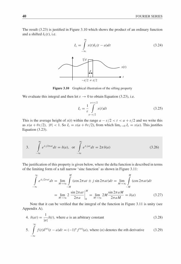
JWBK207-03 JWBK207-Shin January 26, 2008 16:48 Char Count= 0
40 FOURIER SERIES
The result (3.23) is justified in Figure 3.10 which shows the product of an ordinary functionand a shifted δε(t), i.e.
Iε =∞∫
−∞x(t)δε(t − a)dt (3.24)
( )x t
1 ε
ε
2ε− 2εat
Figure 3.10 Graphical illustration of the sifting property
We evaluate this integral and then let ε → 0 to obtain Equation (3.23), i.e.
Iε = 1
ε
a+ε/2∫a−ε/2
x(t)dt (3.25)
This is the average height of x(t) within the range a − ε/2 < t < a + ε/2 and we write thisas x(a + θε/2), |θ | < 1. So Iε = x(a + θε/2), from which limε→0 Iε = x(a). This justifiesEquation (3.23).
3.
∞∫−∞
e± j2πat dt = δ(a), or
∞∫−∞
e± jat dt = 2πδ(a) (3.26)
The justification of this property is given below, where the delta function is described in termsof the limiting form of a tall narrow ‘sinc function’ as shown in Figure 3.11:
∞∫−∞
e± j2πat dt = limM→∞
M∫−M
(cos 2πat ± j sin 2πat)dt = limM→∞
M∫−M
(cos 2πat)dt
= limM→∞
2sin 2πat
2πa
∣∣∣∣M
0
= limM→∞
2Msin 2πaM
2πaM= δ(a) (3.27)
Note that it can be verified that the integral of the function in Figure 3.11 is unity (seeAppendix A).
4. δ(at) = 1
|a|δ(t), where a is an arbitrary constant (3.28)
5.
∞∫−∞
f (t)δ(n)(t − a)dt = (−1)n f (n)(a), where (n) denotes the nth derivative (3.29)
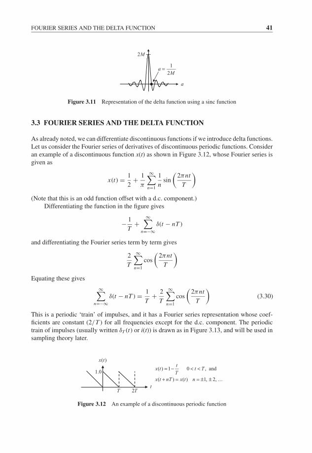
JWBK207-03 JWBK207-Shin January 26, 2008 16:48 Char Count= 0
FOURIER SERIES AND THE DELTA FUNCTION 41
1
2a
M=
a
2M
Figure 3.11 Representation of the delta function using a sinc function
3.3 FOURIER SERIES AND THE DELTA FUNCTION
As already noted, we can differentiate discontinuous functions if we introduce delta functions.Let us consider the Fourier series of derivatives of discontinuous periodic functions. Consideran example of a discontinuous function x(t) as shown in Figure 3.12, whose Fourier series isgiven as
x(t) = 1
2+ 1
π
∞∑n=1
1
nsin
(2πnt
T
)(Note that this is an odd function offset with a d.c. component.)
Differentiating the function in the figure gives
− 1
T+
∞∑n=−∞
δ(t − nT )
and differentiating the Fourier series term by term gives
2
T
∞∑n=1
cos
(2πnt
T
)Equating these gives
∞∑n=−∞
δ(t − nT ) = 1
T+ 2
T
∞∑n=1
cos
(2πnt
T
)(3.30)
This is a periodic ‘train’ of impulses, and it has a Fourier series representation whose coef-ficients are constant (2/T ) for all frequencies except for the d.c. component. The periodictrain of impulses (usually written δT (t) or i(t)) is drawn as in Figure 3.13, and will be used insampling theory later.
( ) 1 0 , and
( ) ( ) 1, 2, ...
tx t t T
Tx t nT x t n
= − < <
+ = = ± ±
( )x t
1.0
T 2Tt
Figure 3.12 An example of a discontinuous periodic function
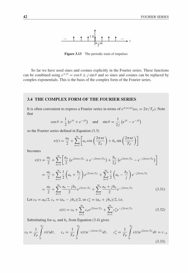
JWBK207-03 JWBK207-Shin January 26, 2008 16:48 Char Count= 0
42 FOURIER SERIES
......t
1.0
T
Figure 3.13 The periodic train of impulses
So far we have used sines and cosines explicitly in the Fourier series. These functionscan be combined using e± jθ = cos θ ± j sin θ and so sines and cosines can be replaced bycomplex exponentials. This is the basis of the complex form of the Fourier series.
3.4 THE COMPLEX FORM OF THE FOURIER SERIES
It is often convenient to express a Fourier series in terms of e± jω1nt (ω1 = 2π/Tp). Notethat
cos θ = 1
2
(e jθ + e− jθ
)and sin θ = 1
2 j
(e jθ − e− jθ
)so the Fourier series defined in Equation (3.3)
x(t) = a0
2+
∞∑n=1
[an cos
(2πnt
TP
)+ bn sin
(2πnt
TP
)]becomes
x(t) = a0
2+
∞∑n=1
[an
2
(e j2πnt/TP + e− j2πnt/TP
) + bn
2 j
(e j2πnt/TP − e− j2πnt/TP
)]
= a0
2+
∞∑n=1
1
2
(an + bn
j
)e j2πnt/TP +
∞∑n=1
1
2
(an − bn
j
)e− j2πnt/TP
= a0
2+
∞∑n=1
an − jbn
2e j2πnt/TP +
∞∑n=1
an + jbn
2e− j2πnt/TP (3.31)
Let c0 = a0/2, cn = (an − jbn)/2, so c∗n = (an + jbn)/2, i.e.
x(t) = c0 +∞∑
n=1
cne j2πnt/TP +∞∑
n=1
c∗ne− j2πnt/TP (3.32)
Substituting for an and bn from Equation (3.4) gives
c0 = 1
TP
TP∫0
x(t)dt, cn = 1
TP
TP∫0
x(t)e− j2πnt/TP dt, c∗n = 1
TP
TP∫0
x(t)e j2πnt/TP dt = c−n
(3.33)
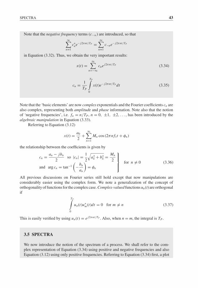
JWBK207-03 JWBK207-Shin January 26, 2008 16:48 Char Count= 0
SPECTRA 43
Note that the negative frequency terms (c−n ) are introduced, so that
∞∑n=1
c∗ne− j2πnt/TP =
∞∑n=1
c−ne− j2πnt/TP
in Equation (3.32). Thus, we obtain the very important results:
x(t) =∞∑
n=−∞cne j2πnt/TP (3.34)
cn = 1
TP
TP∫0
x(t)e− j2πnt/TP dt (3.35)
Note that the ‘basic elements’ are now complex exponentials and the Fourier coefficients cn arealso complex, representing both amplitude and phase information. Note also that the notionof ‘negative frequencies’, i.e. fn = n/TP , n = 0, ±1, ±2, . . . , has been introduced by thealgebraic manipulation in Equation (3.33).
Referring to Equation (3.12)
x(t) = a0
2+
∞∑n=1
Mn cos (2πn f1t + φn)
the relationship between the coefficients is given by
cn = an − jbn
2so |cn| = 1
2
√a2
n + b2n = Mn
2
and arg cn = tan−1
(−bn
an
)= φn
⎫⎪⎪⎬⎪⎪⎭ for n �= 0 (3.36)
All previous discussions on Fourier series still hold except that now manipulations areconsiderably easier using the complex form. We note a generalization of the concept oforthogonality of functions for the complex case. Complex-valued functions un(t) are orthogonalif
TP∫0
un(t)u∗m(t)dt = 0 for m �= n (3.37)
This is easily verified by using un(t) = e j2πnt/TP . Also, when n = m, the integral is TP .
3.5 SPECTRA
We now introduce the notion of the spectrum of a process. We shall refer to the com-plex representation of Equation (3.34) using positive and negative frequencies and alsoEquation (3.12) using only positive frequencies. Referring to Equation (3.34) first, a plot
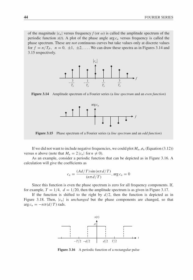
JWBK207-03 JWBK207-Shin January 26, 2008 16:48 Char Count= 0
44 FOURIER SERIES
of the magnitude |cn| versus frequency f (or ω) is called the amplitude spectrum of theperiodic function x(t). A plot of the phase angle arg cn versus frequency is called thephase spectrum. These are not continuous curves but take values only at discrete valuesfor f = n/TP , n = 0, ±1, ±2, . . . . We can draw these spectra as in Figures 3.14 and3.15 respectively.
f
nc
1
PT
3
PT
1
PT−
3
PT−
Figure 3.14 Amplitude spectrum of a Fourier series (a line spectrum and an even function)
arg nc
f
Figure 3.15 Phase spectrum of a Fourier series (a line spectrum and an odd function)
If we did not want to include negative frequencies, we could plot Mn , øn (Equation (3.12))versus n above (note that Mn = 2 |cn| for n �= 0).
As an example, consider a periodic function that can be depicted as in Figure 3.16. Acalculation will give the coefficients as
cn = (Ad/T ) sin (nπd/T )
(nπd/T ), arg cn = 0
Since this function is even the phase spectrum is zero for all frequency components. If,for example, T = 1/4, d = 1/20, then the amplitude spectrum is as given in Figure 3.17.
If the function is shifted to the right by d/2, then the function is depicted as inFigure 3.18. Then, |cn| is unchanged but the phase components are changed, so thatarg cn = −nπ (d/T ) rads.
2T− 2T2d2d−
( )x t
A
t
Figure 3.16 A periodic function of a rectangular pulse
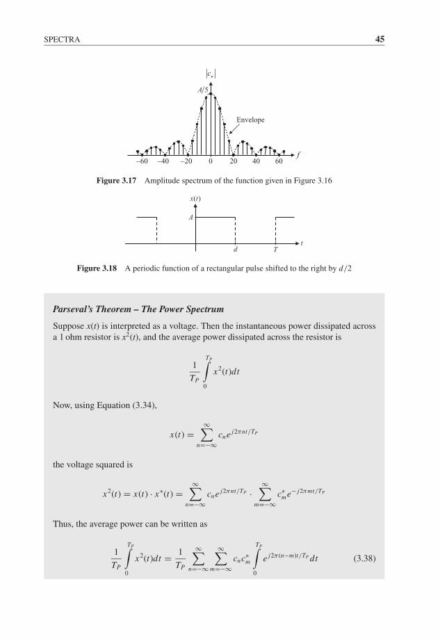
JWBK207-03 JWBK207-Shin January 26, 2008 16:48 Char Count= 0
SPECTRA 45
5A
nc
Envelope
40− 20− 20 40f
060− 60
Figure 3.17 Amplitude spectrum of the function given in Figure 3.16
T
( )x t
A
td
Figure 3.18 A periodic function of a rectangular pulse shifted to the right by d/2
Parseval’s Theorem – The Power Spectrum
Suppose x(t) is interpreted as a voltage. Then the instantaneous power dissipated acrossa 1 ohm resistor is x2(t), and the average power dissipated across the resistor is
1
TP
TP∫0
x2(t)dt
Now, using Equation (3.34),
x(t) =∞∑
n=−∞cne j2πnt/TP
the voltage squared is
x2(t) = x(t) · x∗(t) =∞∑
n=−∞cne j2πnt/TP ·
∞∑m=−∞
c∗me− j2πmt/TP
Thus, the average power can be written as
1
TP
TP∫0
x2(t)dt = 1
TP
∞∑n=−∞
∞∑m=−∞
cnc∗m
TP∫0
e j2π (n−m)t/TP dt (3.38)
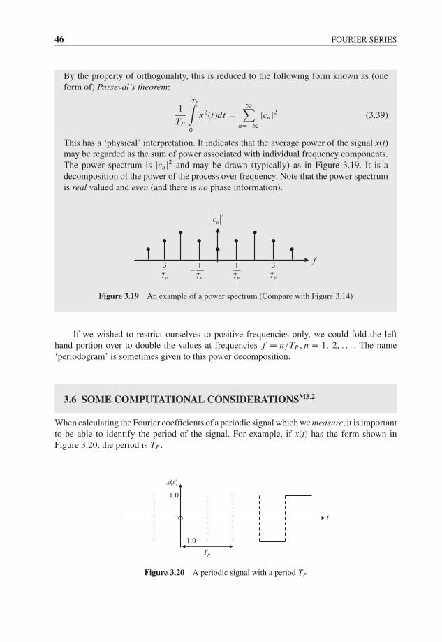
JWBK207-03 JWBK207-Shin January 26, 2008 16:48 Char Count= 0
46 FOURIER SERIES
By the property of orthogonality, this is reduced to the following form known as (oneform of) Parseval’s theorem:
1
TP
TP∫0
x2(t)dt =∞∑
n=−∞|cn|2 (3.39)
This has a ‘physical’ interpretation. It indicates that the average power of the signal x(t)may be regarded as the sum of power associated with individual frequency components.The power spectrum is |cn|2 and may be drawn (typically) as in Figure 3.19. It is adecomposition of the power of the process over frequency. Note that the power spectrumis real valued and even (and there is no phase information).
f
2
nc
1
PT
3
PT
1
PT−3
PT−
Figure 3.19 An example of a power spectrum (Compare with Figure 3.14)
If we wished to restrict ourselves to positive frequencies only, we could fold the lefthand portion over to double the values at frequencies f = n/TP , n = 1, 2, . . . . The name‘periodogram’ is sometimes given to this power decomposition.
3.6 SOME COMPUTATIONAL CONSIDERATIONSM3.2
When calculating the Fourier coefficients of a periodic signal which we measure, it is importantto be able to identify the period of the signal. For example, if x(t) has the form shown inFigure 3.20, the period is TP .
( )x t
t
PT
1.0−
1.0
Figure 3.20 A periodic signal with a period TP
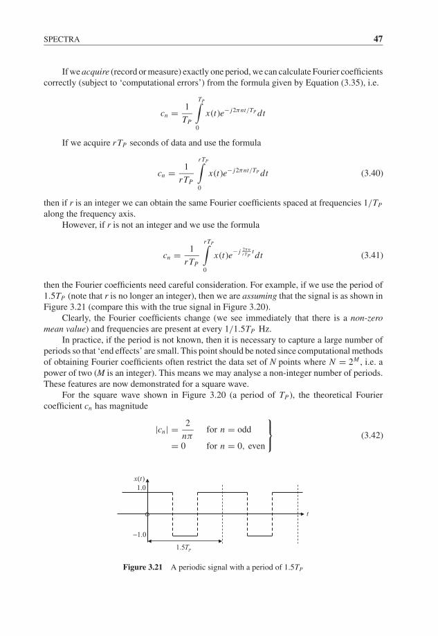
JWBK207-03 JWBK207-Shin January 26, 2008 16:48 Char Count= 0
SPECTRA 47
If we acquire (record or measure) exactly one period, we can calculate Fourier coefficientscorrectly (subject to ‘computational errors’) from the formula given by Equation (3.35), i.e.
cn = 1
TP
TP∫0
x(t)e− j2πnt/TP dt
If we acquire rTP seconds of data and use the formula
cn = 1
rTP
rTP∫0
x(t)e− j2πnt/TP dt (3.40)
then if r is an integer we can obtain the same Fourier coefficients spaced at frequencies 1/TP
along the frequency axis.However, if r is not an integer and we use the formula
cn = 1
rTP
rTP∫0
x(t)e− j 2πnrTP
t dt (3.41)
then the Fourier coefficients need careful consideration. For example, if we use the period of1.5TP (note that r is no longer an integer), then we are assuming that the signal is as shown inFigure 3.21 (compare this with the true signal in Figure 3.20).
Clearly, the Fourier coefficients change (we see immediately that there is a non-zeromean value) and frequencies are present at every 1/1.5TP Hz.
In practice, if the period is not known, then it is necessary to capture a large number ofperiods so that ‘end effects’ are small. This point should be noted since computational methodsof obtaining Fourier coefficients often restrict the data set of N points where N = 2M , i.e. apower of two (M is an integer). This means we may analyse a non-integer number of periods.These features are now demonstrated for a square wave.
For the square wave shown in Figure 3.20 (a period of TP ), the theoretical Fouriercoefficient cn has magnitude
|cn| = 2
nπfor n = odd
= 0 for n = 0, even
⎫⎬⎭ (3.42)
t
1.5 PT
1.0−
1.0
( )x t
Figure 3.21 A periodic signal with a period of 1.5TP
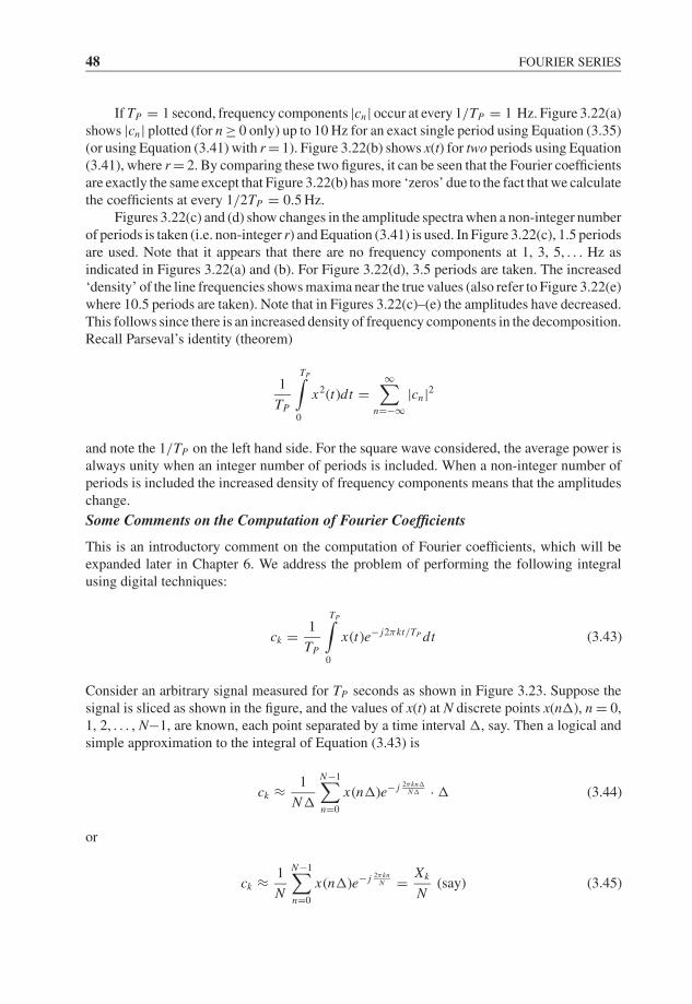
JWBK207-03 JWBK207-Shin January 26, 2008 16:48 Char Count= 0
48 FOURIER SERIES
If TP = 1 second, frequency components |cn| occur at every 1/TP = 1 Hz. Figure 3.22(a)shows |cn| plotted (for n ≥ 0 only) up to 10 Hz for an exact single period using Equation (3.35)(or using Equation (3.41) with r = 1). Figure 3.22(b) shows x(t) for two periods using Equation(3.41), where r = 2. By comparing these two figures, it can be seen that the Fourier coefficientsare exactly the same except that Figure 3.22(b) has more ‘zeros’ due to the fact that we calculatethe coefficients at every 1/2TP = 0.5 Hz.
Figures 3.22(c) and (d) show changes in the amplitude spectra when a non-integer numberof periods is taken (i.e. non-integer r) and Equation (3.41) is used. In Figure 3.22(c), 1.5 periodsare used. Note that it appears that there are no frequency components at 1, 3, 5, . . . Hz asindicated in Figures 3.22(a) and (b). For Figure 3.22(d), 3.5 periods are taken. The increased‘density’ of the line frequencies shows maxima near the true values (also refer to Figure 3.22(e)where 10.5 periods are taken). Note that in Figures 3.22(c)–(e) the amplitudes have decreased.This follows since there is an increased density of frequency components in the decomposition.Recall Parseval’s identity (theorem)
1
TP
TP∫0
x2(t)dt =∞∑
n=−∞|cn|2
and note the 1/TP on the left hand side. For the square wave considered, the average power isalways unity when an integer number of periods is included. When a non-integer number ofperiods is included the increased density of frequency components means that the amplitudeschange.
Some Comments on the Computation of Fourier Coefficients
This is an introductory comment on the computation of Fourier coefficients, which will beexpanded later in Chapter 6. We address the problem of performing the following integralusing digital techniques:
ck = 1
TP
TP∫0
x(t)e− j2πkt/TP dt (3.43)
Consider an arbitrary signal measured for TP seconds as shown in Figure 3.23. Suppose thesignal is sliced as shown in the figure, and the values of x(t) at N discrete points x(n), n = 0,1, 2, . . . , N−1, are known, each point separated by a time interval , say. Then a logical andsimple approximation to the integral of Equation (3.43) is
ck ≈ 1
N
N−1∑n=0
x(n)e− j 2πknN · (3.44)
or
ck ≈ 1
N
N−1∑n=0
x(n)e− j 2πknN = Xk
N(say) (3.45)
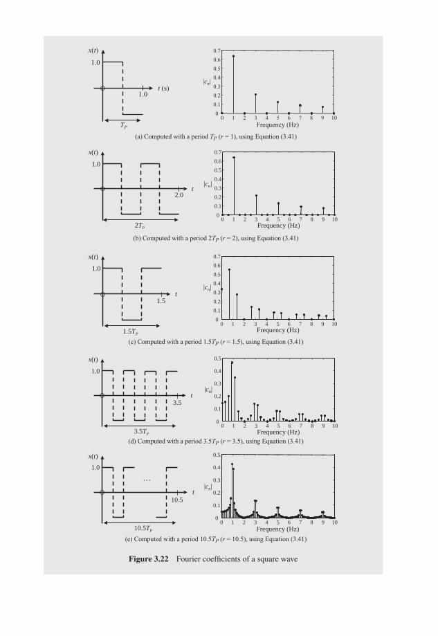
JWBK207-03 JWBK207-Shin January 26, 2008 16:48 Char Count= 0
x(t)
t (s)
TP
1.0
1.0
0 1 2 3 4 5 6 7 8 9 100
0.1
0.2
0.3
0.4
0.5
0.6
0.7
|cn|
Frequency (Hz)
(a) Computed with a period TP (r = 1), using Equation (3.41)
(b) Computed with a period 2TP (r = 2), using Equation (3.41)
(c) Computed with a period 1.5TP (r = 1.5), using Equation (3.41)
(d) Computed with a period 3.5TP (r = 3.5), using Equation (3.41)
(e) Computed with a period 10.5TP (r = 10.5), using Equation (3.41)
x(t)
t
2TP
2.0
1.0
|cn|
Frequency (Hz)0 1 2 3 4 5 6 7 8 9 10
0
0.1
0.2
0.3
0.4
0.5
0.6
0.7
x(t)
t
1.5TP
1.5
1.0
0.7
|cn|
Frequency (Hz)0 1 2 3 4 5 6 7 8 9 10
0
0.1
0.2
0.3
0.4
0.5
0.6
x(t)
t
3.5TP
3.5
1.0
|cn|
Frequency (Hz)0 1 2 3 4 5 6 7 8 9 10
0
0.1
0.2
0.3
0.4
0.5
x(t)
t
10.5TP
10.5
…1.0
|cn|
Frequency (Hz)0 1 2 3 4 5 6 7 8 9 10
0
0.1
0.2
0.3
0.4
0.5
Figure 3.22 Fourier coefficients of a square wave
49
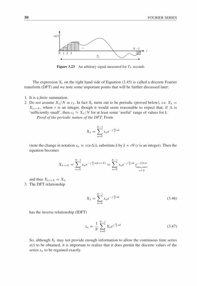
JWBK207-03 JWBK207-Shin January 26, 2008 16:48 Char Count= 0
50 FOURIER SERIES
……t
PT
1N −
( )x t
0 1 2 3
Figure 3.23 An arbitrary signal measured for TP seconds
The expression Xk on the right hand side of Equation (3.45) is called a discrete Fouriertransform (DFT) and we note some important points that will be further discussed later:
1. It is a finite summation.2. Do not assume Xk/N ≡ ck . In fact Xk turns out to be periodic (proved below), i.e. Xk =
Xk+r N , where r is an integer, though it would seem reasonable to expect that, if is‘sufficiently small’, then ck ≈ Xk/N for at least some ‘useful’ range of values for k.
Proof of the periodic nature of the DFT: From
Xk =N−1∑n=0
xne− j 2πN nk
(note the change in notation xn ≡ x(n)), substitute k by k + rN (r is an integer). Then theequation becomes
Xk+r N =N−1∑n=0
xne− j 2πN n(k+r N ) =
N−1∑n=0
xne− j 2πN nk e− j2πnr︸ ︷︷ ︸
=1.0
and thus Xk+r N = Xk .3. The DFT relationship
Xk =N−1∑n=0
xne− j 2πN nk (3.46)
has the inverse relationship (IDFT)
xn = 1
N
N−1∑k=0
Xke j 2πN nk (3.47)
So, although Xk may not provide enough information to allow the continuous time seriesx(t) to be obtained, it is important to realize that it does permit the discrete values of theseries xn to be regained exactly.
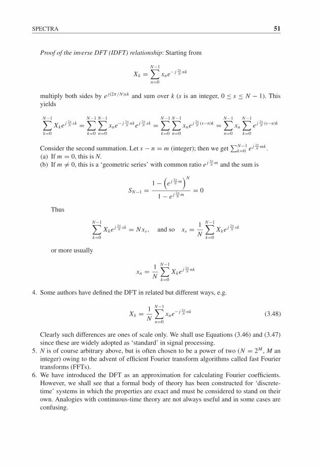
JWBK207-03 JWBK207-Shin January 26, 2008 16:48 Char Count= 0
SPECTRA 51
Proof of the inverse DFT (IDFT) relationship: Starting from
Xk =N−1∑n=0
xne− j 2πN nk
multiply both sides by e j(2π/N )sk and sum over k (s is an integer, 0 ≤ s ≤ N − 1). Thisyields
N−1∑k=0
Xke j 2πN sk =
N−1∑k=0
N−1∑n=0
xne− j 2πN nke j 2π
N sk =N−1∑k=0
N−1∑n=0
xne j 2πN (s−n)k =
N−1∑n=0
xn
N−1∑k=0
e j 2πN (s−n)k
Consider the second summation. Let s − n = m (integer); then we get∑N−1
k=0 e j 2πN mk .
(a) If m = 0, this is N.(b) If m �= 0, this is a ‘geometric series’ with common ratio e j 2π
N m and the sum is
SN−1 =1 −
(e j 2π
N m)N
1 − e j 2πN m
= 0
Thus
N−1∑k=0
Xke j 2πN sk = N xs, and so xs = 1
N
N−1∑k=0
Xke j 2πN sk
or more usually
xn = 1
N
N−1∑k=0
Xke j 2πN nk
4. Some authors have defined the DFT in related but different ways, e.g.
Xk = 1
N
N−1∑n=0
xne− j 2πN nk (3.48)
Clearly such differences are ones of scale only. We shall use Equations (3.46) and (3.47)since these are widely adopted as ‘standard’ in signal processing.
5. N is of course arbitrary above, but is often chosen to be a power of two (N = 2M , M aninteger) owing to the advent of efficient Fourier transform algorithms called fast Fouriertransforms (FFTs).
6. We have introduced the DFT as an approximation for calculating Fourier coefficients.However, we shall see that a formal body of theory has been constructed for ‘discrete-time’ systems in which the properties are exact and must be considered to stand on theirown. Analogies with continuous-time theory are not always useful and in some cases areconfusing.
JWBK207-03 JWBK207-Shin January 26, 2008 16:48 Char Count= 0
52 FOURIER SERIES
3.7 BRIEF SUMMARY
1. A periodic signal of period TP may be expressed (Equations (3.34) and (3.35)) by
x(t) =∞∑
n=−∞cne j2πnt/TP with cn = 1
TP
TP∫0
x(t)e− j2πnt/TP dt
2. The plots of |cn| versus frequency and arg cn versus frequency are amplitude and phase(line) spectra of the Fourier decomposition.
3. The average power of a periodic signal is described by Equation (3.39), i.e.
1
TP
TP∫0
x2(t)dt =∞∑
n=−∞|cn|2 Parseval’s theorem (identity)
A plot of |cn|2 versus frequency is called a power spectrum (or a periodogram).4. The DFT and IDFT relationships for discrete data are defined by Equations (3.46) and
(3.47),
Xk =N−1∑n=0
xne− j 2πN nk and xn = 1
N
N−1∑k=0
Xke j 2πN nk
The Fourier coefficients ck are approximated by ck ≈ Xk/N if an integer number ofperiods is taken and only for a restricted range of k.
We now include some MATLAB examples illustrating the material covered.
3.8 MATLAB EXAMPLES
Example 3.1: Illustration of the convergence of the Fourier series and Gibbs’phenomenon (see Section 3.1)
Consider Equation (3.17),
x(t) = 4
π
[sin ω1t + 1
3sin 3ω1t + 1
5sin 5ω1t + · · ·
]In this MATLAB example, we compare the results of 3, 7 and 20 partial sums inEquation (3.17).
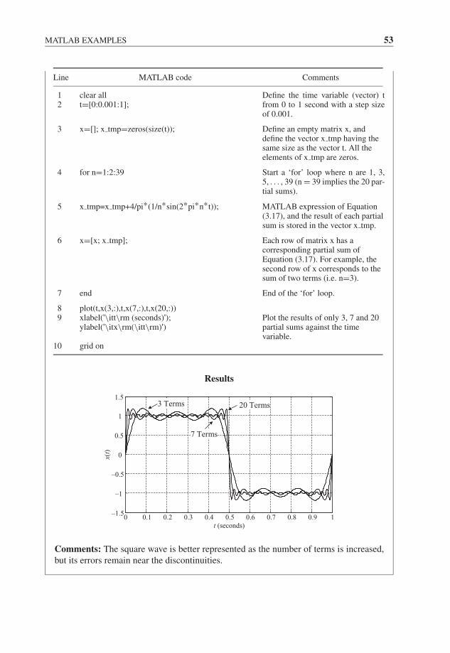
JWBK207-03 JWBK207-Shin January 26, 2008 16:48 Char Count= 0
MATLAB EXAMPLES 53
Line MATLAB code Comments
12
clear allt=[0:0.001:1];
Define the time variable (vector) tfrom 0 to 1 second with a step sizeof 0.001.
3 x=[]; x tmp=zeros(size(t)); Define an empty matrix x, anddefine the vector x tmp having thesame size as the vector t. All theelements of x tmp are zeros.
4 for n=1:2:39 Start a ‘for’ loop where n are 1, 3,5, . . . , 39 (n = 39 implies the 20 par-tial sums).
5 x tmp=x tmp+4/pi*(1/n*sin(2*pi*n*t)); MATLAB expression of Equation(3.17), and the result of each partialsum is stored in the vector x tmp.
6 x=[x; x tmp]; Each row of matrix x has acorresponding partial sum ofEquation (3.17). For example, thesecond row of x corresponds to thesum of two terms (i.e. n=3).
7 end End of the ‘for’ loop.
8 plot(t,x(3,:),t,x(7,:),t,x(20,:))9 xlabel('\itt\rm (seconds)');
ylabel('\itx\rm(\itt\rm)')Plot the results of only 3, 7 and 20partial sums against the timevariable.
10 grid on
Results
0 0.1 0.2 0.3 0.4 0.5 0.6 0.7 0.8 0.9 1–1.5
–1
–0.5
0
0.5
1
1.5
t (seconds)
x(t)
7 Terms
3 Terms 20 Terms
Comments: The square wave is better represented as the number of terms is increased,but its errors remain near the discontinuities.
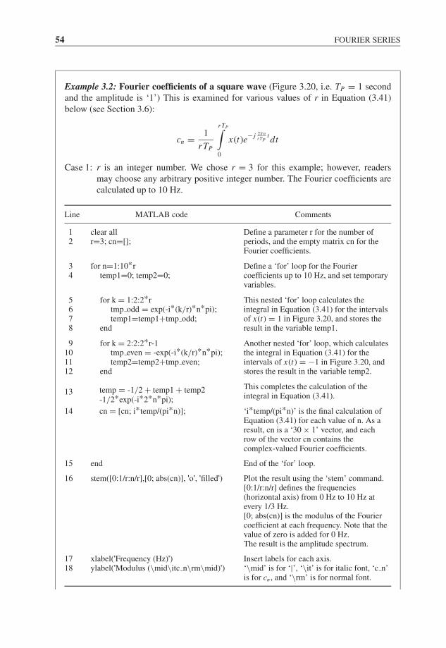
JWBK207-03 JWBK207-Shin January 26, 2008 16:48 Char Count= 0
54 FOURIER SERIES
Example 3.2: Fourier coefficients of a square wave (Figure 3.20, i.e. TP = 1 secondand the amplitude is ‘1’) This is examined for various values of r in Equation (3.41)below (see Section 3.6):
cn = 1
rTP
rTP∫0
x(t)e− j 2πnrTP
t dt
Case 1: r is an integer number. We chose r = 3 for this example; however, readersmay choose any arbitrary positive integer number. The Fourier coefficients arecalculated up to 10 Hz.
Line MATLAB code Comments
12
clear allr=3; cn=[];
Define a parameter r for the number ofperiods, and the empty matrix cn for theFourier coefficients.
34
for n=1:10*rtemp1=0; temp2=0;
Define a ‘for’ loop for the Fouriercoefficients up to 10 Hz, and set temporaryvariables.
5678
for k = 1:2:2*rtmp odd = exp(-i*(k/r)*n*pi);temp1=temp1+tmp odd;
end
This nested ‘for’ loop calculates theintegral in Equation (3.41) for the intervalsof x(t) = 1 in Figure 3.20, and stores theresult in the variable temp1.
9101112
for k = 2:2:2*r-1tmp even = -exp(-i*(k/r)*n*pi);temp2=temp2+tmp even;
end
Another nested ‘for’ loop, which calculatesthe integral in Equation (3.41) for theintervals of x(t) = −1 in Figure 3.20, andstores the result in the variable temp2.
13 temp = -1/2 + temp1 + temp2-1/2*exp(-i*2*n*pi);
This completes the calculation of theintegral in Equation (3.41).
14 cn = [cn; i*temp/(pi*n)]; ‘i*temp/(pi*n)’ is the final calculation ofEquation (3.41) for each value of n. As aresult, cn is a ‘30 × 1’ vector, and eachrow of the vector cn contains thecomplex-valued Fourier coefficients.
15 end End of the ‘for’ loop.
16 stem([0:1/r:n/r],[0; abs(cn)], 'o', 'filled') Plot the result using the ‘stem’ command.[0:1/r:n/r] defines the frequencies(horizontal axis) from 0 Hz to 10 Hz atevery 1/3 Hz.[0; abs(cn)] is the modulus of the Fouriercoefficient at each frequency. Note that thevalue of zero is added for 0 Hz.The result is the amplitude spectrum.
17 xlabel('Frequency (Hz)') Insert labels for each axis.18 ylabel('Modulus (\mid\itc n\rm\mid)') ‘\mid’ is for ‘|’, ‘\it’ is for italic font, ‘c n’
is for cn , and ‘\rm’ is for normal font.
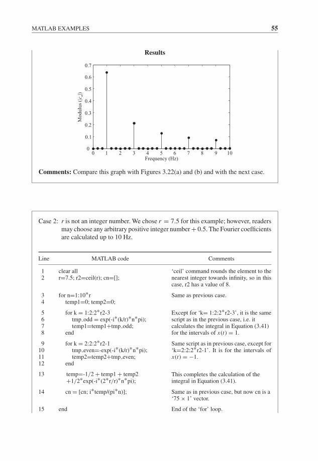
JWBK207-03 JWBK207-Shin January 26, 2008 16:48 Char Count= 0
MATLAB EXAMPLES 55
Results
0
0.1
0.2
0.3
0.4
0.5
0.6
0.7
Mo
du
lus
(|c n|
)
0 1 2 3 4 5 6 7 8 9 10Frequency (Hz)
Comments: Compare this graph with Figures 3.22(a) and (b) and with the next case.
Case 2: r is not an integer number. We chose r = 7.5 for this example; however, readersmay choose any arbitrary positive integer number + 0.5. The Fourier coefficientsare calculated up to 10 Hz.
Line MATLAB code Comments
12
clear allr=7.5; r2=ceil(r); cn=[];
‘ceil’ command rounds the element to thenearest integer towards infinity, so in thiscase, r2 has a value of 8.
34
for n=1:10*rtemp1=0; temp2=0;
Same as previous case.
5678
for k = 1:2:2*r2-3tmp odd = exp(-i*(k/r)*n*pi);temp1=temp1+tmp odd;
end
Except for ‘k= 1:2:2*r2-3’, it is the samescript as in the previous case, i.e. itcalculates the integral in Equation (3.41)for the intervals of x(t) = 1.
9101112
for k = 2:2:2*r2-1tmp even=-exp(-i*(k/r)*n*pi);temp2=temp2+tmp even;
end
Same script as in previous case, except for‘k=2:2:2*r2-1’. It is for the intervals ofx(t) = −1.
13 temp=-1/2 + temp1 + temp2+1/2*exp(-i*(2*r/r)*n*pi);
This completes the calculation of theintegral in Equation (3.41).
14 cn = [cn; i*temp/(pi*n)]; Same as in previous case, but now cn is a‘75 × 1’ vector.
15 end End of the ‘for’ loop.
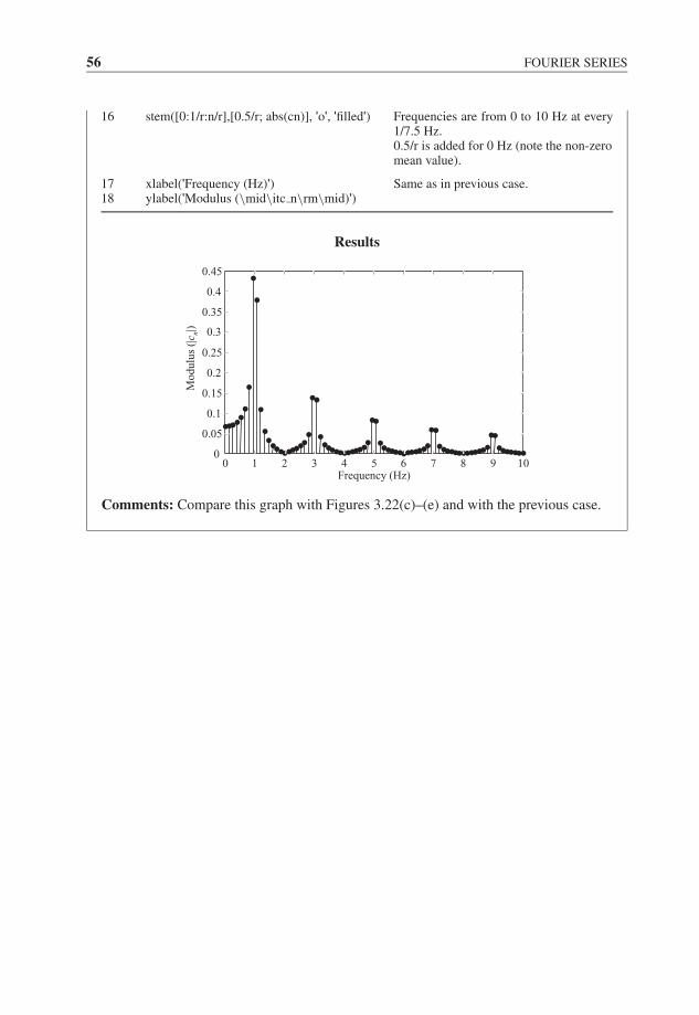
JWBK207-03 JWBK207-Shin January 26, 2008 16:48 Char Count= 0
56 FOURIER SERIES
16 stem([0:1/r:n/r],[0.5/r; abs(cn)], 'o', 'filled') Frequencies are from 0 to 10 Hz at every1/7.5 Hz.0.5/r is added for 0 Hz (note the non-zeromean value).
17 xlabel('Frequency (Hz)') Same as in previous case.18 ylabel('Modulus (\mid\itc n\rm\mid)')
Results
0 1 2 3 4 5 6 7 8 9 100
0.05
0.1
0.15
0.2
0.25
0.3
0.35
0.4
0.45
Frequency (Hz)
Mo
du
lus
(|c n|
)
Comments: Compare this graph with Figures 3.22(c)–(e) and with the previous case.
JWBK207-04 JWBK207-Shin January 18, 2008 9:1 Char Count= 0
4Fourier Integrals (Fourier Transform)and Continuous-Time Linear Systems
Introduction
This chapter introduces the central concept for signal representation, the Fourier integral.All classes of signals may be accommodated from this as a starting point – periodic, almostperiodic, transient and random – though each relies on a rather different perspective andinterpretation.
In addition, the concept of convolution is introduced which allows us to describe linearfiltering and interpret the effect of data truncation (windowing). We begin with a derivationof the Fourier integral.
4.1 THE FOURIER INTEGRAL
We shall extend Fourier analysis to non-periodic phenomena. The basic change in therepresentation is that the discrete summation of the Fourier series becomes a continuoussummation, i.e. an integral form. To demonstrate this change, we begin with the Fourierseries representation of a periodic signal as in Equation (4.1), where the interval ofintegration is defined from −TP/2 to TP/2 for convenience:
x(t) =∞∑
n=−∞cne j2πnt/TP where cn = 1
TP
TP /2∫−TP /2
x(t)e− j2πnt/TP dt (4.1)
As an example, visualize a periodic signal x(t) as having the form below, in Equation(4.2) and Figure 4.1:
x(t) = 0 − TP/2 < t < −1= 1 − 1 < t < 1 (TP/2 > 1)= 0 1 < t < TP/2
(4.2)
Fundamentals of Signal Processing for Sound and Vibration EngineersK. Shin and J. K. Hammond. C© 2008 John Wiley & Sons, Ltd
57
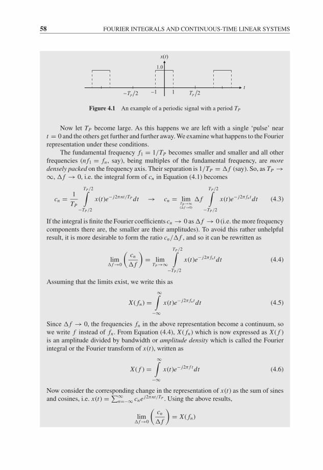
JWBK207-04 JWBK207-Shin January 18, 2008 9:1 Char Count= 0
58 FOURIER INTEGRALS AND CONTINUOUS-TIME LINEAR SYSTEMS
2PT− 2PT11−
1.0
x(t)
t
Figure 4.1 An example of a periodic signal with a period TP
Now let TP become large. As this happens we are left with a single ‘pulse’ neart = 0 and the others get further and further away. We examine what happens to the Fourierrepresentation under these conditions.
The fundamental frequency f1 = 1/TP becomes smaller and smaller and all otherfrequencies (n f1 = fn , say), being multiples of the fundamental frequency, are moredensely packed on the frequency axis. Their separation is 1/TP = � f (say). So, as TP →∞, � f → 0, i.e. the integral form of cn in Equation (4.1) becomes
cn = 1
TP
TP /2∫−TP /2
x(t)e− j2πnt/TP dt → cn = limTP →∞(� f →0)
� f
TP /2∫−TP /2
x(t)e− j2π fn t dt (4.3)
If the integral is finite the Fourier coefficients cn → 0 as � f → 0 (i.e. the more frequencycomponents there are, the smaller are their amplitudes). To avoid this rather unhelpfulresult, it is more desirable to form the ratio cn/� f , and so it can be rewritten as
lim� f →0
(cn
� f
)= lim
TP →∞
TP /2∫−TP /2
x(t)e− j2π fn t dt (4.4)
Assuming that the limits exist, we write this as
X ( fn) =∞∫
−∞x(t)e− j2π fn t dt (4.5)
Since � f → 0, the frequencies fn in the above representation become a continuum, sowe write f instead of fn . From Equation (4.4), X ( fn) which is now expressed as X ( f )is an amplitude divided by bandwidth or amplitude density which is called the Fourierintegral or the Fourier transform of x(t), written as
X ( f ) =∞∫
−∞x(t)e− j2π f t dt (4.6)
Now consider the corresponding change in the representation of x(t) as the sum of sinesand cosines, i.e. x(t) = ∑∞
n=−∞ cne j2πnt/TP . Using the above results,
lim� f →0
(cn
� f
)= X ( fn)
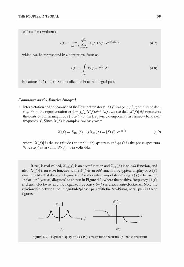
JWBK207-04 JWBK207-Shin January 18, 2008 9:1 Char Count= 0
THE FOURIER INTEGRAL 59
x(t) can be rewritten as
x(t) = lim� f →0
∞∑n=−∞
X ( fn)� f · e j2πnt/TP (4.7)
which can be represented in a continuous form as
x(t) =∞∫
−∞X ( f )e j2π f t d f (4.8)
Equations (4.6) and (4.8) are called the Fourier integral pair.
Comments on the Fourier Integral
1. Interpretation and appearance of the Fourier transform: X ( f ) is a (complex) amplitude den-sity. From the representation x(t) = ∫ ∞
−∞ X ( f )e j2π f t d f , we see that |X ( f )| d f representsthe contribution in magnitude (to x(t)) of the frequency components in a narrow band nearfrequency f . Since X ( f ) is complex, we may write
X ( f ) = XRe( f ) + j X Im( f ) = |X ( f )| e jφ( f ) (4.9)
where |X ( f )| is the magnitude (or amplitude) spectrum and φ( f ) is the phase spectrum.When x(t) is in volts, |X ( f )| is in volts/Hz.
If x(t) is real valued, XRe( f ) is an even function and X Im( f ) is an odd function, andalso |X ( f )| is an even function while φ( f )is an odd function. A typical display of X ( f )may look like that shown in Figure 4.2. An alternative way of displaying X ( f ) is to use the‘polar (or Nyquist) diagram’ as shown in Figure 4.3, where the positive frequency (+ f )is drawn clockwise and the negative frequency (− f ) is drawn anti-clockwise. Note therelationship between the ‘magnitude/phase’ pair with the ‘real/imaginary’ pair in thesefigures.
(b)
( f )φ
f
X( f )
f
(a)
Figure 4.2 Typical display of X ( f ): (a) magnitude spectrum, (b) phase spectrum
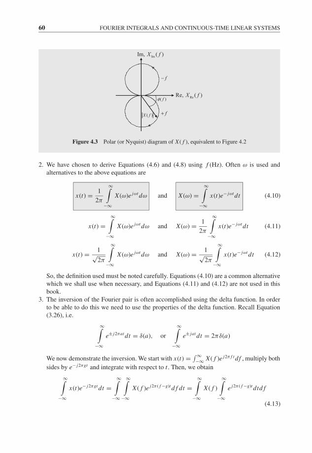
JWBK207-04 JWBK207-Shin January 18, 2008 9:1 Char Count= 0
60 FOURIER INTEGRALS AND CONTINUOUS-TIME LINEAR SYSTEMS
ImIm, ( )X f
ReRe, ( )X f
( )X f
( )fφ
f−
f+
Figure 4.3 Polar (or Nyquist) diagram of X ( f ), equivalent to Figure 4.2
2. We have chosen to derive Equations (4.6) and (4.8) using f (Hz). Often ω is used andalternatives to the above equations are
x(t) = 1
2π
∞∫−∞
X (ω)e jωt dω and X (ω) =∞∫
−∞x(t)e− jωt dt (4.10)
x(t) =∞∫
−∞X (ω)e jωt dω and X (ω) = 1
2π
∞∫−∞
x(t)e− jωt dt (4.11)
x(t) = 1√2π
∞∫−∞
X (ω)e jωt dω and X (ω) = 1√2π
∞∫−∞
x(t)e− jωt dt (4.12)
So, the definition used must be noted carefully. Equations (4.10) are a common alternativewhich we shall use when necessary, and Equations (4.11) and (4.12) are not used in thisbook.
3. The inversion of the Fourier pair is often accomplished using the delta function. In orderto be able to do this we need to use the properties of the delta function. Recall Equation(3.26), i.e.
∞∫−∞
e± j2πat dt = δ(a), or
∞∫−∞
e± jat dt = 2πδ(a)
We now demonstrate the inversion. We start with x(t) = ∫ ∞−∞ X ( f )e j2π f t d f , multiply both
sides by e− j2πgt and integrate with respect to t . Then, we obtain
∞∫−∞
x(t)e− j2πgt dt =∞∫
−∞
∞∫−∞
X ( f )e j2π ( f −g)t d f dt =∞∫
−∞X ( f )
∞∫−∞
e j2π ( f −g)t dtd f
(4.13)
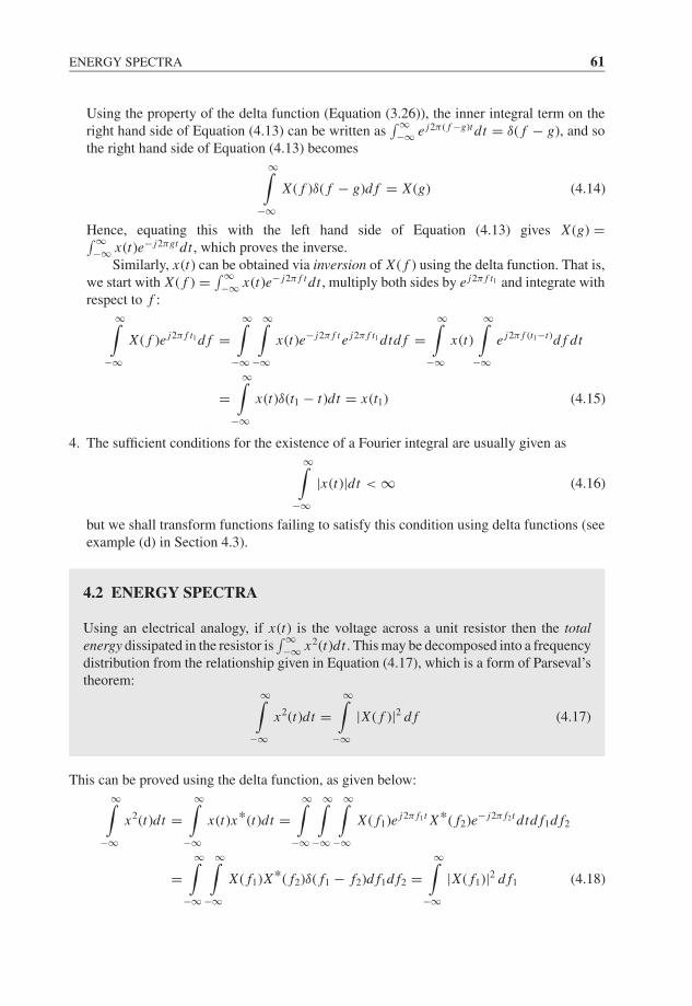
JWBK207-04 JWBK207-Shin January 18, 2008 9:1 Char Count= 0
ENERGY SPECTRA 61
Using the property of the delta function (Equation (3.26)), the inner integral term on theright hand side of Equation (4.13) can be written as
∫ ∞−∞ e j2π ( f −g)t dt = δ( f − g), and so
the right hand side of Equation (4.13) becomes
∞∫−∞
X ( f )δ( f − g)d f = X (g) (4.14)
Hence, equating this with the left hand side of Equation (4.13) gives X (g) =∫ ∞−∞ x(t)e− j2πgt dt , which proves the inverse.
Similarly, x(t) can be obtained via inversion of X ( f ) using the delta function. That is,we start with X ( f ) = ∫ ∞
−∞ x(t)e− j2π f t dt , multiply both sides by e j2π f t1 and integrate withrespect to f :
∞∫−∞
X ( f )e j2π f t1 d f =∞∫
−∞
∞∫−∞
x(t)e− j2π f t e j2π f t1 dtd f =∞∫
−∞x(t)
∞∫−∞
e j2π f (t1−t)d f dt
=∞∫
−∞x(t)δ(t1 − t)dt = x(t1) (4.15)
4. The sufficient conditions for the existence of a Fourier integral are usually given as
∞∫−∞
|x(t)|dt < ∞ (4.16)
but we shall transform functions failing to satisfy this condition using delta functions (seeexample (d) in Section 4.3).
4.2 ENERGY SPECTRA
Using an electrical analogy, if x(t) is the voltage across a unit resistor then the totalenergy dissipated in the resistor is
∫ ∞−∞ x2(t)dt . This may be decomposed into a frequency
distribution from the relationship given in Equation (4.17), which is a form of Parseval’stheorem:
∞∫−∞
x2(t)dt =∞∫
−∞|X ( f )|2 d f (4.17)
This can be proved using the delta function, as given below:
∞∫−∞
x2(t)dt =∞∫
−∞x(t)x*(t)dt =
∞∫−∞
∞∫−∞
∞∫−∞
X ( f1)e j2π f1t X*( f2)e− j2π f2t dtd f1d f2
=∞∫
−∞
∞∫−∞
X ( f1)X*( f2)δ( f1 − f2)d f1d f2 =∞∫
−∞|X ( f1)|2 d f1 (4.18)
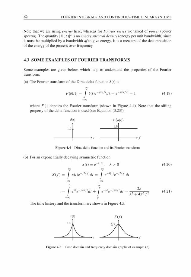
JWBK207-04 JWBK207-Shin January 18, 2008 9:1 Char Count= 0
62 FOURIER INTEGRALS AND CONTINUOUS-TIME LINEAR SYSTEMS
Note that we are using energy here, whereas for Fourier series we talked of power (powerspectra). The quantity |X ( f )|2 is an energy spectral density (energy per unit bandwidth) sinceit must be multiplied by a bandwidth df to give energy. It is a measure of the decompositionof the energy of the process over frequency.
4.3 SOME EXAMPLES OF FOURIER TRANSFORMS
Some examples are given below, which help to understand the properties of the Fouriertransform:
(a) The Fourier transform of the Dirac delta function δ(t) is
F{δ(t)} =∞∫
−∞δ(t)e− j2π f t dt = e− j2π f ·0 = 1 (4.19)
where F{} denotes the Fourier transform (shown in Figure 4.4). Note that the siftingproperty of the delta function is used (see Equation (3.23)).
( )tδ
1.0
t
1.0
{ }( )F tδ
f
Figure 4.4 Dirac delta function and its Fourier transform
(b) For an exponentially decaying symmetric function
x(t) = e−λ| t |, λ > 0 (4.20)
X ( f ) =∞∫
−∞x(t)e− j2π f t dt =
∞∫−∞
e−λ| t |e− j2π f t dt
=0∫
−∞eλt e− j2π f t dt +
∞∫0
e−λt e− j2π f t dt = 2λ
λ2 + 4π2 f 2(4.21)
The time history and the transform are shown in Figure 4.5.
( )x t
1.0
t
( )X f
2 λ
f
Figure 4.5 Time domain and frequency domain graphs of example (b)
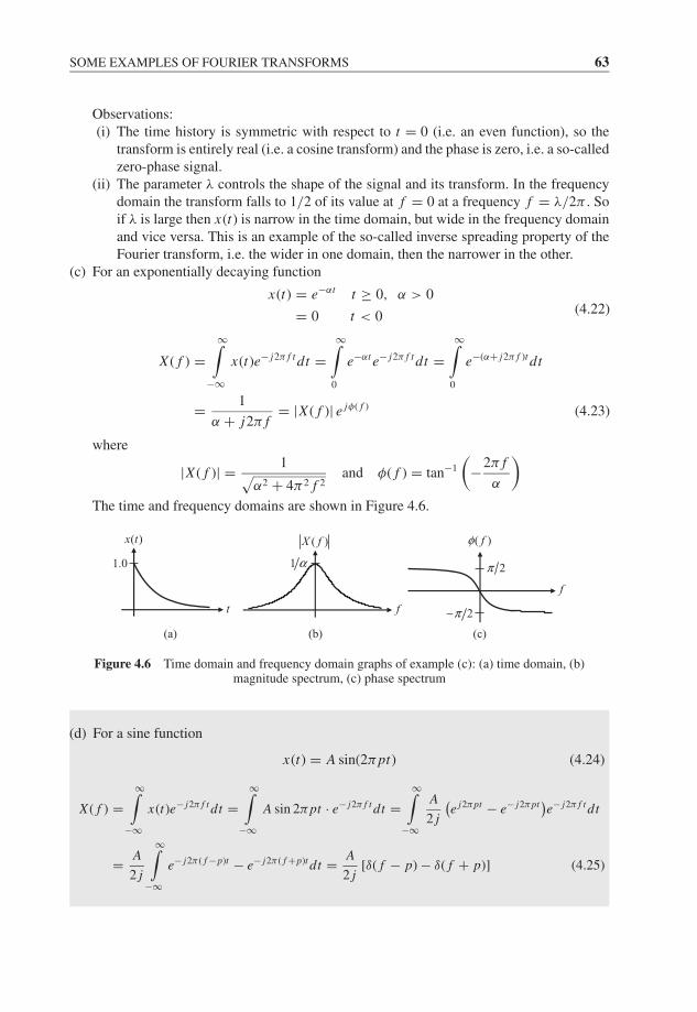
JWBK207-04 JWBK207-Shin January 18, 2008 9:1 Char Count= 0
SOME EXAMPLES OF FOURIER TRANSFORMS 63
Observations:(i) The time history is symmetric with respect to t = 0 (i.e. an even function), so the
transform is entirely real (i.e. a cosine transform) and the phase is zero, i.e. a so-calledzero-phase signal.
(ii) The parameter λ controls the shape of the signal and its transform. In the frequencydomain the transform falls to 1/2 of its value at f = 0 at a frequency f = λ/2π . Soif λ is large then x(t) is narrow in the time domain, but wide in the frequency domainand vice versa. This is an example of the so-called inverse spreading property of theFourier transform, i.e. the wider in one domain, then the narrower in the other.
(c) For an exponentially decaying function
x(t) = e−αt t ≥ 0, α > 0
= 0 t < 0(4.22)
X ( f ) =∞∫
−∞x(t)e− j2π f t dt =
∞∫0
e−αt e− j2π f t dt =∞∫
0
e−(α+ j2π f )t dt
= 1
α + j2π f= |X ( f )| e jφ( f ) (4.23)
where
|X ( f )| = 1√α2 + 4π2 f 2
and φ( f ) = tan−1
(−2π f
α
)The time and frequency domains are shown in Figure 4.6.
(a) (b) (c)
( )X f
1 α
f
2π
2π−
( )fφ
f
( )x t
t
1.0
Figure 4.6 Time domain and frequency domain graphs of example (c): (a) time domain, (b)magnitude spectrum, (c) phase spectrum
(d) For a sine function
x(t) = A sin(2πpt) (4.24)
X ( f ) =∞∫
−∞x(t)e− j2π f t dt =
∞∫−∞
A sin 2πpt · e− j2π f t dt =∞∫
−∞
A
2 j
(e j2πpt − e− j2πpt
)e− j2π f t dt
= A
2 j
∞∫−∞
e− j2π ( f −p)t − e− j2π ( f +p)t dt = A
2 j[δ( f − p) − δ( f + p)] (4.25)

JWBK207-04 JWBK207-Shin January 18, 2008 9:1 Char Count= 0
64 FOURIER INTEGRALS AND CONTINUOUS-TIME LINEAR SYSTEMS
1 p
x(t)
A
t2A
p− p
2A
X( f )
f
Figure 4.7 Time domain and frequency domain graphs of example (d)
In this example, X ( f ) is non-zero at f = p and f = −p only, and is imaginary valued(the sine function is an odd function). The phase components are arg X (p) = −π/2 andarg X (−p) = π/2. This shows that a distinct frequency component results in spikes inthe amplitude density.
(e) For a rectangular pulse
x(t) = a | t | < b(4.26)
= 0 | t | > b
X ( f ) =∞∫
−∞x(t)e− j2π f t dt =
b∫−b
ae− j2π f t dt
= 2ab sin(2π f b)
2π f b(4.27)
a
tb− b
1
2b
1
b
3
2b
X( f )x(t)
2ab
f
Figure 4.8 Time domain and frequency domain graphs of example (e)
The expression for X ( f ) has been written so as to highlight the term sin(2π f b)/2π f b,i.e. sin(x)/x , which is the so-called sinc function which is unity at x = 0, and thereafteris an amplitude-modulated oscillation, where the modulation is 1/x . The width (in time)of x(t) is 2b and the distance to the first zero crossing in the frequency domain is 1/2b(as shown in Figure 4.8). This once again demonstrates the inverse spreading property.
For the case a = 1, then as b → ∞, X ( f ) is more and more concentrated aroundf = 0 and becomes taller and taller. In fact, limb→∞ 2b sin(2π f b)/2π f b is another wayof expressing the delta function δ( f ), as we have seen in Chapter 3 (see Equation (3.27)).
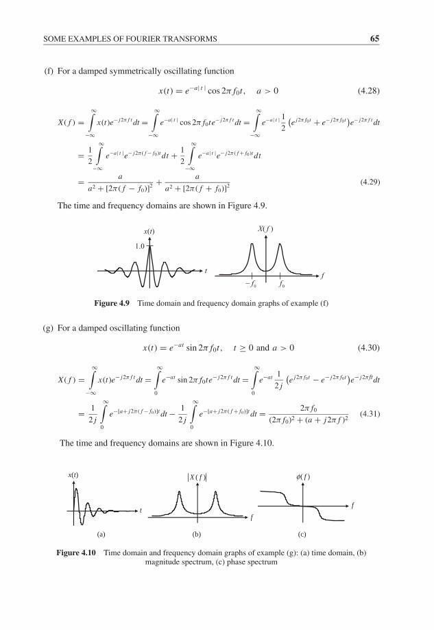
JWBK207-04 JWBK207-Shin January 18, 2008 9:1 Char Count= 0
SOME EXAMPLES OF FOURIER TRANSFORMS 65
(f) For a damped symmetrically oscillating function
x(t) = e−a| t | cos 2π f0t, a > 0 (4.28)
X ( f ) =∞∫
−∞
x(t)e− j2π f t dt =∞∫
−∞
e−a| t | cos 2π f0te− j2π f t dt =∞∫
−∞
e−a| t | 1
2
(e j2π f0t + e− j2π f0t
)e− j2π f t dt
= 1
2
∞∫−∞
e−a| t |e− j2π ( f − f0)t dt + 1
2
∞∫−∞
e−a| t |e− j2π ( f + f0)t dt
= a
a2 + [2π ( f − f0)]2+ a
a2 + [2π ( f + f0)]2(4.29)
The time and frequency domains are shown in Figure 4.9.
x(t)
1.0
t
X( f )
f0f− 0f
Figure 4.9 Time domain and frequency domain graphs of example (f)
(g) For a damped oscillating function
x(t) = e−at sin 2π f0t, t ≥ 0 and a > 0 (4.30)
X ( f ) =∞∫
−∞x(t)e− j2π f t dt =
∞∫0
e−at sin 2π f0te− j2π f t dt =∞∫
0
e−at 1
2 j
(e j2π f0t − e− j2π f0t
)e− j2π ftdt
= 1
2 j
∞∫0
e−[a+ j2π ( f − f0)]t dt − 1
2 j
∞∫0
e−[a+ j2π ( f + f0)]t dt = 2π f0
(2π f0)2 + (a + j2π f )2(4.31)
The time and frequency domains are shown in Figure 4.10.
(a) (b) (c)
x(t)
tf
( )X f
f
( f )φ
Figure 4.10 Time domain and frequency domain graphs of example (g): (a) time domain, (b)magnitude spectrum, (c) phase spectrum

JWBK207-04 JWBK207-Shin January 18, 2008 9:1 Char Count= 0
66 FOURIER INTEGRALS AND CONTINUOUS-TIME LINEAR SYSTEMS
(h) For the Gaussian pulse
x(t) = e−at2
, a > 0 (4.32)
X (ω) =√
π/a · e−ω2/4a (4.33)
i.e. X (ω) is also a Gaussian pulse. Proof of Equation (4.33) is given below. We shall useX (ω) instead of X ( f ) for convenience.
We start from
X (ω) =∞∫
−∞e−at2
e− jωt dt =∞∫
−∞e−a(t2+ jωt/a)dt
and multiply by e−ω2/4a · eω2/4a to complete the square, i.e. so that
X (ω) = e−ω2/4a ·∞∫
−∞e−a(t2+ jωt/a−ω2/4a2)dt = e−ω2/4a ·
∞∫−∞
e−a[t+ j(ω/2a)]2
dt
Now, let y = [t + j(ω/2a)]; then finally we have
X (ω) = e−ω2/4a ·∞∫
−∞e−ay2
dy =√
π/a · e−ω2/4a
The time and frequency domains are shown in Figure 4.11.
x(t)
1.0
t
aπ
( )X ω
ω
Figure 4.11 Time domain and frequency domain graphs of example (h)
(i) For a unit step function
u(t) = 1 t > 0
= 0 t < 0 (4.34)
The unit step function is not defined at t = 0, i.e. it has a discontinuity at this point. TheFourier transform of u(t) is given by
F{u(t)} = 1
2δ( f ) + 1
j2π f(4.35)
where F{} denotes the Fourier transform (shown in Figure 4.12). The derivation of thisresult requires the use of the delta function and some properties of the Fourier transform.Details of the derivation can be found in Hsu (1970), if required. Also, note the presenceof the delta function at f = 0, which indicates a d.c. component.
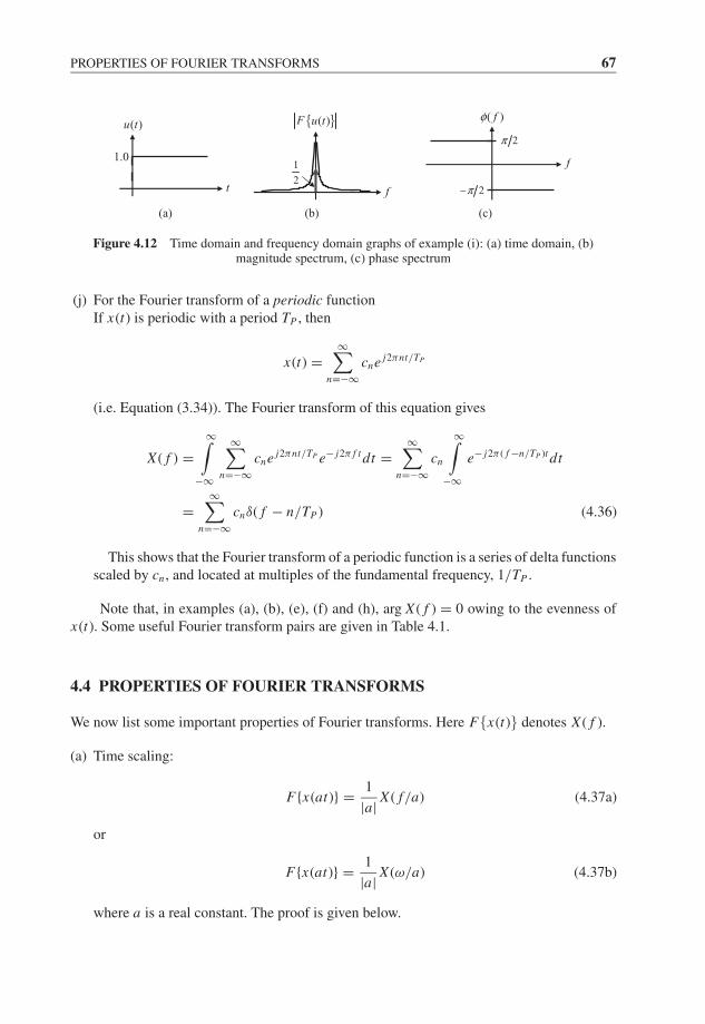
JWBK207-04 JWBK207-Shin January 18, 2008 9:1 Char Count= 0
PROPERTIES OF FOURIER TRANSFORMS 67
(a) (b) (c)
( )u t
1.0
t
1
2
{ }( )F u t
f
2π
( )fφ
2π−
f
Figure 4.12 Time domain and frequency domain graphs of example (i): (a) time domain, (b)magnitude spectrum, (c) phase spectrum
(j) For the Fourier transform of a periodic functionIf x(t) is periodic with a period TP , then
x(t) =∞∑
n=−∞cne j2πnt/TP
(i.e. Equation (3.34)). The Fourier transform of this equation gives
X ( f ) =∞∫
−∞
∞∑n=−∞
cne j2πnt/TP e− j2π f t dt =∞∑
n=−∞cn
∞∫−∞
e− j2π ( f −n/TP )t dt
=∞∑
n=−∞cnδ( f − n/TP ) (4.36)
This shows that the Fourier transform of a periodic function is a series of delta functionsscaled by cn , and located at multiples of the fundamental frequency, 1/TP .
Note that, in examples (a), (b), (e), (f) and (h), arg X ( f ) = 0 owing to the evenness ofx(t). Some useful Fourier transform pairs are given in Table 4.1.
4.4 PROPERTIES OF FOURIER TRANSFORMS
We now list some important properties of Fourier transforms. Here F{x(t)} denotes X ( f ).
(a) Time scaling:
F{x(at)} = 1
|a| X ( f/a) (4.37a)
or
F{x(at)} = 1
|a| X (ω/a) (4.37b)
where a is a real constant. The proof is given below.
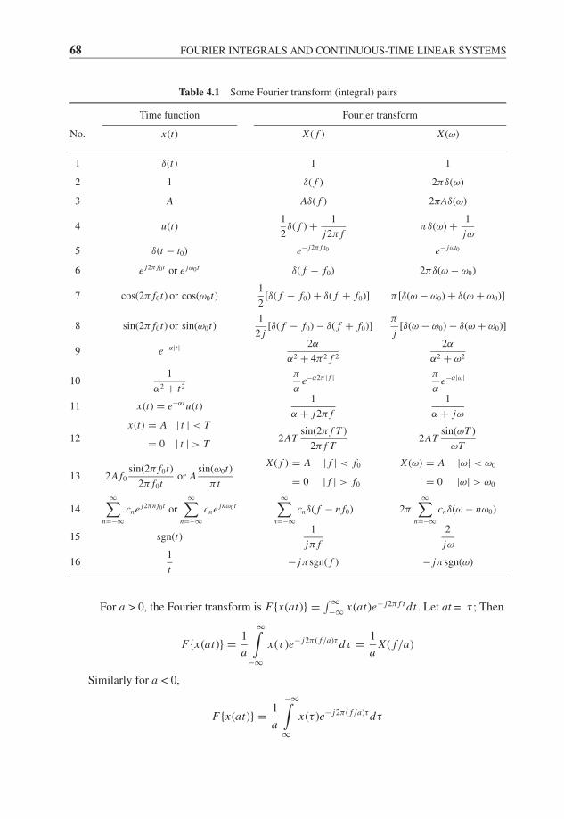
JWBK207-04 JWBK207-Shin January 18, 2008 9:1 Char Count= 0
68 FOURIER INTEGRALS AND CONTINUOUS-TIME LINEAR SYSTEMS
Table 4.1 Some Fourier transform (integral) pairs
Time function Fourier transform
No. x(t) X ( f ) X (ω)
1 δ(t) 1 1
2 1 δ( f ) 2πδ(ω)
3 A Aδ( f ) 2πAδ(ω)
4 u(t)1
2δ( f ) + 1
j2π fπδ(ω) + 1
jω
5 δ(t − t0) e− j2π f t0 e− jωt0
6 e j2π f0t or e jω0t δ( f − f0) 2πδ(ω − ω0)
7 cos(2π f0t) or cos(ω0t)1
2[δ( f − f0) + δ( f + f0)] π [δ(ω − ω0) + δ(ω + ω0)]
8 sin(2π f0t) or sin(ω0t)1
2 j[δ( f − f0) − δ( f + f0)]
π
j[δ(ω − ω0) − δ(ω + ω0)]
9 e−α|t | 2α
α2 + 4π 2 f 2
2α
α2 + ω2
101
α2 + t2
π
αe−α2π | f | π
αe−α|ω|
11 x(t) = e−αt u(t)1
α + j2π f
1
α + jω
12
x(t) = A | t | < T
= 0 | t | > T 2ATsin(2π f T )
2π f T2AT
sin(ωT )
ωT
13 2A f0
sin(2π f0t)
2π f0tor A
sin(ω0t)
π t
X ( f ) = A | f | < f0
= 0 | f | > f0
X (ω) = A |ω| < ω0
= 0 |ω| > ω0
14∞∑
n=−∞cne j2πn f0t or
∞∑n=−∞
cne jnω0t∞∑
n=−∞cnδ( f − n f0) 2π
∞∑n=−∞
cnδ(ω − nω0)
15 sgn(t)1
jπ f
2
jω
161
t− jπsgn( f ) − jπsgn(ω)
For a > 0, the Fourier transform is F{x(at)} = ∫ ∞−∞ x(at)e− j2π f t dt . Let at = τ ; Then
F{x(at)} = 1
a
∞∫−∞
x(τ )e− j2π ( f/a)τ dτ = 1
aX ( f/a)
Similarly for a < 0,
F{x(at)} = 1
a
−∞∫∞
x(τ )e− j2π ( f/a)τ dτ

JWBK207-04 JWBK207-Shin January 18, 2008 9:1 Char Count= 0
PROPERTIES OF FOURIER TRANSFORMS 69
thus
F{x(at)} = −1
a
∞∫−∞
x(τ )e− j2π ( f/a)τ dτ = 1
|a| X ( f/a)
That is, time scaling results in frequency scaling, again demonstrating the inverse spreadingrelationship.
(b) Time reversal:
F{x(−t)} = X (− f ) (= X∗( f ), for x(t) real) (4.38a)
or
F{x(−t)} = X (−ω) (4.38b)
Proof: We start from F{x(−t)} = ∫ ∞−∞ x(−t)e− j2π f t dt , let −t = τ , then obtain
F{x(−t)} = −−∞∫∞
x(τ )e j2π f τ dτ =∞∫
−∞x(τ )e− j2π (− f )τ dτ = X (− f )
Note that if x(t) is real, then x∗(t) = x(t). In this case,
X (− f ) =∞∫
−∞x(t)e− j2π (− f )t dt =
∞∫−∞
x∗(t)e j2π f t dt = X∗( f )
This is called the conjugate symmetry property.It is interesting to note that the Fourier transform of X (−ω) is x(t), i.e. F{X (−ω)} =
x(t), and similarly F{X (ω)} = x(−t).(c) Time shifting:
F{x(t − t0)} = e− j2π f t0 X ( f ) (4.39a)
or
F{x(t − t0)} = e− jωt0 X (ω) (4.39b)
Proof: We start from F{x(t − t0)} = ∫ ∞−∞ x(t − t0)e− j2π f t dt , let t − t0 = τ , then obtain
F{x(t − t0)} =∞∫
−∞x(τ )e− j2π f (t0+τ )dτ = e− j2π f t0
∞∫−∞
x(τ )e− j2π f τ dτ = e− j2π f t0 X ( f )
This important property is expanded upon in Section 4.5.(d) Modulation (or multiplication) property:
(i) F{
x(t)e j2π f0t} = X ( f − f0) (4.40a)
or
F{
x(t)e jω0t} = X (ω − ω0) (4.40b)
This property is usually known as the ‘frequency shifting’ property.
JWBK207-04 JWBK207-Shin January 18, 2008 9:1 Char Count= 0
70 FOURIER INTEGRALS AND CONTINUOUS-TIME LINEAR SYSTEMS
Proof:
F{
x(t)e j2π f0t} =
∞∫−∞
x(t)e j2π f0t e− j2π f t dt =∞∫
−∞x(t)e− j2π ( f − f0)t dt = X ( f − f0)
(ii)F{x(t) cos(2π f0t)} = 1
2[X ( f − f0) + X ( f + f0)] (4.41a)
or
F{x(t) cos(ω0t)} = 1
2[X (ω − ω0) + X (ω + ω0)] (4.41b)
This characterizes ‘amplitude modulation’. For communication systems, usually x(t)is a low-frequency signal, and cos(2π f0t) is a high-frequency carrier signal.
Proof:
F{x(t) cos(2π f0t)} = F
{1
2x(t)e j2π f0t + 1
2x(t)e− j2π f0t
}= 1
2F
{x(t)e j2π f0t
} +1
2F
{x(t)e− j2π f0t
}= 1
2[X ( f − f0) + X ( f + f0)]
(e) Differentiation:
F{x(t)} = j2π f X ( f ) (if x(t) → 0 as t → ±∞) (4.42a)
or
F{x(t)} = jωX (ω) (4.42b)
Proof:
F{x(t)} =∞∫
−∞x(t)e− j2π f t dt = x(t)e− j2π f t
∣∣∞−∞ + j2π f
∞∫−∞
x(t)e− j2π f t dt
Since x(t) → 0 as t → ±∞, the first part of the right hand side diminishes. Thus
F{x(t)} = j2π f
∞∫−∞
x(t)e− j2π f t dt = j2π f X ( f )
(f) The Fourier transform of the ‘convolution’ of two functions:
F{h(t) ∗ x(t)} = H ( f )X ( f ) (4.43)
where the convolution of the two functions h(t) and x(t) is defined as
h(t) ∗ x(t) =∞∫
−∞h(τ )x(t − τ )dτ (4.44)
JWBK207-04 JWBK207-Shin January 18, 2008 9:1 Char Count= 0
THE IMPORTANCE OF PHASE 71
The property of Equation (4.43) is very important in linear system theory and is explainedfully in Section 4.7.
Proof: Let t − τ = v. Then
F{h(t) ∗ x(t)} =∞∫
−∞
∞∫−∞
h(τ )x(t − τ )e− j2π f t dτdt
=∞∫
−∞
∞∫−∞
h(τ )x(v)e− j2π f (τ+v)dτdv
=∞∫
−∞h(τ )e− j2π f τ dτ
∞∫−∞
x(v)e− j2π f vdv = H ( f )X ( f )
(g) The Fourier transform of the ‘product’ of two functions:
F{x(t)w(t)} =∞∫
−∞X (g)W ( f − g)dg = X ( f ) ∗ W ( f ) (4.45)
This is also a very important property, and will be examined in detail in Section 4.11.
Proof: We start from F{x(t)w(t)} = ∫ ∞−∞ x(t)w(t)e− j2π f t dt . If x(t) and w(t) both have
Fourier representations, then the right hand side is
∞∫−∞
x(t)w(t)e− j2π f t dt =∞∫
−∞
∞∫−∞
∞∫−∞
X ( f1)e j2π f1t W ( f2)e j2π f2t · e− j2π f t d f1d f2dt
=∞∫
−∞X ( f1)
∞∫−∞
W ( f2)
∞∫−∞
e− j2π ( f − f1− f2)t dtd f2d f1
=∞∫
−∞X ( f1)
∞∫−∞
W ( f2)δ( f − f1 − f2)d f2d f1
=∞∫
−∞X ( f1)W ( f − f1)d f1 = X ( f ) ∗ W ( f )
4.5 THE IMPORTANCE OF PHASE
In many cases, we sometimes only draw the magnitude spectral density, |X ( f )|, andnot the phase spectral density, arg X ( f ) = φ( f ). However, in order to reconstruct asignal we need both. An infinite number of different-looking signals may have the same
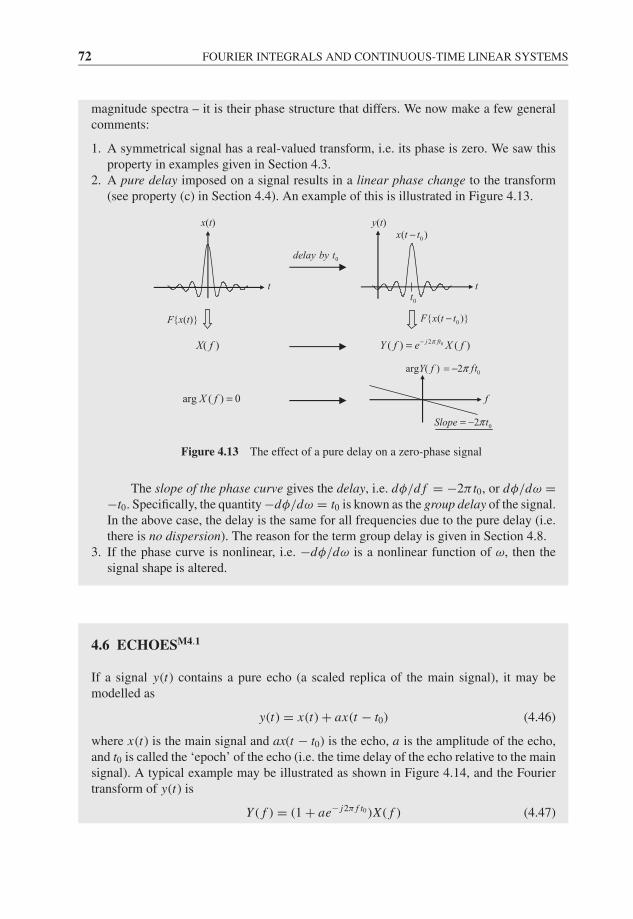
JWBK207-04 JWBK207-Shin January 18, 2008 9:1 Char Count= 0
72 FOURIER INTEGRALS AND CONTINUOUS-TIME LINEAR SYSTEMS
magnitude spectra – it is their phase structure that differs. We now make a few generalcomments:
1. A symmetrical signal has a real-valued transform, i.e. its phase is zero. We saw thisproperty in examples given in Section 4.3.
2. A pure delay imposed on a signal results in a linear phase change to the transform(see property (c) in Section 4.4). An example of this is illustrated in Figure 4.13.
X( f ) 02( ) ( )j ftY f e X fπ−=
arg ( ) 0X f =
F{x(t)} 0{ ( )}F x t t−
02Slope tπ−=
02argY( f ) f tπ−=
y(t)
0( )x t t−
0tt
x(t)
t
0delay by t
f
Figure 4.13 The effect of a pure delay on a zero-phase signal
The slope of the phase curve gives the delay, i.e. dφ/d f = −2π t0, or dφ/dω =−t0. Specifically, the quantity −dφ/dω = t0 is known as the group delay of the signal.In the above case, the delay is the same for all frequencies due to the pure delay (i.e.there is no dispersion). The reason for the term group delay is given in Section 4.8.
3. If the phase curve is nonlinear, i.e. −dφ/dω is a nonlinear function of ω, then thesignal shape is altered.
4.6 ECHOESM4.1
If a signal y(t) contains a pure echo (a scaled replica of the main signal), it may bemodelled as
y(t) = x(t) + ax(t − t0) (4.46)
where x(t) is the main signal and ax(t − t0) is the echo, a is the amplitude of the echo,and t0 is called the ‘epoch’ of the echo (i.e. the time delay of the echo relative to the mainsignal). A typical example may be illustrated as shown in Figure 4.14, and the Fouriertransform of y(t) is
Y ( f ) = (1 + ae− j2π f t0 )X ( f ) (4.47)
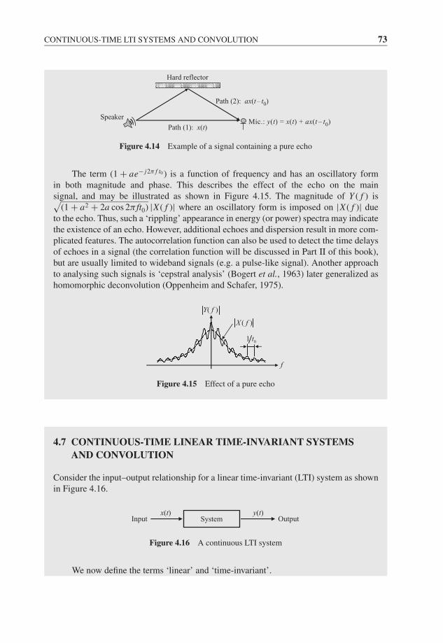
JWBK207-04 JWBK207-Shin January 18, 2008 9:1 Char Count= 0
CONTINUOUS-TIME LTI SYSTEMS AND CONVOLUTION 73
Mic.: y(t) = x(t) + ax(t – t0)
Hard reflector
Speaker
Path (1): x(t)
Path (2): ax(t – t0)
Figure 4.14 Example of a signal containing a pure echo
The term (1 + ae− j2π f t0 ) is a function of frequency and has an oscillatory formin both magnitude and phase. This describes the effect of the echo on the mainsignal, and may be illustrated as shown in Figure 4.15. The magnitude of Y ( f ) is√
(1 + a2 + 2a cos 2π ft0) |X ( f )| where an oscillatory form is imposed on |X ( f )| dueto the echo. Thus, such a ‘rippling’ appearance in energy (or power) spectra may indicatethe existence of an echo. However, additional echoes and dispersion result in more com-plicated features. The autocorrelation function can also be used to detect the time delaysof echoes in a signal (the correlation function will be discussed in Part II of this book),but are usually limited to wideband signals (e.g. a pulse-like signal). Another approachto analysing such signals is ‘cepstral analysis’ (Bogert et al., 1963) later generalized ashomomorphic deconvolution (Oppenheim and Schafer, 1975).
01 t
Y( f )
X ( f )
f
Figure 4.15 Effect of a pure echo
4.7 CONTINUOUS-TIME LINEAR TIME-INVARIANT SYSTEMSAND CONVOLUTION
Consider the input–output relationship for a linear time-invariant (LTI) system as shownin Figure 4.16.
Systemy(t)x(t)
OutputInput
Figure 4.16 A continuous LTI system
We now define the terms ‘linear’ and ‘time-invariant’.

JWBK207-04 JWBK207-Shin January 18, 2008 9:1 Char Count= 0
74 FOURIER INTEGRALS AND CONTINUOUS-TIME LINEAR SYSTEMS
Linearity
Let y1(t) and y2(t) be the responses of the system to inputs x1(t) and x2(t), respectively.If the system is linear it satisfies the properties in Figure 4.17, where a is an arbitraryconstant.
Linear system(i) Additivity: x1(t) + x2(t)
ax1(t)
y1(t) + y2(t)
ay1(t)(ii) Scaling (or homogeneity): Linear system
Figure 4.17 Properties of a linear system
Or the two properties can be combined to give a more general expression thatis known as the ‘superposition property’ (Figure 4.18), where a1 and a2 are arbitraryconstants.
Linear system1 1 2 2( ) ( )a x t a x t+ 1 1 2 2( ) ( )a y t a y t+
Figure 4.18 Superposition property of a linear system
Time Invariance
A time-invariant system may be illustrated as in Figure 4.19, such that if the input isshifted by t0, then the response will also be shifted by the same amount of time.
Time-invariant systemx(t − t0) y(t − t
0)
Figure 4.19 Property of a time-invariant system
Mathematical Characterization of an LTI System
Very commonly LTI systems are described in differential equation form. The forced vibra-tion of a single-degree-of-freedom system is a typical example, which may be expressedas
my(t) + cy(t) + ky(t) = x(t) (4.48)
where x(t) is the input and y(t) is the output of the system.Relating y(t) to x(t) in the time domain then requires the solution of the differential
equation. Transformation (Laplace and Fourier) techniques allow a ‘systems approach’with the input/response relationships described by transfer functions or frequency re-sponse functions.
We shall use a general approach to linear system characterization that does notrequire a differential equation format. We could characterize a system in terms of itsresponse to specific inputs, e.g. a step input or a harmonic input, but we shall find thatthe response to an ideal impulse (the Dirac delta function) turns out to be very helpful -even though such an input is a mathematical idealization.
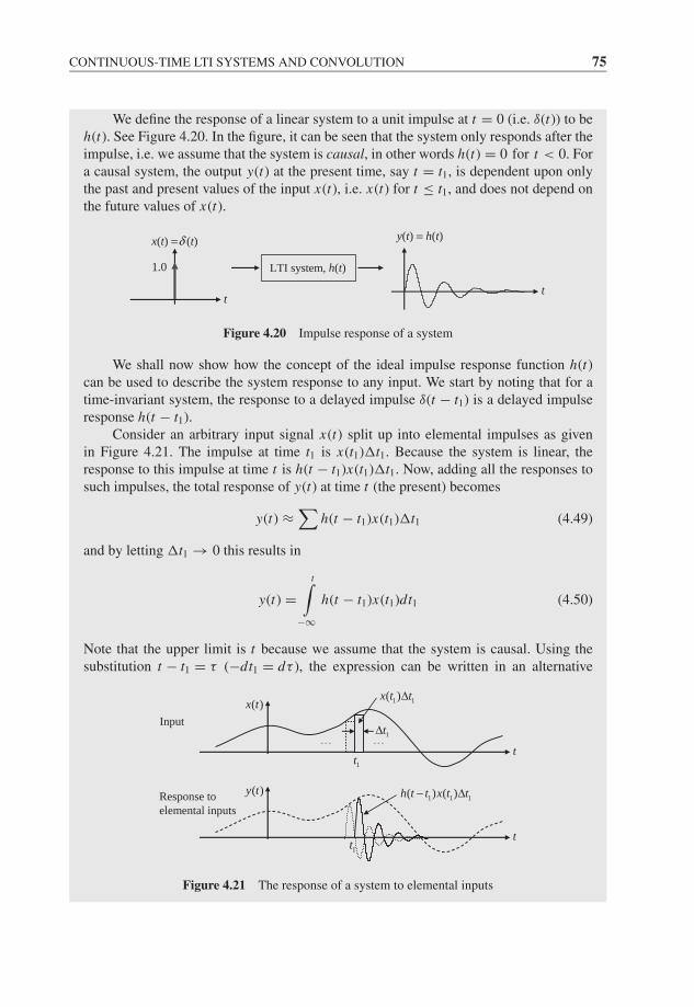
JWBK207-04 JWBK207-Shin January 18, 2008 9:1 Char Count= 0
CONTINUOUS-TIME LTI SYSTEMS AND CONVOLUTION 75
We define the response of a linear system to a unit impulse at t = 0 (i.e. δ(t)) to beh(t). See Figure 4.20. In the figure, it can be seen that the system only responds after theimpulse, i.e. we assume that the system is causal, in other words h(t) = 0 for t < 0. Fora causal system, the output y(t) at the present time, say t = t1, is dependent upon onlythe past and present values of the input x(t), i.e. x(t) for t ≤ t1, and does not depend onthe future values of x(t).
LTI system, h(t)
δx(t) = (t)
1.0
t
y(t) = h(t)
t
Figure 4.20 Impulse response of a system
We shall now show how the concept of the ideal impulse response function h(t)can be used to describe the system response to any input. We start by noting that for atime-invariant system, the response to a delayed impulse δ(t − t1) is a delayed impulseresponse h(t − t1).
Consider an arbitrary input signal x(t) split up into elemental impulses as givenin Figure 4.21. The impulse at time t1 is x(t1)�t1. Because the system is linear, theresponse to this impulse at time t is h(t − t1)x(t1)�t1. Now, adding all the responses tosuch impulses, the total response of y(t) at time t (the present) becomes
y(t) ≈∑
h(t − t1)x(t1)�t1 (4.49)
and by letting �t1 → 0 this results in
y(t) =t∫
−∞h(t − t1)x(t1)dt1 (4.50)
Note that the upper limit is t because we assume that the system is causal. Using thesubstitution t − t1 = τ (−dt1 = dτ ), the expression can be written in an alternative
…Input
Response to elemental inputs
1 1( )x t tΔ
1tΔ
1 1 1( ) ( )h t t x t t− Δ
1t
1t
…
( )x t
( )y t
t
t
Figure 4.21 The response of a system to elemental inputs
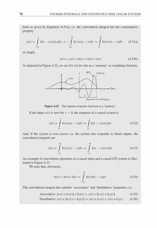
JWBK207-04 JWBK207-Shin January 18, 2008 9:1 Char Count= 0
76 FOURIER INTEGRALS AND CONTINUOUS-TIME LINEAR SYSTEMS
form as given by Equation (4.51a), i.e. the convolution integral has the commutativeproperty
y(t) =t∫
−∞h(t − t1)x(t1)dt1 = −
0∫∞
h(τ )x(t − τ )dτ =∞∫
0
h(τ )x(t − τ )dτ (4.51a)
or simply
y(t) = x(t) ∗ h(t) = h(t) ∗ x(t) (4.51b)
As depicted in Figure 4.22, we see h(τ ) in its role as a ‘memory’ or weighting function.
h(τ) t (Now)
τ
1t
x(t)
Time
Past Future
Figure 4.22 The impulse response function as a ‘memory’
If the input x(t) is zero for t < 0, the response of a causal system is
y(t) =t∫
0
h(τ )x(t − τ )dτ =t∫
0
h(t − τ )x(τ )dτ (4.52)
And, if the system is non-causal, i.e. the system also responds to future inputs, theconvolution integrals are
y(t) =∞∫
−∞h(τ )x(t − τ )dτ =
∞∫−∞
h(t − τ )x(τ )dτ (4.53)
An example of convolution operation of a causal input and a causal LTI system is illus-trated in Figure 4.23.
We note that, obviously,
h(t) = h(t) ∗ δ(t) =∞∫
−∞h(τ )δ(t − τ )dτ (4.54)
The convolution integral also satisfies ‘associative’ and ‘distributive’ properties, i.e.
Associative: [x(t) ∗ h1(t)] ∗ h2(t) = x(t) ∗ [h1(t) ∗ h2(t)] (4.55)
Distributive: x(t) ∗ [h1(t) + h2(t)] = x(t) ∗ h1(t) + x(t) ∗ h2(t) (4.56)
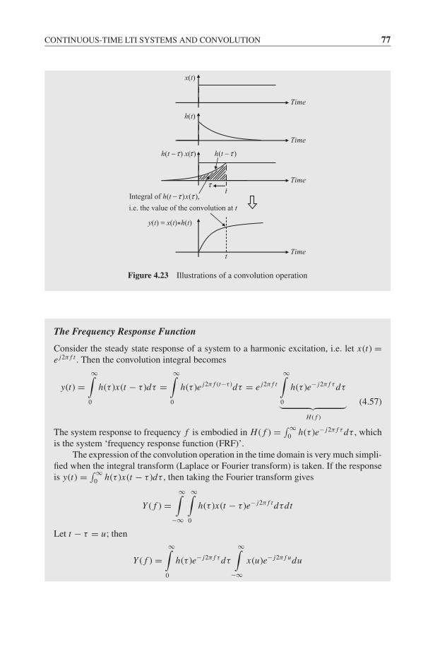
JWBK207-04 JWBK207-Shin January 18, 2008 9:1 Char Count= 0
CONTINUOUS-TIME LTI SYSTEMS AND CONVOLUTION 77
Integral of ( ) ( ),
i.e. the value of the convolution at t
h t xτ τ−
Time
h(t)
x(t)
Time
τ τ
Time
( )h t τ−
tτ
y(t) = x(t)*h(t)
h(t − ) x( )
tTime
Figure 4.23 Illustrations of a convolution operation
The Frequency Response Function
Consider the steady state response of a system to a harmonic excitation, i.e. let x(t) =e j2π f t . Then the convolution integral becomes
y(t) =∞∫
0
h(τ )x(t − τ )dτ =∞∫
0
h(τ )e j2π f (t−τ )dτ = e j2π f t
∞∫0
h(τ )e− j2π f τ dτ
︸ ︷︷ ︸H ( f )
(4.57)
The system response to frequency f is embodied in H ( f ) = ∫ ∞0
h(τ )e− j2π f τ dτ , whichis the system ‘frequency response function (FRF)’.
The expression of the convolution operation in the time domain is very much simpli-fied when the integral transform (Laplace or Fourier transform) is taken. If the responseis y(t) = ∫ ∞
0h(τ )x(t − τ )dτ , then taking the Fourier transform gives
Y ( f ) =∞∫
−∞
∞∫0
h(τ )x(t − τ )e− j2π f t dτdt
Let t − τ = u; then
Y ( f ) =∞∫
0
h(τ )e− j2π f τ dτ
∞∫−∞
x(u)e− j2π f udu
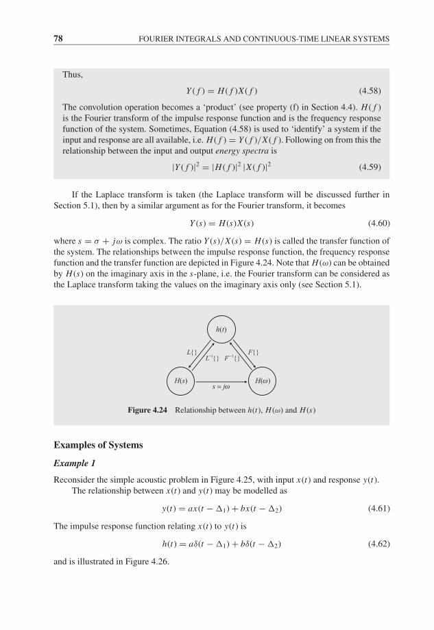
JWBK207-04 JWBK207-Shin January 18, 2008 9:1 Char Count= 0
78 FOURIER INTEGRALS AND CONTINUOUS-TIME LINEAR SYSTEMS
Thus,
Y ( f ) = H ( f )X ( f ) (4.58)
The convolution operation becomes a ‘product’ (see property (f) in Section 4.4). H ( f )is the Fourier transform of the impulse response function and is the frequency responsefunction of the system. Sometimes, Equation (4.58) is used to ‘identify’ a system if theinput and response are all available, i.e. H ( f ) = Y ( f )/X ( f ). Following on from this therelationship between the input and output energy spectra is
|Y ( f )|2 = |H ( f )|2 |X ( f )|2 (4.59)
If the Laplace transform is taken (the Laplace transform will be discussed further inSection 5.1), then by a similar argument as for the Fourier transform, it becomes
Y (s) = H (s)X (s) (4.60)
where s = σ + jω is complex. The ratio Y (s)/X (s) = H (s) is called the transfer function ofthe system. The relationships between the impulse response function, the frequency responsefunction and the transfer function are depicted in Figure 4.24. Note that H (ω) can be obtainedby H (s) on the imaginary axis in the s-plane, i.e. the Fourier transform can be considered asthe Laplace transform taking the values on the imaginary axis only (see Section 5.1).
h(t)
H(s) H(ω)s = jω
F{}1{}F −1{}L−
L{}
Figure 4.24 Relationship between h(t), H (ω) and H (s)
Examples of Systems
Example 1
Reconsider the simple acoustic problem in Figure 4.25, with input x(t) and response y(t).The relationship between x(t) and y(t) may be modelled as
y(t) = ax(t − �1) + bx(t − �2) (4.61)
The impulse response function relating x(t) to y(t) is
h(t) = aδ(t − �1) + bδ(t − �2) (4.62)
and is illustrated in Figure 4.26.
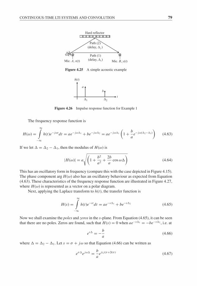
JWBK207-04 JWBK207-Shin January 18, 2008 9:1 Char Count= 0
CONTINUOUS-TIME LTI SYSTEMS AND CONVOLUTION 79
Mic. B, y(t)Mic. A, x(t)
Hard reflector
1
Path (1)(delay, )Δ
2
Path (2)(delay, )Δ
Figure 4.25 A simple acoustic example
1Δ 2Δ
h(t)
ab
t
Figure 4.26 Impulse response function for Example 1
The frequency response function is
H (ω) =∞∫
−∞h(t)e− jωt dt = ae− jω�1 + be− jω�2 = ae− jω�1
(1 + b
ae− jω(�2−�1)
)(4.63)
If we let � = �2 − �1, then the modulus of H (ω) is
|H (ω)| = a
√(1 + b2
a2+ 2b
acos ω�
)(4.64)
This has an oscillatory form in frequency (compare this with the case depicted in Figure 4.15).The phase component arg H (ω) also has an oscillatory behaviour as expected from Equation(4.63). These characteristics of the frequency response function are illustrated in Figure 4.27,where H (ω) is represented as a vector on a polar diagram.
Next, applying the Laplace transform to h(t), the transfer function is
H (s) =∞∫
−∞h(t)e−st dt = ae−s�1 + be−s�2 (4.65)
Now we shall examine the poles and zeros in the s-plane. From Equation (4.65), it can be seenthat there are no poles. Zeros are found, such that H (s) = 0 when ae−s�1 = −be−s�2 , i.e. at
es� = −b
a(4.66)
where � = �2 − �1. Let s = σ + jω so that Equation (4.66) can be written as
eσ�e jω� = b
ae± j(π+2kπ ) (4.67)
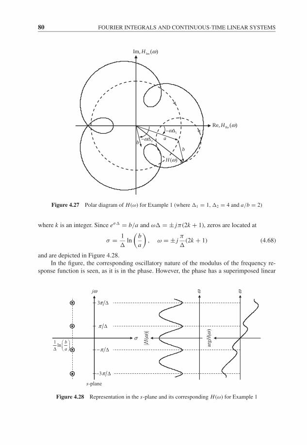
JWBK207-04 JWBK207-Shin January 18, 2008 9:1 Char Count= 0
80 FOURIER INTEGRALS AND CONTINUOUS-TIME LINEAR SYSTEMS
1ω− Δ
2ω− Δ a
b
( )H ω
ReRe, ( )H ω
ImIm, ( )H ω
b
Figure 4.27 Polar diagram of H (ω) for Example 1 (where �1 = 1, �2 = 4 and a/b = 2)
where k is an integer. Since eσ� = b/a and ω� = ± jπ (2k + 1), zeros are located at
σ = 1
�ln
(b
a
), ω = ± j
π
�(2k + 1) (4.68)
and are depicted in Figure 4.28.In the figure, the corresponding oscillatory nature of the modulus of the frequency re-
sponse function is seen, as it is in the phase. However, the phase has a superimposed linear
s-plane
1ln
b
aΔ
3π Δ
jω
σ
ω
|H(ω
)|
arg
H( ω
)
π− Δ
3π− Δ
ω
π Δ
Figure 4.28 Representation in the s-plane and its corresponding H (ω) for Example 1
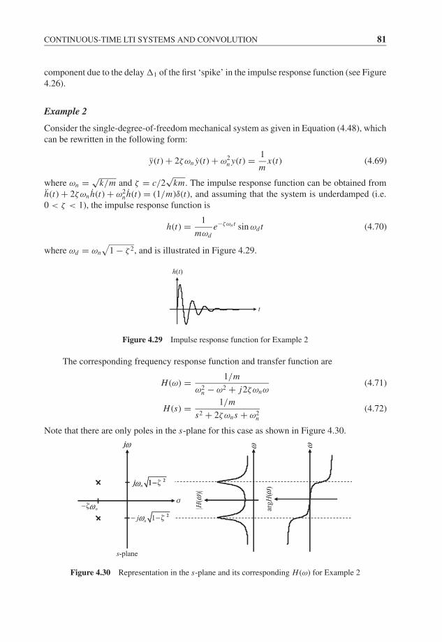
JWBK207-04 JWBK207-Shin January 18, 2008 9:1 Char Count= 0
CONTINUOUS-TIME LTI SYSTEMS AND CONVOLUTION 81
component due to the delay �1 of the first ‘spike’ in the impulse response function (see Figure4.26).
Example 2
Consider the single-degree-of-freedom mechanical system as given in Equation (4.48), whichcan be rewritten in the following form:
y(t) + 2ζωn y(t) + ω2n y(t) = 1
mx(t) (4.69)
where ωn = √k/m and ζ = c/2
√km. The impulse response function can be obtained from
h(t) + 2ζωnh(t) + ω2nh(t) = (1/m)δ(t), and assuming that the system is underdamped (i.e.
0 < ζ < 1), the impulse response function is
h(t) = 1
mωde−ζωn t sin ωd t (4.70)
where ωd = ωn
√1 − ζ 2, and is illustrated in Figure 4.29.
h(t)
t
Figure 4.29 Impulse response function for Example 2
The corresponding frequency response function and transfer function are
H (ω) = 1/m
ω2n − ω2 + j2ζωnω
(4.71)
H (s) = 1/m
s2 + 2ζωns + ω2n
(4.72)
Note that there are only poles in the s-plane for this case as shown in Figure 4.30.
nζω
ω
ω
ω ωω ω
ω−
21nj ζ
ζ
−
2
j
|H(
)|
arg
H(
)
s-plane
21j −
σ
21nj− −
j
Figure 4.30 Representation in the s-plane and its corresponding H (ω) for Example 2
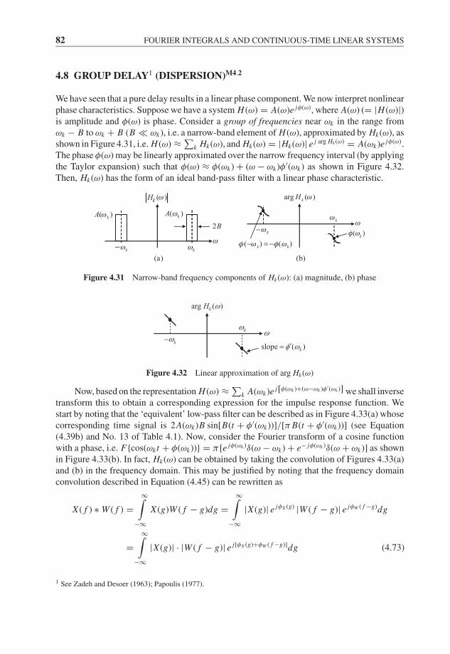
JWBK207-04 JWBK207-Shin January 18, 2008 9:1 Char Count= 0
82 FOURIER INTEGRALS AND CONTINUOUS-TIME LINEAR SYSTEMS
4.8 GROUP DELAY1 (DISPERSION)M4.2
We have seen that a pure delay results in a linear phase component. We now interpret nonlinearphase characteristics. Suppose we have a system H (ω) = A(ω)e jφ(ω), where A(ω) (= |H (ω)|)is amplitude and φ(ω) is phase. Consider a group of frequencies near ωk in the range fromωk − B to ωk + B (B ωk), i.e. a narrow-band element of H (ω), approximated by Hk(ω), asshown in Figure 4.31, i.e. H (ω) ≈ ∑
k Hk(ω), and Hk(ω) = |Hk(ω)| e j arg Hk (ω) = A(ωk)e jφ(ω).The phase φ(ω) may be linearly approximated over the narrow frequency interval (by applyingthe Taylor expansion) such that φ(ω) ≈ φ(ωk) + (ω − ωk)φ′(ωk) as shown in Figure 4.32.Then, Hk(ω) has the form of an ideal band-pass filter with a linear phase characteristic.
( )kA ω
( )kH ω
( )kA ω
arg ( )kH ω
kω
kω− ( )kφ ω− = −
(a) (b)
ω
ω2B
kωk−ω ( ) ( )k kφ ω φ ω
Figure 4.31 Narrow-band frequency components of Hk(ω): (a) magnitude, (b) phase
arg ( )kH ω
kω
kω−slope ( )kφ ω′=
ω
Figure 4.32 Linear approximation of arg Hk(ω)
Now, based on the representation H (ω) ≈ ∑k A(ωk)e j[φ(ωk )+(ω−ωk )φ′(ωk )] we shall inverse
transform this to obtain a corresponding expression for the impulse response function. Westart by noting that the ‘equivalent’ low-pass filter can be described as in Figure 4.33(a) whosecorresponding time signal is 2A(ωk)B sin[B(t + φ′(ωk))]/[π B(t + φ′(ωk))] (see Equation(4.39b) and No. 13 of Table 4.1). Now, consider the Fourier transform of a cosine functionwith a phase, i.e. F{cos(ωk t + φ(ωk))} = π [e jφ(ωk )δ(ω − ωk) + e− jφ(ωk )δ(ω + ωk)] as shownin Figure 4.33(b). In fact, Hk(ω) can be obtained by taking the convolution of Figures 4.33(a)and (b) in the frequency domain. This may be justified by noting that the frequency domainconvolution described in Equation (4.45) can be rewritten as
X ( f ) ∗ W ( f ) =∞∫
−∞X (g)W ( f − g)dg =
∞∫−∞
|X (g)| e jφX (g) |W ( f − g)| e jφW ( f −g)dg
=∞∫
−∞|X (g)| · |W ( f − g)| e j[φX (g)+φW ( f −g)]dg (4.73)
1 See Zadeh and Desoer (1963); Papoulis (1977).

JWBK207-04 JWBK207-Shin January 18, 2008 9:1 Char Count= 0
GROUP DELAY (DISPERSION) 83
1{ }F −
2 ( )kA ωMagnitude:
Phase:
Slope ( )kφ ω′=
(a) Equivalent low-pass filter
kωkω−
( )kφ ω
(b) Fourier transform of carrier
∗(Convolution)
( )( )
( )( )
sin ( )2 ( )
( )
sin ( )2 ( )
( )
k
kk
g k
k
g k
B tA B
B t
B t tA B
B t t
φ ωω
π φ ω
ωω
π ω
′+′+
−=
−
( )
( )
( )cos ( ) cos
cos ( )
kk k k
k
k p k
t t
t t
φ ωω φ ω ωω
ω ω
+ = +
= −×
(Multiplication)
(c) Time domain representation
BB−ω
ω
π π
ω
ωkω
kω−
Figure 4.33 Frequency and time domain representation of Hk(ω)
Thus, the frequency domain convolution (Equation (4.73)) may be interpreted in the form thatthe resultant magnitude is the running sum of the multiplication of two magnitude functionswhile the resultant phase is the running sum of the addition of two phase functions.
Since the convolution in the frequency domain results in the multiplication in the timedomain (see Equation (4.45)) as depicted in Figure 4.33(c), the inverse Fourier transform ofHk(ω) becomes
F−1 {Hk(ω)} ≈ 2A(ωk)Bsin
[B
(t + φ′(ωk)
)]π B (t + φ′(ωk))
cos (ωk t + φ(ωk)) (4.74)
and finally, the inverse Fourier transform of H (ω) is
h(t) = F−1 {H (ω)} ≈∑
k
2A(ωk)Bsin
[B
(t − tg(ωk)
)]π B
(t − tg(ωk)
)︸ ︷︷ ︸envelope
cos ωk(t − tp(ωk))︸ ︷︷ ︸carrier
(4.75)
where tg and tp are the ‘group delay’ and ‘phase delay’ respectively, and are defined byEquations (4.76) and (4.77). The relationship between these two properties is illustrated inFigure 4.34.
tg(ω) = −dφ(ω)
dω(4.76)
tp(ω) = −φ(ω)
ω(4.77)
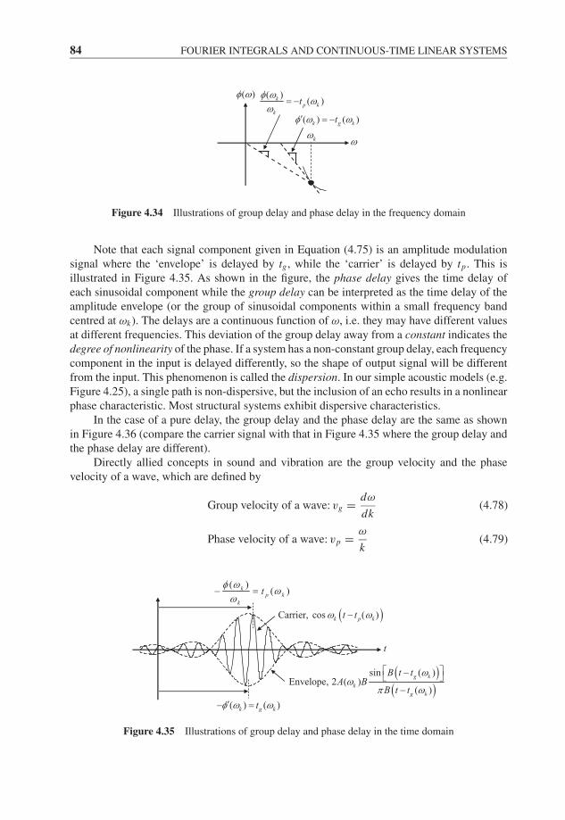
JWBK207-04 JWBK207-Shin January 18, 2008 9:1 Char Count= 0
84 FOURIER INTEGRALS AND CONTINUOUS-TIME LINEAR SYSTEMS
( )φ ω
kω
( )( )k
p kk
tφ ω
ωω
= −
( ) ( )k g ktφ ω ω′ = −
ω
Figure 4.34 Illustrations of group delay and phase delay in the frequency domain
Note that each signal component given in Equation (4.75) is an amplitude modulationsignal where the ‘envelope’ is delayed by tg , while the ‘carrier’ is delayed by tp. This isillustrated in Figure 4.35. As shown in the figure, the phase delay gives the time delay ofeach sinusoidal component while the group delay can be interpreted as the time delay of theamplitude envelope (or the group of sinusoidal components within a small frequency bandcentred at ωk). The delays are a continuous function of ω, i.e. they may have different valuesat different frequencies. This deviation of the group delay away from a constant indicates thedegree of nonlinearity of the phase. If a system has a non-constant group delay, each frequencycomponent in the input is delayed differently, so the shape of output signal will be differentfrom the input. This phenomenon is called the dispersion. In our simple acoustic models (e.g.Figure 4.25), a single path is non-dispersive, but the inclusion of an echo results in a nonlinearphase characteristic. Most structural systems exhibit dispersive characteristics.
In the case of a pure delay, the group delay and the phase delay are the same as shownin Figure 4.36 (compare the carrier signal with that in Figure 4.35 where the group delay andthe phase delay are different).
Directly allied concepts in sound and vibration are the group velocity and the phasevelocity of a wave, which are defined by
Group velocity of a wave: vg = dω
dk(4.78)
Phase velocity of a wave: vp = ω
k(4.79)
t
( ) ( )k g ktφ ω ω′− =
( )( )k
p kk
tφ ω ω
ω− =
( )Carrier, cos ( )k p kt tω ω−
( )( )
sin ( )Envelope, 2 ( )
( )
g k
k
g k
B t tA B
B t t
ωω
π ω
−
−
Figure 4.35 Illustrations of group delay and phase delay in the time domain
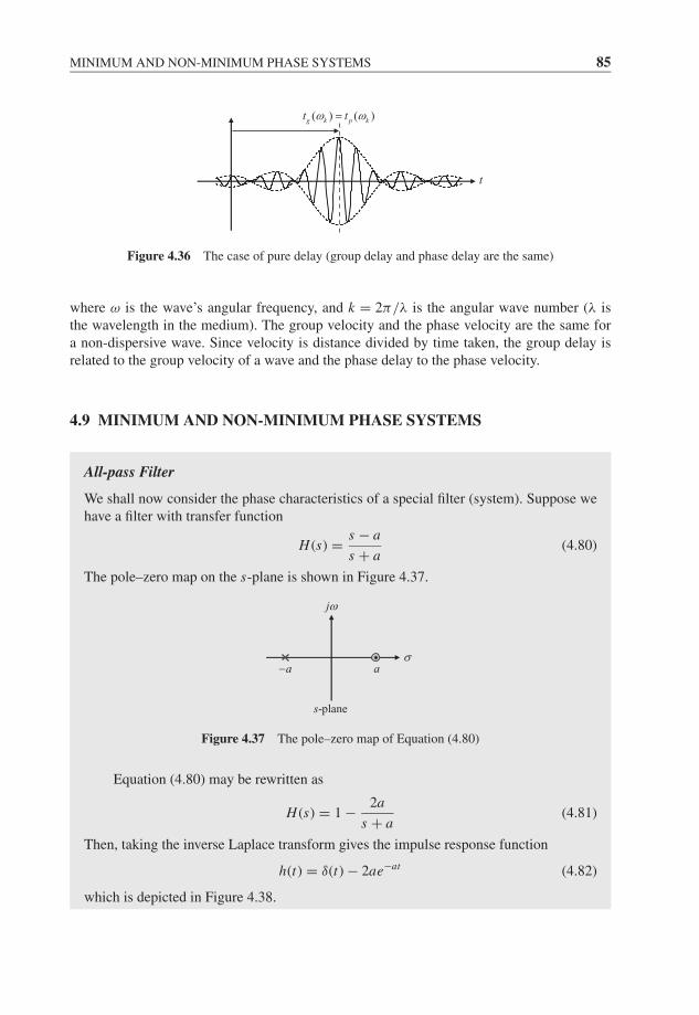
JWBK207-04 JWBK207-Shin January 18, 2008 9:1 Char Count= 0
MINIMUM AND NON-MINIMUM PHASE SYSTEMS 85
( ) ( )g k p kt tω ω=
t
Figure 4.36 The case of pure delay (group delay and phase delay are the same)
where ω is the wave’s angular frequency, and k = 2π/λ is the angular wave number (λ isthe wavelength in the medium). The group velocity and the phase velocity are the same fora non-dispersive wave. Since velocity is distance divided by time taken, the group delay isrelated to the group velocity of a wave and the phase delay to the phase velocity.
4.9 MINIMUM AND NON-MINIMUM PHASE SYSTEMS
All-pass Filter
We shall now consider the phase characteristics of a special filter (system). Suppose wehave a filter with transfer function
H (s) = s − a
s + a(4.80)
The pole–zero map on the s-plane is shown in Figure 4.37.
a−σ
jω
a
s-plane
Figure 4.37 The pole–zero map of Equation (4.80)
Equation (4.80) may be rewritten as
H (s) = 1 − 2a
s + a(4.81)
Then, taking the inverse Laplace transform gives the impulse response function
h(t) = δ(t) − 2ae−at (4.82)
which is depicted in Figure 4.38.
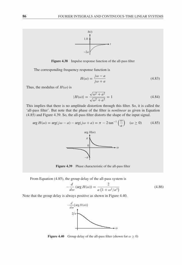
JWBK207-04 JWBK207-Shin January 18, 2008 9:1 Char Count= 0
86 FOURIER INTEGRALS AND CONTINUOUS-TIME LINEAR SYSTEMS
h(t)
1.0
2a−
t
Figure 4.38 Impulse response function of the all-pass filter
The corresponding frequency response function is
H (ω) = jω − a
jω + a(4.83)
Thus, the modulus of H (ω) is
|H (ω)| =√
ω2 + a2
√ω2 + a2
= 1 (4.84)
This implies that there is no amplitude distortion through this filter. So, it is called the‘all-pass filter’. But note that the phase of the filter is nonlinear as given in Equation(4.85) and Figure 4.39. So, the all-pass filter distorts the shape of the input signal.
arg H (ω) = arg( jω − a) − arg( jω + a) = π − 2 tan−1(ω
a
)(ω ≥ 0) (4.85)
arg H(ω)
π−
π
0 ω
Figure 4.39 Phase characteristic of the all-pass filter
From Equation (4.85), the group delay of the all-pass system is
− d
dω(arg H (ω)) = 2
a(1 + ω2/a2
) (4.86)
Note that the group delay is always positive as shown in Figure 4.40.
2 a
ω
( )arg ( )d
Hd
ωω
−
Figure 4.40 Group delay of the all-pass filter (shown for ω ≥ 0)
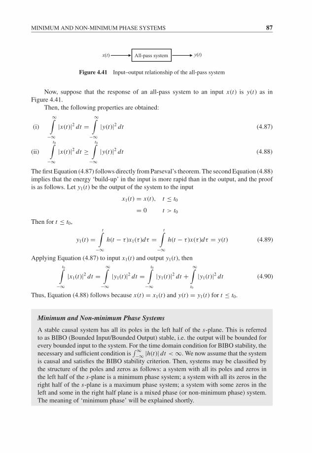
JWBK207-04 JWBK207-Shin January 18, 2008 9:1 Char Count= 0
MINIMUM AND NON-MINIMUM PHASE SYSTEMS 87
All-pass systemx(t) y(t)
Figure 4.41 Input–output relationship of the all-pass system
Now, suppose that the response of an all-pass system to an input x(t) is y(t) as inFigure 4.41.
Then, the following properties are obtained:
(i)
∞∫−∞
|x(t)|2 dt =∞∫
−∞|y(t)|2 dt (4.87)
(ii)
t0∫−∞
|x(t)|2 dt ≥t0∫
−∞|y(t)|2 dt (4.88)
The first Equation (4.87) follows directly from Parseval’s theorem. The second Equation (4.88)implies that the energy ‘build-up’ in the input is more rapid than in the output, and the proofis as follows. Let y1(t) be the output of the system to the input
x1(t) = x(t), t ≤ t0
= 0 t > t0
Then for t ≤ t0,
y1(t) =t∫
−∞h(t − τ )x1(τ )dτ =
t∫−∞
h(t − τ )x(τ )dτ = y(t) (4.89)
Applying Equation (4.87) to input x1(t) and output y1(t), then
t0∫−∞
|x1(t)|2 dt =∞∫
−∞|y1(t)|2 dt =
t0∫−∞
|y1(t)|2 dt +∞∫
t0
|y1(t)|2 dt (4.90)
Thus, Equation (4.88) follows because x(t) = x1(t) and y(t) = y1(t) for t ≤ t0.
Minimum and Non-minimum Phase Systems
A stable causal system has all its poles in the left half of the s-plane. This is referredto as BIBO (Bounded Input/Bounded Output) stable, i.e. the output will be bounded forevery bounded input to the system. For the time domain condition for BIBO stability, thenecessary and sufficient condition is
∫ ∞−∞ |h(t)| dt < ∞. We now assume that the system
is causal and satisfies the BIBO stability criterion. Then, systems may be classified bythe structure of the poles and zeros as follows: a system with all its poles and zeros inthe left half of the s-plane is a minimum phase system; a system with all its zeros in theright half of the s-plane is a maximum phase system; a system with some zeros in theleft and some in the right half plane is a mixed phase (or non-minimum phase) system.The meaning of ‘minimum phase’ will be explained shortly.
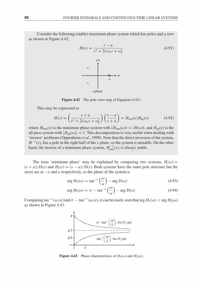
JWBK207-04 JWBK207-Shin January 18, 2008 9:1 Char Count= 0
88 FOURIER INTEGRALS AND CONTINUOUS-TIME LINEAR SYSTEMS
Consider the following (stable) maximum phase system which has poles and a zeroas shown in Figure 4.42:
H (s) = s − a
s2 + 2ζωns + ω2n
(4.91)
σ
jω
a
s-plane
Figure 4.42 The pole–zero map of Equation (4.91)
This may be expressed as
H (s) =(
s + a
s2 + 2ζωns + ω2n
) (s − a
s + a
)= Hmin(s)Hap(s) (4.92)
where Hmin(s) is the minimum phase system with |Hmin(ω)| = |H (ω)|, and Hap(s) is theall-pass system with
∣∣Hap(ω)∣∣ = 1. This decomposition is very useful when dealing with
‘inverse’ problems (Oppenheim et al., 1999). Note that the direct inversion of the system,H−1(s), has a pole in the right half of the s-plane, so the system is unstable. On the otherhand, the inverse of a minimum phase system, H−1
min(s), is always stable.
The term ‘minimum phase’ may be explained by comparing two systems, H1(s) =(s + a)/D(s) and H2(s) = (s − a)/D(s). Both systems have the same pole structure but thezeros are at −a and a respectively, so the phase of the system is
arg H1(ω) = tan−1(ω
a
)− arg D(ω) (4.93)
arg H2(ω) = π − tan−1(ω
a
)− arg D(ω) (4.94)
Comparing tan−1 (ω/a) and π − tan−1 (ω/a), it can be easily seen that arg H1(ω) < arg H2(ω)as shown in Figure 4.43.
2π
4π
π
ω
1
2tan , for ( )Haωπ ω−−
1
1tan , for ( )Haω ω−
a
Figure 4.43 Phase characteristics of H1(ω) and H2(ω)
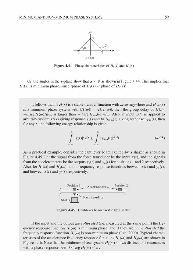
JWBK207-04 JWBK207-Shin January 18, 2008 9:1 Char Count= 0
MINIMUM AND NON-MINIMUM PHASE SYSTEMS 89
a−σ
jω
a
α β
ω
s-plane
Figure 4.44 Phase characteristics of H1(s) and H2(s)
Or, the angles in the s-plane show that α < β as shown in Figure 4.44. This implies thatH1(s) is minimum phase, since ‘phase of H1(s) < phase of H2(s)’.
It follows that, if H (s) is a stable transfer function with zeros anywhere and Hmin(s)is a minimum phase system with |H (ω)| = |Hmin(ω)|, then the group delay of H (s),−d arg H (ω)/dω, is larger than −d arg Hmin(ω)/dω. Also, if input x(t) is applied toarbitrary system H (s) giving response y(t) and to Hmin(s) giving response ymin(t), thenfor any t0 the following energy relationship is given:
t0∫−∞
|y(t)|2 dt ≥t0∫
−∞|ymin(t)|2 dt (4.95)
As a practical example, consider the cantilever beam excited by a shaker as shown inFigure 4.45. Let the signal from the force transducer be the input x(t), and the signalsfrom the accelerometers be the outputs y1(t) and y2(t) for positions 1 and 2 respectively.Also, let H1(ω) and H2(ω) be the frequency response functions between x(t) and y1(t),and between x(t) and y2(t) respectively.
Position 1 Position 2Accelerometer
Force transducerShaker
Figure 4.45 Cantilever beam excited by a shaker
If the input and the output are collocated (i.e. measured at the same point) the fre-quency response function H1(ω) is minimum phase, and if they are non-collocated thefrequency response function H2(ω) is non-minimum phase (Lee, 2000). Typical charac-teristics of the accelerance frequency response functions H1(ω) and H2(ω) are shown inFigure 4.46. Note that the minimum phase system H1(ω) shows distinct anti-resonanceswith a phase response over 0 ≤ arg H1(ω) ≤ π .
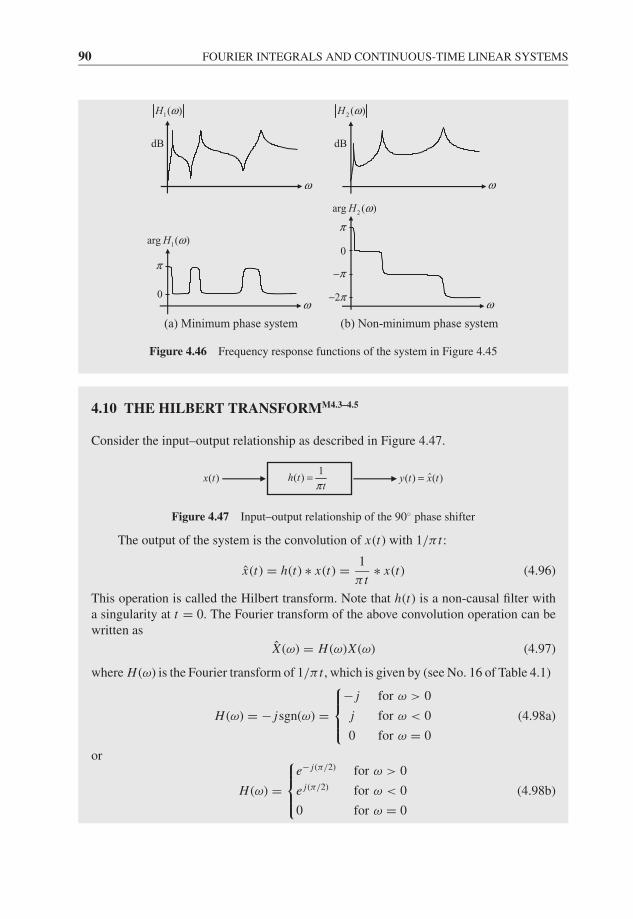
JWBK207-04 JWBK207-Shin January 18, 2008 9:1 Char Count= 0
90 FOURIER INTEGRALS AND CONTINUOUS-TIME LINEAR SYSTEMS
2arg ( )H ω
π
2π−
0
π−
ω
2 ( )H ω
ω
dB
(b) Non-minimum phase system
1arg ( )H ω
ω
π
0
(a) Minimum phase system
ω
dB
1( )H ω
Figure 4.46 Frequency response functions of the system in Figure 4.45
4.10 THE HILBERT TRANSFORMM4.3–4.5
Consider the input–output relationship as described in Figure 4.47.
1( )h t
tπ= ˆ( ) ( )y t x t=( )x t
Figure 4.47 Input–output relationship of the 90◦ phase shifter
The output of the system is the convolution of x(t) with 1/π t :
x(t) = h(t) ∗ x(t) = 1
π t∗ x(t) (4.96)
This operation is called the Hilbert transform. Note that h(t) is a non-causal filter witha singularity at t = 0. The Fourier transform of the above convolution operation can bewritten as
X (ω) = H (ω)X (ω) (4.97)
where H (ω) is the Fourier transform of 1/π t , which is given by (see No. 16 of Table 4.1)
H (ω) = − jsgn(ω) =
⎧⎪⎨⎪⎩− j for ω > 0
j for ω < 0
0 for ω = 0
(4.98a)
or
H (ω) =
⎧⎪⎨⎪⎩e− j(π/2) for ω > 0
e j(π/2) for ω < 0
0 for ω = 0
(4.98b)
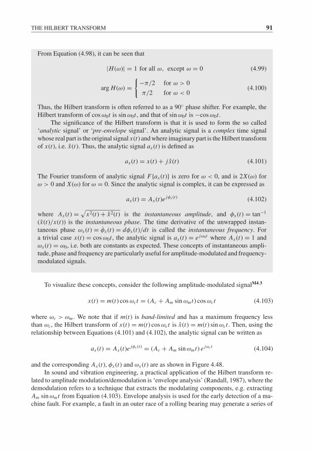
JWBK207-04 JWBK207-Shin January 18, 2008 9:1 Char Count= 0
THE HILBERT TRANSFORM 91
From Equation (4.98), it can be seen that
|H (ω)| = 1 for all ω, except ω = 0 (4.99)
arg H (ω) ={
−π/2 for ω > 0
π/2 for ω < 0(4.100)
Thus, the Hilbert transform is often referred to as a 90◦ phase shifter. For example, theHilbert transform of cos ω0t is sin ω0t , and that of sin ω0t is −cos ω0t .
The significance of the Hilbert transform is that it is used to form the so called‘analytic signal’ or ‘pre-envelope signal’. An analytic signal is a complex time signalwhose real part is the original signal x(t) and where imaginary part is the Hilbert transformof x(t), i.e. x(t). Thus, the analytic signal ax (t) is defined as
ax (t) = x(t) + j x(t) (4.101)
The Fourier transform of analytic signal F{ax (t)} is zero for ω < 0, and is 2X (ω) forω > 0 and X (ω) for ω = 0. Since the analytic signal is complex, it can be expressed as
ax (t) = Ax (t)e jφx (t) (4.102)
where Ax (t) =√
x2(t) + x2(t) is the instantaneous amplitude, and φx (t) = tan−1
(x(t)/x(t)) is the instantaneous phase. The time derivative of the unwrapped instan-taneous phase ωx (t) = φx (t) = dφx (t)/dt is called the instantaneous frequency. Fora trivial case x(t) = cos ω0t , the analytic signal is ax (t) = e jω0t where Ax (t) = 1 andωx (t) = ω0, i.e. both are constants as expected. These concepts of instantaneous ampli-tude, phase and frequency are particularly useful for amplitude-modulated and frequency-modulated signals.
To visualize these concepts, consider the following amplitude-modulated signalM4.3
x(t) = m(t) cos ωct = (Ac + Am sin ωmt) cos ωct (4.103)
where ωc > ωm . We note that if m(t) is band-limited and has a maximum frequency lessthan ωc, the Hilbert transform of x(t) = m(t) cos ωct is x(t) = m(t) sin ωct . Then, using therelationship between Equations (4.101) and (4.102), the analytic signal can be written as
ax (t) = Ax (t)e jφx (t) = (Ac + Am sin ωmt) e jωct (4.104)
and the corresponding Ax (t), φx (t) and ωx (t) are as shown in Figure 4.48.In sound and vibration engineering, a practical application of the Hilbert transform re-
lated to amplitude modulation/demodulation is ‘envelope analysis’ (Randall, 1987), where thedemodulation refers to a technique that extracts the modulating components, e.g. extractingAm sin ωmt from Equation (4.103). Envelope analysis is used for the early detection of a ma-chine fault. For example, a fault in an outer race of a rolling bearing may generate a series of

JWBK207-04 JWBK207-Shin January 18, 2008 9:1 Char Count= 0
92 FOURIER INTEGRALS AND CONTINUOUS-TIME LINEAR SYSTEMS
t
( )x tφ
t
( )x tω
cω
(c) Instantaneous frequency
( )c mA A− +
t
c mA A+ ( )xA t
( )x t
(a) Instantaneous amplitude
(b) Instantaneous (unwrapped) phase
Figure 4.48 Analytic signal associated with the amplitude-modulated signal
burst signals at a regular interval. Such burst signals decay very quickly and contain relativelysmall energies, thus the usual Fourier analysis may not reveal the repetition frequency of thebursts. However, it may be possible to detect this frequency component by forming the analyticsignal and then applying Fourier analysis to the envelope Ax (t).
Examples
Example 1: Estimation of damping from time domain recordsof an oscillator M4.4
Suppose we have a free response of a damped single-degree-of-freedom system as below:
x(t) = Ae−ζωn t sin(ωd t + φ) t ≥ 0 (4.105)
where ωd = ωn
√1 − ζ 2. The analytic signal for this may be approximated as
ax (t) = Ax (t)e jφx (t) ≈ (Ae−ζωn t
)e j(ωd t+φ−π/2) t ≥ 0 (4.106)
Since ln Ax (t) ≈ ln A − ζωnt , the damping ratio ζ can be estimated from the plot of ln Ax (t)versus time, provided that the natural frequencyωn is known. This is demonstrated in MATLABExample 4.4. However, as shown in MATLAB Example 4.4, it must be noted that Ax (t) andφx (t) are usually distorted, especially at the beginning and the last parts of the signal. Thisundesirable phenomenon occurs from the following: (i) the modulating component Ae−ζωn t
is not band-limited, (ii) the non-causal nature of the filter (h(t) = 1/π t), and (iii) practicalwindowing effects (truncation in the frequency domain). Thus, the part of the signal neart = 0 must be avoided in the estimation of the damping characteristic. The windowing effectis discussed in the next section.
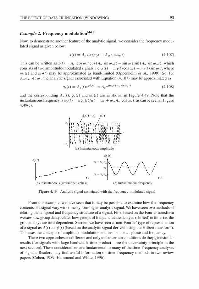
JWBK207-04 JWBK207-Shin January 18, 2008 9:1 Char Count= 0
THE EFFECT OF DATA TRUNCATION (WINDOWING) 93
Example 2: Frequency modulationM4.5
Now, to demonstrate another feature of the analytic signal, we consider the frequency modu-lated signal as given below:
x(t) = Ac cos(ωct + Am sin ωmt) (4.107)
This can be written as x(t) = Ac [cos ωct cos (Am sin ωmt) − sin ωct sin (Am sin ωmt)] whichconsists of two amplitude-modulated signals, i.e. x(t) = m1(t) cos ωct − m2(t) sin ωct , wherem1(t) and m2(t) may be approximated as band-limited (Oppenheim et al., 1999). So, forAmωm ωc, the analytic signal associated with Equation (4.107) may be approximated as
ax (t) = Ax (t)e jφx (t) ≈ Ace j(ωct+Am sin ωm t) (4.108)
and the corresponding Ax (t), φx (t) and ωx (t) are as shown in Figure 4.49. Note that theinstantaneous frequency is ωx (t) = dφx (t)/dt = ωc + ωm Am cos ωmt , as can be seen in Figure4.49(c).
( )x tφ
t
(c) Instantaneous frequency
(a) Instantaneous amplitude
(b) Instantaneous (unwrapped) phase
cA−
t
cA
( )x cA t A≈ ( )x t
( )x tω
cω
t
c m mAω ω+
c m mAω ω−
Figure 4.49 Analytic signal associated with the frequency-modulated signal
From this example, we have seen that it may be possible to examine how the frequencycontents of a signal vary with time by forming an analytic signal. We have seen two methods ofrelating the temporal and frequency structure of a signal. First, based on the Fourier transformwe saw how group delay relates how groups of frequencies are delayed (shifted) in time, i.e. thegroup delays are time dependent. Second, we have seen a ‘non-Fourier’ type of representationof a signal as A(t) cos φ(t) (based on the analytic signal derived using the Hilbert transform).This uses the concepts of amplitude modulation and instantaneous phase and frequency.
These two approaches are different and only under certain conditions do they give similarresults (for signals with large bandwidth–time product – see the uncertainty principle in thenext section). These considerations are fundamental to many of the time–frequency analysesof signals. Readers may find useful information on time–frequency methods in two reviewpapers (Cohen, 1989; Hammond and White, 1996).
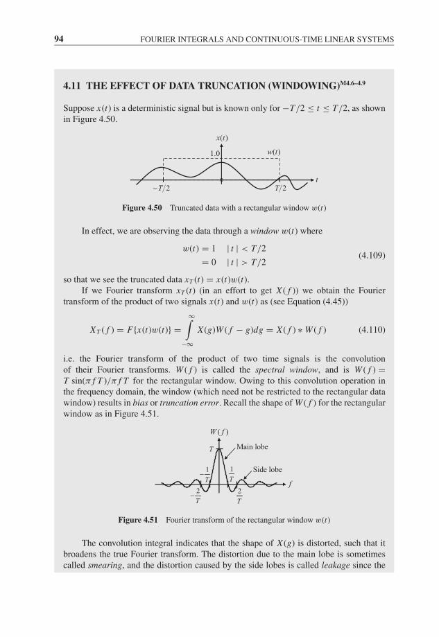
JWBK207-04 JWBK207-Shin January 18, 2008 9:1 Char Count= 0
94 FOURIER INTEGRALS AND CONTINUOUS-TIME LINEAR SYSTEMS
4.11 THE EFFECT OF DATA TRUNCATION (WINDOWING)M4.6–4.9
Suppose x(t) is a deterministic signal but is known only for −T/2 ≤ t ≤ T/2, as shownin Figure 4.50.
2T2T−t
( )w t
( )x t
1.0
Figure 4.50 Truncated data with a rectangular window w(t)
In effect, we are observing the data through a window w(t) where
w(t) = 1 | t | < T/2
= 0 | t | > T/2(4.109)
so that we see the truncated data xT (t) = x(t)w(t).If we Fourier transform xT (t) (in an effort to get X ( f )) we obtain the Fourier
transform of the product of two signals x(t) and w(t) as (see Equation (4.45))
XT ( f ) = F{x(t)w(t)} =∞∫
−∞X (g)W ( f − g)dg = X ( f ) ∗ W ( f ) (4.110)
i.e. the Fourier transform of the product of two time signals is the convolutionof their Fourier transforms. W ( f ) is called the spectral window, and is W ( f ) =T sin(π f T )/π f T for the rectangular window. Owing to this convolution operation inthe frequency domain, the window (which need not be restricted to the rectangular datawindow) results in bias or truncation error. Recall the shape of W ( f ) for the rectangularwindow as in Figure 4.51.
1
T
2
T
1
T−
2
T−
Side lobe
Main lobeT
( )W f
f
Figure 4.51 Fourier transform of the rectangular window w(t)
The convolution integral indicates that the shape of X (g) is distorted, such that itbroadens the true Fourier transform. The distortion due to the main lobe is sometimescalled smearing, and the distortion caused by the side lobes is called leakage since the

JWBK207-04 JWBK207-Shin January 18, 2008 9:1 Char Count= 0
THE EFFECT OF DATA TRUNCATION (WINDOWING) 95
frequency components of X (g) at values other than g = f ‘leak’ through the side lobesto contribute to the value of XT ( f ) at f . For example, consider a sinusoidal signalx(t) = cos(2πpt) whose Fourier transform is X ( f ) = 1
2[δ( f + p) + δ( f − p)]. Then
the Fourier transform of the truncated signal xT (t) is
XT ( f ) =∞∫
−∞X (g)W ( f − g)dg = 1
2
∞∫−∞
[δ(g + p) + δ(g − p)] W ( f − g)dg
= 1
2[W ( f + p) + W ( f − p)] (4.111)
This shows that the delta functions (in the frequency domain) are replaced by the shape ofthe spectral window. The ‘theoretical’ and ‘achieved (windowed)’ spectra are illustratedin Figure 4.52 (compare X ( f ) and XT ( f ) for both shape and magnitude).
1 21 2
( )X f
(a) Theoretical
fpp−
( ) ( ) ( )TX f X f W f= ∗
fpp−
2T Smearing
Leakage
(b) Windowed
Figure 4.52 Fourier transform of a cosine wave
If two or more closely spaced sinusoidal components are present in a signal, then theymay not easily be resolved in the frequency domain because of the distortion (especiallydue to the main lobe). A rough guide as to the effect of this rectangular window is obtainedfrom Figure 4.53 (shown for f > 0 only).
0f
Considerable smearing due to
the spectral window
Three components are resolved but with
considerable leakage at other frequencies
Tin
crea
ses
1f 2ff
( )X f
f
f
0f 1f 2f
0f 1f 2f
( )TX f
( )TX f
x(t) is the sum of three sine (or cosine) waves
Figure 4.53 Effects of windowing on the modulus of the Fourier transform
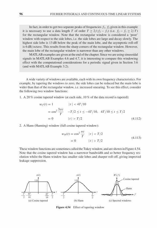
JWBK207-04 JWBK207-Shin January 18, 2008 9:1 Char Count= 0
96 FOURIER INTEGRALS AND CONTINUOUS-TIME LINEAR SYSTEMS
In fact, in order to get two separate peaks of frequencies f1, f2 given in this exampleit is necessary to use a data length T of order T ≥ 2/( f2 − f1) (i.e. f2 − f1 ≥ 2/T )for the rectangular window. Note that the rectangular window is considered a ‘poor’window with respect to the side lobes, i.e. the side lobes are large and decay slowly. Thehighest side lobe is 13 dB below the peak of the main lobe, and the asymptotic roll-offis 6 dB/octave. This results from the sharp corners of the rectangular window. However,the main lobe of the rectangular window is narrower than any other windows.
MATLAB examples are given at the end of the chapter. Since we are using sinusoidalsignals in MATLAB Examples 4.6 and 4.7, it is interesting to compare this windowingeffect with the computational considerations for a periodic signal given in Section 3.6(and with MATLAB Example 3.2).
A wide variety of windows are available, each with its own frequency characteristics. Forexample, by tapering the windows to zero, the side lobes can be reduced but the main lobe iswider than that of the rectangular window, i.e. increased smearing. To see this effect, considerthe following two window functions:
1. A 20 % cosine tapered window (at each side, 10 % of the data record is tapered):
wC (t) = 1 | t | < 4T /10
= cos2 5π t
T−T /2 ≤ t ≤ −4T /10, 4T /10 ≤ t ≤ T/2
= 0 | t | > T/2 (4.112)
2. A Hann (Hanning) window (full cosine tapered window):
wH (t) = cos2 π t
T| t | < T/2
(4.113)= 0 | t | > T/2
These window functions are sometimes called the Tukey window, and are shown in Figure 4.54.Note that the cosine tapered window has a narrower bandwidth and so better frequency res-olution whilst the Hann window has smaller side lobes and sharper roll-off, giving improvedleakage suppression.
(a) Cosine tapered (b) Hann
( )x t
1.0
2
T−2
T4
10
T− 4
10
Ttt
2
T
2
T−
1.0
( )x t
f
( )W f
Cosine tapered
Hann
(c) Spectral windows
Figure 4.54 Effect of tapering window
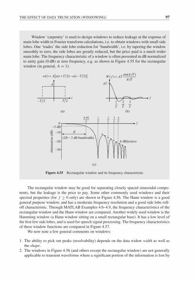
JWBK207-04 JWBK207-Shin January 18, 2008 9:1 Char Count= 0
THE EFFECT OF DATA TRUNCATION (WINDOWING) 97
Window ‘carpentry’ is used to design windows to reduce leakage at the expense ofmain lobe width in Fourier transform calculations, i.e. to obtain windows with small sidelobes. One ‘trades’ the side lobe reduction for ‘bandwidth’, i.e. by tapering the windowsmoothly to zero, the side lobes are greatly reduced, but the price paid is a much widermain lobe. The frequency characteristic of a window is often presented in dB normalizedto unity gain (0 dB) at zero frequency, e.g. as shown in Figure 4.55 for the rectangularwindow (in general, A = 1).
(a)
[ ]( ) ( 2) ( 2)w t A u t T u t T= + − −
2T2T−
A
t
(b)
sin( )( )
fTW f AT
fT
ππ
=
2
T
1
T
3
T
AT
f
Att
enu
atio
n (
dB
)
(2B = 3 dB bandwidth)
−30
−20
−10
0−3 dB
B
0.44
T
1
T
2
T
3
T
4
T
6 dB octave
f
(c)
Figure 4.55 Rectangular window and its frequency characteristic
The rectangular window may be good for separating closely spaced sinusoidal compo-nents, but the leakage is the price to pay. Some other commonly used windows and theirspectral properties (for f ≥ 0 only) are shown in Figure 4.56. The Hann window is a goodgeneral purpose window, and has a moderate frequency resolution and a good side lobe roll-off characteristic. Through MATLAB Examples 4.6–4.9, the frequency characteristics of therectangular window and the Hann window are compared. Another widely used window is theHamming window (a Hann window sitting on a small rectangular base). It has a low level ofthe first few side lobes, and is used for speech signal processing. The frequency characteristicsof these window functions are compared in Figure 4.57.
We now note a few general comments on windows:
1. The ability to pick out peaks (resolvability) depends on the data widow width as well asthe shape.
2. The windows in Figure 4.56 (and others except the rectangular window) are not generallyapplicable to transient waveforms where a significant portion of the information is lost by

JWBK207-04 JWBK207-Shin January 18, 2008 9:1 Char Count= 0
98 FOURIER INTEGRALS AND CONTINUOUS-TIME LINEAR SYSTEMS
(a) Bartlett window (in general, A = 1)
otherwise0
tw(t) tA 1 T 2
T 2−= ≤
=
T 2T 2−
w(t)
A
t
2
sin(
2
AT f T 2)W(f )
f T 2
ππ
=
2
T
4
T
AT 2
W(f )
f
(b) Hann window (in general, A = 1)
2 2cos1
2
otherwise0
At tw(t) tAcos T 2
TT
ππ == ≤+
=
w(t)
A
T 2T 2−t
2
sin(
2 (f T )
AT f T )W(f )
f T 1
ππ
⋅=−
W(f )
f2
T
3
T
AT 2
(c) Hamming window
W(f )
f2
T
3
T
0.54
22
22
0.54 0.08( sin(
(
f T ) f T )W(f )
fT f T )
ππ πππ π
−=
−
w(t)
T 2T 2−t
20.54 0.46 cos
otherwise0
tw(t) T 2t
T
π+= ≤
=
1.0
(d) Parzen window
4
T
4
sin(3T
8
f T 4)W(f )
f T 4
ππ
=
3T 8
f
W(f )
32
3
241 484
2 14 2
0 otherwise
tt Tw(t) t
TT
t TTt
T 2
−= ≤+
−= ≤<
=
T 2T 2−
w(t)
1.0
t
Figure 4.56 Some commonly used windows
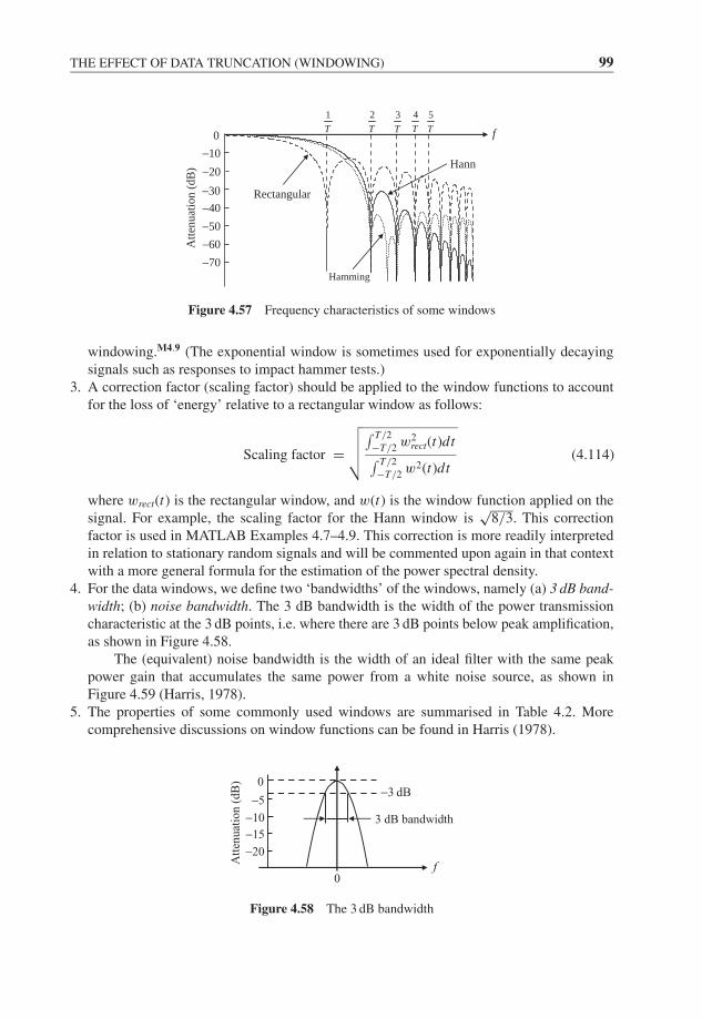
JWBK207-04 JWBK207-Shin January 18, 2008 9:1 Char Count= 0
THE EFFECT OF DATA TRUNCATION (WINDOWING) 99
Atte
nuat
ion
(dB
)
f
−40
−30
−20
−10
0
1T
2T
3T
4T
Rectangular
Hann
−50
−60
−70
5T
Hamming
Figure 4.57 Frequency characteristics of some windows
windowing.M4.9 (The exponential window is sometimes used for exponentially decayingsignals such as responses to impact hammer tests.)
3. A correction factor (scaling factor) should be applied to the window functions to accountfor the loss of ‘energy’ relative to a rectangular window as follows:
Scaling factor =√√√√∫ T/2
−T/2w2
rect(t)dt∫ T/2
−T/2w2(t)dt
(4.114)
where wrect(t) is the rectangular window, and w(t) is the window function applied on thesignal. For example, the scaling factor for the Hann window is
√8/3. This correction
factor is used in MATLAB Examples 4.7–4.9. This correction is more readily interpretedin relation to stationary random signals and will be commented upon again in that contextwith a more general formula for the estimation of the power spectral density.
4. For the data windows, we define two ‘bandwidths’ of the windows, namely (a) 3 dB band-width; (b) noise bandwidth. The 3 dB bandwidth is the width of the power transmissioncharacteristic at the 3 dB points, i.e. where there are 3 dB points below peak amplification,as shown in Figure 4.58.
The (equivalent) noise bandwidth is the width of an ideal filter with the same peakpower gain that accumulates the same power from a white noise source, as shown inFigure 4.59 (Harris, 1978).
5. The properties of some commonly used windows are summarised in Table 4.2. Morecomprehensive discussions on window functions can be found in Harris (1978).
Att
enu
atio
n (
dB
)
3 dB bandwidth
−20
−15
−10
−5
0
f
3 dB−
0
Figure 4.58 The 3 dB bandwidth
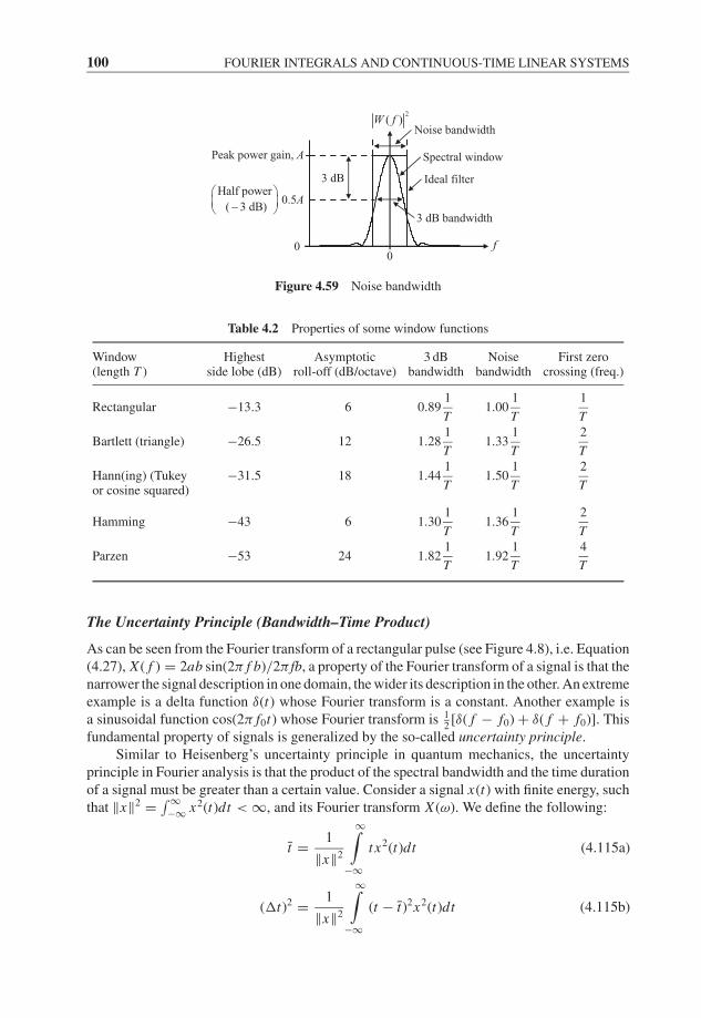
JWBK207-04 JWBK207-Shin January 18, 2008 9:1 Char Count= 0
100 FOURIER INTEGRALS AND CONTINUOUS-TIME LINEAR SYSTEMS
2( )W f
Peak power gain, A
0
0.5A
Spectral window
Ideal filter
3 dB bandwidth
Noise bandwidth
3 dB
f
Half power
( 3 dB)−
0
Figure 4.59 Noise bandwidth
Table 4.2 Properties of some window functions
Window Highest Asymptotic 3 dB Noise First zero(length T ) side lobe (dB) roll-off (dB/octave) bandwidth bandwidth crossing (freq.)
Rectangular −13.3 6 0.891
T1.00
1
T
1
T
Bartlett (triangle) −26.5 12 1.281
T1.33
1
T
2
T
Hann(ing) (Tukeyor cosine squared)
−31.5 18 1.441
T1.50
1
T
2
T
Hamming −43 6 1.301
T1.36
1
T
2
T
Parzen −53 24 1.821
T1.92
1
T
4
T
The Uncertainty Principle (Bandwidth–Time Product)
As can be seen from the Fourier transform of a rectangular pulse (see Figure 4.8), i.e. Equation(4.27), X ( f ) = 2ab sin(2π f b)/2π fb, a property of the Fourier transform of a signal is that thenarrower the signal description in one domain, the wider its description in the other. An extremeexample is a delta function δ(t) whose Fourier transform is a constant. Another example isa sinusoidal function cos(2π f0t) whose Fourier transform is 1
2[δ( f − f0) + δ( f + f0)]. This
fundamental property of signals is generalized by the so-called uncertainty principle.Similar to Heisenberg’s uncertainty principle in quantum mechanics, the uncertainty
principle in Fourier analysis is that the product of the spectral bandwidth and the time durationof a signal must be greater than a certain value. Consider a signal x(t) with finite energy, suchthat ‖x‖2 = ∫ ∞
−∞ x2(t)dt < ∞, and its Fourier transform X (ω). We define the following:
t = 1
‖x‖2
∞∫−∞
t x2(t)dt (4.115a)
(�t)2 = 1
‖x‖2
∞∫−∞
(t − t)2x2(t)dt (4.115b)
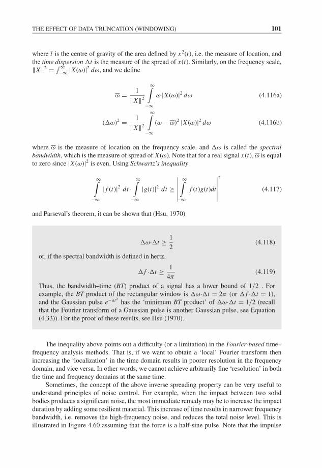
JWBK207-04 JWBK207-Shin January 18, 2008 9:1 Char Count= 0
THE EFFECT OF DATA TRUNCATION (WINDOWING) 101
where t is the centre of gravity of the area defined by x2(t), i.e. the measure of location, andthe time dispersion �t is the measure of the spread of x(t). Similarly, on the frequency scale,‖X‖2 = ∫ ∞
−∞ |X (ω)|2 dω, and we define
ω = 1
‖X‖2
∞∫−∞
ω |X (ω)|2 dω (4.116a)
(�ω)2 = 1
‖X‖2
∞∫−∞
(ω − ω)2 |X (ω)|2 dω (4.116b)
where ω is the measure of location on the frequency scale, and �ω is called the spectralbandwidth, which is the measure of spread of X (ω). Note that for a real signal x(t), ω is equalto zero since |X (ω)|2 is even. Using Schwartz’s inequality
∞∫−∞
| f (t)|2 dt ·∞∫
−∞|g(t)|2 dt ≥
∣∣∣∣∣∣∞∫
−∞f (t)g(t)dt
∣∣∣∣∣∣2
(4.117)
and Parseval’s theorem, it can be shown that (Hsu, 1970)
�ω·�t ≥ 1
2(4.118)
or, if the spectral bandwidth is defined in hertz,
� f ·�t ≥ 1
4π(4.119)
Thus, the bandwidth–time (BT) product of a signal has a lower bound of 1/2 . Forexample, the BT product of the rectangular window is �ω·�t = 2π (or � f ·�t = 1),and the Gaussian pulse e−at2
has the ‘minimum BT product’ of �ω·�t = 1/2 (recallthat the Fourier transform of a Gaussian pulse is another Gaussian pulse, see Equation(4.33)). For the proof of these results, see Hsu (1970).
The inequality above points out a difficulty (or a limitation) in the Fourier-based time–frequency analysis methods. That is, if we want to obtain a ‘local’ Fourier transform thenincreasing the ‘localization’ in the time domain results in poorer resolution in the frequencydomain, and vice versa. In other words, we cannot achieve arbitrarily fine ‘resolution’ in boththe time and frequency domains at the same time.
Sometimes, the concept of the above inverse spreading property can be very useful tounderstand principles of noise control. For example, when the impact between two solidbodies produces a significant noise, the most immediate remedy may be to increase the impactduration by adding some resilient material. This increase of time results in narrower frequencybandwidth, i.e. removes the high-frequency noise, and reduces the total noise level. This isillustrated in Figure 4.60 assuming that the force is a half-sine pulse. Note that the impulse
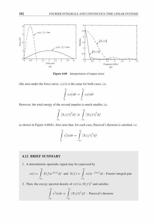
JWBK207-04 JWBK207-Shin January 18, 2008 9:1 Char Count= 0
102 FOURIER INTEGRALS AND CONTINUOUS-TIME LINEAR SYSTEMS
0 0.5 1 1.5 2 2.5 3 3.5 40
1
2
3
4
Time (ms)
Forc
e (N
)
1 1( ), 1msx t T =
2 2( ), 4 msx t T =
(a)
0 0.5 1 1.5 2 2.5 3 3.50
0.5
1
1.5
2
2.5
3
Frequency (kHz)
Mo
dulu
s
2 ( )X f
(b)
1( )X f
Figure 4.60 Interpretation of impact noise
(the area under the force curve, xi (t)) is the same for both cases, i.e.
T1∫0
x1(t)dt =T2∫
0
x2(t)dt
However, the total energy of the second impulse is much smaller, i.e.
∞∫−∞
∣∣X1( f )∣∣2
d f �∞∫
−∞
∣∣X2( f )∣∣2
d f
as shown in Figure 4.60(b). Also note that, for each case, Parseval’s theorem is satisfied, i.e.
Ti∫0
x2i (t)dt =
∞∫−∞
∣∣Xi ( f )∣∣2
d f
4.12 BRIEF SUMMARY
1. A deterministic aperiodic signal may be expressed by
x(t) =∞∫
−∞X ( f )e j2π f t d f and X ( f ) =
∞∫−∞
x(t)e− j2π f t dt : Fourier integral pair
2. Then, the energy spectral density of x(t) is |X ( f )|2 and satisfies
∞∫−∞
x2(t)dt =∞∫
−∞|X ( f )|2 d f : Parseval’s theorem
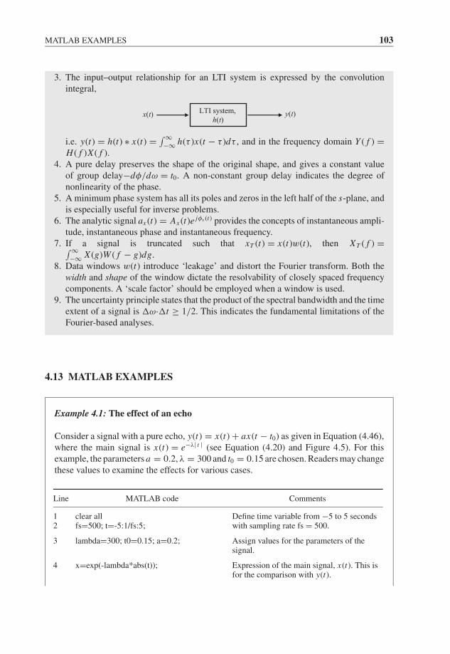
JWBK207-04 JWBK207-Shin January 18, 2008 9:1 Char Count= 0
MATLAB EXAMPLES 103
3. The input–output relationship for an LTI system is expressed by the convolutionintegral,
LTI system, h(t)
x(t) y(t)
i.e. y(t) = h(t) ∗ x(t) = ∫ ∞−∞ h(τ )x(t − τ )dτ , and in the frequency domain Y ( f ) =
H ( f )X ( f ).4. A pure delay preserves the shape of the original shape, and gives a constant value
of group delay−dφ/dω = t0. A non-constant group delay indicates the degree ofnonlinearity of the phase.
5. A minimum phase system has all its poles and zeros in the left half of the s-plane, andis especially useful for inverse problems.
6. The analytic signal ax (t) = Ax (t)e jφx (t) provides the concepts of instantaneous ampli-tude, instantaneous phase and instantaneous frequency.
7. If a signal is truncated such that xT (t) = x(t)w(t), then XT ( f ) =∫ ∞−∞ X (g)W ( f − g)dg.
8. Data windows w(t) introduce ‘leakage’ and distort the Fourier transform. Both thewidth and shape of the window dictate the resolvability of closely spaced frequencycomponents. A ‘scale factor’ should be employed when a window is used.
9. The uncertainty principle states that the product of the spectral bandwidth and the timeextent of a signal is �ω·�t ≥ 1/2. This indicates the fundamental limitations of theFourier-based analyses.
4.13 MATLAB EXAMPLES
Example 4.1: The effect of an echo
Consider a signal with a pure echo, y(t) = x(t) + ax(t − t0) as given in Equation (4.46),where the main signal is x(t) = e−λ| t | (see Equation (4.20) and Figure 4.5). For thisexample, the parameters a = 0.2, λ = 300 and t0 = 0.15 are chosen. Readers may changethese values to examine the effects for various cases.
Line MATLAB code Comments
12
clear allfs=500; t=-5:1/fs:5;
Define time variable from −5 to 5 secondswith sampling rate fs = 500.
3 lambda=300; t0=0.15; a=0.2; Assign values for the parameters of thesignal.
4 x=exp(-lambda*abs(t)); Expression of the main signal, x(t). This isfor the comparison with y(t).
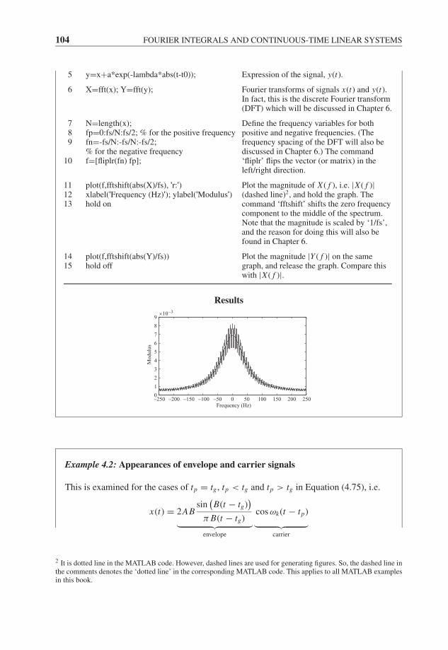
JWBK207-04 JWBK207-Shin January 18, 2008 9:1 Char Count= 0
104 FOURIER INTEGRALS AND CONTINUOUS-TIME LINEAR SYSTEMS
5 y=x+a*exp(-lambda*abs(t-t0)); Expression of the signal, y(t).
6 X=fft(x); Y=fft(y); Fourier transforms of signals x(t) and y(t).In fact, this is the discrete Fourier transform(DFT) which will be discussed in Chapter 6.
789
10
N=length(x);fp=0:fs/N:fs/2; % for the positive frequencyfn=-fs/N:-fs/N:-fs/2;% for the negative frequencyf=[fliplr(fn) fp];
Define the frequency variables for bothpositive and negative frequencies. (Thefrequency spacing of the DFT will also bediscussed in Chapter 6.) The command‘fliplr’ flips the vector (or matrix) in theleft/right direction.
111213
plot(f,fftshift(abs(X)/fs), 'r:')xlabel('Frequency (Hz)'); ylabel('Modulus')hold on
Plot the magnitude of X ( f ), i.e. |X ( f )|(dashed line)2, and hold the graph. Thecommand ‘fftshift’ shifts the zero frequencycomponent to the middle of the spectrum.Note that the magnitude is scaled by ‘1/fs’,and the reason for doing this will also befound in Chapter 6.
1415
plot(f,fftshift(abs(Y)/fs))hold off
Plot the magnitude |Y ( f )| on the samegraph, and release the graph. Compare thiswith |X ( f )|.
Results
–250 –200 –150 –100 –50 0 50 100 150 200 2500
1
2
3
4
5
6
7
8
9×10⁻³
Frequency (Hz)
Mo
dulu
s
Example 4.2: Appearances of envelope and carrier signals
This is examined for the cases of tp = tg , tp < tg and tp > tg in Equation (4.75), i.e.
x(t) = 2ABsin
(B(t − tg)
)π B(t − tg)︸ ︷︷ ︸envelope
cos ωk(t − tp)︸ ︷︷ ︸carrier
2 It is dotted line in the MATLAB code. However, dashed lines are used for generating figures. So, the dashed line inthe comments denotes the ‘dotted line’ in the corresponding MATLAB code. This applies to all MATLAB examplesin this book.

JWBK207-04 JWBK207-Shin January 18, 2008 9:1 Char Count= 0
MATLAB EXAMPLES 105
Line MATLAB code Comments
12
clear allB=1;
Define the frequency band in rad/s.
34
A=3;wk=6;
Select the amplitude A arbitrary, and definethe carrier frequency, wk such that wk � B.
56
tg=5;tp=5; % tp=4.7 (for tp < tg),
% tp=5.3 (for tp > tg)
Define the group delay tg, and the phasedelay tp.In this example, we use tp=5 for tp = tg,tp=4.7 for tp < tg, and tp=5.3 for tp > tg. Trywith different values.
7 t=0:0.03:10; Define the time variable.
8 x=2*A*B*sin(B*(t-tg))./(pi*B*(t-tg)).*cos(wk*(t-tp));
Expression of the above equation. This is theactual time signal.
9 xe=2*A*B*sin(B*(t-tg))./(pi*B*(t-tg)); Expression of the ‘envelope’ signal.
10
11
plot(t,x); xlabel('Time (s)');ylabel('\itx\rm(\itt\rm)')hold on
Plot the actual amplitude-modulated signal,and hold the graph.
121314
plot(t, xe, 'g:', t, -xe, 'g:')hold offgrid on
Plot the envelope signal with the dashed line,and release the graph.
Results
–2
–1
0
1
2
x(t)
0 1 3 5 7 9 10Time (s)
p gt t=
(a)
(b)
0 1 3 5 7 9 10–2
–1
0
1
2
Time (s)
x(t)
p gt t<
–2
–1
0
1
2
x(t)
0 1 3 5 7 9 10Time (s)
p gt t>
(c)
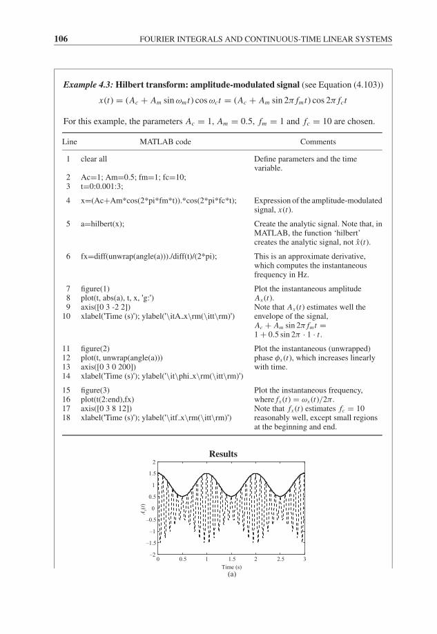
JWBK207-04 JWBK207-Shin January 18, 2008 9:1 Char Count= 0
106 FOURIER INTEGRALS AND CONTINUOUS-TIME LINEAR SYSTEMS
Example 4.3: Hilbert transform: amplitude-modulated signal (see Equation (4.103))
x(t) = (Ac + Am sin ωmt) cos ωct = (Ac + Am sin 2π fmt) cos 2π fct
For this example, the parameters Ac = 1, Am = 0.5, fm = 1 and fc = 10 are chosen.
Line MATLAB code Comments
1 clear all Define parameters and the timevariable.
2 Ac=1; Am=0.5; fm=1; fc=10;3 t=0:0.001:3;
4 x=(Ac+Am*cos(2*pi*fm*t)).*cos(2*pi*fc*t); Expression of the amplitude-modulatedsignal, x(t).
5 a=hilbert(x); Create the analytic signal. Note that, inMATLAB, the function ‘hilbert’creates the analytic signal, not x(t).
6 fx=diff(unwrap(angle(a)))./diff(t)/(2*pi); This is an approximate derivative,which computes the instantaneousfrequency in Hz.
789
10
figure(1)plot(t, abs(a), t, x, 'g:')axis([0 3 -2 2])xlabel('Time (s)'); ylabel('\itA x\rm(\itt\rm)')
Plot the instantaneous amplitudeAx (t).Note that Ax (t) estimates well theenvelope of the signal,Ac + Am sin 2π fmt =1 + 0.5 sin 2π · 1 · t .
11121314
figure(2)plot(t, unwrap(angle(a)))axis([0 3 0 200])xlabel('Time (s)'); ylabel('\it\phi x\rm(\itt\rm)')
Plot the instantaneous (unwrapped)phase φx (t), which increases linearlywith time.
15161718
figure(3)plot(t(2:end),fx)axis([0 3 8 12])xlabel('Time (s)'); ylabel('\itf x\rm(\itt\rm)')
Plot the instantaneous frequency,where fx (t) = ωx (t)/2π.Note that fx (t) estimates fc = 10reasonably well, except small regionsat the beginning and end.
Results
0 0.5 1 1.5 2 2.5 3–2
–1.5
–1
–0.5
0
0.5
1
1.5
2
Time (s)
Ax(
t)
(a)
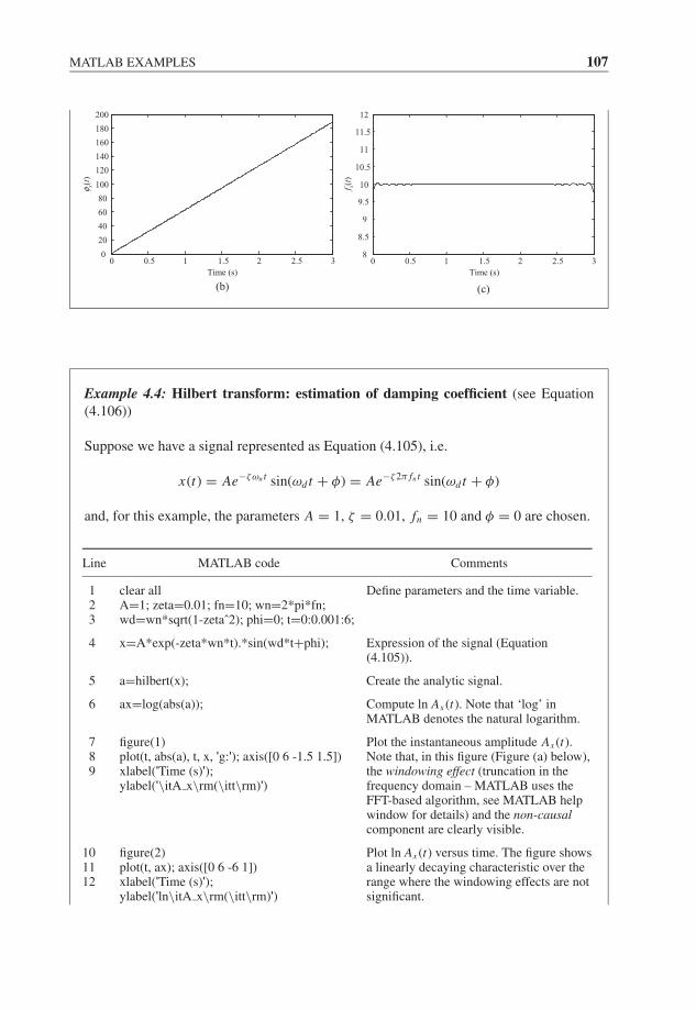
JWBK207-04 JWBK207-Shin January 18, 2008 9:1 Char Count= 0
MATLAB EXAMPLES 107
0 0.5 1 1.5 2 2.5 30
20
40
60
80
100
120
140
160
180
200
Time (s)
φ x(t)
(b)
0 0.5 1 1.5 2 2.5 38
8.5
9
9.5
10
10.5
11
11.5
12
Time (s)
f x(t)
(c)
Example 4.4: Hilbert transform: estimation of damping coefficient (see Equation(4.106))
Suppose we have a signal represented as Equation (4.105), i.e.
x(t) = Ae−ζωn t sin(ωd t + φ) = Ae−ζ2π fn t sin(ωd t + φ)
and, for this example, the parameters A = 1, ζ = 0.01, fn = 10 and φ = 0 are chosen.
Line MATLAB code Comments
1 clear all Define parameters and the time variable.2 A=1; zeta=0.01; fn=10; wn=2*pi*fn;3 wd=wn*sqrt(1-zetaˆ2); phi=0; t=0:0.001:6;
4 x=A*exp(-zeta*wn*t).*sin(wd*t+phi); Expression of the signal (Equation(4.105)).
5 a=hilbert(x); Create the analytic signal.
6 ax=log(abs(a)); Compute ln Ax (t). Note that ‘log’ inMATLAB denotes the natural logarithm.
789
figure(1)plot(t, abs(a), t, x, 'g:'); axis([0 6 -1.5 1.5])xlabel('Time (s)');ylabel('\itA x\rm(\itt\rm)')
Plot the instantaneous amplitude Ax (t).Note that, in this figure (Figure (a) below),the windowing effect (truncation in thefrequency domain – MATLAB uses theFFT-based algorithm, see MATLAB helpwindow for details) and the non-causalcomponent are clearly visible.
101112
figure(2)plot(t, ax); axis([0 6 -6 1])xlabel('Time (s)');ylabel('ln\itA x\rm(\itt\rm)')
Plot ln Ax (t) versus time. The figure showsa linearly decaying characteristic over therange where the windowing effects are notsignificant.
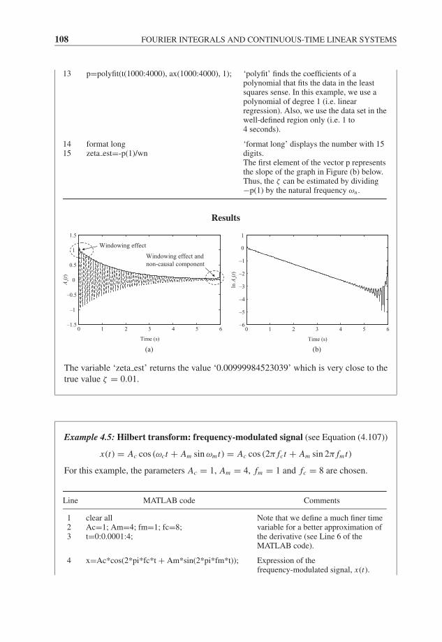
JWBK207-04 JWBK207-Shin January 18, 2008 9:1 Char Count= 0
108 FOURIER INTEGRALS AND CONTINUOUS-TIME LINEAR SYSTEMS
13 p=polyfit(t(1000:4000), ax(1000:4000), 1); ‘polyfit’ finds the coefficients of apolynomial that fits the data in the leastsquares sense. In this example, we use apolynomial of degree 1 (i.e. linearregression). Also, we use the data set in thewell-defined region only (i.e. 1 to4 seconds).
1415
format longzeta est=-p(1)/wn
‘format long’ displays the number with 15digits.The first element of the vector p representsthe slope of the graph in Figure (b) below.Thus, the ζ can be estimated by dividing−p(1) by the natural frequency ωn .
Results
lnA
x(t)
0 1 2 3 4 5 6–6
–5
–4
–3
–2
–1
0
1
Time (s)
(b)
0 1 2 3 4 5 6–1.5
–1
–0.5
0
0.5
1
1.5
Time (s)
Ax(
t)
Windowing effect
Windowing effect and
non-causal component
(a)
The variable ‘zeta est’ returns the value ‘0.00999984523039’ which is very close to thetrue value ζ = 0.01.
Example 4.5: Hilbert transform: frequency-modulated signal (see Equation (4.107))
x(t) = Ac cos (ωct + Am sin ωmt) = Ac cos (2π fct + Am sin 2π fmt)
For this example, the parameters Ac = 1, Am = 4, fm = 1 and fc = 8 are chosen.
Line MATLAB code Comments
123
clear allAc=1; Am=4; fm=1; fc=8;t=0:0.0001:4;
Note that we define a much finer timevariable for a better approximation ofthe derivative (see Line 6 of theMATLAB code).
4 x=Ac*cos(2*pi*fc*t + Am*sin(2*pi*fm*t)); Expression of thefrequency-modulated signal, x(t).
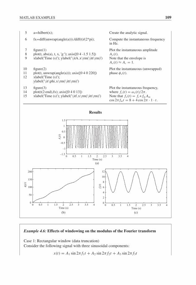
JWBK207-04 JWBK207-Shin January 18, 2008 9:1 Char Count= 0
MATLAB EXAMPLES 109
5 a=hilbert(x); Create the analytic signal.
6 fx=diff(unwrap(angle(a)))./diff(t)/(2*pi); Compute the instantaneous frequencyin Hz.
789
figure(1)plot(t, abs(a), t, x, 'g:'); axis([0 4 -1.5 1.5])xlabel('Time (s)'); ylabel('\itA x\rm(\itt\rm)')
Plot the instantaneous amplitudeAx (t).Note that the envelope isAx (t) ≈ Ac = 1.
101112
figure(2)plot(t, unwrap(angle(a))); axis([0 4 0 220])xlabel('Time (s)');ylabel('\it\phi x\rm(\itt\rm)')
Plot the instantaneous (unwrapped)phase φx (t).
131415
figure(3)plot(t(2:end),fx); axis([0 4 0 13])xlabel('Time (s)'); ylabel('\itf x\rm(\itt\rm)')
Plot the instantaneous frequency,where fx (t) = ωx (t)/2π .Note that fx (t) = fc+ fm Am
cos 2π fmt = 8 + 4 cos 2π · 1 · t .
Results
(a)
0 0.5 1 1.5 2 2.5 3 3.5 4–1.5
–1
–0.5
0
0.5
1
1.5
Time (s)
Ax(
t)
(b)
0 0.5 1 1.5 2 2.5 3 3.5 40
50
100
150
200
Time (s)
φ x(t
)
(c)
f x(t
)
0 0.5 1 1.5 2 2.5 3 3.5 40
2
4
6
8
10
12
Time (s)
Example 4.6: Effects of windowing on the modulus of the Fourier transform
Case 1: Rectangular window (data truncation)Consider the following signal with three sinusoidal components:
x(t) = A1 sin 2π f1t + A2 sin 2π f2t + A3 sin 2π f3t
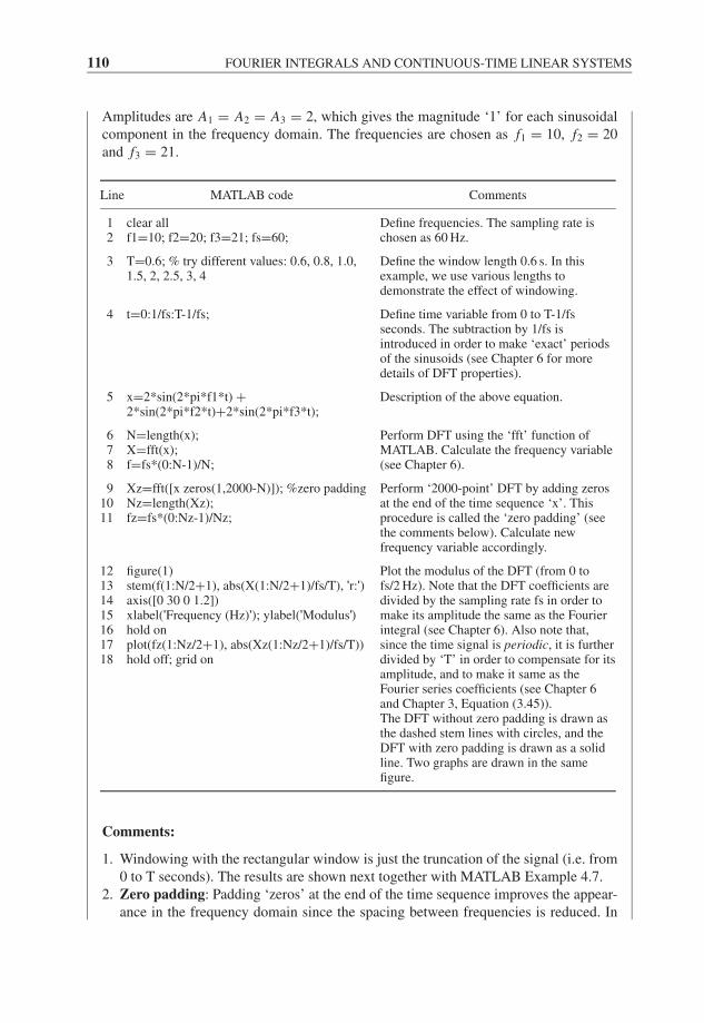
JWBK207-04 JWBK207-Shin January 18, 2008 9:1 Char Count= 0
110 FOURIER INTEGRALS AND CONTINUOUS-TIME LINEAR SYSTEMS
Amplitudes are A1 = A2 = A3 = 2, which gives the magnitude ‘1’ for each sinusoidalcomponent in the frequency domain. The frequencies are chosen as f1 = 10, f2 = 20and f3 = 21.
Line MATLAB code Comments
12
clear allf1=10; f2=20; f3=21; fs=60;
Define frequencies. The sampling rate ischosen as 60 Hz.
3 T=0.6; % try different values: 0.6, 0.8, 1.0,1.5, 2, 2.5, 3, 4
Define the window length 0.6 s. In thisexample, we use various lengths todemonstrate the effect of windowing.
4 t=0:1/fs:T-1/fs; Define time variable from 0 to T-1/fsseconds. The subtraction by 1/fs isintroduced in order to make ‘exact’ periodsof the sinusoids (see Chapter 6 for moredetails of DFT properties).
5 x=2*sin(2*pi*f1*t) +2*sin(2*pi*f2*t)+2*sin(2*pi*f3*t);
Description of the above equation.
678
N=length(x);X=fft(x);f=fs*(0:N-1)/N;
Perform DFT using the ‘fft’ function ofMATLAB. Calculate the frequency variable(see Chapter 6).
91011
Xz=fft([x zeros(1,2000-N)]); %zero paddingNz=length(Xz);fz=fs*(0:Nz-1)/Nz;
Perform ‘2000-point’ DFT by adding zerosat the end of the time sequence ‘x’. Thisprocedure is called the ‘zero padding’ (seethe comments below). Calculate newfrequency variable accordingly.
12131415161718
figure(1)stem(f(1:N/2+1), abs(X(1:N/2+1)/fs/T), 'r:')axis([0 30 0 1.2])xlabel('Frequency (Hz)'); ylabel('Modulus')hold onplot(fz(1:Nz/2+1), abs(Xz(1:Nz/2+1)/fs/T))hold off; grid on
Plot the modulus of the DFT (from 0 tofs/2 Hz). Note that the DFT coefficients aredivided by the sampling rate fs in order tomake its amplitude the same as the Fourierintegral (see Chapter 6). Also note that,since the time signal is periodic, it is furtherdivided by ‘T’ in order to compensate for itsamplitude, and to make it same as theFourier series coefficients (see Chapter 6and Chapter 3, Equation (3.45)).The DFT without zero padding is drawn asthe dashed stem lines with circles, and theDFT with zero padding is drawn as a solidline. Two graphs are drawn in the samefigure.
Comments:
1. Windowing with the rectangular window is just the truncation of the signal (i.e. from0 to T seconds). The results are shown next together with MATLAB Example 4.7.
2. Zero padding: Padding ‘zeros’ at the end of the time sequence improves the appear-ance in the frequency domain since the spacing between frequencies is reduced. In
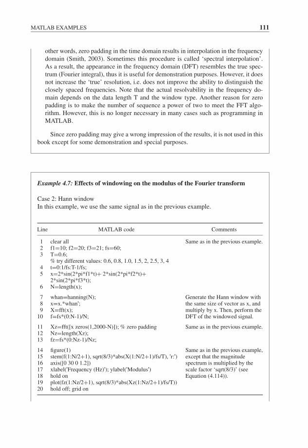
JWBK207-04 JWBK207-Shin January 18, 2008 9:1 Char Count= 0
MATLAB EXAMPLES 111
other words, zero padding in the time domain results in interpolation in the frequencydomain (Smith, 2003). Sometimes this procedure is called ‘spectral interpolation’.As a result, the appearance in the frequency domain (DFT) resembles the true spec-trum (Fourier integral), thus it is useful for demonstration purposes. However, it doesnot increase the ‘true’ resolution, i.e. does not improve the ability to distinguish theclosely spaced frequencies. Note that the actual resolvability in the frequency do-main depends on the data length T and the window type. Another reason for zeropadding is to make the number of sequence a power of two to meet the FFT algo-rithm. However, this is no longer necessary in many cases such as programming inMATLAB.
Since zero padding may give a wrong impression of the results, it is not used in thisbook except for some demonstration and special purposes.
Example 4.7: Effects of windowing on the modulus of the Fourier transform
Case 2: Hann windowIn this example, we use the same signal as in the previous example.
Line MATLAB code Comments
1 clear all Same as in the previous example.2 f1=10; f2=20; f3=21; fs=60;3 T=0.6;
% try different values: 0.6, 0.8, 1.0, 1.5, 2, 2.5, 3, 44 t=0:1/fs:T-1/fs;5 x=2*sin(2*pi*f1*t)+ 2*sin(2*pi*f2*t)+
2*sin(2*pi*f3*t);6 N=length(x);
7 whan=hanning(N); Generate the Hann window withthe same size of vector as x, andmultiply by x. Then, perform theDFT of the windowed signal.
8 x=x.*whan';9 X=fft(x);
10 f=fs*(0:N-1)/N;
11 Xz=fft([x zeros(1,2000-N)]); % zero padding Same as in the previous example.12 Nz=length(Xz);13 fz=fs*(0:Nz-1)/Nz;
14 figure(1) Same as in the previous example,except that the magnitudespectrum is multiplied by thescale factor ‘sqrt(8/3)’ (seeEquation (4.114)).
15 stem(f(1:N/2+1), sqrt(8/3)*abs(X(1:N/2+1)/fs/T), 'r:')16 axis([0 30 0 1.2])17 xlabel('Frequency (Hz)'); ylabel('Modulus')18 hold on19 plot(fz(1:Nz/2+1), sqrt(8/3)*abs(Xz(1:Nz/2+1)/fs/T))20 hold off; grid on
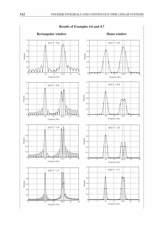
JWBK207-04 JWBK207-Shin January 18, 2008 9:1 Char Count= 0
112 FOURIER INTEGRALS AND CONTINUOUS-TIME LINEAR SYSTEMS
Results of Examples 4.6 and 4.7
Rectangular window Hann window
0 5 10 15 20 25 30210
0.2
0.4
0.6
0.8
1
1.2
Frequency (Hz)
Mo
dulu
s
(a1) T = 0.6
0 5 10 15 20 25 30210
0.2
0.4
0.6
0.8
1
1.2
Frequency (Hz)
Mo
dulu
s
(a2) T = 0.8
0 5 10 15 20 25 30210
0.2
0.4
0.6
0.8
1
1.2
Frequency (Hz)
Mo
dulu
s
(a3) T = 1.0
0 5 10 15 20 25 30210
0.2
0.4
0.6
0.8
1
1.2
Frequency (Hz)
Mo
dulu
s
(a4) T = 1.5
0 5 10 15 20 25 30210
0.2
0.4
0.6
0.8
1
1.2
Frequency (Hz)
Mo
dulu
s
(b1) T = 0.6
0 5 10 15 20 25 30210
0.2
0.4
0.6
0.8
1
1.2
Frequency (Hz)
Mo
dulu
s(b2) T = 0.8
0 5 10 15 20 25 30210
0.2
0.4
0.6
0.8
1
1.2
Frequency (Hz)
Mo
dulu
s
(b3) T = 1.0
0 5 10 15 20 25 30210
0.2
0.4
0.6
0.8
1
1.2
Frequency (Hz)
Mo
dulu
s
(b4) T = 1.5
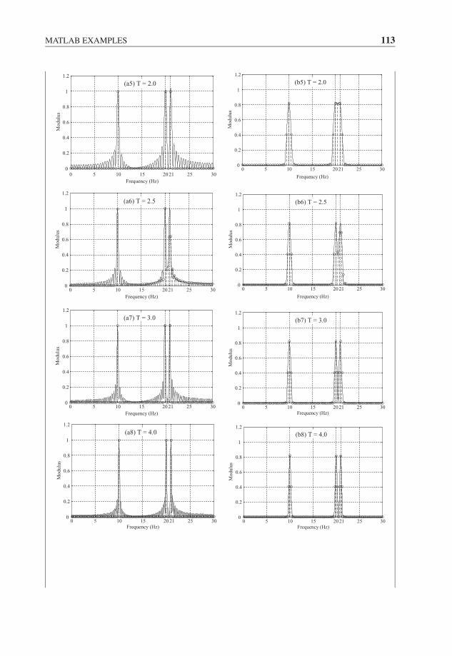
JWBK207-04 JWBK207-Shin January 18, 2008 9:1 Char Count= 0
MATLAB EXAMPLES 113
0 5 10 15 20 25 30210
0.2
0.4
0.6
0.8
1
1.2
Frequency (Hz)
Mo
dulu
s
(a5) T = 2.0
0 5 10 15 20 25 30210
0.2
0.4
0.6
0.8
1
1.2
Frequency (Hz)
Mo
dulu
s
0 5 10 15 20 25 30210
0.2
0.4
0.6
0.8
1
1.2
Frequency (Hz)
Mo
dulu
s
0 5 10 15 20 25 30210
0.2
0.4
0.6
0.8
1
1.2
Frequency (Hz)
Mo
dulu
s
0 5 10 15 20 25 30210
0.2
0.4
0.6
0.8
1
1.2
Frequency (Hz)
Mo
dulu
s
0 5 10 15 20 25 30210
0.2
0.4
0.6
0.8
1
1.2
Frequency (Hz)
Mo
dulu
s
0 5 10 15 20 25 30210
0.2
0.4
0.6
0.8
1
1.2
Frequency (Hz)
Mo
dulu
s
0 5 10 15 20 25 30210
0.2
0.4
0.6
0.8
1
1.2
Frequency (Hz)
Mo
dulu
s
(b5) T = 2.0
(b6) T = 2.5
(b7) T = 3.0
(b8) T = 4.0(a8) T = 4.0
(a7) T = 3.0
(a6) T = 2.5
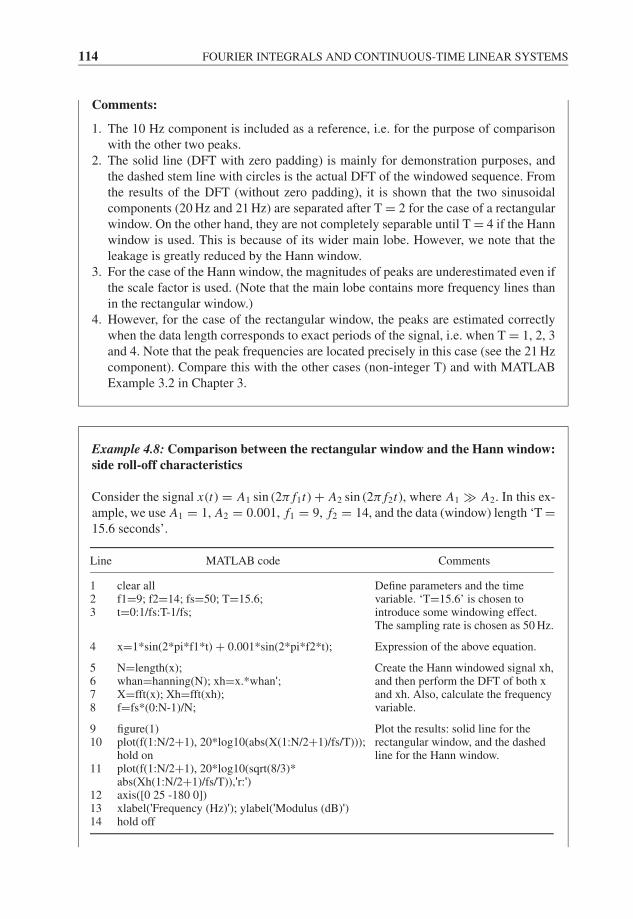
JWBK207-04 JWBK207-Shin January 18, 2008 9:1 Char Count= 0
114 FOURIER INTEGRALS AND CONTINUOUS-TIME LINEAR SYSTEMS
Comments:
1. The 10 Hz component is included as a reference, i.e. for the purpose of comparisonwith the other two peaks.
2. The solid line (DFT with zero padding) is mainly for demonstration purposes, andthe dashed stem line with circles is the actual DFT of the windowed sequence. Fromthe results of the DFT (without zero padding), it is shown that the two sinusoidalcomponents (20 Hz and 21 Hz) are separated after T = 2 for the case of a rectangularwindow. On the other hand, they are not completely separable until T = 4 if the Hannwindow is used. This is because of its wider main lobe. However, we note that theleakage is greatly reduced by the Hann window.
3. For the case of the Hann window, the magnitudes of peaks are underestimated even ifthe scale factor is used. (Note that the main lobe contains more frequency lines thanin the rectangular window.)
4. However, for the case of the rectangular window, the peaks are estimated correctlywhen the data length corresponds to exact periods of the signal, i.e. when T = 1, 2, 3and 4. Note that the peak frequencies are located precisely in this case (see the 21 Hzcomponent). Compare this with the other cases (non-integer T) and with MATLABExample 3.2 in Chapter 3.
Example 4.8: Comparison between the rectangular window and the Hann window:side roll-off characteristics
Consider the signal x(t) = A1 sin (2π f1t) + A2 sin (2π f2t), where A1 � A2. In this ex-ample, we use A1 = 1, A2 = 0.001, f1 = 9, f2 = 14, and the data (window) length ‘T =15.6 seconds’.
Line MATLAB code Comments
1 clear all Define parameters and the timevariable. ‘T=15.6’ is chosen tointroduce some windowing effect.The sampling rate is chosen as 50 Hz.
2 f1=9; f2=14; fs=50; T=15.6;3 t=0:1/fs:T-1/fs;
4 x=1*sin(2*pi*f1*t) + 0.001*sin(2*pi*f2*t); Expression of the above equation.
5 N=length(x); Create the Hann windowed signal xh,and then perform the DFT of both xand xh. Also, calculate the frequencyvariable.
6 whan=hanning(N); xh=x.*whan';7 X=fft(x); Xh=fft(xh);8 f=fs*(0:N-1)/N;
9 figure(1) Plot the results: solid line for therectangular window, and the dashedline for the Hann window.
10 plot(f(1:N/2+1), 20*log10(abs(X(1:N/2+1)/fs/T)));hold on
11 plot(f(1:N/2+1), 20*log10(sqrt(8/3)*abs(Xh(1:N/2+1)/fs/T)),'r:')
12 axis([0 25 -180 0])13 xlabel('Frequency (Hz)'); ylabel('Modulus (dB)')14 hold off
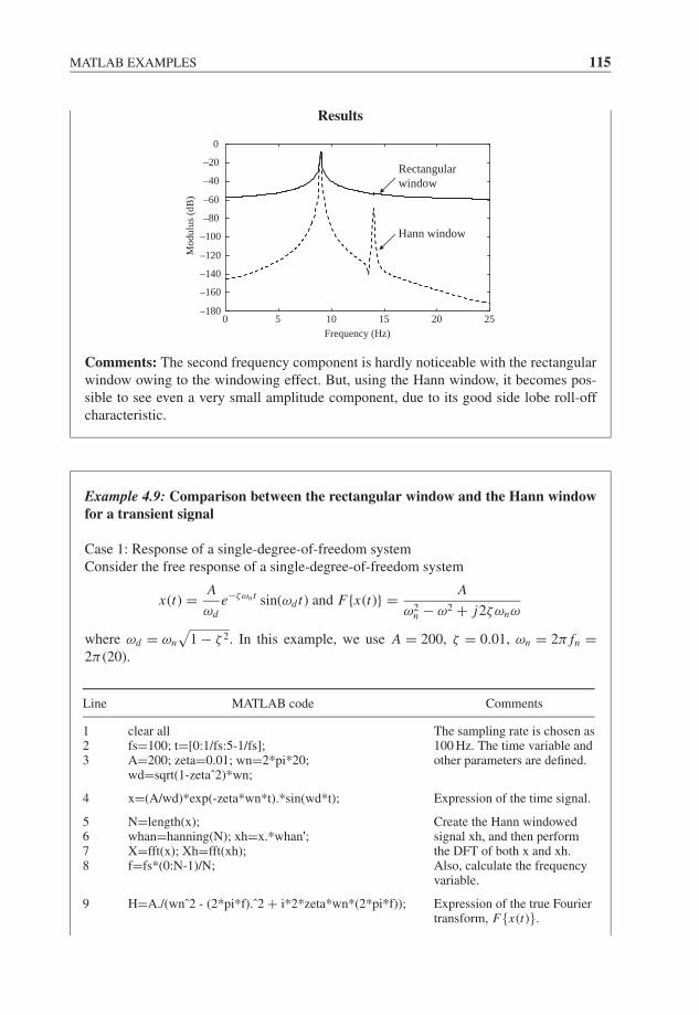
JWBK207-04 JWBK207-Shin January 18, 2008 9:1 Char Count= 0
MATLAB EXAMPLES 115
Results
0 5 10 15 20 25–180
–160
–140
–120
–100
–80
–60
–40
–20
0
Frequency (Hz)
Mod
ulus
(dB
)
Hann window
Rectangular window
Comments: The second frequency component is hardly noticeable with the rectangularwindow owing to the windowing effect. But, using the Hann window, it becomes pos-sible to see even a very small amplitude component, due to its good side lobe roll-offcharacteristic.
Example 4.9: Comparison between the rectangular window and the Hann windowfor a transient signal
Case 1: Response of a single-degree-of-freedom systemConsider the free response of a single-degree-of-freedom system
x(t) = A
ωde−ζωn t sin(ωd t) and F{x(t)} = A
ω2n − ω2 + j2ζωnω
where ωd = ωn
√1 − ζ 2. In this example, we use A = 200, ζ = 0.01, ωn = 2π fn =
2π (20).
Line MATLAB code Comments
1 clear all The sampling rate is chosen as100 Hz. The time variable andother parameters are defined.
2 fs=100; t=[0:1/fs:5-1/fs];3 A=200; zeta=0.01; wn=2*pi*20;
wd=sqrt(1-zetaˆ2)*wn;
4 x=(A/wd)*exp(-zeta*wn*t).*sin(wd*t); Expression of the time signal.
5 N=length(x); Create the Hann windowedsignal xh, and then performthe DFT of both x and xh.Also, calculate the frequencyvariable.
6 whan=hanning(N); xh=x.*whan';7 X=fft(x); Xh=fft(xh);8 f=fs*(0:N-1)/N;
9 H=A./(wnˆ2 - (2*pi*f).ˆ2 + i*2*zeta*wn*(2*pi*f)); Expression of the true Fouriertransform, F{x(t)}.
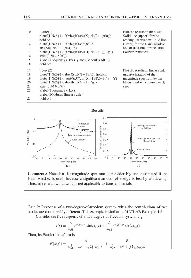
JWBK207-04 JWBK207-Shin January 18, 2008 9:1 Char Count= 0
116 FOURIER INTEGRALS AND CONTINUOUS-TIME LINEAR SYSTEMS
10 figure(1) Plot the results in dB scale:Solid line (upper) for therectangular window, solid line(lower) for the Hann window,and dashed line for the ‘true’Fourier transform.
11 plot(f(1:N/2+1), 20*log10(abs(X(1:N/2+1)/fs)));hold on
12 plot(f(1:N/2+1), 20*log10(sqrt(8/3)*abs(Xh(1:N/2+1)/fs)), 'r')
13 plot(f(1:N/2+1), 20*log10(abs(H(1:N/2+1))), 'g:')14 axis([0 50 -150 0])15 xlabel('Frequency (Hz)'); ylabel('Modulus (dB)')16 hold off
17 figure(2) Plot the results in linear scale:underestimation of themagnitude spectrum by theHann window is more clearlyseen.
18 plot(f(1:N/2+1), abs(X(1:N/2+1)/fs)); hold on19 plot(f(1:N/2+1), (sqrt(8/3)*abs(Xh(1:N/2+1)/fs)), 'r')20 plot(f(1:N/2+1), abs(H(1:N/2+1)), 'g:')21 axis([0 50 0 0.7])22 xlabel('Frequency (Hz)');
ylabel('Modulus (linear scale)')23 hold off
Results
0 5 10 15 20 25 30 35 40 45 50–150
–100
–50
0
Frequency (Hz)
Mod
ulus
(dB
)
Hann window
Rectangular window
True magnitude spectrum
(a) (b)
Hann window
Rectangular window(solid line)
True magnitude spectrum(dashed line)
0 5 10 15 20 25 30 35 40 50450
0.1
0.2
0.3
0.4
0.5
0.6
0.7
Frequency (Hz)
Mod
ulus
(lin
ear
scal
e)
Comments: Note that the magnitude spectrum is considerably underestimated if theHann window is used, because a significant amount of energy is lost by windowing.Thus, in general, windowing is not applicable to transient signals.
Case 2: Response of a two-degree-of-freedom system, when the contributions of twomodes are considerably different. This example is similar to MATLAB Example 4.8.
Consider the free response of a two-degree-of-freedom system, e.g.
x(t) = A
ωd1
e−ζ1ωn1t sin(ωd1t) + B
ωd2
e−ζ2ωn2t sin(ωd2t)
Then, its Fourier transform is
F{x(t)} = A
ω2n1 − ω2 + j2ζ1ωn1ω
+ B
ω2n2 − ω2 + j2ζ2ωn2ω

JWBK207-04 JWBK207-Shin January 18, 2008 9:1 Char Count= 0
MATLAB EXAMPLES 117
In this example, we use A = 200, B = 0.001A, ζ1 = ζ2 = 0.01, ωn1 = 2π (20) and ωn2 =2π (30). Note that A � B.
Line MATLAB code Comments
1 clear all Same as Case 1, except that theparameters for the second modeare also defined.
2 fs=100; t=[0:1/fs:5-1/fs];3 A=200; B=0.001*A; zeta1=0.01; zeta2=0.01;4 wn1=2*pi*20; wd1=sqrt(1-zeta1ˆ2)*wn1;5 wn2=2*pi*30; wd2=sqrt(1-zeta2ˆ2)*wn2;
6 x=(A/wd1)*exp(-zeta1*wn1*t).*sin(wd1*t) +(B/wd2)*exp(-zeta2*wn2*t).*sin(wd2*t);
Expression of the time signal, x(t).
7 N=length(x); Same as Case 1.8 whan=hanning(N); xh=x.*whan';9 X=fft(x); Xh=fft(xh);
10 f=fs*(0:N-1)/N;
11 H=A./(wn1ˆ2-(2*pi*f).ˆ2+i*2*zeta1*wn1*(2*pi*f))+ B./(wn2ˆ2-(2*pi*f).ˆ2+i*2*zeta2*wn2*(2*pi*f));
Expression of the true Fouriertransform, F{x(t)}.
12 figure(1) Plot the results of the rectangularwindow in dB scale: solid line forthe rectangular window anddashed line for the 'true' Fouriertransform.
13 plot(f(1:N/2+1), 20*log10(abs(X(1:N/2+1)/fs)));hold on
14 plot(f(1:N/2+1), 20*log10(abs(H(1:N/2+1))), 'g:')15 axis([0 50 -60 0])16 xlabel('Frequency (Hz)'); ylabel('Modulus (dB)')17 hold off
18 figure(2) Plot the results of the Hannwindow in dB scale: solid line forthe Hann window, and dashed linefor the ‘true’ Fourier transform.
19 plot(f(1:N/2+1), 20*log10(sqrt(8/3)*abs(Xh(1:N/2+1)/fs)))
20 hold on21 plot(f(1:N/2+1), 20*log10(abs(H(1:N/2+1))), 'g:')22 axis([0 50 -160 0])23 xlabel('Frequency (Hz)'); ylabel('Modulus (dB)')24 hold off
Results
Rectangular window
True magnitude
spectrum
0 5 10 15 20 25 30 35 40 45 50–60
–50
–40
–30
–20
–10
0
Frequency (Hz)
Mo
dulu
s (d
B)
(b) Results of the Hann window(a) Results of the rectangular window
0 5 10 15 20 25 30 35 40 45 50–160
–140
–120
–100
–80
–60
–40
–20
0
Frequency (Hz)
Mo
dulu
s (d
B)
True magnitude spectrum
Hann window
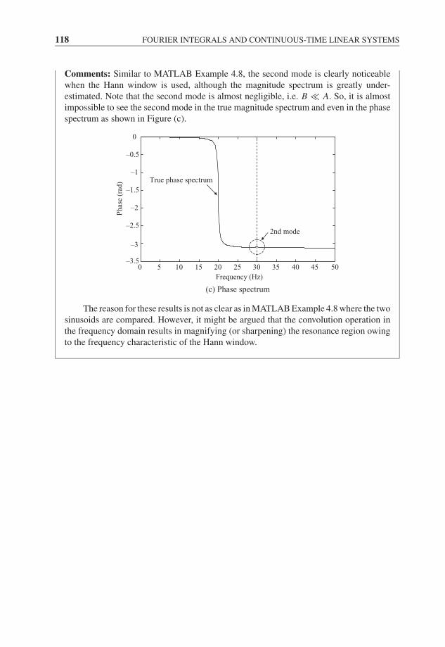
JWBK207-04 JWBK207-Shin January 18, 2008 9:1 Char Count= 0
118 FOURIER INTEGRALS AND CONTINUOUS-TIME LINEAR SYSTEMS
Comments: Similar to MATLAB Example 4.8, the second mode is clearly noticeablewhen the Hann window is used, although the magnitude spectrum is greatly under-estimated. Note that the second mode is almost negligible, i.e. B A. So, it is almostimpossible to see the second mode in the true magnitude spectrum and even in the phasespectrum as shown in Figure (c).
0 5 10 15 20 25 30 35 40 5045–3.5
–3
–2.5
–2
–1.5
–1
–0.5
0
Frequency (Hz)
(c) Phase spectrum
Phas
e (r
ad)
2nd mode
True phase spectrum
The reason for these results is not as clear as in MATLAB Example 4.8 where the twosinusoids are compared. However, it might be argued that the convolution operation inthe frequency domain results in magnifying (or sharpening) the resonance region owingto the frequency characteristic of the Hann window.
JWBK207-05 JWBK207-Shin January 26, 2008 17:5 Char Count= 0
5Time Sampling and Aliasing
Introduction
So far, we have developed the Fourier transform of a continuous signal. However, we usuallyutilize a digital computer to perform the transform. Thus, it is necessary to re-examine Fouriermethods so as to be able to transform sampled data. We would ‘hope’ that the discrete versionof the Fourier transform resembles (or approximates) the Fourier integral (Equation (4.6)),such that it represents the frequency characteristic (within the range of interest) of the originalsignal. In fact, from the MATLAB examples given in the previous chapter, we have alreadyseen that the results of the discrete version (DFT) and the continuous version (Fourier integral)appear to be not very different. However, there are fundamental differences between these twoversions, and in this chapter we shall consider the effect of sampling, and relate the Fouriertransform of a continuous signal and the transform of a discrete signal (or a sequence).
5.1 THE FOURIER TRANSFORM OF AN IDEALSAMPLED SIGNAL
Impulse Train Modulation
We introduce the Fourier transform of a sequence by using the mathematical notion of‘ideal sampling’ of a continuous signal. Consider a ‘train’ of delta functions i(t) whichis expressed as
i(t) =∞∑
n=−∞δ(t − n�) (5.1)
Fundamentals of Signal Processing for Sound and Vibration EngineersK. Shin and J. K. Hammond. C© 2008 John Wiley & Sons, Ltd
119
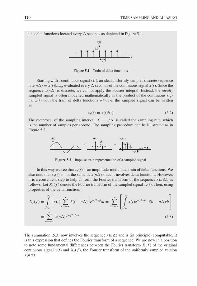
JWBK207-05 JWBK207-Shin January 26, 2008 17:5 Char Count= 0
120 TIME SAMPLING AND ALIASING
i.e. delta functions located every � seconds as depicted in Figure 5.1.
1.0
Δ
. . .. . .
i(t)
t
Figure 5.1 Train of delta functions
Starting with a continuous signal x(t), an ideal uniformly sampled discrete sequenceis x(n�) = x(t)|t=n� evaluated every � seconds of the continuous signal x(t). Since thesequence x(n�) is discrete, we cannot apply the Fourier integral. Instead, the ideallysampled signal is often modelled mathematically as the product of the continuous sig-nal x(t) with the train of delta functions i(t), i.e. the sampled signal can be writtenas
xs(t) = x(t)i(t) (5.2)
The reciprocal of the sampling interval, fs = 1/�, is called the sampling rate, whichis the number of samples per second. The sampling procedure can be illustrated as inFigure 5.2.
( )sx t
=×Δ
... ...
( )i t( )tx
Figure 5.2 Impulse train representation of a sampled signal
In this way we see that xs(t) is an amplitude-modulated train of delta functions. Wealso note that xs(t) is not the same as x(n�) since it involves delta functions. However,it is a convenient step to help us form the Fourier transform of the sequence x(n�), asfollows. Let Xs( f ) denote the Fourier transform of the sampled signal xs(t). Then, usingproperties of the delta function,
Xs( f ) =∞∫
−∞
[x(t)
∞∑n=−∞
δ(t − n�)
]e− j2π ftdt =
∞∑n=−∞
⎡⎣ ∞∫−∞
x(t)e− j2π ft · δ(t − n�)dt
⎤⎦=
∞∑n=−∞
x(n�)e− j2π fn� (5.3)
The summation (5.3) now involves the sequence x(n�) and is (in principle) computable. Itis this expression that defines the Fourier transform of a sequence. We are now in a positionto note some fundamental differences between the Fourier transform X ( f ) of the originalcontinuous signal x(t) and Xs( f ), the Fourier transform of the uniformly sampled versionx(n�).
JWBK207-05 JWBK207-Shin January 26, 2008 17:5 Char Count= 0
THE FOURIER TRANSFORM OF AN IDEAL SAMPLED SIGNAL 121
Note that Equation (5.3) implies that Xs( f ) has a periodic structure in frequency withperiod 1/�. For example, for an integer number r , Xs( f + r/�) becomes
Xs( f + r/�) =∞∑
n=−∞x(n�)e− j2π ( f +r/�)n� =
∞∑n=−∞
x(n�)e− j2π fn�e− j2πrn
=∞∑
n=−∞x(n�)e− j2π fn� = Xs( f ) (5.4)
This periodicity in frequency will be discussed further shortly. The inverse Fourier transformof Xs( f ) can be found by multiplying both sides of Equation (5.3) by e j2π f r� and integratingwith respect to f from −1/2� to 1/2� (since Xs( f ) is periodic, we need to integrate overonly one period), and taking account of the orthogonality of the exponential function. Then
1/2�∫−1/2�
Xs( f )e j2π f r�df =1/2�∫
−1/2�
[ ∞∑n=−∞
x(n�)e− j2π fn�
]e j2π f r�df
=∞∑
n=−∞
⎡⎢⎣ 1/2�∫−1/2�
x(n�)e− j2π fn�e j2π f r�df
⎤⎥⎦=
∞∑n=−∞
⎡⎢⎣x(n�)
1/2�∫−1/2�
e− j2π f (n−r )�df
⎤⎥⎦ = x(r�)1
�(5.5)
Thus, we summarize the Fourier transform pair for the ‘sampled sequence’ as below,where we rename Xs( f ) as X (e j2π f �):
X (e j2π f �) =∞∑
n=−∞x(n�)e− j2π fn� (5.6)
x(n�) = �
1/2�∫−1/2�
X (e j2π f �)e j2π fn�df (5.7)
Note that the scaling factor � is present in Equation (5.7).
The Link Between X(e j2π fΔ) and X( f )
At this stage, we may ask: ‘How is the Fourier transform of a sequence X (e j2π f �) relatedto the Fourier transform of a continuous signal X ( f )?’ In order to answer this, we need toexamine the periodicity of X (e j2π f �) as follows.
Note that i(t) in Equation (5.1) is a periodic signal with period �, thus it has a Fourierseries representation. Since the fundamental period TP = �, we can write the train of delta
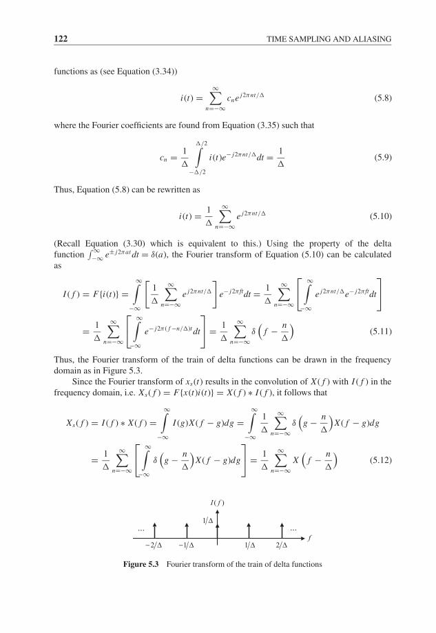
JWBK207-05 JWBK207-Shin January 26, 2008 17:5 Char Count= 0
122 TIME SAMPLING AND ALIASING
functions as (see Equation (3.34))
i(t) =∞∑
n=−∞cne j2πnt/� (5.8)
where the Fourier coefficients are found from Equation (3.35) such that
cn = 1
�
�/2∫−�/2
i(t)e− j2πnt/�dt = 1
�(5.9)
Thus, Equation (5.8) can be rewritten as
i(t) = 1
�
∞∑n=−∞
e j2πnt/� (5.10)
(Recall Equation (3.30) which is equivalent to this.) Using the property of the deltafunction
∫ ∞−∞ e± j2πat dt = δ(a), the Fourier transform of Equation (5.10) can be calculated
as
I ( f ) = F{i(t)} =∞∫
−∞
[1
�
∞∑n=−∞
e j2πnt/�
]e− j2π ftdt = 1
�
∞∑n=−∞
⎡⎣ ∞∫−∞
e j2πnt/�e− j2π ftdt
⎤⎦= 1
�
∞∑n=−∞
⎡⎣ ∞∫−∞
e− j2π ( f −n/�)t dt
⎤⎦ = 1
�
∞∑n=−∞
δ(
f − n
�
)(5.11)
Thus, the Fourier transform of the train of delta functions can be drawn in the frequencydomain as in Figure 5.3.
Since the Fourier transform of xs(t) results in the convolution of X ( f ) with I ( f ) in thefrequency domain, i.e. Xs( f ) = F{x(t)i(t)} = X ( f ) ∗ I ( f ), it follows that
Xs( f ) = I ( f ) ∗ X ( f ) =∞∫
−∞I (g)X ( f − g)dg =
∞∫−∞
1
�
∞∑n=−∞
δ(
g − n
�
)X ( f − g)dg
= 1
�
∞∑n=−∞
⎡⎣ ∞∫−∞
δ(
g − n
�
)X ( f − g)dg
⎤⎦ = 1
�
∞∑n=−∞
X(
f − n
�
)(5.12)
... ...
1 Δ
( )I f
1 Δ
2 Δ1− Δ2− Δf
Figure 5.3 Fourier transform of the train of delta functions

JWBK207-05 JWBK207-Shin January 26, 2008 17:5 Char Count= 0
THE FOURIER TRANSFORM OF AN IDEAL SAMPLED SIGNAL 123
This gives an alternative form of Equation (5.6), which is
X (e j2π f �) = 1
�
∞∑n=−∞
X(
f − n
�
)(5.13)
This important equation describes the relationship between the Fourier transform of acontinuous signal and the Fourier transform of a sequence obtained by ideal samplingevery � seconds. That is, the Fourier transform of the sequence x(n�) is the sum of shiftedversions of the Fourier transform of the underlying continuous signal. This reinforces theperiodic nature of X (e j2π f �). Note also that the ‘scaling’ effect 1/�, i.e. the samplingrate fs = 1/�, is a multiplier of the sum in Equation (5.13).
So, the ‘sampling in the time domain’ implies a ‘periodic and continuous structurein the frequency domain’ as illustrated in Figure 5.4. From Equation (5.6), it can beseen that Xs( fs − f ) = X∗
s ( f ), where * denotes complex conjugate. This is confirmed(for the modulus) from Figure 5.4. Thus, all the information in Xs( f ) lies in the range0 ≤ f ≤ fs/2. This figure emphasizes the difference between X ( f ) and X (e j2π f �), andleads to the concept of ‘aliasing’, which arises from the possible overlapping betweenthe replicas of X ( f ). This will be discussed further in the next section.
2( )j fX e π ΔΔ
1
2Δ
...
( )X f
1
Δ
...
3
2Δ
f
Aliasing
3
2−
Δ1−Δ
1
2−
Δ
Figure 5.4 Fourier transform of the sampled sequence
An Alternative Route to the Derivation of the Fourier Transformof a Sequence
The z-transform
The expression for the Fourier transform of a sequence, Equation (5.6), can also be obtainedvia the z-transform of a sequence. The z-transform is widely used in the solution of differenceequations, just as the Laplace transform is used for differential equations. The definition ofthe z-transform X(z) of a sequence of numbers x(n) is
X (z) =∞∑
n=−∞x(n)z−n (5.14)
where z is the complex-valued argument of the transform and X(z) is a function of a complexvariable. In Equation (5.14), the notion of time is not explicitly made, i.e. we write x(n) forx(n�). It is convenient here to regard the sampling interval as set to unity. Since z is complex,it can be written in polar form, i.e. using the magnitude and phase such that z = re jω, and isrepresented in a complex plane (polar coordinates) as shown in Figure 5.5(a). If this expression
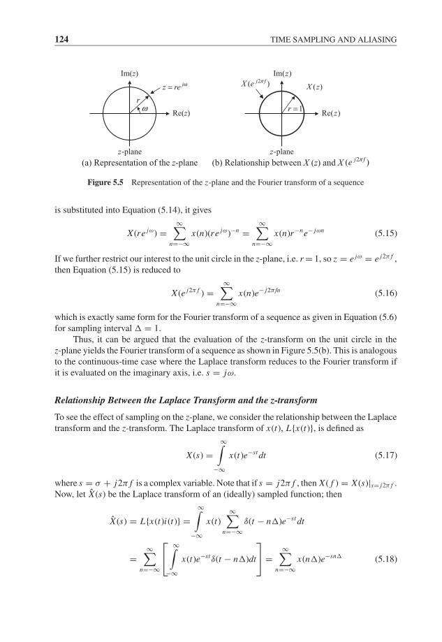
JWBK207-05 JWBK207-Shin January 26, 2008 17:5 Char Count= 0
124 TIME SAMPLING AND ALIASING
2( )j fX e πIm( )z
Re( )z1r =
( )X z
-planez
(a) Representation of the z-plane 2( )j fe π(b) Relationship between X (z) and X
jz re ω=
-planez
Re(z)
Im(z)
rω
Figure 5.5 Representation of the z-plane and the Fourier transform of a sequence
is substituted into Equation (5.14), it gives
X (re jω) =∞∑
n=−∞x(n)(re jω)−n =
∞∑n=−∞
x(n)r−ne− jωn (5.15)
If we further restrict our interest to the unit circle in the z-plane, i.e. r = 1, so z = e jω = e j2π f ,then Equation (5.15) is reduced to
X (e j2π f ) =∞∑
n=−∞x(n)e− j2π fn (5.16)
which is exactly same form for the Fourier transform of a sequence as given in Equation (5.6)for sampling interval � = 1.
Thus, it can be argued that the evaluation of the z-transform on the unit circle in thez-plane yields the Fourier transform of a sequence as shown in Figure 5.5(b). This is analogousto the continuous-time case where the Laplace transform reduces to the Fourier transform ifit is evaluated on the imaginary axis, i.e. s = jω.
Relationship Between the Laplace Transform and the z-transform
To see the effect of sampling on the z-plane, we consider the relationship between the Laplacetransform and the z-transform. The Laplace transform of x(t), L{x(t)}, is defined as
X (s) =∞∫
−∞x(t)e−st dt (5.17)
where s = σ + j2π f is a complex variable. Note that if s = j2π f , then X ( f ) = X (s)|s= j2π f .Now, let X (s) be the Laplace transform of an (ideally) sampled function; then
X (s) = L{x(t)i(t)} =∞∫
−∞x(t)
∞∑n=−∞
δ(t − n�)e−st dt
=∞∑
n=−∞
⎡⎣ ∞∫−∞
x(t)e−stδ(t − n�)dt
⎤⎦ =∞∑
n=−∞x(n�)e−sn� (5.18)
JWBK207-05 JWBK207-Shin January 26, 2008 17:5 Char Count= 0
THE FOURIER TRANSFORM OF AN IDEAL SAMPLED SIGNAL 125
If z = es�, then Equation (5.18) becomes the z-transform, i.e.
X (s)∣∣z=es� =
∞∑n=−∞
x(n�)z−n = X (z) (5.19)
Comparing Equation (5.19) with Equation (5.6), it can be shown that if z = e j2π f �, then
X (e j2π f �) = X (z)|z=e j2π f � (5.20)
Also, using the similar argument made in Equation (5.13), i.e. using
i(t) = 1
�
∞∑n=−∞
e j2πnt/�
an alternative form of X (s) can be written as
X (s) =∞∫
−∞x(t)
1
�
∞∑n=−∞
e j2πnt/�e−st dt = 1
�
∞∑n=−∞
⎡⎣ ∞∫−∞
x(t)e−(s− j2πn/�)t dt
⎤⎦ (5.21)
Thus,
X (s) = 1
�
∞∑n=−∞
X
(s − j2πn
�
)(5.22)
From Equation (5.22), we can see that X (s) is related to X (s) by adding shifted ver-sions of scaled X (s) to produce X (s) as depicted in Figure 5.6(b) below, which is similarto the relationship between the Fourier transform of a sampled sequence and the Fouriertransform.
Note that, as we can see from Equation (5.19), X (z) is not directly related to X (s), butit is related to X (s) via z = es�. Further, if we let s = j2π f , then we have the followingrelationship:
Xs( f )(= X (e j2π f �)
) = X (s)∣∣s= j2π f = X (z)|z=e j2π f � (5.23)
The relationships between X (s), X (s) and X (z) are illustrated in Figure 5.6. In this figure, apole is included in the s-plane to demonstrate how it is mapped to the z-plane. We can seethat a single pole in the X (s)-plane results in an infinite number of poles in the X (s)-plane;then this infinite series of poles all map onto a single pole in the X (z)-plane. In effect, the lefthand side of the s-plane is mapped to the inside of the unit circle of the z-plane. However, wemust realize that, due to the sampling process, what it maps onto the z-plane is not X (s), butX (s), and each ‘strip’ in the left hand side of X (s) is mapped onto the z-plane plane such thatit fills the complete unit circle. This indicates the ‘periodic’ structure in the frequency domainas well as possible aliasing in the frequency domain.
The above mapping process is sometimes used in designing an IIR (Infinite ImpulseResponse) digital filter from an existing analogue filter, and is called the impulse-invariantmethod.
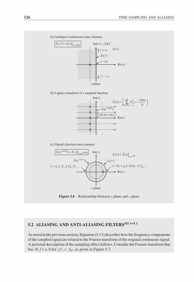
JWBK207-05 JWBK207-Shin January 26, 2008 17:5 Char Count= 0
126 TIME SAMPLING AND ALIASING
(c) Digital (discrete-time) domain:
-planez
1z =0, ( 1 ) , 2 ,s sf f f= ± = Δ ± ...2 , 3 2,s sf f f= ± ± ...
2( )j fX e π Δ
ˆ( ) ( ) sz eX z X s Δ=
=Im( )z
Re( )z
22( ) ( )j f
j fz eX e X zππ
ΔΔ==
(a) Analogue (continuous-time) domain:
( )X f
0f =
( )X s
Im( ) 2s j fπ=
Re( )s
f = ∞
f = −∞
-planes
2( ) ( ) s j fX f X s π==
Im( )s
Re( )s
1 2ˆ ( )n=−∞
j nX s X s
π∞ ⎛ ⎞= −⎜ ⎟Δ Δ⎝ ⎠∑
( )2 2 sfπ πΔ =
2( )j fX e π Δ
......
(b) Laplace transform of a sampled function:
Figure 5.6 Relationship between s-plane and z-plane
5.2 ALIASING AND ANTI-ALIASING FILTERSM5.1–5.3
As noted in the previous section, Equation (5.13) describes how the frequency componentsof the sampled signal are related to the Fourier transform of the original continuous signal.A pictorial description of the sampling effect follows. Consider the Fourier transform thathas X ( f ) = 0 for | f | > fH , as given in Figure 5.7.
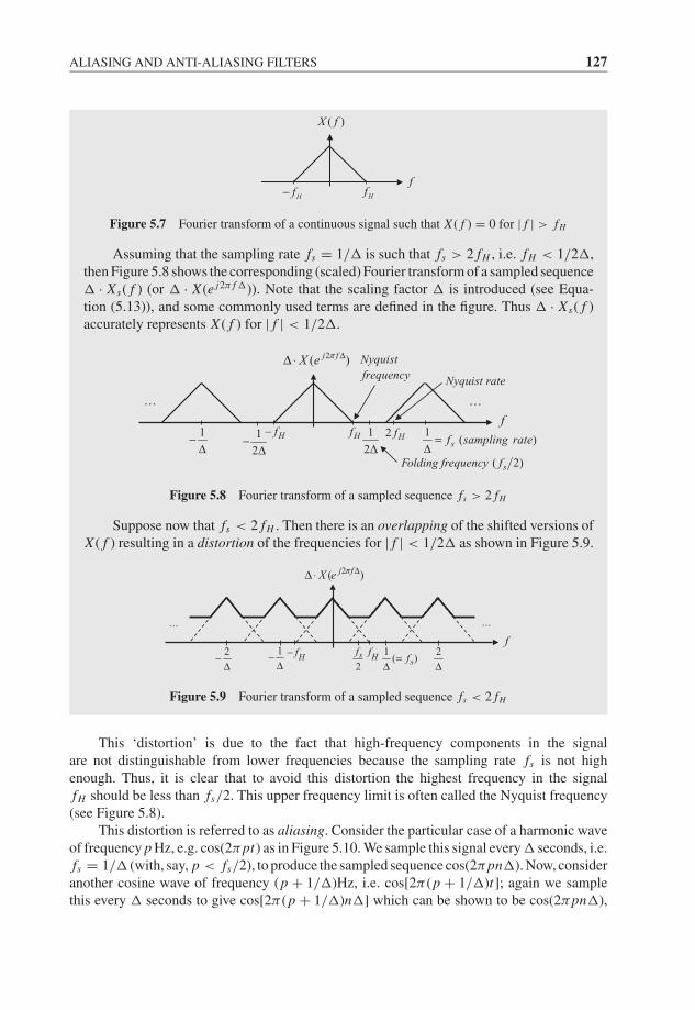
JWBK207-05 JWBK207-Shin January 26, 2008 17:5 Char Count= 0
ALIASING AND ANTI-ALIASING FILTERS 127
Hf
( )X f
Hf−f
Figure 5.7 Fourier transform of a continuous signal such that X ( f ) = 0 for | f | > fH
Assuming that the sampling rate fs = 1/� is such that fs > 2 fH , i.e. fH < 1/2�,then Figure 5.8 shows the corresponding (scaled) Fourier transform of a sampled sequence� · Xs( f ) (or � · X (e j2π f �)). Note that the scaling factor � is introduced (see Equa-tion (5.13)), and some commonly used terms are defined in the figure. Thus � · Xs( f )accurately represents X ( f ) for | f | < 1/2�.
Hf
2( )j fX e π ΔΔ ⋅
Hf− 1
2Δ1
( )sf sampling rate=Δ
1
2−
Δ1−Δ
2 Hf
( 2)sFolding frequency f
......
Nyquist rate
Nyquist frequency
f
Figure 5.8 Fourier transform of a sampled sequence fs > 2 fH
Suppose now that fs < 2 fH . Then there is an overlapping of the shifted versions ofX ( f ) resulting in a distortion of the frequencies for | f | < 1/2� as shown in Figure 5.9.
HfHf− 1( )sf=
Δ1−Δ
2−Δ
... ...
2sf
2( )j fX e π ΔΔ ⋅
f2
Δ
Figure 5.9 Fourier transform of a sampled sequence fs < 2 fH
This ‘distortion’ is due to the fact that high-frequency components in the signalare not distinguishable from lower frequencies because the sampling rate fs is not highenough. Thus, it is clear that to avoid this distortion the highest frequency in the signalfH should be less than fs/2. This upper frequency limit is often called the Nyquist frequency(see Figure 5.8).
This distortion is referred to as aliasing. Consider the particular case of a harmonic waveof frequency p Hz, e.g. cos(2πpt) as in Figure 5.10. We sample this signal every � seconds, i.e.fs = 1/� (with, say, p < fs/2), to produce the sampled sequence cos(2πpn�). Now, consideranother cosine wave of frequency (p + 1/�)Hz, i.e. cos[2π (p + 1/�)t]; again we samplethis every � seconds to give cos[2π (p + 1/�)n�] which can be shown to be cos(2πpn�),
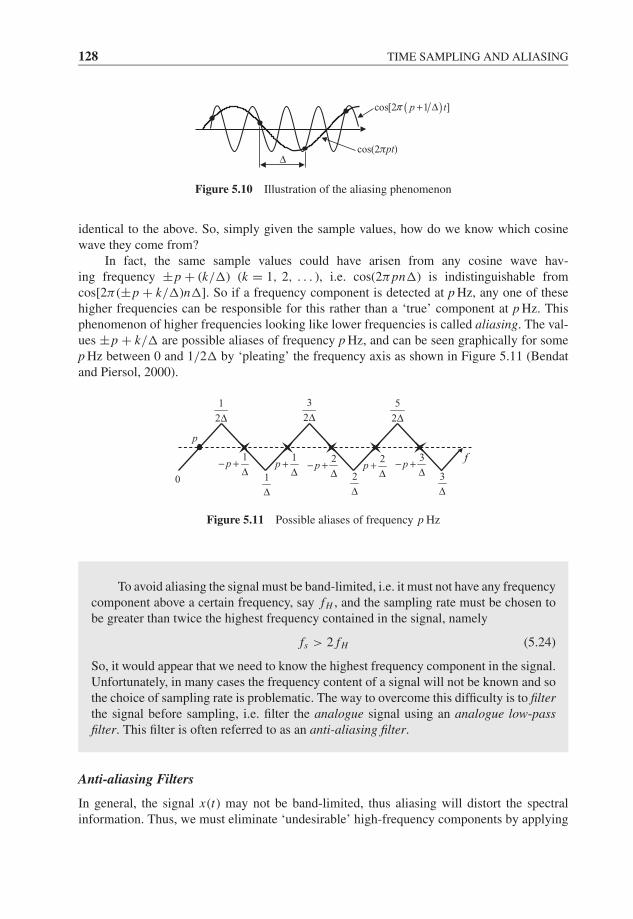
JWBK207-05 JWBK207-Shin January 26, 2008 17:5 Char Count= 0
128 TIME SAMPLING AND ALIASING
cos(2πpt)
( )cos[2 ]1p tπ + Δ
Δ
Figure 5.10 Illustration of the aliasing phenomenon
identical to the above. So, simply given the sample values, how do we know which cosinewave they come from?
In fact, the same sample values could have arisen from any cosine wave hav-ing frequency ±p + (k/�) (k = 1, 2, . . . ), i.e. cos(2πpn�) is indistinguishable fromcos[2π (±p + k/�)n�]. So if a frequency component is detected at p Hz, any one of thesehigher frequencies can be responsible for this rather than a ‘true’ component at p Hz. Thisphenomenon of higher frequencies looking like lower frequencies is called aliasing. The val-ues ±p + k/� are possible aliases of frequency p Hz, and can be seen graphically for somep Hz between 0 and 1/2� by ‘pleating’ the frequency axis as shown in Figure 5.11 (Bendatand Piersol, 2000).
1
2Δ
1p− +
Δ1
Δ2
Δ
5
2Δ3
2Δ
1p +
Δ2
p− +Δ
2p +
Δ3
p− +Δ
p
f
0 3
Δ
Figure 5.11 Possible aliases of frequency p Hz
To avoid aliasing the signal must be band-limited, i.e. it must not have any frequencycomponent above a certain frequency, say fH , and the sampling rate must be chosen tobe greater than twice the highest frequency contained in the signal, namely
fs > 2 fH (5.24)
So, it would appear that we need to know the highest frequency component in the signal.Unfortunately, in many cases the frequency content of a signal will not be known and sothe choice of sampling rate is problematic. The way to overcome this difficulty is to filterthe signal before sampling, i.e. filter the analogue signal using an analogue low-passfilter. This filter is often referred to as an anti-aliasing filter.
Anti-aliasing Filters
In general, the signal x(t) may not be band-limited, thus aliasing will distort the spectralinformation. Thus, we must eliminate ‘undesirable’ high-frequency components by applying
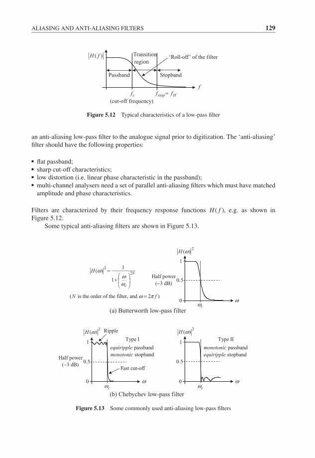
JWBK207-05 JWBK207-Shin January 26, 2008 17:5 Char Count= 0
ALIASING AND ANTI-ALIASING FILTERS 129
( )H f
cf
‘Roll-off’ of the filter
stop Hf f≈f
StopbandPassband
Transition
region
(cut-off frequency)
Figure 5.12 Typical characteristics of a low-pass filter
an anti-aliasing low-pass filter to the analogue signal prior to digitization. The ‘anti-aliasing’filter should have the following properties:� flat passband;� sharp cut-off characteristics;� low distortion (i.e. linear phase characteristic in the passband);� multi-channel analysers need a set of parallel anti-aliasing filters which must have matched
amplitude and phase characteristics.
Filters are characterized by their frequency response functions H ( f ), e.g. as shown inFigure 5.12.
Some typical anti-aliasing filters are shown in Figure 5.13.
2( )H ω
cω
2
2
1( )
1
N
c
H ωωω
=⎛ ⎞
+ ⎜ ⎟⎝ ⎠
( is the order of the filter, and 2 )
(a) Butterworth low-pass filter
(b) Chebychev low-pass filter
fN ω π=
Half power
(−3 dB)
(−3 dB)
ω0
0.5
1
2( )H ω 2
( )H ω
Half power
0
0.5
1
0
0.5
1
cω cωωω
Ripple
Fast cut-off
Type I
passband
stopband
equiripplemonotonic
Type II
passband
stopband
monotonicequiripple
Figure 5.13 Some commonly used anti-aliasing low-pass filters

JWBK207-05 JWBK207-Shin January 26, 2008 17:5 Char Count= 0
130 TIME SAMPLING AND ALIASING
We shall assume that the anti-aliasing filter operates on the signal x(t) to produce asignal to be digitized as illustrated in Figure 5.14.
Anti-aliasing filter,
H( f )ADC
x(t) x(nΔ)
Figure 5.14 The use of anti-aliasing filter prior to sampling
But we still need to decide what the highest frequency fH is just prior to the ADC(analogue-to-digital converter). The critical features in deciding this are:� the ‘cut-off’ frequency of the filter fc, usually the fc (Hz) = 3 dB point of the filter;� the ‘roll-off rate’ of the filter in dB/octave (B in Figure 5.15);� the ‘dynamic range’ of the acquisition system in dB (A in Figure 5.15). (Dynamic range
is discussed in the next section.)
These terms and the effect of sampling rate are depicted in Figure 5.15. Note that, in thisfigure, if fs > 2 fstop(≈ 2 fH ) there is no aliasing, and if fs > 2 f A there is no aliasing upto fc. Also note that it is not the 3 dB point of the filter which should satisfy the Nyquistcriterion. But at the Nyquist frequency the filter response should be negligible (e.g. atleast 40 dB down on the passband).
Hf f≈
( )H f
Afcf2
sf
( )2log in octavescf f
sf
Roll-off:
(dB octave)B
2s A cf f f f= = +
2s stop
stop
stop
stop
f f=0
Filter gain
(dB)
Passband
f
Noise floor
Dynamic range: A (dB)
Figure 5.15 Characteristics of the anti-aliasing filter
If the spectrum is to be used up to fc Hz, then the figure indicates how fs is chosen. Usingsimple trigonometry,
− A
log2( fstop/ fc)= −B (dB/octave) (5.25)
Note that if B is dB/decade, then the logarithm is to base 10. Some comments on the octaveare: if f2 = 2n f1, then f2 is ‘n’ octaves; thus, log2 f2 = n + log2 f1 and log2 f2 − log2 f1 =log2( f2/ f1) = n (octaves).
From Equation (5.25), it can be shown that fstop = 2A/B fc. Substituting this expressioninto fs > fstop + fc, which is the condition for no aliasing up to the cut-off frequency fc
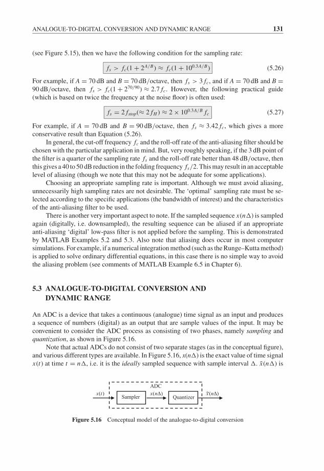
JWBK207-05 JWBK207-Shin January 26, 2008 17:5 Char Count= 0
ANALOGUE-TO-DIGITAL CONVERSION AND DYNAMIC RANGE 131
(see Figure 5.15), then we have the following condition for the sampling rate:
fs > fc(1 + 2A/B) ≈ fc(1 + 100.3A/B) (5.26)
For example, if A = 70 dB and B = 70 dB/octave, then fs > 3 fc, and if A = 70 dB and B =90 dB/octave, then fs > fc(1 + 270/90) ≈ 2.7 fc. However, the following practical guide(which is based on twice the frequency at the noise floor) is often used:
fs = 2 fstop(≈ 2 fH ) ≈ 2 × 100.3A/B fc (5.27)
For example, if A = 70 dB and B = 90 dB/octave, then fs ≈ 3.42 fc, which gives a moreconservative result than Equation (5.26).
In general, the cut-off frequency fc and the roll-off rate of the anti-aliasing filter should bechosen with the particular application in mind. But, very roughly speaking, if the 3 dB point ofthe filter is a quarter of the sampling rate fs and the roll-off rate better than 48 dB/octave, thenthis gives a 40 to 50 dB reduction in the folding frequency fs/2. This may result in an acceptablelevel of aliasing (though we note that this may not be adequate for some applications).
Choosing an appropriate sampling rate is important. Although we must avoid aliasing,unnecessarily high sampling rates are not desirable. The ‘optimal’ sampling rate must be se-lected according to the specific applications (the bandwidth of interest) and the characteristicsof the anti-aliasing filter to be used.
There is another very important aspect to note. If the sampled sequence x(n�) is sampledagain (digitally, i.e. downsampled), the resulting sequence can be aliased if an appropriateanti-aliasing ‘digital’ low-pass filter is not applied before the sampling. This is demonstratedby MATLAB Examples 5.2 and 5.3. Also note that aliasing does occur in most computersimulations. For example, if a numerical integration method (such as the Runge–Kutta method)is applied to solve ordinary differential equations, in this case there is no simple way to avoidthe aliasing problem (see comments of MATLAB Example 6.5 in Chapter 6).
5.3 ANALOGUE-TO-DIGITAL CONVERSION ANDDYNAMIC RANGE
An ADC is a device that takes a continuous (analogue) time signal as an input and producesa sequence of numbers (digital) as an output that are sample values of the input. It may beconvenient to consider the ADC process as consisting of two phases, namely sampling andquantization, as shown in Figure 5.16.
Note that actual ADCs do not consist of two separate stages (as in the conceptual figure),and various different types are available. In Figure 5.16, x(n�) is the exact value of time signalx(t) at time t = n�, i.e. it is the ideally sampled sequence with sample interval �. x(n�) is
x~(nΔ)Sampler Quantizer
( )x t ( )x nΔADC
Figure 5.16 Conceptual model of the analogue-to-digital conversion
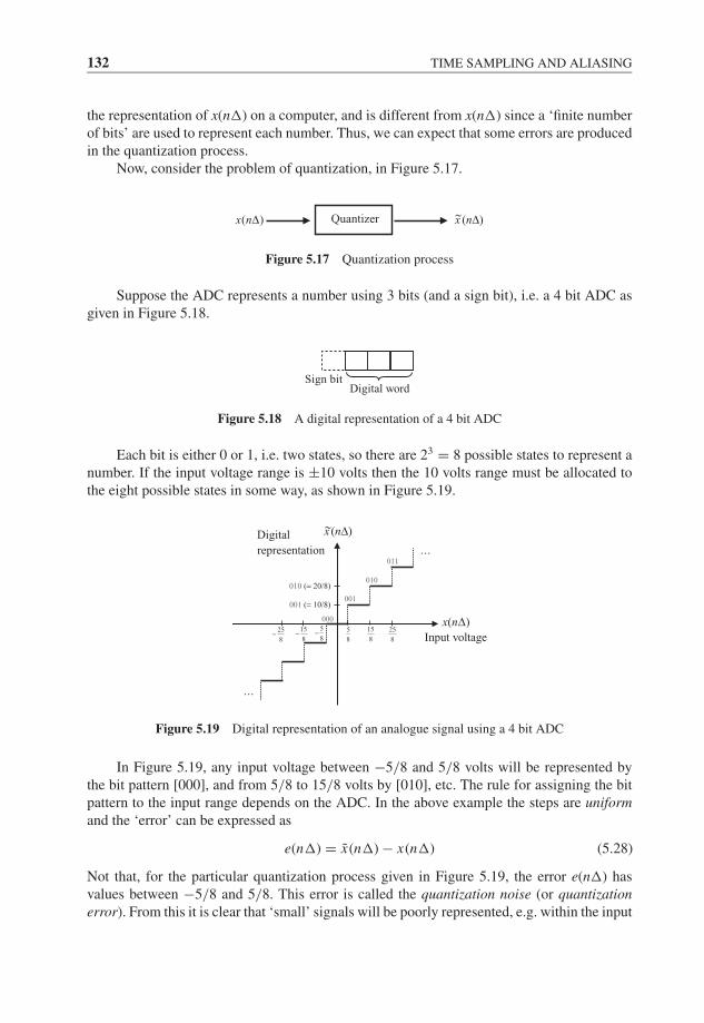
JWBK207-05 JWBK207-Shin January 26, 2008 17:5 Char Count= 0
132 TIME SAMPLING AND ALIASING
the representation of x(n�) on a computer, and is different from x(n�) since a ‘finite numberof bits’ are used to represent each number. Thus, we can expect that some errors are producedin the quantization process.
Now, consider the problem of quantization, in Figure 5.17.
x~(nΔ)Quantizer( )x nΔ
Figure 5.17 Quantization process
Suppose the ADC represents a number using 3 bits (and a sign bit), i.e. a 4 bit ADC asgiven in Figure 5.18.
Digital wordSign bit
Figure 5.18 A digital representation of a 4 bit ADC
Each bit is either 0 or 1, i.e. two states, so there are 23 = 8 possible states to represent anumber. If the input voltage range is ±10 volts then the 10 volts range must be allocated tothe eight possible states in some way, as shown in Figure 5.19.
5
8
15
8
25
8−
5
8−
001 (= 10/8)
...
...
15
8− 25
8
010 (= 20/8)
000
001
010
011
)x(nΔInput voltage
Digital
representation
Figure 5.19 Digital representation of an analogue signal using a 4 bit ADC
In Figure 5.19, any input voltage between −5/8 and 5/8 volts will be represented bythe bit pattern [000], and from 5/8 to 15/8 volts by [010], etc. The rule for assigning the bitpattern to the input range depends on the ADC. In the above example the steps are uniformand the ‘error’ can be expressed as
e(n�) = x(n�) − x(n�) (5.28)
Not that, for the particular quantization process given in Figure 5.19, the error e(n�) hasvalues between −5/8 and 5/8. This error is called the quantization noise (or quantizationerror). From this it is clear that ‘small’ signals will be poorly represented, e.g. within the input
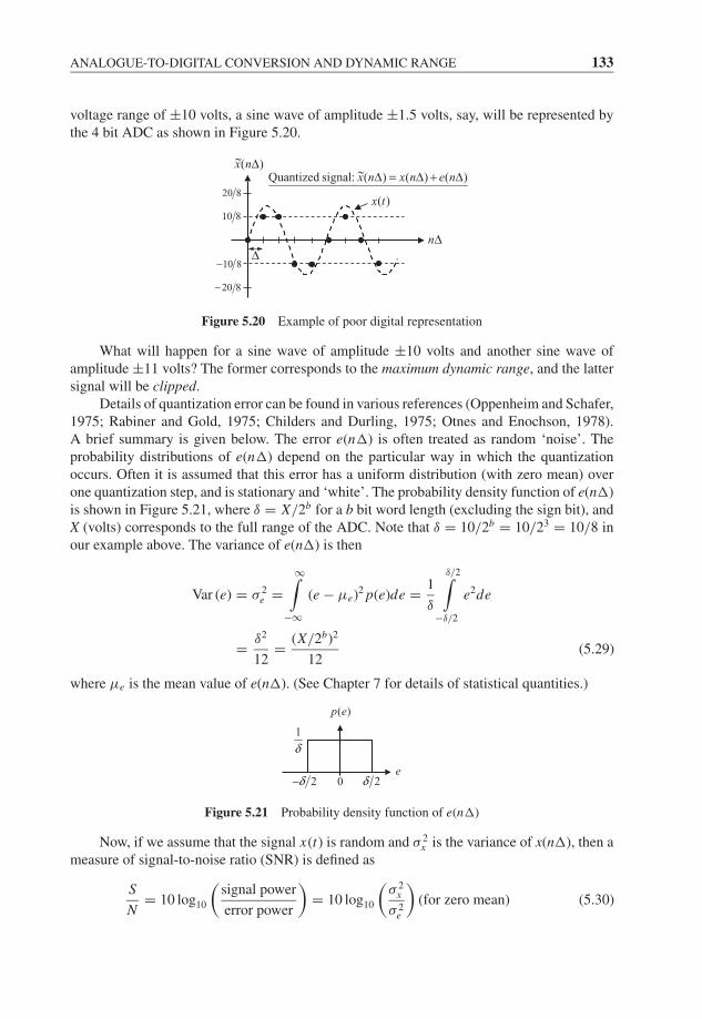
JWBK207-05 JWBK207-Shin January 26, 2008 17:5 Char Count= 0
ANALOGUE-TO-DIGITAL CONVERSION AND DYNAMIC RANGE 133
voltage range of ±10 volts, a sine wave of amplitude ±1.5 volts, say, will be represented bythe 4 bit ADC as shown in Figure 5.20.
Δ
( )x nΔ~~
20 8
Quantized signal: ( ) ( ) ( )x n x n e nΔ = Δ + Δ
( )x t10 8
10 8−
20 8−
nΔ
Figure 5.20 Example of poor digital representation
What will happen for a sine wave of amplitude ±10 volts and another sine wave ofamplitude ±11 volts? The former corresponds to the maximum dynamic range, and the lattersignal will be clipped.
Details of quantization error can be found in various references (Oppenheim and Schafer,1975; Rabiner and Gold, 1975; Childers and Durling, 1975; Otnes and Enochson, 1978).A brief summary is given below. The error e(n�) is often treated as random ‘noise’. Theprobability distributions of e(n�) depend on the particular way in which the quantizationoccurs. Often it is assumed that this error has a uniform distribution (with zero mean) overone quantization step, and is stationary and ‘white’. The probability density function of e(n�)is shown in Figure 5.21, where δ = X/2b for a b bit word length (excluding the sign bit), andX (volts) corresponds to the full range of the ADC. Note that δ = 10/2b = 10/23 = 10/8 inour example above. The variance of e(n�) is then
Var (e) = σ 2e =
∞∫−∞
(e − μe)2 p(e)de = 1
δ
δ/2∫−δ/2
e2de
= δ2
12= (X/2b)2
12(5.29)
where μe is the mean value of e(n�). (See Chapter 7 for details of statistical quantities.)
( )p e
1
δ
2δ− 2δ0e
Figure 5.21 Probability density function of e(n�)
Now, if we assume that the signal x(t) is random and σ 2x is the variance of x(n�), then a
measure of signal-to-noise ratio (SNR) is defined as
S
N= 10 log10
(signal power
error power
)= 10 log10
(σ 2
x
σ 2e
)(for zero mean) (5.30)
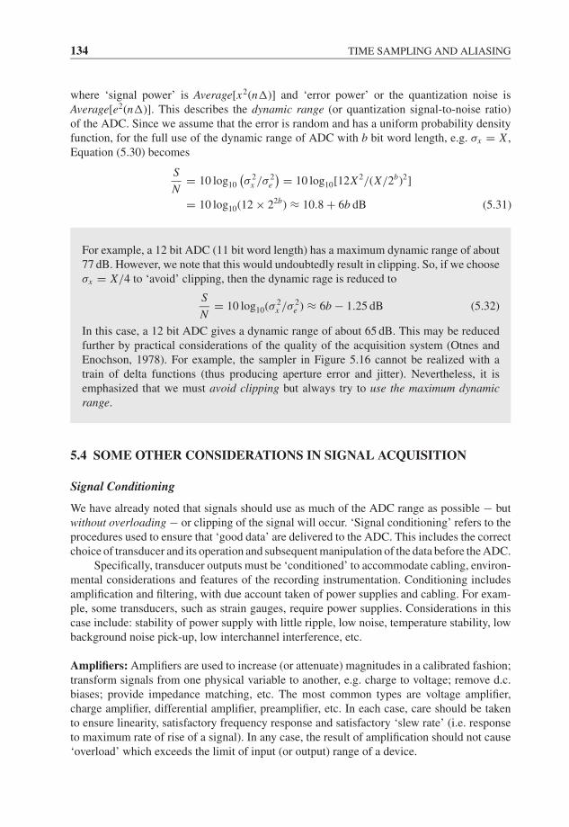
JWBK207-05 JWBK207-Shin January 26, 2008 17:5 Char Count= 0
134 TIME SAMPLING AND ALIASING
where ‘signal power’ is Average[x2(n�)] and ‘error power’ or the quantization noise isAverage[e2(n�)]. This describes the dynamic range (or quantization signal-to-noise ratio)of the ADC. Since we assume that the error is random and has a uniform probability densityfunction, for the full use of the dynamic range of ADC with b bit word length, e.g. σx = X ,Equation (5.30) becomes
S
N= 10 log10
(σ 2
x /σ 2e
) = 10 log10[12X2/(X/2b)2]
= 10 log10(12 × 22b) ≈ 10.8 + 6b dB (5.31)
For example, a 12 bit ADC (11 bit word length) has a maximum dynamic range of about77 dB. However, we note that this would undoubtedly result in clipping. So, if we chooseσx = X/4 to ‘avoid’ clipping, then the dynamic rage is reduced to
S
N= 10 log10(σ 2
x /σ 2e ) ≈ 6b − 1.25 dB (5.32)
In this case, a 12 bit ADC gives a dynamic range of about 65 dB. This may be reducedfurther by practical considerations of the quality of the acquisition system (Otnes andEnochson, 1978). For example, the sampler in Figure 5.16 cannot be realized with atrain of delta functions (thus producing aperture error and jitter). Nevertheless, it isemphasized that we must avoid clipping but always try to use the maximum dynamicrange.
5.4 SOME OTHER CONSIDERATIONS IN SIGNAL ACQUISITION
Signal Conditioning
We have already noted that signals should use as much of the ADC range as possible − butwithout overloading − or clipping of the signal will occur. ‘Signal conditioning’ refers to theprocedures used to ensure that ‘good data’ are delivered to the ADC. This includes the correctchoice of transducer and its operation and subsequent manipulation of the data before the ADC.
Specifically, transducer outputs must be ‘conditioned’ to accommodate cabling, environ-mental considerations and features of the recording instrumentation. Conditioning includesamplification and filtering, with due account taken of power supplies and cabling. For exam-ple, some transducers, such as strain gauges, require power supplies. Considerations in thiscase include: stability of power supply with little ripple, low noise, temperature stability, lowbackground noise pick-up, low interchannel interference, etc.
Amplifiers: Amplifiers are used to increase (or attenuate) magnitudes in a calibrated fashion;transform signals from one physical variable to another, e.g. charge to voltage; remove d.c.biases; provide impedance matching, etc. The most common types are voltage amplifier,charge amplifier, differential amplifier, preamplifier, etc. In each case, care should be takento ensure linearity, satisfactory frequency response and satisfactory ‘slew rate’ (i.e. responseto maximum rate of rise of a signal). In any case, the result of amplification should not cause‘overload’ which exceeds the limit of input (or output) range of a device.
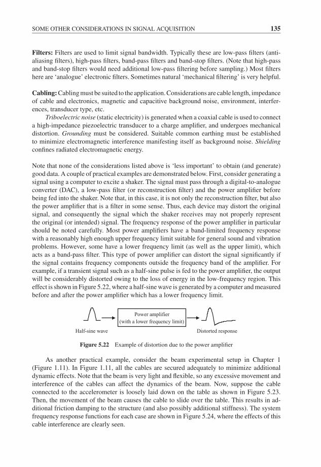
JWBK207-05 JWBK207-Shin January 26, 2008 17:5 Char Count= 0
SOME OTHER CONSIDERATIONS IN SIGNAL ACQUISITION 135
Filters: Filters are used to limit signal bandwidth. Typically these are low-pass filters (anti-aliasing filters), high-pass filters, band-pass filters and band-stop filters. (Note that high-passand band-stop filters would need additional low-pass filtering before sampling.) Most filtershere are ‘analogue’ electronic filters. Sometimes natural ‘mechanical filtering’ is very helpful.
Cabling: Cabling must be suited to the application. Considerations are cable length, impedanceof cable and electronics, magnetic and capacitive background noise, environment, interfer-ences, transducer type, etc.
Triboelectric noise (static electricity) is generated when a coaxial cable is used to connecta high-impedance piezoelectric transducer to a charge amplifier, and undergoes mechanicaldistortion. Grounding must be considered. Suitable common earthing must be establishedto minimize electromagnetic interference manifesting itself as background noise. Shieldingconfines radiated electromagnetic energy.
Note that none of the considerations listed above is ‘less important’ to obtain (and generate)good data. A couple of practical examples are demonstrated below. First, consider generating asignal using a computer to excite a shaker. The signal must pass through a digital-to-analogueconverter (DAC), a low-pass filter (or reconstruction filter) and the power amplifier beforebeing fed into the shaker. Note that, in this case, it is not only the reconstruction filter, but alsothe power amplifier that is a filter in some sense. Thus, each device may distort the originalsignal, and consequently the signal which the shaker receives may not properly representthe original (or intended) signal. The frequency response of the power amplifier in particularshould be noted carefully. Most power amplifiers have a band-limited frequency responsewith a reasonably high enough upper frequency limit suitable for general sound and vibrationproblems. However, some have a lower frequency limit (as well as the upper limit), whichacts as a band-pass filter. This type of power amplifier can distort the signal significantly ifthe signal contains frequency components outside the frequency band of the amplifier. Forexample, if a transient signal such as a half-sine pulse is fed to the power amplifier, the outputwill be considerably distorted owing to the loss of energy in the low-frequency region. Thiseffect is shown in Figure 5.22, where a half-sine wave is generated by a computer and measuredbefore and after the power amplifier which has a lower frequency limit.
Power amplifier
(with a lower frequency limit)
Distorted responseHalf-sine wave
Figure 5.22 Example of distortion due to the power amplifier
As another practical example, consider the beam experimental setup in Chapter 1(Figure 1.11). In Figure 1.11, all the cables are secured adequately to minimize additionaldynamic effects. Note that the beam is very light and flexible, so any excessive movement andinterference of the cables can affect the dynamics of the beam. Now, suppose the cableconnected to the accelerometer is loosely laid down on the table as shown in Figure 5.23.Then, the movement of the beam causes the cable to slide over the table. This results in ad-ditional friction damping to the structure (and also possibly additional stiffness). The systemfrequency response functions for each case are shown in Figure 5.24, where the effects of thiscable interference are clearly seen.

JWBK207-05 JWBK207-Shin January 26, 2008 17:5 Char Count= 0
136 TIME SAMPLING AND ALIASING
Cable interference
Figure 5.23 Experiment with cable interference
10 20 30 40 50 60 70 80 90–60
–50
–40
–30
–20
–10
0
10
20
30
40
Frequency (Hz)
Mag
nit
ud
e of
FR
F (
dB
)
Without cable interference
With cable interference
Figure 5.24 FRF of the system with/without cable interference
Data Validation
As demonstrated in the above experimental results, every possible effort should be madeearly in any experiment to ensure good data are captured. Data validation refers gener-ally to the many and varied checks and tests one may perform prior to ‘serious’ signalprocessing. This will occur at both analogue and digital stages. Obviously it would bebest always to process only ‘perfect’ signals. This ideal is impossible and a very clearunderstanding of any shortcomings in the data is vital.
A long list of items for consideration can be compiled, some of which are as follows:� Most signals will be recorded, even if some real-time processing is carried out. Identifyany physical events for correlation with data.� Inspect time histories critically, e.g. if periodic signals are expected, check for othersignals such as noise, transients.� Ensure non-stationary signals are adequately captured and note any changing ‘physics’that might account for the non-stationarity.
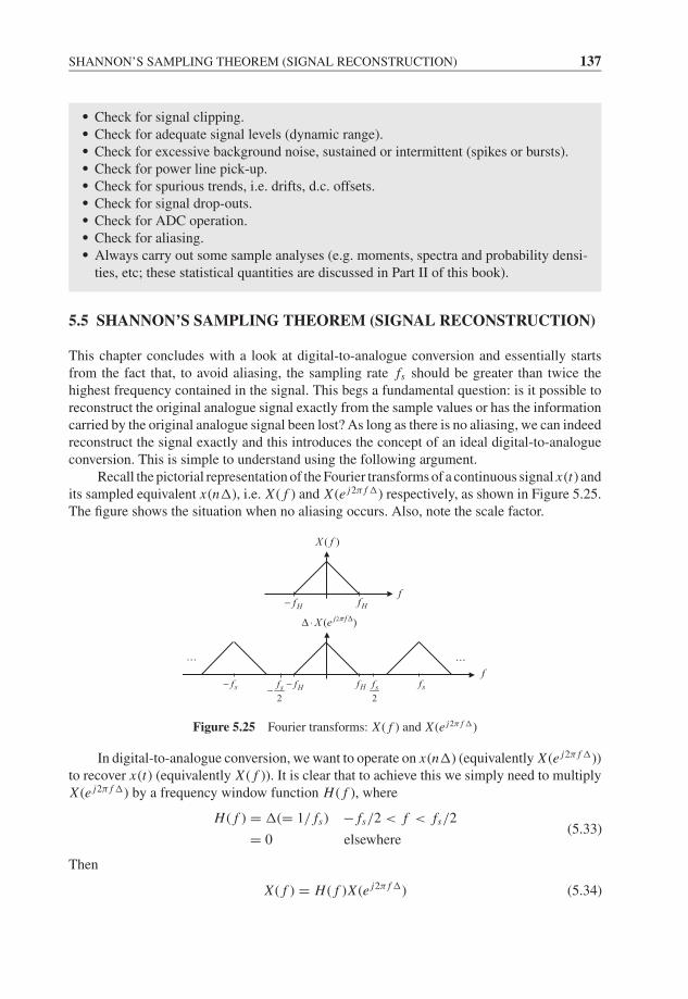
JWBK207-05 JWBK207-Shin January 26, 2008 17:5 Char Count= 0
SHANNON’S SAMPLING THEOREM (SIGNAL RECONSTRUCTION) 137
� Check for signal clipping.� Check for adequate signal levels (dynamic range).� Check for excessive background noise, sustained or intermittent (spikes or bursts).� Check for power line pick-up.� Check for spurious trends, i.e. drifts, d.c. offsets.� Check for signal drop-outs.� Check for ADC operation.� Check for aliasing.� Always carry out some sample analyses (e.g. moments, spectra and probability densi-ties, etc; these statistical quantities are discussed in Part II of this book).
5.5 SHANNON’S SAMPLING THEOREM (SIGNAL RECONSTRUCTION)
This chapter concludes with a look at digital-to-analogue conversion and essentially startsfrom the fact that, to avoid aliasing, the sampling rate fs should be greater than twice thehighest frequency contained in the signal. This begs a fundamental question: is it possible toreconstruct the original analogue signal exactly from the sample values or has the informationcarried by the original analogue signal been lost? As long as there is no aliasing, we can indeedreconstruct the signal exactly and this introduces the concept of an ideal digital-to-analogueconversion. This is simple to understand using the following argument.
Recall the pictorial representation of the Fourier transforms of a continuous signal x(t) andits sampled equivalent x(n�), i.e. X ( f ) and X (e j2π f �) respectively, as shown in Figure 5.25.The figure shows the situation when no aliasing occurs. Also, note the scale factor.
Hf
( )X f
Hf−f
Hf
2( )j fX e π ΔΔ ⋅
Hf−2sf sf
......f
2sf−sf−
Figure 5.25 Fourier transforms: X ( f ) and X (e j2π f �)
In digital-to-analogue conversion, we want to operate on x(n�) (equivalently X (e j2π f �))to recover x(t) (equivalently X ( f )). It is clear that to achieve this we simply need to multiplyX (e j2π f �) by a frequency window function H ( f ), where
H ( f ) = �(= 1/ fs) − fs/2 < f < fs/2
= 0 elsewhere(5.33)
Then
X ( f ) = H ( f )X (e j2π f �) (5.34)
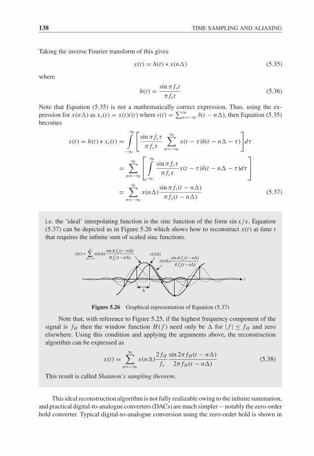
JWBK207-05 JWBK207-Shin January 26, 2008 17:5 Char Count= 0
138 TIME SAMPLING AND ALIASING
Taking the inverse Fourier transform of this gives
x(t) = h(t) ∗ x(n�) (5.35)
where
h(t) = sin π fs t
π fs t(5.36)
Note that Equation (5.35) is not a mathematically correct expression. Thus, using the ex-pression for x(n�) as xs(t) = x(t)i(t) where i(t) = ∑∞
n=−∞ δ(t − n�), then Equation (5.35)becomes
x(t) = h(t) ∗ xs(t) =∞∫
−∞
[sin π fsτ
π fsτ
∞∑n=−∞
x(t − τ )δ(t − n� − τ )
]dτ
=∞∑
n=−∞
⎡⎣ ∞∫−∞
sin π fsτ
π fsτx(t − τ )δ(t − n� − τ )dτ
⎤⎦=
∞∑n=−∞
x(n�)sin π fs(t − n�)
π fs(t − n�)(5.37)
i.e. the ‘ideal’ interpolating function is the sinc function of the form sin x/x . Equation(5.37) can be depicted as in Figure 5.26 which shows how to reconstruct x(t) at time tthat requires the infinite sum of scaled sinc functions.
( )x nΔsin ( )
( )( )s
s
f t nx n
f t n
ππ
− ΔΔ− Δ
t
sin ( )( ) ( )
( )s
n=−∞ s
f t nx t x n
f t n
ππ
∞ − Δ= Δ− Δ∑
Δ
Figure 5.26 Graphical representation of Equation (5.37)
Note that, with reference to Figure 5.25, if the highest frequency component of thesignal is fH then the window function H ( f ) need only be � for | f | ≤ fH and zeroelsewhere. Using this condition and applying the arguments above, the reconstructionalgorithm can be expressed as
x(t) =∞∑
n=−∞x(n�)
2 fH
fs
sin 2π fH (t − n�)
2π fH (t − n�)(5.38)
This result is called Shannon’s sampling theorem.
This ideal reconstruction algorithm is not fully realizable owing to the infinite summation,and practical digital-to-analogue converters (DACs) are much simpler − notably the zero-orderhold converter. Typical digital-to-analogue conversion using the zero-order hold is shown in
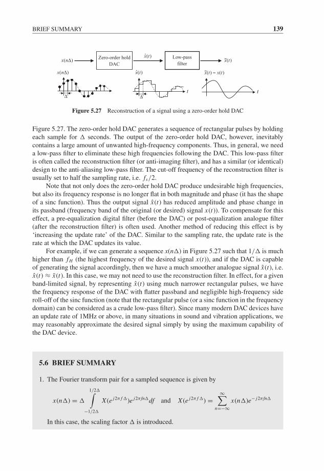
JWBK207-05 JWBK207-Shin January 26, 2008 17:5 Char Count= 0
BRIEF SUMMARY 139
Zero-order hold
DAC
Low-pass
filter( )x nΔ ( )x t~
ˆ( )x t
Δ
( )x nΔ
Δ
ˆ( )x t
t
( ) ( )x t x t≈~
t
Figure 5.27 Reconstruction of a signal using a zero-order hold DAC
Figure 5.27. The zero-order hold DAC generates a sequence of rectangular pulses by holdingeach sample for � seconds. The output of the zero-order hold DAC, however, inevitablycontains a large amount of unwanted high-frequency components. Thus, in general, we needa low-pass filter to eliminate these high frequencies following the DAC. This low-pass filteris often called the reconstruction filter (or anti-imaging filter), and has a similar (or identical)design to the anti-aliasing low-pass filter. The cut-off frequency of the reconstruction filter isusually set to half the sampling rate, i.e. fs/2.
Note that not only does the zero-order hold DAC produce undesirable high frequencies,but also its frequency response is no longer flat in both magnitude and phase (it has the shapeof a sinc function). Thus the output signal x(t) has reduced amplitude and phase change inits passband (frequency band of the original (or desired) signal x(t)). To compensate for thiseffect, a pre-equalization digital filter (before the DAC) or post-equalization analogue filter(after the reconstruction filter) is often used. Another method of reducing this effect is by‘increasing the update rate’ of the DAC. Similar to the sampling rate, the update rate is therate at which the DAC updates its value.
For example, if we can generate a sequence x(n�) in Figure 5.27 such that 1/� is muchhigher than fH (the highest frequency of the desired signal x(t)), and if the DAC is capableof generating the signal accordingly, then we have a much smoother analogue signal x(t), i.e.x(t) ≈ x(t). In this case, we may not need to use the reconstruction filter. In effect, for a givenband-limited signal, by representing x(t) using much narrower rectangular pulses, we havethe frequency response of the DAC with flatter passband and negligible high-frequency sideroll-off of the sinc function (note that the rectangular pulse (or a sinc function in the frequencydomain) can be considered as a crude low-pass filter). Since many modern DAC devices havean update rate of 1MHz or above, in many situations in sound and vibration applications, wemay reasonably approximate the desired signal simply by using the maximum capability ofthe DAC device.
5.6 BRIEF SUMMARY
1. The Fourier transform pair for a sampled sequence is given by
x(n�) = �
1/2�∫−1/2�
X (e j2π f �)e j2π fn�df and X (e j2π f �) =∞∑
n=−∞x(n�)e− j2π fn�
In this case, the scaling factor � is introduced.

JWBK207-05 JWBK207-Shin January 26, 2008 17:5 Char Count= 0
140 TIME SAMPLING AND ALIASING
2. The relationship between the Fourier transform of a continuous signal and the Fouriertransform of the corresponding sampled sequence is
X (e j2π f �) = 1
�
∞∑n=−∞
X(
f − n
�
)i.e. X (e j2π f �) is a continuous function consisting of replicas of scaled X ( f ), and isperiodic with period 1/�. This introduces possible aliasing.
3. To avoid aliasing, an ‘analogue’ low-pass filter (anti-aliasing filter) must be used beforethe analogue-to-digital conversion, and the sampling rate of the ADC must be highenough. In practice, for a given anti-aliasing filter with a roll-off rate of B dB/octaveand an ADC with a dynamic range of A dB, the sampling rate is chosen as
fs ≈ 2 × 100.3A/B fc
4. To obtain ‘good’ data, we need to use the maximum dynamic range of the ADC (butmust avoid clipping). Also, care must be taken with any signal conditioning, filters,amplifiers, cabling, etc.
5. When generating an analogue signal, for some applications, we may not need areconstruction filter if the update rate of the DAC is high.
5.7 MATLAB EXAMPLES
Example 5.1: Demonstration of aliasing
Case A: This example demonstrates that the values ±p + k/� Hz become aliases offrequency p Hz. (see Figure 5.11).
Consider that we want to sample a sinusoidal signal x(t) = sin 2πpt with the sam-pling rate fs = 100 Hz. We examine three cases: x1(t) = sin 2πp1t , x2(t) = sin 2πp2tand x3(t) = sin 2πp3t where p1 = 20 Hz, p2 = 80 Hz and p3 = 120 Hz. Note that allthe frequencies will appear at the same frequency of 20 Hz.
Line MATLAB code Comments
1 clear all Define the sampling rate fs = 100 Hz, total recordtime T = 10 seconds, and the time variable t from 0to ‘T-1/fs’ seconds. Also define the frequencies foreach sinusoid.
2 fs=100; T=10;3 t=0:1/fs:T-1/fs;4 p1=20; p2=80; p3=120;
5 x1=sin(2*pi*p1*t); Generate the signals x1(t), x2(t) and x3(t). Note thatall these signals use the same time variable ‘t’, thus ithas the same sampling rate.
6 x2=sin(2*pi*p2*t);7 x3=sin(2*pi*p3*t);
8 N=length(t); Perform the DFT of each signal, and calculate thefrequency variable f.

JWBK207-05 JWBK207-Shin January 26, 2008 17:5 Char Count= 0
MATLAB EXAMPLES 141
9 X1=fft(x1); X2=fft(x2);X3=fft(x3);
10 f=fs*(0:N-1)/N;
11 figure(1); plot(f, abs(X1)/fs/T) Plot the modulus of the DFT of x1(t) = sin 2π (20)tfor the frequency range 0 Hz to 100 Hz (i.e. up to thesampling frequency). Note that the right half of thegraph is the mirror image of the left half (except the0 Hz component).
12 xlabel('Frequency (Hz)');ylabel('Modulus')
13 axis([0 100 0 0.55])
14 figure(2); plot(f, abs(X2)/fs/T) Plot the modulus of the DFT of x2(t) = sin 2π (80)t .15 xlabel('Frequency (Hz)');
ylabel('Modulus')16 axis([0 100 0 0.55])
17 figure(3); plot(f, abs(X3)/fs/T) Plot the modulus of the DFT of x3(t) = sin 2π (120)t .18 xlabel('Frequency (Hz)');
ylabel('Modulus')19 axis([0 100 0 0.55])
Results
0 10 20 30 40 50 60 70 80 90 1000
0.1
0.2
0.3
0.4
0.5
Frequency (Hz)
Modulu
s
1 20 Hz,p =
2 380 Hz, 120 Hzp p= =and aliases of
2sf sf
Comments: Note that all the frequencies p1 = 20 Hz, p2 = 80 Hz and p3 = 120 Hzappear at the same frequency 20 Hz.
Example 5.2: Demonstration of aliasing
Case B: This example demonstrates the aliasing problem on the ‘digital’ sampling of asampled sequence x(n�).
Consider a sampled sinusoidal sequence x(n�) = sin 2πpn� where p = 40 Hz,and the sampling rate is fs = 500 Hz ( fs = 1/�). Now, sample this sequence digitallyagain, i.e. generate a new sequence x1(k�) = x[(5k)�], k = 0, 1, 2, . . . , by taking everyfive sample values of x(n�) (this has the effect of reducing the sampling rate to 100 Hz).Also generate a sequence x2(k�) = x[(10k)�] by taking every 10 sample values ofx(n�), which reduces the sampling rate to 50 Hz. Thus, aliasing occurs, i.e. p = 40 Hzwill appear at 10 Hz.
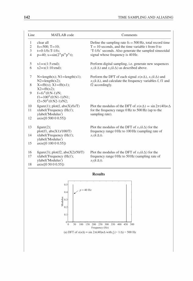
JWBK207-05 JWBK207-Shin January 26, 2008 17:5 Char Count= 0
142 TIME SAMPLING AND ALIASING
Line MATLAB code Comments
1 clear all Define the sampling rate fs = 500 Hz, total record timeT = 10 seconds, and the time variable t from 0 to‘T-1/fs’ seconds. Also generate the sampled sinusoidalsignal whose frequency is 40 Hz.
2 fs=500; T=10;3 t=0:1/fs:T-1/fs;4 p=40; x=sin(2*pi*p*t);
5 x1=x(1:5:end); Perform digital sampling, i.e. generate new sequencesx1(k�) and x2(k�) as described above.6 x2=x(1:10:end);
7 N=length(x); N1=length(x1);N2=length(x2);
Perform the DFT of each signal x(n�), x1(k�) andx2(k�), and calculate the frequency variables f, f1 andf2 accordingly.8 X=fft(x); X1=fft(x1);
X2=fft(x2);9 f=fs*(0:N-1)/N;
f1=100*(0:N1-1)/N1;f2=50*(0:N2-1)/N2;
10 figure(1); plot(f, abs(X)/fs/T) Plot the modulus of the DFT of x(n�) = sin 2π (40)n�for the frequency range 0 Hz to 500 Hz (up to thesampling rate).
11 xlabel('Frequency (Hz)');ylabel('Modulus')
12 axis([0 500 0 0.55])
13 figure(2);plot(f1, abs(X1)/100/T)
Plot the modulus of the DFT of x1(k�) for thefrequency range 0 Hz to 100 Hz (sampling rate ofx1(k�)).14 xlabel('Frequency (Hz)');
ylabel('Modulus')15 axis([0 100 0 0.55])
16 figure(3); plot(f2, abs(X2)/50/T) Plot the modulus of the DFT of x2(k�) for thefrequency range 0 Hz to 50 Hz (sampling rate ofx2(k�)).
17 xlabel('Frequency (Hz)');ylabel('Modulus')
18 axis([0 50 0 0.55])
Results
0 50 100 150 200 250 300 350 400 450 5000
0.1
0.2
0.3
0.4
0.5
Frequency (Hz)
Mo
du
lus
40 Hzp =
(a) DFT of x(nΔ) = sin 2π(40)nΔ with f (= 1/Δ) = 500 Hzs

JWBK207-05 JWBK207-Shin January 26, 2008 17:5 Char Count= 0
MATLAB EXAMPLES 143
0 10 20 30 40 50 60 70 80 90 1000
0.1
0.2
0.3
0.4
0.5
Frequency (Hz)
Mo
du
lus
40 Hzp =
0 5 10 15 20 25 30 35 40 45 500
0.1
0.2
0.3
0.4
0.5
Frequency (Hz)
Mo
du
lus
Alias of p = 40 Hz
(b) DFT of x1 (kΔ) = x[(5k)Δ] (c) DFT of x2 (kΔ) = x[(10k)Δ]
Comments: Note that aliasing occurs in the third case, i.e. p = 40 Hz appears at 10 Hzbecause the sampling rate is 50 Hz in this case.
Example 5.3: Demonstration of ‘digital’ anti-aliasing filtering
This example demonstrates a method to overcome the problem addressed in the previousMATLAB example.
We use the MATLAB function ‘resample’ to avoid the aliasing problem. The‘resample’ function applies the digital anti-aliasing filter to the sequence before thesampling.
Consider a sampled sinusoidal sequence x(n�) = sin 2πp1n� + sin 2πp2n�
where p1 = 10 Hz and p2 = 40 Hz and the sampling rate is fs = 500 Hz ( fs = 1/�).Generate new sequences x1(k�1) and x2(k�2) from x(n�) such that �1/� = 5 and�2/� = 10 without causing aliasing using the ‘resample’ function.
Line MATLAB code Comments
1 clear all Define the sampling rate fs = 500 Hz, totalrecord time T = 10 seconds, and the timevariable t from 0 to ‘T-1/fs’ seconds. Alsogenerate the sampled signal whose frequencycomponents are 10 Hz and 40 Hz.
2 fs=500; T=10;3 t=0:1/fs:T-1/fs; p1=10; p2=40;4 x=sin(2*pi*p1*t) + sin(2*pi*p2*t);
5 x1=resample(x,100,500); Perform the ‘resampling’ as described above.6 x2=resample(x,50,500); For example, the function ‘resample(x,100,500)’
takes the sequence ‘x’, applies a low-pass filterappropriately to the sequence, and returns theresampled sequence, where ‘100’ is the newsampling rate and ‘500’ is the original samplingrate.
7 N=length(x); N1=length(x1);N2=length(x2);
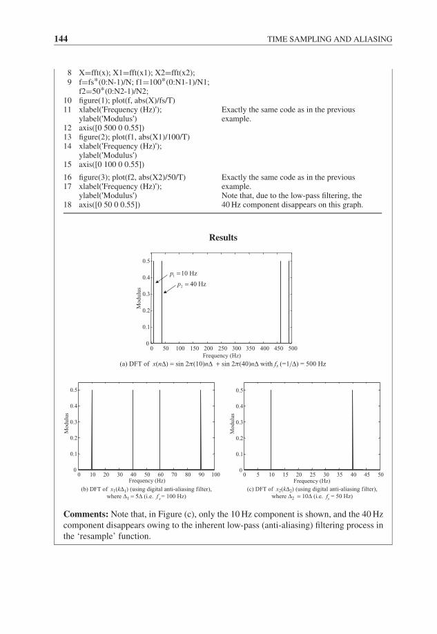
JWBK207-05 JWBK207-Shin January 26, 2008 17:5 Char Count= 0
144 TIME SAMPLING AND ALIASING
8 X=fft(x); X1=fft(x1); X2=fft(x2);9 f=fs*(0:N-1)/N; f1=100*(0:N1-1)/N1;
f2=50*(0:N2-1)/N2;10 figure(1); plot(f, abs(X)/fs/T)11 xlabel('Frequency (Hz)');
ylabel('Modulus')Exactly the same code as in the previousexample.
12 axis([0 500 0 0.55])13 figure(2); plot(f1, abs(X1)/100/T)14 xlabel('Frequency (Hz)');
ylabel('Modulus')15 axis([0 100 0 0.55])
16 figure(3); plot(f2, abs(X2)/50/T) Exactly the same code as in the previousexample.Note that, due to the low-pass filtering, the40 Hz component disappears on this graph.
17 xlabel('Frequency (Hz)');ylabel('Modulus')
18 axis([0 50 0 0.55])
Results
1 10 Hzp =
0 50 100 150 200 250 300 350 400 450 5000
0.1
0.2
0.3
0.4
0.5
Frequency (Hz)
Mo
du
lus 2 40 Hzp =
(a) DFT of x(nΔ) = sin 2π(10)nΔ + sin 2π(40)nΔ with f (=1/Δ) = 500 Hzs
0 10 20 30 40 50 60 70 80 90 1000
0.1
0.2
0.3
0.4
0.5
Frequency (Hz)
Mo
du
lus
0 5 10 15 20 25 30 35 40 45 500
0.1
0.2
0.3
0.4
0.5
Frequency (Hz)
Mo
du
lus
(b) DFT of x1(kΔ1) (using digital anti-aliasing filter),
where Δ1 = 5Δ (i.e. f = 100 Hz)s
(c) DFT of x2(kΔ2) (using digital anti-aliasing filter),
where Δ2 = 10Δ (i.e. f = 50 Hz)s
Comments: Note that, in Figure (c), only the 10 Hz component is shown, and the 40 Hzcomponent disappears owing to the inherent low-pass (anti-aliasing) filtering process inthe ‘resample’ function.
JWBK207-06 JWBK207-Shin January 26, 2008 18:29 Char Count= 0
6The Discrete Fourier Transform
Introduction
In this chapter we develop the properties of a fundamental tool of digital signal analysis −the discrete Fourier transform (DFT). This will include aspects of linear filtering, andrelating the DFT to other Fourier representations. The chapter concludes with an intro-duction to the fast Fourier transform (FFT).
6.1 SEQUENCES AND LINEAR FILTERS
Sequences
A sequence (or digital signal) is a function which is defined at a discrete set of points.A sequence results from: (i) a process which is naturally discrete such as a daily postedcurrency exchange rate, and (ii) sampling (at � second intervals (say)) an analogue signalas in Chapter 5. We shall denote a sequences as x(n). This is an ordered set of numbersas shown in Figure 6.1.
( )x n
−2 −1 0 1 2 3 4 5n
Figure 6.1 Example of a sequence
Some examples are listed below:
Fundamentals of Signal Processing for Sound and Vibration EngineersK. Shin and J. K. Hammond. C© 2008 John Wiley & Sons, Ltd
145
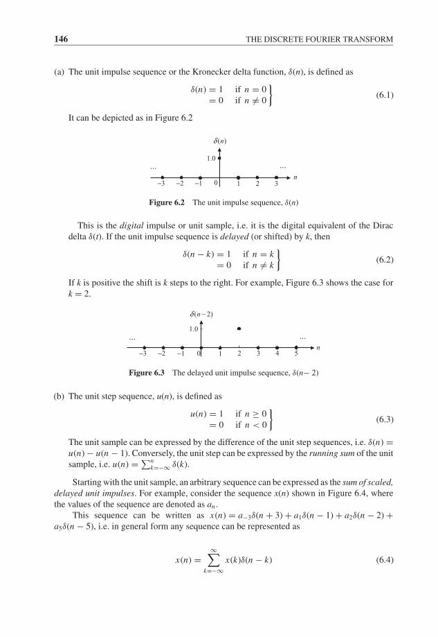
JWBK207-06 JWBK207-Shin January 26, 2008 18:29 Char Count= 0
146 THE DISCRETE FOURIER TRANSFORM
(a) The unit impulse sequence or the Kronecker delta function, δ(n), is defined as
δ(n) = 1 if n = 0= 0 if n �= 0
}(6.1)
It can be depicted as in Figure 6.2
......
−2 −1 0
1.0
1 2−3 3
( )nδ
n
Figure 6.2 The unit impulse sequence, δ(n)
This is the digital impulse or unit sample, i.e. it is the digital equivalent of the Diracdelta δ(t). If the unit impulse sequence is delayed (or shifted) by k, then
δ(n − k) = 1 if n = k= 0 if n �= k
}(6.2)
If k is positive the shift is k steps to the right. For example, Figure 6.3 shows the case fork = 2.
......
−2 −1 0
1.0
1 2 543−3
( 2)nδ −
n
Figure 6.3 The delayed unit impulse sequence, δ(n− 2)
(b) The unit step sequence, u(n), is defined as
u(n) = 1 if n ≥ 0= 0 if n < 0
}(6.3)
The unit sample can be expressed by the difference of the unit step sequences, i.e. δ(n) =u(n) − u(n − 1). Conversely, the unit step can be expressed by the running sum of the unitsample, i.e. u(n) = ∑n
k=−∞ δ(k).
Starting with the unit sample, an arbitrary sequence can be expressed as the sum of scaled,delayed unit impulses. For example, consider the sequence x(n) shown in Figure 6.4, wherethe values of the sequence are denoted as an .
This sequence can be written as x(n) = a−3δ(n + 3) + a1δ(n − 1) + a2δ(n − 2) +a5δ(n − 5), i.e. in general form any sequence can be represented as
x(n) =∞∑
k=−∞x(k)δ(n − k) (6.4)

JWBK207-06 JWBK207-Shin January 26, 2008 18:29 Char Count= 0
SEQUENCES AND LINEAR FILTERS 147
−2 −1 0 1 2 3 4 5−3−4
( )x n
n
3a− 2a
1a 5a
Figure 6.4 An arbitrary sequence, x(n)
Linear Filters
Discrete Linear Time (Shift) Invariant SystemsM6.1
The input–output relationship for a discrete LTI system (a digital filter) is shown inFigure 6.5.
y(n)x(n)Discrete LTI system
h(n)Output sequenceInput sequence
Figure 6.5 A discrete LTI system
Similar to the continuous LTI system, we define the impulse response sequence ofthe discrete LTI system as h(n). If the input to the system is a scaled and delayed impulseat k, i.e. x(n) = akδ(n − k), then the response of the system at n is y(n) = akh(n − k).So, for a general input sequence, the response at n due to input x(k) is h(n − k)x(k). Sinceany input can be expressed as the sum of scaled, delayed unit impulses as described inEquation (6.4), the total response y(n) to the input sequence x(n) is
y(n) =n∑
k=−∞h(n − k)x(k) if the system is causal (6.5a)
or
y(n) =∞∑
k=−∞h(n − k)x(k) if the system is non-causal (6.5b)
We shall use the latter notation (6.5b) which includes the former (6.5a) as a specialcase when h(n) = 0, if n < 0. This expression is called the convolution sum, whichdescribes the relationship between the input and the output. That is, the input–outputrelationship of the digital LTI system is expressed by the convolution of two sequencesx(n) and h(n):
y(n) = x(n) ∗ h(n) =∞∑
k=−∞h(n − k)x(k) (6.6)
Note that the convolution sum satisfies the property of commutativity, i.e.
y(n) =∞∑
k=−∞h(n − k)x(k) =
∞∑r=−∞
h(r )x(n − r ) (6.7a)
or simply
y(n) = x(n) ∗ h(n) = h(n) ∗ x(n) (6.7b)

JWBK207-06 JWBK207-Shin January 26, 2008 18:29 Char Count= 0
148 THE DISCRETE FOURIER TRANSFORM
The above expressions for the convolution sum are analogous to the convolution integralfor a continuous system (see Equations (4.51), (4.53)). An example of the convolution sumis demonstrated graphically in Figure 6.6. In this figure, note that the number of non-zeroelements of sequence y(n) is ‘12’ which is one element shorter than the sum of the lengths ofnon-zero elements of sequences x(n) and h(n).
h n( )x n
(2) (2 ) ( )∞
∑
∞∑
( )
n70
n0 4
y h k x k= −k=−∞
0
( ) ( ) ( ) ( ) ( ) (not to scale)= ∗ = −k=−∞
y n x n h n h n k x k
n0 11
Figure 6.6 Illustrations of a convolution sum M6.1
Relationship to Continuous Systems
Starting from y(t) = h(t) ∗ x(t) = ∫ ∞−∞ h(τ )x(t − τ )dτ , consider that the signals are sam-
pled such that y(n�) = h(n�) ∗ x(n�). Then the approximation to the convolution integralbecomes
y(n�) ≈∞∑
r=−∞h(r�)x((n − r )�) · � (6.8)
Note the scaling factor �, i.e. if the discrete LTI system h(n) results from the sampling of thecorresponding continuous system h(t) with sampling rate 1/� and the input x(n) is also thesampled version of x(t), then it follows that
y(n�) ≈ y(n) · � (6.9)
where y(n) = h(n) ∗ x(n).The concept of creating a digital filter h(n) by simply sampling the impulse response of
an analogue filter h(t) is called ‘impulse-invariant’ filter design (see Figure 5.6 in Section 5.1).
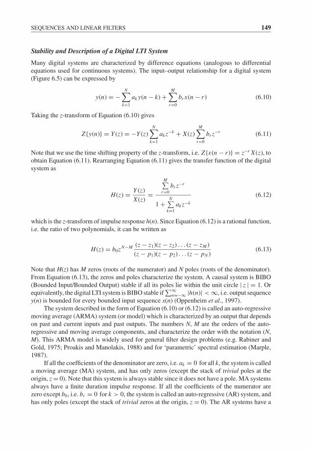
JWBK207-06 JWBK207-Shin January 26, 2008 18:29 Char Count= 0
SEQUENCES AND LINEAR FILTERS 149
Stability and Description of a Digital LTI System
Many digital systems are characterized by difference equations (analogous to differentialequations used for continuous systems). The input–output relationship for a digital system(Figure 6.5) can be expressed by
y(n) = −N∑
k=1
ak y(n − k) +M∑
r=0
br x(n − r ) (6.10)
Taking the z-transform of Equation (6.10) gives
Z{y(n)} = Y (z) = −Y (z)N∑
k=1
ak z−k + X (z)M∑
r=0
br z−r (6.11)
Note that we use the time shifting property of the z-transform, i.e. Z{x(n − r )} = z−r X (z), toobtain Equation (6.11). Rearranging Equation (6.11) gives the transfer function of the digitalsystem as
H (z) = Y (z)
X (z)=
M∑r=0
br z−r
1 +N∑
k=1
ak z−k
(6.12)
which is the z-transform of impulse response h(n). Since Equation (6.12) is a rational function,i.e. the ratio of two polynomials, it can be written as
H (z) = b0zN−M (z − z1)(z − z2) . . . (z − zM )
(z − p1)(z − p2) . . . (z − pN )(6.13)
Note that H(z) has M zeros (roots of the numerator) and N poles (roots of the denominator).From Equation (6.13), the zeros and poles characterize the system. A causal system is BIBO(Bounded Input/Bounded Output) stable if all its poles lie within the unit circle | z | = 1. Orequivalently, the digital LTI system is BIBO stable if
∑∞n=−∞ |h(n)| < ∞, i.e. output sequence
y(n) is bounded for every bounded input sequence x(n) (Oppenheim et al., 1997).The system described in the form of Equation (6.10) or (6.12) is called an auto-regressive
moving average (ARMA) system (or model) which is characterized by an output that dependson past and current inputs and past outputs. The numbers N, M are the orders of the auto-regressive and moving average components, and characterize the order with the notation (N,M). This ARMA model is widely used for general filter design problems (e.g. Rabiner andGold, 1975; Proakis and Manolakis, 1988) and for ‘parametric’ spectral estimation (Marple,1987).
If all the coefficients of the denominator are zero, i.e. ak = 0 for all k, the system is calleda moving average (MA) system, and has only zeros (except the stack of trivial poles at theorigin, z = 0). Note that this system is always stable since it does not have a pole. MA systemsalways have a finite duration impulse response. If all the coefficients of the numerator arezero except b0, i.e. br = 0 for k > 0, the system is called an auto-regressive (AR) system, andhas only poles (except the stack of trivial zeros at the origin, z = 0). The AR systems have a
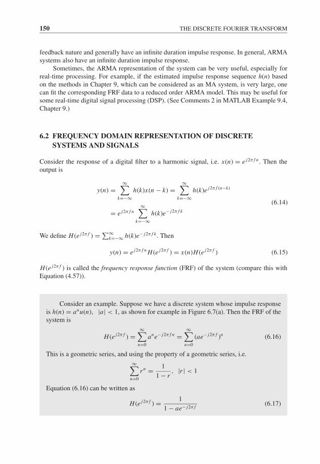
JWBK207-06 JWBK207-Shin January 26, 2008 18:29 Char Count= 0
150 THE DISCRETE FOURIER TRANSFORM
feedback nature and generally have an infinite duration impulse response. In general, ARMAsystems also have an infinite duration impulse response.
Sometimes, the ARMA representation of the system can be very useful, especially forreal-time processing. For example, if the estimated impulse response sequence h(n) basedon the methods in Chapter 9, which can be considered as an MA system, is very large, onecan fit the corresponding FRF data to a reduced order ARMA model. This may be useful forsome real-time digital signal processing (DSP). (See Comments 2 in MATLAB Example 9.4,Chapter 9.)
6.2 FREQUENCY DOMAIN REPRESENTATION OF DISCRETESYSTEMS AND SIGNALS
Consider the response of a digital filter to a harmonic signal, i.e. x(n) = e j2π f n . Then theoutput is
y(n) =∞∑
k=−∞h(k)x(n − k) =
∞∑k=−∞
h(k)e j2π f (n−k)
= e j2π f n∞∑
k=−∞h(k)e− j2π f k
(6.14)
We define H (e j2π f ) = ∑∞k=−∞ h(k)e− j2π f k . Then
y(n) = e j2π f n H (e j2π f ) = x(n)H (e j2π f ) (6.15)
H (e j2π f ) is called the frequency response function (FRF) of the system (compare this withEquation (4.57)).
Consider an example. Suppose we have a discrete system whose impulse responseis h(n) = anu(n), |a| < 1, as shown for example in Figure 6.7(a). Then the FRF of thesystem is
H (e j2π f ) =∞∑
n=0
ane− j2π f n =∞∑
n=0
(ae− j2π f )n (6.16)
This is a geometric series, and using the property of a geometric series, i.e.
∞∑n=0
rn = 1
1 − r, |r | < 1
Equation (6.16) can be written as
H (e j2π f ) = 1
1 − ae− j2π f(6.17)
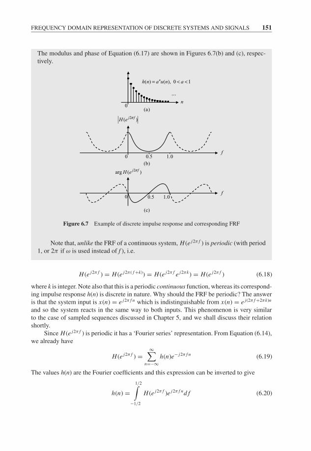
JWBK207-06 JWBK207-Shin January 26, 2008 18:29 Char Count= 0
FREQUENCY DOMAIN REPRESENTATION OF DISCRETE SYSTEMS AND SIGNALS 151
The modulus and phase of Equation (6.17) are shown in Figures 6.7(b) and (c), respec-tively.
( ) ( ), 0 1nh n a u n a= < <
...
0n
(a)
0
2( )j fH e π
0.5 1.0
(b)
f
2arg ( )j fH e π
0 0.5 1.0
(c)
f
Figure 6.7 Example of discrete impulse response and corresponding FRF
Note that, unlike the FRF of a continuous system, H (e j2π f ) is periodic (with period1, or 2π if ω is used instead of f ), i.e.
H (e j2π f ) = H (e j2π ( f +k)) = H (e j2π f e j2πk) = H (e j2π f ) (6.18)
where k is integer. Note also that this is a periodic continuous function, whereas its correspond-ing impulse response h(n) is discrete in nature. Why should the FRF be periodic? The answeris that the system input is x(n) = e j2π f n which is indistinguishable from x(n) = e j(2π f +2πk)n
and so the system reacts in the same way to both inputs. This phenomenon is very similarto the case of sampled sequences discussed in Chapter 5, and we shall discuss their relationshortly.
Since H (e j2π f ) is periodic it has a ‘Fourier series’ representation. From Equation (6.14),we already have
H (e j2π f ) =∞∑
n=−∞h(n)e− j2π f n (6.19)
The values h(n) are the Fourier coefficients and this expression can be inverted to give
h(n) =1/2∫
−1/2
H (e j2π f )e j2π f nd f (6.20)

JWBK207-06 JWBK207-Shin January 26, 2008 18:29 Char Count= 0
152 THE DISCRETE FOURIER TRANSFORM
Equation (6.20) is easily justified by considering the Fourier series pair given in Chapter 3,i.e.
x(t) =∞∑
n=−∞cne j2πnt/TP
and
cn = 1
TP
TP∫0
x(t)e− j2πnt/TP dt
The two expressions (6.19) and (6.20) are the basis of the Fourier representation ofdiscrete signals and apply to any sequence provided that Equation (6.19) converges. Equation(6.19) is the Fourier transform of a sequence, and is often called the discrete-time Fouriertransform (Oppenheim et al., 1997). However, this should not be confused with discreteFourier transform (DFT) for finite length signals that will be discussed in the next section.Alternatives to Equations (6.19) and (6.20) are
H (e jω) =∞∑
n=−∞h(n)e− jωn (6.21)
h(n) = 1
2π
π∫−π
H (e jω)e jωndω (6.22)
Note that, similar to the Fourier integral, if h(n) is real,∣∣H (e j2π f )
∣∣ is an even and arg H (e j2π f )is an odd function of ‘f ’.
The Fourier Transform of the Convolution of Two Sequences
Let us consider an output sequence of a discrete LTI system, which is the convolution of twosequences h(n) and x(n), i.e. y(n) = h(n) ∗ x(n) = ∑∞
k=−∞ h(k)x(n − k). Since the sequence
x(n) has a Fourier representation, i.e. x(n) = ∫ 1/2
−1/2X (e j2π f )e j2π f nd f , substituting this into
the convolution expression gives
y(n) =∞∑
k=−∞h(k)x(n − k) =
∞∑k=−∞
h(k)
1/2∫−1/2
X (e j2π f )e j2π f (n−k)d f
=1/2∫
−1/2
X (e j2π f )∞∑
k=−∞h(k)e− j2π f k
︸ ︷︷ ︸H (e j2π f )
e j2π f nd f =1/2∫
−1/2
X (e j2π f )H (e j2π f )e j2π f nd f
(6.23)Thus,
Y (e j2π f ) = X (e j2π f )H (e j2π f ) (6.24)
i.e. the Fourier transform of the convolution of two sequences is the product of their transforms.
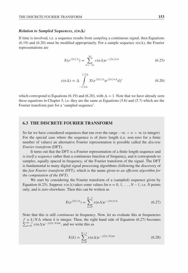
JWBK207-06 JWBK207-Shin January 26, 2008 18:29 Char Count= 0
THE DISCRETE FOURIER TRANSFORM 153
Relation to Sampled Sequences, x(nΔ)
If time is involved, i.e. a sequence results from sampling a continuous signal, then Equations(6.19) and (6.20) must be modified appropriately. For a sample sequence x(n�), the Fourierrepresentations are
X (e j2π f �) =∞∑
n=−∞x(n�)e− j2π f n� (6.25)
x(n�) = �
1/2�∫−1/2�
X (e j2π f �)e j2π f n�d f (6.26)
which correspond to Equations (6.19) and (6.20), with � = 1. Note that we have already seenthese equations in Chapter 5, i.e. they are the same as Equations (5.6) and (5.7) which are theFourier transform pair for a ‘sampled sequence’.
6.3 THE DISCRETE FOURIER TRANSFORM
So far we have considered sequences that run over the range −∞ < n < ∞ (n integer).For the special case where the sequence is of finite length (i.e. non-zero for a finitenumber of values) an alternative Fourier representation is possible called the discreteFourier transform (DFT).
It turns out that the DFT is a Fourier representation of a finite length sequence andis itself a sequence rather than a continuous function of frequency, and it corresponds tosamples, equally spaced in frequency, of the Fourier transform of the signal. The DFTis fundamental to many digital signal processing algorithms (following the discovery ofthe fast Fourier transform (FFT), which is the name given to an efficient algorithm forthe computation of the DFT).
We start by considering the Fourier transform of a (sampled) sequence given byEquation (6.25). Suppose x(n�) takes some values for n = 0, 1, . . . , N − 1, i.e. N pointsonly, and is zero elsewhere. Then this can be written as
X (e j2π f �) =N−1∑n=0
x(n�)e− j2π f n� (6.27)
Note that this is still continuous in frequency. Now, let us evaluate this at frequenciesf = k/N� where k is integer. Then, the right hand side of Equation (6.27) becomes∑N−1
n=0 x(n�)e− j(2π/N )nk , and we write this as
X (k) =N−1∑n=0
x(n�)e− j(2π/N )nk (6.28)
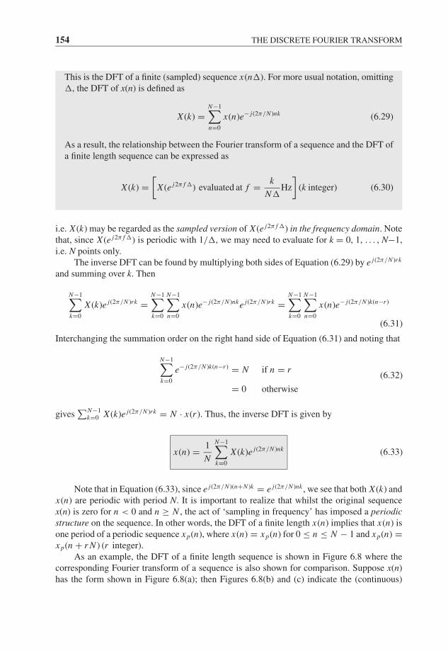
JWBK207-06 JWBK207-Shin January 26, 2008 18:29 Char Count= 0
154 THE DISCRETE FOURIER TRANSFORM
This is the DFT of a finite (sampled) sequence x(n�). For more usual notation, omitting�, the DFT of x(n) is defined as
X (k) =N−1∑n=0
x(n)e− j(2π/N )nk (6.29)
As a result, the relationship between the Fourier transform of a sequence and the DFT ofa finite length sequence can be expressed as
X (k) =[
X (e j2π f �) evaluated at f = k
N�Hz
](k integer) (6.30)
i.e. X (k) may be regarded as the sampled version of X (e j2π f �) in the frequency domain. Notethat, since X (e j2π f �) is periodic with 1/�, we may need to evaluate for k = 0, 1, . . . , N−1,i.e. N points only.
The inverse DFT can be found by multiplying both sides of Equation (6.29) by e j(2π/N )rk
and summing over k. Then
N−1∑k=0
X (k)e j(2π/N )rk =N−1∑k=0
N−1∑n=0
x(n)e− j(2π/N )nke j(2π/N )rk =N−1∑k=0
N−1∑n=0
x(n)e− j(2π/N )k(n−r )
(6.31)
Interchanging the summation order on the right hand side of Equation (6.31) and noting that
N−1∑k=0
e− j(2π/N )k(n−r ) = N if n = r
= 0 otherwise
(6.32)
gives∑N−1
k=0 X (k)e j(2π/N )rk = N · x(r ). Thus, the inverse DFT is given by
x(n) = 1
N
N−1∑k=0
X (k)e j(2π/N )nk (6.33)
Note that in Equation (6.33), since e j(2π/N )(n+N )k = e j(2π/N )nk , we see that both X (k) andx(n) are periodic with period N. It is important to realize that whilst the original sequencex(n) is zero for n < 0 and n ≥ N , the act of ‘sampling in frequency’ has imposed a periodicstructure on the sequence. In other words, the DFT of a finite length x(n) implies that x(n) isone period of a periodic sequence x p(n), where x(n) = x p(n) for 0 ≤ n ≤ N − 1 and x p(n) =x p(n + r N ) (r integer).
As an example, the DFT of a finite length sequence is shown in Figure 6.8 where thecorresponding Fourier transform of a sequence is also shown for comparison. Suppose x(n)has the form shown in Figure 6.8(a); then Figures 6.8(b) and (c) indicate the (continuous)

JWBK207-06 JWBK207-Shin January 26, 2008 18:29 Char Count= 0
THE DISCRETE FOURIER TRANSFORM 155
amplitude and phase of X (e j2π f �). Figures 6.8(e) and (f) are the corresponding |X (k)| andarg X (k) − the DFT of x(n) (equivalently the DFT of x p(n) in Figure 6.8(d)). These correspondto evaluating Figures 6.8(b) and (c) at frequencies f = k/N�. Note that the periodicity ispresent in all figures except Figure 6.8(a).
( ) 0 for 0 and 1x n n n N= < > −
Δ
( )x n
(a)
n1N −0
2( )j fX e π Δ
1 Δ1 2Δ(b)
......
f0
n
( )px n
(d)
......
1N −0
arg ( ) arg ( )pX k X k=
1 2Δ 1 Δ
1k N= −
(f)
... ...f
0
2arg ( )j fX e π Δ
1 2Δ 1 Δ
(c)
0f
... ...
1 NΔ
( ) ( )pX k X k=
1k N= −
(e)
f1 2Δ 1 Δ0
......
Figure 6.8 Fourier transform of a sequence and the DFT of a finite length (or periodic) sequence
Data TruncationM6.2
We assumed above that the sequence x(n) was zero for n outside values 0 to N − 1. In general,however, signals may not be finite in duration. So, we now consider the truncated sampleddata xT (n�). For example, consider a finite (N points) sequence (sampled and truncated) asshown in Figure 6.9.
As we would expect from the windowing effect discussed in Chapter 4, there will be somedistortion in the frequency domain. Let x p(n) and wp(n) be the equivalent periodic sequencesof x(n�) and w(n�) for 0 ≤ n ≤ N − 1 (omitting � for convenience). Then the DFT of the
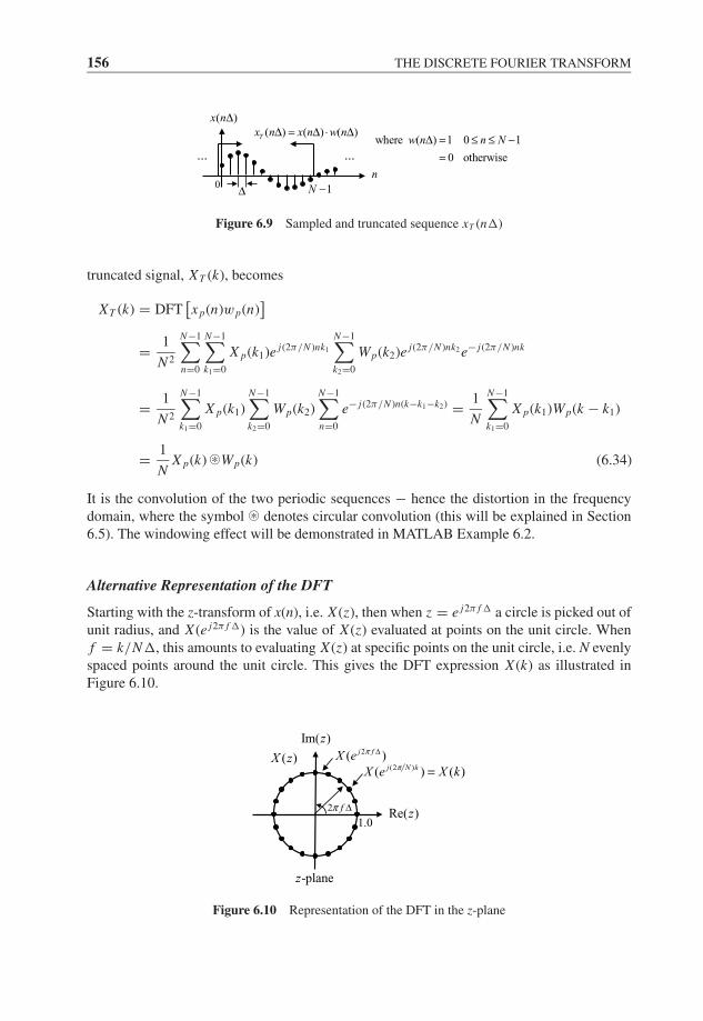
JWBK207-06 JWBK207-Shin January 26, 2008 18:29 Char Count= 0
156 THE DISCRETE FOURIER TRANSFORM
n
...
1N −Δ
( )x nΔ
...
0
( ) ( ) ( )Tx n x n w nΔ = Δ ⋅ Δwhere ( ) 1 0 1
0 otherwise
w n n NΔ = ≤ ≤ −=
Figure 6.9 Sampled and truncated sequence xT (n�)
truncated signal, XT (k), becomes
XT (k) = DFT[x p(n)wp(n)
]= 1
N 2
N−1∑n=0
N−1∑k1=0
X p(k1)e j(2π/N )nk1
N−1∑k2=0
Wp(k2)e j(2π/N )nk2 e− j(2π/N )nk
= 1
N 2
N−1∑k1=0
X p(k1)N−1∑k2=0
Wp(k2)N−1∑n=0
e− j(2π/N )n(k−k1−k2) = 1
N
N−1∑k1=0
X p(k1)Wp(k − k1)
= 1
NX p(k) ©* Wp(k) (6.34)
It is the convolution of the two periodic sequences − hence the distortion in the frequencydomain, where the symbol ©* denotes circular convolution (this will be explained in Section6.5). The windowing effect will be demonstrated in MATLAB Example 6.2.
Alternative Representation of the DFT
Starting with the z-transform of x(n), i.e. X (z), then when z = e j2π f � a circle is picked out ofunit radius, and X (e j2π f �) is the value of X (z) evaluated at points on the unit circle. Whenf = k/N�, this amounts to evaluating X (z) at specific points on the unit circle, i.e. N evenlyspaced points around the unit circle. This gives the DFT expression X (k) as illustrated inFigure 6.10.
2( )j fX e π Δ
(2 )( ) ( )j N kX e X kπ =( )X z
2 fπ Δ
Im( )z
1.0
-planez
Re( )z
Figure 6.10 Representation of the DFT in the z-plane
JWBK207-06 JWBK207-Shin January 26, 2008 18:29 Char Count= 0
THE DISCRETE FOURIER TRANSFORM 157
Frequency Resolution and Zero Padding
As we have seen earlier in Chapter 4, the frequency resolution of Fourier transform XT ( f )depends on the data length (or window length) T. Note that the data length of the truncatedsampled sequence xT (n�) is T = N�, and the frequency spacing in XT (k) is 1/N� =1/T Hz. Thus, we may have an arbitrary fine frequency spacing when T → ∞.
If the sequence x(n�) is finite in nature, then the Fourier transform of a sequenceX (e j2π f �) is fully representative of the original sequence without introducing truncation,because
X (e j2π f �) =∞∑
n=−∞x(n�)e− j2π f n� =
N−1∑n=0
x(n�)e− j2π f n�
Then, the DFT X (k) = X (e j2π f �)∣∣
f =k/N�gives the frequency spacing 1/N� Hz. This
spacing may be considered sufficient because we do not lose any information, i.e. we cancompletely recover x(n�) from X (k).
However, we often want to see more detail in the frequency domain, such as finer fre-quency spacing. A convenient procedure is simply to ‘add zeros’ to x(n), i.e. define
x(n) = x(n) 0 ≤ n ≤ N − 1
= 0 N ≤ n ≤ L − 1(6.35)
Then the L-point DFT of x(n) is
X (k) =L−1∑n=0
x(n)e− j(2π/L)nk =N−1∑n=0
x(n)e− j(2π/L)nk (6.36)
Thus, we see that X (k) = X (e j(2π/L)k), k = 0, 1, . . . , L − 1, i.e. ‘finer’ spacing round the unitcircle in the z-plane (see Figure 6.10), in other words, zero padding in the time domain resultsin the interpolation in the frequency domain (Smith, 2003). In vibration problems, this can beused to obtain the fine detail near resonances. However, care must be taken with this artificiallymade finer structure − the zero padding does not increase the ‘true’ resolution (see MATLABExample 4.6 in Chapter 4), i.e. the fundamental resolution is fixed and it is only the frequencyspacing that is reduced.
An interesting feature is that, with zero padding in the frequency domain, performing theinverse DFT results in interpolation in the time domain, i.e. an increased sampling rate in thetime domain (note that zeros are padded symmetrically with respect to N/2, and it is assumedthat X (N/2) = 0 for an even number of N). So zero padding in one domain results in a finerstructure in the other domain.
Zero padding is sometimes useful for analysing a transient signal that dies away quickly.For example, if we estimate the FRF of a system using the impact testing method, the measuredsignal (from the force sensor of an impact hammer) quickly falls into the noise level. In thiscase, we can artificially improve the quality of the measured signal by replacing the data inthe noise region with zeros (see MATLAB Example 6.7); note that the measurement time mayalso be increased (in effect) by adding more zeros. This approach can also be applied to thefree vibration signal of a highly damped system (see MATLAB Example 6.5).
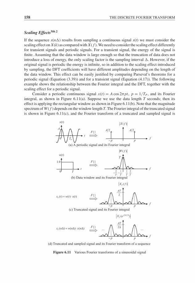
JWBK207-06 JWBK207-Shin January 26, 2008 18:29 Char Count= 0
158 THE DISCRETE FOURIER TRANSFORM
Scaling EffectsM6.2
If the sequence x(n�) results from sampling a continuous signal x(t) we must consider thescaling effect on X (k) as compared with X ( f ). We need to consider the scaling effect differentlyfor transient signals and periodic signals. For a transient signal, the energy of the signal isfinite. Assuming that the data window is large enough so that the truncation of data does notintroduce a loss of energy, the only scaling factor is the sampling interval �. However, if theoriginal signal is periodic the energy is infinite, so in addition to the scaling effect introducedby sampling, the DFT coefficients will have different amplitudes depending on the length ofthe data window. This effect can be easily justified by comparing Parseval’s theorems for aperiodic signal (Equation (3.39)) and for a transient signal (Equation (4.17)). The followingexample shows the relationship between the Fourier integral and the DFT, together with thescaling effect for a periodic signal.
Consider a periodic continuous signal x(t) = A cos 2πpt , p = 1/TP , and its Fourierintegral, as shown in Figure 6.11(a). Suppose we use the data length T seconds; then itseffect is applying the rectangular window as shown in Figure 6.11(b). Note that the magnitudespectrum of W ( f ) depends on the window length T. The Fourier integral of the truncated signalis shown in Figure 6.11(c), and the Fourier transform of a truncated and sampled signal is
(a) A periodic signal and its Fourier integral
(b) Data window and its Fourier integral
(c) Truncated signal and its Fourier integral
(d) Truncated and sampled signal and its Fourier transform of a sequence
f
{}F2A
( )X f
0 PTt
A
( )x t
2A
pp−
1
T
2
T
1
T−2
T−
( )W f
f
{}F1.0
( )w t
0 Tt
T
( ) ( ) ( )Tx t w t x t= ⋅
( )TX f
2
AT
f
{}F
pp−
2( )j fTX e π Δ
2
AT
Δ( ) ( ) ( )Tx n w n x nΔ = Δ ⋅ Δ ......
f
{}F
pp−
Figure 6.11 Various Fourier transforms of a sinusoidal signal
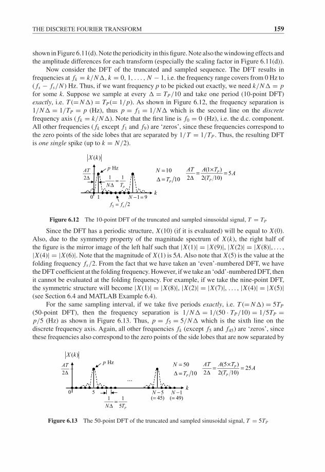
JWBK207-06 JWBK207-Shin January 26, 2008 18:29 Char Count= 0
THE DISCRETE FOURIER TRANSFORM 159
shown in Figure 6.11(d). Note the periodicity in this figure. Note also the windowing effects andthe amplitude differences for each transform (especially the scaling factor in Figure 6.11(d)).
Now consider the DFT of the truncated and sampled sequence. The DFT results infrequencies at fk = k/N�, k = 0, 1, . . . , N − 1, i.e. the frequency range covers from 0 Hz to( fs − fs/N ) Hz. Thus, if we want frequency p to be picked out exactly, we need k/N� = pfor some k. Suppose we sample at every � = TP/10 and take one period (10-point DFT)exactly, i.e. T (= N�) = TP (= 1/p). As shown in Figure 6.12, the frequency separation is1/N� = 1/TP = p (Hz), thus p = f1 = 1/N� which is the second line on the discretefrequency axis ( fk = k/N�). Note that the first line is f0 = 0 (Hz), i.e. the d.c. component.All other frequencies ( fk except f1 and f9) are ‘zeros’, since these frequencies correspond tothe zero points of the side lobes that are separated by 1/T = 1/TP . Thus, the resulting DFTis one single spike (up to k = N/2).
k
2
AT
Δ 1 1
PN T=
Δ
1 9N − =
10
10P
N
T
=Δ =
(1 )5
2 2( 10)P
P
A TATA
T
×= =Δ
( )X k
5 2sf f=
Hzp
10
Figure 6.12 The 10-point DFT of the truncated and sampled sinusoidal signal, T = TP
Since the DFT has a periodic structure, X (10) (if it is evaluated) will be equal to X (0).Also, due to the symmetry property of the magnitude spectrum of X (k), the right half ofthe figure is the mirror image of the left half such that |X (1)| = |X (9)|, |X (2)| = |X (8)|, . . . ,|X (4)| = |X (6)|. Note that the magnitude of X (1) is 5A. Also note that X (5) is the value at thefolding frequency fs/2. From the fact that we have taken an ‘even’-numbered DFT, we havethe DFT coefficient at the folding frequency. However, if we take an ‘odd’-numbered DFT, thenit cannot be evaluated at the folding frequency. For example, if we take the nine-point DFT,the symmetric structure will become |X (1)| = |X (8)|, |X (2)| = |X (7)|, . . . , |X (4)| = |X (5)|(see Section 6.4 and MATLAB Example 6.4).
For the same sampling interval, if we take five periods exactly, i.e. T (= N�) = 5TP
(50-point DFT), then the frequency separation is 1/N� = 1/(50 · TP/10) = 1/5TP =p/5 (Hz) as shown in Figure 6.13. Thus, p = f5 = 5/N� which is the sixth line on thediscrete frequency axis. Again, all other frequencies fk (except f5 and f45) are ‘zeros’, sincethese frequencies also correspond to the zero points of the side lobes that are now separated by
Hzp
...2
AT
Δ
1 1
5 PN T=
Δ
5( 45)N −=
50
10P
N
T
=Δ =
(5 )25
2 2( 10)P
P
A TATA
T
×= =Δ
1( 49)N −=
( )X k
0 5k
Figure 6.13 The 50-point DFT of the truncated and sampled sinusoidal signal, T = 5TP
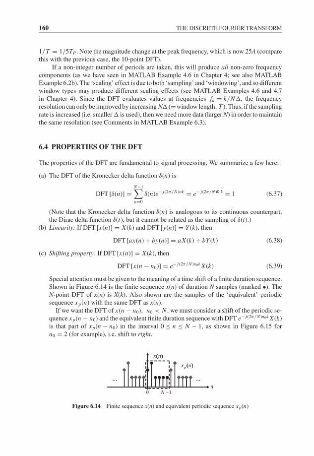
JWBK207-06 JWBK207-Shin January 26, 2008 18:29 Char Count= 0
160 THE DISCRETE FOURIER TRANSFORM
1/T = 1/5TP . Note the magnitude change at the peak frequency, which is now 25A (comparethis with the previous case, the 10-point DFT).
If a non-integer number of periods are taken, this will produce all non-zero frequencycomponents (as we have seen in MATLAB Example 4.6 in Chapter 4; see also MATLABExample 6.2b). The ‘scaling’ effect is due to both ‘sampling’ and ‘windowing’, and so differentwindow types may produce different scaling effects (see MATLAB Examples 4.6 and 4.7in Chapter 4). Since the DFT evaluates values at frequencies fk = k/N�, the frequencyresolution can only be improved by increasing N� (=window length, T ). Thus, if the samplingrate is increased (i.e. smaller � is used), then we need more data (larger N) in order to maintainthe same resolution (see Comments in MATLAB Example 6.3).
6.4 PROPERTIES OF THE DFT
The properties of the DFT are fundamental to signal processing. We summarize a few here:
(a) The DFT of the Kronecker delta function δ(n) is
DFT [δ(n)] =N−1∑n=0
δ(n)e− j(2π/N )nk = e− j(2π/N )0·k = 1 (6.37)
(Note that the Kronecker delta function δ(n) is analogous to its continuous counterpart,the Dirac delta function δ(t), but it cannot be related as the sampling of δ(t).)
(b) Linearity: If DFT [x(n)] = X (k) and DFT [y(n)] = Y (k), then
DFT [ax(n) + by(n)] = aX (k) + bY (k) (6.38)
(c) Shifting property: If DFT [x(n)] = X (k), then
DFT [x(n − n0)] = e− j(2π/N )n0k X (k) (6.39)
Special attention must be given to the meaning of a time shift of a finite duration sequence.Shown in Figure 6.14 is the finite sequence x(n) of duration N samples (marked •). TheN-point DFT of x(n) is X(k). Also shown are the samples of the ‘equivalent’ periodicsequence x p(n) with the same DFT as x(n).
If we want the DFT of x(n − n0), n0 < N , we must consider a shift of the periodic se-quence x p(n − n0) and the equivalent finite duration sequence with DFT e− j(2π/N )n0k X (k)is that part of x p(n − n0) in the interval 0 ≤ n ≤ N − 1, as shown in Figure 6.15 forn0 = 2 (for example), i.e. shift to right.
( )
( )x n
......n
( )px n
( )
0 1N −
Figure 6.14 Finite sequence x(n) and equivalent periodic sequence x p(n)
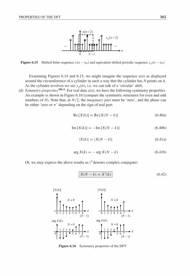
JWBK207-06 JWBK207-Shin January 26, 2008 18:29 Char Count= 0
PROPERTIES OF THE DFT 161
......
( 2)px n −
( 2)x n −
......
p −
−
0 1N −n
Figure 6.15 Shifted finite sequence x(n − n0) and equivalent shifted periodic sequence x p(n − n0)
Examining Figures 6.14 and 6.15, we might imagine the sequence x(n) as displayedaround the circumference of a cylinder in such a way that the cylinder has N points on it.As the cylinder revolves we see x p(n), i.e. we can talk of a ‘circular’ shift.
(d) Symmetry properties M6.4: For real data x(n), we have the following symmetry properties.An example is shown in Figure 6.16 (compare the symmetric structures for even and oddnumbers of N). Note that, at N/2, the imaginary part must be ‘zero’, and the phase canbe either ‘zero or π ’ depending on the sign of real part:
Re [X (k)] = Re [X (N − k)] (6.40a)
Im [X (k)] = −Im [X (N − k)] (6.40b)
|X (k)| = |X (N − k)| (6.41a)
arg X (k) = − arg X (N − k) (6.41b)
Or, we may express the above results as (*denotes complex conjugate)
X (N − k) = X∗(k) (6.42)
0
( )X k
(N − 1)1 2 3 4 5 6 7 8
k
9N =
0
( )X k
(N − 1)1 2 3 4 5 6 7
k
8N =
0
arg ( )X k
(N − 1)
1 2 3 4
5 6 7
8N =
k0
arg ( )X k
(N − 1)
1 2 3 4
5 6 7 8
9N =
k
Figure 6.16 Symmetry properties of the DFT
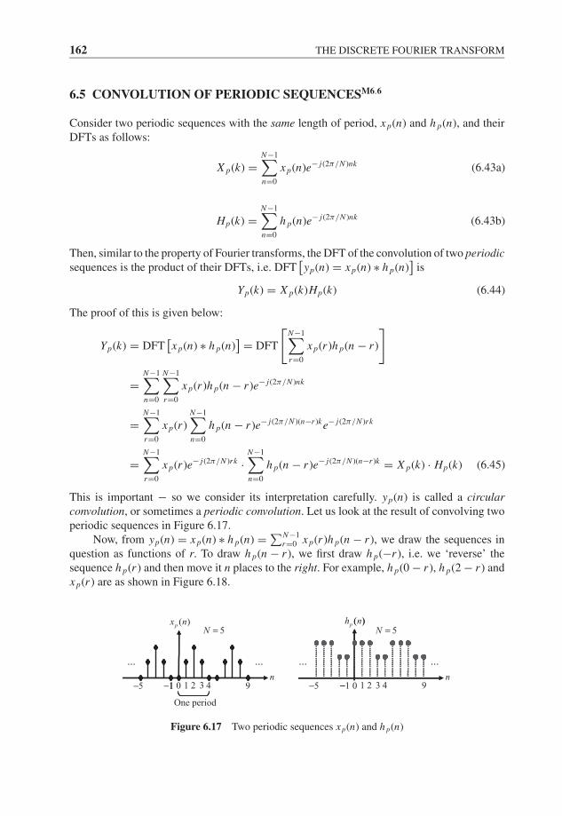
JWBK207-06 JWBK207-Shin January 26, 2008 18:29 Char Count= 0
162 THE DISCRETE FOURIER TRANSFORM
6.5 CONVOLUTION OF PERIODIC SEQUENCESM6.6
Consider two periodic sequences with the same length of period, x p(n) and h p(n), and theirDFTs as follows:
X p(k) =N−1∑n=0
x p(n)e− j(2π/N )nk (6.43a)
Hp(k) =N−1∑n=0
h p(n)e− j(2π/N )nk (6.43b)
Then, similar to the property of Fourier transforms, the DFT of the convolution of two periodicsequences is the product of their DFTs, i.e. DFT
[yp(n) = x p(n) ∗ h p(n)
]is
Yp(k) = X p(k)Hp(k) (6.44)
The proof of this is given below:
Yp(k) = DFT[x p(n) ∗ h p(n)
] = DFT
[N−1∑r=0
x p(r )h p(n − r )
]
=N−1∑n=0
N−1∑r=0
x p(r )h p(n − r )e− j(2π/N )nk
=N−1∑r=0
x p(r )N−1∑n=0
h p(n − r )e− j(2π/N )(n−r )ke− j(2π/N )rk
=N−1∑r=0
x p(r )e− j(2π/N )rk ·N−1∑n=0
h p(n − r )e− j(2π/N )(n−r )k = X p(k) · Hp(k) (6.45)
This is important − so we consider its interpretation carefully. yp(n) is called a circularconvolution, or sometimes a periodic convolution. Let us look at the result of convolving twoperiodic sequences in Figure 6.17.
Now, from yp(n) = x p(n) ∗ h p(n) = ∑N−1r=0 x p(r )h p(n − r ), we draw the sequences in
question as functions of r. To draw h p(n − r ), we first draw h p(−r ), i.e. we ‘reverse’ thesequence h p(r ) and then move it n places to the right. For example, h p(0 − r ), h p(2 − r ) andx p(r ) are as shown in Figure 6.18.
( )
1
( )h n
0−5
px n
......
n
5N =
One period
1 2 3 401−5− 9
( )
n
p
... ...
5N =
1 2 3 41−− 9
Figure 6.17 Two periodic sequences x p(n) and h p(n)
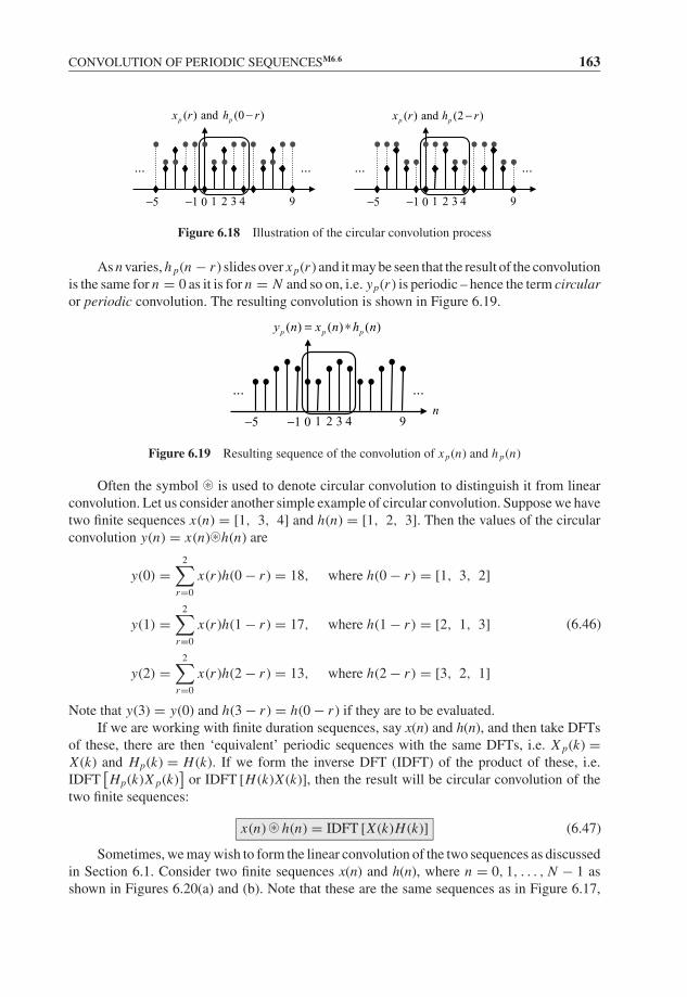
JWBK207-06 JWBK207-Shin January 26, 2008 18:29 Char Count= 0
CONVOLUTION OF PERIODIC SEQUENCESM6.6 163
...
( ) and (2 )p px r h r−
...
1 2 3 401−5− 9
( ) and (0 )p px r h r−
......
1 2 3 401−5− 9
Figure 6.18 Illustration of the circular convolution process
As n varies, h p(n − r ) slides over x p(r ) and it may be seen that the result of the convolutionis the same for n = 0 as it is for n = N and so on, i.e. yp(r ) is periodic – hence the term circularor periodic convolution. The resulting convolution is shown in Figure 6.19.
n
( ) ( ) ( )p p py n x n h n= ∗
......
1 2 3 401−5− 9
Figure 6.19 Resulting sequence of the convolution of x p(n) and h p(n)
Often the symbol ©* is used to denote circular convolution to distinguish it from linearconvolution. Let us consider another simple example of circular convolution. Suppose we havetwo finite sequences x(n) = [1, 3, 4] and h(n) = [1, 2, 3]. Then the values of the circularconvolution y(n) = x(n)©* h(n) are
y(0) =2∑
r=0
x(r )h(0 − r ) = 18, where h(0 − r ) = [1, 3, 2]
y(1) =2∑
r=0
x(r )h(1 − r ) = 17, where h(1 − r ) = [2, 1, 3]
y(2) =2∑
r=0
x(r )h(2 − r ) = 13, where h(2 − r ) = [3, 2, 1]
(6.46)
Note that y(3) = y(0) and h(3 − r ) = h(0 − r ) if they are to be evaluated.If we are working with finite duration sequences, say x(n) and h(n), and then take DFTs
of these, there are then ‘equivalent’ periodic sequences with the same DFTs, i.e. X p(k) =X (k) and Hp(k) = H (k). If we form the inverse DFT (IDFT) of the product of these, i.e.IDFT
[Hp(k)X p(k)
]or IDFT [H (k)X (k)], then the result will be circular convolution of the
two finite sequences:
x(n) ©* h(n) = IDFT [X (k)H (k)] (6.47)
Sometimes, we may wish to form the linear convolution of the two sequences as discussedin Section 6.1. Consider two finite sequences x(n) and h(n), where n = 0, 1, . . . , N − 1 asshown in Figures 6.20(a) and (b). Note that these are the same sequences as in Figure 6.17,
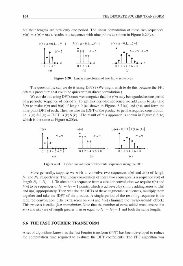
JWBK207-06 JWBK207-Shin January 26, 2008 18:29 Char Count= 0
164 THE DISCRETE FOURIER TRANSFORM
but their lengths are now only one period. The linear convolution of these two sequences,y(n) = x(n) ∗ h(n), results in a sequence with nine points as shown in Figure 6.20(c).
(c)
0
( ), 0,1, 1y n n L= −...,
1 2 3 4 5 6 7 8
2 1 9L N= − =
n
(b)
0
( ), 0,1, 1h n n N= −...,
1 2 3 4
5N =
n
(a)
0
( ), 0,1, 1x n n N= −...,
1 2 3 4
5N =
n
Figure 6.20 Linear convolution of two finite sequences
The question is: can we do it using DFTs? (We might wish to do this because the FFToffers a procedure that could be quicker than direct convolution.)
We can do this using DFTs once we recognize that the y(n) may be regarded as one periodof a periodic sequence of period 9. To get this periodic sequence we add zeros to x(n) andh(n) to make x(n) and h(n) of length 9 (as shown in Figures 6.21(a) and (b)), and form thenine-point DFT of each. Then we take the IDFT of the product to get the required convolution,i.e. x(n) ©* h(n) = IDFT [X (k)H (k)]. The result of this approach is shown in Figure 6.21(c)which is the same as Figure 6.20(c).
(c)
n
9N =
( )x n
0 1 2 3 4 5 6 7 8
)b()a(
( )h n
0 1 2 3 4 5 6 7 8
9N =
n0
[ ]( ) ( ) ( )y n IDFT X k H k=
1 2 3 4 5 6 7 8
9N =
n
Figure 6.21 Linear convolution of two finite sequences using the DFT
More generally, suppose we wish to convolve two sequences x(n) and h(n) of lengthN1 and N2, respectively. The linear convolution of these two sequences is a sequence y(n) oflength N1 + N2 − 1. To obtain this sequence from a circular convolution we require x(n) andh(n) to be sequences of N1 + N2 − 1 points, which is achieved by simply adding zeros to x(n)and h(n) appropriately. Then we take the DFTs of these augmented sequences, multiply themtogether and take the IDFT of the product. A single period of the resulting sequence is therequired convolution. (The extra zeros on x(n) and h(n) eliminate the ‘wrap-around’ effect.)This process is called fast convolution. Note that the number of zeros added must ensure thatx(n) and h(n) are of length greater than or equal to N1 + N2 − 1 and both the same length.
6.6 THE FAST FOURIER TRANSFORM
A set of algorithms known as the fast Fourier transform (FFT) has been developed to reducethe computation time required to evaluate the DFT coefficients. The FFT algorithm was
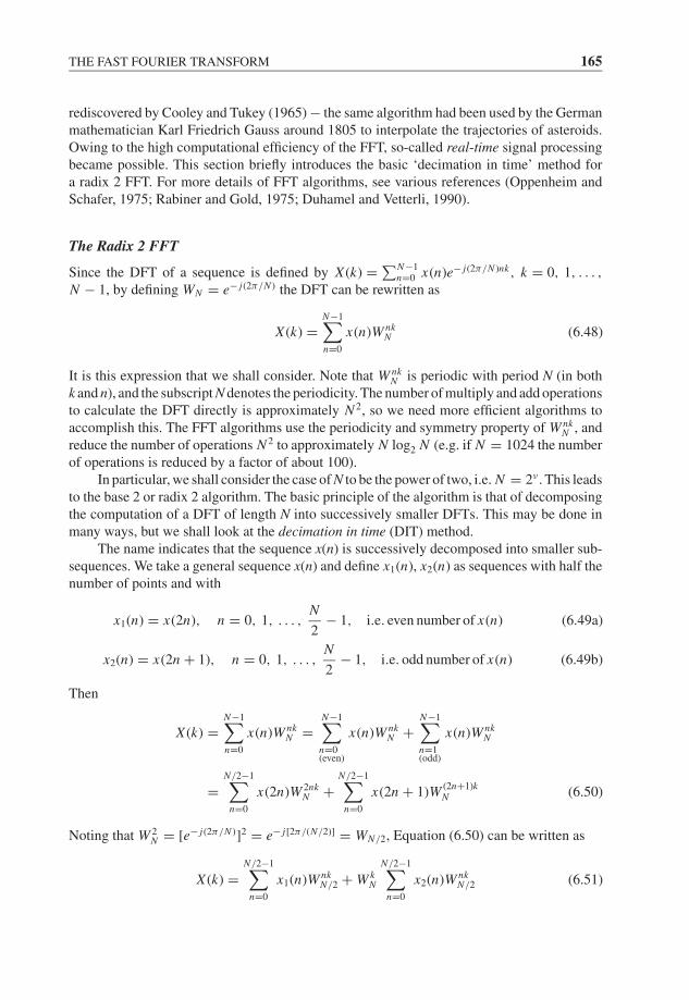
JWBK207-06 JWBK207-Shin January 26, 2008 18:29 Char Count= 0
THE FAST FOURIER TRANSFORM 165
rediscovered by Cooley and Tukey (1965) − the same algorithm had been used by the Germanmathematician Karl Friedrich Gauss around 1805 to interpolate the trajectories of asteroids.Owing to the high computational efficiency of the FFT, so-called real-time signal processingbecame possible. This section briefly introduces the basic ‘decimation in time’ method fora radix 2 FFT. For more details of FFT algorithms, see various references (Oppenheim andSchafer, 1975; Rabiner and Gold, 1975; Duhamel and Vetterli, 1990).
The Radix 2 FFT
Since the DFT of a sequence is defined by X (k) = ∑N−1n=0 x(n)e− j(2π/N )nk, k = 0, 1, . . . ,
N − 1, by defining WN = e− j(2π/N ) the DFT can be rewritten as
X (k) =N−1∑n=0
x(n)W nkN (6.48)
It is this expression that we shall consider. Note that W nkN is periodic with period N (in both
k and n), and the subscript N denotes the periodicity. The number of multiply and add operationsto calculate the DFT directly is approximately N 2, so we need more efficient algorithms toaccomplish this. The FFT algorithms use the periodicity and symmetry property of W nk
N , andreduce the number of operations N 2 to approximately N log2 N (e.g. if N = 1024 the numberof operations is reduced by a factor of about 100).
In particular, we shall consider the case of N to be the power of two, i.e. N = 2ν . This leadsto the base 2 or radix 2 algorithm. The basic principle of the algorithm is that of decomposingthe computation of a DFT of length N into successively smaller DFTs. This may be done inmany ways, but we shall look at the decimation in time (DIT) method.
The name indicates that the sequence x(n) is successively decomposed into smaller sub-sequences. We take a general sequence x(n) and define x1(n), x2(n) as sequences with half thenumber of points and with
x1(n) = x(2n), n = 0, 1, . . . ,N
2− 1, i.e. even number of x(n) (6.49a)
x2(n) = x(2n + 1), n = 0, 1, . . . ,N
2− 1, i.e. odd number of x(n) (6.49b)
Then
X (k) =N−1∑n=0
x(n)W nkN =
N−1∑n=0(even)
x(n)W nkN +
N−1∑n=1(odd)
x(n)W nkN
=N/2−1∑
n=0
x(2n)W 2nkN +
N/2−1∑n=0
x(2n + 1)W (2n+1)kN (6.50)
Noting that W 2N = [e− j(2π/N )]2 = e− j[2π/(N/2)] = WN/2, Equation (6.50) can be written as
X (k) =N/2−1∑
n=0
x1(n)W nkN/2 + W k
N
N/2−1∑n=0
x2(n)W nkN/2 (6.51)

JWBK207-06 JWBK207-Shin January 26, 2008 18:29 Char Count= 0
166 THE DISCRETE FOURIER TRANSFORM
i.e.
X (k) = X1(k) + W kN X2(k) (6.52)
where X1(k) and X2(k) are N/2-point DFTs of x1(n) and x2(n). Note that, since X (k) is definedfor 0 ≤ k ≤ N − 1 and X1(k), X2(k) are periodic with period N/2, then
X (k) = X1
(k − N
2
)+ W k
N X2
(k − N
2
)N
2≤ k ≤ N − 1 (6.53)
The above Equations (6.52) and (6.53) can be used to develop the computational procedure.For example, if N = 8 it can be shown that two four-pont DFTs are needed to make up thefull eight-point DFT. Now we do the same to the four-point DFT, i.e. divide x1(n) and x2(n)each into two sequences of even and odd numbers, e.g.
X1(k) = A(k) + W kN/2 B(k) = A(k) + W 2k
N B(k) for 0 ≤ k ≤ N
2− 1 (6.54)
where A(k) is a two-point DFT of even numbers of x1(n), and B(k) is a two-point DFT of oddnumbers of x1(n). This results in four two-pont DFTs in total. Thus, finally, we only need tocompute two-point DFTs.
In general, the total number of multiply and add operations is N log2 N . Finally, wecompare the number of operations N 2(DFT) versus N log2 N (FFT) in Table 6.1.
Table 6.1 Number of multiply and add operations, FFT versus DFT
N N 2 (DFT) N log2 N (FFT) N 2/(N log2 N )
16 256 64 4.0512 262 144 4608 56.9
2048 4 194 304 22 528 186.2
6.7 BRIEF SUMMARY
1. The input–output relationship of a digital LTI system is expressed by the convolutionof two sequences of h(n) and x(n), i.e.
y(n) =∞∑
k=−∞h(n − k)x(k) =
∞∑r=−∞
h(r )x(n − r ) or
y(n) = x(n) ∗ h(n) = h(n) ∗ x(n)
The Fourier transform of the sequence h(n), H (e j2π f ), is called the system frequencyresponse function (FRF), where
H (e j2π f ) =∞∑
n=−∞h(n)e− j2π f n and h(n) =
1/2∫−1/2
H (e j2π f )e j2π f nd f
Note that H (e j2π f ) is continuous and periodic in frequency.
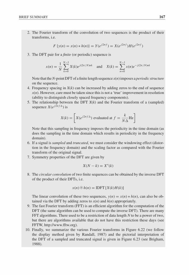
JWBK207-06 JWBK207-Shin January 26, 2008 18:29 Char Count= 0
BRIEF SUMMARY 167
2. The Fourier transform of the convolution of two sequences is the product of theirtransforms, i.e.
F {y(n) = x(n) ∗ h(n)} = Y (e j2π f ) = X (e j2π f )H (e j2π f )
3. The DFT pair for a finite (or periodic) sequence is
x(n) = 1
N
N−1∑k=0
X (k)e j(2π/N )nk and X (k) =N−1∑n=0
x(n)e− j(2π/N )nk
Note that the N-point DFT of a finite length sequence x(n) imposes a periodic structureon the sequence.
4. Frequency spacing in X(k) can be increased by adding zeros to the end of sequencex(n). However, care must be taken since this is not a ‘true’ improvement in resolution(ability to distinguish closely spaced frequency components).
5. The relationship between the DFT X(k) and the Fourier transform of a (sampled)sequence X (e j2π f �) is
X (k) =[
X (e j2π f �) evaluated at f = k
N�Hz
]Note that this sampling in frequency imposes the periodicity in the time domain (asdoes the sampling in the time domain which results in periodicity in the frequencydomain).
6. If a signal is sampled and truncated, we must consider the windowing effect (distor-tion in the frequency domain) and the scaling factor as compared with the Fouriertransform of the original signal.
7. Symmetry properties of the DFT are given by
X (N − k) = X∗(k)
8. The circular convolution of two finite sequences can be obtained by the inverse DFTof the product of their DFTs, i.e.
x(n) ©* h(n) = IDFT [X (k)H (k)]
The linear convolution of these two sequences, y(n) = x(n) ∗ h(n), can also be ob-tained via the DFT by adding zeros to x(n) and h(n) appropriately.
9. The fast Fourier transform (FFT) is an efficient algorithm for the computation of theDFT (the same algorithm can be used to compute the inverse DFT). There are manyFFT algorithms. There used to be a restriction of data length N to be a power of two,but there are algorithms available that do not have this restriction these days (seeFFTW, http://www.fftw.org).
10. Finally, we summarize the various Fourier transforms in Figure 6.22 (we followthe display method given by Randall, 1987) and the pictorial interpretation ofthe DFT of a sampled and truncated signal is given in Figure 6.23 (see Brigham,1988).
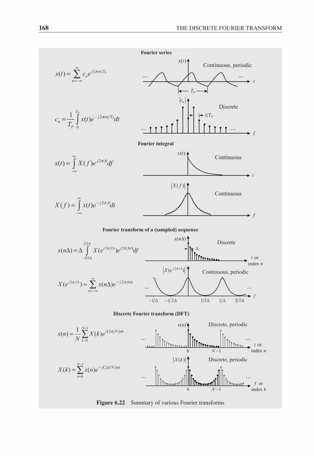
JWBK207-06 JWBK207-Shin January 26, 2008 18:29 Char Count= 0
168 THE DISCRETE FOURIER TRANSFORM
Fourier integral
f
( )X f
Continuous
2( ) ( ) j ftX f x t e dtπ∞
−
−∞
= ∫
( )x t
t
2( ) ( ) j ftx t X f e dfπ∞
−∞
= ∫Continuous
Fourier series
f
nc
1 PT
Discrete
2
0
1( )
P
P
Tj nt T
nP
c x t e dtT
π−= ∫......
PT
( )x t
t
Continuous, periodic2( ) Pj nt T
nn
x t c e π∞
=−∞= ∑ ......
Fourier transform of a (sampled) sequence
( )x nΔ
or
index
tn
Δ1 2
2 2
1 2
( ) ( )j f j fnx n X e e dfπ πΔ
Δ Δ
− Δ
Δ = Δ ∫Discrete
f
2( )j fX e π Δ
1 2Δ 1 Δ 3 2Δ1 2− Δ1− Δ
22( ) ( ) nfjfj
n
X e x n e ππ∞
Δ−Δ
=−∞= Δ∑
Continuous, periodic
......
Discrete Fourier transform (DFT)
( )x n
0 1N −
( )1
2
0
1( ) ( )
Nj N nk
k
x n X k eN
π−
== ∑
Discrete, periodic
or index
tn
......
( )X k
0 1N −
( )1
2
0
( ) ( )N
j N nk
n
X k x n e π−
−
== ∑
Discrete, periodic
or index
fk
......
Figure 6.22 Summary of various Fourier transforms
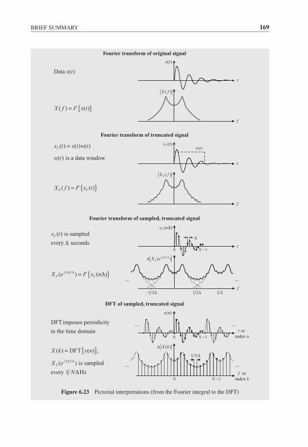
JWBK207-06 JWBK207-Shin January 26, 2008 18:29 Char Count= 0
BRIEF SUMMARY 169
Fourier transform of truncated signal
( )Tx t( )w t
t
( ) ( ) ( )
( ) is a data window
Tx t x t w t
w t
=
f
( )TX f
{ }( ) ( )T TX f F x t=
( )x t
t
Data ( )x t
f
( )X f
{ }( ) ( )X f F x t=
Fourier transform of original signal
Fourier transform of sampled, truncated signal
1N −
Δ
( )Tx nΔ
t0
( ) is sampled
every seconds
Tx t
Δ
f
2( )j fTX e π ΔΔ
1 2Δ 1 Δ1 2− Δ
{ }2( ) ( )j fTTX e F x nπ Δ = Δ
......
DFT of sampled, truncated signal
1N −
( )x n
0
DFT imposes periodicity
in the time domain or
index
tn
......
10 N −
( )X kΔ
1 NΔ[ ]( ) ( ) ,X k DFT x n=
2( ) is sampled
every 1 Hz
j fTX e
N
π Δ
Δ or index
fk
......
Figure 6.23 Pictorial interpretations (from the Fourier integral to the DFT)
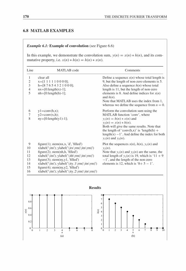
JWBK207-06 JWBK207-Shin January 26, 2008 18:29 Char Count= 0
170 THE DISCRETE FOURIER TRANSFORM
6.8 MATLAB EXAMPLES
Example 6.1: Example of convolution (see Figure 6.6)
In this example, we demonstrate the convolution sum, y(n) = x(n) ∗ h(n), and its com-mutative property, i.e. x(n) ∗ h(n) = h(n) ∗ x(n).
Line MATLAB code Comments
1 clear all Define a sequence x(n) whose total length is9, but the length of non-zero elements is 5.Also define a sequence h(n) whose totallength is 11, but the length of non-zeroelements is 8. And define indices for x(n)and h(n).Note that MATLAB uses the index from 1,whereas we define the sequence from n = 0.
2 x=[1 1 1 1 1 0 0 0 0];3 h=[8 7 6 5 4 3 2 1 0 0 0];4 nx=[0:length(x)-1];5 nh=[0:length(h)-1];
6 y1=conv(h,x);7 y2=conv(x,h);8 ny=[0:length(y1)-1];
Perform the convolution sum using theMATLAB function ‘conv’, wherey1(n) = h(n) ∗ x(n) andy2(n) = x(n) ∗ h(n).Both will give the same results. Note thatthe length of ‘conv(h,x)’ is ‘length(h) +length(x) −1’. And define the index for bothy1(n) and y2(n).
9 figure(1); stem(nx,x, 'd', 'filled') Plot the sequences x(n), h(n), y1(n) andy2(n).Note that y1(n) and y2(n) are the same, thetotal length of y1(n) is 19, which is ‘11 + 9−1’, and the length of the non-zeroelements is 12, which is ‘8+ 5 − 1’.
10 xlabel('\itn'); ylabel('\itx\rm(\itn\rm)')11 figure(2); stem(nh,h, 'filled')12 xlabel('\itn'); ylabel('\ith\rm(\itn\rm)')13 figure(3); stem(ny,y1, 'filled')14 xlabel('\itn'); ylabel('\ity 1\rm(\itn\rm)')15 figure(4); stem(ny,y2, 'filled')16 xlabel('\itn'); ylabel('\ity 2\rm(\itn\rm)')
Results
x(n)
0 1 2 3 4 5 6 7 80
0.2
0.4
0.6
0.8
1
n
(a)
0 1 2 3 4 5 6 7 8 9 100
1
2
3
4
5
6
7
8
n
h(n)
(b)
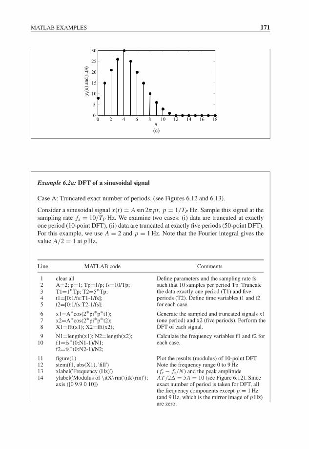
JWBK207-06 JWBK207-Shin January 26, 2008 18:29 Char Count= 0
MATLAB EXAMPLES 171
y 1(n
) an
d y
2(n
)
0 2 4 6 8 10 12 14 16 180
5
10
15
20
25
30
n(c)
Example 6.2a: DFT of a sinusoidal signal
Case A: Truncated exact number of periods. (see Figures 6.12 and 6.13).
Consider a sinusoidal signal x(t) = A sin 2πpt , p = 1/TP Hz. Sample this signal at thesampling rate fs = 10/TP Hz. We examine two cases: (i) data are truncated at exactlyone period (10-point DFT), (ii) data are truncated at exactly five periods (50-point DFT).For this example, we use A = 2 and p = 1 Hz. Note that the Fourier integral gives thevalue A/2 = 1 at p Hz.
Line MATLAB code Comments
1 clear all Define parameters and the sampling rate fssuch that 10 samples per period Tp. Truncatethe data exactly one period (T1) and fiveperiods (T2). Define time variables t1 and t2for each case.
2 A=2; p=1; Tp=1/p; fs=10/Tp;3 T1=1*Tp; T2=5*Tp;4 t1=[0:1/fs:T1-1/fs];5 t2=[0:1/fs:T2-1/fs];
6 x1=A*cos(2*pi*p*t1); Generate the sampled and truncated signals x1(one period) and x2 (five periods). Perform theDFT of each signal.
7 x2=A*cos(2*pi*p*t2);8 X1=fft(x1); X2=fft(x2);
9 N1=length(x1); N2=length(x2); Calculate the frequency variables f1 and f2 foreach case.10 f1=fs*(0:N1-1)/N1;
f2=fs*(0:N2-1)/N2;
11 figure(1) Plot the results (modulus) of 10-point DFT.Note the frequency range 0 to 9 Hz( fs − fs/N ) and the peak amplitudeAT /2� = 5A = 10 (see Figure 6.12). Sinceexact number of period is taken for DFT, allthe frequency components except p = 1 Hz(and 9 Hz, which is the mirror image of p Hz)are zero.
12 stem(f1, abs(X1), 'fill')13 xlabel('Frequency (Hz)')14 ylabel('Modulus of \itX\rm(\itk\rm)');
axis ([0 9.9 0 10])

JWBK207-06 JWBK207-Shin January 26, 2008 18:29 Char Count= 0
172 THE DISCRETE FOURIER TRANSFORM
15 figure(2) This plots the same results, but now theDFT coefficients are scaled appropriately.Note that the modulus of X(k) is dividedby the sampling rate (fs) and windowlength (T1). Note that it also givesthe same scaling effect if X(k) is dividedby the number of points N1. The resultcorresponds to the Fourier integral, i.e. thepeak amplitude is now A/2 = 1 at p Hz.
16 stem(f1, abs(X1)/fs/T1, 'fill'); % this is thesame as stem(f1, abs(X1)/N1, 'fill')
17 xlabel('Frequency (Hz)')18 ylabel('Modulus (scaled)');
axis ([0 9.9 0 1])
19202122
figure(3)stem(f2, abs(X2), 'fill')xlabel('Frequency (Hz)')ylabel('Modulus of \itX\rm(\itk\rm)')
Plot the results (modulus) of 50-pointDFT. Note that the peak amplitude isAT /2� = 25A = 50. In this case, weused the data five times longer in ‘time’than in the previous case. This results inan increase of frequency resolution, i.e.the resolution is increased five times thatin the previous case.
23 figure(4) This plots the same results, but, as before,the DFT coefficients are scaledappropriately, thus A/2 = 1 at p Hz.
24 stem(f2, abs(X2)/fs/T2, 'fill'); % this is thesame as stem(f2, abs(X2)/N2, 'fill')
25 xlabel('Frequency (Hz)');ylabel('Modulus (scaled)')
Results
0 1 2 3 4 5 6 7 8 90
1
2
3
4
5
6
7
8
9
10
Frequency (Hz)
Modulu
s of
X(k
)
2 , ( 2)sN f 1, ( )s sN f f N− −
5 10A =
1 Hzp =
10N = (a1)
0 1 2 3 4 5 6 7 8 90
0.1
0.2
0.3
0.4
0.5
0.6
0.7
0.8
0.9
1
Frequency (Hz)
Modulu
s (s
cale
d)
Magnitude is scaled appropriately
10N = (a2)
Modulu
s of
X(k
)
0 1 2 3 4 5 6 7 8 9 100
5
10
15
20
25
30
35
40
45
50
Frequency (Hz)
2, ( 2)sN f 1, ( )s sN f f N− −
25 50A =
1 Hzp =
50N = (a3)
0 1 2 3 4 5 6 7 8 9 100
0.1
0.2
0.3
0.4
0.5
0.6
0.7
0.8
0.9
1
Frequency (Hz)
Modulu
s (s
cale
d)
Magnitude is scaled appropriately
50N = (a4)
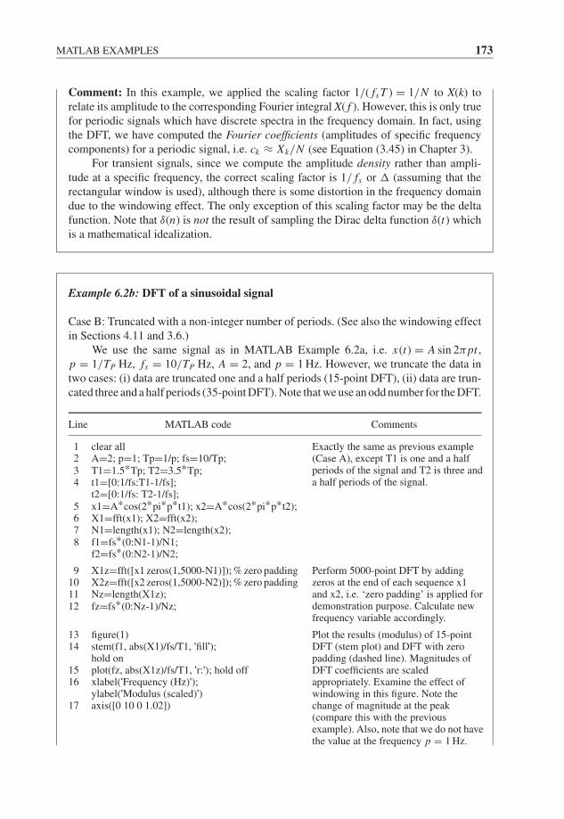
JWBK207-06 JWBK207-Shin January 26, 2008 18:29 Char Count= 0
MATLAB EXAMPLES 173
Comment: In this example, we applied the scaling factor 1/( fs T ) = 1/N to X(k) torelate its amplitude to the corresponding Fourier integral X( f ). However, this is only truefor periodic signals which have discrete spectra in the frequency domain. In fact, usingthe DFT, we have computed the Fourier coefficients (amplitudes of specific frequencycomponents) for a periodic signal, i.e. ck ≈ Xk/N (see Equation (3.45) in Chapter 3).
For transient signals, since we compute the amplitude density rather than ampli-tude at a specific frequency, the correct scaling factor is 1/ fs or � (assuming that therectangular window is used), although there is some distortion in the frequency domaindue to the windowing effect. The only exception of this scaling factor may be the deltafunction. Note that δ(n) is not the result of sampling the Dirac delta function δ(t) whichis a mathematical idealization.
Example 6.2b: DFT of a sinusoidal signal
Case B: Truncated with a non-integer number of periods. (See also the windowing effectin Sections 4.11 and 3.6.)
We use the same signal as in MATLAB Example 6.2a, i.e. x(t) = A sin 2πpt ,p = 1/TP Hz, fs = 10/TP Hz, A = 2, and p = 1 Hz. However, we truncate the data intwo cases: (i) data are truncated one and a half periods (15-point DFT), (ii) data are trun-cated three and a half periods (35-point DFT). Note that we use an odd number for the DFT.
Line MATLAB code Comments
1 clear all Exactly the same as previous example(Case A), except T1 is one and a halfperiods of the signal and T2 is three anda half periods of the signal.
2 A=2; p=1; Tp=1/p; fs=10/Tp;3 T1=1.5*Tp; T2=3.5*Tp;4 t1=[0:1/fs:T1-1/fs];
t2=[0:1/fs: T2-1/fs];5 x1=A*cos(2*pi*p*t1); x2=A*cos(2*pi*p*t2);6 X1=fft(x1); X2=fft(x2);7 N1=length(x1); N2=length(x2);8 f1=fs*(0:N1-1)/N1;
f2=fs*(0:N2-1)/N2;
9 X1z=fft([x1 zeros(1,5000-N1)]); % zero padding Perform 5000-point DFT by addingzeros at the end of each sequence x1and x2, i.e. ‘zero padding’ is applied fordemonstration purpose. Calculate newfrequency variable accordingly.
10 X2z=fft([x2 zeros(1,5000-N2)]); % zero padding11 Nz=length(X1z);12 fz=fs*(0:Nz-1)/Nz;
13 figure(1) Plot the results (modulus) of 15-pointDFT (stem plot) and DFT with zeropadding (dashed line). Magnitudes ofDFT coefficients are scaledappropriately. Examine the effect ofwindowing in this figure. Note thechange of magnitude at the peak(compare this with the previousexample). Also, note that we do not havethe value at the frequency p = 1 Hz.
14 stem(f1, abs(X1)/fs/T1, 'fill');hold on
15 plot(fz, abs(X1z)/fs/T1, 'r:'); hold off16 xlabel('Frequency (Hz)');
ylabel('Modulus (scaled)')17 axis([0 10 0 1.02])
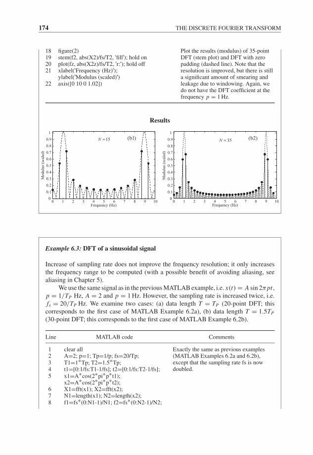
JWBK207-06 JWBK207-Shin January 26, 2008 18:29 Char Count= 0
174 THE DISCRETE FOURIER TRANSFORM
18 figure(2) Plot the results (modulus) of 35-pointDFT (stem plot) and DFT with zeropadding (dashed line). Note that theresolution is improved, but there is stilla significant amount of smearing andleakage due to windowing. Again, wedo not have the DFT coefficient at thefrequency p = 1 Hz.
19 stem(f2, abs(X2)/fs/T2, 'fill'); hold on20 plot(fz, abs(X2z)/fs/T2, 'r:'); hold off21 xlabel('Frequency (Hz)');
ylabel('Modulus (scaled)')22 axis([0 10 0 1.02])
Results
0 1 2 3 4 5 6 7 8 9 100
0.1
0.2
0.3
0.4
0.5
0.6
0.7
0.8
0.9
1
Frequency (Hz)
Mo
du
lus
(sca
led
)
15N = (b1) 35N =
0 1 2 3 4 5 6 7 8 9 100
0.1
0.2
0.3
0.4
0.5
0.6
0.7
0.8
0.9
1
Frequency (Hz)
Mo
du
lus
(sca
led
)
(b2)
Example 6.3: DFT of a sinusoidal signal
Increase of sampling rate does not improve the frequency resolution; it only increasesthe frequency range to be computed (with a possible benefit of avoiding aliasing, seealiasing in Chapter 5).
We use the same signal as in the previous MATLAB example, i.e. x(t) = A sin 2πpt ,p = 1/TP Hz, A = 2 and p = 1 Hz. However, the sampling rate is increased twice, i.e.fs = 20/TP Hz. We examine two cases: (a) data length T = TP (20-point DFT; thiscorresponds to the first case of MATLAB Example 6.2a), (b) data length T = 1.5TP
(30-point DFT; this corresponds to the first case of MATLAB Example 6.2b).
Line MATLAB code Comments
1 clear all Exactly the same as previous examples(MATLAB Examples 6.2a and 6.2b),except that the sampling rate fs is nowdoubled.
2 A=2; p=1; Tp=1/p; fs=20/Tp;3 T1=1*Tp; T2=1.5*Tp;4 t1=[0:1/fs:T1-1/fs]; t2=[0:1/fs:T2-1/fs];5 x1=A*cos(2*pi*p*t1);
x2=A*cos(2*pi*p*t2);6 X1=fft(x1); X2=fft(x2);7 N1=length(x1); N2=length(x2);8 f1=fs*(0:N1-1)/N1; f2=fs*(0:N2-1)/N2;
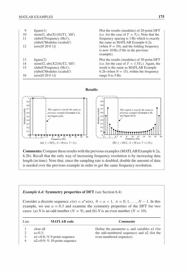
JWBK207-06 JWBK207-Shin January 26, 2008 18:29 Char Count= 0
MATLAB EXAMPLES 175
9 figure(1) Plot the results (modulus) of 20-point DFT(i.e. for the case of T = TP ). Note that thefrequency spacing is 1 Hz which is exactlythe same as MATLAB Example 6.2a(when N = 10), and the folding frequencyis now 10 Hz (5 Hz in the previousexample).
10 stem(f1, abs(X1)/fs/T1, 'fill')11 xlabel('Frequency (Hz)');
ylabel('Modulus (scaled)')12 axis([0 20 0 1])
13 figure(2) Plot the results (modulus) of 30-point DFT(i.e. for the case of T = 1.5TP ). Again, theresult is the same as MATLAB Example6.2b (when N = 15), within the frequencyrange 0 to 5 Hz.
14 stem(f2, abs(X2)/fs/T2, 'fill')15 xlabel('Frequency (Hz)');
ylabel('Modulus (scaled)')16 axis([0 20 0 1])
Results
20 , 20 (i.e. )(a) PPsf T N T T= = =
0 2 4 6 8 10 12 14 16 18 200
0.1
0.2
0.3
0.4
0.5
0.6
0.7
0.8
0.9
1
Frequency (Hz)
Modulu
s (s
cale
d) This region is exactly the same as
previous example (Example 6.2a,
see Figure (a2))
This region is exactly the same as previous example (Example 6.2b, see Figure (b1))
0 2 4 6 8 10 12 14 16 18 200
0.1
0.2
0.3
0.4
0.5
0.6
0.7
0.8
0.9
1
Frequency (Hz)
Modulu
s (s
cale
d)
20 , 30 (i.e. 1.5 )(b) PPsf T N T T= = =
Comments: Compare these results with the previous examples (MATLAB Example 6.2a,6.2b). Recall that the only way of increasing frequency resolution is by increasing datalength (in time). Note that, since the sampling rate is doubled, double the amount of datais needed over the previous example in order to get the same frequency resolution.
Example 6.4: Symmetry properties of DFT (see Section 6.4)
Consider a discrete sequence x(n) = anu(n), 0 < a < 1, n = 0, 1, . . . , N − 1. In thisexample, we use a = 0.3 and examine the symmetry properties of the DFT for twocases: (a) N is an odd number (N = 9), and (b) N is an even number (N = 10).
Line MATLAB code Comments
1 clear all Define the parameter a, and variables n1 (forthe odd-numbered sequence) and n2 (for theeven-numbered sequence).
2 a=0.3;3 n1=0:8; % 9-point sequence4 n2=0:9; % 10-point sequence
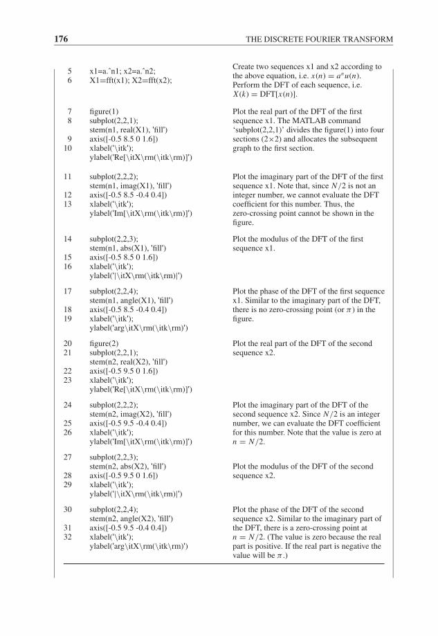
JWBK207-06 JWBK207-Shin January 26, 2008 18:29 Char Count= 0
176 THE DISCRETE FOURIER TRANSFORM
5 x1=a.ˆn1; x2=a.ˆn2;Create two sequences x1 and x2 according tothe above equation, i.e. x(n) = anu(n).Perform the DFT of each sequence, i.e.X (k) = DFT[x(n)].
6 X1=fft(x1); X2=fft(x2);
7 figure(1) Plot the real part of the DFT of the firstsequence x1. The MATLAB command‘subplot(2,2,1)’ divides the figure(1) into foursections (2×2) and allocates the subsequentgraph to the first section.
8 subplot(2,2,1);stem(n1, real(X1), 'fill')
9 axis([-0.5 8.5 0 1.6])10 xlabel('\itk');
ylabel('Re[\itX\rm(\itk\rm)]')
11 subplot(2,2,2);stem(n1, imag(X1), 'fill')
Plot the imaginary part of the DFT of the firstsequence x1. Note that, since N/2 is not aninteger number, we cannot evaluate the DFTcoefficient for this number. Thus, thezero-crossing point cannot be shown in thefigure.
12 axis([-0.5 8.5 -0.4 0.4])13 xlabel('\itk');
ylabel('Im[\itX\rm(\itk\rm)]')
14 subplot(2,2,3);stem(n1, abs(X1), 'fill')
Plot the modulus of the DFT of the firstsequence x1.
15 axis([-0.5 8.5 0 1.6])16 xlabel('\itk');
ylabel('|\itX\rm(\itk\rm)|')17 subplot(2,2,4);
stem(n1, angle(X1), 'fill')Plot the phase of the DFT of the first sequencex1. Similar to the imaginary part of the DFT,there is no zero-crossing point (or π ) in thefigure.
18 axis([-0.5 8.5 -0.4 0.4])19 xlabel('\itk');
ylabel('arg\itX\rm(\itk\rm)')
20 figure(2) Plot the real part of the DFT of the secondsequence x2.21 subplot(2,2,1);
stem(n2, real(X2), 'fill')22 axis([-0.5 9.5 0 1.6])23 xlabel('\itk');
ylabel('Re[\itX\rm(\itk\rm)]')
24 subplot(2,2,2);stem(n2, imag(X2), 'fill')
Plot the imaginary part of the DFT of thesecond sequence x2. Since N/2 is an integernumber, we can evaluate the DFT coefficientfor this number. Note that the value is zero atn = N/2.
25 axis([-0.5 9.5 -0.4 0.4])26 xlabel('\itk');
ylabel('Im[\itX\rm(\itk\rm)]')
27 subplot(2,2,3);stem(n2, abs(X2), 'fill') Plot the modulus of the DFT of the second
sequence x2.28 axis([-0.5 9.5 0 1.6])29 xlabel('\itk');
ylabel('|\itX\rm(\itk\rm)|')30 subplot(2,2,4);
stem(n2, angle(X2), 'fill')Plot the phase of the DFT of the secondsequence x2. Similar to the imaginary part ofthe DFT, there is a zero-crossing point atn = N/2. (The value is zero because the realpart is positive. If the real part is negative thevalue will be π .)
31 axis([-0.5 9.5 -0.4 0.4])32 xlabel('\itk');
ylabel('arg\itX\rm(\itk\rm)')
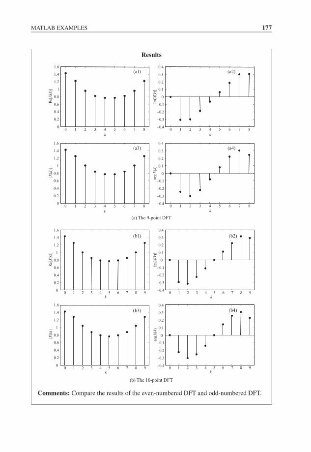
JWBK207-06 JWBK207-Shin January 26, 2008 18:29 Char Count= 0
MATLAB EXAMPLES 177
Results
0 1 2 3 4 5 6 7 80
0.2
0.4
0.6
0.8
1
1.2
1.4
1.6
k
Re[
X(k
)]
(a1)
0 1 2 3 4 5 6 7 8–0.4
–0.3
–0.2
–0.1
0
0.1
0.2
0.3
0.4
k
Im[X
(k)]
(a2)
(a) The 9-point DFT
0 1 2 3 4 5 6 7 80
0.2
0.4
0.6
0.8
1
1.2
1.4
1.6
k
|X(k
)|
(a3)
0 1 2 3 4 5 6 7 8–0.4
–0.3
–0.2
–0.1
0
0.1
0.2
0.3
0.4
k
arg
X(k
)
(a4)
Re[
X(k
)]
0 1 2 3 4 5 6 7 8 90
0.2
0.4
0.6
0.8
1
1.2
1.4
1.6
k
(b1)
Im[X
(k)]
0 1 2 3 4 5 6 7 8 9–0.4
–0.3
–0.2
–0.1
0
0.1
0.2
0.3
0.4
k
(b2)
|X(k
)|
0 1 2 3 4 5 6 7 8 90
0.2
0.4
0.6
0.8
1
1.2
1.4
1.6
k
(b3)
arg
X(k
)
0 1 2 3 4 5 6 7 8 9–0.4
–0.3
–0.2
–0.1
0
0.1
0.2
0.3
0.4
k
(b4)
(b) The 10-point DFT
Comments: Compare the results of the even-numbered DFT and odd-numbered DFT.
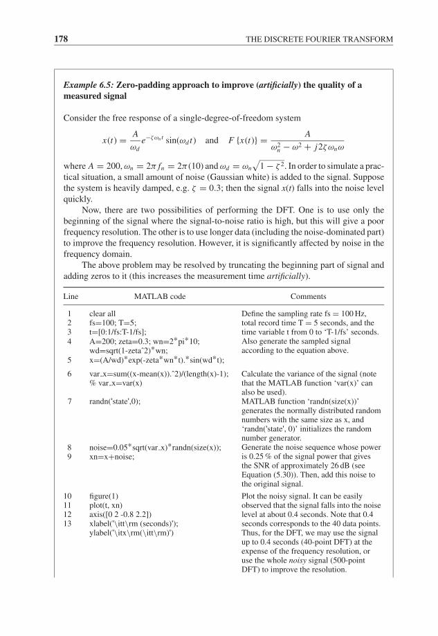
JWBK207-06 JWBK207-Shin January 26, 2008 18:29 Char Count= 0
178 THE DISCRETE FOURIER TRANSFORM
Example 6.5: Zero-padding approach to improve (artificially) the quality of ameasured signal
Consider the free response of a single-degree-of-freedom system
x(t) = A
ωde−ζωn t sin(ωd t) and F {x(t)} = A
ω2n − ω2 + j2ζωnω
where A = 200, ωn = 2π fn = 2π (10) and ωd = ωn
√1 − ζ 2. In order to simulate a prac-
tical situation, a small amount of noise (Gaussian white) is added to the signal. Supposethe system is heavily damped, e.g. ζ = 0.3; then the signal x(t) falls into the noise levelquickly.
Now, there are two possibilities of performing the DFT. One is to use only thebeginning of the signal where the signal-to-noise ratio is high, but this will give a poorfrequency resolution. The other is to use longer data (including the noise-dominated part)to improve the frequency resolution. However, it is significantly affected by noise in thefrequency domain.
The above problem may be resolved by truncating the beginning part of signal andadding zeros to it (this increases the measurement time artificially).
Line MATLAB code Comments
1 clear all Define the sampling rate fs = 100 Hz,total record time T = 5 seconds, and thetime variable t from 0 to ‘T-1/fs’ seconds.Also generate the sampled signalaccording to the equation above.
2 fs=100; T=5;3 t=[0:1/fs:T-1/fs];4 A=200; zeta=0.3; wn=2*pi*10;
wd=sqrt(1-zetaˆ2)*wn;5 x=(A/wd)*exp(-zeta*wn*t).*sin(wd*t);
6 var x=sum((x-mean(x)).ˆ2)/(length(x)-1);% var x=var(x)
7 randn('state',0);
Calculate the variance of the signal (notethat the MATLAB function ‘var(x)’ canalso be used).MATLAB function ‘randn(size(x))’generates the normally distributed randomnumbers with the same size as x, and‘randn('state', 0)’ initializes the randomnumber generator.Generate the noise sequence whose poweris 0.25 % of the signal power that givesthe SNR of approximately 26 dB (seeEquation (5.30)). Then, add this noise tothe original signal.
8 noise=0.05*sqrt(var x)*randn(size(x));9 xn=x+noise;
10 figure(1) Plot the noisy signal. It can be easilyobserved that the signal falls into the noiselevel at about 0.4 seconds. Note that 0.4seconds corresponds to the 40 data points.Thus, for the DFT, we may use the signalup to 0.4 seconds (40-point DFT) at theexpense of the frequency resolution, oruse the whole noisy signal (500-pointDFT) to improve the resolution.
11 plot(t, xn)12 axis([0 2 -0.8 2.2])13 xlabel('\itt\rm (seconds)');
ylabel('\itx\rm(\itt\rm)')

JWBK207-06 JWBK207-Shin January 26, 2008 18:29 Char Count= 0
MATLAB EXAMPLES 179
14 Xn1=fft(xn,40); % 40 corresponds to0.4 seconds in time
First, perform the DFT using only the first40 data points of the signal. TheMATLAB function ‘fft(xn, 40)’ performsthe DFT of xn using the first 40 elementsof xn. Next, perform the DFT using thewhole noisy signal (500-point DFT).Calculate the corresponding frequencyvariables.
15 N1=length(Xn1);f1=fs*(0:N1-1)/N1;
16 Xn2=fft(xn);17 N2=length(xn);
f2=fs*(0:N2-1)/N2;
18 Xa=A./(wnˆ2 - (2*pi*f2).ˆ2 +i*2*zeta*wn*(2*pi*f2));
Calculate the Fourier integral according tothe formula above. This will be used forthe purpose of comparison.
19 figure(2) Plot the modulus of the 40-point DFT(solid line), and plot the true magnitudespectrum of the Fourier transform (dashedline). Note the poor frequency resolutionin the case of the 40-point DFT.
20 plot(f1(1:N1/2+1),20*log10(abs(Xn1(1:N1/2 +1)/fs)))
21 hold on22 plot(f2(1:N2/2+1),
20*log10(abs(Xa(1:N2/2+1))), 'r:')23 xlabel('Frequency (Hz)');
ylabel('Modulus (dB)'); hold off
24 figure(3) Plot the modulus of the DFT of the wholenoisy signal (solid line), and plot the truemagnitude spectrum of the Fouriertransform (dashed line). Note the effect ofnoise in the frequency domain.
25 plot(f2(1:N2/2+1),20*log10(abs(Xn2(1:N2/2+1)/fs)))
26 hold on27 plot(f2(1:N2/2+1),
20*log10(abs(Xa(1:N2/2+1))), 'r:')28 xlabel('Frequency (Hz)');
ylabel('Modulus (dB)'); hold off
29 Xnz=fft(xn(1:40),N2); Now, perform the DFT of the truncatedand zero-padded signal. The MATLABfunction ‘fft(xn(1:40),N2)’ takes only thefirst 40 data elements of xn, then addszeros up to the number N2.
30 figure(4) Plot the modulus of the DFT of thezero-padded signal (solid line), and plotthe true magnitude spectrum of theFourier transform (dashed line). Note theimprovement in the frequency domain.
31 plot(f2(1:N2/2+1),20*log10(abs(Xnz(1:N2/2+1)/fs)))
32 hold on33 plot(f2(1:N2/2+1),
20*log10(abs(Xa(1:N2/2+1))), 'r:')34 xlabel('Frequency (Hz)');
ylabel('Modulus (dB)'); hold off
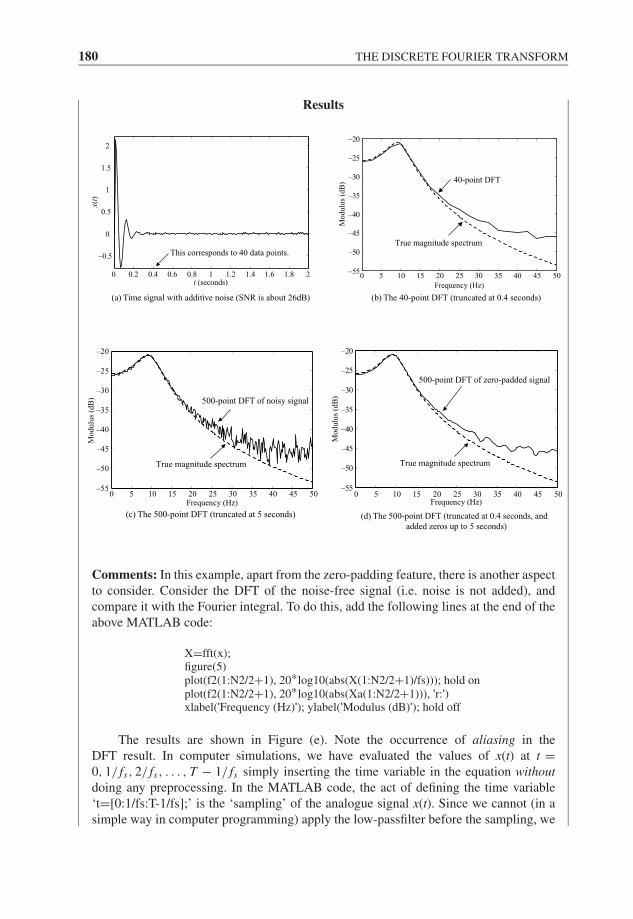
JWBK207-06 JWBK207-Shin January 26, 2008 18:29 Char Count= 0
180 THE DISCRETE FOURIER TRANSFORM
Results
0 0.2 0.4 0.6 0.8 1 1.2 1.4 1.6 1.8 2
–0.5
0
0.5
1
1.5
2
t (seconds)
x(t)
This corresponds to 40 data points.
(a) Time signal with additive noise (SNR is about 26dB)
0 5 10 15 20 25 30 35 40 45 50–55
–50
–45
–40
–35
–30
–25
–20
Frequency (Hz)
Modulu
s (d
B) 40-point DFT
True magnitude spectrum
(b) The 40-point DFT (truncated at 0.4 seconds)
0 5 10 15 20 25 30 35 40 45 50–55
–50
–45
–40
–35
–30
–25
–20
Frequency (Hz)
Modulu
s (d
B) 500-point DFT
(c) The 500-point DFT (truncated at 5 seconds)
of noisy signal
True magnitude spectrum
500-point DFT of zero-padded signal
T
(d) The 500-point DFT (truncated at 0.4 seconds, and added zeros up to 5 seconds)
rue magnitude spectrum
0 5 10 15 20 25 30 35 40 45 50–55
–50
–45
–40
–35
–30
–25
–20
Frequency (Hz)
Modulu
s (d
B)
Comments: In this example, apart from the zero-padding feature, there is another aspectto consider. Consider the DFT of the noise-free signal (i.e. noise is not added), andcompare it with the Fourier integral. To do this, add the following lines at the end of theabove MATLAB code:
X=fft(x);figure(5)plot(f2(1:N2/2+1), 20*log10(abs(X(1:N2/2+1)/fs))); hold onplot(f2(1:N2/2+1), 20*log10(abs(Xa(1:N2/2+1))), 'r:')xlabel('Frequency (Hz)'); ylabel('Modulus (dB)'); hold off
The results are shown in Figure (e). Note the occurrence of aliasing in theDFT result. In computer simulations, we have evaluated the values of x(t) at t =0, 1/ fs, 2/ fs, . . . , T − 1/ fs simply inserting the time variable in the equation withoutdoing any preprocessing. In the MATLAB code, the act of defining the time variable‘t=[0:1/fs:T-1/fs];’ is the ‘sampling’ of the analogue signal x(t). Since we cannot (in asimple way in computer programming) apply the low-passfilter before the sampling, we
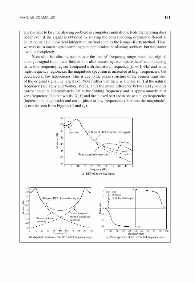
JWBK207-06 JWBK207-Shin January 26, 2008 18:29 Char Count= 0
MATLAB EXAMPLES 181
always have to face the aliasing problem in computer simulations. Note that aliasing doesoccur even if the signal is obtained by solving the corresponding ordinary differentialequation using a numerical integration method such as the Runge–Kutta method. Thus,we may use a much higher sampling rate to minimize the aliasing problem, but we cannotavoid it completely.
Note also that aliasing occurs over the ‘entire’ frequency range, since the originalanalogue signal is not band-limited. It is also interesting to compare the effect of aliasingin the low-frequency region (compared with the natural frequency, fn = 10 Hz) and in thehigh-frequency region, i.e. the magnitude spectrum is increased at high frequencies, butdecreased at low frequencies. This is due to the phase structure of the Fourier transformof the original signal, i.e. arg X ( f ). Note further that there is a phase shift at the naturalfrequency (see Fahy and Walker, 1998). Thus the phase difference betweenX ( f )and itsmirror image is approximately 2π at the folding frequency and is approximately π atzero frequency. In other words, X ( f ) and the aliased part are in phase at high frequencies(increase the magnitude) and out of phase at low frequencies (decrease the magnitude),as can be seen from Figures (f) and (g).
500-point DFT of noise-free signal
T
(e) DFT of noise-free signal
rue magnitude spectrum
0 5 10 15 20 25 30 35 40 45 50–55
–50
–45
–40
–35
–30
–25
–20
Frequency (Hz)
Modulu
s (d
B)
Aliasing
Aliasing
500-point DFT of noise-free signal
T
(f) Magnitude spectrum of the DFT in full frequency range
rue magnitude spectrum
0 10 20 30 40 50 60 70 80 90 100–65
–60
–55
–50
–45
–40
–35
–30
–25
–20
Frequency (Hz)
Modulu
s (d
B)
Mirror image of the true magnitude spectrum
0 10 20 30 40 50 60 70 80 90 100
–3
–2
–1
0
1
2
3
Frequency (Hz)
Phas
e (r
ad)
In phase
(g) Phase spectrum of the DFT in full frequency range
(with the aliased part)
Ou
tof
ph
ase
π
−π

JWBK207-06 JWBK207-Shin January 26, 2008 18:29 Char Count= 0
182 THE DISCRETE FOURIER TRANSFORM
Example 6.6: Circular (periodic) and linear convolutions using the DFT
Consider the following two finite sequences of length N = 5:
x(n) = [1 3 5 3 1] and h(n) = [9 7 5 3 1]
Perform the circular convolution and the linear convolution using the DFT.
Line MATLAB code Comments
1 clear all Define the sequences x(n) and h(n).2 x=[1 3 5 3 1]; h=[9 7 5 3 1];
3 X=fft(x); H=fft(h); Perform the DFT of each sequence. Take theinverse DFT of the product X(k) and H(k) toobtain the circular convolution result. Definethe variable for the x-axis.
4 yp=ifft(X.*H);5 np=0:4;
6 figure(1) Plot the sequences x and h, and the results ofcircular convolution. Note that the sequencesx and h are periodic in effect.
7 subplot(3,1,1); stem(np, x, 'd', 'fill')8 axis([-0.4 4.4 0 6])9 xlabel('\itn');
ylabel('\itx p\rm(\itn\rm)')10 subplot(3,1,2); stem(np, h, 'fill')11 axis([-0.4 4.4 0 10])12 xlabel('\itn');
ylabel('\ith p\rm(\itn\rm)')13 subplot(3,1,3); stem(np, yp, 'fill')14 axis([-0.4 4.4 0 90])15 xlabel('\itn');
ylabel('\ity p\rm(\itn\rm)')
16 Xz=fft([x zeros(1,length(h)-1)]); Perform the linear convolution using theDFT. Note that zeros are added appropriatelywhen calculating DFT coefficients.Also, note that the MATLAB function‘conv(x, h)’ will give the same result (in fact,this function uses the same algorithm).
17 Hz=fft([h zeros(1,length(x)-1)]);18 yz=ifft(Xz.*Hz);19 nz=0:8;
20 figure(2) Plot the zero-padded sequences, and theresults of linear convolution using the DFT.21 subplot(3,1,1);
stem(nz, [x 0 0 0 0], 'd', 'fill')22 axis([-0.4 8.4 0 6])23 xlabel('\itn');
ylabel('\itx\rm(\itn\rm)')24 subplot(3,1,2);
stem(nz, [h 0 0 0 0], 'fill')25 axis([-0.4 8.4 0 10])26 xlabel('\itn');
ylabel('\ith\rm(\itn\rm)')27 subplot(3,1,3); stem(nz, yz, 'fill')28 axis([-0.4 8.4 0 90])29 xlabel('\itn');
ylabel('\ity\rm(\itn\rm)')
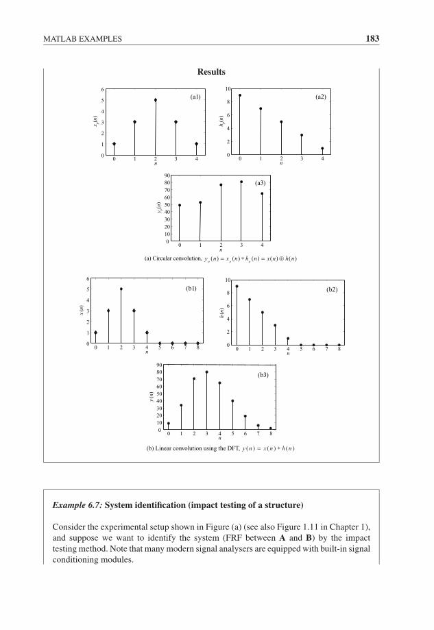
JWBK207-06 JWBK207-Shin January 26, 2008 18:29 Char Count= 0
MATLAB EXAMPLES 183
Results
n0 1 2 3 4
0
1
2
3
4
5
6x p(
n)(a1)
0 1 2 3 40
2
4
6
8
10
n
h p(n)
(a2)
y p(n)
0 1 2 3 40
10
20
30
40
50
60
70
80
90
n
(a3)
(a) Circular convolution, ( ) ( ) ( ) ( ) ( )p p p
y n x n h n x n h n= ∗ = ∗
y(n
)
0 1 2 3 4 5 6 7 80
10
20
30
40
50
60
70
80
90
n
(b3)
h(n
)
0 1 2 3 4 5 6 7 80
2
4
6
8
10
n
(b2)
x(n
)
0 1 2 3 4 5 6 7 80
1
2
3
4
5
6
n
(b1)
(b) Linear convolution using the DFT, ( ) ( ) ( )y n x n h n= ∗
Example 6.7: System identification (impact testing of a structure)
Consider the experimental setup shown in Figure (a) (see also Figure 1.11 in Chapter 1),and suppose we want to identify the system (FRF between A and B) by the impacttesting method. Note that many modern signal analysers are equipped with built-in signalconditioning modules.
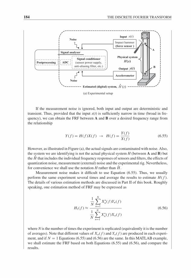
JWBK207-06 JWBK207-Shin January 26, 2008 18:29 Char Count= 0
184 THE DISCRETE FOURIER TRANSFORM
(a) Experimental setup
Impact hammer(force sensor )
Accelerometer
Input
Output
Physical system
A
B
( )x t
( )y t
( )H s
Signal Analyzer
Signal conditioner(sensor power supply,
anti-aliasing filter, etc.)
ADCPost-processing
ˆ
Noise
Noise
( )
( )y t
( )H s
Signal analyser
Signal conditioner(sensor power supply,
anti-aliasing filter, etc.)
ADCPostprocessing
Estimated (digital) system, H (z)
If the measurement noise is ignored, both input and output are deterministic andtransient. Thus, provided that the input x(t) is sufficiently narrow in time (broad in fre-quency), we can obtain the FRF between A and B over a desired frequency range fromthe relationship
Y ( f ) = H ( f )X ( f ) → H ( f ) = Y ( f )
X ( f )(6.55)
However, as illustrated in Figure (a), the actual signals are contaminated with noise. Also,the system we are identifying is not the actual physical system H (between A and B) butthe H that includes the individual frequency responses of sensors and filters, the effects ofquantization noise, measurement (external) noise and the experimental rig. Nevertheless,for convenience we shall use the notation H rather than H .
Measurement noise makes it difficult to use Equation (6.55). Thus, we usuallyperform the same experiment several times and average the results to estimate H ( f ).The details of various estimation methods are discussed in Part II of this book. Roughlyspeaking, one estimation method of FRF may be expressed as
H1( f ) ≈
1
N
N∑n=1
X∗n( f )Yn( f )
1
N
N∑n=1
X∗n( f )Xn( f )
(6.56)
where N is the number of times the experiment is replicated (equivalently it is the numberof averages). Note that different values of Xn( f ) and Yn( f ) are produced in each experi-ment, and if N = 1 Equations (6.55) and (6.56) are the same. In this MATLAB example,we shall estimate the FRF based on both Equations (6.55) and (6.56), and compare theresults.
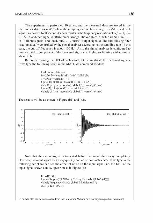
JWBK207-06 JWBK207-Shin January 26, 2008 18:29 Char Count= 0
MATLAB EXAMPLES 185
The experiment is performed 10 times, and the measured data are stored in thefile ‘impact data raw.mat’,1 where the sampling rate is chosen as fs = 256 Hz, and eachsignal is recorded for 8 seconds (which results in the frequency resolution of � f = 1/8 =0.125 Hz, and each signal is 2048 elements long). The variables in the file are ‘in1, in2, . . . ,in10’ (input signals) and ‘out1, out2, . . . , out10’ (output signals). The anti-aliasing filteris automatically controlled by the signal analyser according to the sampling rate (in thiscase, the cut-off frequency is about 100 Hz). Also, the signal analyser is configured toremove the d.c. component of the measured signal (i.e. high-pass filtering with cut-on atabout 5 Hz).
Before performing the DFT of each signal, let us investigate the measured signals.If we type the following script in the MATLAB command window:
load impact data rawfs=256; N=length(in1); f=fs*(0:N-1)/N;T=N/fs; t=0:1/fs:T-1/fs;figure(1); plot(t, in1); axis([-0.1 8 -1.5 2.5])xlabel('\itt\rm (seconds)'); ylabel('\itx\rm(\itt\rm)')figure(2); plot(t, out1); axis([-0.1 8 -4 4])xlabel('\itt\rm (seconds)'); ylabel('\ity\rm(\itt\rm)')
The results will be as shown in Figure (b1) and (b2).
0 1 2 3 4 5 6 7 8–1.5
–1
–0.5
0
0.5
1
1.5
2
2.5
t (seconds)
x(t)
(b1) Input signal
0 1 2 3 4 5 6 7 8–4
–3
–2
–1
0
1
2
3
4
t (seconds)
y(t)
(b2) Output signal
Note that the output signal is truncated before the signal dies away completely.However, the input signal dies away quickly and noise dominates later. If we type in thefollowing script we can see the effect of noise on the input signal, i.e. the DFT of theinput signal shows a noisy spectrum as in Figure (c):
In1=fft(in1);figure (3); plot(f(1:N/2+1), 20*log10(abs(In1(1:N/2+1))))xlabel('Frequency (Hz)'); ylabel('Modulus (dB)')axis([0 128 -70 30])
1 The data files can be downloaded from the Companion Website (www.wiley.com/go/shin hammond)
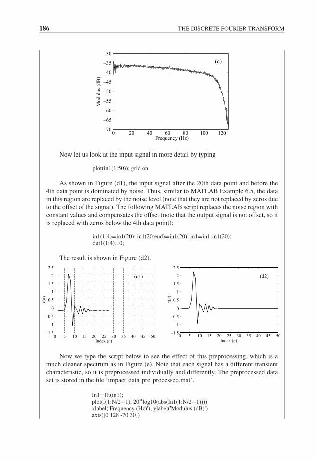
JWBK207-06 JWBK207-Shin January 26, 2008 18:29 Char Count= 0
186 THE DISCRETE FOURIER TRANSFORM
0 20 40 60 80 100 120–70
–65
–60
–55
–50
–45
–40
–35
–30
Frequency (Hz)
Modulu
s (d
B)
(c)
Now let us look at the input signal in more detail by typing
plot(in1(1:50)); grid on
As shown in Figure (d1), the input signal after the 20th data point and before the4th data point is dominated by noise. Thus, similar to MATLAB Example 6.5, the datain this region are replaced by the noise level (note that they are not replaced by zeros dueto the offset of the signal). The following MATLAB script replaces the noise region withconstant values and compensates the offset (note that the output signal is not offset, so itis replaced with zeros below the 4th data point):
in1(1:4)=in1(20); in1(20:end)=in1(20); in1=in1-in1(20);out1(1:4)=0;
The result is shown in Figure (d2).
Index (n)0 5 10 15 20 25 30 35 40 45 50
–1.5
–1
–0.5
0
0.5
1
1.5
2
2.5
x(n)
(d1)
0 5 10 15 20 25 30 35 40 45 50–1.5
–1
–0.5
0
0.5
1
1.5
2
2.5
Index (n)
x(n)
(d2)
Now we type the script below to see the effect of this preprocessing, which is amuch cleaner spectrum as in Figure (e). Note that each signal has a different transientcharacteristic, so it is preprocessed individually and differently. The preprocessed dataset is stored in the file ‘impact data pre processed.mat’.
In1=fft(in1);plot(f(1:N/2+1), 20*log10(abs(In1(1:N/2+1))))xlabel('Frequency (Hz)'); ylabel('Modulus (dB)')axis([0 128 -70 30])
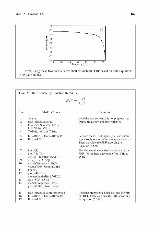
JWBK207-06 JWBK207-Shin January 26, 2008 18:29 Char Count= 0
MATLAB EXAMPLES 187
0 20 40 60 80 100 120–70
–65
–60
–55
–50
–45
–40
–35
–30
Frequency (Hz)
Modulu
s (d
B)
(e)
Now, using these two data sets, we shall estimate the FRF based on both Equations(6.55) and (6.56).
Case A: FRF estimate by Equation (6.55), i.e.
H ( f ) = Y ( f )
X ( f )
Line MATLAB code Comments
1 clear all Load the data set which is not preprocessed.Define frequency and time variables.2 load impact data raw
3 fs = 256; N = length(in1);f=fs*(0:N-1)/N;
4 T=N/fs; t=0:1/fs:T-1/fs;
5 In1=fft(in1); Out1=fft(out1); Perform the DFT of input signal and outputsignal (only one set of input–output records).Then, calculate the FRF according toEquation (6.55).
6 H=Out1./In1;
7 figure(1) Plot the magnitude and phase spectra of theFRF (for the frequency range from 5 Hz to95 Hz).
8 plot(f(41:761),20*log10(abs(H(41:761))))
9 axis([5 95 -30 50])10 xlabel('Frequency (Hz)');
ylabel('FRF (Modulus, dB)')11 figure(2)12 plot(f(41:761),
unwrap(angle(H(41:761))))13 axis([5 95 -3.5 3.5])14 xlabel('Frequency (Hz)');
ylabel('FRF (Phase, rad)')
15 load impact data pre processed Load the preprocessed data set, and performthe DFT. Then, calculate the FRF accordingto Equation (6.55).
16 In1=fft(in1); Out1=fft(out1);17 H=Out1./In1;
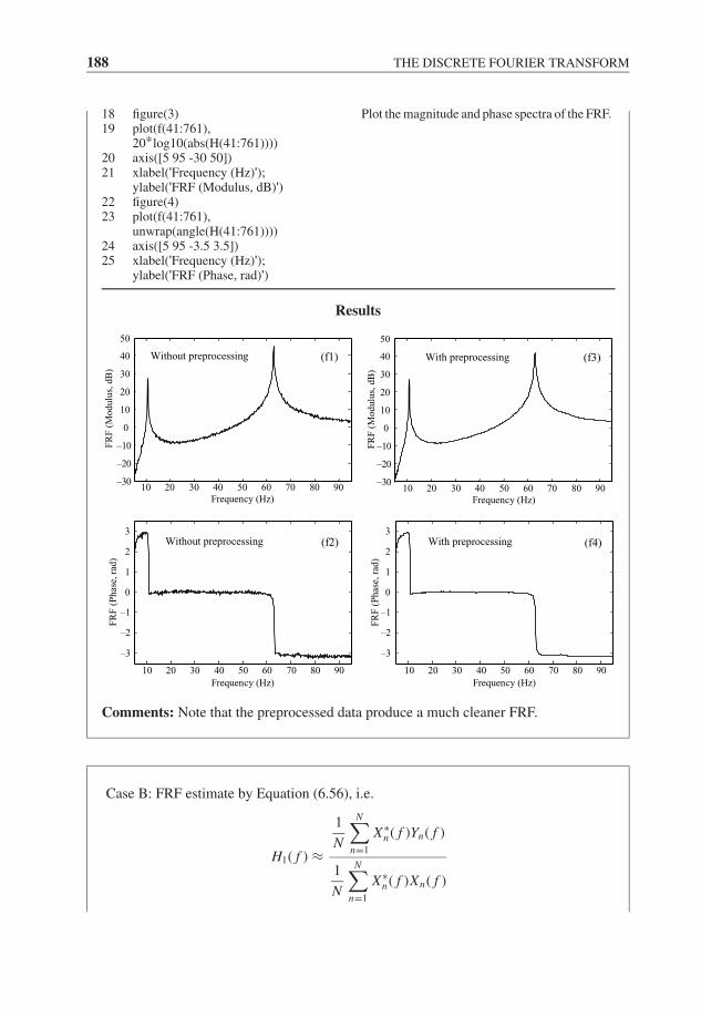
JWBK207-06 JWBK207-Shin January 26, 2008 18:29 Char Count= 0
188 THE DISCRETE FOURIER TRANSFORM
18 figure(3) Plot the magnitude and phase spectra of the FRF.19 plot(f(41:761),
20*log10(abs(H(41:761))))20 axis([5 95 -30 50])21 xlabel('Frequency (Hz)');
ylabel('FRF (Modulus, dB)')22 figure(4)23 plot(f(41:761),
unwrap(angle(H(41:761))))24 axis([5 95 -3.5 3.5])25 xlabel('Frequency (Hz)');
ylabel('FRF (Phase, rad)')
Results
10 20 30 40 50 60 70 80 90
–3
–2
–1
0
1
2
3
Frequency (Hz)
FR
F (
Ph
ase,
rad
)
(f4)With preprocessing
10 20 30 40 50 60 70 80 90–30
–20
–10
0
10
20
30
40
50
Frequency (Hz)
FR
F (
Mo
du
lus,
dB
)
(f3)With preprocessing
10 20 30 40 50 60 70 80 90–30
–20
–10
0
10
20
30
40
50
Frequency (Hz)
FR
F (
Mo
du
lus,
dB
)
(f1)Without preprocessing
10 20 30 40 50 60 70 80 90
–3
–2
–1
0
1
2
3
Frequency (Hz)
FR
F (
Ph
ase,
rad
)
(f2)Without preprocessing
Comments: Note that the preprocessed data produce a much cleaner FRF.
Case B: FRF estimate by Equation (6.56), i.e.
H1( f ) ≈
1
N
N∑n=1
X∗n( f )Yn( f )
1
N
N∑n=1
X∗n( f )Xn( f )

JWBK207-06 JWBK207-Shin January 26, 2008 18:29 Char Count= 0
MATLAB EXAMPLES 189
Line MATLAB code Comments
1 clear all Load the data set which is not preprocessed(Line 2).Later, comment out this line (with %), anduncomment Line 3 to load the preprocesseddata set.Define frequency and time variables.
2 load impact data raw3 % load impact data pre processed4 fs = 256; N = length(in1);
f=fs*(0:N-1)/N;5 T=N/fs; t=0:1/fs:T-1/fs;
6 Navg=10;% Navg=3 for preprocessed data set
Define the number of averages N = 10 (seeEquation (6.56)). Later, use N = 3 for thepreprocessed data set.
7 for n=1:Navg This ‘for’ loop produces variables: In1,In2, . . . , In10; Out1, Out2, . . . , Out10; Sxx1,Sxx2, . . . , Sxx10; Sxy1, Sxy2, . . . , Sxy10.They are the DFTs of input and output signals,and the elements of the numerator anddenominator of Equation (6.56), such that, forexample, In1 = X1, Out1 = Y1,Sxx1 = X∗
1 X1 and Sxy1 = X∗1Y1.
For more details of the ‘eval’ function see theMATLAB help window.
8 In = ['In', int2str(n), '= fft(in',int2str(n), ');'];
9 eval(In);10 Out = ['Out', int2str(n), '= fft(out',
int2str(n), ');'];11 eval(Out);12 Sxx = ['Sxx', int2str(n), '=conj(In',
int2str(n), ')' '.*In', int2str(n), ';'];13 eval(Sxx);14 Sxy = ['Sxy', int2str(n), '= conj(In',
int2str(n), ')' '.*Out', int2str(n), ';'];15 eval(Sxy);16 end
17 Sxx=[]; Sxy=[]; Define empty matrices which will be used inthe ‘for’ loop.The ‘for’ loop produces two matrices Sxx andSxy, where the nth row of the matrices isX∗
n Xn and X∗nYn , respectively.
18 for n=1:Navg19 tmp1= ['Sxx', int2str(n), ';'];20 Sxx=[Sxx; eval(tmp1)];21 tmp2= ['Sxy', int2str(n), ';'];22 Sxy=[Sxy; eval(tmp2)];23 end
24 Sxx=mean(Sxx); Sxy=mean(Sxy); First calculate the numerator and denominatorof Equation (6.56), and then H1 is obtained.25 H1=Sxy./Sxx;
26 figure(1) Plot the magnitude and phase spectra of theFRF.Run this MATLAB program again using thepreprocessed data set, and compare the results.
27 plot(f(41:761),20*log10(abs(H(41:761))))
28 axis([5 95 -30 50])29 xlabel('Frequency (Hz)');
ylabel('FRF (Modulus, dB)')30 figure(2)31 plot(f(41:761),
unwrap(angle(H1(41:761))))32 axis([5 95 -3.5 3.5])33 xlabel('Frequency (Hz)');
ylabel('FRF (Phase, rad)')
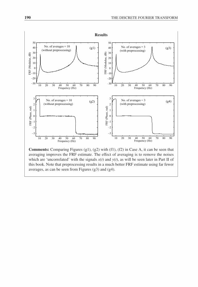
JWBK207-06 JWBK207-Shin January 26, 2008 18:29 Char Count= 0
190 THE DISCRETE FOURIER TRANSFORM
Results
No. of averages = 10 (without preprocessing)
10 20 30 40 50 60 70 80 90–30
–20
–10
0
10
20
30
40
50
Frequency (Hz)
FR
F (
Mo
du
lus,
dB
)
(g1)
10 20 30 40 50 60 70 80 90
–3
–2
–1
0
1
2
3
Frequency (Hz)
FR
F (
Ph
ase,
rad
)
(g2)No. of averages = 10 (without preprocessing)
10 20 30 40 50 60 70 80 90–30
–20
–10
0
10
20
30
40
50
Frequency (Hz)
FR
F (
Mo
du
lus,
dB
)
(g3)No. of averages = 3 (with preprocessing)
10 20 30 40 50 60 70 80 90
–3
–2
–1
0
1
2
3
Frequency (Hz)
FR
F (
Ph
ase,
rad
)
(g4)No. of averages = 3 (with preprocessing)
Comments: Comparing Figures (g1), (g2) with (f1), (f2) in Case A, it can be seen thataveraging improves the FRF estimate. The effect of averaging is to remove the noiseswhich are ‘uncorrelated’ with the signals x(t) and y(t), as will be seen later in Part II ofthis book. Note that preprocessing results in a much better FRF estimate using far feweraverages, as can be seen from Figures (g3) and (g4).

JWBK207-07 JWBK207-Shin January 26, 2008 17:21 Char Count= 0
Part IIIntroduction to Random Processes
191

JWBK207-07 JWBK207-Shin January 26, 2008 17:21 Char Count= 0
192
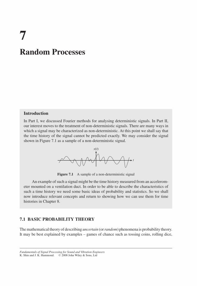
JWBK207-07 JWBK207-Shin January 26, 2008 17:21 Char Count= 0
7Random Processes
Introduction
In Part I, we discussed Fourier methods for analysing deterministic signals. In Part II,our interest moves to the treatment of non-deterministic signals. There are many ways inwhich a signal may be characterized as non-deterministic. At this point we shall say thatthe time history of the signal cannot be predicted exactly. We may consider the signalshown in Figure 7.1 as a sample of a non-deterministic signal.
x(t)
t
Figure 7.1 A sample of a non-deterministic signal
An example of such a signal might be the time history measured from an accelerom-eter mounted on a ventilation duct. In order to be able to describe the characteristics ofsuch a time history we need some basic ideas of probability and statistics. So we shallnow introduce relevant concepts and return to showing how we can use them for timehistories in Chapter 8.
7.1 BASIC PROBABILITY THEORY
The mathematical theory of describing uncertain (or random) phenomena is probability theory.It may be best explained by examples – games of chance such as tossing coins, rolling dice,
Fundamentals of Signal Processing for Sound and Vibration EngineersK. Shin and J. K. Hammond. C© 2008 John Wiley & Sons, Ltd
193
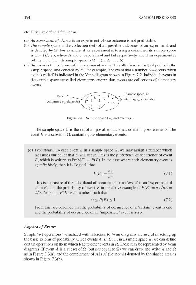
JWBK207-07 JWBK207-Shin January 26, 2008 17:21 Char Count= 0
194 RANDOM PROCESSES
etc. First, we define a few terms:
(a) An experiment of chance is an experiment whose outcome is not predictable.(b) The sample space is the collection (set) of all possible outcomes of an experiment, and
is denoted by �. For example, if an experiment is tossing a coin, then its sample spaceis � = (H, T ), where H and T denote head and tail respectively, and if an experiment isrolling a die, then its sample space is � = (1, 2, . . . , 6).
(c) An event is the outcome of an experiment and is the collection (subset) of points in thesample space, and denoted by E . For example, ‘the event that a number ≤ 4 occurs whena die is rolled’ is indicated in the Venn diagram shown in Figure 7.2. Individual events inthe sample space are called elementary events, thus events are collections of elementaryevents.
Sample space,
elements)(containing nΩ
ΩEvent, E
elements)(containing nE
E Ω1
35 6
2
4
Figure 7.2 Sample space (�) and event (E)
The sample space � is the set of all possible outcomes, containing n� elements. Theevent E is a subset of �, containing nE elementary events.
(d) Probability: To each event E in a sample space �, we may assign a number whichmeasures our belief that E will occur. This is the probability of occurrence of eventE , which is written as Prob[E] = P(E). In the case where each elementary event isequally likely, then it is ‘logical’ that
P(E) = nE
n�
(7.1)
This is a measure of the ‘likelihood of occurrence’ of an ‘event’ in an ‘experiment ofchance’, and the probability of event E in the above example is P(E) = nE
/n� =
2/
3. Note that P(E) is a ‘number’ such that
0 ≤ P(E) ≤ 1 (7.2)
From this, we conclude that the probability of occurrence of a ‘certain’ event is oneand the probability of occurrence of an ‘impossible’ event is zero.
Algebra of Events
Simple ‘set operations’ visualized with reference to Venn diagrams are useful in setting upthe basic axioms of probability. Given events A, B, C , . . . in a sample space �, we can definecertain operations on them which lead to other events in �. These may be represented by Venndiagrams. If event A is a subset of � (but not equal to �) we can draw and write A and �
as in Figure 7.3(a), and the complement of A is A′ (i.e. not A) denoted by the shaded area asshown in Figure 7.3(b).
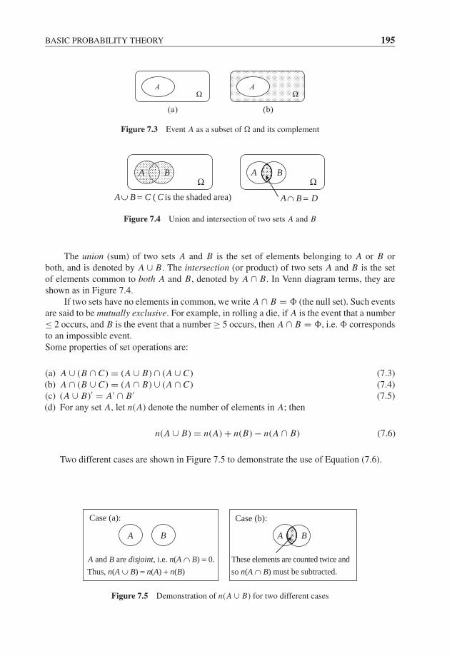
JWBK207-07 JWBK207-Shin January 26, 2008 17:21 Char Count= 0
BASIC PROBABILITY THEORY 195
(a) (b)
AΩΩ
A
Figure 7.3 Event A as a subset of � and its complement
AΩ
is the shaded area) ( CCBA =∪
BΩ
BA
DBA =∩
Figure 7.4 Union and intersection of two sets A and B
The union (sum) of two sets A and B is the set of elements belonging to A or B orboth, and is denoted by A ∪ B. The intersection (or product) of two sets A and B is the setof elements common to both A and B, denoted by A ∩ B. In Venn diagram terms, they areshown as in Figure 7.4.
If two sets have no elements in common, we write A ∩ B = � (the null set). Such eventsare said to be mutually exclusive. For example, in rolling a die, if A is the event that a number≤ 2 occurs, and B is the event that a number ≥ 5 occurs, then A ∩ B = �, i.e. � correspondsto an impossible event.Some properties of set operations are:
(a) A ∪ (B ∩ C) = (A ∪ B) ∩ (A ∪ C) (7.3)(b) A ∩ (B ∪ C) = (A ∩ B) ∪ (A ∩ C) (7.4)(c) (A ∪ B)′ = A′ ∩ B ′ (7.5)(d) For any set A, let n(A) denote the number of elements in A; then
n(A ∪ B) = n(A) + n(B) − n(A ∩ B) (7.6)
Two different cases are shown in Figure 7.5 to demonstrate the use of Equation (7.6).
Case (a): Case (b):
BABA
Thus, n(A ∪ B) = n(A) + n(B)
A and B are disjoint, i.e. n(A ∩ B) = 0. These elements are counted twice and
so n(A ∩ B) must be subtracted.
Figure 7.5 Demonstration of n(A ∪ B) for two different cases

JWBK207-07 JWBK207-Shin January 26, 2008 17:21 Char Count= 0
196 RANDOM PROCESSES
Algebra of Probabilities
The above intuitive ideas are formalized into the axioms of probability as follows. Toeach event Ei (in a sample space �), we assign a number called the probability of Ei
(denoted P(Ei )) such that
(a) 0 ≤ P(Ei ) ≤ 1 (7.7)(b) If Ei and E j are mutually exclusive, then
P(Ei ∪ E j ) = P(Ei ) + P(E j ) (7.8)
(c) If⋃
Ei = �, then
P( ⋃
Ei) = 1 (7.9)
(d) P(�) = 0 (7.10)(e) For any events E1, E2, not necessarily mutually exclusive,
P(E1 ∪ E2) = P(E1) + P(E2) − P(E1 ∩ E2) (7.11)
Equally Likely Events
If n events, E1, E2, . . . ,En , are judged to be equally likely, then
P(Ei ) = 1
n(7.12)
As an example of this, throw two dice and record the number on each face. What isthe probability of the event that the total score is 5? The answer is P(E5) = nE5
/n� =4/36 = 1/9.
Joint Probability
The probability of occurrence of events A and B jointly is called a joint probability and isdenoted P(A ∩ B) or P(A, B). With reference to Figure 7.6, this is the occurrence of theshaded area, i.e.
P(A ∩ B) = n A∩B
n�
(7.13)
AΩ
B
Figure 7.6 The intersection of two sets A and B in a sample space �
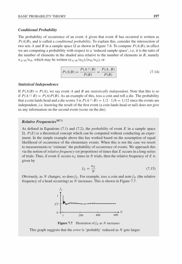
JWBK207-07 JWBK207-Shin January 26, 2008 17:21 Char Count= 0
BASIC PROBABILITY THEORY 197
Conditional Probability
The probability of occurrence of an event A given that event B has occurred is written asP(A|B), and is called a conditional probability. To explain this, consider the intersection oftwo sets A and B in a sample space � as shown in Figure 7.6. To compute P(A|B), in effectwe are computing a probability with respect to a ‘reduced sample space’, i.e. it is the ratio ofthe number of elements in the shaded area relative to the number of elements in B, namelyn A∩B/nB , which may be written (n A∩B/n�)/(nB/n�), or
P(A|B) = P(A ∩ B)
P(B)= P(A, B)
P(B)(7.14)
Statistical Independence
If P(A|B) = P(A), we say event A and B are statistically independent. Note that this is soif P(A ∩ B) = P(A)P(B). As an example of this, toss a coin and roll a die. The probabilitythat a coin lands head and a die scores 3 is P(A ∩ B) = 1/2 · 1/6 = 1/12 since the events areindependent, i.e. knowing the result of the first event (a coin lands head or tail) does not giveus any information on the second event (score on the die).
Relative FrequenciesM7.1
As defined in Equations (7.1) and (7.2), the probability of event E in a sample space�, P(E) is a theoretical concept which can be computed without conducting an exper-iment. In the simple example above this has worked based on the assumption of equallikelihood of occurrence of the elementary events. When this is not the case we resortto measurements to ‘estimate’ the probability of occurrence of events. We approach thisvia the notion of relative frequency (or proportion) of times that E occurs in a long seriesof trials. Thus, if event E occurs nE times in N trials, then the relative frequency of E isgiven by
fE = nE
N(7.15)
Obviously, as N changes, so does fE . For example, toss a coin and note fH (the relativefrequency of a head occurring) as N increases. This is shown in Figure 7.7.
1 2
1
0
Hf
1 200 400 600N
Figure 7.7 Illustration of fH as N increases
This graph suggests that the error is ‘probably’ reduced as N gets larger.
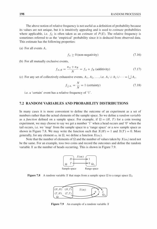
JWBK207-07 JWBK207-Shin January 26, 2008 17:21 Char Count= 0
198 RANDOM PROCESSES
The above notion of relative frequency is not useful as a definition of probability becauseits values are not unique, but it is intuitively appealing and is used to estimate probabilitieswhere applicable, i.e. fE is often taken as an estimate of P(E). The relative frequency issometimes referred to as the ‘empirical’ probability since it is deduced from observed data.This estimate has the following properties:
(a) For all events A,
f A ≥ 0 (non-negativity) (7.16)
(b) For all mutually exclusive events,
f A∪B = n A + nB
N= f A + fB (additivity) (7.17)
(c) For any set of collectively exhaustive events, A1, A2, . . . , i.e. A1 ∪ A2 ∪ · · · = ⋃Ai ,
f⋃ Ai = N
N= 1 (certainty) (7.18)
i.e. a ‘certain’ event has a relative frequency of ‘1’.
7.2 RANDOM VARIABLES AND PROBABILITY DISTRIBUTIONS
In many cases it is more convenient to define the outcome of an experiment as a set ofnumbers rather than the actual elements of the sample space. So we define a random variableas a function defined on a sample space. For example, if � = (H, T ) for a coin tossingexperiment, we may choose to say we get a number ‘1’ when a head occurs and ‘0’ when thetail occurs, i.e. we ‘map’ from the sample space to a ‘range space’ or a new sample space asshown in Figure 7.8. We may write the function such that X (H ) = 1 and X (T ) = 0. Moregenerally, for any element ωi in �, we define a function X (ωi ).
Note that the number of elements of � and the number of values taken by X (ωi ) need notbe the same. For an example, toss two coins and record the outcomes and define the randomvariable X as the number of heads occurring. This is shown in Figure 7.9.
Sample space
Ω
( )iX ω
Range space
1
0
H
TXΩ
Figure 7.8 A random variable X that maps from a sample space � to a range space �X
( )iX ω( , )H H0 1 2
XΩΩ
( , )H T
( , )T H ( , )T T
Figure 7.9 An example of a random variable X
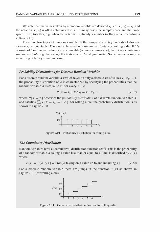
JWBK207-07 JWBK207-Shin January 26, 2008 17:21 Char Count= 0
RANDOM VARIABLES AND PROBABILITY DISTRIBUTIONS 199
We note that the values taken by a random variable are denoted xi , i.e. X (ωi ) = xi , andthe notation X (ωi ) is often abbreviated to X . In many cases the sample space and the rangespace ‘fuse’ together, e.g. when the outcome is already a number (rolling a die, recording avoltage, etc.).
There are two types of random variable. If the sample space �X consists of discreteelements, i.e. countable, X is said to be a discrete random variable, e.g. rolling a die. If �X
consists of ‘continuous’ values, i.e. uncountable (or non-denumerable), then X is a continuousrandom variable, e.g. the voltage fluctuation on an ‘analogue’ meter. Some processes may bemixed, e.g. a binary signal in noise.
Probability Distributions for Discrete Random Variables
For a discrete random variable X (which takes on only a discrete set of values x1, x2, . . . ),the probability distribution of X is characterized by specifying the probabilities that therandom variable X is equal to xi , for every xi , i.e.
P [X = xi ] for xi = x1, x2, . . . (7.19)
where P[X = xi ] describes the probability distribution of a discrete random variable Xand satisfies
∑i P[X = xi ] = 1, e.g. for rolling a die, the probability distribution is as
shown in Figure 7.10.
iP[X x ]=
1 2 3 4 5 6
1 6
ix
Figure 7.10 Probability distribution for rolling a die
The Cumulative Distribution
Random variables have a (cumulative) distribution function (cdf). This is the probabilityof a random variable X taking a value less than or equal to x . This is described by F(x)where
F(x) = P[X ≤ x] = Prob[X taking on a value up to and including x] (7.20)
For a discrete random variable there are jumps in the function F(x) as shown inFigure 7.11 (for rolling a die).
F(x)
x1 2 3 4 5 6
1 6
1 2
5 61
Figure 7.11 Cumulative distribution function for rolling a die
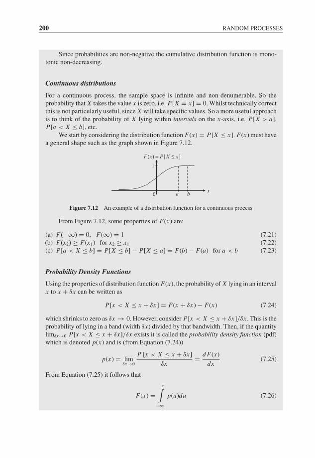
JWBK207-07 JWBK207-Shin January 26, 2008 17:21 Char Count= 0
200 RANDOM PROCESSES
Since probabilities are non-negative the cumulative distribution function is mono-tonic non-decreasing.
Continuous distributions
For a continuous process, the sample space is infinite and non-denumerable. So theprobability that X takes the value x is zero, i.e. P[X = x] = 0. Whilst technically correctthis is not particularly useful, since X will take specific values. So a more useful approachis to think of the probability of X lying within intervals on the x-axis, i.e. P[X > a],P[a < X ≤ b], etc.
We start by considering the distribution function F(x) = P[X ≤ x]. F(x) must havea general shape such as the graph shown in Figure 7.12.
( )F x P X x= ≤
1
0 a bx
[ ]
Figure 7.12 An example of a distribution function for a continuous process
From Figure 7.12, some properties of F(x) are:
(a) F(−∞) = 0, F(∞) = 1 (7.21)(b) F(x2) ≥ F(x1) for x2 ≥ x1 (7.22)(c) P[a < X ≤ b] = P[X ≤ b] − P[X ≤ a] = F(b) − F(a) for a < b (7.23)
Probability Density Functions
Using the properties of distribution function F(x), the probability of X lying in an intervalx to x + δx can be written as
P[x < X ≤ x + δx] = F(x + δx) − F(x) (7.24)
which shrinks to zero as δx → 0. However, consider P[x < X ≤ x + δx]/δx . This is theprobability of lying in a band (width δx) divided by that bandwidth. Then, if the quantitylimδx→0 P[x < X ≤ x + δx]/δx exists it is called the probability density function (pdf)which is denoted p(x) and is (from Equation (7.24))
p(x) = limδx→0
P [x < X ≤ x + δx]
δx= d F(x)
dx(7.25)
From Equation (7.25) it follows that
F(x) =x∫
−∞p(u)du (7.26)
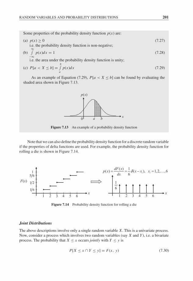
JWBK207-07 JWBK207-Shin January 26, 2008 17:21 Char Count= 0
RANDOM VARIABLES AND PROBABILITY DISTRIBUTIONS 201
Some properties of the probability density function p(x) are:
(a) p(x) ≥ 0 (7.27)i.e. the probability density function is non-negative;
(b)∞∫
−∞p(x)dx = 1 (7.28)
i.e. the area under the probability density function is unity;
(c) P[a < X ≤ b] =b∫
ap(x)dx (7.29)
As an example of Equation (7.29), P[a < X ≤ b] can be found by evaluating theshaded area shown in Figure 7.13.
( )p x
0 a b x
Figure 7.13 An example of a probability density function
Note that we can also define the probability density function for a discrete random variableif the properties of delta functions are used. For example, the probability density function forrolling a die is shown in Figure 7.14.
F(x)
1 2 3 4 5 6
1 6
1 2
5 61
x
1
6
( ) 1( ) ( ), 1, 2, ,6
6i i
dF xp x x x x
dxδ= = − =
1 2 3 4 5 6x
Figure 7.14 Probability density function for rolling a die
Joint Distributions
The above descriptions involve only a single random variable X . This is a univariate process.Now, consider a process which involves two random variables (say X and Y ), i.e. a bivariateprocess. The probability that X ≤ x occurs jointly with Y ≤ y is
P[X ≤ x ∩ Y ≤ y] = F(x, y) (7.30)
JWBK207-07 JWBK207-Shin January 26, 2008 17:21 Char Count= 0
202 RANDOM PROCESSES
Note thatF(−∞, y) = F(x, −∞) = 0, F(∞, ∞) = 1, F(x, ∞) = F(x) and F(∞, y) =F(y). Similar to the univariate case the ‘joint probability density function’ is defined as
p(x, y) = limδx→0δy→0
P[x < X ≤ x + δx ∩ y < Y ≤ y + δy]
δxδy= ∂2 F(x, y)
∂x∂y(7.31)
and
F(x, y) =x∫
−∞
y∫−∞
p(u, v)dvdu (7.32)
Note that
∞∫−∞
∞∫−∞
p(x, y)dydx = 1 and
x∫−∞
∞∫−∞
p(u, v)dvdu = F(x)
hence
p(x) =∞∫
−∞p(x, y)dy (7.33)
This is called a ‘marginal’ probability density function.These ideas may be extended to n random variables, X1, X2, . . . , Xn , i.e. we may define
p(x1, x2, . . . , xn). We shall only consider univariate and bivariate processes in this book.
7.3 EXPECTATIONS OF FUNCTIONS OF A RANDOM VARIABLE
So far, we have used probability distributions to describe the properties of random vari-ables. However, rather than using probability distributions, we often use averages. Thisintroduces the concept of the expectation of a process.
Consider a discrete random variable X which can assume any values x1, x2, . . . withprobabilities p1, p2, . . . . If xi occurs ni times in N trials of an experiment, then theaverage value of X is
x = 1
N
∑i
ni xi (7.34)
where x is called the sample mean. Since ni/N = fi (the empirical probability of oc-currence of xi ), Equation (7.34) can be written as x = ∑
i xi fi . As N → ∞, the empir-ical probability approaches the theoretical probability. So the expression for x becomes∑
i xi pi and this defines the theoretical mean value of X .For a continuous process, the probability pi may be replaced by the probability den-
sity multiplied by the bandwidth, i.e. pi → p(xi )δxi . So∑
i xi pi becomes∑
i xi p(xi )δxi
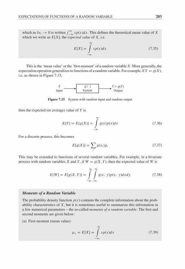
JWBK207-07 JWBK207-Shin January 26, 2008 17:21 Char Count= 0
EXPECTATIONS OF FUNCTIONS OF A RANDOM VARIABLE 203
which as δxi → 0 is written∫ ∞−∞ xp(x)dx . This defines the theoretical mean value of X
which we write as E[X ], the expected value of X , i.e.
E[X ] =∞∫
−∞xp(x)dx (7.35)
This is the ‘mean value’ or the ‘first moment’ of a random variable X . More generally, theexpectation operation generalizes to functions of a random variable. For example, if Y = g(X ),i.e. as shown in Figure 7.15,
Output
g(X )Y =)(System
gInput
X
Figure 7.15 System with random input and random output
then the expected (or average) value of Y is
E[Y ] = E[g(X )] =∞∫
−∞g(x)p(x)dx (7.36)
For a discrete process, this becomes
E[g(X )] =∑
i
g(xi )pi (7.37)
This may be extended to functions of several random variables. For example, in a bivariateprocess with random variables X and Y , if W = g(X, Y ), then the expected value of W is
E[W ] = E[g(X, Y )] =∞∫
−∞
∞∫−∞
g(x, y)p(x, y)dxdy (7.38)
Moments of a Random Variable
The probability density function p(x) contains the complete information about the prob-ability characteristics of X , but it is sometimes useful to summarize this information ina few numerical parameters – the so-called moments of a random variable. The first andsecond moments are given below:
(a) First moment (mean value):
μx = E[X ] =∞∫
−∞xp(x)dx (7.39)
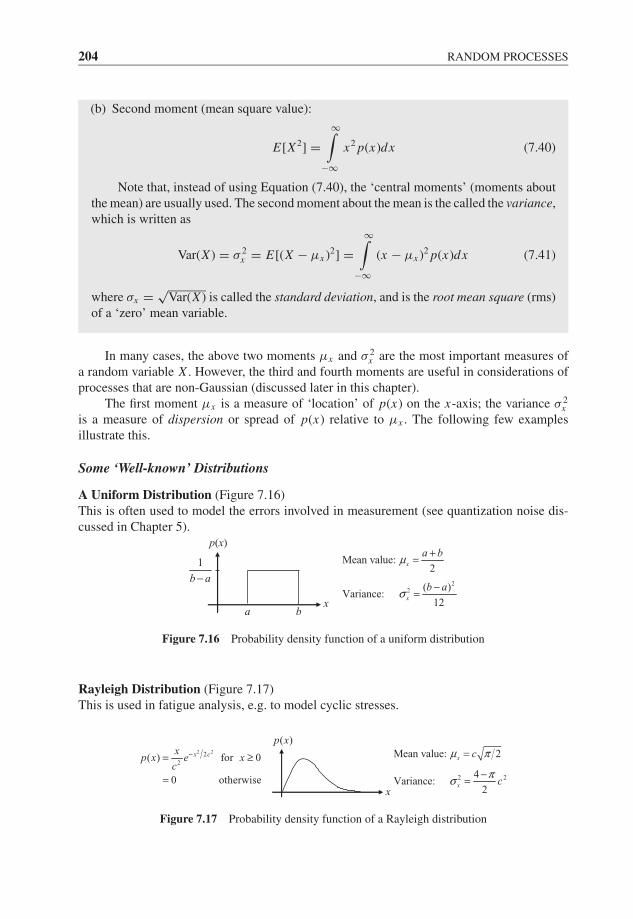
JWBK207-07 JWBK207-Shin January 26, 2008 17:21 Char Count= 0
204 RANDOM PROCESSES
(b) Second moment (mean square value):
E[X2] =∞∫
−∞x2 p(x)dx (7.40)
Note that, instead of using Equation (7.40), the ‘central moments’ (moments aboutthe mean) are usually used. The second moment about the mean is the called the variance,which is written as
Var(X ) = σ 2x = E[(X − μx )2] =
∞∫−∞
(x − μx )2 p(x)dx (7.41)
where σx = √Var(X ) is called the standard deviation, and is the root mean square (rms)
of a ‘zero’ mean variable.
In many cases, the above two moments μx and σ 2x are the most important measures of
a random variable X . However, the third and fourth moments are useful in considerations ofprocesses that are non-Gaussian (discussed later in this chapter).
The first moment μx is a measure of ‘location’ of p(x) on the x-axis; the variance σ 2x
is a measure of dispersion or spread of p(x) relative to μx . The following few examplesillustrate this.
Some ‘Well-known’ Distributions
A Uniform Distribution (Figure 7.16)This is often used to model the errors involved in measurement (see quantization noise dis-cussed in Chapter 5).
1
b a−2
2
Mean value:2
( )Variance:
12
x
x
a b
b a
μ
σ
+=
−=a b
p(x)
x
Figure 7.16 Probability density function of a uniform distribution
Rayleigh Distribution (Figure 7.17)This is used in fatigue analysis, e.g. to model cyclic stresses.
( )p x
x
2 2
Mean value: 2
4Variance:
2
x
x
c
c
μ π
πσ
=
−=
2 222
( ) for 0
0 otherwise
x cxp x e x
c−= ≥
=
Figure 7.17 Probability density function of a Rayleigh distribution
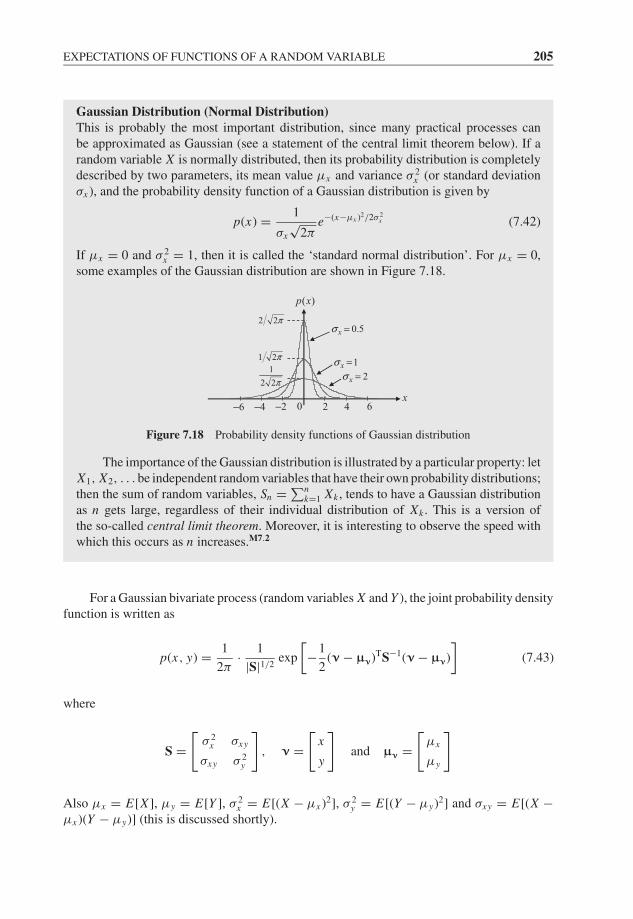
JWBK207-07 JWBK207-Shin January 26, 2008 17:21 Char Count= 0
EXPECTATIONS OF FUNCTIONS OF A RANDOM VARIABLE 205
Gaussian Distribution (Normal Distribution)This is probably the most important distribution, since many practical processes canbe approximated as Gaussian (see a statement of the central limit theorem below). If arandom variable X is normally distributed, then its probability distribution is completelydescribed by two parameters, its mean value μx and variance σ 2
x (or standard deviationσx ), and the probability density function of a Gaussian distribution is given by
p(x) = 1
σx
√2π
e−(x−μx )2/2σ 2x (7.42)
If μx = 0 and σ 2x = 1, then it is called the ‘standard normal distribution’. For μx = 0,
some examples of the Gaussian distribution are shown in Figure 7.18.
( )p x
0 2 4 6−2−4−6
1 2π1
2 2π
0.5xσ =
1xσ =2xσ =
2 2π
x
Figure 7.18 Probability density functions of Gaussian distribution
The importance of the Gaussian distribution is illustrated by a particular property: letX1, X2, . . . be independent random variables that have their own probability distributions;then the sum of random variables, Sn = ∑n
k=1 Xk , tends to have a Gaussian distributionas n gets large, regardless of their individual distribution of Xk . This is a version ofthe so-called central limit theorem. Moreover, it is interesting to observe the speed withwhich this occurs as n increases.M7.2
For a Gaussian bivariate process (random variables X and Y ), the joint probability densityfunction is written as
p(x, y) = 1
2π· 1
|S|1/2exp
[−1
2(ν − μν)TS−1(ν − μν)
](7.43)
where
S =[
σ 2x σxy
σxy σ 2y
], ν =
[x
y
]and μν =
[μx
μy
]
Also μx = E[X ], μy = E[Y ], σ 2x = E[(X − μx )2], σ 2
y = E[(Y − μy)2] and σxy = E[(X −μx )(Y − μy)] (this is discussed shortly).
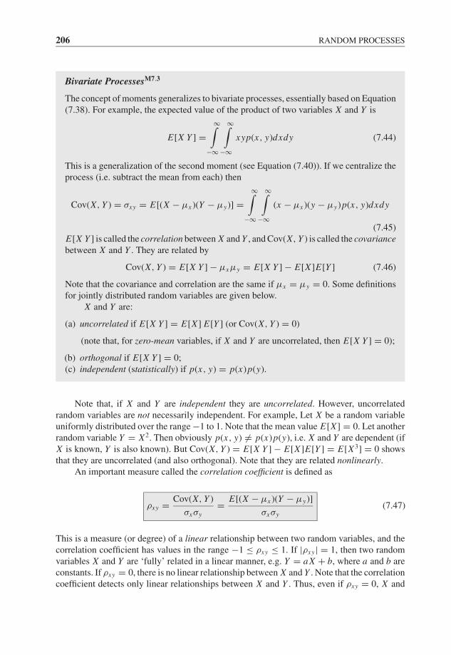
JWBK207-07 JWBK207-Shin January 26, 2008 17:21 Char Count= 0
206 RANDOM PROCESSES
Bivariate ProcessesM7.3
The concept of moments generalizes to bivariate processes, essentially based on Equation(7.38). For example, the expected value of the product of two variables X and Y is
E[X Y ] =∞∫
−∞
∞∫−∞
xyp(x, y)dxdy (7.44)
This is a generalization of the second moment (see Equation (7.40)). If we centralize theprocess (i.e. subtract the mean from each) then
Cov(X, Y ) = σxy = E[(X − μx )(Y − μy)] =∞∫
−∞
∞∫−∞
(x − μx )(y − μy)p(x, y)dxdy
(7.45)E[X Y ] is called the correlation between X and Y , and Cov(X, Y ) is called the covariancebetween X and Y . They are related by
Cov(X, Y ) = E[X Y ] − μxμy = E[X Y ] − E[X ]E[Y ] (7.46)
Note that the covariance and correlation are the same if μx = μy = 0. Some definitionsfor jointly distributed random variables are given below.
X and Y are:
(a) uncorrelated if E[X Y ] = E[X ] E[Y ] (or Cov(X, Y ) = 0)
(note that, for zero-mean variables, if X and Y are uncorrelated, then E[X Y ] = 0);
(b) orthogonal if E[X Y ] = 0;(c) independent (statistically) if p(x, y) = p(x)p(y).
Note that, if X and Y are independent they are uncorrelated. However, uncorrelatedrandom variables are not necessarily independent. For example, Let X be a random variableuniformly distributed over the range −1 to 1. Note that the mean value E[X ] = 0. Let anotherrandom variable Y = X2. Then obviously p(x, y) �= p(x)p(y), i.e. X and Y are dependent (ifX is known, Y is also known). But Cov(X, Y ) = E[X Y ] − E[X ]E[Y ] = E[X3] = 0 showsthat they are uncorrelated (and also orthogonal). Note that they are related nonlinearly.
An important measure called the correlation coefficient is defined as
ρxy = Cov(X, Y )
σxσy= E[(X − μx )(Y − μy)]
σxσy(7.47)
This is a measure (or degree) of a linear relationship between two random variables, and thecorrelation coefficient has values in the range −1 ≤ ρxy ≤ 1. If |ρxy | = 1, then two randomvariables X and Y are ‘fully’ related in a linear manner, e.g. Y = aX + b, where a and b areconstants. If ρxy = 0, there is no linear relationship between X and Y . Note that the correlationcoefficient detects only linear relationships between X and Y . Thus, even if ρxy = 0, X and
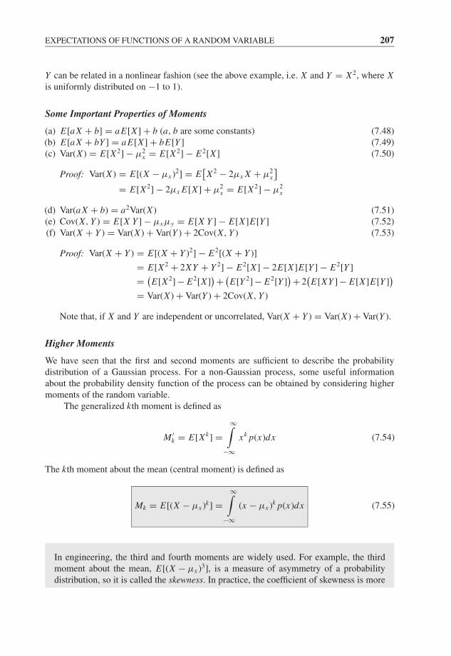
JWBK207-07 JWBK207-Shin January 26, 2008 17:21 Char Count= 0
EXPECTATIONS OF FUNCTIONS OF A RANDOM VARIABLE 207
Y can be related in a nonlinear fashion (see the above example, i.e. X and Y = X2, where Xis uniformly distributed on −1 to 1).
Some Important Properties of Moments
(a) E[aX + b] = aE[X ] + b (a, b are some constants) (7.48)(b) E[aX + bY ] = aE[X ] + bE[Y ] (7.49)(c) Var(X ) = E[X2] − μ2
x = E[X2] − E2[X ] (7.50)
Proof: Var(X ) = E[(X − μx )2] = E[X2 − 2μx X + μ2
x
]= E[X2] − 2μx E[X ] + μ2
x = E[X2] − μ2x
(d) Var(aX + b) = a2Var(X ) (7.51)(e) Cov(X, Y ) = E[X Y ] − μxμy = E[X Y ] − E[X ]E[Y ] (7.52)(f) Var(X + Y ) = Var(X ) + Var(Y ) + 2Cov(X, Y ) (7.53)
Proof: Var(X + Y ) = E[(X + Y )2] − E2[(X + Y )]
= E[X2 + 2XY + Y 2] − E2[X ] − 2E[X ]E[Y ] − E2[Y ]
= (E[X2] − E2[X ]
) + (E[Y 2] − E2[Y ]
) + 2(E[XY ] − E[X ]E[Y ]
)= Var(X ) + Var(Y ) + 2Cov(X, Y )
Note that, if X and Y are independent or uncorrelated, Var(X + Y ) = Var(X ) + Var(Y ).
Higher Moments
We have seen that the first and second moments are sufficient to describe the probabilitydistribution of a Gaussian process. For a non-Gaussian process, some useful informationabout the probability density function of the process can be obtained by considering highermoments of the random variable.
The generalized kth moment is defined as
M ′k = E[Xk] =
∞∫−∞
xk p(x)dx (7.54)
The kth moment about the mean (central moment) is defined as
Mk = E[(X − μx )k] =∞∫
−∞(x − μx )k p(x)dx (7.55)
In engineering, the third and fourth moments are widely used. For example, the thirdmoment about the mean, E[(X − μx )3], is a measure of asymmetry of a probabilitydistribution, so it is called the skewness. In practice, the coefficient of skewness is more
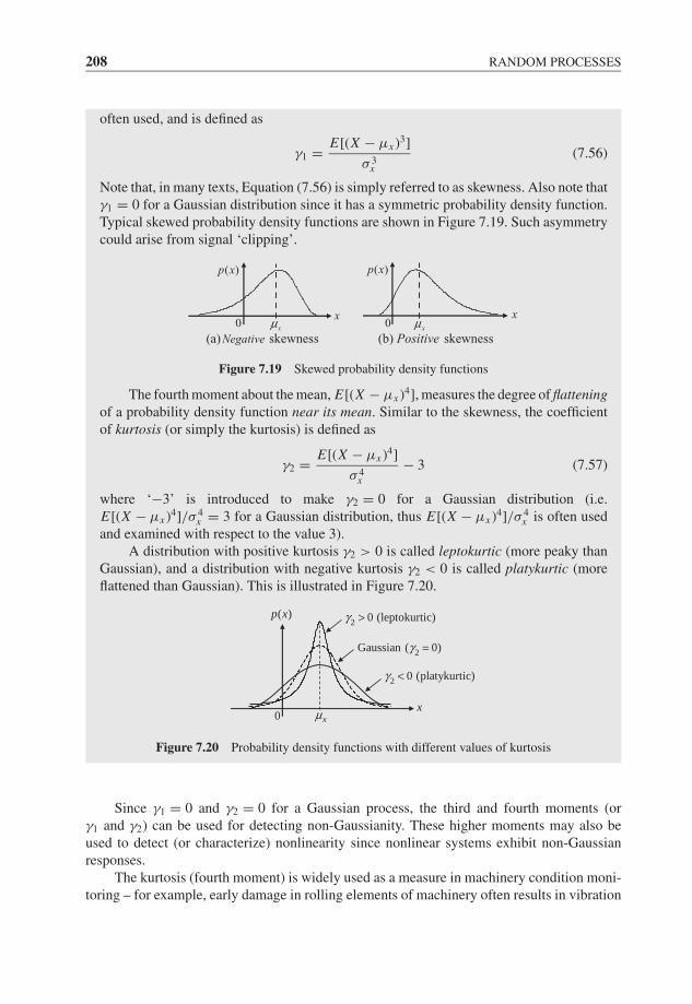
JWBK207-07 JWBK207-Shin January 26, 2008 17:21 Char Count= 0
208 RANDOM PROCESSES
often used, and is defined as
γ1 = E[(X − μx )3]
σ 3x
(7.56)
Note that, in many texts, Equation (7.56) is simply referred to as skewness. Also note thatγ1 = 0 for a Gaussian distribution since it has a symmetric probability density function.Typical skewed probability density functions are shown in Figure 7.19. Such asymmetrycould arise from signal ‘clipping’.
( )p x
x0 xμ
( )p x
x0 xμ
(a) skewnessNegative (b) skewnessPositive
Figure 7.19 Skewed probability density functions
The fourth moment about the mean, E[(X − μx )4], measures the degree of flatteningof a probability density function near its mean. Similar to the skewness, the coefficientof kurtosis (or simply the kurtosis) is defined as
γ2 = E[(X − μx )4]
σ 4x
− 3 (7.57)
where ‘−3’ is introduced to make γ2 = 0 for a Gaussian distribution (i.e.E[(X − μx )4]/σ 4
x = 3 for a Gaussian distribution, thus E[(X − μx )4]/σ 4x is often used
and examined with respect to the value 3).A distribution with positive kurtosis γ2 > 0 is called leptokurtic (more peaky than
Gaussian), and a distribution with negative kurtosis γ2 < 0 is called platykurtic (moreflattened than Gaussian). This is illustrated in Figure 7.20.
( )p x
xμ
2 0 (leptokurtic)γ >
2 0 (platykurtic)γ <
2Gaussian ( 0)γ =
x0
Figure 7.20 Probability density functions with different values of kurtosis
Since γ1 = 0 and γ2 = 0 for a Gaussian process, the third and fourth moments (orγ1 and γ2) can be used for detecting non-Gaussianity. These higher moments may also beused to detect (or characterize) nonlinearity since nonlinear systems exhibit non-Gaussianresponses.
The kurtosis (fourth moment) is widely used as a measure in machinery condition moni-toring – for example, early damage in rolling elements of machinery often results in vibration
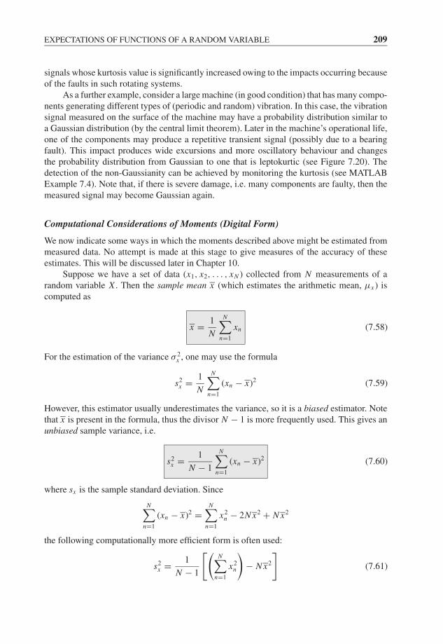
JWBK207-07 JWBK207-Shin January 26, 2008 17:21 Char Count= 0
EXPECTATIONS OF FUNCTIONS OF A RANDOM VARIABLE 209
signals whose kurtosis value is significantly increased owing to the impacts occurring becauseof the faults in such rotating systems.
As a further example, consider a large machine (in good condition) that has many compo-nents generating different types of (periodic and random) vibration. In this case, the vibrationsignal measured on the surface of the machine may have a probability distribution similar toa Gaussian distribution (by the central limit theorem). Later in the machine’s operational life,one of the components may produce a repetitive transient signal (possibly due to a bearingfault). This impact produces wide excursions and more oscillatory behaviour and changesthe probability distribution from Gaussian to one that is leptokurtic (see Figure 7.20). Thedetection of the non-Gaussianity can be achieved by monitoring the kurtosis (see MATLABExample 7.4). Note that, if there is severe damage, i.e. many components are faulty, then themeasured signal may become Gaussian again.
Computational Considerations of Moments (Digital Form)
We now indicate some ways in which the moments described above might be estimated frommeasured data. No attempt is made at this stage to give measures of the accuracy of theseestimates. This will be discussed later in Chapter 10.
Suppose we have a set of data (x1, x2, . . . , xN ) collected from N measurements of arandom variable X . Then the sample mean x (which estimates the arithmetic mean, μx ) iscomputed as
x = 1
N
N∑n=1
xn (7.58)
For the estimation of the variance σ 2x , one may use the formula
s2x = 1
N
N∑n=1
(xn − x)2 (7.59)
However, this estimator usually underestimates the variance, so it is a biased estimator. Notethat x is present in the formula, thus the divisor N − 1 is more frequently used. This gives anunbiased sample variance, i.e.
s2x = 1
N − 1
N∑n=1
(xn − x)2 (7.60)
where sx is the sample standard deviation. Since
N∑n=1
(xn − x)2 =N∑
n=1
x2n − 2N x2 + N x2
the following computationally more efficient form is often used:
s2x = 1
N − 1
[(N∑
n=1
x2n
)− N x2
](7.61)
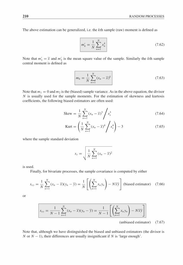
JWBK207-07 JWBK207-Shin January 26, 2008 17:21 Char Count= 0
210 RANDOM PROCESSES
The above estimation can be generalized, i.e. the kth sample (raw) moment is defined as
m ′k = 1
N
N∑n=1
xkn (7.62)
Note that m ′1 = x and m ′
2 is the mean square value of the sample. Similarly the kth samplecentral moment is defined as
mk = 1
N
N∑n=1
(xn − x)k (7.63)
Note that m1 = 0 and m2 is the (biased) sample variance. As in the above equation, the divisorN is usually used for the sample moments. For the estimation of skewness and kurtosiscoefficients, the following biased estimators are often used:
Skew = 1
N
N∑n=1
(xn − x)3
/s3
x (7.64)
Kurt =(
1
N
N∑n=1
(xn − x)4
/s4
x
)− 3 (7.65)
where the sample standard deviation
sx =√√√√ 1
N
N∑n=1
(xn − x)2
is used.Finally, for bivariate processes, the sample covariance is computed by either
sxy = 1
N
N∑n=1
(xn − x)(yn − y) = 1
N
[(N∑
n=1
xn yn
)− N xy
](biased estimator) (7.66)
or
sxy = 1
N − 1
N∑n=1
(xn − x)(yn − y) = 1
N − 1
[(N∑
n=1
xn yn
)− N xy
]
(unbiased estimator) (7.67)
Note that, although we have distinguished the biased and unbiased estimators (the divisor isN or N − 1), their differences are usually insignificant if N is ‘large enough’.
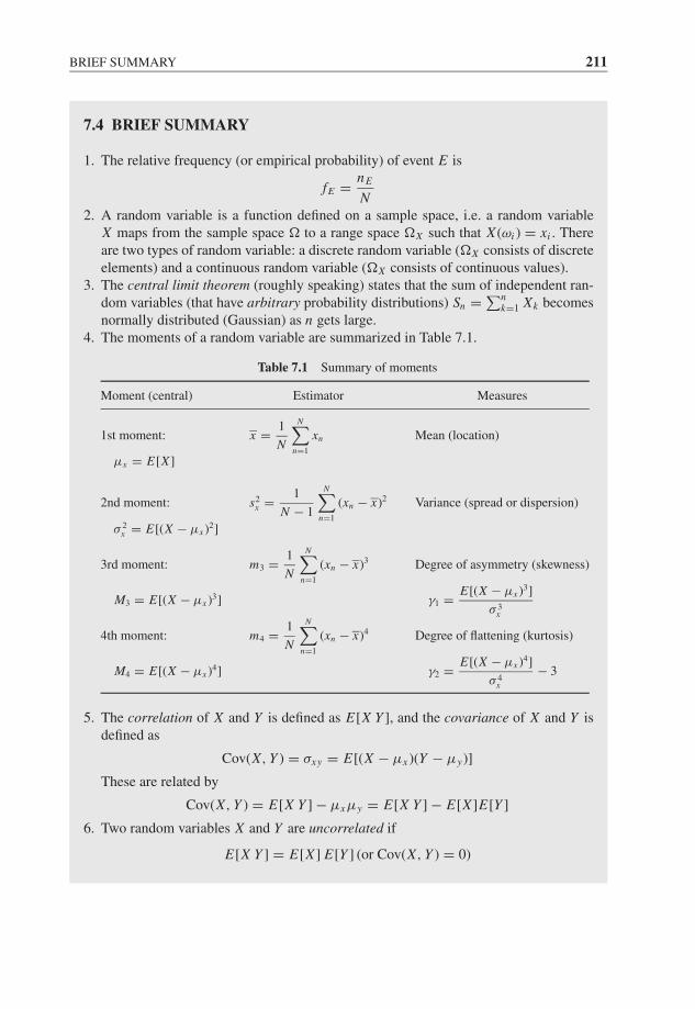
JWBK207-07 JWBK207-Shin January 26, 2008 17:21 Char Count= 0
BRIEF SUMMARY 211
7.4 BRIEF SUMMARY
1. The relative frequency (or empirical probability) of event E is
fE = nE
N2. A random variable is a function defined on a sample space, i.e. a random variable
X maps from the sample space � to a range space �X such that X (ωi ) = xi . Thereare two types of random variable: a discrete random variable (�X consists of discreteelements) and a continuous random variable (�X consists of continuous values).
3. The central limit theorem (roughly speaking) states that the sum of independent ran-dom variables (that have arbitrary probability distributions) Sn = ∑n
k=1 Xk becomesnormally distributed (Gaussian) as n gets large.
4. The moments of a random variable are summarized in Table 7.1.
Table 7.1 Summary of moments
Moment (central) Estimator Measures
1st moment: x = 1
N
N∑n=1
xn Mean (location)
μx = E[X ]
2nd moment: s2x = 1
N − 1
N∑n=1
(xn − x)2 Variance (spread or dispersion)
σ 2x = E[(X − μx )2]
3rd moment: m3 = 1
N
N∑n=1
(xn − x)3 Degree of asymmetry (skewness)
M3 = E[(X − μx )3] γ1 = E[(X − μx )3]
σ 3x
4th moment: m4 = 1
N
N∑n=1
(xn − x)4 Degree of flattening (kurtosis)
M4 = E[(X − μx )4] γ2 = E[(X − μx )4]
σ 4x
− 3
5. The correlation of X and Y is defined as E[X Y ], and the covariance of X and Y isdefined as
Cov(X, Y ) = σxy = E[(X − μx )(Y − μy)]
These are related by
Cov(X, Y ) = E[X Y ] − μxμy = E[X Y ] − E[X ]E[Y ]
6. Two random variables X and Y are uncorrelated if
E[X Y ] = E[X ] E[Y ] (or Cov(X, Y ) = 0)
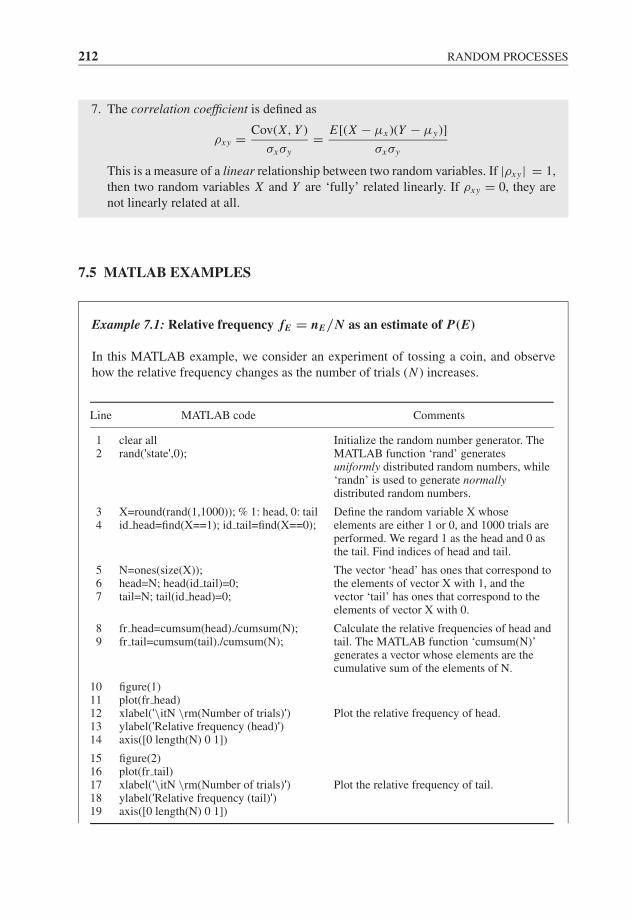
JWBK207-07 JWBK207-Shin January 26, 2008 17:21 Char Count= 0
212 RANDOM PROCESSES
7. The correlation coefficient is defined as
ρxy = Cov(X, Y )
σxσy= E[(X − μx )(Y − μy)]
σxσy
This is a measure of a linear relationship between two random variables. If |ρxy | = 1,then two random variables X and Y are ‘fully’ related linearly. If ρxy = 0, they arenot linearly related at all.
7.5 MATLAB EXAMPLES
Example 7.1: Relative frequency fE = nE/N as an estimate of P(E)
In this MATLAB example, we consider an experiment of tossing a coin, and observehow the relative frequency changes as the number of trials (N ) increases.
Line MATLAB code Comments
12
clear allrand('state',0);
Initialize the random number generator. TheMATLAB function ‘rand’ generatesuniformly distributed random numbers, while‘randn’ is used to generate normallydistributed random numbers.
34
X=round(rand(1,1000)); % 1: head, 0: tailid head=find(X==1); id tail=find(X==0);
Define the random variable X whoseelements are either 1 or 0, and 1000 trials areperformed. We regard 1 as the head and 0 asthe tail. Find indices of head and tail.
567
N=ones(size(X));head=N; head(id tail)=0;tail=N; tail(id head)=0;
The vector ‘head’ has ones that correspond tothe elements of vector X with 1, and thevector ‘tail’ has ones that correspond to theelements of vector X with 0.
89
fr head=cumsum(head)./cumsum(N);fr tail=cumsum(tail)./cumsum(N);
Calculate the relative frequencies of head andtail. The MATLAB function ‘cumsum(N)’generates a vector whose elements are thecumulative sum of the elements of N.
10 figure(1)11 plot(fr head)12 xlabel('\itN \rm(Number of trials)') Plot the relative frequency of head.13 ylabel('Relative frequency (head)')14 axis([0 length(N) 0 1])
15 figure(2)16 plot(fr tail)17 xlabel('\itN \rm(Number of trials)') Plot the relative frequency of tail.18 ylabel('Relative frequency (tail)')19 axis([0 length(N) 0 1])
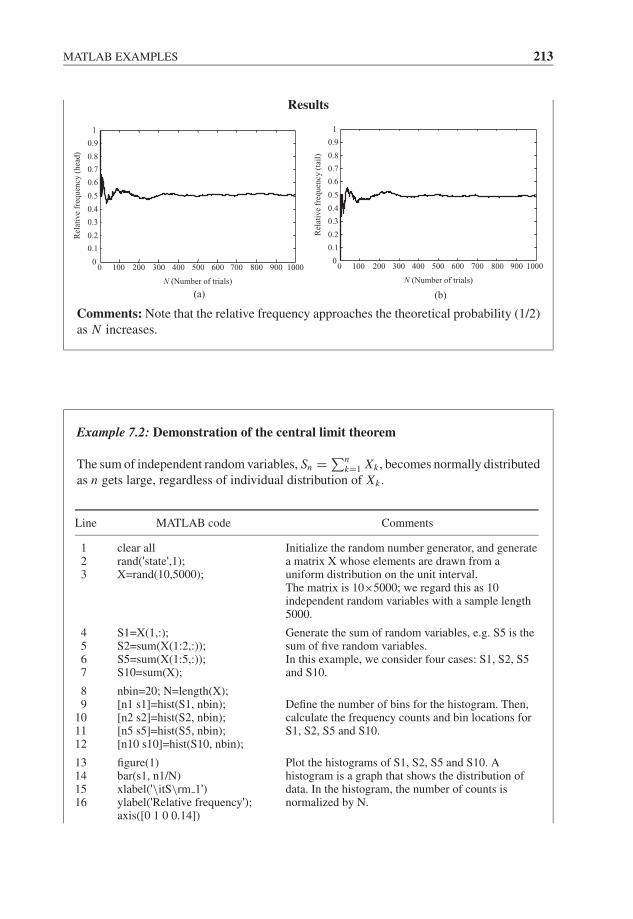
JWBK207-07 JWBK207-Shin January 26, 2008 17:21 Char Count= 0
MATLAB EXAMPLES 213
Results
0 100 200 300 400 500 600 700 800 900 10000
0.1
0.2
0.3
0.4
0.5
0.6
0.7
0.8
0.9
1
N (Number of trials)
Rel
ativ
e fr
equ
ency
(h
ead
)
(a)
0 100 200 300 400 500 600 700 800 900 10000
0.1
0.2
0.3
0.4
0.5
0.6
0.7
0.8
0.9
1
Rel
ativ
e fr
equ
ency
(ta
il)
N (Number of trials)
(b)
Comments: Note that the relative frequency approaches the theoretical probability (1/2)as N increases.
Example 7.2: Demonstration of the central limit theorem
The sum of independent random variables, Sn = ∑nk=1 Xk , becomes normally distributed
as n gets large, regardless of individual distribution of Xk .
Line MATLAB code Comments
123
clear allrand('state',1);X=rand(10,5000);
Initialize the random number generator, and generatea matrix X whose elements are drawn from auniform distribution on the unit interval.The matrix is 10×5000; we regard this as 10independent random variables with a sample length5000.
4567
S1=X(1,:);S2=sum(X(1:2,:));S5=sum(X(1:5,:));S10=sum(X);
Generate the sum of random variables, e.g. S5 is thesum of five random variables.In this example, we consider four cases: S1, S2, S5and S10.
89
101112
nbin=20; N=length(X);[n1 s1]=hist(S1, nbin);[n2 s2]=hist(S2, nbin);[n5 s5]=hist(S5, nbin);[n10 s10]=hist(S10, nbin);
Define the number of bins for the histogram. Then,calculate the frequency counts and bin locations forS1, S2, S5 and S10.
13 figure(1) Plot the histograms of S1, S2, S5 and S10. A14 bar(s1, n1/N) histogram is a graph that shows the distribution of15 xlabel('\itS\rm 1') data. In the histogram, the number of counts is16 ylabel('Relative frequency'); normalized by N.
axis([0 1 0 0.14])
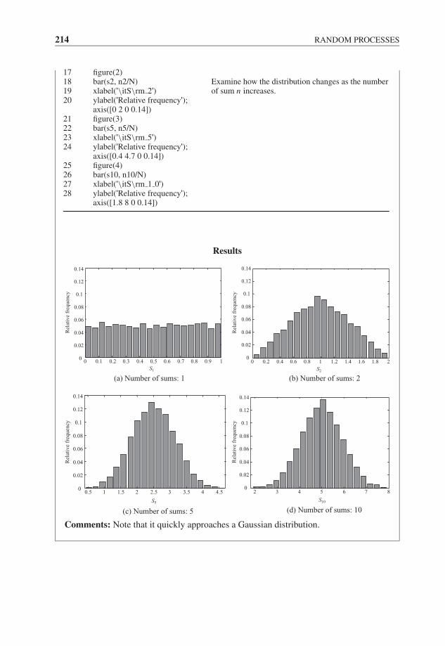
JWBK207-07 JWBK207-Shin January 26, 2008 17:21 Char Count= 0
214 RANDOM PROCESSES
17 figure(2)18 bar(s2, n2/N) Examine how the distribution changes as the number19 xlabel('\itS\rm 2') of sum n increases.20 ylabel('Relative frequency');
axis([0 2 0 0.14])21 figure(3)22 bar(s5, n5/N)23 xlabel('\itS\rm 5')24 ylabel('Relative frequency');
axis([0.4 4.7 0 0.14])25 figure(4)26 bar(s10, n10/N)27 xlabel('\itS\rm 1 0')28 ylabel('Relative frequency');
axis([1.8 8 0 0.14])
Results
0 0.1 0.2 0.3 0.4 0.5
(a) Number of sums: 1
0.6 0.7 0.8 0.9 10
0.02
0.04
0.06
0.08
0.1
0.12
0.14
S1
Rel
ativ
e fr
equ
ency
(b) Number of sums: 2
0 0.2 0.4 0.6 0.8 1 1.2 1.4 1.6 1.8 20
0.02
0.04
0.06
0.08
0.1
0.12
0.14
Rel
ativ
e fr
equ
ency
S2
(c) Number of sums: 5
S5
0.5 1 1.5 2 2.5 3 3.5 4 4.50
0.02
0.04
0.06
0.08
0.1
0.12
0.14
Rel
ativ
e fr
equen
cy
(d) Number of sums: 10
S10
2 3 4 5 6 870
0.02
0.04
0.06
0.08
0.1
0.12
0.14
Rel
ativ
e fr
equen
cy
Comments: Note that it quickly approaches a Gaussian distribution.
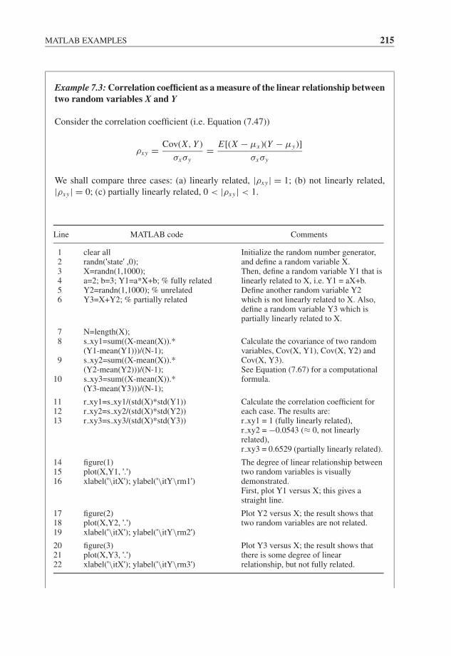
JWBK207-07 JWBK207-Shin January 26, 2008 17:21 Char Count= 0
MATLAB EXAMPLES 215
Example 7.3: Correlation coefficient as a measure of the linear relationship betweentwo random variables X and Y
Consider the correlation coefficient (i.e. Equation (7.47))
ρxy = Cov(X, Y )
σxσy= E[(X − μx )(Y − μy)]
σxσy
We shall compare three cases: (a) linearly related, |ρxy | = 1; (b) not linearly related,|ρxy | = 0; (c) partially linearly related, 0 < |ρxy | < 1.
Line MATLAB code Comments
123456
clear allrandn('state' ,0);X=randn(1,1000);a=2; b=3; Y1=a*X+b; % fully relatedY2=randn(1,1000); % unrelatedY3=X+Y2; % partially related
Initialize the random number generator,and define a random variable X.Then, define a random variable Y1 that islinearly related to X, i.e. Y1 = aX+b.Define another random variable Y2which is not linearly related to X. Also,define a random variable Y3 which ispartially linearly related to X.
78
9
10
N=length(X);s xy1=sum((X-mean(X)).*(Y1-mean(Y1)))/(N-1);s xy2=sum((X-mean(X)).*(Y2-mean(Y2)))/(N-1);s xy3=sum((X-mean(X)).*(Y3-mean(Y3)))/(N-1);
Calculate the covariance of two randomvariables, Cov(X, Y1), Cov(X, Y2) andCov(X, Y3).See Equation (7.67) for a computationalformula.
111213
r xy1=s xy1/(std(X)*std(Y1))r xy2=s xy2/(std(X)*std(Y2))r xy3=s xy3/(std(X)*std(Y3))
Calculate the correlation coefficient foreach case. The results are:r xy1 = 1 (fully linearly related),r xy2 = −0.0543 (≈ 0, not linearlyrelated),r xy3 = 0.6529 (partially linearly related).
141516
figure(1)plot(X,Y1, '.')xlabel('\itX'); ylabel('\itY\rm1')
The degree of linear relationship betweentwo random variables is visuallydemonstrated.First, plot Y1 versus X; this gives astraight line.
171819
figure(2)plot(X,Y2, '.')xlabel('\itX'); ylabel('\itY\rm2')
Plot Y2 versus X; the result shows thattwo random variables are not related.
202122
figure(3)plot(X,Y3, '.')xlabel('\itX'); ylabel('\itY\rm3')
Plot Y3 versus X; the result shows thatthere is some degree of linearrelationship, but not fully related.
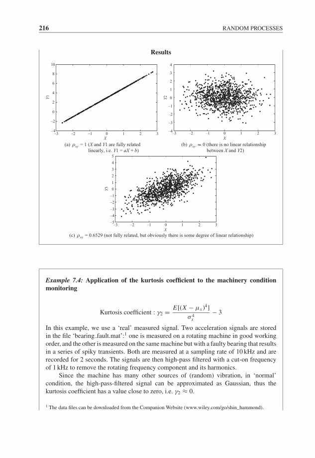
JWBK207-07 JWBK207-Shin January 26, 2008 17:21 Char Count= 0
216 RANDOM PROCESSES
Results
–3 –2 –1 0 1 32–4
–3
–2
–1
0
1
2
3
4
XX
Y2
(a) ρxy = 1 (X and Y1 are fully related
linearly, i.e. Y1 = aX + b)
(c) ρxy = 0.6529 (not fully related, but obviously there is some degree of linear relationship)
(b) ρxy ∼ 0 (there is no linear relationship
between X and Y2)
10
–3 –2 –1 0 1 32–4
–2
0
2
4
6
8
Y1
–3 –2 –1 0 1 32–5
–4
–3
–2
–1
0
1
2
3
4
5
X
Y3
∼
Example 7.4: Application of the kurtosis coefficient to the machinery conditionmonitoring
Kurtosis coefficient : γ2 = E[(X − μx )4]
σ 4x
− 3
In this example, we use a ‘real’ measured signal. Two acceleration signals are storedin the file ‘bearing fault.mat’:1 one is measured on a rotating machine in good workingorder, and the other is measured on the same machine but with a faulty bearing that resultsin a series of spiky transients. Both are measured at a sampling rate of 10 kHz and arerecorded for 2 seconds. The signals are then high-pass filtered with a cut-on frequencyof 1 kHz to remove the rotating frequency component and its harmonics.
Since the machine has many other sources of (random) vibration, in ‘normal’condition, the high-pass-filtered signal can be approximated as Gaussian, thus thekurtosis coefficient has a value close to zero, i.e. γ2 ≈ 0.
1 The data files can be downloaded from the Companion Website (www.wiley.com/go/shin hammond).
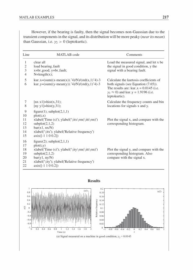
JWBK207-07 JWBK207-Shin January 26, 2008 17:21 Char Count= 0
MATLAB EXAMPLES 217
However, if the bearing is faulty, then the signal becomes non-Gaussian due to thetransient components in the signal, and its distribution will be more peaky (near its mean)than Gaussian, i.e. γ2 > 0 (leptokurtic).
Line MATLAB code Comments
1234
clear allload bearing faultx=br good; y=br fault;N=length(x);
Load the measured signal, and let x bethe signal in good condition, y thesignal with a bearing fault.
56
kur x=(sum((x-mean(x)).ˆ4)/N)/(std(x,1)ˆ4)-3kur y=(sum((y-mean(y)).ˆ4)/N)/(std(y,1)ˆ4)-3
Calculate the kurtosis coefficients ofboth signals (see Equation (7.65)).The results are: kur x = 0.0145 (i.e.γ2 ≈ 0) and kur y = 1.9196 (i.e.leptokurtic).
78
[nx x1]=hist(x,31);[ny y1]=hist(y,31);
Calculate the frequency counts and binlocations for signals x and y.
9101112131415
figure(1); subplot(2,1,1)plot(t,x)xlabel('Time (s)'); ylabel('\itx\rm(\itt\rm)')subplot(2,1,2)bar(x1, nx/N)xlabel('\itx'); ylabel('Relative frequency')axis([-1 1 0 0.2])
Plot the signal x, and compare with thecorresponding histogram.
16171819202122
figure(2); subplot(2,1,1)plot(t,y)xlabel('Time (s)'); ylabel('\ity\rm(\itt\rm)')subplot(2,1,2)bar(y1, ny/N)xlabel('\ity'); ylabel('Relative frequency')axis([-1 1 0 0.2])
Plot the signal y, and compare with thecorresponding histogram. Alsocompare with the signal x.
Results
(a) Signal measured on a machine in good condition, γ2 = 0.0145
0 0.2 0.4 0.6 0.8 1 1.2 1.4 1.6 1.8 2–1
–0.8
–0.6
–0.4
–0.2
0
0.2
0.4
0.6
0.8
1
Time (s)
x(t)
–1 –0.8 –0.6 –0.4 –0.2 0 0.2 0.4 0.6 0.8 10
0.02
0.04
0.06
0.08
0.1
0.12
0.14
0.16
0.18
0.2
x
Rel
ativ
e fr
equen
cy
(a1) (a2)
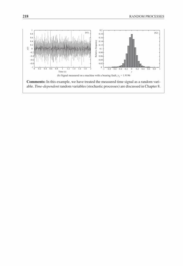
JWBK207-07 JWBK207-Shin January 26, 2008 17:21 Char Count= 0
218 RANDOM PROCESSES
(b) Signal measured on a machine with a bearing fault, γ2 = 1.9196
0 0.2 0.4 0.6 0.8 1 1.2 1.4 1.6 1.8 2–1
–0.8
–0.6
–0.4
–0.2
0
0.2
0.4
0.6
0.8
1
Time (s)
y(t)
–1 –0.8 –0.6 –0.4 –0.2 0 0.2 0.4 0.6 0.8 10
0.02
0.04
0.06
0.08
0.1
0.12
0.14
0.16
0.18
0.2
y
Rel
ativ
e fr
equen
cy
(b1) (b2)
Comments: In this example, we have treated the measured time signal as a random vari-able. Time-dependent random variables (stochastic processes) are discussed in Chapter 8.
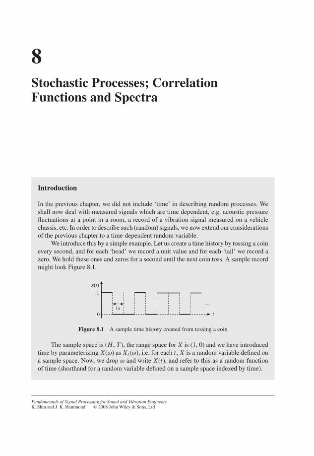
JWBK207-08 JWBK207-Shin January 18, 2008 10:6 Char Count= 0
8Stochastic Processes; CorrelationFunctions and Spectra
Introduction
In the previous chapter, we did not include ‘time’ in describing random processes. Weshall now deal with measured signals which are time dependent, e.g. acoustic pressurefluctuations at a point in a room, a record of a vibration signal measured on a vehiclechassis, etc. In order to describe such (random) signals, we now extend our considerationsof the previous chapter to a time-dependent random variable.
We introduce this by a simple example. Let us create a time history by tossing a coinevery second, and for each ‘head’ we record a unit value and for each ‘tail’ we record azero. We hold these ones and zeros for a second until the next coin toss. A sample recordmight look Figure 8.1.
x(t)
t
...
0
1
1s
Figure 8.1 A sample time history created from tossing a coin
The sample space is (H , T ), the range space for X is (1, 0) and we have introducedtime by parameterizing X (ω) as Xt (ω), i.e. for each t , X is a random variable defined ona sample space. Now, we drop ω and write X (t), and refer to this as a random functionof time (shorthand for a random variable defined on a sample space indexed by time).
Fundamentals of Signal Processing for Sound and Vibration EngineersK. Shin and J. K. Hammond. C© 2008 John Wiley & Sons, Ltd
219
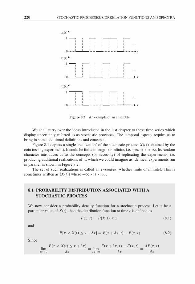
JWBK207-08 JWBK207-Shin January 18, 2008 10:6 Char Count= 0
220 STOCHASTIC PROCESSES; CORRELATION FUNCTIONS AND SPECTRA
1( )x t
2 ( )x t
( )nx t
0
1
0
1
0
1
...
...
...
t
t
t
......
Figure 8.2 An example of an ensemble
We shall carry over the ideas introduced in the last chapter to these time series whichdisplay uncertainty referred to as stochastic processes. The temporal aspects require us tobring in some additional definitions and concepts.
Figure 8.1 depicts a single ‘realization’ of the stochastic process X (t) (obtained by thecoin tossing experiment). It could be finite in length or infinite, i.e. −∞ < t < ∞. Its randomcharacter introduces us to the concepts (or necessity) of replicating the experiments, i.e.producing additional realizations of it, which we could imagine as identical experiments runin parallel as shown in Figure 8.2.
The set of such realizations is called an ensemble (whether finite or infinite). This issometimes written as {X (t)} where −∞ < t < ∞.
8.1 PROBABILITY DISTRIBUTION ASSOCIATED WITH ASTOCHASTIC PROCESS
We now consider a probability density function for a stochastic process. Let x be aparticular value of X (t); then the distribution function at time t is defined as
F(x, t) = P[X (t) ≤ x] (8.1)
and
P[x < X (t) ≤ x + δx] = F(x + δx, t) − F(x, t) (8.2)
Since
limδx→0
P[x < X (t) ≤ x + δx]
δx= lim
δx→0
F(x + δx, t) − F(x, t)
δx= d F(x, t)
dx
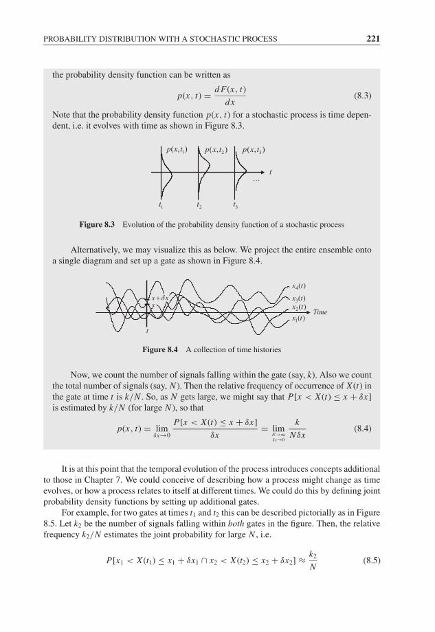
JWBK207-08 JWBK207-Shin January 18, 2008 10:6 Char Count= 0
PROBABILITY DISTRIBUTION WITH A STOCHASTIC PROCESS 221
the probability density function can be written as
p(x, t) = d F(x, t)
dx(8.3)
Note that the probability density function p(x, t) for a stochastic process is time depen-dent, i.e. it evolves with time as shown in Figure 8.3.
1( , )p x t2( , )p x t 3( , )p x t
...
3t2t1t
t
Figure 8.3 Evolution of the probability density function of a stochastic process
Alternatively, we may visualize this as below. We project the entire ensemble ontoa single diagram and set up a gate as shown in Figure 8.4.
x xδ+x
1( )x t2( )x t3( )x t
4( )x t
t
Time
Figure 8.4 A collection of time histories
Now, we count the number of signals falling within the gate (say, k). Also we countthe total number of signals (say, N ). Then the relative frequency of occurrence of X (t) inthe gate at time t is k/N . So, as N gets large, we might say that P[x < X (t) ≤ x + δx]is estimated by k/N (for large N ), so that
p(x, t) = limδx→0
P[x < X (t) ≤ x + δx]
δx= lim
N→∞δx→0
k
Nδx(8.4)
It is at this point that the temporal evolution of the process introduces concepts additionalto those in Chapter 7. We could conceive of describing how a process might change as timeevolves, or how a process relates to itself at different times. We could do this by defining jointprobability density functions by setting up additional gates.
For example, for two gates at times t1 and t2 this can be described pictorially as in Figure8.5. Let k2 be the number of signals falling within both gates in the figure. Then, the relativefrequency k2/N estimates the joint probability for large N , i.e.
P[x1 < X (t1) ≤ x1 + δx1 ∩ x2 < X (t2) ≤ x2 + δx2] ≈ k2
N(8.5)

JWBK207-08 JWBK207-Shin January 18, 2008 10:6 Char Count= 0
222 STOCHASTIC PROCESSES; CORRELATION FUNCTIONS AND SPECTRA
1 1x xδ+
1x
1( )x t2( )x t3( )x t
4( )x t
1t
2 2x xδ+
2x
2t
Time
Figure 8.5 Pictorial description of the joint probability density function
Thus, the joint probability density function is written as
p(x1, t1; x2, t2) = limδx1,δx2→0
P[x1 < X (t1) ≤ x1 + δx1 ∩ x2 < X (t2) ≤ x2 + δx2]
δx1δx2
= limN→∞
δx1 ,δx2→0
k2
Nδx1δx2
(8.6)
Also, the joint distribution function is F(x1, t1; x2, t2) = P[X (t1) ≤ x1 ∩ X (t2) ≤ x2], soEquation (8.6) can be rewritten as
p(x1, t1; x2, t2) = ∂2 F(x1, t1; x2, t2)
∂x1∂x2
(8.7)
For a ‘univariate’ stochastic process, Equation (8.7) can be generalized to the kth-orderjoint probability density function as
p(x1, t1; x2, t2; . . . ; xk, tk) (8.8)
However, we shall only consider the first and second order, i.e. p(x, t) and p(x1, t1; x2, t2).
8.2 MOMENTS OF A STOCHASTIC PROCESS
As we have defined the moments for random variables in Chapter 7, we now definemoments for stochastic processes. The only difference is that ‘time’ is involved now, i.e.the moments of a stochastic process are time dependent. The first and second momentsare as follows:
(a) First moment (mean):
μx (t) = E[X (t)] =∞∫
−∞xp(x, t)dx (8.9)
(b) Second moment (mean square):
E[X2(t)] =∞∫
−∞x2 p(x, t)dx (8.10)
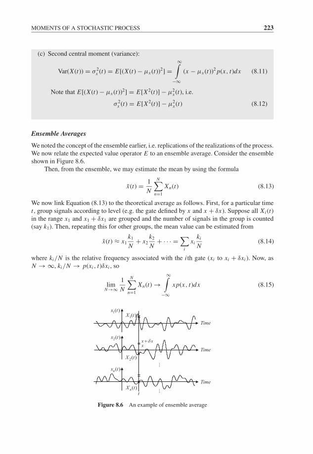
JWBK207-08 JWBK207-Shin January 18, 2008 10:6 Char Count= 0
MOMENTS OF A STOCHASTIC PROCESS 223
(c) Second central moment (variance):
Var(X (t)) = σ 2x (t) = E[(X (t) − μx (t))2] =
∞∫−∞
(x − μx (t))2 p(x, t)dx (8.11)
Note that E[(X (t) − μx (t))2] = E[X2(t)] − μ2x (t), i.e.
σ 2x (t) = E[X2(t)] − μ2
x (t) (8.12)
Ensemble Averages
We noted the concept of the ensemble earlier, i.e. replications of the realizations of the process.We now relate the expected value operator E to an ensemble average. Consider the ensembleshown in Figure 8.6.
Then, from the ensemble, we may estimate the mean by using the formula
x(t) = 1
N
N∑n=1
Xn(t) (8.13)
We now link Equation (8.13) to the theoretical average as follows. First, for a particular timet , group signals according to level (e.g. the gate defined by x and x + δx). Suppose all Xi (t)in the range x1 and x1 + δx1 are grouped and the number of signals in the group is counted(say k1). Then, repeating this for other groups, the mean value can be estimated from
x(t) ≈ x1
k1
N+ x2
k2
N+ · · · =
∑i
xiki
N(8.14)
where ki/N is the relative frequency associated with the i th gate (xi to xi + δxi ). Now, asN → ∞, ki/N → p(xi , t)δxi , so
limN→∞
1
N
N∑n=1
Xn(t) →∞∫
−∞xp(x, t)dx (8.15)
1( )x t
2( )x t
( )nx t
1( )X t
2( )X t
( )nX t
xx xδ+
...
...
Time
Time
Time
t
Figure 8.6 An example of ensemble average
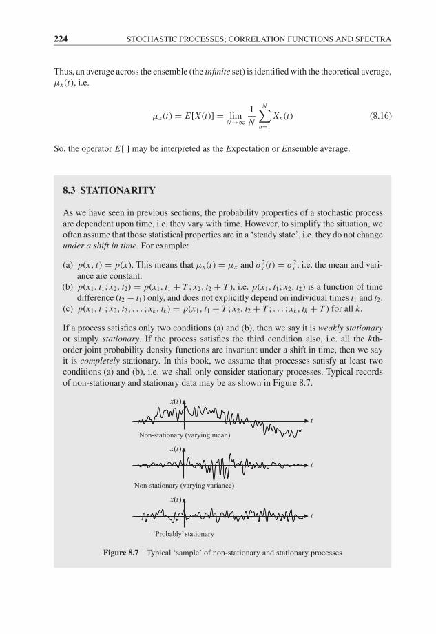
JWBK207-08 JWBK207-Shin January 18, 2008 10:6 Char Count= 0
224 STOCHASTIC PROCESSES; CORRELATION FUNCTIONS AND SPECTRA
Thus, an average across the ensemble (the infinite set) is identified with the theoretical average,μx (t), i.e.
μx (t) = E[X (t)] = limN→∞
1
N
N∑n=1
Xn(t) (8.16)
So, the operator E[ ] may be interpreted as the Expectation or Ensemble average.
8.3 STATIONARITY
As we have seen in previous sections, the probability properties of a stochastic processare dependent upon time, i.e. they vary with time. However, to simplify the situation, weoften assume that those statistical properties are in a ‘steady state’, i.e. they do not changeunder a shift in time. For example:
(a) p(x, t) = p(x). This means that μx (t) = μx and σ 2x (t) = σ 2
x , i.e. the mean and vari-ance are constant.
(b) p(x1, t1; x2, t2) = p(x1, t1 + T ; x2, t2 + T ), i.e. p(x1, t1; x2, t2) is a function of timedifference (t2 − t1) only, and does not explicitly depend on individual times t1 and t2.
(c) p(x1, t1; x2, t2; . . . ; xk, tk) = p(x1, t1 + T ; x2, t2 + T ; . . . ; xk, tk + T ) for all k.
If a process satisfies only two conditions (a) and (b), then we say it is weakly stationaryor simply stationary. If the process satisfies the third condition also, i.e. all the kth-order joint probability density functions are invariant under a shift in time, then we sayit is completely stationary. In this book, we assume that processes satisfy at least twoconditions (a) and (b), i.e. we shall only consider stationary processes. Typical recordsof non-stationary and stationary data may be as shown in Figure 8.7.
( )x t
Non-stationary (varying variance)
Non-stationary (varying mean)
‘Probably’stationary
( )x t
( )x t
t
t
t
Figure 8.7 Typical ‘sample’ of non-stationary and stationary processes
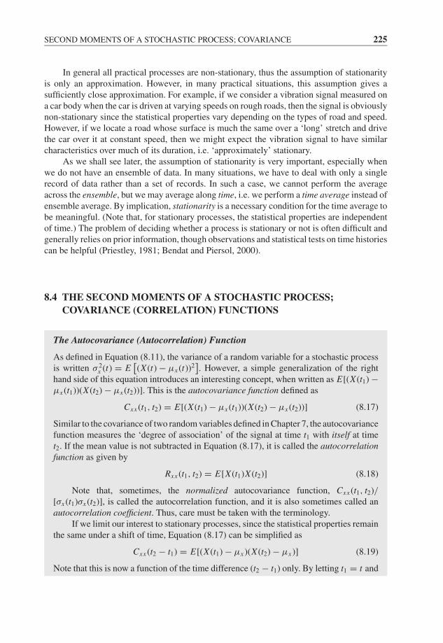
JWBK207-08 JWBK207-Shin January 18, 2008 10:6 Char Count= 0
SECOND MOMENTS OF A STOCHASTIC PROCESS; COVARIANCE 225
In general all practical processes are non-stationary, thus the assumption of stationarityis only an approximation. However, in many practical situations, this assumption gives asufficiently close approximation. For example, if we consider a vibration signal measured ona car body when the car is driven at varying speeds on rough roads, then the signal is obviouslynon-stationary since the statistical properties vary depending on the types of road and speed.However, if we locate a road whose surface is much the same over a ‘long’ stretch and drivethe car over it at constant speed, then we might expect the vibration signal to have similarcharacteristics over much of its duration, i.e. ‘approximately’ stationary.
As we shall see later, the assumption of stationarity is very important, especially whenwe do not have an ensemble of data. In many situations, we have to deal with only a singlerecord of data rather than a set of records. In such a case, we cannot perform the averageacross the ensemble, but we may average along time, i.e. we perform a time average instead ofensemble average. By implication, stationarity is a necessary condition for the time average tobe meaningful. (Note that, for stationary processes, the statistical properties are independentof time.) The problem of deciding whether a process is stationary or not is often difficult andgenerally relies on prior information, though observations and statistical tests on time historiescan be helpful (Priestley, 1981; Bendat and Piersol, 2000).
8.4 THE SECOND MOMENTS OF A STOCHASTIC PROCESS;COVARIANCE (CORRELATION) FUNCTIONS
The Autocovariance (Autocorrelation) Function
As defined in Equation (8.11), the variance of a random variable for a stochastic processis written σ 2
x (t) = E[(X (t) − μx (t))2
]. However, a simple generalization of the right
hand side of this equation introduces an interesting concept, when written as E[(X (t1) −μx (t1))(X (t2) − μx (t2))]. This is the autocovariance function defined as
Cxx (t1, t2) = E[(X (t1) − μx (t1))(X (t2) − μx (t2))] (8.17)
Similar to the covariance of two random variables defined in Chapter 7, the autocovariancefunction measures the ‘degree of association’ of the signal at time t1 with itself at timet2. If the mean value is not subtracted in Equation (8.17), it is called the autocorrelationfunction as given by
Rxx (t1, t2) = E[X (t1)X (t2)] (8.18)
Note that, sometimes, the normalized autocovariance function, Cxx (t1, t2)/[σx (t1)σx (t2)], is called the autocorrelation function, and it is also sometimes called anautocorrelation coefficient. Thus, care must be taken with the terminology.
If we limit our interest to stationary processes, since the statistical properties remainthe same under a shift of time, Equation (8.17) can be simplified as
Cxx (t2 − t1) = E[(X (t1) − μx )(X (t2) − μx )] (8.19)
Note that this is now a function of the time difference (t2 − t1) only. By letting t1 = t and
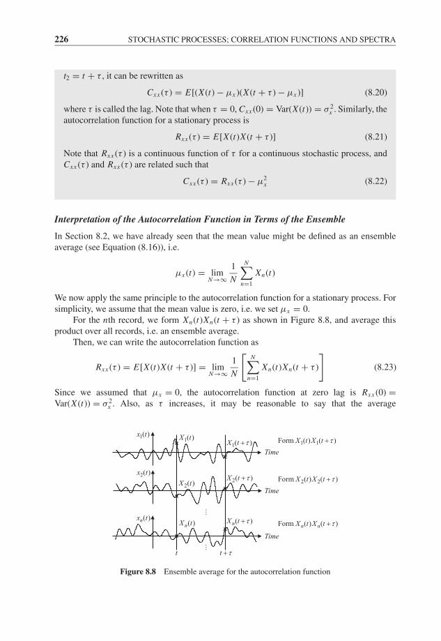
JWBK207-08 JWBK207-Shin January 18, 2008 10:6 Char Count= 0
226 STOCHASTIC PROCESSES; CORRELATION FUNCTIONS AND SPECTRA
t2 = t + τ , it can be rewritten as
Cxx (τ ) = E[(X (t) − μx )(X (t + τ ) − μx )] (8.20)
where τ is called the lag. Note that when τ = 0, Cxx (0) = Var(X (t)) = σ 2x . Similarly, the
autocorrelation function for a stationary process is
Rxx (τ ) = E[X (t)X (t + τ )] (8.21)
Note that Rxx (τ ) is a continuous function of τ for a continuous stochastic process, andCxx (τ ) and Rxx (τ ) are related such that
Cxx (τ ) = Rxx (τ ) − μ2x (8.22)
Interpretation of the Autocorrelation Function in Terms of the Ensemble
In Section 8.2, we have already seen that the mean value might be defined as an ensembleaverage (see Equation (8.16)), i.e.
μx (t) = limN→∞
1
N
N∑n=1
Xn(t)
We now apply the same principle to the autocorrelation function for a stationary process. Forsimplicity, we assume that the mean value is zero, i.e. we set μx = 0.
For the nth record, we form Xn(t)Xn(t + τ ) as shown in Figure 8.8, and average thisproduct over all records, i.e. an ensemble average.
Then, we can write the autocorrelation function as
Rxx (τ ) = E[X (t)X (t + τ )] = limN→∞
1
N
[N∑
n=1
Xn(t)Xn(t + τ )
](8.23)
Since we assumed that μx = 0, the autocorrelation function at zero lag is Rxx (0) =Var(X (t)) = σ 2
x . Also, as τ increases, it may be reasonable to say that the average
1( )x t
2( )x t
( )nx t
...
...
Time
Time
Time
t
1( )X t τ+
2( )X t τ+
( )nX t τ+
1( )X t
2( )X t
( )nX t
1 1Form ( ) ( )X t X t τ+
2 2Form ( ) ( )X t X t τ+
Form ( ) ( )n nX t X t τ+
t τ+
Figure 8.8 Ensemble average for the autocorrelation function

JWBK207-08 JWBK207-Shin January 18, 2008 10:6 Char Count= 0
SECOND MOMENTS OF A STOCHASTIC PROCESS; COVARIANCE 227
2 (for zero mean)xσ
( )xxR τ
τ
Figure 8.9 A typical autocorrelation function
E[X (t)X (t + τ )] should approach zero, since the values of X (t) and X (t + τ ) for large lags(time separations) are ‘less associated (related)’ if the process is random. Thus, the gen-eral shape of the autocorrelation function Rxx (τ ) may be drawn as in Figure 8.9. Note that,as can be seen from the figure, the autocorrelation function is an even function of τ sinceE[X (t)X (t + τ )] = E[X (t − τ )X (t)].
We note that the autocorrelation function does not always decay to zero. An example ofwhen this does not happen is when the signal has a periodic form (see Section 8.6).
The Cross-covariance (Cross-correlation) Function
If we consider two stochastic processes {X (t)} and {Y (t)} simultaneously, e.g. aninput–output process, then we may generalize the above joint moment. Thus, the cross-covariance function is defined as
Cxy(t1, t2) = E[(X (t1) − μx (t1))(Y (t2) − μy(t2))] (8.24)
and, if the mean values are not subtracted, the cross-correlation function is defined as
Rxy(t1, t2) = E[X (t1)Y (t2)] (8.25)
Equation (8.24) or (8.25) is a measure of the association between the signal X (t) at timet1 and the signal Y (t) at time t2, i.e. it is a measure of cross-association. If we assumeboth signals are stationary, then Cxy(t1, t2) or Rxy(t1, t2) is a function of time differencet2 − t1. Then, as before, letting t1 = t and t2 = t + τ , the equations can be rewritten as
Cxy(τ ) = E[(X (t) − μx )(Y (t + τ ) − μy)] (8.26)
and
Rxy(τ ) = E[X (t)Y (t + τ )] (8.27)
where their relationship is
Cxy(τ ) = Rxy(τ ) − μxμy (8.28)
Also, the ensemble average interpretation becomes
Rxy(τ ) = E[X (t)Y (t + τ )] = limN→∞
1
N
[N∑
n=1
Xn(t)Yn(t + τ )
](8.29)
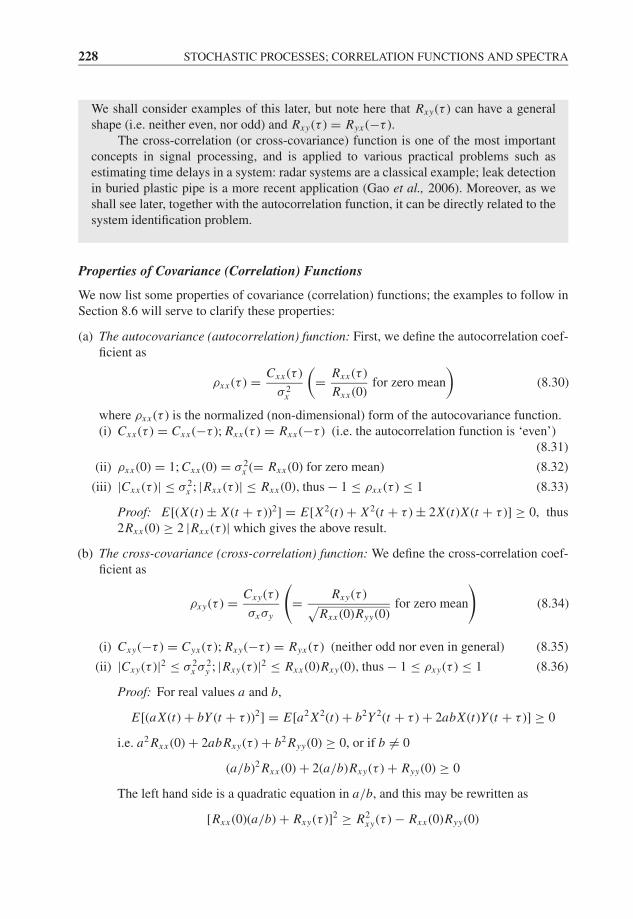
JWBK207-08 JWBK207-Shin January 18, 2008 10:6 Char Count= 0
228 STOCHASTIC PROCESSES; CORRELATION FUNCTIONS AND SPECTRA
We shall consider examples of this later, but note here that Rxy(τ ) can have a generalshape (i.e. neither even, nor odd) and Rxy(τ ) = Ryx (−τ ).
The cross-correlation (or cross-covariance) function is one of the most importantconcepts in signal processing, and is applied to various practical problems such asestimating time delays in a system: radar systems are a classical example; leak detectionin buried plastic pipe is a more recent application (Gao et al., 2006). Moreover, as weshall see later, together with the autocorrelation function, it can be directly related to thesystem identification problem.
Properties of Covariance (Correlation) Functions
We now list some properties of covariance (correlation) functions; the examples to follow inSection 8.6 will serve to clarify these properties:
(a) The autocovariance (autocorrelation) function: First, we define the autocorrelation coef-ficient as
ρxx (τ ) = Cxx (τ )
σ 2x
(= Rxx (τ )
Rxx (0)for zero mean
)(8.30)
where ρxx (τ ) is the normalized (non-dimensional) form of the autocovariance function.(i) Cxx (τ ) = Cxx (−τ ); Rxx (τ ) = Rxx (−τ ) (i.e. the autocorrelation function is ‘even’)
(8.31)
(ii) ρxx (0) = 1; Cxx (0) = σ 2x (= Rxx (0) for zero mean) (8.32)
(iii) |Cxx (τ )| ≤ σ 2x ; |Rxx (τ )| ≤ Rxx (0), thus − 1 ≤ ρxx (τ ) ≤ 1 (8.33)
Proof: E[(X (t) ± X (t + τ ))2] = E[X2(t) + X2(t + τ ) ± 2X (t)X (t + τ )] ≥ 0, thus2Rxx (0) ≥ 2 |Rxx (τ )| which gives the above result.
(b) The cross-covariance (cross-correlation) function: We define the cross-correlation coef-ficient as
ρxy(τ ) = Cxy(τ )
σxσy
(= Rxy(τ )√
Rxx (0)Ryy(0)for zero mean
)(8.34)
(i) Cxy(−τ ) = Cyx (τ ); Rxy(−τ ) = Ryx (τ ) (neither odd nor even in general) (8.35)
(ii) |Cxy(τ )|2 ≤ σ 2x σ 2
y ; |Rxy(τ )|2 ≤ Rxx (0)Rxy(0), thus − 1 ≤ ρxy(τ ) ≤ 1 (8.36)
Proof: For real values a and b,
E[(aX (t) + bY (t + τ ))2] = E[a2 X2(t) + b2Y 2(t + τ ) + 2abX (t)Y (t + τ )] ≥ 0
i.e. a2 Rxx (0) + 2abRxy(τ ) + b2 Ryy(0) ≥ 0, or if b = 0
(a/b)2 Rxx (0) + 2(a/b)Rxy(τ ) + Ryy(0) ≥ 0
The left hand side is a quadratic equation in a/b, and this may be rewritten as
[Rxx (0)(a/b) + Rxy(τ )]2 ≥ R2xy(τ ) − Rxx (0)Ryy(0)
JWBK207-08 JWBK207-Shin January 18, 2008 10:6 Char Count= 0
ERGODICITY AND TIME AVERAGES 229
For any values of a/b, this inequality must be satisfied. Thus
R2xy(τ ) − Rxx (0)Ryy(0) ≤ 0
and so the result follows.(iii) If X (t) and Y (t) are uncorrelated, Cxy(τ ) = 0; Rxy(τ ) = μxμy .
Note that the above correlation coefficients are particularly useful when X (t) and Y (t)have different scales. Although we have distinguished the covariance functions and correlationfunctions, their difference is the presence of mean values only. In most practical situations,the mean values are usually subtracted prior to some processing of data, so the correlationfunctions and the covariance functions are the same in effect. Consequently, the ‘correlation’functions are often preferably used in engineering.
8.5 ERGODICITY AND TIME AVERAGES
The moments discussed in previous sections are based on the theoretical probabilitydistributions of the stochastic processes and have been interpreted as ensemble averages,i.e. we need an infinite number of records whose statistical properties are identical.However, in general, ensemble averaging is not feasible as we usually have only a singlerealization (record) of limited length. Then, the only way to perform the average is alongthe time axis, i.e. a time average may be used in place of an ensemble average. Thequestion is: do time averages along one record give the same results as an ensembleaverage? The answer is ‘sometimes’, and when they do, such averages are said to beergodic.
Note that we cannot simply refer to a process as ergodic. Ergodicity must be relateddirectly to the particular average in question, e.g. mean value, autocorrelation functionand cross-correlation function, etc. Anticipating a result from statistical estimation theory,we can state that stationary processes are ergodic with respect to the mean and covariancefunctions. Thus, for example, the mean value can be written as
μx = limT →∞
1
T
T∫0
x(t)dt (8.37)
i.e. the time average over any single time history will give the same value as the ensembleaverage E[X (t)].
If we consider a signal with a finite length T , then the estimate of the mean valuecan be obtained by
μx = x = 1
T
T∫0
x(t)dt (8.38)

JWBK207-08 JWBK207-Shin January 18, 2008 10:6 Char Count= 0
230 STOCHASTIC PROCESSES; CORRELATION FUNCTIONS AND SPECTRA
or if the signal is digitized using samples every � seconds so that T = N�, then
x = 1
N�
N−1∑n=0
x(n�)�
thus
x = 1
N
N−1∑n=0
x(n�) (8.39)
Note that the mean value x is a single number characterizing the offset (or d.c. level) as beingthe same over the whole signal.
If the offset changes at some point (i.e. a simple type of non-stationary signal), e.g. att = T1 as shown in Figure 8.10, then the ‘estimate’ of the mean value using all T seconds willproduce a mean for the whole record – whereas it might have been preferable to split up theaveraging into two segment to obtain x1 and x2.
1
11 0
1( )
T
x x t dtT
= ∫1
21
1( )
T
T
x x t dtT T
=− ∫( )x t
tT1T0
Figure 8.10 A varying mean non-stationary signal
This idea may be generalized to estimate a ‘drifting’ or ‘slowly varying’ mean valueby using local averaging. The problem with local averaging (or local smoothing) is that, ofnecessity, fewer sample values are used in the computation and so the result is subject to morefluctuation (variability). Accordingly, if one wants to ‘track’ some feature of a non-stationaryprocess then there is a trade-off between the need to have a local (short) average to follow thetrends and a long enough segment so that sample fluctuations are not too great. The details ofthe estimation method and estimator errors will be discussed in Chapter 10.
Similar to the mean value, the estimate of time-averaged mean square value is (we followthe notation of Bendat and Piersol, 2000)
x2 = ψ2x = 1
T
T∫0
x2(t)dt (8.40)
and in digital form
ψ2x = 1
N
N−1∑n=0
x2(n�) (8.41)
JWBK207-08 JWBK207-Shin January 18, 2008 10:6 Char Count= 0
ERGODICITY AND TIME AVERAGES 231
The root mean square (rms) is the positive square root of this. Also, the variance of the signalcan be estimated as
σ 2x = 1
T
T∫0
(x(t) − x)2dt (8.42)
In digital form, the unbiased estimator is
σ 2x = 1
N − 1
N−1∑n=0
(x(n�) − x)2 (8.43)
where σx is the estimate of the standard deviation.For the joint moments, the ensemble averages can also be replaced by the time averages
if they are ergodic such that, for example, the cross-covariance function is
Cxy(τ ) = limT →∞
1
T
T∫0
(x(t) − μx )(y(t + τ ) − μy)dt (8.44)
i.e. the time average shown above is equal to E[(X (t) − μx )(Y (t + τ ) − μy)] and holds forany member of the ensemble. The (unbiased) estimate of the cross-covariance function is
Cxy(τ ) = 1
T − τ
T −τ∫0
(x(t) − x)(y(t + τ ) − y)dt 0 ≤ τ < T
= 1
T − |τ |
T∫|τ |
(x(t) − x)(y(t + τ ) − y)dt − T < τ ≤ 0
(8.45)
In Equation (8.45), if the divisor T is used, it is called the biased estimate. Since Cxy(τ ) =Cyx (−τ ) we may need to define the Cxy(τ ) for positive τ only. The corresponding digitalversion can be written as
Cxy(m�) = 1
N − m
N−m−1∑n=0
(x(n�) − x)(y((n + m)�) − y) 0 ≤ m ≤ N − 1 (8.46)
In this section, we have only defined unbiased estimators. Other estimators and corre-sponding errors will be discussed in Chapter 10. Based on Equations (8.44)–(8.46), the sameform of equations can be used for the autocovariance function Cxx (τ ) by simply replacing ywith x , and for correlation functions Rxx (τ ) and Rxy(τ ) by omitting the mean values in theexpressions.
JWBK207-08 JWBK207-Shin January 18, 2008 10:6 Char Count= 0
232 STOCHASTIC PROCESSES; CORRELATION FUNCTIONS AND SPECTRA
8.6 EXAMPLES
We now demonstrate several examples to illustrate probability density functions and covariance(correlation) functions.
Probability Distribution of a Sine WaveM8.1
A sine wave x(t) = A sin(ωt + θ ) may be considered random if the phase angle θ is random,i.e. θ is now a random variable, and so each realization has a phase drawn from some probabilitydensity function p(θ ) (A and ω are known constants).
For a fixed value of t we shall compute the probability density function of x . To do this, wework from the first principles. We want p(x, t) = dF(x, t)/dx where F(x, t) = P[X (t) ≤ x].Let us first calculate F(x, t) and then differentiate with respect to x . We shall assume that
p(θ ) = 1
2πfor 0 ≤ θ ≤ 2π
= 0 otherwise
(8.47)
i.e. θ is uniformly distributed. Then the distribution function is
F(θ ) =
⎧⎪⎪⎪⎨⎪⎪⎪⎩0 θ < 0
θ
2π0 ≤ θ ≤ 2π
1 θ > 2π
(8.48)
Since it is a stationary process, an arbitrary value of t can be used, i.e. F(x, t) = F(x) andp(x, t) = p(x), so let t = 0 for convenience. Then
F(x) = P[X ≤ x] = P[A sin θ ≤ x] = P[sin θ ≤ x
A
](8.49)
This condition is equivalent to
P[θ ≤ sin−1
( x
A
)]= F(θ )|θ=sin−1(x/A) and
P[π − sin−1
( x
A
)< θ ≤ 2π
]= F(θ )|θ=2π − F(θ )|θ=π−sin−1(x/A)
(8.50)
Note that, in the above ‘equivalent’ probability condition, the values of sin−1(x/A) are de-fined in the range −π/2 to π/2. Also F(θ )|θ is allowed to have negative values. Then, thedistribution function F(x, t) becomes
F(x, t) = F(x) = 1
2+ 1
πsin−1
( x
A
)(8.51)
and this leads to the probability density function as
p(x) = dF(x)
dx= 1
π
1√A2 − x2
(8.52)
which has the U shape of the probability density function of a sine wave as shown in Figure 8.11.

JWBK207-08 JWBK207-Shin January 18, 2008 10:6 Char Count= 0
EXAMPLES 233
1 2
( )F x
1
xAA− 0
( )p x
xAA− 0
Figure 8.11 Probability density function and distribution function of a sine wave
As an alternative method, we demonstrate the use of a time average for the probabilitydensity calculation (assuming ‘ergodicity’ for the probability density function). Considerthe sine wave above (and set the phase to zero for convenience, i.e. θ = 0 for a particularrealization). Then, we set up a gate (x ≤ x(t) ≤ x + dx) as shown in Figure 8.12, and evaluatethe time spent within the gate. Then
p(x)dx ≈ probability of lying in the gate ≈∑
dtiT
(8.53)
where T = the total record length, and∑
dti = total time in the gate.
PT
1dt 2dt
xx dx+
( ) sin( )x t A tω=( )x t
A
t
Figure 8.12 A sine wave with a gate
For the sine wave, we take one period, i.e. T = TP . Since dx = ωA cos(ωt)dt , it followsthat
dt = dx
ωA cos(ωt)= dx
ωA√
1 − (x/A)2(8.54)
Also, let dt1 = dt2 = dt , so
p(x)dx = 2dt
TP= 2dx
(2π/ω) ωA√
1 − (x/A)2= dx
π√
A2 − x2(8.55)
which is the same result as Equation (8.52), i.e.
p(x) = 1
π√
A2 − x2
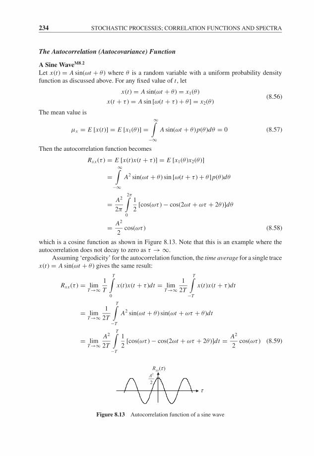
JWBK207-08 JWBK207-Shin January 18, 2008 10:6 Char Count= 0
234 STOCHASTIC PROCESSES; CORRELATION FUNCTIONS AND SPECTRA
The Autocorrelation (Autocovariance) Function
A Sine WaveM8.2
Let x(t) = A sin(ωt + θ ) where θ is a random variable with a uniform probability densityfunction as discussed above. For any fixed value of t , let
x(t) = A sin(ωt + θ ) = x1(θ )
x(t + τ ) = A sin [ω(t + τ ) + θ ] = x2(θ )(8.56)
The mean value is
μx = E [x(t)] = E [x1(θ )] =∞∫
−∞A sin(ωt + θ )p(θ )dθ = 0 (8.57)
Then the autocorrelation function becomes
Rxx (τ ) = E [x(t)x(t + τ )] = E [x1(θ )x2(θ )]
=∞∫
−∞A2 sin(ωt + θ ) sin [ω(t + τ ) + θ ]p(θ )dθ
= A2
2π
2π∫0
1
2[cos(ωτ ) − cos(2ωt + ωτ + 2θ )]dθ
= A2
2cos(ωτ ) (8.58)
which is a cosine function as shown in Figure 8.13. Note that this is an example where theautocorrelation does not decay to zero as τ → ∞.
Assuming ‘ergodicity’ for the autocorrelation function, the time average for a single tracex(t) = A sin(ωt + θ ) gives the same result:
Rxx (τ ) = limT →∞
1
T
T∫0
x(t)x(t + τ )dt = limT →∞
1
2T
T∫−T
x(t)x(t + τ )dt
= limT →∞
1
2T
T∫−T
A2 sin(ωt + θ ) sin(ωt + ωτ + θ )dt
= limT →∞
A2
2T
T∫−T
1
2[cos(ωτ ) − cos(2ωt + ωτ + 2θ )]dt = A2
2cos(ωτ ) (8.59)
2
2
A
( )xxR τ
τ
Figure 8.13 Autocorrelation function of a sine wave
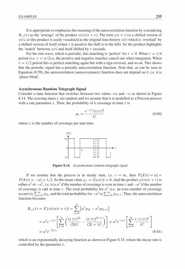
JWBK207-08 JWBK207-Shin January 18, 2008 10:6 Char Count= 0
EXAMPLES 235
It is appropriate to emphasize the meaning of the autocorrelation function by consideringRxx (τ ) as the ‘average’ of the product x(t)x(t + τ ). The term x(t + τ ) is a shifted version ofx(t), so this product is easily visualized as the original time history x(t) which is ‘overlaid’ bya shifted version of itself (when τ is positive the shift is to the left). So the product highlightsthe ‘match’ between x(t) and itself shifted by τ seconds.
For the sine wave, which is periodic, this matching is ‘perfect’ for τ = 0. When τ = 1/4period (i.e. τ = π/2ω), the positive and negative matches cancel out when integrated. Whenτ = 1/2 period this is perfect matching again but with a sign reversal, and so on. This showsthat the periodic signal has a periodic autocorrelation function. Note that, as can be seen inEquation (8.59), the autocorrelation (autocovariance) function does not depend on θ , i.e. it is‘phase blind’.
Asynchronous Random Telegraph SignalConsider a time function that switches between two values +a and −a as shown in Figure8.14. The crossing times ti are random and we assume that it is modelled as a Poisson processwith a rate parameter λ. Then, the probability of k crossings in time τ is
pk = e−λ|τ |(λ|τ |)k
k!(8.60)
where λ is the number of crossings per unit time.
( )x t
tit
a+
a−
Figure 8.14 Asynchronous random telegraph signal
If we assume that the process is in steady state, i.e. t → ∞, then P[X (t) = a] =P[X (t) = −a] = 1/2. So the mean value μx = E[x(t)] = 0. And the product x(t)x(t + τ ) iseither a2 or −a2, i.e. it is a2 if the number of crossings is even in time τ and −a2 if the numberof crossings is odd in time τ . The total probability for a2 (i.e. an even number of crossingsoccurs) is
∑∞k=0 p2k , and the total probability for −a2 is
∑∞k=0 p2k+1. Thus, the autocorrelation
function becomes
Rxx (τ ) = E [x(t)x(t + τ )] =∞∑
k=0
[a2 p2k − a2 p2k+1
]= a2e−λ|τ |
[ ∞∑k=0
((λ |τ |)2k
(2k)!− (λ |τ |)2k+1
(2k + 1)!
)]= a2e−λ|τ |
[ ∞∑k=0
(−λ |τ |)k
k!
]= a2e−2λ|τ | (8.61)
which is an exponentially decaying function as shown in Figure 8.15, where the decay rate iscontrolled by the parameter λ.

JWBK207-08 JWBK207-Shin January 18, 2008 10:6 Char Count= 0
236 STOCHASTIC PROCESSES; CORRELATION FUNCTIONS AND SPECTRA
2a
( )xxR τ
τ
Figure 8.15 Autocorrelation function of an asynchronous random telegraph signal
White NoiseThis is a very useful theoretical concept that has many desirable features in signal pro-cessing. In the previous example of the Poisson process, the autocorrelation function isdefined as Rxx (τ ) = a2e−2λ|τ |. Note that, as the parameter λ gets larger (i.e. the numberof crossings per unit time increases), Rxx (τ ) becomes narrower. We may relate this tothe concept of white noise by considering a limiting form. As λ → ∞, the process isvery erratic and Rxx (τ ) becomes ‘spike-like’. In order that Rxx (τ ) does not ‘disappearcompletely’ we can allow the value a to become large in compensation. This gives anidea of a ‘completely erratic’ random process whose autocorrelation (autocovariance)function is like a delta function, and the process that has this property is called whitenoise, i.e.
Autocorrelation function of white noise: Rxx (τ ) = kδ(τ ) (8.62)
An example of the autocorrelation function of white noise is shown in MATLABExample 8.10 which demonstrates some important aspects of correlation analysis relatedto system identification. Note, however, that in continuous time such processes cannotoccur in practice, and can only be approximated. Thus, we often refer to ‘band-limitedwhite noise’ whose spectral density function is constant within a band as we shall see inSection 8.7.
Synchronous Random Telegraph SignalConsider a switching signal where now the signal can only change sign at ‘event points’ spaced� seconds apart. At each event point the signal may switch or not (with equal probability) asshown in Figure 8.16.
t
( )x t
a+
a−Δ
Figure 8.16 Synchronous random telegraph signal
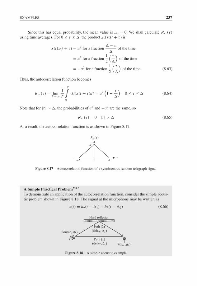
JWBK207-08 JWBK207-Shin January 18, 2008 10:6 Char Count= 0
EXAMPLES 237
Since this has equal probability, the mean value is μx = 0. We shall calculate Rxx (τ )using time averages. For 0 ≤ τ ≤ �, the product x(t)x(t + τ ) is
x(t)x(t + τ ) = a2 for a fraction� − τ
�of the time
= a2 for a fraction1
2
( τ
�
)of the time
= −a2 for a fraction1
2
( τ
�
)of the time (8.63)
Thus, the autocorrelation function becomes
Rxx (τ ) = limT →∞
1
T
T∫0
x(t)x(t + τ )dt = a2(
1 − τ
�
)0 ≤ τ ≤ � (8.64)
Note that for |τ | > �, the probabilities of a2 and −a2 are the same, so
Rxx (τ ) = 0 |τ | > � (8.65)
As a result, the autocorrelation function is as shown in Figure 8.17.
2a
( )xxR τ
Δ−Δτ
Figure 8.17 Autocorrelation function of a synchronous random telegraph signal
A Simple Practical ProblemM8.3
To demonstrate an application of the autocorrelation function, consider the simple acous-tic problem shown in Figure 8.18. The signal at the microphone may be written as
x(t) = as(t − �1) + bs(t − �2) (8.66)
Mic. x(t)
Hard reflector
1
Path (1)(delay, )Δ
2
Path (2)(delay, )ΔSource, ( )s t
Figure 8.18 A simple acoustic example
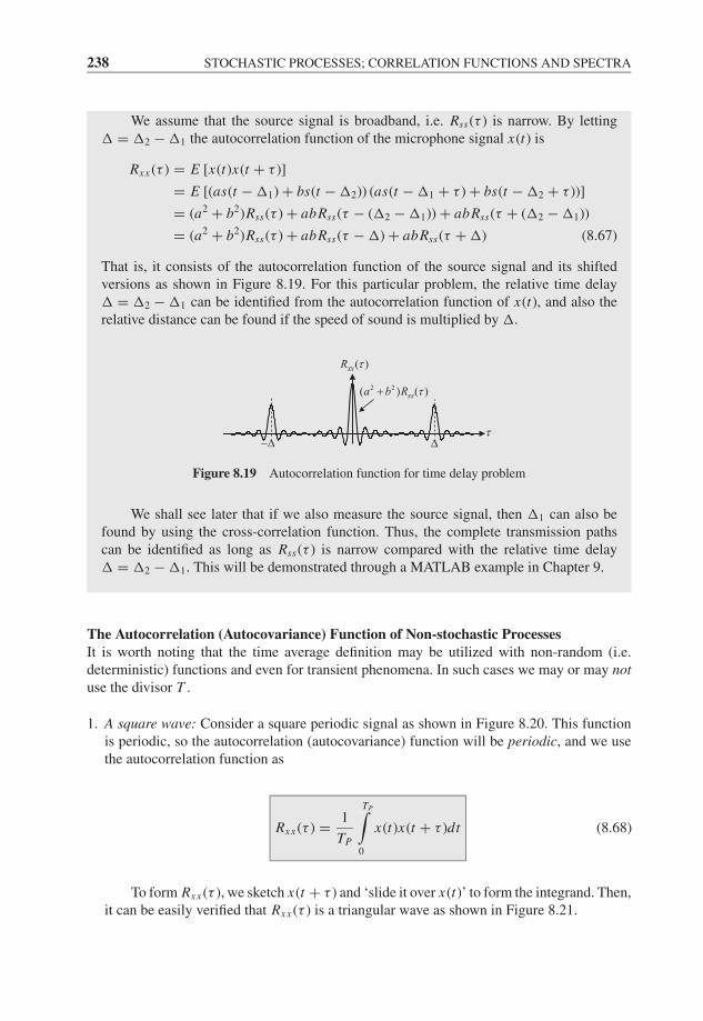
JWBK207-08 JWBK207-Shin January 18, 2008 10:6 Char Count= 0
238 STOCHASTIC PROCESSES; CORRELATION FUNCTIONS AND SPECTRA
We assume that the source signal is broadband, i.e. Rss(τ ) is narrow. By letting� = �2 − �1 the autocorrelation function of the microphone signal x(t) is
Rxx (τ ) = E [x(t)x(t + τ )]
= E [(as(t − �1) + bs(t − �2)) (as(t − �1 + τ ) + bs(t − �2 + τ ))]
= (a2 + b2)Rss(τ ) + abRss(τ − (�2 − �1)) + abRss(τ + (�2 − �1))
= (a2 + b2)Rss(τ ) + abRss(τ − �) + abRss(τ + �) (8.67)
That is, it consists of the autocorrelation function of the source signal and its shiftedversions as shown in Figure 8.19. For this particular problem, the relative time delay� = �2 − �1 can be identified from the autocorrelation function of x(t), and also therelative distance can be found if the speed of sound is multiplied by �.
( )xxR τ
−Δ Δ
2 2( ) ( )ssa b R τ+
τ
Figure 8.19 Autocorrelation function for time delay problem
We shall see later that if we also measure the source signal, then �1 can also befound by using the cross-correlation function. Thus, the complete transmission pathscan be identified as long as Rss(τ ) is narrow compared with the relative time delay� = �2 − �1. This will be demonstrated through a MATLAB example in Chapter 9.
The Autocorrelation (Autocovariance) Function of Non-stochastic ProcessesIt is worth noting that the time average definition may be utilized with non-random (i.e.deterministic) functions and even for transient phenomena. In such cases we may or may notuse the divisor T .
1. A square wave: Consider a square periodic signal as shown in Figure 8.20. This functionis periodic, so the autocorrelation (autocovariance) function will be periodic, and we usethe autocorrelation function as
Rxx (τ ) = 1
TP
TP∫0
x(t)x(t + τ )dt (8.68)
To form Rxx (τ ), we sketch x(t + τ ) and ‘slide it over x(t)’ to form the integrand. Then,it can be easily verified that Rxx (τ ) is a triangular wave as shown in Figure 8.21.
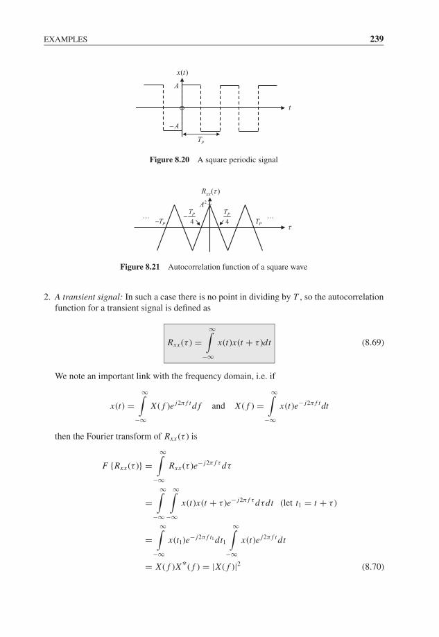
JWBK207-08 JWBK207-Shin January 18, 2008 10:6 Char Count= 0
EXAMPLES 239
( )x t
A
t
PT
A−
Figure 8.20 A square periodic signal
2A
( )xxR τ
4PT
PTPT− 4PT
− ......
τ
Figure 8.21 Autocorrelation function of a square wave
2. A transient signal: In such a case there is no point in dividing by T , so the autocorrelationfunction for a transient signal is defined as
Rxx (τ ) =∞∫
−∞x(t)x(t + τ )dt (8.69)
We note an important link with the frequency domain, i.e. if
x(t) =∞∫
−∞X ( f )e j2π f t d f and X ( f ) =
∞∫−∞
x(t)e− j2π f t dt
then the Fourier transform of Rxx (τ ) is
F {Rxx (τ )} =∞∫
−∞Rxx (τ )e− j2π f τ dτ
=∞∫
−∞
∞∫−∞
x(t)x(t + τ )e− j2π f τ dτdt (let t1 = t + τ )
=∞∫
−∞x(t1)e− j2π f t1 dt1
∞∫−∞
x(t)e j2π f t dt
= X ( f )X*( f ) = |X ( f )|2 (8.70)
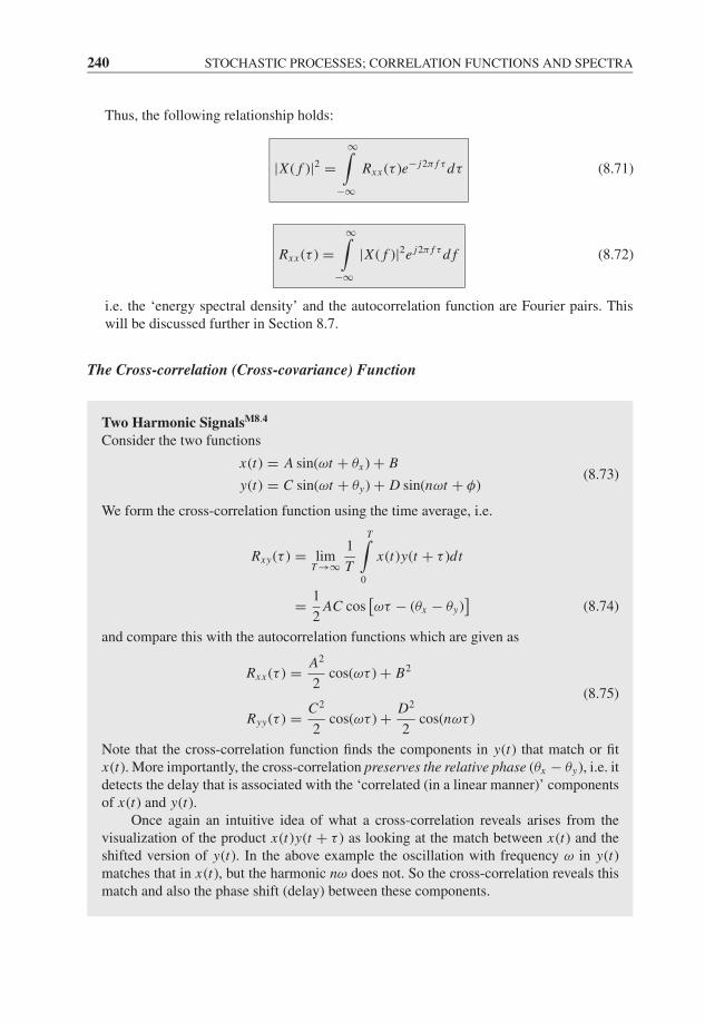
JWBK207-08 JWBK207-Shin January 18, 2008 10:6 Char Count= 0
240 STOCHASTIC PROCESSES; CORRELATION FUNCTIONS AND SPECTRA
Thus, the following relationship holds:
|X ( f )|2 =∞∫
−∞Rxx (τ )e− j2π f τ dτ (8.71)
Rxx (τ ) =∞∫
−∞|X ( f )|2e j2π f τ d f (8.72)
i.e. the ‘energy spectral density’ and the autocorrelation function are Fourier pairs. Thiswill be discussed further in Section 8.7.
The Cross-correlation (Cross-covariance) Function
Two Harmonic SignalsM8.4
Consider the two functions
x(t) = A sin(ωt + θx ) + B
y(t) = C sin(ωt + θy) + D sin(nωt + φ)(8.73)
We form the cross-correlation function using the time average, i.e.
Rxy(τ ) = limT →∞
1
T
T∫0
x(t)y(t + τ )dt
= 1
2AC cos
[ωτ − (θx − θy)
](8.74)
and compare this with the autocorrelation functions which are given as
Rxx (τ ) = A2
2cos(ωτ ) + B2
Ryy(τ ) = C2
2cos(ωτ ) + D2
2cos(nωτ )
(8.75)
Note that the cross-correlation function finds the components in y(t) that match or fitx(t). More importantly, the cross-correlation preserves the relative phase (θx − θy), i.e. itdetects the delay that is associated with the ‘correlated (in a linear manner)’ componentsof x(t) and y(t).
Once again an intuitive idea of what a cross-correlation reveals arises from thevisualization of the product x(t)y(t + τ ) as looking at the match between x(t) and theshifted version of y(t). In the above example the oscillation with frequency ω in y(t)matches that in x(t), but the harmonic nω does not. So the cross-correlation reveals thismatch and also the phase shift (delay) between these components.
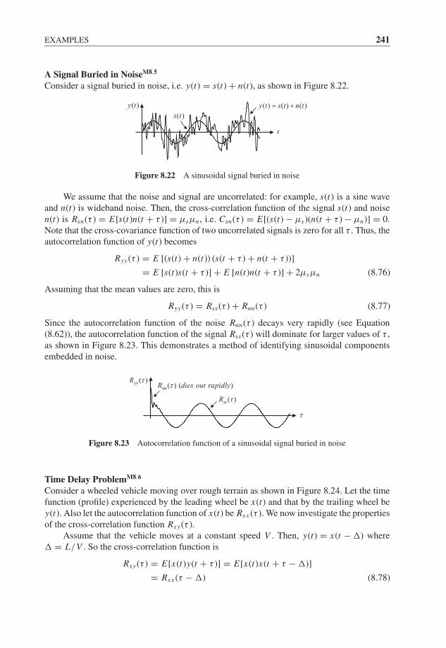
JWBK207-08 JWBK207-Shin January 18, 2008 10:6 Char Count= 0
EXAMPLES 241
A Signal Buried in NoiseM8.5
Consider a signal buried in noise, i.e. y(t) = s(t) + n(t), as shown in Figure 8.22.
( ) ( ) ( )y t s t n t= +( )s t
( )y t
t
Figure 8.22 A sinusoidal signal buried in noise
We assume that the noise and signal are uncorrelated: for example, s(t) is a sine waveand n(t) is wideband noise. Then, the cross-correlation function of the signal s(t) and noisen(t) is Rsn(τ ) = E[s(t)n(t + τ )] = μsμn , i.e. Csn(τ ) = E[(s(t) − μs)(n(t + τ ) − μn)] = 0.Note that the cross-covariance function of two uncorrelated signals is zero for all τ . Thus, theautocorrelation function of y(t) becomes
Ryy(τ ) = E [(s(t) + n(t)) (s(t + τ ) + n(t + τ ))]
= E [s(t)s(t + τ )] + E [n(t)n(t + τ )] + 2μsμn (8.76)
Assuming that the mean values are zero, this is
Ryy(τ ) = Rss(τ ) + Rnn(τ ) (8.77)
Since the autocorrelation function of the noise Rnn(τ ) decays very rapidly (see Equation(8.62)), the autocorrelation function of the signal Rss(τ ) will dominate for larger values of τ ,as shown in Figure 8.23. This demonstrates a method of identifying sinusoidal componentsembedded in noise.
( )yyR τ( ) ( )nnR dies out rapidlyτ
( )ssR τ
τ
Figure 8.23 Autocorrelation function of a sinusoidal signal buried in noise
Time Delay ProblemM8.6
Consider a wheeled vehicle moving over rough terrain as shown in Figure 8.24. Let the timefunction (profile) experienced by the leading wheel be x(t) and that by the trailing wheel bey(t). Also let the autocorrelation function of x(t) be Rxx (τ ). We now investigate the propertiesof the cross-correlation function Rxy(τ ).
Assume that the vehicle moves at a constant speed V . Then, y(t) = x(t − �) where� = L/V . So the cross-correlation function is
Rxy(τ ) = E[x(t)y(t + τ )] = E[x(t)x(t + τ − �)]
= Rxx (τ − �) (8.78)
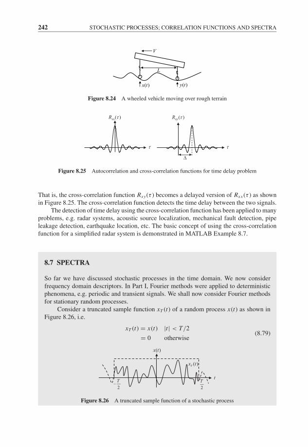
JWBK207-08 JWBK207-Shin January 18, 2008 10:6 Char Count= 0
242 STOCHASTIC PROCESSES; CORRELATION FUNCTIONS AND SPECTRA
( )x t ( )y t
L
V
Figure 8.24 A wheeled vehicle moving over rough terrain
( )xyR τ
Δ
τ
( )xxR τ
τ
Figure 8.25 Autocorrelation and cross-correlation functions for time delay problem
That is, the cross-correlation function Rxy(τ ) becomes a delayed version of Rxx (τ ) as shownin Figure 8.25. The cross-correlation function detects the time delay between the two signals.
The detection of time delay using the cross-correlation function has been applied to manyproblems, e.g. radar systems, acoustic source localization, mechanical fault detection, pipeleakage detection, earthquake location, etc. The basic concept of using the cross-correlationfunction for a simplified radar system is demonstrated in MATLAB Example 8.7.
8.7 SPECTRA
So far we have discussed stochastic processes in the time domain. We now considerfrequency domain descriptors. In Part I, Fourier methods were applied to deterministicphenomena, e.g. periodic and transient signals. We shall now consider Fourier methodsfor stationary random processes.
Consider a truncated sample function xT (t) of a random process x(t) as shown inFigure 8.26, i.e.
xT (t) = x(t) |t | < T/2
= 0 otherwise(8.79)
2
T−
2
Tt
( )x t
( )Tx t
Figure 8.26 A truncated sample function of a stochastic process

JWBK207-08 JWBK207-Shin January 18, 2008 10:6 Char Count= 0
SPECTRA 243
We shall consider the decomposition of the power of this sample function in thefrequency domain. As seen from the figure, the truncated signal xT (t) is pulse-like, i.e. itcan be regarded as a transient signal. Thus, it can be represented by the Fourier integral
xT (t) =∞∫
−∞XT ( f )e j2π f t d f (8.80)
Since the total energy of the signal∫ ∞−∞ x2
T (t)dt tends to infinity as T gets large, we shallconsider the average power of the signal, i.e.
1
T
∞∫−∞
x2T (t)dt
Then, by Parseval’s theorem it can be shown that
1
T
∞∫−∞
x2T (t)dt = 1
T
T/2∫−T/2
x2T (t)dt = 1
T
∞∫−∞
|XT ( f )|2d f =∞∫
−∞
1
T|XT ( f )|2d f (8.81)
where the quantity |XT ( f )|2/T is called the raw (or sample) power spectral density,which is denoted as
Sxx ( f ) = 1
T|XT ( f )|2 (8.82)
Note that the power of the signal in a data segment of length T is
1
T
∞∫−∞
x2T (t)dt =
∞∫−∞
Sxx ( f )d f (8.83)
Now, as T → ∞ Equation (8.81) can be written as
limT →∞
1
T
T/2∫−T/2
x2T (t)dt =
∞∫−∞
limT →∞
|XT ( f )|2T
d f (8.84)
Note that the left hand side of the equation is the average power of the sample function,thus it may be tempting to define limT →∞|XT ( f )|2/T as the power spectral density.However we shall see (later) that Sxx ( f ) does not converge (in a statistical sense) asT → ∞, which is the reason that the term ‘raw’ is used. In Chapter 10, we shall seethat Sxx ( f ) evaluated from a larger data length is just as erratic as for the shorter datalength, i.e. the estimate Sxx ( f ) cannot be improved simply by using more data (evenfor T → ∞). We shall also see later (in Chapter 10) that the standard deviation of theestimate is as great as the quantity being estimated! That is, it is independent of datalength and equal to the true spectral density as follows:
Var(Sxx ( f )
) = S2xx ( f )
(or
Var(Sxx ( f )
)S2
xx ( f )= 1
)(8.85)
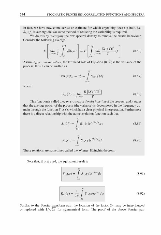
JWBK207-08 JWBK207-Shin January 18, 2008 10:6 Char Count= 0
244 STOCHASTIC PROCESSES; CORRELATION FUNCTIONS AND SPECTRA
In fact, we have now come across an estimate for which ergodicity does not hold, i.e.Sxx ( f ) is not ergodic. So some method of reducing the variability is required.
We do this by averaging the raw spectral density to remove the erratic behaviour.Consider the following average
E
⎡⎢⎣ limT →∞
1
T
T/2∫−T/2
x2T (t)dt
⎤⎥⎦ = E
⎡⎣ ∞∫−∞
limT →∞
|XT ( f )|2T
d f
⎤⎦ (8.86)
Assuming zero mean values, the left hand side of Equation (8.86) is the variance of theprocess, thus it can be written as
Var (x(t)) = σ 2x =
∞∫−∞
Sxx ( f )d f (8.87)
where
Sxx ( f ) = limT →∞
E[|XT ( f )|2]
T(8.88)
This function is called the power spectral density function of the process, and it statesthat the average power of the process (the variance) is decomposed in the frequency do-main through the function Sxx ( f ), which has a clear physical interpretation. Furthermorethere is a direct relationship with the autocorrelation function such that
Sxx ( f ) =∞∫
−∞Rxx (τ )e− j2π f τ dτ (8.89)
Rxx (τ ) =∞∫
−∞Sxx ( f )e j2π f τ d f (8.90)
These relations are sometimes called the Wiener–Khinchin theorem.
Note that, if ω is used, the equivalent result is
Sxx (ω) =∞∫
−∞Rxx (τ )e− jωτ dτ (8.91)
Rxx (τ ) = 1
2π
∞∫−∞
Sxx (ω)e jωτ dω (8.92)
Similar to the Fourier transform pair, the location of the factor 2π may be interchangedor replaced with 1/
√2π for symmetrical form. The proof of the above Fourier pair

JWBK207-08 JWBK207-Shin January 18, 2008 10:6 Char Count= 0
SPECTRA 245
(Equations (8.89)–(8.92)) needs some elements discussed in Chapter 10, so this will be justifiedlater.
Note that the function Sxx ( f ) is an even function of frequency and is sometimes calledthe two-sided power spectral density. If x(t) is in volts, Sxx ( f ) has units of volts2/Hz. Often aone-sided power spectral density is defined as
Gxx ( f ) = 2Sxx ( f ) f > 0
= Sxx ( f ) f = 0
= 0 f < 0
(8.93)
Examples of Power Spectral Density Functions1
(a) If Rxx (τ ) = kδ(τ ), k > 0, i.e. white noise, then
Sxx ( f ) =∞∫
−∞Rxx (τ )e− j2π f τ dτ =
∞∫−∞
kδ(τ )e− j2π f τ dτ = ke− j2π f ·0 = k (8.94)
τ
( )xxR τ
k
f
( )xxS f
k
Figure 8.27 Power spectral density of white noise
Note that a ‘narrow’ autocorrelation function results in a broadband spectrum (Figure 8.27).
(b) If Rxx (τ ) = σ 2x e−λ|τ |, λ > 0, then
Sxx ( f ) =∞∫
−∞Rxx (τ )e− j2π f τ dτ =
∞∫−∞
σ 2x e−λ|τ |e− j2π f τ dτ
= σ 2x
⎡⎣ 0∫−∞
eλτ e− j2π f τ dτ +∞∫
0
e−λτ e− j2π f τ dτ
⎤⎦ = 2λσ 2x
λ2 + (2π f )2(8.95)
( )xxS f22 xσ
λ
f
2
xσ
( )xxR τ
τ
Figure 8.28 Exponentially decaying autocorrelation and corresponding power spectral density
The exponentially decaying autocorrelation function results in a mainly low-frequencypower spectral density function (Figure 8.28).
1 See examples in Section 4.3 and compare.
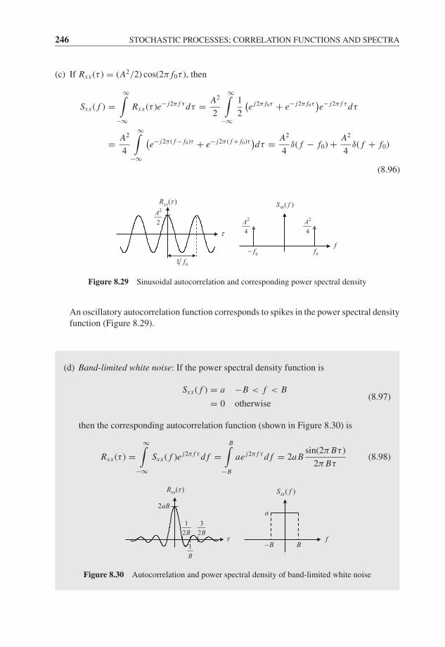
JWBK207-08 JWBK207-Shin January 18, 2008 10:6 Char Count= 0
246 STOCHASTIC PROCESSES; CORRELATION FUNCTIONS AND SPECTRA
(c) If Rxx (τ ) = (A2/2) cos(2π f0τ ), then
Sxx ( f ) =∞∫
−∞Rxx (τ )e− j2π f τ dτ = A2
2
∞∫−∞
1
2
(e j2π f0τ + e− j2π f0τ
)e− j2π f τ dτ
= A2
4
∞∫−∞
(e− j2π ( f − f0)τ + e− j2π ( f + f0)τ
)dτ = A2
4δ( f − f0) + A2
4δ( f + f0)
(8.96)
( )xxR τ
01 f
2
2
A
τ
( )xxS f
0f− 0f
2
4
A
f
2
4
A
Figure 8.29 Sinusoidal autocorrelation and corresponding power spectral density
An oscillatory autocorrelation function corresponds to spikes in the power spectral densityfunction (Figure 8.29).
(d) Band-limited white noise: If the power spectral density function is
Sxx ( f ) = a −B < f < B
= 0 otherwise(8.97)
then the corresponding autocorrelation function (shown in Figure 8.30) is
Rxx (τ ) =∞∫
−∞Sxx ( f )e j2π f τ d f =
B∫−B
ae j2π f τ d f = 2aBsin(2π Bτ )
2π Bτ(8.98)
1
B
1
2B
3
2B
( )xxR τ
τ
2aB
( )xxS f
f
a
B− B
Figure 8.30 Autocorrelation and power spectral density of band-limited white noise

JWBK207-08 JWBK207-Shin January 18, 2008 10:6 Char Count= 0
SPECTRA 247
The Cross-spectral Density Function
Generalizing the Wiener–Khinchin theorem, the cross-spectral density function is‘defined’ as
Sxy( f ) =∞∫
−∞Rxy(τ )e− j2π f τ dτ (8.99)
with inverse
Rxy(τ ) =∞∫
−∞Sxy( f )e j2π f τ d f (8.100)
As with the power spectral density function, if ω is used in place of f , then
Sxy(ω) =∞∫
−∞Rxy(τ )e− jωτ dτ (8.101)
Rxy(τ ) = 1
2π
∞∫−∞
Sxy(ω)e jωτ dω (8.102)
Alternatively, Sxy( f ) is defined as
Sxy( f ) = limT →∞
E[X*T ( f )YT ( f )]
T(8.103)
where XT ( f ) and YT ( f ) are Fourier transforms of truncated functions xT (t) and yT (t)defined for | t | < T/2 (see Figure 8.26).
The equivalence of Equations (8.99) and (8.103) may be justified in the same manneras for the power spectral density functions as discussed in Chapter 10.
In general, the cross-spectral density function is complex valued, i.e.
Sxy( f ) = ∣∣Sxy( f )∣∣ e j arg Sxy ( f ) (8.104)
This can be interpreted as the frequency domain equivalent of the cross-correlation func-tion. That is, |Sxy( f )| is the cross-amplitude spectrum and it shows whether frequencycomponents in one signal are ‘associated’ with large or small amplitude at the samefrequency in the other signal, i.e. it is the measure of association of amplitude in x andy at frequency f ; arg Sxy( f ) is the phase spectrum and this shows whether frequencycomponents in one signal ‘lag’ or ‘lead’ the components at the same frequency in theother signal, i.e. it shows lags/leads (or phase difference) between x and y at frequency f .
Properties of the Cross-spectral Density Function
(a) An important property is
Sxy( f ) = S*yx ( f ) (8.105)
This can be easily proved using the fact that Rxy(τ ) = Ryx (−τ ).
JWBK207-08 JWBK207-Shin January 18, 2008 10:6 Char Count= 0
248 STOCHASTIC PROCESSES; CORRELATION FUNCTIONS AND SPECTRA
(b) A one-sided cross-spectral density function Gxy( f ) is defined as
Gxy( f ) = 2Sxy( f ) f > 0
= Sxy( f ) f = 0
= 0 f < 0
(8.106)
(c) The coincident spectral density (co-spectrum) and quadrature spectral density (quad-spectrum) are defined as (Bendat and Piersol, 2000)
Gxy( f ) = 2
∞∫−∞
Rxy(τ )e− j2π f τ dτ = Cxy( f ) − j Qxy( f ) f ≥ 0 (8.107)
where Cxy( f ) and Qxy( f ) are called the co-spectra and quad-spectra, respectively (thereason for these names is explained later in the example given in page 249). Cxy( f ) is aneven function of f and Qxy( f ) is an odd function of f . Also, by writing Rxy(τ ) as thesum of even and odd parts (see Equation (3.18)), then
Cxy( f ) = 2
∞∫0
[Rxy(τ ) + Ryx (τ )
]cos(2π f τ )dτ = Cxy(− f ) (8.108)
Qxy( f ) = 2
∞∫0
[Rxy(τ ) − Ryx (τ )
]sin(2π f τ )dτ = −Qxy(− f ) (8.109)
Similar to Sxy( f ), the one-sided cross-spectral density function Gxy( f ) can bewritten as
Gxy( f ) = ∣∣Gxy( f )∣∣ e j arg Gxy ( f ) (8.110)
Then, it can be shown that ∣∣Gxy( f )∣∣ =
√C2
xy( f ) + Q2xy( f ) (8.111)
and
arg Gxy( f ) = − tan−1
(Qxy( f )
Cxy( f )
)(8.112)
(d) For the phase of Sxy( f ) = ∣∣Sxy( f )∣∣ e j arg Sxy ( f ), let θx ( f ) and θy( f ) be the phase com-
ponents at frequency f corresponding to x(t) and y(t), respectively. Then, arg Sxy( f )gives the phase difference such that
arg Sxy( f ) = − [θx ( f ) − θy( f )
](8.113)
JWBK207-08 JWBK207-Shin January 18, 2008 10:6 Char Count= 0
SPECTRA 249
which is θy( f ) − θx ( f ). Note that it is not θx ( f ) − θy( f ) (see Equation (8.103) where
X*T ( f ) is multiplied by YT ( f ), and also compare it with Equations (8.73) and (8.74)).
Thus, in some texts, Sxy( f ) is defined as
Sxy( f ) = ∣∣Sxy( f )∣∣ e− jθxy ( f ) (8.114)
where θxy( f ) = θx ( f ) − θy( f ). So, care must be taken with the definitions.
(e) A useful inequality satisfied by Sxy( f ) is∣∣Sxy( f )∣∣2 ≤ Sxx ( f )Syy( f ) (8.115)
or ∣∣Gxy( f )∣∣2 ≤ Gxx ( f )G yy( f ) (8.116)
The proof of this result is given in Appendix B. We shall see later that this is a par-ticularly useful result – we shall define, in Chapter 9, the ‘coherence function’ as∣∣Sxy( f )
∣∣2/(Sxx ( f )Syy( f )) which is a normalized cross-spectral density function.
Examples of Cross-spectral Density Functions
Two examples are as follows:
(a) Consider two functions (see also Equation (8.73) in Section 8.6)M8.8
x(t) = A sin(2πpt + θx )
y(t) = C sin(2πpt + θy) + D sin(n2πpt + φ)(8.117)
In the previous section, it was shown that the cross-correlation function is
Rxy(τ ) = 1
2AC cos
[2πpτ − (θx − θy)
](8.118)
Let θxy = θx − θy ; then
Rxy(τ ) = 1
2AC cos(2πpτ − θxy) (8.119)
The cross-spectral density function is
Sxy( f ) =∞∫
−∞Rxy(τ )e− j2π f τ dτ = AC
4
∞∫−∞
(e j(2πpτ−θxy) + e− j(2πpτ−θxy)
)e− j2π f τ dτ
= AC
4
∞∫−∞
(e− j2π ( f −p)τ e− jθxy + e− j2π ( f +p)τ e jθxy
)dτ
= AC
4
[δ( f − p)e− jθxy + δ( f + p)e jθxy
](8.120)
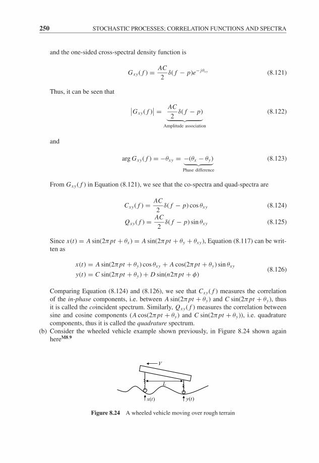
JWBK207-08 JWBK207-Shin January 18, 2008 10:6 Char Count= 0
250 STOCHASTIC PROCESSES; CORRELATION FUNCTIONS AND SPECTRA
and the one-sided cross-spectral density function is
Gxy( f ) = AC
2δ( f − p)e− jθxy (8.121)
Thus, it can be seen that
∣∣Gxy( f )∣∣ = AC
2δ( f − p)︸ ︷︷ ︸
Amplitude association
(8.122)
and
arg Gxy( f ) = −θxy = −(θx − θy)︸ ︷︷ ︸Phase difference
(8.123)
From Gxy( f ) in Equation (8.121), we see that the co-spectra and quad-spectra are
Cxy( f ) = AC
2δ( f − p) cos θxy (8.124)
Qxy( f ) = AC
2δ( f − p) sin θxy (8.125)
Since x(t) = A sin(2πpt + θx ) = A sin(2πpt + θy + θxy), Equation (8.117) can be writ-ten as
x(t) = A sin(2πpt + θy) cos θxy + A cos(2πpt + θy) sin θxy
y(t) = C sin(2πpt + θy) + D sin(n2πpt + φ)(8.126)
Comparing Equation (8.124) and (8.126), we see that Cxy( f ) measures the correlationof the in-phase components, i.e. between A sin(2πpt + θy) and C sin(2πpt + θy), thusit is called the coincident spectrum. Similarly, Qxy( f ) measures the correlation betweensine and cosine components (A cos(2πpt + θy) and C sin(2πpt + θy)), i.e. quadraturecomponents, thus it is called the quadrature spectrum.
(b) Consider the wheeled vehicle example shown previously, in Figure 8.24 shown againhereM8.9
( )x t ( )y t
L
V
Figure 8.24 A wheeled vehicle moving over rough terrain
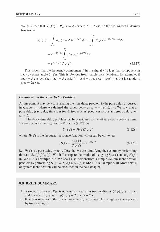
JWBK207-08 JWBK207-Shin January 18, 2008 10:6 Char Count= 0
BRIEF SUMMARY 251
We have seen that Rxy(τ ) = Rxx (τ − �), where � = L/V . So the cross-spectral densityfunction is
Sxy( f ) =∞∫
−∞Rxx (τ − �)e− j2π f τ dτ =
∞∫−∞
Rxx (u)e− j2π f (u+�)du
= e− j2π f �
∞∫−∞
Rxx (u)e− j2π f udu
= e− j2π f �Sxx ( f ) (8.127)
This shows that the frequency component f in the signal y(t) lags that component inx(t) by phase angle 2π f �. This is obvious from simple considerations: for example, ifx(t) = A cos(ωt) then y(t) = A cos [ω(t − �)] = A cos(ωt − ω�), i.e. the lag angle isω� = 2π f �.
Comments on the Time Delay Problem
At this point, it may be worth relating the time delay problem to the pure delay discussedin Chapter 4, where we defined the group delay as tg = −dφ(ω)/dω. We saw that apure delay (say, delay time is � for all frequencies) produces a constant group delay, i.e.tg = �.
The above time delay problem can be considered as identifying a pure delay system.To see this more clearly, rewrite Equation (8.127) as
Sxy( f ) = H ( f )Sxx ( f ) (8.128)
where H ( f ) is the frequency response function which can be written as
H ( f ) = Sxy( f )
Sxx ( f )= e− j2π f � (8.129)
i.e. H ( f ) is a pure delay system. Note that we are identifying the system by performingthe ratio Sxy( f )/Sxx ( f ). We shall compare the results of using arg Sxy( f ) and arg H ( f )in MATLAB Example 8.9. We shall also demonstrate a simple system identificationproblem by performing H ( f ) = Sxy( f )/Sxx ( f ) in MATLAB Example 8.10. More detailsof system identification will be discussed in the next chapter.
8.8 BRIEF SUMMARY
1. A stochastic process X (t) is stationary if it satisfies two conditions: (i) p(x, t) = p(x)and (ii) p(x1, t1; x2, t2) = p(x1, t1 + T ; x2, t2 + T ).
2. If certain averages of the process are ergodic, then ensemble averages can be replacedby time averages.
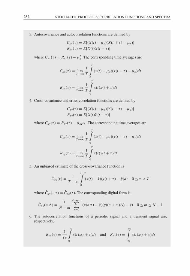
JWBK207-08 JWBK207-Shin January 18, 2008 10:6 Char Count= 0
252 STOCHASTIC PROCESSES; CORRELATION FUNCTIONS AND SPECTRA
3. Autocovariance and autocorrelation functions are defined by
Cxx (τ ) = E[(X (t) − μx )(X (t + τ ) − μx )]
Rxx (τ ) = E[X (t)X (t + τ )]
where Cxx (τ ) = Rxx (τ ) − μ2x . The corresponding time averages are
Cxx (τ ) = limT →∞
1
T
T∫0
(x(t) − μx )(x(t + τ ) − μx )dt
Rxx (τ ) = limT →∞
1
T
T∫0
x(t)x(t + τ )dt
4. Cross-covariance and cross-correlation functions are defined by
Cxy(τ ) = E[(X (t) − μx )(Y (t + τ ) − μy)]
Rxy(τ ) = E[X (t)Y (t + τ )]
where Cxy(τ ) = Rxy(τ ) − μxμy . The corresponding time averages are
Cxy(τ ) = limT →∞
1
T
T∫0
(x(t) − μx )(y(t + τ ) − μy)dt
Rxy(τ ) = limT →∞
1
T
T∫0
x(t)y(t + τ )dt
5. An unbiased estimate of the cross-covariance function is
Cxy(τ ) = 1
T − τ
T −τ∫0
(x(t) − x)(y(t + τ ) − y)dt 0 ≤ τ < T
where Cxy(−τ ) = Cyx (τ ). The corresponding digital form is
Cxy(m�) = 1
N − m
N−m−1∑n=0
(x(n�) − x)(y((n + m)�) − y) 0 ≤ m ≤ N − 1
6. The autocorrelation functions of a periodic signal and a transient signal are,respectively,
Rxx (τ ) = 1
TP
TP∫0
x(t)x(t + τ )dt and Rxx (τ ) =∞∫
−∞x(t)x(t + τ )dt

JWBK207-08 JWBK207-Shin January 18, 2008 10:6 Char Count= 0
MATLAB EXAMPLES 253
7. The autocorrelation function of white noise is
Rxx (τ ) = kδ(τ )
8. The cross-correlation function of two uncorrelated signals s(t) and n(t) is
Rsn(τ ) = E [s(t)n(t + τ )] = 0 (assuming zero mean values)
9. The power spectral density and cross-spectral density functions are
Sxx ( f ) = limT →∞
E[|XT ( f )|2]
Tand Sxy( f ) = lim
T →∞
E[
X*T ( f )YT ( f )
]T
and the corresponding raw (or sample) spectral density functions are
Sxx ( f ) = 1
T|XT ( f )|2 and Sxy( f ) = 1
TX*
T ( f )YT ( f )
10. The Wiener–Khinchin theorem is
Sxx ( f ) =∞∫
−∞Rxx (τ )e− j2π f τ dτ and Rxx (τ ) =
∞∫−∞
Sxx ( f )e j2π f τ d f
Also,
Sxy( f ) =∞∫
−∞Rxy(τ )e− j2π f τ dτ and Rxy(τ ) =
∞∫−∞
Sxy( f )e j2π f τ d f
11. The cross-spectral density function is complex valued, i.e.
Sxy( f ) = ∣∣Sxy( f )∣∣ e j arg Sxy ( f ) and Sxy( f ) = S*
yx ( f )
where |Sxy( f )| is the measure of association of amplitude in x and y at frequency f ,and arg Sxy( f ) shows lags/leads (or phase difference) between x and y at frequency f .
8.9 MATLAB EXAMPLES
Example 8.1: Probability density function of a sine wave
The theoretical probability density function of a sine wave x(t) = A sin(ωt + θ ) is
p(x) = 1
π√
A2 − x2
In this MATLAB example, we compare the histograms resulting from the ensembleaverage and the time average. For the ensemble average θ is a random variable and t isfixed, and for the time average θ is fixed and t is a time variable.
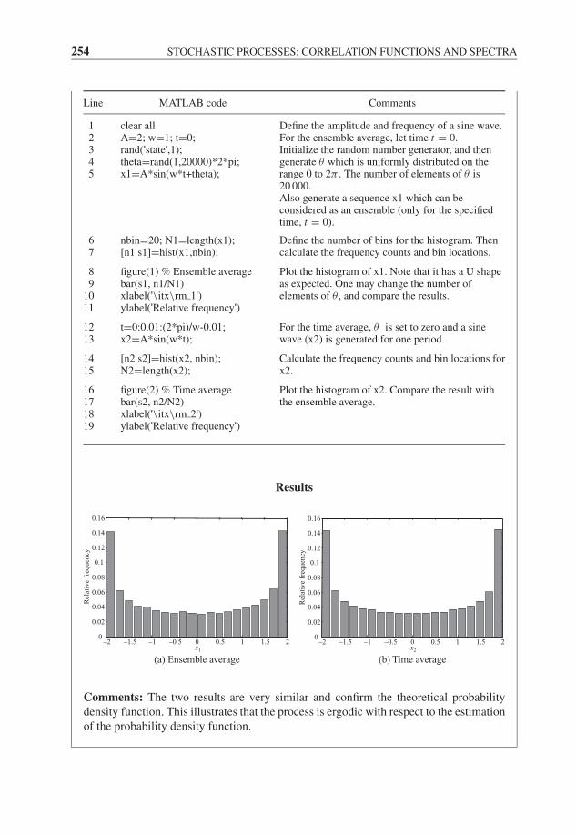
JWBK207-08 JWBK207-Shin January 18, 2008 10:6 Char Count= 0
254 STOCHASTIC PROCESSES; CORRELATION FUNCTIONS AND SPECTRA
Line MATLAB code Comments
12345
clear allA=2; w=1; t=0;rand('state',1);theta=rand(1,20000)*2*pi;x1=A*sin(w*t+theta);
Define the amplitude and frequency of a sine wave.For the ensemble average, let time t = 0.Initialize the random number generator, and thengenerate θ which is uniformly distributed on therange 0 to 2π . The number of elements of θ is20 000.Also generate a sequence x1 which can beconsidered as an ensemble (only for the specifiedtime, t = 0).
67
nbin=20; N1=length(x1);[n1 s1]=hist(x1,nbin);
Define the number of bins for the histogram. Thencalculate the frequency counts and bin locations.
89
1011
figure(1) % Ensemble averagebar(s1, n1/N1)xlabel('\itx\rm 1')ylabel('Relative frequency')
Plot the histogram of x1. Note that it has a U shapeas expected. One may change the number ofelements of θ , and compare the results.
1213
t=0:0.01:(2*pi)/w-0.01;x2=A*sin(w*t);
For the time average, θ is set to zero and a sinewave (x2) is generated for one period.
1415
[n2 s2]=hist(x2, nbin);N2=length(x2);
Calculate the frequency counts and bin locations forx2.
16171819
figure(2) % Time averagebar(s2, n2/N2)xlabel('\itx\rm 2')ylabel('Relative frequency')
Plot the histogram of x2. Compare the result withthe ensemble average.
Results
–2 –1.5 –1 –0.5 0 0.5 1 1.5 20
0.02
0.04
0.06
0.08
0.1
0.12
0.14
0.16
Rel
ativ
e fr
equen
cy
x1
–2 –1.5
(a) Ensemble average (b) Time average
–1 –0.5 0 0.5 1 1.5 20
0.02
0.04
0.06
0.08
0.1
0.12
0.14
0.16
Rel
ativ
e fr
equen
cy
x2
Comments: The two results are very similar and confirm the theoretical probabilitydensity function. This illustrates that the process is ergodic with respect to the estimationof the probability density function.
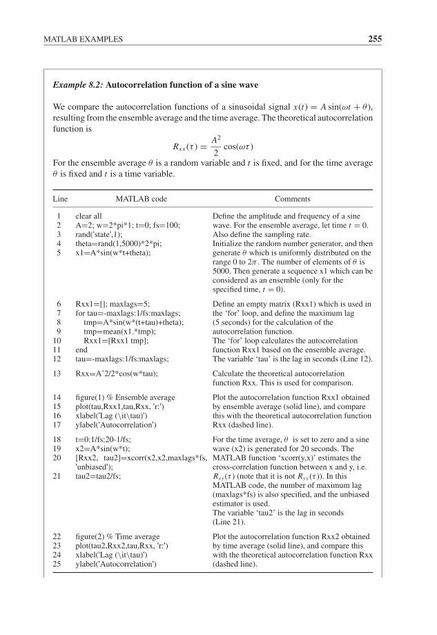
JWBK207-08 JWBK207-Shin January 18, 2008 10:6 Char Count= 0
MATLAB EXAMPLES 255
Example 8.2: Autocorrelation function of a sine wave
We compare the autocorrelation functions of a sinusoidal signal x(t) = A sin(ωt + θ ),resulting from the ensemble average and the time average. The theoretical autocorrelationfunction is
Rxx (τ ) = A2
2cos(ωτ )
For the ensemble average θ is a random variable and t is fixed, and for the time averageθ is fixed and t is a time variable.
Line MATLAB code Comments
12345
clear allA=2; w=2*pi*1; t=0; fs=100;rand('state',1);theta=rand(1,5000)*2*pi;x1=A*sin(w*t+theta);
Define the amplitude and frequency of a sinewave. For the ensemble average, let time t = 0.Also define the sampling rate.Initialize the random number generator, and thengenerate θ which is uniformly distributed on therange 0 to 2π . The number of elements of θ is5000. Then generate a sequence x1 which can beconsidered as an ensemble (only for thespecified time, t = 0).
6789
101112
Rxx1=[]; maxlags=5;for tau=-maxlags:1/fs:maxlags;
tmp=A*sin(w*(t+tau)+theta);tmp=mean(x1.*tmp);Rxx1=[Rxx1 tmp];
endtau=-maxlags:1/fs:maxlags;
Define an empty matrix (Rxx1) which is used inthe ‘for’ loop, and define the maximum lag(5 seconds) for the calculation of theautocorrelation function.The ‘for’ loop calculates the autocorrelationfunction Rxx1 based on the ensemble average.The variable ‘tau’ is the lag in seconds (Line 12).
13 Rxx=Aˆ2/2*cos(w*tau); Calculate the theoretical autocorrelationfunction Rxx. This is used for comparison.
14151617
figure(1) % Ensemble averageplot(tau,Rxx1,tau,Rxx, 'r:')xlabel('Lag (\it\tau)')ylabel('Autocorrelation')
Plot the autocorrelation function Rxx1 obtainedby ensemble average (solid line), and comparethis with the theoretical autocorrelation functionRxx (dashed line).
181920
21
t=0:1/fs:20-1/fs;x2=A*sin(w*t);[Rxx2, tau2]=xcorr(x2,x2,maxlags*fs,'unbiased');tau2=tau2/fs;
For the time average, θ is set to zero and a sinewave (x2) is generated for 20 seconds. TheMATLAB function ‘xcorr(y,x)’ estimates thecross-correlation function between x and y, i.e.Rxy(τ ) (note that it is not Ryx (τ )). In thisMATLAB code, the number of maximum lag(maxlags*fs) is also specified, and the unbiasedestimator is used.The variable ‘tau2’ is the lag in seconds(Line 21).
22232425
figure(2) % Time averageplot(tau2,Rxx2,tau,Rxx, 'r:')xlabel('Lag (\it\tau)')ylabel('Autocorrelation')
Plot the autocorrelation function Rxx2 obtainedby time average (solid line), and compare thiswith the theoretical autocorrelation function Rxx(dashed line).
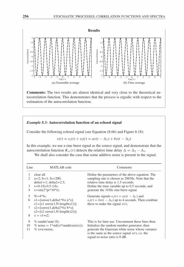
JWBK207-08 JWBK207-Shin January 18, 2008 10:6 Char Count= 0
256 STOCHASTIC PROCESSES; CORRELATION FUNCTIONS AND SPECTRA
Results
–5 –4 –3 –2 –1 0 1 2 3
(a) Ensemble average (b) Time average
4 5–2
–1.5
–1
–0.5
0
0.5
1
1.5
2
Lag (τ )
Auto
corr
elat
ion
–5 –4 –3 –2 –1 0 1 2 3 4 5–2
–1.5
–1
–0.5
0
0.5
1
1.5
2
Lag (τ )
Auto
corr
elat
ion
Comments: The two results are almost identical and very close to the theoretical au-tocorrelation function. This demonstrates that the process is ergodic with respect to theestimation of the autocorrelation function.
Example 8.3: Autocorrelation function of an echoed signal
Consider the following echoed signal (see Equation (8.66) and Figure 8.18):
x(t) = s1(t) + s2(t) = as(t − �1) + bs(t − �2)
In this example, we use a sine burst signal as the source signal, and demonstrate that theautocorrelation function Rxx (τ ) detects the relative time delay � = �2 − �1.
We shall also consider the case that some additive noise is present in the signal.
Line MATLAB code Comments
12
34
clear alla=2; b=1; fs=200;delta1=1; delta2=2.5;t=0:1/fs:0.5-1/fs;s=sin(2*pi*10*t);
Define the parameters of the above equation. Thesampling rate is chosen as 200 Hz. Note that therelative time delay is 1.5 seconds.Define the time variable up to 0.5 seconds, andgenerate the 10 Hz sine burst signal.
56
7
8
N=4*fs;s1=[zeros(1,delta1*fs) a*s];s1=[s1 zeros(1,N-length(s1))];s2=[zeros(1,delta2*fs) b*s];s2=[s2 zeros(1,N-length(s2))];x = s1+s2;
Generate signals s1(t) = as(t − �1) ands2(t) = bs(t − �2) up to 4 seconds. Then combinethese to make the signal x(t).
91011
% randn('state',0);% noise = 1*std(s)*randn(size(x));% x=x+noise;
This is for later use. Uncomment these lines then.Initialize the random number generator, thengenerate the Gaussian white noise whose varianceis the same as the source signal s(t), i.e. thesignal-to-noise ratio is 0 dB.
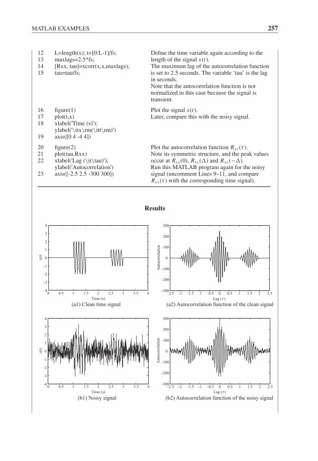
JWBK207-08 JWBK207-Shin January 18, 2008 10:6 Char Count= 0
MATLAB EXAMPLES 257
12131415
L=length(x); t=[0:L-1]/fs;maxlags=2.5*fs;[Rxx, tau]=xcorr(x,x,maxlags);tau=tau/fs;
Define the time variable again according to thelength of the signal x(t).The maximum lag of the autocorrelation functionis set to 2.5 seconds. The variable ‘tau’ is the lagin seconds.Note that the autocorrelation function is notnormalized in this case because the signal istransient.
161718
19
figure(1)plot(t,x)xlabel('Time (s)');ylabel('\itx\rm(\itt\rm)')axis([0 4 -4 4])
Plot the signal x(t).Later, compare this with the noisy signal.
202122
23
figure(2)plot(tau,Rxx)xlabel('Lag (\it\tau)');ylabel('Autocorrelation')axis([-2.5 2.5 -300 300])
Plot the autocorrelation function Rxx (τ ).Note its symmetric structure, and the peak valuesoccur at Rxx (0), Rxx (�) and Rxx (−�).Run this MATLAB program again for the noisysignal (uncomment Lines 9–11, and compareRxx (τ ) with the corresponding time signal).
Results
–2.5 –2 –1.5 –1 –0.5 0 0.5 1 1.5 2 2.5–300
–200
–100
0
100
200
300
Lag (τ )
Au
toco
rrel
atio
n
0 0.5 1 1.5 2 2.5 3 3.5 4–4
–3
–2
–1
0
1
2
3
4
Time (s)
(a1) Clean time signal
x(t)
(a2) Autocorrelation function of the clean signal
0 0.5 1 1.5 2 2.5 3 3.5 4–4
–3
–2
–1
0
1
2
3
4
Time (s)
(b1) Noisy signal
x(t)
–2.5 –2 –1.5 –1 –0.5 0 0.5 1 1.5 2 2.5–300
–200
–100
0
100
200
300
Lag (τ )
Au
toco
rrel
atio
n
(b2) Autocorrelation function of the noisy signal
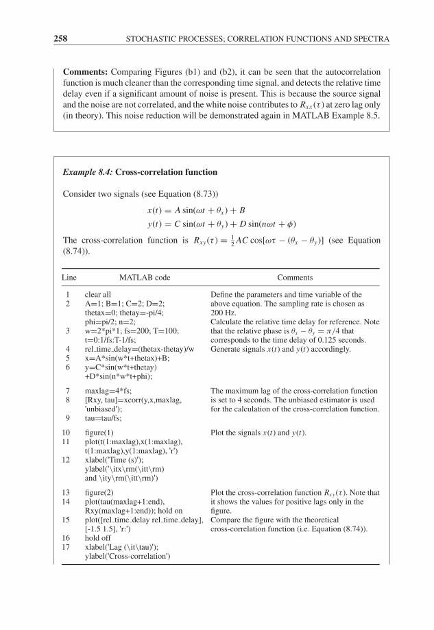
JWBK207-08 JWBK207-Shin January 18, 2008 10:6 Char Count= 0
258 STOCHASTIC PROCESSES; CORRELATION FUNCTIONS AND SPECTRA
Comments: Comparing Figures (b1) and (b2), it can be seen that the autocorrelationfunction is much cleaner than the corresponding time signal, and detects the relative timedelay even if a significant amount of noise is present. This is because the source signaland the noise are not correlated, and the white noise contributes to Rxx (τ ) at zero lag only(in theory). This noise reduction will be demonstrated again in MATLAB Example 8.5.
Example 8.4: Cross-correlation function
Consider two signals (see Equation (8.73))
x(t) = A sin(ωt + θx ) + B
y(t) = C sin(ωt + θy) + D sin(nωt + φ)
The cross-correlation function is Rxy(τ ) = 12
AC cos[ωτ − (θx − θy)] (see Equation(8.74)).
Line MATLAB code Comments
12
3
456
clear allA=1; B=1; C=2; D=2;thetax=0; thetay=-pi/4;phi=pi/2; n=2;w=2*pi*1; fs=200; T=100;t=0:1/fs:T-1/fs;rel time delay=(thetax-thetay)/wx=A*sin(w*t+thetax)+B;y=C*sin(w*t+thetay)+D*sin(n*w*t+phi);
Define the parameters and time variable of theabove equation. The sampling rate is chosen as200 Hz.Calculate the relative time delay for reference. Notethat the relative phase is θx − θy = π/4 thatcorresponds to the time delay of 0.125 seconds.Generate signals x(t) and y(t) accordingly.
78
9
maxlag=4*fs;[Rxy, tau]=xcorr(y,x,maxlag,'unbiased');tau=tau/fs;
The maximum lag of the cross-correlation functionis set to 4 seconds. The unbiased estimator is usedfor the calculation of the cross-correlation function.
1011
12
figure(1)plot(t(1:maxlag),x(1:maxlag),t(1:maxlag),y(1:maxlag), 'r')xlabel('Time (s)');ylabel('\itx\rm(\itt\rm)and \ity\rm(\itt\rm)')
Plot the signals x(t) and y(t).
1314
15
1617
figure(2)plot(tau(maxlag+1:end),Rxy(maxlag+1:end)); hold onplot([rel time delay rel time delay],[-1.5 1.5], 'r:')hold offxlabel('Lag (\it\tau)');ylabel('Cross-correlation')
Plot the cross-correlation function Rxy(τ ). Note thatit shows the values for positive lags only in thefigure.Compare the figure with the theoreticalcross-correlation function (i.e. Equation (8.74)).
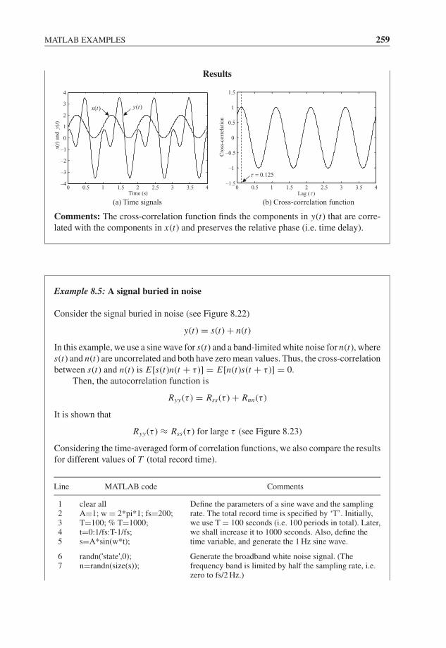
JWBK207-08 JWBK207-Shin January 18, 2008 10:6 Char Count= 0
MATLAB EXAMPLES 259
Results
0 0.5 1 1.5 2 2.5 3 3.5 4–4
–3
–2
–1
0
1
2
3
4
Time (s)
(a) Time signals
x(t)
and y
(t)
( )x t ( )y t
0 0.5 1 1.5 2 2.5 3 3.5 4–1.5
–1
–0.5
0
0.5
1
1.5
Lag (τ )
Cro
ss-c
orr
elat
ion
0.125τ =
(b) Cross-correlation function
Comments: The cross-correlation function finds the components in y(t) that are corre-lated with the components in x(t) and preserves the relative phase (i.e. time delay).
Example 8.5: A signal buried in noise
Consider the signal buried in noise (see Figure 8.22)
y(t) = s(t) + n(t)
In this example, we use a sine wave for s(t) and a band-limited white noise for n(t), wheres(t) and n(t) are uncorrelated and both have zero mean values. Thus, the cross-correlationbetween s(t) and n(t) is E[s(t)n(t + τ )] = E[n(t)s(t + τ )] = 0.
Then, the autocorrelation function is
Ryy(τ ) = Rss(τ ) + Rnn(τ )
It is shown that
Ryy(τ ) ≈ Rss(τ ) for large τ (see Figure 8.23)
Considering the time-averaged form of correlation functions, we also compare the resultsfor different values of T (total record time).
Line MATLAB code Comments
12345
clear allA=1; w = 2*pi*1; fs=200;T=100; % T=1000;t=0:1/fs:T-1/fs;s=A*sin(w*t);
Define the parameters of a sine wave and the samplingrate. The total record time is specified by ‘T’. Initially,we use T = 100 seconds (i.e. 100 periods in total). Later,we shall increase it to 1000 seconds. Also, define thetime variable, and generate the 1 Hz sine wave.
67
randn('state',0);n=randn(size(s));
Generate the broadband white noise signal. (Thefrequency band is limited by half the sampling rate, i.e.zero to fs/2 Hz.)
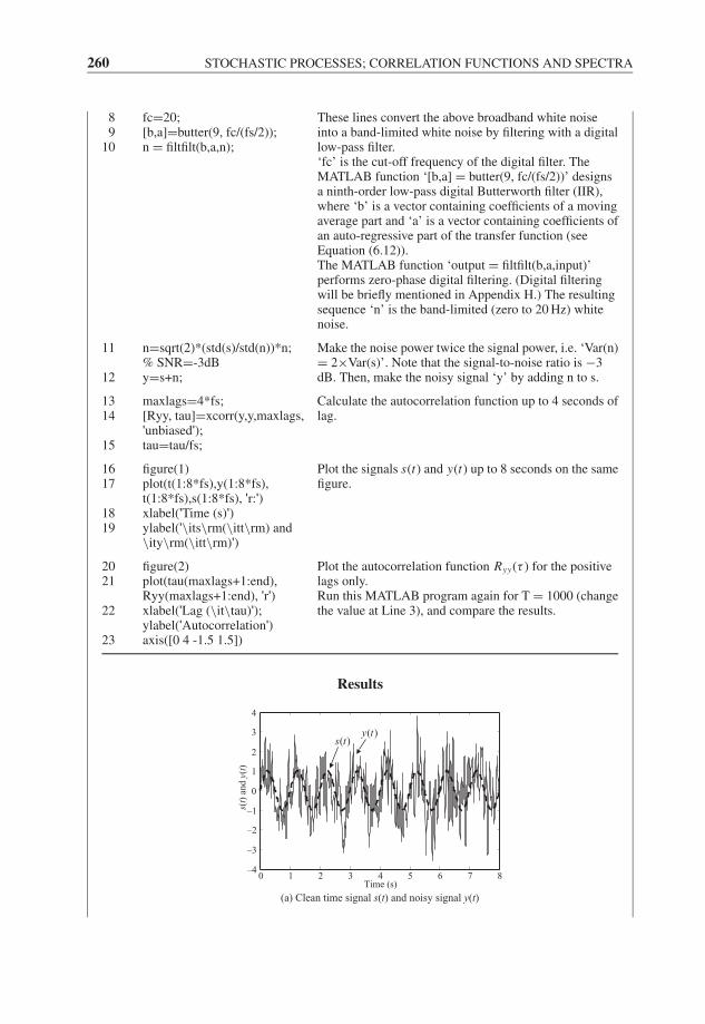
JWBK207-08 JWBK207-Shin January 18, 2008 10:6 Char Count= 0
260 STOCHASTIC PROCESSES; CORRELATION FUNCTIONS AND SPECTRA
89
10
fc=20;[b,a]=butter(9, fc/(fs/2));n = filtfilt(b,a,n);
These lines convert the above broadband white noiseinto a band-limited white noise by filtering with a digitallow-pass filter.‘fc’ is the cut-off frequency of the digital filter. TheMATLAB function ‘[b,a] = butter(9, fc/(fs/2))’ designsa ninth-order low-pass digital Butterworth filter (IIR),where ‘b’ is a vector containing coefficients of a movingaverage part and ‘a’ is a vector containing coefficients ofan auto-regressive part of the transfer function (seeEquation (6.12)).The MATLAB function ‘output = filtfilt(b,a,input)’performs zero-phase digital filtering. (Digital filteringwill be briefly mentioned in Appendix H.) The resultingsequence ‘n’ is the band-limited (zero to 20 Hz) whitenoise.
11
12
n=sqrt(2)*(std(s)/std(n))*n;% SNR=-3dBy=s+n;
Make the noise power twice the signal power, i.e. ‘Var(n)= 2×Var(s)’. Note that the signal-to-noise ratio is −3dB. Then, make the noisy signal ‘y’ by adding n to s.
1314
15
maxlags=4*fs;[Ryy, tau]=xcorr(y,y,maxlags,'unbiased');tau=tau/fs;
Calculate the autocorrelation function up to 4 seconds oflag.
1617
1819
figure(1)plot(t(1:8*fs),y(1:8*fs),t(1:8*fs),s(1:8*fs), 'r:')xlabel('Time (s)')ylabel('\its\rm(\itt\rm) and\ity\rm(\itt\rm)')
Plot the signals s(t) and y(t) up to 8 seconds on the samefigure.
2021
22
23
figure(2)plot(tau(maxlags+1:end),Ryy(maxlags+1:end), 'r')xlabel('Lag (\it\tau)');ylabel('Autocorrelation')axis([0 4 -1.5 1.5])
Plot the autocorrelation function Ryy(τ ) for the positivelags only.Run this MATLAB program again for T = 1000 (changethe value at Line 3), and compare the results.
Results
0 1 2 3 4 5 6 7 8–4
–3
–2
–1
0
1
2
3
4
Time (s)
s(t)
and y
(t)
( )y t( )s t
(a) Clean time signal s(t) and noisy signal y(t)
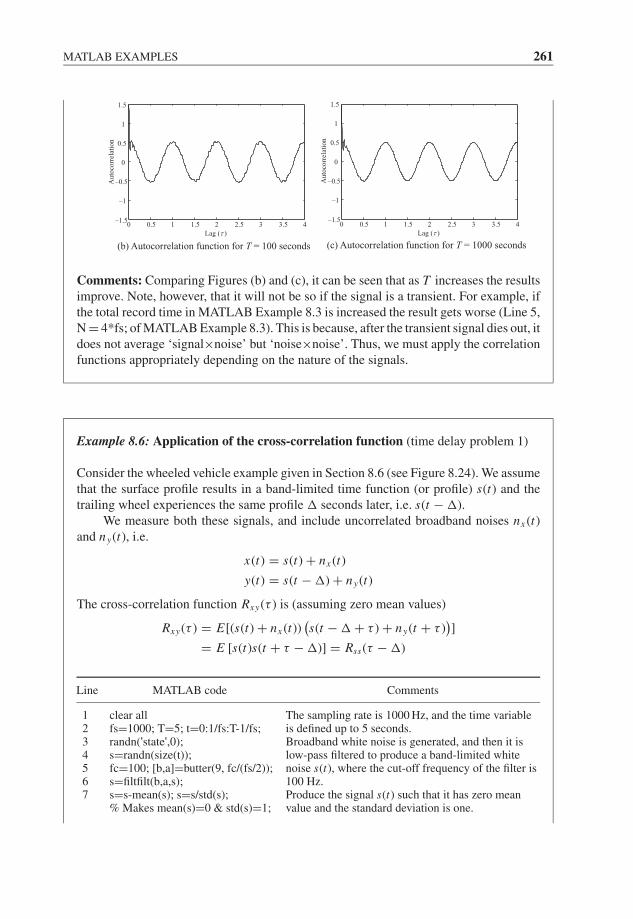
JWBK207-08 JWBK207-Shin January 18, 2008 10:6 Char Count= 0
MATLAB EXAMPLES 261
0 0.5 1 1.5
(b) Autocorrelation function for T = 100 seconds
2 2.5 3 3.5 4–1.5
–1
–0.5
0
0.5
1
1.5
Lag (τ )
Auto
corr
elat
ion
0 0.5 1 1.5 2 2.5 3 3.5 4–1.5
–1
–0.5
0
0.5
1
1.5
Lag (τ )
Auto
corr
elat
ion
(c) Autocorrelation function for T = 1000 seconds
Comments: Comparing Figures (b) and (c), it can be seen that as T increases the resultsimprove. Note, however, that it will not be so if the signal is a transient. For example, ifthe total record time in MATLAB Example 8.3 is increased the result gets worse (Line 5,N = 4*fs; of MATLAB Example 8.3). This is because, after the transient signal dies out, itdoes not average ‘signal×noise’ but ‘noise×noise’. Thus, we must apply the correlationfunctions appropriately depending on the nature of the signals.
Example 8.6: Application of the cross-correlation function (time delay problem 1)
Consider the wheeled vehicle example given in Section 8.6 (see Figure 8.24). We assumethat the surface profile results in a band-limited time function (or profile) s(t) and thetrailing wheel experiences the same profile � seconds later, i.e. s(t − �).
We measure both these signals, and include uncorrelated broadband noises nx (t)and ny(t), i.e.
x(t) = s(t) + nx (t)
y(t) = s(t − �) + ny(t)
The cross-correlation function Rxy(τ ) is (assuming zero mean values)
Rxy(τ ) = E[(s(t) + nx (t))(s(t − � + τ ) + ny(t + τ )
)]
= E [s(t)s(t + τ − �)] = Rss(τ − �)
Line MATLAB code Comments
1234567
clear allfs=1000; T=5; t=0:1/fs:T-1/fs;randn('state',0);s=randn(size(t));fc=100; [b,a]=butter(9, fc/(fs/2));s=filtfilt(b,a,s);s=s-mean(s); s=s/std(s);% Makes mean(s)=0 & std(s)=1;
The sampling rate is 1000 Hz, and the time variableis defined up to 5 seconds.Broadband white noise is generated, and then it islow-pass filtered to produce a band-limited whitenoise s(t), where the cut-off frequency of the filter is100 Hz.Produce the signal s(t) such that it has zero meanvalue and the standard deviation is one.
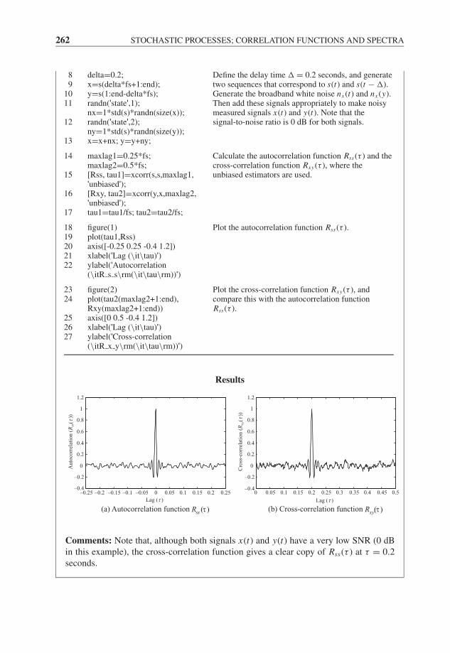
JWBK207-08 JWBK207-Shin January 18, 2008 10:6 Char Count= 0
262 STOCHASTIC PROCESSES; CORRELATION FUNCTIONS AND SPECTRA
89
1011
12
13
delta=0.2;x=s(delta*fs+1:end);y=s(1:end-delta*fs);randn('state',1);nx=1*std(s)*randn(size(x));randn('state',2);ny=1*std(s)*randn(size(y));x=x+nx; y=y+ny;
Define the delay time � = 0.2 seconds, and generatetwo sequences that correspond to s(t) and s(t − �).Generate the broadband white noise nx (t) and nx (y).Then add these signals appropriately to make noisymeasured signals x(t) and y(t). Note that thesignal-to-noise ratio is 0 dB for both signals.
14
15
16
17
maxlag1=0.25*fs;maxlag2=0.5*fs;[Rss, tau1]=xcorr(s,s,maxlag1,'unbiased');[Rxy, tau2]=xcorr(y,x,maxlag2,'unbiased');tau1=tau1/fs; tau2=tau2/fs;
Calculate the autocorrelation function Rss(τ ) and thecross-correlation function Rxy(τ ), where theunbiased estimators are used.
1819202122
figure(1)plot(tau1,Rss)axis([-0.25 0.25 -0.4 1.2])xlabel('Lag (\it\tau)')ylabel('Autocorrelation(\itR s s\rm(\it\tau\rm))')
Plot the autocorrelation function Rss(τ ).
2324
252627
figure(2)plot(tau2(maxlag2+1:end),Rxy(maxlag2+1:end))axis([0 0.5 -0.4 1.2])xlabel('Lag (\it\tau)')ylabel('Cross-correlation(\itR x y\rm(\it\tau\rm))')
Plot the cross-correlation function Rxy(τ ), andcompare this with the autocorrelation functionRss(τ ).
Results
–0.25 –0.2 –0.15 –0.1 –0.05 0 0.05 0.1 0.15 0.2 0.25–0.4
–0.2
0
0.2
0.4
0.6
0.8
1
1.2
Lag (τ )
Au
toco
rrel
atio
n (
Rss
( τ))
0 0.05 0.1 0.15 0.2 0.25 0.3 0.35 0.4 0.45 0.5–0.4
–0.2
0
0.2
0.4
0.6
0.8
1
1.2
Lag (τ )
Cro
ss-c
orr
elat
ion
(R
xy(τ
))
(a) Autocorrelation function ( )ssR τ (b) Cross-correlation function ( )xyR τ
Comments: Note that, although both signals x(t) and y(t) have a very low SNR (0 dBin this example), the cross-correlation function gives a clear copy of Rss(τ ) at τ = 0.2seconds.
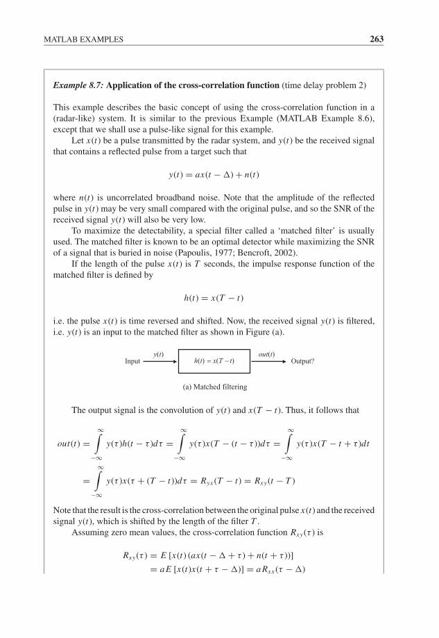
JWBK207-08 JWBK207-Shin January 18, 2008 10:6 Char Count= 0
MATLAB EXAMPLES 263
Example 8.7: Application of the cross-correlation function (time delay problem 2)
This example describes the basic concept of using the cross-correlation function in a(radar-like) system. It is similar to the previous Example (MATLAB Example 8.6),except that we shall use a pulse-like signal for this example.
Let x(t) be a pulse transmitted by the radar system, and y(t) be the received signalthat contains a reflected pulse from a target such that
y(t) = ax(t − �) + n(t)
where n(t) is uncorrelated broadband noise. Note that the amplitude of the reflectedpulse in y(t) may be very small compared with the original pulse, and so the SNR of thereceived signal y(t) will also be very low.
To maximize the detectability, a special filter called a ‘matched filter’ is usuallyused. The matched filter is known to be an optimal detector while maximizing the SNRof a signal that is buried in noise (Papoulis, 1977; Bencroft, 2002).
If the length of the pulse x(t) is T seconds, the impulse response function of thematched filter is defined by
h(t) = x(T − t)
i.e. the pulse x(t) is time reversed and shifted. Now, the received signal y(t) is filtered,i.e. y(t) is an input to the matched filter as shown in Figure (a).
(a) Matched filtering
y(t)h(t) x(T t)= − Output?
out(t)Input
The output signal is the convolution of y(t) and x(T − t). Thus, it follows that
out(t) =∞∫
−∞y(τ )h(t − τ )dτ =
∞∫−∞
y(τ )x(T − (t − τ ))dτ =∞∫
−∞y(τ )x(T − t + τ )dt
=∞∫
−∞y(τ )x(τ + (T − t))dτ = Ryx (T − t) = Rxy(t − T )
Note that the result is the cross-correlation between the original pulse x(t) and the receivedsignal y(t), which is shifted by the length of the filter T .
Assuming zero mean values, the cross-correlation function Rxy(τ ) is
Rxy(τ ) = E [x(t) (ax(t − � + τ ) + n(t + τ ))]
= aE [x(t)x(t + τ − �)] = a Rxx (τ − �)
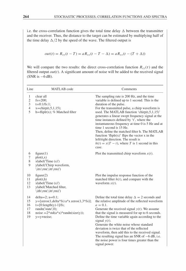
JWBK207-08 JWBK207-Shin January 18, 2008 10:6 Char Count= 0
264 STOCHASTIC PROCESSES; CORRELATION FUNCTIONS AND SPECTRA
i.e. the cross-correlation function gives the total time delay � between the transmitterand the receiver. Thus, the distance to the target can be estimated by multiplying half ofthe time delay �/2 by the speed of the wave. The filtered output is
out(t) = Rxy(t − T ) = a Rxx (t − T − �) = a Rxx (t − (T + �))
We will compare the two results: the direct cross-correlation function Rxy(τ ) and thefiltered output out(t). A significant amount of noise will be added to the received signal(SNR is −6 dB).
Line MATLAB code Comments
12345
clear allfs=200;t=0:1/fs:1;x=chirp(t,5,1,15);h=fliplr(x); % Matched filter
The sampling rate is 200 Hz, and the timevariable is defined up to 1 second. This is theduration of the pulse.For the transmitted pulse, a chirp waveform isused. The MATLAB function ‘chirp(t,5,1,15)’generates a linear swept frequency signal at thetime instances defined by ‘t’, where theinstantaneous frequency at time 0 is 5 Hz and attime 1 second is 15 Hz.Then, define the matched filter h. The MATLABfunction ‘fliplr(x)’ flips the vector x in theleft/right direction. The result ish(t) = x(T − t), where T is 1 second in thiscase.
6789
figure(1)plot(t,x)xlabel('Time (s)')ylabel('Chirp waveform,\itx\rm(\itt\rm)')
Plot the transmitted chirp waveform x(t).
10111213
figure(2)plot(t,h)xlabel('Time (s)')ylabel('Matched filter,\ith\rm(\itt\rm)')
Plot the impulse response function of thematched filter h(t), and compare with thewaveform x(t).
141516171819
delta=2; a=0.1;y=[zeros(1,delta*fs) a*x zeros(1,3*fs)];t=[0:length(y)-1]/fs;randn('state',0);noise =2*std(a*x)*randn(size(y));y=y+noise;
Define the total time delay � = 2 seconds andthe relative amplitude of the reflected waveforma = 0.1.Generate the received signal y(t). We assumethat the signal is measured for up to 6 seconds.Define the time variable again according to thesignal y(t).Generate the white noise whose standarddeviation is twice that of the reflectedwaveform, then add this to the received signal.The resulting signal has an SNR of −6 dB, i.e.the noise power is four times greater than thesignal power.
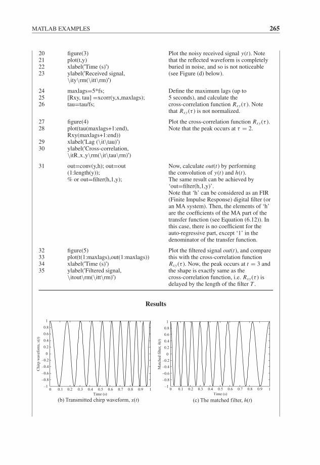
JWBK207-08 JWBK207-Shin January 18, 2008 10:6 Char Count= 0
MATLAB EXAMPLES 265
20212223
figure(3)plot(t,y)xlabel('Time (s)')ylabel('Received signal,\ity\rm(\itt\rm)')
Plot the noisy received signal y(t). Notethat the reflected waveform is completelyburied in noise, and so is not noticeable(see Figure (d) below).
242526
maxlags=5*fs;[Rxy, tau] =xcorr(y,x,maxlags);tau=tau/fs;
Define the maximum lags (up to5 seconds), and calculate thecross-correlation function Rxy(τ ). Notethat Rxy(τ ) is not normalized.
2728
2930
figure(4)plot(tau(maxlags+1:end),Rxy(maxlags+1:end))xlabel('Lag (\it\tau)')ylabel('Cross-correlation,\itR x y\rm(\it\tau\rm)')
Plot the cross-correlation function Rxy(τ ).Note that the peak occurs at τ = 2.
31 out=conv(y,h); out=out(1:length(y));% or out=filter(h,1,y);
Now, calculate out(t) by performingthe convolution of y(t) and h(t).The same result can be achieved by‘out=filter(h,1,y)’.Note that ‘h’ can be considered as an FIR(Finite Impulse Response) digital filter (oran MA system). Then, the elements of ‘h’are the coefficients of the MA part of thetransfer function (see Equation (6.12)). Inthis case, there is no coefficient for theauto-regressive part, except ‘1’ in thedenominator of the transfer function.
32333435
figure(5)plot(t(1:maxlags),out(1:maxlags))xlabel('Time (s)')ylabel('Filtered signal,\itout\rm(\itt\rm)')
Plot the filtered signal out(t), and comparethis with the cross-correlation functionRxy(τ ). Now, the peak occurs at t = 3 andthe shape is exactly same as thecross-correlation function, i.e. Rxy(τ ) isdelayed by the length of the filter T .
Results
0 0.1 0.2
(c) The matched filter, h(t)
0.3 0 0.1 0.2 0.3 0.4 0.5 0.6 0.7 0.8 0.9 1–1
–0.8
–0.6
–0.4
–0.2
0
0.2
0.4
0.6
0.8
1
Time (s)
Mat
ched
fil
ter,
h(t
)
0.4 0.5 0.6 0.7 0.8 0.9 1–1
–0.8
–0.6
–0.4
–0.2
0
0.2
0.4
0.6
0.8
1
Time (s)
Chir
p w
avef
orm
, x(
t)
(b) Transmitted chirp waveform, x(t)
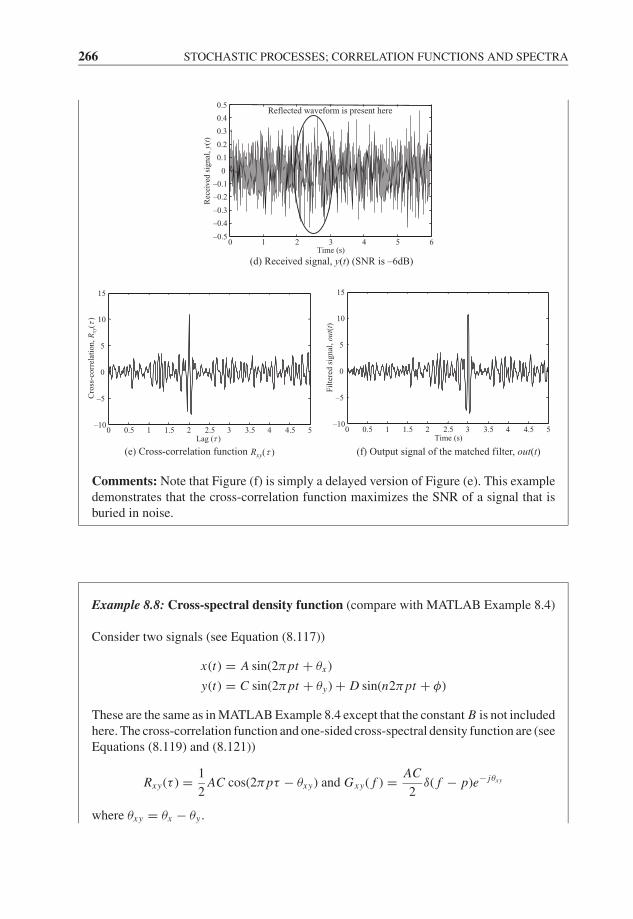
JWBK207-08 JWBK207-Shin January 18, 2008 10:6 Char Count= 0
266 STOCHASTIC PROCESSES; CORRELATION FUNCTIONS AND SPECTRA
0 1 2 3 4 5 6–0.5
–0.4
–0.3
–0.2
–0.1
0
0.1
0.2
0.3
0.4
0.5
Time (s)
Rec
eived
sig
nal
, y(
t)
Reflected
(d) Received signal, y(t) (SNR is –6dB)
waveform is present here
0 0.5 1 1.5 2 2.5 3 3.5 4 4.5 5–10
–5
0
5
10
15
Lag (τ )
Cro
ss-c
orr
elat
ion,
Rxy
( τ)
(e) Cross-correlation function Rxy(τ )
0 0.5 1 1.5 2 2.5 3 3.5 4 4.5 5–10
–5
0
5
10
15
Time (s)
Fil
tere
d s
ignal
, ou
t(t)
(f) Output signal of the matched filter, out(t)
Comments: Note that Figure (f) is simply a delayed version of Figure (e). This exampledemonstrates that the cross-correlation function maximizes the SNR of a signal that isburied in noise.
Example 8.8: Cross-spectral density function (compare with MATLAB Example 8.4)
Consider two signals (see Equation (8.117))
x(t) = A sin(2πpt + θx )
y(t) = C sin(2πpt + θy) + D sin(n2πpt + φ)
These are the same as in MATLAB Example 8.4 except that the constant B is not includedhere. The cross-correlation function and one-sided cross-spectral density function are (seeEquations (8.119) and (8.121))
Rxy(τ ) = 1
2AC cos(2πpτ − θxy) and Gxy( f ) = AC
2δ( f − p)e− jθxy
where θxy = θx − θy .
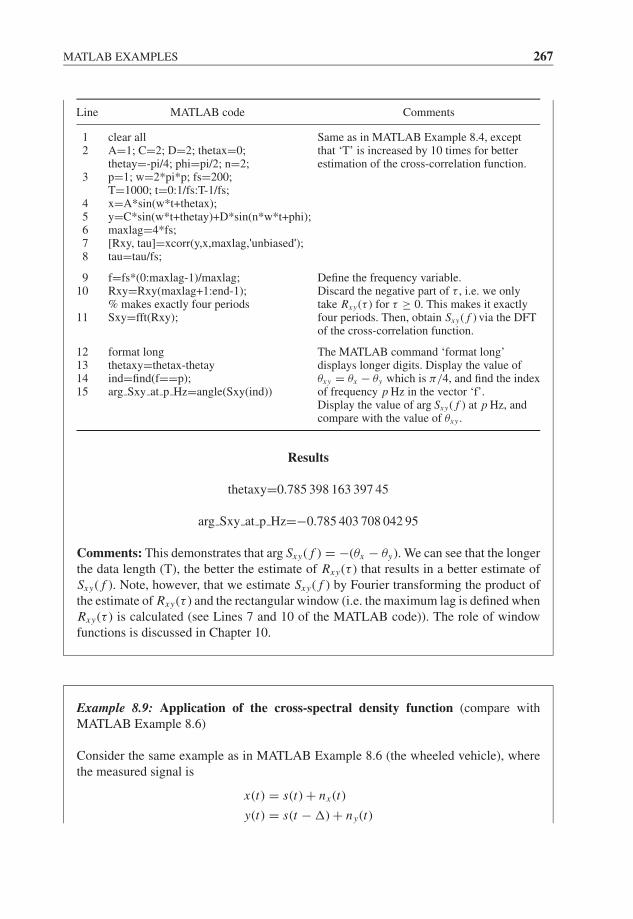
JWBK207-08 JWBK207-Shin January 18, 2008 10:6 Char Count= 0
MATLAB EXAMPLES 267
Line MATLAB code Comments
12
3
45678
clear allA=1; C=2; D=2; thetax=0;thetay=-pi/4; phi=pi/2; n=2;p=1; w=2*pi*p; fs=200;T=1000; t=0:1/fs:T-1/fs;x=A*sin(w*t+thetax);y=C*sin(w*t+thetay)+D*sin(n*w*t+phi);maxlag=4*fs;[Rxy, tau]=xcorr(y,x,maxlag,'unbiased');tau=tau/fs;
Same as in MATLAB Example 8.4, exceptthat ‘T’ is increased by 10 times for betterestimation of the cross-correlation function.
910
11
f=fs*(0:maxlag-1)/maxlag;Rxy=Rxy(maxlag+1:end-1);% makes exactly four periodsSxy=fft(Rxy);
Define the frequency variable.Discard the negative part of τ , i.e. we onlytake Rxy(τ ) for τ ≥ 0. This makes it exactlyfour periods. Then, obtain Sxy( f ) via the DFTof the cross-correlation function.
12131415
format longthetaxy=thetax-thetayind=find(f==p);arg Sxy at p Hz=angle(Sxy(ind))
The MATLAB command ‘format long’displays longer digits. Display the value ofθxy = θx − θy which is π/4, and find the indexof frequency p Hz in the vector ‘f’.Display the value of arg Sxy( f ) at p Hz, andcompare with the value of θxy .
Results
thetaxy=0.785 398 163 397 45
arg Sxy at p Hz=−0.785 403 708 042 95
Comments: This demonstrates that arg Sxy( f ) = −(θx − θy). We can see that the longerthe data length (T), the better the estimate of Rxy(τ ) that results in a better estimate ofSxy( f ). Note, however, that we estimate Sxy( f ) by Fourier transforming the product ofthe estimate of Rxy(τ ) and the rectangular window (i.e. the maximum lag is defined whenRxy(τ ) is calculated (see Lines 7 and 10 of the MATLAB code)). The role of windowfunctions is discussed in Chapter 10.
Example 8.9: Application of the cross-spectral density function (compare withMATLAB Example 8.6)
Consider the same example as in MATLAB Example 8.6 (the wheeled vehicle), wherethe measured signal is
x(t) = s(t) + nx (t)
y(t) = s(t − �) + ny(t)

JWBK207-08 JWBK207-Shin January 18, 2008 10:6 Char Count= 0
268 STOCHASTIC PROCESSES; CORRELATION FUNCTIONS AND SPECTRA
and the cross-correlation function and the cross-spectral density function are
Rxy(τ ) = Rss(τ − �) and Sxy( f ) = H ( f )Sss( f ) = e− j2π f �Sss( f )
First, we shall estimate � using Sxy( f ). Then, by forming the ratio Sxy( f )/Sxx ( f ) weshall estimate the frequency response function H ( f ) from which the time delay � canalso be estimated. Note that we are not using Sxy( f )/Sss( f ), but the following:
H1( f ) = Sxy( f )
Sxx ( f )= Sxy( f )
Sss( f ) + Snx nx ( f )(1)
Since Rnx nx (τ ) is an even function, Snx nx ( f ) is real valued, i.e. arg Snx nx ( f ) = 0. Thus, itcan be shown that
arg H ( f ) = arg H1( f ) = −2π f �
Note that H1( f ) may underestimate the magnitude of H ( f ) depending on the variance ofthe noise. However, the phase of H1( f ) is not affected by uncorrelated noise, i.e. we cansee that the phase of H1( f ) is less sensitive to noise than the magnitude of H1( f ). Moredetails of the estimator H1( f ) defined by Equation (1) will be discussed in Chapter 9.
Line MATLAB code Comments
1234567
89
1011
12
1314151617
clear allfs=500; T=100; t=0:1/fs:T-1/fs;randn('state',0);s=randn(size(t));fc=100; [b,a]=butter(9,fc/(fs/2));s=filtfilt(b,a,s);s=s-mean(s); s=s/std(s);% Makes mean(s)=0 & std(s)=1;delta=0.2;x=s(delta*fs+1:end);y=s(1:end-delta*fs);randn('state',1);nx=1*std(s)*randn(size(x));randn('state',2);ny=1*std(s)*randn(size(y));x=x+nx; y=y+ny;maxlag=fs;[Rxx, tau]=xcorr(x,x,maxlag, 'unbiased');[Rxy, tau]=xcorr(y,x,maxlag, 'unbiased');tau=tau/fs;
Same as in MATLAB Example 8.6,except that the sampling rate is reducedand the total record time ‘T’ is increased.Note that the delay time � = 0.2 secondsas before.Note also that the same number of lags isused for both autocorrelation andcross-correlation functions.
181920
f=fs*(0:maxlag-1)/maxlag;Rxy 1=Rxy(maxlag+1:end-1);Sxy=fft(Rxy 1);
Define the frequency variable.Discard the negative part of τ , i.e. weonly take Rxy(τ ) for τ ≥ 0. If we includethe negative part of τ when the DFT isperformed, then the result is a puredelay. If this is the case, we mustcompensate for this delay.
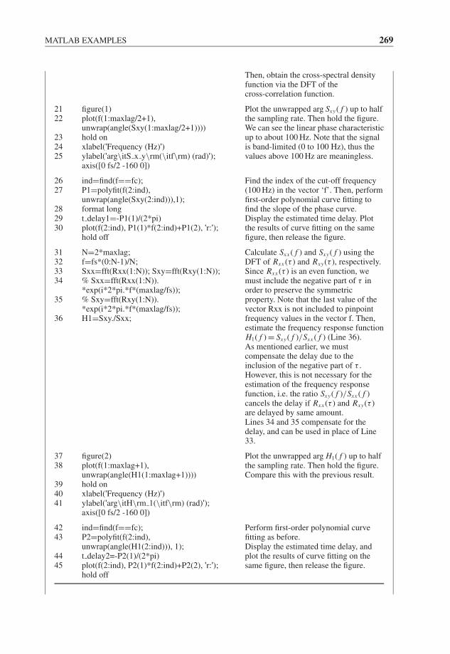
JWBK207-08 JWBK207-Shin January 18, 2008 10:6 Char Count= 0
MATLAB EXAMPLES 269
Then, obtain the cross-spectral densityfunction via the DFT of thecross-correlation function.
2122
232425
figure(1)plot(f(1:maxlag/2+1),unwrap(angle(Sxy(1:maxlag/2+1))))hold onxlabel('Frequency (Hz)')ylabel('arg\itS x y\rm(\itf\rm) (rad)');axis([0 fs/2 -160 0])
Plot the unwrapped arg Sxy( f ) up to halfthe sampling rate. Then hold the figure.We can see the linear phase characteristicup to about 100 Hz. Note that the signalis band-limited (0 to 100 Hz), thus thevalues above 100 Hz are meaningless.
2627
282930
ind=find(f==fc);P1=polyfit(f(2:ind),unwrap(angle(Sxy(2:ind))),1);format longt delay1=-P1(1)/(2*pi)plot(f(2:ind), P1(1)*f(2:ind)+P1(2), 'r:');hold off
Find the index of the cut-off frequency(100 Hz) in the vector ‘f’. Then, performfirst-order polynomial curve fitting tofind the slope of the phase curve.Display the estimated time delay. Plotthe results of curve fitting on the samefigure, then release the figure.
31323334
35
36
N=2*maxlag;f=fs*(0:N-1)/N;Sxx=fft(Rxx(1:N)); Sxy=fft(Rxy(1:N));% Sxx=fft(Rxx(1:N)).*exp(i*2*pi.*f*(maxlag/fs));% Sxy=fft(Rxy(1:N)).*exp(i*2*pi.*f*(maxlag/fs));H1=Sxy./Sxx;
Calculate Sxx ( f ) and Sxy( f ) using theDFT of Rxx (τ ) and Rxy(τ ), respectively.Since Rxx (τ ) is an even function, wemust include the negative part of τ inorder to preserve the symmetricproperty. Note that the last value of thevector Rxx is not included to pinpointfrequency values in the vector f. Then,estimate the frequency response functionH1( f ) = Sxy( f )/Sxx ( f ) (Line 36).As mentioned earlier, we mustcompensate the delay due to theinclusion of the negative part of τ .However, this is not necessary for theestimation of the frequency responsefunction, i.e. the ratio Sxy( f )/Sxx ( f )cancels the delay if Rxx (τ ) and Rxy(τ )are delayed by same amount.Lines 34 and 35 compensate for thedelay, and can be used in place of Line33.
3738
394041
figure(2)plot(f(1:maxlag+1),unwrap(angle(H1(1:maxlag+1))))hold onxlabel('Frequency (Hz)')ylabel('arg\itH\rm 1(\itf\rm) (rad)');axis([0 fs/2 -160 0])
Plot the unwrapped arg H1( f ) up to halfthe sampling rate. Then hold the figure.Compare this with the previous result.
4243
4445
ind=find(f==fc);P2=polyfit(f(2:ind),unwrap(angle(H1(2:ind))), 1);t delay2=-P2(1)/(2*pi)plot(f(2:ind), P2(1)*f(2:ind)+P2(2), 'r:');hold off
Perform first-order polynomial curvefitting as before.Display the estimated time delay, andplot the results of curve fitting on thesame figure, then release the figure.
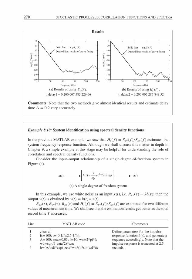
JWBK207-08 JWBK207-Shin January 18, 2008 10:6 Char Count= 0
270 STOCHASTIC PROCESSES; CORRELATION FUNCTIONS AND SPECTRA
Results
1Solid line: arg ( )
Dashed line: results of curve fitting
H f
0 50 100 150 200 250–160
–140
–120
–100
–80
–60
–40
–20
0
Frequency (Hz)
arg
H1(f
) (r
ad)
0 50 100 150 200 250–160
–140
–120
–100
–80
–60
–40
–20
0
arg
S xy(
f)
t_delay1 = 0.200 007 583 226 06
(a) Results of using ,Sxy(f )
(rad
)
Solid line: arg ( )
Dashed line: results of curve fitting
xyS f
Frequency (Hz)
(b) Results of using ,H1 (f )
t_delay2 = 0.200 005 287 848 52
Comments: Note that the two methods give almost identical results and estimate delaytime � = 0.2 very accurately.
Example 8.10: System identification using spectral density functions
In the previous MATLAB example, we saw that H1( f ) = Sxy( f )/Sxx ( f ) estimates thesystem frequency response function. Although we shall discuss this matter in depth inChapter 9, a simple example at this stage may be helpful for understanding the role ofcorrelation and spectral density functions.
Consider the input–output relationship of a single-degree-of-freedom system inFigure (a).
(a) A single-degree-of-freedom system
( )x t ( ) sinntd
d
Ah t e tζω ω
ω−= ( )y t
In this example, we use white noise as an input x(t), i.e. Rxx (τ ) = kδ(τ ); then theoutput y(t) is obtained by y(t) = h(t) ∗ x(t).
Rxx (τ ), Ryy(τ ), Rxy(τ ) and H1( f ) = Sxy( f )/Sxx ( f ) are examined for two differentvalues of measurement time. We shall see that the estimation results get better as the totalrecord time T increases.
Line MATLAB code Comments
123
4
clear allfs=100; t=[0:1/fs:2.5-1/fs];A=100; zeta=0.03; f=10; wn=2*pi*f;wd=sqrt(1-zetaˆ2)*wn;h=(A/wd)*exp(-zeta*wn*t).*sin(wd*t);
Define parameters for the impulseresponse function h(t), and generate asequence accordingly. Note that theimpulse response is truncated at 2.5seconds.
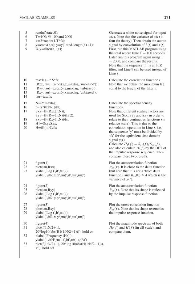
JWBK207-08 JWBK207-Shin January 18, 2008 10:6 Char Count= 0
MATLAB EXAMPLES 271
56789
randn('state',0);T=100; % 100 and 2000x=2*randn(1,T*fs);y=conv(h,x); y=y(1:end-length(h)+1);% y=filter(h,1,x);
Generate a white noise signal for inputx(t). Note that the variance of x(t) isfour (in theory). Then obtain the outputsignal by convolution of h(t) and x(t).First, run this MATLAB program usingthe total record time T = 100 seconds.Later run this program again using T= 2000, and compare the results.Note that the sequence ‘h’ is an FIRfilter, and Line 9 can be used instead ofLine 8.
1011121314
maxlag=2.5*fs;[Rxx, tau]=xcorr(x,x,maxlag, 'unbiased');[Ryy, tau]=xcorr(y,y,maxlag, 'unbiased');[Rxy, tau]=xcorr(y,x,maxlag, 'unbiased');tau=tau/fs;
Calculate the correlation functions.Note that we define the maximum lagequal to the length of the filter h.
151617
181920
N=2*maxlag;f=fs*(0:N-1)/N;Sxx=fft(Rxx(1:N));Syy=fft(Ryy(1:N))/(fsˆ2);Sxy=fft(Rxy(1:N))/fs;H1=Sxy./Sxx;H=fft(h,N)/fs;
Calculate the spectral densityfunctions.Note that different scaling factors areused for Sxx, Syy and Sxy in order torelate to their continuous functions (inrelative scale). This is due to theconvolution operation in Line 8, i.e.the sequence ‘y’ must be divided by‘fs’ for the equivalent time domainsignal y(t).Calculate H1( f ) = Sxy( f )/Sxx ( f ),and also calculate H ( f ) by the DFT ofthe impulse response sequence. Thencompare these two results.
212223
figure(1)plot(tau,Rxx)xlabel('Lag (\it\tau)');ylabel('\itR x x\rm(\it\tau\rm)')
Plot the autocorrelation functionRxx (τ ). It is close to the delta function(but note that it is not a ‘true’ deltafunction), and Rxx (0) ≈ 4 which is thevariance of x(t).
242526
figure(2)plot(tau,Ryy)xlabel('Lag (\it\tau)');ylabel('\itR y y\rm(\it\tau\rm)')
Plot the autocorrelation functionRyy(τ ). Note that its shape is reflectedby the impulse response function.
272829
figure(3)plot(tau,Rxy)xlabel('Lag (\it\tau)');ylabel('\itR x y\rm(\it\tau\rm)')
Plot the cross-correlation functionRxy(τ ). Note that its shape resemblesthe impulse response function.
3031
32
33
figure(4)plot(f(1:N/2+1),20*log10(abs(H1(1:N/2+1)))); hold onxlabel('Frequency (Hz)');ylabel('|\itH\rm 1(\itf\rm)| (dB)')plot(f(1:N/2+1), 20*log10(abs(H(1:N/2+1))),'r:'); hold off
Plot the magnitude spectrum of bothH1( f ) and H ( f ) (in dB scale), andcompare them.

JWBK207-08 JWBK207-Shin January 18, 2008 10:6 Char Count= 0
272 STOCHASTIC PROCESSES; CORRELATION FUNCTIONS AND SPECTRA
3435
36
37
figure(5)plot(f(1:N/2+1),unwrap(angle(H1(1:N/2+1)))); hold onxlabel('Frequency (Hz)');ylabel('arg\itH\rm 1(\itf\rm) (rad)')plot(f(1:N/2+1), unwrap(angle(H(1:N/2+1))),'r:'); hold off
Plot the phase spectrum of both H1( f )and H ( f ), and compare them. Runthis MATLAB program again for T =2000, and compare the results.
Results
T = 100 T = 2000
–2.5 –2 –1.5 –1 –0.5 0 0.5 1 1.5 2 2.5–0.5
0
0.5
1
1.5
2
2.5
3
3.5
4
4.5
Lag (τ )
Rxx
(τ)
–2.5 –2 –1.5 –1 –0.5 0 0.5 1 1.5 2 2.5–0.5
0
0.5
1
1.5
2
2.5
3
3.5
4
4.5
Lag (τ )
Rxx
(τ)
Rxx(τ )(b1) Autocorrelation function, Rxx(τ )(c1) Autocorrelation function,
–2.5 –2 –1.5 –1 –0.5 0 0.5 1 1.5 2 2.5–150
–100
–50
0
50
100
150
Lag (τ )
Ryy
( τ)
–2.5 –2 –1.5 –1 –0.5 0 0.5 1 1.5 2 2.5–150
–100
–50
0
50
100
150
Lag (τ )
Ryy
(τ)
Ryy(τ )(b2) Autocorrelation function, Ryy(τ )(c2) Autocorrelation function,
–2.5 –2 –1.5 –1 –0.5 0 0.5 1 1.5 2 2.5–6
–4
–2
0
2
4
6
Lag (τ )
Rxy
(τ)
Rxy
(τ)
–2.5 –2 –1.5 –1 –0.5 0 0.5 1 1.5 2 2.5–6
–4
–2
0
2
4
6
Lag (τ )
Rxy(τ )(b3) Cross-correlation function, Rxy(τ )(c3) Cross-correlation function,
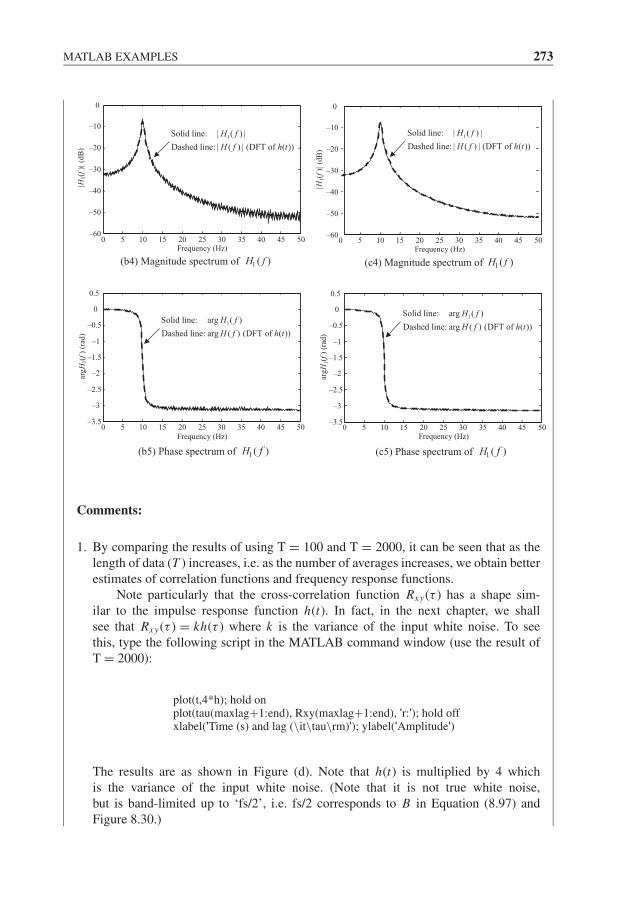
JWBK207-08 JWBK207-Shin January 18, 2008 10:6 Char Count= 0
MATLAB EXAMPLES 273
0 5 10 15 20 25 30 35 40 45 50–60
–50
–40
–30
–20
–10
0
Frequency (Hz)
|H1(f
)|(d
B)
1Solid line: | ( ) |
Dashed line: | ( ) | (DFT of ( ))
H f
f f
H f h t1Solid line: | ( ) |
Dashed line: | ( ) | (DFT of ( ))
H f
H f h t
|H1(f
)|(d
B)
0 5 10 15 20 25 30 35 40 45 50–60
–50
–40
–30
–20
–10
0
Frequency (Hz)
H1 ( )(b4) Magnitude spectrum of H1 ( )(c4) Magnitude spectrum of
0 5 10 15 20 25 30 35 40 45 50–3.5
–3
–2.5
–2
–1.5
–1
–0.5
0
0.5
Frequency (Hz)
arg
H1(f
) (r
ad)
1Solid line: arg ( )
Dashed line: arg ( ) (DFT of ( ))
H f
f
H f h t
1Solid line: arg ( )
Dashed line: arg ( ) (DFT of ( ))
H f
H f h tar
gH
1(f
) (r
ad)
0 5 10 15 20 25 30 35 40 45 50–3.5
–3
–2.5
–2
–1.5
–1
–0.5
0
0.5
Frequency (Hz)
H1 ( ) fH1 ( )(b5) Phase spectrum of (c5) Phase spectrum of
Comments:
1. By comparing the results of using T = 100 and T = 2000, it can be seen that as thelength of data (T ) increases, i.e. as the number of averages increases, we obtain betterestimates of correlation functions and frequency response functions.
Note particularly that the cross-correlation function Rxy(τ ) has a shape sim-ilar to the impulse response function h(t). In fact, in the next chapter, we shallsee that Rxy(τ ) = kh(τ ) where k is the variance of the input white noise. To seethis, type the following script in the MATLAB command window (use the result ofT = 2000):
plot(t,4*h); hold onplot(tau(maxlag+1:end), Rxy(maxlag+1:end), 'r:'); hold offxlabel('Time (s) and lag (\it\tau\rm)'); ylabel('Amplitude')
The results are as shown in Figure (d). Note that h(t) is multiplied by 4 whichis the variance of the input white noise. (Note that it is not true white noise,but is band-limited up to ‘fs/2’, i.e. fs/2 corresponds to B in Equation (8.97) andFigure 8.30.)

JWBK207-08 JWBK207-Shin January 18, 2008 10:6 Char Count= 0
274 STOCHASTIC PROCESSES; CORRELATION FUNCTIONS AND SPECTRA
0 0.5 1 1.5 2 2.5–6
–4
–2
0
2
4
6
Time (s) and lag (τ
(d) Comparison of h(t) and Rxy ( )τ)
Am
pli
tude
Solid line: 4 ( ) ( )
Dashed line: ( )xy
h t kh t
R τ=
Also note that the autocorrelation function of the output is the scaled version ofthe autocorrelation function of the impulse response function, i.e. Ryy(τ ) = k Rhh(τ ).Type the following script in the MATLAB command window to verify this:
Rhh=xcorr(h,h,maxlag);plot(tau,4*Rhh); hold onplot(tau, Ryy, 'r:'); hold offxlabel('Lag (\it\tau\rm)'); ylabel('Amplitude')
The results are shown in Figure (e). Note that Rhh(τ ) is not normalized since h(t) istransient.
–2.5 –2 –1.5 –1 –0.5 0 0.5 1 1.5 2 2.5–150
–100
–50
0
50
100
150
Lag ( )
Am
pli
tude
Solid line: ( )
Dashed line: ( )
hh
yy
kR
R
ττ
ττ
τ(e) Comparison of Rhh ( ) and Ryy ( )
Note that, in this MATLAB example, the system frequency response function isscaled appropriately to match its continuous function. However, the correlation andspectral density functions are not exactly matched to their continuous functions, theyare scaled relatively.
2. In this example, we have estimated the spectral density functions by taking the Fouriertransform of correlation functions. However, there are better estimation methods such

JWBK207-08 JWBK207-Shin January 18, 2008 10:6 Char Count= 0
MATLAB EXAMPLES 275
as the segment averaging method (also known as Welch’s method (Welch, 1967)).Although this will be discussed in Chapter 10, the use of Welch’s method is brieflydemonstrated. Type the following script in the MATLAB command window (use theresult of T =100):
Sxx w=cpsd(x,x, hanning(N),N/2, N, fs, 'twosided');Sxy w=cpsd(x,y/fs, hanning(N),N/2, N, fs, 'twosided');H1 w=Sxy w./Sxx w;figure(1)plot(f(1:N/2+1), 20*log10(abs(H1 w(1:N/2+1)))); hold onplot(f(1:N/2+1), 20*log10(abs(H1(1:N/2+1))), 'r:'); hold offxlabel('Frequency (Hz)'); ylabel('|\itH\rm 1(\itf\rm)| (dB)')figure(2)plot(f(1:N/2+1), unwrap(angle(H1 w(1:N/2+1)))); hold onplot(f(1:N/2+1), unwrap(angle(H1(1:N/2+1))), 'r:'); hold offxlabel('Frequency (Hz)'); ylabel('arg\itH\rm 1(\itf\rm) (rad)')
The MATLAB function ‘cpsd’ estimates the cross-spectral density function usingWelch’s method. In this MATLAB script, the spectral density functions are estimatedusing a Hann window and 50 % overlap. Then, the frequency response function es-timated using Welch’s method is compared with the previous estimate (shown inFigures (b4) and (b5)). Note that the output sequence is divided by the sampling rate,i.e. ‘y/fs’ is used in the calculation of cross-spectral density ‘Sxy w’ to match to itscorresponding continuous function.
The results are shown in Figures (f1) and (f2). Note that the result of usingWelch's method is the smoothed estimate. This smoothing reduces the variability, butthe penalty for this is the degradation of accuracy due to bias error. In general, thesmoothed estimator underestimates peaks and overestimates troughs. The details ofbias and random errors are discussed in Chapter 10.
|H1(
f)|(
dB
)
0 5
H1(f )(f1) Magnitude spectrum of
using Welch’s methodH1( f )(f 2) Phase spectrum of
using Welch’s method
10 15 20 25 30 35 40 45 50–60
–50
–40
–30
–20
–10
0
Frequency (Hz)
Solid line : Welch’s method
Dashed line: Using correlation functions(T = 100 s, maxlag = 2.5 s)
arg
H1(f
) (r
ad)
0 5 10 15 20 25 30 35 40 45 50–3.5
–3
–2.5
–2
–1.5
–1
–0.5
0
0.5
Frequency (Hz)
Solid line: Welch’s method
Dashed line: Using correlation functions(T = 100 s, maxlag = 2.5 s)

JWBK207-08 JWBK207-Shin January 18, 2008 10:6 Char Count= 0
276
JWBK207-09 JWBK207-Shin January 30, 2008 15:55 Char Count= 0
9Linear System Response to RandomInputs: System Identification
Introduction
Having described linear systems and random signals, we are now able to model theresponse of linear systems to random excitations. We concentrate on single-input, single-output systems, but can also consider how additional inputs in the form of noise onmeasured signals might affect these characteristics. We shall restrict the systems to belinear and time invariant, and all the signals involved to be stationary random processes.Starting with basic input–output relationships, we introduce the concept and interpretationof the ordinary coherence function. This leads on to the main aim of this book, namelythe identification of linear systems based on measurements of input and output.
9.1 SINGLE-INPUT, SINGLE-OUTPUT SYSTEMS
Consider the input–output relationship depicted as in Figure 9.1, which describes a lineartime-invariant system characterized by an impulse response function h(t), with input x(t) andoutput y(t).
If the input starts at t0, then the response of the system is
y(t) = x(t)*h(t) =t∫
t0
h(t − t1)x(t1)dt1 (9.1)
If we assume that the system is stable and the response to the stationary random input x(t)has reached a steady state, i.e. y(t) is also a stationary process for t0 → −∞, then Equation
Fundamentals of Signal Processing for Sound and Vibration EngineersK. Shin and J. K. Hammond. C© 2008 John Wiley & Sons, Ltd
277
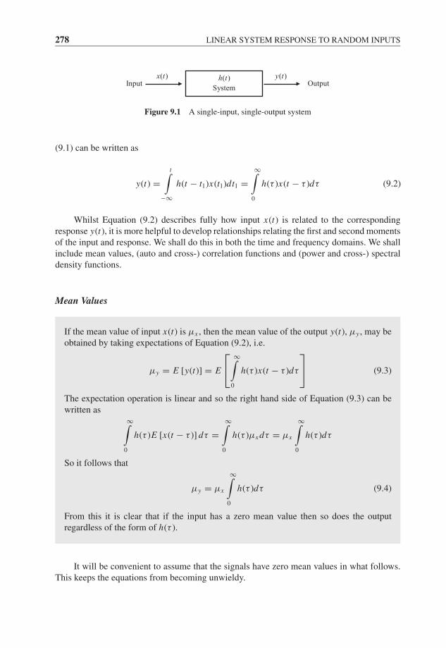
JWBK207-09 JWBK207-Shin January 30, 2008 15:55 Char Count= 0
278 LINEAR SYSTEM RESPONSE TO RANDOM INPUTS
( )x t ( )
System
h tOutput
( )y tInput
Figure 9.1 A single-input, single-output system
(9.1) can be written as
y(t) =t∫
−∞h(t − t1)x(t1)dt1 =
∞∫0
h(τ )x(t − τ )dτ (9.2)
Whilst Equation (9.2) describes fully how input x(t) is related to the correspondingresponse y(t), it is more helpful to develop relationships relating the first and second momentsof the input and response. We shall do this in both the time and frequency domains. We shallinclude mean values, (auto and cross-) correlation functions and (power and cross-) spectraldensity functions.
Mean Values
If the mean value of input x(t) is μx , then the mean value of the output y(t), μy , may beobtained by taking expectations of Equation (9.2), i.e.
μy = E [y(t)] = E
⎡⎣ ∞∫0
h(τ )x(t − τ )dτ
⎤⎦ (9.3)
The expectation operation is linear and so the right hand side of Equation (9.3) can bewritten as
∞∫0
h(τ )E [x(t − τ )] dτ =∞∫
0
h(τ )μx dτ = μx
∞∫0
h(τ )dτ
So it follows that
μy = μx
∞∫0
h(τ )dτ (9.4)
From this it is clear that if the input has a zero mean value then so does the outputregardless of the form of h(τ ).
It will be convenient to assume that the signals have zero mean values in what follows.This keeps the equations from becoming unwieldy.

JWBK207-09 JWBK207-Shin January 30, 2008 15:55 Char Count= 0
SINGLE-INPUT, SINGLE-OUTPUT SYSTEMS 279
Autocorrelation Functions
If x(t) is characterized by its autocorrelation function Rxx (τ ) it is logical to ask how theoutput autocorrelation Ryy(τ ) is related to the Rxx (τ ). So we need to evaluate Ryy(τ ) =E[y(t)y(t + τ )], where y(t) is given by Equation (9.2). This follows, where again weexploit the linear nature of the expected value operator which allows it under integraloperations:
Ryy(τ ) = E[y(t)y(t + τ )] = E
⎡⎣ ∞∫0
∞∫0
h(τ1)x(t − τ1)h(τ2)x(t + τ − τ2)dτ1dτ2
⎤⎦=
∞∫0
∞∫0
h(τ1)h(τ2)E [x(t − τ1)x(t + τ − τ2)]dτ1dτ2 (9.5)
Thus,
Ryy(τ ) =∞∫
0
∞∫0
h(τ1)h(τ2)Rxx (τ + τ1 − τ2)dτ1dτ2 (9.6)
This is rather complicated and is a difficult equation to evaluate, and we find that the frequencydomain equivalent is more useful.
Taking the Fourier transform of Equation (9.6) gives
Syy( f ) =∞∫
−∞Ryy(τ )e− j2π f τ dτ
=∞∫
0
h(τ1)e j2π f τ1 dτ1
∞∫0
h(τ2)e− j2π f τ2 dτ2
∞∫−∞
Rxx (τ + τ1 − τ2)e− j2π f (τ+τ1−τ2)dτ
(9.7)
Let τ + τ1 − τ2 = u in the last integral to yield
Syy( f ) = |H ( f )|2 Sxx ( f ) (9.8)
where H ( f ) = ∫ ∞0
h(τ )e− j2π f τ dτ is the system frequency response function. (Recall thatthe Fourier transform of the convolution of two functions is the product of their transforms,i.e. Y ( f ) = F{y(t)} = F{h(t) ∗ x(t)} = H ( f )X ( f ) which gives |Y ( f )|2 = |H ( f )|2 |X ( f )|2,and compare this with above equation.)
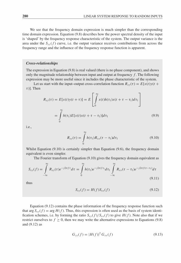
JWBK207-09 JWBK207-Shin January 30, 2008 15:55 Char Count= 0
280 LINEAR SYSTEM RESPONSE TO RANDOM INPUTS
We see that the frequency domain expression is much simpler than the correspondingtime domain expression. Equation (9.8) describes how the power spectral density of the inputis ‘shaped’ by the frequency response characteristic of the system. The output variance is thearea under the Syy( f ) curve, i.e. the output variance receives contributions from across thefrequency range and the influence of the frequency response function is apparent.
Cross-relationships
The expression in Equation (9.8) is real valued (there is no phase component), and showsonly the magnitude relationship between input and output at frequency f . The followingexpression may be more useful since it includes the phase characteristic of the system.
Let us start with the input–output cross-correlation function Rxy(τ ) = E[x(t)y(t +τ )]. Then
Rxy(τ ) = E[x(t)y(t + τ )] = E
⎡⎣ ∞∫0
x(t)h(τ1)x(t + τ − τ1)dτ1
⎤⎦=
∞∫0
h(τ1)E[x(t)x(t + τ − τ1)]dτ1 (9.9)
i.e.,
Rxy(τ ) =∞∫
0
h(τ1)Rxx (τ − τ1)dτ1 (9.10)
Whilst Equation (9.10) is certainly simpler than Equation (9.6), the frequency domainequivalent is even simpler.
The Fourier transform of Equation (9.10) gives the frequency domain equivalent as
Sxy( f ) =∞∫
−∞Rxy(τ )e− j2π f τ dτ =
∞∫0
h(τ1)e− j2π f τ1 dτ1
∞∫−∞
Rxx (τ − τ1)e− j2π f (τ−τ1)dτ
(9.11)thus
Sxy( f ) = H ( f )Sxx ( f ) (9.12)
Equation (9.12) contains the phase information of the frequency response function suchthat arg Sxy( f ) = arg H ( f ). Thus, this expression is often used as the basis of system identi-fication schemes, i.e. by forming the ratio Sxy( f )/Sxx ( f ) to give H ( f ). Note also that if werestrict ourselves to f ≥ 0, then we may write the alternative expressions to Equations (9.8)and (9.12) as
G yy( f ) = |H ( f )|2 Gxx ( f ) (9.13)
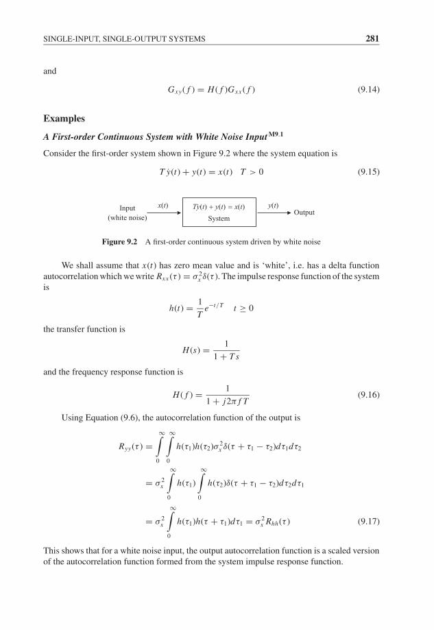
JWBK207-09 JWBK207-Shin January 30, 2008 15:55 Char Count= 0
SINGLE-INPUT, SINGLE-OUTPUT SYSTEMS 281
and
Gxy( f ) = H ( f )Gxx ( f ) (9.14)
Examples
A First-order Continuous System with White Noise Input M9.1
Consider the first-order system shown in Figure 9.2 where the system equation is
T y(t) + y(t) = x(t) T > 0 (9.15)
x(t)
System
Ty(t) y(t) x(t)Output
y(t)Input
(white noise)
Figure 9.2 A first-order continuous system driven by white noise
We shall assume that x(t) has zero mean value and is ‘white’, i.e. has a delta functionautocorrelation which we write Rxx (τ ) = σ 2
x δ(τ ). The impulse response function of the systemis
h(t) = 1
Te−t/T t ≥ 0
the transfer function is
H (s) = 1
1 + T s
and the frequency response function is
H ( f ) = 1
1 + j2π f T(9.16)
Using Equation (9.6), the autocorrelation function of the output is
Ryy(τ ) =∞∫
0
∞∫0
h(τ1)h(τ2)σ 2x δ(τ + τ1 − τ2)dτ1dτ2
= σ 2x
∞∫0
h(τ1)
∞∫0
h(τ2)δ(τ + τ1 − τ2)dτ2dτ1
= σ 2x
∞∫0
h(τ1)h(τ + τ1)dτ1 = σ 2x Rhh(τ ) (9.17)
This shows that for a white noise input, the output autocorrelation function is a scaled versionof the autocorrelation function formed from the system impulse response function.
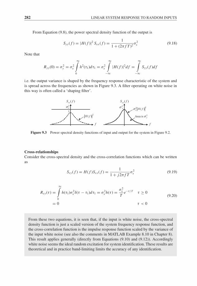
JWBK207-09 JWBK207-Shin January 30, 2008 15:55 Char Count= 0
282 LINEAR SYSTEM RESPONSE TO RANDOM INPUTS
From Equation (9.8), the power spectral density function of the output is
Syy( f ) = |H ( f )|2 Sxx ( f ) = 1
1 + (2π f T )2σ 2
x (9.18)
Note that
Ryy(0) = σ 2y = σ 2
x
∞∫0
h2(τ1)dτ1 = σ 2x
∞∫−∞
|H ( f )|2d f =∞∫
−∞Syy( f )d f
i.e. the output variance is shaped by the frequency response characteristic of the system andis spread across the frequencies as shown in Figure 9.3. A filter operating on white noise inthis way is often called a ‘shaping filter’.
2xσ
( )xxS f
2( )H f
1
( )yyS f
2Area is yσ
22 ( )x H fσ2xσ
ff
Figure 9.3 Power spectral density functions of input and output for the system in Figure 9.2.
Cross-relationshipsConsider the cross-spectral density and the cross-correlation functions which can be writtenas
Sxy( f ) = H ( f )Sxx ( f ) = 1
1 + j2π f Tσ 2
x (9.19)
Rxy(τ ) =∞∫
0
h(τ1)σ 2x δ(τ − τ1)dτ1 = σ 2
x h(τ ) = σ 2x
Te−τ/T τ ≥ 0
= 0 τ < 0
(9.20)
From these two equations, it is seen that, if the input is white noise, the cross-spectraldensity function is just a scaled version of the system frequency response function, andthe cross-correlation function is the impulse response function scaled by the variance ofthe input white noise (see also the comments in MATLAB Example 8.10 in Chapter 8).This result applies generally (directly from Equations (9.10) and (9.12)). Accordinglywhite noise seems the ideal random excitation for system identification. These results aretheoretical and in practice band-limiting limits the accuracy of any identification.
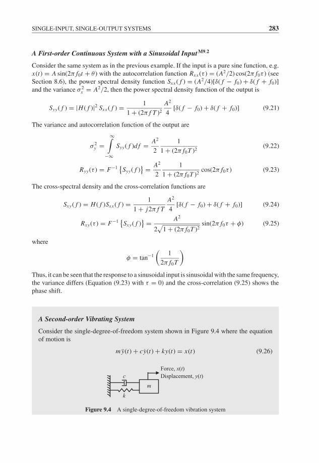
JWBK207-09 JWBK207-Shin January 30, 2008 15:55 Char Count= 0
SINGLE-INPUT, SINGLE-OUTPUT SYSTEMS 283
A First-order Continuous System with a Sinusoidal Input M9.2
Consider the same system as in the previous example. If the input is a pure sine function, e.g.x(t) = A sin(2π f0t + θ ) with the autocorrelation function Rxx (τ ) = (A2/2) cos(2π f0τ ) (seeSection 8.6), the power spectral density function Sxx ( f ) = (A2/4)[δ( f − f0) + δ( f + f0)]and the variance σ 2
x = A2/2, then the power spectral density function of the output is
Syy( f ) = |H ( f )|2 Sxx ( f ) = 1
1 + (2π f T )2
A2
4[δ( f − f0) + δ( f + f0)] (9.21)
The variance and autocorrelation function of the output are
σ 2y =
∞∫−∞
Syy( f )d f = A2
2
1
1 + (2π f0T )2(9.22)
Ryy(τ ) = F−1{
Syy( f )} = A2
2
1
1 + (2π f0T )2cos(2π f0τ ) (9.23)
The cross-spectral density and the cross-correlation functions are
Sxy( f ) = H ( f )Sxx ( f ) = 1
1 + j2π f T
A2
4[δ( f − f0) + δ( f + f0)] (9.24)
Rxy(τ ) = F−1{
Sxy( f )} = A2
2√
1 + (2π f0T )2sin(2π f0τ + φ) (9.25)
where
φ = tan−1
(1
2π f0T
)Thus, it can be seen that the response to a sinusoidal input is sinusoidal with the same frequency,the variance differs (Equation (9.23) with τ = 0) and the cross-correlation (9.25) shows thephase shift.
A Second-order Vibrating System
Consider the single-degree-of-freedom system shown in Figure 9.4 where the equationof motion is
my(t) + cy(t) + ky(t) = x(t) (9.26)
Force, x(t)Displacement, y(t)
m
k
c
Figure 9.4 A single-degree-of-freedom vibration system
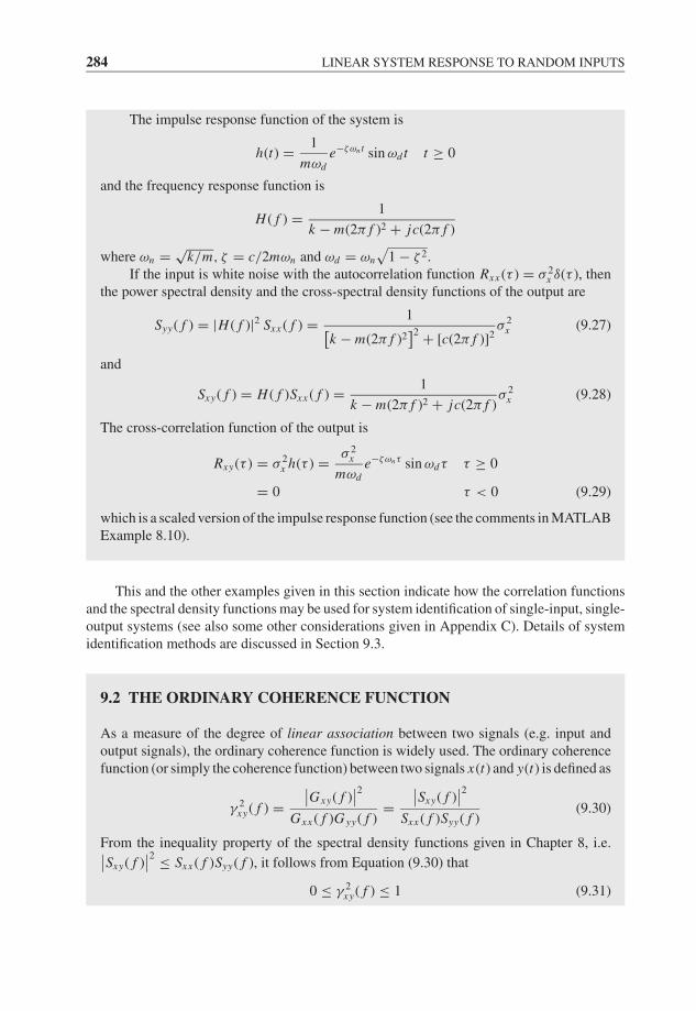
JWBK207-09 JWBK207-Shin January 30, 2008 15:55 Char Count= 0
284 LINEAR SYSTEM RESPONSE TO RANDOM INPUTS
The impulse response function of the system is
h(t) = 1
mωde−ζωn t sin ωd t t ≥ 0
and the frequency response function is
H ( f ) = 1
k − m(2π f )2 + jc(2π f )
where ωn = √k/m, ζ = c/2mωn and ωd = ωn
√1 − ζ 2.
If the input is white noise with the autocorrelation function Rxx (τ ) = σ 2x δ(τ ), then
the power spectral density and the cross-spectral density functions of the output are
Syy( f ) = |H ( f )|2 Sxx ( f ) = 1[k − m(2π f )2
]2 + [c(2π f )]2σ 2
x (9.27)
and
Sxy( f ) = H ( f )Sxx ( f ) = 1
k − m(2π f )2 + jc(2π f )σ 2
x (9.28)
The cross-correlation function of the output is
Rxy(τ ) = σ 2x h(τ ) = σ 2
x
mωde−ζωnτ sin ωdτ τ ≥ 0
= 0 τ < 0 (9.29)
which is a scaled version of the impulse response function (see the comments in MATLABExample 8.10).
This and the other examples given in this section indicate how the correlation functionsand the spectral density functions may be used for system identification of single-input, single-output systems (see also some other considerations given in Appendix C). Details of systemidentification methods are discussed in Section 9.3.
9.2 THE ORDINARY COHERENCE FUNCTION
As a measure of the degree of linear association between two signals (e.g. input andoutput signals), the ordinary coherence function is widely used. The ordinary coherencefunction (or simply the coherence function) between two signals x(t) and y(t) is defined as
γ 2xy( f ) =
∣∣Gxy( f )∣∣2
Gxx ( f )G yy( f )=
∣∣Sxy( f )∣∣2
Sxx ( f )Syy( f )(9.30)
From the inequality property of the spectral density functions given in Chapter 8, i.e.∣∣Sxy( f )∣∣2 ≤ Sxx ( f )Syy( f ), it follows from Equation (9.30) that
0 ≤ γ 2xy( f ) ≤ 1 (9.31)

JWBK207-09 JWBK207-Shin January 30, 2008 15:55 Char Count= 0
THE ORDINARY COHERENCE FUNCTION 285
If x(t) and y(t) are input and output signals, then Syy( f ) = |H ( f )|2 Sxx ( f ) andSxy( f ) = H ( f )Sxx ( f ). So the coherence function for the single-input, single-output sys-tem given in Figure 9.1 is shown to be
γ 2xy( f ) = |H ( f )|2 S2
xx
Sxx ( f ) |H ( f )|2 Sxx ( f )= 1 (9.32)
Thus, it is shown that the coherence function is unity if x(t) and y(t) are linearly related.Conversely, if Sxy( f ) is zero, i.e. the two signals are uncorrelated, then the coherencefunction is zero. If the coherence function is greater than zero but less than one, thenx(t) and y(t) are partially linearly related. Possible departures from linear relationshipbetween x(t) and y(t) include:
1. Noise may be present in the measurements of either or both x(t) and y(t).2. x(t) and y(t) are not only linearly related (e.g. they may also be related nonlinearly).3. y(t) is an output due not only to input x(t) but also to other inputs.
Since γ 2xy( f ) is a function of frequency its appearance across the frequency range can be
very revealing. In some ranges it may be close to unity and in others not, e.g. see Figure9.5, indicating frequency ranges where ‘linearity’ may be more or less evident.
2 ( )xy f
1.0
f
Figure 9.5 A typical example of the coherence function
Effect of Measurement Noise
Case (a) Output NoiseConsider the effect of measurement noise on the output as shown in Figure 9.6, where ym(t) isa measured signal such that ym(t) = y(t) + ny(t). We assume that input x(t) and measurementnoise ny(t) are uncorrelated. Since y(t) is linearly related to x(t), then y(t) and ny(t) are alsouncorrelated. Then, the coherence function between x(t) and ym(t) is
γ 2xym
( f ) =∣∣Sxym ( f )
∣∣2
Sxx ( f )Sym ym ( f )(9.33)
( )x t
( ), noiseyn t
( )my t( )h t( )y t
Figure 9.6 The effect of measurement noise on the output
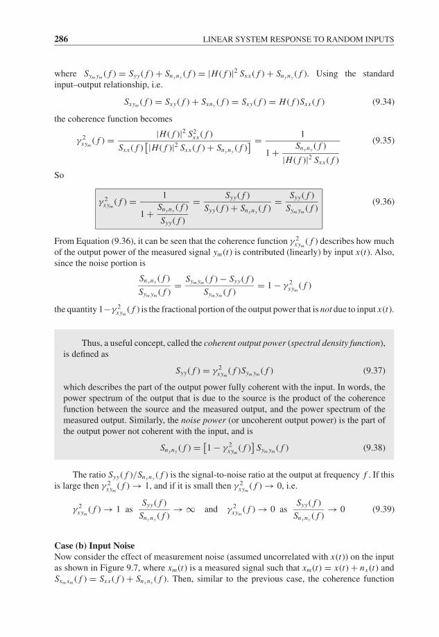
JWBK207-09 JWBK207-Shin January 30, 2008 15:55 Char Count= 0
286 LINEAR SYSTEM RESPONSE TO RANDOM INPUTS
where Sym ym ( f ) = Syy( f ) + Sny ny ( f ) = |H ( f )|2 Sxx ( f ) + Sny ny ( f ). Using the standardinput–output relationship, i.e.
Sxym ( f ) = Sxy( f ) + Sxny ( f ) = Sxy( f ) = H ( f )Sxx ( f ) (9.34)
the coherence function becomes
γ 2xym
( f ) = |H ( f )|2 S2xx ( f )
Sxx ( f )[|H ( f )|2 Sxx ( f ) + Sny ny ( f )
] = 1
1 + Sny ny ( f )
|H ( f )|2 Sxx ( f )
(9.35)
So
γ 2xym
( f ) = 1
1 + Sny ny ( f )
Syy( f )
= Syy( f )
Syy( f ) + Sny ny ( f )= Syy( f )
Sym ym ( f )(9.36)
From Equation (9.36), it can be seen that the coherence function γ 2xym
( f ) describes how muchof the output power of the measured signal ym(t) is contributed (linearly) by input x(t). Also,since the noise portion is
Sny ny ( f )
Sym ym ( f )= Sym ym ( f ) − Syy( f )
Sym ym ( f )= 1 − γ 2
xym( f )
the quantity 1−γ 2xym
( f ) is the fractional portion of the output power that is not due to input x(t).
Thus, a useful concept, called the coherent output power (spectral density function),is defined as
Syy( f ) = γ 2xym
( f )Sym ym ( f ) (9.37)
which describes the part of the output power fully coherent with the input. In words, thepower spectrum of the output that is due to the source is the product of the coherencefunction between the source and the measured output, and the power spectrum of themeasured output. Similarly, the noise power (or uncoherent output power) is the part ofthe output power not coherent with the input, and is
Sny ny ( f ) = [1 − γ 2
xym( f )
]Sym ym ( f ) (9.38)
The ratio Syy( f )/Sny ny ( f ) is the signal-to-noise ratio at the output at frequency f . If thisis large then γ 2
xym( f ) → 1, and if it is small then γ 2
xym( f ) → 0, i.e.
γ 2xym
( f ) → 1 asSyy( f )
Sny ny ( f )→ ∞ and γ 2
xym( f ) → 0 as
Syy( f )
Sny ny ( f )→ 0 (9.39)
Case (b) Input NoiseNow consider the effect of measurement noise (assumed uncorrelated with x(t)) on the inputas shown in Figure 9.7, where xm(t) is a measured signal such that xm(t) = x(t) + nx (t) andSxm xm ( f ) = Sxx ( f ) + Snx nx ( f ). Then, similar to the previous case, the coherence function

JWBK207-09 JWBK207-Shin January 30, 2008 15:55 Char Count= 0
SYSTEM IDENTIFICATION 287
( )x t ( )y t
( )xn t
( )mx t
+
( )h t
Figure 9.7 The effect of measurement noise on the input
between xm(t) and y(t) is
γ 2xm y( f ) = 1
1 + Snx nx ( f )
Sxx ( f )
= Sxx ( f )
Sxx ( f ) + Snx nx ( f )= Sxx ( f )
Sxm xm ( f )(9.40)
Thus, the input power and noise power can be decomposed as
Sxx ( f ) = γ 2xm y( f )Sxm xm ( f ) (9.41)
and
Snx nx ( f ) = [1 − γ 2
xm y( f )]
Sxm xm ( f ) (9.42)
Case (c) Input and Output NoiseConsider the uncorrelated noise at both input and output as shown in Figure 9.8, where xm(t)and ym(t) are the measured input and output.
( )x t ( )y t
( )yn t( )xn t
( )my t( )mx t
( )h t
Figure 9.8 The effect of measurement noise on both input and output
The noises are assumed mutually uncorrelated and uncorrelated with x(t). Then the coherencefunction between xm(t) and ym(t) becomes
γ 2xm ym
( f ) =∣∣Sxm ym ( f )
∣∣2
Sxm xm ( f )Sym ym ( f )= 1
1 + Snx nx ( f )
Sxx ( f )+ Sny ny ( f )
Syy( f )+ Snx nx ( f )Sny ny ( f )
Sxx ( f )Syy( f )
(9.43)
Note that, in this case, it is not possible to obtain the signal powers Sxx ( f ) and Syy( f )using the measured signals xm(t) and ym(t) without knowledge or measurement of the noise.
Some comments on the ordinary coherence function are given in Appendix D.
9.3 SYSTEM IDENTIFICATIONM9.4, 9.5
The objective of this section is to show how we can estimate the frequency responsefunction of a linear time-invariant system when the input is a stationary random process.
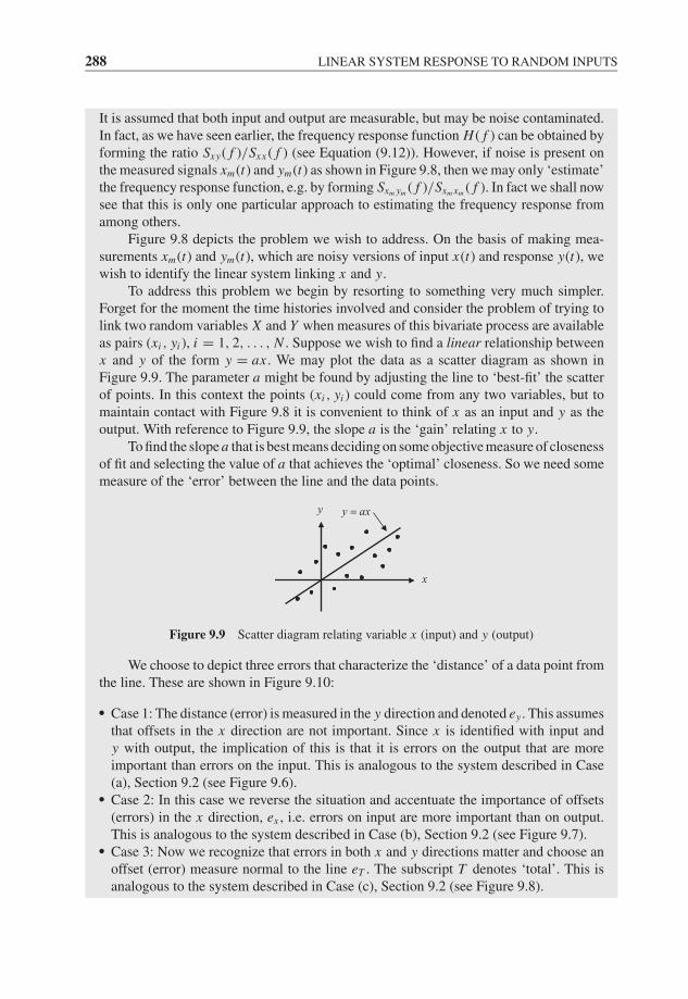
JWBK207-09 JWBK207-Shin January 30, 2008 15:55 Char Count= 0
288 LINEAR SYSTEM RESPONSE TO RANDOM INPUTS
It is assumed that both input and output are measurable, but may be noise contaminated.In fact, as we have seen earlier, the frequency response function H ( f ) can be obtained byforming the ratio Sxy( f )/Sxx ( f ) (see Equation (9.12)). However, if noise is present onthe measured signals xm(t) and ym(t) as shown in Figure 9.8, then we may only ‘estimate’the frequency response function, e.g. by forming Sxm ym ( f )/Sxm xm ( f ). In fact we shall nowsee that this is only one particular approach to estimating the frequency response fromamong others.
Figure 9.8 depicts the problem we wish to address. On the basis of making mea-surements xm(t) and ym(t), which are noisy versions of input x(t) and response y(t), wewish to identify the linear system linking x and y.
To address this problem we begin by resorting to something very much simpler.Forget for the moment the time histories involved and consider the problem of trying tolink two random variables X and Y when measures of this bivariate process are availableas pairs (xi , yi ), i = 1, 2, . . . , N . Suppose we wish to find a linear relationship betweenx and y of the form y = ax . We may plot the data as a scatter diagram as shown inFigure 9.9. The parameter a might be found by adjusting the line to ‘best-fit’ the scatterof points. In this context the points (xi , yi ) could come from any two variables, but tomaintain contact with Figure 9.8 it is convenient to think of x as an input and y as theoutput. With reference to Figure 9.9, the slope a is the ‘gain’ relating x to y.
To find the slope a that is best means deciding on some objective measure of closenessof fit and selecting the value of a that achieves the ‘optimal’ closeness. So we need somemeasure of the ‘error’ between the line and the data points.
y ax
x
y
Figure 9.9 Scatter diagram relating variable x (input) and y (output)
We choose to depict three errors that characterize the ‘distance’ of a data point fromthe line. These are shown in Figure 9.10:� Case 1: The distance (error) is measured in the y direction and denoted ey . This assumes
that offsets in the x direction are not important. Since x is identified with input andy with output, the implication of this is that it is errors on the output that are moreimportant than errors on the input. This is analogous to the system described in Case(a), Section 9.2 (see Figure 9.6).� Case 2: In this case we reverse the situation and accentuate the importance of offsets(errors) in the x direction, ex , i.e. errors on input are more important than on output.This is analogous to the system described in Case (b), Section 9.2 (see Figure 9.7).� Case 3: Now we recognize that errors in both x and y directions matter and choose anoffset (error) measure normal to the line eT . The subscript T denotes ‘total’. This isanalogous to the system described in Case (c), Section 9.2 (see Figure 9.8).
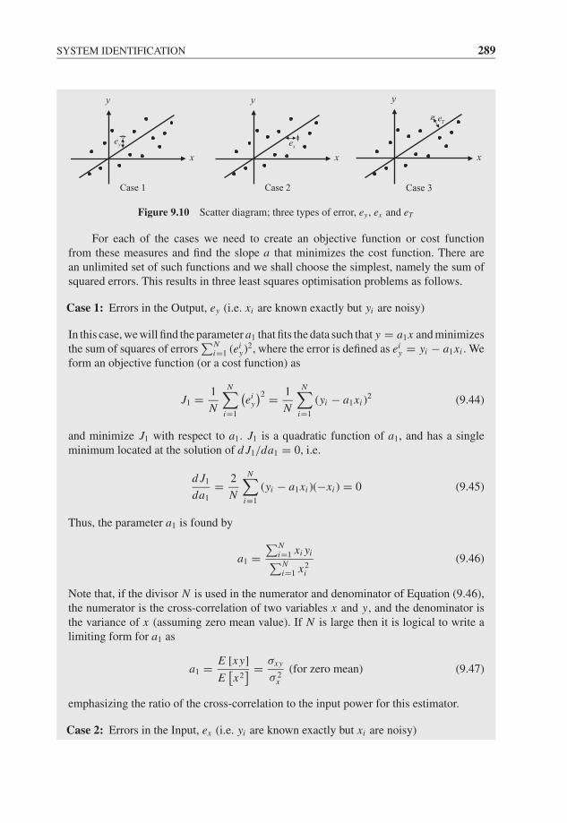
JWBK207-09 JWBK207-Shin January 30, 2008 15:55 Char Count= 0
SYSTEM IDENTIFICATION 289
ye
x
y
Case 1
xe
x
y
Case 2
Te
x
y
Case 3
Figure 9.10 Scatter diagram; three types of error, ey , ex and eT
For each of the cases we need to create an objective function or cost functionfrom these measures and find the slope a that minimizes the cost function. There arean unlimited set of such functions and we shall choose the simplest, namely the sum ofsquared errors. This results in three least squares optimisation problems as follows.
Case 1: Errors in the Output, ey (i.e. xi are known exactly but yi are noisy)
In this case, we will find the parameter a1 that fits the data such that y = a1x and minimizesthe sum of squares of errors
∑Ni=1 (ei
y)2, where the error is defined as eiy = yi − a1xi . We
form an objective function (or a cost function) as
J1 = 1
N
N∑i=1
(ei
y
)2 = 1
N
N∑i=1
(yi − a1xi )2 (9.44)
and minimize J1 with respect to a1. J1 is a quadratic function of a1, and has a singleminimum located at the solution of d J1/da1 = 0, i.e.
d J1
da1
= 2
N
N∑i=1
(yi − a1xi )(−xi ) = 0 (9.45)
Thus, the parameter a1 is found by
a1 =∑N
i=1 xi yi∑Ni=1 x2
i
(9.46)
Note that, if the divisor N is used in the numerator and denominator of Equation (9.46),the numerator is the cross-correlation of two variables x and y, and the denominator isthe variance of x (assuming zero mean value). If N is large then it is logical to write alimiting form for a1 as
a1 = E [xy]
E[x2
] = σxy
σ 2x
(for zero mean) (9.47)
emphasizing the ratio of the cross-correlation to the input power for this estimator.
Case 2: Errors in the Input, ex (i.e. yi are known exactly but xi are noisy)
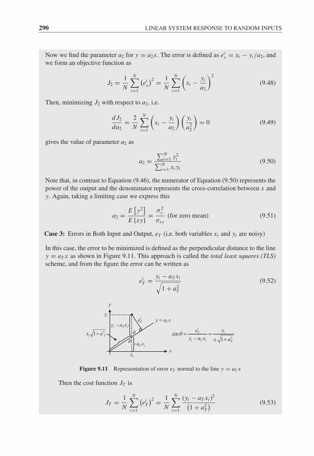
JWBK207-09 JWBK207-Shin January 30, 2008 15:55 Char Count= 0
290 LINEAR SYSTEM RESPONSE TO RANDOM INPUTS
Now we find the parameter a2 for y = a2x . The error is defined as eix = xi − yi/a2, and
we form an objective function as
J2 = 1
N
N∑i=1
(ei
x
)2 = 1
N
N∑i=1
(xi − yi
a2
)2
(9.48)
Then, minimizing J2 with respect to a2, i.e.
d J2
da2
= 2
N
N∑i=1
(xi − yi
a2
) (yi
a22
)= 0 (9.49)
gives the value of parameter a2 as
a2 =∑N
i=1 y2i∑N
i=1 xi yi
(9.50)
Note that, in contrast to Equation (9.46), the numerator of Equation (9.50) represents thepower of the output and the denominator represents the cross-correlation between x andy. Again, taking a limiting case we express this
a2 = E[y2
]E [xy]
= σ 2y
σxy(for zero mean) (9.51)
Case 3: Errors in Both Input and Output, eT (i.e. both variables xi and yi are noisy)
In this case, the error to be minimized is defined as the perpendicular distance to the liney = aT x as shown in Figure 9.11. This approach is called the total least squares (TLS)scheme, and from the figure the error can be written as
eiT = yi − aT xi√
1 + a2T
(9.52)
Ty a x
ix
iy
T ia x
i T iy a x21i Tx a
2sin
1
iiT
i T i i T
xe
y a x x a
iTe
y
x
Figure 9.11 Representation of error eT normal to the line y = aT x
Then the cost function JT is
JT = 1
N
N∑i=1
(ei
T
)2 = 1
N
N∑i=1
(yi − aT xi )2(
1 + a2T
) (9.53)
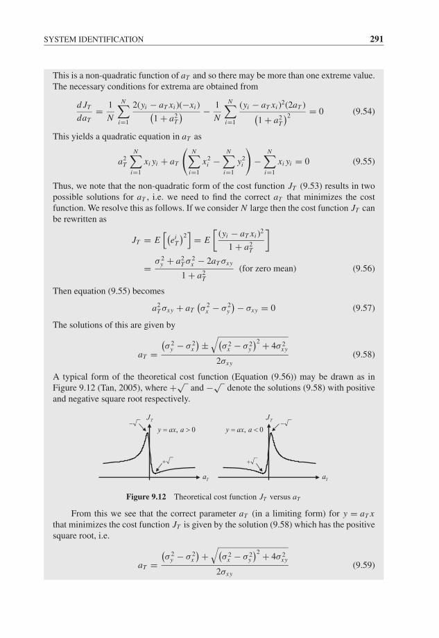
JWBK207-09 JWBK207-Shin January 30, 2008 15:55 Char Count= 0
SYSTEM IDENTIFICATION 291
This is a non-quadratic function of aT and so there may be more than one extreme value.The necessary conditions for extrema are obtained from
d JT
daT= 1
N
N∑i=1
2(yi − aT xi )(−xi )(1 + a2
T
) − 1
N
N∑i=1
(yi − aT xi )2(2aT )(
1 + a2T
)2= 0 (9.54)
This yields a quadratic equation in aT as
a2T
N∑i=1
xi yi + aT
(N∑
i=1
x2i −
N∑i=1
y2i
)−
N∑i=1
xi yi = 0 (9.55)
Thus, we note that the non-quadratic form of the cost function JT (9.53) results in twopossible solutions for aT , i.e. we need to find the correct aT that minimizes the costfunction. We resolve this as follows. If we consider N large then the cost function JT canbe rewritten as
JT = E[(
eiT
)2]
= E
[(yi − aT xi )
2
1 + a2T
]= σ 2
y + a2T σ 2
x − 2aT σxy
1 + a2T
(for zero mean) (9.56)
Then equation (9.55) becomes
a2T σxy + aT
(σ 2
x − σ 2y
) − σxy = 0 (9.57)
The solutions of this are given by
aT =(σ 2
y − σ 2x
) ±√(
σ 2x − σ 2
y
)2 + 4σ 2xy
2σxy(9.58)
A typical form of the theoretical cost function (Equation (9.56)) may be drawn as inFigure 9.12 (Tan, 2005), where +√
and −√denote the solutions (9.58) with positive
and negative square root respectively.
Ta
TJ
, 0y ax a
Ta
TJ
, 0y ax a
Figure 9.12 Theoretical cost function JT versus aT
From this we see that the correct parameter aT (in a limiting form) for y = aT xthat minimizes the cost function JT is given by the solution (9.58) which has the positivesquare root, i.e.
aT =(σ 2
y − σ 2x
) +√(
σ 2x − σ 2
y
)2 + 4σ 2xy
2σxy(9.59)
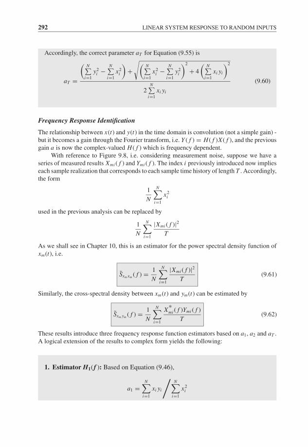
JWBK207-09 JWBK207-Shin January 30, 2008 15:55 Char Count= 0
292 LINEAR SYSTEM RESPONSE TO RANDOM INPUTS
Accordingly, the correct parameter aT for Equation (9.55) is
aT =
(N∑
i=1
y2i −
N∑i=1
x2i
)+
√(N∑
i=1
x2i −
N∑i=1
y2i
)2
+ 4
(N∑
i=1
xi yi
)2
2N∑
i=1
xi yi
(9.60)
Frequency Response Identification
The relationship between x(t) and y(t) in the time domain is convolution (not a simple gain) -but it becomes a gain through the Fourier transform, i.e. Y ( f ) = H ( f )X ( f ), and the previousgain a is now the complex-valued H ( f ) which is frequency dependent.
With reference to Figure 9.8, i.e. considering measurement noise, suppose we have aseries of measured results Xmi ( f ) and Ymi ( f ). The index i previously introduced now implieseach sample realization that corresponds to each sample time history of length T . Accordingly,the form
1
N
N∑i=1
x2i
used in the previous analysis can be replaced by
1
N
N∑i=1
|Xmi ( f )|2T
As we shall see in Chapter 10, this is an estimator for the power spectral density function ofxm(t), i.e.
Sxm xm ( f ) = 1
N
N∑i=1
|Xmi ( f )|2T
(9.61)
Similarly, the cross-spectral density between xm(t) and ym(t) can be estimated by
Sxm ym ( f ) = 1
N
N∑i=1
X*mi ( f )Ymi ( f )
T(9.62)
These results introduce three frequency response function estimators based on a1, a2 and aT .A logical extension of the results to complex form yields the following:
1. Estimator H1(f ): Based on Equation (9.46),
a1 =N∑
i=1
xi yi
/N∑
i=1
x2i
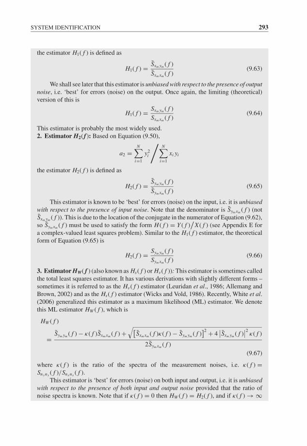
JWBK207-09 JWBK207-Shin January 30, 2008 15:55 Char Count= 0
SYSTEM IDENTIFICATION 293
the estimator H1( f ) is defined as
H1( f ) = Sxm ym ( f )
Sxm xm ( f )(9.63)
We shall see later that this estimator is unbiased with respect to the presence of outputnoise, i.e. ‘best’ for errors (noise) on the output. Once again, the limiting (theoretical)version of this is
H1( f ) = Sxm ym ( f )
Sxm xm ( f )(9.64)
This estimator is probably the most widely used.2. Estimator H2( f ): Based on Equation (9.50),
a2 =N∑
i=1
y2i
/N∑
i=1
xi yi
the estimator H2( f ) is defined as
H2( f ) = Sym ym ( f )
Sym xm ( f )(9.65)
This estimator is known to be ‘best’ for errors (noise) on the input, i.e. it is unbiasedwith respect to the presence of input noise. Note that the denominator is Sym xm ( f ) (notSxm ym ( f )). This is due to the location of the conjugate in the numerator of Equation (9.62),so Sym xm ( f ) must be used to satisfy the form H ( f ) = Y ( f )
/X ( f ) (see Appendix E for
a complex-valued least squares problem). Similar to the H1( f ) estimator, the theoreticalform of Equation (9.65) is
H2( f ) = Sym ym ( f )
Sym xm ( f )(9.66)
3. Estimator HW( f ) (also known as Hs( f ) or Hν( f )): This estimator is sometimes calledthe total least squares estimator. It has various derivations with slightly different forms –sometimes it is referred to as the Hν( f ) estimator (Leuridan et al., 1986; Allemang andBrown, 2002) and as the Hs( f ) estimator (Wicks and Vold, 1986). Recently, White et al.(2006) generalized this estimator as a maximum likelihood (ML) estimator. We denotethis ML estimator HW ( f ), which is
HW ( f )
=Sym ym ( f ) − κ( f )Sxm xm ( f ) +
√[Sxm xm ( f )κ( f ) − Sym ym ( f )
]2 + 4∣∣Sxm ym ( f )
∣∣2κ( f )
2Sym xm ( f )
(9.67)
where κ( f ) is the ratio of the spectra of the measurement noises, i.e. κ( f ) =Sny ny ( f )/Snx nx ( f ).
This estimator is ‘best’ for errors (noise) on both input and output, i.e. it is unbiasedwith respect to the presence of both input and output noise provided that the ratio ofnoise spectra is known. Note that if κ( f ) = 0 then HW ( f ) = H2( f ), and if κ( f ) → ∞
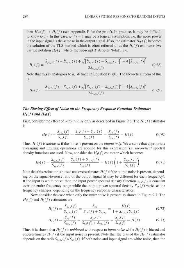
JWBK207-09 JWBK207-Shin January 30, 2008 15:55 Char Count= 0
294 LINEAR SYSTEM RESPONSE TO RANDOM INPUTS
then HW ( f ) → H1( f ) (see Appendix F for the proof). In practice, it may be difficultto know κ( f ). In this case, κ( f ) = 1 may be a logical assumption, i.e. the noise powerin the input signal is the same as in the output signal. If so, the estimator HW ( f ) becomesthe solution of the TLS method which is often referred to as the Hν( f ) estimator (weuse the notation HT ( f ) where the subscript T denotes ‘total’), i.e.
HT ( f ) =Sym ym ( f ) − Sxm xm ( f ) +
√[Sxm xm ( f ) − Sym ym ( f )
]2 + 4∣∣Sxm ym ( f )
∣∣2
2Sym xm ( f )(9.68)
Note that this is analogous to aT defined in Equation (9.60). The theoretical form of thisis
HT ( f ) =Sym ym ( f ) − Sxm xm ( f ) +
√[Sxm xm ( f ) − Sym ym ( f )
]2 + 4∣∣Sxm ym ( f )
∣∣2
2Sym xm ( f )(9.69)
The Biasing Effect of Noise on the Frequency Response Function EstimatorsH1( f ) and H2( f )
First, consider the effect of output noise only as described in Figure 9.6. The H1( f ) estimatoris
H1( f ) = Sxym ( f )
Sxx ( f )= Sxy( f ) + Sxny ( f )
Sxx ( f )= Sxy( f )
Sxx ( f )= H ( f ) (9.70)
Thus, H1( f ) is unbiased if the noise is present on the output only. We assume that appropriateaveraging and limiting operations are applied for this expression, i.e. theoretical spectraldensity functions are used. Now, consider the H2( f ) estimator which becomes
H2( f ) = Sym ym ( f )
Sym x ( f )= Syy( f ) + Sny ny ( f )
Syx ( f )= H ( f )
(1 + Sny ny ( f )
Syy( f )
)(9.71)
Note that this estimator is biased and overestimates H ( f ) if the output noise is present, depend-ing on the signal-to-noise ratio of the output signal (it may be different for each frequency).If the input is white noise, then the input power spectral density function Sxx ( f ) is constantover the entire frequency range while the output power spectral density Syy( f ) varies as thefrequency changes, depending on the frequency response characteristics.
Now consider the case when only the input noise is present as shown in Figure 9.7. TheH1( f ) and H2( f ) estimators are
H1( f ) = Sxm y( f )
Sxm xm ( f )= Sxy
Sxx ( f ) + Snx nx
= H ( f )
1 + Snx nx /Sxx ( f )(9.72)
H2( f ) = Syy( f )
Syxm ( f )= Syy( f )
Syx ( f ) + Synx ( f )= Syy( f )
Syx ( f )= H ( f ) (9.73)
Thus, it is shown that H2( f ) is unbiased with respect to input noise while H1( f ) is biased andunderestimates H ( f ) if the input noise is present. Note that the bias of the H1( f ) estimatordepends on the ratio Snx nx ( f )/Sxx ( f ). If both noise and input signal are white noise, then the
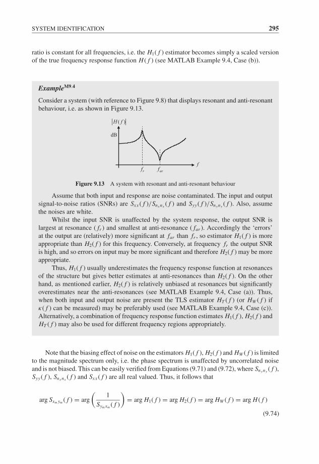
JWBK207-09 JWBK207-Shin January 30, 2008 15:55 Char Count= 0
SYSTEM IDENTIFICATION 295
ratio is constant for all frequencies, i.e. the H1( f ) estimator becomes simply a scaled versionof the true frequency response function H ( f ) (see MATLAB Example 9.4, Case (b)).
ExampleM9.4
Consider a system (with reference to Figure 9.8) that displays resonant and anti-resonantbehaviour, i.e. as shown in Figure 9.13.
farf
( )H f
rf
dB
Figure 9.13 A system with resonant and anti-resonant behaviour
Assume that both input and response are noise contaminated. The input and outputsignal-to-noise ratios (SNRs) are Sxx ( f )/Snx nx ( f ) and Syy( f )/Sny ny ( f ). Also, assumethe noises are white.
Whilst the input SNR is unaffected by the system response, the output SNR islargest at resonance ( fr ) and smallest at anti-resonance ( far ). Accordingly the ‘errors’at the output are (relatively) more significant at far than fr , so estimator H1( f ) is moreappropriate than H2( f ) for this frequency. Conversely, at frequency fr the output SNRis high, and so errors on input may be more significant and therefore H2( f ) may be moreappropriate.
Thus, H1( f ) usually underestimates the frequency response function at resonancesof the structure but gives better estimates at anti-resonances than H2( f ). On the otherhand, as mentioned earlier, H2( f ) is relatively unbiased at resonances but significantlyoverestimates near the anti-resonances (see MATLAB Example 9.4, Case (a)). Thus,when both input and output noise are present the TLS estimator HT ( f ) (or HW ( f ) ifκ( f ) can be measured) may be preferably used (see MATLAB Example 9.4, Case (c)).Alternatively, a combination of frequency response function estimates H1( f ), H2( f ) andHT ( f ) may also be used for different frequency regions appropriately.
Note that the biasing effect of noise on the estimators H1( f ), H2( f ) and HW ( f ) is limitedto the magnitude spectrum only, i.e. the phase spectrum is unaffected by uncorrelated noiseand is not biased. This can be easily verified from Equations (9.71) and (9.72), where Sny ny ( f ),Syy( f ), Snx nx ( f ) and Sxx ( f ) are all real valued. Thus, it follows that
arg Sxm ym ( f ) = arg
(1
Sym xm ( f )
)= arg H1( f ) = arg H2( f ) = arg HW ( f ) = arg H ( f )
(9.74)
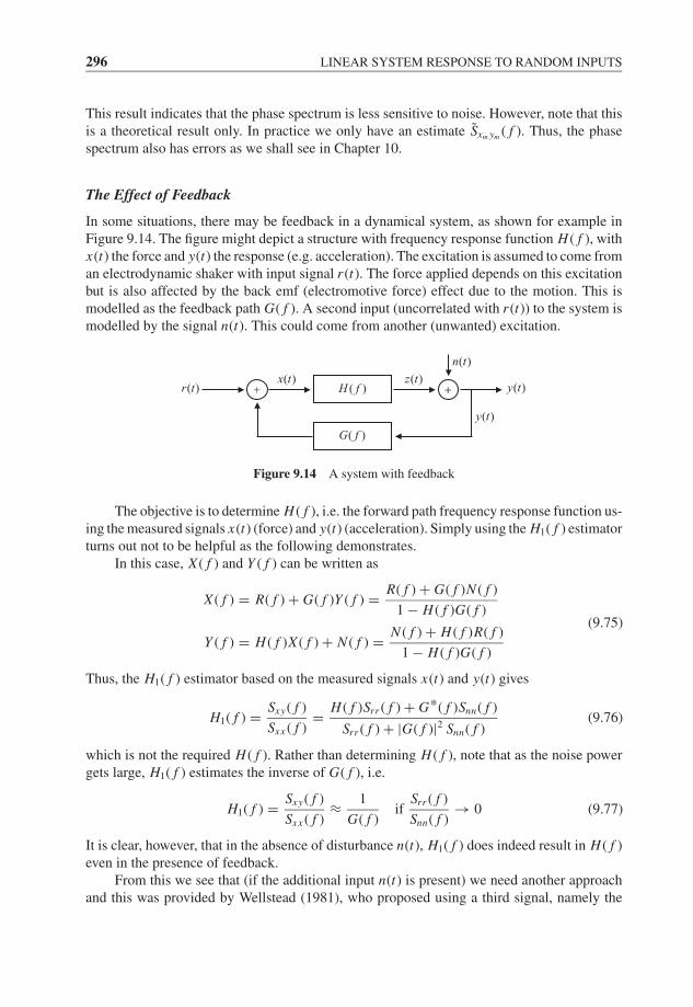
JWBK207-09 JWBK207-Shin January 30, 2008 15:55 Char Count= 0
296 LINEAR SYSTEM RESPONSE TO RANDOM INPUTS
This result indicates that the phase spectrum is less sensitive to noise. However, note that thisis a theoretical result only. In practice we only have an estimate Sxm ym ( f ). Thus, the phasespectrum also has errors as we shall see in Chapter 10.
The Effect of Feedback
In some situations, there may be feedback in a dynamical system, as shown for example inFigure 9.14. The figure might depict a structure with frequency response function H ( f ), withx(t) the force and y(t) the response (e.g. acceleration). The excitation is assumed to come froman electrodynamic shaker with input signal r (t). The force applied depends on this excitationbut is also affected by the back emf (electromotive force) effect due to the motion. This ismodelled as the feedback path G( f ). A second input (uncorrelated with r (t)) to the system ismodelled by the signal n(t). This could come from another (unwanted) excitation.
( )x t
( )n t
( )y t( )H f( )z t
( )G f
( )y t
( )r t
Figure 9.14 A system with feedback
The objective is to determine H ( f ), i.e. the forward path frequency response function us-ing the measured signals x(t) (force) and y(t) (acceleration). Simply using the H1( f ) estimatorturns out not to be helpful as the following demonstrates.
In this case, X ( f ) and Y ( f ) can be written as
X ( f ) = R( f ) + G( f )Y ( f ) = R( f ) + G( f )N ( f )
1 − H ( f )G( f )(9.75)
Y ( f ) = H ( f )X ( f ) + N ( f ) = N ( f ) + H ( f )R( f )
1 − H ( f )G( f )
Thus, the H1( f ) estimator based on the measured signals x(t) and y(t) gives
H1( f ) = Sxy( f )
Sxx ( f )= H ( f )Srr ( f ) + G*( f )Snn( f )
Srr ( f ) + |G( f )|2 Snn( f )(9.76)
which is not the required H ( f ). Rather than determining H ( f ), note that as the noise powergets large, H1( f ) estimates the inverse of G( f ), i.e.
H1( f ) = Sxy( f )
Sxx ( f )≈ 1
G( f )if
Srr ( f )
Snn( f )→ 0 (9.77)
It is clear, however, that in the absence of disturbance n(t), H1( f ) does indeed result in H ( f )even in the presence of feedback.
From this we see that (if the additional input n(t) is present) we need another approachand this was provided by Wellstead (1981), who proposed using a third signal, namely the
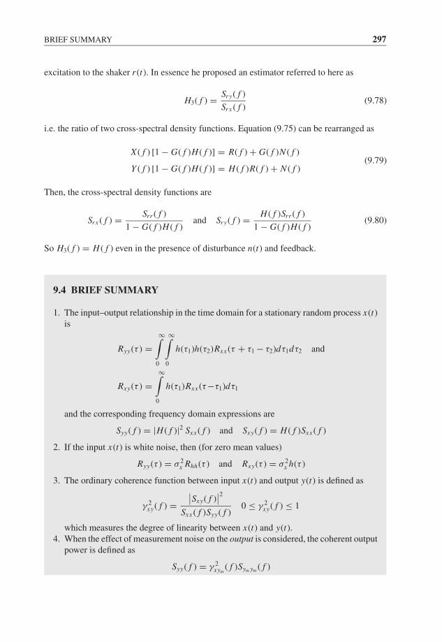
JWBK207-09 JWBK207-Shin January 30, 2008 15:55 Char Count= 0
BRIEF SUMMARY 297
excitation to the shaker r (t). In essence he proposed an estimator referred to here as
H3( f ) = Sry( f )
Sr x ( f )(9.78)
i.e. the ratio of two cross-spectral density functions. Equation (9.75) can be rearranged as
X ( f ) [1 − G( f )H ( f )] = R( f ) + G( f )N ( f )(9.79)
Y ( f ) [1 − G( f )H ( f )] = H ( f )R( f ) + N ( f )
Then, the cross-spectral density functions are
Sr x ( f ) = Srr ( f )
1 − G( f )H ( f )and Sry( f ) = H ( f )Srr ( f )
1 − G( f )H ( f )(9.80)
So H3( f ) = H ( f ) even in the presence of disturbance n(t) and feedback.
9.4 BRIEF SUMMARY
1. The input–output relationship in the time domain for a stationary random process x(t)is
Ryy(τ ) =∞∫
0
∞∫0
h(τ1)h(τ2)Rxx (τ + τ1 − τ2)dτ1dτ2 and
Rxy(τ ) =∞∫
0
h(τ1)Rxx (τ−τ1)dτ1
and the corresponding frequency domain expressions are
Syy( f ) = |H ( f )|2 Sxx ( f ) and Sxy( f ) = H ( f )Sxx ( f )
2. If the input x(t) is white noise, then (for zero mean values)
Ryy(τ ) = σ 2x Rhh(τ ) and Rxy(τ ) = σ 2
x h(τ )
3. The ordinary coherence function between input x(t) and output y(t) is defined as
γ 2xy( f ) =
∣∣Sxy( f )∣∣2
Sxx ( f )Syy( f )0 ≤ γ 2
xy( f ) ≤ 1
which measures the degree of linearity between x(t) and y(t).4. When the effect of measurement noise on the output is considered, the coherent output
power is defined as
Syy( f ) = γ 2xym
( f )Sym ym ( f )

JWBK207-09 JWBK207-Shin January 30, 2008 15:55 Char Count= 0
298 LINEAR SYSTEM RESPONSE TO RANDOM INPUTS
and the noise power (or uncoherent output power) is defined as
Sny ny ( f ) = [1 − γ 2
xym( f )
]Sym ym ( f )
5. Power spectral and cross-spectral density functions can be estimated by
Sxm xm ( f ) = 1
N
N∑i=1
|Xmi ( f )|2T
and Sxm ym ( f ) = 1
N
N∑i=1
X*mi ( f )Ymi ( f )
T
6. The frequency response function is estimated by:
(a) H1( f ) = Sxm ym ( f )
Sxm xm ( f )
which is unbiased with respect to the output noise;
(b) H2( f ) = Sym ym ( f )
Sym xm ( f )
which is unbiased with respect to the input noise;
(c) HW ( f ) =Sym ym ( f ) − κ( f )Sxm xm ( f ) +
√[Sxm xm ( f )κ( f ) − Sym ym ( f )
]2 + 4∣∣Sxm ym ( f )
∣∣2κ( f )
2Sym xm ( f )
where κ( f ) = Sny ny ( f )/Snx nx ( f ). This is unbiased with respect to both input andoutput noise. If κ( f ) is unknown, κ( f ) = 1 may be used.
9.5 MATLAB EXAMPLES
Example 9.1: System identification using spectral density functions: a first-ordersystem
Consider the following first-order system (see Equation (9.15))
T y(t) + y(t) = x(t)
where the impulse response function is h(t) = (1/T )e−t/T and the frequency re-sponse function is H ( f ) = 1/(1 + j2π f T ). In this example, we use the band-limitedwhite noise as an input x(t); then the output y(t) is obtained by the convolution, i.e.y(t) = h(t) ∗ x(t). The spectral density functions Sxx ( f ) and Sxy( f ) are estimated usingWelch’s method (see Chapter 10 for details, and also see Comments 2 in MATLABExample 8.10).
Then, we shall estimate the frequency response function based on Equation (9.12),Sxy( f ) = H ( f )Sxx ( f ), i.e. H1( f ) = Sxy( f )/Sxx ( f ). This estimate will be comparedwith the DFT of h(t) (we mean here the DFT of the sampled, truncated impulse responsefunction).
In this MATLAB example, we do not consider measurement noise. So, we note thatH1( f ) = H2( f ) = HT ( f ).

JWBK207-09 JWBK207-Shin January 30, 2008 15:55 Char Count= 0
MATLAB EXAMPLES 299
Line MATLAB code Comments
12
34
clear allfs=500; T1=1; T2=40; t1=0:1/fs:T1;t2=0:1/fs:T2-1/fs;T=0.1;h=1/T*exp(-t1/T);
Define sampling rate and time variables t1(for the impulse response function h(t)) andt2 (for the band-limited white noise inputx(t)). Then, generate the impulse responsesequence accordingly which is truncated at1 second.
56789
10
11
randn('state',0);x=randn(1,T2*fs);fc=30; [b, a] = butter(9,fc/(fs/2));x=filter(b,a,x);x=x-mean(x); x=x/std(x);y=conv(h,x); y=y(1:end-length(h)+1);% or y=filter(h,1,x);y=y/fs;
Generate the band-limited white noise inputsignal x(t). The cut-off frequency is set to30 Hz for this example. The input sequencehas a zero mean value, and the variance isone.Then, obtain the output sequence by aconvolution operation. Note that the outputsequence y is scaled by the sampling rate inorder to match its corresponding continuousfunction.
1213
14
15
16
17
N=4*fs; % N=10*fs;Sxx=cpsd(x,x, hanning(N),N/2, N, fs,'twosided');Syy=cpsd(y,y, hanning(N),N/2, N, fs,'twosided');Sxy=cpsd(x,y, hanning(N),N/2, N, fs,'twosided');Sxx=fftshift(Sxx); Syy=fftshift(Syy);Sxy=fftshift(Sxy);f=fs*(-N/2:N/2-1)/N;
Calculate the spectral density functionsusing Welch’s method; we use a Hannwindow and 50 % overlap. The length ofsegment is defined by N, and is 4 secondslong in this case.Note that we defined both negative andpositive frequencies (Line 17), thus theMATLAB function ‘fftshift’ is used to shiftthe zero-frequency component to the centreof spectrum.
181920
H1=Sxy./Sxx;H=fftshift(fft(h,N))/fs;Gamma=abs(Sxy).ˆ2./(Sxx.*Syy);
Calculate H1( f ) = Sxy( f )/Sxx ( f ), and alsocalculate H ( f ) using the DFT of the impulseresponse sequence. Also, compute thecoherence function.
212223
24252627
28
figure(1)plot(f, 10*log10(Sxx))xlabel('Frequency (Hz)');ylabel('\itS x x(\itf\rm) (dB)')axis([-30 30 -35 -5])figure(2)plot(f, 10*log10(abs(Sxy)))xlabel('Frequency (Hz)');ylabel('|\itS x y(\itf\rm)| (dB)')axis([-30 30 -35 -15])
Plot the ‘calculated (estimated)’ powerspectral density function and the magnitudespectrum of cross-spectral density function,for the frequency range −30 to 30 Hz.Note that these functions are only estimatesof true spectral density functions, i.e. theyare Sxx ( f ) and Sxy( f ). So, we may see somevariability as shown in the figures. Note thatwe use ‘10*log10(Sxx)’ and‘10*log10(abs(Sxy))’ for dB scale, since thequantities are already power-like.
293031
3233
figure(3)plot(f, 20*log10(abs(H1))); hold onxlabel('Frequency (Hz)');ylabel('|\itH\rm 1(\itf\rm)| (dB)')plot(f, 20*log10(abs(H)), 'r:'); hold offaxis([-30 30 -30 5])
Plot the magnitude spectrum of both H1( f )and H ( f ) for the frequency range −30 to30 Hz.
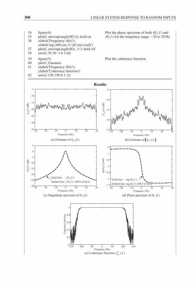
JWBK207-09 JWBK207-Shin January 30, 2008 15:55 Char Count= 0
300 LINEAR SYSTEM RESPONSE TO RANDOM INPUTS
343536
3738
figure(4)plot(f, unwrap(angle(H1))); hold onxlabel('Frequency (Hz)');ylabel('arg\itH\rm 1(\itf\rm) (rad)')plot(f, unwrap(angle(H)), 'r:'); hold offaxis([-30 30 -1.6 1.6])
Plot the phase spectrum of both H1( f ) andH ( f ) for the frequency range −30 to 30 Hz.
394041
42
figure(5)plot(f, Gamma)xlabel('Frequency (Hz)');ylabel('Coherence function')axis([-150 150 0 1.1])
Plot the coherence function.
Results
–30 –20 –10 0 10 20 30–35
–30
–25
–20
–15
–10
–5
Frequency (Hz)
S xx(
f)(d
B)
–30 –20 –10 0 10 20 30–35
–30
–25
–20
–15
Frequency (Hz)
| Sxy
(f)|
(dB
)
(a) Estimate of Sxx (f ) (b) Estimate of Sxy ( f )
(c) Magnitude spectrum of H1 (f ) (d) Phase spectrum of H1 (f )
–30 –20 –10 0 10 20 30–30
–25
–20
–15
–10
–5
0
5
Frequency (Hz)
|H1(f
)|(d
B)
1Solid line: | ( ) |
Dashed line: | ( ) | (DFT of ( ))
H f
H f h t
–30 –20 –10 0 10 20 30–1.5
–1
–0.5
0
0.5
1
1.5
Frequency (Hz)
arg
H1(
f) (
rad
)
1Solid line: arg ( )
Dashed line: arg ( ) (DFT of ( ))
H f
H f h t
–150 –100 –50 0 50 100 1500
0.2
0.4
0.6
0.8
1
Frequency (Hz)
(e) Coherence function γ2xy ( f )
Coher
ence
funct
ion

JWBK207-09 JWBK207-Shin January 30, 2008 15:55 Char Count= 0
MATLAB EXAMPLES 301
Comments:
1. Note that the coherence function γ 2xy( f ) ≈ 1 within the frequency band of interest,
except at the peak (i.e. at zero frequency). The drop of coherence function at f = 0 isdue to the bias error. This bias error can be reduced by improving the resolution (seeChapter 10 for details). To improve the resolution, the length of the segment must beincreased (but note that this reduces the number of averages). For example, replace thenumber 4 with 10 in Line 12 of the MATLAB code. This increases the window lengthin the time domain, thus increasing the frequency resolution. The result is shown inFigure (f), where the coherence function is almost unity including the value at f = 0.
–150 –100 –50 0 50 100 1500
0.2
0.4
0.6
0.8
1
Frequency (Hz)
(f ) Coherence function γ2xy ( f ) using segments
10 seconds long
Coher
ence
funct
ion
2. From Figures (c) and (d), we see that we have an almost perfect estimate for thefrequency response function from H1( f )=Sxy( f )/Sxx ( f ). However, the individualspectral density function estimates show a large variability as shown in Figures (a)and (b). Note that, in theory, Sxx ( f ) is constant and Sxy( f ) is a scaled version of H ( f )if the input is white noise.
It is emphasized that the errors are not due to the noise (we did not considermeasurement noise in this example). In fact, these are the statistical errors inherent inthe estimation processes (see Chapter 10). By comparing Figures (a)–(c), we may seethat the estimate of H ( f ) is less sensitive to the statistical errors than the estimates ofspectral density functions. This will be discussed in Chapter 10.
Note that, even if there is no noise, the estimate of H ( f ) may have large statisticalerrors if the number of averages (for the segment averaging method) is small. Todemonstrate this, change the length of time (T2) in Line 2 of the MATLAB code, i.e.let T2 = 6. The result is shown in Figure (g), where we see relatively large randomerrors near the peak.
–30 –20 –10 0 10 20 30–30
–25
–20
–15
–10
–5
0
5
Frequency (Hz)
|H1(f
)|(d
B)
(g) Magnitude spectrum of H1( f ), for T2 = 6
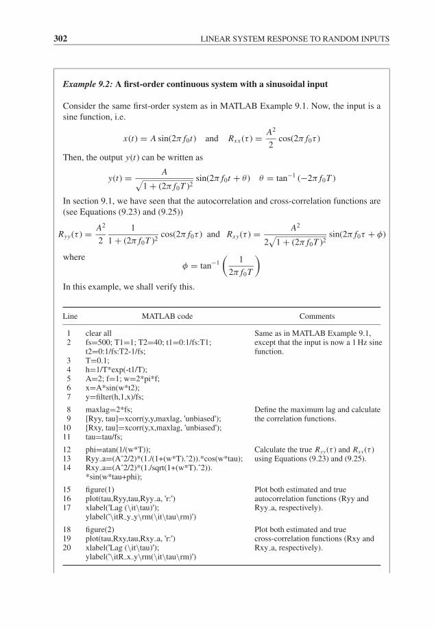
JWBK207-09 JWBK207-Shin January 30, 2008 15:55 Char Count= 0
302 LINEAR SYSTEM RESPONSE TO RANDOM INPUTS
Example 9.2: A first-order continuous system with a sinusoidal input
Consider the same first-order system as in MATLAB Example 9.1. Now, the input is asine function, i.e.
x(t) = A sin(2π f0t) and Rxx (τ ) = A2
2cos(2π f0τ )
Then, the output y(t) can be written as
y(t) = A√1 + (2π f0T )2
sin(2π f0t + θ ) θ = tan−1 (−2π f0T )
In section 9.1, we have seen that the autocorrelation and cross-correlation functions are(see Equations (9.23) and (9.25))
Ryy(τ ) = A2
2
1
1 + (2π f0T )2cos(2π f0τ ) and Rxy(τ ) = A2
2√
1 + (2π f0T )2sin(2π f0τ + φ)
whereφ = tan−1
(1
2π f0T
)In this example, we shall verify this.
Line MATLAB code Comments
12
34567
clear allfs=500; T1=1; T2=40; t1=0:1/fs:T1;t2=0:1/fs:T2-1/fs;T=0.1;h=1/T*exp(-t1/T);A=2; f=1; w=2*pi*f;x=A*sin(w*t2);y=filter(h,1,x)/fs;
Same as in MATLAB Example 9.1,except that the input is now a 1 Hz sinefunction.
89
1011
maxlag=2*fs;[Ryy, tau]=xcorr(y,y,maxlag, 'unbiased');[Rxy, tau]=xcorr(y,x,maxlag, 'unbiased');tau=tau/fs;
Define the maximum lag and calculatethe correlation functions.
121314
phi=atan(1/(w*T));Ryy a=(Aˆ2/2)*(1./(1+(w*T).ˆ2)).*cos(w*tau);Rxy a=(Aˆ2/2)*(1./sqrt(1+(w*T).ˆ2)).*sin(w*tau+phi);
Calculate the true Ryy(τ ) and Rxy(τ )using Equations (9.23) and (9.25).
151617
figure(1)plot(tau,Ryy,tau,Ryy a, 'r:')xlabel('Lag (\it\tau)');ylabel('\itR y y\rm(\it\tau\rm)')
Plot both estimated and trueautocorrelation functions (Ryy andRyy a, respectively).
181920
figure(2)plot(tau,Rxy,tau,Rxy a, 'r:')xlabel('Lag (\it\tau)');ylabel('\itR x y\rm(\it\tau\rm)')
Plot both estimated and truecross-correlation functions (Rxy andRxy a, respectively).
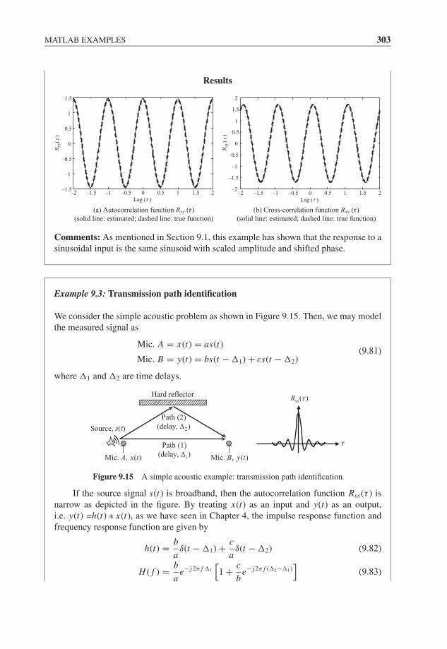
JWBK207-09 JWBK207-Shin January 30, 2008 15:55 Char Count= 0
MATLAB EXAMPLES 303
Results
Ryy
()
–2 –1.5 –1 –0.5 0 0.5 1 1.5 2–1.5
–1
–0.5
0
0.5
1
1.5
Lag (
(a) Autocorrelation function Ryy (τ)
(solid line: estimated; dashed line: true function)
(b) Cross-correlation function Rxy (τ)
(solid line: estimated; dashed line: true function)
)–2 –1.5 –1 –0.5 0 0.5 1 1.5 2
–2
–1.5
–1
–0.5
0
0.5
1
1.5
2
Lag ( )
Rxy
()
Comments: As mentioned in Section 9.1, this example has shown that the response to asinusoidal input is the same sinusoid with scaled amplitude and shifted phase.
Example 9.3: Transmission path identification
We consider the simple acoustic problem as shown in Figure 9.15. Then, we may modelthe measured signal as
Mic. A = x(t) = as(t)(9.81)
Mic. B = y(t) = bs(t − 1) + cs(t − 2)
where 1 and 2 are time delays.
Mic. , ( )B y t
Hard reflector
1
Path (1)
(delay, )
2
Path (2)
(delay, )
Mic. , ( )A x t
Source, s(t)
( )ssR
Figure 9.15 A simple acoustic example: transmission path identification
If the source signal s(t) is broadband, then the autocorrelation function Rss(τ ) isnarrow as depicted in the figure. By treating x(t) as an input and y(t) as an output,i.e. y(t) =h(t) ∗ x(t), as we have seen in Chapter 4, the impulse response function andfrequency response function are given by
h(t) = b
aδ(t − 1) + c
aδ(t − 2) (9.82)
H ( f ) = b
ae− j2π f 1
[1 + c
be− j2π f ( 2− 1)
](9.83)
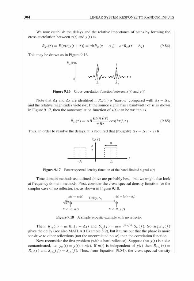
JWBK207-09 JWBK207-Shin January 30, 2008 15:55 Char Count= 0
304 LINEAR SYSTEM RESPONSE TO RANDOM INPUTS
We now establish the delays and the relative importance of paths by forming thecross-correlation between x(t) and y(t) as
Rxy(τ ) = E[x(t)y(t + τ )] = abRss(τ − 1) + acRss(τ − 2) (9.84)
This may be drawn as in Figure 9.16.
( )xyR
1 2
0
Figure 9.16 Cross-correlation function between x(t) and y(t)
Note that 1 and 2 are identified if Rss(τ ) is ‘narrow’ compared with 2 − 1,and the relative magnitudes yield b/c. If the source signal has a bandwidth of B as shownin Figure 9.17, then the autocorrelation function of s(t) can be written as
Rss(τ ) = ABsin(π Bτ )
π Bτcos(2π f0τ ) (9.85)
Thus, in order to resolve the delays, it is required that (roughly) 2 − 1 > 2/B.
0f
( )ssS f
0f
2
A
f
B
Figure 9.17 Power spectral density function of the band-limited signal s(t)
Time domain methods as outlined above are probably best – but we might also lookat frequency domain methods. First, consider the cross-spectral density function for thesimpler case of no reflector, i.e. as shown in Figure 9.18.
Mic. , ( )B ty
1Delay,
Mic. , ( )A tx
)( )(x ast t 1)y(t) bs(t
Figure 9.18 A simple acoustic example with no reflector
Then, Rxy(τ ) = abRss(τ − 1) and Sxy( f ) = abe− j2π f 1 Sss( f ). So arg Sxy( f )gives the delay (see also MATLAB Example 8.9), but it turns out that the phase is moresensitive to other reflections (not the uncorrelated noise) than the correlation function.
Now reconsider the first problem (with a hard reflector). Suppose that y(t) is noisecontaminated, i.e. ym(t) = y(t) + n(t). If n(t) is independent of y(t) then Rxym (τ ) =Rxy(τ ) and Sxym ( f ) = Sxy( f ). Thus, from Equation (9.84), the cross-spectral density
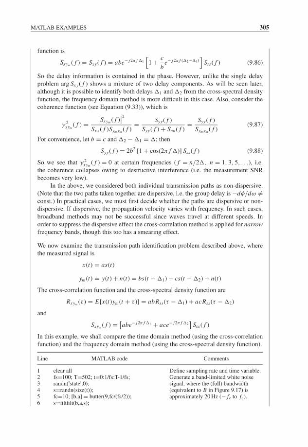
JWBK207-09 JWBK207-Shin January 30, 2008 15:55 Char Count= 0
MATLAB EXAMPLES 305
function is
Sxym ( f ) = Sxy( f ) = abe− j2π f 1
[1 + c
be− j2π f ( 2− 1)
]Sss( f ) (9.86)
So the delay information is contained in the phase. However, unlike the single delayproblem arg Sxy( f ) shows a mixture of two delay components. As will be seen later,although it is possible to identify both delays 1 and 2 from the cross-spectral densityfunction, the frequency domain method is more difficult in this case. Also, consider thecoherence function (see Equation (9.33)), which is
γ 2xym
( f ) =∣∣Sxym ( f )
∣∣2
Sxx ( f )Sym ym ( f )= Syy( f )
Syy( f ) + Snn( f )= Syy( f )
Sym ym ( f )(9.87)
For convenience, let b = c and 2 − 1 = ; then
Syy( f ) = 2b2 [1 + cos(2π f )] Sss( f ) (9.88)
So we see that γ 2xym
( f ) = 0 at certain frequencies ( f = n/2 , n = 1, 3, 5, . . .), i.e.the coherence collapses owing to destructive interference (i.e. the measurement SNRbecomes very low).
In the above, we considered both individual transmission paths as non-dispersive.(Note that the two paths taken together are dispersive, i.e. the group delay is −dφ/dω =const.) In practical cases, we must first decide whether the paths are dispersive or non-dispersive. If dispersive, the propagation velocity varies with frequency. In such cases,broadband methods may not be successful since waves travel at different speeds. Inorder to suppress the dispersive effect the cross-correlation method is applied for narrowfrequency bands, though this too has a smearing effect.
We now examine the transmission path identification problem described above, wherethe measured signal is
x(t) = as(t)
ym(t) = y(t) + n(t) = bs(t − 1) + cs(t − 2) + n(t)
The cross-correlation function and the cross-spectral density function are
Rxym (τ ) = E[x(t)ym(t + τ )] = abRss(τ − 1) + acRss(τ − 2)
and
Sxym ( f ) = [abe− j2π f 1 + ace− j2π f 2
]Sss( f )
In this example, we shall compare the time domain method (using the cross-correlationfunction) and the frequency domain method (using the cross-spectral density function).
Line MATLAB code Comments
123456
clear allfs=100; T=502; t=0:1/fs:T-1/fs;randn('state',0);s=randn(size(t));fc=10; [b,a] = butter(9,fc/(fs/2));s=filtfilt(b,a,s);
Define sampling rate and time variable.Generate a band-limited white noisesignal, where the (full) bandwidth(equivalent to B in Figure 9.17) isapproximately 20 Hz (− fc to fc).
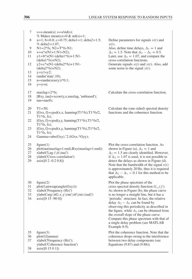
JWBK207-09 JWBK207-Shin January 30, 2008 15:55 Char Count= 0
306 LINEAR SYSTEM RESPONSE TO RANDOM INPUTS
7
8
91011
12
13141516
s=s-mean(s); s=s/std(s);% Makes mean(s)=0 & std(s)=1;a=1; b=0.8; c=0.75; delta1=1; delta2=1.5;% delta2=1.07;N1=2*fs; N2=T*fs-N1;x=a*s(N1+1:N1+N2);y1=b*s(N1-(delta1*fs)+1:N1-(delta1*fs)+N2);y2=c*s(N1-(delta2*fs)+1:N1-(delta2*fs)+N2);y=y1+y2;randn('state',10);n=randn(size(y))*0.1;y=y+n;
Define parameters for signals x(t) andy(t).Also, define time delays, 1 = 1 and 2 = 1.5. Note that 2 − 1 = 0.5.Later, use 2 = 1.07, and compare thecross-correlation functions.Generate signals x(t) and y(t). Also, addsome noise to the signal y(t).
171819
maxlag=2*fs;[Rxy, tau]=xcorr(y,x,maxlag, 'unbiased');tau=tau/fs;
Calculate the cross-correlation function.
2021
22
23
24
T1=50;[Gxx, f]=cpsd(x,x, hanning(T1*fs),T1*fs/2,T1*fs, fs);[Gyy, f]=cpsd(y,y, hanning(T1*fs),T1*fs/2,T1*fs, fs);[Gxy, f]=cpsd(x,y, hanning(T1*fs),T1*fs/2,T1*fs, fs);Gamma=abs(Gxy).ˆ2./(Gxx.*Gyy);
Calculate the (one-sided) spectral densityfunctions and the coherence function.
2526272829
figure(1)plot(tau(maxlag+1:end),Rxy(maxlag+1:end))xlabel('Lag (\it\tau)')ylabel('Cross-correlation')axis([0 2 -0.2 0.8])
Plot the cross-correlation function. Asshown in Figure (a), 1 = 1 and 2 = 1.5 are clearly identified. However,if 2 = 1.07 is used, it is not possible todetect the delays as shown in Figure (d).Note that the bandwidth of the signal s(t)is approximately 20 Hz, thus it is requiredthat 2 − 1 > 0.1 for this method to beapplicable.
3031323334
figure(2)plot(f,unwrap(angle(Gxy)))xlabel('Frequency (Hz)')ylabel('arg\itG x y\rm(\itf\rm) (rad)')axis([0 15 -90 0])
Plot the phase spectrum of thecross-spectral density function Gxy( f ).As shown in Figure (b), the phase curveis no longer a straight line, but it has a‘periodic’ structure. In fact, the relativedelay 2 − 1 can be found byobserving this periodicity as described inthe figure, while 1 can be obtained fromthe overall slope of the phase curve.Compare this phase spectrum with that ofa single delay problem (see MATLABExample 8.9).
353637
38
figure(3)plot(f,Gamma)xlabel('Frequency (Hz)');ylabel('Coherence function')axis([0 15 0 1])
Plot the coherence function. Note that thecoherence drops owing to the interferencebetween two delay components (seeEquations (9.87) and (9.88)).
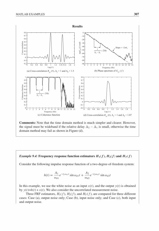
JWBK207-09 JWBK207-Shin January 30, 2008 15:55 Char Count= 0
MATLAB EXAMPLES 307
Results
0 0.2 0.4 0.6 0.8 1 1.2 1.4 1.6 1.8 21.5–0.2
–0.1
0
0.1
0.2
0.3
0.4
0.5
0.6
0.7
0.8
Lag ( )
Cro
ss-c
orr
elat
ion
0 1 2 3 4 5 6 7 8 9 10 11 12 13 14 15–90
–80
–70
–60
–50
–40
–30
–20
–10
0
Frequency (Hz)
arg
Gxy
(f)
(rad
)
1Slope 2
2 1
12 Hz
(a) Cross-correlation Rxy ( ), Δ1 = 1 and Δ2 = 1.5τ
(d) Cross-correlation Rxy (τ), Δ1 = 1 and Δ2 = 1.07
(b) Phase spectrum of Gxy ( f )
0 1 2 3 4 5 6 7 8 9 10 11 12 13 14 150
0.1
0.2
0.3
0.4
0.5
0.6
0.7
0.8
0.9
1
Frequency (Hz)
Coher
ence
funct
ion
2 1
12Hz
0 0.2 0.4 0.6 0.8 1 1.2 1.4 1.6 1.8 2–0.2
–0.1
0
0.1
0.2
0.3
0.4
0.5
0.6
0.7
0.8
Lag ( )
Cro
ss-c
orr
elat
ion
(c) Coherence function
Comments: Note that the time domain method is much simpler and clearer. However,the signal must be wideband if the relative delay 2 − 1 is small, otherwise the timedomain method may fail as shown in Figure (d).
Example 9.4: Frequency response function estimators H1( f ), H2( f ) and HT ( f )
Consider the following impulse response function of a two-degree-of-freedom system:
h(t) = A1
ωd1
e−ζ1ωn1t sin ωd1t + A2
ωd2
e−ζ2ωn2t sin ωd2t
In this example, we use the white noise as an input x(t), and the output y(t) is obtainedby y(t)=h(t) ∗ x(t). We also consider the uncorrelated measurement noise.
Three FRF estimators, H1( f ), H2( f ), and HT ( f ), are compared for three differentcases: Case (a), output noise only; Case (b), input noise only; and Case (c), both inputand output noise.
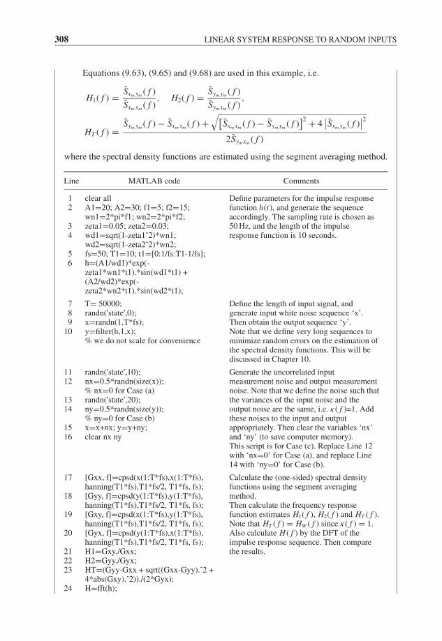
JWBK207-09 JWBK207-Shin January 30, 2008 15:55 Char Count= 0
308 LINEAR SYSTEM RESPONSE TO RANDOM INPUTS
Equations (9.63), (9.65) and (9.68) are used in this example, i.e.
H1( f ) = Sxm ym ( f )
Sxm xm ( f ), H2( f ) = Sym ym ( f )
Sym xm ( f ),
HT ( f ) =Sym ym ( f ) − Sxm xm ( f ) +
√[Sxm xm ( f ) − Sym ym ( f )
]2 + 4∣∣Sxm ym ( f )
∣∣2
2Sym xm ( f )
where the spectral density functions are estimated using the segment averaging method.
Line MATLAB code Comments
12
34
56
clear allA1=20; A2=30; f1=5; f2=15;wn1=2*pi*f1; wn2=2*pi*f2;zeta1=0.05; zeta2=0.03;wd1=sqrt(1-zeta1ˆ2)*wn1;wd2=sqrt(1-zeta2ˆ2)*wn2;fs=50; T1=10; t1=[0:1/fs:T1-1/fs];h=(A1/wd1)*exp(-zeta1*wn1*t1).*sin(wd1*t1) +(A2/wd2)*exp(-zeta2*wn2*t1).*sin(wd2*t1);
Define parameters for the impulse responsefunction h(t), and generate the sequenceaccordingly. The sampling rate is chosen as50 Hz, and the length of the impulseresponse function is 10 seconds.
789
10
T= 50000;randn('state',0);x=randn(1,T*fs);y=filter(h,1,x);% we do not scale for convenience
Define the length of input signal, andgenerate input white noise sequence ‘x’.Then obtain the output sequence ‘y’.Note that we define very long sequences tominimize random errors on the estimation ofthe spectral density functions. This will bediscussed in Chapter 10.
1112
1314
1516
randn('state',10);nx=0.5*randn(size(x));% nx=0 for Case (a)randn('state',20);ny=0.5*randn(size(y));% ny=0 for Case (b)x=x+nx; y=y+ny;clear nx ny
Generate the uncorrelated inputmeasurement noise and output measurementnoise. Note that we define the noise such thatthe variances of the input noise and theoutput noise are the same, i.e. κ( f )=1. Addthese noises to the input and outputappropriately. Then clear the variables ‘nx’and ‘ny’ (to save computer memory).This script is for Case (c). Replace Line 12with ‘nx=0’ for Case (a), and replace Line14 with ‘ny=0’ for Case (b).
17
18
19
20
212223
24
[Gxx, f]=cpsd(x(1:T*fs),x(1:T*fs),hanning(T1*fs),T1*fs/2, T1*fs, fs);[Gyy, f]=cpsd(y(1:T*fs),y(1:T*fs),hanning(T1*fs),T1*fs/2, T1*fs, fs);[Gxy, f]=cpsd(x(1:T*fs),y(1:T*fs),hanning(T1*fs),T1*fs/2, T1*fs, fs);[Gyx, f]=cpsd(y(1:T*fs),x(1:T*fs),hanning(T1*fs),T1*fs/2, T1*fs, fs);H1=Gxy./Gxx;H2=Gyy./Gyx;HT=(Gyy-Gxx + sqrt((Gxx-Gyy).ˆ2 +4*abs(Gxy).ˆ2))./(2*Gyx);H=fft(h);
Calculate the (one-sided) spectral densityfunctions using the segment averagingmethod.Then calculate the frequency responsefunction estimates H1( f ), H2( f ) and HT ( f ).Note that HT ( f ) = HW ( f ) since κ( f ) = 1.Also calculate H ( f ) by the DFT of theimpulse response sequence. Then comparethe results.
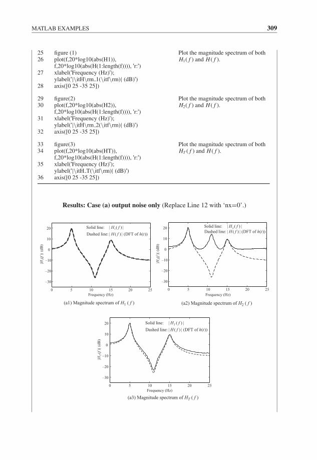
JWBK207-09 JWBK207-Shin January 30, 2008 15:55 Char Count= 0
MATLAB EXAMPLES 309
2526
27
28
figure (1)plot(f,20*log10(abs(H1)),f,20*log10(abs(H(1:length(f)))), 'r:')xlabel('Frequency (Hz)');ylabel('|\itH\rm 1(\itf\rm)| (dB)')axis([0 25 -35 25])
Plot the magnitude spectrum of bothH1( f ) and H ( f ).
2930
31
32
figure(2)plot(f,20*log10(abs(H2)),f,20*log10(abs(H(1:length(f)))), 'r:')xlabel('Frequency (Hz)');ylabel('|\itH\rm 2(\itf\rm)| (dB)')axis([0 25 -35 25])
Plot the magnitude spectrum of bothH2( f ) and H ( f ).
3334
35
36
figure(3)plot(f,20*log10(abs(HT)),f,20*log10(abs(H(1:length(f)))), 'r:')xlabel('Frequency (Hz)');ylabel('|\itH T(\itf\rm)| (dB)')axis([0 25 -35 25])
Plot the magnitude spectrum of bothHT ( f ) and H ( f ).
Results: Case (a) output noise only (Replace Line 12 with ‘nx=0’.)
1Solid line: | ( ) |
Dashed line: | ( ) | (DFT of ( ))
H f
H f h t
|H1(f
)|(d
B)
0 5 10 15 20 25
–30
–20
–10
0
10
20
Frequency (Hz)
|H2(f
)|(d
B)
0 5 10 15 20 25
–30
–20
–10
0
10
20
Frequency (Hz)
2Solid line: | ( ) |
Dashed line: | ( ) | (DFT of ( ))
H fH f h t
|HT
(f)|
(dB
)
Solid line: | ( ) |
Dashed line: | ( ) | (DFT of ( ))
TH f
H f h t
0 5 10 15 20 25
–30
–20
–10
0
10
20
Frequency (Hz)
(a1) Magnitude spectrum of H1 ( f ) (a2) Magnitude spectrum of H2 ( f )
(a3) Magnitude spectrum of HT ( f )

JWBK207-09 JWBK207-Shin January 30, 2008 15:55 Char Count= 0
310 LINEAR SYSTEM RESPONSE TO RANDOM INPUTS
Results: Case (b) input noise only (Replace Line 14 with ‘ny=0’.)|H
1(
f )|(
dB
)
1Solid line: | ( )|
Dashed line:| ( )| (DFT of ( ))
fH
fH h t
0 5 10 15 20 25
–30
–20
–10
0
10
20
Frequency (Hz)
|H2(
f )|(
dB
)
2Solid line: | ( )|
Dashed line:| ( )| (DFT of ( ))
fH
fH h t
0 5 10 15 20 25
–30
–20
–10
0
10
20
Frequency (Hz)
|HT
( f )
|(dB
)
Solid line: | ( )|
Dashed line:| ( )| (DFT of ( ))
T fH
fH h t
0 5 10 15 20 25
–30
–20
–10
0
10
20
Frequency (Hz)
(b1) Magnitude spectrum of H1 ( f ) (b2) Magnitude spectrum of H2 ( f )
(b3) Magnitude spectrum of HT ( f )
Results: Case (c) both input and output noise
|H1(
f)|(
dB
)
|HT
(f)
|(dB
)
|H2(
f)|(
dB
)
1Solid line: | ( ) |
Dashed line: | ( ) | (DFT of ( ))
H f
H f h t
0 5 10 15 20 25
–30
–20
–10
0
10
20
Frequency (Hz)
2Solid line: | ( ) |
Dashed line: | ( ) | (DFT of h( ))
H fH f t
0 5 10 15 20 25
–30
–20
–10
0
10
20
Frequency (Hz)
Solid line: | ( ) |
Dashed line: | ( ) | (DFT of ( ))
TH f
H f h t
0 5 10 15 20 25
–30
–20
–10
0
10
20
Frequency (Hz)
(c1) Magnitude spectrum of H1 ( f ) (c2) Magnitude spectrum of H2 ( f )
(c3) Magnitude spectrum of HT ( f )
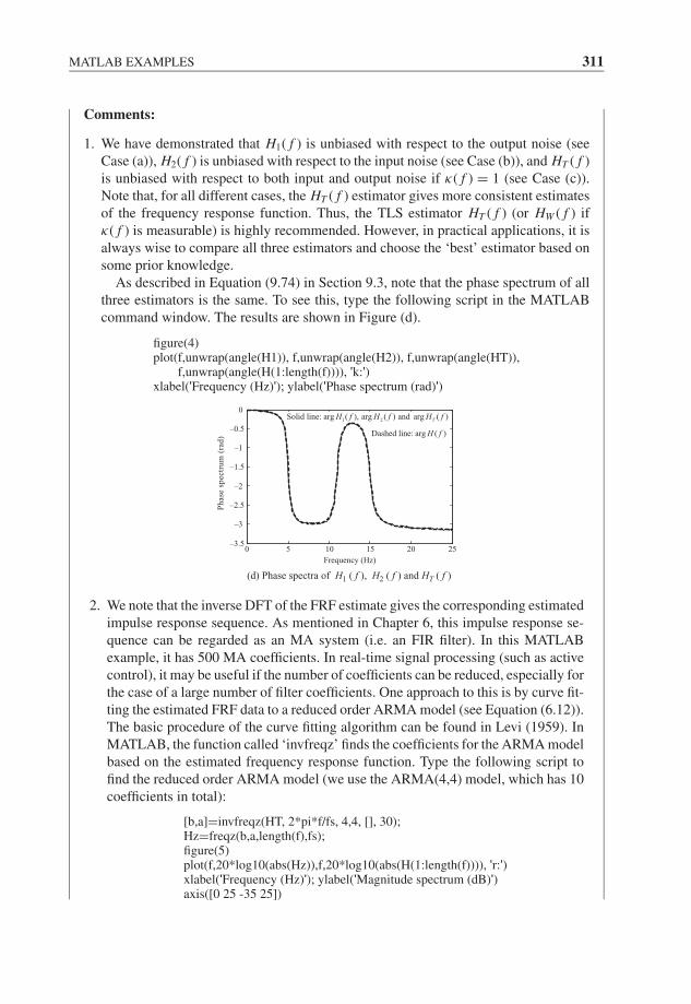
JWBK207-09 JWBK207-Shin January 30, 2008 15:55 Char Count= 0
MATLAB EXAMPLES 311
Comments:
1. We have demonstrated that H1( f ) is unbiased with respect to the output noise (seeCase (a)), H2( f ) is unbiased with respect to the input noise (see Case (b)), and HT ( f )is unbiased with respect to both input and output noise if κ( f ) = 1 (see Case (c)).Note that, for all different cases, the HT ( f ) estimator gives more consistent estimatesof the frequency response function. Thus, the TLS estimator HT ( f ) (or HW ( f ) ifκ( f ) is measurable) is highly recommended. However, in practical applications, it isalways wise to compare all three estimators and choose the ‘best’ estimator based onsome prior knowledge.
As described in Equation (9.74) in Section 9.3, note that the phase spectrum of allthree estimators is the same. To see this, type the following script in the MATLABcommand window. The results are shown in Figure (d).
figure(4)plot(f,unwrap(angle(H1)), f,unwrap(angle(H2)), f,unwrap(angle(HT)),
f,unwrap(angle(H(1:length(f)))), 'k:')xlabel('Frequency (Hz)'); ylabel('Phase spectrum (rad)')
0 5 10 15 20 25–3.5
–3
–2.5
–2
–1.5
–1
–0.5
0
Frequency (Hz)
Ph
ase
spec
tru
m (
rad
)
1 2Solid line: arg ( ), arg ( ) and arg ( )TH f H f H f
Dashed line: arg ( )H f
(d) Phase spectra of H1 ( f ), H2 ( f ) and HT ( f )
2. We note that the inverse DFT of the FRF estimate gives the corresponding estimatedimpulse response sequence. As mentioned in Chapter 6, this impulse response se-quence can be regarded as an MA system (i.e. an FIR filter). In this MATLABexample, it has 500 MA coefficients. In real-time signal processing (such as activecontrol), it may be useful if the number of coefficients can be reduced, especially forthe case of a large number of filter coefficients. One approach to this is by curve fit-ting the estimated FRF data to a reduced order ARMA model (see Equation (6.12)).The basic procedure of the curve fitting algorithm can be found in Levi (1959). InMATLAB, the function called ‘invfreqz’ finds the coefficients for the ARMA modelbased on the estimated frequency response function. Type the following script tofind the reduced order ARMA model (we use the ARMA(4,4) model, which has 10coefficients in total):
[b,a]=invfreqz(HT, 2*pi*f/fs, 4,4, [], 30);Hz=freqz(b,a,length(f),fs);figure(5)plot(f,20*log10(abs(Hz)),f,20*log10(abs(H(1:length(f)))), 'r:')xlabel('Frequency (Hz)'); ylabel('Magnitude spectrum (dB)')axis([0 25 -35 25])

JWBK207-09 JWBK207-Shin January 30, 2008 15:55 Char Count= 0
312 LINEAR SYSTEM RESPONSE TO RANDOM INPUTS
figure(6)plot(f,unwrap(angle(Hz)), f,unwrap(angle(H(1:length(f)))), 'r:')xlabel('Frequency (Hz)'); ylabel('Phase spectrum (rad)')
The first line of the MATLAB script finds the coefficients for the ARMA(4,4) modelbased on the estimated FRF (we use the results of HT ( f ) in this example), and the secondline evaluates the frequency response HZ ( f ) based on the coefficient vectors ‘a’ and ‘b’obtained from the first line. Then, plot both magnitude and phase spectra of HZ ( f ) andcompare with those of H ( f ). The results are as in Figures (e) and (f).
0 5 10 15 20 25
–30
–20
–10
0
10
20
Frequency (Hz)
Mag
nit
ude
spec
trum
(dB
)
Solid line: | ( ) |
Dashed line: | ( ) | (DFT of ( ))
ZH f
H f h t
0 5 10 15 20 25–3.5
–3
–2.5
–2
–1.5
–1
–0.5
0
Frequency (Hz)
Ph
ase
spec
tru
m (
rad
)
Solid line: arg ( )
Dashed line: arg ( )ZH f
H f
(e) Magnitude spectra of HZ ( f ) and H( f ) (f) Phase spectra of HZ( f ) and H( f )
Example 9.5: A practical example of system identification
We consider the same experimental setup used in MATLAB Example 6.7 (impact testingof a structure), except that we use a band-limited white noise for the input signal as shownin Figure (a). In this experiment, the frequency band of the signal is set at 5 to 90 Hz andthe sampling rate is chosen as fs = 256 Hz.
Physical system
Estimated (digital) system, H(z)
H(s)
Accelerometer
Input(voltage)
Output
A (PZT patch)
B
x(t)
y(t)
Data recorder (with ADC)
(a) Experimental set-up
(with
Signal conditioner
anti-aliasing filter B)
Noise
Noise
Band-limitedwhite noise
Power amplifier
Anti-aliasing filter A
Voltage
In this example, we will compare the results of three different FRF estimators, H1( f ),H2( f ) and HT ( f ), using the measured data stored in the file ‘beam experiment.mat’.1
1The data files can be downloaded from the Companion Website (www.wiley.com/go/shin hammond).
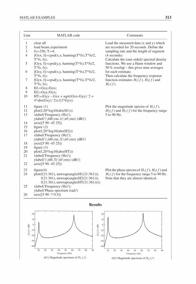
JWBK207-09 JWBK207-Shin January 30, 2008 15:55 Char Count= 0
MATLAB EXAMPLES 313
Line MATLAB code Comments
1234
5
6
7
89
10
clear allload beam experimentfs=256; T=4;[Gxx, f]=cpsd(x,x, hanning(T*fs),T*fs/2,T*fs, fs);[Gyy, f]=cpsd(y,y, hanning(T*fs),T*fs/2,T*fs, fs);[Gxy, f]=cpsd(x,y, hanning(T*fs),T*fs/2,T*fs, fs);[Gyx, f]=cpsd(y,x, hanning(T*fs),T*fs/2,T*fs, fs);H1=Gxy./Gxx;H2=Gyy./Gyx;HT=(Gyy – Gxx + sqrt((Gxx-Gyy).ˆ2 +4*abs(Gxy).ˆ2))./(2*Gyx);
Load the measured data (x and y) whichare recorded for 20 seconds. Define thesampling rate and the length of segment(4 seconds).Calculate the (one-sided) spectral densityfunctions. We use a Hann window and50 % overlap – this gives nine averagesfor each estimate.Then calculate the frequency responsefunction estimates H1( f ), H2( f ) andHT ( f ).
111213
14151617
18192021
22
figure (1)plot(f,20*log10(abs(H1)))xlabel('Frequency (Hz)');ylabel('|\itH\rm 1(\itf\rm)| (dB)')axis([5 90 -45 25])figure (2)plot(f,20*log10(abs(H2)))xlabel('Frequency (Hz)');ylabel('|\itH\rm 2(\itf\rm)| (dB)')axis([5 90 -45 25])figure (3)plot(f,20*log10(abs(HT)))xlabel('Frequency (Hz)');ylabel('|\itH T(\itf\rm)| (dB)')axis([5 90 -45 25])
Plot the magnitude spectra of H1( f ),H2( f ) and HT ( f ) for the frequency range5 to 90 Hz.
2324
25
26
figure(4)plot(f(21:361), unwrap(angle(H1(21:361))),
f(21:361), unwrap(angle(H2(21:361))),f(21:361), unwrap(angle(HT(21:361))));
xlabel('Frequency (Hz)');ylabel('Phase spectrum (rad)')axis([5 90 -7 0.5])
Plot the phase spectra of H1( f ), H2( f ) andHT ( f ) for the frequency range 5 to 90 Hz.Note that they are almost identical.
Results
|H1(f
)|(d
B)
10 20 30 40 50 60 70 80 90
–40
–30
–20
–10
0
10
20
Frequency (Hz)
|H2(
f)|
(dB
)
10 20 30 40 50 60 70 80 90
–40
–30
–20
–10
0
10
20
Frequency (Hz)
(b1) Magnitude spectrum of H1 ( f ) (b2) Magnitude spectrum of H2 ( f )

JWBK207-09 JWBK207-Shin January 30, 2008 15:55 Char Count= 0
314 LINEAR SYSTEM RESPONSE TO RANDOM INPUTS
|HT
(f)
|(d
B)
10 20 30 40 50 60 70 80 90
–40
–30
–20
–10
0
10
20
Frequency (Hz)
10 20 30 40 50 60 70 80 90–7
–6
–5
–4
–3
–2
–1
0
Frequency (Hz)
Phas
e sp
ectr
um
(ra
d) 1 2arg ( ) arg ( ) arg ( )TH f H f H f
(b3) Magnitude spectrum of HT ( f ) (b4) Phase spectra of H1 ( f ), H2 ( f ) and HT ( f )
Comments:
1. As shown in Figure (b4), the phase spectra of H1( f ), H2( f ) and HT ( f ) are the same.However, the results of magnitude spectra show that H1( f ) considerably underes-timates at resonances compared with other estimates H2( f ) and HT ( f ). Figure (c)shows the differences in detail.
(c) Magnitude spectra of H1( f ), H2( f ) and HT( f )
10
0
10
20
( )
2 ( )H f
( )TH f
10 20 30 40 50 60 70 80 90
–40
–30
–20
–
Frequency (Hz)
Mag
nit
ude
spec
tru
m (
dB
)
1( )H f
( )
( )
Also, plot the coherence function by typing the following script. The result is shownin Figure (d).
figure(5)Gamma=abs(Gxy).ˆ2./(Gxx.*Gyy);plot(f, Gamma); axis([5 90 0 1.1])xlabel('Frequency (Hz)'); ylabel('Coherence function')
Note that the value of the coherence function drops at resonances due to the biaserror, which will be discussed in Chapter 10 (see also Comments 1 in MATLABExample 9.1).
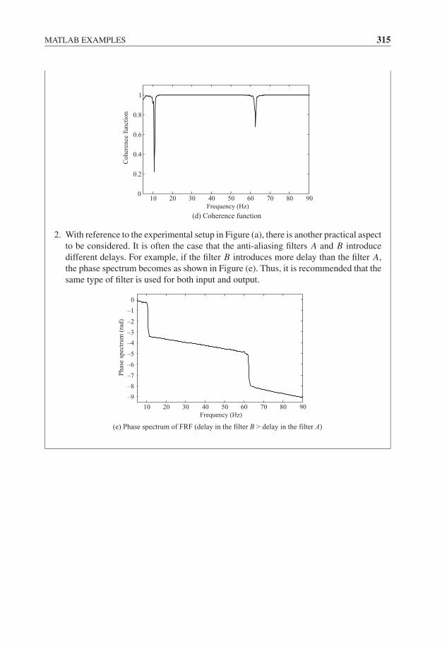
JWBK207-09 JWBK207-Shin January 30, 2008 15:55 Char Count= 0
MATLAB EXAMPLES 315
10 20 30 40 50 60 70 80 900
0.2
0.4
0.6
0.8
1
Frequency (Hz)
Coher
ence
funct
ion
(d) Coherence function
2. With reference to the experimental setup in Figure (a), there is another practical aspectto be considered. It is often the case that the anti-aliasing filters A and B introducedifferent delays. For example, if the filter B introduces more delay than the filter A,the phase spectrum becomes as shown in Figure (e). Thus, it is recommended that thesame type of filter is used for both input and output.
10 20 30 40 50 60 70 80 90
–9
–8
–7
–6
–5
–4
–3
–2
–1
0
Frequency (Hz)
(e) Phase spectrum of FRF (delay in the filter B > delay in the filter A)
Ph
ase
spec
tru
m (
rad
)

JWBK207-09 JWBK207-Shin January 30, 2008 15:55 Char Count= 0
316
JWBK207-10 JWBK207-Shin January 18, 2008 8:20 Char Count= 0
10Estimation Methods and StatisticalConsiderations
Introduction
So far, we have discussed random processes in terms of ideal quantities: probabilitydensity functions, correlation functions and spectral density functions. The results inChapter 9 used these theoretical concepts, and the MATLAB examples used estimationmethods that anticipated what is presented in this chapter. In this chapter, we introducestatistical estimation methods for random signals based on a single realization (record) ofthe process, and show how the theoretical quantities may be estimated and the accuracyof these estimates.
While omitting many mathematical justifications, the details of results quoted inthis chapter may be found in many of the references, especially in Jenkins and Watts(1968) and Bendat and Piersol (2000). Readers who wish to know the details of statisticalproperties of random processes should refer to these two excellent texts.
10.1 ESTIMATOR ERRORS AND ACCURACY
Suppose we only have a single time record x(t) with a length of T , taken from a stochasticprocess. If we want to know the mean value μx of the process, then a logical estimate(denoted by x) of μx is
x = 1
T
T∫0
x(t)dt (10.1)
Fundamentals of Signal Processing for Sound and Vibration EngineersK. Shin and J. K. Hammond. C© 2008 John Wiley & Sons, Ltd
317
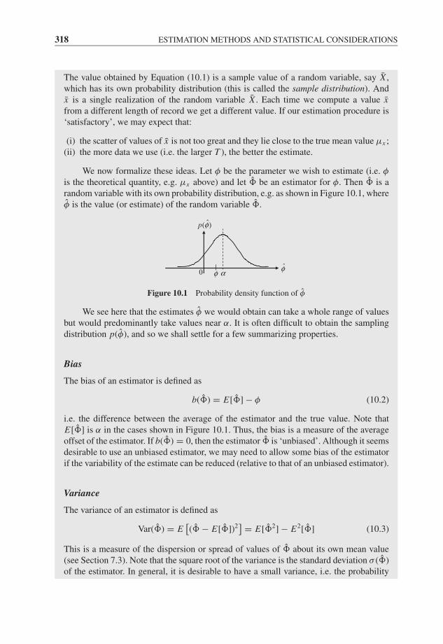
JWBK207-10 JWBK207-Shin January 18, 2008 8:20 Char Count= 0
318 ESTIMATION METHODS AND STATISTICAL CONSIDERATIONS
The value obtained by Equation (10.1) is a sample value of a random variable, say X ,which has its own probability distribution (this is called the sample distribution). Andx is a single realization of the random variable X . Each time we compute a value xfrom a different length of record we get a different value. If our estimation procedure is‘satisfactory’, we may expect that:
(i) the scatter of values of x is not too great and they lie close to the true mean value μx ;(ii) the more data we use (i.e. the larger T ), the better the estimate.
We now formalize these ideas. Let φ be the parameter we wish to estimate (i.e. φ
is the theoretical quantity, e.g. μx above) and let � be an estimator for φ. Then � is arandom variable with its own probability distribution, e.g. as shown in Figure 10.1, whereφ is the value (or estimate) of the random variable �.
ˆ( )p φ
φφ α0
Figure 10.1 Probability density function of φ
We see here that the estimates φ we would obtain can take a whole range of valuesbut would predominantly take values near α. It is often difficult to obtain the samplingdistribution p(φ), and so we shall settle for a few summarizing properties.
Bias
The bias of an estimator is defined as
b(�) = E[�] − φ (10.2)
i.e. the difference between the average of the estimator and the true value. Note thatE[�] is α in the cases shown in Figure 10.1. Thus, the bias is a measure of the averageoffset of the estimator. If b(�) = 0, then the estimator � is ‘unbiased’. Although it seemsdesirable to use an unbiased estimator, we may need to allow some bias of the estimatorif the variability of the estimate can be reduced (relative to that of an unbiased estimator).
Variance
The variance of an estimator is defined as
Var(�) = E[(� − E[�])2
] = E[�2] − E2[�] (10.3)
This is a measure of the dispersion or spread of values of � about its own mean value(see Section 7.3). Note that the square root of the variance is the standard deviation σ (�)of the estimator. In general, it is desirable to have a small variance, i.e. the probability
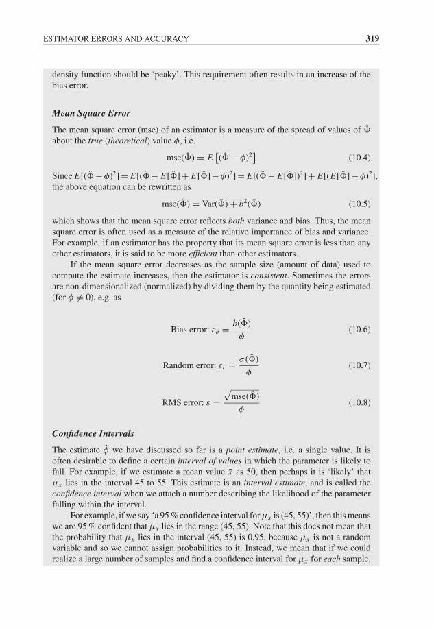
JWBK207-10 JWBK207-Shin January 18, 2008 8:20 Char Count= 0
ESTIMATOR ERRORS AND ACCURACY 319
density function should be ‘peaky’. This requirement often results in an increase of thebias error.
Mean Square Error
The mean square error (mse) of an estimator is a measure of the spread of values of �
about the true (theoretical) value φ, i.e.
mse(�) = E[(� − φ)2
](10.4)
Since E[(� − φ)2] = E[(� − E[�] + E[�] − φ)2] = E[(� − E[�])2] + E[(E[�] − φ)2],the above equation can be rewritten as
mse(�) = Var(�) + b2(�) (10.5)
which shows that the mean square error reflects both variance and bias. Thus, the meansquare error is often used as a measure of the relative importance of bias and variance.For example, if an estimator has the property that its mean square error is less than anyother estimators, it is said to be more efficient than other estimators.
If the mean square error decreases as the sample size (amount of data) used tocompute the estimate increases, then the estimator is consistent. Sometimes the errorsare non-dimensionalized (normalized) by dividing them by the quantity being estimated(for φ �= 0), e.g. as
Bias error: εb = b(�)
φ(10.6)
Random error: εr = σ (�)
φ(10.7)
RMS error: ε =√
mse(�)
φ(10.8)
Confidence Intervals
The estimate φ we have discussed so far is a point estimate, i.e. a single value. It isoften desirable to define a certain interval of values in which the parameter is likely tofall. For example, if we estimate a mean value x as 50, then perhaps it is ‘likely’ thatμx lies in the interval 45 to 55. This estimate is an interval estimate, and is called theconfidence interval when we attach a number describing the likelihood of the parameterfalling within the interval.
For example, if we say ‘a 95 % confidence interval for μx is (45, 55)’, then this meanswe are 95 % confident that μx lies in the range (45, 55). Note that this does not mean thatthe probability that μx lies in the interval (45, 55) is 0.95, because μx is not a randomvariable and so we cannot assign probabilities to it. Instead, we mean that if we couldrealize a large number of samples and find a confidence interval for μx for each sample,
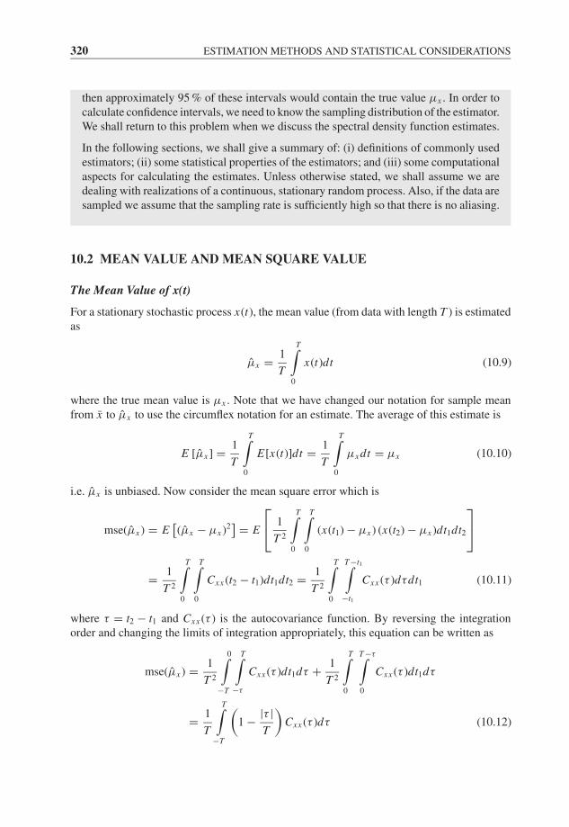
JWBK207-10 JWBK207-Shin January 18, 2008 8:20 Char Count= 0
320 ESTIMATION METHODS AND STATISTICAL CONSIDERATIONS
then approximately 95 % of these intervals would contain the true value μx . In order tocalculate confidence intervals, we need to know the sampling distribution of the estimator.We shall return to this problem when we discuss the spectral density function estimates.
In the following sections, we shall give a summary of: (i) definitions of commonly usedestimators; (ii) some statistical properties of the estimators; and (iii) some computationalaspects for calculating the estimates. Unless otherwise stated, we shall assume we aredealing with realizations of a continuous, stationary random process. Also, if the data aresampled we assume that the sampling rate is sufficiently high so that there is no aliasing.
10.2 MEAN VALUE AND MEAN SQUARE VALUE
The Mean Value of x(t)
For a stationary stochastic process x(t), the mean value (from data with length T ) is estimatedas
μx = 1
T
T∫0
x(t)dt (10.9)
where the true mean value is μx . Note that we have changed our notation for sample meanfrom x to μx to use the circumflex notation for an estimate. The average of this estimate is
E [μx ] = 1
T
T∫0
E[x(t)]dt = 1
T
T∫0
μx dt = μx (10.10)
i.e. μx is unbiased. Now consider the mean square error which is
mse(μx ) = E[(μx − μx )2
] = E
⎡⎣ 1
T 2
T∫0
T∫0
(x(t1) − μx ) (x(t2) − μx )dt1dt2
⎤⎦= 1
T 2
T∫0
T∫0
Cxx (t2 − t1)dt1dt2 = 1
T 2
T∫0
T −t1∫−t1
Cxx (τ )dτdt1 (10.11)
where τ = t2 − t1 and Cxx (τ ) is the autocovariance function. By reversing the integrationorder and changing the limits of integration appropriately, this equation can be written as
mse(μx ) = 1
T 2
0∫−T
T∫−τ
Cxx (τ )dt1dτ + 1
T 2
T∫0
T −τ∫0
Cxx (τ )dt1dτ
= 1
T
T∫−T
(1 − |τ |
T
)Cxx (τ )dτ (10.12)
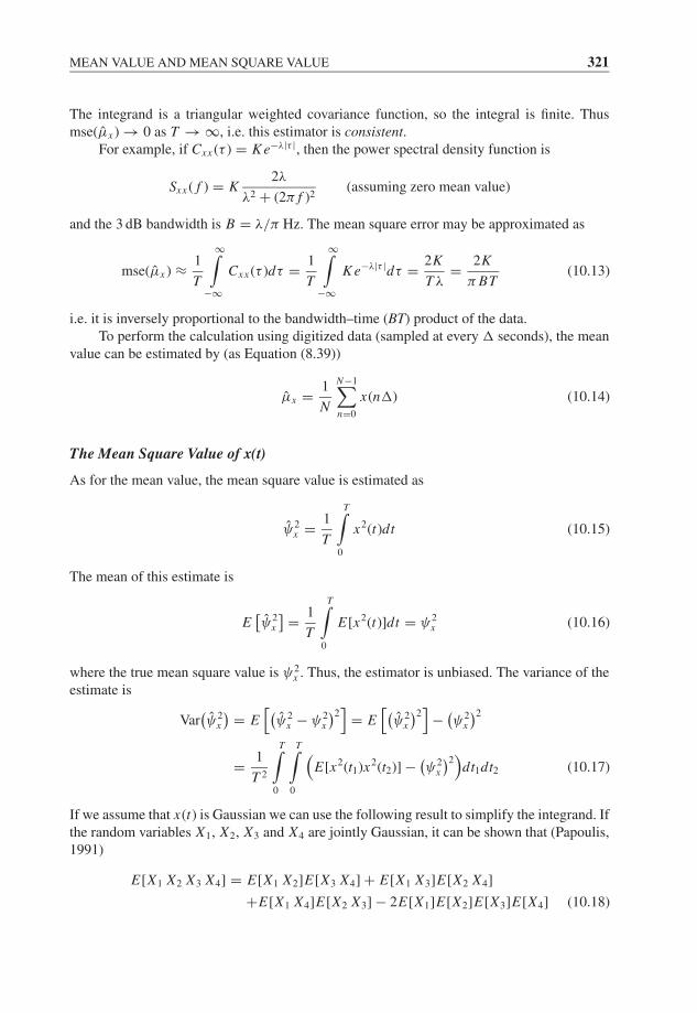
JWBK207-10 JWBK207-Shin January 18, 2008 8:20 Char Count= 0
MEAN VALUE AND MEAN SQUARE VALUE 321
The integrand is a triangular weighted covariance function, so the integral is finite. Thusmse(μx ) → 0 as T → ∞, i.e. this estimator is consistent.
For example, if Cxx (τ ) = K e−λ|τ |, then the power spectral density function is
Sxx ( f ) = K2λ
λ2 + (2π f )2(assuming zero mean value)
and the 3 dB bandwidth is B = λ/π Hz. The mean square error may be approximated as
mse(μx ) ≈ 1
T
∞∫−∞
Cxx (τ )dτ = 1
T
∞∫−∞
K e−λ|τ |dτ = 2K
T λ= 2K
π BT(10.13)
i.e. it is inversely proportional to the bandwidth–time (BT) product of the data.To perform the calculation using digitized data (sampled at every seconds), the mean
value can be estimated by (as Equation (8.39))
μx = 1
N
N−1∑n=0
x(n) (10.14)
The Mean Square Value of x(t)
As for the mean value, the mean square value is estimated as
ψ2x = 1
T
T∫0
x2(t)dt (10.15)
The mean of this estimate is
E[ψ2
x
] = 1
T
T∫0
E[x2(t)]dt = ψ2x (10.16)
where the true mean square value is ψ2x . Thus, the estimator is unbiased. The variance of the
estimate is
Var(ψ2
x
) = E[(
ψ2x − ψ2
x
)2]
= E[(
ψ2x
)2]
− (ψ2
x
)2
= 1
T 2
T∫0
T∫0
(E[x2(t1)x2(t2)] − (
ψ2x
)2)
dt1dt2 (10.17)
If we assume that x(t) is Gaussian we can use the following result to simplify the integrand. Ifthe random variables X1, X2, X3 and X4 are jointly Gaussian, it can be shown that (Papoulis,1991)
E[X1 X2 X3 X4] = E[X1 X2]E[X3 X4] + E[X1 X3]E[X2 X4]
+E[X1 X4]E[X2 X3] − 2E[X1]E[X2]E[X3]E[X4] (10.18)
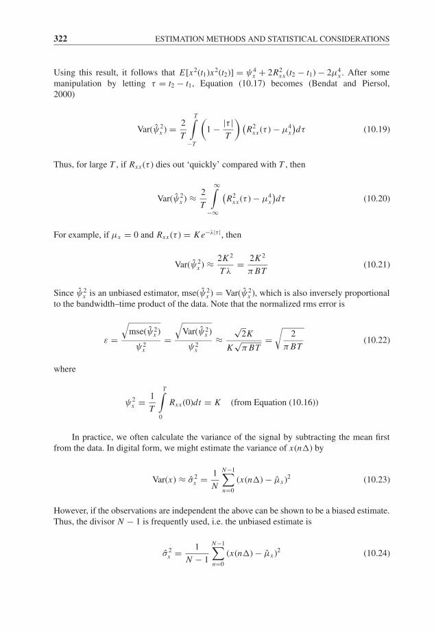
JWBK207-10 JWBK207-Shin January 18, 2008 8:20 Char Count= 0
322 ESTIMATION METHODS AND STATISTICAL CONSIDERATIONS
Using this result, it follows that E[x2(t1)x2(t2)] = ψ4x + 2R2
xx (t2 − t1) − 2μ4x . After some
manipulation by letting τ = t2 − t1, Equation (10.17) becomes (Bendat and Piersol,2000)
Var(ψ2x ) = 2
T
T∫−T
(1 − |τ |
T
) (R2
xx (τ ) − μ4x
)dτ (10.19)
Thus, for large T , if Rxx (τ ) dies out ‘quickly’ compared with T , then
Var(ψ2x ) ≈ 2
T
∞∫−∞
(R2
xx (τ ) − μ4x
)dτ (10.20)
For example, if μx = 0 and Rxx (τ ) = K e−λ|τ |, then
Var(ψ2x ) ≈ 2K 2
T λ= 2K 2
π BT(10.21)
Since ψ2x is an unbiased estimator, mse(ψ2
x ) = Var(ψ2x ), which is also inversely proportional
to the bandwidth–time product of the data. Note that the normalized rms error is
ε =√
mse(ψ2x )
ψ2x
=√
Var(ψ2x )
ψ2x
≈√
2K
K√
π BT=
√2
π BT(10.22)
where
ψ2x = 1
T
T∫0
Rxx (0)dt = K (from Equation (10.16))
In practice, we often calculate the variance of the signal by subtracting the mean firstfrom the data. In digital form, we might estimate the variance of x(n) by
Var(x) ≈ σ 2x = 1
N
N−1∑n=0
(x(n) − μx )2 (10.23)
However, if the observations are independent the above can be shown to be a biased estimate.Thus, the divisor N − 1 is frequently used, i.e. the unbiased estimate is
σ 2x = 1
N − 1
N−1∑n=0
(x(n) − μx )2 (10.24)
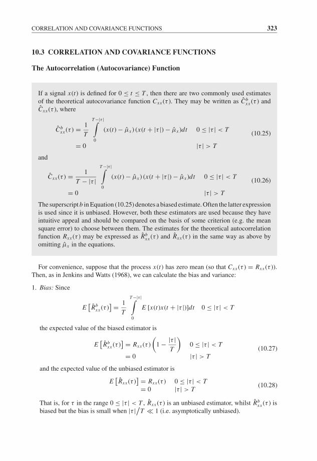
JWBK207-10 JWBK207-Shin January 18, 2008 8:20 Char Count= 0
CORRELATION AND COVARIANCE FUNCTIONS 323
10.3 CORRELATION AND COVARIANCE FUNCTIONS
The Autocorrelation (Autocovariance) Function
If a signal x(t) is defined for 0 ≤ t ≤ T , then there are two commonly used estimatesof the theoretical autocovariance function Cxx (τ ). They may be written as Cb
xx (τ ) andCxx (τ ), where
Cbxx (τ ) = 1
T
T −|τ |∫0
(x(t) − μx ) (x(t + |τ |) − μx )dt 0 ≤ |τ | < T
= 0 |τ | > T
(10.25)
and
Cxx (τ ) = 1
T − |τ |
T −|τ |∫0
(x(t) − μx ) (x(t + |τ |) − μx )dt 0 ≤ |τ | < T
= 0 |τ | > T
(10.26)
The superscript b in Equation (10.25) denotes a biased estimate. Often the latter expressionis used since it is unbiased. However, both these estimators are used because they haveintuitive appeal and should be compared on the basis of some criterion (e.g. the meansquare error) to choose between them. The estimates for the theoretical autocorrelationfunction Rxx (τ ) may be expressed as Rb
xx (τ ) and Rxx (τ ) in the same way as above byomitting μx in the equations.
For convenience, suppose that the process x(t) has zero mean (so that Cxx (τ ) = Rxx (τ )).Then, as in Jenkins and Watts (1968), we can calculate the bias and variance:
1. Bias: Since
E[Rb
xx (τ )] = 1
T
T −|τ |∫0
E [x(t)x(t + |τ |)]dt 0 ≤ |τ | < T
the expected value of the biased estimator is
E[Rb
xx (τ )] = Rxx (τ )
(1 − |τ |
T
)0 ≤ |τ | < T
= 0 |τ | > T(10.27)
and the expected value of the unbiased estimator is
E[Rxx (τ )
] = Rxx (τ ) 0 ≤ |τ | < T= 0 |τ | > T
(10.28)
That is, for τ in the range 0 ≤ |τ | < T , Rxx (τ ) is an unbiased estimator, whilst Rbxx (τ ) is
biased but the bias is small when |τ |/T 1 (i.e. asymptotically unbiased).
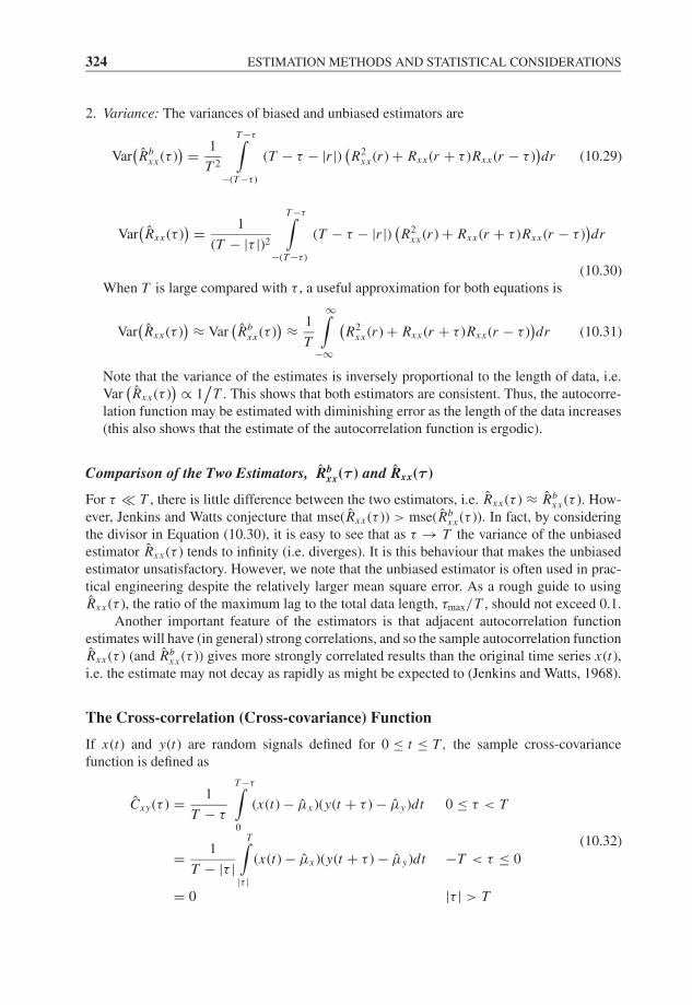
JWBK207-10 JWBK207-Shin January 18, 2008 8:20 Char Count= 0
324 ESTIMATION METHODS AND STATISTICAL CONSIDERATIONS
2. Variance: The variances of biased and unbiased estimators are
Var(Rb
xx (τ )) = 1
T 2
T −τ∫−(T −τ )
(T − τ − |r |) (R2
xx (r ) + Rxx (r + τ )Rxx (r − τ ))dr (10.29)
Var(Rxx (τ )
) = 1
(T − |τ |)2
T −τ∫−(T −τ )
(T − τ − |r |) (R2
xx (r ) + Rxx (r + τ )Rxx (r − τ ))dr
(10.30)When T is large compared with τ , a useful approximation for both equations is
Var(Rxx (τ )
) ≈ Var(Rb
xx (τ )) ≈ 1
T
∞∫−∞
(R2
xx (r ) + Rxx (r + τ )Rxx (r − τ ))dr (10.31)
Note that the variance of the estimates is inversely proportional to the length of data, i.e.Var
(Rxx (τ )
) ∝ 1/
T . This shows that both estimators are consistent. Thus, the autocorre-lation function may be estimated with diminishing error as the length of the data increases(this also shows that the estimate of the autocorrelation function is ergodic).
Comparison of the Two Estimators, Rbxx(τ ) and Rxx(τ )
For τ T , there is little difference between the two estimators, i.e. Rxx (τ ) ≈ Rbxx (τ ). How-
ever, Jenkins and Watts conjecture that mse(Rxx (τ )) > mse(Rbxx (τ )). In fact, by considering
the divisor in Equation (10.30), it is easy to see that as τ → T the variance of the unbiasedestimator Rxx (τ ) tends to infinity (i.e. diverges). It is this behaviour that makes the unbiasedestimator unsatisfactory. However, we note that the unbiased estimator is often used in prac-tical engineering despite the relatively larger mean square error. As a rough guide to usingRxx (τ ), the ratio of the maximum lag to the total data length, τmax/T , should not exceed 0.1.
Another important feature of the estimators is that adjacent autocorrelation functionestimates will have (in general) strong correlations, and so the sample autocorrelation functionRxx (τ ) (and Rb
xx (τ )) gives more strongly correlated results than the original time series x(t),i.e. the estimate may not decay as rapidly as might be expected to (Jenkins and Watts, 1968).
The Cross-correlation (Cross-covariance) Function
If x(t) and y(t) are random signals defined for 0 ≤ t ≤ T, the sample cross-covariancefunction is defined as
Cxy(τ ) = 1
T − τ
T −τ∫0
(x(t) − μx )(y(t + τ ) − μy)dt 0 ≤ τ < T
= 1
T − |τ |
T∫|τ |
(x(t) − μx )(y(t + τ ) − μy)dt −T < τ ≤ 0
= 0 |τ | > T
(10.32)
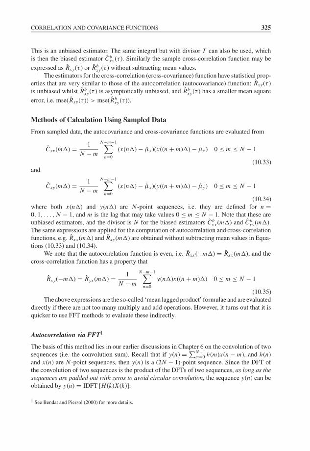
JWBK207-10 JWBK207-Shin January 18, 2008 8:20 Char Count= 0
CORRELATION AND COVARIANCE FUNCTIONS 325
This is an unbiased estimator. The same integral but with divisor T can also be used, whichis then the biased estimator Cb
xy(τ ). Similarly the sample cross-correlation function may be
expressed as Rxy(τ ) or Rbxy(τ ) without subtracting mean values.
The estimators for the cross-correlation (cross-covariance) function have statistical prop-erties that are very similar to those of the autocorrelation (autocovariance) function: Rxy(τ )is unbiased whilst Rb
xy(τ ) is asymptotically unbiased, and Rbxy(τ ) has a smaller mean square
error, i.e. mse(Rxy(τ )) > mse(Rbxy(τ )).
Methods of Calculation Using Sampled Data
From sampled data, the autocovariance and cross-covariance functions are evaluated from
Cxx (m) = 1
N − m
N−m−1∑n=0
(x(n) − μx )(x((n + m)) − μx ) 0 ≤ m ≤ N − 1
(10.33)and
Cxy(m) = 1
N − m
N−m−1∑n=0
(x(n) − μx )(y((n + m)) − μy) 0 ≤ m ≤ N − 1
(10.34)where both x(n) and y(n) are N -point sequences, i.e. they are defined for n =0, 1, . . . , N − 1, and m is the lag that may take values 0 ≤ m ≤ N − 1. Note that these areunbiased estimators, and the divisor is N for the biased estimators Cb
xx (m) and Cbxy(m).
The same expressions are applied for the computation of autocorrelation and cross-correlationfunctions, e.g. Rxx (m) and Rxy(m) are obtained without subtracting mean values in Equa-tions (10.33) and (10.34).
We note that the autocorrelation function is even, i.e. Rxx (−m) = Rxx (m), and thecross-correlation function has a property that
Rxy(−m) = Ryx (m) = 1
N − m
N−m−1∑n=0
y(n)x((n + m)) 0 ≤ m ≤ N − 1
(10.35)The above expressions are the so-called ‘mean lagged product’ formulae and are evaluated
directly if there are not too many multiply and add operations. However, it turns out that it isquicker to use FFT methods to evaluate these indirectly.
Autocorrelation via FFT1
The basis of this method lies in our earlier discussions in Chapter 6 on the convolution of twosequences (i.e. the convolution sum). Recall that if y(n) = ∑N−1
m=0 h(m)x(n − m), and h(n)and x(n) are N -point sequences, then y(n) is a (2N − 1)-point sequence. Since the DFT ofthe convolution of two sequences is the product of the DFTs of two sequences, as long as thesequences are padded out with zeros to avoid circular convolution, the sequence y(n) can beobtained by y(n) = IDFT [H (k)X (k)].
1 See Bendat and Piersol (2000) for more details.
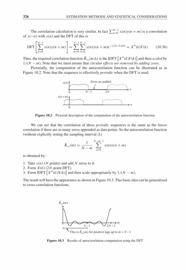
JWBK207-10 JWBK207-Shin January 18, 2008 8:20 Char Count= 0
326 ESTIMATION METHODS AND STATISTICAL CONSIDERATIONS
The correlation calculation is very similar. In fact∑N−1
n=0 x(n)y(n + m) is a convolutionof x(−n) with y(n) and the DFT of this is
DFT
[N−1∑n=0
x(n)y(n + m)
]=
N−1∑m=0
N−1∑n=0
x(n)y(n + m)e− j(2π/N )mk = X*(k)Y (k) (10.36)
Thus, the required correlation function Rxy(m) is the IDFT[X*(k)Y (k)
]and then scaled by
1/(N − m). Note that we must ensure that circular effects are removed by adding zeros.Pictorially, the computation of the autocorrelation function can be illustrated as in
Figure 10.2. Note that the sequence is effectively periodic when the DFT is used.
n
x(n) Zeros are padded
n
0
0
x(n m)+1N − 2N
Figure 10.2 Pictorial description of the computation of the autocorrelation function
We can see that the correlation of these periodic sequences is the same as the linearcorrelation if there are as many zeros appended as data points. So the autocorrelation function(without explicitly noting the sampling interval )
Rxx (m) = 1
N − m
N−m−1∑n=0
x(n)x(n + m)
is obtained by:
1. Take x(n) (N points) and add N zeros to it.2. Form X (k) (2N -point DFT).3. Form IDFT
[X*(k)X (k)
]and then scale appropriately by 1/(N − m).
The result will have the appearance as shown in Figure 10.3. This basic idea can be generalizedto cross-correlation functions.
ˆ ( )xxR m
1N − 2 1N −
ˆThis is ) for positive lags up to ( 1xxR m Nm −=
m
Figure 10.3 Results of autocorrelation computation using the DFT

JWBK207-10 JWBK207-Shin January 18, 2008 8:20 Char Count= 0
POWER SPECTRAL DENSITY FUNCTION 327
10.4 POWER SPECTRAL DENSITY FUNCTION
There are two main approaches to estimating the power spectral density function, namelyparametric (more recent) and non-parametric (traditional), as shown in Figure 10.4.
Estimation methods
Non-parametric Parametric(ARMA, maximum entropy, etc.)
Filter bank method(analogue method)
Indirect method(Fourier transform of
autocorrelation function)
Direct methods(e.g. segment averaging)
Figure 10.4 Classification of the estimation methods for the power spectral density function
Estimation methods for the power spectral density function considered here willrelate to the ‘traditional’ methods rather than ‘parametric’ methods. We shall outlinethree methods for the estimation of the power spectral density function:� Method (1): ‘Analogue’ method (filter bank method)� Method (2): Fourier transform of the autocorrelation function (indirect method)� Method (3): Direct methods.
Note that Method (3) is the most widely used since with the advent of the FFT it is thequickest.
Method (1): ‘Analogue’ Method (Filter Bank Method)
The word ‘analogue’ is in quotes because this method can also be implemented digitally, butit is convenient to refer to continuous signals. The basic scheme is indicated in Figure 10.5.
The basis of this method is that the variance of the signal is the area under the powerspectral density function curve (assuming zero mean value), i.e.
Var (x(t)) = σ 2x =
∞∫0
Gxx ( f )d f (10.37)
where Gxx ( f ) is regarded as a measure of the distribution of the power of the process overfrequency. So if we wish to know the power in the signal over some frequency band fc ± B/2,
x(t) Tunable narrow
band-pass filter
Centre frequency, fBandwidth, B
c
cx(t, f , B) Squarer,
integrator and averager
)( fxx cG
Figure 10.5 Concept of the filter bank method
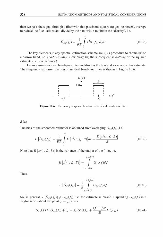
JWBK207-10 JWBK207-Shin January 18, 2008 8:20 Char Count= 0
328 ESTIMATION METHODS AND STATISTICAL CONSIDERATIONS
then we pass the signal through a filter with that passband, square (to get the power), averageto reduce the fluctuations and divide by the bandwidth to obtain the ‘density’, i.e.
Gxx ( fc) = 1
BT
T∫0
x2(t, fc, B)dt (10.38)
The key elements in any spectral estimation scheme are: (i) a procedure to ‘home in’ ona narrow band, i.e. good resolution (low bias); (ii) the subsequent smoothing of the squaredestimate (i.e. low variance).
Let us assume an ideal band-pass filter and discuss the bias and variance of this estimate.The frequency response function of an ideal band-pass filter is shown in Figure 10.6.
cfcf−
)(H f
f
1.0
B
Figure 10.6 Frequency response function of an ideal band-pass filter
Bias
The bias of the smoothed estimator is obtained from averaging Gxx ( fc), i.e.
E[Gxx ( fc)
] = 1
BT
T∫0
E[x2(t, fc, B)
]dt = E
[x2(t, fc, B)
]B
(10.39)
Note that E[x2(t, fc, B)
]is the variance of the output of the filter, i.e.
E[x2(t, fc, B)
] =fc+B/2∫
fc−B/2
Gxx ( f )d f
Thus,
E[Gxx ( fc)
] = 1
B
fc+B/2∫fc−B/2
Gxx ( f )d f (10.40)
So, in general, E[Gxx ( fc)] �= Gxx ( fc), i.e. the estimate is biased. Expanding Gxx ( f ) in aTaylor series about the point f = fc gives
Gxx ( f ) ≈ Gxx ( fc) + ( f − fc)G ′xx ( fc) + ( f − fc)2
2!G ′′
xx ( fc) (10.41)
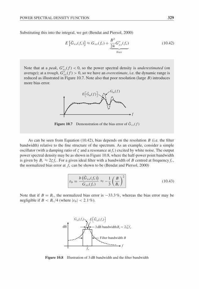
JWBK207-10 JWBK207-Shin January 18, 2008 8:20 Char Count= 0
POWER SPECTRAL DENSITY FUNCTION 329
Substituting this into the integral, we get (Bendat and Piersol, 2000)
E[Gxx ( fc)
] ≈ Gxx ( fc) + B2
24G ′′
xx ( fc)︸ ︷︷ ︸bias
(10.42)
Note that at a peak, G ′′xx ( f ) < 0, so the power spectral density is underestimated (on
average); at a trough, G ′′xx ( f ) > 0, so we have an overestimate, i.e. the dynamic range is
reduced as illustrated in Figure 10.7. Note also that poor resolution (large B) introducesmore bias error.
( )xxE G f( )xxG f
f
Figure 10.7 Demonstration of the bias error of Gxx ( f )
As can be seen from Equation (10.42), bias depends on the resolution B (i.e. the filterbandwidth) relative to the fine structure of the spectrum. As an example, consider a simpleoscillator (with a damping ratio of ζ and a resonance at fr ) excited by white noise. The outputpower spectral density may be as shown in Figure 10.8, where the half-power point bandwidthis given by Br ≈ 2ζ fr . For a given ideal filter with a bandwidth of B centred at frequency fr ,the normalized bias error at fr can be shown to be (Bendat and Piersol, 2000)
εb = b(Gxx ( fr )
)Gxx ( fr )
≈ −1
3
(B
Br
)2
(10.43)
Note that if B = Br , the normalized bias error is −33.3 %, whereas the bias error may benegligible if B < Br/4 (where |εb| < 2.1 %).
( )xx rE G f( )xx rG f
rf
3 dB bandwidth 2r rB fζ≈
Filter bandwidth B
f
dB
Figure 10.8 Illustration of 3 dB bandwidth and the filter bandwidth
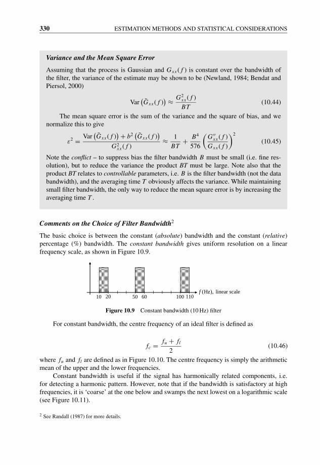
JWBK207-10 JWBK207-Shin January 18, 2008 8:20 Char Count= 0
330 ESTIMATION METHODS AND STATISTICAL CONSIDERATIONS
Variance and the Mean Square Error
Assuming that the process is Gaussian and Gxx ( f ) is constant over the bandwidth ofthe filter, the variance of the estimate may be shown to be (Newland, 1984; Bendat andPiersol, 2000)
Var(Gxx ( f )
) ≈ G2xx ( f )
BT(10.44)
The mean square error is the sum of the variance and the square of bias, and wenormalize this to give
ε2 = Var(Gxx ( f )
) + b2(Gxx ( f )
)G2
xx ( f )≈ 1
BT+ B4
576
(G ′′
xx ( f )
Gxx ( f )
)2
(10.45)
Note the conflict – to suppress bias the filter bandwidth B must be small (i.e. fine res-olution), but to reduce the variance the product BT must be large. Note also that theproduct BT relates to controllable parameters, i.e. B is the filter bandwidth (not the databandwidth), and the averaging time T obviously affects the variance. While maintainingsmall filter bandwidth, the only way to reduce the mean square error is by increasing theaveraging time T .
Comments on the Choice of Filter Bandwidth2
The basic choice is between the constant (absolute) bandwidth and the constant (relative)percentage (%) bandwidth. The constant bandwidth gives uniform resolution on a linearfrequency scale, as shown in Figure 10.9.
10 20 6050 110100(Hz), linear scalef
Figure 10.9 Constant bandwidth (10 Hz) filter
For constant bandwidth, the centre frequency of an ideal filter is defined as
fc = fu + fl
2(10.46)
where fu and fl are defined as in Figure 10.10. The centre frequency is simply the arithmeticmean of the upper and the lower frequencies.
Constant bandwidth is useful if the signal has harmonically related components, i.e.for detecting a harmonic pattern. However, note that if the bandwidth is satisfactory at highfrequencies, it is ‘coarse’ at the one below and swamps the next lowest on a logarithmic scale(see Figure 10.11).
2 See Randall (1987) for more details.
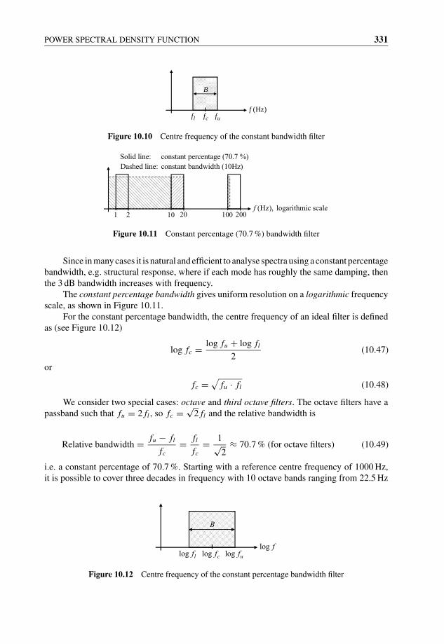
JWBK207-10 JWBK207-Shin January 18, 2008 8:20 Char Count= 0
POWER SPECTRAL DENSITY FUNCTION 331
(Hz)
B
flf cf uf
Figure 10.10 Centre frequency of the constant bandwidth filter
1 2 2010 200100(Hz), logarithmic scalef
Solid line: constant percentage (70.7 %)
Dashed line: constant bandwidth (10Hz)
Figure 10.11 Constant percentage (70.7 %) bandwidth filter
Since in many cases it is natural and efficient to analyse spectra using a constant percentagebandwidth, e.g. structural response, where if each mode has roughly the same damping, thenthe 3 dB bandwidth increases with frequency.
The constant percentage bandwidth gives uniform resolution on a logarithmic frequencyscale, as shown in Figure 10.11.
For the constant percentage bandwidth, the centre frequency of an ideal filter is definedas (see Figure 10.12)
log fc = log fu + log fl
2(10.47)
or
fc =√
fu · fl (10.48)
We consider two special cases: octave and third octave filters. The octave filters have apassband such that fu = 2 fl , so fc = √
2 fl and the relative bandwidth is
Relative bandwidth = fu − fl
fc= fl
fc= 1√
2≈ 70.7 % (for octave filters) (10.49)
i.e. a constant percentage of 70.7 %. Starting with a reference centre frequency of 1000 Hz,it is possible to cover three decades in frequency with 10 octave bands ranging from 22.5 Hz
B
log lf log cf log uflog f
Figure 10.12 Centre frequency of the constant percentage bandwidth filter
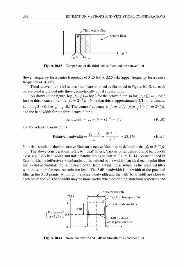
JWBK207-10 JWBK207-Shin January 18, 2008 8:20 Char Count= 0
332 ESTIMATION METHODS AND STATISTICAL CONSIDERATIONS
log lflog f
Third octave filter
Octave filter
log uf
Figure 10.13 Comparison of the third octave filter and the octave filter
(lower frequency for a centre frequency of 31.5 Hz) to 22.5 kHz (upper frequency for a centrefrequency of 16 kHz).
Third octave filters (1/3 octave filters) are obtained as illustrated in Figure 10.13, i.e. eachoctave band is divided into three geometrically equal subsections.
As shown in the figure, log ( fu/ fl) = log 2 for the octave filter, so log ( fu/ fl) = 13
log 2for the third octave filter, i.e. fu = 21/3 fl . (Note that this is approximately 1/10 of a decade,
i.e. 13
log 2 ≈ 0.1 = 110
log 10.) The centre frequency is fc = √fu · fl =
√21/3 f 2
l = 21/6 fl ,
and the bandwidth for the third octave filter is
Bandwidth = fu − fl = (21/3 − 1) fl (10.50)
and the relative bandwidth is
Relative bandwidth = fu − fl
fc= 21/3 − 1
21/6≈ 23.1 % (10.51)
Note that, similar to the third octave filter, an m octave filter may be defined so that fu = 21/m fl .The above considerations relate to ‘ideal’ filters. Various other definitions of bandwidth
exist, e.g. 3 dB bandwidth and noise bandwidth as shown in Figure 10.14. As mentioned inSection 4.6, the (effective) noise bandwidth is defined as the width of an ideal rectangular filterthat would accumulate the same noise power from a white noise source as the practical filterwith the same reference transmission level. The 3 dB bandwidth is the width of the practicalfilter at the 3 dB points. Although the noise bandwidth and the 3 dB bandwidth are close toeach other, the 3 dB bandwidth may be more useful when describing structural responses and
Practical band-pass filter
Noise bandwidth
1
0
0.5
Ideal band-pass filter
3 dB bandwidth of the practical filter
3 dBHalf power
( 3 dB)−
f
2( )H f
cf
Figure 10.14 Noise bandwidth and 3 dB bandwidth of a practical filter
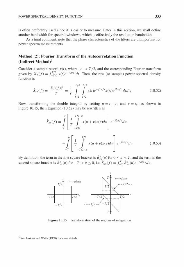
JWBK207-10 JWBK207-Shin January 18, 2008 8:20 Char Count= 0
POWER SPECTRAL DENSITY FUNCTION 333
is often preferably used since it is easier to measure. Later in this section, we shall defineanother bandwidth for spectral windows, which is effectively the resolution bandwidth.
As a final comment, note that the phase characteristics of the filters are unimportant forpower spectra measurements.
Method (2): Fourier Transform of the Autocorrelation Function
(Indirect Method)3
Consider a sample record x(t), where | t | < T/2, and the corresponding Fourier transform
given by XT ( f ) = ∫ T/2
−T/2x(t)e− j2π f t dt . Then, the raw (or sample) power spectral density
function is
Sxx ( f ) = |XT ( f )|2T
= 1
T
T/2∫−T/2
T/2∫−T/2
x(t)e− j2π f t x(t1)e j2π f t1 dtdt1 (10.52)
Now, transforming the double integral by setting u = t − t1 and v = t1, as shown inFigure 10.15, then Equation (10.52) may be rewritten as
Sxx ( f ) =T∫
0
⎡⎢⎣ 1
T
T /2−u∫−T /2
x(u + v)x(v)dv
⎤⎥⎦ e− j2π f udu
+0∫
−T
⎡⎢⎣ 1
T
T /2∫−T /2−u
x(u + v)x(v)dv
⎤⎥⎦ e− j2π f udu (10.53)
By definition, the term in the first square bracket is Rbxx (u) for 0 ≤ u < T , and the term in the
second square bracket is Rbxx (u) for −T < u ≤ 0, i.e. Sxx ( f ) = ∫ T
−T Rbxx (u)e− j2π f udu.
2T− 2T
2T
2T−
t
1t
1– -planet t– -planeu v
2T− 2T
2T
2T−
2u T v= −
2u T v= − −
u
v
T
T−
Figure 10.15 Transformation of the regions of integration
3 See Jenkins and Watts (1968) for more details.
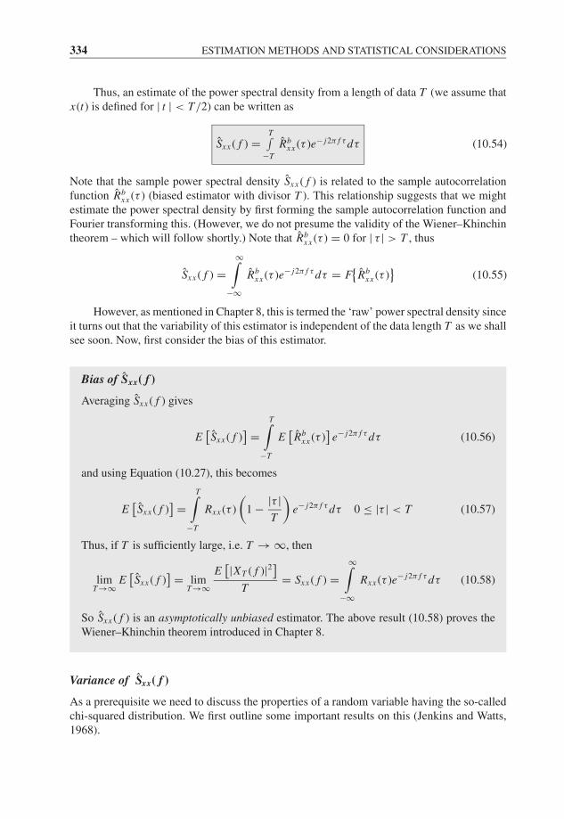
JWBK207-10 JWBK207-Shin January 18, 2008 8:20 Char Count= 0
334 ESTIMATION METHODS AND STATISTICAL CONSIDERATIONS
Thus, an estimate of the power spectral density from a length of data T (we assume thatx(t) is defined for | t | < T/2) can be written as
Sxx ( f ) =T∫
−TRb
xx (τ )e− j2π f τ dτ (10.54)
Note that the sample power spectral density Sxx ( f ) is related to the sample autocorrelationfunction Rb
xx (τ ) (biased estimator with divisor T ). This relationship suggests that we mightestimate the power spectral density by first forming the sample autocorrelation function andFourier transforming this. (However, we do not presume the validity of the Wiener–Khinchintheorem – which will follow shortly.) Note that Rb
xx (τ ) = 0 for | τ | > T , thus
Sxx ( f ) =∞∫
−∞Rb
xx (τ )e− j2π f τ dτ = F{
Rbxx (τ )
}(10.55)
However, as mentioned in Chapter 8, this is termed the ‘raw’ power spectral density sinceit turns out that the variability of this estimator is independent of the data length T as we shallsee soon. Now, first consider the bias of this estimator.
Bias of Sxx( f )
Averaging Sxx ( f ) gives
E[Sxx ( f )
] =T∫
−T
E[Rb
xx (τ )]
e− j2π f τ dτ (10.56)
and using Equation (10.27), this becomes
E[Sxx ( f )
] =T∫
−T
Rxx (τ )
(1 − |τ |
T
)e− j2π f τ dτ 0 ≤ |τ | < T (10.57)
Thus, if T is sufficiently large, i.e. T → ∞, then
limT →∞
E[Sxx ( f )
] = limT →∞
E[|XT ( f )|2]
T= Sxx ( f ) =
∞∫−∞
Rxx (τ )e− j2π f τ dτ (10.58)
So Sxx ( f ) is an asymptotically unbiased estimator. The above result (10.58) proves theWiener–Khinchin theorem introduced in Chapter 8.
Variance of Sxx( f )
As a prerequisite we need to discuss the properties of a random variable having the so-calledchi-squared distribution. We first outline some important results on this (Jenkins and Watts,1968).
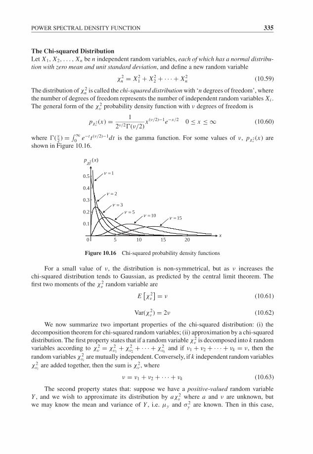
JWBK207-10 JWBK207-Shin January 18, 2008 8:20 Char Count= 0
POWER SPECTRAL DENSITY FUNCTION 335
The Chi-squared DistributionLet X1, X2, . . . , Xn be n independent random variables, each of which has a normal distribu-tion with zero mean and unit standard deviation, and define a new random variable
χ2n = X2
1 + X22 + · · · + X2
n (10.59)
The distribution of χ2n is called the chi-squared distribution with ‘n degrees of freedom’, where
the number of degrees of freedom represents the number of independent random variables Xi .The general form of the χ2
ν probability density function with ν degrees of freedom is
pχ2ν(x) = 1
2ν/2�(ν/2)x (ν/2)−1e−x/2 0 ≤ x ≤ ∞ (10.60)
where �( ν2) = ∫ ∞
0e−t t (ν/2)−1dt is the gamma function. For some values of ν, pχ2
ν(x) are
shown in Figure 10.16.
5 10 15 20
0.1
0.2
0.3
0.4
0.5
0
1ν =
2ν =
3ν =5ν =
10ν = 15ν =
2 ( )p xνχ
x
Figure 10.16 Chi-squared probability density functions
For a small value of ν, the distribution is non-symmetrical, but as ν increases thechi-squared distribution tends to Gaussian, as predicted by the central limit theorem. Thefirst two moments of the χ2
ν random variable are
E[χ2
ν
] = ν (10.61)
Var(χ2ν ) = 2ν (10.62)
We now summarize two important properties of the chi-squared distribution: (i) thedecomposition theorem for chi-squared random variables; (ii) approximation by a chi-squareddistribution. The first property states that if a random variable χ2
ν is decomposed into k randomvariables according to χ2
ν = χ2ν1
+ χ2ν2
+ · · · + χ2νk
and if ν1 + ν2 + · · · + νk = ν, then the
random variables χ2νi
are mutually independent. Conversely, if k independent random variables
χ2νi
are added together, then the sum is χ2ν , where
ν = ν1 + ν2 + · · · + νk (10.63)
The second property states that: suppose we have a positive-valued random variableY , and we wish to approximate its distribution by aχ2
ν where a and ν are unknown, butwe may know the mean and variance of Y , i.e. μy and σ 2
y are known. Then in this case,

JWBK207-10 JWBK207-Shin January 18, 2008 8:20 Char Count= 0
336 ESTIMATION METHODS AND STATISTICAL CONSIDERATIONS
E [Y ] = μy = E[aχ2ν ] = aν and σ 2
y = Var(aχ2ν ) = a2Var(χ2
ν ) = 2a2ν = 2μ2y/ν. Thus a and
ν are found from
a = μy
ν(10.64)
ν = 2μ2y
σ 2y
(10.65)
Variance ConsiderationsWe now return to study the variance of Sxx ( f ). The sample power spectral density functioncan be written as (x(t) is defined for | t | < T/2)
Sxx ( f ) = |XT ( f )|2T
= 1
T
∣∣∣∣∣∣∣T /2∫
−T /2
x(t)e− j2π f t dt
∣∣∣∣∣∣∣2
= 1
T
∣∣∣∣∣∣∞∫
−∞x(t)e− j2π f t dt
∣∣∣∣∣∣2
= 1
T
⎧⎪⎨⎪⎩⎡⎣ ∞∫
−∞x(t) cos(2π f t)dt
⎤⎦2
+⎡⎣ ∞∫
−∞x(t) sin(2π f t)dt
⎤⎦2⎫⎪⎬⎪⎭
= 1
T
[X2
c ( f ) + X2s ( f )
](10.66)
where Xc( f ) and Xs( f ) are Fourier cosine and sine transforms of x(t).Let us assume that x(t) is a Gaussian process with zero mean value; then Xc( f )
and Xs( f ) are also Gaussian and have zero mean values. Furthermore, it can be shownthat Xc( f ) and Xs( f ) are uncorrelated and have approximately equal variances (Jenkinsand Watts, 1968). Now if the variances were unity, we could use the properties of thechi-squared distribution to say Sxx ( f ) is related to a χ2
2 distribution (note that Sxx ( f ) isa squared quantity and so positive valued). We do this as follows. Let
1
TE
[X2
c ( f )] = 1
TE
[X2
s ( f )] = σ 2 (say, for each frequency f ) (10.67)
and
E[Sxx ( f )
] ≈ Sxx ( f ) = 2σ 2 (10.68)
Then, it can be shown that
2Sxx ( f )
Sxx ( f )= X2
c ( f )
T σ 2+ X2
s ( f )
T σ 2(10.69)
which is the sum of two squared Gaussian random variables with unit variances (note thatXc( f ) and Xs( f ) are jointly normally distributed (see Appendix G for justification) anduncorrelated, so they are independent). Therefore the random variable 2Sxx ( f )/Sxx ( f )
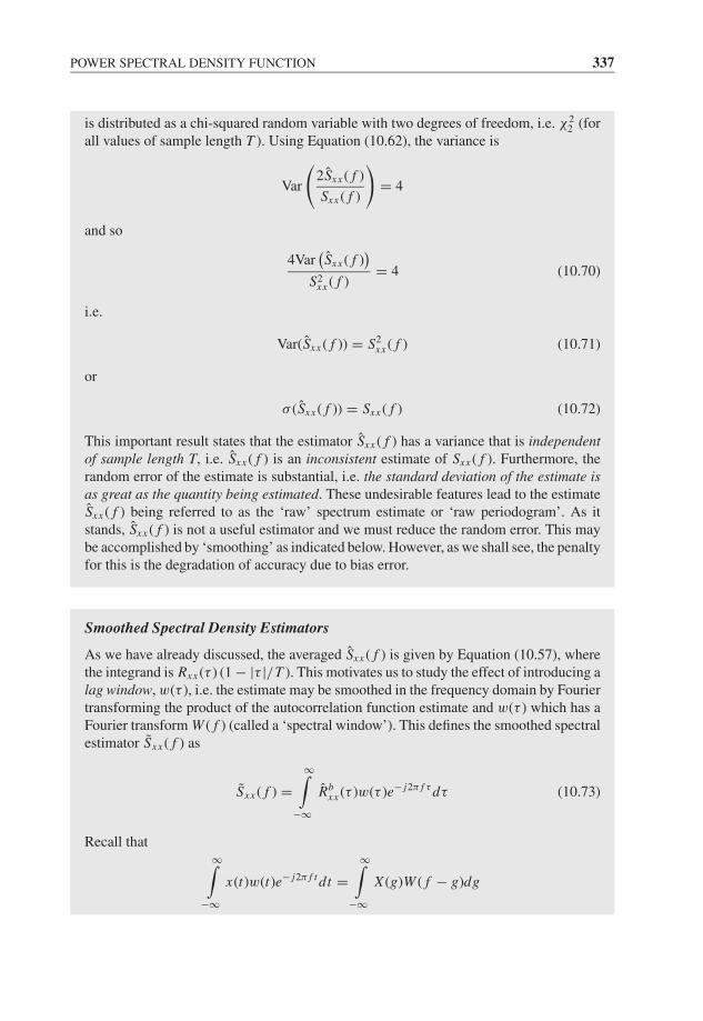
JWBK207-10 JWBK207-Shin January 18, 2008 8:20 Char Count= 0
POWER SPECTRAL DENSITY FUNCTION 337
is distributed as a chi-squared random variable with two degrees of freedom, i.e. χ22 (for
all values of sample length T ). Using Equation (10.62), the variance is
Var
(2Sxx ( f )
Sxx ( f )
)= 4
and so
4Var(Sxx ( f )
)S2
xx ( f )= 4 (10.70)
i.e.
Var(Sxx ( f )) = S2xx ( f ) (10.71)
or
σ (Sxx ( f )) = Sxx ( f ) (10.72)
This important result states that the estimator Sxx ( f ) has a variance that is independentof sample length T, i.e. Sxx ( f ) is an inconsistent estimate of Sxx ( f ). Furthermore, therandom error of the estimate is substantial, i.e. the standard deviation of the estimate isas great as the quantity being estimated. These undesirable features lead to the estimateSxx ( f ) being referred to as the ‘raw’ spectrum estimate or ‘raw periodogram’. As itstands, Sxx ( f ) is not a useful estimator and we must reduce the random error. This maybe accomplished by ‘smoothing’ as indicated below. However, as we shall see, the penaltyfor this is the degradation of accuracy due to bias error.
Smoothed Spectral Density Estimators
As we have already discussed, the averaged Sxx ( f ) is given by Equation (10.57), wherethe integrand is Rxx (τ ) (1 − |τ |/T ). This motivates us to study the effect of introducing alag window, w(τ ), i.e. the estimate may be smoothed in the frequency domain by Fouriertransforming the product of the autocorrelation function estimate and w(τ ) which has aFourier transform W ( f ) (called a ‘spectral window’). This defines the smoothed spectralestimator Sxx ( f ) as
Sxx ( f ) =∞∫
−∞Rb
xx (τ )w(τ )e− j2π f τ dτ (10.73)
Recall that∞∫
−∞x(t)w(t)e− j2π f t dt =
∞∫−∞
X (g)W ( f − g)dg

JWBK207-10 JWBK207-Shin January 18, 2008 8:20 Char Count= 0
338 ESTIMATION METHODS AND STATISTICAL CONSIDERATIONS
i.e. Sxx ( f ) = Sxx ( f ) ∗ W ( f ), which is the convolution of the raw spectral density witha spectral window. Thus the right hand side of Equation (10.73) has an alternative form
Sxx ( f ) =∞∫
−∞Sxx (g)W ( f − g)dg (10.74)
This estimation procedure may be viewed as a smoothing operation in the frequencydomain. Thus the lag window w(τ ) results in the spectral window W ( f ) ‘smoothing’ theraw periodogram Sxx ( f ) through the convolution operation. In fact, the above method isthe basis of the correlation method of estimating spectral density functions. In the timedomain, the lag window can be regarded as reducing the ‘importance’ of values of Rb
xx (τ )as τ increases.
It is necessary to start all over again and study the bias and variance properties of thisnew estimator Sxx ( f ) where clearly the window function w(τ ) will now play an importantrole. Jenkins and Watts (1968) and Priestley (1981) give a detailed discussion of this problem.We shall only quote the main results here.
Some commonly used window functions are listed in Table 10.1. The rectangular windowis included for completeness, and other window functions may also be used. Note that thediscussions on window functions given in Chapter 4 are directly related to this case.
The lag windows w(τ ) are shown in Figure 10.17, where w(0) = 1 for all windows,and the spectral windows W ( f ) are shown in Figure 10.18. Note that the spectral win-dows which take negative values might give rise to negative spectral density estimates in thisapproach.
Table 10.1 Commonly used lag and spectral windows
Windowname Lag window, w(τ ) Spectral window, W ( f )
Rectangularw(τ ) = 1
= 0
|τ | ≤ Tw
|τ | > Tw
W ( f ) = 2Tw
(sin(2π f Tw)
2π f Tw
)
Bartlettw(τ ) = 1 − |τ |
Tw= 0
|τ | ≤ Tw
|τ | > Tw
W ( f ) = Tw
(sin(π f Tw)
π f Tw
)2
Hann(ing)w(τ ) = 1
2
(1 + cos
πτ
Tw
)= 0
|τ | ≤ Tw
|τ | > Tw
W ( f ) = Tw
(sin(2π f Tw)
2π f Tw
)1
1 − (2 f Tw)2
Hammingw(τ ) = 0.54 + 0.46 cos
πτ
Tw= 0
|τ | ≤ Tw
|τ | > Tw
W ( f ) =[0.54π2 − 0.08(2π f Tw)2
]sin(2π f Tw)
2π f Tw
[π2 − (2π f Tw)2
]
Parzen
w(τ ) = 1 − 6
(τ
Tw
)2
+ 6
( |τ |Tw
)3
= 2
(1 − |τ |
Tw
)3
= 0
|τ | ≤ Tw
2Tw
2< |τ | ≤ Tw
|τ | > Tw
W ( f ) = 3
4Tw
(sin(π f Tw/2)
π f Tw/2
)4
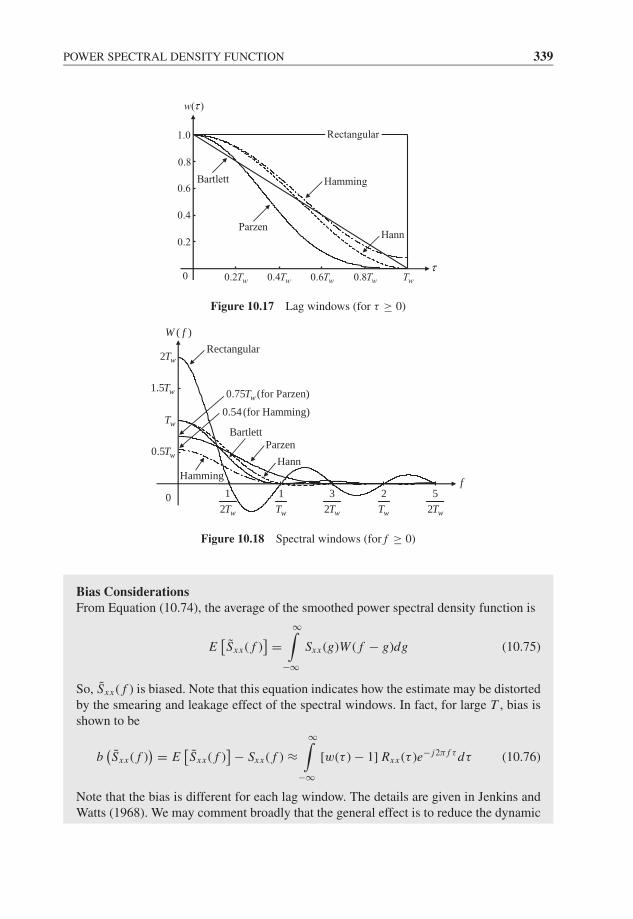
JWBK207-10 JWBK207-Shin January 18, 2008 8:20 Char Count= 0
POWER SPECTRAL DENSITY FUNCTION 339
( )w τ
τ0.2 wT0 0.4 wT 0.6 wT 0.8 wT wT
0.2
0.4
0.6
0.8
1.0 Rectangular
Hamming
Hann
Bartlett
Parzen
Figure 10.17 Lag windows (for τ ≥ 0)
( )W f
1
wT
2
wT
2 wT
32 wT
52 wT
12 wT
1.5 wT
wT
0.5 wT
0.54(for Hamming)
0.75 (for Parzen)wT
fHamming
Hann
ParzenBartlett
Rectangular
0
Figure 10.18 Spectral windows (for f ≥ 0)
Bias ConsiderationsFrom Equation (10.74), the average of the smoothed power spectral density function is
E[Sxx ( f )
] =∞∫
−∞Sxx (g)W ( f − g)dg (10.75)
So, Sxx ( f ) is biased. Note that this equation indicates how the estimate may be distortedby the smearing and leakage effect of the spectral windows. In fact, for large T , bias isshown to be
b(Sxx ( f )
) = E[Sxx ( f )
] − Sxx ( f ) ≈∞∫
−∞[w(τ ) − 1] Rxx (τ )e− j2π f τ dτ (10.76)
Note that the bias is different for each lag window. The details are given in Jenkins andWatts (1968). We may comment broadly that the general effect is to reduce the dynamic
JWBK207-10 JWBK207-Shin January 18, 2008 8:20 Char Count= 0
340 ESTIMATION METHODS AND STATISTICAL CONSIDERATIONS
range of the spectra as in the filter bank method of the spectral estimation, i.e. peaks areunderestimated and troughs are overestimated.
As can be seen from Equation (10.75), the bias is reduced as the spectral windowgets narrower, i.e. as the width of the lag window w(τ ) gets larger, the spectral windowbecomes W ( f ) → δ( f ). So, Sxx ( f ) is asymptotically unbiased (for Tw → ∞). However,the spectral windows cannot be made too narrow since then there is little smoothing andthe random errors increase, so we need W ( f ) to have some width to do the smoothing.Consequently, once again we need a compromise between bias and variance, i.e. a trade-off between the resolution and the random error. Note that, sometimes, the bias problemis referred to under ‘bandwidth considerations’ since small bias is associated with smallbandwidth of the window function.
Variance ConsiderationsFrom Equation (10.74), Sxx ( f ) can be considered as a weighted sum of values of Sxx ( f ).Thus, it may be argued that nSxx ( f )/Sxx ( f ) is approximately distributed as a chi-squaredrandom variable with n degrees of freedom, χ2
n , where the number of degrees of freedomis defined as
n = 2T∫ ∞−∞ w2(τ )dτ
= 2T
I(10.77)
which depends on the window and data length (Jenkins and Watts, 1968).Also, since Var(nSxx ( f )/Sxx ( f )) = 2n, it can be shown that
Var(Sxx ( f )) = S2xx ( f )
n/2= S2
xx ( f )
T/I(10.78)
σ (Sxx ( f )) = Sxx ( f )√n/2
= Sxx ( f )√T/I
(10.79)
Now, 1/I can be argued to be a measure of the resolution bandwidth B of the window(see below for justification), so the number of degrees of freedom is n = 2BT . Thus, theabove equations can be rewritten as
Var(Sxx ( f ))
S2xx ( f )
= 1
BT(10.80)
σ (Sxx ( f ))
Sxx ( f )= 1√
BT(10.81)
To justify that 1/I is a measure of bandwidth, consider an ideal filter shown in Figure 10.19,where
I =∞∫
−∞w2(τ )dτ =
∞∫−∞
W 2( f )d f (10.82)
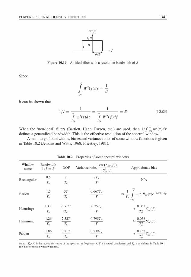
JWBK207-10 JWBK207-Shin January 18, 2008 8:20 Char Count= 0
POWER SPECTRAL DENSITY FUNCTION 341
2B
1 B
( )W f
f
B
Figure 10.19 An ideal filter with a resolution bandwidth of B
Since
∞∫−∞
W 2( f )d f = 1
B
it can be shown that
1/I = 1∞∫
−∞w2(τ )dτ
= 1∞∫
−∞W 2( f )d f
= B (10.83)
When the ‘non-ideal’ filters (Bartlett, Hann, Parzen, etc.) are used, then 1/∫ ∞−∞ w2(τ )dτ
defines a generalized bandwidth. This is the effective resolution of the spectral window.A summary of bandwidths, biases and variance ratios of some window functions is given
in Table 10.2 (Jenkins and Watts, 1968; Priestley, 1981).
Table 10.2 Properties of some spectral windows
Window Bandwidthname 1/I = B DOF Variance ratio,
Var(Sxx ( f )
)S2
xx ( f )Approximate bias
Rectangular0.5
Tw
T
Tw
2Tw
TN/A
Barlett1.5
Tw
3T
Tw
0.667Tw
T≈ 1
Tw
∞∫−∞
−|τ |Rxx (τ )e− j2π f τ dτ
Hann(ing)1.333
Tw
2.667T
Tw
0.75Tw
T≈ 0.063
T 2w
S′′xx ( f )
Hamming1.26
Tw
2.52T
Tw
0.795Tw
T≈ 0.058
T 2w
S′′xx ( f )
Parzen1.86
Tw
3.71T
Tw
0.539Tw
T≈ 0.152
T 2w
S′′xx ( f )
Note: S′′xx ( f ) is the second derivative of the spectrum at frequency f , T is the total data length and Tw is as defined in Table 10.1
(i.e. half of the lag window length).
JWBK207-10 JWBK207-Shin January 18, 2008 8:20 Char Count= 0
342 ESTIMATION METHODS AND STATISTICAL CONSIDERATIONS
General Comments on Window Functions and Sxx( f )
Although the rectangular window is included in Table 10.2, it is rarely used since its spectralwindow side lobes cause large ‘leakage’ effects. However, in Chapter 8, the rectangular windowfunction is applied to estimate the spectral density functions in MATLAB Examples 8.8–8.10(note that we have used a very long data length T ).
Bias of the Bartlett window is of order 1/Tw and so will in general be greater than otherwindows (order 1/T 2
w). Among the Hann, Hamming and Parzen windows, the Parzen windowhas the smallest variance but has the greatest bias. Since the bias of these windows depends onS′′
xx ( f ), larger bias occurs at sharp peaks and troughs than other frequency regions. From thetable, we can easily see that the bias is reduced as Tw increases, but the variance is increased.The variance can then be reduced by increasing the total data length T .
We note that: (i) when the bias is small, Sxx ( f ) is said to reproduce Sxx ( f ) with highfidelity; (ii) when the variance is small, the estimator is said to have high stability (Jenkins andWatts, 1968). The choice of window functions should depend on whether the concern is forstatistical stability (low variance) or high fidelity (small bias), although in general we mustconsider both. For example, if the spectral density function has narrow peaks of importancewe may willingly tolerate some loss of stability to resolve the peak properly, while if thespectral density function is smooth then bias errors are not likely to be so important. Thus, wemay state that the estimator Sxx ( f ) is approximately unbiased and has a low variance only ifthe sufficiently narrow resolution bandwidth and yet long enough data are used.
When spectra are estimated via the autocorrelation function many texts give only ap-proximate values for the degrees of freedom and the resolution bandwidth. For example, withdigital analysis with N data points (sampled at every seconds) and a maximum correlationlag M , the number of degrees of freedom is usually quoted as 2N/M and the resolutionbandwidth as 1/(M) (this may corresponds to the rectangular window function).
Finally, instead of multiplying the sample autocorrelation function by the lag window andFourier transforming the weighted sample autocorrelation function, an alternative procedureis to do the smoothing in the frequency domain, i.e. form the raw periodogram and performthe frequency convolution. This ‘frequency smoothing’ will be referred to again soon.
Method (3): Direct Methods
We shall now discuss the basis for forming smoothed power spectral density estimates withoutfirst forming the autocorrelation functions. These methods are probably the most widelyused because of computational considerations. There are two methods, although they can becombined if required, namely (i) segment averaging; (ii) frequency smoothing.
Segment Averaging (Welch’s Method)M10.1
The segment averaging method has become very popular mainly because of its fastspeed of computation. The method is discussed in Jenkins and Watts (1968) as Bartlett’ssmoothing procedure and in Welch (1967) in some detail. The basic procedure is outlinedwith reference to Figure 10.20.
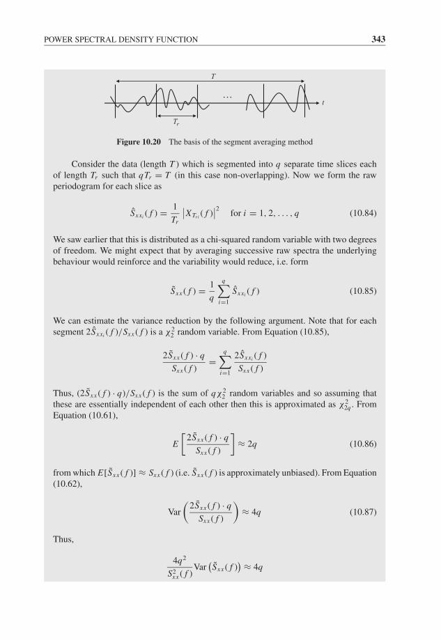
JWBK207-10 JWBK207-Shin January 18, 2008 8:20 Char Count= 0
POWER SPECTRAL DENSITY FUNCTION 343
t
T
rT
Figure 10.20 The basis of the segment averaging method
Consider the data (length T ) which is segmented into q separate time slices eachof length Tr such that qTr = T (in this case non-overlapping). Now we form the rawperiodogram for each slice as
Sxxi ( f ) = 1
Tr
∣∣XTri ( f )∣∣2
for i = 1, 2, . . . , q (10.84)
We saw earlier that this is distributed as a chi-squared random variable with two degreesof freedom. We might expect that by averaging successive raw spectra the underlyingbehaviour would reinforce and the variability would reduce, i.e. form
Sxx ( f ) = 1
q
q∑i=1
Sxxi ( f ) (10.85)
We can estimate the variance reduction by the following argument. Note that for eachsegment 2Sxxi ( f )/Sxx ( f ) is a χ2
2 random variable. From Equation (10.85),
2Sxx ( f ) · q
Sxx ( f )=
q∑i=1
2Sxxi ( f )
Sxx ( f )
Thus, (2Sxx ( f ) · q)/Sxx ( f ) is the sum of qχ22 random variables and so assuming that
these are essentially independent of each other then this is approximated as χ22q . From
Equation (10.61),
E
[2Sxx ( f ) · q
Sxx ( f )
]≈ 2q (10.86)
from which E[Sxx ( f )] ≈ Sxx ( f ) (i.e. Sxx ( f ) is approximately unbiased). From Equation(10.62),
Var
(2Sxx ( f ) · q
Sxx ( f )
)≈ 4q (10.87)
Thus,
4q2
S2xx ( f )
Var(Sxx ( f )
) ≈ 4q
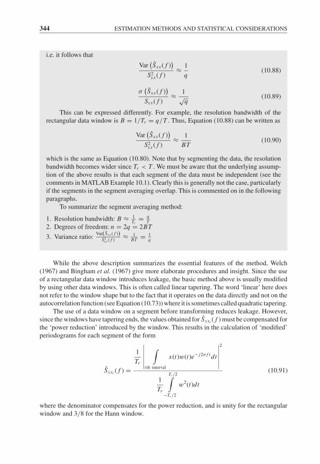
JWBK207-10 JWBK207-Shin January 18, 2008 8:20 Char Count= 0
344 ESTIMATION METHODS AND STATISTICAL CONSIDERATIONS
i.e. it follows that
Var(Sxx ( f )
)S2
xx ( f )≈ 1
q(10.88)
σ(Sxx ( f )
)Sxx ( f )
≈ 1√q
(10.89)
This can be expressed differently. For example, the resolution bandwidth of therectangular data window is B = 1/Tr = q/T . Thus, Equation (10.88) can be written as
Var(Sxx ( f )
)S2
xx ( f )≈ 1
BT(10.90)
which is the same as Equation (10.80). Note that by segmenting the data, the resolutionbandwidth becomes wider since Tr < T . We must be aware that the underlying assump-tion of the above results is that each segment of the data must be independent (see thecomments in MATLAB Example 10.1). Clearly this is generally not the case, particularlyif the segments in the segment averaging overlap. This is commented on in the followingparagraphs.
To summarize the segment averaging method:
1. Resolution bandwidth: B ≈ 1Tr
= qT
2. Degrees of freedom: n = 2q = 2BT
3. Variance ratio:Var(Sxx ( f ))
S2xx ( f )
≈ 1BT = 1
q
While the above description summarizes the essential features of the method, Welch(1967) and Bingham et al. (1967) give more elaborate procedures and insight. Since the useof a rectangular data window introduces leakage, the basic method above is usually modifiedby using other data windows. This is often called linear tapering. The word ‘linear’ here doesnot refer to the window shape but to the fact that it operates on the data directly and not on theautocorrelation function (see Equation (10.73)) where it is sometimes called quadratic tapering.
The use of a data window on a segment before transforming reduces leakage. However,since the windows have tapering ends, the values obtained for Sxxi ( f ) must be compensated forthe ‘power reduction’ introduced by the window. This results in the calculation of ‘modified’periodograms for each segment of the form
Sxxi ( f ) =
1
Tr
∣∣∣∣∣∣∫
i th interval
x(t)w(t)e− j2π f t dt
∣∣∣∣∣∣2
1
Tr
Tr /2∫−Tr /2
w2(t)dt
(10.91)
where the denominator compensates for the power reduction, and is unity for the rectangularwindow and 3/8 for the Hann window.
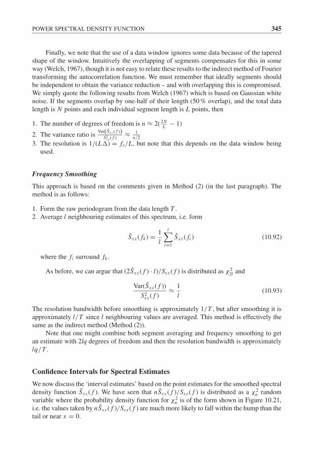
JWBK207-10 JWBK207-Shin January 18, 2008 8:20 Char Count= 0
POWER SPECTRAL DENSITY FUNCTION 345
Finally, we note that the use of a data window ignores some data because of the taperedshape of the window. Intuitively the overlapping of segments compensates for this in someway (Welch, 1967), though it is not easy to relate these results to the indirect method of Fouriertransforming the autocorrelation function. We must remember that ideally segments shouldbe independent to obtain the variance reduction – and with overlapping this is compromised.We simply quote the following results from Welch (1967) which is based on Gaussian whitenoise. If the segments overlap by one-half of their length (50 % overlap), and the total datalength is N points and each individual segment length is L points, then
1. The number of degrees of freedom is n ≈ 2( 2NL − 1)
2. The variance ratio isVar(Sxx ( f ))
S2xx ( f )
≈ 1n/2
3. The resolution is 1/(L) = fs/L , but note that this depends on the data window beingused.
Frequency Smoothing
This approach is based on the comments given in Method (2) (in the last paragraph). Themethod is as follows:
1. Form the raw periodogram from the data length T .2. Average l neighbouring estimates of this spectrum, i.e. form
Sxx ( fk) = 1
l
l∑i=1
Sxx ( fi ) (10.92)
where the fi surround fk .
As before, we can argue that (2Sxx ( f ) · l)/Sxx ( f ) is distributed as χ22l and
Var(Sxx ( f ))
S2xx ( f )
≈ 1
l(10.93)
The resolution bandwidth before smoothing is approximately 1/T , but after smoothing it isapproximately l/T since l neighbouring values are averaged. This method is effectively thesame as the indirect method (Method (2)).
Note that one might combine both segment averaging and frequency smoothing to getan estimate with 2lq degrees of freedom and then the resolution bandwidth is approximatelylq/T .
Confidence Intervals for Spectral Estimates
We now discuss the ‘interval estimates’ based on the point estimates for the smoothed spectraldensity function Sxx ( f ). We have seen that nSxx ( f )/Sxx ( f ) is distributed as a χ2
n randomvariable where the probability density function for χ2
n is of the form shown in Figure 10.21,i.e. the values taken by nSxx ( f )/Sxx ( f ) are much more likely to fall within the hump than thetail or near x = 0.
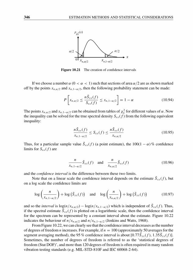
JWBK207-10 JWBK207-Shin January 18, 2008 8:20 Char Count= 0
346 ESTIMATION METHODS AND STATISTICAL CONSIDERATIONS
,1 2nx α−
2 (x)n
pχ
2α2α
, 2nx αx
0
Figure 10.21 The creation of confidence intervals
If we choose a number α (0 < α < 1) such that sections of area α/2 are as shown markedoff by the points xn,α/2 and xn,1−α/2, then the following probability statement can be made:
P
[xn,α/2 ≤ nSxx ( f )
Sxx ( f )≤ xn,1−α/2
]= 1 − α (10.94)
The points xn,α/2 and xn,1−α/2 can be obtained from tables of χ2n for different values of α. Now
the inequality can be solved for the true spectral density Sxx ( f ) from the following equivalentinequality:
nSxx ( f )
xn,1−α/2
≤ Sxx ( f ) ≤ nSxx ( f )
xn,α/2
(10.95)
Thus, for a particular sample value Sxx ( f ) (a point estimate), the 100(1 − α) % confidencelimits for Sxx ( f ) are
n
xn,1−α/2
Sxx ( f ) andn
xn,α/2
Sxx ( f ) (10.96)
and the confidence interval is the difference between these two limits.Note that on a linear scale the confidence interval depends on the estimate Sxx ( f ), but
on a log scale the confidence limits are
log
(n
xn,1−α/2
)+ log
(Sxx ( f )
)and log
(n
xn,α/2
)+ log
(Sxx ( f )
)(10.97)
and so the interval is log(n/xn,α/2) − log(n/xn,1−α/2) which is independent of Sxx ( f ). Thus,if the spectral estimate Sxx ( f ) is plotted on a logarithmic scale, then the confidence intervalfor the spectrum can be represented by a constant interval about the estimate. Figure 10.22indicates the behaviour of n/xn,α/2 and n/xn,1−α/2 (Jenkins and Watts, 1968).
From Figure 10.22, we can clearly see that the confidence interval decreases as the numberof degrees of freedom n increases. For example, if n = 100 (approximately 50 averages for thesegment averaging method), the 95 % confidence interval is about [0.77Sxx ( f ), 1.35Sxx ( f )].Sometimes, the number of degrees of freedom is referred to as the ‘statistical degrees offreedom (Stat DOF)’, and more than 120 degrees of freedom is often required in many randomvibration testing standards (e.g. MIL-STD-810F and IEC 60068-2-64).

JWBK207-10 JWBK207-Shin January 18, 2008 8:20 Char Count= 0
CROSS-SPECTRAL DENSITY FUNCTIONM10.1,10.3 347
001014 6 8 20 30 40 60 800.2
0.3
0.4
0.6
0.8
1
2
3
4
6
8
10
, 2n
n
x α
,1 2n
n
x α−
99%
95%
90%
99%
95%
90%
n (degrees of freedom)
1.35
0.77
80%
80%
0.5
0.7
0.9
5
7
9
0705975 90
Figure 10.22 Confidence interval limits
10.5 CROSS-SPECTRAL DENSITY FUNCTIONM10.1,10.3
The basic considerations given in Section 10.4 relate also to cross-spectral density functionestimation together with some additional features, but we shall not go into any detail here.Detailed results can be found in Jenkins and Watts (1968). We shall merely summarize someimportant features.
The raw cross-spectral density function can be obtained by Fourier transforming the rawcross-correlation function, i.e.
Sxy( f ) =T∫
−T
Rbxy(τ )e− j2π f τ dτ (10.98)
and this has the same unsatisfactory properties as the raw power spectral density function.Thus, as before, a lag window w(τ ) is introduced to smooth the estimate, i.e.
Sxy( f ) =T∫
−T
Rbxy(τ )w(τ )e− j2π f τ dτ (10.99)

JWBK207-10 JWBK207-Shin January 18, 2008 8:20 Char Count= 0
348 ESTIMATION METHODS AND STATISTICAL CONSIDERATIONS
Note that the unbiased estimator Rxy(τ ) may also be used in place of Rbxy(τ ) provided that the
maximum lag τmax is relatively small compared with T . Alternatively, the smoothed estimatecan be obtained by the segment averaging method or by frequency smoothing of the raw cross-spectral density. For example, if the segment averaging method is used the raw and smoothedcross-spectral density functions are
Sxyi ( f ) = 1
Tr
[X*
Tri( f )YTri ( f )
]for i = 1, 2, . . . , q (10.100)
Sxy( f ) = 1
q
q∑i=1
Sxyi ( f ) (10.101)
The smoothed estimate Sxy( f ) may be written in the form
Sxy( f ) = ∣∣Sxy( f )∣∣ e j arg Sxy ( f ) (10.102)
Roughly speaking, one can show that the variances of the amplitude∣∣Sxy( f )
∣∣ and thephase arg Sxy( f ) are proportional to 1/BT where B is the resolution bandwidth and Tis the data length.
Whilst the general effect of smoothing is much the same as for the power spectraldensity estimate, we note in addition, though, that the amplitude and phase estimatorsare also strongly dependent on the ‘true’ coherence function γ 2
xy( f ). So, as Jenkins andWatts (1968) observed, the sampling properties of the amplitude and phase estimatorsmay be dominated by the ‘uncontrollable’ influence of the coherence spectrum γ 2
xy( f )rather than by the ‘controllable’ influence of the smoothing factor 1/BT . For example,the variance of the modulus and phase of Sxy( f ) are shown to be (Bendat and Piersol,2000)
Var(∣∣Sxy( f )
∣∣)∣∣Sxy( f )∣∣2
≈ 1
γ 2xy( f )
· 1
BT(10.103)
Var(arg Sxy( f )
) ≈ 1 − γ 2xy( f )
γ 2xy( f )
· 1
2BT(10.104)
Note the ‘uncontrollable’ influence of true coherence function γ 2xy( f ) on the variability
of the estimate. Note also that the variance of arg Sxy( f ) is not normalized. Particularly,if x(t) and y(t) are fully linearly related, i.e. γ 2
xy( f ) = 1, then Var(arg Sxy( f )) ≈ 0. Thus,we see that the random error of the phase estimator is much smaller than that of theamplitude estimator.
Similar to the power spectral density estimate, in general, the estimator Sxy( f )is approximately unbiased when T is sufficiently large and the resolution bandwidthis narrow. However, there is another important aspect: since Rxy(τ ) is not (in general)symmetric, it is necessary to ensure that its maximum is well within the window w(τ )or serious bias errors result. For example, if y(t) = x(t − ), then it can be shown that

JWBK207-10 JWBK207-Shin January 18, 2008 8:20 Char Count= 0
COHERENCE FUNCTION 349
(Schmidt, 1985b) for rectangular windows
E[Sxy( f )
] ≈(
1 −
Tr
)Sxy( f ) (10.105)
where Tr is the length of window (or the length of segment). Note that the time delaybetween signals results in biased estimates (see MATLAB Example 10.3). This problemmay be avoided by ‘aligning’ the two time series so that the cross-correlation functionRxy(τ ) has a maximum at τ = 0.
10.6 COHERENCE FUNCTIONM10.2
The estimate for the coherence function is made up from the estimates of the smoothed powerand cross-spectral density functions as
γ 2xy( f ) =
∣∣Sxy( f )∣∣2
Sxx ( f )S yy( f )(10.106)
It should be noted that if ‘raw’ spectral density functions are used on the right hand side of theequation, it can be easily verified that the sample coherence function γ 2
xy( f ) is always ‘unity’for all frequencies for any signals x and y (even if they are unrelated).
Detailed calculations are given in Jenkins and Watts (1968) for the sampling propertiesof the smoothed coherence function γ 2
xy( f ), but roughly speaking, the variance of γ 2xy( f ) is
proportional to 1/BT (which is known, so a controllable parameter) and also depends onγ 2
xy( f ) (which is unknown, so is an uncontrollable parameter), where the variance of γ 2xy( f )
is shown to be
Var(γ 2
xy( f ))(
γ 2xy( f )
)2≈ 2
(1 − γ 2
xy( f ))2
γ 2xy( f )
· 1
BT(10.107)
This expression is sometimes used as an approximate guide after measurements have beenmade by replacing γ 2
xy( f ) with γ 2xy( f ).
Jenkins and Watts (1968) show that the bias of this estimator is proportional to the squareof the derivative of the phase spectrum arg Sxy( f ). For example, if the Hann window is usedthe normalized bias error can be expressed by
b(γ 2
xy( f ))
γ 2xy( f )
≈ −0.126
T 2w
(d
d f
(arg Sxy( f )
))2
(10.108)
for large T (total data length), where Tw is half of the lag window length as defined inTable 10.1. For the Parzen window, 0.126 is replaced by 0.304. The above equation meansthat the estimator is sensitive to delays between x(t) and y(t). Similar to the cross-spectraldensity function estimate, such bias can be reduced by realigning the processes, i.e. aligningthe peak in the cross-correlation between x(t) and y(t) to occur at zero lag.
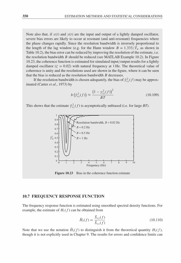
JWBK207-10 JWBK207-Shin January 18, 2008 8:20 Char Count= 0
350 ESTIMATION METHODS AND STATISTICAL CONSIDERATIONS
Note also that, if x(t) and y(t) are the input and output of a lightly damped oscillator,severe bias errors are likely to occur at resonant (and anti-resonant) frequencies wherethe phase changes rapidly. Since the resolution bandwidth is inversely proportional tothe length of the lag window (e.g. for the Hann window B = 1.333/Tw as shown inTable 10.2), the bias error can be reduced by improving the resolution of the estimate, i.e.the resolution bandwidth B should be reduced (see MATLAB Example 10.2). In Figure10.23, the coherence function is estimated for simulated input/output results for a lightlydamped oscillator (ζ = 0.02) with natural frequency at 1 Hz. The theoretical value ofcoherence is unity and the resolutions used are shown in the figure, where it can be seenthat the bias is reduced as the resolution bandwidth B decreases.
If the resolution bandwidth is chosen adequately, the bias of γ 2xy( f ) may be approx-
imated (Carter et al., 1973) by
b(γ 2
xy( f )) ≈
(1 − γ 2
xy( f ))2
BT(10.109)
This shows that the estimate γ 2xy( f ) is asymptotically unbiased (i.e. for large BT).
2xyγ
Resolution bandwidth, B ≈ 0.02 Hz
B ≈ 0.2 Hz
B ≈ 0.5 Hz
B ≈ 1 Hz
0 1 2 3 4 5 6 7 8 9 100
0.1
0.2
0.3
0.4
0.5
0.6
0.7
0.8
0.9
1
Frequency (Hz)
Figure 10.23 Bias in the coherence function estimate
10.7 FREQUENCY RESPONSE FUNCTION
The frequency response function is estimated using smoothed spectral density functions. Forexample, the estimate of H1( f ) can be obtained from
H1( f ) = Sxy( f )
Sxx ( f )(10.110)
Note that we use the notation H1( f ) to distinguish it from the theoretical quantity H1( f ),though it is not explicitly used in Chapter 9. The results for errors and confidence limits can
JWBK207-10 JWBK207-Shin January 18, 2008 8:20 Char Count= 0
FREQUENCY RESPONSE FUNCTION 351
be found in Bendat and Piersol (1980, 2000) and Otnes and Enochson (1978). A few resultsfrom Bendat and Piersol are quoted below.
Bias errors in the frequency response estimate H1( f ) arise from:
(a) bias in the estimation procedure;(b) nonlinear effects;(c) bias in power spectral and cross-spectral density function estimators;(d) measurement noise on input (note that uncorrelated output noise does not cause bias).
In connection with (a), we would get bias effects since
E[H1( f )
] = E
[Sxy( f )
Sxx ( f )
]�= E
[Sxy( f )
]E
[Sxx ( f )
]i.e. E[H1( f )] �= H1( f ). However, this effect is usually small if BT is large. In connection with(b), use of Equation (10.110) produces the best linear approximation (in the least squares sense)for the frequency response function. In connection with (c), bias in the power spectral andcross-spectral density function may be significant at peaks and troughs. These are suppressedby having narrow resolution bandwidth. In connection with (d), we have already discussed thisin Chapter 9 (i.e. various FRF estimators H1( f ), H2( f ) and HW ( f ) (or HT ( f )) are discussedto cope with the measurement noise).
Finally, the variances of the modulus and phase of H1( f ) are
Var(∣∣H1( f )
∣∣)|H1( f )|2 ≈ 1 − γ 2
xy( f )
γ 2xy( f )
· 1
2BT(10.111)
Var(arg H1( f )
) ≈ 1 − γ 2xy( f )
γ 2xy( f )
· 1
2BT(10.112)
This shows that, similar to the estimates Sxy( f ) and γ 2xy( f ), the variances depend on both
the controllable parameter BT and the uncontrollable parameter γ 2xy( f ). Note that the
right hand sides of Equations (10.111) and (10.112) are the same. Also, comparing withthe results of the cross-spectral density estimate Sxy( f ) shown in Equations (10.103)and (10.104), we see that the normalized variance of |H1( f )| is smaller than that of|Sxy( f )|, while the variances of the phase estimators are the same, i.e. Var(arg H1( f )) =Var(arg Sxy( f )). In practice, this implies that we may need shorter data length (or fewernumber of averages) for the FRF estimate than the cross-spectral density estimate. Notethat, if γ 2
xy( f ) = 1, then both Var(|H1( f )|) and Var(arg H1( f )) approach zero.
The random errors of H2( f ) may be similar to those of H1( f ) since the H2( f ) estimatorcan be thought of as reversing the role of input and output defined for H1( f ) in the optimizationscheme (discussed in Chapter 9). The random errors of HW ( f ) (or HT ( f )) are not as obviousas the others. However, if there is no measurement noise it can easily be seen that all three
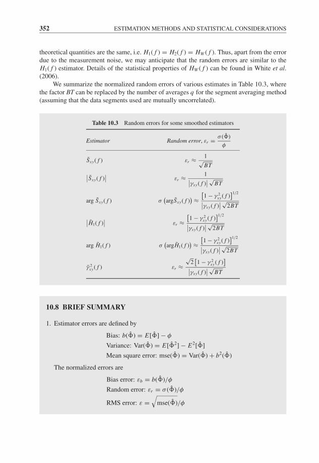
JWBK207-10 JWBK207-Shin January 18, 2008 8:20 Char Count= 0
352 ESTIMATION METHODS AND STATISTICAL CONSIDERATIONS
theoretical quantities are the same, i.e. H1( f ) = H2( f ) = HW ( f ). Thus, apart from the errordue to the measurement noise, we may anticipate that the random errors are similar to theH1( f ) estimator. Details of the statistical properties of HW ( f ) can be found in White et al.(2006).
We summarize the normalized random errors of various estimates in Table 10.3, wherethe factor BT can be replaced by the number of averages q for the segment averaging method(assuming that the data segments used are mutually uncorrelated).
Table 10.3 Random errors for some smoothed estimators
Estimator Random error, εr = σ (�)
φ
Sxy( f ) εr ≈ 1√BT∣∣Sxy( f )
∣∣ εr ≈ 1∣∣γxy( f )∣∣ √BT
arg Sxy( f ) σ(argSxy( f )
) ≈[1 − γ 2
xy( f )]1/2∣∣γxy( f )
∣∣ √2BT
∣∣H1( f )∣∣ εr ≈
[1 − γ 2
xy( f )]1/2∣∣γxy( f )
∣∣ √2BT
arg H1( f ) σ(argH1( f )
) ≈[1 − γ 2
xy( f )]1/2∣∣γxy( f )
∣∣ √2BT
γ 2xy( f ) εr ≈
√2
[1 − γ 2
xy( f )]∣∣γxy( f )
∣∣ √BT
10.8 BRIEF SUMMARY
1. Estimator errors are defined by
Bias: b(�) = E[�] − φ
Variance: Var(�) = E[�2] − E2[�]
Mean square error: mse(�) = Var(�) + b2(�)
The normalized errors are
Bias error: εb = b(�)/φ
Random error: εr = σ (�)/φ
RMS error: ε =√
mse(�)/φ
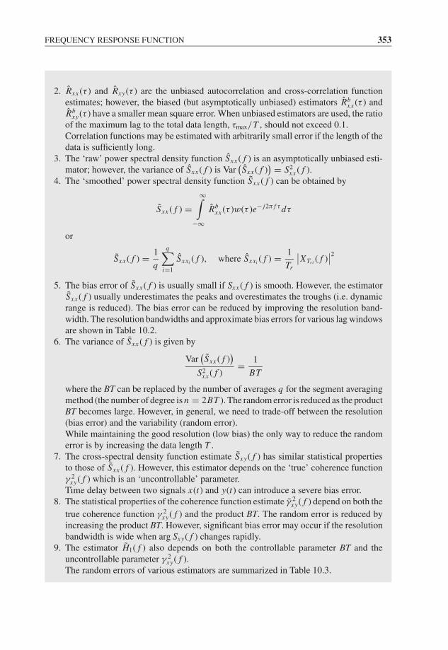
JWBK207-10 JWBK207-Shin January 18, 2008 8:20 Char Count= 0
FREQUENCY RESPONSE FUNCTION 353
2. Rxx (τ ) and Rxy(τ ) are the unbiased autocorrelation and cross-correlation functionestimates; however, the biased (but asymptotically unbiased) estimators Rb
xx (τ ) andRb
xy(τ ) have a smaller mean square error. When unbiased estimators are used, the ratioof the maximum lag to the total data length, τmax/T , should not exceed 0.1.Correlation functions may be estimated with arbitrarily small error if the length of thedata is sufficiently long.
3. The ‘raw’ power spectral density function Sxx ( f ) is an asymptotically unbiased esti-mator; however, the variance of Sxx ( f ) is Var
(Sxx ( f )
) = S2xx ( f ).
4. The ‘smoothed’ power spectral density function Sxx ( f ) can be obtained by
Sxx ( f ) =∞∫
−∞Rb
xx (τ )w(τ )e− j2π f τ dτ
or
Sxx ( f ) = 1
q
q∑i=1
Sxxi ( f ), where Sxxi ( f ) = 1
Tr
∣∣XTri ( f )∣∣2
5. The bias error of Sxx ( f ) is usually small if Sxx ( f ) is smooth. However, the estimatorSxx ( f ) usually underestimates the peaks and overestimates the troughs (i.e. dynamicrange is reduced). The bias error can be reduced by improving the resolution band-width. The resolution bandwidths and approximate bias errors for various lag windowsare shown in Table 10.2.
6. The variance of Sxx ( f ) is given by
Var(Sxx ( f )
)S2
xx ( f )= 1
BT
where the BT can be replaced by the number of averages q for the segment averagingmethod (the number of degree is n = 2BT ). The random error is reduced as the productBT becomes large. However, in general, we need to trade-off between the resolution(bias error) and the variability (random error).While maintaining the good resolution (low bias) the only way to reduce the randomerror is by increasing the data length T .
7. The cross-spectral density function estimate Sxy( f ) has similar statistical propertiesto those of Sxx ( f ). However, this estimator depends on the ‘true’ coherence functionγ 2
xy( f ) which is an ‘uncontrollable’ parameter.Time delay between two signals x(t) and y(t) can introduce a severe bias error.
8. The statistical properties of the coherence function estimate γ 2xy( f ) depend on both the
true coherence function γ 2xy( f ) and the product BT. The random error is reduced by
increasing the product BT. However, significant bias error may occur if the resolutionbandwidth is wide when arg Sxy( f ) changes rapidly.
9. The estimator H1( f ) also depends on both the controllable parameter BT and theuncontrollable parameter γ 2
xy( f ).The random errors of various estimators are summarized in Table 10.3.
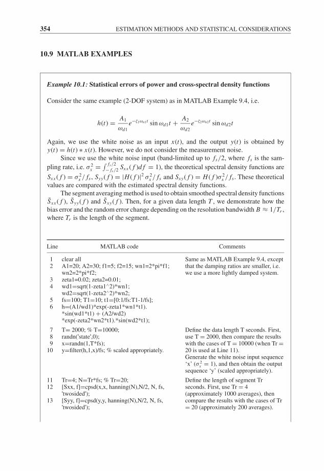
JWBK207-10 JWBK207-Shin January 18, 2008 8:20 Char Count= 0
354 ESTIMATION METHODS AND STATISTICAL CONSIDERATIONS
10.9 MATLAB EXAMPLES
Example 10.1: Statistical errors of power and cross-spectral density functions
Consider the same example (2-DOF system) as in MATLAB Example 9.4, i.e.
h(t) = A1
ωd1
e−ζ1ωn1t sin ωd1t + A2
ωd2
e−ζ2ωn2t sin ωd2t
Again, we use the white noise as an input x(t), and the output y(t) is obtained byy(t) = h(t) ∗ x(t). However, we do not consider the measurement noise.
Since we use the white noise input (band-limited up to fs/2, where fs is the sam-
pling rate, i.e. σ 2x = ∫ fs/2
− fs/2Sxx ( f )d f = 1), the theoretical spectral density functions are
Sxx ( f ) = σ 2x / fs , Syy( f ) = |H ( f )|2 σ 2
x / fs and Sxy( f ) = H ( f )σ 2x / fs . These theoretical
values are compared with the estimated spectral density functions.The segment averaging method is used to obtain smoothed spectral density functions
Sxx ( f ), S yy( f ) and Sxy( f ). Then, for a given data length T , we demonstrate how thebias error and the random error change depending on the resolution bandwidth B ≈ 1/Tr ,where Tr is the length of the segment.
Line MATLAB code Comments
12
34
56
clear allA1=20; A2=30; f1=5; f2=15; wn1=2*pi*f1;wn2=2*pi*f2;zeta1=0.02; zeta2=0.01;wd1=sqrt(1-zeta1∧2)*wn1;wd2=sqrt(1-zeta2∧2)*wn2;fs=100; T1=10; t1=[0:1/fs:T1-1/fs];h=(A1/wd1)*exp(-zeta1*wn1*t1).*sin(wd1*t1) + (A2/wd2)*exp(-zeta2*wn2*t1).*sin(wd2*t1);
Same as MATLAB Example 9.4, exceptthat the damping ratios are smaller, i.e.we use a more lightly damped system.
789
10
T= 2000; % T=10000;randn('state',0);x=randn(1,T*fs);y=filter(h,1,x)/fs; % scaled appropriately.
Define the data length T seconds. First,use T = 2000, then compare the resultswith the cases of T = 10000 (when Tr =20 is used at Line 11).Generate the white noise input sequence‘x’ (σ 2
x = 1), and then obtain the outputsequence ‘y’ (scaled appropriately).
1112
13
Tr=4; N=Tr*fs; % Tr=20;[Sxx, f]=cpsd(x,x, hanning(N),N/2, N, fs,'twosided');[Syy, f]=cpsd(y,y, hanning(N),N/2, N, fs,'twosided');
Define the length of segment Trseconds. First, use Tr = 4(approximately 1000 averages), thencompare the results with the cases of Tr= 20 (approximately 200 averages).
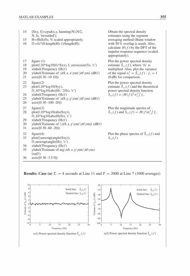
JWBK207-10 JWBK207-Shin January 18, 2008 8:20 Char Count= 0
MATLAB EXAMPLES 355
14
1516
[Sxy, f]=cpsd(x,y, hanning(N),N/2,N, fs, 'twosided');H=fft(h)/fs; % scaled appropriately.f1=fs*(0:length(H)-1)/length(H);
Obtain the spectral densityestimates using the segmentaveraging method (Hann windowwith 50 % overlap is used). Also,calculate H ( f ) by the DFT of theimpulse response sequence (scaledappropriately).
1718192021
figure (1)plot(f,10*log10(fs*Sxx), f, zeros(size(f)), 'r:')xlabel('Frequency (Hz)')ylabel('Estimate of \itS x x\rm(\itf\rm) (dB)')axis([0 30 -10 10])
Plot the power spectral densityestimate Sxx ( f ), where ‘fs’ ismultiplied. Also, plot the varianceof the signal σ 2
x = Sxx ( f ) · fs = 1(0 dB) for comparison.
2223
242526
figure(2)plot(f,10*log10(Syy),f1,10*log10(abs(H).∧2/fs), 'r:')xlabel('Frequency (Hz)')ylabel('Estimate of \itS y y\rm(\itf\rm) (dB)')axis([0 30 -100 -20])
Plot the power spectral densityestimate S yy( f ) and the theoreticalpower spectral density functionSyy( f ) = |H ( f )|2 σ 2
x
/fs .
2728
293031
figure(3)plot(f,10*log10(abs(Sxy)),f1,10*log10(abs(H)/fs), 'r:')xlabel('Frequency (Hz)')ylabel('Estimate of |\itS x y\rm(\itf\rm)| (dB)')axis([0 30 -60 -20])
Plot the magnitude spectra ofSxy( f ) and Sxy( f ) = H ( f )σ 2
x
/fs .
3233
3435
36
figure(4)plot(f,unwrap(angle(Sxy)),f1,unwrap(angle(H)), 'r:')xlabel('Frequency (Hz)')ylabel('Estimate of arg\itS x y\rm(\itf\rm)(rad)')axis([0 30 -3.5 0])
Plot the phase spectra of Sxy( f ) andSxy( f ).
Results: Case (a) Tr = 4 seconds at Line 11 and T = 2000 at Line 7 (1000 averages)
0 5 10 15 20 25 30–10
–8
–6
–4
–2
0
2
4
6
8
10
Frequency (Hz)
(a1) Power spectral density function Sxx ( f ) (a2) Power spectral density function Syy ( f )
Est
imat
e of
S xx
(f)
(dB
)
Solid line: ( )
Dashed line: ( )
xx
xx
S f
S f
0 5 10 15 20 25 30
Frequency (Hz)
Solid line: ( )
Dashed line: ( )
yy
yy
S f
S f
Est
imat
e of
S yy
(f)
(dB
)
–100
–90
–80
–70
–60
–50
–40
–30
–20
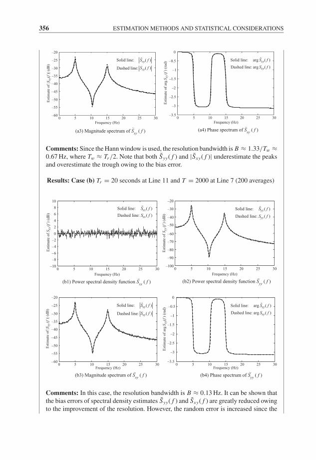
JWBK207-10 JWBK207-Shin January 18, 2008 8:20 Char Count= 0
356 ESTIMATION METHODS AND STATISTICAL CONSIDERATIONS
(a3) Magnitude spectrum of Sxy ( f )(a4) Phase spectrum of Sxy ( f )
0 5 10 15 20 25 30Frequency (Hz)
–3.5
–3
–2.5
–2
–1.5
–1
–0.5
0
Est
imat
e o
f ar
gS x
y(f
)(r
ad) Solid line: arg ( )
Dashed line: arg ( )
xy
xy
S f
S f
Solid line: ( )
( )Dashed line:
xy
xy
S f
S f
0 5 10 15 20 25 30Frequency (Hz)
Est
imat
e o
f |S
xy(f
)|(d
B)
–60
–55
–50
–45
–40
–35
–30
–25
–20
Comments: Since the Hann window is used, the resolution bandwidth is B ≈ 1.33/Tw ≈0.67 Hz, where Tw ≈ Tr/2. Note that both S yy( f ) and |Sxy( f )| underestimate the peaksand overestimate the trough owing to the bias error.
Results: Case (b) Tr = 20 seconds at Line 11 and T = 2000 at Line 7 (200 averages)
0 5 10 15 20 25 30–10
–8
–6
–4
–2
0
2
4
6
8
10
Frequency (Hz)
Est
imat
e o
f S x
x(f
)(d
B)
Solid line: ( )
Dashed line: ( )
xx
xx
S f
S f
0 5 10 15 20 25 30
Frequency (Hz)
Solid line: ( )
Dashed line: ( )
yy
yy
S f
S f
Est
imat
e o
f S y
y(f
)(d
B)
–100
–90
–80
–70
–60
–50
–40
–30
–20
(b1) Power spectral density function Sxx ( f ) (b2) Power spectral density function Syy ( f )
0 5 10 15 20 25 30Frequency (Hz)
Solid line: arg ( )
Dashed line: arg ( )
xy
xy
S f
S f
–3.5
–3
–2.5
–2
–1.5
–1
–0.5
0
Est
imat
e of
arg
S xy(
f)(r
ad)
Solid line: ( )
( )Dashed line:
xy
xy
S f
S f
0 5 10 15 20 25 30Frequency (Hz)
Est
imat
e of
|Sxy
(f)|
(dB
)
–60
–55
–50
–45
–40
–35
–30
–25
–20
(b3) Magnitude spectrum of Sxy ( f ) (b4) Phase spectrum of Syy ( f )
Comments: In this case, the resolution bandwidth is B ≈ 0.13 Hz. It can be shown thatthe bias errors of spectral density estimates S yy( f ) and Sxy( f ) are greatly reduced owingto the improvement of the resolution. However, the random error is increased since the
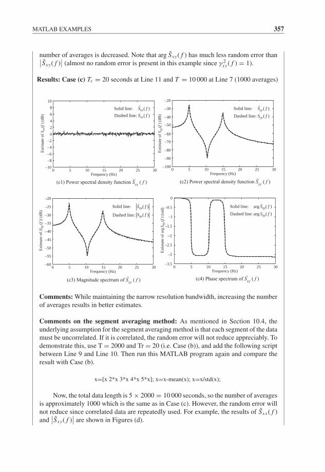
JWBK207-10 JWBK207-Shin January 18, 2008 8:20 Char Count= 0
MATLAB EXAMPLES 357
number of averages is decreased. Note that arg Sxy( f ) has much less random error than∣∣Sxy( f )∣∣ (almost no random error is present in this example since γ 2
xy( f ) = 1).
Results: Case (c) Tr = 20 seconds at Line 11 and T = 10 000 at Line 7 (1000 averages)
0 5 10 15 20 25 30–10
–8
–6
–4
–2
0
2
4
6
8
10
Frequency (Hz)
Est
imat
e of
Sxx
(f)
(dB
)
Solid line: ( )
Dashed line: ( )xx
xx
S f
S f
0 5 10 15 20 25 30Frequency (Hz)
Solid line: ( )
Dashed line: ( )yy
yy
S f
S f
Est
imat
e of
Syy
(f)
(dB
)
–100
–90
–80
–70
–60
–50
–40
–30
–20
(c1) Power spectral density function Sxx ( f ) (c2) Power spectral density function Syy ( f )
0 5 10 15 20 25 30Frequency (Hz)
Solid line: arg ( )
Dashed line: arg ( )xy
xy
S f
S f
–3.5
–3
–2.5
–2
–1.5
–1
–0.5
0
Est
imat
e of
arg
S xy
(f)
(rad
)Solid line: ( )
( )Dashed line:
xy
xy
S f
S f
0 5 10 15 20 25 30Frequency (Hz)
Est
imat
e of
|Sxy
(f)|
(dB
)
–60
–55
–50
–45
–40
–35
–30
–25
–20
(c3) Magnitude spectrum of Sxy ( f )(c4) Phase spectrum of Sxy ( f )
Comments: While maintaining the narrow resolution bandwidth, increasing the numberof averages results in better estimates.
Comments on the segment averaging method: As mentioned in Section 10.4, theunderlying assumption for the segment averaging method is that each segment of the datamust be uncorrelated. If it is correlated, the random error will not reduce appreciably. Todemonstrate this, use T = 2000 and Tr = 20 (i.e. Case (b)), and add the following scriptbetween Line 9 and Line 10. Then run this MATLAB program again and compare theresult with Case (b).
x=[x 2*x 3*x 4*x 5*x]; x=x-mean(x); x=x/std(x);
Now, the total data length is 5 × 2000 = 10 000 seconds, so the number of averagesis approximately 1000 which is the same as in Case (c). However, the random error willnot reduce since correlated data are repeatedly used. For example, the results of Sxx ( f )and
∣∣Sxy( f )∣∣ are shown in Figures (d).
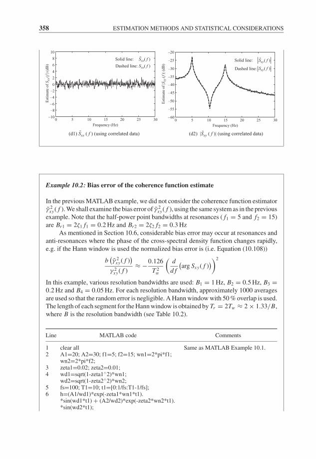
JWBK207-10 JWBK207-Shin January 18, 2008 8:20 Char Count= 0
358 ESTIMATION METHODS AND STATISTICAL CONSIDERATIONS
0 5 10 15 20 25 30–10
–8
–6
–4
–2
0
2
4
6
8
10
Frequency (Hz)
Est
imat
e o
f S x
x(f
)(d
B)
Solid line: ( )
Dashed line: ( )
xx
xx
S f
S f
(d1) Sxx ( f ) (using correlated data) (d2) |Sxy ( f )| (using correlated data)
Solid line: ( )
( )Dashed line:
xy
xy
S f
S f
0 5 10 15 20 25 30
Frequency (Hz)
Est
imat
e o
f |S
xy(f
)|(d
B)
–60
–55
–50
–45
–40
–35
–30
–25
–20
Example 10.2: Bias error of the coherence function estimate
In the previous MATLAB example, we did not consider the coherence function estimatorγ 2
xy( f ). We shall examine the bias error of γ 2xy( f ), using the same system as in the previous
example. Note that the half-power point bandwidths at resonances ( f1 = 5 and f2 = 15)are Br1 = 2ζ1 f1 = 0.2 Hz and Br2 = 2ζ2 f2 = 0.3 Hz
As mentioned in Section 10.6, considerable bias error may occur at resonances andanti-resonances where the phase of the cross-spectral density function changes rapidly,e.g. if the Hann window is used the normalized bias error is (i.e. Equation (10.108))
b(γ 2
xy( f ))
γ 2xy( f )
≈ −0.126
T 2w
(d
d f
(arg Sxy( f )
))2
In this example, various resolution bandwidths are used: B1 = 1 Hz, B2 = 0.5 Hz, B3 =0.2 Hz and B4 = 0.05 Hz. For each resolution bandwidth, approximately 1000 averagesare used so that the random error is negligible. A Hann window with 50 % overlap is used.The length of each segment for the Hann window is obtained by Tr = 2Tw ≈ 2 × 1.33/B,where B is the resolution bandwidth (see Table 10.2).
Line MATLAB code Comments
12
34
56
clear allA1=20; A2=30; f1=5; f2=15; wn1=2*pi*f1;wn2=2*pi*f2;zeta1=0.02; zeta2=0.01;wd1=sqrt(1-zeta1∧2)*wn1;wd2=sqrt(1-zeta2∧2)*wn2;fs=100; T1=10; t1=[0:1/fs:T1-1/fs];h=(A1/wd1)*exp(-zeta1*wn1*t1).*sin(wd1*t1) + (A2/wd2)*exp(-zeta2*wn2*t1).*sin(wd2*t1);
Same as MATLAB Example 10.1.
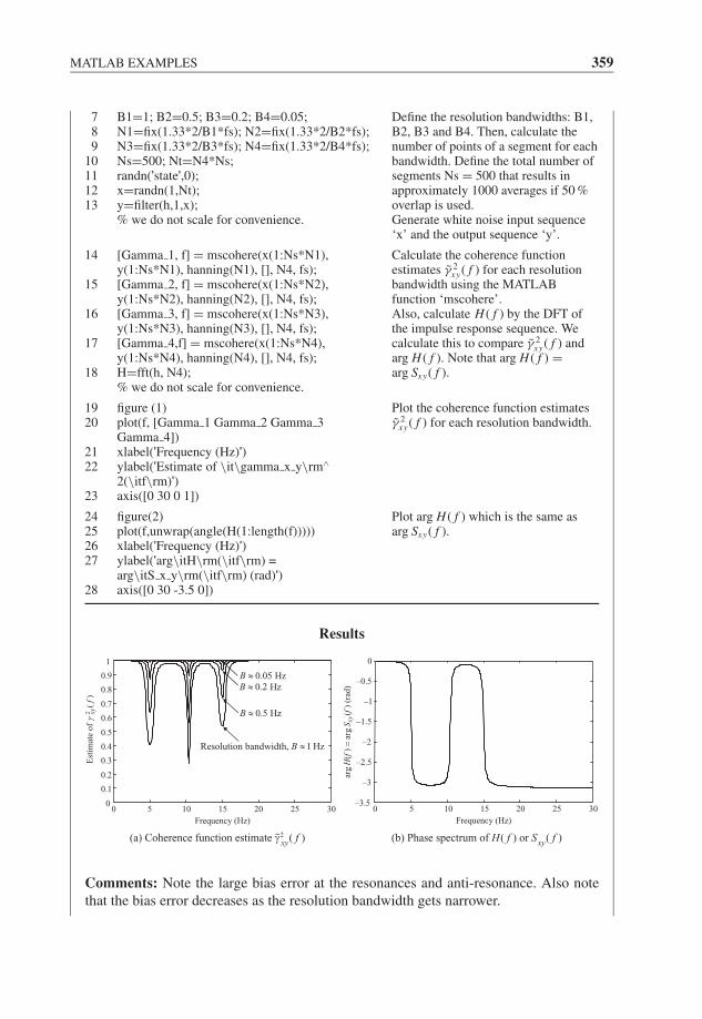
JWBK207-10 JWBK207-Shin January 18, 2008 8:20 Char Count= 0
MATLAB EXAMPLES 359
789
10111213
B1=1; B2=0.5; B3=0.2; B4=0.05;N1=fix(1.33*2/B1*fs); N2=fix(1.33*2/B2*fs);N3=fix(1.33*2/B3*fs); N4=fix(1.33*2/B4*fs);Ns=500; Nt=N4*Ns;randn('state',0);x=randn(1,Nt);y=filter(h,1,x);% we do not scale for convenience.
Define the resolution bandwidths: B1,B2, B3 and B4. Then, calculate thenumber of points of a segment for eachbandwidth. Define the total number ofsegments Ns = 500 that results inapproximately 1000 averages if 50 %overlap is used.Generate white noise input sequence‘x’ and the output sequence ‘y’.
14
15
16
17
18
[Gamma 1, f] = mscohere(x(1:Ns*N1),y(1:Ns*N1), hanning(N1), [], N4, fs);[Gamma 2, f] = mscohere(x(1:Ns*N2),y(1:Ns*N2), hanning(N2), [], N4, fs);[Gamma 3, f] = mscohere(x(1:Ns*N3),y(1:Ns*N3), hanning(N3), [], N4, fs);[Gamma 4,f] = mscohere(x(1:Ns*N4),y(1:Ns*N4), hanning(N4), [], N4, fs);H=fft(h, N4);% we do not scale for convenience.
Calculate the coherence functionestimates γ 2
xy( f ) for each resolutionbandwidth using the MATLABfunction ‘mscohere’.Also, calculate H ( f ) by the DFT ofthe impulse response sequence. Wecalculate this to compare γ 2
xy( f ) andarg H ( f ). Note that arg H ( f ) =arg Sxy( f ).
1920
2122
23
figure (1)plot(f, [Gamma 1 Gamma 2 Gamma 3Gamma 4])xlabel('Frequency (Hz)')ylabel('Estimate of \it\gamma x y\rm∧
2(\itf\rm)')axis([0 30 0 1])
Plot the coherence function estimatesγ 2
xy( f ) for each resolution bandwidth.
24252627
28
figure(2)plot(f,unwrap(angle(H(1:length(f)))))xlabel('Frequency (Hz)')ylabel('arg\itH\rm(\itf\rm) =arg\itS x y\rm(\itf\rm) (rad)')axis([0 30 -3.5 0])
Plot arg H ( f ) which is the same asarg Sxy( f ).
Results
0 5 10 15 20 25 300
0.1
0.2
0.3
0.4
0.5
0.6
0.7
0.8
0.9
1
Frequency (Hz)
(a) Coherence function estimate γ2xy( f ) (b) Phase spectrum of H( f ) or Sxy( f )
Est
imat
e of
γ2 xy
(f)
Resolution bandwidth, 1 HzB ≈
0.2 HzB ≈
0.5 HzB ≈
0.05 HzB ≈
0 5 10 15 20 25 30–3.5
–3
–2.5
–2
–1.5
–1
–0.5
0
Frequency (Hz)
arg
H(f
)=
arg
S xy(
f) (
rad)
∼
Comments: Note the large bias error at the resonances and anti-resonance. Also notethat the bias error decreases as the resolution bandwidth gets narrower.
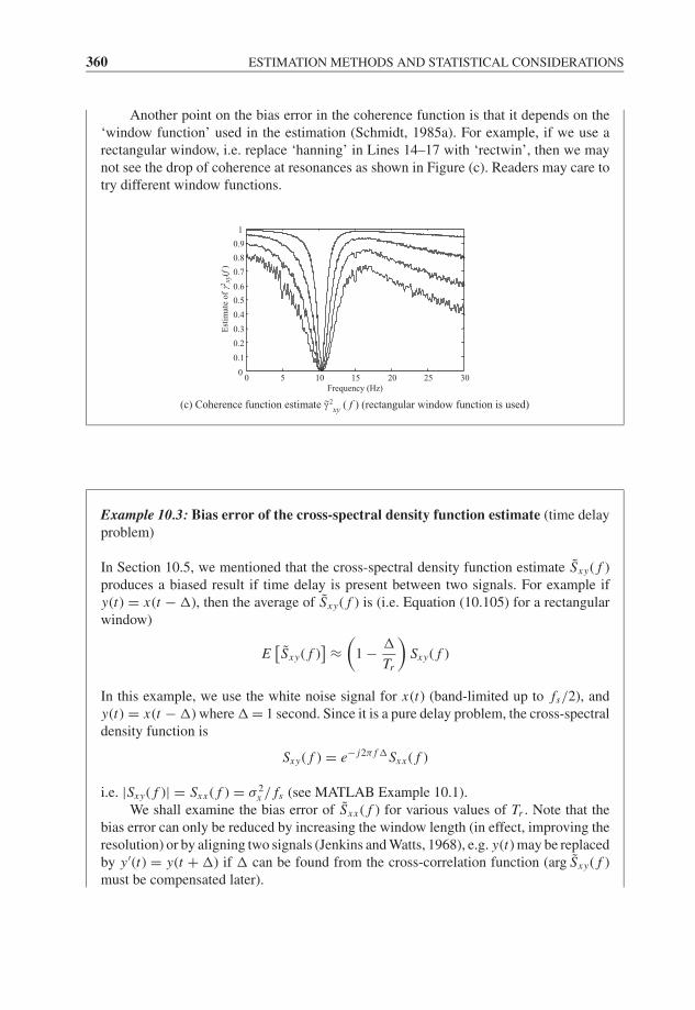
JWBK207-10 JWBK207-Shin January 18, 2008 8:20 Char Count= 0
360 ESTIMATION METHODS AND STATISTICAL CONSIDERATIONS
Another point on the bias error in the coherence function is that it depends on the‘window function’ used in the estimation (Schmidt, 1985a). For example, if we use arectangular window, i.e. replace ‘hanning’ in Lines 14–17 with ‘rectwin’, then we maynot see the drop of coherence at resonances as shown in Figure (c). Readers may care totry different window functions.
0 5 10 15 20 25 30Frequency (Hz)
0
0.1
0.2
0.3
0.4
0.5
0.6
0.7
0.8
0.9
1E
stim
ate
of
γ2xy
(f)
(c) Coherence function estimate γ2xy ( f ) (rectangular window function is used)∼
Example 10.3: Bias error of the cross-spectral density function estimate (time delayproblem)
In Section 10.5, we mentioned that the cross-spectral density function estimate Sxy( f )produces a biased result if time delay is present between two signals. For example ify(t) = x(t − ), then the average of Sxy( f ) is (i.e. Equation (10.105) for a rectangularwindow)
E[Sxy( f )
] ≈(
1 −
Tr
)Sxy( f )
In this example, we use the white noise signal for x(t) (band-limited up to fs/2), andy(t) = x(t − ) where = 1 second. Since it is a pure delay problem, the cross-spectraldensity function is
Sxy( f ) = e− j2π f Sxx ( f )
i.e. |Sxy( f )| = Sxx ( f ) = σ 2x / fs (see MATLAB Example 10.1).
We shall examine the bias error of Sxx ( f ) for various values of Tr . Note that thebias error can only be reduced by increasing the window length (in effect, improving theresolution) or by aligning two signals (Jenkins and Watts, 1968), e.g. y(t) may be replacedby y′(t) = y(t + ) if can be found from the cross-correlation function (arg Sxy( f )must be compensated later).
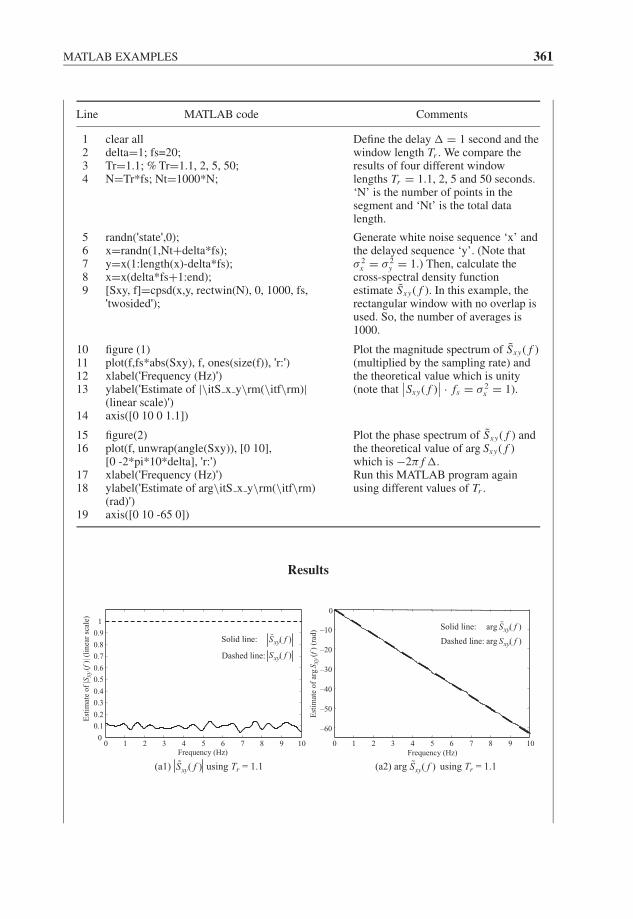
JWBK207-10 JWBK207-Shin January 18, 2008 8:20 Char Count= 0
MATLAB EXAMPLES 361
Line MATLAB code Comments
1234
clear alldelta=1; fs=20;Tr=1.1; % Tr=1.1, 2, 5, 50;N=Tr*fs; Nt=1000*N;
Define the delay = 1 second and thewindow length Tr . We compare theresults of four different windowlengths Tr = 1.1, 2, 5 and 50 seconds.‘N’ is the number of points in thesegment and ‘Nt’ is the total datalength.
56789
randn('state',0);x=randn(1,Nt+delta*fs);y=x(1:length(x)-delta*fs);x=x(delta*fs+1:end);[Sxy, f]=cpsd(x,y, rectwin(N), 0, 1000, fs,'twosided');
Generate white noise sequence ‘x’ andthe delayed sequence ‘y’. (Note thatσ 2
x = σ 2y = 1.) Then, calculate the
cross-spectral density functionestimate Sxy( f ). In this example, therectangular window with no overlap isused. So, the number of averages is1000.
10111213
14
figure (1)plot(f,fs*abs(Sxy), f, ones(size(f)), 'r:')xlabel('Frequency (Hz)')ylabel('Estimate of |\itS x y\rm(\itf\rm)|(linear scale)')axis([0 10 0 1.1])
Plot the magnitude spectrum of Sxy( f )(multiplied by the sampling rate) andthe theoretical value which is unity(note that
∣∣Sxy( f )∣∣ · fs = σ 2
x = 1).
1516
1718
19
figure(2)plot(f, unwrap(angle(Sxy)), [0 10],[0 -2*pi*10*delta], 'r:')xlabel('Frequency (Hz)')ylabel('Estimate of arg\itS x y\rm(\itf\rm)(rad)')axis([0 10 -65 0])
Plot the phase spectrum of Sxy( f ) andthe theoretical value of arg Sxy( f )which is −2π f .Run this MATLAB program againusing different values of Tr .
Results
0 1 2 3 4 5 6 7 8 9 10Frequency (Hz)
0
0.1
0.2
0.3
0.4
0.5
0.6
0.7
0.8
0.9
1
Est
imat
e of
|Sxy
(f)|
(lin
ear
scal
e)
Solid line: ( )
( )Dashed line:
xy
xy
S f
S f
(a1) using Tr = 1.1( )xyS f (a2) arg using Tr = 1.1( )xyS f
Solid line: arg ( )
Dashed line: arg ( )
xy
xy
S f
S f
0 1 2 3 4 5 6 7 8 9 10
Est
imat
e o
f ar
gS x
y(f
)(r
ad)
–60
–50
–40
–30
–20
–10
0
Frequency (Hz)
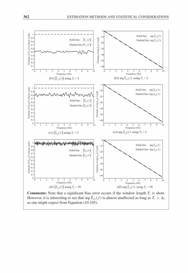
JWBK207-10 JWBK207-Shin January 18, 2008 8:20 Char Count= 0
362 ESTIMATION METHODS AND STATISTICAL CONSIDERATIONS
(b2) arg using Tr = 2( )xyS f(b1) using Tr = 2( )xyS f
0 1 2 3 4 5 6 7 8 9 10Frequency (Hz)
Solid line: ( )
( )Dashed line:
xy
xy
S f
S f
0
0.1
0.2
0.3
0.4
0.5
0.6
0.7
0.8
0.9
1
Est
imat
e of
|Sxy
(f)|
(lin
ear
scal
e)
Solid line: arg ( )
Dashed line: arg ( )
xy
xy
S f
S f
0 1 2 3 4 5 6 7 8 9 10Frequency (Hz)
Est
imat
e of
arg
S xy(
f)(r
ad)
– 60
–50
– 40
–30
–20
–10
0
(c2) arg using Tr = 5( )xyS f(c1) using Tr = 5( )xyS f
0 1 2 3 4 5 6 7 8 9 10Frequency (Hz)
Solid line: ( )
( )Dashed line:
xy
xy
S f
S f
0
0.1
0.2
0.3
0.4
0.5
0.6
0.7
0.8
0.9
1
Est
imat
e of
|Sxy
(f)|
(lin
ear
scal
e)
Solid line: arg ( )
Dashed line: arg ( )
xy
xy
S f
S f
0 1 2 3 4 5 6 7 8 9 10Frequency (Hz)
Est
imat
e of
arg
S xy(
f)(r
ad)
–60
–50
–40
–30
–20
–10
0
0 1 2 3 4 5 6 7 8 9 10Frequency (Hz)
Solid line: ( )
( )Dashed line:
xy
xy
S f
S f
0
0.1
0.2
0.3
0.4
0.5
0.6
0.7
0.8
0.9
1
Est
imat
e of
|Sxy
(f)|
(lin
ear
scal
e)
Solid line: arg ( )
Dashed line: arg ( )
xy
xy
S f
S f
0 1 2 3 4 5 6 7 8 9 10Frequency (Hz)
Est
imat
e of
arg
S xy
(f)
(rad
)
–60
–50
–40
–30
–20
–10
0
(d1) using Tr = 50( )xyS f (d2) arg using Tr = 50( )xyS f
Comments: Note that a significant bias error occurs if the window length Tr is short.However, it is interesting to see that arg Sxy( f ) is almost unaffected as long as Tr > ,as one might expect from Equation (10.105).
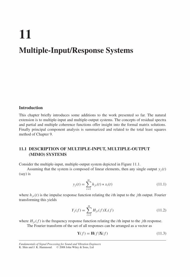
JWBK207-11 JWBK207-Shin January 18, 2008 8:21 Char Count= 0
11Multiple-Input/Response Systems
Introduction
This chapter briefly introduces some additions to the work presented so far. The naturalextension is to multiple-input and multiple-output systems. The concepts of residual spectraand partial and multiple coherence functions offer insight into the formal matrix solutions.Finally principal component analysis is summarized and related to the total least squaresmethod of Chapter 9.
11.1 DESCRIPTION OF MULTIPLE-INPUT, MULTIPLE-OUTPUT(MIMO) SYSTEMS
Consider the multiple-input, multiple-output system depicted in Figure 11.1.Assuming that the system is composed of linear elements, then any single output y j (t)
(say) is
y j (t) =m∑
i=1
h ji (t) ∗ xi (t) (11.1)
where h ji (t) is the impulse response function relating the i th input to the j th output. Fouriertransforming this yields
Y j ( f ) =m∑
i=1
Hji ( f )Xi ( f ) (11.2)
where Hji ( f ) is the frequency response function relating the i th input to the j th response.The Fourier transform of the set of all responses can be arranged as a vector as
Y( f ) = H( f )X( f ) (11.3)
Fundamentals of Signal Processing for Sound and Vibration EngineersK. Shin and J. K. Hammond. C© 2008 John Wiley & Sons, Ltd
363
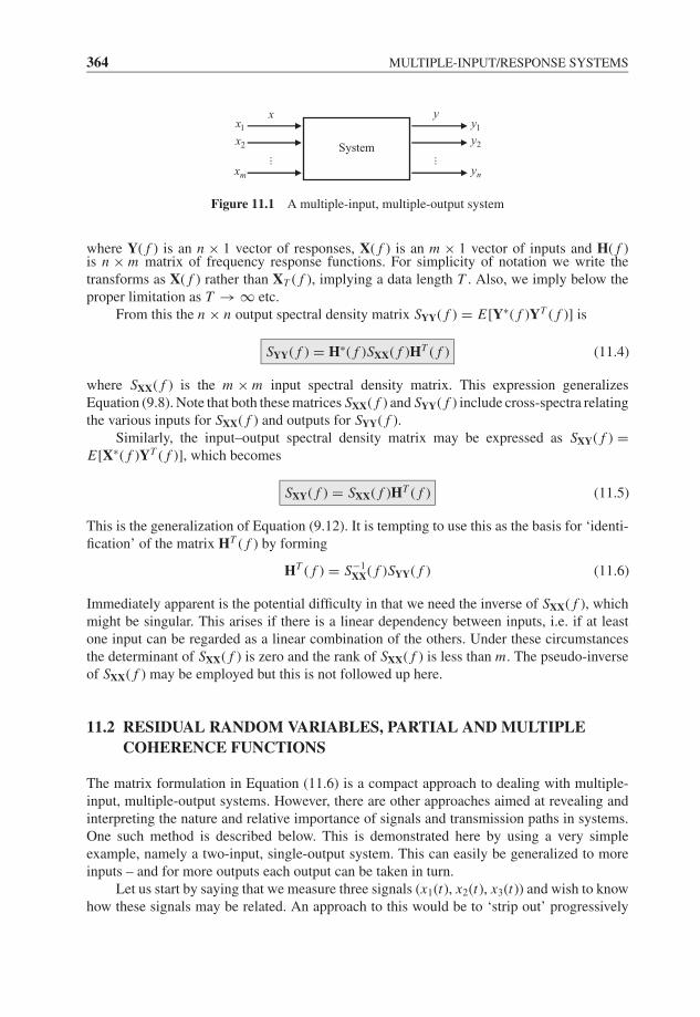
JWBK207-11 JWBK207-Shin January 18, 2008 8:21 Char Count= 0
364 MULTIPLE-INPUT/RESPONSE SYSTEMS
x
System
1yy
1x
2y2x
nymx
Figure 11.1 A multiple-input, multiple-output system
where Y( f ) is an n × 1 vector of responses, X( f ) is an m × 1 vector of inputs and H( f )is n × m matrix of frequency response functions. For simplicity of notation we write thetransforms as X( f ) rather than XT ( f ), implying a data length T . Also, we imply below theproper limitation as T → ∞ etc.
From this the n × n output spectral density matrix SYY( f ) = E[Y∗( f )YT ( f )] is
SYY( f ) = H∗( f )SXX( f )HT ( f ) (11.4)
where SXX( f ) is the m × m input spectral density matrix. This expression generalizesEquation (9.8). Note that both these matrices SXX( f ) and SYY( f ) include cross-spectra relatingthe various inputs for SXX( f ) and outputs for SYY( f ).
Similarly, the input–output spectral density matrix may be expressed as SXY( f ) =E[X∗( f )YT ( f )], which becomes
SXY( f ) = SXX( f )HT ( f ) (11.5)
This is the generalization of Equation (9.12). It is tempting to use this as the basis for ‘identi-fication’ of the matrix HT ( f ) by forming
HT ( f ) = S−1XX( f )SYY( f ) (11.6)
Immediately apparent is the potential difficulty in that we need the inverse of SXX( f ), whichmight be singular. This arises if there is a linear dependency between inputs, i.e. if at leastone input can be regarded as a linear combination of the others. Under these circumstancesthe determinant of SXX( f ) is zero and the rank of SXX( f ) is less than m. The pseudo-inverseof SXX( f ) may be employed but this is not followed up here.
11.2 RESIDUAL RANDOM VARIABLES, PARTIAL AND MULTIPLECOHERENCE FUNCTIONS
The matrix formulation in Equation (11.6) is a compact approach to dealing with multiple-input, multiple-output systems. However, there are other approaches aimed at revealing andinterpreting the nature and relative importance of signals and transmission paths in systems.One such method is described below. This is demonstrated here by using a very simpleexample, namely a two-input, single-output system. This can easily be generalized to moreinputs – and for more outputs each output can be taken in turn.
Let us start by saying that we measure three signals (x1(t), x2(t), x3(t)) and wish to knowhow these signals may be related. An approach to this would be to ‘strip out’ progressively
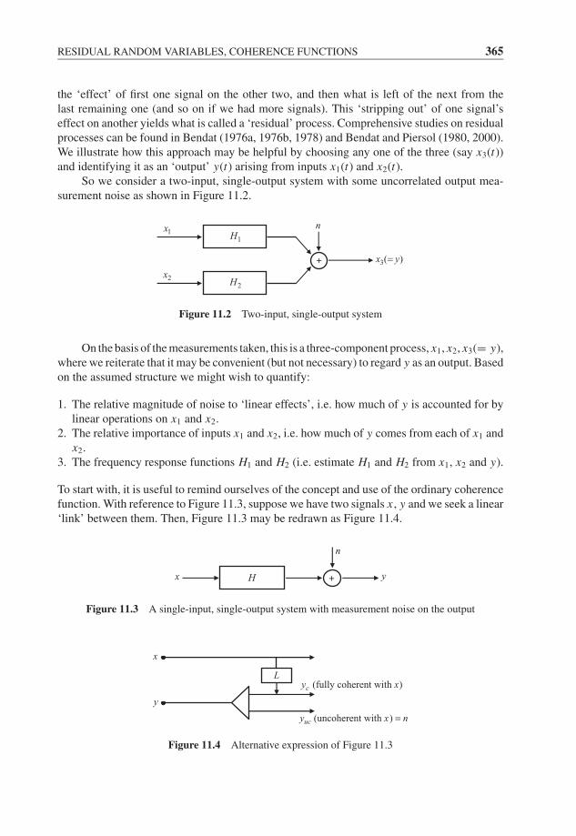
JWBK207-11 JWBK207-Shin January 18, 2008 8:21 Char Count= 0
RESIDUAL RANDOM VARIABLES, COHERENCE FUNCTIONS 365
the ‘effect’ of first one signal on the other two, and then what is left of the next from thelast remaining one (and so on if we had more signals). This ‘stripping out’ of one signal’seffect on another yields what is called a ‘residual’ process. Comprehensive studies on residualprocesses can be found in Bendat (1976a, 1976b, 1978) and Bendat and Piersol (1980, 2000).We illustrate how this approach may be helpful by choosing any one of the three (say x3(t))and identifying it as an ‘output’ y(t) arising from inputs x1(t) and x2(t).
So we consider a two-input, single-output system with some uncorrelated output mea-surement noise as shown in Figure 11.2.
1x
+
n
3( )x y=
1H
2x2H
Figure 11.2 Two-input, single-output system
On the basis of the measurements taken, this is a three-component process, x1, x2, x3(= y),where we reiterate that it may be convenient (but not necessary) to regard y as an output. Basedon the assumed structure we might wish to quantify:
1. The relative magnitude of noise to ‘linear effects’, i.e. how much of y is accounted for bylinear operations on x1 and x2.
2. The relative importance of inputs x1 and x2, i.e. how much of y comes from each of x1 andx2.
3. The frequency response functions H1 and H2 (i.e. estimate H1 and H2 from x1, x2 and y).
To start with, it is useful to remind ourselves of the concept and use of the ordinary coherencefunction. With reference to Figure 11.3, suppose we have two signals x , y and we seek a linear‘link’ between them. Then, Figure 11.3 may be redrawn as Figure 11.4.
x +
n
yH
Figure 11.3 A single-input, single-output system with measurement noise on the output
L
x
y
(fully coherent with x )cy
(uncoherent with x )ucy n=
Figure 11.4 Alternative expression of Figure 11.3
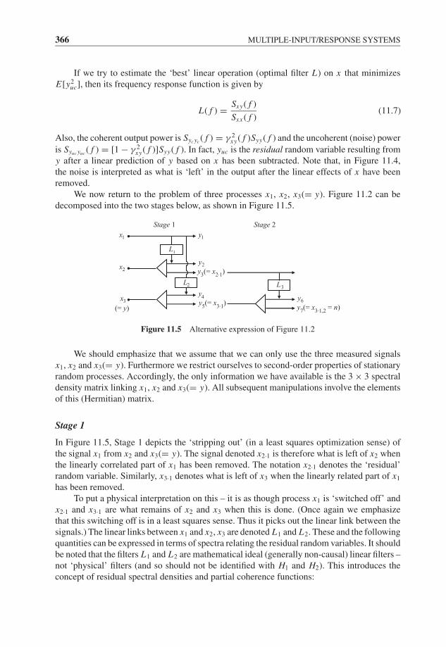
JWBK207-11 JWBK207-Shin January 18, 2008 8:21 Char Count= 0
366 MULTIPLE-INPUT/RESPONSE SYSTEMS
If we try to estimate the ‘best’ linear operation (optimal filter L) on x that minimizesE[y2
uc], then its frequency response function is given by
L( f ) = Sxy( f )
Sxx ( f )(11.7)
Also, the coherent output power is Syc yc ( f ) = γ 2xy( f )Syy( f ) and the uncoherent (noise) power
is Syuc yuc ( f ) = [1 − γ 2xy( f )]Syy( f ). In fact, yuc is the residual random variable resulting from
y after a linear prediction of y based on x has been subtracted. Note that, in Figure 11.4,the noise is interpreted as what is ‘left’ in the output after the linear effects of x have beenremoved.
We now return to the problem of three processes x1, x2, x3(= y). Figure 11.2 can bedecomposed into the two stages below, as shown in Figure 11.5.
1x
Stage 1
2y
1L
y3(= x
2.1)
y5(= x
3.1)
y7(= x
3.1,2 = n)
2x
4y
3
(= y)
x
1y
6y
Stage 2
2L3L
Figure 11.5 Alternative expression of Figure 11.2
We should emphasize that we assume that we can only use the three measured signalsx1, x2 and x3(= y). Furthermore we restrict ourselves to second-order properties of stationaryrandom processes. Accordingly, the only information we have available is the 3 × 3 spectraldensity matrix linking x1, x2 and x3(= y). All subsequent manipulations involve the elementsof this (Hermitian) matrix.
Stage 1
In Figure 11.5, Stage 1 depicts the ‘stripping out’ (in a least squares optimization sense) ofthe signal x1 from x2 and x3(= y). The signal denoted x2·1 is therefore what is left of x2 whenthe linearly correlated part of x1 has been removed. The notation x2·1 denotes the ‘residual’random variable. Similarly, x3·1 denotes what is left of x3 when the linearly related part of x1
has been removed.To put a physical interpretation on this – it is as though process x1 is ‘switched off’ and
x2·1 and x3·1 are what remains of x2 and x3 when this is done. (Once again we emphasizethat this switching off is in a least squares sense. Thus it picks out the linear link between thesignals.) The linear links between x1 and x2, x3 are denoted L1 and L2. These and the followingquantities can be expressed in terms of spectra relating the residual random variables. It shouldbe noted that the filters L1 and L2 are mathematical ideal (generally non-causal) linear filters –not ‘physical’ filters (and so should not be identified with H1 and H2). This introduces theconcept of residual spectral densities and partial coherence functions:
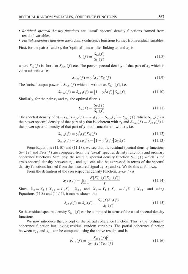
JWBK207-11 JWBK207-Shin January 18, 2008 8:21 Char Count= 0
RESIDUAL RANDOM VARIABLES, COHERENCE FUNCTIONS 367
� Residual spectral density functions are ‘usual’ spectral density functions formed fromresidual variables.� Partial coherence functions are ordinary coherence functions formed from residual variables.
First, for the pair x1 and x2, the ‘optimal’ linear filter linking x1 and x2 is
L1( f ) = S12( f )
S11( f )(11.8)
where S12( f ) is short for Sx1x2( f ) etc. The power spectral density of that part of x2 which is
coherent with x1 is
Sy2 y2( f ) = γ 2
12( f )S22( f ) (11.9)
The ‘noise’ output power is Sy3 y3( f ) which is written as S22·1( f ), i.e.
Sy3 y3( f ) = S22·1( f ) = [
1 − γ 212( f )
]S22( f ) (11.10)
Similarly, for the pair x1 and x3, the optimal filter is
L2( f ) = S13( f )
S11( f )(11.11)
The spectral density of y(= x3) is Syy( f ) = S33( f ) = Sy4 y4( f ) + Sy5 y5
( f ), where Sy4 y4( f ) is
the power spectral density of that part of y that is coherent with x1 and Sy5 y5( f ) = S33·1( f ) is
the power spectral density of that part of y that is uncoherent with x1, i.e.
Sy4 y4( f ) = γ 2
13( f )S33( f ) (11.12)
Sy5 y5( f ) = S33·1( f ) = [
1 − γ 213( f )
]S33( f ) (11.13)
From Equations (11.10) and (11.13), we see that the residual spectral density functionsS22·1( f ) and S33·1( f ) are computed from the ‘usual’ spectral density functions and ordinarycoherence functions. Similarly, the residual spectral density function S23·1( f ) which is thecross-spectral density between x2·1 and x3·1 can also be expressed in terms of the spectraldensity functions formed from the measured signal x1, x2 and x3. We do this as follows.
From the definition of the cross-spectral density function, S23·1( f ) is
S23·1( f ) = limT →∞
E[X∗2·1( f )X3·1( f )]
T(11.14)
Since X2 = Y2 + X2·1 = L1 X1 + X2·1 and X3 = Y4 + X3·1 = L2 X1 + X3·1, and usingEquations (11.8) and (11.11), it can be shown that
S23·1( f ) = S23( f ) − S21( f )S13( f )
S11( f )(11.15)
So the residual spectral density S23·1( f ) can be computed in terms of the usual spectral densityfunctions.
We now introduce the concept of the partial coherence function. This is the ‘ordinary’coherence function but linking residual random variables. The partial coherence functionbetween x2·1 and x3·1 can be computed using the above results, and is
γ 223·1( f ) = |S23·1( f )|2
S22·1( f )S33·1( f )(11.16)
JWBK207-11 JWBK207-Shin January 18, 2008 8:21 Char Count= 0
368 MULTIPLE-INPUT/RESPONSE SYSTEMS
Stage 2
In Figure 11.5, Stage 2 depicts the ‘removal’ of x2·1 from x3·1. As before, for the pair x2·1 andx3·1, the optimal filter is
L3( f ) = S23·1( f )
S22·1( f )(11.17)
In the figure, x3·1,2 denotes the residual variable arising when the linear effects of both x1 andx2 are removed from x3. The output powers of uncoherent and coherent components with x2·1are
Sy7 y7( f ) = Snn( f ) = S33·1,2( f ) = [
1 − γ 223·1( f )
]S33·1( f ) (11.18)
Sy6 y6( f ) = γ 2
23·1( f )S33·1( f ) (11.19)
Note that S33·1,2( f ) is the power spectral density of that part of y unaccounted for by linearoperations on x1 and x2, i.e. the uncorrelated noise power. Now, combining the above resultsand using Figure 11.5, the power spectral density of y can be decomposed into
Syy( f ) = S33( f ) = Sy4 y4( f ) + Sy6 y6
( f ) + Sy7 y7( f )
= γ 213( f )S33( f ) part fully coherent with x1
+ γ 223·1( f )S33·1( f ) part fully coherent with x2
after x1 has been removed from x2 and x3
+ [1 − γ 2
23·1( f )]
S33·1( f ) uncoherent with both x1 and x2 (11.20)
This equation shows the role of the partial coherence function.Note that by following the signal flow in Figure 11.5, one can easily verify that
H1( f ) = L2( f ) − L1( f )L3( f ) (11.21)
and
H2( f ) = L3( f ) (11.22)
A multiple coherence function is defined in a manner similar to that of the ordinarycoherence function. Recall that the ordinary coherence function for the system shown inFigure 11.3 can be written as γ 2
xy( f ) = (Syy( f ) − Snn( f ))/Syy( f ). Similarly, the multiple
coherence function denoted γ 2y:x ( f ) is defined as
γ 2y:x ( f ) = Syy( f ) − Snn( f )
Syy( f )(11.23)
That is the multiple coherence function γ 2y:x ( f ) is the fraction of output power accounted for
via linear operations on the inputs; it is a measure of how well the inputs account for themeasured response of the system. For the example shown above, it can be written as
γ 2y:x ( f ) = S33( f ) − S33·1,2( f )
S33( f )(11.24)
Note that the nearer γ 2y:x ( f ) is to unity, the more ‘completely’ does the linear model apply
to the three components. Using Equations (11.12) and (11.18), the above equation can be
JWBK207-11 JWBK207-Shin January 18, 2008 8:21 Char Count= 0
RESIDUAL RANDOM VARIABLES, COHERENCE FUNCTIONS 369
written as
γ 2y:x ( f ) = 1 − (
1 − γ 213( f )
) (1 − γ 2
23·1( f ))
(11.25)
which shows that it can be computed in terms of partial and ordinary coherence functions. SeeSutton et al. (1994) for applications of the multiple coherence function.
Computation of Residual Spectra and Interpretation in Termsof Gaussian Elimination
The above example illustrates the methodology. A more general computational formulationis given below which operates on the elements of the spectral density matrix of the measuredsignals. The residual spectral density function S23·1( f ) given in Equation (11.15) can begeneralized as
Si j ·k( f ) = Si j ( f ) − Sik( f )Skj ( f )
Skk( f )(11.26)
This can be extended as
Si j ·k,l( f ) = Si j ·k( f ) − Sil·k( f )Sl j ·k( f )
Sll·k( f )(11.27)
We use the above expressions to ‘condense’ successive cross-spectral density matrices, e.g.⎡⎢⎣ S11( f ) S12( f ) S13( f )
S21( f ) S22( f ) S23( f )
S31( f ) S32( f ) S33( f )
⎤⎥⎦ ⇒[
S22·1( f ) S23·1( f )
S32·1( f ) S33·1( f )
]⇒ [
S33·1,2( f )]
(11.28)
This can be extended to larger systems. This ‘condensation’ can be interpreted through Gaus-sian elimination (row manipulations) as follows (where ri is the i th row):
Step 1: r2 → r2 − r1 ×(
S21( f )
S11( f )
); r3 → r3 − r1 ×
(S31( f )
S11( f )
)gives
⎡⎢⎣ S11( f ) S12( f ) S13( f )
S21( f ) S22( f ) S23( f )
S31( f ) S32( f ) S33( f )
⎤⎥⎦ ⇒
⎡⎢⎣ S11( f ) S12( f ) S13( f )
0 S22·1( f ) S23·1( f )
0 S32·1( f ) S33·1( f )
⎤⎥⎦ (11.29)
Step 2: r3 → r3 − r2 ×(
S32·1( f )
S22·1( f )
)gives
⎡⎢⎣ S11( f ) S12( f ) S13( f )
0 S22·1( f ) S23·1( f )
0 S32·1( f ) S33·1( f )
⎤⎥⎦ ⇒
⎡⎢⎣ S11( f ) S12( f ) S13( f )
0 S22·1( f ) S23·1( f )
0 0 S33·1,2( f )
⎤⎥⎦ (11.30)
i.e. the residual spectral density functions arise naturally.
JWBK207-11 JWBK207-Shin January 18, 2008 8:21 Char Count= 0
370 MULTIPLE-INPUT/RESPONSE SYSTEMS
Further interpretation can be obtained by starting from Figure 11.2 again. Since X3( f ) =H1( f )X1( f ) + H2( f )X2( f ) + N ( f ), the cross-spectral density functions are written as
S13( f ) = H1( f )S11( f ) + H2( f )S12( f )
S23( f ) = H1( f )S21( f ) + H2( f )S22( f ) (11.31)
Solving for H1( f ) and H2( f ) using Gaussian elimination (eliminate the term H1( f )S21( f ) inthe second Equation of (11.31)) gives
S11( f )H1( f ) + S12( f )H2( f ) = S13( f )(S22( f ) − S21( f )S12( f )
S11( f )
)H2( f ) = S23( f ) − S21( f )S13( f )
S11( f )(11.32)
Thus,
H2( f ) = S23·1( f )
S22·1( f )and H1( f ) = S13( f )
S11( f )− S12( f )
S11( f )
S23·1( f )
S22·1( f )
11.3 PRINCIPAL COMPONENT ANALYSIS
Although residual spectral analysis is useful in source identification, condition monitoring,etc., the shortcoming of the method is that prior ranking of the input signals is often required(see Bendat and Piersol, 1980), i.e. a priori knowledge. Principal component analysis (PCA)is a general approach to explore correlation patterns (Otte et al., 1988).
Suppose we have three processes x1, x2, x3. Then we start as before by forming thecross-spectral density matrix
S =
⎡⎢⎣ S11( f ) S12( f ) S13( f )
S21( f ) S22( f ) S23( f )
S31( f ) S32( f ) S33( f )
⎤⎥⎦ (11.33)
Note that this is a Hermitian matrix, i.e. S = S*T = SH , where SH is the conjugate transpose.If there is a linear relationship between the processes xi , then the determinant of this matrixis zero (i.e. its rank is less than three). If there is no linear relationship then its rank is three.
Suppose the matrix is full rank (i.e. rank 3). Then eigenvalue (or singular value) decom-position gives
S = UΛUH (11.34)
where Λ is a diagonal matrix that contains eigenvalues of S, and U is a unitary matrix whosecolumns are the corresponding eigenvectors. We may describe the physical interpretation ofthis as follows. Suppose there exist three (fictitious) processes z1, z2, z3 that are mutuallyuncorrelated and from which x1, x2, x3 can be derived, i.e. for each frequency f ,⎡⎢⎣ X1( f )
X2( f )
X3( f )
⎤⎥⎦ =
⎡⎢⎣ m11( f ) m12( f ) m13( f )
m21( f ) m22( f ) m23( f )
m31( f ) m32( f ) m33( f )
⎤⎥⎦⎡⎢⎣ Z1( f )
Z2( f )
Z3( f )
⎤⎥⎦ (11.35)
i.e. X( f ) = M( f )Z( f ). Conceptually, this can be depicted as in Figure 11.6.
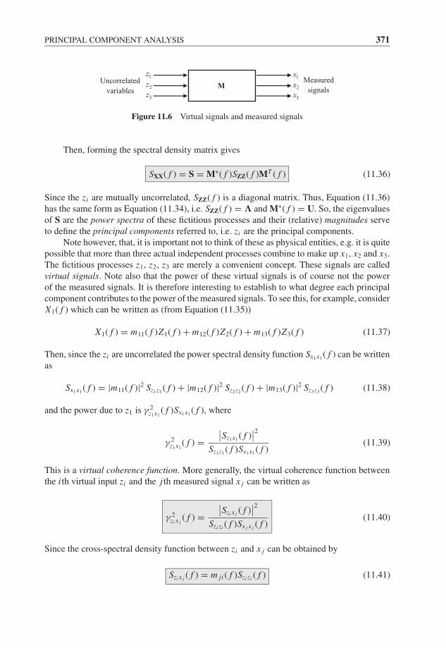
JWBK207-11 JWBK207-Shin January 18, 2008 8:21 Char Count= 0
PRINCIPAL COMPONENT ANALYSIS 371
M1x1z
2x2z
3x3z
Uncorrelated
variables
Measured
signals
Figure 11.6 Virtual signals and measured signals
Then, forming the spectral density matrix gives
SXX( f ) = S = M∗( f )SZZ( f )MT ( f ) (11.36)
Since the zi are mutually uncorrelated, SZZ( f ) is a diagonal matrix. Thus, Equation (11.36)has the same form as Equation (11.34), i.e. SZZ( f ) = Λ and M∗( f ) = U. So, the eigenvaluesof S are the power spectra of these fictitious processes and their (relative) magnitudes serveto define the principal components referred to, i.e. zi are the principal components.
Note however, that, it is important not to think of these as physical entities, e.g. it is quitepossible that more than three actual independent processes combine to make up x1, x2 and x3.The fictitious processes z1, z2, z3 are merely a convenient concept. These signals are calledvirtual signals. Note also that the power of these virtual signals is of course not the powerof the measured signals. It is therefore interesting to establish to what degree each principalcomponent contributes to the power of the measured signals. To see this, for example, considerX1( f ) which can be written as (from Equation (11.35))
X1( f ) = m11( f )Z1( f ) + m12( f )Z2( f ) + m13( f )Z3( f ) (11.37)
Then, since the zi are uncorrelated the power spectral density function Sx1x1( f ) can be written
as
Sx1x1( f ) = |m11( f )|2 Sz1z1
( f ) + |m12( f )|2 Sz2z2( f ) + |m13( f )|2 Sz3z3
( f ) (11.38)
and the power due to z1 is γ 2z1x1
( f )Sx1x1( f ), where
γ 2z1x1
( f ) =∣∣Sz1x1
( f )∣∣2
Sz1z1( f )Sx1x1
( f )(11.39)
This is a virtual coherence function. More generally, the virtual coherence function betweenthe i th virtual input zi and the j th measured signal x j can be written as
γ 2zi x j
( f ) =∣∣Szi x j ( f )
∣∣2
Szi zi ( f )Sx j x j ( f )(11.40)
Since the cross-spectral density function between zi and x j can be obtained by
Szi x j ( f ) = m ji ( f )Szi zi ( f ) (11.41)
JWBK207-11 JWBK207-Shin January 18, 2008 8:21 Char Count= 0
372 MULTIPLE-INPUT/RESPONSE SYSTEMS
we see that the virtual coherence function: (i) can be computed from the eigenvalues andeigenvectors of S; (ii) gives a measure of what proportion of Sx j x j ( f ) comes from a particularcomponent of zi .
For the details of practical applications of principal component analysis, especially fornoise source identification problems, see Otte et al. (1988).
Relationship to the System Identification Methods1
It is interesting to relate principal component analysis (PCA) to the system identificationmethods we described in Chapter 9. Let x denote a column vector of observations (e.g. x(input) and y (output) in Figure 9.9 in Chapter 9) with correlation matrix
Rxx = E[xxT
](11.42)
Let x be derived from a set of uncorrelated processes z (through the transformation matrix T)by
x = Tz (11.43)
Then, the correlation matrix is
Rxx = TE[zzT
]TT = TRzzTT (11.44)
Since the elements of z are uncorrelated, Rzz = Λ, where Λ is a diagonal matrix that containseigenvalues of Rxx. So,
Rxx = T Λ TT (11.45)
This is an eigendecomposition of the correlation matrix Rxx, and T is an orthogonal matrixwhose columns are the corresponding eigenvectors, i.e.
T = [t1 t2
] =[
t11 t12
t21 t22
](11.46)
Let us apply this to the pair of variables (x (input) and y (output)) as in Figure 9.9 inChapter 9. Assuming zero mean values, the correlation matrix is
Rxx = E
[[x
y
] [x y
]] =[
E [xx] E [xy]
E [xy] E [yy]
]=
[σ 2
x σxy
σxy σ 2y
](11.47)
The eigenvalues are
det(Rxx − λI) =∣∣∣∣σ 2
x − λ σxy
σxy σ 2y − λ
∣∣∣∣ = 0 (11.48)
i.e.
λ1,2 =σ 2
x + σ 2y ±
√(σ 2
x − σ 2y
)2 + 4σ 2xy
2(11.49)
1 See Tan (2005).
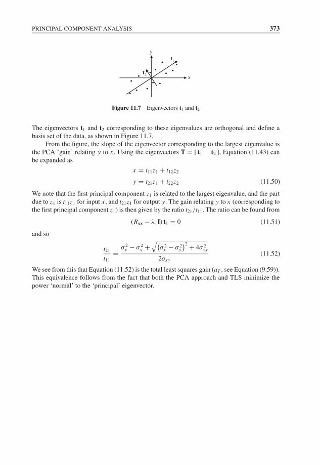
JWBK207-11 JWBK207-Shin January 18, 2008 8:21 Char Count= 0
PRINCIPAL COMPONENT ANALYSIS 373
x
y
1t
2t
Figure 11.7 Eigenvectors t1 and t2
The eigenvectors t1 and t2 corresponding to these eigenvalues are orthogonal and define abasis set of the data, as shown in Figure 11.7.
From the figure, the slope of the eigenvector corresponding to the largest eigenvalue isthe PCA ‘gain’ relating y to x . Using the eigenvectors T = [ t1 t2 ], Equation (11.43) canbe expanded as
x = t11z1 + t12z2
y = t21z1 + t22z2 (11.50)
We note that the first principal component z1 is related to the largest eigenvalue, and the partdue to z1 is t11z1 for input x , and t21z1 for output y. The gain relating y to x (corresponding tothe first principal component z1) is then given by the ratio t21/t11. The ratio can be found from
(Rxx − λ1I) t1 = 0 (11.51)
and so
t21
t11
=σ 2
y − σ 2x +
√(σ 2
x − σ 2y
)2 + 4σ 2xy
2σxy(11.52)
We see from this that Equation (11.52) is the total least squares gain (aT , see Equation (9.59)).This equivalence follows from the fact that both the PCA approach and TLS minimize thepower ‘normal’ to the ‘principal’ eigenvector.

JWBK207-11 JWBK207-Shin January 18, 2008 8:21 Char Count= 0
374
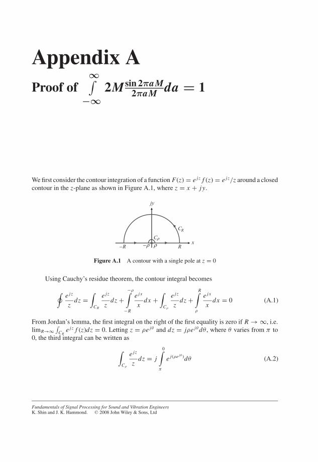
Appendix˙A JWBK207-Shin January 18, 2008 8:21 Char Count= 0
Appendix AProof of
∞∫−∞
2M sin 2πaM2πaM da = 1
We first consider the contour integration of a function F(z) = e jz f (z) = e jz/z around a closedcontour in the z-plane as shown in Figure A.1, where z = x + j y.
x
jy
RC
Cρ
ρ− ρ RR−
Figure A.1 A contour with a single pole at z = 0
Using Cauchy’s residue theorem, the contour integral becomes
∮e jz
zdz =
∫CR
e jz
zdz +
−ρ∫−R
e jx
xdx +
∫Cρ
e jz
zdz +
R∫ρ
e jx
xdx = 0 (A.1)
From Jordan’s lemma, the first integral on the right of the first equality is zero if R → ∞, i.e.limR→∞
∫CR
e jz f (z)dz = 0. Letting z = ρe jθ and dz = jρe jθdθ , where θ varies from π to0, the third integral can be written as∫
Cρ
e jz
zdz = j
0∫π
e j(ρe jθ )dθ (A.2)
Fundamentals of Signal Processing for Sound and Vibration EngineersK. Shin and J. K. Hammond. C© 2008 John Wiley & Sons, Ltd
375

Appendix˙A JWBK207-Shin January 18, 2008 8:21 Char Count= 0
376 APPENDIX A
Taking the limit as ρ → 0, this becomes
limρ→0
⎧⎨⎩ j
0∫π
e j(ρe jθ )dθ
⎫⎬⎭ = jθ|0π = − jπ (A.3)
Now, consider the second and fourth integral together:
−ρ∫−R
e jx
xdx +
R∫ρ
e jx
xdx =
−ρ∫−R
cos x + j sin x
xdx +
R∫ρ
cos x + j sin x
xdx (A.4)
Since cos(x)/x is odd, the cosine terms cancel in the resulting integration. Thus, Equation(A.4) becomes
−ρ∫−R
e jx
xdx +
R∫ρ
e jx
xdx = 2 j
R∫ρ
sin x
xdx (A.5)
Combining the above results, for R → ∞ and ρ → 0, Equation (A.1) reduces to
limρ→0R→∞
⎧⎨⎩2 j
R∫ρ
sin x
xdx
⎫⎬⎭ = 2 j
∞∫0
sin x
xdx = jπ (A.6)
Thus, we have the following result:
∞∫0
sin x
xdx = π
2(A.7)
We now go back to our problem. We have written
limM→∞
2Msin 2πaM
2πaM= δ(a)
in Chapter 3. In order to justify this, the integral of the function
f (a) = 2Msin 2πaM
2πaM
must be unity. We verify this using the above result. Letting x = 2πaM and dx = 2πMda,we have
∞∫−∞
f (a)da =∞∫
−∞2M
sin 2πaM
2πaMda =
∞∫−∞
2Msin x
x
dx
2π M= 1
π
∞∫−∞
sin x
xdx (A.8)
From Equation (A.7),
∞∫−∞
sin x
xdx = 2
∞∫0
sin x
xdx = π
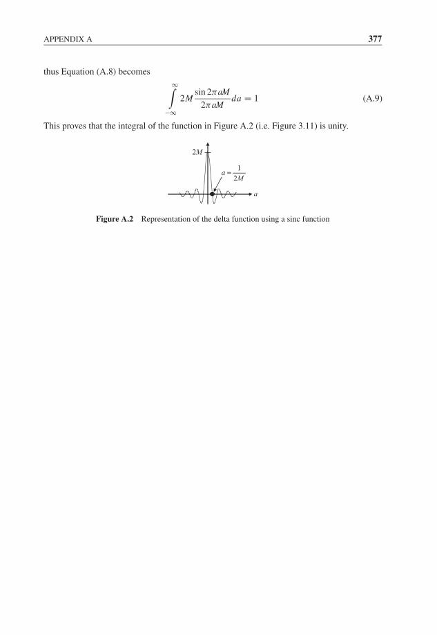
Appendix˙A JWBK207-Shin January 18, 2008 8:21 Char Count= 0
APPENDIX A 377
thus Equation (A.8) becomes
∞∫−∞
2Msin 2πaM
2πaMda = 1 (A.9)
This proves that the integral of the function in Figure A.2 (i.e. Figure 3.11) is unity.
1
2Ma =
a
2M
Figure A.2 Representation of the delta function using a sinc function

Appendix˙A JWBK207-Shin January 18, 2008 8:21 Char Count= 0
378
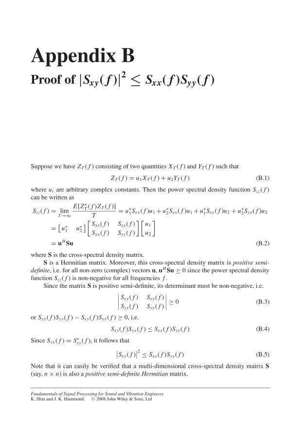
JWBK207-APP-B JWBK207-Shin January 18, 2008 8:21 Char Count= 0
Appendix BProof of |Sxy( f )|2 ≤ Sxx( f )Syy( f )
Suppose we have ZT ( f ) consisting of two quantities XT ( f ) and YT ( f ) such that
ZT ( f ) = u1 XT ( f ) + u2YT ( f ) (B.1)
where ui are arbitrary complex constants. Then the power spectral density function Szz( f )can be written as
Szz( f ) = limT →∞
E[Z∗T ( f )ZT ( f )]
T= u∗
1 Sxx ( f )u1 + u∗2 Syx ( f )u1 + u∗
1 Sxy( f )u2 + u∗2 Syy( f )u2
= [u∗
1 u∗2
] [Sxx ( f ) Sxy( f )
Syx ( f ) Syy( f )
] [u1
u2
]= uH Su (B.2)
where S is the cross-spectral density matrix.S is a Hermitian matrix. Moreover, this cross-spectral density matrix is positive semi-
definite, i.e. for all non-zero (complex) vectors u, uH Su ≥ 0 since the power spectral densityfunction Szz( f ) is non-negative for all frequencies f .
Since the matrix S is positive semi-definite, its determinant must be non-negative, i.e.∣∣∣∣ Sxx ( f ) Sxy( f )
Syx ( f ) Syy( f )
∣∣∣∣ ≥ 0 (B.3)
or Sxx ( f )Syy( f ) − Sxy( f )Syx ( f ) ≥ 0, i.e.
Sxy( f )Syx ( f ) ≤ Sxx ( f )Syy( f ) (B.4)
Since Syx ( f ) = S∗xy( f ), it follows that∣∣Sxy( f )
∣∣2 ≤ Sxx ( f )Syy( f ) (B.5)
Note that it can easily be verified that a multi-dimensional cross-spectral density matrix S(say, n × n) is also a positive semi-definite Hermitian matrix.
Fundamentals of Signal Processing for Sound and Vibration EngineersK. Shin and J. K. Hammond. C© 2008 John Wiley & Sons, Ltd
379

JWBK207-APP-B JWBK207-Shin January 18, 2008 8:21 Char Count= 0
380
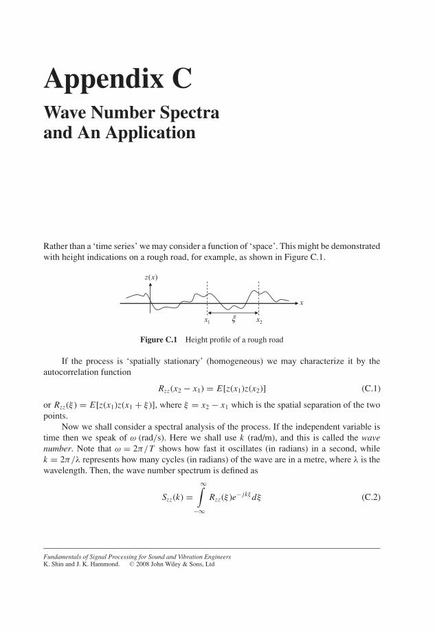
JWBK207-APP-C JWBK207-Shin January 18, 2008 8:23 Char Count= 0
Appendix CWave Number Spectraand An Application
Rather than a ‘time series’ we may consider a function of ‘space’. This might be demonstratedwith height indications on a rough road, for example, as shown in Figure C.1.
( )z x
1x 2xξ
x
Figure C.1 Height profile of a rough road
If the process is ‘spatially stationary’ (homogeneous) we may characterize it by theautocorrelation function
Rzz(x2 − x1) = E[z(x1)z(x2)] (C.1)
or Rzz(ξ ) = E[z(x1)z(x1 + ξ )], where ξ = x2 − x1 which is the spatial separation of the twopoints.
Now we shall consider a spectral analysis of the process. If the independent variable istime then we speak of ω (rad/s). Here we shall use k (rad/m), and this is called the wavenumber. Note that ω = 2π/T shows how fast it oscillates (in radians) in a second, whilek = 2π/λ represents how many cycles (in radians) of the wave are in a metre, where λ is thewavelength. Then, the wave number spectrum is defined as
Szz(k) =∞∫
−∞Rzz(ξ )e− jkξ dξ (C.2)
Fundamentals of Signal Processing for Sound and Vibration EngineersK. Shin and J. K. Hammond. C© 2008 John Wiley & Sons, Ltd
381
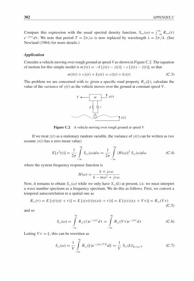
JWBK207-APP-C JWBK207-Shin January 18, 2008 8:23 Char Count= 0
382 APPENDIX C
Compare this expression with the usual spectral density function, Sxx (ω) = ∫ ∞−∞ Rxx (τ )
e− jωτ dτ . We note that period T = 2π/ω is now replaced by wavelength λ = 2π/k. (SeeNewland (1984) for more details.)
Application
Consider a vehicle moving over rough ground at speed V as shown in Figure C.2. The equationof motion for this simple model is my(t) = −k [y(t) − z(t)] − c [y(t) − z(t)], so that
my(t) + cy(t) + ky(t) = cz(t) + kz(t) (C.3)
The problem we are concerned with is: given a specific road property Rzz(ξ ), calculate thevalue of the variance of y(t) as the vehicle moves over the ground at constant speed V .
m
k c
( )y tV
( )z t
Figure C.2 A vehicle moving over rough ground at speed V
If we treat z(t) as a stationary random variable, the variance of y(t) can be written as (weassume y(t) has a zero mean value)
E[y2(t)] = 1
2π
∞∫−∞
Syy(ω)dω = 1
2π
∞∫−∞
|H (ω)|2 Szz(ω)dω (C.4)
where the system frequency response function is
H (ω) = k + jcω
k − mω2 + jcω
Now, it remains to obtain Szz(ω) while we only have Szz(k) at present, i.e. we must interpreta wave number spectrum as a frequency spectrum. We do this as follows. First, we convert atemporal autocorrelation to a spatial one as
Rzz(τ ) = E [z(t)z(t + τ )] = E [z(x(t))z(x(t + τ ))] = E [z(x)z(x + V τ )] = Rzz(V τ )(C.5)
and so
Szz(ω) =∞∫
−∞Rzz(τ )e− jωτ dτ =
∞∫−∞
Rzz(V τ )e− jωτ dτ (C.6)
Letting V τ = ξ , this can be rewritten as
Szz(ω) = 1
V
∞∫−∞
Rzz(ξ )e− j(ω/V )ξ dξ = 1
VSzz(k)|k=ω/V (C.7)
JWBK207-APP-C JWBK207-Shin January 18, 2008 8:23 Char Count= 0
APPENDIX C 383
Thus, to obtain the frequency spectrum from the wave number spectrum we simply replace kby ω/V and divide by V . Note that the speed can be expressed by
V = f λ = ω
2πλ = ω
k
For a simple example, if the road property is Rzz(ξ ) = e−0.2|ξ | then the wave numberspectrum and the power spectral density function are
Szz(k) = 0.4
0.04 + k2and Szz(ω) = 0.4V
0.04V 2 + ω2
respectively.

JWBK207-APP-C JWBK207-Shin January 18, 2008 8:23 Char Count= 0
384
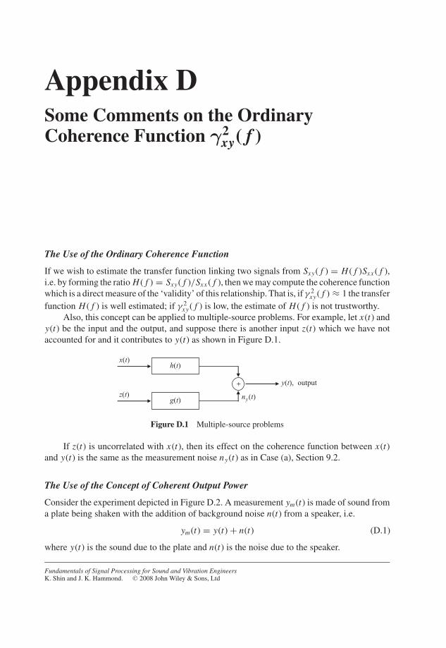
JWBK207-APP-D JWBK207-Shin January 18, 2008 8:23 Char Count= 0
Appendix DSome Comments on the OrdinaryCoherence Function γ2
xy( f )
The Use of the Ordinary Coherence Function
If we wish to estimate the transfer function linking two signals from Sxy( f ) = H ( f )Sxx ( f ),i.e. by forming the ratio H ( f ) = Sxy( f )/Sxx ( f ), then we may compute the coherence functionwhich is a direct measure of the ‘validity’ of this relationship. That is, if γ 2
xy( f ) ≈ 1 the transfer
function H ( f ) is well estimated; if γ 2xy( f ) is low, the estimate of H ( f ) is not trustworthy.
Also, this concept can be applied to multiple-source problems. For example, let x(t) andy(t) be the input and the output, and suppose there is another input z(t) which we have notaccounted for and it contributes to y(t) as shown in Figure D.1.
x(t)
+
(t)yn
y(t), output
h(t)
z(t)g(t)
Figure D.1 Multiple-source problems
If z(t) is uncorrelated with x(t), then its effect on the coherence function between x(t)and y(t) is the same as the measurement noise ny(t) as in Case (a), Section 9.2.
The Use of the Concept of Coherent Output Power
Consider the experiment depicted in Figure D.2. A measurement ym(t) is made of sound froma plate being shaken with the addition of background noise n(t) from a speaker, i.e.
ym(t) = y(t) + n(t) (D.1)
where y(t) is the sound due to the plate and n(t) is the noise due to the speaker.
Fundamentals of Signal Processing for Sound and Vibration EngineersK. Shin and J. K. Hammond. C© 2008 John Wiley & Sons, Ltd
385
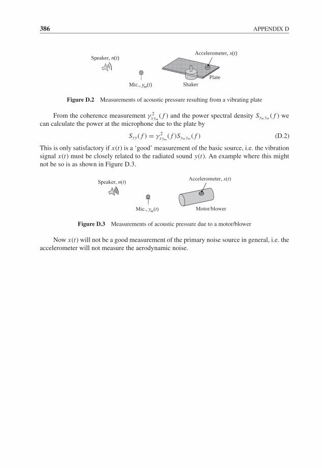
JWBK207-APP-D JWBK207-Shin January 18, 2008 8:23 Char Count= 0
386 APPENDIX D
Speaker, n(t)
Mic., ym(t) Shaker
Accelerometer, x(t)
Plate
Figure D.2 Measurements of acoustic pressure resulting from a vibrating plate
From the coherence measurement γ 2xym
( f ) and the power spectral density Sym ym ( f ) wecan calculate the power at the microphone due to the plate by
Syy( f ) = γ 2xym
( f )Sym ym ( f ) (D.2)
This is only satisfactory if x(t) is a ‘good’ measurement of the basic source, i.e. the vibrationsignal x(t) must be closely related to the radiated sound y(t). An example where this mightnot be so is as shown in Figure D.3.
Speaker, n(t)
Mic., ym(t) Motor/blower
Accelerometer, x(t)
Figure D.3 Measurements of acoustic pressure due to a motor/blower
Now x(t) will not be a good measurement of the primary noise source in general, i.e. theaccelerometer will not measure the aerodynamic noise.
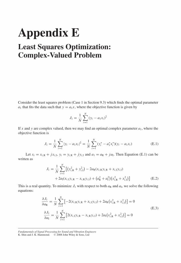
Appendix˙E JWBK207-Shin January 18, 2008 8:23 Char Count= 0
Appendix ELeast Squares Optimization:Complex-Valued Problem
Consider the least squares problem (Case 1 in Section 9.3) which finds the optimal parametera1 that fits the data such that y = a1x , where the objective function is given by
J1 = 1
N
N∑i=1
(yi − a1xi )2
If x and y are complex valued, then we may find an optimal complex parameter a1, where theobjective function is
J1 = 1
N
N∑i=1
|yi − a1xi |2 = 1
N
N∑i=1
(y∗i − a∗
1 x∗i )(yi − a1xi ) (E.1)
Let xi = xi,R + j xi,I, yi = yi,R + j yi,I and a1 = aR + jaI. Then Equation (E.1) can bewritten as
J1 = 1
N
N∑i=1
[(y2
i,R + y2i,I
) − 2aR(xi,R yi,R + xi,I yi,I)
+ 2aI(xi,I yi,R − xi,R yi,I) + (a2
R + a2I
)(x2
i,R + x2i,I
)](E.2)
This is a real quantity. To minimize J1 with respect to both aR and aI, we solve the followingequations:
∂ J1
∂aR
= 1
N
N∑i=1
[−2(xi,R yi,R + xi,I yi,I) + 2aR
(x2
i,R + x2i,I
)] = 0
∂ J1
∂aI
= 1
N
N∑i=1
[2(xi,I yi,R − xi,R yi,I) + 2aI
(x2
i,R + x2i,I
)] = 0
(E.3)
Fundamentals of Signal Processing for Sound and Vibration EngineersK. Shin and J. K. Hammond. C© 2008 John Wiley & Sons, Ltd
387
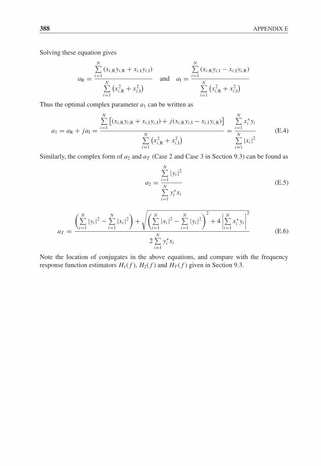
Appendix˙E JWBK207-Shin January 18, 2008 8:23 Char Count= 0
388 APPENDIX E
Solving these equation gives
aR =
N∑i=1
(xi,R yi,R + xi,I yi,I)
N∑i=1
(x2
i,R + x2i,I
) and aI =
N∑i=1
(xi,R yi,I − xi,I yi,R)
N∑i=1
(x2
i,R + x2i,I
)Thus the optimal complex parameter a1 can be written as
a1 = aR + jaI =
N∑i=1
[(xi,R yi,R + xi,I yi,I) + j(xi,R yi,I − xi,I yi,R)
]N∑
i=1
(x2
i,R + x2i,I
) =
N∑i=1
x∗i yi
N∑i=1
|xi |2(E.4)
Similarly, the complex form of a2 and aT (Case 2 and Case 3 in Section 9.3) can be found as
a2 =
N∑i=1
|yi |2
N∑i=1
y∗i xi
(E.5)
aT =
(N∑
i=1
|yi |2 −N∑
i=1
|xi |2)
+√(
N∑i=1
|xi |2 −N∑
i=1
|yi |2)2
+ 4
∣∣∣∣ N∑i=1
x∗i yi
∣∣∣∣2
2N∑
i=1
y∗i xi
(E.6)
Note the location of conjugates in the above equations, and compare with the frequencyresponse function estimators H1( f ), H2( f ) and HT ( f ) given in Section 9.3.
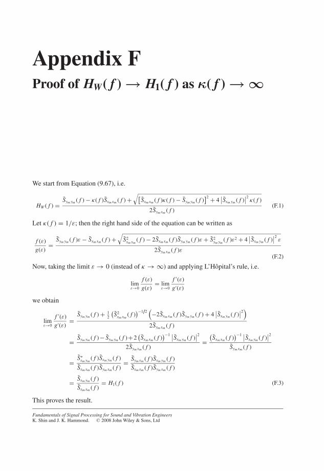
JWBK207-APP-F JWBK207-Shin January 18, 2008 8:24 Char Count= 0
Appendix FProof of HW( f ) → H1( f ) as κ( f ) → ∞
We start from Equation (9.67), i.e.
HW ( f ) =Sym ym ( f ) − κ( f )Sxm xm ( f ) +
√[Sxm xm ( f )κ( f ) − Sym ym ( f )
]2 + 4∣∣Sxm ym ( f )
∣∣2κ( f )
2Sym xm ( f )(F.1)
Let κ( f ) = 1/ε; then the right hand side of the equation can be written as
f (ε)
g(ε)=
Sym ym ( f )ε − Sxm xm ( f ) +√
S2xm xm
( f ) − 2Sxm xm ( f )Sym ym ( f )ε + S2ym ym
( f )ε2 + 4∣∣Sxm ym ( f )
∣∣2ε
2Sym xm ( f )ε(F.2)
Now, taking the limit ε → 0 (instead of κ → ∞) and applying L’Hopital’s rule, i.e.
limε→0
f (ε)
g(ε)= lim
ε→0
f ′(ε)
g′(ε)
we obtain
limε→0
f ′(ε)
g′(ε)=
Sym ym ( f ) + 12
(S2
xm xm( f )
)−1/2(−2Sxm xm ( f )Sym ym ( f ) + 4
∣∣Sxm ym ( f )∣∣2
)2Sym xm ( f )
= Sym ym ( f )− Sym ym ( f )+2(Sxm xm ( f )
)−1 ∣∣Sxm ym ( f )∣∣2
2Sym xm ( f )=
(Sxm xm ( f )
)−1 ∣∣Sxm ym ( f )∣∣2
Sym xm ( f )
= S∗xm ym
( f )Sxm ym ( f )
Sxm xm ( f )Sym xm ( f )= Sym xm ( f )Sxm ym ( f )
Sxm xm ( f )Sym xm ( f )
= Sxm ym ( f )
Sxm xm ( f )= H1( f ) (F.3)
This proves the result.
Fundamentals of Signal Processing for Sound and Vibration EngineersK. Shin and J. K. Hammond. C© 2008 John Wiley & Sons, Ltd
389

JWBK207-APP-F JWBK207-Shin January 18, 2008 8:24 Char Count= 0
390
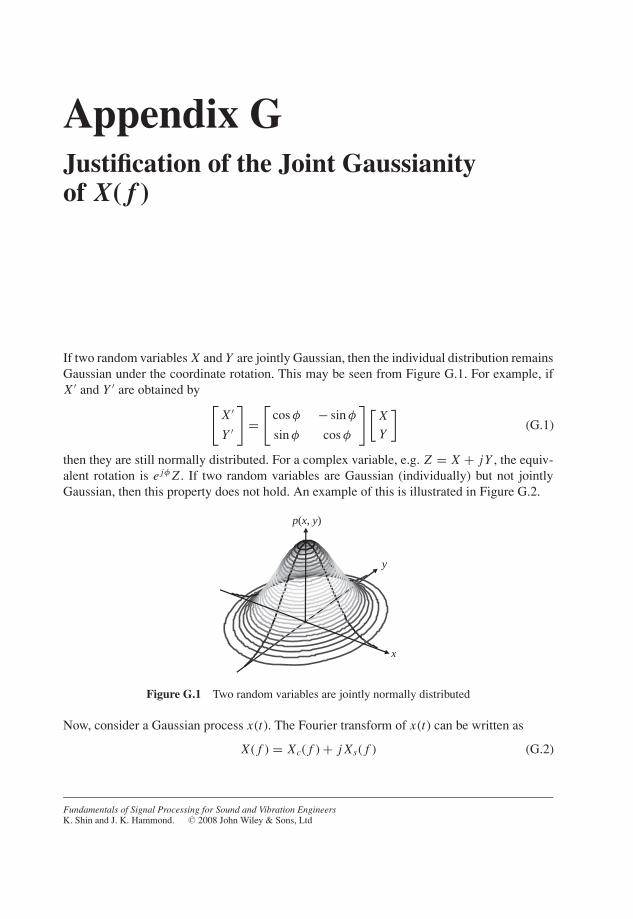
JWBK207-APP-G JWBK207-Shin January 18, 2008 8:24 Char Count= 0
Appendix GJustification of the Joint Gaussianityof X( f )
If two random variables X and Y are jointly Gaussian, then the individual distribution remainsGaussian under the coordinate rotation. This may be seen from Figure G.1. For example, ifX ′ and Y ′ are obtained by [
X ′
Y ′
]=
[cos φ − sin φ
sin φ cos φ
] [X
Y
](G.1)
then they are still normally distributed. For a complex variable, e.g. Z = X + jY , the equiv-alent rotation is e jφ Z . If two random variables are Gaussian (individually) but not jointlyGaussian, then this property does not hold. An example of this is illustrated in Figure G.2.
x
y
p(x, y)
Figure G.1 Two random variables are jointly normally distributed
Now, consider a Gaussian process x(t). The Fourier transform of x(t) can be written as
X ( f ) = Xc( f ) + j Xs( f ) (G.2)
Fundamentals of Signal Processing for Sound and Vibration EngineersK. Shin and J. K. Hammond. C© 2008 John Wiley & Sons, Ltd
391

JWBK207-APP-G JWBK207-Shin January 18, 2008 8:24 Char Count= 0
392 APPENDIX G
p(x, y)
x
y
Figure G.2 Each random variable is normally distributed, but not jointly
where Xc( f ) and Xs( f ) are Gaussian since x(t) is Gaussian. If these are jointly Gaussian, theymust remain Gaussian under the coordinate rotation (for any rotation angle φ). For example,if e jφ X ( f ) = X ′( f ) = X ′
c( f ) + j X ′s( f ) then X ′
c( f ) and X ′s( f ) must be Gaussian, where
X ′c( f ) = Xc( f ) cos φ − Xs( f ) sin φ and X ′
s( f ) = Xc( f ) sin φ + Xs( f ) cos φ.For a particular frequency f , let φ = −2π f t0. Then e− j2π f t0 X ( f ) is a pure delay, i.e.
x(t − t0) in the time domain for that frequency component. If we assume that x(t) is a sta-tionary Gaussian process, then x(t − t0) is also Gaussian, so both X ′
c( f ) and X ′s( f ) remain
Gaussian under the coordinate rotation. This justifies that Xc( f ) and Xs( f ) are jointly normallydistributed.
JWBK207-APP-H JWBK207-Shin January 18, 2008 8:25 Char Count= 0
Appendix HSome Comments on Digital Filtering
We shall briefly introduce some terminology and methods of digital filtering that may beuseful. There are many good texts on this subject: for example, Childers and Durling (1975),Oppenheim and Schafer (1975), Oppenheim et al. (1999) and Rabiner and Gold (1975). Also,sound and vibration engineers may find some useful concepts in White and Hammond (2004)together with some other advanced topics in signal processing.
The reason for including this subject is because we have used some digital filteringtechniques through various MATLAB examples, and also introduced some basic concepts inChapter 6 when we discussed a digital LTI system, i.e. the input–output relationship for adigital system that can be expressed by
y(n) = −N∑
k=1
ak y(n − k) +M∑
r=0
br x(n − r ) (H.1)
where x(n) denotes an input sequence and y(n) the output sequence. This difference equationis the general form of a digital filter which can easily be programmed to produce an outputsequence for a given input sequence. The z-transform may be used to solve this equation andto find the transfer function which is given by
H (z) = Y (z)
X (z)=
M∑r=0
br z−r
1 +N∑
k=1ak z−k
(H.2)
By appropriate choice of the coefficients ak and br and the orders N and M , the characteristicsof H (z) can be adjusted to some desired form. Note that, since we are using a finite wordlength in the computation, the coefficients cannot be represented exactly. This will introducesome arithmetic round-off error.
Fundamentals of Signal Processing for Sound and Vibration EngineersK. Shin and J. K. Hammond. C© 2008 John Wiley & Sons, Ltd
393
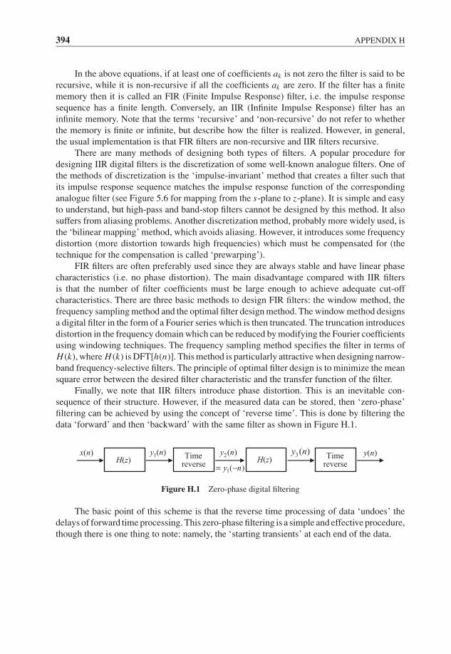
JWBK207-APP-H JWBK207-Shin January 18, 2008 8:25 Char Count= 0
394 APPENDIX H
In the above equations, if at least one of coefficients ak is not zero the filter is said to berecursive, while it is non-recursive if all the coefficients ak are zero. If the filter has a finitememory then it is called an FIR (Finite Impulse Response) filter, i.e. the impulse responsesequence has a finite length. Conversely, an IIR (Infinite Impulse Response) filter has aninfinite memory. Note that the terms ‘recursive’ and ‘non-recursive’ do not refer to whetherthe memory is finite or infinite, but describe how the filter is realized. However, in general,the usual implementation is that FIR filters are non-recursive and IIR filters recursive.
There are many methods of designing both types of filters. A popular procedure fordesigning IIR digital filters is the discretization of some well-known analogue filters. One ofthe methods of discretization is the ‘impulse-invariant’ method that creates a filter such thatits impulse response sequence matches the impulse response function of the correspondinganalogue filter (see Figure 5.6 for mapping from the s-plane to z-plane). It is simple and easyto understand, but high-pass and band-stop filters cannot be designed by this method. It alsosuffers from aliasing problems. Another discretization method, probably more widely used, isthe ‘bilinear mapping’ method, which avoids aliasing. However, it introduces some frequencydistortion (more distortion towards high frequencies) which must be compensated for (thetechnique for the compensation is called ‘prewarping’).
FIR filters are often preferably used since they are always stable and have linear phasecharacteristics (i.e. no phase distortion). The main disadvantage compared with IIR filtersis that the number of filter coefficients must be large enough to achieve adequate cut-offcharacteristics. There are three basic methods to design FIR filters: the window method, thefrequency sampling method and the optimal filter design method. The window method designsa digital filter in the form of a Fourier series which is then truncated. The truncation introducesdistortion in the frequency domain which can be reduced by modifying the Fourier coefficientsusing windowing techniques. The frequency sampling method specifies the filter in terms ofH (k), where H (k) is DFT[h(n)]. This method is particularly attractive when designing narrow-band frequency-selective filters. The principle of optimal filter design is to minimize the meansquare error between the desired filter characteristic and the transfer function of the filter.
Finally, we note that IIR filters introduce phase distortion. This is an inevitable con-sequence of their structure. However, if the measured data can be stored, then ‘zero-phase’filtering can be achieved by using the concept of ‘reverse time’. This is done by filtering thedata ‘forward’ and then ‘backward’ with the same filter as shown in Figure H.1.
x(n)H(z)
1(n)y Timereverse
2(n)yH(z)
1 )(y −n=
3(n)y y(n)Timereverse
Figure H.1 Zero-phase digital filtering
The basic point of this scheme is that the reverse time processing of data ‘undoes’ thedelays of forward time processing. This zero-phase filtering is a simple and effective procedure,though there is one thing to note: namely, the ‘starting transients’ at each end of the data.

JWBK207-REF JWBK207-Shin January 18, 2008 8:25 Char Count= 0
References
Ables, J. G., ‘Maximum entropy spectral analysis’, Astronomy and Astrophysics Supplement Series,Vol. 15, pp. 383–393, 1974.
Allemang, R. J. and Brown, D. L., ‘Experimental modal analysis’, Chapter 21, in Harris’ Shock andVibration Handbook, Fifth Edition, ed. Harris, C. M. and Piersol, A. G., McGraw-Hill, 2002.
Bencroft, J. C., ‘Introduction to matched filters’, CREWES Research Report, Vol. 14, pp. 1–14, 2002.Bendat, J. S., ‘Solutions for the multiple input/output problem’, Journal of Sound and Vibration, Vol. 44,
No. 3, pp. 311–325, 1976a.Bendat, J. S., ‘System identification from multiple input/output data’, Journal of Sound and Vibration,
Vol. 49, No. 3, pp. 293–208, 1976b.Bendat, J. S., ‘Statistical errors in measurement of coherence functions and input/output quantities’,
Journal of Sound and Vibration, Vol. 59, No. 3, pp. 405–421, 1978.Bendat, J. S. and Piersol, A. G., Engineering Applications of Correlation and Spectral Analysis, John
Wiley & Sons, Inc., 1980.Bendat, J. S. and Piersol, A. G., Random Data: Analysis and Measurement Procedures, Third Edition,
a Wiley-Interscience, 2000.Bingham, C., Godfrey, M. and Tukey, J. W., ‘Modern techniques of power spectrum estimation’, IEEE
Transactions on Audio and Electroacoustics, Vol. AU-15, No. 2, pp. 56–66, 1967.Bogert, B. P., Healey, M. J. R. and Tukey, J. W., ‘The quefrency analysis of time series for echoes:
cepstrum, pseudo-autocovariance, cross-cepstrum and saphe cracking’, Proceedings of the Sympo-sium on Time Series Analysis, ed. Rosenblatt, Murray, pp. 209–243, John Wiley and Sons, Inc.,1963.
Brigham, E. O., The Fast Fourier Transform and Its Applications, Prentice Hall, 1988.Carter, G. C., Knapp, C. H. and Nuttall, A. H., ‘Estimation of the magnitude-squared coherence function
via overlapped fast Fourier transform processing’, IEEE Transactions on Audio and Electroacoustics,Vol. AU-21, No. 4, pp. 337–344, 1973.
Childers, D. and Durling, A., Digital Filtering and Signal Processing, West Publishing, 1975.Cohen, L., ‘Time-frequency distributions – a review’, Proceedings of the IEEE, Vol. 77, No. 7,
pp. 941–981, 1989.Cooley, J. W. and Tukey J. W., ‘An algorithm for the machine computation of complex Fourier series’,
Mathematics of Computation, Vol. 19, pp. 297–301, 1965.
Fundamentals of Signal Processing for Sound and Vibration EngineersK. Shin and J. K. Hammond. C© 2008 John Wiley & Sons, Ltd
395

JWBK207-REF JWBK207-Shin January 18, 2008 8:25 Char Count= 0
396 REFERENCES
Davies, P., ‘A recursive approach to Prony parameter estimation’, Journal of Sound and Vibration,Vol. 89, No. 4, pp. 571–583, 1983.
de Prony, B. G. R., ‘Essai experimental et analytique: sur les lois de la dilatabilite de fluides elastiqueet sur celles de la force expansive de la vapeur de l’alkool, a differentes temperatures’, Journal del’Ecole Polytechnique, Vol. 1, cahier 22, pp. 24–76, 1795.
Duhamel, P. and Vetterli, M., ‘Fast Fourier transforms: a tutorial review and a state of the art’, SignalProcessing, Vol. 19, pp. 259–299, 1990.
Fahy, F. and Walker, J., Fundamentals of Noise and Vibration, Spon Press, 1998.Gao, Y., Brennan, M. J. and Joseph, P. H., ‘A comparison of time delay estimator for the detection
of leak noise signal in plastic water distribution pipes’, Journal of Sound and Vibration, Vol. 292,pp. 552–570, 2006.
Hammond, J. K. and White, P. R., ‘The analysis of non-stationary signals using time-frequency methods’,Journal of Sound and Vibration, Vol. 190, No. 3, pp. 419–447, 1996.
Harris, F. J., ‘On the use of windows for harmonic analysis with the discrete Fourier transform’, Pro-ceedings of the IEEE, Vol. 66, No. 1, pp. 51–83, 1978.
Hsu, Hwei P., Fourier Analysis, Revised Edition, Simon & Schuster, 1970.Jenkins, G. M. and Watts, D. G., Spectral Analysis and its Applications, Holden-Day, 1968.Kay, S. M. and Marple Jr, S. L., ‘Spectrum analysis – a modern perspective’, Proceedings of the IEEE,
Vol. 69, No. 11, pp. 1380–1419, 1981.Lee, Y.-S., ‘Active control of smart structures using distributed piezoelectric Transducers’, PhD Thesis,
Institute of Sound and Vibration Research, University of Southampton, 2000.Leuridan, J., De Vis, D., Van der Auweraer, H. and Lembregts, F., ‘A comparison of some frequency
response function measurement techniques’, Proceedings of the 4th International Modal AnalysisConference IMAC, Los Angeles, CA, pp. 908–918, 1986.
Levi, E. C., ‘Complex-curve fitting’, IRE Transactions on Automatic Control, Vol. AC/4, pp. 37–43,1959.
Marple Jr, S. L., Digital Spectral Analysis with Applications, Prentice Hall, 1987.Newland, D. E., An Introduction to Random Vibrations and Spectral Analysis, Longman Scientific &
Technical, 1984.Oppenheim, A. V. and Schafer, R. W., Digital Signal Processing, Prentice Hall International, 1975.Oppenheim, A. V., Willsky, A. S. and Hamid Nawab, S., Signals & Systems, Second Edition, Prentice
Hall International, 1997.Oppenheim, A. V., Schafer, R. W. and Buck, J. R., Discrete-Time Signal Processing, Second Edition,
Prentice Hall International, 1999.Otnes, R. K. and Enochson, L., Applied Time Series Analysis Vol. 1. Basic Techniques, John Wiley and
Sons, Inc., 1978.Otte, D., Fyfe, K., Sas, P. and Leuridan, J., ‘Use of principal component analysis for dominant
noise source identification’, Proceedings of the Institution of Mechanical Engineers, InternationalConference: Advances in the Control and Refinement of Vehicle Noise, C21/88, pp. 123–132,1988.
Papoulis, A., Signal Analysis, McGraw-Hill, 1977.Papoulis, A., Probability, Random Variables, and Stochastic Processes, McGraw-Hill, 1991.Priestley, M. B., Spectral Analysis and Time Series, Academic Press, 1981.Proakis, J. G. and Manolakis, D. G., Introduction to Digital Signal Processing, Macmillan, 1988.Rabiner, L. R. and Gold, B., Theory and Applications of Digital Signal Processing, Prentice Hall,
1975.Randall, R. B., Frequency Analysis, Third Edition, Bruel and Kjaer, 1987.Schmidt, H., ‘Resolution bias errors in spectral density, frequency response and coherence function
measurement, III: application to second-order systems (white noise excitation)’, Journal of Soundand Vibration, Vol. 101, No. 3, pp. 377–404, 1985a.
JWBK207-REF JWBK207-Shin January 18, 2008 8:25 Char Count= 0
REFERENCES 397
Schmidt, H., ‘Resolution bias errors in spectral density, frequency response and coherence func-tion measurement, IV: time delay bias errors’, Journal of Sound and Vibration, Vol. 101, No. 3,pp. 405–412, 1985b.
Smith, J. O., Mathematics of the Discrete Fourier Transform (DFT), http://ccrma.stanford.edu/∼jos/mdft/, 2003.
Spitznogle, F. R. and Quazi, A. H., ‘Representation and analysis of time-limited signals using a complexexponential algorithm’, Journal of the Acoustical Society of America, Vol. 47, No. 5(1), pp. 1150–1155, 1970.
Sutton, T. J., Elliot, S. J., McDonald, A. M. and Saunders, T. J., ‘Active control of road noise insidevehicles’, Noise Control Engineering Journal, Vol. 42, No. 4, pp. 137–147, 1994.
Tan, M. H., ‘Principal component analysis for signal-based system identification’, PhD Thesis, Instituteof Sound and Vibration Research, University of Southampton, 2005.
Welch, P. D., ‘The use of fast Fourier transform for the estimation of power spectra: a method based ontime averaging over short, modified periodograms’, IEEE Transactions on Audio and Electroacous-tics, Vol. AU-15, No. 2, pp. 70–73, 1967.
Wellstead, P. E., ‘Non-parametric methods of system identification’, Automatica, Vol. 17, pp. 55–69,1981.
White, P. R. and Hammond, J. K., ‘Signal processing techniques’, Chapter 1, in Advanced Applicationsin Acoustics, Noise and Vibration, ed. Fahy, F. J. and Walker, J. G., Spon Press, 2004.
White, P. R., Tan, M. H. and Hammond, J. K., ‘Analysis of the maximum likelihood, total least squaresand principal component approaches for frequency response function estimation’, Journal of Soundand Vibration, Vol. 290, pp. 676–689, 2006.
Wicks, A. L. and Vold, H., ‘The Hs frequency response function estimator’, Proceedings of the 4thInternational Modal Analysis Conference, IMAC, Los Angeles, CA, pp. 897–899, 1986.
Zadeh, L. A. and Desoer, C. A., Linear System Theory: The State Space Approach, McGraw-Hill, 1963.

JWBK207-REF JWBK207-Shin January 18, 2008 8:25 Char Count= 0
398

JWBK207-IND JWBK207-Shin January 26, 2008 17:31 Char Count= 0
Index
Aliasing, 123, 126–128, 140–144, 181
All-pass filter, see Filter, all-pass
Amplitude Modulation, see Modulation, amplitude
Analogue-to-digital conversion, 131–134
Analogue-to-digital converter (ADC), 130, 131
Analytic signal, 91
Anti-aliasing filter, see Filter, anti-aliasing
Anti-imaging filter, see Filter, reconstruction
Autocorrelation coefficient, 225, 228
Autocorrelation function, 225–227, 231
computational form, 231, 325
estimator, 323
examples, 234–240, 255–258, 259–261, 274
properties, 228
sine wave, 234–235, 255–256
square wave, 238–239
time delay problem, 237–238, 256–258
transient signal, 239–240
via FFT, 325–326
white noise, 236
Autocovariance function, see Autocorrelation function
Auto-regressive (AR), 149
Auto-regressive moving average (ARMA), 149
Band-limited, 128. See also White noise, band-limited
Bandwidth
3 dB, 99, 329, 332
noise, 99, 100, 332
resolution, 340, 341, 342, 344
Bandwidth-time (BT) product, see Uncertainty principle
Bias, 94, 318. See also Error; Estimator errors
Bivariate, 201, 205, 206
Bounded input/bounded output (BIBO) stable, 87, 149
Butterworth, see Filter, low-pass
Causal, 75, 76, 147
Central limit theorem, 205, 213–214
Central moment, see Moment, central
Cepstral analysis, 73
Chebychev, see Filter, low-pass
Chi-squared (χ2n ) distribution, 335–336
Coherence function, 284–287, 385
effect of measurement noise, 285–287
estimator, 349
multiple, 368
partial, 367
virtual, 371
Coherent output power, 286, 385
Confidence interval, 319
spectral estimates, 345–347
Conjugate symmetry property, see Symmetry property
Convolution, 3, 75–77, 147–148, 182–183
circular, see Convolution, periodic
fast, 164
integral, 75–76
linear, see Convolution, sum
periodic, 162–163, 182–183
sequences, see Convolution, sum
sum, 147–148, 164, 170–171, 182–183
Correlation, 206
coefficient, 206, 215–216
Correlation function, see Autocorrelation function;
Cross-correlation function
Cost function, see Objective function
Fundamentals of Signal Processing for Sound and Vibration EngineersK. Shin and J. K. Hammond. C© 2008 John Wiley & Sons, Ltd
399

JWBK207-IND JWBK207-Shin January 26, 2008 17:31 Char Count= 0
400 INDEX
Covariance, 206
Covariance function, see Autocorrelation function;
Cross-correlation function
Cross-correlation coefficient, 228
Cross-correlation function, 227–228, 231
computational form, 231, 325
estimator, 324
examples, 240–242, 258–266, 273–274
properties, 228–229
time delay problem, 241–242, 261–266
Cross-covariance function, see Cross-correlation
function
Cross-spectral density function, 247
estimator, 292, 347, 348
examples, 249–251, 266–275
properties, 247–249
raw, 347, 348
smoothed, 347, 348
time delay problem, 250–251
Cumulative distribution function, see Distribution
function
Cut-off frequency, 129, 130
Data truncation, 94–96, 109–114, 155–156, 158–160,
171–174. See also Fourier series, computational
consideration
Data validation, 136
Decimation in time (DIT), 165
Deconvolution, see Cepstral analysis
Degrees of freedom, 335, 340, 344, 345, 346
Delta function, 38–39, See also Impulse
Dirac delta, 38
Fourier transform, see Fourier integral, Dirac delta;
Discrete Fourier Transform, Kronecker delta
Kronecker delta, 146
properties, 39–40
Deterministic, see Signal, deterministic
Digital filter, see Filter, digital
Digital-to-analogue converter (DAC), 135, 139
Discrete Fourier transform (DFT), 50, 153–155,
156
inverse (IDFT), 51, 154
Kronecker delta, 160
properties, 160–161
scaling effect, 158–160
Dirichlet conditions, see Fourier series, convergence
Dispersion, see Group delay
Distribution function, 199, 200
Dynamic range, 130, 133, 134
Echo, 72–73, 103–104
Ensemble, 220
Ensemble average, 223–224
autocorrelation function, 226–227, 255–256
probability density function, 253–254
Envelope analysis, 91
Ergodic, 229
Error, see also Estimator errors
bias error, 319
random error, 319, 352
RMS error, 319
Estimator errors, 317–320
autocorrelation function, 323–324
coherence function, 349–350, 358–360
cross-correlation function, 324–325
cross-spectral density function, 348–349, 354–358,
360–362
frequency response function, 351–352
mean square value, 321–322
mean value, 320–321
power spectral density function, 327–330, 334–337,
339–342, 343–344, 345, 354–358
table, 352
Even function, 37, 44, 59
Expectation, 202
Expected value, 203. See also Ensemble average
Experiment of chance, 194
Event, 194
algebra, 194–195
equally likely, 194, 196
Fast Fourier transform (FFT), 164–166. See alsoDiscrete Fourier transform
Filter
all-pass, 85
anti-aliasing, 128–131, 143
band-pass, 82
constant bandwidth, 330
constant percentage bandwidth, 331
digital, 148, 393–394
low-pass, 82, 129
octave, 331
reconstruction, 139
third (1/3) octave, 331
Filter bank method, 327. See also Power
spectral density function, estimation
methods
Finite Impulse Response (FIR), 265, 394
Folding frequency, 127
Fourier integral, 57–61
Dirac delta, 62
examples, 62–67
Gaussian pulse, 66
inversion, 60–61
pair, 59, 60
periodic function, 67
properties, 67–71
rectangular pulse, 64
sine function, 63
table, 68
JWBK207-IND JWBK207-Shin January 26, 2008 17:31 Char Count= 0
INDEX 401
Fourier series, 31–34, 41, 42–43. See also Fourier
transform
complex form, 42–43
computational consideration, 46–48, 49, 54–56.
See also Data truncation
convergence, 36
even function, 38
odd function, 38
rectangular pulse, 44–45
relationship with DFT, 48, 50–51
square wave, 34–36, 49
Fourier transform
continuous signal, see Fourier integral
convolution, 70, 152
descrete-time, 152
differentiation, 70
discrete, see Discrete Fourier transform
product, 71
properties, see Fourier integral, properties; Discrete
Fourier transform, properties
sampled sequence, 121, 153
summary, 168–169
train of delta functions, 122
Frequency domain, 20
Frequency modulation, see Modulation, frequency
Frequency response function (FRF), see also System
identification
biasing effect of noise, 294–295, 307–312
continuous system, 4, 77–78
curve fitting, 311–313
descrete (digital) system, 150
estimator H1, 6, 184, 293, 350
estimator H2, 6, 293
estimator H3, see System identification, effect of
feedback
estimator HT , 6, 294
estimator HW , 293
Frequency smoothing, 345. See also Power spectral
density function, estimation methods
Gaussian pulse, see Fourier integral, Gaussian pulse
Gaussian, see Probability distribution, Gaussian
Gibbs’ phenomenon, 36, 52–53
Group delay, 72, 82–85, 104–105
Group velocity, 84
Hilbert transform, 90–93, 106–109
Impulse-invariant, 125, 148
Impulse, see Delta function
Impulse response
continuous, 75
discrete, 147
Impulse train, 41, 42, 119, 120
Independent, see Statistically independent
Infinite Impulse Response (IIR), 125, 394
Instantaneous amplitude, 91
Instantaneous frequency, 91
Instantaneous phase, 91
Inverse spreading property, 63, 64, 101
Kurtosis, 208, 216–218. See also Moment
computational form, 210
Laplace transform, 78, 124. See also z-transform
sampled function, 124, 125
Leakage, 94, 95
Least squares, 289. See also Total least squares
complex valued problem, 387–388
Leptokurtic, see Kurtosis
Linearity, 74
Linear phase, see Pure delay
Linear time-invariant (LTI) system, 73
continuous, 73–81
discrete, 147, 149–150
examples, 78–81
Matched filter, 263
Mean square error, 319. See also Estimator errors
Mean square value, 204, 222, 230, 321. See alsoMoment
computational form, 230
Mean value, 32, 203, 222, 230, 278, 317, 321.
See also Moment
computational form, 209, 230
sample mean, see Mean value, computational
form
Minimum phase, 87–90
Modulation
amplitude, 70, 84, 91
frequency, 93
Moment, 203–204, 206, 207–210, 222–223
central, 204
computational consideration, 209–210
properties, 207
summary, 211
Moving average (MA), 149
Multiple-input and multiple-output (MIMO) system,
363
Mutually exclusive, 195, 196
Noise power, 286
Non-stationary, 224. See also Signals, non-starionary
Nyquist diagram, see Polar diagram
Nyquist frequency, 127
Nyquist rate, 127
Objective function, 289
Odd function, 37, 44, 59
Optimisation, 5. See also Least squares
JWBK207-IND JWBK207-Shin January 26, 2008 17:31 Char Count= 0
402 INDEX
Ordinary coherence function, see Coherence function
Orthogonal, 33, 43, 206
Overshoot, see Gibbs’ phenomenon
Parseval’s theorem, 45, 61
Passband, 129
Periodogram, 337
modified, 344
raw, 337, 343
Phase delay, 83, 84, 105
Phase velocity, 84
Platykurtic, see Kurtosis
Poisson process, 235
Polar diagram, 60
Power spectral density function, 242–245, 327–347
estimation methods, 327–345
estimator, 292, 328, 337–338, 343, 345
examples, 245–246, 270–275
raw, 243, 333, 334, 343
smoothed, 328, 337–338, 343, 345
Principal component analysis (PCA), 370–372, 373
Probability, 194
algebra, 196
conditional, 197
joint, 196
Probability density function, 200–201, 220–222
chi-squared, 335
Gaussian bivariate, 205
joint, 202, 222
marginal, 202
sine wave, 232–233, 253–254
Probability distribution, 199. See also Distribution
function
Gaussian, 205
jointly Gaussian, 391–392
normal, see Probability distribution, Gaussian
Rayleigh, 204
standard normal, 205
uniform, 133, 204
Pure delay, 72. See also Group delay; Phase delay
Quantization 11, 131, 132
error, see Quantization, noise
noise, 132
Random, 8, 193. See also Signal, random
Random error, see Error; Estimator errors
Random variable, 198
continuous, 199
discrete, 199
residual, 366
time-dependent, see Stochastic process
Range space, 198
Reconstruction filter, see Filter, reconstruction
Relative frequency, 197, 212–213
Resolution, 157, 174–175. See also Data truncation
Root mean square (RMS), 204. See also Moment
Sample space, 194
Sampling, 119, 131
Sampling rate, 120, 127, 131
Sampling theorem, 137–139
Schwartz’s inequality, 101
Segment averaging, 275, 342–345. See also Power
spectral density function, estimation methods
Shannon’s sampling theorem, see Sampling theorem
Skewness, 207, 208. See also Moment
computational form, 210
Sifting property, 39. See also Delta function, properties
Signal, 6–14, 15, 16, 19–29
almost periodic, 10, 12, 21–24, 28–29
analogue, see Signal, continuous
classification, 7
clipped, 15
continuous, 6
deterministic, 7, 8, 10, 19
digital, see Signal, discrete
discrete, 6
low dynamic range, 14
non-deterministic, see Signal, random
non-stationary, 13
periodic with noise, 13
periodic, 12, 19–21, 26–27, 31
random, 8, 11
square wave, 34
transient with noise, 16
transient, 10, 16, 24, 25
Signal conditioning, 134
Signal reconstruction, see Sampling theorem
Signal-to-noise ratio (SNR), 133
Sinc function, 40, 41, 64, 138
Smearing, 94
Spectra, see Spectrum; Spectral density; Power spectral
density function; Cross-spectral density function
Spectral density, see also Power spectral density
function; Cross-spectral density function
coincident, 248
energy, 62
quadrature, 248
matrix, 364, 370, 379
residual, 367, 369
Spectrum, 43–46. See also Power spectral density
function; Cross-spectral density function
amplitude, 44, 59, 247
line, 44
magnitude, see Spectrum, amplitude
phase, 44, 59, 247
power, 45–46
Stability, see Bounded input/bounded output (BIBO)
stable
JWBK207-IND JWBK207-Shin January 26, 2008 17:31 Char Count= 0
INDEX 403
Standard deviation, 204, 209
Stationary, 9, 11, 224
Statistical degrees of freedom, 346. See also Degrees of
freedom
Statistically independent, 197, 206
Stochastic process, 220
Stopband, 129
Symmetry property, 69, 159, 161, 175–177
System identification, 3–6, 183–190, 251,
287–297
effect of feedback, 296–297
effect of noise, 294–295
examples, 183–190, 270–275, 298–315
Time average, 229–231. See also Ensemble average;
Ergodic
autocorrelation function, 234, 255–256
probability density function, 233, 253–254
Time invariance, 74
Time series analysis, 8
Time shifting, 69. See also Pure delay
Total least squares (TLS), 290, 373
Transfer function
continuous system, 78
discrete system, 149
Transmission paths identification, 303–307
Uncertainty, 4
noise, 4–6, 14
Uncertainty principle, 100–101
Unit step function, 66
Unit step sequence, 146
Univariate, 201
Variance, 204, 209, 223, 231, 318. See also Moment;
Estimator errors
computational form, 209, 231
Wave number spectra, 381
Welch method, see Segment averaging method
White noise, 236, 245, 281
band-limited, 246
Wiener-Khinchin theorem, 244, 247, 334
Window, 94, 96–100
Bartlett, 98, 339
Hamming, 98, 339
Hann (Hanning), 96, 98, 111, 112–117, 339
lag, 337
Parzen, 98, 339
rectangular, 94, 97, 109, 112–117, 339
spectral, 94, 337, 341
table, 100, 338, 341
Tukey, 96
Windowing, see Data truncation
z-transform, 123–124
relationship with the Laplace transform, 124–126
Zero-order hold, 139
Zero padding, 110, 157, 178
Zero phase filtering, 260, 394