MATLAB - Personal webpages at NTNUfolk.ntnu.no/thz/matlab_doc/data_analysis.pdf · MATLAB,...
169
Data Analysis Version 7 MATLAB ® The Language of Technical Computing
-
Upload
nguyenxuyen -
Category
Documents
-
view
229 -
download
0
Transcript of MATLAB - Personal webpages at NTNUfolk.ntnu.no/thz/matlab_doc/data_analysis.pdf · MATLAB,...

Data AnalysisVersion 7
MATLAB®
The Language of Technical Computing
How to Contact The MathWorks:
www.mathworks.com Webcomp.soft-sys.matlab Newsgroup
[email protected] Technical [email protected] Product enhancement [email protected] Bug [email protected] Documentation error [email protected] Order status, license renewals, [email protected] Sales, pricing, and general information508-647-7000 Phone
508-647-7001 Fax
The MathWorks, Inc. Mail3 Apple Hill DriveNatick, MA 01760-2098
For contact information about worldwide offices, see the MathWorks Web site.
MATLAB Data Analysis © COPYRIGHT 2005 by The MathWorks, Inc. The software described in this document is furnished under a license agreement. The software may be used or copied only under the terms of the license agreement. No part of this manual may be photocopied or repro-duced in any form without prior written consent from The MathWorks, Inc.
FEDERAL ACQUISITION: This provision applies to all acquisitions of the Program and Documentation by, for, or through the federal government of the United States. By accepting delivery of the Program or Documentation, the government hereby agrees that this software or documentation qualifies as commercial computer software or commercial computer software documentation as such terms are used or defined in FAR 12.212, DFARS Part 227.72, and DFARS 252.227-7014. Accordingly, the terms and conditions of this Agreement and only those rights specified in this Agreement, shall pertain to and govern the use, modification, reproduction, release, performance, display, and disclosure of the Program and Documentation by the federal government (or other entity acquiring for or through the federal government) and shall supersede any conflicting contractual terms or conditions. If this License fails to meet the government's needs or is inconsistent in any respect with federal procurement law, the government agrees to return the Program and Documentation, unused, to The MathWorks, Inc.
TrademarksMATLAB, Simulink, Stateflow, Handle Graphics, Real-Time Workshop, and xPC TargetBox are registered trademarks of The MathWorks, Inc. Other product or brand names are trademarks or registered trademarks of their respective holders.
PatentsThe MathWorks products are protected by one or more U.S. patents. Please see www.mathworks.com/patents for more information.

Revision History
September 2005 Online only New for MATLAB 7.1 (Release 14SP3)

Contents
1Fundamentals of Data Analysis
Introduction . . . . . . . . . . . . . . . . . . . . . . . . . . . . . . . . . . . . . . . . . 1-2MATLAB Data Analysis Functions . . . . . . . . . . . . . . . . . . . . . . 1-2Vector vs. Matrix Function Arguments . . . . . . . . . . . . . . . . . . . 1-3MATLAB Tools for Data Analysis . . . . . . . . . . . . . . . . . . . . . . . 1-3Related Products . . . . . . . . . . . . . . . . . . . . . . . . . . . . . . . . . . . . . 1-3
Importing and Exporting Data . . . . . . . . . . . . . . . . . . . . . . . . . 1-5
Plotting Data . . . . . . . . . . . . . . . . . . . . . . . . . . . . . . . . . . . . . . . . . 1-6Example — Loading and Plotting Data . . . . . . . . . . . . . . . . . . . 1-6
Handling Missing Data . . . . . . . . . . . . . . . . . . . . . . . . . . . . . . . . 1-9Representing Missing Data Values . . . . . . . . . . . . . . . . . . . . . . 1-9Calculations with NaNs . . . . . . . . . . . . . . . . . . . . . . . . . . . . . . . 1-9Removing NaNs from the Data . . . . . . . . . . . . . . . . . . . . . . . . . 1-10Interpolating Missing Data . . . . . . . . . . . . . . . . . . . . . . . . . . . . 1-11
Removing Outliers . . . . . . . . . . . . . . . . . . . . . . . . . . . . . . . . . . . 1-13
Descriptive Statistics . . . . . . . . . . . . . . . . . . . . . . . . . . . . . . . . 1-15Descriptive Statistics at the Command Line . . . . . . . . . . . . . . 1-15Using the Data Statistics Tool . . . . . . . . . . . . . . . . . . . . . . . . . 1-17
Covariance and Correlation Coefficients . . . . . . . . . . . . . . . 1-22Covariance . . . . . . . . . . . . . . . . . . . . . . . . . . . . . . . . . . . . . . . . . 1-22Correlation Coefficients . . . . . . . . . . . . . . . . . . . . . . . . . . . . . . 1-23
Finite Differences . . . . . . . . . . . . . . . . . . . . . . . . . . . . . . . . . . . . 1-24
Difference Equations and Filtering . . . . . . . . . . . . . . . . . . . . 1-25Filter Function . . . . . . . . . . . . . . . . . . . . . . . . . . . . . . . . . . . . . . 1-25Example 1 — Moving Average . . . . . . . . . . . . . . . . . . . . . . . . . 1-26Example 2 — Discrete Filter . . . . . . . . . . . . . . . . . . . . . . . . . . 1-27
i
Detrending Data . . . . . . . . . . . . . . . . . . . . . . . . . . . . . . . . . . . . . 1-30
Fourier Analysis and the Fast Fourier Transform (FFT) . 1-31Function Summary . . . . . . . . . . . . . . . . . . . . . . . . . . . . . . . . . . 1-31Calculating the FFT . . . . . . . . . . . . . . . . . . . . . . . . . . . . . . . . . . 1-32Magnitude and Phase of Transformed Data . . . . . . . . . . . . . . 1-36FFT Length vs. Performance . . . . . . . . . . . . . . . . . . . . . . . . . . . 1-38
2Data Fitting Using Linear Regression
Introduction . . . . . . . . . . . . . . . . . . . . . . . . . . . . . . . . . . . . . . . . . . 2-2When to Use the Curve Fitting Toolbox . . . . . . . . . . . . . . . . . . . 2-2Residuals and the Goodness of Fit . . . . . . . . . . . . . . . . . . . . . . . 2-3
Using the Basic Fitting Tool . . . . . . . . . . . . . . . . . . . . . . . . . . . . 2-4What Is the Basic Fitting GUI? . . . . . . . . . . . . . . . . . . . . . . . . . . 2-4Sorting Large Data Sets to Improve Performance . . . . . . . . . . . 2-5Basic Fitting Options . . . . . . . . . . . . . . . . . . . . . . . . . . . . . . . . . . 2-5Example — Using the MATLAB Basic Fitting Tool . . . . . . . . . 2-9
Data Fitting at the Command Line . . . . . . . . . . . . . . . . . . . . . 2-17Polynomial Model . . . . . . . . . . . . . . . . . . . . . . . . . . . . . . . . . . . . 2-17Linear Model with Nonpolynomial Terms . . . . . . . . . . . . . . . . 2-19Multiple Regression . . . . . . . . . . . . . . . . . . . . . . . . . . . . . . . . . . 2-21
Example — Fitting Data at the Command Line . . . . . . . . . . 2-23Loading the Data . . . . . . . . . . . . . . . . . . . . . . . . . . . . . . . . . . . . 2-23Generating a Polynomial Fit . . . . . . . . . . . . . . . . . . . . . . . . . . . 2-23Making Nonlinear Models Linear . . . . . . . . . . . . . . . . . . . . . . . 2-26Confidence Bounds . . . . . . . . . . . . . . . . . . . . . . . . . . . . . . . . . . . 2-27
ii

3Analyzing Time Series from the Command Line
Introduction . . . . . . . . . . . . . . . . . . . . . . . . . . . . . . . . . . . . . . . . . . 3-2
Creating timeseries Objects . . . . . . . . . . . . . . . . . . . . . . . . . . . . 3-3Observation vs. Data Sample . . . . . . . . . . . . . . . . . . . . . . . . . . . 3-3Double vs. Date-String Time Vectors . . . . . . . . . . . . . . . . . . . . . 3-4timeseries Constructor Syntax . . . . . . . . . . . . . . . . . . . . . . . . . . 3-4Properties of a timeseries Object . . . . . . . . . . . . . . . . . . . . . . . . . 3-5
timeseries Functions . . . . . . . . . . . . . . . . . . . . . . . . . . . . . . . . . 3-11General timeseries Functions . . . . . . . . . . . . . . . . . . . . . . . . . . 3-12Data and Time Manipulation . . . . . . . . . . . . . . . . . . . . . . . . . . 3-12Events . . . . . . . . . . . . . . . . . . . . . . . . . . . . . . . . . . . . . . . . . . . . . 3-14Arithmetic Operations . . . . . . . . . . . . . . . . . . . . . . . . . . . . . . . . 3-15Statistical Functions . . . . . . . . . . . . . . . . . . . . . . . . . . . . . . . . . 3-15
Creating Time-Series Collection Objects . . . . . . . . . . . . . . . 3-17tscollection Constructor Syntax . . . . . . . . . . . . . . . . . . . . . . . . 3-17Properties of tscollection Objects . . . . . . . . . . . . . . . . . . . . . . . 3-19
tscollection Functions . . . . . . . . . . . . . . . . . . . . . . . . . . . . . . . . 3-20General tscollection Functions . . . . . . . . . . . . . . . . . . . . . . . . . 3-20Data and Time Manipulation . . . . . . . . . . . . . . . . . . . . . . . . . . 3-20
Example — Analyzing Time-Series Data at the Command Line . . . . . . . . . . . . . . . . . . . . . . . . . . . . . . . . . . . . . . 3-22
About the Example Data . . . . . . . . . . . . . . . . . . . . . . . . . . . . . . 3-22Creating timeseries Objects . . . . . . . . . . . . . . . . . . . . . . . . . . . 3-23Modifying Time-Series Units and Interpolation Method . . . . . 3-25Defining Events . . . . . . . . . . . . . . . . . . . . . . . . . . . . . . . . . . . . . 3-26Creating a Time-Series Collection . . . . . . . . . . . . . . . . . . . . . . 3-26Resampling the tscollection . . . . . . . . . . . . . . . . . . . . . . . . . . . . 3-27Adding a Data Sample to the Tscollection . . . . . . . . . . . . . . . . 3-27Handling Missing Data . . . . . . . . . . . . . . . . . . . . . . . . . . . . . . . 3-28Removing a Time Series from the Collection . . . . . . . . . . . . . . 3-28Changing a Numerical Time Vector to Date Strings . . . . . . . . 3-28Plotting tscollection Members . . . . . . . . . . . . . . . . . . . . . . . . . . 3-29
iii

iv Contents
4Using the Time Series Tools GUI
Introduction . . . . . . . . . . . . . . . . . . . . . . . . . . . . . . . . . . . . . . . . . . 4-2Starting Time Series Tools . . . . . . . . . . . . . . . . . . . . . . . . . . . . . 4-2Time Series Tools Window . . . . . . . . . . . . . . . . . . . . . . . . . . . . . 4-3Workflow in Time Series Tools . . . . . . . . . . . . . . . . . . . . . . . . . . 4-4Time-Series Analysis Operations . . . . . . . . . . . . . . . . . . . . . . . . 4-5Plots in Time Series Tools . . . . . . . . . . . . . . . . . . . . . . . . . . . . . . 4-6Customizing Plot Line and Marker Styles . . . . . . . . . . . . . . . . . 4-7Automatic M-Code Generation . . . . . . . . . . . . . . . . . . . . . . . . . . 4-7Getting Help . . . . . . . . . . . . . . . . . . . . . . . . . . . . . . . . . . . . . . . . . 4-7
Importing Data into Time Series Tools . . . . . . . . . . . . . . . . . . 4-9Types of Data Sources . . . . . . . . . . . . . . . . . . . . . . . . . . . . . . . . . 4-9Observation vs. Data Sample . . . . . . . . . . . . . . . . . . . . . . . . . . 4-10How to Import Data . . . . . . . . . . . . . . . . . . . . . . . . . . . . . . . . . . 4-10Changes to the Data During Import . . . . . . . . . . . . . . . . . . . . . 4-11Handling Missing Data . . . . . . . . . . . . . . . . . . . . . . . . . . . . . . . 4-12Importing Multivariate Data . . . . . . . . . . . . . . . . . . . . . . . . . . . 4-12
Editing Data, Time, Attributes, and Events . . . . . . . . . . . . . 4-15
Working with Time Plots . . . . . . . . . . . . . . . . . . . . . . . . . . . . . 4-17Creating a Time Plot . . . . . . . . . . . . . . . . . . . . . . . . . . . . . . . . . 4-17Time Plot Tools . . . . . . . . . . . . . . . . . . . . . . . . . . . . . . . . . . . . . . 4-19Data Analysis from a Time Plot . . . . . . . . . . . . . . . . . . . . . . . . 4-19Scaling the Time Plot Graphically . . . . . . . . . . . . . . . . . . . . . . 4-20Scaling the Time Plot in the Property Editor . . . . . . . . . . . . . . 4-22
Selecting Time-Series Data . . . . . . . . . . . . . . . . . . . . . . . . . . . 4-25Selecting Data by Using Rules . . . . . . . . . . . . . . . . . . . . . . . . . 4-26Selecting Data Graphically . . . . . . . . . . . . . . . . . . . . . . . . . . . . 4-27
Working with a Histogram . . . . . . . . . . . . . . . . . . . . . . . . . . . . 4-29Creating a Histogram . . . . . . . . . . . . . . . . . . . . . . . . . . . . . . . . 4-29Modifying the Histogram in the Property Editor . . . . . . . . . . . 4-29Select a Range of Data Values . . . . . . . . . . . . . . . . . . . . . . . . . 4-31

Working with a Spectral Plot . . . . . . . . . . . . . . . . . . . . . . . . . . 4-33Creating a Periodogram . . . . . . . . . . . . . . . . . . . . . . . . . . . . . . . 4-33Modifying the Periodogram in the Property Editor . . . . . . . . . 4-34How to Filter the Data in a Frequency Range . . . . . . . . . . . . . 4-38
Working with a Correlogram . . . . . . . . . . . . . . . . . . . . . . . . . . 4-39What Is Plotted in the Correlogram . . . . . . . . . . . . . . . . . . . . . 4-39Creating a Correlogram . . . . . . . . . . . . . . . . . . . . . . . . . . . . . . . 4-40Modifying the Correlogram in the Property Editor . . . . . . . . . 4-40
Comparing Time Series . . . . . . . . . . . . . . . . . . . . . . . . . . . . . . . 4-43Creating an XY Plot . . . . . . . . . . . . . . . . . . . . . . . . . . . . . . . . . . 4-43Creating a Cross-Correlation Plot . . . . . . . . . . . . . . . . . . . . . . . 4-44
Example — Analyzing Time-Series Data with Time Series Tools . . . . . . . . . . . . . . . . . . . . . . . . . . . . . . . . . . . . 4-47
Loading Data into the MATLAB Workspace . . . . . . . . . . . . . . 4-47Starting Time Series Tools . . . . . . . . . . . . . . . . . . . . . . . . . . . . 4-47Importing Data into Time Series Tools . . . . . . . . . . . . . . . . . . . 4-47Creating a Time Plot . . . . . . . . . . . . . . . . . . . . . . . . . . . . . . . . . 4-50Resampling Time Series on a New Time Vector . . . . . . . . . . . 4-55Comparing Data on an XY Plot . . . . . . . . . . . . . . . . . . . . . . . . . 4-57
Index
v

vi Contents
1
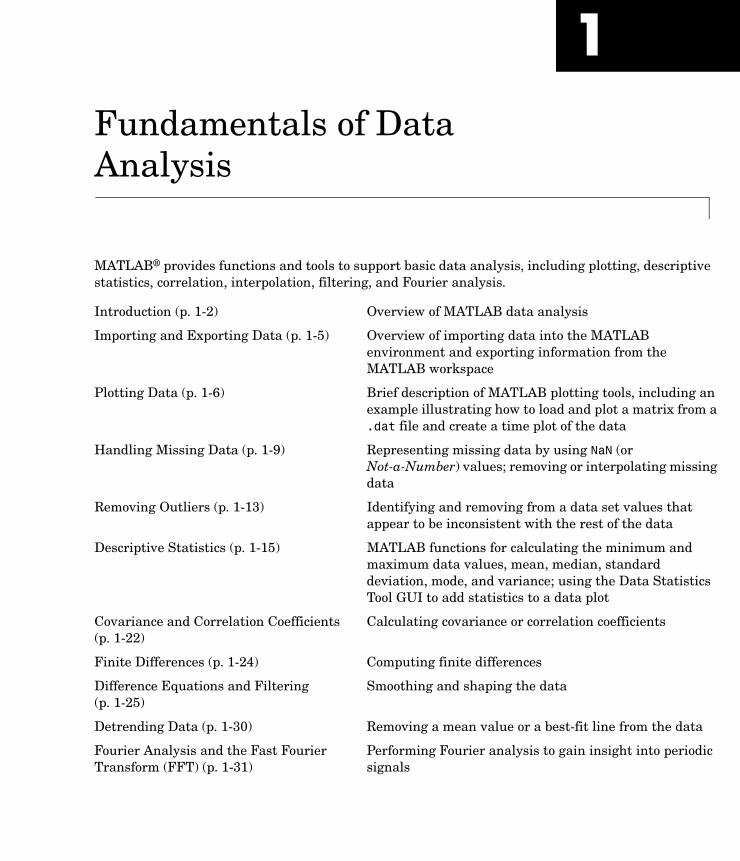
Fundamentals of Data AnalysisMATLAB® provides functions and tools to support basic data analysis, including plotting, descriptive statistics, correlation, interpolation, filtering, and Fourier analysis.
Introduction (p. 1-2) Overview of MATLAB data analysis
Importing and Exporting Data (p. 1-5) Overview of importing data into the MATLAB environment and exporting information from the MATLAB workspace
Plotting Data (p. 1-6) Brief description of MATLAB plotting tools, including an example illustrating how to load and plot a matrix from a .dat file and create a time plot of the data
Handling Missing Data (p. 1-9) Representing missing data by using NaN (or Not-a-Number) values; removing or interpolating missing data
Removing Outliers (p. 1-13) Identifying and removing from a data set values that appear to be inconsistent with the rest of the data
Descriptive Statistics (p. 1-15) MATLAB functions for calculating the minimum and maximum data values, mean, median, standard deviation, mode, and variance; using the Data Statistics Tool GUI to add statistics to a data plot
Covariance and Correlation Coefficients (p. 1-22)
Calculating covariance or correlation coefficients
Finite Differences (p. 1-24) Computing finite differences
Difference Equations and Filtering (p. 1-25)
Smoothing and shaping the data
Detrending Data (p. 1-30) Removing a mean value or a best-fit line from the data
Fourier Analysis and the Fast Fourier Transform (FFT) (p. 1-31)
Performing Fourier analysis to gain insight into periodic signals

1 Fundamentals of Data Analysis
1-2
IntroductionMATLAB® provides a number of functions for data analysis applications to compute descriptive statistics and correlation coefficients, interpolate and filter data, and perform Fourier analysis. You can also use the MATLAB Data Statistics tool to calculate and display descriptive statistics on a plot.
If you want to analyze time-series data, MATLAB provides the timeseries and tscollection objects that are specifically designed for handling time-indexed data. For more information about the time-series command-line API, see Chapter 3, “Analyzing Time Series from the Command Line.” Alternatively, you can use the Time Series Tools graphical user interface to facilitate time-series analysis and even generate M-code automatically. For more information, see Chapter 4, “Using the Time Series Tools GUI.”
MATLAB Data Analysis FunctionsThe basic MATLAB data analysis and statistics functions are located in the matlabroot/toolbox/matlab/datafun directory. To obtain detailed information about a function, use the syntax
help functionname
at the command line.
Note You can create your own data-analysis functions and add them as M-files to the matlabroot/toolbox/matlab/datafun directory. For more information, see the MATLAB Programming documentation.
Time-series and time-series collection functions are located in matlabroot/toolbox/matlab/timeseries and matlabroot/toolbox/matlab/tscollection, respectively. To obtain detailed information about a function, type
help timeseries/functioname
or
help tscollection/functioname
at the command line.

Introduction
Vector vs. Matrix Function ArgumentsWhereas some functions support only vector inputs, others accept matrices.
When your data set is a vector, it does not matter whether the vector is oriented in row or column direction.
When your data set contains multiple columns (i.e., is a matrix), the data analysis and statistics results are calculated independently for each column. This means, for example, that if you apply max to a matrix, the result is a row vector containing the maximum data values for each column.
MATLAB Tools for Data AnalysisFour MATLAB tools provide a graphical user interface to facilitate common data analysis tasks. The following table contains a brief description of each tool, as well as a reference to the relevant documentation where you can learn more.
Related ProductsThe table below lists the toolboxes that extend the basic data analysis and statistics functionality in MATLAB for specialized applications. For the latest
Tools for Data Analysis
Tool Description More Information
Plotting Graphing workspace variables and editing plot properties
MATLAB Graphics documentation
Data Statistics
Calculating and displaying descriptive statistics for a data set
“Using the Data Statistics Tool” on page 1-17
Basic Fitting
Basic data fitting with polynomial and spline models, and generating plots of fitted data and residuals
“Using the Basic Fitting Tool” on page 2-4
Time Series
Plotting and analyzing time-indexed data
Chapter 4, “Using the Time Series Tools GUI”
1-3

1 Fundamentals of Data Analysis
1-4
information about these and other MathWorks products, point your Web browser to
www.mathworks.com
Products That Extend MATLAB Data Analysis
Product Description
Bioinformatics Toolbox Read, analyze, and visualize genomic, proteomic, and microarray data
Curve Fitting Toolbox Perform model fitting and analysis
Financial Time Series Toolbox Analyze and manage financial time-series data
Financial Toolbox Analyze financial data and develop financial algorithms
Image Processing Toolbox Perform image processing, analysis, and algorithm development
Model-Based Calibration Toolbox
Calibrate complex powertrain systems
Neural Network Toolbox Design and simulate neural networks
Signal Processing Toolbox Perform signal processing, analysis, and algorithm development
Spline Toolbox Create and manipulate spline approximation models of data
Statistics Toolbox Apply statistical algorithms and probability models
System Identification Toolbox Create linear dynamic models from measured input-output data
Wavelet Toolbox Analyze and synthesize signals and images using wavelet techniques

Importing and Exporting Data
Importing and Exporting DataMATLAB provides a number of ways to import data from files or the clipboard into the workspace. For more information about importing various data formats, such as text, binary, or a standard format (such as HDF), see the MATLAB Programming documentation.
The easiest way to import data into MATLAB is to use the MATLAB Import Wizard. The Import Wizard processes your data source and recognizes data delimiters, as well as row or column headers, and extracts these headers.
When working with time-series data, you might want to use the Time Series Tools GUI to import the data. The Import Wizard in Time Series Tools facilitates assigning a time vector to the data during import. For more information, see “Importing Data into Time Series Tools” on page 4-9.
When you have finished analyzing your data, you might have created new variables. You can export the variables you created or updated during analysis to a variety of formats. For more information about exporting data from the MATLAB workspace, see the MATLAB Programming documentation.
1-5

1 Fundamentals of Data Analysis
1-6
Plotting DataAfter you import your data into MATLAB, it is a good idea to plot the data so that you can explore its features. If your data is a function of time, you can create a simple time plot with time as the independent variable on the x-axis.
An exploratory plot of your data enables you to identify discontinuities and potential outliers, as well as the regions of interest.
For more information about MATLAB plotting tools, see the MATLAB Graphics documentation.
To learn more about plotting time-series data in Time Series Tools, see Chapter 4, “Using the Time Series Tools GUI.”
Example — Loading and Plotting DataThis example illustrates how to load and plot data from a DAT file:
• “Loading the Data” on page 1-6
• “Plotting the Data” on page 1-7
Loading the DataImport the data by using the load command:
load count.dat
This creates the 24-by-3 matrix called count in the MATLAB workspace.
For more information about this data set, see “About the Example Data” on page 3-22.
Note By MATLAB convention, each row of a matrix is an observation, and each column is a variable.

Plotting Data
You can get the size of the data matrix by
[n,p] = size(count)n = 24p = 3
where n represents the number of rows, and p represents the number of columns.
Create a time vector, t, of integers from 1 to n:
t = 1:n;
Note For more information about working with time-indexed data, see “Example — Analyzing Time-Series Data at the Command Line” on page 3-22.
Plotting the DataUse the following commands to plot the data versus time and to annotate the plot:
set(0,'defaultaxeslinestyleorder','-|--|-.')set(0,'defaultaxescolororder',[0 0 0])plot(t,count), legend('Location 1','Location 2','Location 3',2)xlabel('Time'), ylabel('Vehicle Count'), grid on
1-7

1 Fundamentals of Data Analysis
1-8
The resulting plot shows the traffic counts at three locations over a 24-hour period.
0 5 10 15 20 250
50
100
150
200
250
300
Time
Veh
icle
Cou
nt
Location 1Location 2Location 3

Handling Missing Data
Handling Missing DataThe correct handling of missing data is a difficult problem in data analysis and often depends on your specific situation. Based on the context of your data, you must decide whether it is appropriate to exclude missing data from analysis or to replace the missing values, using a method such as interpolation.
This section contains the following topics:
• “Representing Missing Data Values” on page 1-9
• “Calculations with NaNs” on page 1-9
• “Removing NaNs from the Data” on page 1-10
• “Interpolating Missing Data” on page 1-11
Representing Missing Data ValuesIn MATLAB, missing or unavailable data values are represented by the special value NaN, which stands for Not-a-Number.
The IEEE floating-point arithmetic convention defines NaN as the result of an undefined operation, such as 0/0. However, NaN values are also convenient for calling out missing data.
Calculations with NaNsWhen you perform calculations on a MATLAB variable that contains NaNs, the NaN values are propagated to the final result.
For example, consider a matrix containing the 3-by-3 magic square with its center element set to NaN:
a = magic(3); a(2,2) = NaN a = 8 1 6 3 NaN 7 4 9 2
Compute a sum for each column in the matrix:
sum(a)
1-9

1 Fundamentals of Data Analysis
1-1
ans = 15 NaN 15
Note that the sum of the elements in the middle column is a NaN value because that column contains a NaN.
If you do not want to have NaNs in your final results, you must remove these values from your data. For more information, see “Removing NaNs from the Data” on page 1-10.
Note When you are working with time-series data in Time Series Tools, NaNs are ignored in calculations. When you are working with time-series objects at the command line, NaNs are ignored in calculations by default unless you modify the TreatNaNasMissing property. For more information, see “Properties of a timeseries Object” on page 3-5.
Removing NaNs from the DataYou can use isnan to remove NaNs from the data, as described in the following table.
Code Description
i = find(~isnan(x));x = x(i)
Find the indices of elements in a vector that are not NaNs. Keep only the non-NaN elements.
x = x(~isnan(x)); Remove NaNs from a vector x.
x(isnan(x)) = []; Remove NaNs from a vector x (alternative method).
X(any(isnan(X),2),:) = [];
Remove any rows containing NaNs from a matrix X.
0
Handling Missing Data
Note You must use the function isnan to find NaNs because, by IEEE arithmetic convention, the logical comparison NaN == NaN always produces 0 (i.e., it never evaluates to true). Therefore, you cannot use x(x==NaN) = [] to remove NaNs from your data.
If you frequently need to remove NaNs, you might want to write a short M-file function that you can call:
function X = excise(X)X(any(isnan(X),2),:) = [];
The following command computes the correlation coefficients of X after all rows containing NaNs are removed:
C = corrcoef(excise(X));
For more information about correlation coefficients, see “Correlation Coefficients” on page 1-23.
Interpolating Missing DataYou can use MATLAB interpolation to find intermediate points in your data. The simplest function for performing interpolation is the 1-D interpolation function interp1.
By default, the interpolation method is 'linear', which fits a straight line between a pair of existing data points to calculate the desired, nonexistent value. Other methods, which you can specify as arguments in the interp1 function, include
• 'nearest' — Nearest neighbor interpolation
• 'linear' — Linear interpolation
• 'spline' — Piecewise cubic spline interpolation
• 'pchip' or 'cubic' — Shape-preserving piecewise cubic interpolation
• 'v5cubic' — The cubic interpolation from MATLAB 5, which does not 'extrapolate' and uses 'spline' when X is not equally spaced
When you are working with timeseries and tscollection objects, only the linear and the zero-order hold ('zoh') interpolation methods are available. The
1-11

1 Fundamentals of Data Analysis
1-1
zero-order hold method “holds” the last existing data value constant until the next existing data value.
For more information about interp1, see the MATLAB documentation or type
help interp1
at the command line.
2
Removing Outliers
Removing OutliersWhen you visually examine a data plot, you might find that some points appear to be dramatically different from the rest of the data. In some cases, it is reasonable to consider such points outliers, or data values that have a low likelihood of being consistent with the rest of the data.
Removing an outlier has a greater effect on the standard deviation than on the mean of the data, because the standard deviation depends on the squares of the deviations. Deleting one such point will lead to a smaller standard deviation, and this might result in making other points appear as outliers! You should be cautious about changing data unless you are confident that you understand the source of the problem you want to correct.
Note When working with time-series objects, you can use the Time Series Tools GUI to remove outliers. For more information about selecting outliers by defining logical rules, see “Selecting Time-Series Data” on page 4-25.
The following example illustrates how to remove outliers from a data set. In this case, an outlier is defined to be a value that is at least three standard deviations away from the mean.
%% Import the sample dataload count.dat;
%% Calculate the mean and the standard deviationmu = mean(count)sigma = std(count)
MATLAB displays
mu =32.0000 46.5417 65.5833
sigma =25.3703 41.4057 68.0281
1-13
1 Fundamentals of Data Analysis
1-1
The number of outliers in each column of the count matrix is obtained with the following commands:
[n,p] = size(count)outliers = abs(count - mu(ones(n, 1),:)) > 3*sigma(ones(n, 1),:);nout = sum(outliers) % Calculate the number of outliers in each
% column
MATLAB displays
nout = 1 0 0
There is one outlier in the first column. To remove the entire row of data containing the outlier, type
count(any(outliers,2),:) = [];
4

Descriptive Statistics
Descriptive StatisticsMATLAB enables you to calculate the following descriptive statistics for your data:
• Maximum value
• Mean
• Median
• Minimum value
• Mode
• Standard deviation
• Variance
When your data set contains multiple columns, the descriptive statistics are calculated independently for each column.
This section contains the following topics:
• “Descriptive Statistics at the Command Line” on page 1-15
• “Using the Data Statistics Tool” on page 1-17
Descriptive Statistics at the Command LineYou can use the following MATLAB functions to calculate the descriptive statistics for your data.
Statistics Function Summary
Function Description
max Maximum value
mean Average or mean value
median Median value
min Smallest value
mode Most frequent value
1-15

1 Fundamentals of Data Analysis
1-1
The following examples illustrate how to apply MATLAB functions to calculate descriptive statistics:
• “Example 1 — Maximum, Minimum, and Standard Deviation” on page 1-16
• “Example 2 — Subtracting the Mean” on page 1-17
Example 1 — Maximum, Minimum, and Standard DeviationThe following example illustrates how to work with MATLAB statistics functions on a 24-by-3 matrix called count. For more information about this data, see “About the Example Data” on page 3-22.
load count.dat % Import the sample datamx = max(count)mu = mean(count)sigma = std(count)
MATLAB responds with
mx = 114 145 257
mu = 32.0000 46.5417 65.5833
sigma = 25.3703 41.4057 68.0281
You can locate the minimum and maximum data values in each matrix column by using a second output parameter indx, which outputs the index of a row. For example,
[mx,indx] = min(count)
std Standard deviation
var Variance of a vector (a measure of the spread or dispersion of the vector values)
Statistics Function Summary (Continued)
Function Description
6

Descriptive Statistics
produces the following results:
mx = 7 9 7
indx = 2 23 24
Here, the output variable mx is a row vector that contains the maximum value in each of the three data columns. The variable indx contains the row indices in each column that correspond to the maximum values.
To find the minimum value in the entire count matrix, you can reshape this 24-by-3 matrix into a 72-by-1 column vector by using the syntax count(:). Therefore, to find the smallest value in the entire count data set, you can use
min(count(:))
which produces
ans = 7
Example 2 — Subtracting the MeanYou can subtract the mean from each column of the data by using the following syntax:
[n,p] = size(count) % Get the size of the count matrixe = ones(n,1) % Define a vector of onesx = count - e*mu % Subtract the mean from each matrix element
Using the Data Statistics ToolThe MATLAB Data Statistics tool consists of a graphical user interface (GUI) that enables you to calculate and plot descriptive statistics along with the data.
Note The Data Statistics GUI is only available for 2-D plots.
In addition to the quantities listed in “Descriptive Statistics” on page 1-15, the Data Statistics tool calculates the range. The range is the interval between the
1-17

1 Fundamentals of Data Analysis
1-1
lowest value and the highest value in the data set. You cannot display the range on a plot.
This section contains the following topics:
• “Example — Calculating and Plotting Statistics” on page 1-18
• “Formatting Plots of Data Statistics” on page 1-19
• “Viewing Statistics for Multiple Data Sets” on page 1-20
• “Saving Statistics to the MATLAB Workspace” on page 1-21
Example — Calculating and Plotting Statistics
1 Plot your data. For example, use these commands to plot the historical population data from the United States census.
load censusplot(cdate,pop,'+')
2 In the figure window, select Tools > Data Statistics.
The Data Statistics tool calculates descriptive statistics for the X-data and the Y-data on the plot, and displays the results in the Data Statistics dialog.
Select the statistic you want to plot by clicking in its check box.
8

Descriptive Statistics
3 In the Data Statistics dialog, select the check box for each statistic you want to display on the plot.
For example, to plot the mean of the population (Y-data), select the check box for the Y mean. The plot legend is updated to include each statistic measure you display on the plot. For example, y mean.
Formatting Plots of Data StatisticsThe Data Statistics tool uses colors and line styles to distinguish statistics from the data on the plot. You can customize these plot properties.
Note Do not edit plot properties of data statistics until you finish adding them to the plot. If you add or remove statistics after editing plot properties, your changes will be lost.
To modify plot properties, enable plot editing and double-click the corresponding statistic on the plot. This opens the Property Editor, where you can modify the line object used to represent the statistic.
Plot of the mean of the population data.
The Data Statistics tool adds a legend automatically.
1-19

1 Fundamentals of Data Analysis
1-2
Alternatively, enable plot editing, right-click the statistic on the plot, and select an option from the shortcut menu. For example, you can modify the line width, line style, or color.
Viewing Statistics for Multiple Data SetsThe Data Statistics tool calculates basic statistics for every 2-D plot in a graph but displays the statistics for only one data set at time.
To view the statistics for a particular data set, select it from the Statistics for list, as shown below.
The Statistics for list includes all the data sets you plotted on the graph, identified by a default or a user-defined tag. Default tag names are generated as follows: data1 to identify the first plot, data2 to identify the second plot, and so on.
Lists the data sets on which the statistics have been calculated
0

Descriptive Statistics
Saving Statistics to the MATLAB WorkspaceTo save the statistics generated by the Data Statistics tool to the MATLAB workspace, follow this procedure.
Note When your plot contains multiple data sets, you must repeat this procedure for each data set.
1 Click the Save to Workspace button.
2 In the Save Statistics to Workspace dialog, specify the sets of statistics you want to save (X-data and Y-data). Enter the corresponding variable names.
The Data Statistics tool saves each set of statistics to a structure. For example, when you select to save the X-data statistics for the census data in the variable census_dates, the resulting structure looks like this:
census_dates =
min: 1790 max: 1990 mean: 1890 median: 1890 std: 62.0484 range: 200
Specify the set of statistics you want to save.
Assign a name to the variable.
1-21
1 Fundamentals of Data Analysis
1-2
Covariance and Correlation CoefficientsMATLAB provides the following two functions for computing covariance and correlation coefficients.
Covariancecov calculates the covariance matrix. For the special case when a vector is the argument, cov returns the variance.
The covariance matrix has the following properties:
• diag(cov(X)) is a vector of variances for each column, which represent a measure of the spread or dispersion of the values in a column.
• sqrt(diag(cov(X))) is a vector of standard deviations.
• The off-diagonal elements of the covariance matrix represent the covariance between the individual data columns.
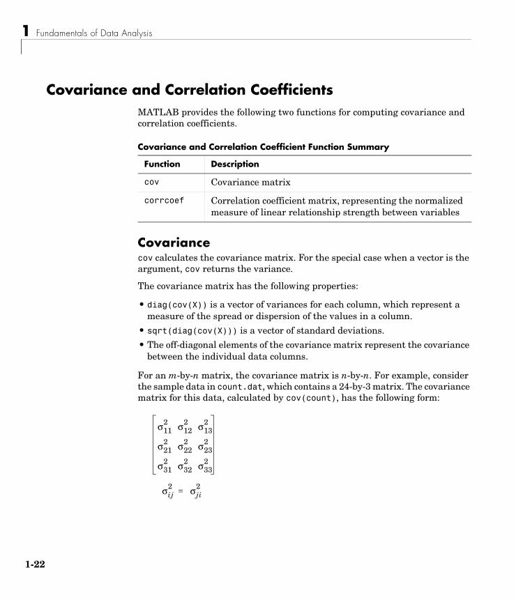
For an m-by-n matrix, the covariance matrix is n-by-n. For example, consider the sample data in count.dat, which contains a 24-by-3 matrix. The covariance matrix for this data, calculated by cov(count), has the following form:
Covariance and Correlation Coefficient Function Summary
Function Description
cov Covariance matrix
corrcoef Correlation coefficient matrix, representing the normalized measure of linear relationship strength between variables
σ112 σ12
2 σ132
σ212 σ22
2 σ232
σ312 σ32
2 σ332
σij2 σji
2=
2
Covariance and Correlation Coefficients
Here, is the covariance between column i and column j of the data. Because the count matrix contains three columns, the covariance matrix is 3-by-3.
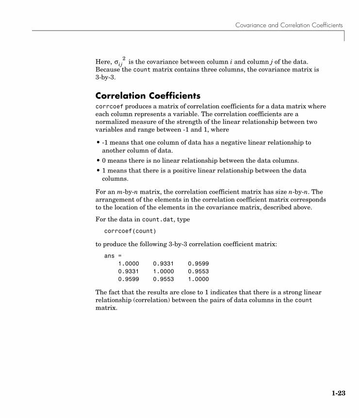
Correlation Coefficientscorrcoef produces a matrix of correlation coefficients for a data matrix where each column represents a variable. The correlation coefficients are a normalized measure of the strength of the linear relationship between two variables and range between -1 and 1, where
• -1 means that one column of data has a negative linear relationship to another column of data.
• 0 means there is no linear relationship between the data columns.
• 1 means that there is a positive linear relationship between the data columns.
For an m-by-n matrix, the correlation coefficient matrix has size n-by-n. The arrangement of the elements in the correlation coefficient matrix corresponds to the location of the elements in the covariance matrix, described above.
For the data in count.dat, type
corrcoef(count)
to produce the following 3-by-3 correlation coefficient matrix:
ans = 1.0000 0.9331 0.9599 0.9331 1.0000 0.9553 0.9599 0.9553 1.0000
The fact that the results are close to 1 indicates that there is a strong linear relationship (correlation) between the pairs of data columns in the count matrix.
σij2
1-23

1 Fundamentals of Data Analysis
1-2
Finite DifferencesMATLAB provides three functions for finite difference calculations.
The diff function computes the difference between successive elements in a numeric vector. That is, diff(X) is [X(2)-X(1) X(3)-X(2)... X(n)-X(n-1)].
For a vector A,
A = [9 -2 3 0 1 5 4];diff(A)
ans = -11 5 -3 1 4 -1
Besides computing the first difference, you can use diff to determine certain characteristics of vectors. For example, you can use diff to determine whether the vector values are monotonically increasing or decreasing, or whether a vector has equally spaced elements.
The following table provides examples for using diff with a vector x.
Function Description
del2 Discrete Laplacian of a matrix
diff Differences between successive elements of a vector; numerical partial derivatives of a vector
gradient Numerical partial derivatives of a matrix
Test Description
any(diff(x)==0) Tests whether there are any repeated elements in X
all(diff(x)>0) Tests whether the values are monotonically increasing
all(diff(diff(x))==0) Tests for equally spaced vector elements
4
Difference Equations and Filtering
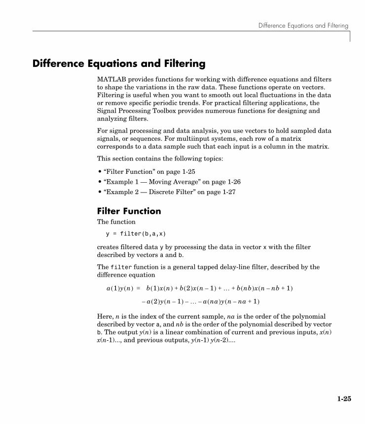
Difference Equations and FilteringMATLAB provides functions for working with difference equations and filters to shape the variations in the raw data. These functions operate on vectors. Filtering is useful when you want to smooth out local fluctuations in the data or remove specific periodic trends. For practical filtering applications, the Signal Processing Toolbox provides numerous functions for designing and analyzing filters.
For signal processing and data analysis, you use vectors to hold sampled data signals, or sequences. For multiinput systems, each row of a matrix corresponds to a data sample such that each input is a column in the matrix.
This section contains the following topics:
• “Filter Function” on page 1-25
• “Example 1 — Moving Average” on page 1-26
• “Example 2 — Discrete Filter” on page 1-27
Filter FunctionThe function
y = filter(b,a,x)
creates filtered data y by processing the data in vector x with the filter described by vectors a and b.
The filter function is a general tapped delay-line filter, described by the difference equation
Here, n is the index of the current sample, na is the order of the polynomial described by vector a, and nb is the order of the polynomial described by vector b. The output y(n) is a linear combination of current and previous inputs, x(n) x(n-1)..., and previous outputs, y(n-1) y(n-2)....
a 1( )y n( ) b 1( )x n( ) b 2( )x n 1–( ) … b nb( )x n nb– 1+( )+ + +=
a 2( )y n 1–( )– …– a na( )y n na– 1+( )–
1-25

1 Fundamentals of Data Analysis
1-2
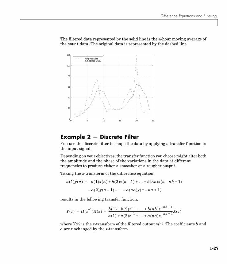
Example 1 — Moving AverageThe process for smoothing the data in count.dat with a moving average filter to see the average traffic flow over a 4-hour window — covering the current hour and the previous three hours — can be represented by the difference equation
The corresponding vectors are
a = 1;b = [1/4 1/4 1/4 1/4];
Note Enter the format command format rat to display and enter data using the rational format.
Executing the command
load count.dat
creates the matrix count in the workspace.
Extract the first column of counts and assign it to the vector x:
x = count(:,1);
The 4-hour moving average of the data is calculated by using
y = filter(b,a,x);
Compare the original data and the smoothed data with an overlaid plot of the two curves:
t = 1:length(x);plot(t,x,'-.',t,y,'-'), grid onlegend('Original Data','Smoothed Data',2)
y n( ) 14---x n( ) 1
4---x n 1–( ) 1
4---x n 2–( ) 1
4---x n 3–( )+ + +=
6
Difference Equations and Filtering
The filtered data represented by the solid line is the 4-hour moving average of the count data. The original data is represented by the dashed line.
Example 2 — Discrete FilterYou use the discrete filter to shape the data by applying a transfer function to the input signal.
Depending on your objectives, the transfer function you choose might alter both the amplitude and the phase of the variations in the data at different frequencies to produce either a smoother or a rougher output.
Taking the z-transform of the difference equation
results in the following transfer function:
where Y(z) is the z-transform of the filtered output y(n). The coefficients b and a are unchanged by the z-transform.
0 5 10 15 20 250
20
40
60
80
100
120
Original DataSmoothed Data
a 1( )y n( ) b 1( )x n( ) b 2( )x n 1–( ) … b nb( )x n nb– 1+( )+ + +=
a 2( )y n 1–( )– …– a na( )y n na– 1+( )–
Y z( ) H z 1–( )X z( ) b 1( ) b 2( )z 1– … b nb( )z nb– 1++ + +
a 1( ) a 2( )z 1– … a na( )z na– 1++ + +----------------------------------------------------------------------------------------------X z( )= =
1-27
1 Fundamentals of Data Analysis
1-2
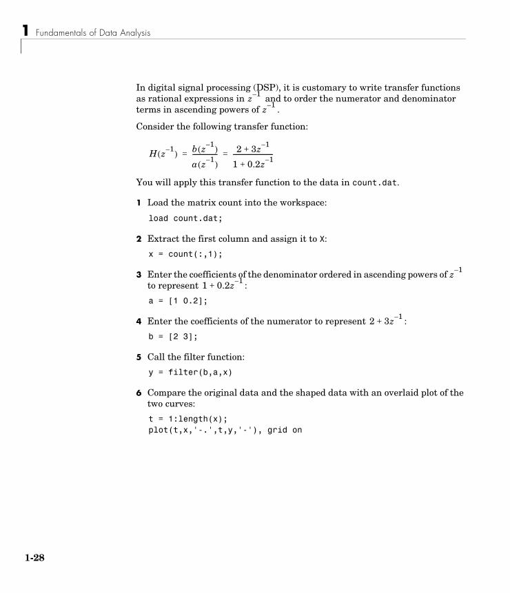
In digital signal processing (DSP), it is customary to write transfer functions as rational expressions in and to order the numerator and denominator terms in ascending powers of .
Consider the following transfer function:
You will apply this transfer function to the data in count.dat.
1 Load the matrix count into the workspace:
load count.dat;
2 Extract the first column and assign it to X:
x = count(:,1);
3 Enter the coefficients of the denominator ordered in ascending powers of to represent :
a = [1 0.2];
4 Enter the coefficients of the numerator to represent :
b = [2 3];
5 Call the filter function:
y = filter(b,a,x)
6 Compare the original data and the shaped data with an overlaid plot of the two curves:
t = 1:length(x);plot(t,x,'-.',t,y,'-'), grid on
z 1–
z 1–
H z 1–( ) b z 1–( )
a z 1–( )---------------- 2 3z 1–+
1 0.2z 1–+--------------------------= =
z 1–
1 0.2z 1–+
2 3z 1–+
8

Difference Equations and Filtering
legend('Original Data','Shaped Data',2)
This filter primarily modified the amplitude of the original data.
1-29
1 Fundamentals of Data Analysis
1-3
Detrending Datadetrend removes a constant or linear trend from your data. If your data contains several data columns, each data column is detrended separately.
You decide whether it makes sense to remove trend effects in the data based on the objectives of your analysis.
For example, you might want to detrend data when analyzing
• Local fluctuations in the data, rather than focusing on systematic variations in the mean.
• Evolution of a time series in time, as described by the autocorrelation function. For more information, see “Correlation Coefficients” on page 1-23.
0

Fourier Analysis and the Fast Fourier Transform (FFT)
Fourier Analysis and the Fast Fourier Transform (FFT)Fourier analysis is extremely useful for data analysis, as it breaks down a signal into constituent sinusoids of different frequencies. For sampled vector data, Fourier analysis is performed using the discrete Fourier transform (DFT).
The fast Fourier transform (FFT) is an efficient algorithm for computing the DFT of a sequence; it is not a separate transform. It is particularly useful in areas such as signal and image processing, filtering, convolution, frequency analysis, and power spectrum estimation.
This section contains the following topics:
• “Function Summary” on page 1-31
• “Calculating the FFT” on page 1-32
• “Magnitude and Phase of Transformed Data” on page 1-36
• “FFT Length vs. Performance” on page 1-38
Function SummaryMATLAB provides a collection of functions for computing and working with Fourier transforms.
FFT Function Summary
Function Description
abs Absolute value and complex magnitude
angle Phase angle
cplxpair Sort numbers into complex conjugate pairs
fft One-dimensional discrete Fourier transform
fft2 Two-dimensional discrete Fourier transform
fftn N-dimensional discrete Fourier transform
fftshift Shift DC component of discrete Fourier transform to center of spectrum
1-31

1 Fundamentals of Data Analysis
1-3
Calculating the FFTConsider an input sequence x with length N input sequence. The FFT is given by the vector X of length N.
fft (vector X) and ifft (vector x) implement the following relationships, respectively:
Note Because the first element of a MATLAB vector has an index 1, the summations in the above equations are from 1 to N. These produce results that are identical to the traditional Fourier equations with summations from 0 to N-1.
If x(n) is real, you can rewrite the above equation in terms of a summation of sine and cosine functions with real coefficients:
ifft Inverse one-dimensional discrete Fourier transform
ifft2 Inverse two-dimensional discrete Fourier transform
nextpow2 Next higher power of two
ifftn Inverse N-dimensional discrete Fourier transform
unwrap Unwrap phase angle in radians
FFT Function Summary (Continued)
Function Description
X k( ) x n( )ej2π k 1–( ) n 1–
N-------------⎝ ⎠⎛ ⎞ 1 k N≤ ≤–
n 1=
N
∑=
x n( ) 1N---- X k( )e
j2π k 1–( ) n 1–N
-------------⎝ ⎠⎛ ⎞ 1 n N≤ ≤
k 1=
N
∑=
2

Fourier Analysis and the Fast Fourier Transform (FFT)
where
Example — Calculating the FFT of a Column VectorConsider the following column vector:
x = [4 3 7 -9 1 0 0 0]' ;
The FFT of x is found by using
y = fft(x)
which results in
y =6.000011.4853 - 2.7574i-2.0000 -12.0000i-5.4853 +11.2426i18.0000-5.4853 -11.2426i-2.0000 +12.0000i11.4853 + 2.7574i
Notice that although the sequence x is real, y is complex. The first component of the transformed data is the constant contribution and the fifth element corresponds to the Nyquist frequency. The last three values of y correspond to negative frequencies and, for the real sequence x, they are complex conjugates of three components in the first half of y.
Example — Using FFT to Calculate Sunspot Periodicity Suppose you want to analyze the variations in sunspot activity over the last 300 years. This example illustrates the cyclical nature of sunspot activity, which reaches a maximum about every 11 years.
Astronomers have tabulated a quantity called the Wolfer number for almost 300 years. This quantity measures both the number and the size of sunspots.
x n( ) 1N---- a k( ) 2π k 1–( ) n 1–( )
N-------------------------------------------⎝ ⎠⎛ ⎞cos b k( ) 2π k 1–( ) n 1–( )
N-------------------------------------------⎝ ⎠⎛ ⎞sin+
k 1=
N
∑=
a k( ) X k( )( ), b k( )real X k( )( ), 1 n N≤ ≤imag–= =
1-33

1 Fundamentals of Data Analysis
1-3
Load and plot the sunspot data:
load sunspot.datyear = sunspot(:,1);wolfer = sunspot(:,2);plot(year,wolfer)title('Sunspot Data')
Now take the FFT of the sunspot data:
Y = fft(wolfer);
The result of this transform is the complex vector Y. The magnitude of Y squared is called the estimated power spectrum. A plot of the estimated power spectrum versus frequency is called a periodogram.
1700 1750 1800 1850 1900 1950 20000
20
40
60
80
100
120
140
160
180
200Sunspot Data
4

Fourier Analysis and the Fast Fourier Transform (FFT)
Remove the first component of Y, which is simply the sum of the data, and plot the results:
N = length(Y);Y(1) = [];power = abs(Y(1:N/2)).^2;nyquist = 1/2;freq = (1:N/2)/(N/2)*nyquist;plot(freq,power), grid onxlabel('cycles/year')title('Periodogram')
The scale in cycles/year is somewhat inconvenient. You can plot in years/cycle and estimate what one cycle is. For convenience, plot the power versus period (where period = 1./freq) from 0 to 40 years/cycle:
period = 1./freq;plot(period,power), axis([0 40 0 2e7]), grid onylabel('Power')xlabel('Period(Years/Cycle)')
0 0.05 0.1 0.15 0.2 0.25 0.3 0.35 0.4 0.45 0.50
0.2
0.4
0.6
0.8
1
1.2
1.4
1.6
1.8
2x 10
7
cycles/year
Periodogram
1-35

1 Fundamentals of Data Analysis
1-3
In order to determine the cycle more precisely,
[mp,index] = max(power);period(index)
ans = 11.0769
This plot confirms the cyclical nature of sunspot activity, which reaches a maximum about every 11 years.
Magnitude and Phase of Transformed Data Important information about a transformed sequence includes its magnitude and phase. The MATLAB functions abs and angle calculate this information.
To try this, create a time vector t, and use this vector to create a sequence x consisting of two sinusoids at different frequencies:
t = 0:1/100:10-1/100;x = sin(2*pi*15*t) + sin(2*pi*40*t);
Now use the fft function to compute the DFT of the sequence. The code below calculates the magnitude and phase of the transformed sequence. It uses the
0 5 10 15 20 25 30 35 400
0.2
0.4
0.6
0.8
1
1.2
1.4
1.6
1.8
2x 10
7
Period(Years/Cycle)
Pow
er
6
Fourier Analysis and the Fast Fourier Transform (FFT)
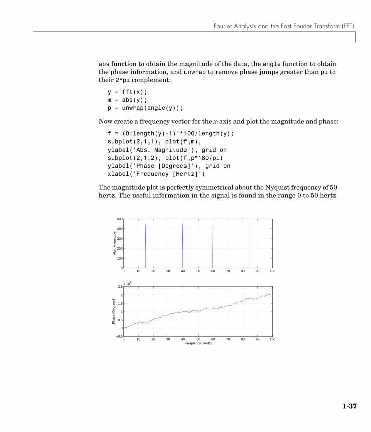
abs function to obtain the magnitude of the data, the angle function to obtain the phase information, and unwrap to remove phase jumps greater than pi to their 2*pi complement:
y = fft(x); m = abs(y);p = unwrap(angle(y));
Now create a frequency vector for the x-axis and plot the magnitude and phase:
f = (0:length(y)-1)'*100/length(y);subplot(2,1,1), plot(f,m), ylabel('Abs. Magnitude'), grid onsubplot(2,1,2), plot(f,p*180/pi)ylabel('Phase [Degrees]'), grid onxlabel('Frequency [Hertz]')
The magnitude plot is perfectly symmetrical about the Nyquist frequency of 50 hertz. The useful information in the signal is found in the range 0 to 50 hertz.
0 10 20 30 40 50 60 70 80 90 1000
100
200
300
400
500
Abs
. Mag
nitu
de
0 10 20 30 40 50 60 70 80 90 100−0.5
0
0.5
1
1.5
2
2.5x 10
4
Pha
se [D
egre
es]
Frequency [Hertz]
1-37

1 Fundamentals of Data Analysis
1-3
FFT Length vs. PerformanceThe execution time for the fft depends on the length of the transform.
You can add a second argument to fft to specify a number of points n for the transform:
y = fft(x,n)
With this syntax, fft pads x with zeros if it is shorter than n, or truncates it if it is longer than n. If you do not specify n, fft defaults to the length of the input sequence. fft is fastest for powers of two. It is almost as fast for lengths that have only small prime factors. It is typically several times slower for lengths that are prime or have large prime factors.
The inverse FFT function ifft also accepts a transform length argument.
8

2
Data Fitting Using Linear RegressionMATLAB enables you to apply linear regression to model the relationship between dependent and independent variables by using the MATLAB Basic Fitting tool, or by working at the MATLAB command line.
Introduction (p. 2-2) Overview of MATLAB data fitting; brief description of the Curve Fitting Toolbox, which extends the MATLAB functionality
Using the Basic Fitting Tool (p. 2-4) Describes the Basic Fitting tool GUI for fitting polynomial and spline models, generating plots of fitted data and residuals, and saving fit information to the workspace; example illustrates how to work with the Basic Fitting tool
Data Fitting at the Command Line (p. 2-17)
Fitting polynomials, more general linear models, and multiple regression models by using MATLAB functions; generating plots of fitted data and residuals
Example — Fitting Data at the Command Line (p. 2-23)
Illustrates how to use MATLAB functions to fit polynomials, generate plots of fitted data and residuals, and calculate confidence bounds
2 Data Fitting Using Linear Regression
2-2
IntroductionMATLAB enables you to perform basic data fitting by using linear regression to model your data. A model is a relationship between independent and dependent variables.
To model your data, you can either use the MATLAB Basic Fitting tool or issue commands in the MATLAB Command Window.
You can use MATLAB to fit nonlinear data if you first transform it in a variable that makes the model linear.
In this chapter, you learn how to
• Generate a simple fit
• Plot the fit on top of the data
• Evaluate the goodness of fit by examining a plot of the residuals
For an example of fitting data by using the Basic Fitting tool, see “Example — Using the MATLAB Basic Fitting Tool” on page 2-9. For a demonstration of data fitting from the MATLAB Command Window, see “Example — Fitting Data at the Command Line” on page 2-23.
When to Use the Curve Fitting ToolboxFor advanced curve-fitting capabilities, use the Curve Fitting Toolbox, which extends the basic MATLAB functionality by enabling
• Nonlinear parametric fitting, including standard linear least squares, nonlinear least squares, weighted least squares, constrained least squares, and robust fitting procedures
• Nonparametric fitting
• Built-in statistics for determining the goodness of fit
• GUI that facilitates data sectioning and smoothing
• Extrapolation, differentiation, and integration
• Saving fit results in various formats, including M-files, binary files, and workspace variables

Introduction
Residuals and the Goodness of FitThe residuals are defined as the difference between the observed values of the dependent variable and the values of the dependent variable that are predicted by the model. When you fit a good model to your data, the residuals approximate random errors.
When MATLAB calculates fit parameters, it minimizes the sum of the squares of the residuals — a least-squares fit.
You can gain insight into the “goodness” of a fit by visually examining a plot of the residuals: residuals behaving randomly suggest that the model fits the data well, and residuals displaying a pattern indicate a poor fit.
Note that the “goodness” of a fit must be determined in the context of your data. For example, if your goal of fitting the data is to extract coefficients that have a physical meaning, then it is important that your model reflect the physics of the data. In this case, understanding what your data represents and how it was measured is just as important as evaluating the goodness of fit.
2-3
2 Data Fitting Using Linear Regression
2-4
Using the Basic Fitting ToolThis section contains the following topics:
• “What Is the Basic Fitting GUI?” on page 2-4
• “Sorting Large Data Sets to Improve Performance” on page 2-5
• “Basic Fitting Options” on page 2-5
• “Example — Using the MATLAB Basic Fitting Tool” on page 2-9
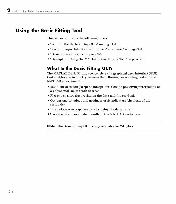
What Is the Basic Fitting GUI?The MATLAB Basic Fitting tool consists of a graphical user interface (GUI) that enables you to quickly perform the following curve-fitting tasks in the MATLAB environment:
• Model the data using a spline interpolant, a shape-preserving interpolant, or a polynomial (up to tenth degree)
• Plot one or more fits overlaying the data and the residuals
• Get parameter values and goodness-of-fit indicators (the norm of the residuals)
• Interpolate or extrapolate data by using the data model
• Save the fit and evaluated results to the MATLAB workspace
Note The Basic Fitting GUI is only available for 2-D plots.

Using the Basic Fitting Tool
Sorting Large Data Sets to Improve PerformanceIf your data set is large and the values are not sorted in ascending order, it might take some time to fit your data. This can occur because the Basic Fitting tool sorts the values first. In some cases, you can speed up the fitting process by presorting the data before you open the Basic Fitting tool.
For example, use the following syntax at the command line to create sorted vectors, x_sorted and y_sorted, from the original data vectors x and y:
[x_sorted, i] = sort(x);y_sorted = y(i);
Basic Fitting OptionsYou open the Basic Fitting tool from a MATLAB figure window where you plotted the data by selecting Tools > Basic Fitting.
The Basic Fitting GUI, shown below, contains the following categories of options:
• “Select Data” on page 2-6 — Enable you to select the data that you want to fit from a list of data sets currently plotted in the figure window
• “Plot Fits” on page 2-7 — Enable adding one or more fits to the plot, displaying equations, and calculating and plotting residuals
• “Numerical Results” on page 2-8 — Display the parameters for a specific fit
• “Find Y = f(X)” on page 2-8 — Interpolate or extrapolate ordinate values by using the selected fit
Note To expand the Basic Fitting dialog to display all options, click the button in the lower right corner.
2-5

2 Data Fitting Using Linear Regression
2-6
Select DataFrom the list, select the data you want to fit from a list of data sets you plotted in the figure window.
You can only fit one data set at a time. However, you can generate and display multiple fits for a selected data set. Use the Property Editor to edit the name of a data set.
Center and Scale X DataSelect this check box when MATLAB displays the following warning message:
Polynomial is badly conditioned. Removing repeated data points or centering and scaling may improve results.
This warning is displayed when the X (independent data) values are large and the degree of the selected polynomial is high enough to generate numbers with dramatically different orders of magnitude in the Vandermonde matrix, which is constructed during the fitting procedure to compute estimates of the

Using the Basic Fitting Tool
polynomial parameters. Because one column of the Vandermonde matrix always contains 1’s, and because powers of large X values can be orders of magnitude larger than 1, the precision of the parameter estimates suffers.
To improve the precision of the computed parameters, the columns of the Vandermonde matrix can be brought to the same order of magnitude by centering the X data at zero mean and scaling the data to a unit standard deviation:
NewXData=(XData-mean(XData))./std(XData)
Plot FitsThis pane contains options for adding one or more fits to the plot, displaying equations, and calculating and plotting residuals.
• Check to display fits on figure — Select to display one or more fits in the figure window for the selected data set:
- spline interpolant — Uses the spline function
- shape-preserving interpolant — Uses the pchip function
- linear, quadratic, cubic, 4th,..., 10th degree polynomial — Uses the polyfit function
Note Use the lowest degree polynomial that gives a good fit. When fitting N points, if you select a polynomial of degree higher than (N-1), the system becomes underdetermined, and the extraneous coefficients are set to 0 during the calculation.
• Show equations — Select this check box to display the fit equation on the plot.
Significant digits — Select the number of significant digits for the coefficients of the displayed equation.
• Plot residuals — Select to plot residuals, where each residual is the difference between an ordinate data value and a corresponding fit value at a specific abscissa value.
Select the type of residual plot: Bar plot, Scatter plot, or Line plot.
2-7

2 Data Fitting Using Linear Regression
2-8
Select where to plot the residuals:
- Subplot — Plot residuals in the same figure window as the data
- Separate figure — Plot residuals in a new figure window
Note When you use subplots to plot several data sets, you can only plot residuals in a separate window.
- Show norm of residuals — Select this check box to display the norm of the residuals, calculated by using the norm function, norm(V,2), where V is the vector of residuals. The higher the degree of the polynomial, the lower the norm. A smaller norm indicates a better fit than a larger one.
Numerical ResultsThis pane displays the numerical results of a specific fit. It is not necessary to display this fit on the figure (by selecting it in the Plot Fits pane) in order to view the numerical results of the fit.
• Fit — Select the type of fit for which you want to display the numerical results. If the selected fit is not currently displayed in the figure window, select the corresponding check box in the Plot fits pane. When you first open the Numerical Results pane, the results of the last fit you selected in Plot fits are displayed.
• Save to workspace — Click to open the dialog where you specify how to save the fit parameters and norm of the residuals to workspace variables.
Find Y = f(X)In this pane, you can interpolate or extrapolate ordinate values by using the selected Fit.
• Enter value(s) — Enter one or more X values (or specify a valid MATLAB expression) at which you want to evaluate the ordinate value f(X) by using the selected Fit. For example, you can specify X as 1:2:10 or [10 15]. Then click Evaluate.
• Save to workspace — Available only after you evaluate interpolated or extrapolated points using the fit. Click to open the dialog where you can save the evaluated results to the workspace.

Using the Basic Fitting Tool
• Plot evaluated results — Select this check box to display the evaluated points on the plot.
Example — Using the MATLAB Basic Fitting ToolThis example illustrates how to use the Basic Fitting tool in MATLAB by fitting a cubic polynomial to the census data:
• “Graphically Fitting the Data” on page 2-9
• “Fit Parameters and the Goodness of Fit” on page 2-13
• “Predicting the U.S. Population by Using the Fit” on page 2-14
Graphically Fitting the DataTo open the Basic Fitting dialog,
1 Load and plot the census data:
load censusplot(cdate,pop,'ro')
The file census.mat contains U.S. population data for the years 1790 through 1990.
2-9

2 Data Fitting Using Linear Regression
2-1
2 Open the Basic Fitting dialog by selecting Tools > Basic Fitting in the figure window.
3 In the Basic Fitting dialog, select the cubic check box to fit a cubic polynomial to the data.
MATLAB displays the following warning:
Polynomial is badly conditioned. Removing repeated data points or centering and scaling may improve results.
To fix the problem, select the Center and scale X data check box. For more information about this option, see “Center and Scale X Data” on page 2-6.
0

Using the Basic Fitting Tool
Note The values of the fitted coefficients are different after centering and scaling the independent variable when compared to the values obtained from the original data. However, this does not change the functional form of the data and the resulting goodness of fit statistics. Therefore, the fitted plot shows the original, unscaled X-data values.
4 In the Basic Fitting dialog, specify to
- Display the fit equation in the plot
- Plot the fit residuals as a bar plot or a subplot in the figure window that contains the data
- Display the norm of the residuals
Fit a cubic polynomial to the data.
Show the equation.
Show the norm of the residuals.
Plot the residuals as a bar plot in the data figure window.
Current data set
2-11

2 Data Fitting Using Linear Regression
2-1
The resulting fit and residuals are shown in the following plot:
The legend contains the name of the data set and the fit equation. If the legend covers part of the plot, click and drag it to another location.
For comparison, try fitting another equation to the census data by selecting the corresponding Plot fit check box in the Basic Fitting dialog. The plot legend is automatically updated when you add or remove data sets or fits. When you finish adding information to the plot, you can change the default plot settings by using the Property Editor. These changes are undone when you perform another fit.
Note If you change the name of a data set in the plot legend, the corresponding name is automatically updated in the Select Data list of the Basic Fitting dialog.
Click and drag legend if it covers part of the plot.
2

Using the Basic Fitting Tool
Fit Parameters and the Goodness of FitIn the Basic Fitting dialog, click the button to display the estimated parameters and the norm of the residuals, which indicates the goodness of fit.
To explore the results of a specific fit, select the type of fit from the Fit list.
Note If you also want to display this fit on the plot, you must select the corresponding Plot fits check box.
2-13
2 Data Fitting Using Linear Regression
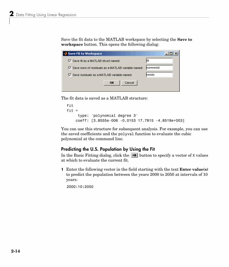
2-1
Save the fit data to the MATLAB workspace by selecting the Save to workspace button. This opens the following dialog:
The fit data is saved as a MATLAB structure:
fitfit = type: 'polynomial degree 3' coeff: [3.8555e-006 -0.0153 17.7815 -4.8519e+003]
You can use this structure for subsequent analysis. For example, you can use the saved coefficients and the polyval function to evaluate the cubic polynomial at the command line.
Predicting the U.S. Population by Using the FitIn the Basic Fitting dialog, click the button to specify a vector of X values at which to evaluate the current fit.
1 Enter the following vector in the field starting with the text Enter value(s) to predict the population between the years 2000 to 2050 at intervals of 10 years:
2000:10:2050
4

Using the Basic Fitting Tool
2 Click Evaluate.
The X-values and the corresponding values for f(X) are evaluated from the fit and displayed, as shown below.
2-15

2 Data Fitting Using Linear Regression
2-1
3 Select the Plot evaluated results check box to display the evaluated points with the data set in the plot, as shown in the following figure:
4 Save the extrapolated data to the MATLAB workspace by clicking Save to workspace. This opens the following dialog, where you specify the variable names:
6
Data Fitting at the Command Line
Data Fitting at the Command LineThis section contains the following topics:
• “Polynomial Model” on page 2-17
• “Linear Model with Nonpolynomial Terms” on page 2-19
• “Multiple Regression” on page 2-21
Polynomial ModelMATLAB provides two functions for modeling your data by using a polynomial function.
Suppose you measure a quantity y at several values of time t:
t = [0 .3 .8 1.1 1.6 2.3]';y = [0.5 0.82 1.14 1.25 1.35 1.40]';plot(t,y,'o'), grid on
Polynomial Fit Functions
Function Description
polyfit polyfit(x,y,n) finds the coefficients of a polynomial p(x) of degree n that fits the data y by minimizing the sum of the squares of the deviations of the data from the model (least-squares fit).
polyval polyval(p,x) returns the value of a polynomial of degree n, determined by polyfit, evaluated at x.
2-17

2 Data Fitting Using Linear Regression
2-1
Based on the plot, it is possible that the data can be modeled by a polynomial function
The unknown coefficients a0, a1, and a2 are computed by minimizing the sum of the squares of the deviations of the data from the model (least-squares fit).
To find the polynomial coefficients, type
p=polyfit(t,y,2)
at the command line.
MATLAB calculates the polynomial coefficients in descending powers:
p = -0.2387 0.9191 0.5318
The second-order polynomial model of the data is given by
To see how good the fit is, evaluate the polynomial at uniformly spaced times t2 and overlay the original data on a plot:
y a2t2 a1t a+ + 0=
y 0.2387t2– 0.9191t 0.5318+ +=
8
Data Fitting at the Command Line
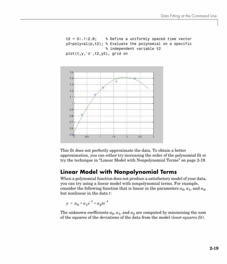
t2 = 0:.1:2.8; % Define a uniformly spaced time vectory2=polyval(p,t2); % Evaluate the polynomial on a specific
% independent variable t2plot(t,y,'o',t2,y2), grid on
This fit does not perfectly approximate the data. To obtain a better approximation, you can either try increasing the order of the polynomial fit or try the technique in “Linear Model with Nonpolynomial Terms” on page 2-19.
Linear Model with Nonpolynomial TermsWhen a polynomial function does not produce a satisfactory model of your data, you can try using a linear model with nonpolynomial terms. For example, consider the following function that is linear in the parameters a0, a1, and a2, but nonlinear in the data t:
The unknown coefficients a0, a1, and a2 are computed by minimizing the sum of the squares of the deviations of the data from the model (least-squares fit).
y a0 a1e t– a2te t–+ +=
2-19

2 Data Fitting Using Linear Regression
2-2
Construct and solve the set of simultaneous equations by forming the Vandermonde matrix, X, and solving for the parameters by using the backslash operator:
X = [ones(size(t)) exp(-t) t.*exp(-t)];a = X\y
a = 1.3974- 0.8988
0.4097
The model of the data is given by
Now evaluate the model at regularly spaced points and plot the model with the original data, as follows:
T = (0:0.1:2.5)';Y = [ones(size(T)) exp(-T) T.*exp(-T)]*a;plot(T,Y,'-',t,y,'o'), grid on
In this case, the fitted curve appears to go through each data point and, therefore, appears to be a much better fit than the second-order polynomial.
y 1.3974 0.8988 e t–– 0.4097 te t–+=
0

Data Fitting at the Command Line
Multiple RegressionIf y is a function of more than one independent variable, the matrix equations that express the relationships among the variables are expanded to accommodate the additional data. This is called multiple regression.
Suppose you measure a quantity y for several values of x1 and x2. Enter these into MATLAB at the command line, as follows:
x1 = [.2 .5 .6 .8 1.0 1.1]';x2 = [.1 .3 .4 .9 1.1 1.4]';y = [.17 .26 .28 .23 .27 .24]';
A model of this data is of the form
Multiple regression solves for unknown coefficients a0, a1, and a2 by minimizing the sum of the squares of the deviations of the data from the model (least-squares fit).
Construct and solve the set of simultaneous equations by forming the Vandermonde matrix, X, and solving for the parameters by using the backslash operator:
X = [ones(size(x1)) x1 x2];a = X\y
a = 0.1018 0.4844
-0.2847
The least-squares fit model of the data is
y a0 a1x1 a2x2+ +=
y 0.1018 0.4844x1 0.2847x2–+=
2-21

2 Data Fitting Using Linear Regression
2-2
To validate the model, find the maximum of the absolute value of the deviation of the data from the model:
Y = X*a;MaxErr = max(abs(Y - y))
MaxErr = 0.0038
This value is sufficiently small when compared to the data values and indicates a good fit.
2

Example — Fitting Data at the Command Line
Example — Fitting Data at the Command LineThis example uses census data to illustrate how to use MATLAB functions to accomplish the following:
• Generate a polynomial fit
• Analyze the residuals
• Generate an exponential fit
• Calculate confidence bounds
Loading the DataThe file census.mat contains U.S. population data for the years 1790 through 1990. Load it into MATLAB:
load census
This adds two variables to the MATLAB workspace:
• cdate is a column vector containing the years from 1790 to 1990 in increments of 10.
• pop is a column vector with the U.S. population numbers corresponding to each year in cdate.
Generating a Polynomial FitThis portion of the example applies polyfit and polyval to the census sample data. Year values are normalized, as described in “Center and Scale X Data” on page 2-6, by using the following output form of polyfit:
[p,s,mu]=polyfit(cdate, pop1,1) % Calculate fit parameters
and by passing s and my to polyval:
pop1=polyval(p1,cdate,s,mu) % Evaluate the model
The following figure shows three data fits: linear, quadratic, and fourth-degree polynomial. The linear plot appears unsatisfactory. The quadratic plot is a better approximation to the data. The fourth-degree plot provides little improvement over the quadratic.
2-23

2 Data Fitting Using Linear Regression
2-2
A plot of the residuals is shown to the right of each of these fit plots. For each type of fit plot, the residuals are strongly patterned.
Polynomial Fits and Residuals
Fit Residuals
[p1,s,mu] = polyfit(cdate,pop,1);pop1 = polyval(p1,cdate,s,mu);plot(cdate,pop1,'-',cdate,pop,'+')legend('Fitted','Observed')xlabel('Census date');ylabel('Population');grid on
res1 = pop - pop1;figure, plot(cdate,res1,'+')grid on
Straight-line fit appears unsatis-factory – note negative population values.
Residuals of straight-line fit are strongly patterned.
4

Example — Fitting Data at the Command Line
[p2,s,mu] = polyfit(cdate,pop,2);pop2 = polyval(p2,cdate,s,mu);plot(cdate,pop2,'-',cdate,pop,'+')legend('Fitted','Observed')xlabel('Census date');ylabel('Population');grid on
res2 = pop - pop2;figure, plot(cdate,res2,'+')grid on
Polynomial Fits and Residuals (Continued)
Fit Residuals
Quadratic polynomial provides a better fit.
Residuals still appear strongly patterned.
2-25
2 Data Fitting Using Linear Regression
2-2
Making Nonlinear Models LinearIt is common practice to try to fit nonlinear models to data by first applying some transformation to the model that makes it linear. For example, suppose that you want to fit an exponential model to the population data in the following form:
where y represents the U.S. population and t represents the census time in years. You can make the model linear by taking the natural logarithm of both sides:
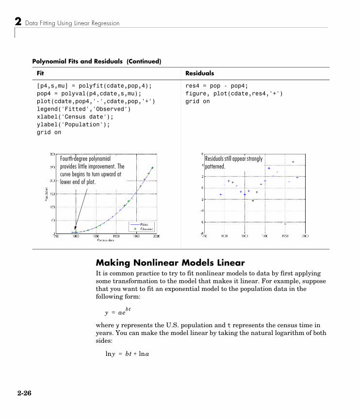
[p4,s,mu] = polyfit(cdate,pop,4);pop4 = polyval(p4,cdate,s,mu);plot(cdate,pop4,'-',cdate,pop,'+')legend('Fitted','Observed')xlabel('Census date');ylabel('Population');grid on
res4 = pop - pop4;figure, plot(cdate,res4,'+')grid on
Polynomial Fits and Residuals (Continued)
Fit Residuals
Fourth-degree polynomial provides little improvement. The curve begins to turn upward at lower end of plot.
Residuals still appear strongly patterned.
y aebt=
yln bt aln+=
6

Example — Fitting Data at the Command Line
If you plot ln(y) on the vertical axis and t on the horizontal axis, then ln(a) is the y-intercept and b is the slope of the straight line.
To fit a linear model to the transformed data, type at the command line
[logp1,s,mu] = polyfit(cdate,log(pop),1);logpred1 = exp(polyval(logp1,cdate,s,mu));semilogy(cdate,logpred1,'-',cdate,pop,'+');legend('Fitted','Observed')xlabel('Census date');ylabel('Log of Population');grid on
Confidence BoundsConfidence bounds are useful for determining how accurately you can estimate the value of the polynomial.
This example applies polyfit and polyval to the census sample data to produce confidence bounds for a second-order polynomial model.
Year values are normalized by polyfit, as described in “Center and Scale X Data” on page 2-6.
2-27

2 Data Fitting Using Linear Regression
2-2
The following syntax uses an interval of ±2∆, which corresponds to a 95% confidence interval:
[p2,s2,mu] = polyfit(cdate,pop,2);[pop2,del2] = polyval(p2,cdate,s2,mu);plot(cdate,pop,'+',cdate,pop2,'g-',cdate,pop2+2*del2,'r:',... cdate,pop2-2∗del2,'r:'); xlabel('Census date');ylabel('Population'), grid on
8

3
Analyzing Time Series from the Command LineAn introduction to the object-oriented command-line API for analyzing time-series data.
Introduction (p. 3-2) Brief description of the time-series objects
Creating timeseries Objects (p. 3-3) Instantiating the timeseries object
timeseries Functions (p. 3-11) Summary of timeseries functions
Creating Time-Series Collection Objects (p. 3-17)
Instantiating the tscollection object
tscollection Functions (p. 3-20) Summary of tscollection functions
Example — Analyzing Time-Series Data at the Command Line (p. 3-22)
How to analyze time-series data from the command line

3 Analyzing Time Series from the Command Line
3-2
IntroductionYou can analyze time-series data at the command line by using the following two MATLAB classes:
• timeseries — Contains data and time values, as well as the metadata information that includes units, events, data quality, and interpolation method
• tscollection — Contains a group of time-series objects that share a common time vector to enable operations on related groups of synchronized time series
The following auxiliary objects are available to define and store metadata for a time-series object:
• tsdata.event — Defines events
• tsdata.interpolation — Defines the interpolation method
For a detailed example that illustrates how to work with these objects at the command line, see “Example — Analyzing Time-Series Data at the Command Line” on page 3-22.
The API for working with time series is object-oriented, where
• Classes define properties and methods.
• Objects are intantiations of classes.
• You use a constructor to create an instance of an object, and use the set methods or dot notation to modify the properties of your objects.
For a detailed description of the rules of object-oriented programming in MATLAB, see MATLAB Classes and Objects in the MATLAB Programming documentation.
To learn how to work with the Time Series Tools graphical user interface (GUI) instead, see Chapter 4, “Using the Time Series Tools GUI.”

Creating timeseries Objects
Creating timeseries ObjectsThe time-series object, called timeseries, is a MATLAB variable that contains time-indexed data and data properties in a single, coherent structure. For example, in addition to data and time values, you can also use the time-series object to store events, descriptive information about data and time, data quality, and the interpolation method.
This section contains the following topics:
• “Observation vs. Data Sample” on page 3-3
• “Double vs. Date-String Time Vectors” on page 3-4
• “timeseries Constructor Syntax” on page 3-4
• “Properties of a timeseries Object” on page 3-5
Observation vs. Data SampleTo properly understand the description of the time-series API, it is important to clarify the difference between an observation and a data sample.
An observation is a single, scalar value recorded at a specific time.
A time-series data sample consists of one or more observations recorded at a specific time. The number of data samples in a time series is the same as the length of the time vector. If you create a time series that contains two data sets, each sample contains two values. The following table explains the size of a time-series data sample:
Data Sample Size
Type of Data Data-Sample Description
Vector with length N Scalar value
An N-by-M matrix with N samples
Vector with M values
An N-by-M-by-P-by-... multidimensional array with N samples
Multidimensional array of size M-by-P-by-...
3-3

3 Analyzing Time Series from the Command Line
3-4
Suppose that you have two redundant sensors simultaneously recording the same signal. The data collected by each of the sensors constitutes a complete set of observations. You can create a multivariate time-series object that contains several data sets (see “timeseries Constructor Syntax” on page 3-4). This is convenient when all data sets have the same units.
Alternatively, you can create one time-series object for each data set and then group them into a time-series collection. This is useful when the data sets have different units. For more information, see “tscollection Constructor Syntax” on page 3-17.
Double vs. Date-String Time VectorsThe time-series object enables you to specify time values as either double or date-string values.
timeseries Constructor SyntaxWorking with time-series data at the command line requires that you first create a time-series object.
The table below summarizes the syntax for creating a time-series object by using the timeseries constructor. For an example of using the constructor, see “Creating timeseries Objects” on page 3-23.
timeseries Constructor Syntax
Syntax Description
ts = timeseries Creates an empty timeseries object.
ts = timeseries(Data) Creates a time series with the specified Data.
Uses a default time vector that ranges from 0 to N-1 with a 1-second interval, where N is the number of samples.
ts = timeseries('Name') Creates an empty time series with the name specified by a string 'Name'. This name can be different from the time-series variable name.

Creating timeseries Objects
Properties of a timeseries ObjectThis table lists the properties of the timeseries object. You can specify Data, Time, Quality, Name, and IsTimeFirst properties as input arguments in the constructor. To assign other properties, use the set function or dot notation.
Note To get property information from the command line, type help timeseries/tsprops at the command line.
ts = timeseries(Data, Time) Creates a time series with the specified data array and time vector.
When time values are date strings, you must specify Time as a cell array of date strings.
ts = timeseries(Data, Time, Quality)
The Quality attribute is a vector of integers (-128 to 127) that specifies the quality in terms of codes defined by QualityInfo.Codes.
ts = timeseries(Data,..., 'Parameter', Value,...)
Optionally enter the following parameter-value pairs after the Data, Time, and Quality arguments:
• Name
• IsTimeFirst
• IsDatenum
Both Name and IsTimeFirst are described in “Properties of a timeseries Object” on page 3-5.
IsDatenum, when set to true, specifies that Time values are serial dates.
timeseries Constructor Syntax (Continued)
Syntax Description
3-5

3 Analyzing Time Series from the Command Line
3-6
For an example of editing time-series properties, see “Modifying Time-Series Units and Interpolation Method” on page 3-25.
timeseries Object Properties
Property Description
Data Time-series data, where each data sample corresponds to a set of observations in time.
The data can be a scalar, a vector, or a multidimensional array. Either the first or last dimension of the data must be aligned with Time.
By default, NaNs are used to represent missing or unspecified data. Set the TreatNaNasMissing property to determine how missing data is treated in calculations.
DataInfo Contains fields for storing contextual information about the Data:
• Unit — String that specifies data units
• Interpolation — A tsdata.interpolation object that specifies the interpolation method for this time series.
Fields of the tsdata.interpolation object:
- Fhandle — Function handle to the user-defined interpolation function
- Name — String that specifies the name of the interpolation method. Default methods include 'linear' and 'zoh' (zero-order hold). 'linear' is the default.
• UserData — Any user-defined information entered as a string
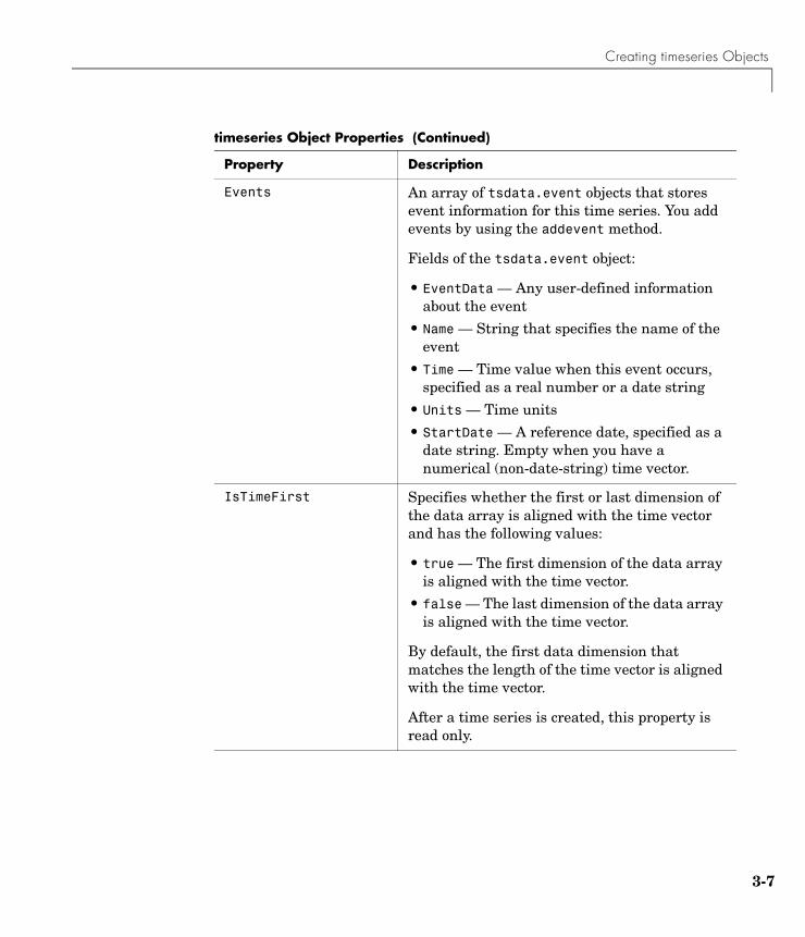
Creating timeseries Objects
Events An array of tsdata.event objects that stores event information for this time series. You add events by using the addevent method.
Fields of the tsdata.event object:
• EventData — Any user-defined information about the event
• Name — String that specifies the name of the event
• Time — Time value when this event occurs, specified as a real number or a date string
• Units — Time units
• StartDate — A reference date, specified as a date string. Empty when you have a numerical (non-date-string) time vector.
IsTimeFirst Specifies whether the first or last dimension of the data array is aligned with the time vector and has the following values:
• true — The first dimension of the data array is aligned with the time vector.
• false — The last dimension of the data array is aligned with the time vector.
By default, the first data dimension that matches the length of the time vector is aligned with the time vector.
After a time series is created, this property is read only.
timeseries Object Properties (Continued)
Property Description
3-7

3 Analyzing Time Series from the Command Line
3-8
Name Time-series name entered as a string. This name can be different from the name of the time-series variable in the MATLAB workspace.
Quality A vector or array of integers (-128 to 127) that specifies the quality in terms of codes defined by QualityInfo.Codes.
When Quality is a vector, it must have the same length as the time vector. In this case, each Quality value applies to a corresponding data sample.
When Quality is an array, it must have the same size as the data array. In this case, each Quality value applies to the corresponding element of the data array.
QualityInfo Provides a lookup table that converts numerical Quality codes to readable descriptions. QualityInfo fields include
• Codes — Vector of integers defining the “dictionary” of Quality codes that are assigned to each observation by the Quality vector or array
• Description — Cell array of strings, where each element provides a readable description of the associated quality code
• UserData — Stores any additional user-defined information
Length of Codes and Description must be the same.
timeseries Object Properties (Continued)
Property Description
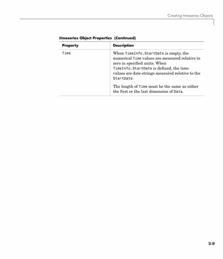
Creating timeseries Objects
Time When TimeInfo.StartDate is empty, the numerical Time values are measured relative to zero in specified units. When TimeInfo.StartDate is defined, the time values are date strings measured relative to the StartDate.
The length of Time must be the same as either the first or the last dimension of Data.
timeseries Object Properties (Continued)
Property Description
3-9
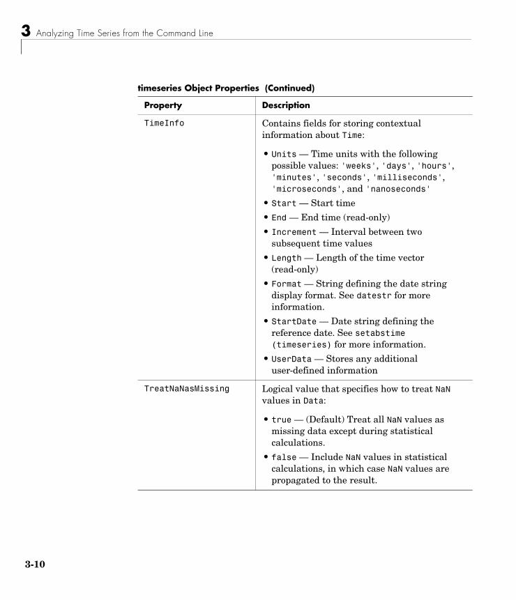
3 Analyzing Time Series from the Command Line
3-1
TimeInfo Contains fields for storing contextual information about Time:
• Units — Time units with the following possible values: 'weeks', 'days', 'hours', 'minutes', 'seconds', 'milliseconds', 'microseconds', and 'nanoseconds'
• Start — Start time
• End — End time (read-only)
• Increment — Interval between two subsequent time values
• Length — Length of the time vector (read-only)
• Format — String defining the date string display format. See datestr for more information.
• StartDate — Date string defining the reference date. See setabstime (timeseries) for more information.
• UserData — Stores any additional user-defined information
TreatNaNasMissing Logical value that specifies how to treat NaN values in Data:
• true — (Default) Treat all NaN values as missing data except during statistical calculations.
• false — Include NaN values in statistical calculations, in which case NaN values are propagated to the result.
timeseries Object Properties (Continued)
Property Description
0

timeseries Functions
timeseries FunctionsThe following categories of functions are available for working with timeseries objects:
• “General timeseries Functions” on page 3-12
• “Data and Time Manipulation” on page 3-12
• “Events” on page 3-14
• “Arithmetic Operations” on page 3-15
• “Statistical Functions” on page 3-15
3-11

3 Analyzing Time Series from the Command Line
3-1
General timeseries Functions
Data and Time Manipulation
General timeseries Functions
Function Description
get (timeseries) Query timeseries property values
getqualitydesc Return data quality descriptions based on the Quality values assigned to a timeseries object
getdatasamplesize Return the size of each data sample for a timeseries object
isempty (timeseries)
Evaluate to true for an empty timeseries object
length (timeseries)
Return the length of the time vector
plot (timeseries) Plot the time series
size (timeseries) Return the size property of a time series
set (timeseries) Set specific timeseries property values
Manipulate Time-Series Data and Time
Function Description
addsample Add one sample to a timeseries object
ctranspose (timeseries)
Transpose a timeseries object
delsample Delete a sample from a timeseries object
detrend (timeseries) Subtract the mean or best-fit line and remove all NaNs from a time series
filter (timeseries) Shape the time-series data by using a 1-D digital filter
2
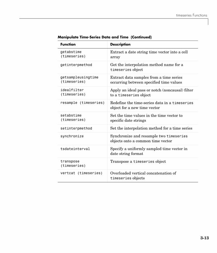
timeseries Functions
getabstime (timeseries)
Extract a date string time vector into a cell array
getinterpmethod Get the interpolation method name for a timeseries object
getsampleusingtime (timeseries)
Extract data samples from a time series occurring between specified time values
idealfilter (timeseries)
Apply an ideal pass or notch (noncausal) filter to a timeseries object
resample (timeseries) Redefine the time-series data in a timeseries object for a new time vector
setabstime (timeseries)
Set the time values in the time vector to specific date strings
setinterpmethod Set the interpolation method for a time series
synchronize Synchronize and resample two timeseries objects onto a common time vector
tsdateinterval Specify a uniformly sampled time vector in date string format
transpose (timeseries)
Transpose a timeseries object
vertcat (timeseries) Overloaded vertical concatenation of timeseries objects
Manipulate Time-Series Data and Time (Continued)
Function Description
3-13
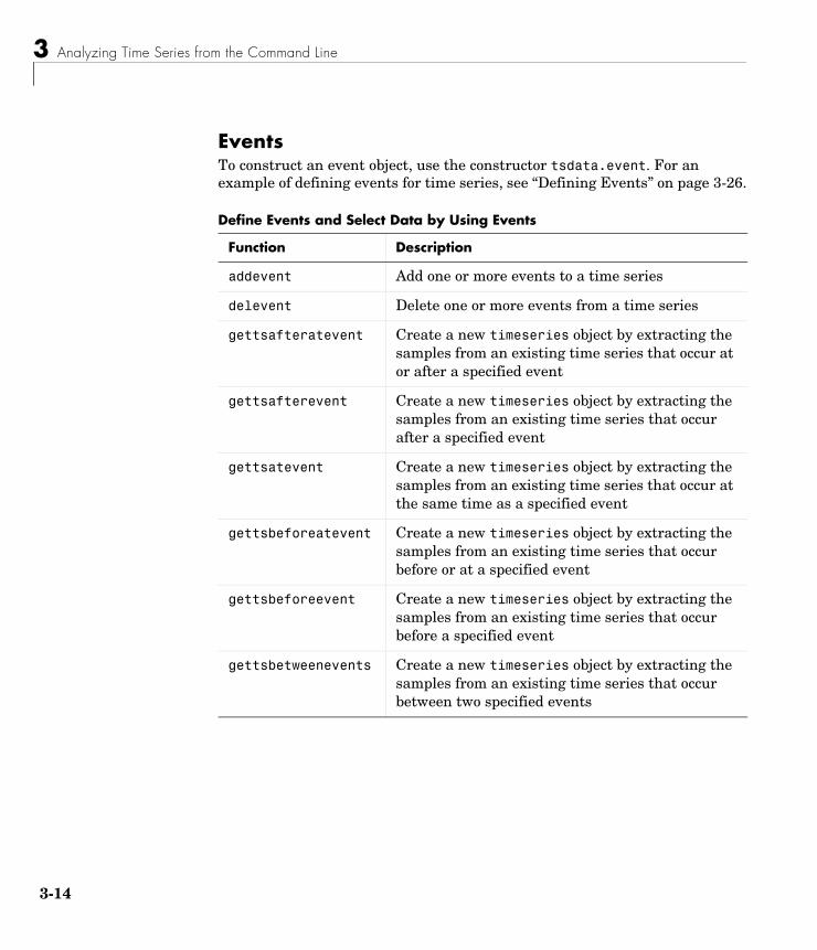
3 Analyzing Time Series from the Command Line
3-1
EventsTo construct an event object, use the constructor tsdata.event. For an example of defining events for time series, see “Defining Events” on page 3-26.
Define Events and Select Data by Using Events
Function Description
addevent Add one or more events to a time series
delevent Delete one or more events from a time series
gettsafteratevent Create a new timeseries object by extracting the samples from an existing time series that occur at or after a specified event
gettsafterevent Create a new timeseries object by extracting the samples from an existing time series that occur after a specified event
gettsatevent Create a new timeseries object by extracting the samples from an existing time series that occur at the same time as a specified event
gettsbeforeatevent Create a new timeseries object by extracting the samples from an existing time series that occur before or at a specified event
gettsbeforeevent Create a new timeseries object by extracting the samples from an existing time series that occur before a specified event
gettsbetweenevents Create a new timeseries object by extracting the samples from an existing time series that occur between two specified events
4

timeseries Functions
Arithmetic Operations
Statistical Functions
Overloaded Arithmetic Operations
Operation Description
+ Add the corresponding elements of time series
- Subtract the corresponding elements of time series
.* Element-by-element multiplication of time series
* Matrix-multiply two time series
./ Right element-by-element division of time series
/ Right matrix division of time series
.\ Element-by-element left-array divide
\ Left matrix division of time series
Overloaded Statistical Functions
Function Description
iqr (timeseries)
Return the interquartile range of the time-series data
max (timeseries)
Return the maximum value of the time-series data
mean (timeseries)
Return the mean of the time-series data
median (timeseries)
Return the median of the time-series data
min (timeseries)
Return the minimum of the time-series data
std (timeseries)
Return the standard deviation of the time-series data
3-15

3 Analyzing Time Series from the Command Line
3-1
sum (timeseries)
Return the sum of the time-series data
var (timeseries)
Return the variance of the time-series data
Overloaded Statistical Functions
Function Description
6

Creating Time-Series Collection Objects
Creating Time-Series Collection ObjectsA time-series collection object, called tscollection, is a MATLAB variable that groups several time series with a common time vector. The time series that you include in the tscollection are called members of this collection.
MATLAB provides several functions for convenient analysis and manipulation of time series in a tscollection object.
tscollection Constructor SyntaxWorking with a time-series collection at the command line requires that you first create a tscollection object.
The table below summarizes the syntax for creating a time-series collection object by using the tscollection constructor. For an example of creating a tscollection object, see “Creating a Time-Series Collection” on page 3-26.
tscollection Contructor Syntax
Syntax Description
tsc = tscollection(TimeSeries)
Creates a tscollection object with one or more timeseries objects already created in the MATLAB workspace.
The argument TimeSeries can be a
• Single timeseries object
• Cell array of timeseries objects
The TimeSeries objects share a common vector in the time-series collection.
3-17

3 Analyzing Time Series from the Command Line
3-1
tsc = timeseries(Time) Creates an empty tscollection object with the time vector Time.
When time values are date strings, you must specify Time as a cell array of date strings.
ts = timeseries(Time, TimeSeries, 'Parameter', Value,...)
Optionally enter the following parameter-value pairs after the Time and TimeSeries arguments:
• Name• IsDatenum
Name is described in “Properties of tscollection Objects” on page 3-19.
When set to true, IsDatenum specifies that the Time values are serial dates.
tscollection Contructor Syntax
Syntax Description
8
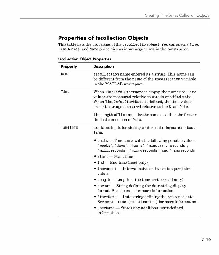
Creating Time-Series Collection Objects
Properties of tscollection ObjectsThis table lists the properties of the tscollection object. You can specify Time, TimeSeries, and Name properties as input arguments in the constructor.
tscollection Object Properties
Property Description
Name tscollection name entered as a string. This name can be different from the name of the tscollection variable in the MATLAB workspace.
Time When TimeInfo.StartDate is empty, the numerical Time values are measured relative to zero in specified units. When TimeInfo.StartDate is defined, the time values are date strings measured relative to the StartDate.
The length of Time must be the same as either the first or the last dimension of Data.
TimeInfo Contains fields for storing contextual information about Time:
• Units — Time units with the following possible values: 'weeks', 'days', 'hours', 'minutes', 'seconds', 'milliseconds', 'microseconds', and 'nanoseconds'
• Start — Start time
• End — End time (read-only)
• Increment — Interval between two subsequent time values
• Length — Length of the time vector (read-only)
• Format — String defining the date string display format. See datestr for more information.
• StartDate — Date string defining the reference date. See setabstime (tscollection) for more information.
• UserData — Stores any additional user-defined information
3-19

3 Analyzing Time Series from the Command Line
3-2
tscollection FunctionsThe following categories of functions are available for working with time-series collection objects:
• “General tscollection Functions” on page 3-20
• “Data and Time Manipulation” on page 3-20
General tscollection Functions
Data and Time Manipulation
General tscollection Functions
Function Description
get (tscollection)
Query tscollection property values
isempty (tscollection)
Evaluate to true for an empty tscollection object
length (tscollection)
Return the length of the time vector
plot (timeseries) Plot individual time series in a collection
size (tscollection)
Return the size of a tscollection object
set (tscollection)
Set tscollection property values
Manipulate tscollection Data and Time
Function Description
addts Add a timeseries object to a tscollection
addsampletocollection Add data samples to a tscollection
0

tscollection Functions
delsamplefromcollection Delete data samples from a tscollection object
getabstime (tscollection) Extract a date string time vector into a cell array
getsampleusingtime (tscollection)
Extract data samples from a tscollection occurring between specified time values
gettimeseriesnames Return a cell array of names of time series in a tscollection
horzcat (tscollection) Overloaded horizontal concatenation of tscollection objects. Combines several timeseries objects with the same time vector into one time-series collection.
removets Remove one or more timeseries objects from a tscollection
resample (tscollection) Redefine a tscollection object on a new time vector
setabstime (tscollection) Set the time values in the time vector of a tscollection to specific date strings
settimeseriesnames Change the name of the selected timeseries object in a tscollection
vertcat (tscollection) Overloaded vertical concatenation of tscollection objects. Joins time series collections along the time dimension.
Manipulate tscollection Data and Time (Continued)
Function Description
3-21

3 Analyzing Time Series from the Command Line
3-2
Example — Analyzing Time-Series Data at the Command Line
This example describes the sample data and illustrates several common tasks:
• “About the Example Data” on page 3-22
• “Creating timeseries Objects” on page 3-23
• “Modifying Time-Series Units and Interpolation Method” on page 3-25
• “Defining Events” on page 3-26
• “Creating a Time-Series Collection” on page 3-26
• “Resampling the tscollection” on page 3-27
• “Adding a Data Sample to the Tscollection” on page 3-27
• “Handling Missing Data” on page 3-28
• “Removing a Time Series from the Collection” on page 3-28
• “Changing a Numerical Time Vector to Date Strings” on page 3-28
• “Plotting tscollection Members” on page 3-29
About the Example DataThe following table contains a data set with hourly traffic counts at three road intersections in the same town, collected over a 24-hour period.
Hourly Traffic Counts
Time (Hour) Intersection 1 Intersection 2 Intersection 3
1 11 11 9
2 7 13 11
3 14 17 20
4 11 13 9
5 43 51 69
6 38 46 76
7 61 132 186
2

Example — Analyzing Time-Series Data at the Command Line
Creating timeseries ObjectsThis portion of the example illustrates how to create several timeseries objects from an array.
%% Import the sample dataload count.dat
This adds the variable count to the MATLAB workspace.
8 75 135 180
9 38 88 115
10 28 36 55
11 12 12 14
12 18 27 30
13 18 19 29
14 17 15 18
15 19 36 48
16 32 47 10
17 42 65 92
18 57 66 151
19 44 55 90
20 114 145 257
21 35 58 68
22 11 12 15
23 13 9 15
24 10 9 7
Hourly Traffic Counts (Continued)
Time (Hour) Intersection 1 Intersection 2 Intersection 3
3-23
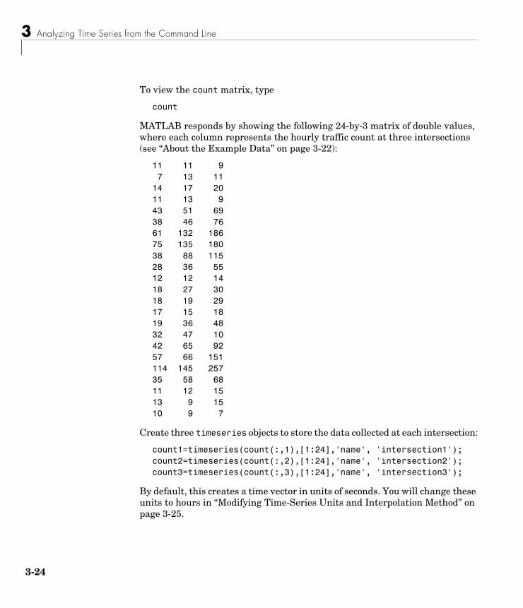
3 Analyzing Time Series from the Command Line
3-2
To view the count matrix, type
count
MATLAB responds by showing the following 24-by-3 matrix of double values, where each column represents the hourly traffic count at three intersections (see “About the Example Data” on page 3-22):
11 11 97 13 1114 17 2011 13 943 51 6938 46 7661 132 18675 135 18038 88 11528 36 5512 12 1418 27 3018 19 2917 15 1819 36 4832 47 1042 65 9257 66 151114 145 25735 58 6811 12 1513 9 1510 9 7
Create three timeseries objects to store the data collected at each intersection:
count1=timeseries(count(:,1),[1:24],'name', 'intersection1');count2=timeseries(count(:,2),[1:24],'name', 'intersection2');count3=timeseries(count(:,3),[1:24],'name', 'intersection3');
By default, this creates a time vector in units of seconds. You will change these units to hours in “Modifying Time-Series Units and Interpolation Method” on page 3-25.
4

Example — Analyzing Time-Series Data at the Command Line
Modifying Time-Series Units and Interpolation MethodAfter you have created the timeseries object, you can modify its properties by using dot notation.
To view the current time-series properties, issue the get (timeseries) command.
get(count1)
MATLAB responds by displaying the current property values of the count1 timeseries object:
Events: [] Name: 'intersection1'Data: [24x1 double]DataInfo: [1x1 tsdata.datametadata]Time: [24x1 double]TimeInfo: [1x1 tsdata.timemetadata]Quality: []QualityInfo: [1x1 tsdata.qualmetadata]IsTimeFirst: trueTreatNaNasMissing: true
To view the current DataInfo properties, use dot notation.
count1.DataInfo
Then change the data units and the default interpolation method for count1:
count1.DataInfo.Units = 'cars'; % Specify new data unitscount1.DataInfo.Interpolation = tsdata.interpolation('zoh');
% Set the interpolation method to zero-order hold
To verify that the DataInfo properties have been modified, type
count1.datainfo
MATLAB confirms the change by displaying
Time Series Data Meta Data Object Unit cars Interpolation Method zoh
3-25

3 Analyzing Time Series from the Command Line
3-2
Modify the time units to be 'hours' for the three time series:
count1.TimeInfo.Units = 'hours';count2.TimeInfo.Units = 'hours';count3.TimeInfo.Units = 'hours';
Defining EventsYou can add two events to the data to indicate the times of the AM commute and PM commute by using the following syntax:
%% Construct and add the first event to all time seriese1 = tsdata.event('AMCommute',8);
% Construct the first event at 8 AMe1.Units = 'hours'; % Specify the time units of the timecount1 = addevent(count1,e1); % Add the event to count1count2 = addevent(count2,e1); % Add the event to count2count3 = addevent(count3,e1); % Add the event to count3
%% Construct and add the second event to all time seriese2 = tsdata.event('PMCommute',18);
% Construct the first event at 6 PMe2.Units = 'hours'; % Specify the time units of the timecount1 = addevent(count1,e2); % Add the event to count1count2 = addevent(count2,e2); % Add the event to count2count3 = addevent(count3,e2); % Add the event to count3
Creating a Time-Series CollectionCreate a tscollection object named count_coll and add to it two out of three time series already in the MATLAB workspace, by using the following syntax:
tsc=tscollection({count1 count2},'name', 'count_coll')
MATLAB responds with
Time Series Collection Object: count_collTime vector characteristicsStart time 1 hoursEnd time 24 hoursMember Time Series Objects: intersection1 intersection2
6

Example — Analyzing Time-Series Data at the Command Line
Note that the Name property of the time series is used to name the collection members as intersection1 and intersection2.
Add the third time series in the workspace by using the following syntax:
tsc=addts(tsc, count3)
MATLAB now lists all three time series as members in the collection:
Time Series Collection Object: count_collTime vector characteristicsStart time 1 hoursEnd time 24 hoursMember Time Series Objects: intersection1 intersection2
intersection3
Resampling the tscollectionResampling a tscollection object casts its members onto a new time vector. Any new data points are calculated using the default interpolation method you associated with the time series.
To resample the time series for every half hour and save it as a new collection object, enter the following syntax:
tsc1=resample(tsc,[1:0.5:24])
The new tscollection variable is tsc1. The new data points in the intersection1 member are calculated by using the zero-order hold interpolation method, as specified in “Modifying Time-Series Units and Interpolation Method” on page 3-25. The new data points in intersection2 and intersection3 are calculated using linear interpolation (by default).
Adding a Data Sample to the TscollectionYou can add a new data sample to the tscollection at 3.3 hours.
The following syntax only specifies data for the intersection1 member:
tsc1=addsampletocollection(tsc1,'time',3.3,'intersection1',5)
3-27

3 Analyzing Time Series from the Command Line
3-2
There are currently three members in the tsc1 collection. Because you did not specify the data values for the intersection2 and intersection3 time-series members in the new sample, the missing values are represented by NaNs.
Handling Missing DataMissing time-series data is represented by NaNs in the time series. When you perform data analysis, you might want to either remove the missing data or interpolate it by using the interpolation method you specified for that time series.
Removing Missing DataTo remove all data samples containing NaN values, enter the following syntax:
tsc1=delsamplefromcollection(tsc1,'index',...find(isnan(tsc1.intersection2.data)));
Interpolating Missing DataBecause the sample with missing data was removed by the previous command, add the data sample again to reintroduce NaN values in intersection2 and intersection3 as follows:
tsc1=addsampletocollection(tsc1,'time',3.3,'intersection1',5);
To interpolate the missing values in the time-series collection, use the resample function:
tsc1=resample(tsc1,tsc1.Time)
Removing a Time Series from the CollectionTo remove the 'intersection3' time series from the tscollection, issue the following command:
tsc1=removets(tsc1,'intersection3')
Changing a Numerical Time Vector to Date StringsTo convert a numerical time vector to date strings, you must set the StartDate field of the TimeInfo property. For example, suppose the reference date occurs on December 25, 2004:
tsc.TimeInfo.StartDate='DEC-25-2004 00:00:00';
8

Example — Analyzing Time-Series Data at the Command Line
To verify that the time vector now uses date strings, type the following command to look at the sixth element of the intersection2 member (which was previously interpolated):
tsc1.intersection2(6)
MATLAB returns
Time Series Object: unnamedTime vector characteristics Length 1 Start date 25-Dec-2004 03:18:00 End date 25-Dec-2004 03:18:00Data characteristics Interpolation method linear Size [1 1] Data type doubleTime Data Quality-------------------------------------------------------------25-Dec-2004 03:18:00 15.8
Note that the sixth element of the intersection2 member has an interpolated data value of 15.8 cars at 3.3 hours (or 3:18:00). This data value was previously a NaN when you added a new data sample to the time-series collection without specifying the data for this time-series member (see “Adding a Data Sample to the Tscollection” on page 3-27).
Plotting tscollection MembersYou can plot the two remaining time-series members in the tsc1 time-series collection by using the following sequence of commands:
plot(tsc1.intersection1); hold on;plot(tsc1.intersection2)
3-29

3 Analyzing Time Series from the Command Line
3-3
This plot shows the two time series in the collection: intersection1 and intesection2. intersection1 uses the zero-order hold interpolation method and therefore has a jagged curve. In contrast, intersection2 uses a linear interpolation method.
The circles on the plot indicate events, as defined in “Defining Events” on page 3-26.
0

4
Using the Time Series Tools GUIDescribes how to use the MATLAB Time Series Tools graphical user interface (GUI) for analyzing time-series data.
Introduction (p. 4-2) A brief overview of the Time Series Tools GUI and the typical workflow
Importing Data into Time Series Tools (p. 4-9)
Summary of supported data sources; instructions for importing the data into Time Series Tools from MATLAB, Simulink, and other data sources; handling missing data
Editing Data, Time, Attributes, and Events (p. 4-15)
How to access the GUI for editing time-series data, time, units, interpolation method, quality codes, and events
Working with Time Plots (p. 4-17) Creating a time plot and modifying the plot properties
Selecting Time-Series Data (p. 4-25) How to select the time-series data in a time plot on which you want to focus the analysis
Working with a Histogram (p. 4-29) Creating a histogram and modifying plot properties
Working with a Spectral Plot (p. 4-33) Creating a spectral plot and modifying plot properties
Working with a Correlogram (p. 4-39) Creating an autocorrelation plot and modifying plot properties
Comparing Time Series (p. 4-43) Creating an XY and a cross-correlation plot to compare time series
Example — Analyzing Time-Series Data with Time Series Tools (p. 4-47)
An example to illustrate importing, plotting, and analyzing time-series data

4 Using the Time Series Tools GUI
4-2
IntroductionThe Time Series Tools graphical user interface (GUI) extends the MATLAB environment for analyzing both time- and frequency-domain time-series data.
For more information about working with time-series data from the command line, see Chapter 3, “Analyzing Time Series from the Command Line.”
This section contains the following topics:
• “Starting Time Series Tools” on page 4-2
• “Time Series Tools Window” on page 4-3
• “Workflow in Time Series Tools” on page 4-4
• “Time-Series Analysis Operations” on page 4-5
• “Plots in Time Series Tools” on page 4-6
• “Customizing Plot Line and Marker Styles” on page 4-7
• “Automatic M-Code Generation” on page 4-7
• “Getting Help” on page 4-7
Starting Time Series ToolsTo start Time Series Tools, type
tstool
in the MATLAB Command Window.
This opens the Time Series Tools GUI without loading any data. To learn how to import data into Time Series Tools, see “Importing Data into Time Series Tools” on page 4-9.
Alternatively, you can start Time Series Tools and simultaneously import the data from the MATLAB workspace, including
• Time-series objects (see “Creating timeseries Objects” on page 3-3)
• Time-series collection objects (see “Creating Time-Series Collection Objects” on page 3-17)
• Simulink® logged signals (see the Simulink documentation about enabling signal logging in Simulink models)

Introduction
Note If a Simulink logged signal Name property contains a “/”, the entire logged signal — including all levels of the signal hierarchy — is not imported into Time Series Tools.
The following table summarizes the command-line syntax for starting Time Series Tools and loading data from the MATLAB workspace:
Time Series Tools WindowThe Time Series Tools window consists of the following three areas:
• Time Series Session tree — Organizes time-series data, Simulink time-series data, and the Views (or plots) you create from this data. The Simulink Time Series node is shown only when you have Simulink installed on your computer.
Tip The quickest way to create plots is by dragging and dropping time series or collections into a Views node that corresponds to the kind of plot you want.
• Application pane — Located to the right of the tree, it enables operations on the selected data or plot node in the tree.
Syntax for Loading Data from the MATLAB Workspace
To Load... Syntax Description
Time series tstool(tsname) tsname is the name of a time-series object.
Time-series collections
tstool(tscname) tscname is the name of a time-series collection object.
Simulink logged signals
tstool(sldata) sldata is the name of the variable that represents logged-signal data from a Simulink model.
4-3

4 Using the Time Series Tools GUI
4-4
• Context-sensitive help pane — Located on the far right of the Time Series Tools window, it provides brief instructions for working with the application pane GUI. For more information, see “Getting Help” on page 4-7.
Workflow in Time Series ToolsA typical workflow with Time Series Tools might include the following tasks:
1 Importing data from an Excel Workbook, MAT-file, MATLAB workspace, or Simulink logged-signal data (see “Importing Data into Time Series Tools” on page 4-9)
2 Creating a time plot (see “Working with Time Plots” on page 4-17) or histogram (see “Working with a Histogram” on page 4-29) to explore the data
3 Selecting a subset of the data for analysis (see “Selecting Time-Series Data” on page 4-25)
����������������� ������������������ ������������� ���������������������
�� ����������������������������������������������������������������� ���
���������������������������� ���������������������
������������������������������������������������������� ���

Introduction
4 Preparing the data for analysis by
- Correcting errors (see “Editing Data, Time, Attributes, and Events” on page 4-15)
- Modifying outliers (see “Selecting Data by Using Rules” on page 4-26)
- Interpolating or removing missing observations (see “Handling Missing Data” on page 4-12)
5 Generating derived plots to gain further insight into your data, such as
- Spectral plots (see “Working with a Spectral Plot” on page 4-33)
- Autocorrelation plots (see “Working with a Correlogram” on page 4-39)
- XY plots (see “Creating an XY Plot” on page 4-43)
- Cross-correlation plots (see “Creating a Cross-Correlation Plot” on page 4-44)
6 Exporting data from Time Series Tools to the MATLAB workspace, Excel worksheet, or MAT-file.
Time-Series Analysis OperationsThe following table summarizes the operations you can perform on an individual time series or on a time-series collection. These operations are available from the Data menu in Time Series Tools after you select the time series or collection node in the tree.
You can access on-the-spot instructions via the Help button in the Time Series Tools dialogs.
Summary of Time-Series Data Analysis Operations
Data Menu Item Description
Remove Missing Data
Delete the times that contain missing data
Detrend Subtract a constant or a linear trend from the data
Filter Smooth and shape the time-series data
4-5
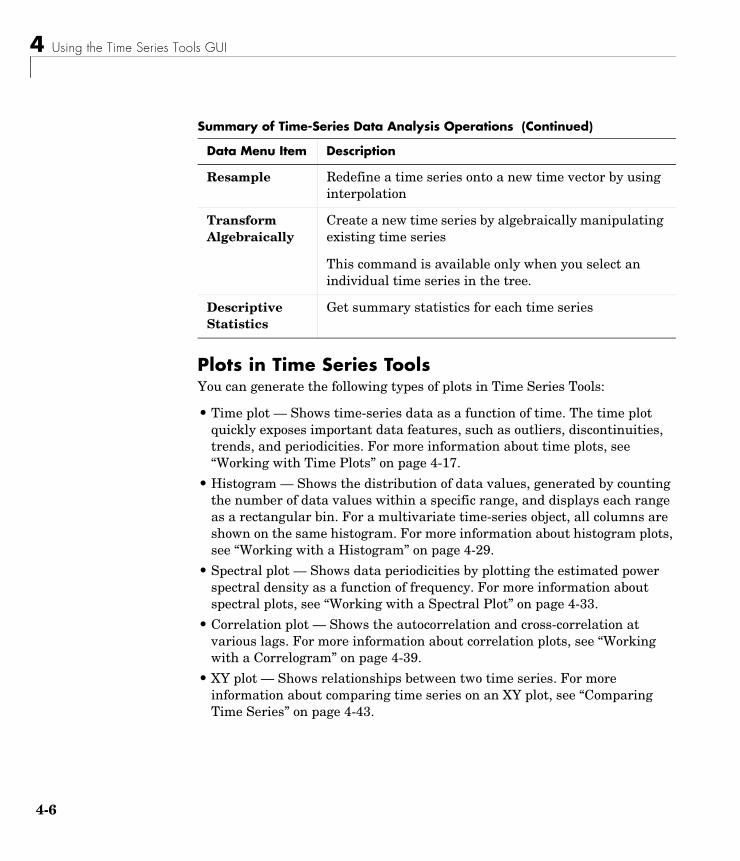
4 Using the Time Series Tools GUI
4-6
Plots in Time Series ToolsYou can generate the following types of plots in Time Series Tools:
• Time plot — Shows time-series data as a function of time. The time plot quickly exposes important data features, such as outliers, discontinuities, trends, and periodicities. For more information about time plots, see “Working with Time Plots” on page 4-17.
• Histogram — Shows the distribution of data values, generated by counting the number of data values within a specific range, and displays each range as a rectangular bin. For a multivariate time-series object, all columns are shown on the same histogram. For more information about histogram plots, see “Working with a Histogram” on page 4-29.
• Spectral plot — Shows data periodicities by plotting the estimated power spectral density as a function of frequency. For more information about spectral plots, see “Working with a Spectral Plot” on page 4-33.
• Correlation plot — Shows the autocorrelation and cross-correlation at various lags. For more information about correlation plots, see “Working with a Correlogram” on page 4-39.
• XY plot — Shows relationships between two time series. For more information about comparing time series on an XY plot, see “Comparing Time Series” on page 4-43.
Resample Redefine a time series onto a new time vector by using interpolation
Transform Algebraically
Create a new time series by algebraically manipulating existing time series
This command is available only when you select an individual time series in the tree.
Descriptive Statistics
Get summary statistics for each time series
Summary of Time-Series Data Analysis Operations (Continued)
Data Menu Item Description
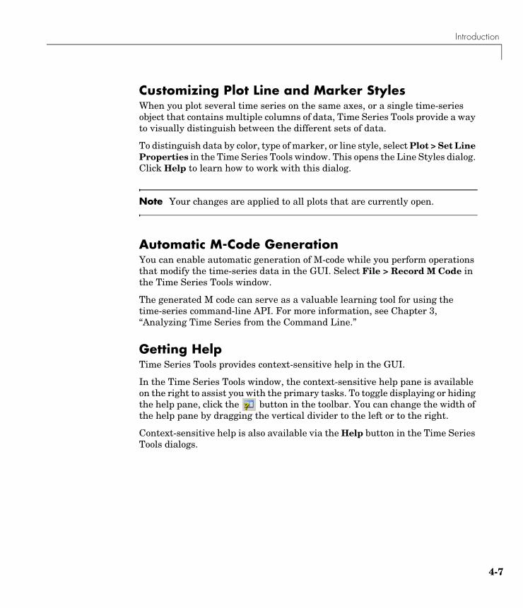
Introduction
Customizing Plot Line and Marker StylesWhen you plot several time series on the same axes, or a single time-series object that contains multiple columns of data, Time Series Tools provide a way to visually distinguish between the different sets of data.
To distinguish data by color, type of marker, or line style, select Plot > Set Line Properties in the Time Series Tools window. This opens the Line Styles dialog. Click Help to learn how to work with this dialog.
Note Your changes are applied to all plots that are currently open.
Automatic M-Code GenerationYou can enable automatic generation of M-code while you perform operations that modify the time-series data in the GUI. Select File > Record M Code in the Time Series Tools window.
The generated M code can serve as a valuable learning tool for using the time-series command-line API. For more information, see Chapter 3, “Analyzing Time Series from the Command Line.”
Getting HelpTime Series Tools provides context-sensitive help in the GUI.
In the Time Series Tools window, the context-sensitive help pane is available on the right to assist you with the primary tasks. To toggle displaying or hiding the help pane, click the button in the toolbar. You can change the width of the help pane by dragging the vertical divider to the left or to the right.
Context-sensitive help is also available via the Help button in the Time Series Tools dialogs.
4-7

4 Using the Time Series Tools GUI
4-8
In the Time Series Tools Import Wizard, you can also access field-level help to assist you with importing data, as follows:
1 Right-click the text label of a field on which you want to get help.
2 Select What's This from the shortcut menu.

Importing Data into Time Series Tools
Importing Data into Time Series ToolsAfter starting Time Series Tools, you can import the data from a file or from the MATLAB workspace.
This section contains the following topics:
• “Types of Data Sources” on page 4-9
• “Observation vs. Data Sample” on page 4-10
• “How to Import Data” on page 4-10
• “Changes to the Data During Import” on page 4-11
• “Handling Missing Data” on page 4-12
• “Importing Multivariate Data” on page 4-12
Types of Data SourcesYou can import the following kinds of data into Time Series Tools from a file or from the MATLAB workspace:
• Raw data from an Excel file, MAT-file, or an array in the MATLAB workspace
The Import Wizard in Time Series Tools facilitates assigning a time vector to the data during import. You can either import the time vector or define a uniformly-spaced time vector.
Note You use the Import Wizard in Time Series Tools specifically to create time-series objects. This is different from the Import Wizard you access from the MATLAB Command Window, which imports data as MATLAB vectors and matrices.
• Timeseries or tscollection objects in the MATLAB workspace
For more information about creating these objects, see Chapter 3, “Analyzing Time Series from the Command Line.”
• Simulink® logged-signal data from a Simulink model
For more information about enabling signal logging in Simulink models, see the Simulink documentation.
4-9

4 Using the Time Series Tools GUI
4-1
Observation vs. Data SampleTo properly understand importing time-series data, it is important to clarify the difference between an observation and a data sample.
An observation is a single scalar value recorded at a specific time.
A time-series data sample consists of one or more observations recorded at a specific time. The number of data samples in a time series is the same as the length of the time vector. If you create a time series that contains two data columns, the size of each sample contains two values. The following table explains the size of a time-series data sample:
Suppose that you have two redundant sensors simultaneously recording the same signal. The data collected by each of the sensors constitutes a complete set of observations. When importing the data, you can create a multivariate time-series object that contains several observation sets. This is convenient when all data sets have the same units.
Alternatively, you can create one time-series object for each data set and then group them into a time-series collection. This is useful when the data sets have different units. For more information, see “From Raw Data to a Time-Series Collection” on page 4-13.
How to Import DataThe following table summarizes how to access the GUI for importing data into Time Series Tools from each of the supported data sources. After you open the appropriate GUI, you can get additional instructions by clicking Help.
Data Sample Size
Type of Data Data-Sample Description
A vector with length N Scalar value
An N x M matrix with N samples
Vector with M values
0

Importing Data into Time Series Tools
Each time series you import or create by using the Import Wizard is added as a node to the Time Series Session tree in the Time Series Tools window.
Note You cannot import a timeseries or tscollection object from a MAT-file.
Changes to the Data During ImportWhen you import data into Time Series Tools, a copy of the data is imported without affecting the original data source. The copy in Time Series Tools is automatically modified as follows:
• Rowwise data is transposed to become columnwise with the time vector in the first column.
• Non-double data, such as int, logical, and fixed-point, is converted to double.
• Missing data values are replaced by NaNs.
• Sparse matrix is converted to full matrix.
• Data that has more than two dimensions is reshaped to two dimensions such that dimensions three and higher become additional columns in the data table. For example, a 2-by-3-by-5 data array becomes a 2-by-15 data array (when time is aligned with the first dimension).
Type of Data Source File Menu Command
Excel Worksheet (.xls file) data table
Create Time Series from File
MAT-file array Create Time Series from File
MATLAB workspace array Import from Workspace > Array Data
Time-series or collection object in the MATLAB workspace
Import from Workspace > Time Series or Collection Object
Simulink logged-signal data Import from Workspace > Simulink Data Logs
4-11

4 Using the Time Series Tools GUI
4-1
Caution When exporting the data you imported into Time Series Tools, note that it might differ from the original data you imported.
Handling Missing DataWhen you import data from an Excel Worksheet that contains missing values into Time Series Tools, the missing data is automatically replaced with NaNs.
You can also deliberately replace selected data with NaNs, as described in “Selecting Time-Series Data” on page 4-25.
Time Series Tools enables you to handle missing data in the Process Data dialog by performing the following operations:
• Interpolate missing values using the method specified in “Editing Data, Time, Attributes, and Events” on page 4-15.
You can interpolate either by using the existing data in the current time series, or the interpolated data value at the same time from another time series.
• Remove samples with missing values.
To open the Process Data dialog from the Time Series Tools window,
1 Select a time series or a collection in the Time Series Session tree.
2 Select Data > Interpolate or Data > Remove Missing Data.
3 In the Process Data dialog, click Help to access context-sensitive help.
Importing Multivariate DataWhen data consists of several related variables, you might want to keep these observations synchronized during data analysis.
There are two ways to prepare multivariate data in Time Series Tools for synchronized analysis:
• Create a time-series collection with a common time vector, where each variable is a member of the collection.
2

Importing Data into Time Series Tools
• Import several data sets into a single time-series object such that each variable becomes a column in the time-series object.
Choosing How to Represent Multivariate DataWhether you choose to represent multivariate data as several time series in a collection or a single time series with several columns depends on how you want to label your data. In either case, the data remains synchronized after manipulation and transformation.
When your data set contains different quantities that must be distinguished during analysis, then it is better to store each quantity as a separate time series and then group them into a collection. For example, if you are working with the stock-price data in a portfolio, you might want to represent each stock as a separate time series.
Suppose you have a data set consisting of several redundant sensor measurements: all sensors are recording the same quantity. In this case, it might be best to store the entire data set in a single time-series object.
From Raw Data to a Time-Series CollectionThe following procedure outlines a simple way to create a time-series collection from a multivariate data set, which comes from either an Excel workbook or a MATLAB array.
At each step, you can click the Help button in the GUI to access context-sensitive help.
1 To import each data set as a separate time series, select File > Import > Raw Data in Time Series Tools to open the Import Wizard.
2 After importing the data, select the Time Series node in the tree and export all time series from Time Series Tools to the MATLAB workspace.
3 In the MATLAB Command Window, combine the individual time series into a time-series collection object. For an example of creating a time-series collection from individual time series, see “Creating a Time-Series Collection” on page 3-26.
4 In Time Series Tools, select File > Import > Time Series or Collection Object to import the time-series collection from the MATLAB workspace.
4-13

4 Using the Time Series Tools GUI
4-1
5 Perform analysis tasks on the time-series collection. For a list of the kinds of tasks you can perform, see “Workflow in Time Series Tools” on page 4-4.
4

Editing Data, Time, Attributes, and Events
Editing Data, Time, Attributes, and EventsTime Series Tools provides an easy way to edit time-series data, time, attributes, and events.
Time-series attributes consist of the following:
• Data quality codes — Used to annotate the quality of each value in the data table
• Data units — Used to annotate the data axis on plots
• Interpolation method — Used by default for this time series to fill in missing data or to resample the data onto a new time vector
You use events to mark the data at a specific time in the data table and on a plot. Events also provide a convenient way to synchronize the data for multiple time series.
To display the interface for editing time series and adding events, select the time-series data node in the tree and follow the instructions in the context-sensitive help pane.
Note To toggle displaying and hiding the help pane, click the button in the toolbar.
4-15

4 Using the Time Series Tools GUI
4-1
�� ��������������������
�� ������������������������ �������������� ���
�� �������������������������������������������
� �!�"����������������������#�� �������$�����$���������� ������������
6

Working with Time Plots
Working with Time PlotsAfter you import the data into Time Series Tools, it is helpful to first generate a time plot.
By plotting your data as a function of time, you can quickly gain insight into the following data features:
• Outliers, or values that have a low likelihood of being consistent with the rest of the data
• Discontinuities
• Trends
• Periodicities
• Time interval containing the data of interest
These features, when considered in the context of the data, enable you to plan your analysis strategy.
This section contains the following topics:
• “Creating a Time Plot” on page 4-17
• “Time Plot Tools” on page 4-19
• “Data Analysis from a Time Plot” on page 4-19
• “Scaling the Time Plot Graphically” on page 4-20
• “Scaling the Time Plot in the Property Editor” on page 4-22
Note You cannot save the plot from the plot window.
Creating a Time PlotA convenient way to create a time plot is by dragging and dropping a time-series data node into the Time Plots node in the Times Series Session tree.
The time plot opens in a separate plot window that is similar to the standard MATLAB figure window, as described in the MATLAB documentation.
4-17
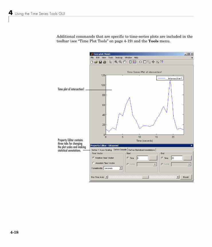
4 Using the Time Series Tools GUI
4-1
Additional commands that are specific to time-series plots are included in the toolbar (see “Time Plot Tools” on page 4-19) and the Tools menu.
���� ����������������%
&��������'��������������������������������������� ������ ���������!���������� ������������
8

Working with Time Plots
Time Plot ToolsThe Time Plot window contains several tools that are specific to time-series data. Click the button to enable the corresponding mode.
Data Analysis from a Time PlotThe following table summarizes the operations you can perform on an individual time series or on a time-series collection from a time plot.
These operations are available by right-clicking inside the time plot and selecting a command from the shortcut menu. Context-sensitive help provides detailed, on-the-spot instructions via the Help button in the Time Series Tools dialogs.
Time Plot Commands Specific to Time Series
Tool Button Description
Select Data — After enabling this mode, click and drag a rectangular region to select the data inside it.
Move Time Series — After enabling this mode, click and drag a time series to translate a time series on the plot and recalculate the data and time values.
Rescale Time Series — Click to rescale both axes of the time plot.
Select Interval — After enabling this mode, click and drag to select data within one or more time intervals.
4-19

4 Using the Time Series Tools GUI
4-2
Scaling the Time Plot GraphicallyTo identify important data features, it is often helpful to view the time plot at different scales. For data sets with fewer than 5000 points, the time-plot axes are scaled automatically to display the entire data set.
For performance reasons, larger data sets are shown in parts by displaying 5000 data points at a time. In this case, you can pan the data.
Summary of Time-Series Data Analysis Operations
Shortcut Menu Command
Description
Select Data Opens a dialog where you select data in a time plot by defining logical MATLAB expressions.
Remove Missing Data
Delete the times that contain missing data.
For time series with multiple data columns, the entire data sample is removed if any part of it contains missing data (see “Observation vs. Data Sample” on page 4-10).
Detrend Subtract a constant or a linear trend from the data.
Filter Smooth and shape the time-series data.
Resample Redefine a time series onto a new time vector by using interpolation.
Transform Algebraically
Create a new time series by algebraically manipulating existing time series.
Available only when you select an individual time series in the tree.
Descriptive Statistics
Get summary statistics of each time series.
0

Working with Time Plots
Note You can also scale axes in the Property Editor, where you have the additional option of setting axis limits by using events. To learn how to scale axes in the Property Editor, see “Scaling the Time Plot in the Property Editor” on page 4-22. For more information about defining events, see “Editing Data, Time, Attributes, and Events” on page 4-15.
Use the following procedures when graphically rescaling the time plot axes:
• “Zooming In on a Data Region” on page 4-21
• “Centering a Plot Region” on page 4-22
• “Restoring the Original Scale” on page 4-22
Zooming In on a Data RegionThe easiest way to rescale a time plot is by using the Zoom In command.
1 In the Time Plot window, click the Zoom In button in the toolbar.
This changes the mouse pointer to .
2 Do you want to zoom in only on a specific axis? By default, you zoom in on both axes.
- If yes, go to step 3.
- If no, go to step 4.
3 Right-click anywhere in the time plot and select one of the following:
- To zoom in on the horizontal axis only, select Zoom Options > Horizontal Zoom in the shortcut menu.
- To zoom in on the vertical axis only, select Zoom Options > Vertical Zoom in the shortcut menu.
4 Click the time plot region that you want to enlarge and center in the time plot.
4-21
4 Using the Time Series Tools GUI
4-2
Note To zoom out, right-click anywhere in the window and select Zoom Out in the shortcut menu.
Centering a Plot RegionThe simplest way to center a specific region of the plot without changing its magnification is by using the Pan command.
To center a specific plot region,
1 In the Time Plot window, click the Pan button in the toolbar.
This changes the pointer to .
2 Click anywhere on the plot and drag it to the desired position.
Restoring the Original ScaleRight-click anywhere inside the time plot and select Reset to Original View from the shortcut menu. This displays the full data set or the maximum window of 5000 points (whichever is larger).
Scaling the Time Plot in the Property EditorThe Property Editor for time-series plots is displayed at the bottom of the Time Plot window when you first create the plot.
This section describes how to perform the following operations in the Property Editor:
• “Scaling the Y Axis” on page 4-23
• “Scaling the Time Axis” on page 4-23
• “Displaying Summary Statistics on a Plot” on page 4-24
Tip If you close the Property Editor, you can reopen it by selecting View > Property Editor from the Time Plot menu bar. To display the Property Editor for a specific time-series plot, select it in the Plot Browser.
2

Working with Time Plots
Scaling the Y Axis
1 In the Time Plot Property Editor, select the Define Y Axes Scaling tab (if it is not already selected).
2 In the Ymin column, enter the minimum value of the Y axis. Press Enter.
3 In the Ymax column, enter the maximum value of the Y axis. Press Enter.
Tip To rescale the plot to display the full data set again, select auto in the Scaling column.
Scaling the Time AxisYou can scale the time axis in the Define Domain tab of the Time Plot Property Editor by specifying any of the following:
• The Start or End time, or both
• The Start or End event, or both
• A combination of a time and an event
If you have not defined any events for your time-series data, you can only specify the axis limits by time values. For more information about defining events, see “Editing Data, Time, Attributes, and Events” on page 4-15.
4-23

4 Using the Time Series Tools GUI
4-2
Note. If you are working with an Absolute time vector that uses calendar dates (nonempty StartDate property), you can display the time series on both an absolute and a relative time vector. However, if your time series uses a Relative time vector (empty StartDate property), you can only display the times series on a relative time vector. For more information about time series properties, see “Properties of a timeseries Object” on page 3-5.
Displaying Summary Statistics on a PlotThe following procedure describes how to display the mean, standard deviation (STD), and median of your time-series data on the time plot. You can specify the time interval for which these statistical measures are calculated.
Tip To view summary statistics for any time-series object that you imported or loaded into Time Series Tools, select that time series in the tree and choose Data > Descriptive Statistics.
1 In the Time Plot Property Editor, select the Define Statistical Annotations tab.
2 In the Show column, select the check box corresponding to each statistical measure you want to display on the plot:
- Mean
- STD
- Median
3 Do you want to change the time interval for any of the selected statistics? By default, the time interval is set to the entire length of the time vector.
- If yes, edit the Start Time or the End Time, or both, for each statistical measure.
If your time values are in terms of calendar dates, be careful to enter the time in the correct format.
- If no, you are done.
4

Selecting Time-Series Data
Selecting Time-Series DataBefore beginning data analysis, you might want to select the data on which to focus your analysis.
You can select the data in a specific time interval or within a specific range of values from a time plot:
• “Selecting Data by Using Rules” on page 4-26
Select data by creating logical expressions. Identify outliers and constant values.
• “Selecting Data Graphically” on page 4-27
Describes how to use the mouse to select data values or time intervals.
4-25

4 Using the Time Series Tools GUI
4-2
After you select the data, you can perform the following operations:
Selecting Data by Using RulesYou can specify data-selection rules in the Select Data Using Rules dialog, accessed from a time plot. For more information about creating time plots, see “Creating a Time Plot” on page 4-17.
To open the Select Data Using Rules dialog, right-click inside the time plot where you want to select data and choose Select Data from the shortcut menu.
Task Operation
Remove selected data from the time series
With multiple data columns in a single time-series object, removes the entire data sample at that time.
Right-click the selected data in the time plot and choose Remove Observations from the shortcut menu.
Remove all but the selected data from the time series
Right-click the selected data in the time plot and choose Keep Observations from the shortcut menu.
Replace the selected data with NaN (“Not-a-Number”) values
For more information, see “Handling Missing Data” on page 4-12.
Press the Delete key. Alternatively, right-click the selected data in the time plot and choose Replace with NaNs.
Then do one of the following to handle NaNs:
• Interpolate the missing values.
• Remove the data and the associated times from the time series.
6
Selecting Time-Series Data
You can define up to four kinds of data-selection conditions:
• Bounds — Upper and lower bounds for time and data values
• Outlier detection — Condition for detecting outliers, or data values that have a low likelihood of being consistent with the rest of the data
• MATLAB expression — A logical MATLAB expression that selects specific data values
• Flatline values — Condition for detecting flatlines, entered as the number of successive data points with a constant value
To learn what to do after you select the data, see “Selecting Time-Series Data” on page 4-25.
Selecting Data GraphicallyYou can select data in a time plot by using the mouse. For more information about creating time plots, see “Creating a Time Plot” on page 4-17.
You can select data using two modes:
• Data mode — Selects data values in a rectangular region
For more information, see “How to Select Data in a Rectangular Region on the Plot” on page 4-28.
• Time mode — Selects data values in a specific time interval
For more information, see “How to Select Data in a Time Interval” on page 4-28.
Tip To learn how you can select specific data values in a histogram plot, see “Select a Range of Data Values” on page 4-31.
4-27

4 Using the Time Series Tools GUI
4-2
How to Select Data in a Rectangular Region on the Plot
1 In the Time Plot window, click the Select Data button in the toolbar.
2 Click and drag a rectangular region on the plot that encloses the data you want to select.
The data values are selected when you release the mouse button.
3 Do you want to select another region?
- If yes, repeat step 2. This does not clear a previous selection.
- If no, continue as described in “Selecting Time-Series Data” on page 4-25.
How to Select Data in a Time Interval
1 In the Time Plot window, click the Select Time Interval(s) button in the toolbar.
2 Click the start of a region that encloses the time interval where you want to select data and drag it.
The selected time interval appears in a different color.
3 Do you want to select another time interval?
- If yes, repeat step 2.
- If no, continue as described in “Selecting Time-Series Data” on page 4-25.
8

Working with a Histogram
Working with a HistogramThe histogram plot shows the distribution of data values by counting the number of data values within a specific range of values and displaying each range as a rectangular bin. The heights of the bins represent the numbers of values that fall within each range.
You can use a histogram plot to select data values that fall in a specific range of values either to delete them, or to isolate them for analysis.
This section contains the following topics:
• “Creating a Histogram” on page 4-29
• “Modifying the Histogram in the Property Editor” on page 4-29
• “Select a Range of Data Values” on page 4-31
Note Time Series Tools generates a histogram plot of a time series by applyting the MATLAB hist function. You cannot save the plot from the plot window.
Creating a HistogramA convenient way to create a histogram is by dragging and dropping a time-series data node into the Histograms node in the Times Series Session tree.
The plot opens in a separate plot window that is similar to the standard MATLAB figure window, as described in the MATLAB documentation. Additional commands that are specific to time-series plots are included in the toolbar and the Tools menu.
Modifying the Histogram in the Property EditorThe Property Editor for histogram plots is displayed at the bottom of the Time-Series Viewer when you first create the plot.
4-29

4 Using the Time Series Tools GUI
4-3
This section describes how to perform the following operations in the Property Editor:
• “How to Scale the Y Axis” on page 4-30
• “How to Change the Data Bins” on page 4-31
• “How to Display Summary Statistics on the Plot” on page 4-31
Tip If you close the Property Editor, you can reopen it by selecting View > Property Editor from the Histogram window. To display the Property Editor for a specific histogram plot, select it in the Plot Browser. For example, select Histogram Plot in the Plot Browser to open the Property Editor for plot axes and statistics.
How to Scale the Y Axis
1 In the Histogram Property Editor, select the Define Y Axes Scaling tab (if it is not already selected).
2 In the Ymin column, enter the minimum value of the Y axis. Press Enter.
3 In the Ymax column, enter the maximum value of the Y axis. Press Enter.
Tip To rescale the plot to display the full data set again, select auto in the Scaling column.
0

Working with a Histogram
How to Change the Data BinsYou can change the bin size by specifying either uniform bins or custom bins. By default, the data is distributed into 50 bins.
1 In the Histogram Property Editor, select the Define Bins tab.
2 Do you want uniform bins?
- If yes, select Uniform centers and edit the Number of bins. You are done.
- If no, go to step 3.
3 To specify custom bins, select Custom centers and enter the vector of bin centers. Use MATLAB syntax for entering a vector, but omit the square brackets around the vector.
For example, enter 1:10 to specify the vector [1, 2, 3, 4, 5, 6, 7, 8, 9, 10].
How to Display Summary Statistics on the PlotThe following procedure describes how to display the mean and median of your time-series data on the histogram:
1 In the Histogram Property Editor, select the Define Statistical Annotations tab.
2 In the Show column, select the check box corresponding to each statistical measure you want to display on the plot:
- Mean- Median
Select a Range of Data Values
1 In the Histogram window, click the Select Y Range Interval(s) button in the toolbar.
2 Click the region aligned with the start of the data interval and drag to select the data interval.
The selected data interval displays the data in a different color.
4-31

4 Using the Time Series Tools GUI
4-3
3 Do you want to select another time interval?
- If yes, repeat step 2.
- If no, go to step 4.
4 Do you want to remove the data values in the selected region? This also removes the corresponding times from the time series.
- If yes, right-click the selected data in the plot and choose Remove Selection from the shortcut menu. You are done.
- If no, go to step 5.
5 Do you want to replace the selected data with NaN values?
- If yes, press Delete. To learn how to handle NaN-tagged data, see “Handling Missing Data” on page 4-12.
- If no, you are done.
2

Working with a Spectral Plot
Working with a Spectral PlotYou use a spectral plot (or periodogram) of time-series data to gain insight into the frequencies of the periodic variations in the data. The periodogram is particularly useful for picking out periodic components in the presence of noise; a peak in the periodogram indicates an important contribution to variance frequencies near the value that corresponds to the peak.
The periodogram is the unbiased estimate of the power spectral density of time-series data, calculated as the scaled absolute value of the (FFT)2 of the time series. The corresponding frequency vector is computed in cycles per unit time and has the same length as the power vector.
The periodogram is scaled so that the variance is equal to the mean of the periodogram. To learn how to view the variance in a specific frequency range, see “How to Display the Variance on the Plot” on page 4-36.
This section contains the following topics:
• “Creating a Periodogram” on page 4-33
• “Modifying the Periodogram in the Property Editor” on page 4-34
• “How to Filter the Data in a Frequency Range” on page 4-38
Note You cannot save the plot from the plot window.
Creating a PeriodogramA convenient way to create a spectral plot is by dragging and dropping a time-series data node into the Spectral Plots node in the Times Series Session tree.
The plot opens in a separate plot window that is similar to the standard MATLAB figure window, as described in the MATLAB documentation. Additional commands that are specific to time-series plots are included in the toolbar and the Tools menu.
4-33
4 Using the Time Series Tools GUI
4-3
Modifying the Periodogram in the Property EditorThe Property Editor for spectral plots is displayed at the bottom of the Histogram plot when you first create the plot.
4

Working with a Spectral Plot
This section describes how to perform the following operations in the Property Editor:
• “How to Scale the Y Axis” on page 4-35
• “How to Scale the Frequency Axis” on page 4-36
• “How to Display the Variance on the Plot” on page 4-36
Tip If you close the Property Editor, you can reopen it by selecting View > Property Editor from the Time-Series Viewer menu bar. To display the Property Editor for a specific histogram plot, select it in the Plot Browser. For example, select Spectral Plot in the Plot Browser to open the Property Editor for plot axes and statistics.
How to Scale the Y Axis
1 In the Spectral Plot Property Editor, select the Define Y Axes Scaling tab (if it is not already selected).
2 In the Ymin column, enter the minimum value of the Y axis. Press Enter.
3 In the Ymax column, enter the maximum value of the Y axis. Press Enter.
Tip To rescale the plot to display the full data set again, select auto in the Scaling column.
4-35

4 Using the Time Series Tools GUI
4-3
How to Scale the Frequency Axis
1 In the Spectral Plot Property Editor, select the Define Frequency Vector tab.
2 Do you want to set a different start frequency?
- If yes, enter a new value in the Start frequency field. Press Enter and go to step 3.
- If no, go to step 3.
3 Do you want to set a different end frequency?
- If yes, enter a new value in the End frequency field. Press Enter and go to step 4.
- If no, go to step 4.
4 Do you want to change the frequency units?
- If yes, select the units from the Units list. Press Enter.
- If no, you are done.
How to Display the Variance on the PlotThe periodogram is scaled so that the variance is equal to the mean of the periodogram.
To get a quantitative estimate of how much variation occurs in a specific frequency range, you set the frequency interval on the plot and display a tooltip with the percent of the total variance in that interval.
To display the variance on the plot,
1 In the Spectral Plot Property Editor, select the Define Statistical Annotations tab.
2 In the Show column, select the Variance check box.
This adds a horizontal line to the graph to indicate the variance.
6

Working with a Spectral Plot
3 Do you want to change the Low limit of the frequency range?
- If yes, double-click the Low limit field to make it editable and type the lowest frequency. Press Enter.
- If no, go to step 4.
4 Do you want to change the High limit of the frequency range?
- If yes, double-click the High limit field to make it editable and type the highest frequency. Press Enter.
- If no, go to step 5.
5 To display a tooltip with the percent of the total variance in the interval, click or hover over the corner of the rectangle that marks the frequency range. The percent value is given by the Variance fraction in the tooltip.
4-37

4 Using the Time Series Tools GUI
4-3
How to Filter the Data in a Frequency RangeYou can use the spectral plot to apply an ideal pass or stop filter to the data. You use the ideal notch (stop) filter when you want to attenuate the variations in the data for a specific frequency range. Alternatively, you use the ideal pass filter to allow only the variations in a specific frequency range.
These filters are “ideal” in the sense that they are not realizable; an ideal filter is noncausal and the ends of the filter amplitude are perfectly flat in the frequency domain.
To apply the ideal filter in the periodogram,
1 In the Spectral Plot window, click the Select Frequency Interval(s) button in the toolbar.
2 Click the starting frequency and drag a region that encloses the frequency interval.
The selected time interval appears in a different color.
3 Do you want to select another frequency interval?
- If yes, repeat step 2.
- If no, go to step 4.
4 Right-click anywhere on the plot and select one of the following from the shortcut menu:
- To allow only the variations in the selected frequency range, select Pass.
- To remove the variations in the selected frequency range, select Notch.
8

Working with a Correlogram
Working with a CorrelogramThe autocorrelation function is a major diagnostic tool for analyzing time series in the time domain. You use the autocorrelation plot, or a correlogram, to gain insight into the correlation between observations at different distances apart (lags) to better understand the evolution of a process through time.
A correlogram plot is not useful when the data contains a trend; data at all lags will appear to be correlated because an observation on one side of the mean tends to be followed by a large number of observations on the same side of the mean. You must remove any trend in the data before you create a correlogram. For more information about accessing detrending functionality, see “Time-Series Analysis Operations” on page 4-5.
What Is Plotted in the CorrelogramThe correlogram is a plot of correlation coefficients between observations that are k steps apart.
The correlation coefficients are given by
where is an observation at time t, and the overall mean is
Note k is also called the lag between observations.
rk
rk
xt x–( ) xt k+ x–( )
t 1=
N
∑
xt x–( )2
t 1=
N
∑
--------------------------------------------------------=
xt
x xt N⁄
t 1=
N
∑=
4-39

4 Using the Time Series Tools GUI
4-4
Creating a CorrelogramA convenient way to create a spectral plot is by dragging and dropping a time-series data node into the Correlations node in the Times Series Session tree.
The plot opens in a separate plot window that is similar to the standard MATLAB figure window, as described in the MATLAB documentation. Additional commands that are specific to time-series plots are included in the toolbar and the Tools menu.
1 Click and hold down the mouse button on the name of the time-series data in the Time Series node.
2 Drag the data into Correlations in the Views node.
3 In the Data Explorer, right-click the new plot in the Views node and select Rename from the shortcut menu.
4 Enter the name of the plot and click OK.
Note You cannot save the plot from the plot window.
Modifying the Correlogram in the Property EditorThe Property Editor for correlogram plots is displayed at the bottom of the Correlation plot when you first create the plot.
This section describes how to perform the following operations in the Property Editor:
• “How to Scale the Y Axis” on page 4-41
• “How to Modify the Lag Range” on page 4-42
0

Working with a Correlogram
Tip If you close the Property Editor, you can reopen it by selecting View > Property Editor from the Time-Series Viewer menu bar. To display the Property Editor for a specific correlogram plot, select it in the Plot Browser. For example, select Time Series Correlation in the Plot Browser to open the Property Editor.
How to Scale the Y Axis
Note The possible values of autocorrelation coefficients range between -1 and +1.
1 In the Correlogram Property Editor, select the Define Y Axes Scaling tab (if it is not already selected).
2 In the Ymin column, enter the minimum value of the Y axis. Press Enter.
3 In the Ymax column, enter the maximum value of the Y axis. Press Enter.
Tip To rescale the plot to display the full data set again, select auto in the Scaling column.
4-41

4 Using the Time Series Tools GUI
4-4
How to Modify the Lag Range
1 In the Correlogram Property Editor, select the Define Lags tab.
2 Do you want to modify the smallest lag?
- If yes, enter a new value in the From field. Press Enter and go to step 3.
- If no, go to step 3.
3 Do you want to modify the largest lag?
- If yes, enter a new value in the To field. Press Enter.
- If no, you are done.
2

Comparing Time Series
Comparing Time SeriesTime Series Tools enables you to compare two sets of data by
• “Creating an XY Plot” on page 4-43
• “Creating a Cross-Correlation Plot” on page 4-44
Note You cannot save the plot from the plot window.
Creating an XY PlotAn XY plot plots data values from two different time series. Any relationship between the two time series is evident from a pattern on the plot.
Note For you to generate an XY plot, both time series must have the same time vectors.
How to Create an XY PlotTo create an XY plot,
1 Select a time series in the Time Series Session tree.
2 In the Plot time series area, select Create new. Then choose XY Plots from the list.
3 In the named field, enter the plot name.
4 Click Display.
A blank plot appears in the XY Plot window. To complete the plot you must add a second time series to the plot.
To add a second time-series object to the plot,
1 Select another time-series object in the Time Series Session tree.
4-43

4 Using the Time Series Tools GUI
4-4
2 In the Display Time Series section, select Add to existing plot.
3 In the list, select the XY plot created in step 3 of the above procedure and click Display.
Tip You can also create an XY plot by dragging a time series onto XY Plots in the Time Series Session tree, and then dragging another time series onto the same XY Plots node.
Interpreting XY PlotsThe XY plot is useful for determining relationships between two sets of data. For example, when the points of the XY plot form a straight line, there is a linear relationship between the two data sets.
When you are comparing two time series such that each has a single column of data, the XY plot contains a single set of axes.
Each point on the plot represents a single data value from each data set. Both data values are taken from the same position in the column of data; i.e., the third data point from one data set is plotted against the third data point from the other data set. The plot does not show time information.
When you are comparing two time series that contain several columns of data, the XY plot shows a grid of axes. Each axis displays an XY plot between two corresponding columns of data.
Creating a Cross-Correlation PlotCross-correlation is a measure of the degree of the linear relationship between two data sets. It is similar to autocorrelation except that it compares values in two different data sets instead of comparing different values within the same data set. For more information about correlation coefficients, see “Correlation Coefficients” on page 1-23.
How to Create a Cross-Correlation PlotTo create a cross-correlation plot,
1 Select a time series in the Time Series Session tree.
4

Comparing Time Series
2 In the Plot time series area, select Create new. Then choose Correlations from the list.
3 In the named field, enter the plot name.
4 Click Display.
A blank plot appears in the Correlation Plot window. To complete the plot you must add a second time series to the plot.
To add a second time-series object to the plot,
1 Select another time-series object in the Time Series Session tree.
2 In the Display Time Series section, select Add to existing plot.
3 In the list, select the correlation plot created in step 3 of the above procedure and click Display.
This displays the cross-correlation plot of the two time-series objects.
Tip You can also create a cross-correlation plot by dragging a time series onto Correlations in the Time Series Session tree, and then dragging another time series onto the same Correlations node.
Interpreting Cross-Correlation PlotsThe cross-correlation is computed at several different lags. This means that the data sets are translated with respect to each other before the cross-correlation is plotted.
A cross-correlation plot of two single-column time-series objects shows the degree of linear relationship between the data values. The following table
4-45

4 Using the Time Series Tools GUI
4-4
connects the cross-correlation value to the degree of relationship between the data sets:
A correlation plot of two time series with multiple data columns contains a grid of axes, where each plot shows the cross-correlations between corresponding data columns in the time series.
The number of axes in the plot is equal to the number of columns of data in the first time series multiplied by the number of columns of data in the second time series.
Interpreting Cross-Correlation Values
Cross-Correlation Value Is Close To
Meaning
1 A strong linear relationship between the data values: An increase in one data set corresponds to an increase in the other data set.
-1 A strong anticorrelation between the data values: A decrease in the data values of one data set corresponds to a decrease in the values of the other data set.
0 The variations in the data show no relationships.
6

Example — Analyzing Time-Series Data with Time Series Tools
Example — Analyzing Time-Series Data with Time Series Tools
This example illustrates how to perform the following tasks in Time Series Tools:
• “Loading Data into the MATLAB Workspace” on page 4-47
• “Starting Time Series Tools” on page 4-47
• “Importing Data into Time Series Tools” on page 4-47
• “Creating a Time Plot” on page 4-50
• “Resampling Time Series on a New Time Vector” on page 4-55
• “Comparing Data on an XY Plot” on page 4-57
Loading Data into the MATLAB WorkspaceType the following command to load the data set with hourly traffic counts at three road intersections in the same town, collected over a 24-hour period. For information about the data sets in this example, see “About the Example Data” on page 3-22.
load count.dat
This adds the variable count to the MATLAB workspace.
Starting Time Series ToolsTo start Time Series Tools, type
tstool
This opens the Time Series Tools window. For more information about the graphical user interface (GUI), see “Time Series Tools Window” on page 4-3.
Importing Data into Time Series ToolsThis portion of the example illustrates how to create three time-series objects from the 24-by-3 count array you loaded into the MATLAB workspace.
4-47

4 Using the Time Series Tools GUI
4-4
Note To get help on a specific field in the Import Wizard, right-click the field label and select What’s This from the shortcut menu.
1 In Time Series Tools, select File > Import > Raw Data. This opens the Import Wizard.
2 In the Import from list, select MATLAB workspace and click Next.
3 In Step 2 of the Import Wizard, select the count variable. The Import Wizard infers from the data that it is arranged by columns and imports the full 24-by-3 array.
8

Example — Analyzing Time-Series Data with Time Series Tools
4 In the Specify Time Vector area, select hours from the Units list. The Import Wizard has already specified the remaining options to define a uniformly spaced time vector with a length of 24 and an interval of 1.
5 Click Next.
6 In Step 3 of the Import Wizard, select Create several time series using: common name+number and Enter common name: intersection.
7 Click Finish. This adds three time series to the Time Series Session tree, named intersection1, intersection2, and intersection3.
(������������������������������������������������
4-49

4 Using the Time Series Tools GUI
4-5
Creating a Time PlotTo explore the data, you can create a time plot of the three time series.
1 In the Time Series Session tree, drag and drop the intersection1 time series into the Time Plots node. This creates a time plot in a new window with the default name View1.
���� ����������������%
&��������'��������������������������������������� ������ ���������!���������� ������������
0

Example — Analyzing Time-Series Data with Time Series Tools
2 In the Time Series Session tree, drag and drop the intersection2 and intersection3 time series into the View1 node to add them to the plot.
4-51
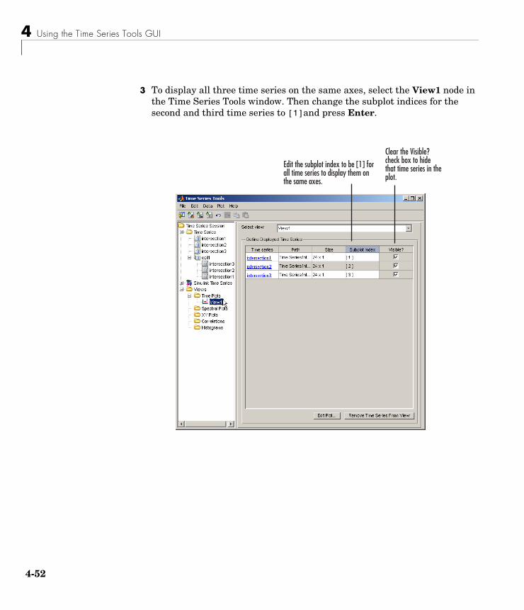
4 Using the Time Series Tools GUI
4-5
3 To display all three time series on the same axes, select the View1 node in the Time Series Tools window. Then change the subplot indices for the second and third time series to [1]and press Enter.
'����������� ��������������)%*����� ����������������� ������������������������
� ����������� �+����!�������������������������������� ���
2

Example — Analyzing Time-Series Data with Time Series Tools
This groups the plots as shown below:
4-53

4 Using the Time Series Tools GUI
4-5
4 To change the appearance of the time series in the plot, select Plot > Set Line Properties. This opens the Line Styles dialog.
� �!������������������������������� �������� ��$����!��$��� ������ ����������������������������
�� ��������������������� ��������������� ���������� ������ ���
4

Example — Analyzing Time-Series Data with Time Series Tools
The plot now looks like this:
Resampling Time Series on a New Time VectorYou can cast two of the three time series onto a new time vector with samples every half hour, rather than every hour. The new data points are calculated by using the interpolation method you associated with the time series (see “Editing Data, Time, Attributes, and Events” on page 4-15).
4-55

4 Using the Time Series Tools GUI
4-5
First, resample the time series intersection1:
1 In the Time Series Session tree, select the time series intersection1.
2 Select Data > Resample. This opens the Resample Data dialog.
3 Select the Uniform time vector with time interval option, and specify the time interval to be 0.5 hour. Click OK.
6

Example — Analyzing Time-Series Data with Time Series Tools
You can resample intersection2 a different way by
• Creating a common vector for intersection1 and intersection2 by taking the union of their time vector
• Resampling intersection2 on the common time vector
To resample intersection2,
1 In the time plot you created in “Creating a Time Plot” on page 4-50, right-click and select Data > Resample from the shortcut menu. This opens the Resample Data dialog.
2 In the Resample Data dialog, clear the check box to the left of intersection3 to exclude it from resampling.
3 Select Union of time vectors on the interval where they overlap. Click OK.
• To verify that intersection2 has been resampled, select it in the Time Series Session tree and examine the data table. The union of the time vectors is the same as the time vector for intersection1 after it was resampled at half-hour intervals.
Comparing Data on an XY PlotThe XY plot is useful for determining relationships between two sets of data. For example, when the points of the XY plot form a straight line, there is a linear relationship between the two data sets.
To compare intersection1 and intersection2 on an XY plot,
1 In the Time Series Session tree, drag and drop the intersection1 time series into the XY Plots node. This creates a new plot node with the default name View2.
4-57

4 Using the Time Series Tools GUI
4-5
2 Drag and drop the intersection2 time series into the View2 node. This creates the following XY plot.
3 To show the best-fit line on the XY plot, select the Define Statistical Annotations tab in the Property Editor in the XY Plot window.
Note that this XY plot shows a strong linear correlation between the two data sets.
8

Example — Analyzing Time-Series Data with Time Series Tools
4 Select the Best fit line check box. This adds a best-fit line to the plot.
4-59

4 Using the Time Series Tools GUI
4-6
0
Index
BBasic Fitting tool 2-4
example 2-9
Cconfidence bounds 2-27correlation coefficients 1-23correlogram 4-39covariance 1-22cross-correlation plot 4-44curve fitting
See data fitting
Ddata analysis
MATLAB functions 1-2MATLAB tools 1-3plot data 1-6related products 1-3vector and matrix data 1-3
data filteringSee filtering
data fitting 2-1at the command line 2-17Basic Fitting tool 2-4confidence bounds 2-27example using command line 2-23exponential 2-26multiple regression 2-21nonpolynomial 2-19polynomial 2-23residuals 2-3
data sample 3-3data statistics
formatting plots of 1-19in plot legend 1-19
Data Statistics tool 1-17example 1-18interface 1-18saving to workspace 1-21
descriptive statistics 1-15detrending data 1-30difference equations 1-25discrete filter 1-27discrete Fourier transform
See Fourier transforms
Eexponential data fitting 2-26exporting data 1-5
Ffast Fourier transform
See Fourier transformsfiltering
detrending data 1-30difference equations 1-25discrete filter 1-27filter function 1-25moving average 1-26
finite differences 1-24Fourier analysis 1-31
calculating sunspot periodicity 1-33Fourier transforms
Index-1

Index
Ind
calculating the FFT 1-32performance of calculation 1-38phase and magnitude 1-36
function M-files 1-2functions
for timeseries object 3-11for tscollection object 3-20
Ggoodness of fit 2-3
Hhistogram 4-29
Iimporting data 1-5
into Time Series Tools 4-9interpolation
missing data 1-11isnan function 1-10
Lload function 1-6
Mmagnitude of Fourier transform 1-36maximum 1-15mean 1-15median 1-15minimum 1-15missing data
about 1-9handling in Time Series Tools 4-12
ex-2
interpolate 1-11propagation through calculations 1-9removing 1-10representing by NaNs 1-9
mode 1-15moving average filter 1-26multiple regression 2-21
NNaNs
propagation in calculations 1-9removing from data 1-10
nonpolynomial fit 2-19
Oobservation 3-3outliers
removing from data 1-13
Pperiodogram 4-33phase of Fourier transform 1-36plotting data
correlogram in Time Series Tools 4-39cross-correlation plot in Time Series Tools 4-44histogram in Time Series Tools 4-29in MATLAB 1-6periodogram in Time Series Tools 4-33time plot in Time Series Tools 4-17XY plot in Time Series Tools 4-43
plotting tools 1-3polynomial regression 2-23

Index
propertiesof timeseries object 3-5of tscollection object 3-19
Rregression 2-1
multiple 2-21nonpolynomial 2-19polynomial 2-17
residuals 2-3
Ssample 3-3Simulink logged-data signals 4-9spectral plot 4-33standard deviation 1-15statistics
calculating 1-15Data Statistics tool 1-17format on plot 1-19formatting plots of 1-19removing NaNs 1-10removing outliers 1-13saving to workspace 1-21
sunspot periodicitycalculating using Fourier transforms 1-33
Ttime plot 4-17Time Series Tools
correlogram 4-39cross-correlation plot 4-44example 4-47GUI 4-1
histogram 4-29import data 4-9importing Simulink logged signal 4-9periodogram 4-33time plot 4-17XY plot 4-43
time-series analysiscommand-line API 3-1comparing time series 4-43data sample 3-3example for command line 3-22example for Time Series Tools 4-47observation 3-3Time Series Tools 4-1
timeseries objectcreating 3-3functions 3-11properties 3-5
toolsBasic Fitting 2-4Data Statistics 1-17plotting 1-3summary 1-3Time Series Tools 4-1
tscollection objectcreating 3-17functions 3-20properties 3-19
Vvariance 1-15
XXY plot 4-43
Index-3