
matlab pde solving.pdf
290
Computation Visualization Programming User’s Guide Version 1 Partial Differential Equation T oolbox COMSOL AB
-
Upload
praveenrajj -
Category
Documents
-
view
235 -
download
0
Transcript of matlab pde solving.pdf
8/21/2019 matlab pde solving.pdf
http://slidepdf.com/reader/full/matlab-pde-solvingpdf 1/290
Computation
Visualization
Programming
User’s GuideVersion 1
Partial DifferentialEquation Toolbox
COMSOL AB
8/21/2019 matlab pde solving.pdf
http://slidepdf.com/reader/full/matlab-pde-solvingpdf 2/290
How to Contact The MathWorks:
www.mathworks.com Webcomp.soft-sys.matlab Newsgroup
[email protected] Technical [email protected] Product enhancement [email protected] Bug reports
[email protected] Documentation error [email protected] Order status, license renewals, [email protected] Sales, pricing, and general information
508-647-7000 Phone
508-647-7001 Fax
The MathWorks, Inc. Mail3 Apple Hill DriveNatick, MA 01760-2098
For contact information about worldwide offices, see the MathWorks Web site.
Partial Differential Equation Toolbox User’s Guide
© COPYRIGHT 1995 - 2002 by The MathWorks, Inc.
The software described in this document is furnished under a license agreement. The software may beused or copied only under the terms of the license agreement. No part of this manual may be photocopiedor reproduced in any form without prior written consent from The MathWorks, Inc.
U.S. GOVERNMENT: If Licensee is acquiring the Programs on behalf of any unit or agency of the U.S.Government, the following shall apply: (a) For units of the Department of Defense: the Government shallhave only the rights specified in the license under which the commercial computer software or commercialsoftware documentation was obtained, as set forth in subparagraph (a) of the Rights in CommercialComputer Software or Commercial Software Documentation Clause at DFARS 227.7202-3, therefore therights set forth herein shall apply; and (b) For any other unit or agency: NOTICE: Notwithstanding anyother lease or license agreement that may pertain to, or accompany the delivery of, the computer softwareand accompanying documentation, the rights of the Government regarding its use, reproduction, anddisclosure are as set forth in Clause 52.227-19 (c)(2) of the FAR.MATLAB, Simulink, Stateflow, Handle Graphics, and Real-Time Workshop are registered trademarks,and TargetBox is a trademark of The MathWorks, Inc.
Other product or brand names are trademarks or registered trademarks of their respective holders.
Printing History: August 1995 First printingFebruary 1996 ReprintJuly 2002 Online only New for Version 1.0.4 (Release 13)
8/21/2019 matlab pde solving.pdf
http://slidepdf.com/reader/full/matlab-pde-solvingpdf 3/290
i
Contents
1
Tutorial
Introduction . . . . . . . . . . . . . . . . . . . . . . . . . . . . . . . . . . . . . . . . . 1-2
Can I Use the PDE Toolbox? . . . . . . . . . . . . . . . . . . . . . . . . . . . . 1-2
What Problems Can I Solve? . . . . . . . . . . . . . . . . . . . . . . . . . . . . 1-3
In Which Areas Can the Toolbox Be Used? . . . . . . . . . . . . . . . . 1-5
How Do I Define a PDE Problem? . . . . . . . . . . . . . . . . . . . . . . . 1-5
How Can I Solve a PDE Problem? . . . . . . . . . . . . . . . . . . . . . . . 1-6Can I Use the Toolbox for Nonstandard Problems? . . . . . . . . . 1-6
How Can I Visualize My Results? . . . . . . . . . . . . . . . . . . . . . . . 1-7
Are There Any Applications Already Implemented? . . . . . . . . . 1-7
Can I Extend the Functionality of the Toolbox? . . . . . . . . . . . . 1-8
How Can I Solve 3-D Problems by 2-D Models? . . . . . . . . . . . . 1-8
Getting Started . . . . . . . . . . . . . . . . . . . . . . . . . . . . . . . . . . . . . . . 1-9
Basics of the Finite Element Method . . . . . . . . . . . . . . . . . . . 1-20
Using the PDE Toolbox Graphical User Interface . . . . . . . 1-25
The Menus . . . . . . . . . . . . . . . . . . . . . . . . . . . . . . . . . . . . . . . . . 1-26
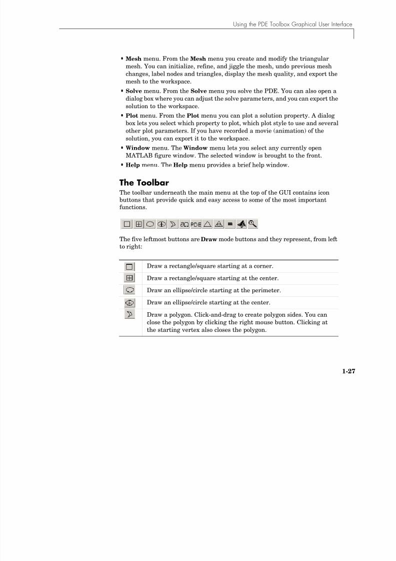
The Toolbar . . . . . . . . . . . . . . . . . . . . . . . . . . . . . . . . . . . . . . . . 1-27
The GUI Modes . . . . . . . . . . . . . . . . . . . . . . . . . . . . . . . . . . . . . 1-28
The CSG Model and the Set Formula . . . . . . . . . . . . . . . . . . . 1-30Creating Rounded Corners . . . . . . . . . . . . . . . . . . . . . . . . . . . . 1-31
Suggested Modeling Method . . . . . . . . . . . . . . . . . . . . . . . . . . . 1-34
Object Selection Methods . . . . . . . . . . . . . . . . . . . . . . . . . . . . . 1-38
Display Additional Information . . . . . . . . . . . . . . . . . . . . . . . . 1-38
Entering Parameter Values as MATLAB Expressions . . . . . . 1-39
Using Earlier Version PDE Toolbox Model M-Files . . . . . . . . 1-39
Using Command-Line Functions . . . . . . . . . . . . . . . . . . . . . . 1-40
Data Structures and Utility Functions . . . . . . . . . . . . . . . . . . 1-40
Hints and Suggestions for Using Command-Line Functions . 1-44
8/21/2019 matlab pde solving.pdf
http://slidepdf.com/reader/full/matlab-pde-solvingpdf 4/290
ii Contents
2
Examples
Examples of Elliptic Problems . . . . . . . . . . . . . . . . . . . . . . . . . . 2-2
Poisson’s Equation on Unit Disk . . . . . . . . . . . . . . . . . . . . . . . . . 2-2
A Scattering Problem . . . . . . . . . . . . . . . . . . . . . . . . . . . . . . . . . . 2-7
A Minimal Surface Problem . . . . . . . . . . . . . . . . . . . . . . . . . . . 2-11
Domain Decomposition . . . . . . . . . . . . . . . . . . . . . . . . . . . . . . . 2-13
Examples of Parabolic Problems . . . . . . . . . . . . . . . . . . . . . . 2-17
The Heat Equation: A Heated Metal Block . . . . . . . . . . . . . . . 2-17
Heat Distribution in Radioactive Rod . . . . . . . . . . . . . . . . . . . . 2-21
Example of a Hyperbolic Problem . . . . . . . . . . . . . . . . . . . . . 2-23
The Wave Equation . . . . . . . . . . . . . . . . . . . . . . . . . . . . . . . . . . 2-23
Examples of Eigenvalue Problems . . . . . . . . . . . . . . . . . . . . . 2-28
Eigenvalues and Eigenfunctions for the L-Shaped Membrane 2-28
L-Shaped Membrane with Rounded Corner . . . . . . . . . . . . . . . 2-32Eigenvalues and Eigenmodes of a Square . . . . . . . . . . . . . . . . 2-34
Application Modes . . . . . . . . . . . . . . . . . . . . . . . . . . . . . . . . . . . 2-37
The Application Modes and the GUI . . . . . . . . . . . . . . . . . . . . . 2-37
Structural Mechanics — Plane Stress . . . . . . . . . . . . . . . . . . . 2-38
Structural Mechanics — Plane Strain . . . . . . . . . . . . . . . . . . . 2-44
Electrostatics . . . . . . . . . . . . . . . . . . . . . . . . . . . . . . . . . . . . . . . 2-44
Magnetostatics . . . . . . . . . . . . . . . . . . . . . . . . . . . . . . . . . . . . . . 2-47
AC Power Electromagnetics . . . . . . . . . . . . . . . . . . . . . . . . . . . 2-53
Conductive Media DC . . . . . . . . . . . . . . . . . . . . . . . . . . . . . . . . 2-59
Heat Transfer . . . . . . . . . . . . . . . . . . . . . . . . . . . . . . . . . . . . . . . 2-62
Diffusion . . . . . . . . . . . . . . . . . . . . . . . . . . . . . . . . . . . . . . . . . . . 2-65
References . . . . . . . . . . . . . . . . . . . . . . . . . . . . . . . . . . . . . . . . . . 2-66
8/21/2019 matlab pde solving.pdf
http://slidepdf.com/reader/full/matlab-pde-solvingpdf 5/290
iii
3
The Graphical User Interface
PDE Toolbox Menus . . . . . . . . . . . . . . . . . . . . . . . . . . . . . . . . . . . 3-2
File Menu . . . . . . . . . . . . . . . . . . . . . . . . . . . . . . . . . . . . . . . . . . . 3-2
Edit Menu . . . . . . . . . . . . . . . . . . . . . . . . . . . . . . . . . . . . . . . . . . . 3-5
Options Menu . . . . . . . . . . . . . . . . . . . . . . . . . . . . . . . . . . . . . . . . 3-7
Draw Menu . . . . . . . . . . . . . . . . . . . . . . . . . . . . . . . . . . . . . . . . . 3-10
Boundary Menu . . . . . . . . . . . . . . . . . . . . . . . . . . . . . . . . . . . . . 3-13
PDE Menu . . . . . . . . . . . . . . . . . . . . . . . . . . . . . . . . . . . . . . . . . 3-16
Mesh Menu . . . . . . . . . . . . . . . . . . . . . . . . . . . . . . . . . . . . . . . . . 3-20
Solve Menu . . . . . . . . . . . . . . . . . . . . . . . . . . . . . . . . . . . . . . . . . 3-23Plot Menu . . . . . . . . . . . . . . . . . . . . . . . . . . . . . . . . . . . . . . . . . . 3-28
Window Menu . . . . . . . . . . . . . . . . . . . . . . . . . . . . . . . . . . . . . . 3-35
Help Menu . . . . . . . . . . . . . . . . . . . . . . . . . . . . . . . . . . . . . . . . . 3-35
The Toolbar . . . . . . . . . . . . . . . . . . . . . . . . . . . . . . . . . . . . . . . . . 3-36
4
The Finite Element Method
The Elliptic Equation . . . . . . . . . . . . . . . . . . . . . . . . . . . . . . . . . . 4-2
The Elliptic System . . . . . . . . . . . . . . . . . . . . . . . . . . . . . . . . . . . 4-9
The Parabolic Equation . . . . . . . . . . . . . . . . . . . . . . . . . . . . . . 4-12
The Hyperbolic Equation . . . . . . . . . . . . . . . . . . . . . . . . . . . . . 4-15
The Eigenvalue Equation . . . . . . . . . . . . . . . . . . . . . . . . . . . . . 4-16
Nonlinear Equations . . . . . . . . . . . . . . . . . . . . . . . . . . . . . . . . . 4-20
Adaptive Mesh Refinement . . . . . . . . . . . . . . . . . . . . . . . . . . . 4-25
The Error Indicator Function . . . . . . . . . . . . . . . . . . . . . . . . . . 4-25
The Mesh Refiner . . . . . . . . . . . . . . . . . . . . . . . . . . . . . . . . . . . . 4-26
The Termination Criteria . . . . . . . . . . . . . . . . . . . . . . . . . . . . . 4-27
8/21/2019 matlab pde solving.pdf
http://slidepdf.com/reader/full/matlab-pde-solvingpdf 6/290
iv Contents
Fast Solution of Poisson’s Equation . . . . . . . . . . . . . . . . . . . . 4-28
References . . . . . . . . . . . . . . . . . . . . . . . . . . . . . . . . . . . . . . . . . . 4-30
5
Function Reference
Functions — By Category . . . . . . . . . . . . . . . . . . . . . . . . . . . . . . 5-2
PDE Algorithms . . . . . . . . . . . . . . . . . . . . . . . . . . . . . . . . . . . . . . 5-3User Interface Algorithms . . . . . . . . . . . . . . . . . . . . . . . . . . . . . . 5-3
Geometry Algorithms . . . . . . . . . . . . . . . . . . . . . . . . . . . . . . . . . . 5-3
Plot Functions . . . . . . . . . . . . . . . . . . . . . . . . . . . . . . . . . . . . . . . 5-5
Utility Algorithms . . . . . . . . . . . . . . . . . . . . . . . . . . . . . . . . . . . . 5-5
User Defined Algorithms . . . . . . . . . . . . . . . . . . . . . . . . . . . . . . . 5-6
Demonstration Programs . . . . . . . . . . . . . . . . . . . . . . . . . . . . . . 5-6
Functions — Alphabetical List . . . . . . . . . . . . . . . . . . . . . . . . . 5-7
Index
8/21/2019 matlab pde solving.pdf
http://slidepdf.com/reader/full/matlab-pde-solvingpdf 7/290
1
Tutorial
The Partial Differential Equation (PDE) Toolbox provides a powerful and flexible environment for thestudy and solution of partial differential equations in two space dimensions and time. The equationsare discretized by the Finite Element Method (FEM).
Introduction (p. 1-2) An overview of the features, functions, and uses of thePDE Toolbox.
Getting Started (p. 1-9) Instruction on how to use the GUI to solve a PDE
problem.Basics of the Finite Element Method(p. 1-20)
Description of the use of the Finite Element Method(FEM) to approximate a piecewise linear function andthe use of FEM techniques to solve more generalproblems.
Using the PDE Toolbox Graphical UserInterface (p. 1-25)
A detailed description of the use of the PDE ToolboxGUI.
Using Command-Line Functions (p. 1-40) Instruction on the use of command-line functions as analternative to the GUI.

8/21/2019 matlab pde solving.pdf
http://slidepdf.com/reader/full/matlab-pde-solvingpdf 8/290
1 Tutorial
1-2
IntroductionThe objectives of the PDE Toolbox are to provide you with tools that
Define a PDE problem, e.g., define 2-D regions, boundary conditions, andPDE coefficients.
•Numerically solve the PDE problem, e.g., generate unstructured meshes,discretize the equations, and produce an approximation to the solution.
• Visualize the results.
Can I Use the PDE Toolbox?The PDE Toolbox is designed for both beginners and advanced users.
The minimal requirement is that you can formulate a PDE problem on paper(draw the domain, write the boundary conditions, and the PDE). StartMATLAB. At the MATLAB command line, type
pdetool
This invokes the graphical user interface (GUI), which is a self-containedgraphical environment for PDE solving. For common applications you can usethe specific physical terms rather than abstract coefficients. Using pdetool requires no knowledge of the mathematics behind the PDE, the numericalschemes, or MATLAB. “Getting Started” on page 1-9 guides you through anexample step by step.
Advanced applications are also possible by downloading the domain geometry,boundary conditions, and mesh description to the MATLAB workspace. Fromthe command line (or M-files) you can call functions from the toolbox to do thehard work, e.g., generate meshes, discretize your problem, performinterpolation, plot data on unstructured grids, etc., while you retain full controlover the global numerical algorithm.
8/21/2019 matlab pde solving.pdf
http://slidepdf.com/reader/full/matlab-pde-solvingpdf 9/290
Introduction
1-3
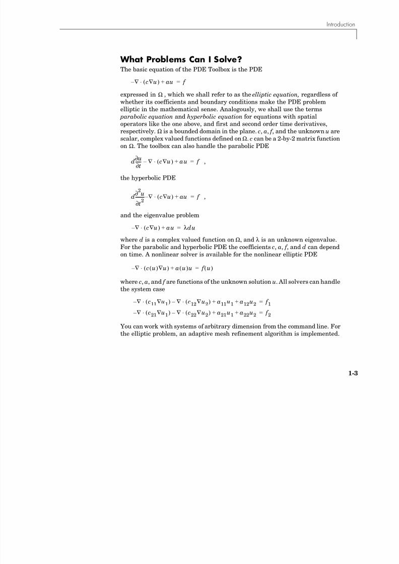
What Problems Can I Solve?The basic equation of the PDE Toolbox is the PDE
expressed in , which we shall refer to as the elliptic equation, regardless ofwhether its coefficients and boundary conditions make the PDE problemelliptic in the mathematical sense. Analogously, we shall use the terms parabolic equation and hyperbolic equation for equations with spatialoperators like the one above, and first and second order time derivatives,respectively. Ω is a bounded domain in the plane. c, a, f , and the unknown u arescalar, complex valued functions defined on Ω. c can be a 2-by-2 matrix functionon Ω. The toolbox can also handle the parabolic PDE
,
the hyperbolic PDE
,
and the eigenvalue problem
where d is a complex valued function on Ω, and λ is an unknown eigenvalue.For the parabolic and hyperbolic PDE the coefficients c, a, f , and d can dependon time. A nonlinear solver is available for the nonlinear elliptic PDE
where c, a, and f are functions of the unknown solution u. All solvers can handlethe system case
You can work with systems of arbitrary dimension from the command line. Forthe elliptic problem, an adaptive mesh refinement algorithm is implemented.
∇ – c u∇( )⋅ au+ f =
Ω
u∂t∂
------d ∇ – c u∇( )⋅ au+ f =
u2
∂
t∂2
---------d ∇ – c u∇( )⋅ au+ f =
∇ – c u∇( )⋅ au+ λdu=
∇ – c u( ) u∇( )⋅ a u( )u+ f u( )=
∇ – c11 u1∇( )⋅ ∇ – c12∇u2( )⋅ a11u1 a12u2+ + f 1=
∇ – c21 u1∇( )⋅ ∇ – c22∇u2( )⋅ a21u1 a22u2+ + f 2=
8/21/2019 matlab pde solving.pdf
http://slidepdf.com/reader/full/matlab-pde-solvingpdf 10/290
1 Tutorial
1-4
It can also be used in conjunction with the nonlinear solver. In addition, a fastsolver for Poisson’s equation on a rectangular grid is available.
The following boundary conditions are defined for scalar u:
• Dirichlet: hu = r on the boundary .
•Generalized Neumann: on .
is the outward unit normal. g, q, h, and r are complex-valued functions
defined on . (The eigenvalue problem is a homogeneous problem, i.e., g = 0,r = 0.) In the nonlinear case, the coefficients g, q, h, and r can depend on u, andfor the hyperbolic and parabolic PDE, the coefficients can depend on time. Forthe two-dimensional system case, Dirichlet boundary condition is
the generalized Neumann boundary condition is
and the mixed boundary condition is
,
where µ is computed such that the Dirichlet boundary condition is satisfied.Dirichlet boundary conditions are also called essential boundary conditions,and Neumann boundary conditions are also called natural boundary
conditions. See Chapter 4, “The Finite Element Method,” for the generalsystem case.
Ω∂
n c u∇( )⋅ qu+ g= Ω∂
n
Ω∂
h11u1 h12u2+ r1=
h21u1 h22u2+ r2=
n c21 u1∇( )⋅ n c22 u2∇( )⋅ q21u1 q22u2+ + + g2=
n c11 u1∇( )⋅ n c12 u2∇( )⋅ q11u1 q12u2+ + + g1=
h11u1 h12u2+ r1=
n c21 u1∇( )⋅ n c22 u2∇( )⋅ q21u1 q22u2+ + + g2 h12µ+=
n c11 u1∇( )⋅ n c12 u2∇( )⋅ q11u1 q12u2+ + + g1 h11µ+=
8/21/2019 matlab pde solving.pdf
http://slidepdf.com/reader/full/matlab-pde-solvingpdf 11/290
Introduction
1-5
In Which Areas Can the Toolbox Be Used?The PDEs implemented in the toolbox are used as a mathematical model for awide variety of phenomena in all branches of engineering and science. Thefollowing is by no means a complete list of examples.
The elliptic and parabolic equations are used for modeling
•Steady and unsteady heat transfer in solids
•
Flows in porous media and diffusion problems•Electrostatics of dielectric and conductive media
•Potential flow
The hyperbolic equation is used for
•Transient and harmonic wave propagation in acoustics and electromagnetics
•Transverse motions of membranes
The eigenvalue problems are used for
•Determining natural vibration states in membranes and structuralmechanics problems
Last, but not least, the toolbox can be used for educational purposes as acomplement to understanding the theory of the FEM.
How Do I Define a PDE Problem?The simplest way to define a PDE problem is using the GUI, implemented inpdetool. There are three modes that correspond to different stages of defininga PDE problem:
• In Draw mode, you create Ω, the geometry, using the constructive solidgeometry (CSG) model paradigm. A set of solid objects (rectangle, circle,ellipse, and polygon) is provided. You can combine these objects using set
formulas.• In Boundary mode, you specify the boundary conditions. You can have
different types of boundary conditions on different boundary segments.
8/21/2019 matlab pde solving.pdf
http://slidepdf.com/reader/full/matlab-pde-solvingpdf 12/290
1 Tutorial
1-6
•
In PDE mode , you interactively specify the type of PDE and the coefficientsc, a, f , and d. You can specify the coefficients for each subdomainindependently. This may ease the specification of, e.g., various materialproperties in a PDE model.
How Can I Solve a PDE Problem?Most problems can be solved from the GUI. There are two major modes that
help you solve a problem:• In Mesh mode, you generate and plot meshes. You can control the
parameters of the automated mesh generator.
• In Solve mode, you can invoke and control the nonlinear and adaptivesolvers for elliptic problems. For parabolic and hyperbolic problems, you canspecify the initial values, and the times for which the output should begenerated. For the eigenvalue solver, you can specify the interval in which to
search for eigenvalues. After solving a problem, you can return to the Mesh mode to further refine yourmesh and then solve again. You can also employ the adaptive mesh refiner andsolver. This option tries to find a mesh that fits the solution.
Can I Use the Toolbox for Nonstandard Problems?For advanced, nonstandard applications you can transfer the description of
domains, boundary conditions etc. to your MATLAB workspace. From thereyou use the functions of the PDE Toolbox for managing data on unstructuredmeshes. You have full access to the mesh generators, FEM discretizations ofthe PDE and boundary conditions, interpolation functions, etc. You can designyour own solvers or use FEM to solve subproblems of more complex algorithms.See also “Using Command-Line Functions” on page 1-40.
8/21/2019 matlab pde solving.pdf
http://slidepdf.com/reader/full/matlab-pde-solvingpdf 13/290
Introduction
1-7
How Can I Visualize My Results?From the graphical user interface you can use Plot mode, where you have awide range of visualization possibilities. You can visualize both inside thepdetool GUI and in separate figures. You can plot three different solutionproperties at the same time, using color, height, and vector field plots. Surface,mesh, contour, and arrow (quiver) plots are available. For surface plots, youcan choose between interpolated and flat rendering schemes. The mesh may behidden or exposed in all plot types. For parabolic and hyperbolic equations, you
can even produce an animated movie of the solution’s time dependence. All visualization functions are also accessible from the command line.
Are There Any Applications Already Implemented?The PDE Toolbox is easy to use in the most common areas due to theapplication interfaces. Eight application interfaces are available, in addition tothe generic scalar and system (vector valued u) cases:
• “Structural Mechanics — Plane Stress”• “Structural Mechanics — Plane Strain”
• “Electrostatics”
• “Magnetostatics”
• “AC Power Electromagnetics”
• “Conductive Media DC”
• “Heat Transfer” • “Diffusion”
These interfaces have dialog boxes where the PDE coefficients, boundaryconditions, and solution are explained in terms of physical entities. Theapplication interfaces enable you to enter specific parameters, such as Young’smodulus in the structural mechanics problems. Also, visualization of therelevant physical variables is provided.
Several nontrivial examples are included in this manual. Many examples aresolved both by using the GUI and in command-line mode.
The toolbox contains a number of demonstration M-files. They illustrate someways in which you can write your own applications.
8/21/2019 matlab pde solving.pdf
http://slidepdf.com/reader/full/matlab-pde-solvingpdf 14/290
1 Tutorial
1-8
Can I Extend the Functionality of the Toolbox?The PDE Toolbox is written using the MATLAB open system philosophy. Thereare no black-box functions, although some functions may not be easy tounderstand at first glance. The data structures and formats are documented. You can examine the existing functions and create your own as needed.
How Can I Solve 3-D Problems by 2-D Models?
The PDE Toolbox solves problems in two space dimensions and time, whereasreality has three space dimensions. The reduction to 2-D is possible when variations in the third space dimension (taken to be z) can be accounted for inthe 2-D equation. In some cases, like the plane stress analysis, the materialparameters must be modified in the process of dimensionality reduction.
When the problem is such that variation with z is negligible, all z-derivativesdrop out and the 2-D equation has exactly the same units and coefficients asin 3-D.
Slab geometries are treated by integration through the thickness. The result isa 2-D equation for the z-averaged solution with the thickness, say D( x, y),multiplied onto all the PDE coefficients, c, a, d, and f , etc. For instance, if youwant to compute the stresses in a sheet welded together from plates of differentthickness, multiply Young’s modulus E, volume forces, and specified surfacetractions by D( x, y). Similar definitions of the equation coefficients are called forin other slab geometry examples and application modes.

8/21/2019 matlab pde solving.pdf
http://slidepdf.com/reader/full/matlab-pde-solvingpdf 15/290
Getting Started
1-9
Getting StartedTo get you started, let us use the graphical user interface (GUI) pdetool, whichis a part of the PDE Toolbox, to solve a PDE step by step. The problem that wewould like to solve is Poisson’s equation, . The 2-D geometry on whichwe would like to solve the PDE is quite complex. The boundary conditions areof Dirichlet and Neumann types.
First, invoke MATLAB. To start the GUI, type the command pdetool at theMATLAB prompt. It can take a minute or two for the GUI to start. The GUIlooks similar to the figure below, with exception of the grid. Turn on the gridby selecting Grid from the Options menu. Also, enable the “snap-to-grid”feature by selecting Snap from the Options menu. The “snap-to-grid” featuresimplifies aligning the solid objects.
∆u – f =
8/21/2019 matlab pde solving.pdf
http://slidepdf.com/reader/full/matlab-pde-solvingpdf 16/290
1 Tutorial
1-10
The first step is to draw the geometry on which you want to solve the PDE. TheGUI provides four basic types of solid objects: polygons, rectangles, circles, andellipses. The objects are used to create a Constructive Solid Geometry model
(CSG model). Each solid object is assigned a unique label, and by the use of setalgebra, the resulting geometry can be made up of a combination of unions,intersections, and set differences. By default, the resulting CSG model is theunion of all solid objects.
To select a solid object, either click the button with an icon depicting the solid
object that you want to use, or select the object by using the Draw pull-downmenu. In this case, rectangle/square objects are selected. To draw a rectangleor a square starting at a corner, click the rectangle button without a + sign inthe middle. The button with the + sign is used when you want to draw startingat the center. Then, put the cursor at the desired corner, and click-and-dragusing the left mouse button to create a rectangle with the desired side lengths.(Use the right mouse button to create a square.) Notice how the “snap-to-grid”feature forces the rectangle to line up with the grid. When you release the
mouse, the CSG model is updated and redrawn. At this stage, all you have is arectangle. It is assigned the label R1. If you want to move or resize therectangle, you can easily do so. Click-and-drag an object to move it, anddouble-click an object to open a dialog box, where you can enter exact locationcoordinates. From the dialog box, you can also alter the label. If you are notsatisfied and want to restart, you can delete the rectangle by clicking theDelete key or by selecting Clear from the Edit menu. Next, draw a circle byclicking the button with the ellipse icon with the + sign, and then
click-and-drag in a similar way, using the right mouse button, starting at thecircle center.

8/21/2019 matlab pde solving.pdf
http://slidepdf.com/reader/full/matlab-pde-solvingpdf 17/290
Getting Started
1-11
The resulting CSG model is the union of the rectangle R1 and the circle C1,described by set algebra as R1+C1. The area where the two objects overlap isclearly visible as it is drawn using a darker shade of gray. The object that you just drew — the circle — has a black border, indicating that it is selected. Aselected object can be moved, resized, copied, and deleted. You can select morethan one object by Shift-clicking the objects that you want to select. Also, a
Select All option is available from the Edit menu.
8/21/2019 matlab pde solving.pdf
http://slidepdf.com/reader/full/matlab-pde-solvingpdf 18/290
1 Tutorial
1-12
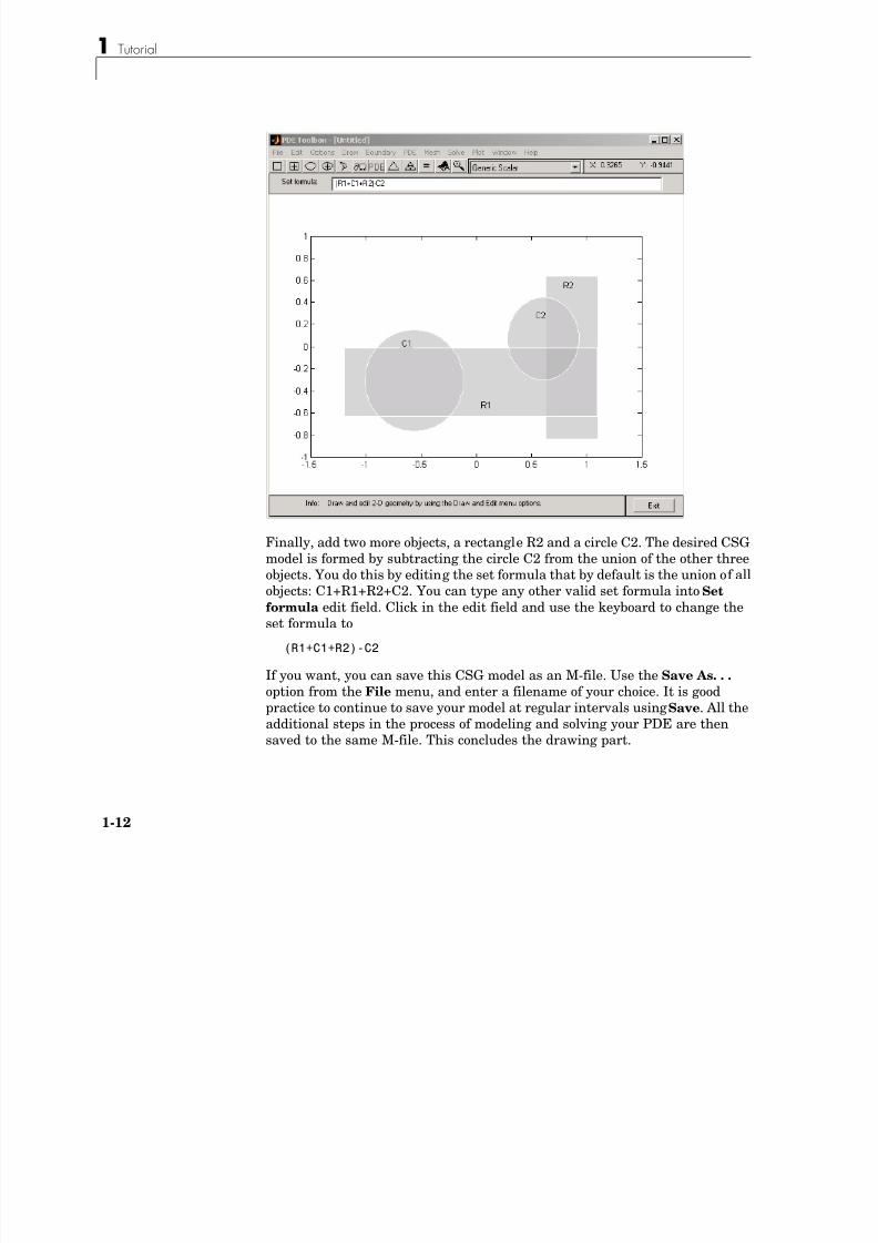
Finally, add two more objects, a rectangle R2 and a circle C2. The desired CSGmodel is formed by subtracting the circle C2 from the union of the other threeobjects. You do this by editing the set formula that by default is the union of allobjects: C1+R1+R2+C2. You can type any other valid set formula into Set
formula edit field. Click in the edit field and use the keyboard to change theset formula to
(R1+C1+R2)-C2
If you want, you can save this CSG model as an M-file. Use the Save As. . .
option from the File menu, and enter a filename of your choice. It is goodpractice to continue to save your model at regular intervals using Save. All theadditional steps in the process of modeling and solving your PDE are thensaved to the same M-file. This concludes the drawing part.

8/21/2019 matlab pde solving.pdf
http://slidepdf.com/reader/full/matlab-pde-solvingpdf 19/290
Getting Started
1-13
You can now define the boundary conditions for the outer boundaries. Enterthe Boundary Mode by clicking the icon or by selecting Boundary Mode from the Boundary menu. You can now remove subdomain borders and definethe boundary conditions.
The gray edge segments are subdomain borders induced by the intersections ofthe original solid objects. Borders that do not represent borders between, e.g.,areas with differing material properties, can be removed. From the Boundary menu, select the Remove All Subdomain Borders option. All borders are then
removed from the decomposed geometry.The boundaries are indicated by colored lines with arrows. The color reflectsthe type of boundary condition, and the arrow points toward the end of theboundary segment. The direction information is provided for the case when theboundary condition is parameterized along the boundary. The boundarycondition can also be a function of x and y, or simply a constant. By default, theboundary condition is of Dirichlet type: u = 0 on the boundary.
Dirichlet boundary conditions are indicated by red color. The boundaryconditions can also be of a generalized Neumann (blue) or mixed (green) type.For scalar u, however, all boundary conditions are either of Dirichlet or thegeneralized Neumann type. You select the boundary conditions that you wantto change by clicking to select one boundary segment, by Shift-clicking to selectmultiple segments, or by using the Edit menu option Select All to select allboundary segments. The selected boundary segments are indicated by blackcolor.
For this problem, change the boundary condition for all the circle arcs. Selectthem by using the mouse and Shift-click those boundary segments.
Ω∂
8/21/2019 matlab pde solving.pdf
http://slidepdf.com/reader/full/matlab-pde-solvingpdf 20/290
1 Tutorial
1-14
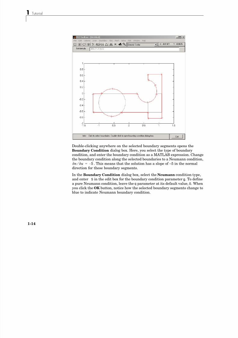
Double-clicking anywhere on the selected boundary segments opens theBoundary Condition dialog box. Here, you select the type of boundarycondition, and enter the boundary condition as a MATLAB expression. Changethe boundary condition along the selected boundaries to a Neumann condition,
. This means that the solution has a slope of –5 in the normaldirection for these boundary segments.
In the Boundary Condition dialog box, select the Neumann condition type,
and enter 5 in the edit box for the boundary condition parameter g. To definea pure Neumann condition, leave the q parameter at its default value, 0. Whenyou click the OK button, notice how the selected boundary segments change toblue to indicate Neumann boundary condition.
∂n ∂u ⁄ 5 – =
8/21/2019 matlab pde solving.pdf
http://slidepdf.com/reader/full/matlab-pde-solvingpdf 21/290
Getting Started
1-15
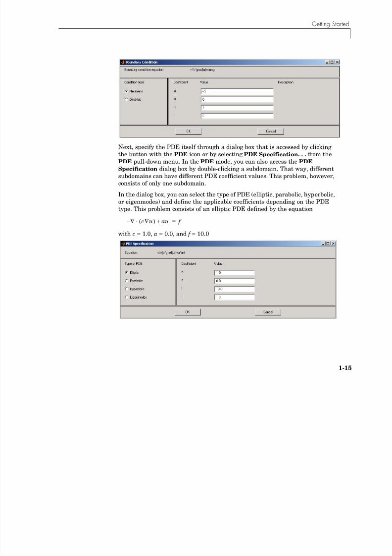
Next, specify the PDE itself through a dialog box that is accessed by clickingthe button with the PDE icon or by selecting PDE Specification. . . from thePDE pull-down menu. In the PDE mode, you can also access the PDE
Specification dialog box by double-clicking a subdomain. That way, different
subdomains can have different PDE coefficient values. This problem, however,consists of only one subdomain.
In the dialog box, you can select the type of PDE (elliptic, parabolic, hyperbolic,or eigenmodes) and define the applicable coefficients depending on the PDEtype. This problem consists of an elliptic PDE defined by the equation
with c = 1.0, a = 0.0, and f = 10.0
∇ – c∇u( )⋅ au+ f =
8/21/2019 matlab pde solving.pdf
http://slidepdf.com/reader/full/matlab-pde-solvingpdf 22/290
1 Tutorial
1-16
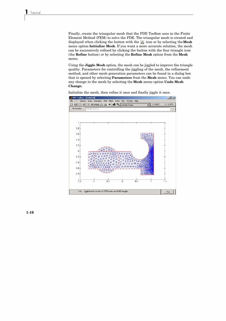
Finally, create the triangular mesh that the PDE Toolbox uses in the FiniteElement Method (FEM) to solve the PDE. The triangular mesh is created anddisplayed when clicking the button with the icon or by selecting the Mesh menu option Initialize Mesh. If you want a more accurate solution, the meshcan be successively refined by clicking the button with the four triangle icon(the Refine button) or by selecting the Refine Mesh option from the Mesh menu.
Using the Jiggle Mesh option, the mesh can be jiggled to improve the triangle
quality. Parameters for controlling the jiggling of the mesh, the refinementmethod, and other mesh generation parameters can be found in a dialog boxthat is opened by selecting Parameters from the Mesh menu. You can undoany change to the mesh by selecting the Mesh menu option Undo Mesh
Change.
Initialize the mesh, then refine it once and finally jiggle it once.
8/21/2019 matlab pde solving.pdf
http://slidepdf.com/reader/full/matlab-pde-solvingpdf 23/290
Getting Started
1-17
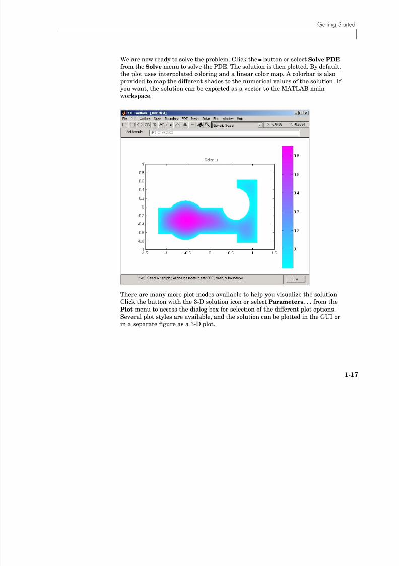
We are now ready to solve the problem. Click the = button or select Solve PDE from the Solve menu to solve the PDE. The solution is then plotted. By default,the plot uses interpolated coloring and a linear color map. A colorbar is alsoprovided to map the different shades to the numerical values of the solution. Ifyou want, the solution can be exported as a vector to the MATLAB mainworkspace.
There are many more plot modes available to help you visualize the solution.
Click the button with the 3-D solution icon or select Parameters. . . from thePlot menu to access the dialog box for selection of the different plot options.Several plot styles are available, and the solution can be plotted in the GUI orin a separate figure as a 3-D plot.
8/21/2019 matlab pde solving.pdf
http://slidepdf.com/reader/full/matlab-pde-solvingpdf 24/290
1 Tutorial
1-18
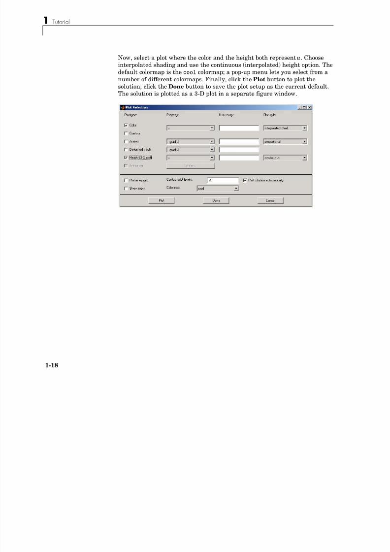
Now, select a plot where the color and the height both represent u. Chooseinterpolated shading and use the continuous (interpolated) height option. Thedefault colormap is the cool colormap; a pop-up menu lets you select from anumber of different colormaps. Finally, click the Plot button to plot thesolution; click the Done button to save the plot setup as the current default.The solution is plotted as a 3-D plot in a separate figure window.
8/21/2019 matlab pde solving.pdf
http://slidepdf.com/reader/full/matlab-pde-solvingpdf 25/290
Getting Started
1-19
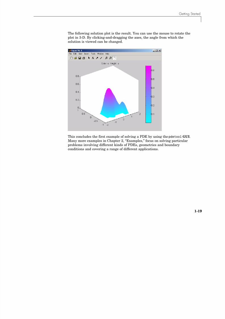
The following solution plot is the result. You can use the mouse to rotate theplot in 3-D. By clicking-and-dragging the axes, the angle from which thesolution is viewed can be changed.
This concludes the first example of solving a PDE by using the pdetool GUI.Many more examples in Chapter 2, “Examples,” focus on solving particularproblems involving different kinds of PDEs, geometries and boundaryconditions and covering a range of different applications.
8/21/2019 matlab pde solving.pdf
http://slidepdf.com/reader/full/matlab-pde-solvingpdf 26/290
1 Tutorial
1-20
Basics of the Finite Element MethodThe solutions of simple PDEs on complicated geometries can rarely beexpressed in terms of elementary functions. You are confronted with twoproblems: First you need to describe a complicated geometry and generate amesh on it. Then you need to discretize your PDE on the mesh and build anequation for the discrete approximation of the solution. The pdetool graphicaluser interface provides you with easy-to-use graphical tools to describe
complicated domains and generate triangular meshes. It also discretizes PDEs,finds discrete solutions and plots results. You can access the mesh structuresand the discretization functions directly from the command line (or M-file) andincorporate them into specialized applications.
Below is an overview of the Finite Element Method (FEM). The purpose of thispresentation is to get you acquainted with the elementary FEM notions. Hereyou find the precise equations that are solved and the nature of the discretesolution. Different extensions of the basic equation implemented in the PDE
Toolbox are presented. A more detailed description can be found in Chapter 4,“The Finite Element Method.”
You start by approximating the computational domain with a union ofsimple geometric objects, in this case triangles. The triangles form a mesh andeach vertex is called a node. You are in the situation of an architect designinga dome. He has to strike a balance between the ideal rounded forms of theoriginal sketch and the limitations of his simple building-blocks, triangles orquadrilaterals. If the result does not look close enough to a perfect dome, thearchitect can always improve his work using smaller blocks.
Next you say that your solution should be simple on each triangle. Polynomialsare a good choice: they are easy to evaluate and have good approximationproperties on small domains. You can ask that the solutions in neighboringtriangles connect to each other continuously across the edges. You can stilldecide how complicated the polynomials can be. Just like an architect, youwant them as simple as possible. Constants are the simplest choice but you
cannot match values on neighboring triangles. Linear functions come next.
Ω
8/21/2019 matlab pde solving.pdf
http://slidepdf.com/reader/full/matlab-pde-solvingpdf 27/290
Basics of the Finite Element Method
1-21
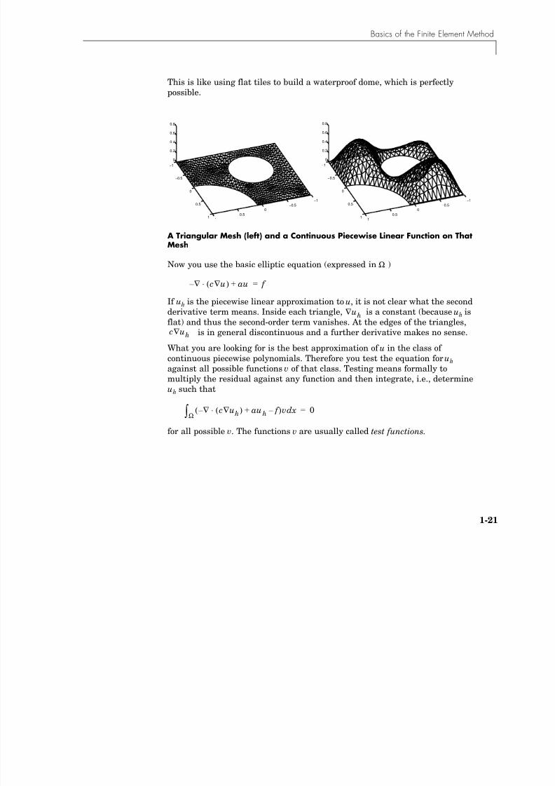
This is like using flat tiles to build a waterproof dome, which is perfectlypossible.
A Triangular Mesh (left) and a Continuous Piecewise Linear Function on ThatMesh
Now you use the basic elliptic equation (expressed in )
If uh is the piecewise linear approximation to u, it is not clear what the secondderivative term means. Inside each triangle, is a constant (because uh isflat) and thus the second-order term vanishes. At the edges of the triangles,
is in general discontinuous and a further derivative makes no sense.What you are looking for is the best approximation of u in the class ofcontinuous piecewise polynomials. Therefore you test the equation for uh against all possible functions v of that class. Testing means formally tomultiply the residual against any function and then integrate, i.e., determineuh such that
for all possible v. The functions v are usually called test functions.
−1
−0.5
0
0.5
1
−1
−0.5
0
0.5
1
0
0.2
0.4
0.6
0.8
−1
−0.5
0
0.5
1
−1
−0.5
0
0.5
1
0
0.2
0.4
0.6
0.8
Ω
∇ – c u∇( )⋅ au+ f =
uh∇
c uh∇
∇ – c uh∇( )⋅ auh f – +( )v xdΩ! 0=
8/21/2019 matlab pde solving.pdf
http://slidepdf.com/reader/full/matlab-pde-solvingpdf 28/290
1 Tutorial
1-22
Partial integration (Green’s formula) yields that uh should satisfy
where is the boundary of and is the outward pointing normal on .Note that the integrals of this formulation are well-defined even if uh and v arepiecewise linear functions.
Boundary conditions are included in the following way. If uh is known at some
boundary points (Dirichlet boundary conditions), we restrict the test functionsto v = 0 at those points, and require uh to attain the desired value at that point. At all the other points we ask for Neumann boundary conditions, i.e.,
. The FEM formulation reads: Find uh such that
where is the part of the boundary with Neumann conditions. The testfunctions v must be zero on .
Any continuous piecewise linear uh is represented as a combination
where φi are some special piecewise linear basis functions and U i are scalarcoefficients. Choose φi like a tent, such that it has the “height” 1 at the node i
and the height 0 at all other nodes. For any fixed v, the FEM formulation yieldsan algebraic equation in the unknowns U i. You want to determine N unknowns, so you need N different instances of v. What better candidates thanv = φ j, j = 1, 2, . . . , N ? You find a linear system KU = F where the matrix K andthe right side F contain integrals in terms of the test functions φi, φ j and thecoefficients defining the problem: c, a, f, q, and g. The solution vector U containsthe expansion coefficients of uh, which are also the values of uh at each node xi since uh(xi ) = U i.
If the exact solution u is smooth, then FEM computes uh with an error of thesame size as that of the linear interpolation. It is possible to estimate the erroron each triangle using only uh and the PDE coefficients (but not the exactsolution u, which in general is unknown).
c uh∇( ) v∇Ω! auhvdx n
∂Ω! – + c uh∇( )vds⋅ fv xdΩ!= v∀
Ω∂ Ω n Ω∂
c∇uh( ) n⋅ quh+ g=
c uh∇( ) v∇Ω! auhvdx quhvds
∂Ω 1!+ + fv xdΩ!= gv sd
∂Ω 1!+ v∀
∂Ω1 ∂Ω ∂Ω1 –
uh x( ) U iφi x( )i 1=
N
"=
8/21/2019 matlab pde solving.pdf
http://slidepdf.com/reader/full/matlab-pde-solvingpdf 29/290
Basics of the Finite Element Method
1-23
The PDE Toolbox provides functions that assemble K and F . This is doneautomatically in the graphical user interface, but you also have direct access tothe FEM matrices from the command-line function assempde.
To summarize, the FEM approach is to approximate the PDE solution u by apiecewise linear function is expanded in a basis of test-functions φi,and the residual is tested against all the basis functions. This procedure yieldsa linear system KU = F. The components of U are the values of uh at the nodes.For x inside a triangle, uh(x) is found by linear interpolation from the nodal
values.FEM techniques are also used to solve more general problems. Below are somegeneralizations that you can access both through the graphical user interfaceand with command-line functions.
•Time-dependent problems are easy to implement in the FEM context. Thesolution u(x,t) of the equation
can be approximated by
•This yields a system of ordinary differential equations (ODE)
which you integrate using ODE solvers. Two time derivatives yield a secondorder ODE
etc. The toolbox supports problems with one or two time derivatives (thefunctions parabolic and hyperbolic).
uh uh⋅
u∂ t∂------d ∇ – c u∇( )⋅ au+ f =
uh x t,( ) U i t( )φ i x( )i 1=
N
"=
M td d U KU + F =
M t2
2
d
d U KU + F =
8/21/2019 matlab pde solving.pdf
http://slidepdf.com/reader/full/matlab-pde-solvingpdf 30/290
1 Tutorial
1-24
•
Eigenvalue problems: Solve
for the unknowns u and λ (λ is a complex number). Using the FEMdiscretization, you solve the algebraic eigenvalue problem KU = λh MU to finduh and λh as approximations to u and λ. A robust eigenvalue solver isimplemented in pdeeig.
• If the coefficients c, a, f, q, or g are functions of u, the PDE is called nonlinear
and FEM yields a nonlinear system K(U) U= F(U). You can use iterativemethods for solving the nonlinear system. The toolbox provides a nonlinearsolver called pdenonlin using a damped Gauss-Newton method.
•Small triangles are needed only in those parts of the computational domainwhere the error is large. In many cases the errors are large in a small regionand making all triangles small is a waste of computational effort. Makingsmall triangles only where needed is called adapting the mesh refinement tothe solution. An iterative adaptive strategy is the following: For a givenmesh, form and solve the linear system KU = F . Then estimate the error andrefine the triangles in which the error is large. The iteration is controlled byadaptmesh and the error is estimated by pdejmps.
Although the basic equation is scalar, systems of equations are also handled bythe toolbox. The interactive environment accepts u as a scalar or 2-vectorfunction. In command-line mode, systems of arbitrary size are accepted.
If c ≥ δ > 0 and a ≥ 0, under rather general assumptions on the domain Ω andthe boundary conditions, the solution u exists and is unique. The FEM linearsystem has a unique solution which converges to u as the triangles becomesmaller. The matrix K and the right side F make sense even when u does notexist or is not unique. It is advisable that you devise checks to problems withquestionable solutions.
∇ – c∇u( )⋅ au+ λdu=
8/21/2019 matlab pde solving.pdf
http://slidepdf.com/reader/full/matlab-pde-solvingpdf 31/290
Using the PDE Toolbox Graphical User Interface
1-25
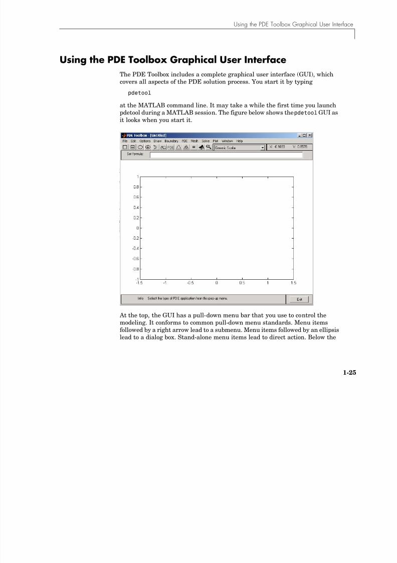
Using the PDE Toolbox Graphical User InterfaceThe PDE Toolbox includes a complete graphical user interface (GUI), whichcovers all aspects of the PDE solution process. You start it by typing
pdetool
at the MATLAB command line. It may take a while the first time you launchpdetool during a MATLAB session. The figure below shows the pdetool GUI as
it looks when you start it.
At the top, the GUI has a pull-down menu bar that you use to control themodeling. It conforms to common pull-down menu standards. Menu itemsfollowed by a right arrow lead to a submenu. Menu items followed by an ellipsislead to a dialog box. Stand-alone menu items lead to direct action. Below the
8/21/2019 matlab pde solving.pdf
http://slidepdf.com/reader/full/matlab-pde-solvingpdf 32/290
1 Tutorial
1-26
menu bar, a toolbar with icon buttons provide quick and easy access to some ofthe most important functions.
To the right of the toolbar is a pop-up menu that indicates the currentapplication mode. You can also use it to change the application mode. Theupper right part of the GUI also provides the x- and y-coordinates of the currentcursor position. It is updated when you move the cursor inside the main axesarea in the middle of the GUI. The edit box for the set formula contains theactive set formula. In the main axes you draw the 2-D geometry, display the
mesh, plot the solution, etc. At the bottom of the GUI, an information lineprovides information about the current activity. It can also display helpinformation about the toolbar buttons.
The MenusThere are 11 different pull-down menus in the GUI. See Chapter 3, “TheGraphical User Interface,” for a more detailed description of the menus and the
dialog boxes:•File menu. From the File menu you can Open and Save model M-files that
contain a command sequence that reproduces your modeling session. Youcan also print the current graphics and exit the GUI.
•Edit menu. From the Edit menu you can cut, clear, copy, and paste the solidobjects. There is also a Select All option.
•Options menu. The Options menu contains options such as toggling the axis
grid, a “snap-to-grid” feature, and zoom. You can also adjust the axis limitsand the grid spacing, select the application mode, and refresh the GUI.
•Draw menu. From the Draw menu you can select the basic solid objects suchas circles and polygons. You can then draw objects of the selected type usingthe mouse. From the Draw menu you can also rotate the solid objects andexport the geometry to the MATLAB main workspace.
•Boundary menu. From the Boundary menu you access a dialog box whereyou define the boundary conditions. Additionally, you can label edges andsubdomains, remove borders between subdomains, and export thedecomposed geometry and the boundary conditions to the workspace.
•PDE menu. The PDE menu provides a dialog box for specifying the PDE, andthere are menu options for labeling subdomains and exporting PDEcoefficients to the workspace.
8/21/2019 matlab pde solving.pdf
http://slidepdf.com/reader/full/matlab-pde-solvingpdf 33/290
Using the PDE Toolbox Graphical User Interface
1-27
•
Mesh menu. From the Mesh menu you create and modify the triangularmesh. You can initialize, refine, and jiggle the mesh, undo previous meshchanges, label nodes and triangles, display the mesh quality, and export themesh to the workspace.
•Solve menu. From the Solve menu you solve the PDE. You can also open adialog box where you can adjust the solve parameters, and you can export thesolution to the workspace.
•Plot menu. From the Plot menu you can plot a solution property. A dialog
box lets you select which property to plot, which plot style to use and severalother plot parameters. If you have recorded a movie (animation) of thesolution, you can export it to the workspace.
•Window menu. The Window menu lets you select any currently openMATLAB figure window. The selected window is brought to the front.
•Help menu. The Help menu provides a brief help window.
The ToolbarThe toolbar underneath the main menu at the top of the GUI contains iconbuttons that provide quick and easy access to some of the most importantfunctions.
The five leftmost buttons are Draw mode buttons and they represent, from leftto right:
Draw a rectangle/square starting at a corner.
Draw a rectangle/square starting at the center.
Draw an ellipse/circle starting at the perimeter.
Draw an ellipse/circle starting at the center.
Draw a polygon. Click-and-drag to create polygon sides. You canclose the polygon by clicking the right mouse button. Clicking atthe starting vertex also closes the polygon.
8/21/2019 matlab pde solving.pdf
http://slidepdf.com/reader/full/matlab-pde-solvingpdf 34/290
1 Tutorial
1-28
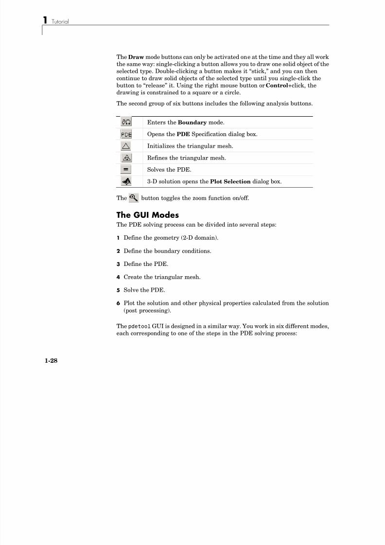
The Draw mode buttons can only be activated one at the time and they all workthe same way: single-clicking a button allows you to draw one solid object of theselected type. Double-clicking a button makes it “stick,” and you can thencontinue to draw solid objects of the selected type until you single-click thebutton to “release” it. Using the right mouse button or Control+click, thedrawing is constrained to a square or a circle.
The second group of six buttons includes the following analysis buttons.
The button toggles the zoom function on/off.
The GUI ModesThe PDE solving process can be divided into several steps:
1 Define the geometry (2-D domain).
2 Define the boundary conditions.
3 Define the PDE.
4 Create the triangular mesh.
5 Solve the PDE.6 Plot the solution and other physical properties calculated from the solution
(post processing).
The pdetool GUI is designed in a similar way. You work in six different modes,each corresponding to one of the steps in the PDE solving process:
Enters the Boundary mode.
Opens the PDE Specification dialog box.
Initializes the triangular mesh.
Refines the triangular mesh.
Solves the PDE.
3-D solution opens the Plot Selection dialog box.
8/21/2019 matlab pde solving.pdf
http://slidepdf.com/reader/full/matlab-pde-solvingpdf 35/290
Using the PDE Toolbox Graphical User Interface
1-29
•
InDraw mode
, you can create the 2-D geometry using the constructive solidgeometry (CSG) model paradigm. A set of solid objects (rectangle, circle,ellipse, and polygon) is provided. These objects can be combined using setformulas in a flexible way.
• In Boundary mode, you can specify the boundary conditions. You can havedifferent types of boundary conditions on different boundaries. In this mode,the original shapes of the solid objects constitute borders betweensubdomains of the model. Such borders can be eliminated in this mode.
• In PDE mode , you can interactively specify the type of PDE problem, and thePDE coefficients. You can specify the coefficients for each subdomainindependently. This makes it easy to specify, e.g., various materialproperties in a PDE model.
• In Mesh mode , you can control the automated mesh generation and plot themesh.
• In Solve mode , you can invoke and control the nonlinear and adaptive solver
for elliptic problems. For parabolic and hyperbolic PDE problems, you canspecify the initial values, and the times for which the output should begenerated. For the eigenvalue solver, you can specify the interval in which tosearch for eigenvalues.
• In Plot mode there is wide range of visualization possibilities. You can visualize both in the pdetool GUI and in a separate figure window. You can visualize three different solution properties at the same time, using color,height, and vector field plots. There are surface, mesh, contour, and arrow(quiver) plots available. For parabolic and hyperbolic equations, you cananimate the solution as it changes with time.
8/21/2019 matlab pde solving.pdf
http://slidepdf.com/reader/full/matlab-pde-solvingpdf 36/290
1 Tutorial
1-30
The CSG Model and the Set FormulaThe PDE Toolbox uses the Constructive Solid Geometry (CSG) model paradigmfor the modeling. You can draw solid objects that can overlap. There are fourtypes of solid objects:
•Circle object — Represents the set of points inside and on a circle.
•Polygon object — Represents the set of points inside and on a polygon givenby a set of line segments.
•Rectangle object — Represents the set of points inside and on a rectangle.•Ellipse object — Represents the set of points inside and on an ellipse. The
ellipse can be rotated.
Each solid object is automatically given a unique name by the GUI. The defaultnames are C1, C2, C3, etc., for circles; P1, P2, P3, etc. for polygons; R1, R2, R3,etc., for rectangles; E1, E2, E3, etc., for ellipses. Squares, although a specialcase of rectangles, are named SQ1, SQ2, SQ3, etc. The name is displayed on the
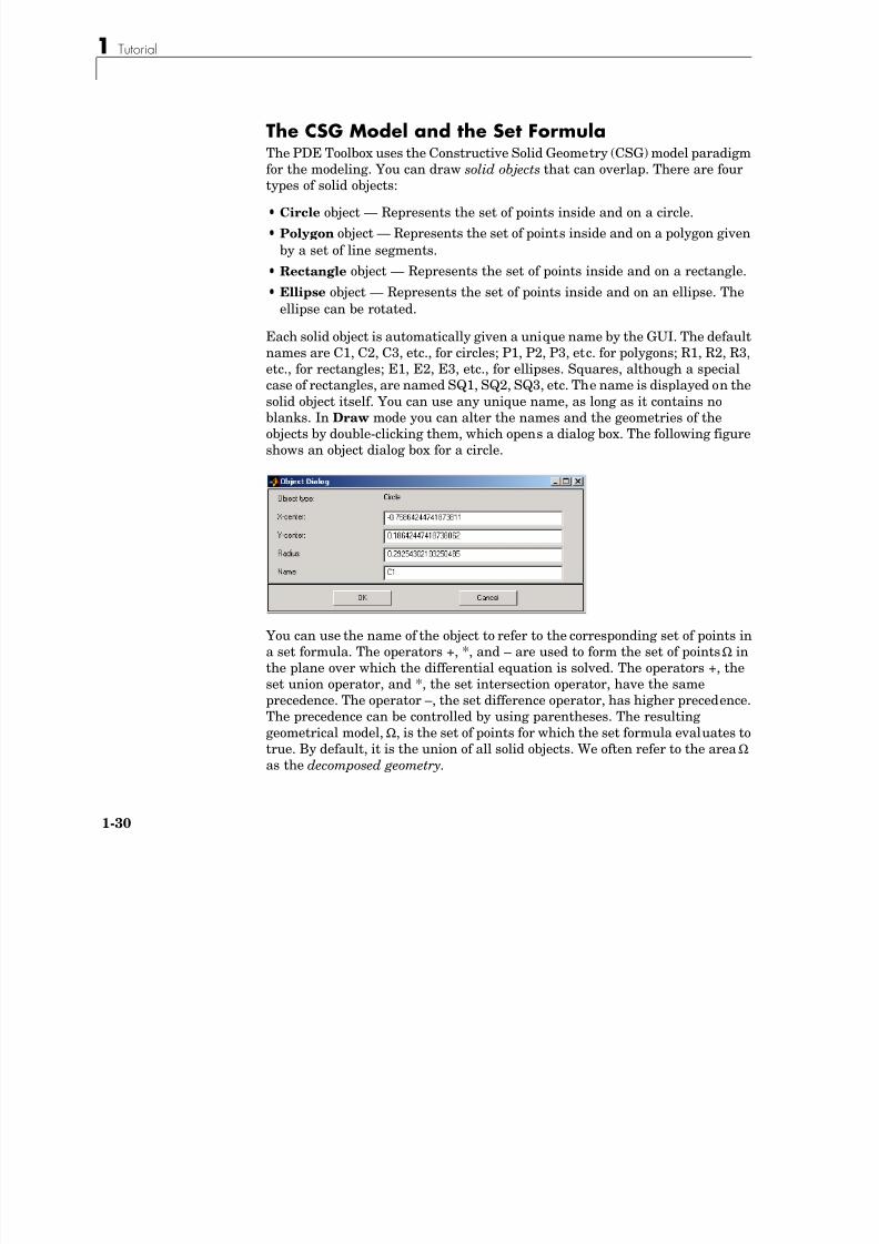
solid object itself. You can use any unique name, as long as it contains noblanks. In Draw mode you can alter the names and the geometries of theobjects by double-clicking them, which opens a dialog box. The following figureshows an object dialog box for a circle.
You can use the name of the object to refer to the corresponding set of points ina set formula. The operators +, *, and – are used to form the set of points Ω in
the plane over which the differential equation is solved. The operators +, theset union operator, and *, the set intersection operator, have the sameprecedence. The operator –, the set difference operator, has higher precedence.The precedence can be controlled by using parentheses. The resultinggeometrical model, Ω, is the set of points for which the set formula evaluates totrue. By default, it is the union of all solid objects. We often refer to the area Ω as the decomposed geometry.
8/21/2019 matlab pde solving.pdf
http://slidepdf.com/reader/full/matlab-pde-solvingpdf 37/290
Using the PDE Toolbox Graphical User Interface
1-31
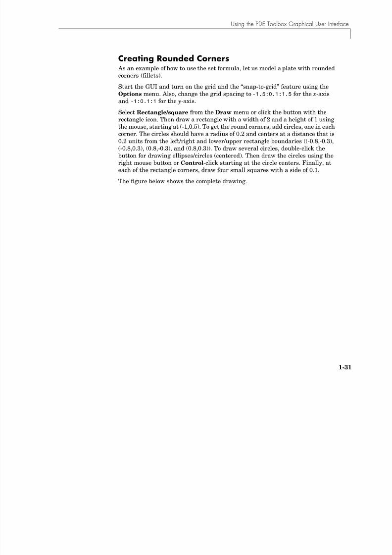
Creating Rounded Corners As an example of how to use the set formula, let us model a plate with roundedcorners (fillets).
Start the GUI and turn on the grid and the “snap-to-grid” feature using theOptions menu. Also, change the grid spacing to -1.5:0.1:1.5 for the x-axisand -1:0.1:1 for the y-axis.
Select Rectangle/square from the Draw menu or click the button with the
rectangle icon. Then draw a rectangle with a width of 2 and a height of 1 usingthe mouse, starting at (-1,0.5). To get the round corners, add circles, one in eachcorner. The circles should have a radius of 0.2 and centers at a distance that is0.2 units from the left/right and lower/upper rectangle boundaries ((-0.8,-0.3),(-0.8,0.3), (0.8,-0.3), and (0.8,0.3)). To draw several circles, double-click thebutton for drawing ellipses/circles (centered). Then draw the circles using theright mouse button or Control-click starting at the circle centers. Finally, ateach of the rectangle corners, draw four small squares with a side of 0.1.
The figure below shows the complete drawing.
1
8/21/2019 matlab pde solving.pdf
http://slidepdf.com/reader/full/matlab-pde-solvingpdf 38/290
1 Tutorial
1-32
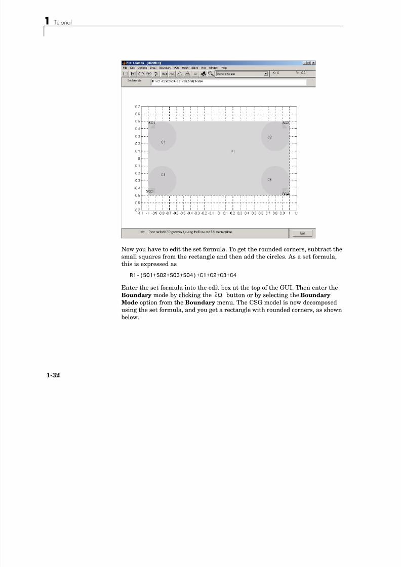
Now you have to edit the set formula. To get the rounded corners, subtract thesmall squares from the rectangle and then add the circles. As a set formula,this is expressed as
R1-(SQ1+SQ2+SQ3+SQ4)+C1+C2+C3+C4
Enter the set formula into the edit box at the top of the GUI. Then enter theBoundary mode by clicking the button or by selecting the Boundary
Mode option from the Boundary menu. The CSG model is now decomposedusing the set formula, and you get a rectangle with rounded corners, as shownbelow.
Ω∂
8/21/2019 matlab pde solving.pdf
http://slidepdf.com/reader/full/matlab-pde-solvingpdf 39/290
Using the PDE Toolbox Graphical User Interface
1-33
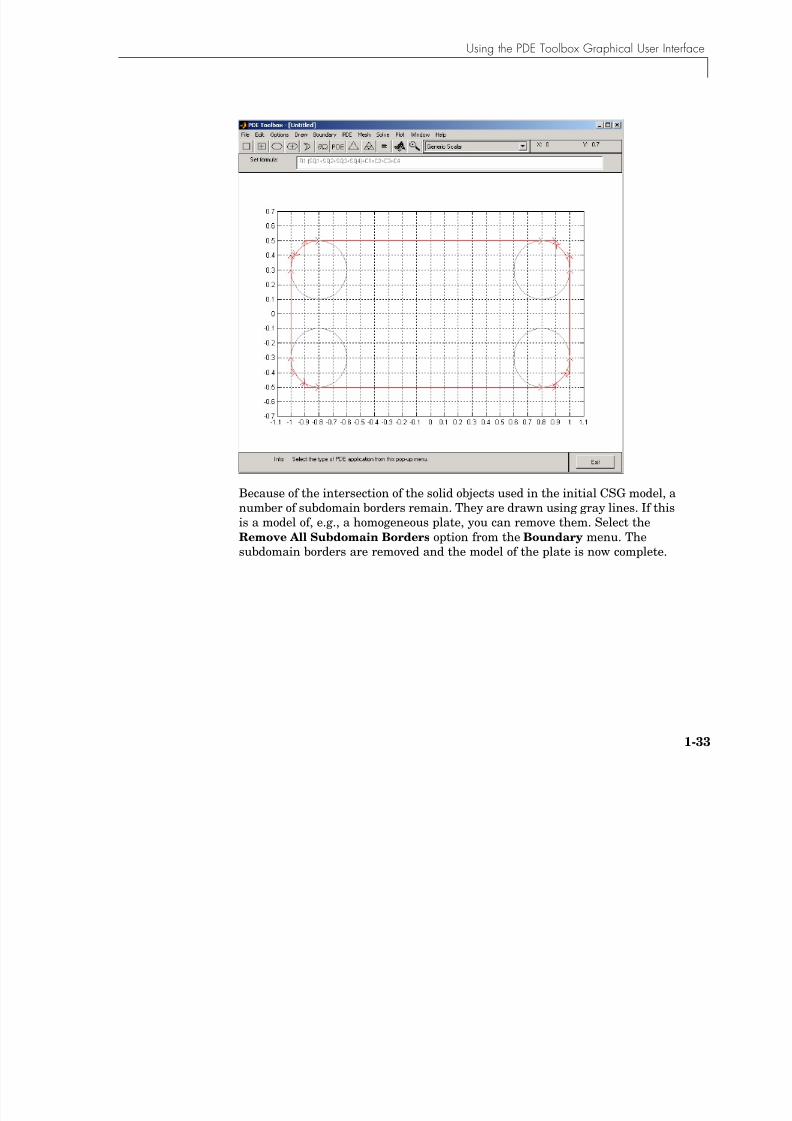
Because of the intersection of the solid objects used in the initial CSG model, anumber of subdomain borders remain. They are drawn using gray lines. If thisis a model of, e.g., a homogeneous plate, you can remove them. Select theRemove All Subdomain Borders option from the Boundary menu. Thesubdomain borders are removed and the model of the plate is now complete.
1
8/21/2019 matlab pde solving.pdf
http://slidepdf.com/reader/full/matlab-pde-solvingpdf 40/290
1 Tutorial
1-34
Suggested Modeling Method Although the PDE Toolbox offers you a great deal of flexibility in the ways thatyou can approach the problems and interact with the toolbox functions, thereis a suggested method of choice for modeling and solving your PDE problemsusing the pdetool GUI. There are also a number of shortcuts that you can usein certain situations.
Note There are platform-dependent keyboard accelerators available formany of the most common pdetool GUI activities. Learning to use theaccelerator keys may improve the efficiency of your pdetool sessions.
The basic flow of actions is indicated by the way the graphical buttons and themenus are ordered from left to right. You work your way from left to right inthe process of modeling, defining, and solving your PDE problem using the
pdetool GUI:•When you start, pdetool is in a Draw mode, where you can use the four basic
solid objects to draw your Constructive Solid Geometry (CSG) model. Youcan also edit the set formula. The solid objects are selected using the fiveleftmost buttons (or from the Draw menu).
•To the right of the Draw mode buttons you find buttons through which youcan access all the functions that you need to define and solve the PDEproblem: define boundary conditions, design the triangular mesh, solve thePDE, and plot the solution.
The following sequence of actions covers all the steps of a normal pdetool session:
1 Use pdetool as a drawing tool to make a drawing of the 2-D geometry onwhich you want to solve your PDE. Make use of the four basic solid objectsand the grid and the “snap-to-grid” feature. The GUI starts in the Draw
mode, and you can select the type of object that you want to use by clickingthe corresponding button or by using the Draw pull-down menu. Combinethe solid objects and the set algebra to build the desired CSG model.
8/21/2019 matlab pde solving.pdf
http://slidepdf.com/reader/full/matlab-pde-solvingpdf 41/290
Using the PDE Toolbox Graphical User Interface
1-35
2 Save the geometry to a model file. The model file is an M-file, so if you wantto continue working using the same geometry at your next PDE Toolboxsession, simply type the name of the model file at the MATLAB prompt. Thepdetool GUI then starts with the model file’s solid geometry loaded. If yousave the PDE problem at a later stage of the solution process, the model filealso contains commands to recreate the boundary conditions, the PDEcoefficients, and the mesh.
3 Move to the next step in the PDE solving process by clicking the button.
The outer boundaries of the decomposed geometry are displayed with thedefault boundary condition indicated. If the outer boundaries do not matchthe geometry of your problem, reenter the Draw mode. You can then correctyour CSG model by adding, removing or altering any of the solid objects, orchange the set formula used to evaluate the CSG model.
Note The set formula can only be edited while you are in the Draw mode.
If the drawing process resulted in any unwanted subdomain borders, removethem by using the Remove Subdomain Border or Remove All Subdomain
Borders option from the Boundary menu.
You can now define your problem’s boundary conditions by selecting theboundary to change and open a dialog box by double-clicking the boundary
or by using the Specify Boundary Conditions. . . option from the Boundary menu.
4 Initialize the triangular mesh. Click the ∆ button or use the correspondingMesh menu option Initialize Mesh. Normally, the mesh algorithm’s defaultparameters generate a good mesh. If necessary, they can be accessed usingthe Parameters. . . menu item.
5 If you need a finer mesh, the mesh can be refined by clicking the Refinebutton. Clicking the button several times causes a successive refinement ofthe mesh. The cost of a very fine mesh is a significant increase in the numberof points where the PDE is solved and, consequently, a significant increasein the time required to compute the solution. Do not refine unless it isrequired to achieve the desired accuracy. For each refinement, the numberof triangles increases by a factor of four. A better way to increase the
Ω∂
1
8/21/2019 matlab pde solving.pdf
http://slidepdf.com/reader/full/matlab-pde-solvingpdf 42/290
1 Tutorial
1-36
accuracy of the solution to elliptic PDE problems is to use the adaptivesolver, which refines the mesh in the areas where the estimated error of thesolution is largest. See the reference page for adaptmesh on page 5-9 for anexample of how the adaptive solver can solve a Laplace equation with anaccuracy that requires more than 10 times as many triangles when regularrefinement is used.
6 Specify the PDE from the PDE Specification dialog box. You can accessthat dialog box using the PDE button or the PDE Specification. . . menu
item from the PDE menu.
Note This step can be performed at any time prior to solving the PDE since itis independent of the CSG model and the boundaries. If the PDE coefficientsare material dependent, they are entered in the PDE mode by double-clickingthe different subdomains.
7 Solve the PDE by clicking the = button or by selecting Solve PDE from theSolve menu. If you do not want an automatic plot of the solution, or if youwant to change the way the solution is presented, you can do that from thePlot Selection dialog box prior to solving the PDE. You open the Plot
Selection dialog box by clicking the button with the 3-D solution plot icon orby selecting the Parameters. . . menu item from the Plot menu.
8 Now, from here you can choose one of several alternatives:•Export the solution and/or the mesh to the MATLAB main workspace for
further analysis.
• Visualize other properties of the solution.
•Change the PDE and recompute the solution.
•Change the mesh and recompute the solution. If you select Initialize
Mesh, the mesh is initialized; if you select Refine Mesh, the current mesh
is refined. From the Mesh menu, you can also jiggle the mesh and undoprevious mesh changes.
•Change the boundary conditions. To return to the mode where you can se-lect boundaries, use the button or the Boundary Mode option fromthe Boundary menu.
Ω∂
8/21/2019 matlab pde solving.pdf
http://slidepdf.com/reader/full/matlab-pde-solvingpdf 43/290
Using the PDE Toolbox Graphical User Interface
1-37
• Change the CSG model. You can reenter the draw mode by selecting Draw
Mode from the Draw menu or by clicking one of the Draw mode icons toadd another solid object. Back in the Draw mode, you are able to add,change, or delete solid objects and also to alter the set formula.
In addition to the recommended path of actions, there are a number ofshortcuts, which allow you to skip over one or more steps. In general, thepdetool GUI adds the necessary steps automatically.
• If you have not yet defined a CSG model, and leave the Draw mode with anempty model, pdetool creates an L-shaped geometry with the defaultboundary condition and then proceeds to the action called for, performing allthe steps necessary.
• If you are in the Draw mode and click the ∆ button to initialize the mesh,pdetool first decomposes the geometry using the current set formula andassigns the default boundary condition to the outer boundaries. After that,
an initial mesh is created.• If you click the refine button to refine the mesh before the mesh has been
initialized, pdetool first initializes the mesh (and decomposes the geometry,if you were still in the Draw mode).
• If you click the = button to solve the PDE and you have not yet created amesh, pdetool initializes a mesh before solving the PDE.
• If you select a plot type and choose to plot the solution, pdetool checks to seeif there is a solution to the current PDE available. If not, pdetool first solvesthe current PDE. The solution is then displayed using the selected plotoptions.
• If you have not defined your PDE, pdetool solves the default PDE, which isPoisson’s equation:
(This corresponds to the generic elliptic PDE with c = 1, a = 0, and f = 10.)
For the different application modes, different default PDE settings apply.
∆u – 10=
1 T l
8/21/2019 matlab pde solving.pdf
http://slidepdf.com/reader/full/matlab-pde-solvingpdf 44/290
1 Tutorial
1-38
Object Selection MethodsThroughout the GUI, similar principles apply for selecting objects such as solidobjects, subdomains, and boundaries.
•To select a single object, click it using the left mouse button.
•To select several objects and to deselect objects, Shift-click (or click usingthe middle mouse button) on the desired objects.
•Clicking in the intersection of several objects selects all the intersecting
objects.•To open an associated dialog box, double-click an object. If the object is
not selected, it is selected before opening the dialog box.
• In Draw mode and PDE mode, clicking outside of objects deselects allobjects.
•To select all objects, use the Select All option from the Edit menu.
•When defining boundary conditions and the PDE via the menu items from
the Boundary and PDE menus, and no boundaries or subdomains areselected, the entered values applies to all boundaries and subdomains bydefault.
Display Additional InformationIn Mesh mode, you can use the mouse to display the node number and thetriangle number at the position where you click. Press the left mouse button to
display the node number on the information line. Press the middle mousebutton (or use the left mouse button and the Shift key) to display the trianglenumber on the information line.
In Plot mode, you can use the mouse to display the numerical value of theplotted property at the position where you click. Press the left mouse button todisplay the triangle number and the value of the plotted property on theinformation line.
The information remains on the information line until you release the mousebutton.
8/21/2019 matlab pde solving.pdf
http://slidepdf.com/reader/full/matlab-pde-solvingpdf 45/290
Using the PDE Toolbox Graphical User Interface
1-39
Entering Parameter Values as MATLAB ExpressionsWhen entering parameter values, e.g., as a function of x and y, the enteredstring must be a MATLAB expression to be evaluated for x and y defined on thecurrent mesh, i.e., x and y are MATLAB row vectors. For example, the function4 x y should be entered as 4*x.*y and not as 4*x*y, which normally is not a valid MATLAB expression.
Using Earlier Version PDE Toolbox Model M-Files You can convert Model M-files created using an earlier version of the PDEToolbox for use with the current versions of MATLAB and the PDE Toolbox.The old Model M-files cannot be used directly in the current version of the PDEToolbox.
To convert your old Model M-files, use the conversion utility pdemdlcv. Forexample, to convert a Model M-file called model42.m to a compatible ModelM-file called model5.m, type the following at the MATLAB command line:
pdemdlcv model42 model5
1 T t i l
8/21/2019 matlab pde solving.pdf
http://slidepdf.com/reader/full/matlab-pde-solvingpdf 46/290
1 Tutorial
1-40
Using Command-Line Functions Although the pdetool GUI provides a convenient working environment, thereare situations where the flexibility of using the command-line functions isneeded. These include
•Geometrical shapes other than straight lines, circular arcs, and ellipticalarcs
•Nonstandard boundary conditions
•Complicated PDE or boundary condition coefficients
•More than two dependent variables in the system case
•Nonlocal solution constraints
•Special solution data processing and presentation itemize
The GUI can still be a valuable aid in some of the situations presented above,if part of the modeling is done using the GUI and then made available for
command-line use through the extensive data export facilities of the GUI.
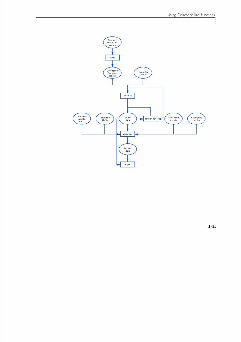
Data Structures and Utility FunctionsThe process of defining your problem and solving it is reflected in the design ofthe GUI. A number of data structures define different aspects of the problem,and the various processing stages produce new data structures out of old ones.See the figure following.
The rectangles are functions, and ellipses are data represented by matrices orM-files. Arrows indicate data necessary for the functions.
As there is a definite direction in this diagram, you can cut into it by presentingthe needed data sets, and then continue downward. In the sections below wegive pointers to descriptions of the precise formats of the various datastructures and M-files.
U C d L F
8/21/2019 matlab pde solving.pdf
http://slidepdf.com/reader/full/matlab-pde-solvingpdf 47/290
Using Command-Line Functions
1-41
Geometry
Description
matr i x
Decomposed
Geometry
matr ix
Mesh
data
Geometry
M-fi le
Coefficient
matr i x
Coefficient
M-fi le
initmesh
refinemesh
assempde
Boundary
M-fi le
Boundary
Condition
matr i x
Solution
data
decsg
pdeplot
1 Tutorial
8/21/2019 matlab pde solving.pdf
http://slidepdf.com/reader/full/matlab-pde-solvingpdf 48/290
1 Tutorial
1-42
Constructive Solid Geometry Model A Constructive Solid Geometry (CSG) model is specified by a Geometry
Description matrix, a set formula, and a Name Space matrix. For a descriptionof these data structures, see the reference page for decsg on page 5-31. At thislevel, the problem geometry is defined by overlapping solid objects. These canbe created by drawing the CSG model in the GUI and then exporting the datausing the Export Geometry Description, Set Formula, Labels. . . option fromthe Draw menu.
Decomposed Geometry A decomposed geometry is specified by either a Decomposed Geometry matrix,or by a Geometry M-file. Here, the geometry is described as a set of disjoint
minimal regions bounded by boundary segments and border segments. ADecomposed Geometry matrix can be created from a CSG model by using thefunction decsg. It can also be exported from the GUI by selecting the Export
Decomposed Geometry, Boundary Cond’s. . . option from the Boundary
menu. A Geometry M-file equivalent to a given Decomposed Geometry matrixcan be created using the wgeom function. A decomposed geometry can be visualized with the pdegplot function. For descriptions of the data structuresof the Decomposed Geometry matrix and Geometry M-file, see the respectivereference pages for decsg and pdegeom.
Boundary ConditionsThese are specified by either a Boundary Condition matrix, or a Boundary
M-file. Boundary conditions are given as functions on boundary segments. ABoundary Condition matrix can be exported from the GUI by selecting theExport Decomposed Geometry, Boundary Cond’s. . . option from theBoundary menu. A Boundary M-file equivalent to a given Boundary Conditionmatrix can be created using the wbound function. For a description of the datastructures of the Boundary Condition matrix and Boundary M-file, see therespective reference pages for assemb and pdebound.
U i C d Li F ti

8/21/2019 matlab pde solving.pdf
http://slidepdf.com/reader/full/matlab-pde-solvingpdf 49/290
Using Command-Line Functions
1-43
Equation CoefficientsThe PDE is specified by either a Coefficient matrix or a Coefficient M-file foreach of the PDE coefficients c, a, f, and d. The coefficients are functions on thesubdomains. Coefficients can be exported from the GUI by selecting the Export
PDE Coefficients. . . option from the PDE menu. For the details on theequation coefficient data structures, see the reference page for assempde onpage 5-19.
Mesh A triangular mesh is described by the mesh data which consists of a Point
matrix, an Edge matrix, and a Triangle matrix. In the mesh, minimal regionsare triangulated into subdomains, and border segments and boundarysegments are broken up into edges. Mesh data is created from a decomposedgeometry by the function initmesh and can be altered by the functionsrefinemesh and jigglemesh. The Export Mesh. . . option from the Mesh menuprovides another way of creating mesh data. The adaptmesh function creates
mesh data as part of the solution process. The mesh may be plotted with thepdemesh function. For details on the mesh data representation, see thereference page for initmesh on page 5-40.
SolutionThe solution of a PDE problem is represented by the solution vector. A solutiongives the value at each mesh point of each dependent variable, perhaps atseveral points in time, or connected with different eigenvalues. Solution
vectors are produced from the mesh, the boundary conditions, and the equationcoefficients by assempde, pdenonlin, adaptmesh, parabolic, hyperbolic, andpdeeig. The Export Solution. . . option from the Solve menu exports solutionsto the workspace. Since the meaning of a solution vector is dependent on itscorresponding mesh data, they are always used together when a solution ispresented. For details on solution vectors, see the reference page for in theassempde on page 5-19.
1 Tutorial
8/21/2019 matlab pde solving.pdf
http://slidepdf.com/reader/full/matlab-pde-solvingpdf 50/290
1 Tutorial
1-44
Post Processing and PresentationGiven a solution/mesh pair, a variety of tools is provided for the visualizationand processing of the data. pdeintrp and pdeprtni can be used to interpolatebetween functions defined at triangle nodes and functions defined at trianglemidpoints. tri2grid interpolates a functions from a triangular mesh to arectangular grid. pdegrad and pdecgrad compute gradients of the solution.pdeplot has a large number of options for plotting the solution. pdecont andpdesurf are convenient shorthands for pdeplot.
Hints and Suggestions for Using Command-LineFunctionsSeveral examples of command-line function usage are given in Chapter 2,“Examples.”
Use the export facilities of the GUI as much as you can. They provide datastructures with the correct syntax, and these are good starting points that you
can modify to suit your needs. A good way to produce a Geometry M-file describing a geometry outside of thepossibilities provided by the GUI is to draw a similar geometry using the GUI,export the Decomposed Geometry matrix, and write a Geometry M-file withwgeom. The special segments can then be edited by hand. An example of ahand-tailored Geometry M-file is cardg. See also the reference page forpdegeom on page 5-60.
Working with the system matrices and vectors produced by assema and assembcan sometimes be valuable. When solving the same equation for different loadsor boundary conditions, it pays to assemble the stiffness matrix only once.Point loads on a particular node can be implemented by adding the load to thecorresponding row in the right side vector. A nonlocal constraint can beincorporated into the H and R matrices.
An example of a hand-written Coefficient M-file is circlef that produces apoint load. You can find the full example in pdedemo7 and on the assempde
reference page.
Using Command Line Functions
8/21/2019 matlab pde solving.pdf
http://slidepdf.com/reader/full/matlab-pde-solvingpdf 51/290
Using Command-Line Functions
1-45
The routines for adaptive mesh generation and solution are powerful but canlead to dense meshes and thus long computation times. Setting the Ngen parameter to one limits you to a single refinement step. This step can then berepeated to show the progress of the refinement. The Maxt parameter helps youstop before the adaptive solver generates too many triangles. An example of ahand-written triangle selection function is circlepick, used in pdedemo7.Remember that you always need a decomposed geometry with adaptmesh.
Deformed meshes are easily plotted by adding offsets to the Point matrix p.
Assuming two variables stored in the solution vector u:np=size(p,2);
pdemesh(p+scale*[u(1:np) u(np+1:np+np)]',e,t)
The time evolution of eigenmodes is obtained by, e.g.,
u1=u(:,mode)*cos(sqrt(l(mode))*tlist) % hyperbolic
for positive eigenvalues in hyperbolic problems, or
u1=u(:,mode)*exp(-l(mode)*tlist); % parabolic
in parabolic problems. This makes nice animations, perhaps together withdeformed mesh plots.
1 Tutorial

8/21/2019 matlab pde solving.pdf
http://slidepdf.com/reader/full/matlab-pde-solvingpdf 52/290
1-46
2
8/21/2019 matlab pde solving.pdf
http://slidepdf.com/reader/full/matlab-pde-solvingpdf 53/290
2
Examples
This section describes the solution of some common PDE problems of various types. The problems aresolved using both the graphical user interface and the command-line functions of the PDE Toolbox.
Examples of Elliptic Problems (p. 2-2) Elliptic problems including Poisson’sequation, a scattering problem, a minimalsurface problem, and a domaindecomposition.
Examples of Parabolic Problems (p. 2-17) Parabolic problems including the heatequation and heat distribution in aradioactive rod.
Example of a Hyperbolic Problem (p. 2-23) Example of the wave equation
Examples of Eigenvalue Problems (p. 2-28) Eigenvalue problems including eigenvaluesand eigenfunctions for the L-shapedmembrane, the L-shaped membrane with
rounded corners, and a square. Application Modes (p. 2-37) Descriptions of the GUI’s application
modes, including scalar, system plane stressand strain structural mechanics,electrostatics, magnetostatics, AC powerelectromagnetics, conductive media DC,heat transfer, and diffusion.
References (p. 2-66) References for further information
2 Examples
8/21/2019 matlab pde solving.pdf
http://slidepdf.com/reader/full/matlab-pde-solvingpdf 54/290
p
2-2
Examples of Elliptic ProblemsThis section describes the solution of some elliptic PDE problems. The lastproblem, a minimal surface problem, is nonlinear and illustrates the use of thenonlinear solver. The problems are solved using both the graphical userinterface and the command-line functions of the PDE Toolbox. The topics ininclude
• “Poisson’s Equation on Unit Disk”
• “A Scattering Problem” on page 2-7• “A Minimal Surface Problem” on page 2-11
• “Domain Decomposition” on page 2-13
Poisson’s Equation on Unit Disk As a first example of an elliptic problem, let us use the simplest elliptic PDE ofall — Poisson’s equation.
The problem formulation is
–∆U = 1 in Ω, U = 0 on
where Ω is the unit disk. In this case, the exact solution is
so the error of the numeric solution can be evaluated for different meshes.
Using the Graphical User InterfaceWith the pdetool graphical user interface (GUI) started, perform the followingsteps using the Generic Scalar mode:
1 Using some of the Option menu features, add a grid and turn on the
“snap-to-grid” feature. Draw a circle by clicking the button with the ellipseicon with the + sign, and then click-and-drag from the origin, using the right mouse button, to a point at the circle’s perimeter. If the circle that you createis not a perfect unit circle, double-click the circle. This opens a dialog boxwhere you can specify the exact center location and radius of the circle.
Ω∂
U x y,( )1 x
2 – y
2 –
4---------------------------=
Examples of Elliptic Problems
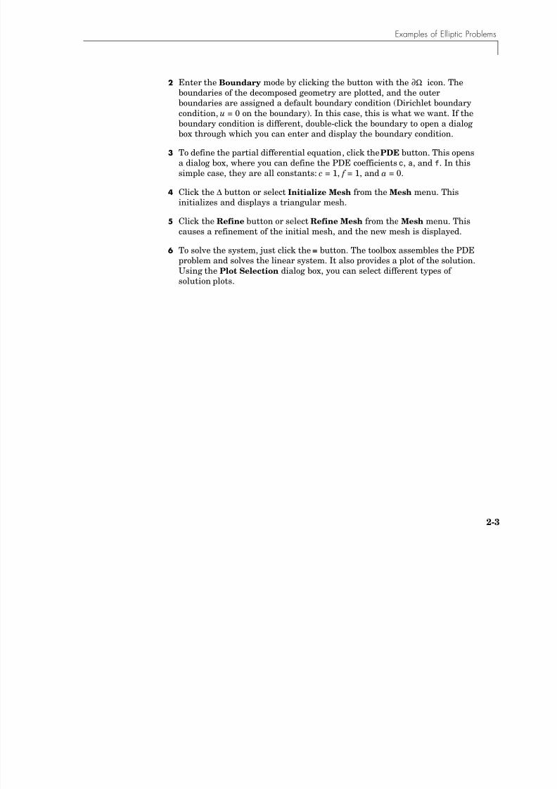
8/21/2019 matlab pde solving.pdf
http://slidepdf.com/reader/full/matlab-pde-solvingpdf 55/290
Examples of Elliptic Problems
2-3
2 Enter the Boundary mode by clicking the button with the icon. Theboundaries of the decomposed geometry are plotted, and the outerboundaries are assigned a default boundary condition (Dirichlet boundarycondition, u = 0 on the boundary). In this case, this is what we want. If theboundary condition is different, double-click the boundary to open a dialogbox through which you can enter and display the boundary condition.
3 To define the partial differential equation, click the PDE button. This opensa dialog box, where you can define the PDE coefficients c, a, and f. In this
simple case, they are all constants: c = 1, f = 1, and a = 0.
4 Click the ∆ button or select Initialize Mesh from the Mesh menu. Thisinitializes and displays a triangular mesh.
5 Click the Refine button or select Refine Mesh from the Mesh menu. Thiscauses a refinement of the initial mesh, and the new mesh is displayed.
6 To solve the system, just click the = button. The toolbox assembles the PDEproblem and solves the linear system. It also provides a plot of the solution.Using the Plot Selection dialog box, you can select different types ofsolution plots.
Ω∂
2 Examples
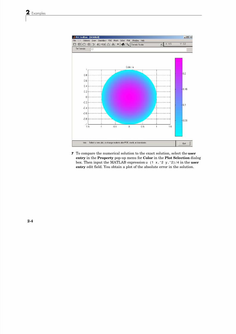
8/21/2019 matlab pde solving.pdf
http://slidepdf.com/reader/full/matlab-pde-solvingpdf 56/290
2-4
7 To compare the numerical solution to the exact solution, select the user
entry in the Property pop-up menu for Color in the Plot Selection dialogbox. Then input the MATLAB expression u (1 x.^2 y.^2)/4 in the user
entry edit field. You obtain a plot of the absolute error in the solution.
Examples of Elliptic Problems
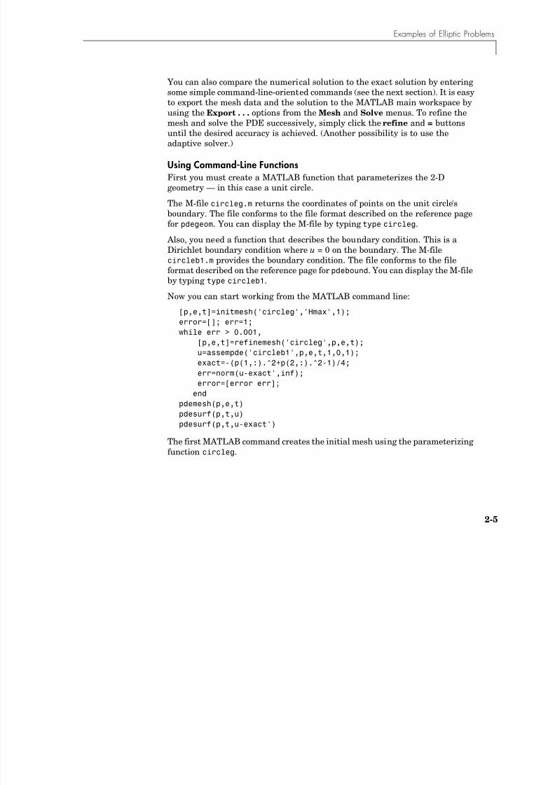
8/21/2019 matlab pde solving.pdf
http://slidepdf.com/reader/full/matlab-pde-solvingpdf 57/290
p p
2-5
You can also compare the numerical solution to the exact solution by enteringsome simple command-line-oriented commands (see the next section). It is easyto export the mesh data and the solution to the MATLAB main workspace byusing the Export . . . options from the Mesh and Solve menus. To refine themesh and solve the PDE successively, simply click the refine and = buttonsuntil the desired accuracy is achieved. (Another possibility is to use theadaptive solver.)
Using Command-Line FunctionsFirst you must create a MATLAB function that parameterizes the 2-Dgeometry — in this case a unit circle.
The M-file circleg.m returns the coordinates of points on the unit circle’ sboundary. The file conforms to the file format described on the reference pagefor pdegeom. You can display the M-file by typing type circleg.
Also, you need a function that describes the boundary condition. This is aDirichlet boundary condition where u = 0 on the boundary. The M-filecircleb1.m provides the boundary condition. The file conforms to the fileformat described on the reference page for pdebound. You can display the M-fileby typing type circleb1.
Now you can start working from the MATLAB command line:
[p,e,t]=initmesh('circleg','Hmax',1);
error=[]; err=1;
while err > 0.001,
[p,e,t]=refinemesh('circleg',p,e,t);
u=assempde('circleb1',p,e,t,1,0,1);
exact=-(p(1,:).^2+p(2,:).^2-1)/4;
err=norm(u-exact',inf);
error=[error err];
end
pdemesh(p,e,t)
pdesurf(p,t,u)
pdesurf(p,t,u-exact')
The first MATLAB command creates the initial mesh using the parameterizingfunction circleg.
2 Examples
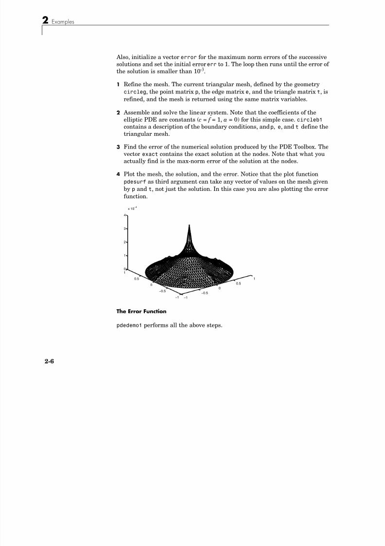
8/21/2019 matlab pde solving.pdf
http://slidepdf.com/reader/full/matlab-pde-solvingpdf 58/290
2-6
Also, initialize a vector error for the maximum norm errors of the successivesolutions and set the initial error err to 1. The loop then runs until the error ofthe solution is smaller than 10-3.
1 Refine the mesh. The current triangular mesh, defined by the geometrycircleg, the point matrix p, the edge matrix e, and the triangle matrix t, isrefined, and the mesh is returned using the same matrix variables.
2 Assemble and solve the linear system. Note that the coefficients of the
elliptic PDE are constants (c = f = 1, a = 0) for this simple case. circleb1 contains a description of the boundary conditions, and p, e, and t define thetriangular mesh.
3 Find the error of the numerical solution produced by the PDE Toolbox. The vector exact contains the exact solution at the nodes. Note that what youactually find is the max-norm error of the solution at the nodes.
4 Plot the mesh, the solution, and the error. Notice that the plot functionpdesurf as third argument can take any vector of values on the mesh givenby p and t, not just the solution. In this case you are also plotting the errorfunction.
The Error Function
pdedemo1 performs all the above steps.
−1−0.5
0
0.5
1
−1
−0.5
0
0.5
1
0
1
2
3
4
x 10−4
Examples of Elliptic Problems
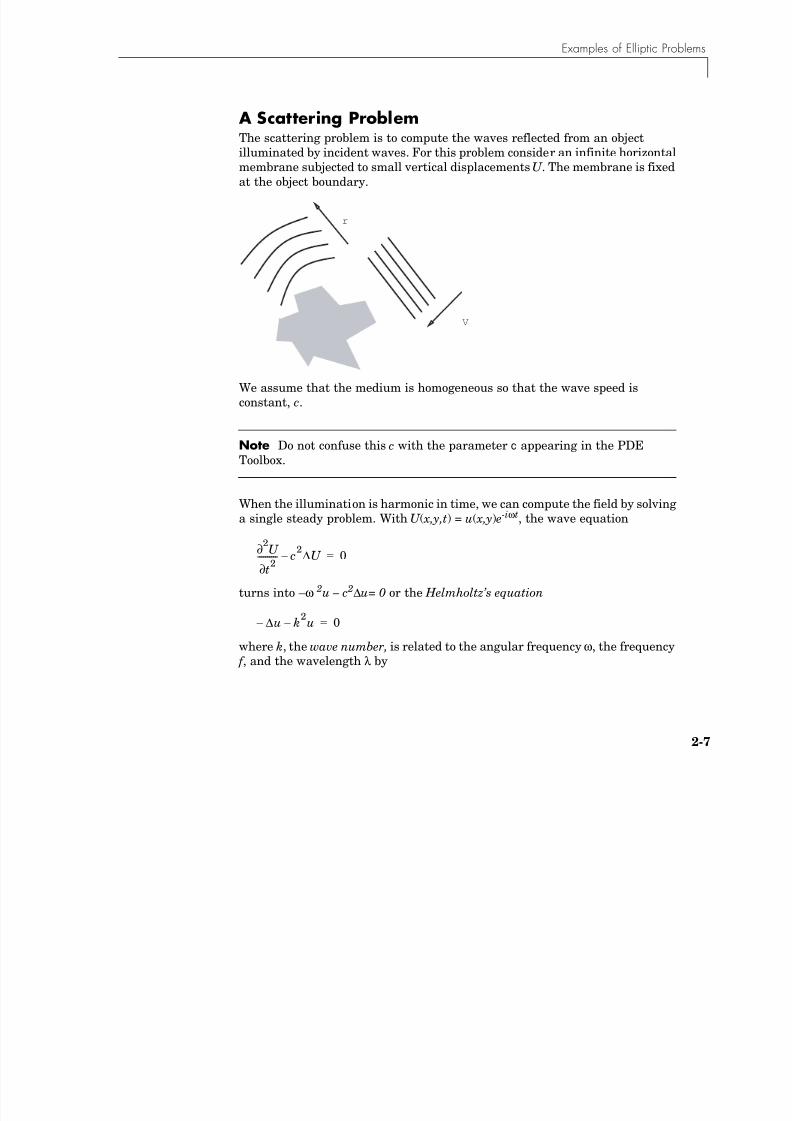
8/21/2019 matlab pde solving.pdf
http://slidepdf.com/reader/full/matlab-pde-solvingpdf 59/290
2-7
A Scattering ProblemThe scattering problem is to compute the waves reflected from an objectilluminated by incident waves. For this problem consider an infinite horizontalmembrane subjected to small vertical displacements U . The membrane is fixedat the object boundary.
We assume that the medium is homogeneous so that the wave speed isconstant, c.
Note Do not confuse this c with the parameter c appearing in the PDEToolbox.
When the illumination is harmonic in time, we can compute the field by solvinga single steady problem. With U ( x,y,t) = u( x,y) e-iωt, the wave equation
turns into –ω 2u – c 2∆u= 0 or the Helmholtz’s equation
where k, the wave number, is related to the angular frequency ω, the frequency f , and the wavelength λ by
r
V
U 2
∂
t∂2
---------- c2
∆U – 0=
∆u – k2u – 0=
2 Examples
8/21/2019 matlab pde solving.pdf
http://slidepdf.com/reader/full/matlab-pde-solvingpdf 60/290
2-8
We have yet to specify the boundary conditions. Let the incident wave be aplane wave traveling in the direction = (cos(a),sin(a))
where
u is the sum of v and the reflected wave r,
u = v + r
The boundary condition for the object’ s boundary is easy: u = 0, i.e.,
r = –v( x, y)
For acoustic waves, where v is the pressure disturbance, the proper conditionwould be
.
The reflected wave r travels outward from the object. The condition at the outercomputational boundary should be chosen to allow waves to pass without
reflection. Such conditions are usually called nonreflecting, and we use theclassical Sommerfeld radiation condition. As approaches infinity, r approximately satisfies the one-way wave equation
which allows waves moving in the positive ξ-direction only (ξ is the radialdistance from the object). With the time-harmonic solution, this turns into the
generalized Neumann boundary condition
For simplicity, let us make the outward normal of the computational domainapproximate the outward ξ-direction.
k ω
c----2π f
c---------2πλ------= = =
a
V x y t, ,( ) ei ka x⋅ ωt – ( )
v x y,( ) eiωt –
= =
v x y,( ) eika x⋅
=
∂u
∂n------ 0=
x
∂r
∂t----- cξ+ ∇r⋅ 0=
ξ ∇r⋅ ikr=
Examples of Elliptic Problems
8/21/2019 matlab pde solving.pdf
http://slidepdf.com/reader/full/matlab-pde-solvingpdf 61/290
2-9
Using the Graphical User Interface You can now use pdetool to solve this scattering problem. Using the Generic
Scalar mode, start by drawing the 2-D geometry of the problem. Let theilluminated object be a square SQ1 with a side of 0.1 units and center in [0.8
0.5] and rotated 45 degrees, and let the computational domain be a circle C1with a radius of 0.45 units and the same center location. The Constructive SolidGeometry (CSG) model is then given by C1 SQ1.
For the outer boundary (the circle perimeter), the boundary condition is a
generalized Neumann condition with q = –ik. The wave number k = 60, whichcorresponds to a wavelength of about 0.1 units, so enter 60i as a constant q and 0 as a constant g.
For the square object’s boundary, you have a Dirichlet boundary condition:
In this problem, the incident wave is traveling in the – x direction, so the
boundary condition is simply
r = – e-ikx
Enter this boundary condition in the Boundary Condition dialog box as aDirichlet condition: h=1, r= exp( i*60*x). The real part of this is a sinusoid.
For sufficient accuracy, about 10 finite elements per wavelength are needed.The outer boundary should be located a few object diameters from the object
itself. An initial mesh generation and two successive mesh refinements giveapproximately the desired resolution.
Although originally a wave equation, the transformation into a Helmholtz’ sequation makes it — in the PDE Toolbox context, but not strictlymathematically — an elliptic equation. The elliptic PDE coefficients for thisproblem are c = 1, a = –k 2 = –3600, and f = 0. Open the PDE Specification dialog box and enter these values.
The problem can now be solved, and the solution is complex. For a complexsolution, the real part is plotted and a warning message is issued.
The propagation of the reflected waves is computed as
Re(r( x,y) e-iωt)
which is the reflex of
r v x y,( ) – e – ika x⋅
= =
2 Examples

8/21/2019 matlab pde solving.pdf
http://slidepdf.com/reader/full/matlab-pde-solvingpdf 62/290
2-10
To see the whole field, plot
The reflected waves and the “shadow” behind the object are clearly visiblewhen you plot the reflected wave.
To make an animation of the reflected wave, the solution and the mesh datamust first be exported to the main workspace. Then make a script M-file or typethe following commands at the MATLAB prompt:
h=newplot; hf=get(h,'Parent'); set(hf,'Renderer','zbuffer')axis tight, set(gca,'DataAspectRatio',[1 1 1]); axis off
M=moviein(10,hf);
maxu=max(abs(u));
colormap(cool)or j=1:10,
ur=real(exp( j*2*pi/10*sqrt( 1))*u));
pdeplot(p,e,t,'xydata',ur,'colorbar','off','mesh','off');
caxis([ maxu maxu]);
axis tight, set(gca,'DataAspectRatio',[1 1 1]); axis off
M(:,j)=getframe;
end
movie(hf,M,50);
pdedemo2 contains a full command-line demonstration of the scatteringproblem.
Re ei k a x⋅ ωt – ( )
)(
Re r x y,( )(( eika x⋅
) eiωt –
)+
Examples of Elliptic Problems
8/21/2019 matlab pde solving.pdf
http://slidepdf.com/reader/full/matlab-pde-solvingpdf 63/290
2-11
A Minimal Surface ProblemIn many problems the coefficients c, a, and f do not only depend on x and y, butalso on the solution u itself. Consider the equation
on the unit disk with on .
This problem is nonlinear and cannot be solved with the regular elliptic solver.Instead, the nonlinear solver pdenonlin is used.
Let us solve this minimal surface problem using the pdetool GUI andcommand-line functions.
Using the Graphical User InterfaceMake sure that the application mode in the pdetool GUI is set to Generic
Scalar. The problem domain is simply a unit circle. Draw it and move to theBoundary mode to define the boundary conditions. Use Select All from theEdit menu to select all boundaries. Then double-click a boundary to open theBoundary Condition dialog box. The Dirichlet condition u = x 2 is entered bytyping x.^2 into the r edit box. Next, open the PDE Specification dialog boxto define the PDE. This is an elliptic equation with
The nonlinear c is entered into the c edit box as
1./sqrt(1+ux.^2+uy.^2)
Initialize a mesh and refine it once.
Before solving the PDE, select Parameters . . . from the Solve menu and checkthe Use nonlinear solver option. Also, set the tolerance parameter to 0.001.
Click the = button to solve the PDE. Use the Plot Selection dialog box to plotthe solution in 3-D (check u and continuous selections in the Height column)to visualize the saddle shape of the solution.
∇ – 1
1 ∇u2
+
----------------------------∇u# $% &' (
⋅ 0=
Ω x y( , ) x2
y2 1≤+ = u x
2= ∂Ω
c1
1 ∇u 2+
---------------------------- a 0,= and f 0=,=
2 Examples
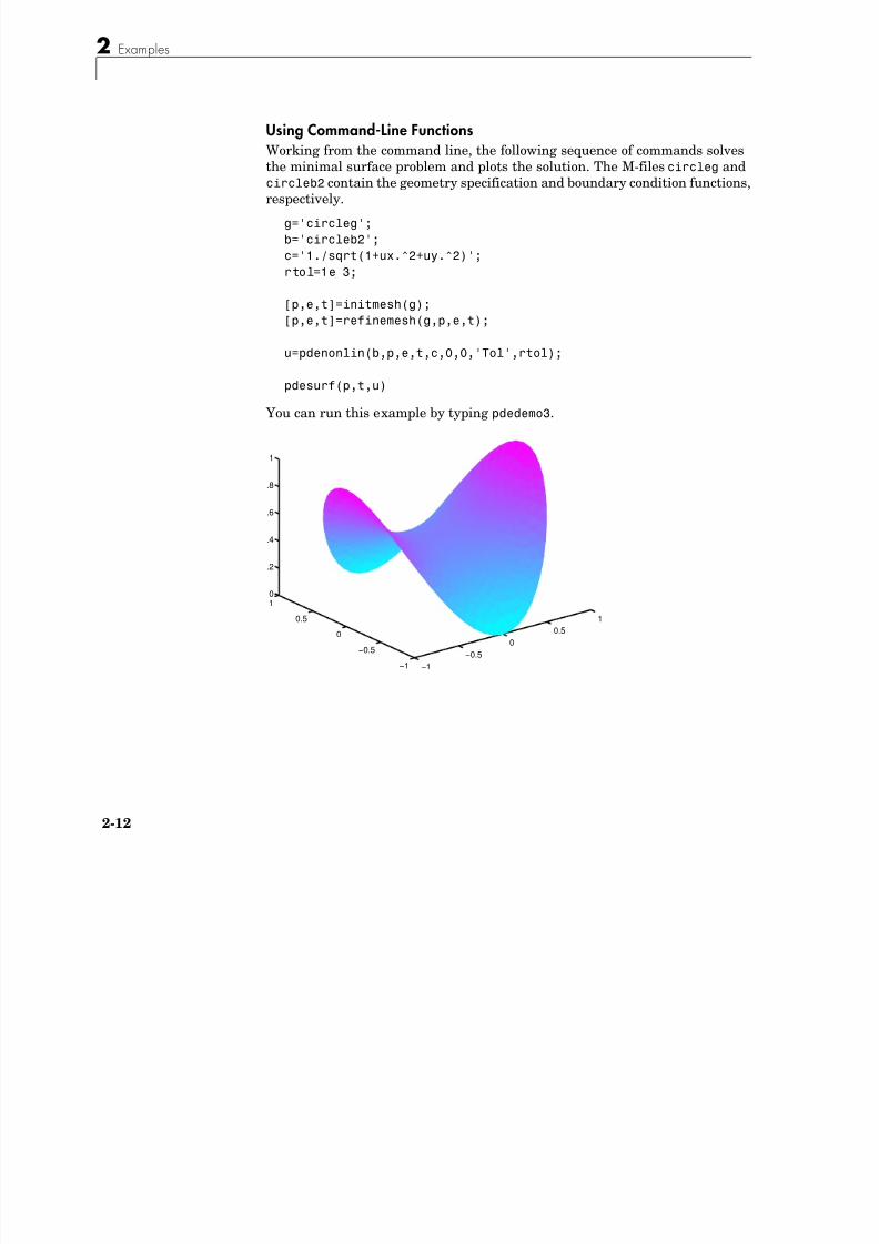
8/21/2019 matlab pde solving.pdf
http://slidepdf.com/reader/full/matlab-pde-solvingpdf 64/290
2-12
Using Command-Line FunctionsWorking from the command line, the following sequence of commands solvesthe minimal surface problem and plots the solution. The M-files circleg andcircleb2 contain the geometry specification and boundary condition functions,respectively.
g='circleg';
b='circleb2';
c='1./sqrt(1+ux.^2+uy.^2)';
rtol=1e 3;
[p,e,t]=initmesh(g);
[p,e,t]=refinemesh(g,p,e,t);
u=pdenonlin(b,p,e,t,c,0,0,'Tol',rtol);
pdesurf(p,t,u)
You can run this example by typing pdedemo3.
−
1
−0.5
0
0.5
1
−
1
−0.5
0
0.5
10
.2
.4
.6
.8
1
Examples of Elliptic Problems
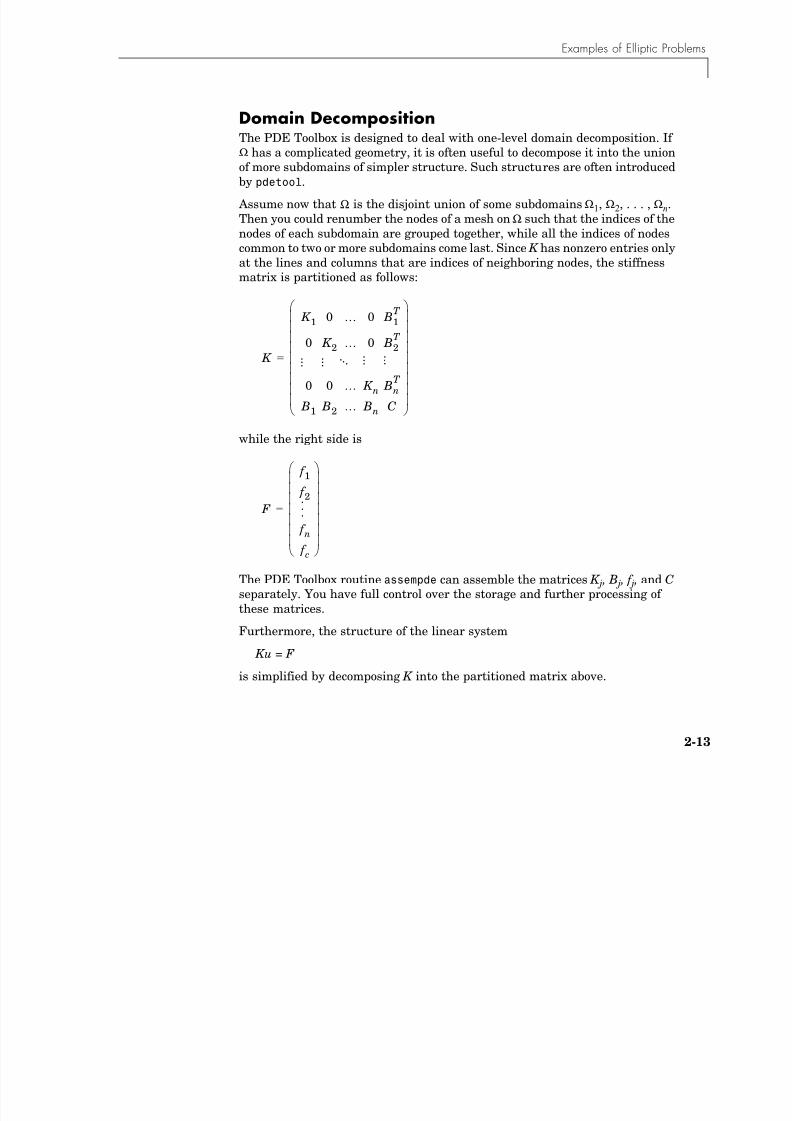
8/21/2019 matlab pde solving.pdf
http://slidepdf.com/reader/full/matlab-pde-solvingpdf 65/290
2-13
Domain DecompositionThe PDE Toolbox is designed to deal with one-level domain decomposition. IfΩ has a complicated geometry, it is often useful to decompose it into the unionof more subdomains of simpler structure. Such structures are often introducedby pdetool.
Assume now that Ω is the disjoint union of some subdomains Ω1, Ω2, . . . , Ωn.Then you could renumber the nodes of a mesh on Ω such that the indices of thenodes of each subdomain are grouped together, while all the indices of nodes
common to two or more subdomains come last. Since K has nonzero entries onlyat the lines and columns that are indices of neighboring nodes, the stiffnessmatrix is partitioned as follows:
while the right side is
The PDE Toolbox routine assempde can assemble the matrices K j , B j , f j , and C separately. You have full control over the storage and further processing ofthese matrices.
Furthermore, the structure of the linear system
Ku = F
is simplified by decomposing K into the partitioned matrix above.
K
K 1 0 … 0 B1T
0 K 2 … 0 B2T
0 0 … K n BnT
B1 B2 … Bn C# $% &% &% &% &% &% &% &% &% &' (
=
.
.
.
.
.
.
. .
.
.
.
.
.
.
.
F
f 1
f 2
f n
f c# $% &% &% &% &% &% &% &' (
= .
.
.
2 Examples
8/21/2019 matlab pde solving.pdf
http://slidepdf.com/reader/full/matlab-pde-solvingpdf 66/290
2-14
Now consider the geometry of the L-shaped membrane. You can plot the
geometry of the membrane by typingpdegplot('lshapeg')
Notice the borders between the subdomains. There are three subdomains. Thusthe matrix formulas with n = 3 from above can be used. Now generate a meshfor the geometry:
[p,e,t]=initmesh('lshapeg');
[p,e,t]=refinemesh('lshapeg',p,e,t);[p,e,t]=refinemesh('lshapeg',p,e,t);
So for this case, with n = 3, you have
and the solution is given by block elimination:
K 1 0 0 B1T
0 K 2 0 B2T
0 0 K 3 B3T
B1 B2 B3 C# $% &% &% &
% &% &% &% &' (
u1
u2
u3uc# $
% &% &% &
% &% &% &' (
f 1
f 2
f 3 f c# $
% &% &% &
% &% &% &' (
=
C B1 K 11 – B1
T – B2 K 2
1 – B2
T – B3 K 3
1 – B3
T – ( )uc f c B1 K 1
1 – f 1 – B2 K 2
1 – f 2 – B3 K 3
1 – f 3 – =
u1 K 11 –
f 1 B1T
uc – ( )=
…
Examples of Elliptic Problems

8/21/2019 matlab pde solving.pdf
http://slidepdf.com/reader/full/matlab-pde-solvingpdf 67/290
2-15
In the MATLAB solution below, a more efficient algorithm using Choleski
factorization is used:time=[];
np=size(p,2);
% Find common points
c=pdesdp(p,e,t);
nc=length(c);
C=zeros(nc,nc);FC=zeros(nc,1);
[i1,c1]=pdesdp(p,e,t,1);ic1=pdesubix(c,c1);
[K,F]=assempde('lshapeb',p,e,t,1,0,1,time,1);
K1=K(i1,i1);d=symmmd(K1);i1=i1(d);
K1=chol(K1(d,d));B1=K(c1,i1);a1=B1/K1;
C(ic1,ic1)=C(ic1,ic1)+K(c1,c1) a1*a1';
f1=F(i1);e1=K1'\f1;FC(ic1)=FC(ic1)+F(c1) a1*e1;
[i2,c2]=pdesdp(p,e,t,2);ic2=pdesubix(c,c2);
[K,F]=assempde('lshapeb',p,e,t,1,0,1,time,2);
K2=K(i2,i2);d=symmmd(K2);i2=i2(d);
K2=chol(K2(d,d));B2=K(c2,i2);a2=B2/K2;
C(ic2,ic2)=C(ic2,ic2)+K(c2,c2) a2*a2';
f2=F(i2);e2=K2'\f2;FC(ic2)=FC(ic2)+F(c2) a2*e2;
[i3,c3]=pdesdp(p,e,t,3);ic3=pdesubix(c,c3);
[K,F]=assempde('lshapeb',p,e,t,1,0,1,time,3);
K3=K(i3,i3);d=symmmd(K3);i3=i3(d);
K3=chol(K3(d,d));B3=K(c3,i3);a3=B3/K3;
C(ic3,ic3)=C(ic3,ic3)+K(c3,c3) a3*a3';
f3=F(i3);e3=K3'\f3;FC(ic3)=FC(ic3)+F(c3) a3*e3;
% Solve
u=zeros(np,1);u(c)=C\ FC;
u(i1)=K1\(e1 a1'*u(c1));
u(i2)=K2\(e2 a2'*u(c2));
u(i3)=K3\(e3 a3'*u(c3));
2 Examples
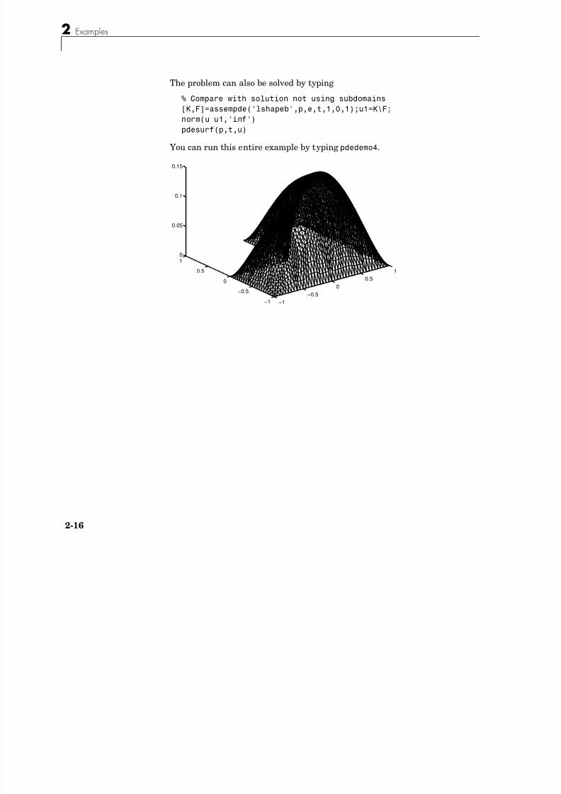
8/21/2019 matlab pde solving.pdf
http://slidepdf.com/reader/full/matlab-pde-solvingpdf 68/290
2-16
The problem can also be solved by typing
% Compare with solution not using subdomains
[K,F]=assempde('lshapeb',p,e,t,1,0,1);u1=K\F;
norm(u u1,'inf')
pdesurf(p,t,u)
You can run this entire example by typing pdedemo4.
−1
−0.5
0
0.5
1
−1
−0.5
0
0.5
1
0
0.05
0.1
0.15
Examples of Parabolic Problems
8/21/2019 matlab pde solving.pdf
http://slidepdf.com/reader/full/matlab-pde-solvingpdf 69/290
2-17
Examples of Parabolic ProblemsThis section describes the solution of some parabolic PDE problems. Theproblems are solved using both the graphical user interface and thecommand-line functions of the PDE Toolbox. The topics include
• “The Heat Equation: A Heated Metal Block”
• “Heat Distribution in Radioactive Rod” on page 2-21
The Heat Equation: A Heated Metal Block A common parabolic problem is the heat equation:
The heat equation describes the diffusion of heat in a body of some kind. Seethe section “Application Modes” on page 2-37 for more information about heat
transfer and diffusion problems.This first example studies a heated metal block with a rectangular crack orcavity. The left side of the block is heated to 100 degrees centigrade. At theright side of the metal block, heat is flowing from the block to the surroundingair at a constant rate. All the other block boundaries are isolated. This leads tothe following set of boundary conditions (when proper scaling of t is chosen):
• on the left side (Dirichlet condition)
• on the right side (Neumann condition)
• on all other boundaries (Neumann condition)
Also, for the heat equation we need an initial value: the temperature in themetal block at the starting time t0. In this case, the temperature of the block is0 degrees at the time we start applying heat.
Finally, to complete the problem formulation, we specify that the starting time
is 0 and that we want to study the heat distribution during the first fiveseconds.
d∂u
∂t------ ∆u – 0=
u 100=
∂u∂n------ 10 – =∂u
∂n------ 0=
2 Examples
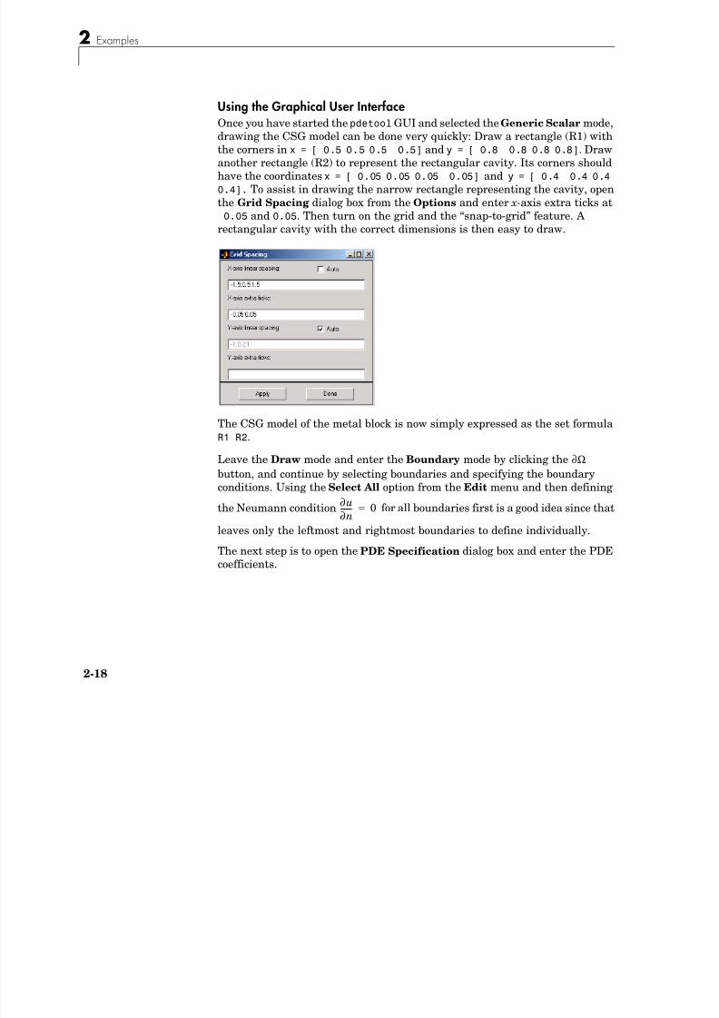
8/21/2019 matlab pde solving.pdf
http://slidepdf.com/reader/full/matlab-pde-solvingpdf 70/290
2-18
Using the Graphical User InterfaceOnce you have started the pdetool GUI and selected the Generic Scalar mode,drawing the CSG model can be done very quickly: Draw a rectangle (R1) withthe corners in x = [ 0.5 0.5 0.5 0.5] and y = [ 0.8 0.8 0.8 0.8]. Drawanother rectangle (R2) to represent the rectangular cavity. Its corners shouldhave the coordinates x = [ 0.05 0.05 0.05 0.05] and y = [ 0.4 0.4 0.4
0.4]. To assist in drawing the narrow rectangle representing the cavity, openthe Grid Spacing dialog box from the Options and enter x-axis extra ticks at0.05 and 0.05. Then turn on the grid and the “snap-to-grid” feature. A
rectangular cavity with the correct dimensions is then easy to draw.
The CSG model of the metal block is now simply expressed as the set formula
R1 R2.Leave the Draw mode and enter the Boundary mode by clicking thebutton, and continue by selecting boundaries and specifying the boundaryconditions. Using the Select All option from the Edit menu and then defining
the Neumann condition for all boundaries first is a good idea since that
leaves only the leftmost and rightmost boundaries to define individually.
The next step is to open the PDE Specification dialog box and enter the PDEcoefficients.
Ω∂
∂u
∂n------ 0=
Examples of Parabolic Problems
8/21/2019 matlab pde solving.pdf
http://slidepdf.com/reader/full/matlab-pde-solvingpdf 71/290
2-19
The generic parabolic PDE that the PDE Toolbox solves is
with initial values u0 = u(t0) and the times at which to compute a solutionspecified in the array tlist.
For this case, you have d = 1, c = 1, a = 0, and f = 0.
Initialize the mesh by clicking the ∆ button. If you want, you can refine themesh by clicking the Refine button.
The initial values u0 = 0, and the list of times is entered as the MATLAB array[0:0.5:5]. They are entered into the Solve Parameters dialog box, which isaccessed by selecting Parameters . . . from the Solve menu.
The problem can now be solved. Pressing the = button solves the heat equationat 11 different times from 0 to 5 seconds. By default, an interpolated plot of thesolution, i.e., the heat distribution, at the end of the time span is displayed.
A more interesting way to visualize the dynamics of the heat distributionprocess is to animate the solution. To start an animation, check the Animation check box in the Plot selection dialog box. Also, select the colormap hot. Clickthe Plot button to start a recording of the solution plots in a separate figurewindow. The recorded animation is then “played” five times.
Note that the temperature in the block rises very quickly. To improve theanimation and focus on the first second, try to change the list of times to theMATLAB expression logspace( 2,0.5,20).
du∂t∂
------ ∇ – c∇u( )⋅ au+ f =
2 Examples

8/21/2019 matlab pde solving.pdf
http://slidepdf.com/reader/full/matlab-pde-solvingpdf 72/290
2-20
Also, try to change the heat capacity coefficient d and the heat flow at the
rightmost boundary to see how they affect the heat distribution.
Using Command-Line FunctionsFirst, you must create geometry and boundary condition M-files. The M-filesused here were created using pdetool. The geometry of the metal block isdescribed in crackg.m, and the boundary conditions can be found in crackb.m.
To create an initial mesh, call initmesh:
» [p,e,t]=initmesh('crackg');
The heat equation can now be solved using the PDE Toolbox functionparabolic. The generic parabolic PDE that parabolic solves is
with initial value u0 = u(t0 ) and the times at which to compute a solutionspecified in the array tlist. For this case, you have d = 1, c = 1, a = 0, and f = 0.The initial value u0 = 0, and the list of times, tlist, is set to the MATLABarray 0:0.5:5.
du∂
t∂
------ ∇ – c∇u( )⋅ au+ f =
Examples of Parabolic Problems
8/21/2019 matlab pde solving.pdf
http://slidepdf.com/reader/full/matlab-pde-solvingpdf 73/290
2-21
To compute the solution, call parabolic:
u=parabolic(0,0:0.5:5,'crackb',p,e,t,1,0,0,1);
The solution u created this way a matrix with 11 columns, where each columncorresponds to the solution at the 11 points in time 0,0.5, . . . ,4.5,5.0.
Let us plot the solution at t = 5.0 seconds using interpolated shading and ahidden mesh. Use the hot colormap:
pdeplot(p,e,t,'xydata',u(:,11),'mesh','off',...
'colormap','hot')
Heat Distribution in Radioactive RodThis heat distribution problem is an example of a 3-D parabolic PDE problemthat is reduced to a 2-D problem by using cylindrical coordinates.
Consider a cylindrical radioactive rod. At the left end, heat is continuously
added. The right end is kept at a constant temperature. At the outer boundary,heat is exchanged with the surroundings by transfer. At the same time, heat isuniformly produced in the whole rod due to radioactive processes. Assume thatthe initial temperature is zero. This leads to the following problem:
where ρ is the density, C is the rod’s thermal capacity, k is the thermalconductivity, and f is the radioactive heat source.
The density for this metal rod is 7800 kg/m3, the thermal capacity is500 Ws/kg°C, and the thermal conductivity is 40 W/m°C. The heat source is20000 W/m3. The temperature at the right end is 100 °C. The surroundingtemperature at the outer boundary is 100 °C, and the heat transfer coefficientis 50 W/m2°C. The heat flux at the left end is 5000 W/m2.
But this is a cylindrical problem, so you need to transform the equation, using
the cylindrical coordinates r, z, and θ. Due to symmetry, the solution isindependent of θ, so the transformed equation is
ρCu∂t∂
------ ∇ – k∇u( )⋅ f =
rρC∂u
∂t------
r∂∂
kr∂u
∂r------
# $' ( –
z∂∂
kr∂u
∂ z------
# $' ( – fr=
2 Examples
8/21/2019 matlab pde solving.pdf
http://slidepdf.com/reader/full/matlab-pde-solvingpdf 74/290
2-22
The boundary conditions are
• = 5000 at the left end of the rod (Neumann condition). Since thegeneralized Neumann condition in the PDE Toolbox is + qu = g,and c depends on r in this problem (c = kr), this boundary condition isexpressed as = 5000r
•u = 100 at the right end of the rod (Dirichlet condition).
• = 50(100-u) at the outer boundary (generalized Neumanncondition). In the PDE toolbox this must be expressed as
+ 50r ⋅ u = 50r ⋅ 100.•The cylinder axis r = 0 is not a boundary in the original problem, but in our
2-D treatment it has become one. We must give the artificial boundarycondition here.
The initial value is u(t0) = 0.
Using the Graphical User InterfaceSolve this problem using the pdetool GUI. Model the rod as a rectangle withits base along the x-axis, and let the x-axis be the z direction and the y-axis bethe r direction. A rectangle with corners in (-1.5,0), (1.5,0), (1.5,0.2), and(-1.5,0.2) would then model a rod with length 3 and radius 0.2.
Enter the boundary conditions by double-clicking the boundaries to open theBoundary Condition dialog box. For the left end, use Neumann conditionswith 0 for q and 5000*y for g. For the right end, use Dirichlet conditions with 1
for h and 100 for r. For the outer boundary, use Neumann conditions with 50*y for q and 50*y*100 for g. For the axis, use Neumann conditions with 0 for q and g.
Enter the coefficients into the PDE Specification dialog box: c is 40*y, a iszero, d is 7800*500*y, and f is 20000*y.
Animate the solution over a span of 20000 seconds (computing the solutionevery 1000 seconds). We can see how heat flows in over the right and outer
boundaries as long as u < 100, and out when u > 100. You can also open thePDE Specification dialog box, and change the PDE type to Elliptic. Thisshows the solution when u does not depend on time, i.e., the steady statesolution. The profound effect of cooling on the outer boundary can bedemonstrated by setting the heat transfer coefficient to zero.
n k∇u( )⋅
n c∇u( )⋅
n c∇u( )⋅
n k∇u( )⋅
n c∇u( )⋅
n c∇u( )⋅ 0=
Example of a Hyperbolic Problem
8/21/2019 matlab pde solving.pdf
http://slidepdf.com/reader/full/matlab-pde-solvingpdf 75/290
2-23
Example of a Hyperbolic ProblemThis section describes the solution of a hyperbolic PDE problem. The problemis solved using the graphical user interface (GUI) and the command-linefunctions of the PDE Toolbox.
The Wave Equation As an example of a hyperbolic PDE, let us solve the wave equation
for transverse vibrations of a membrane on a square with corners in (-1,-1),(-1,1), (1,-1), and (1,1). The membrane is fixed (u = 0) at the left and right sides,and is free
at the upper and lower sides. Additionally, we need initial values for
u(t0) and
The initial values need to match the boundary conditions for the solution to be
well-behaved. If we start at t=0,
and
are initial values that satisfy the boundary conditions. The reason for thearctan and exponential functions is to introduce more modes into the solution.
∂2u
∂t2
--------- ∆u – 0=
∂u∂n------ 0=# $' (
∂u t0( )
∂t-----------------
u 0( ) π
2--- x# $
' (cos# $' (atan=
∂u 0( )
∂t
--------------- 3 π x( ) e
π2--- y) *sin
sin=
2 Examples
8/21/2019 matlab pde solving.pdf
http://slidepdf.com/reader/full/matlab-pde-solvingpdf 76/290
2-24
Using the Graphical User Interface
Use the pdetool GUI in the Generic Scalar mode. Draw the square using theRectangle/square option from the Draw menu or the button with therectangle icon. Proceed to define the boundary conditions by clicking thebutton and then double-click the boundaries to define the boundary conditions.
Initialize the mesh by clicking the ∆ button or by selecting Initialize mesh from the Mesh menu.
Also, define the hyperbolic PDE by opening the PDE Specification dialog box,selecting the hyperbolic PDE, and entering the appropriate coefficient values.The general hyperbolic PDE is described by
so for the wave equation you get c = 1, a = 0, f = 0, and d = 1.
Before solving the PDE, select Parameters . . . from the Solve menu to openthe Solve Parameters dialog box. As a list of times, enter linspace(0,5,31) and as initial values for u:
atan(cos(pi/2*x))
and for , enter
3*sin(pi*x).*exp(sin(pi/2*y))
Ω∂
d∂
2u
∂t2
--------- ∇ – c∇u( )⋅ au+ f =
∂u
∂t------
Example of a Hyperbolic Problem
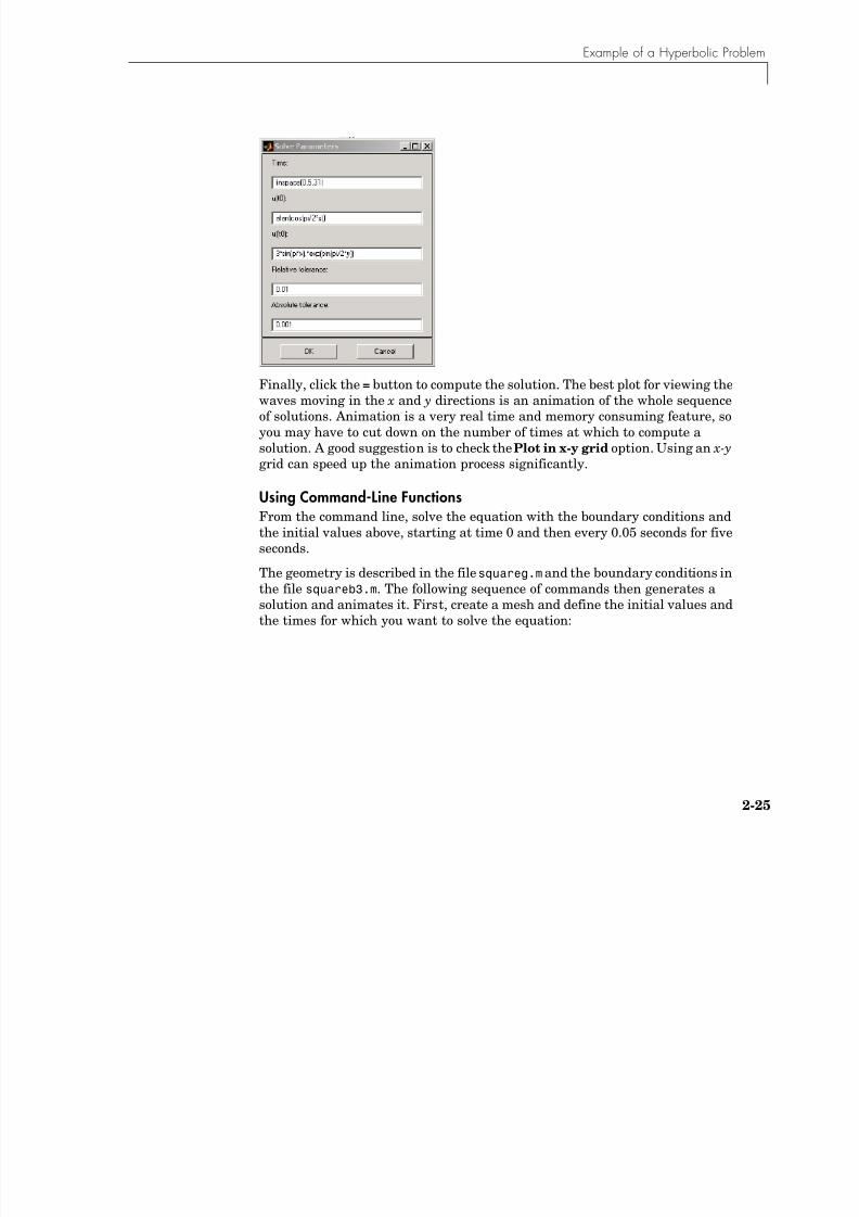
8/21/2019 matlab pde solving.pdf
http://slidepdf.com/reader/full/matlab-pde-solvingpdf 77/290
2-25
Finally, click the = button to compute the solution. The best plot for viewing the
waves moving in the x and y directions is an animation of the whole sequenceof solutions. Animation is a very real time and memory consuming feature, soyou may have to cut down on the number of times at which to compute asolution. A good suggestion is to check the Plot in x-y grid option. Using an x-y grid can speed up the animation process significantly.
Using Command-Line FunctionsFrom the command line, solve the equation with the boundary conditions and
the initial values above, starting at time 0 and then every 0.05 seconds for fiveseconds.
The geometry is described in the file squareg.m and the boundary conditions inthe file squareb3.m. The following sequence of commands then generates asolution and animates it. First, create a mesh and define the initial values andthe times for which you want to solve the equation:
2 Examples
8/21/2019 matlab pde solving.pdf
http://slidepdf.com/reader/full/matlab-pde-solvingpdf 78/290
2-26
[p,e,t]=initmesh('squareg');
x=p(1,:)'; y=p(2,:)';
u0=atan(cos(pi/2*x));
ut0=3*sin(pi*x).*exp(sin(pi/2*y));
n=31;
tlist=linspace(0,5,n); % list of times
You are now ready to solve the wave equation. The general form for thehyperbolic PDE in the PDE Toolbox is
so here you have d = 1, c = 1, a = 0, and f = 0:
uu=hyperbolic(u0,ut0,tlist,'squareb3',p,e,t,1,0,0,1);
To visualize the solution, you can animate it. Interpolate to a rectangular gridto speed up the plotting:
delta= 1:0.1:1;
[uxy,tn,a2,a3]=tri2grid(p,t,uu(:,1),delta,delta);
gp=[tn;a2;a3];
umax=max(max(uu));umin=min(min(uu));
newplot
M=moviein(n);
for i=1:n,
pdeplot(p,e,t,'xydata',uu(:,i),'zdata',uu(:,i),...
'mesh','off','xygrid','on','gridparam',gp,...
'colorbar','off','zstyle','continuous');axis([ 1 1 1 1 umin umax]); caxis([umin umax]);
M(:,i)=getframe;
end
movie(M,10);
d∂
2u
∂t2
--------- ∇ – c∇u( )⋅ au+ f =
Example of a Hyperbolic Problem

8/21/2019 matlab pde solving.pdf
http://slidepdf.com/reader/full/matlab-pde-solvingpdf 79/290
2-27
You can find a complete demo of this problem, including animation, inpdedemo6. If you have lots of memory, you can try increasing n, the number offrames in the movie.
Animation of the Solution to the Wave Equation
2 Examples
8/21/2019 matlab pde solving.pdf
http://slidepdf.com/reader/full/matlab-pde-solvingpdf 80/290
2-28
Examples of Eigenvalue Problems
This section describes the solution of some eigenvalue PDE problems. Theproblems are solved using the graphical user interface (GUI) and thecommand-line functions of the PDE Toolbox. The problems include
• “Eigenvalues and Eigenfunctions for the L-Shaped Membrane”
• “L-Shaped Membrane with Rounded Corner” on page 2-32
• “Eigenvalues and Eigenmodes of a Square” on page 2-34
Eigenvalues and Eigenfunctions for the L-ShapedMembraneThe problem of finding the eigenvalues and the corresponding eigenfunctionsof an L-shaped membrane is of interest to all MATLAB users, since the plot ofthe first eigenfunction is the logo of The MathWorks. In fact, you can comparethe PDE Toolbox computed eigenvalues and eigenfunctions to the ones
produced by the MATLAB function membrane.The problem is to compute all eigenmodes with eigenvalues < 100 for the eigenmode PDE problem
–∆u = λu
on the geometry of the L-shaped membrane. u = 0 on the boundary (Dirichletcondition).
Using the Graphical User InterfaceWith the pdetool GUI active, check that the current mode is Generic Scalar.Then draw the L-shape as a polygon with corners in (0,0), (-1,0), (-1,-1), (1,-1),(1,1), and (0,1).
There is no need to define any boundary conditions for this problem since thedefault condition — u = 0 on the boundary — is the correct one. Therefore, youcan continue to the next step: to initialize the mesh. Refine the initial meshtwice. Defining the eigenvalue PDE problem is also easy. Open the PDE
Specification dialog box and select Eigenmodes. The default values for thePDE coefficients, c = 1, a = 0, d = 1, all match the problem description, so youcan exit the PDE Specification dialog box by clicking the OK button.
Examples of Eigenvalue Problems
8/21/2019 matlab pde solving.pdf
http://slidepdf.com/reader/full/matlab-pde-solvingpdf 81/290
2-29
Open the Solve Parameters dialog box by selecting Parameters . . . from theSolve menu. The dialog box contains an edit box for entering the eigenvaluesearch range. The default entry is [0 100], which is just what you want.
Finally, solve the L-shaped membrane problem by clicking the = button. Thesolution displayed is the first eigenfunction. The value of the first (smallest)eigenvalue is also displayed. You find the number of eigenvalues on theinformation line at the bottom of the GUI. You can open the Plot Selection dialog box and choose which eigenfunction to plot by selecting from a pop-upmenu of the corresponding eigenvalues.
Using Command-Line FunctionsThe geometry of the L-shaped membrane is described in the file lshapeg.m andthe boundary conditions in the file lshapeb.m.
First, initialize the mesh and refine it twice using the command line functionsat the MATLAB prompt:
[p,e,t]=initmesh('lshapeg');[p,e,t]=refinemesh('lshapeg',p,e,t);
[p,e,t]=refinemesh('lshapeg',p,e,t);
Recall the general eigenvalue PDE problem description:
This means that in this case you have c = 1, a = 0, and d = 1. The syntax of
pdeeig, the eigenvalue solver in the PDE Toolbox, is[v,l]=pdeeig(b,p,e,t,c,a,d,r)
The input argument r is a two-element vector indicating the interval on thereal axis where pdeeig searches for eigenvalues. Here you are looking foreigenvalues < 100, so the interval you use is [0 100].
Now you can call pdeeig and see how many eigenvalues you find:
[v,l]=pdeeig('lshapeb',p,e,t,1,0,1,[0 100]);
∇ – c∇u( )⋅ au+ λdu=
2 Examples
8/21/2019 matlab pde solving.pdf
http://slidepdf.com/reader/full/matlab-pde-solvingpdf 82/290
2-30
There are 19 eigenvalues smaller than 100. Plot the first eigenmode and
compare it to the MATLAB membrane function:pdesurf(p,t,v(:,1))
figure
membrane(1,20,9,9)
membrane can produce the first 12 eigenfunctions for the L-shaped membrane.Compare also the 12th eigenmodes:
figurepdesurf(p,t,v(:,12))
figure
membrane(12,20,9,9)
Looking at the following eigenmodes, you can see how the number ofoscillations increases. The eigenfunctions are symmetric or antisymmetricaround the diagonal from (0,0) to (1,-1), which divides the L-shaped membraneinto two mirror images. In a practical computation, you could take advantage
of such symmetries in the PDE problem, and solve over a region half the size.The eigenvalues of the full L-shaped membrane are the union of those of thehalf with Dirichlet boundary condition along the diagonal (eigenvalues 2, 4, 7,11, 13, 16, and 17) and those with Neumann boundary condition (eigenvalues1, 3, 5, 6, 10, 12, 14, and 15).
The eigenvalues λ8 and λ9 make up a double eigenvalue for the PDE at around49.64. Also, the eigenvalues λ18 and λ19 make up another double eigenvalue at
around 99.87. You may have gotten two different but close values. The defaulttriangulation made by initmesh is not symmetric around the diagonal, but asymmetric grid gives a matrix with a true double eigenvalue. Each of theeigenfunctions u8 and u9 consists of three copies of eigenfunctions over the unitsquare, corresponding to its double second eigenvalue. You may not haveobtained the zero values along a diagonal of the square — any line through thecenter of the square may have been computed. This shows a general fact aboutmultiple eigenvalues for symmetric matrices; namely that any vector in theinvariant subspace is equally valid as an eigenvector. The two eigenfunctionsu8 and u9 are orthogonal to each other if the dividing lines make right angles.Check your solutions for that.
Examples of Eigenvalue Problems
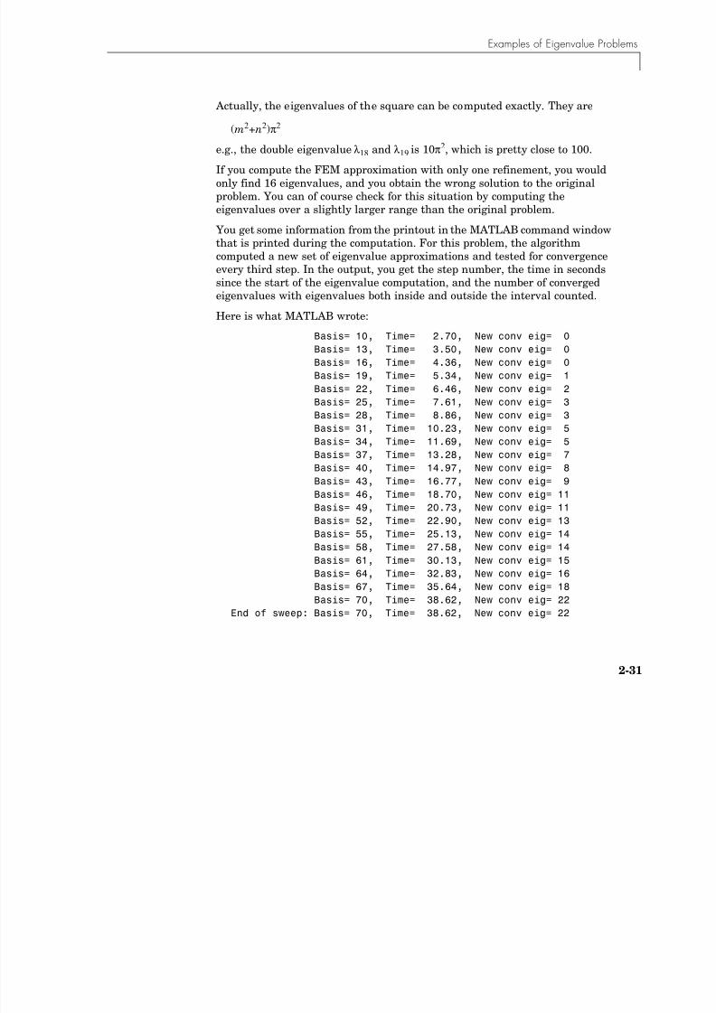
8/21/2019 matlab pde solving.pdf
http://slidepdf.com/reader/full/matlab-pde-solvingpdf 83/290
2-31
Actually, the eigenvalues of the square can be computed exactly. They are
(m2+n2)π2
e.g., the double eigenvalue λ18 and λ19 is 10π2, which is pretty close to 100.
If you compute the FEM approximation with only one refinement, you wouldonly find 16 eigenvalues, and you obtain the wrong solution to the originalproblem. You can of course check for this situation by computing theeigenvalues over a slightly larger range than the original problem.
You get some information from the printout in the MATLAB command windowthat is printed during the computation. For this problem, the algorithmcomputed a new set of eigenvalue approximations and tested for convergenceevery third step. In the output, you get the step number, the time in secondssince the start of the eigenvalue computation, and the number of convergedeigenvalues with eigenvalues both inside and outside the interval counted.
Here is what MATLAB wrote:
Basis= 10, Time= 2.70, New conv eig= 0Basis= 13, Time= 3.50, New conv eig= 0
Basis= 16, Time= 4.36, New conv eig= 0
Basis= 19, Time= 5.34, New conv eig= 1
Basis= 22, Time= 6.46, New conv eig= 2
Basis= 25, Time= 7.61, New conv eig= 3
Basis= 28, Time= 8.86, New conv eig= 3
Basis= 31, Time= 10.23, New conv eig= 5
Basis= 34, Time= 11.69, New conv eig= 5Basis= 37, Time= 13.28, New conv eig= 7
Basis= 40, Time= 14.97, New conv eig= 8
Basis= 43, Time= 16.77, New conv eig= 9
Basis= 46, Time= 18.70, New conv eig= 11
Basis= 49, Time= 20.73, New conv eig= 11
Basis= 52, Time= 22.90, New conv eig= 13
Basis= 55, Time= 25.13, New conv eig= 14
Basis= 58, Time= 27.58, New conv eig= 14Basis= 61, Time= 30.13, New conv eig= 15
Basis= 64, Time= 32.83, New conv eig= 16
Basis= 67, Time= 35.64, New conv eig= 18
Basis= 70, Time= 38.62, New conv eig= 22
End of sweep: Basis= 70, Time= 38.62, New conv eig= 22
2 Examples
8/21/2019 matlab pde solving.pdf
http://slidepdf.com/reader/full/matlab-pde-solvingpdf 84/290
2-32
Basis= 32, Time= 43.29, New conv eig= 0
Basis= 35, Time= 44.70, New conv eig= 0Basis= 38, Time= 46.22, New conv eig= 0
Basis= 41, Time= 47.81, New conv eig= 0
Basis= 44, Time= 49.52, New conv eig= 0
Basis= 47, Time= 51.35, New conv eig= 0
Basis= 50, Time= 53.27, New conv eig= 0
Basis= 53, Time= 55.30, New conv eig= 0
End of sweep: Basis= 53, Time= 55.30, New conv eig= 0
You can see that two Arnoldi runs were made. In the first, 22 eigenvaluesconverged after a basis of size 70 was computed; in the second, where the vectors were orthogonalized against all the 22 converged vectors, the smallesteigenvalue stabilized at a value outside of the interval [0, 100], so the algorithmsignaled convergence. Of the 22 converged eigenvalues, 19 were inside thesearch interval.
L-Shaped Membrane with Rounded Corner An extension of this problem is to compute the eigenvalues for an L-shapedmembrane where the inner corner at the “knee” is rounded. The roundness iscreated by adding a circle so that the circle ’ s arc is a part of the L-shapedmembrane’ s boundary. By varying the circle’ s radius, the degree of roundnesscan be controlled. The M-file lshapec is an extension of an ordinary model filecreated using pdetool. It contains the lines
pdepoly([ 1, 1, 1, 0, 0, 1],...
[ 1, 1, 1, 1, 0, 0],'P1');
pdecirc( a,a,a,'C1');
pderect([ a 0 a 0],'SQ1');
The extra circle and rectangle that are added using pdecirc and pderect tocreate the rounded corner are affected by the added input argument a througha couple of extra lines of MATLAB code. This is possible since the PDE Toolboxis a part of the open MATLAB environment.
With lshapec you can create L-shaped rounded geometries with differentdegrees of roundness. If you use lshapec without an input argument, a defaultradius of 0.5 is used. Otherwise, use lshapec(a), where a is the radius of thecircle.
Examples of Eigenvalue Problems
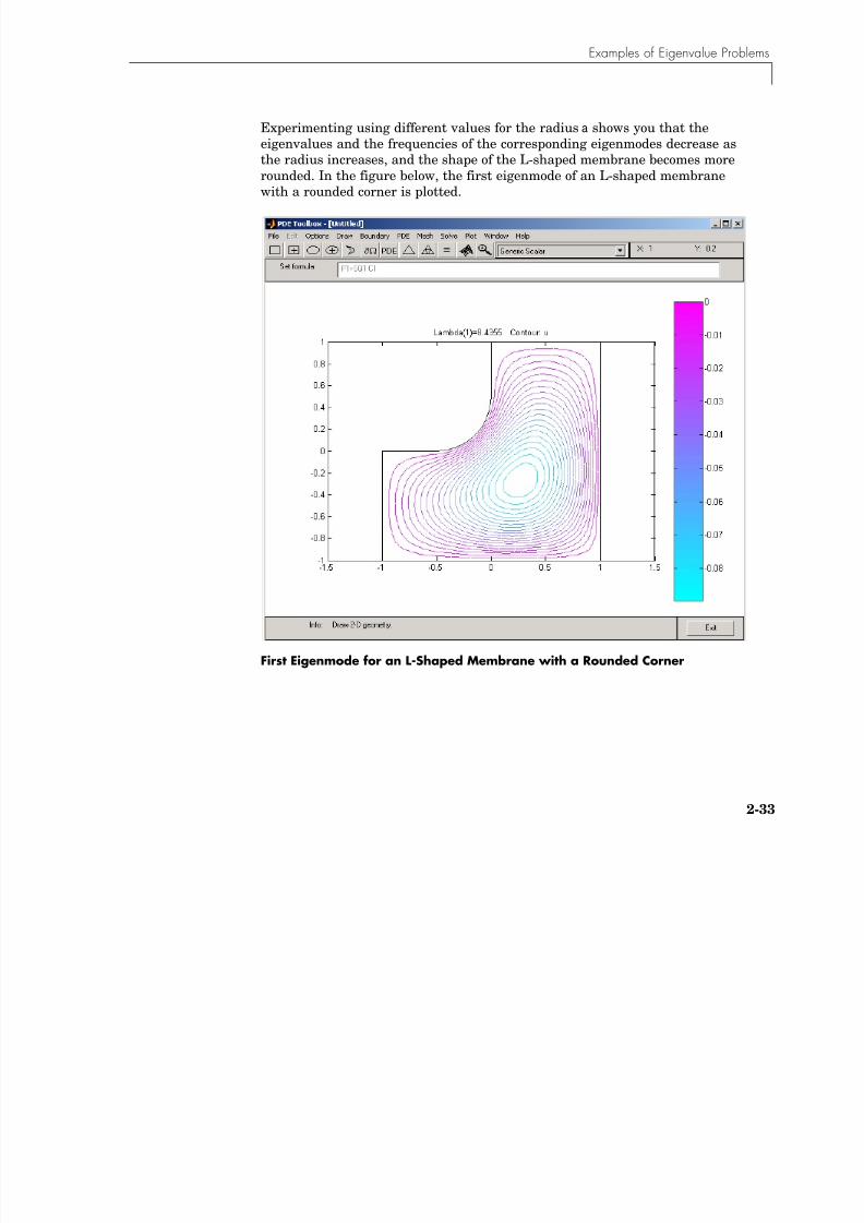
8/21/2019 matlab pde solving.pdf
http://slidepdf.com/reader/full/matlab-pde-solvingpdf 85/290
2-33
Experimenting using different values for the radius a shows you that the
eigenvalues and the frequencies of the corresponding eigenmodes decrease asthe radius increases, and the shape of the L-shaped membrane becomes morerounded. In the figure below, the first eigenmode of an L-shaped membranewith a rounded corner is plotted.
First Eigenmode for an L-Shaped Membrane with a Rounded Corner
2 Examples
8/21/2019 matlab pde solving.pdf
http://slidepdf.com/reader/full/matlab-pde-solvingpdf 86/290
2-34
Eigenvalues and Eigenmodes of a SquareLet us study the eigenvalues and eigenmodes of a square with an interestingset of boundary conditions. The square has corners in (-1,-1), (-1,1), (1,1), and(1,-1). The boundary conditions are as follows:
•On the left boundary, the Dirichlet condition u = 0
•On the upper and lower boundary, the Neumann condition
•On the right boundary, the generalized Neumann condition
The eigenvalue PDE problem is
–∆u = λu
We are interested in the eigenvalues smaller than 10 and the correspondingeigenmodes, so the search range is [ Inf 10]. The sign in the generalizedNeumann condition is such that there are negative eigenvalues.
Using the Graphical User InterfaceUsing the pdetool GUI in the Generic Scalar mode, draw the square using theRectangle/square option from the Draw menu or the button with the
rectangle icon. Then define the boundary conditions by clicking the buttonand then double-click the boundaries to define the boundary conditions. On theright side boundary, you have the generalized Neumann conditions, and youenter them as constants: g = 0 and q = –3/4.
Initialize the mesh and refine it once by clicking the ∆ and refine buttons or byselecting the corresponding options from the Mesh menu.
Also, define the eigenvalue PDE problem by opening the PDE Specification
dialog box and selecting the Eigenmodes option. The general eigenvalue PDEis described by
∂u
∂n
------ 0=
∂u
∂n------
34---u – 0=
Ω∂
∇ – c∇u( )⋅ au+ λdu=
Examples of Eigenvalue Problems
8/21/2019 matlab pde solving.pdf
http://slidepdf.com/reader/full/matlab-pde-solvingpdf 87/290
2-35
so for this problem you use the default values c = 1, a = 0, and d = 1. Also, in
the Solve Parameters dialog box, enter the eigenvalue range as the MATLAB vector [ Inf 10].
Finally, click the = button to compute the solution. By default, the firsteigenfunction is plotted. You can plot the other eigenfunctions by selecting thecorresponding eigenvalue from a pop-up menu in the Plot Selection dialog box.The pop-up menu contains all the eigenvalues found in the specified range. Youcan also export the eigenfunctions and eigenvalues to the MATLAB mainworkspace by using the Export Solution . . . option from the Solve menu.
Using Command-Line FunctionsThe geometry description file and boundary condition file for this problem arecalled squareg.m and squareb2.m, respectively. Use the following sequence ofcommands to find the eigenvalues in the specified range and the correspondingeigenfunctions:
[p,e,t]=initmesh('squareg');
[p,e,t]=refinemesh('squareg',p,e,t);
The eigenvalue PDE coefficients c, a, and d for this problem are c = 1, a = 0, andd = 1. You can enter the eigenvalue range r as the MATLAB vector [ Inf 10].pdeeig returns two output arguments, the eigenvalues as an array l and amatrix v of corresponding eigenfunctions:
[v,l]=pdeeig('squareb2',p,e,t,1,0,1,[ Inf 10]);
To plot the fourth eigenfunction as a surface plot, typepdesurf(p,t,v(:,4))
This problem is separable, i.e.,
The functions f and g are eigenfunctions in the x and y directions, respectively.In the x direction, the first eigenmode is a slowly increasing exponential
function. The higher modes include sinusoids. In the y direction, the firsteigenmode is a straight line (constant), the second is half a cosine, the third isa full cosine, the fourth is one and a half full cosines, etc. These eigenmodes inthe y direction are associated with the eigenvalues:
u x y,( ) f x( ) g y( )=
2 Examples
8/21/2019 matlab pde solving.pdf
http://slidepdf.com/reader/full/matlab-pde-solvingpdf 88/290
2-36
There are five eigenvalues smaller than 10 for this problem, and the first oneis even negative (-0.4145). It is possible to trace the eigenvalues above in theeigenvalues of the solution. Looking at a plot of the first eigenmode, you can seethat it is made up of the first eigenmodes in the x and y directions. The secondeigenmode is made up of the first eigenmode in the x direction and the secondeigenmode in the y direction.
Look at the difference between the first and the second eigenvalue:
l(2) l(1)
ans =
2.4740
pi*pi/4
ans =
2.4674
Likewise, the fifth eigenmode is made up of the first eigenmode in the x
direction and the third eigenmode in the y direction. As expected, l(5) l(1) isapproximately equal to π2. You can explore higher modes by increasing thesearch range to include eigenvalues greater than 10.
0 π
2
4------ 4π
2
4--------- 9π
2
4--------- …, , , ,
Application Modes
8/21/2019 matlab pde solving.pdf
http://slidepdf.com/reader/full/matlab-pde-solvingpdf 89/290
2-37
Application Modes
In this section we describe the application modes of the pdetool graphical userinterface (GUI). Examples are given for a variety of applications to differentengineering problems.
The Application Modes and the GUIThe PDE Toolbox can be applied to a great number of problems in engineering
and science. To help you in using the pdetool GUI for some important andcommon applications, eight different application modes are available inaddition to the generic scalar and system modes.
The available application modes are
•Generic scalar (the default mode)
•Generic system
• “Structural Mechanics — Plane Stress” on page 2-38
• “Structural Mechanics — Plane Strain” on page 2-44
• “Electrostatics” on page 2-44
• “Magnetostatics” on page 2-47
• “AC Power Electromagnetics” on page 2-53
• “Conductive Media DC” on page 2-59
• “Heat Transfer” on page 2-62
• “Diffusion” on page 2-65
Note From the GUI, the system PDEs are restricted to problems with vector valued u of dimension two. Using command-line functions, there is no formalrestriction on the dimension of u.
The application mode can be selected directly from the pop-up menu in theupper right part of the GUI or by selecting an application from the Application submenu in the Options menu. Note that changing the application resets allPDE coefficients and boundary conditions to the default values for that specificapplication mode.
2 Examples
8/21/2019 matlab pde solving.pdf
http://slidepdf.com/reader/full/matlab-pde-solvingpdf 90/290
2-38
When using an application mode, the generic PDE coefficients are replaced by
application-specific parameters such as Young’ s modulus for problems instructural mechanics. The application-specific parameters are entered byselecting Parameters . . . from the PDE menu or by clicking the PDE button. You can also access the PDE parameters by double-clicking a subdomain, if youare in the PDE mode. That way it is possible to define PDE parameters forproblems with regions of different material properties. The Boundary
condition dialog box is also altered so that the Description column reflects thephysical meaning of the different boundary condition coefficients. Finally, the
Plot Selection dialog box allows you to visualize the relevant physical variablesfor the selected application.
Note In the User entry options in the Plot Selection dialog box, the solutionand its derivatives are always referred to as u, ux, and uy (v, vx, and vy for thesystem cases) even if the application mode is nongeneric and the solution ofthe application-specific PDE normally is named, e.g., V or T.
In the remaining part of this section, we explain each of the application modesin more detail and give examples of how to solve application specific problemsusing the PDE Toolbox.
Structural Mechanics — Plane StressIn structural mechanics, the equations relating stress and strain arise from the
balance of forces in the material medium. Plane stress is a condition thatprevails in a flat plate in the xy plane, loaded only in its own plane and without z-direction restraint.
The stress-strain relation can then be written, assuming isotropic andisothermal conditions
σ x
σ y
τ xy# $% &% &% &% &' (
E1 ν
2 –
---------------1 ν 0 ν 1 00 0 1 ν – ( ) 2 ⁄ # $
% &% &% &
' ( ε x
ε y
γ xy# $% &% &% &% &' (
=
Application Modes
8/21/2019 matlab pde solving.pdf
http://slidepdf.com/reader/full/matlab-pde-solvingpdf 91/290
2-39
where σ x and σ y are the stresses in the x and y directions, and τ xy is the shear
stress. The material properties are expressed as a combination of E, the elasticmodulus or Young’s modulus, and ν, Poisson’ s ratio.
The deformation of the material is described by the displacements in the x and
y directions, u and v, from which the strains are defined as
The balance of force equations are
where K x and K y are volume forces (body forces).
Combining the relations above, we arrive at the displacement equations, whichcan be written
–∇ ⋅ (c ⊗∇u) = k
where c is a rank four tensor, which can be written as four 2-by-2 matricesc11, c12, c21, and c22:
where G, the shear modulus, is defined by
ε x∂u
∂ x------ ε y,
∂v
∂ y------ γ xy,
∂u
∂ y------= = =
∂v
∂ x------+
∂σ x
∂ x--------- –
∂τ xy
∂ y----------- – K x=
∂τ xy
∂ x----------- –
∂σ y
∂ y--------- – K y=
c112G µ+ 0
0 G# $% &
' (=
c120 µ
G 0# $% &' (
=
c210 G
µ 0# $% &' (
=
c22G 00 2G µ+# $
% &' (
=
2 Examples
8/21/2019 matlab pde solving.pdf
http://slidepdf.com/reader/full/matlab-pde-solvingpdf 92/290
2-40
and µ in turn is defined by
are volume forces.
This is an elliptic PDE of system type (u is two-dimensional), but you need onlyto select the application mode Structural Mechanics, Plane Stress and thenenter the material-dependent parameters E and ν and the volume forces k intothe PDE Specification dialog box.
In this mode, you can also solve the eigenvalue problem, which is described by–∇ ⋅ (c ⊗∇u) = λdu
d =
ρ, the density, can also be entered using the PDE Specification dialog box.
In the Plot Selection dialog box, the x- and y-displacements, u and v, and theabsolute value of the displacement vector (u,v) can be visualized using color,contour lines, or z-height, and the displacement vector field (u,v) can be plottedusing arrows or a deformed mesh. In addition, for visualization using color,contour lines, or height, you can choose from 15 scalar tensor expressions:
•
•
•
•
• exx, the x-direction strain (ε x)
• eyy, the y-direction strain (ε y)
• exy, the shear strain (γ xy)
G E
2 1 ν+( )---------------------=
µ 2Gv
1 ν – ------------=
k K x
K y# $% &% &' (
=
ρ 00 ρ# $
% &' (
ux ∂u
∂ x------=
uy ∂u
∂ y------=
vx ∂v∂ x------=
vy ∂v
∂ y------=
Application Modes
8/21/2019 matlab pde solving.pdf
http://slidepdf.com/reader/full/matlab-pde-solvingpdf 93/290
2-41
• sxx, the x-direction stress (σ x)
• syy, the y-direction stress (σ y)• sxy, the shear stress (τ xy)
• e1, the first principal strain (ε1)
• e2, the second principal strain (ε 2)
• s1, the first principal stress (σ1)
• s2, the second principal stress (σ 2)
•von Mises, the von Mises effective stress
For a more detailed discussion on the theory of stress-strain relations andapplications of FEM to problems in structural mechanics, see [1].
Example
Consider a steel plate that is clamped along a right-angle inset at the lower leftcorner, and pulled along a rounded cut at the upper right corner. All other sidesare free.
The steel plate has the following properties: Dimension: 1-by-1 meters;thickness 1mm; inset is 1/3-by-1/3 meters. The rounded cut runs from (2/3, 1)to (1, 2/3). Young’ s modulus: 196 ⋅ 103 (MN/m2), Poisson’ s ratio: 0.31.
The curved boundary is subjected to an outward normal load of 500 N/m. Weneed to specify a surface traction; we therefore divide by the thickness 1 mm,thus the surface tractions should be set to 0.5 MN/m2. We will use the force unitMN in this example.
We want to compute a number of interesting quantities, such as the x- and y-direction strains and stresses, the shear stress, and the von Mises effectivestress.
Using the Graphical User InterfaceUsing the pdetool GUI, the first thing to do is to select the application mode.For this problem, use Structural Mechanics, Plane Stress.
The CSG model can be made very quickly by drawing a polygon with corners in
x=[0 2/3 1 1 1/3 1/3 0] and y=[1 1 2/3 0 0 1/3 1/3] and a circle withcenter in x=2/3, y=2/3 and radius 1/3.
σ12
σ22
σ1σ2 – +( )
2 Examples
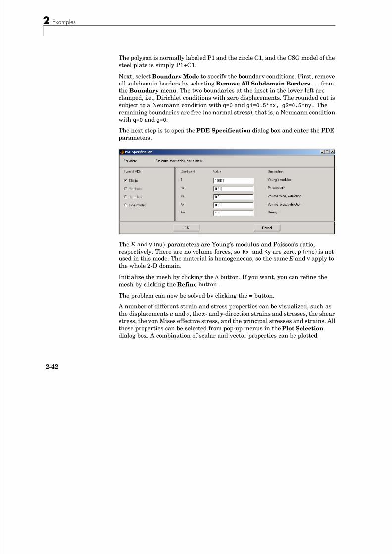
8/21/2019 matlab pde solving.pdf
http://slidepdf.com/reader/full/matlab-pde-solvingpdf 94/290
2-42
The polygon is normally labeled P1 and the circle C1, and the CSG model of the
steel plate is simply P1+C1.Next, select Boundary Mode to specify the boundary conditions. First, removeall subdomain borders by selecting Remove All Subdomain Borders . . . fromthe Boundary menu. The two boundaries at the inset in the lower left areclamped, i.e., Dirichlet conditions with zero displacements. The rounded cut issubject to a Neumann condition with q=0 and g1=0.5*nx, g2=0.5*ny. Theremaining boundaries are free (no normal stress), that is, a Neumann conditionwith q=0 and g=0.
The next step is to open the PDE Specification dialog box and enter the PDEparameters.
The E and ν (nu) parameters are Young’ s modulus and Poisson’ s ratio,respectively. There are no volume forces, so Kx and Ky are zero. ρ (rho) is notused in this mode. The material is homogeneous, so the same E and ν apply tothe whole 2-D domain.
Initialize the mesh by clicking the ∆ button. If you want, you can refine themesh by clicking the Refine button.
The problem can now be solved by clicking the = button.
A number of different strain and stress properties can be visualized, such asthe displacements u and v, the x- and y-direction strains and stresses, the shearstress, the von Mises effective stress, and the principal stresses and strains. Allthese properties can be selected from pop-up menus in the Plot Selection dialog box. A combination of scalar and vector properties can be plotted
Application Modes
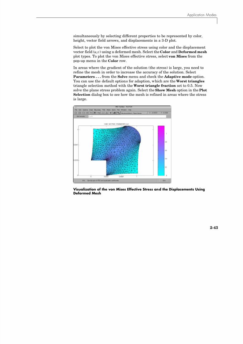
8/21/2019 matlab pde solving.pdf
http://slidepdf.com/reader/full/matlab-pde-solvingpdf 95/290
2-43
simultaneously by selecting different properties to be represented by color,
height, vector field arrows, and displacements in a 3-D plot.Select to plot the von Mises effective stress using color and the displacement vector field (u,v) using a deformed mesh. Select the Color and Deformed mesh plot types. To plot the von Mises effective stress, select von Mises from thepop-up menu in the Color row.
In areas where the gradient of the solution (the stress) is large, you need torefine the mesh in order to increase the accuracy of the solution. Select
Parameters . . . from the Solve menu and check the Adaptive mode option. You can use the default options for adaption, which are the Worst triangles triangle selection method with the Worst triangle fraction set to 0.5. Nowsolve the plane stress problem again. Select the Show Mesh option in the Plot
Selection dialog box to see how the mesh is refined in areas where the stressis large.
Visualization of the von Mises Effective Stress and the Displacements UsingDeformed Mesh
2 Examples
8/21/2019 matlab pde solving.pdf
http://slidepdf.com/reader/full/matlab-pde-solvingpdf 96/290
2-44
Structural Mechanics — Plane Strain A deformation state where there are no displacements in the z-direction, andthe displacements in the x- and y-directions are functions of x and y but not zis called plane strain. You can solve plane strain problems with the PDEToolbox by selecting the application mode Structural Mechanics, Plane
Strain. The stress-strain relation is only slightly different from the planestress case, and the same set of material parameters is used. The applicationinterfaces are identical for the two structural mechanics modes.
The places where the plane strain equations differ from the plane stressequations are
•The µ parameter in the c tensor is defined as
•The von Mises effective stress is computed as
Plane strain problems are less common than plane stress problems. Anexample is a slice of an underground tunnel that lies along the z-axis. Itdeforms in essentially plane strain conditions.
Electrostatics
Applications involving electrostatics include high voltage apparatus, electronicdevices, and capacitors. The “statics” implies that the time rate of change isslow, and that wavelengths are very large compared to the size of the domainof interest. In electrostatics, the electrostatic scalar potential V is related to theelectric field E by E = –∇V and, using one of Maxwell’s equations, ∇ ⋅ D = ρ andthe relationship D = εE, we arrive at the Poisson equation
where ε is the coefficient of dielectricity and ρ is the space charge density.
µ 2G ν
1 2 ν – ----------------=
σ12
σ22
+( ) ν2
ν – 1+( ) σ1σ2 2 ν2 2 ν – 1 – ( ) –
∇ – ε∇V ( )⋅ ρ=
Application Modes
8/21/2019 matlab pde solving.pdf
http://slidepdf.com/reader/full/matlab-pde-solvingpdf 97/290
2-45
Note ε should really be written as εε0, where ε0 is the coefficient ofdielectricity or permittivity of vacuum (8.854 ⋅ 10-12 farad/meter) and ε is therelative coefficient of dielectricity that varies among different dielectrics(1.00059 in air, 2.24 in transformer oil, etc.).
Using the PDE Toolbox application mode Electrostatics, you can solveelectrostatic problems modeled by the equation above.
The PDE Specification dialog box contains entries for ε and ρ.
The boundary conditions for electrostatic problems can be of Dirichlet orNeumann type. For Dirichlet conditions, the electrostatic potential V isspecified on the boundary. For Neumann conditions, the surface charge
n ⋅ (ε∇V ) is specified on the boundary.
For visualization of the solution to an electrostatic problem, the plot selections
include the electrostatic potential V , the electric field E, and the electricdisplacement field D.
For a more in-depth discussion of problems in electrostatics, see [2].
ExampleLet us consider the problem of determining the electrostatic potential in anair-filled quadratic “frame,” bounded by a square with side length of 0.2 in thecenter and by outer limits with side length of 0.5. At the inner boundary, theelectrostatic potential is 1000V. At the outer boundary, the electrostaticpotential is 0V. There is no charge in the domain. This leads to the problem ofsolving the Laplace equation
∆V = 0
with the Dirichlet boundary conditions V = 1000 at the inner boundary,and V = 0 at the outer boundary.
Using the Graphical User Interface After selecting the application mode Electrostatics, the 2-D area is most easilydrawn by first drawing a square with sides of length 0.2 (use the Snap optionand adjust the grid spacing if necessary). Then draw another square with sidesof length 0.5 using the same center position. The 2-D domain is then simply
2 Examples
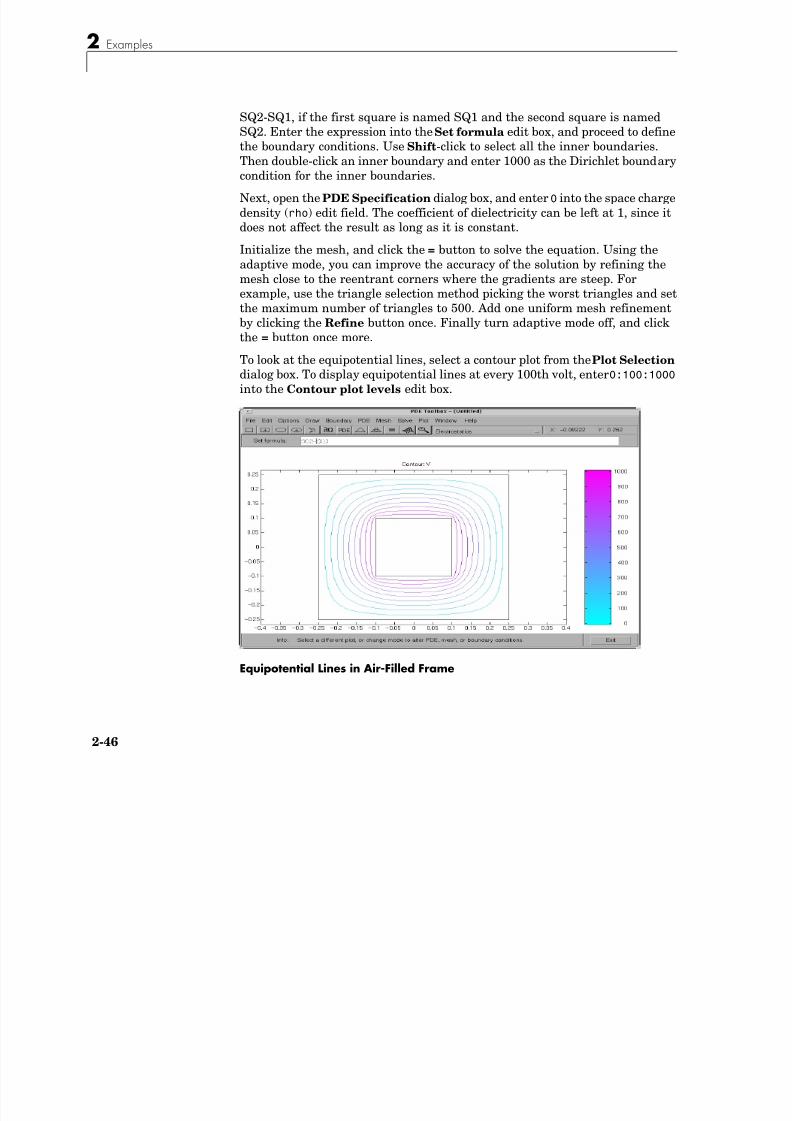
8/21/2019 matlab pde solving.pdf
http://slidepdf.com/reader/full/matlab-pde-solvingpdf 98/290
2-46
SQ2-SQ1, if the first square is named SQ1 and the second square is named
SQ2. Enter the expression into the Set formula edit box, and proceed to definethe boundary conditions. Use Shift-click to select all the inner boundaries.Then double-click an inner boundary and enter 1000 as the Dirichlet boundarycondition for the inner boundaries.
Next, open the PDE Specification dialog box, and enter 0 into the space chargedensity (rho) edit field. The coefficient of dielectricity can be left at 1, since itdoes not affect the result as long as it is constant.
Initialize the mesh, and click the = button to solve the equation. Using theadaptive mode, you can improve the accuracy of the solution by refining themesh close to the reentrant corners where the gradients are steep. Forexample, use the triangle selection method picking the worst triangles and setthe maximum number of triangles to 500. Add one uniform mesh refinementby clicking the Refine button once. Finally turn adaptive mode off, and clickthe = button once more.
To look at the equipotential lines, select a contour plot from the Plot Selection
dialog box. To display equipotential lines at every 100th volt, enter 0:100:1000 into the Contour plot levels edit box.
Equipotential Lines in Air-Filled Frame
Application Modes
8/21/2019 matlab pde solving.pdf
http://slidepdf.com/reader/full/matlab-pde-solvingpdf 99/290
2-47
MagnetostaticsMagnets, electric motors, and transformers are areas where problemsinvolving magnetostatics can be found. The “statics” implies that the time rateof change is slow, so we start with Maxwell’s equations for steady cases,
∇ × H = J
∇ ⋅ B = 0
and the relationship
B = µH
where B is the magnetic flux density, H is the magnetic field intensity, J is thecurrent density, and µ is the material’s magnetic permeability.
Since ∇ ⋅ B = 0, there exists a magnetic vector potential A such that
B = ∇ × A
and
The plane case assumes that the current flows are parallel to the z-axis, so onlythe z component of A is present,
A = (0,0, A),J = (0,0, J )
and the equation above can be simplified to the scalar elliptic PDE
where J = J ( x,y).
For the 2-D case, we can compute the magnetic flux density B as
and the magnetic field H, in turn, is given by
1µ---∇ A×# $
' (∇× J =
∇ – 1µ---∇ A# $
' (⋅ J =
B ∂ A∂ y------- ∂ A
∂ x------- – 0, ,# $' (=
H 1µ--- B=
2 Examples

8/21/2019 matlab pde solving.pdf
http://slidepdf.com/reader/full/matlab-pde-solvingpdf 100/290
2-48
The interface condition across subdomain borders between regions of different
material properties is that H × n be continuous. This implies the continuity of
and does not require special treatment since we are using the variationalformulation of the PDE problem.
In ferromagnetic materials, µ is usually dependent on the field strength
|B| = |∇ A|, so the nonlinear solver is needed.The Dirichlet boundary condition specifies the value of the magnetostaticpotential A on the boundary. The Neumann condition specifies the value of thenormal component of
on the boundary. This is equivalent to specifying the tangential value of themagnetic field H on the boundary.
Visualization of the magnetostatic potential A, the magnetic field H, and themagnetic flux density B is available. B and H can be plotted as vector fields.
See [2] for a more detailed discussion on Maxwell’s equations andmagnetostatics.
Example As an example of a problem in magnetostatics, consider determining the staticmagnetic field due to the stator windings in a two-pole electric motor. Themotor is considered to be long, and when end effects are neglected, a 2-Dcomputational model suffices.
The domain consists of three regions:
•Two ferromagnetic pieces, the stator and the rotor
•The air gap between the stator and the rotor•The armature coil carrying the DC current
The magnetic permeability µ is 1 in the air and in the coil. In the stator and therotor, µ is defined by
1µ---
∂ A
∂n-------
n1µ--- A∇# $
' (
Application Modes

8/21/2019 matlab pde solving.pdf
http://slidepdf.com/reader/full/matlab-pde-solvingpdf 101/290
2-49
µmax = 5000, µmin = 200, and c = 0.05 are values that could representtransformer steel.
The current density J is 0 everywhere except in the coil, where it is 1.
The geometry of the problem makes the magnetic vector potential A symmetricwith respect to y and anti-symmetric with respect to x, so you can limit the
domain to x ≥ 0, y≥0 with the Neumann boundary condition
on the x-axis and the Dirichlet boundary condition A = 0 on the y-axis. The fieldoutside the motor is neglected leading to the Dirichlet boundary condition A = 0 on the exterior boundary.
Using the Graphical User InterfaceThe geometry is complex, involving five circular arcs and two rectangles. Usingthe pdetool GUI, set the x-axis limits to [-1.5 1.5] and the y-axis limits to[ 1 1]. Set the application mode to Magnetostatics, and use a grid spacing of0.1. The model is a union of circles and rectangles; the reduction to the firstquadrant is achieved by intersection with a square. Using the “snap-to-grid”feature, you can draw the geometry using the mouse, or you can draw it by
entering the following commands:pdecirc(0,0,1,'C1')
pdecirc(0,0,0.8,'C2')
pdecirc(0,0,0.6,'C3')
pdecirc(0,0,0.5,'C4')
pdecirc(0,0,0.4,'C5')
pderect([-0.2 0.2 0.2 0.9],'R1')
pderect([-0.1 0.1 0.2 0.9],'R2')
pderect([0 1 0 1],'SQ1')
You should get a CSG model similar to the one in the plot below.
µ
µmax
1 c ∇ A( ) 2+---------------------------------- µmi n+=
n1µ--- A∇# $
' (⋅ 0=
2 Examples
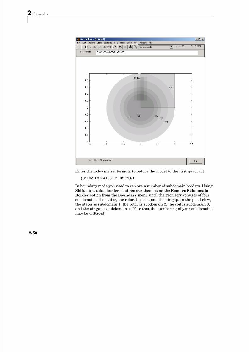
8/21/2019 matlab pde solving.pdf
http://slidepdf.com/reader/full/matlab-pde-solvingpdf 102/290
2-50
Enter the following set formula to reduce the model to the first quadrant:
(C1+C2+C3+C4+C5+R1+R2)*SQ1
In boundary mode you need to remove a number of subdomain borders. Using
Shift-click, select borders and remove them using the Remove SubdomainBorder option from the Boundary menu until the geometry consists of foursubdomains: the stator, the rotor, the coil, and the air gap. In the plot below,the stator is subdomain 1, the rotor is subdomain 2, the coil is subdomain 3,and the air gap is subdomain 4. Note that the numbering of your subdomainsmay be different.
Application Modes
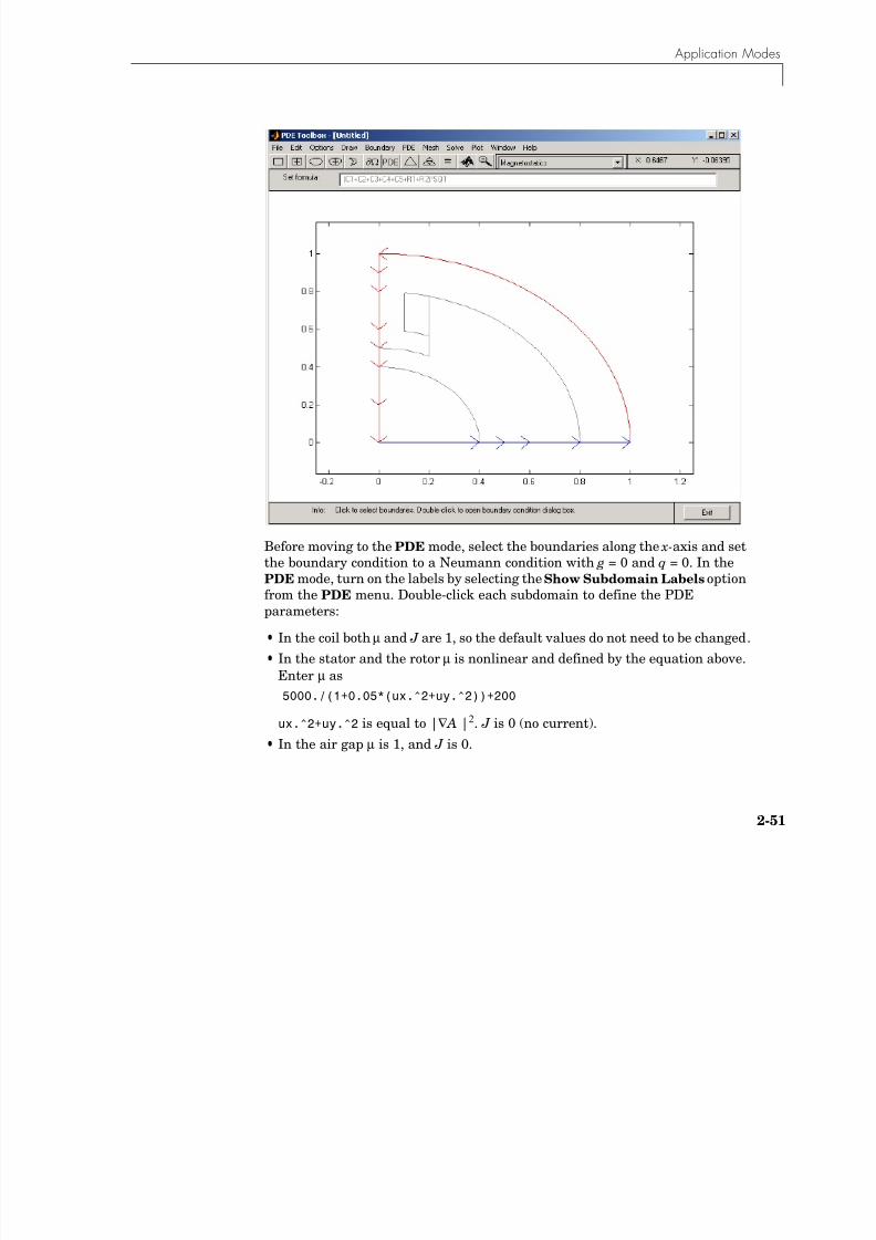
8/21/2019 matlab pde solving.pdf
http://slidepdf.com/reader/full/matlab-pde-solvingpdf 103/290
2-51
Before moving to the PDE mode, select the boundaries along the x-axis and setthe boundary condition to a Neumann condition with g = 0 and q = 0. In thePDE mode, turn on the labels by selecting the Show Subdomain Labels optionfrom the PDE menu. Double-click each subdomain to define the PDEparameters:
• In the coil both µ and J are 1, so the default values do not need to be changed.
• In the stator and the rotor µ is nonlinear and defined by the equation above.
Enter µ as5000./(1+0.05*(ux.^2+uy.^2))+200
ux.^2+uy.^2 is equal to |∇ A |2. J is 0 (no current).
• In the air gap µ is 1, and J is 0.
2 Examples

8/21/2019 matlab pde solving.pdf
http://slidepdf.com/reader/full/matlab-pde-solvingpdf 104/290
2-52
Initialize the mesh, and continue by opening the Solve Parameters dialog box
by selecting Parameters from the Solve menu. Since this is a nonlinearproblem, the nonlinear solver must be invoked by checking the Use nonlinear
solver. If you want, you can adjust the tolerance parameter. The adaptivesolver can be used together with the nonlinear solver. Solve the PDE and plotthe magnetic flux density B using arrows and the equipotential lines of themagnetostatic potential A using a contour plot. The plot clearly shows, asexpected, that the magnetic flux is parallel to the equipotential lines of themagnetostatic potential.
Equipotential Lines and Magnetic Flux in Two-Pole Motor
Application Modes
8/21/2019 matlab pde solving.pdf
http://slidepdf.com/reader/full/matlab-pde-solvingpdf 105/290
2-53
AC Power Electromagnetics
AC power electromagnetics problems are found when studying motors,transformers and conductors carrying alternating currents.
Let us start by considering a homogeneous dielectric, with coefficient ofdielectricity ε and magnetic permeability µ, with no charges at any point. Thefields must satisfy a special set of the general Maxwell’s equations; see [2]:
In the absence of current, we can eliminate H from the first set and E from thesecond set and see that both fields satisfy wave equations with wave speed
We move on to studying a charge-free homogeneous dielectric, with coefficientof dielectrics ε, magnetic permeability µ, and conductivity σ. The currentdensity then is
J = σE
and the waves are damped by the Ohmic resistance,
and similarly for H.
The case of time harmonic fields is treated by using the complex form, replacing
E by Ec e jωt
The plane case of this PDE Toolbox mode has Ec = (0,0, Ec) and J = (0,0, Je jωt),and the magnetic field
∇ E× µ – ∂H
∂t--------=
∇ H× ε∂E
∂t------- J+=
εµ
E∆ εµ ∂2E
∂t2
---------- – 0 H∆, εµ ∂2H
∂t2
----------- 0= – =
E∆ µσ∂E
∂t------- – εµ
∂2E
∂t2
---------- – 0=
2 Examples
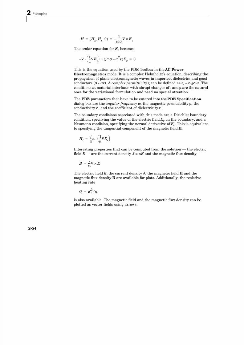
8/21/2019 matlab pde solving.pdf
http://slidepdf.com/reader/full/matlab-pde-solvingpdf 106/290
2-54
The scalar equation for Ec becomes
This is the equation used by the PDE Toolbox in the AC Power
Electromagnetics mode. It is a complex Helmholtz’s equation, describing the
propagation of plane electromagnetic waves in imperfect dielectrics and goodconductors (σ » ωε). A complex permittivity εccan be defined as εc = ε− jσ/ω. Theconditions at material interfaces with abrupt changes of ε and µ are the naturalones for the variational formulation and need no special attention.
The PDE parameters that have to be entered into the PDE Specification dialog box are the angular frequency ω, the magnetic permeability µ, theconductivity σ, and the coefficient of dielectricity ε.
The boundary conditions associated with this mode are a Dirichlet boundarycondition, specifying the value of the electric field Ec on the boundary, and aNeumann condition, specifying the normal derivative of Ec. This is equivalentto specifying the tangential component of the magnetic field H:
Interesting properties that can be computed from the solution — the electricfield E — are the current density J = σ E and the magnetic flux density
The electric field E, the current density J , the magnetic field H and themagnetic flux density B are available for plots. Additionally, the resistiveheating rate
is also available. The magnetic field and the magnetic flux density can beplotted as vector fields using arrows.
H H x
H y
0, ,( )1
jµσ---------∇ E
c× – = =
∇ – 1µ---∇ Ec# $
' (⋅ jωσ ω2
ε – ( ) Ec+ 0=
H t j
ω----n
1µ--- Ec∇# $
' (⋅=
B j
ω----∇ E×=
Q Ec2
σ ⁄ =
Application Modes

8/21/2019 matlab pde solving.pdf
http://slidepdf.com/reader/full/matlab-pde-solvingpdf 107/290
2-55
Example
The example demonstrates the skin effect when AC current is carried by a wirewith circular cross section. The conductivity of copper is 57 ⋅ 106, and thepermeability is 1, i.e., µ = 4π10-7. At the line frequency (50 Hz) the ω2ε-term isnegligible.
Due to the induction, the current density in the interior of the conductor issmaller than at the outer surface where it is set to J S = 1, a Dirichlet conditionfor the electric field, Ec = 1/ σ. For this case an analytical solution is available,
where
R is the radius of the wire, r is the distance from the centerline, and J 0( x) is the
first Bessel function of zeroth order.
Using the Graphical User InterfaceStart the pdetool GUI and select the application mode AC Power
Electromagnetics. Draw a circle with radius 0.1 to represent a cross section ofthe conductor, and proceed to the boundary mode to define the boundarycondition. Use the Select All option to select all boundaries and enter 1/57E6
into the r edit field in the Boundary Condition dialog box to define the
Dirichlet boundary condition ( E = J/σ).Open the PDE Specification dialog box and enter the PDE parameters. Theangular frequency ω = 2 ⋅ π ⋅ 50.
J J S J 0 kr( )
J 0 kR( )-------------------=
k jωµ σ=
2 Examples
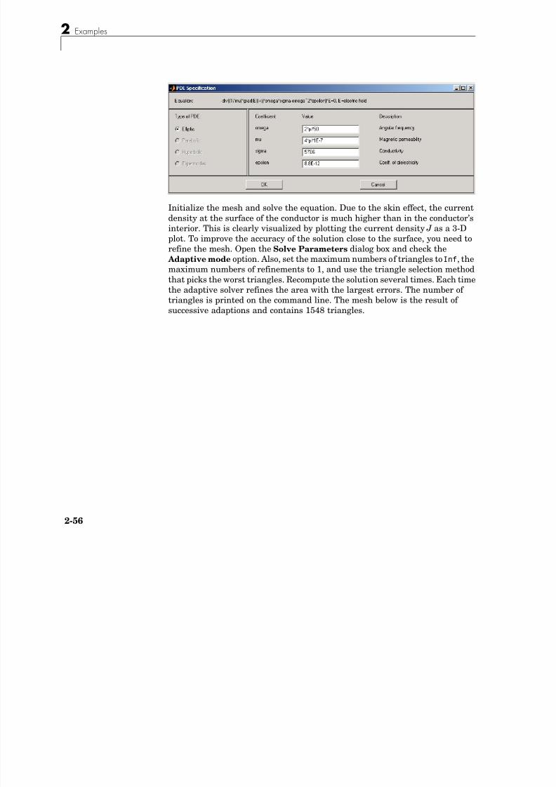
8/21/2019 matlab pde solving.pdf
http://slidepdf.com/reader/full/matlab-pde-solvingpdf 108/290
2-56
Initialize the mesh and solve the equation. Due to the skin effect, the currentdensity at the surface of the conductor is much higher than in the conductor’sinterior. This is clearly visualized by plotting the current density J as a 3-Dplot. To improve the accuracy of the solution close to the surface, you need torefine the mesh. Open the Solve Parameters dialog box and check the
Adaptive mode option. Also, set the maximum numbers of triangles to Inf, themaximum numbers of refinements to 1, and use the triangle selection methodthat picks the worst triangles. Recompute the solution several times. Each timethe adaptive solver refines the area with the largest errors. The number oftriangles is printed on the command line. The mesh below is the result ofsuccessive adaptions and contains 1548 triangles.
Application Modes

8/21/2019 matlab pde solving.pdf
http://slidepdf.com/reader/full/matlab-pde-solvingpdf 109/290
2-57
The Adaptively Refined Mesh
The solution of the AC power electromagnetics equation is complex. The plotsshow the real part of the solution (a warning message is issued), but thesolution vector, which can be exported to the main workspace, is the full
complex solution. Also, you can plot various properties of the complex solutionby using the user entry. imag(u) and abs(u) are two examples of valid userentries.
2 Examples
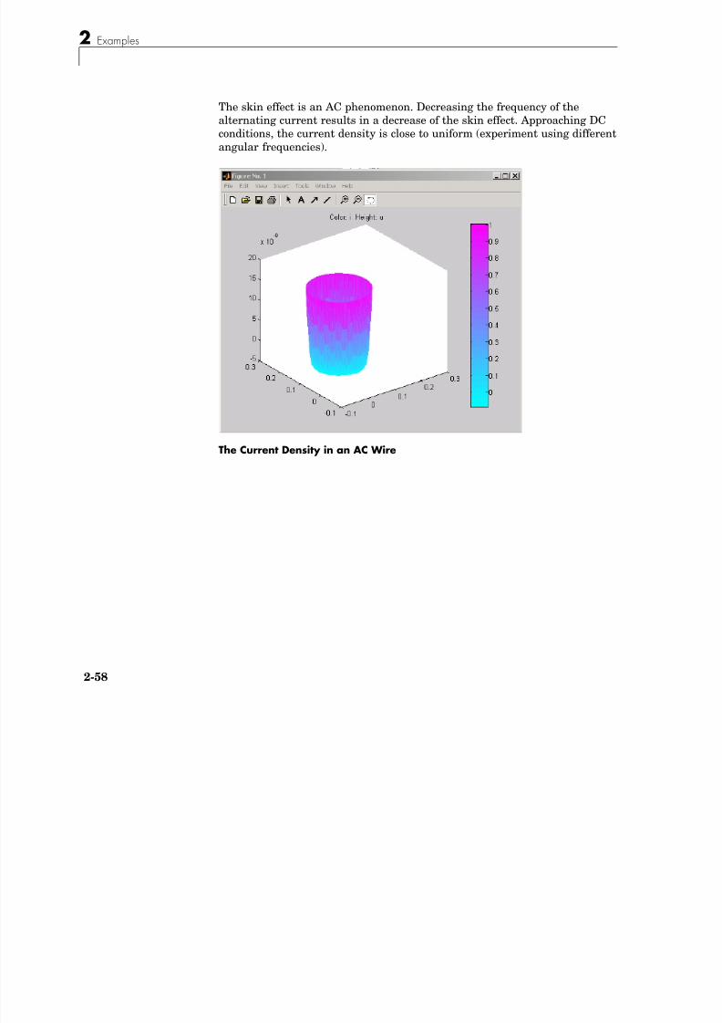
8/21/2019 matlab pde solving.pdf
http://slidepdf.com/reader/full/matlab-pde-solvingpdf 110/290
2-58
The skin effect is an AC phenomenon. Decreasing the frequency of the
alternating current results in a decrease of the skin effect. Approaching DCconditions, the current density is close to uniform (experiment using differentangular frequencies).
The Current Density in an AC Wire
Application Modes
8/21/2019 matlab pde solving.pdf
http://slidepdf.com/reader/full/matlab-pde-solvingpdf 111/290
2-59
Conductive Media DC
For electrolysis and computation of resistances of grounding plates, we have aconductive medium with conductivity σ and a steady current. The currentdensity J is related to the electric field E through J = σE. Combining thecontinuity equation ∇ ⋅ J = Q, where Q is a current source, with the definitionof the electric potential V yields the elliptic Poisson’s equation
–∇ ⋅ (σ∇V ) = Q
The only two PDE parameters are the conductivity σ and the current source Q.
The Dirichlet boundary condition assigns values of the electric potential V tothe boundaries, usually metallic conductors. The Neumann boundary conditionrequires the value of the normal component of the current density (n ⋅ (σ ∇(V)))to be known. It is also possible to specify a generalized Neumann conditiondefined by n ⋅ (σ ∇(V) + qV = g, where q can be interpreted as a film conductance for thin plates.
The electric potential V , the electric field E, and the current density J are all
available for plotting. Interesting quantities to visualize are the current lines(the vector field of J) and the equipotential lines of V . The equipotential linesare orthogonal to the current lines when σ is isotropic.
ExampleTwo circular metallic conductors are placed on a plane, thin conductor like ablotting paper wetted by brine. The equipotentials can be traced by a voltmeterwith a simple probe, and the current lines can be traced by strongly colored
ions, such as permanganate ions.The physical model for this problem consists of the Laplace equation
–∇ ⋅ (σ∇V ) = 0
for the electric potential V and the boundary conditions:
•V = 1 on the left circular conductor
•
V = –1 on the right circular conductor•The natural Neumann boundary condition on the outer boundaries
∂V
∂n------- 0=
2 Examples
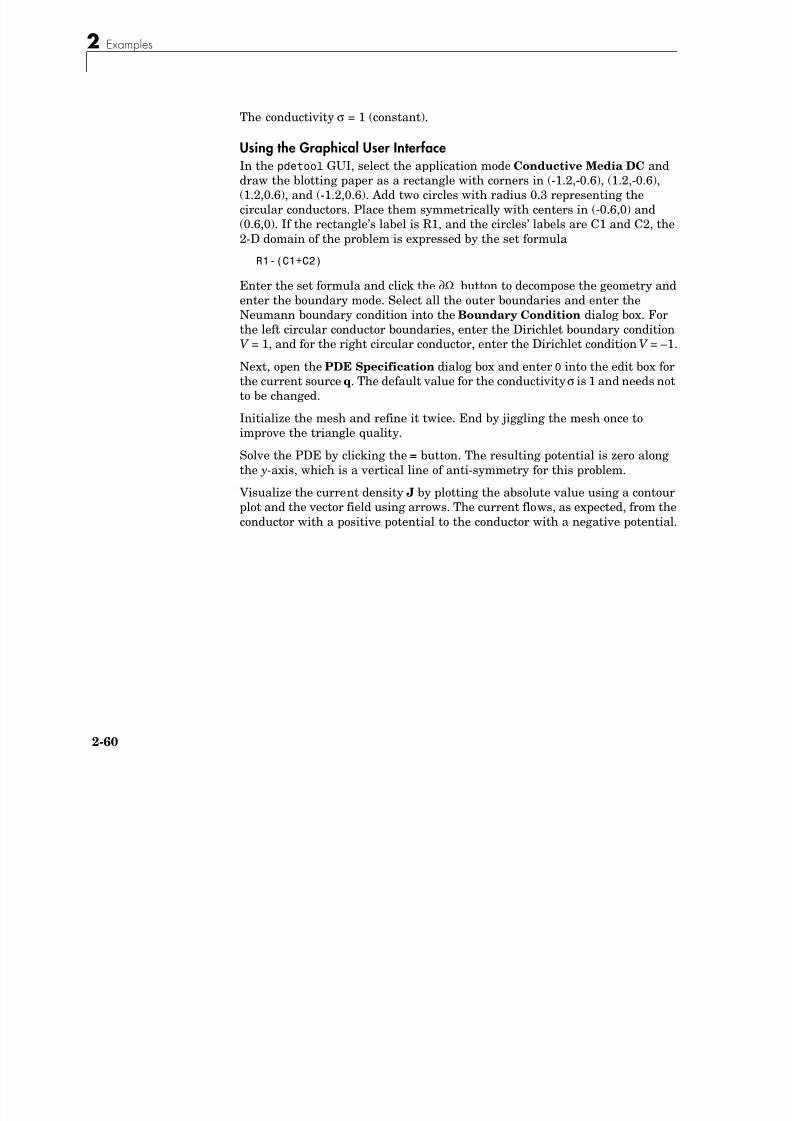
8/21/2019 matlab pde solving.pdf
http://slidepdf.com/reader/full/matlab-pde-solvingpdf 112/290
2-60
The conductivity σ = 1 (constant).
Using the Graphical User InterfaceIn the pdetool GUI, select the application mode Conductive Media DC anddraw the blotting paper as a rectangle with corners in (-1.2,-0.6), (1.2,-0.6),(1.2,0.6), and (-1.2,0.6). Add two circles with radius 0.3 representing thecircular conductors. Place them symmetrically with centers in (-0.6,0) and(0.6,0). If the rectangle’s label is R1, and the circles’ labels are C1 and C2, the2-D domain of the problem is expressed by the set formula
R1-(C1+C2)
Enter the set formula and click the button to decompose the geometry andenter the boundary mode. Select all the outer boundaries and enter theNeumann boundary condition into the Boundary Condition dialog box. Forthe left circular conductor boundaries, enter the Dirichlet boundary conditionV = 1, and for the right circular conductor, enter the Dirichlet condition V = –1.
Next, open thePDE Specification
dialog box and enter0
into the edit box forthe current source q. The default value for the conductivity σ is 1 and needs notto be changed.
Initialize the mesh and refine it twice. End by jiggling the mesh once toimprove the triangle quality.
Solve the PDE by clicking the = button. The resulting potential is zero alongthe y-axis, which is a vertical line of anti-symmetry for this problem.
Visualize the current density J by plotting the absolute value using a contourplot and the vector field using arrows. The current flows, as expected, from theconductor with a positive potential to the conductor with a negative potential.
Ω∂
Application Modes
8/21/2019 matlab pde solving.pdf
http://slidepdf.com/reader/full/matlab-pde-solvingpdf 113/290
2-61
The Current Density Between Two Metallic Conductors
2 Examples
f
8/21/2019 matlab pde solving.pdf
http://slidepdf.com/reader/full/matlab-pde-solvingpdf 114/290
2-62
Heat Transfer
The heat equation is a parabolic PDE:
It describes the heat transfer process for plane and axisymmetric cases, anduses the following parameters:
•Density ρ
•Heat capacity C•Coefficient of heat conduction k
•Heat source Q
•Convective heat transfer coefficient h
•External temperature T ext
The term h ⋅ (T ext – T ) is a model of transversal heat transfer from the
surroundings, and it may be useful for modeling heat transfer in thin coolingplates etc.
For the steady state case, the elliptic version of the heat equation,
is also available.
The boundary conditions can be of Dirichlet type, where the temperature onthe boundary is specified, or of Neumann type where the heat flux, n ⋅ (k∇(T ))is specified. A generalized Neumann boundary condition can also be used. Thegeneralized Neumann boundary condition equation is n ⋅ (k∇(T )) + qT = g,where q is the heat transfer coefficient.
Visualization of the temperature, the temperature gradient, and the heatflux k∇T is available. Plot options include isotherms and heat flux vector fieldplots.
ExampleIn the following example, a heat transfer problem with differing materialparameters is solved.
ρC∂T
∂t------- ∇ – k∇T ( )⋅ Q h+ T ex t T – ( )⋅=
∇ – k∇T ( )⋅ Q h+ T ex t T – ( )⋅=
Application Modes

8/21/2019 matlab pde solving.pdf
http://slidepdf.com/reader/full/matlab-pde-solvingpdf 115/290
2-63
The problem’s 2-D domain consists of a square with an embedded diamond (a
square with 45 degrees rotation). The square region consists of a material withcoefficient of heat conduction of 10 and a density of 2. The diamond-shapedregion contains a uniform heat source of 4, and it has a coefficient of heatconduction of 2 and a density of 1. Both regions have a heat capacity of 0.1.
Using the Graphical User InterfaceStart the pdetool GUI and select the application mode Heat Transfer. In drawmode, set the x- and y-axis limits to [-0.5 3.5] and select the Axis Equal
option from the Options menu. The square region has corners in (0,0), (3,0),(3,3), and (0,3). The diamond-shaped region has corners in (1.5,0.5), (2.5,1.5),(1.5,2.5), and (0.5,1.5).
The temperature is kept at 0 on all the outer boundaries, so you do not have tochange the default boundary conditions. Move on to define the PDE parameters(make sure that the Heat Transfer application mode is selected) in the PDEmode by double-clicking each of the two regions and enter the PDE parameters. You want to solve the parabolic heat equation, so make sure that the Parabolic option is selected. In the square region, enter a density of 2, a heat capacity of0.1, and a coefficient of heat conduction of 10. There is no heat source, so set itto 0. In the diamond-shaped region, enter a density of 1, a heat capacity of 0.1,and a coefficient of heat conduction of 2. Enter 4 in the edit field for the heatsource. The transversal heat transfer term h ⋅ (T ext – T ) is not used, so set h,the convective heat transfer coefficient, to 0.
Since you are solving a dynamic PDE, you have to define an initial value, and
the times at which you want to solve the PDE. Open the Solve Parameters dialog box by selecting Parameters . . . from the Solve menu. The dynamics forthis problem is very fast — the temperature reaches steady state in about 0.1time units. To capture the interesting part of the dynamics, enterlogspace(-2,-1,10) as the vector of times at which to solve the heat equation.logspace(-2,-1,10) gives 10 logarithmically spaced numbers between 0.01and 0.1. Set the initial value of the temperature to 0. If the boundary conditionsand the initial value differ, the problem formulation contains discontinuities.
Solve the PDE. By default, the temperature distribution at the last time isplotted. The best way to visualize the dynamic behavior of the temperature isto animate the solution. When animating, turn on the Height (3-D plot) optionto animate a 3-D plot. Also, select the Plot in x-y grid option. Using arectangular grid instead of a triangular grid speeds up the animation processsignificantly.
2 Examples
O h i i i li i d b l i i h l li i
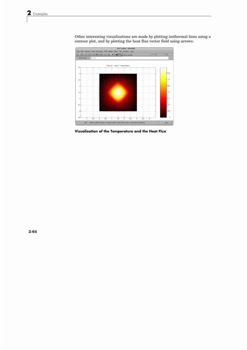
8/21/2019 matlab pde solving.pdf
http://slidepdf.com/reader/full/matlab-pde-solvingpdf 116/290
2-64
Other interesting visualizations are made by plotting isothermal lines using a
contour plot, and by plotting the heat flux vector field using arrows.
Visualization of the Temperature and the Heat Flux
Application Modes
Diff i
8/21/2019 matlab pde solving.pdf
http://slidepdf.com/reader/full/matlab-pde-solvingpdf 117/290
2-65
Diffusion
Since heat transfer is a diffusion process, the generic diffusion equation has thesame structure as the heat equation:
where c is the concentration, D is the diffusion coefficient and Q is a volumesource. The diffusion process may be anisotropic, in which case D is a 2-by-2matrix.
The boundary conditions can be of Dirichlet type, where the concentration onthe boundary is specified, or of Neumann type, where the flux n ⋅ ( D∇(c)) isspecified. It is also possible to specify a generalized Neumann condition. It isdefined by n⋅ ( D∇(c)) + qc = g, where q is a transfer coefficient.
Visualization of the concentration, its gradient, and the flux is available fromthe Plot Selection dialog box.
∂c
∂t----- ∇ – D∇c( )⋅ Q=
2 Examples
R f
8/21/2019 matlab pde solving.pdf
http://slidepdf.com/reader/full/matlab-pde-solvingpdf 118/290
2-66
References
[1] Cook, Robert D., David S. Malkus, and Michael E. Plesha, Concepts and
Applications of Finite Element Analysis, 3rd edition, John Wiley & Sons, New York, 1989.
[2] Popovic, Branko D., Introductory Engineering Electromagnetics, Addison-Wesley, Reading, MA, 1971.
3
8/21/2019 matlab pde solving.pdf
http://slidepdf.com/reader/full/matlab-pde-solvingpdf 119/290
The Graphical UserInterface
The PDE Toolbox includes a graphical user interface (GUI), pdetool. The main components of theGUI are the menus, the dialog boxes, and the toolbar. They are explained in detail in this section.
PDE Toolbox Menus (p. 3-2) Descriptions of all items on the pull-down menus,including associated dialog boxes.
The Toolbar (p. 3-36) Descriptions of all items on the toolbar.
3 The Graphical User Interface
PDE Toolbox Menus
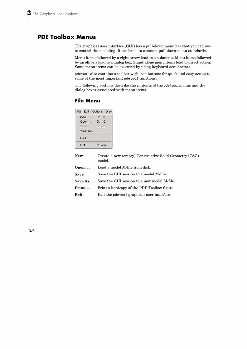
8/21/2019 matlab pde solving.pdf
http://slidepdf.com/reader/full/matlab-pde-solvingpdf 120/290
3-2
PDE Toolbox Menus
The graphical user interface (GUI) has a pull-down menu bar that you can useto control the modeling. It conforms to common pull-down menu standards.
Menu items followed by a right arrow lead to a submenu. Menu items followedby an ellipsis lead to a dialog box. Stand-alone menu items lead to direct action.Some menu items can be executed by using keyboard accelerators.
pdetool also contains a toolbar with icon buttons for quick and easy access to
some of the most important pdetool functions.The following sections describe the contents of the pdetool menus and thedialog boxes associated with menu items.
File Menu
New Create a new (empty) Constructive Solid Geometry (CSG)model.
Open. . . Load a model M-file from disk.
Save Save the GUI session to a model M-file.
Save As. . . Save the GUI session to a new model M-file.
Print. . . Print a hardcopy of the PDE Toolbox figure.
Exit Exit the pdetool graphical user interface.
PDE Toolbox Menus
New
8/21/2019 matlab pde solving.pdf
http://slidepdf.com/reader/full/matlab-pde-solvingpdf 121/290
3-3
New
New deletes the current CSG model and creates a new, empty model called“Untitled.”
Open . . .
Open . . . displays a dialog box with a list of existing M-files from which you canselect the file that you want to load. You can list the contents of a differentdirectory by changing the path in the Selection text box. You can use thescrollbar to display more filenames. You can select a file by double-clicking thefilename or by clicking the filename and then clicking the Done button. Whenyou select a file, the CSG model that is stored in the model M-file is loaded intothe PDE Toolbox and displayed. Also, the equation, the boundary conditions,and information about the mesh and the solution are loaded if present, and themodeling and solution process continues to the same status as when you savedthe file.
Save As . . .
Save As . . . displays a dialog box in which you can specify the name of the filein which to save the CSG model and other information regarding the GUIsession. You can also change the directory in which it is saved. If the filenameis given without a .m extension, .m is appended automatically.
The GUI session is stored in a model M-file, which contains a sequence ofdrawing commands and commands to recreate the modeling environment (axesscaling, grid, etc.). If you have already defined boundary conditions, PDEcoefficients, created a triangular mesh, and solved the PDE, further commandsto recreate the modeling and solution of the PDE problem are also included inthe model M-file. The pdetool GUI can be started from the command line byentering the name of a model M-file. The model in the file is then directlyloaded into the GUI.
3 The Graphical User Interface
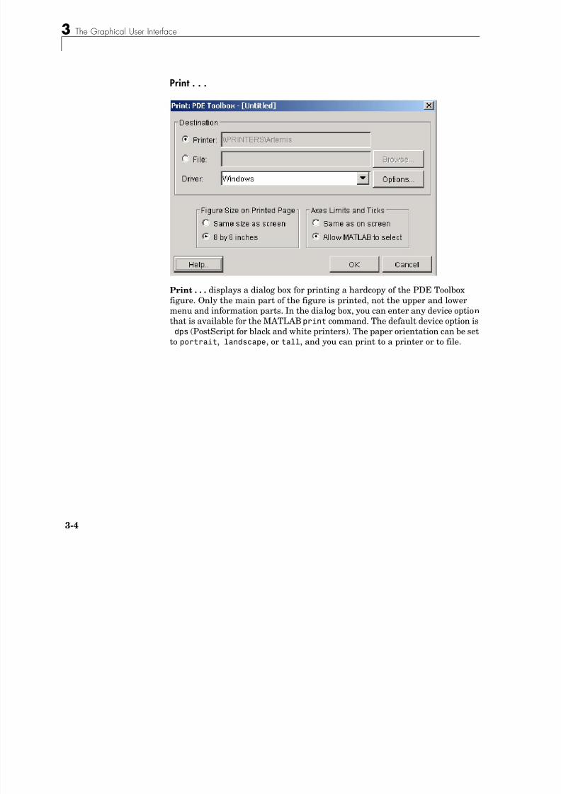
8/21/2019 matlab pde solving.pdf
http://slidepdf.com/reader/full/matlab-pde-solvingpdf 122/290
3-4
Print . . .
Print . . . displays a dialog box for printing a hardcopy of the PDE Toolboxfigure. Only the main part of the figure is printed, not the upper and lowermenu and information parts. In the dialog box, you can enter any device optionthat is available for the MATLAB print command. The default device option isdps (PostScript for black and white printers). The paper orientation can be set
to portrait, landscape, or tall, and you can print to a printer or to file.
PDE Toolbox Menus
Edit Menu
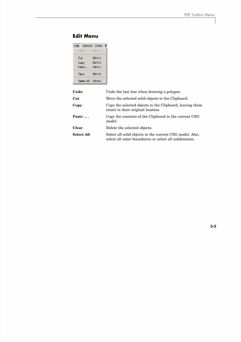
8/21/2019 matlab pde solving.pdf
http://slidepdf.com/reader/full/matlab-pde-solvingpdf 123/290
3-5
Edit Menu
Undo Undo the last line when drawing a polygon.
Cut Move the selected solid objects to the Clipboard.
Copy Copy the selected objects to the Clipboard, leaving themintact in their original location.
Paste . . . Copy the contents of the Clipboard to the current CSGmodel.
Clear Delete the selected objects.
Select All Select all solid objects in the current CSG model. Also,select all outer boundaries or select all subdomains.
3 The Graphical User Interface
Paste . . .

8/21/2019 matlab pde solving.pdf
http://slidepdf.com/reader/full/matlab-pde-solvingpdf 124/290
3-6
Paste . . .
Paste . . . displays a dialog box for pasting the contents of the Clipboard on tothe current CSG model. The Clipboard contents can be repeatedly pastedadding a specified x- and y-axis displacement to the positions of the Clipboardobjects.
Using the default values — zero displacement and one repetition — theClipboard contents is inserted at its original position.
PDE Toolbox Menus
Options Menu
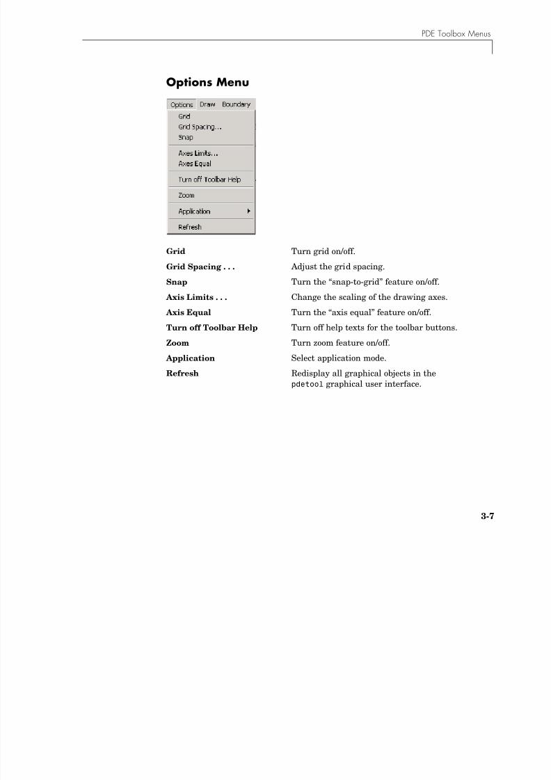
8/21/2019 matlab pde solving.pdf
http://slidepdf.com/reader/full/matlab-pde-solvingpdf 125/290
3-7
Options Menu
Grid Turn grid on/off.
Grid Spacing . . . Adjust the grid spacing.
Snap Turn the “snap-to-grid” feature on/off.
Axis Limits . . . Change the scaling of the drawing axes.
Axis Equal Turn the “axis equal” feature on/off.
Turn off Toolbar Help Turn off help texts for the toolbar buttons.
Zoom Turn zoom feature on/off. Application Select application mode.
Refresh Redisplay all graphical objects in thepdetool graphical user interface.
3 The Graphical User Interface
Grid Spacing . . .
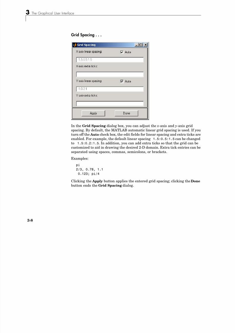
8/21/2019 matlab pde solving.pdf
http://slidepdf.com/reader/full/matlab-pde-solvingpdf 126/290
3-8
p g
In the Grid Spacing dialog box, you can adjust the x-axis and y-axis gridspacing. By default, the MATLAB automatic linear grid spacing is used. If youturn off the Auto check box, the edit fields for linear spacing and extra ticks areenabled. For example, the default linear spacing 1.5:0.5:1.5 can be changedto 1.5:0.2:1.5. In addition, you can add extra ticks so that the grid can be
customized to aid in drawing the desired 2-D domain. Extra tick entries can beseparated using spaces, commas, semicolons, or brackets.
Examples:
pi
2/3, 0.78, 1.1
0.123; pi/4
Clicking the Apply button applies the entered grid spacing; clicking the Done button ends the Grid Spacing dialog.
PDE Toolbox Menus
Axes Limits . . .
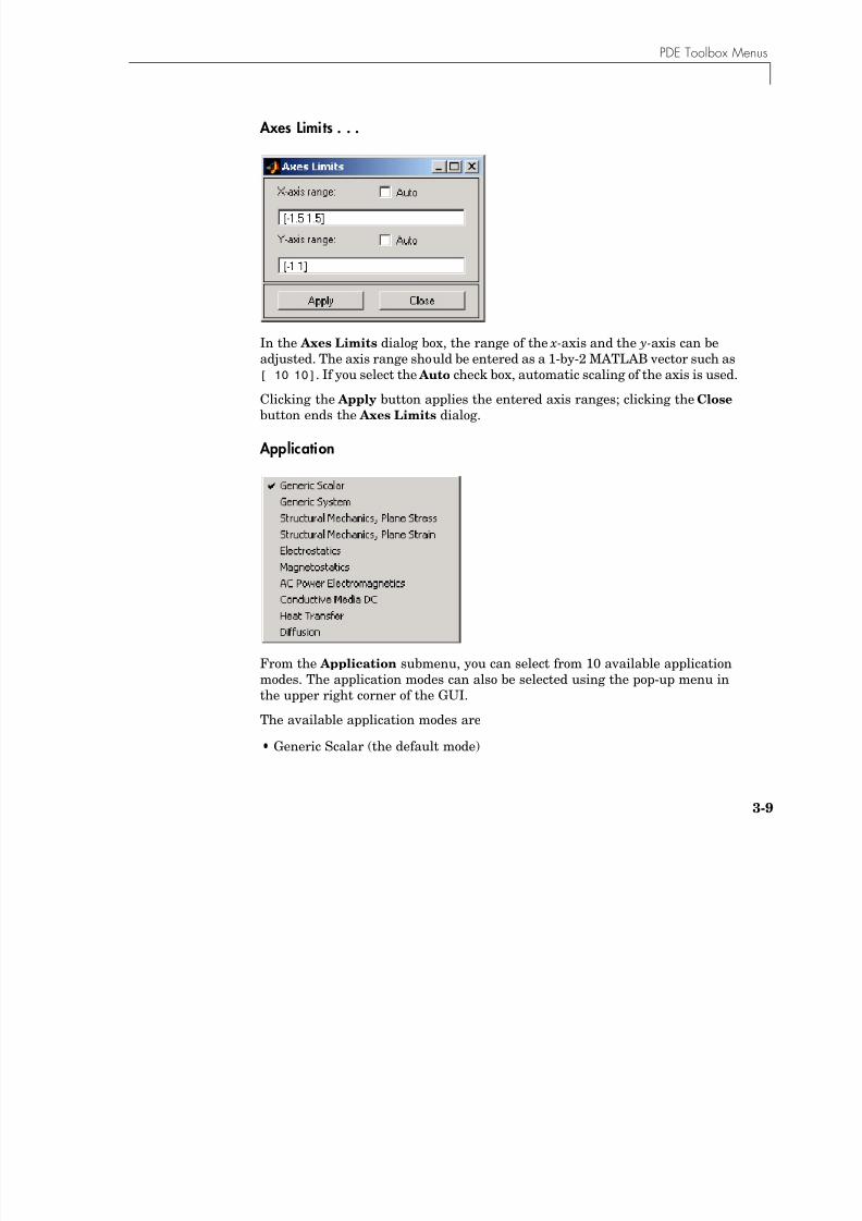
8/21/2019 matlab pde solving.pdf
http://slidepdf.com/reader/full/matlab-pde-solvingpdf 127/290
3-9
In the Axes Limits dialog box, the range of the x-axis and the y-axis can beadjusted. The axis range should be entered as a 1-by-2 MATLAB vector such as[ 10 10]. If you select the Auto check box, automatic scaling of the axis is used.
Clicking the Apply button applies the entered axis ranges; clicking the Close button ends the Axes Limits dialog.
Application
From the Application submenu, you can select from 10 available applicationmodes. The application modes can also be selected using the pop-up menu inthe upper right corner of the GUI.
The available application modes are
•Generic Scalar (the default mode)
3 The Graphical User Interface
•Generic System
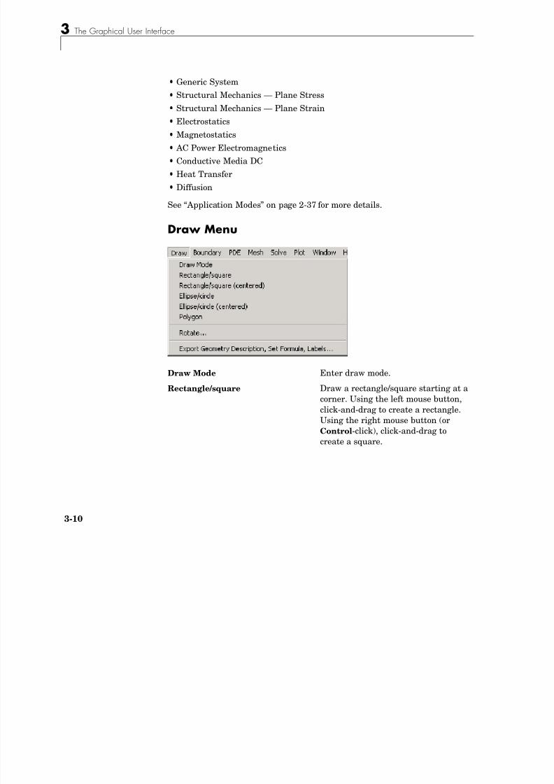
8/21/2019 matlab pde solving.pdf
http://slidepdf.com/reader/full/matlab-pde-solvingpdf 128/290
3-10
•Structural Mechanics — Plane Stress•Structural Mechanics — Plane Strain
•Electrostatics
•Magnetostatics
• AC Power Electromagnetics
•Conductive Media DC
•Heat Transfer
•Diffusion
See “Application Modes” on page 2-37 for more details.
Draw Menu
Draw Mode Enter draw mode.
Rectangle/square Draw a rectangle/square starting at acorner. Using the left mouse button,click-and-drag to create a rectangle.Using the right mouse button (orControl-click), click-and-drag tocreate a square.
PDE Toolbox Menus
Rectangle/square (centered) Draw a rectangle/square starting at
8/21/2019 matlab pde solving.pdf
http://slidepdf.com/reader/full/matlab-pde-solvingpdf 129/290
3-11
Rectangle/square (centered) Draw a rectangle/square starting at
the center. Using the left mousebutton, click-and-drag to create arectangle. Using the right mousebutton (or Control-click),click-and-drag to create a square.
Ellipse/circle Draw an ellipse/circle starting at theperimeter. Using the left mouse
button, click-and-drag to create anellipse. Using the right mouse button(or Control-click), click-and-drag tocreate a circle.
Ellipse/circle (centered) Draw an ellipse/circle starting at thecenter. Using the left mouse button,click-and-drag to create an ellipse.Using the right mouse button (orControl-click), click-and-drag tocreate a circle.
Polygon Draw a polygon. You can close thepolygon by pressing the right mousebutton. Clicking at the starting vertexalso closes the polygon.
Rotate . . . Rotate selected objects.
Export Geometry Description, Set
Formula, Labels. . .
Export the Geometry Descriptionmatrix gd, the set formula string sf,and the Name Space matrix ns (labels)to the main workspace.
3 The Graphical User Interface
Rotate . . .

8/21/2019 matlab pde solving.pdf
http://slidepdf.com/reader/full/matlab-pde-solvingpdf 130/290
3-12
Rotate . . . opens a dialog box where you can enter the angle of rotation indegrees. The selected objects are then rotated by the number of degrees thatyou specify. The rotation is done counter clockwise for positive rotation angles.
By default, the rotation center is the center-of-mass of the selected objects. Ifthe Use center-of-mass option is not selected, you can enter a rotation center( xc ,yc) as a 1-by-2 MATLAB vector such as [ 0.4 0.3].
PDE Toolbox Menus
Boundary Menu

8/21/2019 matlab pde solving.pdf
http://slidepdf.com/reader/full/matlab-pde-solvingpdf 131/290
3-13
y
Boundary Mode Enter the boundary mode.
Specify Boundary
Conditions . . .
Specify boundary conditions for the selectedboundaries. If no boundaries are selected, theentered boundary condition applies to all
boundaries.Show Edge Labels Toggle the labeling of the edges (outer
boundaries and subdomain borders) on/off.The edges are labeled using the columnnumber in the Decomposed Geometry matrix.
Show Subdomains
Labels
Toggle the labeling of the subdomains on/off.The subdomains are labeled using the
subdomain numbering in the DecomposedGeometry matrix.
Remove Subdomain Border Remove selected subdomain borders.
Remove All Subdomain
Borders
Remove all subdomain borders.
Export Decomposed
Geometry, Boundary Cond’s
. . .
Export the Decomposed Geometry matrix g and the Boundary Condition matrix b to themain workspace.
3 The Graphical User Interface
Specify Boundary Conditions . . .
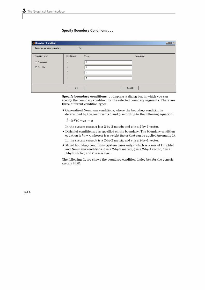
8/21/2019 matlab pde solving.pdf
http://slidepdf.com/reader/full/matlab-pde-solvingpdf 132/290
3-14
Specify boundary conditions . . . displays a dialog box in which you canspecify the boundary condition for the selected boundary segments. There arethree different condition types:
•Generalized Neumann conditions, where the boundary condition isdetermined by the coefficients q and g according to the following equation:
In the system cases, q is a 2-by-2 matrix and g is a 2-by-1 vector.•Dirichlet conditions: u is specified on the boundary. The boundary condition
equation is hu = r, where h is a weight factor that can be applied (normally 1).
In the system cases, h is a 2-by-2 matrix and r is a 2-by-1 vector.
•Mixed boundary conditions (system cases only), which is a mix of Dirichletand Neumann conditions. q is a 2-by-2 matrix, g is a 2-by-1 vector, h is a1-by-2 vector, and r is a scalar.
The following figure shows the boundary condition dialog box for the genericsystem PDE.
n c u∇( )⋅ qu+ g=
PDE Toolbox Menus
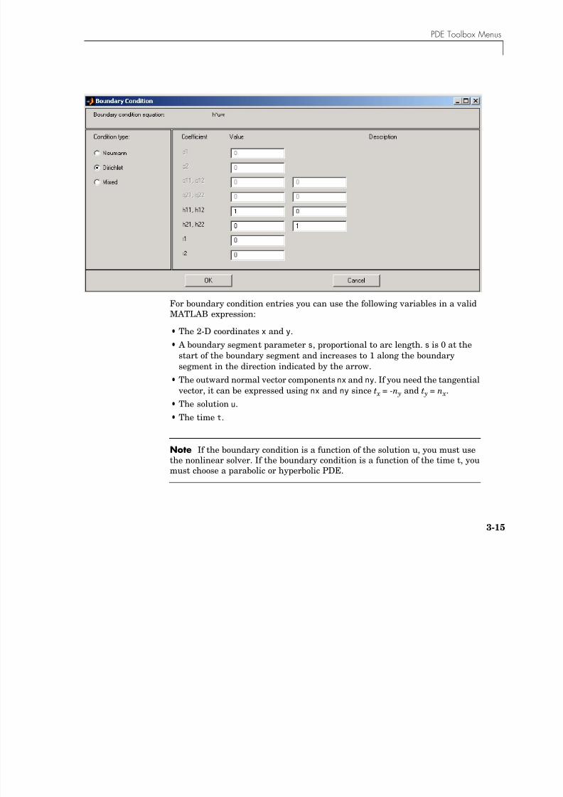
8/21/2019 matlab pde solving.pdf
http://slidepdf.com/reader/full/matlab-pde-solvingpdf 133/290
3-15
For boundary condition entries you can use the following variables in a validMATLAB expression:
•The 2-D coordinates x and y.
• A boundary segment parameter s, proportional to arc length. s is 0 at thestart of the boundary segment and increases to 1 along the boundarysegment in the direction indicated by the arrow.
•The outward normal vector components nx and ny. If you need the tangential vector, it can be expressed using nx and ny since t x = -n y and t y = n x.
•The solution u.
•The time t.
Note If the boundary condition is a function of the solution u, you must usethe nonlinear solver. If the boundary condition is a function of the time t, youmust choose a parabolic or hyperbolic PDE.
3 The Graphical User Interface
Examples: (100 80*s).*nx, and cos(x.^2)
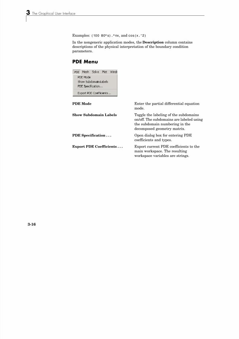
8/21/2019 matlab pde solving.pdf
http://slidepdf.com/reader/full/matlab-pde-solvingpdf 134/290
3-16
In the nongeneric application modes, the Description column containsdescriptions of the physical interpretation of the boundary conditionparameters.
PDE Menu
PDE Mode Enter the partial differential equationmode.
Show Subdomain Labels Toggle the labeling of the subdomainson/off. The subdomains are labeled usingthe subdomain numbering in thedecomposed geometry matrix.
PDE Specification . . . Open dialog box for entering PDEcoefficients and types.
Export PDE Coefficients . . . Export current PDE coefficients to the
main workspace. The resultingworkspace variables are strings.
PDE Toolbox Menus
PDE Specification . . .
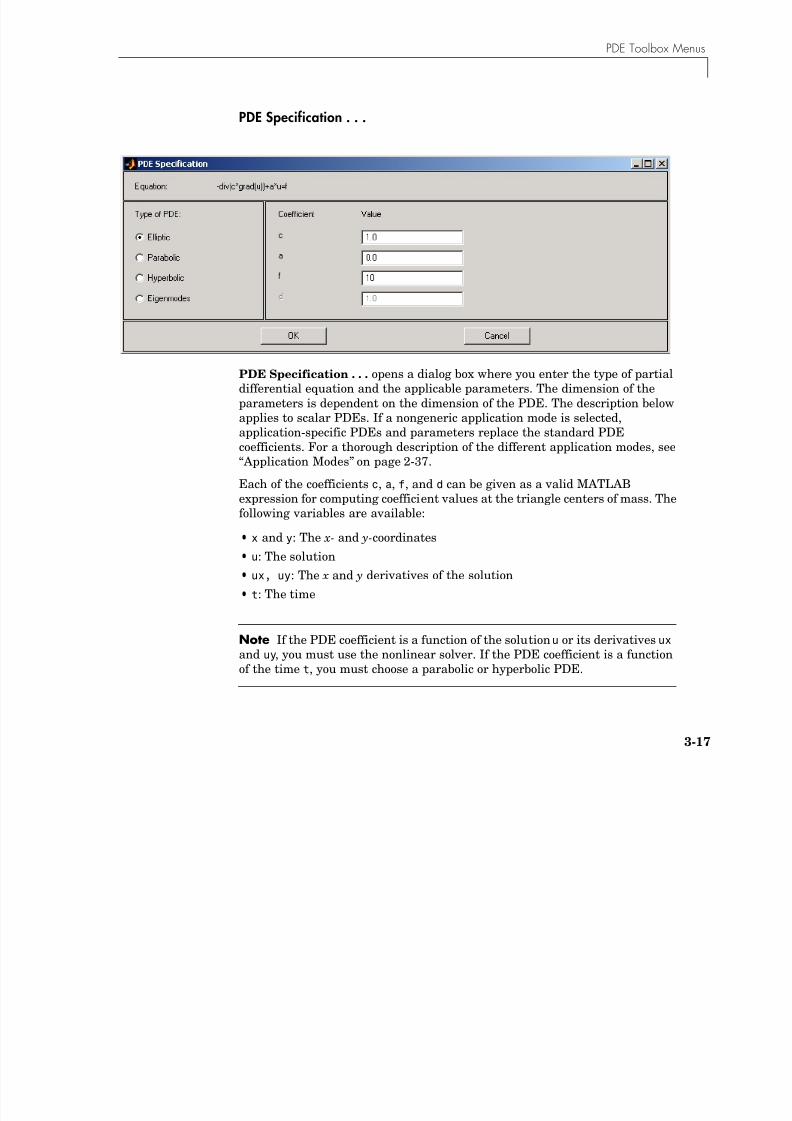
8/21/2019 matlab pde solving.pdf
http://slidepdf.com/reader/full/matlab-pde-solvingpdf 135/290
3-17
PDE Specification . . . opens a dialog box where you enter the type of partialdifferential equation and the applicable parameters. The dimension of theparameters is dependent on the dimension of the PDE. The description belowapplies to scalar PDEs. If a nongeneric application mode is selected,application-specific PDEs and parameters replace the standard PDEcoefficients. For a thorough description of the different application modes, see“Application Modes” on page 2-37.
Each of the coefficients c, a, f, and d can be given as a valid MATLAB
expression for computing coefficient values at the triangle centers of mass. Thefollowing variables are available:
• x and y: The x- and y-coordinates
• u: The solution
• ux, uy: The x and y derivatives of the solution
• t: The time
Note If the PDE coefficient is a function of the solution u or its derivatives uxand uy, you must use the nonlinear solver. If the PDE coefficient is a functionof the time t, you must choose a parabolic or hyperbolic PDE.
3 The Graphical User Interface
You can also enter the name of a user-defined MATLAB function that acceptsthe arguments (p t u time) For an example type the function circlef
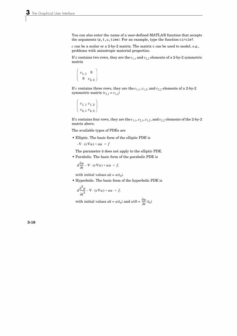
8/21/2019 matlab pde solving.pdf
http://slidepdf.com/reader/full/matlab-pde-solvingpdf 136/290
3-18
the arguments (p,t,u,time). For an example, type the function circlef.
c can be a scalar or a 2-by-2 matrix. The matrix c can be used to model, e.g.,problems with anisotropic material properties.
If c contains two rows, they are the c1,1 and c2,2 elements of a 2-by-2 symmetricmatrix
If c contains three rows, they are the c1,1, c1,2, and c2,2 elements of a 2-by-2symmetric matrix (c2,1 = c1,2)
If c contains four rows, they are the c1,1, c2,1, c1,2, and c2,2 elements of the 2-by-2matrix above.
The available types of PDEs are
•Elliptic. The basic form of the elliptic PDE is
The parameter d does not apply to the elliptic PDE.
•Parabolic. The basic form of the parabolic PDE is
with initial values u0 = u(t0).
•Hyperbolic. The basic form of the hyperbolic PDE is
with initial values u0 = u(t0) and ut0 = (t0)
c1 1, 0
0 c2 2,# $% &
% &' (
c1 1, c1 2,
c2 1, c2 2,# $% &% &' (
∇ – c∇u( )⋅ au+ f =
d∂u
∂t------ ∇ – c∇u( )⋅ au+ f ,=
d∂
2u
∂t2
--------- ∇ – c∇u( )⋅ au+ f ,=
∂u
∂t------
PDE Toolbox Menus
•Eigenmodes. The basic form of the PDE eigenvalue problem is
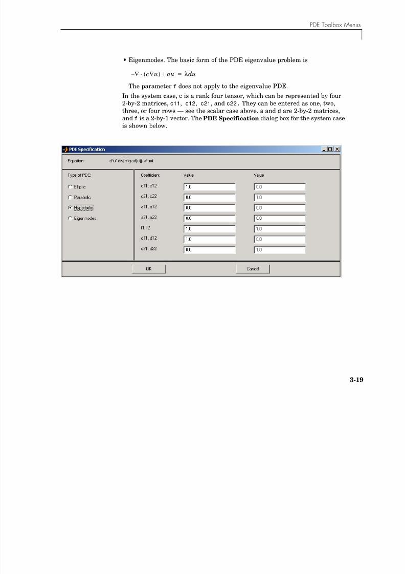
8/21/2019 matlab pde solving.pdf
http://slidepdf.com/reader/full/matlab-pde-solvingpdf 137/290
3-19
The parameter f does not apply to the eigenvalue PDE.
In the system case, c is a rank four tensor, which can be represented by four2-by-2 matrices, c11, c12, c21, and c22. They can be entered as one, two,three, or four rows — see the scalar case above. a and d are 2-by-2 matrices,and f is a 2-by-1 vector. The PDE Specification dialog box for the system caseis shown below.
∇ – c∇u( )⋅ au+ λdu=
3 The Graphical User Interface
Mesh Menu
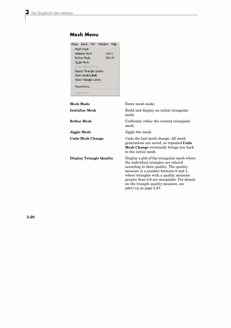
8/21/2019 matlab pde solving.pdf
http://slidepdf.com/reader/full/matlab-pde-solvingpdf 138/290
3-20
Mesh Mode Enter mesh mode.
Initialize Mesh Build and display an initial triangularmesh.
Refine Mesh Uniformly refine the current triangularmesh.
Jiggle Mesh Jiggle the mesh.
Undo Mesh Change Undo the last mesh change. All meshgenerations are saved, so repeated Undo
Mesh Change eventually brings you backto the initial mesh.
Display Triangle Quality Display a plot of the triangular mesh wherethe individual triangles are coloredaccording to their quality. The qualitymeasure is a number between 0 and 1,where triangles with a quality measure
greater than 0.6 are acceptable. For detailson the triangle quality measure, seepdetriq on page 5-87.
PDE Toolbox Menus
Show Node Labels Toggle the mesh node labels on/off. The
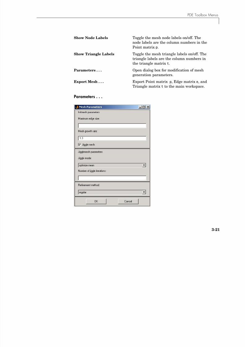
8/21/2019 matlab pde solving.pdf
http://slidepdf.com/reader/full/matlab-pde-solvingpdf 139/290
3-21
Parameters . . .
node labels are the column numbers in thePoint matrix p.
Show Triangle Labels Toggle the mesh triangle labels on/off. Thetriangle labels are the column numbers inthe triangle matrix t.
Parameters . . . Open dialog box for modification of meshgeneration parameters.
Export Mesh . . . Export Point matrix p, Edge matrix e, andTriangle matrix t to the main workspace.
3 The Graphical User Interface
Parameters . . . opens a dialog box containing mesh generation parameters.The parameters used by the mesh initialization algorithm initmesh are
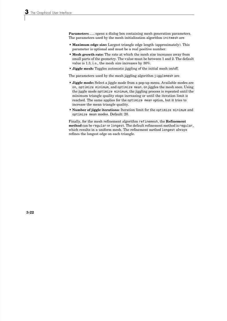
8/21/2019 matlab pde solving.pdf
http://slidepdf.com/reader/full/matlab-pde-solvingpdf 140/290
3-22
p y g
•Maximum edge size: Largest triangle edge length (approximately). Thisparameter is optional and must be a real positive number.
•Mesh growth rate: The rate at which the mesh size increases away fromsmall parts of the geometry. The value must be between 1 and 2. The default value is 1.3, i.e., the mesh size increases by 30%.
•Jiggle mesh: Toggles automatic jiggling of the initial mesh on/off.
The parameters used by the mesh jiggling algorithm jigglemesh are
•Jiggle mode: Select a jiggle mode from a pop-up menu. Available modes areon, optimize minimum, and optimize mean. on jiggles the mesh once. Usingthe jiggle mode optimize minimum, the jiggling process is repeated until theminimum triangle quality stops increasing or until the iteration limit isreached. The same applies for the optimize mean option, but it tries toincrease the mean triangle quality.
•Number of jiggle iterations: Iteration limit for the optimize minimum andoptimize mean modes. Default: 20.
Finally, for the mesh refinement algorithm refinemesh, the Refinement
method can be regular or longest. The default refinement method is regular,which results in a uniform mesh. The refinement method longest alwaysrefines the longest edge on each triangle.
PDE Toolbox Menus
Solve Menu
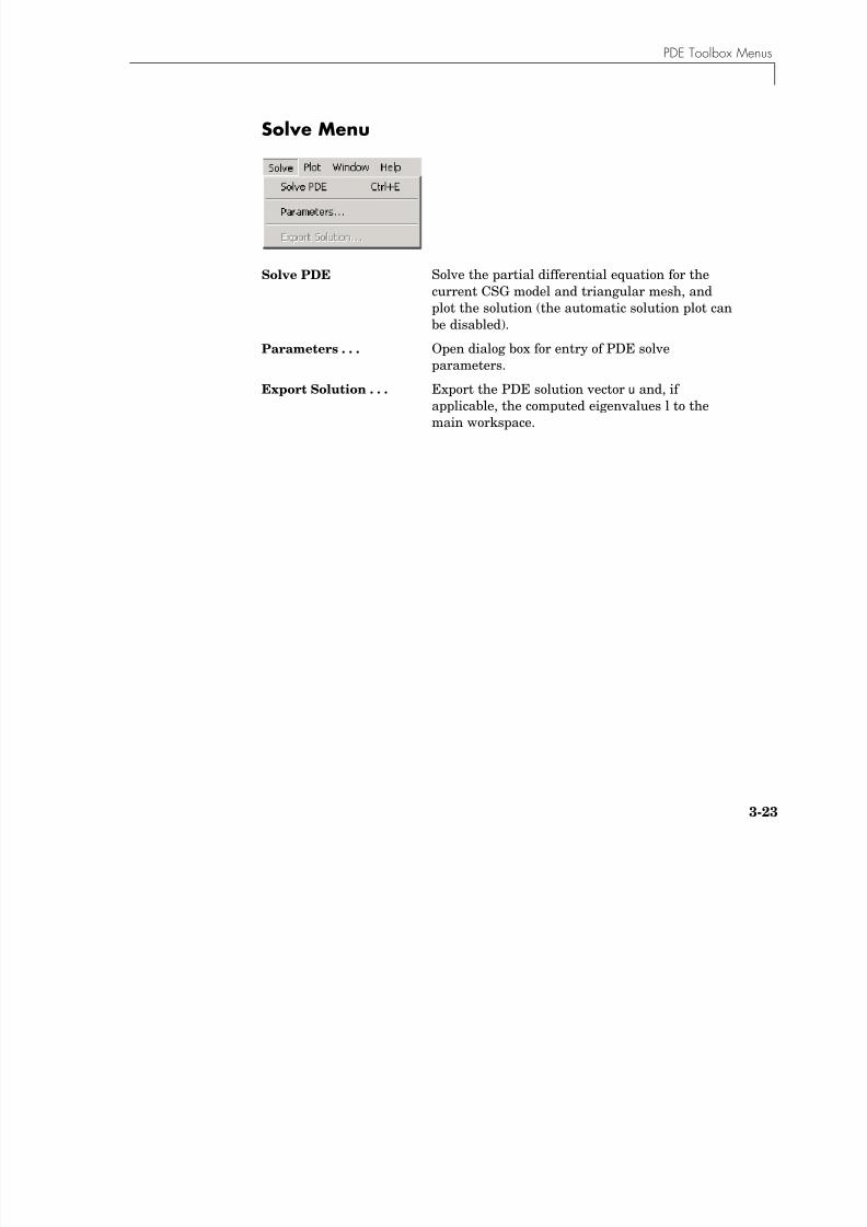
8/21/2019 matlab pde solving.pdf
http://slidepdf.com/reader/full/matlab-pde-solvingpdf 141/290
3-23
Solve PDE Solve the partial differential equation for thecurrent CSG model and triangular mesh, andplot the solution (the automatic solution plot canbe disabled).
Parameters . . . Open dialog box for entry of PDE solveparameters.
Export Solution . . . Export the PDE solution vector u and, if
applicable, the computed eigenvalues l to themain workspace.
3 The Graphical User Interface
Parameters . . .
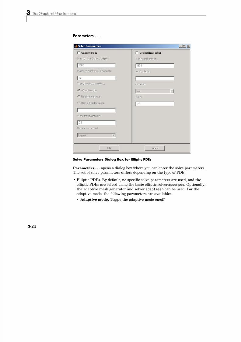
8/21/2019 matlab pde solving.pdf
http://slidepdf.com/reader/full/matlab-pde-solvingpdf 142/290
3-24
Solve Parameters Dialog Box for Elliptic PDEs
Parameters . . . opens a dialog box where you can enter the solve parameters.The set of solve parameters differs depending on the type of PDE.
•Elliptic PDEs. By default, no specific solve parameters are used, and theelliptic PDEs are solved using the basic elliptic solver assempde. Optionally,
the adaptive mesh generator and solver adaptmesh can be used. For theadaptive mode, the following parameters are available:
- Adaptive mode. Toggle the adaptive mode on/off.
PDE Toolbox Menus
- Maximum number of triangles. The maximum number of new trianglesallowed (can be set to Inf). A default value is calculated based on the

8/21/2019 matlab pde solving.pdf
http://slidepdf.com/reader/full/matlab-pde-solvingpdf 143/290
3-25
current mesh.
- Maximum number of refinements. The maximum number of successiverefinements attempted.
- Triangle selection method. Two triangle selection methods are includedin the PDE Toolbox. You can also supply your own function.
- Worst triangles. This method picks all triangles that are worse than afraction of the value of the worst triangle (default: 0.5). For more details,see pdeadworst on page 5-48.
- Relative tolerance. This method picks triangles using a relative toler-ance criterion (default: 1E-3). For more details, see pdeadgsc onpage 5-47.
- User-defined function. Enter the name of a user-defined triangle selec-tion method. See pdedemo7 for an example of a user-defined triangle
selection method.- Function parameter. The function parameter allows fine-tuning of the
triangle selection methods. For the worst triangle method (pdeadworst), itis the fraction of the worst value that is used to determine which trianglesto refine. For the relative tolerance method, it is a tolerance parameterthat controls how well the solution fits the PDE.
- Refinement method. Can be regular or longest. See the Parameters. . .
dialog box description in “Mesh Menu” on page 3-20. If the problem is nonlinear, i.e., parameters in the PDE are directly dependenton the solution u, a nonlinear solver must be used. The following parametersare used:
- Use nonlinear solver. Toggle the nonlinear solver on/off.
- Nonlinear tolerance. Tolerance parameter for the nonlinear solver.
3 The Graphical User Interface
- Initial solution. An initial guess. Can be a constant or a function of x and y given as a MATLAB expression that can be evaluated on the nodes of the
8/21/2019 matlab pde solving.pdf
http://slidepdf.com/reader/full/matlab-pde-solvingpdf 144/290
3-26
current mesh.
Examples: 1, and exp(x.*y). Optional parameter, defaults to zero.
- Jacobian. Jacobian approximation method: fixed (the default), a fixedpoint iteration, lumped, a “lumped” (diagonal) approximation, or full, thefull Jacobian.
- Norm. The type of norm used for computing the residual. Enter as energy
for an energy norm, or as a real scalar p
to give thel p norm. The default isInf, the infinity (maximum) norm.
Note The adaptive mode and the nonlinear solver can be used together.
•Parabolic PDEs. The solve parameters for the parabolic PDEs are
- Time. A MATLAB vector of times at which a solution to the parabolic PDEshould be generated. The relevant time span is dependent on the dynamicsof the problem.
Examples: 0:10, and logspace( 2,0,20)
- u(t0). The initial value u(t0) for the parabolic PDE problem The initial value can be a constant or a column vector of values on the nodes of thecurrent mesh.
- Relative tolerance.
Relative tolerance parameter for the ODE solver thatis used for solving the time-dependent part of the parabolic PDE problem.
- Absolute tolerance. Absolute tolerance parameter for the ODE solverthat is used for solving the time-dependent part of the parabolic PDEproblem.
PDE Toolbox Menus

8/21/2019 matlab pde solving.pdf
http://slidepdf.com/reader/full/matlab-pde-solvingpdf 145/290
3-27
Solve Parameters Dialog Box for Hyperbolic PDEs
•Hyperbolic PDEs. The solve parameters for the hyperbolic PDEs are
- Time. A MATLAB vector of times at which a solution to the hyperbolicPDE should be generated. The relevant time span is dependent on thedynamics of the problem.
Examples: 0:10, and logspace( 2,0,20)
- u(t0). The initial value u(t0) for the hyperbolic PDE problem. The initial
value can be a constant or a column vector of values on the nodes of thecurrent mesh.
- u’(t0). The initial value (t0) for the hyperbolic PDE problem. You can usethe same formats as for u(t0).
- Relative tolerance. Relative tolerance parameter for the ODE solver thatis used for solving the time-dependent part of the hyperbolic PDE problem.
- Absolute tolerance. Absolute tolerance parameter for the ODE solver
that is used for solving the time-dependent part of the hyperbolic PDEproblem.
u·
3 The Graphical User Interface
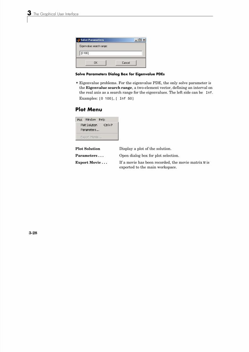
8/21/2019 matlab pde solving.pdf
http://slidepdf.com/reader/full/matlab-pde-solvingpdf 146/290
3-28
Solve Parameters Dialog Box for Eigenvalue PDEs
•Eigenvalue problems. For the eigenvalue PDE, the only solve parameter isthe Eigenvalue search range, a two-element vector, defining an interval onthe real axis as a search range for the eigenvalues. The left side can be Inf.
Examples: [0 100], [ Inf 50]
Plot Menu
Plot Solution Display a plot of the solution.
Parameters . . . Open dialog box for plot selection.Export Movie . . . If a movie has been recorded, the movie matrix M is
exported to the main workspace.
PDE Toolbox Menus
Parameters . . .
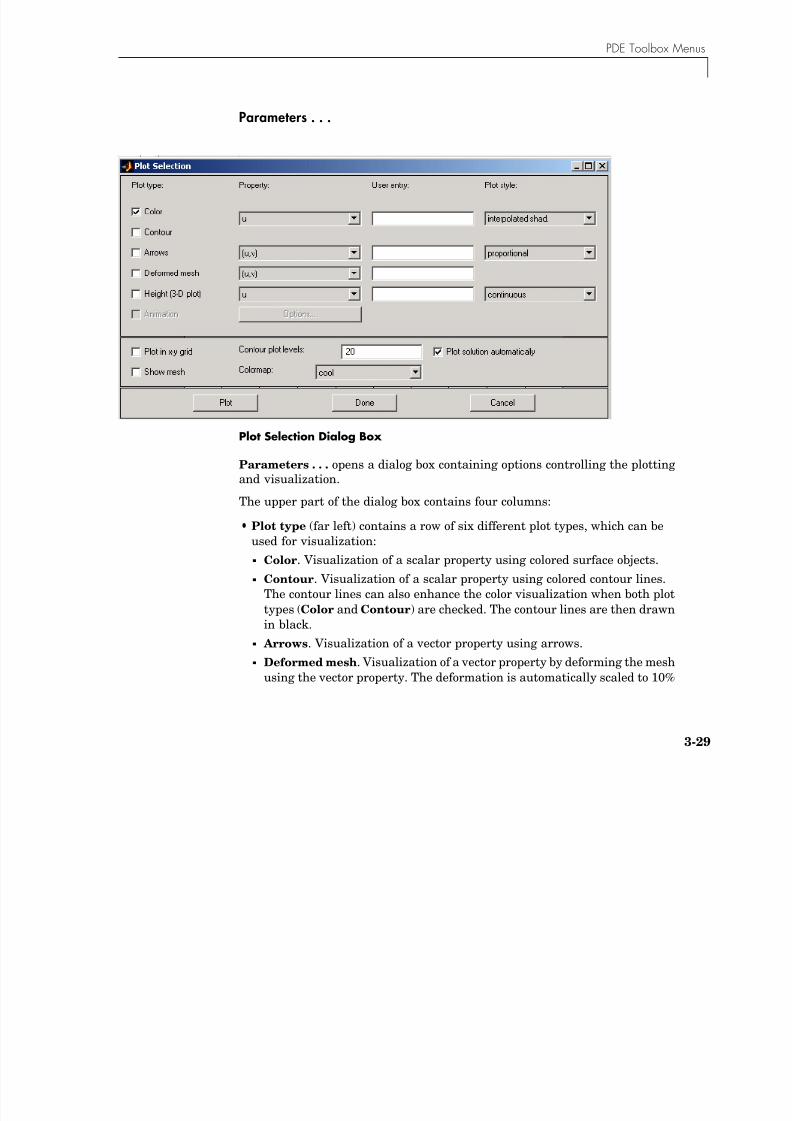
8/21/2019 matlab pde solving.pdf
http://slidepdf.com/reader/full/matlab-pde-solvingpdf 147/290
3-29
Plot Selection Dialog Box
Parameters . . . opens a dialog box containing options controlling the plottingand visualization.
The upper part of the dialog box contains four columns:
•Plot type (far left) contains a row of six different plot types, which can beused for visualization:
- Color. Visualization of a scalar property using colored surface objects.
- Contour. Visualization of a scalar property using colored contour lines.The contour lines can also enhance the color visualization when both plottypes (Color and Contour) are checked. The contour lines are then drawnin black.
- Arrows. Visualization of a vector property using arrows.
- Deformed mesh. Visualization of a vector property by deforming the meshusing the vector property. The deformation is automatically scaled to 10%
3 The Graphical User Interface
of the problem domain. This plot type is primarily intended for visualizing x- and y-displacements (u and v) for problems in structural mechanics. If
th l t t i l t d th d f d t i l h i di l d
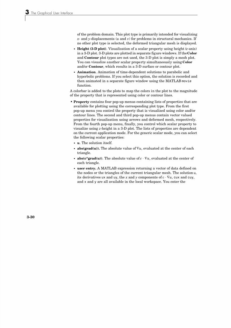
8/21/2019 matlab pde solving.pdf
http://slidepdf.com/reader/full/matlab-pde-solvingpdf 148/290
3-30
no other plot type is selected, the deformed triangular mesh is displayed.- Height (3-D plot). Visualization of a scalar property using height ( z-axis)
in a 3-D plot. 3-D plots are plotted in separate figure windows. If the Color and Contour plot types are not used, the 3-D plot is simply a mesh plot. You can visualize another scalar property simultaneously using Color and/or Contour, which results in a 3-D surface or contour plot.
- Animation. Animation of time-dependent solutions to parabolic and
hyperbolic problems. If you select this option, the solution is recorded andthen animated in a separate figure window using the MATLAB movie function.
A colorbar is added to the plots to map the colors in the plot to the magnitudeof the property that is represented using color or contour lines.
•Property contains four pop-up menus containing lists of properties that areavailable for plotting using the corresponding plot type. From the first
pop-up menu you control the property that is visualized using color and/orcontour lines. The second and third pop-up menus contain vector valuedproperties for visualization using arrows and deformed mesh, respectively.From the fourth pop-up menu, finally, you control which scalar property to visualize using z-height in a 3-D plot. The lists of properties are dependenton the current application mode. For the generic scalar mode, you can selectthe following scalar properties:
- u. The solution itself.
- abs(grad(u)). The absolute value of ∇u, evaluated at the center of eachtriangle.
- abs(c*grad(u)). The absolute value of c ⋅ ∇u, evaluated at the center ofeach triangle.
- user entry. A MATLAB expression returning a vector of data defined onthe nodes or the triangles of the current triangular mesh. The solution u,its derivatives ux and uy, the x and y components of c ⋅ ∇u, cux and cuy,
and x and y are all available in the local workspace. You enter the
PDE Toolbox Menus
expression into the edit box to the right of the Property pop-up menu inthe User entry column.
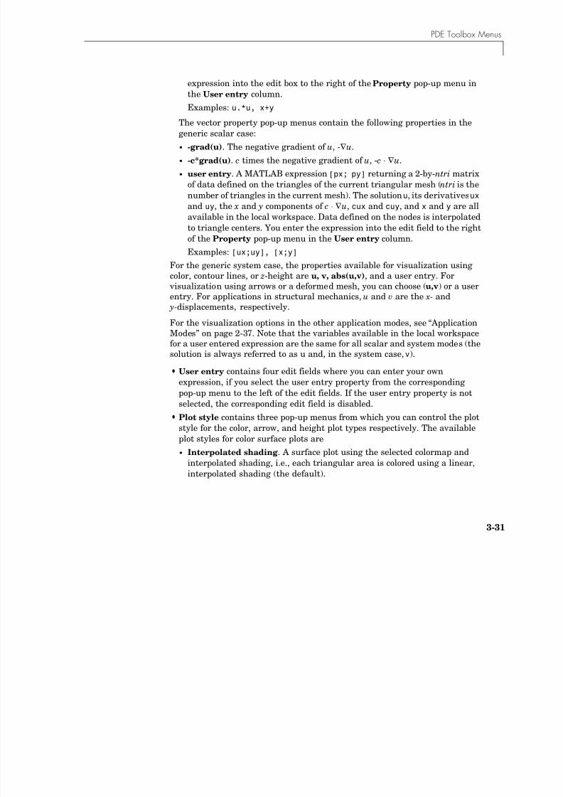
8/21/2019 matlab pde solving.pdf
http://slidepdf.com/reader/full/matlab-pde-solvingpdf 149/290
3-31
Examples: u.*u, x+y
The vector property pop-up menus contain the following properties in thegeneric scalar case:
- -grad(u). The negative gradient of u, -∇u.
- -c*grad(u). c times the negative gradient of u, -c ⋅ ∇u.
- user entry. A MATLAB expression [px; py] returning a 2-by-ntri matrix
of data defined on the triangles of the current triangular mesh (ntri is thenumber of triangles in the current mesh). The solution u, its derivativesux and uy, the x and y components of c ⋅ ∇u, cux and cuy, and x and y are allavailable in the local workspace. Data defined on the nodes is interpolatedto triangle centers. You enter the expression into the edit field to the rightof the Property pop-up menu in the User entry column.
Examples: [ux;uy], [x;y]
For the generic system case, the properties available for visualization usingcolor, contour lines, or z-height are u, v, abs(u,v), and a user entry. For visualization using arrows or a deformed mesh, you can choose (u,v) or a userentry. For applications in structural mechanics, u and v are the x- and y-displacements, respectively.
For the visualization options in the other application modes, see “ApplicationModes” on page 2-37. Note that the variables available in the local workspacefor a user entered expression are the same for all scalar and system modes (the
solution is always referred to as u and, in the system case, v).•User entry contains four edit fields where you can enter your own
expression, if you select the user entry property from the correspondingpop-up menu to the left of the edit fields. If the user entry property is notselected, the corresponding edit field is disabled.
•Plot style contains three pop-up menus from which you can control the plotstyle for the color, arrow, and height plot types respectively. The available
plot styles for color surface plots are- Interpolated shading . A surface plot using the selected colormap and
interpolated shading, i.e., each triangular area is colored using a linear,interpolated shading (the default).
3 The Graphical User Interface
- Flat shading . A surface plot using the selected colormap and flat shading,i.e., each triangular area is colored using a constant color.
d ff l l
8/21/2019 matlab pde solving.pdf
http://slidepdf.com/reader/full/matlab-pde-solvingpdf 150/290
3-32
You can use two different arrow plot styles:
- Proportional. The length of the arrow corresponds to the magnitude ofthe property that you visualize (the default).
- Normalized. The lengths of all arrows are normalized, i.e., all arrows havethe same length. This is useful when you are interested in the direction ofthe vector field. The direction is clearly visible even in areas where themagnitude of the field is very small.
For height (3-D plots), the available plot styles are
- Continuous. Produces a “smooth” continuous plot by interpolating datafrom triangle midpoints to the mesh nodes (the default).
- Discontinuous. Produces a discontinuous plot where data and z-heightare constant on each triangle.
A total of three properties of the solution — two scalar properties and one vector field — can be visualized simultaneously. If the Height (3-D plot) optionis turned off, the solution plot is a 2-D plot and is plotted in the main axes ofthe pdetool GUI. If the Height (3-D plot) option is used, the solution plot is a3-D plot in a separate figure window. If possible, the 3-D plot uses an existingfigure window. If you would like to plot in a new figure window, simply typefigure at the MATLAB command line.
Additional Plot Control Options
In the middle of the dialog box are a number of additional plot control options:•Plot in x–y grid. If you select this option, the solution is converted from the
original triangular grid to a rectangular x-y grid. This is especially useful foranimations since it speeds up the process of recording the movie framessignificantly.
•Show mesh. In the surface plots, the mesh is plotted using black color if youselect this option. By default, the mesh is hidden.
•Contour plot levels. For contour plots, the number of level curves, e.g., 15 or 20 can be entered. Alternatively, you can enter a MATLAB vector of levels.The curves of the contour plot are then drawn at those levels. The default is20 contour level curves.
Examples: [0:100:1000], logspace( 1,1,30)
PDE Toolbox Menus
•Colormap. Using the Colormap pop-up menu, you can select from a numberof different colormaps: cool, gray, bone, pink, copper, hot, jet, hsv, andprism
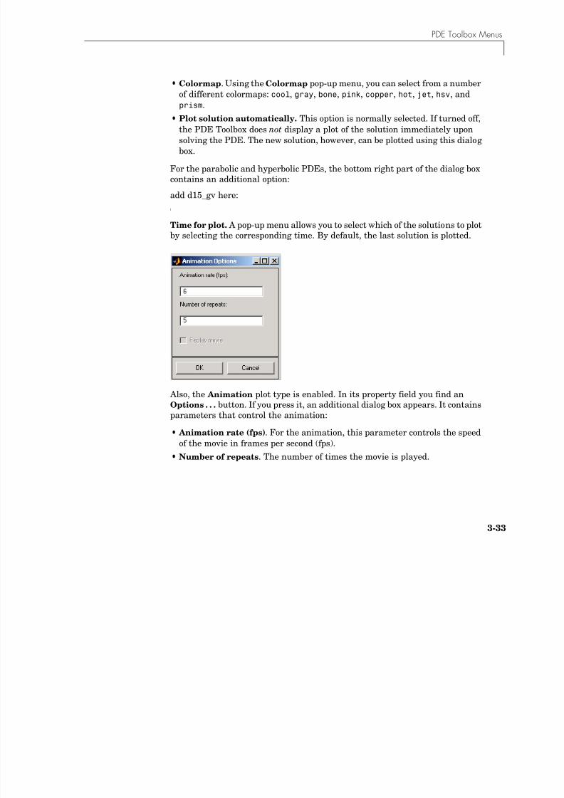
8/21/2019 matlab pde solving.pdf
http://slidepdf.com/reader/full/matlab-pde-solvingpdf 151/290
3-33
prism.•Plot solution automatically. This option is normally selected. If turned off,
the PDE Toolbox does not display a plot of the solution immediately uponsolving the PDE. The new solution, however, can be plotted using this dialogbox.
For the parabolic and hyperbolic PDEs, the bottom right part of the dialog boxcontains an additional option:
add d15_gv here:(
Time for plot. A pop-up menu allows you to select which of the solutions to plotby selecting the corresponding time. By default, the last solution is plotted.
Also, the Animation plot type is enabled. In its property field you find anOptions . . . button. If you press it, an additional dialog box appears. It containsparameters that control the animation:
• Animation rate (fps). For the animation, this parameter controls the speedof the movie in frames per second (fps).
•Number of repeats. The number of times the movie is played.
3 The Graphical User Interface
•Replay movie. If you select this option, the current movie is replayedwithout rerecording the movie frames. If there is no current movie, thisoption is disabled
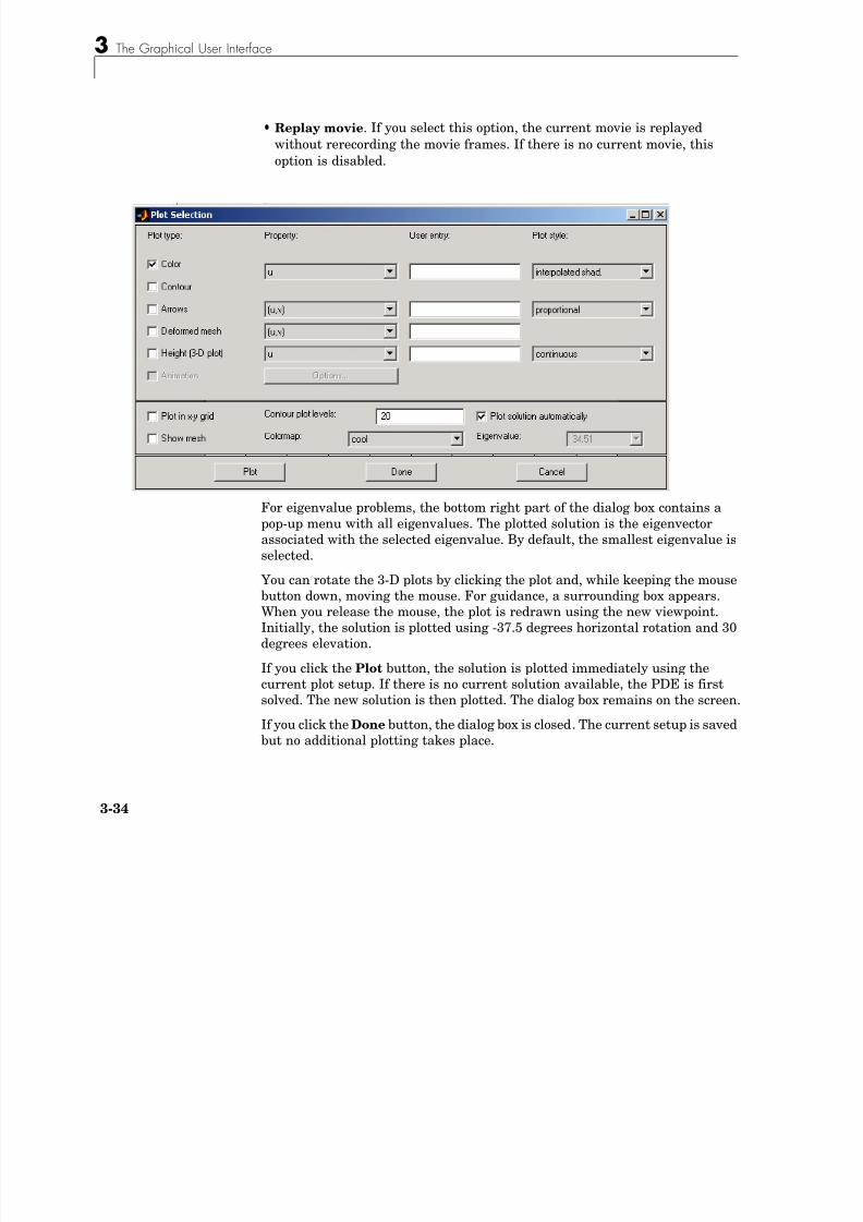
8/21/2019 matlab pde solving.pdf
http://slidepdf.com/reader/full/matlab-pde-solvingpdf 152/290
3-34
option is disabled.
For eigenvalue problems, the bottom right part of the dialog box contains apop-up menu with all eigenvalues. The plotted solution is the eigenvector
associated with the selected eigenvalue. By default, the smallest eigenvalue isselected.
You can rotate the 3-D plots by clicking the plot and, while keeping the mousebutton down, moving the mouse. For guidance, a surrounding box appears.When you release the mouse, the plot is redrawn using the new viewpoint.Initially, the solution is plotted using -37.5 degrees horizontal rotation and 30degrees elevation.
If you click the Plot button, the solution is plotted immediately using thecurrent plot setup. If there is no current solution available, the PDE is firstsolved. The new solution is then plotted. The dialog box remains on the screen.
If you click the Done button, the dialog box is closed. The current setup is savedbut no additional plotting takes place.
PDE Toolbox Menus
If you click the Cancel button, the dialog box is closed. The setup remainsunchanged since the last plot.
8/21/2019 matlab pde solving.pdf
http://slidepdf.com/reader/full/matlab-pde-solvingpdf 153/290
3-35
Window MenuFrom the Window menu, you can select all currently open MATLAB figurewindows. The selected window is brought to the front.
Help Menu
Help . . . Display a brief help window. About . . . Display a window with some program information.
3 The Graphical User Interface
The Toolbar
The toolbar underneath the main menu at the top of the GUI contains icon
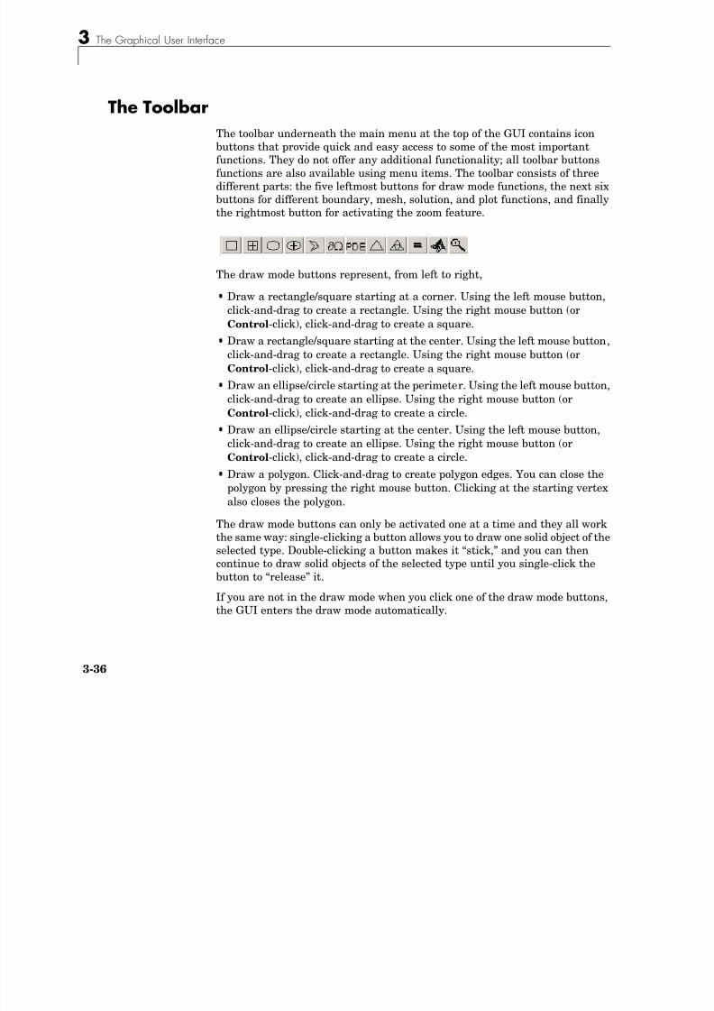
8/21/2019 matlab pde solving.pdf
http://slidepdf.com/reader/full/matlab-pde-solvingpdf 154/290
3-36
The toolbar underneath the main menu at the top of the GUI contains iconbuttons that provide quick and easy access to some of the most importantfunctions. They do not offer any additional functionality; all toolbar buttonsfunctions are also available using menu items. The toolbar consists of threedifferent parts: the five leftmost buttons for draw mode functions, the next sixbuttons for different boundary, mesh, solution, and plot functions, and finallythe rightmost button for activating the zoom feature.
The draw mode buttons represent, from left to right,
•Draw a rectangle/square starting at a corner. Using the left mouse button,click-and-drag to create a rectangle. Using the right mouse button (orControl-click), click-and-drag to create a square.
•Draw a rectangle/square starting at the center. Using the left mouse button,click-and-drag to create a rectangle. Using the right mouse button (orControl-click), click-and-drag to create a square.
•Draw an ellipse/circle starting at the perimeter. Using the left mouse button,click-and-drag to create an ellipse. Using the right mouse button (orControl-click), click-and-drag to create a circle.
•Draw an ellipse/circle starting at the center. Using the left mouse button,
click-and-drag to create an ellipse. Using the right mouse button (orControl-click), click-and-drag to create a circle.
•Draw a polygon. Click-and-drag to create polygon edges. You can close thepolygon by pressing the right mouse button. Clicking at the starting vertexalso closes the polygon.
The draw mode buttons can only be activated one at a time and they all workthe same way: single-clicking a button allows you to draw one solid object of theselected type. Double-clicking a button makes it “stick,” and you can thencontinue to draw solid objects of the selected type until you single-click thebutton to “release” it.
If you are not in the draw mode when you click one of the draw mode buttons,the GUI enters the draw mode automatically.
The Toolbar
The second group of buttons includes the following buttons, from left to right,
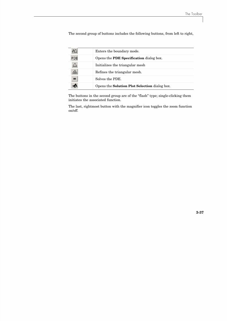
8/21/2019 matlab pde solving.pdf
http://slidepdf.com/reader/full/matlab-pde-solvingpdf 155/290
3-37
The buttons in the second group are of the “flash” type; single-clicking theminitiates the associated function.
The last, rightmost button with the magnifier icon toggles the zoom functionon/off.
Enters the boundary mode.
Opens the PDE Specification dialog box.
Initializes the triangular mesh
Refines the triangular mesh.
Solves the PDE.
Opens the Solution Plot Selection dialog box.
3 The Graphical User Interface

8/21/2019 matlab pde solving.pdf
http://slidepdf.com/reader/full/matlab-pde-solvingpdf 156/290
3-38
4
Th Fi it El t
8/21/2019 matlab pde solving.pdf
http://slidepdf.com/reader/full/matlab-pde-solvingpdf 157/290
The Finite ElementMethod
The core of the PDE Toolbox is a PDE solver that uses the Finite Element Method (FEM) forproblems defined on bounded domains in the plane. The toolbox provides a user-friendly interfacebetween the computing environment of M ATLAB and the technical procedures of the FEM.
The Elliptic Equation (p. 4-2) Mathematical definition anddiscussion of the elliptic equation
The Elliptic System (p. 4-9) Mathematical definition anddiscussion of a system of ellipticequations
The Parabolic Equation (p. 4-12) Mathematical definition anddiscussion of the parabolic equation
The Hyperbolic Equation (p. 4-15) Mathematical definition anddiscussion of the hyperbolic equation
The Eigenvalue Equation (p. 4-16) Mathematical definition anddiscussion of the eigenvalue equation
Nonlinear Equations (p. 4-20) Mathematical definition anddiscussion of nonlinear equations
Adaptive Mesh Refinement (p. 4-25) Description of toolbox meshrefinement
Fast Solution of Poisson’s Equation (p. 4-28) Description of the toolbox solution toPoisson’s equation
References (p. 4-30) Additional information
4 The Finite Element Method
The Elliptic Equation
The basic elliptic equation handled by the toolbox is
8/21/2019 matlab pde solving.pdf
http://slidepdf.com/reader/full/matlab-pde-solvingpdf 158/290
4-2
p q y
in Ω
where Ω is a bounded domain in the plane. c, a, f, and the unknown solution u are complex functions defined on Ω. c can also be a 2-by-2 matrix function onΩ. The boundary conditions specify a combination of u and its normalderivative on the boundary:
• Dirichlet: hu = r on the boundary .•Generalized Neumann: ⋅ (c∇u) + qu = g on .
• Mixed: Only applicable to systems. A combination of Dirichlet andgeneralized Neumann.
is the outward unit normal. g, q, h, and r are functions defined on .
Our nomenclature deviates slightly from the tradition for potential theory,
where a Neumann condition usually refers to the case q = 0 and our Neumannwould be called a mixed condition. In some contexts, the generalized Neumannboundary conditions is also referred to as the Robin boundary conditions. In variational calculus, Dirichlet conditions are also called essential boundaryconditions and restrict the trial space. Neumann conditions are also callednatural conditions and arise as necessary conditions for a solution. The variational form of the PDE Toolbox equation with Neumann conditions isgiven below.
The approximate solution to the elliptic PDE is found in three steps:
1 Describe the geometry of the domain Ω and the boundary conditions. Thiscan be done either interactively using pdetool (see Chapter 3, “TheGraphical User Interface”) or through M-files (see pdegeom and pdebound.)
2 Build a triangular mesh on the domain Ω. The toolbox has mesh generatingand mesh refining facilities. A mesh is described by three matrices of fixed
format that contain information about the mesh points, the boundarysegments, and the triangles.
∇ – c u∇( )⋅ au+ f =
Ω∂
n Ω∂
n Ω∂
The Elliptic Equation
3 Discretize the PDE and the boundary conditions to obtain a linear system Ku = F . The unknown vector u contains the values of the approximatesolution at the mesh points, the matrix K is assembled from the coefficients
8/21/2019 matlab pde solving.pdf
http://slidepdf.com/reader/full/matlab-pde-solvingpdf 159/290
4-3
p ,c, a, h, and q and the right-hand side F contains, essentially, averages of faround each mesh point and contributions from g. Once the matrices K and
F are assembled, you have the entire M ATLAB environment at your disposalto solve the linear system and further process the solution.
More elaborate applications make use of the Finite Element Method (FEM)
specific information returned by the different functions of the toolbox.Therefore we quickly summarize the theory and technique of FEM solvers toenable advanced applications to make full use of the computed quantities.
FEM can be summarized in the following sentence: Project the weak form of the
differential equation onto a finite-dimensional function space. The rest of thissection deals with explaining the above statement.
We start with the weak form of the differential equation. Without restrictingthe generality, we assume generalized Neumann conditions on the wholeboundary, since Dirichlet conditions can be approximated by generalizedNeumann conditions. In the simple case of a unit matrix h, setting g = qr andthen letting yields the Dirichlet condition because division with a verylarge q cancels the normal derivative terms. The actual implementation isdifferent, since the above procedure may create conditioning problems. Themixed boundary condition of the system case requires a more complicatedtreatment, described in the section “The Elliptic System” on page 4-9
Assume that u is a solution of the differential equation. Multiply the equationwith an arbitrary test function v and integrate on Ω:
Integrate by parts (i.e., use Green’s formula) to obtain
The boundary integral can be replaced by the boundary condition:
q ∞→
∇( – c u∇( ) )v⋅ auv xd+ fv xdΩ
!=Ω
!
c u∇( )Ω!
v∇⋅ auv xd n∂Ω!
– + c u∇( )vds⋅ fv xdΩ!
=
c u∇( )Ω
! v∇⋅ auv xd qu – g+( )vds∂Ω
! – + fv xdΩ
!=
4 The Finite Element Method
Replace the original problem with Find u such that
c u∇( )! v∇⋅ auv fv xd – qu – g+( )vds! – +# $' ( =0 v∀
8/21/2019 matlab pde solving.pdf
http://slidepdf.com/reader/full/matlab-pde-solvingpdf 160/290
4-4
This equation is called the variational, or weak, form of the differentialequation. Obviously, any solution of the differential equation is also a solutionof the variational problem. The reverse is true under some restrictions on thedomain and on the coefficient functions. The solution of the variational problemis also called the weak solution of the differential equation.
The solution u and the test functions v belong to some function space V . Thenext step is to choose an N p-dimensional subspace . Project the weak
form of the differential equation onto a finite-dimensional function space simplymeans requesting u and v to lie in rather than V . The solution of the finite
dimensional problem turns out to be the element of that lies closest to the
weak solution when measured in the energy norm (see below). Convergence is
guaranteed if the space tends to V as . Since the differentialoperator is linear, we demand that the variational equation is satisfied for N p
test-functions φi that form a basis, i.e.,
Expand u in the same basis of
and obtain the system of equations
Ω! ∂Ω!# $
V N pV ⊂
V N p
V N p
V N p N P ∞→
∈ V N p
c u∇( )Ω
! φ∇ i⋅ auφi f φidx – qu – g+( )φ ids∂Ω
! – + 0 i, 1 … N p, ,= =
V N p
u x( ) U jφ j x( )
j 1=
N p
"=
c φ j∇( )Ω! φi∇⋅ aφ jφi xd qφ jφi sd
∂Ω!+ +# $' ( j 1=
N p
" U j
= f φi xdΩ
! gφids∂Ω
! i+ 1 … N p, ,=
The Elliptic Equation
Use the following notations:
(Stiffness matrix) K i j, c φ j∇( )Ω! φidx∇⋅=
8/21/2019 matlab pde solving.pdf
http://slidepdf.com/reader/full/matlab-pde-solvingpdf 161/290
4-5
(Mass matrix)
and rewrite the system in the form ( K + M + Q)U = F + G.
K , M , and Q are N p-by- N p matrices, and F and G are N p-vectors. K , M , and F
are produced by assema, while Q, G are produced by assemb. When it is not
necessary to distinguish K , M , and Q or F and G, we collapse the notations to KU = F, which form the output of assempde.
When the problem is self-adjoint and elliptic in the usual mathematical sense,the matrix K + M + Q becomes symmetric and positive definite. Many commonproblems have these characteristics, most notably those that can also beformulated as minimization problems. For the case of a scalar equation, K , M ,and Q are obviously symmetric. If c( x) ≥ δ > 0, a( x) ≥ 0 and q( x) ≥ 0 with q( x) >0 on some part of , then, if U ≠ 0.
U T ( K + M + Q)U is the energy norm. There are many choices of the test-functionspaces. The toolbox uses continuous functions that are linear on each triangleof the mesh. Piecewise linearity guarantees that the integrals defining thestiffness matrix K exist. Projection onto is nothing more than linearinterpolation, and the evaluation of the solution inside a triangle is done justin terms of the nodal values. If the mesh is uniformly refined,approximates the set of smooth functions on Ω.
! M i j, aφ jφidx
Ω!=
Qi j, qφ jφids∂Ω
!=
F i f φidxΩ!
=
Gi gφids∂Ω
!=
Ω∂
U T
K M Q+ +( )U c ∇u2
Ω! au
2 xd qu
2s 0 if U 0≠,>d
∂Ω!+ +=
V N p
V N p
4 The Finite Element Method
A suitable basis for is the set of “tent” or “hat” functions φi. These are linearon each triangle and take the value 0 at all nodes x j except for xi. Requestingφi( xi) = 1 yields the very pleasant property
p
8/21/2019 matlab pde solving.pdf
http://slidepdf.com/reader/full/matlab-pde-solvingpdf 162/290
4-6
I.e., by solving the FEM system we obtain the nodal values of the approximatesolution. Finally note that the basis function φi vanishes on all the triangles
that do not contain the node xi. The immediate consequence is that theintegrals appearing in K i,j , M i,j , Qi,j , F i and Gi only need to be computed on thetriangles that contain the node xi. Secondly, it means that K i,j and M i,j are zerounless xi and x j are vertices of the same triangle and thus K and M are verysparse matrices. Their sparse structure depends on the ordering of the indicesof the mesh points.
The integrals in the FEM matrices are computed by adding the contributionsfrom each triangle to the corresponding entries (i.e., only if the correspondingmesh point is a vertex of the triangle). This process is commonly calledassembling, hence the name of the function assempde.
The assembling routines scan the triangles of the mesh. For each triangle theycompute the so-called local matrices and add their components to the correctpositions in the sparse matrices or vectors. (The local 3-by-3 matrices containthe integrals evaluated only on the current triangle. The coefficients areassumed constant on the triangle and they are evaluated only in the triangle
barycenter.) The integrals are computed using the mid-point rule. Thisapproximation is optimal since it has the same order of accuracy as thepiecewise linear interpolation.
u xi( ) U jφ j xi( )
j 1=
N p
" U i= =
The Elliptic Equation
Consider a triangle given by the nodes P1 , P2 , and P3 as in the following figure.
P1

8/21/2019 matlab pde solving.pdf
http://slidepdf.com/reader/full/matlab-pde-solvingpdf 163/290
4-7
The Local Triangle P1P2P3
Note The local 3-by-3 matrices contain the integrals evaluated only on thecurrent triangle. The coefficients are assumed constant on the triangle and
they are evaluated only in the triangle barycenter.
The simplest computations are for the local mass matrix m:
where Pc is the center of mass of ∆ P1 P2 P3, i.e.,
The contribution to the right side F is just
For the local stiffness matrix we have to evaluate the gradients of the basisfunctions that do not vanish on P1 P2 P3. Since the basis functions are linear onthe triangle P1 P2 P3, the gradients are constants. Denote the basis functions φ1,φ2, and φ3 such that φi( Pi) = 1. If P2 – P3 = [ x1 ,y1]
T then we have that
P
P
2
3
Pc
Pb
x
y1
1
mi j, a Pc( )φ i x( )φ j x( ) xd∇ P1 P2 P3
! a Pc( )area ∆ P1 P2 P3( )
12----------------------------------------- 1 δi j,+( )= =
Pc
P1 P2 P3+ +
3---------------------------------=
f i f Pc( )area ∆ P1 P2 P3( )
3-----------------------------------------=
4 The Finite Element Method
φ1
∇1
2area ∆ P1 P2 P3( )---------------------------------------------
y1
x – 1
=
8/21/2019 matlab pde solving.pdf
http://slidepdf.com/reader/full/matlab-pde-solvingpdf 164/290
4-8
and after integration (taking c as a constant matrix on the triangle)
If two vertices of the triangle lie on the boundary , they contribute to theline integrals associated to the boundary conditions. If the two boundary pointsare P1 and P2, then we have
and
where Pb is the midpoint of P1 P2.
For each triangle the vertices Pm of the local triangle correspond to the indicesim of the mesh points. The contributions of the individual triangle are added tothe matrices such that, e.g.,
This is done by the function assempde. The gradients and the areas of thetriangles are computed by the function pdetrg.
The Dirichlet boundary conditions are treated in a slightly different manner.They are eliminated from the linear system by a procedure that yields asymmetric, reduced system. The function assempde can return matrices K, F,
B, and ud such that the solution is u = Bv + ud where Kv = F . u is an N p-vector,and if the rank of the Dirichlet conditions is rD, then v has N p – rD components.
ki j,1
4area ∆ P1 P2 P3( )--------------------------------------------- y j x – j,[ ]c Pc( )
y1
x – 1
=
Ω∂
Qi j, q Pb( ) P1 P2 –
6------------------------ 1 δi j,+( ) i j,, 1 2,= =
Gi g Pb( ) P1 P2 – 2
------------------------ i, 1 2,= =
K im in, t K im in,← km n, , m n,+ 1 2 3, ,=
The Elliptic System
The Elliptic System
The toolbox can also handle systems of N partial differential equations over thedomain We have the elliptic systemΩ
8/21/2019 matlab pde solving.pdf
http://slidepdf.com/reader/full/matlab-pde-solvingpdf 165/290
4-9
domain . We have the elliptic system
the parabolic system
the hyperbolic system
d - ∇ ⋅ (c ⊗ ∇u) + au = f
and the eigenvalue system
where c is an N -by- N -by-2-by-2 tensor. By the notation ∇ ⋅ (c ⊗ ∇u), we meanthe N-by-1 matrix with (i,1)-component.
The symbols a and d denote N -by- N matrices, and u denotes column vectors oflength N.
The elements cijkl, aij, dij, and f i of c, a, d, and f are stored row-wise in theM ATLAB matrices c, a, d, and f. The case of identity, diagonal, and symmetricmatrices are handled as special cases. For the tensor cijkl this applies both tothe indices i and j, and to the indices k and l.
The PDE Toolbox does not check the ellipticity of the problem, and it is quitepossible to define a system that is not elliptic in the mathematical sense. The
Ω
∇ c u∇⊗( ) au+⋅ – f =
d∂u
∂t------ ∇ c u∇⊗( ) au+⋅ – f =
d∂
2u
∂t2
--------- ∇ c u∇⊗( ) au+⋅ – f =
∂2
u
∂t2
---------
∇ c u∇⊗( ) au+⋅ – λdu=
∂∂ x------
# '
j 1=
N
" ci j 1 1, , ,∂
∂ x------ ∂
∂ x------ci j 1 2, , ,
∂∂ y------ ∂
∂ y------ci j 2 1, , ,
∂∂ x------ ∂
∂ y------ci j 2 2, , ,
∂∂ y------
$ (+ + + u j
4 The Finite Element Method
procedure described above for the scalar case is applied to each component ofthe system, yielding a symmetric positive definite system of equations
whenever the differential system possesses these characteristics.
8/21/2019 matlab pde solving.pdf
http://slidepdf.com/reader/full/matlab-pde-solvingpdf 166/290
4-10
The boundary conditions now in general are mixed, i.e., for each point on theboundary a combination of Dirichlet and generalized Neumann conditions,
By the notation we mean the N-by-1 matrix with (i,1)-component
where the outward normal vector of the boundary is .There are M Dirichlet conditions and the h-matrix is M -by- N , M ≥ 0. The
generalized Neumann condition contains a source h'µ where the Lagrangemultipliers µ are computed such that the Dirichlet conditions become satisfied.In a structural mechanics problem, this term is exactly the reaction forcenecessary to satisfy the kinematic constraints described by the Dirichletconditions.
The rest of this section details the treatment of the Dirichlet conditions andmay be skipped on a first reading.
The PDE Toolbox supports two implementations of Dirichlet conditions. Thesimplest is the “Stiff Spring” model, so named for its interpretation in solidmechanics. See the section “The Elliptic Equation” on page 4-2 for the scalarcase, which is equivalent to a diagonal h-matrix. For the general case, Dirichletconditions
hu = r
are approximated by adding a term
L(h′hu - h′r)
to the equations KU = F , where L is a large number such as 104 times arepresentative size of the elements of K.
hu r=
n c u∇⊗( )⋅ qu+ g h′ µ +=
n c u∇⊗( )=
α ( )ci j 1 1, , ,cos ∂
∂ x------ α ( )cos ci j 1 2, , ,
∂
∂ y------ α ( )sin ci j 2 1, , ,
∂
∂ x------ α ( )sin ci j 2 2, , ,
∂
∂ y------+ + +# $
' (
j 1=
N
" u j
n α ( ) α ( )sin,cos( )=
The Elliptic System
When this number is increased, hu = r will be more accurately satisfied, butthe potential ill-conditioning of the modified equations will become more
serious.

8/21/2019 matlab pde solving.pdf
http://slidepdf.com/reader/full/matlab-pde-solvingpdf 167/290
4-11
The second method is also applicable to general mixed conditions withnondiagonal h, and is free of the ill-conditioning, but is more involvedcomputationally. Assume that there are N p nodes in the triangulation. Thenthe number of unknowns is N p N = N u. When Dirichlet boundary conditions fixsome of the unknowns, the linear system can be correspondingly reduced. Thisis easily done by removing rows and columns when u values are given, but here
we must treat the case when some linear combinations of the components of u are given, hu = r. These are collected into HU = R where H is an M -by- N u matrix and R is an M -vector.
With the reaction force term the system becomes
KU +H ′ µ = F
HU = R
The constraints can be solved for m of the U- variables, the remaining called V ,an N u - m vector. The null space of H is spanned by the columns of B, and
U = BV + ud
makes U satisfy the Dirichlet conditions. A permutation to block-diagonal formexploits the sparsity of H to speed up the following computation to find B in anumerically stable way. µ can be eliminated by premultiplying by B′ since, bythe construction, HB = 0 or B′ H ′ = 0. The reduced system becomes
B′ KBV = B′ F - B′ Kud
which is symmetric and positive definite if K is.
4 The Finite Element Method
The Parabolic Equation
The elliptic solver allows other types of equations to be more or less easilyimplemented Below we show how the parabolic equation can be reduced to
8/21/2019 matlab pde solving.pdf
http://slidepdf.com/reader/full/matlab-pde-solvingpdf 168/290
4-12
implemented. Below we show how the parabolic equation can be reduced tosolving elliptic equations. This is done by the toolbox function parabolic.
Consider the equation
with the initial condition
and boundary conditions of the same kind as for the elliptic equation on .
The heat equation reads
in the presence of distributed heat loss to the surroundings. ρ is the density, C
thermal capacity, k thermal conductivity, h film coefficient, u∞ ambienttemperature, and f heat source.
For time-independent coefficients, the steady state solution of the equation isthe solution to our standard elliptic equation
-∇ ⋅ (c∇u) + au = f
Assuming a triangular mesh on Ω and at any time t ≥ 0, expand the solution tothe PDE (as a function of x) in the Finite Element Method basis:
Plugging the expansion into the PDE, multiplying with a test function φ j,
integrating over Ω, and applying Green’s formula and the boundary conditionsyield
In matrix notation, we have to solve the linear, large and sparse ODE system
d∂u
∂t------ ∇ – c u∇( )⋅ au+ f in Ω=
u x 0,( ) u0 x( ) = x Ω∈
Ω∂
ρC∂u
∂t
------ ∇ – k u∇( )⋅ h u u∞ – ( )+ f =
u x t,( ) U i t( )φι x( )
i
"=
The Parabolic Equation
This method is traditionally called method of lines semidiscretization.
M dU
dt-------- KU + F =
8/21/2019 matlab pde solving.pdf
http://slidepdf.com/reader/full/matlab-pde-solvingpdf 169/290
4-13
Solving the ODE with the initial value
U i(0) = u0( xi)
yields the solution to the PDE at each node xi and time t. Note that K and F arethe stiffness matrix and the right-hand side of the elliptic problem
-∇ ⋅ (c∇u) + au = f in Ω
with the original boundary conditions while M is just the mass matrix of theproblem
-∇ ⋅ (0∇u) + du = 0 in Ω
When the Dirichlet conditions are time dependent, F contains contributionsfrom time derivatives of h and r. These derivatives are evaluated by finitedifferences of the user-specified data.
The ODE system is ill conditioned. Explicit time integrators are forced bystability requirements to very short time steps while implicit solvers can beexpensive since they solve an elliptic problem at every time step. Thenumerical integration of the ODE system is performed by the M ATLAB ODESuite functions, which are efficient for this class of problems. The time step iscontrolled to satisfy a tolerance on the error, and factorizations of coefficientmatrices are performed only when necessary. When coefficients are timedependent, the necessity of reevaluating and refactorizing the matrices eachtime step may still make the solution time consuming, although parabolic
reevaluates only that which varies with time. In certain cases atime-dependent Dirichlet matrix h(t) may cause the error control to fail, evenif the problem is mathematically sound and the solution u(t) is smooth. Thiscan happen because the ODE integrator looks only at the reduced solution v with u = Bv + ud. As h changes, the pivoting scheme employed for numerical
φ jφid xU id t( )
td-----------------d
Ω!
i
" ∇φ jΩ
!# ' c φi∇( )⋅ aφ jφi xd qφ jφi sd
∂Ω! $
( U i t( )+ +
i
"+
f φ jΩ
! xd gφ j∂Ω
! sd j∀+=
4 The Finite Element Method
stability may change the elimination order from one step to the next. Thismeans that B,v and ud all change discontinuously, although u itself does not.

8/21/2019 matlab pde solving.pdf
http://slidepdf.com/reader/full/matlab-pde-solvingpdf 170/290
4-14
The Hyperbolic Equation
The Hyperbolic Equation
Using the same ideas as for the parabolic equation, hyperbolic implementsthe numerical solution of

8/21/2019 matlab pde solving.pdf
http://slidepdf.com/reader/full/matlab-pde-solvingpdf 171/290
4-15
with the initial conditions
and usual boundary conditions. In particular, solutions of the equationutt - c∆u = 0 are waves moving with speed .
Using a given triangulation of Ω, the method of lines yields the second orderODE system
with the initial conditions
after we eliminate the unknowns fixed by Dirichlet boundary conditions. As
before, the stiffness matrix K and the mass matrix M are assembled with theaid of the function assempde from the problems
-∇ ⋅ (c∇u) + au = f and -∇ ⋅ (0∇u) + du = 0
d∂
2u
∂t2
--------- ∇ c∇u( ) au+⋅ – f in Ω=
u x 0,( ) u0= x( ) ∂u∂t------ x 0,( ) v0= x( ) x Ω∈
c
M d2U
dt2
----------- KU + F =
U i 0( ) u0 xi( ),=d
dt------U i 0( ) v0= xi( ) i∀
4 The Finite Element Method
The Eigenvalue Equation
The basic eigenvalue problem handled by the PDE Toolbox is
∇ ( ∇ ) λd
8/21/2019 matlab pde solving.pdf
http://slidepdf.com/reader/full/matlab-pde-solvingpdf 172/290
4-16
-∇ ⋅ (c∇u) + au = λdu
where λ is an unknown complex number. In solid mechanics, this is a problemassociated with wave phenomena describing, e.g., the natural modes of a vibrating membrane. In quantum mechanics λ is the energy level of a boundstate in the potential well a( x).
The numerical solution is found by discretizing the equation and solving theresulting algebraic eigenvalue problem. Let us first consider the discretization.Expand u in the FEM basis, multiply with a basis element, and integrate onthe domain Ω. This yields the generalized eigenvalue equation
KU = λ MU
where the mass matrix corresponds to the right side, i.e.,
The matrices K and M are produced by calling assema for the equations
-∇ ⋅ (c∇u) + au = 0 and -∇ ⋅ (0∇u) + du = 0
Note that in the most common case, when the function d( x) is positive, the massmatrix M is positive definite symmetric. Likewise, when c( x) is positive and wehave Dirichlet boundary conditions, the stiffness matrix K is also positive
definite.The generalized eigenvalue problem, KU = λ MU , is now solved by the Arnoldi
algorithm applied to a shifted and inverted matrix with restarts until alleigenvalues in the user-specified interval have been found.
Let us describe how this is done in more detail. You may want to look at theexample provided in the section “Examples of Eigenvalue Problems” onpage 2-28, where an actual run is reported.
First a shift µ is determined close to where we want to find the eigenvalues.When both K and M are positive definite, it is natural to take µ = 0, and get thesmallest eigenvalues; in other cases take any point in the interval [lb,ub] whereeigenvalues are sought. Subtract µ M from the eigenvalue equation and get
M i j, x( )φ j x( )φ i x( )d xdΩ!=
The Eigenvalue Equation
( K - µ M )U = (λ − µ) MU . Then multiply with the inverse of this shifted matrixand get
.1λ------------U K µ M – ( ) MU
1 – =
8/21/2019 matlab pde solving.pdf
http://slidepdf.com/reader/full/matlab-pde-solvingpdf 173/290
4-17
This is a standard eigenvalue problem AU = θU , with the matrix A = ( K - µ M )-1 M and eigenvalues
where i = 1, . . ., n. The largest eigenvalues θi of the transformed matrix A nowcorrespond to the eigenvalues λi = µ + 1/ θi of the original pencil ( K,M ) closest tothe shift µ.
The Arnoldi algorithm computes an orthonormal basis V where the shifted andinverted operator A is represented by a Hessenberg matrix H ,
AV j=V j H j,j + E j.
(The subscripts mean that V j and E j have j columns and H j,j has j rows andcolumns. When no subscripts are used we deal with vectors and matrices ofsize n.)
Some of the eigenvalues of this Hessenberg matrix H j,j eventually give goodapproximations to the eigenvalues of the original pencil ( K,M ) when the basisgrows in dimension j, and less and less of the eigenvector is hidden in theresidual matrix E j.
The basis V is built one column v j at a time. The first vector v1 is chosen atrandom, as n normally distributed random numbers. In step j, the first j vectorsare already computed and form the n × j matrix V j. The next vector v j + 1 iscomputed by first letting A operate on the newest vector v j, and then makingthe result orthogonal to all the previous vectors.
This is formulated as, h j + 1, jv j + 1 = Av j - V jh j, where the column vector h j consists of the Gram-Schmidt coefficients, and h j + 1, j is the normalization
factor that gives v j + 1 unit length. Put the corresponding relations fromprevious steps in front of this and get
λ µ – µ( )
θi1
λi µ – --------------=
AV j V j H j j, v j 1+ h j 1 j,+ e jT
+=
4 The Finite Element Method
where H j,j is a j × j Hessenberg matrix with the vectors h j as columns. Thesecond term on the right-hand side has nonzeros only in the last column; the
earlier normalization factors show up in the subdiagonal of H j,j.The eigensolution of the small Hessenberg matrix Hj j gives approximations to
8/21/2019 matlab pde solving.pdf
http://slidepdf.com/reader/full/matlab-pde-solvingpdf 174/290
4-18
The eigensolution of the small Hessenberg matrix H j,j gives approximations tosome of the eigenvalues and eigenvectors of the large matrix operator A in thefollowing way. Compute eigenvalues θi and eigenvectors si of H j,j,
H j,jsi = siθi , i = 1, . . . , j
Then yi = V jsiis an approximate eigenvector of A, and its residual is
ri = Ayi - yiθi = AV jsi - V jsiθi = ( AV j - V j H j,j)si = v j+1h j+1 ,jsi,j
This residual has to be small in norm for θi to be a good eigenvalueapproximation. The norm of the residual is ||ri|| = |h j+1,js j,i|, the product ofthe last subdiagonal element of the Hessenberg matrix and the last element ofits eigenvector. It seldom happens that h j+1,j gets particularly small, but aftersufficiently many steps j there are always some eigenvectors si with small lastelements. Note that the long vector V j+1 is of unit norm.
It is not necessary to actually compute the eigenvector approximation yi to getthe norm of the residual; we only need to examine the short vectors si, and flagthose with tiny last components as converged. In a typical case n may be 2000,while j seldom exceeds 50, so all computations that involve only matrices and vectors of size j are much cheaper than those involving vectors of length n.
This eigenvalue computation and test for convergence is done every few steps j, until all approximations to eigenvalues inside the interval [lb,ub] are flagged
as converged. When n is much larger than j, this is done very often, for smallern more seldom. When all eigenvalues inside the interval have converged, orwhen j has reached a prescribed maximum, the converged eigenvectors, ormore appropriately Schur vectors, are computed and put in the front of thebasis V .
After this, the Arnoldi algorithm is restarted with a random vector, if allapproximations inside the interval are flagged as converged, or else with thebest unconverged approximate eigenvector yi. In each step j of this second
Arnoldi run, the vector is made orthogonal to all vectors in V including theconverged Schur vectors from the previous runs. This way, the algorithm isapplied to a projected matrix, and picks up a second copy of any doubleeigenvalue there may be in the interval. If anything in the interval convergesduring this second run, a third is attempted and so on, until no more
The Eigenvalue Equation
approximate eigenvalues θi show up inside. Then the algorithm signalsconvergence. If there are still unconverged approximate eigenvalues after a
prescribed maximum number of steps, the algorithm signals nonconvergenceand reports all solutions it has found.

8/21/2019 matlab pde solving.pdf
http://slidepdf.com/reader/full/matlab-pde-solvingpdf 175/290
4-19
This is a heuristic strategy that has worked well on both symmetric,nonsymmetric, and even defective eigenvalue problems. There is a tinytheoretical chance of missing an eigenvalue, if all the random starting vectorshappen to be orthogonal to its eigenvector. Normally, the algorithm restarts p times, if the maximum multiplicity of an eigenvalue is p. At each restart a newrandom starting direction is introduced.
Note that the shifted and inverted matrix A = ( K - µ M )-1 M is needed only tooperate on a vector v j in the Arnoldi algorithm. This is done by computing anLU factorization,
P( K - µ M )Q = LU
using the sparse M ATLAB command lu ( P and Q are permutations that makethe triangular factors L and U sparse and the factorization numerically stable).
This factorization needs to be done only once, in the beginning, then x = Av j iscomputed as,
x = QU -1 L-1 PMv j
with one sparse matrix vector multiplication, a permutation, sparse forward-and back-substitutions, and a final renumbering.
4 The Finite Element Method
Nonlinear Equations
The low-level functions of the PDE Toolbox are aimed at solving linearequations. Since many interesting computational problems are nonlinear, the
lb l l b l f h f

8/21/2019 matlab pde solving.pdf
http://slidepdf.com/reader/full/matlab-pde-solvingpdf 176/290
4-20
toolbox contains a nonlinear solver built on top of the assempde function.
The basic idea is to use Gauss-Newton iterations to solve the nonlinearequations. Say you are trying to solve the equation
r(u) = –∇ ⋅ (c(u)∇u) + a(u)u - f (u) = 0.
In the FEM setting you solve the weak form of r(u) = 0. Set as usual
then, multiply the equation by an arbitrary test function φi, integrate on thedomain Ω, and use Green’s formula and the boundary conditions to obtain
which has to hold for all indices i.
The residual vector ρ(U ) can be easily computed asρ(U ) = ( K + M + Q)U - ( F + G)
where the matrices K , M , Q and the vectors F and G are produced byassembling the problem
–∇ ⋅ (c(U )∇u) + a(U )u = f (U )
u x( ) U jφ j"=
0 ρ U ( ) c( x U ,( ) φ j x( ) )∇ φi x( )∇⋅ a x U ,( )φ j x( )φ i x( )dx+Ω
!# '
j
"= =
q x U ,( )φ j x( )φ i x( )ds∂Ω
! $ ( U j+
f x U ,( )φ i x( )dxΩ
! – g x U ,( )φ i x( )ds∂Ω
! –
Nonlinear Equations
Assume that you have a guess U (n) of the solution. If U (n) is close enough to theexact solution, an improved approximation U (n + 1) is obtained by solving the
linearized problem
∂ Un( )
( )' (
8/21/2019 matlab pde solving.pdf
http://slidepdf.com/reader/full/matlab-pde-solvingpdf 177/290
4-21
where α is a positive number. (It is not necessary that ρ(U)=0 have a solutioneven if ρ(u) = 0 has. In this case, the Gauss-Newton iteration tends to be theminimizer of the residual, i.e., the solution of minU ||ρ(U)||).
It is well known that for sufficiently small α
||ρ(U (n + 1))|| < ||ρ(U (n))||
and
is called a descent direction for ||ρ(U )||, where ||⋅ || is the l2-norm. Theiteration is
U (n + 1) = U (n) + α pn
where α ≤ 1 is chosen as large as possible such that the step has a reasonabledescent.
The Gauss-Newton method is local, and convergence is assured only when U (0)
is close enough to the solution. In general, the first guess may be outside theregion of convergence. To improve convergence from bad initial guesses, adamping strategy is implemented for choosing α, the Armijo-Goldstein line
search. It chooses the largest damping coefficient α out of the sequence 1, 1/2,1/4, . . . such that the following inequality holds:
||ρ(U (n))|| - ||ρ(U (n)+ α pn)|| ≥ ||ρ(U (n))||
which guarantees a reduction of the residual norm by at least 1 – α /2. Note thateach step of the line-search algorithm requires an evaluation of the residualρ(U (n)+ α pn).
An important point of this strategy is that when U (n) approaches the solution,then and thus the convergence rate increases. If there is a solution to
∂ρ U n( )
( )
∂U -----------------------
# $' ( U
n 1+( )U
n( ) – ( ) α – ρ U
n( )( )=
pn∂ρ U
n( )( )
∂U -----------------------
# $' (
1 –
ρ U n( )
( )=
α
2---
α 1→
4 The Finite Element Method
ρ(U ) = 0, the scheme ultimately recovers the quadratic convergence rate of thestandard Newton iteration.
Closely related to the above problem is the choice of the initial guess U (0). Bydefault, the solver sets U (0) and then assembles the FEM matrices K and F and
8/21/2019 matlab pde solving.pdf
http://slidepdf.com/reader/full/matlab-pde-solvingpdf 178/290
4-22
,computes
U (1) = K -1 F
The damped Gauss-Newton iteration is then started with U (1), which should bea better guess than U (0). If the boundary conditions do not depend on the
solution u, then U (1) satisfies them even if U (0) does not. Furthermore, if theequation is linear, then U (1) is the exact FEM solution and the solver does notenter the Gauss-Newton loop.
There are situations where U (0) = 0 makes no sense or convergence isimpossible.
In some situations you may already have a good approximation and the
nonlinear solver can be started with it, avoiding the slow convergence regime.This idea is used in the adaptive mesh generator. It computes a solution ona mesh, evaluates the error, and may refine certain triangles. The interpolantof is a very good starting guess for the solution on the refined mesh.
In general the exact Jacobian
is not available. Approximation of J n by finite differences in the following wayis expensive but feasible. The ith column of J n can be approximated by
which implies the assembling of the FEM matrices for the triangles containinggrid point i. A very simple approximation to J n, which gives a fixed point
iteration, is also possible as follows. Essentially, for a given U (n
), compute theFEM matrices K and F and set
U (n + 1) = K -1 F
U ˜
U ˜
J n∂ρ U
n( )( )
∂U -----------------------=
1ε--- ρ U (
n( )εφ i ) ρ U
n( )( ) – +( )
Nonlinear Equations
This is equivalent to approximating the Jacobian with the stiffness matrix.Indeed, since ρ(U (n)) = KU (n) - F , putting J n = K yields
U n 1+( )
U n( )
= J n1 –
ρ U n( )
( ) – U n( )
= K 1 –
KU n( )
( – F ) – K 1 – F =
8/21/2019 matlab pde solving.pdf
http://slidepdf.com/reader/full/matlab-pde-solvingpdf 179/290
4-23
In many cases the convergence rate is slow, but the cost of each iteration ischeap.
The nonlinear solver implemented in the PDE Toolbox also provides for acompromise between the two extremes. To compute the derivative of themapping , proceed as follows. The a term has been omitted for clarity,but appears again in the final result below.
The first integral term is nothing more than K i,j.
The second term is “lumped,” i.e., replaced by a diagonal matrix that containsthe row sums. Since Σ j
φ j = 1, the second term is approximated by
which is the ithcomponent of K (c')U , where K (c') is the stiffness matrix
associated with the coefficient rather than c. The same reasoning can be
applied to the derivative of the mapping . Finally note that thederivative of the mapping is exactly
which is the mass matrix associated with the coefficient . Thus the Jacobianof the residual ρ(U ) is approximated by
U KU →
∂ KU ( )i
∂U j-------------------
1ε---
ε 0→lim c U εφ j+( ) φl φidx U l εδ l j,+( )∇∇
Ω!#
'
l
"=
c U ( ) φl φidxU l∇∇Ω
! $ ( –
c U ( ) φ j φidx∇∇Ω! φ j ∂c∂u------ φl φidxU l∇∇
Ω!l
"+=
δi j,
∂c
∂u------ φ
l φ
idxU
l∇∇
Ω!l"
∂c
∂u------
U MU →
U F – →
∂ f ∂u------φiφ jdx
Ω! –
∂ f
∂u------
4 The Finite Element Method
where the differentiation is with respect to u. K and M designate stiffness andmass matrices and their indices designate the coefficients with respect towhich they are assembled At each Gauss Newton iteration the nonlinear
J K c( )
≈ M a f – ′( )
diag K (c ′( )
M a ′( )
)U +( )+ + +
8/21/2019 matlab pde solving.pdf
http://slidepdf.com/reader/full/matlab-pde-solvingpdf 180/290
4-24
which they are assembled. At each Gauss-Newton iteration, the nonlinearsolver assembles the matrices corresponding to the equations
–∇ ⋅ (c∇u) + (a - f') u = 0 and -∇ ⋅ (c'∇u) + a'u = 0
and then produces the approximate Jacobian. The differentiations of thecoefficients are done numerically.
In the general setting of elliptic systems, the boundary conditions areappended to the stiffness matrix to form the full linear system:
where the coefficients of and may depend on the solution . The “lumped”
approach approximates the derivative mapping of the residual by
The nonlinearities of the boundary conditions and the dependencies of thecoefficients on the derivatives of are not properly linearized by this scheme.When such nonlinearities are strong, the scheme reduces to the fix-point
iteration and may converge slowly or not at all. When the boundary conditionsare linear, they do not affect the convergence properties of the iterationschemes. In the Neumann case they are invisible ( H is an empty matrix) andin the Dirichlet case they merely state that the residual is zero on thecorresponding boundary points.
K ˜ U ˜ K H ′
H 0U
µ
F
R F ˜= = =
K ˜ F ˜ U ˜
J H ′
H 0
U ˜
Adaptive Mesh Refinement
Adaptive Mesh Refinement
The toolbox has a function for global, uniform mesh refinement. It divides eachtriangle into four similar triangles by creating new corners at the midsides,adjusting for curved boundaries You can assess the accuracy of the numerical
8/21/2019 matlab pde solving.pdf
http://slidepdf.com/reader/full/matlab-pde-solvingpdf 181/290
4-25
adjusting for curved boundaries. You can assess the accuracy of the numericalsolution by comparing results from a sequence of successively refined meshes.If the solution is smooth enough, more accurate results may be obtained byextrapolation.
The solutions of the toolbox equation often have geometric features like
localized strong gradients. An example of engineering importance in elasticityis the stress concentration occurring at reentrant corners such as the M ATLAB favorite, the L-shaped membrane. Then it is more economical to refine themesh selectively, i.e., only where it is needed. When the selection is based onestimates of errors in the computed solutions, a posteriori estimates, we speakof adaptive mesh refinement. See adaptmesh for an example of thecomputational savings where global refinement needs more than 6000elements to compete with an adaptively refined mesh of 500 elements.
The adaptive refinement generates a sequence of solutions on successivelyfiner meshes, at each stage selecting and refining those elements that are judged to contribute most to the error. The process is terminated when themaximum number of elements is exceeded or when each triangle contributesless than a preset tolerance. You need to provide an initial mesh, and chooseselection and termination criteria parameters. The initial mesh can beproduced by the initmesh function. The three components of the algorithm arethe error indicator function, which computes an estimate of the element error
contribution, the mesh refiner, which selects and subdivides elements, and thetermination criteria.
The Error Indicator FunctionThe adaption is a feedback process. As such, it is easily applied to a largerrange of problems than those for which its design was tailored. You wantestimates, selection criteria, etc., to be optimal in the sense of giving the mostaccurate solution at fixed cost or lowest computational effort for a givenaccuracy. Such results have been proved only for model problems, butgenerally, the equidistribution heuristic has been found near optimal. Elementsizes should be chosen such that each element contributes the same to theerror. The theory of adaptive schemes makes use of a priori bounds forsolutions in terms of the source function f . For nonelliptic problems such a
4 The Finite Element Method
bound may not exist, while the refinement scheme is still well defined and hasbeen found to work well.
The error indicator function used in the toolbox is an element-wise estimate ofthe contribution, based on the work of C. Johnson et al. [5], [6]. For Poisson's

8/21/2019 matlab pde solving.pdf
http://slidepdf.com/reader/full/matlab-pde-solvingpdf 182/290
4-26
equation –∆u = f on Ω, the following error estimate for the FEM-solution uh holds in the L2-norm || ⋅ ||:
|| ∇(u - uh) || ≤ α || hf || + β Dh(uh)
where h = h( x) is the local mesh size, and
The braced quantity is the jump in normal derivative of v across edge τ, hr isthe length of edge τ, and the sum runs over Ei, the set of all interior edges ofthe triangulation. The coefficients α and β are independent of thetriangulation. This bound is turned into an element-wise error indicator
function E( K ) for element K by summing the contributions from its edges. Thefinal form for the toolbox equation
–∇ ⋅ (c∇u) + au = f
becomes
where nτ is the unit normal of edge τ and the braced term is the jump in fluxacross the element edge. The L2 norm is computed over the element K. Thiserror indicator is computed by the pdejmps function.
The Mesh RefinerThe PDE Toolbox is geared to elliptic problems. For reasons of accuracy and
ill-conditioning, they require the elements not to deviate too much from beingequilateral. Thus, even at essentially one-dimensional solution features, suchas boundary layers, the refinement technique must guarantee reasonablyshaped triangles.
Dh v( ) hτ2
∂v ∂nτ ⁄ [ ]2
τ E1∈
"# $% &' ( 1 2 ⁄
=
E K ( ) α h f ( au ) – K = β12--- hτ
2nr c uh∇⋅[ ]
2
τ ∂ K ∈
"# $% &' ( 1 2 ⁄
+
Adaptive Mesh Refinement
When an element is refined, new nodes appear on its midsides, and if theneighbor triangle is not refined in a similar way, it is said to have hanging
nodes. The final triangulation must have no hanging nodes, and they areremoved by splitting neighbor triangles. To avoid further deterioration oftriangle quality in successive generations, the “longest edge bisection” scheme
8/21/2019 matlab pde solving.pdf
http://slidepdf.com/reader/full/matlab-pde-solvingpdf 183/290
4-27
triangle quality in successive generations, the longest edge bisection schemeRosenberg-Stenger [8] is used, in which the longest side of a triangle is alwayssplit, whenever any of the sides have hanging nodes. This guarantees that noangle is ever smaller than half the smallest angle of the original triangulation.
Two selection criteria can be used. One, pdeadworst, refines all elements with value of the error indicator larger than half the worst of any element. Theother, pdeadgsc, refines all elements with an indicator value exceeding auser-defined dimensionless tolerance. The comparison with the tolerance isproperly scaled with respect to domain and solution size, etc.
The Termination CriteriaFor smooth solutions, error equidistribution can be achieved by the pdeadgsc selection if the maximum number of elements is large enough. The pdeadworst
adaption only terminates when the maximum number of elements has beenexceeded. This mode is natural when the solution exhibits singularities. Theerror indicator of the elements next to the singularity may never vanish,regardless of element size, and equidistribution is too much to hope for.
4 The Finite Element Method
Fast Solution of Poisson’s Equation
While the general strategy of the PDE Toolbox is to use the MATLAB built-insolvers for sparse systems, there are situations where faster solutionalgorithms are available. One such example is found when solving Poisson’s
8/21/2019 matlab pde solving.pdf
http://slidepdf.com/reader/full/matlab-pde-solvingpdf 184/290
4-28
algorithms are available. One such example is found when solving Poisson sequation
-∆u = f in Ω
with Dirichlet boundary conditions, where Ω is a rectangle.
For the fast solution algorithms to work, the mesh on the rectangle must be aregular mesh. In this context it means that the first side of the rectangle isdivided into N 1 segments of length h1, the second into N 2 segments of lengthh2, and ( N 1 + 1 ) b y ( N 2 + 1) points are introduced on the regular grid thusdefined. The triangles are all congruent with sides h1, h2 and a right angle inbetween.
The Dirichlet boundary conditions are eliminated in the usual way, and theresulting problem for the interior nodes is Kv = F . If the interior nodes are
numbered from left to right, and then from bottom to top, the K matrix is blocktridiagonal. The N 2 - 1 diagonal blocks, here called T , are themselvestridiagonal ( N 1 - 1 ) b y ( N 1 - 1) matrices, with 2(h1 / h2 + h2 / h1) on the diagonaland -h2 / h1 on the subdiagonals. The subdiagonal blocks, here called I , are -h1 / h2
times the unit N 1 - 1 matrix.
The key to the solution of the problem Kv = F is that the problem Tw = f ispossible to solve using the discrete sine transform. Let S be the( N
1
- 1 ) b y ( N 1
- 1) matrix with Sij
= sin(πij / N 1
). Then S-1TS = Λ, where Λ is adiagonal matrix with diagonal entries 2(h1 / h2 + h2 / h1) - 2h2 / h1 cos(πi / N 1).w = SΛ-1 S-1 f , but multiplying with S is nothing more than taking the discretesine transform, and multiplying with S-1 is the same as taking the inversediscrete sine transform. The discrete sine transform can be efficientlycalculated using the fast Fourier transform on a sequence of length 2 N 1.
Fast Solution of Poisson’s Equation
Solving Tw = f using the discrete sine transform would not be an advantage initself, since the system is tridiagonal and should be solved as such. However,
for the full system Kv = F , a transformation of the blocks in K turns it into N 1 - 1 decoupled tridiagonal systems of size N 2 - 1. Thus, a solution algorithmwould look like
8/21/2019 matlab pde solving.pdf
http://slidepdf.com/reader/full/matlab-pde-solvingpdf 185/290
4-29
1 Divide F into N 2 - 1 blocks of length N 1 - 1, and perform an inverse discretesine transform on each block.
2 Reorder the elements and solve N 1 - 1 tridiagonal systems of size N 2 - 1, with
2(h1 / h2 + h2 / h1) - 2h2 / h1 cos(πi / N 1) on the diagonal, and -h1 / h2 on thesubdiagonals.
3 Reverse the reordering, and perform N 2 - 1 discrete sine transforms on theblocks of length N 1 - 1.
When using a fast solver such as this one, time and memory are also savedsince the matrix K in fact never has to be assembled. A drawback is that since
the mesh has to be regular, it is impossible to do adaptive mesh refinement.The fast elliptic solver for Poisson’s equation is implemented in poisolv. Thediscrete sine transform and the inverse discrete sine transform are computedby dst and idst, respectively.
4 The Finite Element Method
References
[1] Bank, Randolph E., PLTMG: A Software Package for Solving Elliptic Partial Differential Equations, User's Guide 6.0, Society for Industrial and Applied Mathematics, Philadelphia, PA, 1990.
8/21/2019 matlab pde solving.pdf
http://slidepdf.com/reader/full/matlab-pde-solvingpdf 186/290
4-30
pp , p , ,
[2] Dahlquist, Germund, and Björk, Åke, Numerical Methods, 2nd edition,1995, in print.
[3] Golub, Gene H., and Charles F. Van Loan, Matrix Computations, 2ndedition, John Hopkins University Press, Baltimore, MD, 1989.
[4] George, P.L., Automatic Mesh Generation—Application to Finite Element
Methods, Wiley, 1991.
[5] Johnson, C., Numerical Solution of Partial Differential Equations by the
Finite Element Method, Studentlitteratur, Lund, Sweden, 1987.
[6] Johnson, C., and Eriksson, K., Adaptive Finite Element Methods for
Parabolic Problems I: A Linear Model Problem, SIAM J. Numer. Anal, 28,
(1991), pp. 43–77.[7] Saad, Yousef, Variations on Arnoldi's Method for Computing Eigenelements
of Large Unsymmetric Matrices, Linear Algebra and its Applications, Vol 34,1980, pp. 269–295.
[8] Rosenberg, I.G., and F. Stenger, A lower bound on the angles of triangles
constructed by bisecting the longest side, Math. Comp. 29 (1975), pp 390–395.
[9] Strang, Gilbert, Introduction to Applied Mathematics, Wellesley-Cambridge
Press, Cambridge, MA, 1986.[10] Strang, Gilbert, and Fix, George, An Analysis of the Finite Element
Method, Prentice-Hall Englewoood Cliffs, N.J., USA, 1973.
5
Function Reference
8/21/2019 matlab pde solving.pdf
http://slidepdf.com/reader/full/matlab-pde-solvingpdf 187/290
This chapter contains detailed descriptions of most of the functions in the Partial Differential
Equation (PDE) Toolbox. Some of the functions that are used by the graphical user interface (GUI)function pdetool are not listed in this chapter because they are not used directly — they are calledfrom pdetool.
Functions — By Category (p. 5-2) Lists the functions in category tables.
Functions — Alphabetical List (p. 5-7) Lists the functions in alphabetical order.
5 Function Reference
Functions — By Category
The following topics group PDE functions by category:
• “PDE Algorithms” on page 5-3
8/21/2019 matlab pde solving.pdf
http://slidepdf.com/reader/full/matlab-pde-solvingpdf 188/290
5-2
• “User Interface Algorithms” on page 5-3
• “Geometry Algorithms” on page 5-3
• “Plot Functions” on page 5-5
• “Utility Algorithms” on page 5-5
• “User Defined Algorithms” on page 5-6• “Demonstration Programs” on page 5-6
Functions — By Category
PDE Algorithms
Function Purposeadaptmesh Adaptive mesh generation and PDE solution.
assema Assemble area integral contributions

8/21/2019 matlab pde solving.pdf
http://slidepdf.com/reader/full/matlab-pde-solvingpdf 189/290
5-3
User Interface Algorithms
Geometry Algorithms
assema Assemble area integral contributions.
assemb Assemble boundary condition contributions
assempde Assemble the stiffness matrix and right-hand side of aPDE problem.
hyperbolic Solve hyperbolic PDE problem.parabolic Solve parabolic PDE problem.
pdeeig Solve eigenvalue PDE problem.
pdenonlin Solve nonlinear PDE problem.
poisolv Fast solution of Poisson’s equation on a rectangulargrid.
Function Purpose
pdecirc Draw circle.
pdeellip Draw ellipse.
pdemdlcv
Convert PDE Toolbox 1.0 Model M-filespdepoly Draw polygon.
pderect Draw rectangle.
pdetool PDE Toolbox graphical user interface (GUI).
Function Purpose
csgchk Check validity of Geometry Description Matrix.
csgdel Delete borders between minimal regions.
5 Function Reference
decsg Decompose Constructive Solid Geometry into minimalregions.
initmesh Create initial triangular mesh.
Function Purpose
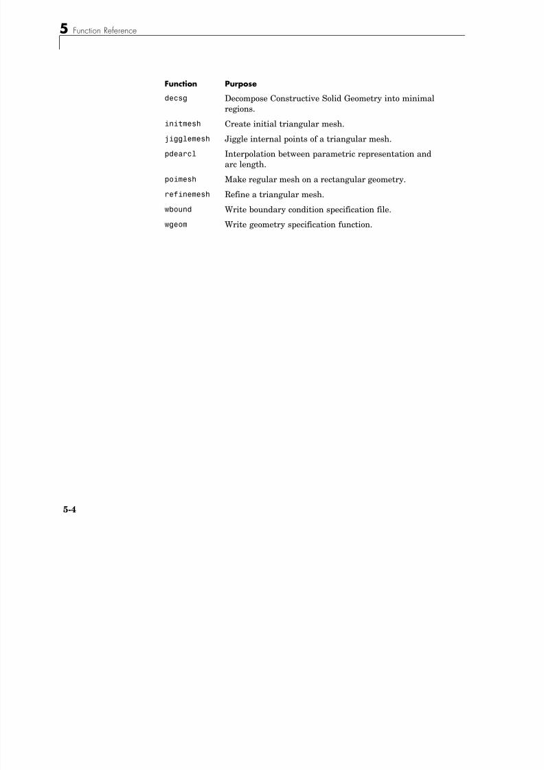
8/21/2019 matlab pde solving.pdf
http://slidepdf.com/reader/full/matlab-pde-solvingpdf 190/290
5-4
g
jigglemesh Jiggle internal points of a triangular mesh.
pdearcl Interpolation between parametric representation andarc length.
poimesh Make regular mesh on a rectangular geometry.refinemesh Refine a triangular mesh.
wbound Write boundary condition specification file.
wgeom Write geometry specification function.
Functions — By Category
Plot Functions
Function Purposepdecont Shorthand command for contour plot.
pdegplot Plot a PDE geometry
8/21/2019 matlab pde solving.pdf
http://slidepdf.com/reader/full/matlab-pde-solvingpdf 191/290
5-5
Utility Algorithms
pdegplot Plot a PDE geometry.
pdemesh Plot a PDE triangular mesh.
pdeplot Generic PDE Toolbox plot function.
pdesurf Shorthand command for surface plot.
Function Purpose
dst Discrete sine transform.
idst Inverse discrete sine transform.
pdeadgsc Select triangles using a relative tolerance criterion.pdeadworst Select triangles relative to the worst value.
pdecgrad The flux of a PDE solution.
pdeent Indices of triangles neighboring a given set of triangles.
pdegrad The gradient of a PDE solution.
pdeintrp Interpolate from node data to triangle midpoint data.
pdejmps Error estimates for adaption.
pdeprtni Interpolate from triangle midpoint data to node data.
pdesde Indices of edges in a set of subdomains.
pdesdp Indices of points in a set of subdomains.
pdesdt Indices of triangles in a set of subdomains.
pdesmech Calculate structural mechanics tensor functions.pdetrg Triangle geometry data.
pdetriq Triangle quality measure.
5 Function Reference
poiasma Boundary point matrix contributions for fast solvers ofPoisson’s equation.
poicalc Fast solver for Poisson’s equation on a
Function Purpose
8/21/2019 matlab pde solving.pdf
http://slidepdf.com/reader/full/matlab-pde-solvingpdf 192/290
5-6
User Defined Algorithms
Demonstration Programs
rectangular grid.
poiindex Indices of points in canonical ordering for arectangular grid.
sptarn Solve generalized sparse eigenvalue problem.
tri2grid Interpolate from PDE triangular mesh to arectangular grid.
Function Purpose
pdebound Boundary M-file.
pdegeom Geometry M-file.
Function Purpose
pdedemo1 Exact solution of Poisson’s equation on unit disk.
pdedemo2 Solve Helmholtz’s equation and study the reflectedwaves.
pdedemo3 Solve a minimal surface problem.
pdedemo4 Solve PDE problem using subdomain decomposition.
pdedemo5 Solve a parabolic PDE (the heat equation).
pdedemo6 Solve a hyperbolic PDE (the wave equation).
pdedemo7 Adaptive solution with point source.pdedemo8 Solve Poisson’s equation on rectangular grid.
Functions — Alphabetical List
Functions — Alphabetical List 5
adaptmesh . . . . . . . . . . . . . . . . . . . . . . . . . . . . . . . . . . . . . . . . . . . . . . . . . . . 5-9assema . . . . . . . . . . . . . . . . . . . . . . . . . . . . . . . . . . . . . . . . . . . . . . . . . . . . . 5-14assemb . . . . . . . . . . . . . . . . . . . . . . . . . . . . . . . . . . . . . . . . . . . . . . . . . . . . . 5-15
8/21/2019 matlab pde solving.pdf
http://slidepdf.com/reader/full/matlab-pde-solvingpdf 193/290
5-7
assempde . . . . . . . . . . . . . . . . . . . . . . . . . . . . . . . . . . . . . . . . . . . . . . . . . . . 5-19csgchk . . . . . . . . . . . . . . . . . . . . . . . . . . . . . . . . . . . . . . . . . . . . . . . . . . . . . . 5-29csgdel . . . . . . . . . . . . . . . . . . . . . . . . . . . . . . . . . . . . . . . . . . . . . . . . . . . . . . 5-30decsg . . . . . . . . . . . . . . . . . . . . . . . . . . . . . . . . . . . . . . . . . . . . . . . . . . . . . . . 5-31dst, idst . . . . . . . . . . . . . . . . . . . . . . . . . . . . . . . . . . . . . . . . . . . . . . . . . . . . . 5-36hyperbolic . . . . . . . . . . . . . . . . . . . . . . . . . . . . . . . . . . . . . . . . . . . . . . . . . . . 5-37initmesh . . . . . . . . . . . . . . . . . . . . . . . . . . . . . . . . . . . . . . . . . . . . . . . . . . . . 5-40 jigglemesh . . . . . . . . . . . . . . . . . . . . . . . . . . . . . . . . . . . . . . . . . . . . . . . . . . 5-44parabolic . . . . . . . . . . . . . . . . . . . . . . . . . . . . . . . . . . . . . . . . . . . . . . . . . . . . 5-45pdeadgsc . . . . . . . . . . . . . . . . . . . . . . . . . . . . . . . . . . . . . . . . . . . . . . . . . . . . 5-47pdeadworst . . . . . . . . . . . . . . . . . . . . . . . . . . . . . . . . . . . . . . . . . . . . . . . . . . 5-48pdearcl . . . . . . . . . . . . . . . . . . . . . . . . . . . . . . . . . . . . . . . . . . . . . . . . . . . . . 5-49
pdebound . . . . . . . . . . . . . . . . . . . . . . . . . . . . . . . . . . . . . . . . . . . . . . . . . . . 5-50pdecgrad . . . . . . . . . . . . . . . . . . . . . . . . . . . . . . . . . . . . . . . . . . . . . . . . . . . . 5-52pdecirc . . . . . . . . . . . . . . . . . . . . . . . . . . . . . . . . . . . . . . . . . . . . . . . . . . . . . 5-53pdecont . . . . . . . . . . . . . . . . . . . . . . . . . . . . . . . . . . . . . . . . . . . . . . . . . . . . . 5-54pdeeig . . . . . . . . . . . . . . . . . . . . . . . . . . . . . . . . . . . . . . . . . . . . . . . . . . . . . . 5-55pdeellip . . . . . . . . . . . . . . . . . . . . . . . . . . . . . . . . . . . . . . . . . . . . . . . . . . . . . 5-58pdeent . . . . . . . . . . . . . . . . . . . . . . . . . . . . . . . . . . . . . . . . . . . . . . . . . . . . . . 5-59pdegeom . . . . . . . . . . . . . . . . . . . . . . . . . . . . . . . . . . . . . . . . . . . . . . . . . . . . 5-60pdegplot . . . . . . . . . . . . . . . . . . . . . . . . . . . . . . . . . . . . . . . . . . . . . . . . . . . . 5-63pdegrad . . . . . . . . . . . . . . . . . . . . . . . . . . . . . . . . . . . . . . . . . . . . . . . . . . . . . 5-64pdeintrp . . . . . . . . . . . . . . . . . . . . . . . . . . . . . . . . . . . . . . . . . . . . . . . . . . . . 5-65pdejmps . . . . . . . . . . . . . . . . . . . . . . . . . . . . . . . . . . . . . . . . . . . . . . . . . . . . 5-66pdemdlcv . . . . . . . . . . . . . . . . . . . . . . . . . . . . . . . . . . . . . . . . . . . . . . . . . . . 5-67pdemesh . . . . . . . . . . . . . . . . . . . . . . . . . . . . . . . . . . . . . . . . . . . . . . . . . . . . 5-68pdenonlin . . . . . . . . . . . . . . . . . . . . . . . . . . . . . . . . . . . . . . . . . . . . . . . . . . . 5-69
pdeplot . . . . . . . . . . . . . . . . . . . . . . . . . . . . . . . . . . . . . . . . . . . . . . . . . . . . . 5-72pdepoly . . . . . . . . . . . . . . . . . . . . . . . . . . . . . . . . . . . . . . . . . . . . . . . . . . . . . 5-74pdeprtni . . . . . . . . . . . . . . . . . . . . . . . . . . . . . . . . . . . . . . . . . . . . . . . . . . . . 5-75pderect . . . . . . . . . . . . . . . . . . . . . . . . . . . . . . . . . . . . . . . . . . . . . . . . . . . . . 5-76pdesdp, pdesde, pdesdt . . . . . . . . . . . . . . . . . . . . . . . . . . . . . . . . . . . . . . . . 5-77
5
pdesmech . . . . . . . . . . . . . . . . . . . . . . . . . . . . . . . . . . . . . . . . . . . . . . . . . . . 5-78pdesurf . . . . . . . . . . . . . . . . . . . . . . . . . . . . . . . . . . . . . . . . . . . . . . . . . . . . . 5-80
pdetool . . . . . . . . . . . . . . . . . . . . . . . . . . . . . . . . . . . . . . . . . . . . . . . . . . . . . 5-81pdetrg . . . . . . . . . . . . . . . . . . . . . . . . . . . . . . . . . . . . . . . . . . . . . . . . . . . . . . 5-86pdetriq . . . . . . . . . . . . . . . . . . . . . . . . . . . . . . . . . . . . . . . . . . . . . . . . . . . . . 5-87
8/21/2019 matlab pde solving.pdf
http://slidepdf.com/reader/full/matlab-pde-solvingpdf 194/290
5-8
poiasma . . . . . . . . . . . . . . . . . . . . . . . . . . . . . . . . . . . . . . . . . . . . . . . . . . . . 5-88poicalc . . . . . . . . . . . . . . . . . . . . . . . . . . . . . . . . . . . . . . . . . . . . . . . . . . . . . . 5-89poiindex . . . . . . . . . . . . . . . . . . . . . . . . . . . . . . . . . . . . . . . . . . . . . . . . . . . . 5-90poimesh . . . . . . . . . . . . . . . . . . . . . . . . . . . . . . . . . . . . . . . . . . . . . . . . . . . . 5-91poisolv . . . . . . . . . . . . . . . . . . . . . . . . . . . . . . . . . . . . . . . . . . . . . . . . . . . . . . 5-92refinemesh . . . . . . . . . . . . . . . . . . . . . . . . . . . . . . . . . . . . . . . . . . . . . . . . . . 5-93sptarn . . . . . . . . . . . . . . . . . . . . . . . . . . . . . . . . . . . . . . . . . . . . . . . . . . . . . . 5-95tri2grid . . . . . . . . . . . . . . . . . . . . . . . . . . . . . . . . . . . . . . . . . . . . . . . . . . . . . 5-98wbound . . . . . . . . . . . . . . . . . . . . . . . . . . . . . . . . . . . . . . . . . . . . . . . . . . . . . 5-99wgeom . . . . . . . . . . . . . . . . . . . . . . . . . . . . . . . . . . . . . . . . . . . . . . . . . . . . . 5-100
5adaptmeshPurpose Adaptive mesh generation and PDE solution
Syntax [u,p,e,t]=adaptmesh(g,b,c,a,f)[u,p,e,t]=adaptmesh(g,b,c,a,f,'PropertyName',PropertyValue,)
D i ti d h( b f 'P ' P l )

8/21/2019 matlab pde solving.pdf
http://slidepdf.com/reader/full/matlab-pde-solvingpdf 195/290
5-9
Description [u,p,e,t]=adaptmesh(g,b,c,a,f,'PropertyName',PropertyValue,)
performs adaptive mesh generation and PDE solution. Optional arguments aregiven as property name/property value pairs.
The function produces a solution u to the elliptic scalar PDE problem
–∇ ⋅ (c∇u) + au = f on Ω or the elliptic system PDE problem
–∇ ⋅ (c ⊗ ∇u) + au = f on Ω
with the problem geometry and boundary conditions given by g and b. Themesh is described by the p, e, and t.
The solution u is represented as the solution vector u. For details on the
representation of the solution vector, see assempde on page 5-19.The algorithm works by solving a sequence of PDE problems using refinedtriangular meshes. The first triangular mesh generation is obtained either asan optional argument to adaptmesh or by a call to initmesh without options.The following generations of triangular meshes are obtained by solving thePDE problem, computing an error estimate, selecting a set of triangles basedon the error estimate, and then finally refining these triangles. The solution to
the PDE problem is then recomputed. The loop continues until no triangles areselected by the triangle selection method, or until the maximum number oftriangles is attained, or until the maximum number of triangle generations hasbeen generated.
g describes the decomposed geometry of the PDE problem. g can either be aDecomposed Geometry matrix or the name of a Geometry M-file. The formatsof the Decomposed Geometry matrix and Geometry M-file are described in theentries on decsg and pdegeom, respectively.
b describes the boundary conditions of the PDE problem. b can be either aBoundary Condition matrix or the name of a Boundary M-file. The formats ofthe Boundary Condition matrix and Boundary M-file are described in theentries on assemb and pdebound, respectively.
5
The adapted triangular mesh of the PDE problem is given by the mesh data p,e, and t. For details on the mesh data representation, see initmesh on
page 5-40.The coefficients c, a, and f of the PDE problem can be given in a wide varietyof ways. In the context of adaptmesh the coefficients can depend on u if the
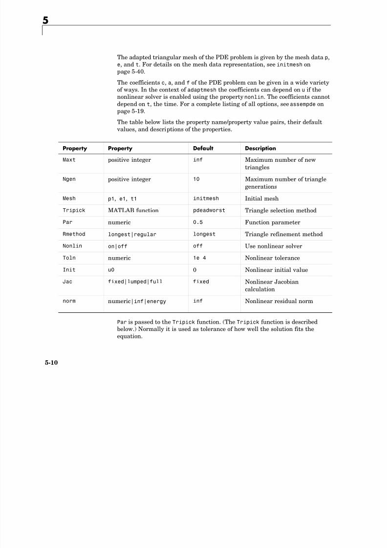
8/21/2019 matlab pde solving.pdf
http://slidepdf.com/reader/full/matlab-pde-solvingpdf 196/290
5-10
nonlinear solver is enabled using the property nonlin. The coefficients cannotdepend on t, the time. For a complete listing of all options, see assempde onpage 5-19.
The table below lists the property name/property value pairs, their default
values, and descriptions of the properties.
Par is passed to the Tripick function. (The Tripick function is describedbelow.) Normally it is used as tolerance of how well the solution fits theequation.
Property Property Default Description
Maxt positive integer inf Maximum number of newtriangles
Ngen positive integer 10 Maximum number of triangle
generationsMesh p1, e1, t1 initmesh Initial mesh
Tripick MATLAB function pdeadworst Triangle selection method
Par numeric 0.5 Function parameter
Rmethod longest|regular longest Triangle refinement method
Nonlin on|off off Use nonlinear solverToln numeric 1e 4 Nonlinear tolerance
Init u0 0 Nonlinear initial value
Jac fixed|lumped|full fixed Nonlinear Jacobiancalculation
norm numeric|inf|energy inf Nonlinear residual norm
No more than Ngen successive refinements are attempted. Refinement is alsostopped when the number of triangles in the mesh exceeds Maxt.
p1, e1, and t1 are the input mesh data. This triangular mesh is used as startingmesh for the adaptive algorithm. For details on the mesh data representation,see initmesh on page 5-40. If no initial mesh is provided, the result of a call to
i h i i d h i i i l h
8/21/2019 matlab pde solving.pdf
http://slidepdf.com/reader/full/matlab-pde-solvingpdf 197/290
5-11
initmesh with no options is used as the initial mesh.
The triangle selection method, Tripick, is a user-definable triangle selectionmethod. Given the error estimate computed by the function pdejmps, thetriangle selection method selects the triangles to be refined in the next triangle
generation. The function is called using the arguments p, t, cc, aa, ff, u, errf,and par. p and t represent the current generation of triangles, cc, aa, and ff are the current coefficients for the PDE problem, expanded to trianglemidpoints, u is the current solution, errf is the computed error estimate, andpar, the function parameter, given to adaptmesh as optional argument. Thematrices cc, aa, ff, and errf all have N t columns, where N t is the currentnumber of triangles. The number of rows in cc, aa, and ff are exactly the sameas the input arguments c, a, and f. errf has one row for each equation in the
system. There are two standard triangle selection methods in the toolbox —pdeadworst and pdeadgsc. pdeadworst selects triangles where errf exceeds afraction (default: 0.5) of the the worst value, and pdeadgsc selects trianglesusing a relative tolerance criterion.
The refinement method is either longest or regular. For details on therefinement method, see refinemesh.
The adaptive algorithm can also solve nonlinear PDE problems. For nonlinear
PDE problems, the Nonlin parameter must be set to on. The nonlineartolerance Toln, nonlinear initial value u0, nonlinear Jacobian calculation Jac,and nonlinear residual norm Norm are passed to the nonlinear solverpdenonlin. For details on the nonlinear solver, see pdenonlin .
5
Examples Solve the Laplace equation over a circle sector, with Dirichlet boundaryconditions u = cos(2/3atan2( y,x)) along the arc, and u = 0 along the straight
lines, and compare to the exact solution. We refine the triangles using theworst error criterion until we obtain a mesh with at least 500 triangles:
[u,p,e,t]=adaptmesh('cirsg','cirsb',1,0,0,'maxt',500,...
' i i k' ' d d ' ' ' i f

8/21/2019 matlab pde solving.pdf
http://slidepdf.com/reader/full/matlab-pde-solvingpdf 198/290
5-12
'tripick','pdeadworst','ngen',inf);
x=p(1,:); y=p(2,:);
exact=((x.^2+y.^2).(1/3).*cos(2/3*atan2(y,x)))';
max(abs(u exact))
ans =
0.0058
size(t,2)
ans =
534
pdemesh(p,e,t)
The maximum absolute error is 0.0058, with 534 triangles. We test how manyrefinements we have to use with a uniform triangle net:
[p,e,t]=initmesh('cirsg');
[p,e,t]=refinemesh('cirsg',p,e,t);
u=assempde('cirsb',p,e,t,1,0,0);
x=p(1,:); y=p(2,:);
exact=((x.^2+y.^2).^(1/3).*cos(2/3*atan2(y,x)))';max(abs(u exact))
ans =
0.0085
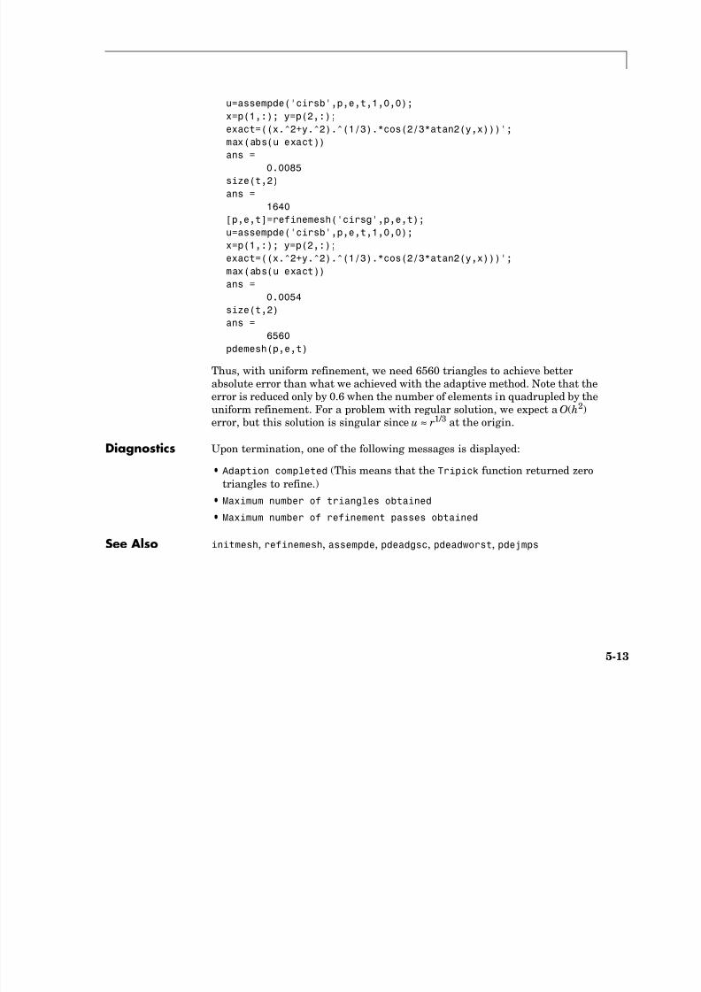
8/21/2019 matlab pde solving.pdf
http://slidepdf.com/reader/full/matlab-pde-solvingpdf 199/290
5-13
size(t,2)
ans =
1640
[p,e,t]=refinemesh('cirsg',p,e,t);
u=assempde('cirsb',p,e,t,1,0,0);x=p(1,:); y=p(2,:);
exact=((x.^2+y.^2).^(1/3).*cos(2/3*atan2(y,x)))';
max(abs(u exact))
ans =
0.0054
size(t,2)
ans =
6560
pdemesh(p,e,t)
Thus, with uniform refinement, we need 6560 triangles to achieve betterabsolute error than what we achieved with the adaptive method. Note that theerror is reduced only by 0.6 when the number of elements in quadrupled by theuniform refinement. For a problem with regular solution, we expect a O(h2)error, but this solution is singular since u ≈ r1/3 at the origin.
Diagnostics Upon termination, one of the following messages is displayed:
• Adaption completed (This means that the Tripick function returned zerotriangles to refine.)
• Maximum number of triangles obtained
• Maximum number of refinement passes obtained
See Also initmesh, refinemesh, assempde, pdeadgsc, pdeadworst, pdejmps
5
5assemaPurpose Assemble area integral contributions
Syntax [K,M,F]=assema(p,t,c,a,f)[K,M,F]=assema(p,t,c,a,f,u0)
[K,M,F]=assema(p,t,c,a,f,u0,time)
[K M F]=assema(p t c a f u0 time sdl)
8/21/2019 matlab pde solving.pdf
http://slidepdf.com/reader/full/matlab-pde-solvingpdf 200/290
5-14
[K,M,F]=assema(p,t,c,a,f,u0,time,sdl)
[K,M,F]=assema(p,t,c,a,f,time)
[K,M,F]=assema(p,t,c,a,f,time,sdl)
Description [K,M,F]=assema(p,t,c,a,f) assembles the stiffness matrix K, the massmatrix M, and the right-hand side vector F.
The input parameters p, t, c, a, f, u0, time, and sdl have the same meaning asin assempde.
See Also assempde
5assembPurpose Assemble boundary condition contributions
Syntax [Q,G,H,R]=assemb(b,p,e)[Q,G,H,R]=assemb(b,p,e,u0)
[Q,G,H,R]=assemb(b,p,e,u0,time)
[Q G H R]=assemb(b p e u0 time sdl)
8/21/2019 matlab pde solving.pdf
http://slidepdf.com/reader/full/matlab-pde-solvingpdf 201/290
5-15
[Q,G,H,R]=assemb(b,p,e,u0,time,sdl)
[Q,G,H,R]=assemb(b,p,e,time)
[Q,G,H,R]=assemb(b,p,e,time,sdl)
Description [Q,G,H,R]=assemb(b,p,e) assembles the matrices Q and H, and the vectors G and R. Q should be added to the system matrix and contains contributions frommixed boundary conditions. G should be added to the right-hand side andcontains contributions from generalized Neumann and mixed boundaryconditions. The equation H*u=R represents the Dirichlet type boundaryconditions.
The input parameters p, e, u0, time, and sdl have the same meaning as inassempde.
b describes the boundary conditions of the PDE problem. b can be either a Boundary Condition matrix or the name of a Boundary M-file. The format ofthe Boundary Condition matrix is described below. For a description of theformat of the Boundary M-file, see pdebound.
The toolbox treats the following boundary condition types:
•On a generalized Neumann boundary segment, q and g are related to the
normal derivative value by
•On a Dirichlet boundary segment, hu = r.
The toolbox can also handle systems of partial differential equations over thedomain Ω. Let the number of variables in the system be N . Our generalboundary condition is hu = r
n c u∇⊗( ) qu+⋅ g=
n c u∇⊗( ) qu+⋅ g h'u+=
5
By the notation we mean the N by 1 matrix with(i,1)-component
n c u∇⊗( )⋅
α( )cos ci j 1 1, , ,∂
∂ x------ α( )cos ci j 1 2, , ,
∂∂ y------ α( )sin ci j 2 1, , ,
∂∂ x------ α( )sin ci j 2 2, , ,
∂∂ y------+ + +# $
' ( u
j 1=
N
"

8/21/2019 matlab pde solving.pdf
http://slidepdf.com/reader/full/matlab-pde-solvingpdf 202/290
5-16
where α is the angle of the normal vector of the boundary, pointing in thedirection out from Ω, the domain.
The Boundary Condition matrix is created internally in pdetool (actually a
function called by pdetool) and then used from the function assemb forassembling the contributions from the boundary to the matrices Q, G, H, and R.The Boundary Condition matrix can also be saved onto a file as a boundaryM-file for later use with the wbound function.
For each column in the Decomposed Geometry matrix there must be acorresponding column in the Boundary Condition matrix. The format of eachcolumn is according to the list below:
•Row one contains the dimension N of the system.•Row two contains the number M of Dirichlet boundary conditions.
•Row three to 3 + N 2 - 1 contain the lengths for the strings representing .Thelengths are stored in column-wise order with respect to .
•Row 3 + N 2 to 3 + N 2 + N - 1 contain the lengths for the strings representing g .
•Row 3 + N 2 + N to 3 + N 2 + N + MN - 1 contain the lengths for the stringsrepresenting h. The lengths are stored in columnwise order with respect to h.
•Row 3 + N 2 + N + NM to 3 + N 2 + N + MN + M - 1 contain the lengths for thestrings representing r.
The following rows contain text expressions representing the actual boundarycondition functions. The text strings have the lengths according to above. TheMATLAB text expressions are stored in columnwise order with respect tomatrices h and . There are no separation characters between the strings. Youcan insert MATLAB expressions containing the following variables:
•The 2-D coordinates x and y
• A boundary segment parameter s, proportional to arc length. s is 0 at thestart of the boundary segment and increases to 1 along the boundarysegment in the direction indicated by the arrow.
q
q
q
•The outward normal vector components nx and ny. If you need the tangential vector, it can be expressed using nx and ny since t x = -n y and t y = n x.
•The solution u (only if the input argument u has been specified)•The time t (only if the input argument time has been specified)
It is not possible to explicitly refer to the time derivative of the solution in the
8/21/2019 matlab pde solving.pdf
http://slidepdf.com/reader/full/matlab-pde-solvingpdf 203/290
5-17
p p yboundary conditions.
Examples The following examples describe the format of the boundary condition matrix.For a boundary in a scalar PDE ( N = 1) with Neumann boundary condition
( M = 0)
the boundary condition would be represented by the column vector
[1 0 1 5 '0' ' x.^2']'
Note that no lengths are stored for h or r.
Also for a scalar PDE, the Dirichlet boundary condition
u = x2- y2
is stored in the column vector
[1 1 1 1 1 9 '0' '0' '1' 'x.^2 y.^2']'
For a system ( N = 2) with mixed boundary conditions ( M = 1)
the column looks like
21
lq11
lq21
lq12
n c∇u( )⋅ x2
– =
n c u∇⊗( )⋅q11 q12
q21 q22# $% &% &' (
u+ g1
g2# $% &% &' (
s+=
h11 h12( )u r1=
5
lq22
lg1
lg2lh11
lh12
lr1
11

8/21/2019 matlab pde solving.pdf
http://slidepdf.com/reader/full/matlab-pde-solvingpdf 204/290
5-18
q11 ...
q21 ...
q12 ...
q22 ...
g1 ...g2 ...
h11 ...
h12 ...
r1 ...
Where lq11, lq21, . . . denote lengths of the MATLAB text expressions, andq11, q21, . . . denote the actual expressions.
You can easily create your own examples by trying out pdetool. Enterboundary conditions by double-clicking on boundaries in boundary mode, andthen export the Boundary Condition matrix to the MATLAB main workspaceby selecting the Export Decomposed Geometry, Boundary Cond’s . . . optionfrom the Boundary menu.
See Also assempde, pdebound
5assempdePurpose Assemble the stiffness matrix and right-hand side of a PDE problem
Syntax u=assempde(b,p,e,t,c,a,f)u=assempde(b,p,e,t,c,a,f,u0)
u=assempde(b,p,e,t,c,a,f,u0,time)
u=assempde(b,p,e,t,c,a,f,time)

8/21/2019 matlab pde solving.pdf
http://slidepdf.com/reader/full/matlab-pde-solvingpdf 205/290
5-19
p ( ,p, , , , , , )
[K,F]=assempde(b,p,e,t,c,a,f)
[K,F]=assempde(b,p,e,t,c,a,f,u0)
[K,F]=assempde(b,p,e,t,c,a,f,u0,time)
[K,F]=assempde(b,p,e,t,c,a,f,u0,time,sdl)
[K,F]=assempde(b,p,e,t,c,a,f,time)
[K,F]=assempde(b,p,e,t,c,a,f,time,sdl)
[K,F,B,ud]=assempde(b,p,e,t,c,a,f)
[K,F,B,ud]=assempde(b,p,e,t,c,a,f,u0)
[K,F,B,ud]=assempde(b,p,e,t,c,a,f,u0,time)
[K,F,B,ud]=assempde(b,p,e,t,c,a,f,time)
[K,M,F,Q,G,H,R]=assempde(b,p,e,t,c,a,f)
[K,M,F,Q,G,H,R]=assempde(b,p,e,t,c,a,f,u0)[K,M,F,Q,G,H,R]=assempde(b,p,e,t,c,a,f,u0,time)
[K,M,F,Q,G,H,R]=assempde(b,p,e,t,c,a,f,u0,time,sdl)
[K,M,F,Q,G,H,R]=assempde(b,p,e,t,c,a,f,time)
[K,M,F,Q,G,H,R]=assempde(b,p,e,t,c,a,f,time,sdl)
u=assempde(K,M,F,Q,G,H,R)
[K1,F1]=assempde(K,M,F,Q,G,H,R)
[K1,F1,B,ud]=assempde(K,M,F,Q,G,H,R)
Description assempde is the basic function of the PDE Toolbox. It assembles a PDE problemby using the FEM formulation described in Chapter 4, “The Finite ElementMethod.” The command assempde assembles the scalar PDE problem
–∇ ⋅ (c∇u) + au = f on Ω
or the system PDE problem
–∇ ⋅ (c ⊗ ∇u) + au = f on Ω.The command can optionally produce a solution to the PDE problem.
5
For the scalar case the solution vector u is represented as a column vector ofsolution values at the corresponding node points from p. For a system of
dimension N with n p node points, the first n p values of u describe the firstcomponent of u, the following n p values of u describe the second component ofu, and so on. Thus, the components of u are placed in the vector u as N blocksof node point values.
8/21/2019 matlab pde solving.pdf
http://slidepdf.com/reader/full/matlab-pde-solvingpdf 206/290
5-20
u=assempde(b,p,e,t,c,a,f) assembles and solves the PDE problem byeliminating the Dirichlet boundary conditions from the system of linearequations.
[K,F]=assempde(b,p,e,t,c,a,f) assembles the PDE problem byapproximating the Dirichlet boundary condition with stiff springs (see “TheElliptic System” on page 4-9 for details). K and F are the stiffness matrix andright-hand side, respectively. The solution to the FEM formulation of the PDEproblem is u=K\F.
[K,F,B,ud]=assempde(b,p,e,t,c,a,f) assembles the PDE problem byeliminating the Dirichlet boundary conditions from the system of linear
equations. u1=K\F returns the solution on the non-Dirichlet points. Thesolution to the full PDE problem can be obtained as the MATLAB expressionu=B*u1+ud.
[K,M,F,Q,G,H,R]=assempde(b,p,e,t,c,a,f) gives a split representation ofthe PDE problem.
u=assempde(K,M,F,Q,G,H,R) collapses the split representation into the single
matrix/vector form, and then solves the PDE problem by eliminating theDirichlet boundary conditions from the system of linear equations.
[K1,F1]=assempde(K,M,F,Q,G,H,R) collapses the split representation into thesingle matrix/vector form, by fixing the Dirichlet boundary condition with largespring constants.
[K1,F1,B,ud]=assempde(K,M,F,Q,G,H,R) collapses the split representationinto the single matrix/vector form by eliminating the Dirichlet boundary
conditions from the system of linear equations.
b describes the boundary conditions of the PDE problem. b can be either aBoundary Condition matrix or the name of a Boundary M-file. The formats of
the Boundary Condition matrix and Boundary M-file are described in theentries on assemb and pdebound, respectively.
The geometry of the PDE problem is given by the mesh data p, e, and t. Fordetails on the mesh data representation, see initmesh on page 5-40.
8/21/2019 matlab pde solving.pdf
http://slidepdf.com/reader/full/matlab-pde-solvingpdf 207/290
5-21
p , p g
The optional list of subdomain labels, sdl, restricts the assembly process to thesubdomains denoted by the labels in the list. The optional input arguments u0 and time are used for the nonlinear solver and time stepping algorithms,
respectively. The tentative input solution vector u0 has the same format as u.
PDE Coefficients for Scalar CaseThe coefficients c, a, and f in the scalar PDE problem can be represented in theMATLAB variables c, a, and f in the following ways:
• A constant.
• A row vector of values at the triangle centers of mass.
• A MATLAB text expression for computing coefficient values at the trianglecenters of mass. The expression is evaluated in a context where the variablesx, y, sd, u, ux, uy, and t are row vectors representing values at the trianglecenters of mass (t is a scalar). The row vectors contain x- and y-coordinates,subdomain label, solution, x and y derivatives of the solution, and time. u, ux,and uy can only be used if u0 has been passed to assempde. The same appliesto the scalar t, which is passed to assempde as time.
• A sequence of MATLAB text expressions separated by exclamation marks !.The syntax of each of the text expressions must be according to the aboveitem. The number of expressions in the sequence must equal the number ofsubdomain labels in the triangle list t. (This number can be checked bytyping max(t(4,:)).)
•The name of a user-defined MATLAB function that accepts the arguments(p,t,u,time). u and time are empty matrices if the corresponding parameteris not passed to assempde. p and t are mesh data, u is the u0 input argument,
and t is the time input argument to assempde. If time is NaN and the functiondepends on time, the function must return a matrix of correct size,containing NaNs in all positions.
5
We refer to the matrices above as Coefficient matrix, and the user-definedMATLAB function as Coefficient M-file.
If c contains two rows with data according to any of the above items, they arethe c1,1, and c2,2, elements of the 2-by-2 diagonal matrix
c 0% &' (
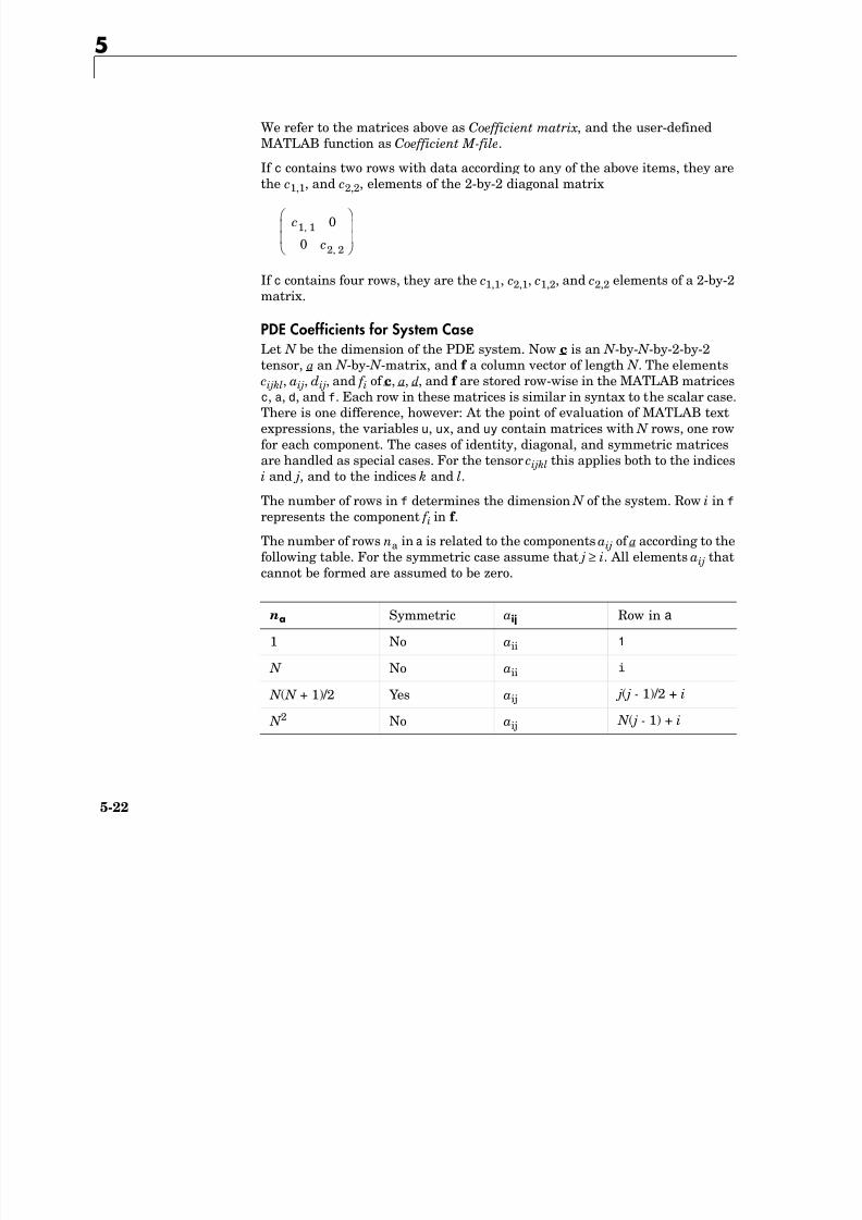
8/21/2019 matlab pde solving.pdf
http://slidepdf.com/reader/full/matlab-pde-solvingpdf 208/290
5-22
If c contains four rows, they are the c1,1, c2,1, c1,2, and c2,2 elements of a 2-by-2
matrix.
PDE Coefficients for System CaseLet N be the dimension of the PDE system. Now c is an N -by- N -by-2-by-2tensor, a an N -by- N -matrix, and f a column vector of length N . The elementscijkl, aij, dij, and f i of c, a, d , and f are stored row-wise in the MATLAB matricesc, a, d, and f. Each row in these matrices is similar in syntax to the scalar case.There is one difference, however: At the point of evaluation of MATLAB textexpressions, the variables u, ux, and uy contain matrices with N rows, one rowfor each component. The cases of identity, diagonal, and symmetric matricesare handled as special cases. For the tensor cijkl this applies both to the indicesi and j, and to the indices k and l.
The number of rows in f determines the dimension N of the system. Row i in f represents the component f i in f .
The number of rows n
a
ina is related to the components aij of a according to thefollowing table. For the symmetric case assume that j ≥ i. All elements aij thatcannot be formed are assumed to be zero.
na Symmetric aij Row in a
1 No aii 1
N No aii i
N ( N + 1)/2 Yes aij j( j - 1)/2 + i
N 2 No aij N ( j - 1) + i
c1 1, 0
0 c2 2,# $% &% &
An example of how a is stored in a can be found below.
The coding of c in c is determined by the dimension N and the number of rows
nc in c. The number of rows nc in c is matched to the function of N in the firstcolumn in the table below — sequentially from the first line to the last line.The first match determines the type of coding of c. This actually means that forsome small values, 2 ≤ N ≤ 4, the coding is only determined by the order in
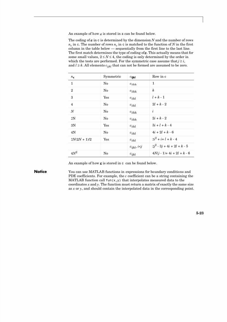
8/21/2019 matlab pde solving.pdf
http://slidepdf.com/reader/full/matlab-pde-solvingpdf 209/290
5-23
which the tests are performed. For the symmetric case assume that j ≥ i,and l ≥ k. All elements cijkl that can not be formed are assumed to be zero.
An example of how c is stored in c can be found below.
Notice You can use MATLAB functions in expressions for boundary conditions andPDE coefficients. For example, the c coefficient can be a string containing the
MATLAB function call fun(x,y) that interpolates measured data to thecoordinates x and y. The function must return a matrix of exactly the same sizeas x or y, and should contain the interpolated data in the corresponding point.
nc Symmetric cijkl Row in c1 No ciikk 1
2 No ciikk k
3 Yes ciikl l + k - 1
4 No ciikl 2l + k - 2
N No ciikk i
2N No ciikk 2i + k - 2
3N Yes ciikl 3i + l + k - 4
4N No ciikl 4i + 2l + k - 6
2 N (2 N + 1)/2 Yes ciikl 2i2 + i+ l + k - 4
cijkl, i< j 2 j2 - 3 j + 4i + 2l + k - 5
4 N 2 No cijkl 4 N ( j - 1)+ 4i + 2l + k - 6
5
Examples Example 1Solve the equation on the geometry defined by the L-shaped
membrane. Use Dirichlet boundary conditions u = 0 on . Finally plot thesolution.
[p,e,t]=initmesh('lshapeg','Hmax',0.2);
[p,e,t]=refinemesh('lshapeg',p,e,t);
u∆ – 1=
Ω∂

8/21/2019 matlab pde solving.pdf
http://slidepdf.com/reader/full/matlab-pde-solvingpdf 210/290
5-24
[p, , ] ( p g ,p, , );
u=assempde('lshapeb',p,e,t,1,0,1);
pdesurf(p,t,u)
Example 2Consider Poisson’s equation on the unit circle with unit point source at theorigin. The exact solution
is known for this problem. We define the function f=circlef(p,t,u,time) forcomputing the right-hand side. circlef returns zero for all triangles except for
the one located at the origin; for that triangle it returns 1/ a, where a is thetriangle area. pdedemo7 performs a full demonstration of the problem withadaptive solution.
u1
2π------ – r( )log=
−1
−0.5
0
0.5
1
−1
−0.5
0
0.5
1
0
0.2
0.4
0.6
0.8
1
Example 3We study how the matrices a (and also d ) are stored in the MATLAB matrix a
for system case N = 3.
na = 1: a(1) 0 0 na = 3: a(1) 0 0
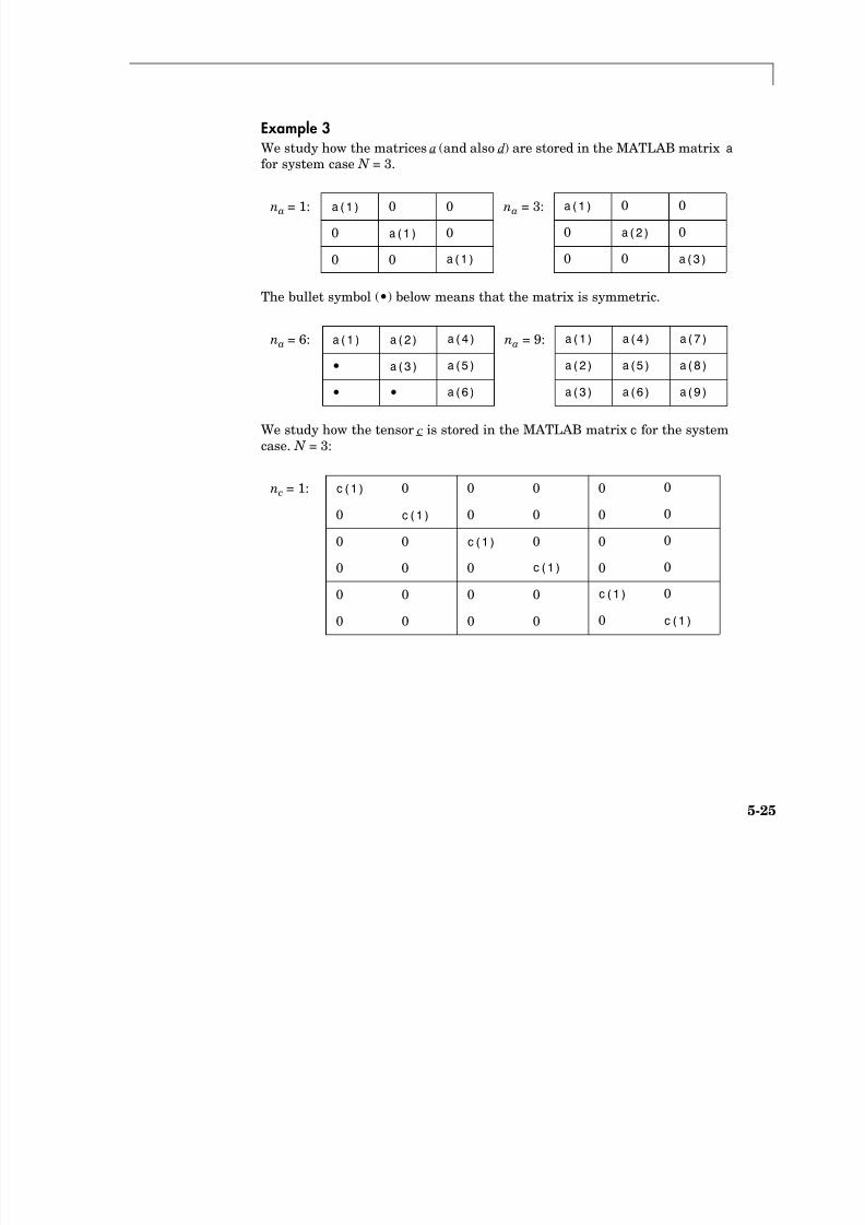
8/21/2019 matlab pde solving.pdf
http://slidepdf.com/reader/full/matlab-pde-solvingpdf 211/290
5-25
The bullet symbol (•) below means that the matrix is symmetric.
We study how the tensor c is stored in the MATLAB matrix c for the systemcase. N = 3:
0 a(1) 0 0 a(2) 0
0 0 a(1) 0 0 a(3)
na = 6: a(1) a(2) a(4) na = 9: a(1) a(4) a(7)
• a(3) a(5) a(2) a(5) a(8)
• • a(6) a(3) a(6) a(9)
nc = 1: c(1) 0 0 0 0 0
0 c(1) 0 0 0 0
0 0 c(1) 0 0 0
0 0 0 c(1) 0 0
0 0 0 0 c(1) 0
0 0 0 0 0 c(1)
5
nc = 2: c(1) 0 0 0 0 0
0 c(2) 0 0 0 00 0 c(1) 0 0 0
0 0 0 c(2) 0 0
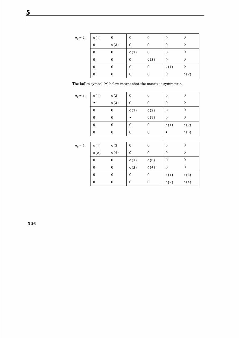
8/21/2019 matlab pde solving.pdf
http://slidepdf.com/reader/full/matlab-pde-solvingpdf 212/290
5-26
The bullet symbol (•) below means that the matrix is symmetric.
0 0 0 0 c(1) 0
0 0 0 0 0 c(2)
nc = 3: c(1) c(2) 0 0 0 0
• c(3) 0 0 0 0
0 0 c(1) c(2) 0 0
0 0 • c(3) 0 00 0 0 0 c(1) c(2)
0 0 0 0 • c(3)
nc = 4: c(1) c(3) 0 0 0 0
c(2) c(4) 0 0 0 00 0 c(1) c(3) 0 0
0 0 c(2) c(4) 0 0
0 0 0 0 c(1) c(3)
0 0 0 0 c(2) c(4)
The case nc = 3 takes precedence over the case nc = N , and the form nc = N thuscannot be used.
nc = 6: c(1) 0 0 0 0 0
0 c(2) 0 0 0 0
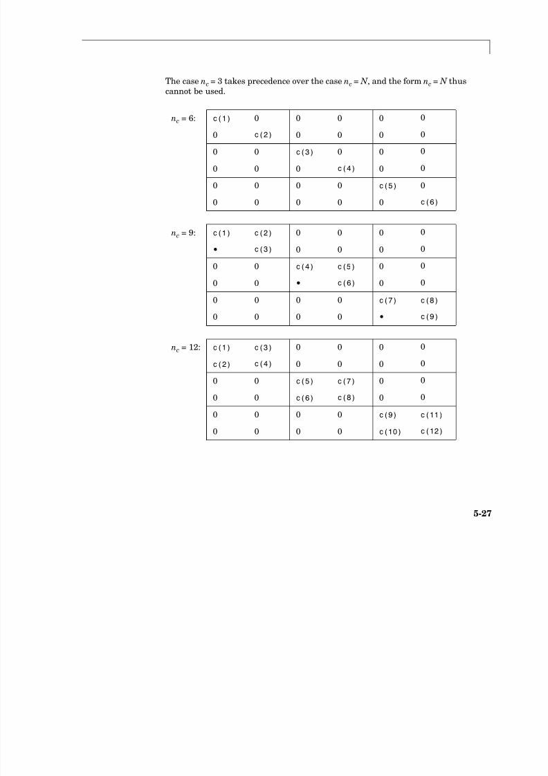
8/21/2019 matlab pde solving.pdf
http://slidepdf.com/reader/full/matlab-pde-solvingpdf 213/290
5-27
0 0 c(3) 0 0 0
0 0 0 c(4) 0 0
0 0 0 0 c(5) 00 0 0 0 0 c(6)
nc = 9: c(1) c(2) 0 0 0 0
• c(3) 0 0 0 0
0 0 c(4) c(5) 0 00 0 • c(6) 0 0
0 0 0 0 c(7) c(8)
0 0 0 0 • c(9)
nc = 12: c(1) c(3) 0 0 0 0c(2) c(4) 0 0 0 0
0 0 c(5) c(7) 0 0
0 0 c(6) c(8) 0 0
0 0 0 0 c(9) c(11)
0 0 0 0 c(10) c(12)
5
nc = 21: c(1) c(2) c(4) c(6) c(11) c(13)
• c(3) c(5) c(7) c(12) c(14)
• • c(8) c(9) c(15) c(17)
• • • c(10) c(16) c(18)

8/21/2019 matlab pde solving.pdf
http://slidepdf.com/reader/full/matlab-pde-solvingpdf 214/290
5-28
See Also initmesh, refinemesh, pdebound, assema, assemb
• • • • c(19) c(20)
• • • • • c(21)
nc = 36: c(1) c(3) c(13) c(15) c(25) c(27)
c(2) c(4) c(14) c(16) c(26) c(28)
c(5) c(7) c(17) c(19) c(29) c(31)
c(6) c(8) c(18) c(20) c(30) c(32)
c(9) c(11) c(21) c(23) c(33) c(35)
c(10) c(12) c(22) c(24) c(34) c(36)
5csgchkPurpose Check validity of Geometry Description matrix
Syntax gstat=csgchk(gd,xlim,ylim)gstat=csgchk(gd)
Description gstat=csgchk(gd,xlim,ylim) checks if the solid objects in the GeometryDescription matrix gd are valid given optional real numbers xlim and ylim as
8/21/2019 matlab pde solving.pdf
http://slidepdf.com/reader/full/matlab-pde-solvingpdf 215/290
5-29
Description matrix gd are valid, given optional real numbers xlim and ylim ascurrent length of the x- and y-axis, and using a special format for polygons. Fora polygon, the last vertex coordinate can be equal to the first one, to indicate aclosed polygon. If xlim and ylim are specified and if the first and the last
vertices are not equal, the polygon is considered as closed if these vertices arewithin a certain “closing distance.” These optional input arguments are meantto be used only when calling csgchk from pdetool.
gstat=csgchk(gd) is identical to the above call, except for using the sameformat of gd that is used by decsg. This call is recommended when usingcsgchk as a command-line function.
gstat is a row vector of integers that indicates the validity status of the
corresponding solid objects, i.e., columns, in gd.For a circle solid, gstat=0 indicates that the circle has a positive radius, 1 indicates a nonpositive radius, and 2 indicates that the circle is not unique.
For a polygon, gstat=0 indicates that the polygon is closed and does notintersect itself, i.e., it has a well-defined, unique interior region. 1 indicates anopen and non-self-intersecting polygon, 2 indicates a closed andself-intersecting polygon, and 3 indicates an open and self-intersecting
polygon.For a rectangle solid, gstat is identical to that of a polygon. This is so becausea rectangle is considered as a polygon by csgchk.
For an ellipse solid, gstat=0 indicates that the ellipse has positive semiaxes, 1 indicates that at least one of the semiaxes is nonpositive, and 2 indicates thatthe ellipse is not unique.
Ifgstat
consists of zero entries only, thengd
is valid and can be used as inputargument by decsg.
See Also decsg
5
5csgdelPurpose Delete borders between minimal regions
Syntax [dl1,bt1]=csgdel(dl,bt,bl)[dl1,bt1]=csgdel(dl,bt)
Description [dl1,bt1]=csgdel(dl,bt,bl) deletes the border segments in the list bl. If theconsistency of the Decomposed Geometry matrix is not preserved by deleting
8/21/2019 matlab pde solving.pdf
http://slidepdf.com/reader/full/matlab-pde-solvingpdf 216/290
5-30
consistency of the Decomposed Geometry matrix is not preserved by deletingthe elements in the list bl, additional border segments are deleted. Boundarysegments cannot be deleted.
For an explanation of the concepts or border segments, boundary segments,and minimal regions, see decsg on page 5-31.
dl and dl1 are Decomposed Geometry matrices. For a description of theDecomposed Geometry matrix, see decsg . The format of the Boolean tables bt and bt1 is also described in the entry on decsg.
[dl1,bt1]=csgdel(dl,bt) deletes all border segments.
See Also decsg, csgchk
5decsgPurpose Decompose Constructive Solid Geometry into minimal regions
Syntax dl=decsg(gd)dl=decsg(gd,sf,ns)
[dl,bt]=decsg(gd)
[dl,bt]=decsg(gd,sf,ns)
[dl bt dl1 bt1 msb]=decsg(gd)
8/21/2019 matlab pde solving.pdf
http://slidepdf.com/reader/full/matlab-pde-solvingpdf 217/290
5-31
[dl,bt,dl1,bt1,msb] decsg(gd)
[dl,bt,dl1,bt1,msb]=decsg(gd,sf,ns)
Description This function analyzes the Constructive Solid Geometry model (CSG model)
that you draw. It analyzes the CSG model, constructs a set of disjoint minimalregions, bounded by boundary segments and border segments, and optionallyevaluates a set formula in terms of the objects in the CSG model. We often referto the set of minimal regions as the decomposed geometry. The decomposedgeometry makes it possible for other toolbox functions to “understand” thegeometry you specify. For plotting purposes a second set of minimal regionswith a connected boundary is constructed.
The graphical user interface pdetool uses decsg for many purposes. Each timea new solid object is drawn or changed, pdetool calls decsg in order to be ableto draw the solid objects and minimal regions correctly. The Delaunaytriangulation algorithm, initmesh, also uses the output of decsg to generate aninitial mesh.
dl=decsg(gd,sf,ns) decomposes the CSG model gd into the decomposedgeometry dl. The CSG model is represented by the Geometry Descriptionmatrix, and the decomposed geometry is represented by the DecomposedGeometry matrix. decsg returns the minimal regions that evaluate to true forthe set formula sf. The Name Space matrix ns is a text matrix that relates thecolumns in gd to variable names in sf.
dl=decsg(gd) returns all minimal regions. (The same as letting sf correspondto the union of all objects in gd.)
[dl,bt]=decsg(gd) and [dl,bt]=decsg(gd,sf,ns) additionally return a
Boolean table that relates the original solid objects to the minimal regions. Acolumn in bt corresponds to the column with the same index in gd. A row in bt corresponds to a minimal region index.
5
[dl,bt,dl1,bt1,msb]=decsg(gd) and[dl,bt,dl1,bt1,msb]=decsg(gd,sf,ns) return a second set of minimal
regionsdl1
with a corresponding Boolean tablebt1
. This second set of minimalregions all have a connected boundary. These minimal regions can be plottedby using MATLAB patch objects. The second set of minimal regions haveborders that may not have been induced by the original solid objects. Thisoccurs when two or more groups of solid objects have nonintersectingb d i
8/21/2019 matlab pde solving.pdf
http://slidepdf.com/reader/full/matlab-pde-solvingpdf 218/290
5-32
boundaries.
The calling sequences additionally return a sequence msb of drawingcommands for each second minimal region. The first row contains the number
of edge segment that bounds the minimal region. The additional rows containthe sequence of edge segments from the Decomposed Geometry matrix thatconstitutes the bound. If the index edge segment label is greater than the totalnumber of edge segments, it indicates that the total number of edge segmentsshould be subtracted from the contents to get the edge segment label numberand the drawing direction is opposite to the one given by the DecomposedGeometry matrix.
Geometry Description Matrix The Geometry Description matrix gd describes the CSG model that you drawusing pdetool. The current Geometry Description matrix can be madeavailable to the MATLAB main workspace by selecting the Export Geometry
Description, Set Formula, Labels . . . option from the Draw menu in pdetool.
Each column in the Geometry Description matrix corresponds to an object inthe CSG model. Four types of solid objects are supported. The object type isspecified in row 1:
•For the circle solid, row one contains 1, and the second and third row containthe center x- and y-coordinates, respectively. Row four contains the radius ofthe circle.
•For a polygon solid, row one contains 2, and the second row contains thenumber, n, of line segments in the boundary of the polygon. The following n rows contain the x-coordinates of the starting points of the edges, and thefollowing n rows contain the y-coordinates of the starting points of the edges.
•For a rectangle solid, row one contains 3. The format is otherwise identicalto the polygon format.
•For an ellipse solid, row one contains 4, the second and third row containsthe center x- and y-coordinates, respectively. Rows four and five contain the
semiaxes of the ellipse. The rotational angle of the ellipse is stored in row six.
Set Formulasf contains a set formula expressed with the set of variables listed in ns. Theoperators ‘+’, ‘*’, and ‘–’ correspond to the set operations union, intersection,
8/21/2019 matlab pde solving.pdf
http://slidepdf.com/reader/full/matlab-pde-solvingpdf 219/290
5-33
operators + , , and correspond to the set operations union, intersection,and set difference, respectively. The precedence of the operators ‘+’ and ‘*’ is thesame. ‘–’ has higher precedence. The precedence can be controlled withparentheses.
Name Space Matrix The Name Space matrix ns relates the columns in gd to variable names in sf.Each column in ns contains a sequence of characters, padded with spaces. Eachsuch character column assigns a name to the corresponding geometric object ingd. This way we can refer to a specific object in gd in the set formula sf.
Decomposed Geometry Matrix The Decomposed Geometry matrix dl contains a representation of thedecomposed geometry in terms of disjointed minimal regions that have beenconstructed by the decsg algorithm. Each edge segment of the minimal regionscorresponds to a column in dl. We refer to edge segments between minimalregions as border segments and outer boundaries as boundary segments. Ineach such column rows two and three contain the starting and ending x-coordinate, and rows four and five the corresponding y-coordinate. Rows sixand seven contain left and right minimal region labels with respect to thedirection induced by the start and end points (counter clockwise direction oncircle and ellipse segments). There are three types of possible edge segments ina minimal region:
•For circle edge segments row one is 1. Rows eight and nine contain thecoordinates of the center of the circle. Row 10 contains the radius.
•For line edge segments row one is 2.
•For ellipse edge segments row one is 4. Rows eight and nine contain thecoordinates of the center of the ellipse. Rows 10 and 11 contain the semiaxesof the ellipse, respectively. The rotational angle of the ellipse is stored inrow 12.
5
Examples The command sequence below starts pdetool and draws a unit circle and a unitsquare.
pdecirc(0,0,1)pderect([0 1 0 1])
Insert the set formula C1 SQ1. Export the Geometry Description matrix, setformula, and Name Space matrix to the MATLAB main workspace by selecting
8/21/2019 matlab pde solving.pdf
http://slidepdf.com/reader/full/matlab-pde-solvingpdf 220/290
5-34
the Export Geometry Description . . . option from the Draw menu. Then type
[dl,bt]=decsg(gd,sf,ns);
dl =
2.0000 2.0000 1.0000 1.0000 1.0000
0 0 1.0000 0.0000 0.0000
1.0000 0 0.0000 1.0000 1.0000
0 1.0000 0.0000 1.0000 1.0000
0 0 1.0000 0 0.0000
0 0 1.0000 1.0000 1.0000
1.0000 1.0000 0 0 0
0 0 0 0 0
0 0 0 0 00 0 1.0000 1.0000 1.0000
bt =
1 0
Note that there is one minimal region, with five edge segments, three circleedge segments, and two line edge segments.
Algorithm The algorithm consists of the following steps:
1 Determine the intersection points between the borders of the model objects.
2 For each intersection point, sort the incoming edge segments on angle andcurvature.
3 Determine if the induced graph is connected. If not, add some appropriate
edges, and redo algorithm from step 1.
4 Cycle through edge segments of minimal regions.
5 For each original region, determine minimal regions inside it.
6 Organize output and remove the additional edges.
Note The input CSG model is not checked for correctness. It is assumed thatno circles or ellipses are identical or degenerated and that no lines have zerolength. Polygons must not be selfintersecting. Use the function csgchk tocheck the CSG model.
8/21/2019 matlab pde solving.pdf
http://slidepdf.com/reader/full/matlab-pde-solvingpdf 221/290
5-35
check the CSG model.
Diagnostics NaN is returned if the set formula sf cannot be evaluated.See Also pdetool, pdegeom, pdebound, wgeom, wbound, pdecirc, pderect, pdepoly,
pdeellip, csgchk, csgdel
5
5dst, idstPurpose Discrete sine transform
Syntax y=dst(x)x=idst(y)
Description y=dst(x) computes the discrete sine transform of the columns of x. For bestperformance speed, the number of rows in x should be 2m - 1, for some integer
8/21/2019 matlab pde solving.pdf
http://slidepdf.com/reader/full/matlab-pde-solvingpdf 222/290
5-36
m.
y=dst(x,n) pads or truncates the vector x to length n before transforming.
If x is a matrix, the dst operation is applied to each column.
x=idst(y) calculates the inverse discrete sine transform of the columns of y.For best performance speed, the number of rows in y should be 2m - 1, for someinteger m.
x=idst(y,n) pads or truncates the vector y to length n before transforming.
If y is a matrix, the idst operation is applied to each column.
See Also poisolv, poiasma, poiindex
5hyperbolicPurpose Solve hyperbolic PDE problem
Syntax u1=hyperbolic(u0,ut0,tlist,b,p,e,t,c,a,f,d)u1=hyperbolic(u0,ut0,tlist,b,p,e,t,c,a,f,d,rtol)
u1=hyperbolic(u0,ut0,tlist,b,p,e,t,c,a,f,d,rtol,atol)
u1=hyperbolic(u0,ut0,tlist,K,F,B,ud,M)
u1=hyperbolic(u0,ut0,tlist,K,F,B,ud,M,rtol)
8/21/2019 matlab pde solving.pdf
http://slidepdf.com/reader/full/matlab-pde-solvingpdf 223/290
5-37
u1=hyperbolic(u0,ut0,tlist,K,F,B,ud,M,rtol,atol)
Description u1=hyperbolic(u0,ut0,tlist,b,p,e,t,c,a,f,d) produces the solution to
the FEM formulation of the scalar PDE problem
or the system PDE problem
on a mesh described by p, e, and t, with boundary conditions given by b, andwith initial value u0 and initial derivative ut0.
In the scalar case, each row in the solution matrix u1 is the solution at thecoordinates given by the corresponding column in p. Each column in u1 is thesolution at the time given by the corresponding item in tlist. For a system ofdimension N with n
p node points, the first n
p rows of u1 describe the first
component of u, the following n p rows of u1 describe the second component ofu, and so on. Thus, the components of u are placed in blocks u as N blocks ofnode point rows.
b describes the boundary conditions of the PDE problem. b can be either aBoundary Condition matrix or the name of a Boundary M-file. The boundaryconditions can depend on t, the time. The formats of the Boundary Conditionmatrix and Boundary M-file are described in the entries on assemb andpdebound, respectively.The geometry of the PDE problem is given by the mesh data p, e, and t. Fordetails on the mesh data representation, see initmesh on page 5-40.
d∂
2u
∂t2
--------- ∇ c∇u( ) au+⋅ – f on Ω=
d
∂2u
∂t2---------
∇ c ∇u⊗( ) au+⋅ – f on Ω=
5
The coefficients c, a, d, and f of the PDE problem can be given in a variety ofways. The coefficients can depend on t, the time. For a complete listing of all
options, see assempde on page 5-19.atol and rtol are absolute and relative tolerances that are passed to the ODEsolver.
u1=hyperbolic(u0,ut0,tlist,K,F,B,ud,M) produces the solution to the ODE
8/21/2019 matlab pde solving.pdf
http://slidepdf.com/reader/full/matlab-pde-solvingpdf 224/290
5-38
problem
with initial values for u being u0 and ut0.
Examples Solve the wave equation
on a square geometry -1 ≤ x,y ≤ 1 (squareg), with Dirichlet boundary conditionsu = 0 for x = ±1, and Neumann boundary conditions
for y = ±1 (squareb3). Choose
and
Compute the solution at times 0, 1/6, 1/3, ... , 29/6, 5.
[p,e,t]=initmesh('squareg');
x=p(1,:)';
y=p(2,:)';
u0=atan(cos(pi/2*x));
ut0=3*sin(pi*x).*exp(cos(pi*y));
B′ MB
d2ui
dt2------------ K + ui⋅ F ,= u Bui ud+=
∂2u
∂t2
--------- u∆=
∂u
∂n------ 0=
u 0( ) Π x( )cos( )atan=
du 0( )
dt---------------- 3 Π x( ) Π y( )cos( )expsin=
tlist=linspace(0,5,31);
uu=hyperbolic(u0,ut0,tlist,'squareb3',p,e,t,1,0,0,1);
The file pdedemo6 contains a complete example with animation.
Note In expressions for boundary conditions and PDE coefficients, thesymbol t is used to denote time. The variable t is often used to store the

8/21/2019 matlab pde solving.pdf
http://slidepdf.com/reader/full/matlab-pde-solvingpdf 225/290
5-39
triangle matrix of the mesh. You can use any variable to store the trianglematrix, but in PDE toolbox expressions, t always denotes time.
See Also assempde, parabolic
5
5initmeshPurpose Create initial triangular mesh
Syntax [p,e,t]=initmesh(g)[p,e,t]=initmesh(g,'PropertyName',PropertyValue,...)
Description [p,e,t]=initmesh(g) returns a triangular mesh using the geometryspecification function g. It uses a Delaunay triangulation algorithm. The meshi i d t i d f th h f th g t
8/21/2019 matlab pde solving.pdf
http://slidepdf.com/reader/full/matlab-pde-solvingpdf 226/290
5-40
size is determined from the shape of the geometry.
g describes the geometry of the PDE problem. g can either be a Decomposed
Geometry matrix or the name of a Geometry M-file. The formats of theDecomposed Geometry matrix and Geometry M-file are described in the entrieson decsg and pdegeom, respectively.
The outputs p, e, and t are the mesh data.
In the Point matrix p, the first and second rows contain x- and y-coordinates ofthe points in the mesh.
In the Edge matrix e, the first and second rows contain indices of the starting
and ending point, the third and fourth rows contain the starting and endingparameter values, the fifth row contains the edge segment number, and thesixth and seventh row contain the left- and right-hand side subdomainnumbers.
In the Triangle matrix t, the first three rows contain indices to the cornerpoints, given in counter clockwise order, and the fourth row contains thesubdomain number.
The following property name/property value pairs are allowed.
Property Value Default Description
Hmax numeric estimate Maximum edge size
Hgrad numeric 1.3 Mesh growth rate
Box on|off off Preserve bounding box
Init on|off off Edge triangulation
The Hmax property controls the size of the triangles on the mesh. initmesh creates a mesh where no triangle side exceeds Hmax.
Jiggle off|mean|min mean Call jigglemeshJiggleIter numeric 10 Maximum iterations
Property Value Default Description
8/21/2019 matlab pde solving.pdf
http://slidepdf.com/reader/full/matlab-pde-solvingpdf 227/290
5-41
g
The Hgrad property determines the mesh growth rate away from a small partof the geometry. The default value is 1.3, i.e., a growth rate of 30%. Hgrad must
be between 1 and 2.Both the Box and Init property are related to the way the mesh algorithmworks. By turning on Box you can get a good idea of how the mesh generationalgorithm works within the bounding box. By turning on Init you can see theinitial triangulation of the boundaries. By using the command sequence
[p,e,t]=initmesh(dl,'hmax',inf,'init','on');
[uxy,tn,a2,a3]=tri2grid(p,t,zeros(size(p,2)),x,y);
n=t(4,tn);
you can determine the subdomain number n of the point xy. If the point isoutside the geometry, tn is NaN and the command n=t(4,tn) results in afailure.
The Jiggle property is used to control whether jiggling of the mesh should beattempted (see jigglemesh on page 5-44 for details). Jiggling can be done untilthe minimum or the mean of the quality of the triangles decreases. JiggleIter
can be used to set an upper limit on the number of iterations.
Algorithm initmesh implements a Delaunay triangulation algorithm:
1 Place node points on the edges.
2 Enclose geometry in bounding box.
3 Triangulate edges.
4 Check that the triangulation respects boundaries.
5 Insert node points into centers of circumscribed circles of large triangles.
5
6 Repeat from step 4 if Hmax not yet achieved.
7 Remove bounding box.
Examples Make a simple triangular mesh of the L-shaped membrane in pdetool.Before you do anything in pdetool, set the Maximum edge size to inf in theMesh Parameters dialog box. You open the dialog box by selecting theParameters . . . option from the Mesh menu. Also select the items Show Node
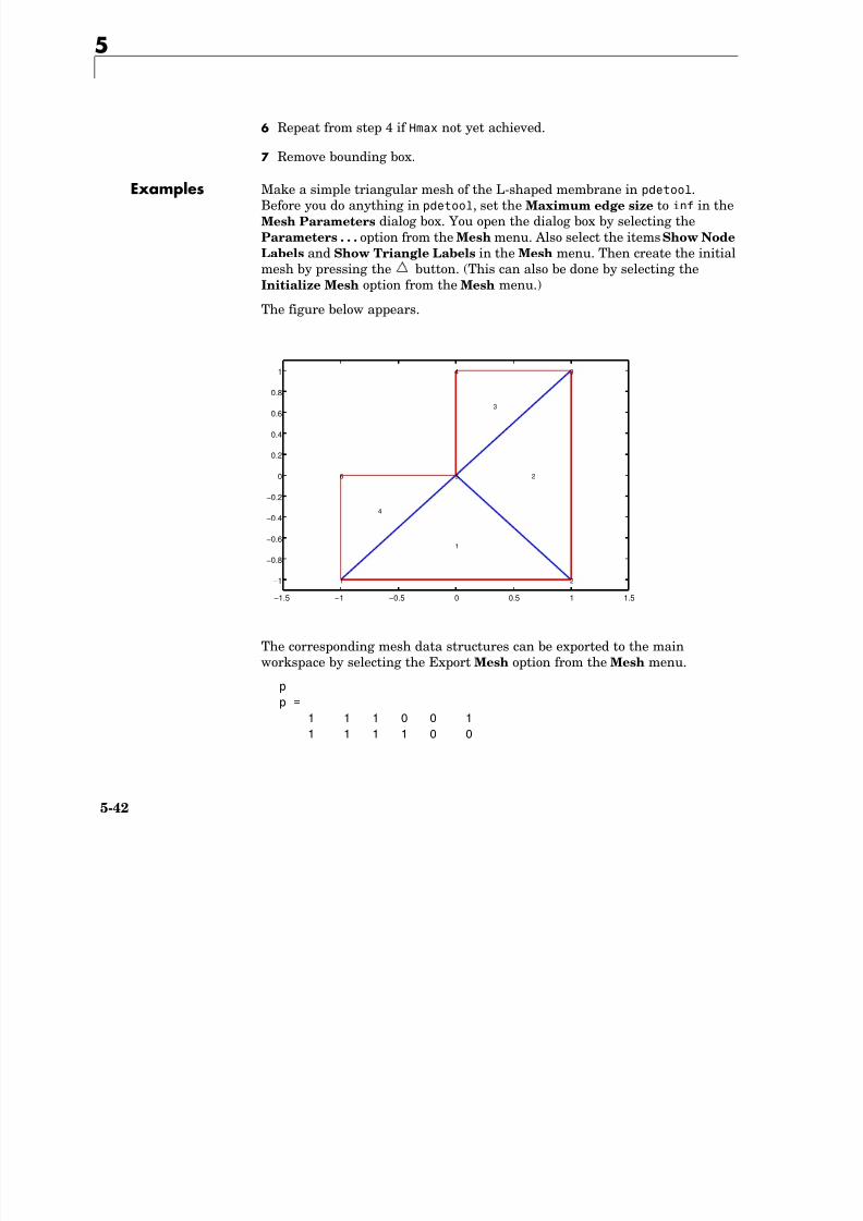
8/21/2019 matlab pde solving.pdf
http://slidepdf.com/reader/full/matlab-pde-solvingpdf 228/290
5-42
pLabels and Show Triangle Labels in the Mesh menu. Then create the initialmesh by pressing the button. (This can also be done by selecting theInitialize Mesh option from the Mesh menu.)
The figure below appears.
The corresponding mesh data structures can be exported to the mainworkspace by selecting the Export Mesh option from the Mesh menu.
pp =
1 1 1 0 0 1
1 1 1 1 0 0
−1.5 −1 −0.5 0 0.5 1 1.5
−1
−0.8
−0.6
−0.4
−0.2
0
0.2
0.4
0.6
0.8
1
1 2
34
56
1
2
3
4
e
e =
1 2 3 4 5 6
2 3 4 5 6 1
0 0 0 0 0 0
1 1 1 1 1 1
1 2 3 4 5 6
1 1 1 1 1 1
8/21/2019 matlab pde solving.pdf
http://slidepdf.com/reader/full/matlab-pde-solvingpdf 229/290
5-43
0 0 0 0 0 0
t
t =
1 2 3 1
2 3 4 5
5 5 5 6
1 1 1 1
See Also decsg, pdegeom, jigglemesh, refinemesh
Reference George, P. L., Automatic Mesh Generation — Application to Finite Element
Methods, Wiley, 1991.
5
5jigglemeshPurpose Jiggle internal points of a triangular mesh
Syntax p1=jigglemesh(p,e,t)p1=jigglemesh(p,e,t,'PropertyName',PropertyValue,...)
Description p1=jigglemesh(p,e,t) jiggles the triangular mesh by adjusting the node pointpositions. The quality of the mesh normally increases.
8/21/2019 matlab pde solving.pdf
http://slidepdf.com/reader/full/matlab-pde-solvingpdf 230/290
5-44
The following property name/property value pairs are allowed.
Each mesh point that is not located on an edge segment is moved toward thecenter of mass of the polygon formed by the adjacent triangles. This process isrepeated according to the settings of the Opt and Iter variables:
•When Opt is set to off this process is repeated Iter times (default: 1).
•When Opt is set to mean the process is repeated until the mean trianglequality does not significantly increase, or until the bound Iter is reached(default: 20).
•When Opt is set to min the process is repeated until the minimum trianglequality does not significantly increase, or until the bound Iter is reached
(default: 20).Examples Create a triangular mesh of the L-shaped membrane, first without jiggling,
and then jiggle the mesh.
[p,e,t]=initmesh('lshapeg','jiggle','off');
q=pdetriq(p,t);
pdeplot(p,e,t,'xydata',q,'colorbar','on','xystyle','flat')
p1=jigglemesh(p,e,t,'opt','mean','iter',inf);
q=pdetriq(p1,t);pdeplot(p1,e,t,'xydata',q,'colorbar','on','xystyle','flat')
See Also initmesh, pdetriq
Property Value Default Description
Opt off|mean|min mean Optimization method
Iter numeric 1 or 20 (see below) Maximum iterations
5parabolicPurpose Solve parabolic PDE problem
Syntax u1=parabolic(u0,tlist,b,p,e,t,c,a,f,d)u1=parabolic(u0,tlist,b,p,e,t,c,a,f,d,rtol)
u1=parabolic(u0,tlist,b,p,e,t,c,a,f,d,rtol,atol)
u1=parabolic(u0,tlist,K,F,B,ud,M)
u1=parabolic(u0,tlist,K,F,B,ud,M,rtol)
u1=parabolic(u0 tlist K F B ud M rtol atol)
8/21/2019 matlab pde solving.pdf
http://slidepdf.com/reader/full/matlab-pde-solvingpdf 231/290
5-45
u1=parabolic(u0,tlist,K,F,B,ud,M,rtol,atol)
Description u1=parabolic(u0,tlist,g,b,p,e,t,c,a,f,d) produces the solution to the
FEM formulation of the scalar PDE problem
or the system PDE problem
on a mesh described by p, e, and t, with boundary conditions given by b, andwith initial value u0.
For the scalar case, each row in the solution matrix u1 is the solution at thecoordinates given by the corresponding column in p. Each column in u1 is thesolution at the time given by the corresponding item in tlist. For a system ofdimension N with n p node points, the first n p rows of u1 describe the firstcomponent of u, the following n p rows of u1 describe the second component of
u, and so on. Thus, the components of u are placed in the vector u as N blocksof node point rows.
b describes the boundary conditions of the PDE problem. b can be either aBoundary Condition matrix or the name of a Boundary M-file. The boundaryconditions can depend on t, the time. The formats of the Boundary Conditionmatrix and Boundary M-file are described in the entries on assemb andpdebound, respectively.
The geometry of the PDE problem is given by the mesh data p, e, and t. Fordetails on the mesh data representation, see initmesh on page 5-40.
d∂u
∂t------ ∇ c∇u( ) au+⋅ – f on Ω=
d∂u
∂t------ ∇ c ∇u⊗( ) au+⋅ – f on Ω=
5
The coefficients c, a, d, and f of the PDE problem can be given in a variety ofways. The coefficients can depend on t, the time. For a complete listing of all
options, seeassempde
on page 5-19.atol and rtol are absolute and relative tolerances that are passed to the ODEsolver.
u1=parabolic(u0,tlist,K,F,B,ud,M) produces the solution to the ODEproblem
8/21/2019 matlab pde solving.pdf
http://slidepdf.com/reader/full/matlab-pde-solvingpdf 232/290
5-46
problem
with initial value for u being u0.
Examples Solve the heat equation
on a square geometry -1 ≤ x,y ≤ 1 (squareg). Choose u(0) = 1 on the disk x
2
+ y2
< 0.42, and u(0) = 0 otherwise. Use Dirichlet boundary conditions u = 0(squareb1). Compute the solution at times linspace(0,0.1,20).
[p,e,t]=initmesh('squareg');
[p,e,t]=refinemesh('squareg',p,e,t);
u0=zeros(size(p,2),1);
ix=find(sqrt(p(1,:).^2+p(2,:).^2)<0.4);
u0(ix)=ones(size(ix));
tlist=linspace(0,0.1,20);u1=parabolic(u0,tlist,'squareb1',p,e,t,1,0,1,1);
Note In expressions for boundary conditions and PDE coefficients, thesymbol t is used to denote time. The variable t is often used to store thetriangle matrix of the mesh. You can use any variable to store the trianglematrix, but in PDE Toolbox expressions, t always denotes time.
See Also assempde, hyperbolic
B′ MBdu i
dt
--------- K + ui⋅ F ,= u Bui ud+=
∂u
∂t------ u∆=
5pdeadgscPurpose Select triangles using a relative tolerance criterion
Syntax bt=pdeadgsc(p,t,c,a,f,u,errf,tol)
Description bt=pdeadgsc(p,t,c,a,f,u,errf,tol) returns indices of triangles to berefined in bt. Used from adaptmesh to select the triangles to be further refined.The geometry of the PDE problem is given by the mesh data p and t. For moredetails, see the entry on initmesh on page 5-40.
8/21/2019 matlab pde solving.pdf
http://slidepdf.com/reader/full/matlab-pde-solvingpdf 233/290
5-47
, y p g
c, a, and f are PDE coefficients. For details, see assempde.
u is the current solution, given as a column vector. For details, see assempde.
errf is the error indicator, as calculated by pdejmps.
tol is a tolerance parameter.
Triangles are selected using the criterion errf>tol*scale, where scale iscalculated as follows:
Let cmax, amax, fmax, and umax be the maximum of c, a, f, and u, respectively.Let l be the side of the smallest axis-aligned square that contains the geometry.
Then scale=max(fmax*l^2,amax*umax*l^2,cmax*umax). The scaling makesthe tol parameter independent of the scaling of the equation and the geometry.
See Also adaptmesh, pdejmps
5
5pdeadworstPurpose Select triangles relative to the worst value
Syntax bt=pdeadworst(p,t,c,a,f,u,errf,wlevel)
Description bt=pdeadworst(p,t,c,a,f,u,errf,wlevel) returns indices of triangles to berefined in bt. Used from adaptmesh to select the triangles to be further refined.
The geometry of the PDE problem is given by the mesh data p and t. Fordetails see initmesh on page 5 40
8/21/2019 matlab pde solving.pdf
http://slidepdf.com/reader/full/matlab-pde-solvingpdf 234/290
5-48
details, see initmesh on page 5-40.
c, a, and f are PDE coefficients. For details, see assempde on page 5-19.
u is the current solution, given as a column vector. For details, see assempde.
errf is the error indicator, as calculated by pdejmps.
wlevel is the error level relative to the worst error. wlevel must be between 0and 1.
Triangles are selected using the criterion errf>wlevel*max(errf).
See Also adaptmesh, pdejmps
5pdearclPurpose Interpolation between parametric representation and arc length
Syntax pp=pdearcl(p,xy,s,s0,s1)
Description pp=pdearcl(p,xy,s,s0,s1) returns parameter values for a parameterizedcurve corresponding to a given set of arc length values.
p is a monotone row vector of parameter values and xy is a matrix with two
8/21/2019 matlab pde solving.pdf
http://slidepdf.com/reader/full/matlab-pde-solvingpdf 235/290
5-49
rows giving the corresponding points on the curve.
The first point of the curve is given the arc length value s0 and the last point
the value s1.On return, pp contains parameter values corresponding to the arc length values specified in s.
The arc length values s, s0, and s1 can be an affine transformation of the arclength.
Examples See the example cardg on the reference page for pdegeom.
See Also pdegeom
5
5pdeboundPurpose Boundary M-file
Syntax [q,g,h,r]=pdebound(p,e,u,time)
Description The Boundary M-file specifies the boundary conditions of a PDE problem.
The most general form of boundary conditions that we can handle is
hu = r
8/21/2019 matlab pde solving.pdf
http://slidepdf.com/reader/full/matlab-pde-solvingpdf 236/290
5-50
⋅ (c ⊗ ∇u) + u = g + h′µ
By the notation ⋅(c ⊗ ∇u) we mean the N -by-1 matrix with (i,1)-component
where the outward normal vector of the boundary . Thereare M Dirichlet conditions and the h-matrix is M -by- N , M ≥ 0. The generalized
Neumann condition contains a source h′µ where the Lagrange multipliers µ iscomputed such that the Dirichlet conditions become satisfied.
The data that you specify is q, g, h, and r.
For M = 0 we say that we have a generalized Neumann boundary condition, for M = N a Dirichlet boundary condition, and for 0 < M < N a mixed boundarycondition.
The Boundary M-file [q,g,h,r]=pdebound(p,e,u,time) computes the valuesof q, g, h, and r, on the a set of edges e.
The matrices p and e are mesh data. e needs only to be a subset of the edgesin the mesh. Details on the mesh data representation can be found in the entryon initmesh.
The input arguments u and time are used for the nonlinear solver and timestepping algorithms, respectively. u and time are empty matrices if the
corresponding parameter is not passed to assemb. If time is NaN and any of thefunction q, g, h, and r depends on time, pdebound must return a matrix ofcorrect size, containing NaNs in all positions, in the corresponding outputargument. It is not possible to explicitly refer to the time derivative of thesolution in the boundary conditions.
n q
n
α( )cos ci j 1 1, , ,∂
∂ x------ α( )cos ci j 1 2, , ,
∂∂ y------ α( )sin ci j 2 1, , ,
∂∂ x------ α( )sin ci j 2 2, , ,
∂∂ y------+ + +# $
' ( u j,
1=
N
"
n α( )cos α( )sin,( )=
The solution u is represented by the solution vector u. Details on therepresentation can be found in the entry on assempde.
q and g must contain the value of q and g on the midpoint of each boundary.Thus we have size(q)=[N^2 ne], where N is the dimension of the system, andne the number of edges in e, and size(g)=[N ne]. For the Dirichlet case, thecorresponding values must be zeros.
h and r must contain the values of h and r at the first point on each edgef ll d b th l t th d i t h dg Th h
8/21/2019 matlab pde solving.pdf
http://slidepdf.com/reader/full/matlab-pde-solvingpdf 237/290
5-51
followed by the value at the second point on each edge. Thus we havesize(h)=[N^2 2*ne], where N is the dimension of the system, and ne thenumber of edges in e, and size(r)=[N 2*ne]. When M < N , h and r must bepadded with N - M rows of zeros.
The elements of the matrices q and h are stored in column-wise ordering in theMATLAB matrices q and h.
Examples For the boundary conditions
the values below should be stored in q, g, h, and r
1
q=[ ... 2 ... ]
2 0
g=[ ... 3 ... ]
4
1 1
h=[ ... 0 ... 0 ... ]
1 1
0 0
r=[ ... 2 ... 2 ... ]
0 0
See Also initmesh, pdegeom, pdesdt, pdeent
1 1 – ( )u 2=
n c u∇⊗( )⋅ 1 22 0# $
% &' (
u+34# $
% &' (
h′µ+=
5
5pdecgradPurpose The flux of a PDE solution
Syntax [cgxu,cgyu]=pdecgrad(p,t,c,u)[cgxu,cgyu]=pdecgrad(p,t,c,u,time)
[cgxu,cgyu]=pdecgrad(p,t,c,u,time,sdl)
Description [cgxu,cgyu]=pdecgrad(p,t,c,u) returns the flux, c ⊗ ∇u, evaluated at thecenter of each triangle.

8/21/2019 matlab pde solving.pdf
http://slidepdf.com/reader/full/matlab-pde-solvingpdf 238/290
5-52
Row i of cgxu contains
Row i of cgyu contains
There is one column for each triangle in t in both cgxu and cgyu.
The geometry of the PDE problem is given by the mesh data p and t. Detailson the mesh data representation can be found in the entry on initmesh.
The coefficient c of the PDE problem can be given in a variety of ways. Acomplete listing of all options can be found in the entry on assempde.
The format for the solution vector u is described in assempde.
The scalar optional argument time is used for parabolic and hyperbolicproblems, if c depends on t, the time.
The optional argument sdl restricts the computation to the subdomains in thelist sdl.
See Also assempde
ci j11∂u j
∂ x--------
j 1=
N
" cij12∂u j
∂ y--------+
ci j21∂u j
∂ x
--------
j 1=
N
"cij22
∂u j
∂ y
--------+
5pdecircPurpose Draw circle
Syntax pdecirc(xc,yc,radius)pdecirc(xc,yc,radius,label)
Description pdecirc(xc,yc,radius) draws a circle with center in (xc,yc) and radiusradius. If the pdetool GUI is not active, it is automatically started, and thecircle is drawn in an empty geometry model.
8/21/2019 matlab pde solving.pdf
http://slidepdf.com/reader/full/matlab-pde-solvingpdf 239/290
5-53
The optional argument label assigns a name to the circle (otherwise a defaultname is chosen).
The state of the Geometry Description matrix inside pdetool is updated toinclude the circle. You can export the Geometry Description matrix frompdetool by using the Export Geometry Description . . . option from the Draw menu. For a details on the format of the Geometry Description matrix, seedecsg on page 5-31.
Examples The command below starts pdetool and draws a unit circle.
pdecirc(0,0,1)
See Also pdeellip, pdepoly, pderect, pdetool
5
5pdecontPurpose Shorthand command for contour plot
Syntax pdecont(p,t,u)pdecont(p,t,u,n)
pdecont(p,t,u,v)
h=pdecont(p,t,u)
h=pdecont(p,t,u,n)
h=pdecont(p,t,u,v)

8/21/2019 matlab pde solving.pdf
http://slidepdf.com/reader/full/matlab-pde-solvingpdf 240/290
5-54
Description pdecont(p,t,u) draws 10 level curves of the PDE node or triangle data u.
h=pdecont(p,t,u) additionally returns handles to the drawn axes objects.If u is a column vector, node data is assumed. If u is a row vector, triangle datais assumed. Triangle data is converted to node data using the functionpdeprtni.
The geometry of the PDE problem is given by the mesh data p and t. For detailson the mesh data representation, see initmesh on page 5-40.
pdecont(p,t,u,n) plots using n levels.pdecont(p,t,u,v) plots using the levels specified by v.
This command is just shorthand for the call
pdeplot(p,[],t,'xydata',u,'xystyle','off','contour','on',...
'levels',n,'colorbar','off');
If you want to have more control over your contour plot, use pdeplot instead ofpdecont.
Examples Plot the contours of the solution to the equation over the geometrydefined by the L-shaped membrane. Use Dirichlet boundary conditions u = 0on .
[p,e,t]=initmesh('lshapeg');
[p,e,t]=refinemesh('lshapeg',p,e,t);
u=assempde('lshapeb',p,e,t,1,0,1);pdecont(p,t,u)
See Also pdeplot, pdemesh, pdesurf
u∆ – 1=
Ω∂
5pdeeigPurpose Solve eigenvalue PDE problem
Syntax [v,l]=pdeeig(b,p,e,t,c,a,d,r)[v,l]=pdeeig(K,B,M,r)
Description [v,l]=pdeeig(b,p,e,t,c,a,d,r) produces the solution to the FEMformulation of the scalar PDE eigenvalue problem
–∆ ⋅ (c∇u) + au = λdu on Ω
8/21/2019 matlab pde solving.pdf
http://slidepdf.com/reader/full/matlab-pde-solvingpdf 241/290
5-55
( )
or the system PDE eigenvalue problem
–∇ ⋅ (c ⊗ ∇u) + au = λdu on Ω
on a geometry described by p, e, and t, and with boundary conditions given byb.
r is a two-element vector, indicating an interval on the real axis. (The left-handside can be Inf.) The algorithm returns all eigenvalues in this interval in l.
v is an eigenvector matrix. For the scalar case each column in v is aneigenvector of solution values at the corresponding node points from p. For asystem of dimension N with n p node points, the first n p rows of v describe thefirst component of v, the following n p rows of v describe the second componentof v, and so on. Thus, the components of v are placed in blocks v as N blocks ofnode point rows.
b describes the boundary conditions of the PDE problem. b can be either aBoundary Condition matrix or the name of a Boundary M-file. The formats of
the Boundary Condition matrix and Boundary M-file are described in theentries on assemb and pdebound, respectively. Note that the eigenvalue PDEproblem is a homogeneous problem, i.e., only boundary conditions where g = 0and r = 0 can be used. The nonhomogeneous part is removed automatically.
The geometry of the PDE problem is given by the mesh data p, e, and t. Fordetails on the mesh data representation, see initmesh on page 5-40.
The coefficients c, a, d of the PDE problem can be given in a wide variety of
ways. In the context of pdeeig the coefficients cannot depend on u nor t, thetime. For a complete listing of all options, see assempde on page 5-19.
[v,l]=pdeeig(K,B,M,r) produces the solution to the generalized sparsematrix eigenvalue problem
5
K ui = λ B′ MBui u = Bui
with Real(λ) in the interval in r.
Examples Compute the eigenvalues less than 100 and corresponding eigenmodes for
–∇u = λu,
on the geometry of the L-shaped membrane. Then display the first andsixteenth eigenmodes.
8/21/2019 matlab pde solving.pdf
http://slidepdf.com/reader/full/matlab-pde-solvingpdf 242/290
5-56
[p,e,t]=initmesh('lshapeg');
[p,e,t]=refinemesh('lshapeg',p,e,t);[p,e,t]=refinemesh('lshapeg',p,e,t);
[v,l]=pdeeig('lshapeb',p,e,t,1,0,1,[ Inf 100]);
l(1) % first eigenvalue
pdesurf(p,t,v(:,1)) % first eigenmode
figure
membrane(1,20,9,9) % the MATLAB function
figure
l(16) % sixteenth eigenvalue
pdesurf(p,t,v(:,16)) % sixteenth eigenmode
Cautionary In the standard case c and d are positive in the entire region. All eigenvaluesare positive, and 0 is a good choice for a lower bound of the interval. The caseswhere either c or d is zero are discussed below.
• If d = 0 in a subregion, the mass matrix M becomes singular. This does notcause any trouble, provided that c > 0 everywhere. The pencil ( K,M ) has a set
of infinite eigenvalues.• If c = 0 in a subregion, the stiffness matrix K becomes singular, and the pencil
( K,M ) has many zero eigenvalues. With an interval containing zero, pdeeig goes on for a very long time to find all the zero eigenvalues. Choose a positivelower bound away from zero but below the smallest nonzero eigenvalue.
• If there is a region where both c = 0 and d = 0, we get a singular pencil. Thewhole eigenvalue problem is undetermined, and any value is equally
plausible as an eigenvalue.Some of the awkward cases are detected by pdeeig. If the shifted matrix issingular, another shift is attempted. If the matrix with the new shift is stillsingular a good guess is that the entire pencil ( K,M ) is singular.
If you try any problem not belonging to the standard case, you must use yourknowledge of the original physical problem to interpret the results from thecomputation.
See Also sptarn
8/21/2019 matlab pde solving.pdf
http://slidepdf.com/reader/full/matlab-pde-solvingpdf 243/290
5-57
5
5pdeellipPurpose Draw ellipse
Syntax pdeellip(xc,yc,a,b,phi)
pdeellip(xc,yc,a,b,phi,label)
Description pdeellip(xc,yc,a,b,phi) draws an ellipse with center in (xc,yc) andsemiaxes a and b. The rotation of the ellipse (in radians) is given by phi. If thepdetool GUI is not active, it is automatically started, and the ellipse is drawnin an empty geometry model
8/21/2019 matlab pde solving.pdf
http://slidepdf.com/reader/full/matlab-pde-solvingpdf 244/290
5-58
in an empty geometry model.
The optional argument label assigns a name to the ellipse (otherwise a default
name is chosen.)The state of the Geometry Description matrix inside pdetool is updated toinclude the ellipse. You can export the Geometry Description matrix frompdetool by selecting the Export Geometry Description . . . option from theDraw menu. For a details on the format of the Geometry Description matrix,see decsg on page 5-31.
Examples The command below starts pdetool and draws an ellipse.pdeellip(0,0,1,0.3,pi/4)
See Also pdecirc, pdepoly, pderect, pdetool
5pdeentPurpose Indices of triangles neighboring a given set of triangles
Syntax ntl=pdeent(t,tl)
Description Given triangle data t and a list of triangle indices tl, ntl contains indices ofthe triangles in tl and their immediate neighbors, i.e., those whoseintersection with tl is nonempty.
See Also refinemesh
8/21/2019 matlab pde solving.pdf
http://slidepdf.com/reader/full/matlab-pde-solvingpdf 245/290
5-59
See Also refinemesh
5
5pdegeomPurpose Geometry M-file
Syntax ne=pdegeom
d=pdegeom(bs)
[x,y]=pdegeom(bs,s)
Description We represent 2-D regions by parameterized edge segments. Both the regionsand edge segments are assigned unique positive numbers as labels. The edgesegments cannot overlap The full 2-D problem description can contain several
8/21/2019 matlab pde solving.pdf
http://slidepdf.com/reader/full/matlab-pde-solvingpdf 246/290
5-60
segments cannot overlap. The full 2 D problem description can contain severalnonintersecting regions, and they can have common border segments. The
boundary of a region can consist of several edge segments. All edge segment junctions must coincide with edge segment endpoints. We sometimes refer toan edge segment as a boundary segment or a border segment. A boundarysegment is located on the outer boundary of the union of the minimal regions,and a border segment is located on the border between minimal regions.
There are two options for specifying the problem geometry:
•Create a Decomposed Geometry matrix with the function decsg. This is done
automatically from pdetool. Using the Decomposed Geometry matrixrestricts the edge segments to be straight lines, circle, or ellipse segments.The Decomposed Geometry matrix can be used instead of the GeometryM-file in the toolbox.
•Create a Geometry M-file. By creating your own Geometry M-file, you cancreate a geometry that follows any mathematical function exactly. Below isan example of how to create a cardioid.
ne=pdegeom is the number of edge segments.
d=pdegeom(bs) is a matrix with one column for each edge segment specified inbs.
•Row 1 contains the start parameter value.
•Row 2 contains the end parameter value.
•Row 3 contains the label of the left-hand region (left with respect to direction
induced by start and end from row 1 and 2).•Row 4 contains the label of the right-hand region.
The complement of the union of all regions is assigned the region number 0.
[x,y]=pdegeom(bs,s) produces coordinates of edge segment points. bs
specifies the edge segments and s the corresponding parameter values. bs canbe a scalar. The parameter s should be approximately proportional to the curvelength. All minimal regions should have at least two, and preferably three,edge segments in their boundary.
Examples The function cardg defines the geometry of a cardioid
8/21/2019 matlab pde solving.pdf
http://slidepdf.com/reader/full/matlab-pde-solvingpdf 247/290
5-61
r = 2(1+cos(φ)).
function [x,y]=cardg(bs,s)%CARDG Geometry File defining the geometry of a cardioid.
nbs=4;
if nargin==0
x=nbs;
return
end
dl=[ 0 pi/2 pi 3*pi/2pi/2 pi 3*pi/2 2*pi;
1 1 1 1
0 0 0 0];
if nargin==1
x=dl(:,bs);
return
end
x=zeros(size(s));
y=zeros(size(s));
[m,n]=size(bs);
if m==1 & n==1,
bs=bs*ones(size(s)); % expand bs
elseif m~=size(s,1) | n~=size(s,2),
error('bs must be scalar or of same size as s');end
5
nth=400;
th=linspace(0,2*pi,nth);
r=2*(1+cos(th));
xt=r.*cos(th);
yt=r.*sin(th);
th=pdearcl(th,[xt;yt],s,0,2*pi);
r=2*(1+cos(th));
x(:)=r.*cos(th);
y(:)=r.*sin(th);
8/21/2019 matlab pde solving.pdf
http://slidepdf.com/reader/full/matlab-pde-solvingpdf 248/290
5-62
We use the function pdearcl to make the parameter s proportional to arc
length. You can test the function by typingpdegplot('cardg'), axis equal
[p,e,t]=initmesh('cardg');
pdemesh(p,e,t), axis equal
Then solve the PDE problem on the geometry defined by the cardioid.Use Dirichlet boundary conditions u = 0 on . Finally plot the solution.
u=assempde('cardb',p,e,t,1,0,1);
pdesurf(p,t,u);
Cautionary The parameter s should be approximately proportional to the curve length. Allminimal regions should have at least two, and preferably three, edge segmentsin their boundary.
See Also initmesh, refinemesh, pdearcl
u∆ – 1=
Ω∂
5pdegplotPurpose Plot a PDE geometry
Syntax pdegplot(g)
h=pdegplot(g)
Description pdegplot(g) plots the geometry of a PDE problem.
h=pdegplot(g) returns handles to the plotted axes objects.
d ib th t f th PDE bl ith b D d
8/21/2019 matlab pde solving.pdf
http://slidepdf.com/reader/full/matlab-pde-solvingpdf 249/290
5-63
g describes the geometry of the PDE problem. g can either be a DecomposedGeometry matrix or the name of a Geometry M-file. The formats of the
Decomposed Geometry matrix and Geometry M-file are described in the entrieson decsg and pdegeom, respectively.
Examples Plot the geometry of the L-shaped membrane
pdegplot('lshapeg')
See Also pdegeom
5
5pdegradPurpose The gradient of a PDE solution
Syntax [ux,uy]=pdegrad(p,t,u)
[ux,uy]=pdegrad(p,t,u,sdl)
Description [ux,uy]=pdegrad(p,t,u) returns the gradient of u evaluated at the center ofeach triangle.
Row i from 1 to N of ux contains

8/21/2019 matlab pde solving.pdf
http://slidepdf.com/reader/full/matlab-pde-solvingpdf 250/290
5-64
Row i from 1 to N of uy contains
There is one column for each triangle in t in both ux and uy.
The geometry of the PDE problem is given by the mesh data p and t. For detailson the mesh data representation, see initmesh on page 5-40.
For a description of the format for the solution vector u, see assempde onpage 5-19.
The optional argument sdl restricts the computation to the subdomains in thelist sdl.
See Also assempde
∂ui
∂ x--------
∂ui
∂ y--------
5pdeintrpPurpose Interpolate from node data to triangle midpoint data
Syntax ut=pdeintrp(p,t,un)
Description ut=pdeintrp(p,t,un) gives linearly interpolated values at triangle midpointsfrom the values at node points.
The geometry of the PDE problem is given by the mesh data p and t. For detailson the mesh data representation, see initmesh on page 5-40.
8/21/2019 matlab pde solving.pdf
http://slidepdf.com/reader/full/matlab-pde-solvingpdf 251/290
5-65
Let N be the dimension of the PDE system, n p the number of node points, and
nt the number of triangles. The components of the node data are stored in un either as N columns of length n p or as an ordinary solution vector. The first n p values of un describe the first component, the following n p values of un describethe second component, and so on. The components of triangle data are storedin ut as N rows of length nt.
Cautionary pdeprtni and pdeintrp are not inverse functions. The interpolation introducessome averaging.
See Also assempde, initmesh, pdeprtni
5
5pdejmpsPurpose Error estimates for adaption
Syntax errf=pdejmps(p,t,c,a,f,u,alfa,beta,m)
Description errf=pdejmps(p,t,c,a,f,u,alfa,beta,m) calculates the error indicationfunction used for adaption. The columns of errf correspond to triangles, andthe rows correspond to the different equations in the PDE system.
p and t are mesh data. For details, see initmesh on page 5-40.
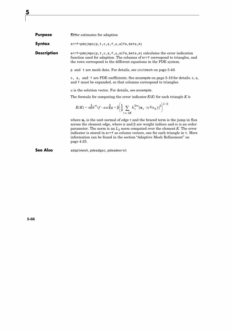
8/21/2019 matlab pde solving.pdf
http://slidepdf.com/reader/full/matlab-pde-solvingpdf 252/290
5-66
c, a, and f are PDE coefficients. See assempde on page 5-19 for details. c, a,
and f must be expanded, so that columns correspond to triangles.
u is the solution vector. For details, see assempde.
The formula for computing the error indicator E( K ) for each triangle K is
where nτ is the unit normal of edge τ and the braced term is the jump in fluxacross the element edge, where α and β are weight indices and m is an orderparameter. The norm is an L2 norm computed over the element K . The errorindicator is stored in errf as column vectors, one for each triangle in t. Moreinformation can be found in the section “Adaptive Mesh Refinement” onpage 4-25.
See Also adaptmesh, pdeadgsc, pdeadworst
E K ( ) α hm
f au – ( ) K = β12--- hτ
2mnτ[ c uh∇( ) ]
2⋅
τ ∂ K ∈
"# $% &' ( 1 2 ⁄
+
5pdemdlcvPurpose Convert PDE Toolbox 1.0 Model M-files to PDE Toolbox 1.0.2 format
Syntax pdemdlcv(infile,outfile)
Description pdemdlcv(infile,outfile) converts the PDE Toolbox 1.0 model -file infile to a PDE Toolbox 1.0.2 compatible model M-file. The resulting M-file is savedas outfile. If the .m extension is missing in outfile, it is added automatically.
If you want to use model M-files generated using PDE Toolbox 1.0, they mustfirst be converted using pdemdlcv.
8/21/2019 matlab pde solving.pdf
http://slidepdf.com/reader/full/matlab-pde-solvingpdf 253/290
5-67
first be converted using pdemdlcv.
Example pdedmdlcv('model42.m','model5.m') converts the PDE Toolbox 1.0 ModelM-file model42.m and saves the converted model in model5.m.
5
5pdemeshPurpose Plot a PDE triangular mesh
Syntax pdemesh(p,e,t)
pdemesh(p,e,t,u)
h=pdemesh(p,e,t)
h=pdemesh(p,e,t,u)
Description pdemesh(p,e,t) plots the mesh specified by the mesh data p, e, and t.
h d h( ) dditi ll t h dl t th l tt d bj t
8/21/2019 matlab pde solving.pdf
http://slidepdf.com/reader/full/matlab-pde-solvingpdf 254/290
5-68
h=pdemesh(p,e,t) additionally returns handles to the plotted axes objects.
pdemesh(p,e,t,u) plots PDE node or triangle data u using a mesh plot. If u isa column vector, node data is assumed. If u is a row vector, triangle data isassumed. This command plots substantially faster than the pdesurf command.
The geometry of the PDE problem is given by the mesh data p, e, and t. Fordetails on the mesh data representation, see initmesh on page 5-40.
This command is just shorthand for the calls
pdeplot(p,e,t)pdeplot(p,e,t,'zdata',u)
If you want to have more control over your mesh plot, use pdeplot instead ofpdemesh.
Examples Plot the mesh for the geometry of the L-shaped membrane.
[p,e,t]=initmesh('lshapeg');
[p,e,t]=refinemesh('lshapeg',p,e,t);pdemesh(p,e,t)
Now solve Poisson’s equation –∆u = 1 over the geometry defined by theL-shaped membrane. Use Dirichlet boundary conditions u = 0 on , and plotthe result.
u=assempde('lshapeb',p,e,t,1,0,1);
pdemesh(p,e,t,u)
See Also pdeplot, pdecont, pdesurf
Ω∂
5pdenonlinPurpose Solve nonlinear PDE problem
Syntax [u,res]=pdenonlin(b,p,e,t,c,a,f)
[u,res]=pdenonlin(b,p,e,t,c,a,f,'PropertyName',
'PropertyValue',...)
Description [u,res]=pdenonlin(b,p,e,t,c,a,f) solves the nonlinear PDE scalar PDEproblem
–∇ ⋅ (c∇u) + au = f on Ω
8/21/2019 matlab pde solving.pdf
http://slidepdf.com/reader/full/matlab-pde-solvingpdf 255/290
5-69
( ) f
or the nonlinear system PDE problem–∇ ⋅ (c ⊗ ∇u) + au = f on Ω
where the coefficients c, a, and f may depend on u. The algorithm solves theequation by using damped Newton iteration with the Armijo-Goldstein linesearch strategy.
The solution u is represented as the solution vector u. For details on therepresentation of the solution vector, see assempde on page 5-19. res is the
norm of the Newton step residuals.The triangular mesh of the PDE problem is given by the mesh data p, e, and t.For details on the mesh data representation, see initmesh on page 5-40.
b describes the boundary conditions of the PDE problem. b can be either aBoundary Condition matrix or the name of a Boundary M-file. The formats ofthe Boundary Condition matrix and Boundary M-file are described in theentries on assemb and pdebound, respectively, respectively. Note that for thegeneral call to pdebound the boundary conditions can also depend on u. Afixed-point iteration strategy is employed to solve for the nonlinear boundaryconditions.
The coefficients c, a, f of the PDE problem can be given in a wide variety ofways. In the context of pdenonlin the coefficients can depend on u. Thecoefficients cannot depend on t, the time. For a complete listing of all formatoptions, see assempde.
5
The solver can be fine-tuned by setting some of the options described below
Property Name Property Value Default Description
Jacobian f ixed|lumped|full fixed Approximation of Jacobian
U0 string or numeric 0 Initial solution guess
Tol positive scalar 1e 4 Residual size at termination
MaxIter positive integer 25 Maximum Gauss Newton
8/21/2019 matlab pde solving.pdf
http://slidepdf.com/reader/full/matlab-pde-solvingpdf 256/290
5-70
There are three methods currently implemented to compute the Jacobian:
•Numerical evaluation of the full Jacobian based on the sparse version of thefunction numjac
• A “lumped” approximation described in Chapter 4, “The Finite ElementMethod,” based on the numerical differentiation of the coefficients
• A fixed-point iteration matrix where the Jacobian is approximated by thestiffness matrix
Select the desired method by setting the Jacobian property to full, lumped, orfixed, bearing in mind that the more precise methods are computationallymore expensive.
U0 is the starting guess that can be given as an expression, a generic scalar, ora vector. By default it is set to 0, but this is useless in problems such as ∇(1/ u∇u) = 0 with Dirichlet boundary conditions u = e x+y. Tol fixes the exit criterionfrom the Gauss-Newton iteration, i.e., the iterations are terminated when the
residual norm is less than Tol. The norm in which the residual is computed isselected through Norm. This can be any admissible MATLAB vector norm orenergy for the energy norm.
MaxIter positive integer 25 Maximum Gauss-Newtoniterations
MinStep positive scalar 1/2^16 Minimum damping of searchdirection
Report on|off off Print convergence information
Norm string or numeric Inf Residual norm
MaxIter and MinStep are safeguards against infinite Gauss-Newton loops andthey bound the number of iterations and the step size used in each iteration.Setting Report to on forces printing of convergence information.
Diagnostics If the Newton iteration does not converge, the error message Too many
iterations or Stepsize too small is displayed. If the initial guess producesmatrices containing NaN or Inf elements, the error message Unsuitable
initial guess U0 (default: U0=0) is printed.
See Also assempde, pdebound
8/21/2019 matlab pde solving.pdf
http://slidepdf.com/reader/full/matlab-pde-solvingpdf 257/290
5-71
See Also assempde, pdebound
5
5pdeplotPurpose Generic PDE Toolbox plot function
Syntax pdeplot(p,e,t,'PropertyName',PropertyValue,)
h=pdeplot(p,e,t,'PropertyName',PropertyValue,)
Description pdeplot(p,e,t,p1,v1,...) is the generic PDE Toolbox plot function. It candisplay several functions of a PDE solution at the same time.
The geometry of the PDE problem is given by the mesh data p, e, and t. Fordetails on the mesh data representation, see initmesh on page 5-40.
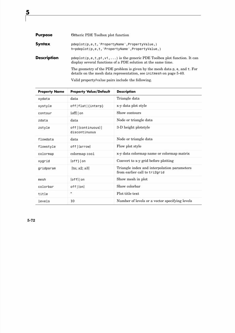
8/21/2019 matlab pde solving.pdf
http://slidepdf.com/reader/full/matlab-pde-solvingpdf 258/290
5-72
Valid property/value pairs include the following.
Property Name Property Value/Default Description
xydata data Triangle data
xystyle off|flat|interp x-y data plot style
contour off|on Show contours
zdata data Node or triangle data
zstyle off|continuous|discontinuous
3-D height plotstyle
flowdata data Node or triangle data
flowstyle off|arrow Flow plot style
colormap colormap cool x-y data colormap name or colormap matrix
xygrid off|on Convert to x-y grid before plotting
gridparam [tn; a2; a3] Triangle index and interpolation parametersfrom earlier call to tri2grid
mesh off|on Show mesh in plot
colorbar off|on Show colorbartitle ” Plot title text
levels 10 Number of levels or a vector specifying levels
The pdeplot is used both from inside the pdetool GUI and from the commandline. It is able to display three entities simultaneously. xydata can be visualized by a surface plot. Either flat or interpolated (default) shading can be
used for the surface plots. A contour plot can be superimposed on the surfaceplot (in black) or plotted independently (in colors) by setting contour to on.zdata is visualized by displaying height. The triangles can be either tilted byinterpolation (default) or flat. Flow data can be visualized by plotting arrowslike the MATLAB quiver plot. All data types can be either node data ortriangle data (flow data can only be triangle data). Node data is represented bya column vector of length size(p,2) and triangle data is represented by a row
8/21/2019 matlab pde solving.pdf
http://slidepdf.com/reader/full/matlab-pde-solvingpdf 259/290
5-73
vector of length size(t,2). If no xydata, zdata, or flowdata is supplied,pdeplot plots the mesh specified by p, e, and t.The option mesh displays or hides (default) the triangle mesh in the plot. Theoption xygrid first converts the data to x-y data (using tri2grid), and thenuses a standard MATLAB plotting algorithm. The property gridparam passesthe tri2grid data to pdeplot. This speeds up animation (see pdedemo5 andpdedemo6). The property colormap renders the plot using any MATLABcolormap or color matrix. colorbar adds a colorbar to the plot. title inserts atitle into the plot. levels only applies to contour plots: Given a scalar integer value, it plots that number of equally spaced contour levels; given a vector oflevel values, it plots those contour lines on the levels in the vector.
h=pdeplot(p,t,u) additionally returns handles to the drawn axes objects.
Examples The command sequence below plots the solution to Poisson's equation on theL-shaped membrane in 3-D.
[p,e,t]=initmesh('lshapeg');u=assempde('lshapeb',p,e,t,1,0,1);
pdeplot(p,e,t,'xydata',u,'zdata',u,'mesh','off');
See Also pdecont, pdegplot, pdemesh, pdesurf
5
5pdepolyPurpose Draw polygon
Syntax pdepoly(x,y)
pdepoly(x,y,label)
Description pdepoly(x,y) draws a polygon with corner coordinates defined by x and y. Ifthe pdetool GUI is not active, it is automatically started, and the polygon isdrawn in an empty geometry model.
The optional argument label assigns a name to the polygon (otherwise a

8/21/2019 matlab pde solving.pdf
http://slidepdf.com/reader/full/matlab-pde-solvingpdf 260/290
5-74
default name is chosen).
The state of the Geometry Description matrix inside pdetool is updated toinclude the polygon. You can export the Geometry Description matrix frompdetool by using the Export Geometry Description . . . option from the Draw menu. For a details on the format of the Geometry Description matrix, seedecsg on page 5-31.
Examples The command
pdepoly([ 1 0 0 1 1 1],[0 0 1 1 1 1]);
creates the L-shaped membrane geometry as one polygon.
See Also pdecirc, pderect, pdetool
5pdeprtniPurpose Interpolate from triangle midpoint data to node data
Syntax un=pdeprtni(p,t,ut)
Description un=pdeprtni(p,t,ut) gives linearly interpolated values at node points fromthe values at triangle midpoints.
The geometry of the PDE problem is given by the mesh data p and t. For detailson the mesh data representation, see initmesh on page 5-40.
Let N be the dimension of the PDE system, np the number of node points, and
8/21/2019 matlab pde solving.pdf
http://slidepdf.com/reader/full/matlab-pde-solvingpdf 261/290
5-75
Let N be the dimension of the PDE system, n p the number of node points, andn
t the number of triangles. The components of triangle data in ut are stored as
N rows of length nt. The components of the node data are stored in un as N columns of length n p.
Cautionary pdeprtni and pdeintrp are not inverse functions. The interpolation introducessome averaging.
See Also assempde, initmesh, pdeintrp
5
5pderectPurpose Draw rectangle
Syntax pderect(xy)
pderect(xy,label)
Description pderect(xy) draws a rectangle with corner coordinates defined by xy=[xmin
xmax ymin ymax]. If the pdetool GUI is not active, it is automatically started,and the rectangle is drawn in an empty geometry model.
The optional argument label assigns a name to the rectangle (otherwise ad f lt i h )
8/21/2019 matlab pde solving.pdf
http://slidepdf.com/reader/full/matlab-pde-solvingpdf 262/290
5-76
default name is chosen).
The state of the Geometry Description matrix inside pdetool is updated toinclude the rectangle. You can export the Geometry Description matrix frompdetool by selecting the Export Geometry Description . . . option from theDraw menu. For details on the format of the Geometry Description matrix, seedecsg on page 5-31.
Examples The command sequence below starts pdetool and draws the L-shapedmembrane as the union of three squares.
pderect([ 1 0 1 0])
pderect([0 1 1 0])
pderect([0 1 0 1])
See Also pdecirc, pdeellip, pdepoly, pdetool
5pdesdp, pdesde, pdesdtPurpose Indices of points/edges/triangles in a set of subdomains
Syntax c=pdesdp(p,e,t)
[i,c]=pdesdp(p,e,t)
c=pdesdp(p,e,t,sdl)
[i,c]=pdesdp(p,e,t,sdl)
i=pdesdt(t)
i=pdesdt(t,sdl)
i=pdesde(e)
i=pdesde(e sdl)
8/21/2019 matlab pde solving.pdf
http://slidepdf.com/reader/full/matlab-pde-solvingpdf 263/290
5-77
i=pdesde(e,sdl)
Description [i,c]=pdesdp(p,e,t,sdl) given mesh data p, e, and t and a list of subdomainnumbers sdl, the function returns all points belonging to those subdomains. Apoint can belong to several subdomains, and the points belonging to thedomains in sdl are divided into two disjoint sets. i contains indices of thepoints that wholly belong to the subdomains listed in sdl, and c lists pointsthat also belongs to the other subdomains.
c=pdesdp(p,e,t,sdl) returns indices of points that belong to more than one ofthe subdomains in sdl.
i=pdesdt(t,sdl) given triangle data t and a list of subdomain numbers sdl,i contains indices of the triangles inside that set of subdomains.
i=pdesde(e,sdl) given edge data e, it extracts indices of outer boundary edgesof the set of subdomains.
If sdl is not given, a list of all subdomains is assumed.
5
5pdesmechPurpose Calculate structural mechanics tensor functions
Syntax ux=pdesmech(p,t,c,u,'PropertyName',PropertyValue,...)
Description ux=pdesmech(p,t,c,u,p1,v1,...) returns a tensor expression evaluated atthe center of each triangle. The tensor expressions are stresses and strains forstructural mechanics applications with plane stress or plane strain conditions.pdesmech is intended to be used for postprocessing of a solution computed usingthe structural mechanics application modes of the pdetool GUI, afterexporting the solution, the mesh, and the PDE coefficients to the MATLAB

8/21/2019 matlab pde solving.pdf
http://slidepdf.com/reader/full/matlab-pde-solvingpdf 264/290
5-78
main workspace. Poisson’s ratio, nu, has to be supplied explicitly forcalculations of shear stresses and strains, and for the von Mises effective stressin plane strain mode.
Valid property name/property value pairs include the following.
The available tensor expressions are
•
•
•
•
• exx, the x-direction strain (ε x)
• eyy, the y-direction strain (ε y)
• exy, the shear strain (γ xy)
• sxx, the x-direction stress (σ x)• syy, the y-direction stress (σ y)
• sxy, the shear stress (τ xy)
Property Name Property Value/Default Description
tensor ux|uy|vx|vy|exx|eyy|exy|sxx|syy|sxy|e1|
e2|s1|s2|von Mises
Tensor expression
application ps|pn Plane stress|plane strain
nu Scalar or string expression 0.3 Poisson’s ratio
ux ∂u
∂ x
------=
uy ∂u∂ y------=
vx ∂v
∂ x------=
vy ∂v
∂ y------=
• e1, the first principal strain (ε1)
• e2, the second principal strain (ε2)
•s1, the first principal stress (σ1)
• s2, the second principal stress (σ2)
• von Mises, the von Mises effective stress, for plane stress conditions
or for plane strain conditions
σ12
σ22
σ1σ2 – +
8/21/2019 matlab pde solving.pdf
http://slidepdf.com/reader/full/matlab-pde-solvingpdf 265/290
5-79
Examples Assuming that a problem has been solved using the application mode“Structural Mechanics, Plane Stress,” discussed in “Structural Mechanics —Plane Stress” on page 2-38, and that the solution u, the mesh data p and t, andthe PDE coefficient c all have been exported to the MATLAB main workspace,the x-direction strain is computed as
sx=pdesmech(p,t,c,u,'tensor','sxx');
To compute the von Mises effective stress for a plane strain problem withPoisson’s ratio equal to 0.3, type
mises=pdesmech(p,t,c,u,'tensor','von Mises',...
'application','pn','nu',0.3);
σ12 σ22+( ) v2 v – 1+( ) σ1σ2 2v2 2v – 1 – ( ) –
5
5pdesurf Purpose Shorthand command for surface plot
Syntax pdesurf(p,t,u)
Description pdesurf(p,t,u) plots a 3-D surface of PDE node or triangle data. If u is acolumn vector, node data is assumed, and continuous style and interpolatedshading are used. If u is a row vector, triangle data is assumed, anddiscontinuous style and flat shading are used.
h=pdesurf(p,t,u) additionally returns handles to the drawn axes objects.

8/21/2019 matlab pde solving.pdf
http://slidepdf.com/reader/full/matlab-pde-solvingpdf 266/290
5-80
For node data, this command is just shorthand for the callpdeplot(p,[],t,'xydata',u,'xystyle','interp',...
'zdata',u,'zstyle','continuous','colorbar','off');
and for triangle data it is
pdeplot(p,[],t,'xydata',u,'xystyle','flat',...
'zdata',u,'zstyle','discontinuous','colorbar','off');
If you want to have more control over your surface plot, use pdeplot instead ofpdesurf.
Examples Surface plot of the solution to the equation –∆u = 1 over the geometry definedby the L-shaped membrane. Use Dirichlet boundary conditions u = 0 on .
[p,e,t]=initmesh('lshapeg');
[p,e,t]=refinemesh('lshapeg',p,e,t);
u=assempde('lshapeb',p,e,t,1,0,1);
pdesurf(p,t,u)
See Also pdeplot, pdecont, pdemesh
Ω∂
5pdetoolPurpose PDE Toolbox graphical user interface (GUI)
Syntax pdetool
pdetool(action,flag)
Description pdetool provides the graphical user interface (GUI) for the PDE Toolbox. Callpdetool without arguments to start the application. You should not callpdetool with arguments.
The GUI helps you to draw the 2-D domain and to define boundary conditionsfor a PDE problem It also makes it possible to specify the partial differential
8/21/2019 matlab pde solving.pdf
http://slidepdf.com/reader/full/matlab-pde-solvingpdf 267/290
5-81
for a PDE problem. It also makes it possible to specify the partial differential
equation, to create, inspect and refine the mesh, and to compute and displaythe solution from the GUI.
pdetool contains several different modes:
In Draw mode, you construct a Constructive Solid Geometry model (CSGmodel) of the geometry. You can draw solid objects that can overlap. There arefour types of solid objects:
•Circle object — represents the set of points inside a circle.
•Polygon object — represents the set of points inside the polygon given by aset of line segments.
•Rectangle object — represents the set of points inside the rectangle given bya set of line segments.
•Ellipse object — represents the set of points inside an ellipse. The ellipse canbe rotated.
The solid objects can be moved and rotated. Operations apply to groups ofobjects by doing multiple selects. (A Select all option is also available.) You cancut and paste among the selected objects. The model can be saved and restored.pdetool can be started by just typing the name of the model. (This starts thecorresponding M-file that contains the MATLAB commands necessary tocreate the model.)
The solid objects can be combined by typing a set formula. Each object isautomatically assigned a unique name, which is displayed in the GUI on thesolid object itself. The names refer to the object in the set formula. Morespecifically, in the set formula, the name refers to the set of points inside theobject. The resulting geometrical model is the set of points for which the setformula evaluates to true. (For a description of the syntax of the set formula,
5
see decsg.) By default, the resulting geometrical model is the union of allobjects.
A “snap-to-grid” function is available. This means that objects align to the grid.The grid can be turned on and off, and the scaling and the grid spacing can bechanged.
In boundary mode, you can specify the boundary conditions. You can havedifferent types of boundary conditions on different boundaries. In this mode,the original shapes of the solid building objects constitute borders betweensubdomains of the model. Such borders can be eliminated in this mode. Theouter boundaries are color coded to indicate the type of boundary conditions A
8/21/2019 matlab pde solving.pdf
http://slidepdf.com/reader/full/matlab-pde-solvingpdf 268/290
5-82
outer boundaries are color coded to indicate the type of boundary conditions. A
red outer boundary corresponds to Dirichlet boundary conditions, blue togeneralized Neumann boundary conditions, and green to mixed boundaryconditions. You can return to the boundary condition display by clicking the
button or by selecting Boundary Mode from the Boundary menu.
In PDE mode, you can specify the type of PDE problem, and the coefficients c,
a, f, and d. You can specify the coefficients for each subdomain independently.This makes it easy to specify, e.g., various material properties in one PDEmodel. The PDE to be solved can be specified by clicking the PDE button or byselecting PDE Specification . . . from the PDE menu. This brings up a dialogbox.
In Mesh mode, you can control the automated mesh generation and plot themesh. An initial mesh can be generated by clicking the button or byselecting Initialize Mesh from the Mesh menu. The initial mesh can berepeatedly refined by clicking the refine button or by selecting Refine Mesh from the Mesh menu.
In Solve mode, you can specify solve parameters and solve the PDE. Forparabolic and hyperbolic PDE problems, you can also specify the initialconditions, and the times at which the output should be generated. Foreigenvalue problems, the search range can be specified. Also, the adaptive andnonlinear solvers for elliptic PDEs can be invoked. The PDE problem is solvedby clicking the = button or by selecting Solve PDE from the Solve menu. Bydefault, the solution is plotted in the pdetool axes.
∂Ω
In Plot mode you can select a wide variety of visualization methods such assurface, mesh, contour, and quiver (vector field) plots. For surface plots, youcan choose between interpolated and flat rendering schemes. The mesh can be
hidden in all plot types. For parabolic and hyperbolic equations, you cananimate the solution as it changes with time. You can show the solution bothin 2-D and 3-D. 2-D plots are shown inside pdetool. 3-D plots are plotted inseparate figure windows. Different types of plots can be selected by clicking thebutton with the solution plot icon or by selecting Parameters . . . from the Plot menu. This opens a dialog box.
Boundary Condition Dialog Box
8/21/2019 matlab pde solving.pdf
http://slidepdf.com/reader/full/matlab-pde-solvingpdf 269/290
5-83
Boundary Condition Dialog Box
In this dialog box, the boundary condition for the selected boundaries isentered.The following boundary conditions can be handled:
• Dirichlet: hu = r on the boundary.
•Generalized Neumann: on the boundary.
• Mixed: a combination of Dirichlet and generalized Neumann condition.
is the outward unit length normal.
The boundary conditions can be entered in a variety of ways. (See assemb onpage 5-15 and “Boundary Menu” on page 3-13.)
PDE Specification Dialog Box In this dialog box, the type of PDE and the PDE coefficients are entered. Thefollowing types of PDEs can be handled:
•
Elliptic PDE: –∇ ⋅
(c∇u
) + au
= f
•Parabolic PDE:
•Hyperbolic PDE:
•Eigenvalue PDE: –∇ ⋅ (c∇u) + au = λdu
for x and y on the problem’s 2-D domain Ω.
The PDE coefficients can be entered in a variety of ways. (See assempde onpage 5-19 and “PDE Menu” on page 3-16.)
n c∇u( ) qu+⋅ g=
n
d∂u
∂t------ ∇ c∇u( ) au+⋅ – f =
d∂
2u
∂t2
--------- ∇ c∇u( ) au+⋅ – f =
5
Model M-FileThe Model M-file contains the MATLAB commands necessary to create a CSGmodel. It can also contain additional commands to set boundary conditions,define the PDE, create the mesh, solve the pde, and plot the solution. This typeof M-file can be saved and opened from the File menu.
The Model M-file is a MATLAB function and not a script. This way nameclashes between variables used in the function and in the main workspace areavoided. The name of the file must coincide with the model name. Thebeginning of the file always looks similar to the code fragment below:
function pdemodel
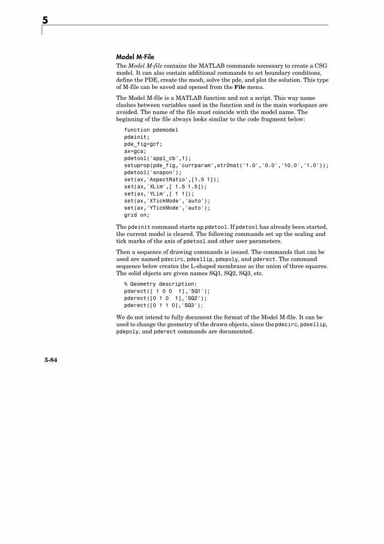
8/21/2019 matlab pde solving.pdf
http://slidepdf.com/reader/full/matlab-pde-solvingpdf 270/290
5-84
function pdemodel
pdeinit;
pde_fig=gcf;
ax=gca;
pdetool('appl_cb',1);
setuprop(pde_fig,'currparam',str2mat('1.0','0.0','10.0','1.0'));
pdetool('snapon');
set(ax,'AspectRatio',[1.5 1]);
set(ax,'XLim',[ 1.5 1.5]);
set(ax,'YLim',[ 1 1]);set(ax,'XTickMode','auto');
set(ax,'YTickMode','auto');
grid on;
The pdeinit command starts up pdetool. If pdetool has already been started,the current model is cleared. The following commands set up the scaling andtick marks of the axis of pdetool and other user parameters.
Then a sequence of drawing commands is issued. The commands that can beused are named pdecirc, pdeellip, pdepoly, and pderect. The commandsequence below creates the L-shaped membrane as the union of three squares.The solid objects are given names SQ1, SQ2, SQ3, etc.
% Geometry description:
pderect([ 1 0 0 1],'SQ1');
pderect([0 1 0 1],'SQ2');
pderect([0 1 1 0],'SQ3');
We do not intend to fully document the format of the Model M-file. It can beused to change the geometry of the drawn objects, since the pdecirc, pdeellip,pdepoly, and pderect commands are documented.
See Also initmesh, assempde, parabolic, wave, pdeeig, pdesurf, pdecont
8/21/2019 matlab pde solving.pdf
http://slidepdf.com/reader/full/matlab-pde-solvingpdf 271/290
5-85
5
5pdetrgPurpose Triangle geometry data
Syntax [ar,a1,a2,a3]=pdetrg(p,t)
[ar,g1x,g1y,g2x,g2y,g3x,g3y]=pdetrg(p,t)
Description [ar,a1,a2,a3]=pdetrg(p,t) returns the area of each triangle in ar and halfof the negative cotangent of each angle in a1, a2, and a3.
[ar,g1x,g1y,g2x,g2y,g3x,g3y]=pdetrg(p,t) returns the area and thegradient components of the triangle base functions.
8/21/2019 matlab pde solving.pdf
http://slidepdf.com/reader/full/matlab-pde-solvingpdf 272/290
5-86
The triangular mesh of the PDE problem is given by the mesh data p and t.For details on the mesh data representation, see initmesh on page 5-40.
5pdetriqPurpose Triangle quality measure
Syntax q=pdetriq(p,t)
Description q=pdetriq(p,t) returns a triangle quality measure given mesh data.
The triangular mesh is given by the mesh data p, e, and t. For details on themesh data representation, see initmesh on page 5-40.
The triangle quality is given by the formula
4 3a

8/21/2019 matlab pde solving.pdf
http://slidepdf.com/reader/full/matlab-pde-solvingpdf 273/290
5-87
where a is the area and h1, h2, and h3 the side lengths of the triangle.
If q > 0.6 the triangle is of acceptable quality. q = 1 when h1 = h2 = h3.
See Also initmesh, jigglemesh, refinemesh
Reference Bank, Randolph E., PLTMG: A Software Package for Solving Elliptic Partial Differential Equations, User’s Guide 6.0, Society for Industrial and AppliedMathematics, Philadelphia, PA, 1990.
q
4 3a
h12 h2
2 h32+ +--------------------------------=
5
5poiasmaPurpose Boundary point matrix contributions for fast solvers of Poisson’s equation
Syntax K=poiasma(n1,n2,h1,h2)
K=poiasma(n1,n2)
K=poiasma(n)
Description K=poiasma(n1,n2,h1,h2) assembles the contributions to the stiffness matrixfrom boundary points. n1 and n2 are the numbers of points in the first andsecond directions, and h1 and h2 are the mesh spacings. K is a sparsen1*n2-by-n1*n2 matrix. The point numbering is the canonical numbering for arectangular mesh
8/21/2019 matlab pde solving.pdf
http://slidepdf.com/reader/full/matlab-pde-solvingpdf 274/290
5-88
rectangular mesh.
K=poiasma(n1,n2) uses h1=h2.
K=poiasma(n) uses n1=n2=n.
See Also poiindex, poisolv
5poicalcPurpose Fast solver for Poisson’s equation on a rectangular grid
Syntax u=poicalc(f,h1,h2,n1,n2)
u=poicalc(f,h1,h2)
u=poicalc(f)
Description u=poicalc(f,h1,h2,n1,n2) calculates the solution of Poisson’s equation forthe interior points of an evenly spaced rectangular grid. The columns of u contain the solutions corresponding to the columns of the right-hand side f. h1 and h2 are the spacings in the first and second direction, and n1 and n2 are thenumber of points
8/21/2019 matlab pde solving.pdf
http://slidepdf.com/reader/full/matlab-pde-solvingpdf 275/290
5-89
number of points.
The number of rows in f must be n1*n2. If n1 and n2 are not given, the squareroot of the number of rows of f is assumed. If h1 and h2 are not given, they areassumed to be equal.
The ordering of the rows in u and f is the canonical ordering of interior points,as returned by poiindex.
The solution is obtained by sine transforms in the first direction and
tridiagonal matrix solution in the second direction. n1 should be 1 less than apower of 2 for best performance.
See Also poiindex, poiasma, dst, idst, poisolv
5
5poiindexPurpose Indices of points in canonical ordering for rectangular grid
Syntax [n1,n2,h1,h2,i,c,ii,cc]=poiindex(p,e,t,sd)
Description [n1,n2,h1,h2,i,c,ii,cc]=poiindex(p,e,t,sd) identifies a given grid p, e, tin the subdomain sd as an evenly spaced rectangular grid. If the grid is notrectangular, n1 is 0 on return. Otherwise n1 and n2 are the number of points inthe first and second directions, h1 and h2 are the spacings. i and ii are oflength (n1 2)*(n2 2) and contain indices of interior points. i contains indicesof the original mesh, whereas ii contains indices of the canonical ordering. c and cc are of length n1*n2 (n1 2)*(n2 2) and contain indices of border
8/21/2019 matlab pde solving.pdf
http://slidepdf.com/reader/full/matlab-pde-solvingpdf 276/290
5-90
g ( ) ( )
points. ii and cc are increasing.In the canonical ordering, points are numbered from “left to right” and thenfrom “bottom to top.” Thus if n1=3 and n2=5, then ii=[5 8 11] andcc=[1 2 3 4 6 7 9 10 12 13 14 15].
See Also poisolv, poiasma
5poimeshPurpose Make regular mesh on a rectangular geometry
Syntax [p,e,t]=poimesh(g,nx,ny)
[p,e,t]=poimesh(g,n)
[p,e,t]=poimesh(g)
Description [p,e,t]=poimesh(g,nx,ny) constructs a regular mesh on the rectangulargeometry specified by g, by dividing the “x edge” into nx pieces and the “y edge”into ny pieces, and placing (nx+1)*(ny+1) points at the intersections.
The “x edge” is the one that makes the smallest angle with the x-axis.
8/21/2019 matlab pde solving.pdf
http://slidepdf.com/reader/full/matlab-pde-solvingpdf 277/290
5-91
[p,e,t]=poimesh(g,n) uses nx=ny=n, and [p,e,t]=poimesh(g) uses nx=ny=1.
The triangular mesh is described by the mesh data p, e, and t. For details onthe mesh data representation, see initmesh on page 5-40.
For best performance with poisolv, the larger of nx and ny should be a powerof 2.
If g does not seem to describe a rectangle, p is zero on return.
Examples Try the demo command pdedemo8. The solution of Poisson’s equation over arectangular grid with boundary condition given by the file squareb4 isreturned. The solution time is compared to the usual Finite Element Method(FEM) approach.
See Also initmesh, poisolv
5
5poisolvPurpose Fast solution of Poisson’s equation on a rectangular grid
Syntax u=poisolv(b,p,e,t,f)
Description u=poisolv(b,p,e,t,f) solves Poisson’s equation with Dirichlet boundaryconditions on a regular rectangular grid. A combination of sine transforms andtridiagonal solutions is used for increased performance.
The boundary conditions b must specify Dirichlet conditions for all boundarypoints.
The mesh p, e, and t must be a regular rectangular grid. For details on the
8/21/2019 matlab pde solving.pdf
http://slidepdf.com/reader/full/matlab-pde-solvingpdf 278/290
5-92
p, , g g gmesh data representation, see initmesh on page 5-40.
f gives the right-hand side of Poisson’s equation.
Apart from roundoff errors, the result should be the same asu=assempde(b,p,e,t,1,0,f).
See Also poicalc, poimesh
Reference Strang, Gilbert, Introduction to Applied Mathematics, Wellesley-CambridgePress, Cambridge, MA, 1986, pp. 453–458.
5refinemeshPurpose Refine a triangular mesh
Syntax [p1,e1,t1]=refinemesh(g,p,e,t)
[p1,e1,t1]=refinemesh(g,p,e,t,'regular')
[p1,e1,t1]=refinemesh(g,p,e,t,'longest')
[p1,e1,t1]=refinemesh(g,p,e,t,it)
[p1,e1,t1]=refinemesh(g,p,e,t,it,'regular')
[p1,e1,t1]=refinemesh(g,p,e,t,it,'longest')
[p1,e1,t1,u1]=refinemesh(g,p,e,t,u)
[p1,e1,t1,u1]=refinemesh(g,p,e,t,u,'regular')
8/21/2019 matlab pde solving.pdf
http://slidepdf.com/reader/full/matlab-pde-solvingpdf 279/290
5-93
[p1,e1,t1,u1]=refinemesh(g,p,e,t,u,'longest')[p1,e1,t1,u1]=refinemesh(g,p,e,t,u,it)
[p1,e1,t1,u1]=refinemesh(g,p,e,t,u,it,'regular')
[p1,e1,t1,u1]=refinemesh(g,p,e,t,u,it,'longest')
Description [p1,e1,t1]=refinemesh(g,p,e,t) returns a refined version of the triangularmesh specified by the geometry g, Point matrix p, Edge matrix e, and Trianglematrix t.
The triangular mesh is given by the mesh data p, e, and t. For details on themesh data representation, see initmesh on page 5-40.
[p1,e1,t1,u1]=refinemesh(g,p,e,t,u) refines the mesh and also extendsthe function u to the new mesh by linear interpolation. The number of rows inu should correspond to the number of columns in p, and u1 has as many rowsas there are points in p1. Each column of u is interpolated separately.
An extra input argument it is interpreted as a list of subdomains to refine, ifit is a row vector, or a list of triangles to refine, if it is a column vector.
The default refinement method is regular refinement, where all of the specifiedtriangles are divided into four triangles of the same shape. Longest edgerefinement, where the longest edge of each specified triangle is bisected, can bedemanded by giving longest as a final parameter. Using regular as a finalparameter results in regular refinement. Some triangles outside of thespecified set may also be refined, in order to preserve the triangulation and its
quality.
Examples Refine the mesh of the L-shaped membrane several times. Plot the mesh for thegeometry of the L-shaped membrane.
5
[p,e,t]=initmesh('lshapeg','hmax',inf);
subplot(2,2,1), pdemesh(p,e,t)
[p,e,t]=refinemesh('lshapeg',p,e,t);
subplot(2,2,2), pdemesh(p,e,t)[p,e,t]=refinemesh('lshapeg',p,e,t);
subplot(2,2,3), pdemesh(p,e,t)
[p,e,t]=refinemesh('lshapeg',p,e,t);
subplot(2,2,4), pdemesh(p,e,t)
subplot
Algorithm The algorithm is described by the steps below:
8/21/2019 matlab pde solving.pdf
http://slidepdf.com/reader/full/matlab-pde-solvingpdf 280/290
5-94
1 Pick the initial set of triangles to be refined.
2 Either divide all edges of the selected triangles in half (regular refinement),or divide the longest edge in half (longest edge refinement).
3 Divide the longest edge of any triangle that has a divided edge.
4 Repeat step 3 until no further edges are divided.
5 Introduce new points of all divided edges, and replace all divided entries ine by two new entries.
6 Form the new triangles. If all three sides are divided, new triangles areformed by joining the side midpoints. If two sides are divided, the midpointof the longest edge is joined with the the opposing corner and with the othermidpoint. If only the longest edge is divided, its midpoint is joined with the
opposing corner.
See Also initmesh, pdegeom, pdesdt, pdeent
5sptarnPurpose Solve generalized sparse eigenvalue problem
Syntax [xv,lmb,iresult] = sptarn(A,B,lb,ub)
[xv,lmb,iresult] = sptarn(A,B,lb,ub,spd)
[xv,lmb,iresult] = sptarn(A,B,lb,ub,spd,tolconv)
[xv,lmb,iresult] = sptarn(A,B,lb,ub,spd,tolconv,jmax)
[xv,lmb,iresult] = sptarn(A,B,lb,ub,spd,tolconv,jmax,maxmul)
Description [xv,lmb,iresult] = sptarn(A,B,lb,ub,spd,tolconv,jmax,maxmul) findseigenvalues of the pencil ( A – λ B) x = 0 in interval [lb,ub]. (A matrix of linearpolynomials A – λ B , A – λ B, is called a pencil.)
8/21/2019 matlab pde solving.pdf
http://slidepdf.com/reader/full/matlab-pde-solvingpdf 281/290
5-95
p yij ij
, , p
A and B are sparse matrices. lb and ub are lower and upper bounds foreigenvalues to be sought. We may have lb= inf if all eigenvalues to the left ofub are sought, and rb=inf if all eigenvalues to the right of lb are sought. Oneof lb and ub must be finite. A narrower interval makes the algorithm faster. Inthe complex case, the real parts of lmb are compared to lb and ub.
xv are eigenvectors, ordered so that norm(a*xv b*xv*diag(lmb)) is small. lmb
is the sorted eigenvalues. If iresult>=0 the algorithm succeeded, and alleigenvalues in the intervals have been found. If iresult<0 the algorithm hasnot yet been successful, there may be more eigenvalues — try with a smallerinterval.
spd is 1 if the pencil is known to be symmetric positive definite (default 0).
tolconv is the expected relative accuracy. Default is 100*eps, where eps is themachine precision.
jmax is the maximum number of basis vectors. The algorithm needs jmax*n working space so a small value may be justified on a small computer, otherwiselet it be the default value jmax=100. Normally the algorithm stops earlier whenenough eigenvalues have converged.
maxmul is the number of Arnoldi runs tried. Must at least be as large asmaximum multiplicity of any eigenvalue. If a small value of jmax is given,
many Arnoldi runs are necessary. The default value ismaxmul=n
, which isneeded when all the eigenvalues of the unit matrix are sought.
Algorithm The Arnoldi algorithm with spectral transformation is used. The shift is chosenat ub, lb, or at a random point in interval (lb,ub) when both bounds are finite.
5
The number of steps j in the Arnoldi run depends on how many eigenvaluesthere are in the interval, but it stops at j=min(jmax,n). After a stop, thealgorithm restarts to find more Schur vectors in orthogonal complement to all
those already found. When no more eigenvalues are found in lb < lmb <= ub,the algorithm stops. For small values of jmax, several restarts may be neededbefore a certain eigenvalue has converged. The algorithm works when jmax isat least one larger than the number of eigenvalues in the interval, but thenmany restarts are needed. For large values of jmax, which is the preferredchoice, mul+1 runs are needed. mul is the maximum multiplicity of aneigenvalue in the interval.
8/21/2019 matlab pde solving.pdf
http://slidepdf.com/reader/full/matlab-pde-solvingpdf 282/290
5-96
Note The algorithm works on nonsymmetric as well as symmetric pencils,but then accuracy is approximately tol times the Henrici departure fromnormality. The parameter spd is used only to choose between symmmd andcolmmd when factorizing, the former being marginally better for symmetricmatrices close to the lower end of the spectrum.
In case of trouble,
If convergence is too slow, try (in this order of priority): a smaller interval lb, ub a larger jmax
a larger maxmul
If factorization fails, try again with lb or ub finite. Then shift is chosen atrandom and hopefully not at an eigenvalue. If it fails again, check whether
pencil may be singular.If it goes on forever, there may be too many eigenvalues in the strip. Try witha small value maxmul=2 and see which eigenvalues you get. Those you get aresome of the eigenvalues, but a negative iresult tells you that you have notgotten them all.
If memory overflow, try smaller jmax.
The algorithm is designed for eigenvalues close to the real axis. If you wantthose close to the imaginary axis, try A=i*A.
When spd=1, the shift is at lb so that advantage is taken of the fasterfactorization for symmetric positive definite matrices. No harm is done, but
the execution is slower if lb is above the lowest eigenvalue.
See Also pdeeig
Reference Golub, Gene H., and Charles F. Van Loan, Matrix Computations, 2nd edition,Johns Hopkins University Press, Baltimore, MD, 1989.
8/21/2019 matlab pde solving.pdf
http://slidepdf.com/reader/full/matlab-pde-solvingpdf 283/290
5-97
Saad, Yousef, “Variations on Arnoldi’s Method for Computing Eigenelementsof Large Unsymmetric Matrices,” Linear Algebra and its Applications, Vol. 34,1980, pp. 269–295.
5
5tri2gridPurpose Interpolate from PDE triangular mesh to rectangular grid
Syntax uxy=tri2grid(p,t,u,x,y)
[uxy,tn,a2,a3]=tri2grid(p,t,u,x,y)
uxy=tri2grid(p,t,u,tn,a2,a3)
Description uxy=tri2grid(p,t,u,x,y) computes the function values uxy over the griddefined by the vectors x and y, from the function u with values on the triangularmesh defined by p and t. Values are computed using linear interpolation in thetriangle containing the grid point. The vectors x and y must be increasing.
8/21/2019 matlab pde solving.pdf
http://slidepdf.com/reader/full/matlab-pde-solvingpdf 284/290
5-98
[uxy,tn,a2,a3]=tri2grid(p,t,u,x,y) additionally lists the index tn of thetriangle containing each grid point, and interpolation coefficients a2 and a3.
uxy=tri2grid(p,t,u,tn,a2,a3) , with tn, a2, and a3 computed in an earliercall to tri2grid, interpolates using the same grid as in the earlier call. This variant is, however, much faster if several functions have to be interpolatedusing the same grid.
For grid points outside of the triangular mesh, NaN is returned in uxy, tn, a2,and a3.
See Also initmesh, refinemesh, assempde
5wboundPurpose Write boundary condition specification file
Syntax fid=wbound(bl,mn)
Description fid=wbound(bl,mn) writes a Boundary M-file with the name [mn,'.m']. TheBoundary M-file is equivalent to the Boundary Condition matrix bl. fid returns –1 if the file could not be written.
bl describes the boundary conditions of the PDE problem. bl is a BoundaryCondition matrix. For details, see assemb on page 5-15.
[mn,'.m'] pdebound

8/21/2019 matlab pde solving.pdf
http://slidepdf.com/reader/full/matlab-pde-solvingpdf 285/290
5-99
The output file is the name of a Boundary M-file. (See onpage 5-50.)
See Also decsg, pdegeom, pdebound, wgeom
5
5wgeomPurpose Write geometry specification function
Syntax fid=wgeom(dl,mn)
Description fid=wgeom(dl,mn) writes a Geometry M-file with the name [mn,'.m']. TheGeometry M-file is equivalent to the Decomposed Geometry matrix dl. fid returns –1 if the file could not be written.
dl is a Decomposed Geometry matrix. For a description of the format of theDecomposed Geometry matrix, see decsg on page 5-31.
[mn,'.m']
8/21/2019 matlab pde solving.pdf
http://slidepdf.com/reader/full/matlab-pde-solvingpdf 286/290
5-100
The output file is the name of a Geometry M-file. For a descriptionof the Geometry M-file format, see pdegeom on page 5-60.
See Also decsg, pdegeom, wbound
Index
A AC power electromagnetics 2-53adaptive mesh refinement 1-24
adaptmesh function 5-9animation 2-19 Application command 3-9application modes 2-37 Armijo-Goldstein line search 4-21 Arnoldi algorithm 5-95assema function 5-14assemb function 5-15
csgchk function 5-29csgdel function 5-30
cylindrical problem 2-21
Ddecomposed geometry 1-30Decomposed Geometry matrix 1-42decsg function 5-31discrete sine transform 4-28
8/21/2019 matlab pde solving.pdf
http://slidepdf.com/reader/full/matlab-pde-solvingpdf 287/290
I-1
assembling 4-6assempde function 5-19 Axes Limits command 3-9
BBoolean table 5-31
border segment 5-33boundary condition 3-14, 5-15Boundary Condition matrix 1-42Boundary menu 3-13Boundary M-file 1-42boundary mode 1-29boundary segment 5-33
Ccircle solid 5-32Coefficient matrix 1-43Coefficient M-file 1-43command-line functions, using 1-40conductive media DC 2-59Constructive Solid Geometry model 1-30CSG model 1-30
domain decomposition 2-13Draw menu 3-10draw mode 1-29dst function 5-36
E
Edge matrix 1-43Edit menu 3-5eigenmodes 2-34eigenvalue equation 4-16eigenvalue problems 1-24eigenvector matrix 5-55electrostatics 2-44ellipse solid 5-33
elliptic equation 1-3elliptic problems 2-2elliptic system 4-9energy norm 4-5
Ffast solver 4-28FEM 1-20File menu 3-2Finite Element Method 4-1
Index
GGauss-Newton method 4-21Geometry Description matrix 1-42
Geometry M-file 1-42graphical user interface, using 1-9Green’s formula 1-22Grid Spacing command 3-8
Hheat distribution in radioactive rod 2-21
h i 2 17
mesh data 1-43Mesh menu 3-20mesh mode 1-29
mesh parameters 3-21method of lines 4-13minimal region 1-42minimal surface problem 2-11Model M-file 1-39
NN S i 1 42
8/21/2019 matlab pde solving.pdf
http://slidepdf.com/reader/full/matlab-pde-solvingpdf 288/290
I-2
heat equation 2-17heat transfer 2-62Helmholtz’s equation 2-7Help menu 3-35hyperbolic equation 1-3hyperbolic function 5-37hyperbolic problems 2-23
Iinitmesh function 5-40
Jjigglemesh function 5-44
L Laplace equation 2-45L-shaped membrane 2-28
Mmagnetostatics 2-47mass matrix 4-5Maxwell’s equations 2-44menus 1-26
Name Space matrix 1-42New command 3-2node data 5-65nonlinear equation 4-20nonlinear problem 2-11nonlinear solver 1-24
OOpen command 3-3Options menu 3-7
Pparabolic equation 1-3
parabolic function 5-45parabolic problems 2-17Paste command 3-6PDE coefficients 3-17PDE menu 3-16PDE mode 1-29PDE Specification 3-17pdeadgsc function 5-47pdeadworst function 5-48pdearcl function 5-49pdebound function 5-50
Index
pdecgrad function 5-52pdecirc function 5-53pdecont function 5-54
pdeeig function 5-55pdeellip function 5-58pdegeom function 5-60pdegplot function 5-63pdegrad function 5-64pdeintrp function 5-65pdejmps function 5-66pdemdlcv function 5-67d h f ti 5 68
Poisson’s equation 1-9polygon solid 5-32Print command 3-4
R rectangle solid 5-32refinemesh function 5-93Robin boundary condition 4-2Rotate command 3-12
8/21/2019 matlab pde solving.pdf
http://slidepdf.com/reader/full/matlab-pde-solvingpdf 289/290
I-3
pdemesh function 5-68pdenonlin function 5-69pdeplot function 5-72pdepoly function 5-74pdeprtni function 5-75pderect function 5-76pdesde function 5-77
pdesdp function 5-77pdesdt function 5-77pdesmech function 5-78pdesurf function 5-80pdetool function 5-81pdetrg function 5-86pdetriq function 5-87pencil 5-95plane strain 2-44plane stress 2-38Plot menu 3-28plot mode 1-29Plot parameters 3-29poiasma function 5-88poicalc function 5-89
poiindex function 5-90poimesh function 5-91Point matrix 1-43poisolv function 5-92
SSave As command 3-3scattering problem 2-7Schur vector 4-18set formula 1-5skin effect 2-55
solid object 1-10solution vector 1-43Solve menu 3-23solve mode 1-29solve parameters 3-24sptarn function 5-95stiff springs 4-10structural mechanics 2-38
Ttest function 1-21toolbar 1-27tri2grid function 5-98Triangle matrix 1-43triangle quality 3-20
Index
V von Mises effective stress 2-41
W wave equation 2-23wbound function 5-99weak form 4-3wgeom function 5-100Window menu 3-35
8/21/2019 matlab pde solving.pdf
http://slidepdf.com/reader/full/matlab-pde-solvingpdf 290/290


![Indian Institute of Technology (ISM) Dhanbad Dhanbad, … · 2021. 1. 11. · Numerial solution of PDE using MATLAB. [9] Module 7: Polynomial curve fitting. Curve fitting using MATLAB](https://static.fdocuments.us/doc/165x107/6119cfbbd2890a0396172093/indian-institute-of-technology-ism-dhanbad-dhanbad-2021-1-11-numerial-solution.jpg)


