MATLAB for Math and Programming - Кафедра...
100
Ye.A. Gayev, B.N. Nesterenko MATLAB for Math and Programming Textbook 2 nd edition corrected and improved Kyiv 2015
Transcript of MATLAB for Math and Programming - Кафедра...

Ye.A. Gayev, B.N. Nesterenko
MATLAB
for Math and Programming
Textbook 2
nd edition corrected and improved
Kyiv 2015

2
ББК 22.19с51
УДК 004.9
Г13
Reviewed by V.N. Podladchickov (Dr. Techn. Sci., Prof., National
university "Kiyv Polytechnic Institute") and V.A. Kalion (PhD, Taras
Shevchenko National University)
Approved by Computer Controlling System Department of National
Aviation University (Kyiv) June 6, 2006.
Gayev Ye.A., Nesterenko B.N. MATLAB for Math and
Programming: Textbook, 2nd
eddition.– Kyiv: Nat. Aviation Univ,
2015. – 99 p.
This text book explains MATLAB, recently adopted by Ministry of
Education for Ukrainian universities, both as valuable mathematical
environment and a programming tool. Basic ideas of structured
programming and theory of algorithms are illustrated by means of
keynote and some original problems that allow students to quickly
master developing their own programs with dialogue and graphic
interface. It is intended for younger-year students as introductory
modules to computer science courses.
Гаєв Є.О., Нестeренко Б.М. MATLAB для математики та
програмування: Навч. посібник, друге видання (англійською
мовою). – Київ: Нац. авіа. університет, 2015. – 99 с.
Посібник викладає MATLAB, нещодавно прийнятий
Міністерством освіти в якості базового пакету для українських
університетів, одночасно як математичне середовище, так і засіб
ефективної розробки комп'ютерних програм. Основні засади
структурного програмування і теорії алгоритмів проілюстровані на
ключових та авторських задачах, що дозволяє студентам легко
створювати власні програми з діалоговим та графічним
інтерфейсом. Призначений для студентів молодших курсів для
вступних модулів у курсах комп'ютерних дисциплін.
ББК 22.19с51
ISBN 966-375-062-6 Є.О. Гаєв, Б.М. Нестеренко

3
Foreword
This is the second issue of our book [19] written in accordance with
curriculums of disciplines "Programming" and "Algorithmic Languages and Programming" that are taught in National Aviation University for first
year students taking part in English Language Educational Project. It
presents a half of the whole course [20] while another half is devoted to an
other algorithmic language such as Pascal, Java, C or C++
.
This textbook accounts for main needs of the first year students of
many specialties. Because most of them are not familiar with programming,
they need to get a fast and practical, rather that in-depth and universal,
introduction to computer science, even the latter would be their future
profession. At the same time, this course should be linked with and be
helpful in learning other disciplines especially as difficult as mathematics
and physics. While the students step by step get an ability to create simple
and mediate computer programs, make them to visualize results, their new
knowledge should immediately be applied in their other disciplines.
MATLAB suits best to this aim. The students learn main
constructions of this language, master easily its plotting capabilities,
distinguish numerical and symbolic, one-dimensional and two dimensional,
numeric and text data types, master the structured programming with the
flow control operators, and develop their own programs applicable to
everything what they study. Module 3 of this book demonstrates the later
with respect to mathematics.
It is quite unusual for Ukrainian universities yet to include
MATLAB in courses of programming. However, this corresponds to world
tendencies as this might be seen from textbooks [1,10-15,18]. Following
them, Ministry of Education and Science of Ukraine accepted this software
as the main mathematical tool for our universities.
The book is written in accordance with European Estimation System
of the so called Bologna process. It consists of four Modules, each
providing a logically closed portion of the material. Module 1 gives ABCs
of the MATLAB. Having mastered it, students may immediately apply
computers in any other discipline they study. Note however that this use
will be in a manner as if they used a simple calculator. Module 2 provides
basic ideas of structured programming in MATLAB. The students get
knowledge in Programming Science and, simultaneously, become able to
solve previous and new problems on a higher level of proficiency. A special
attention is paid to technical aspects such as documenting programs,
debugging them, developing "intellectual" programs of a dialogue type.

4
As already mentioned, Module 3 demonstrates perspectives in
learning and exploring mathematics that otherwise might look too abstract
and tedious to some students. From another hand, a number of useful
programming examples is contained there. Our teaching experience show
that the students are usually impressed and inspired when their boring
object of, say, Analytical Geometry become rotating or pulsating on
computer screen… (see Fig. 4.6)
The book ends with optional Module 4 where the students learn how
to "dress" their programs into a Graphical User Interface, GUI. Again, the
students are usually happy to complete programming in a modern
Windows-like form. The latter may be quite difficult to them in other
languages but is made very easily in the MATLAB. The new programming
skills and knowledge are to be extended in their future programming
courses taught in National Aviation University.
Authors wish to express their gratitude to the Math Works Inc. for their
promotion of this book in a form of granting v. 7.1 of their wonderful software.
We thank Mrs. Courtney Esposito for her constant attention to our work.
Topographical conventions of this book. To contrast with regular text, MATLAB' commands and programs are
typed in a smaller font in italic (except symbols like (, ], : etc.). These, typed
after the prompt symbols >>, mean a command that is issued from Command
Line. Example:
>> sqrt(2+sqrt(3)).
Similar text without the prompt may correspond to MATLAB' reply, for
example Error: Missing operator, comma, or semicolon. If a line of commands
does not fit to page width, its continuation is placed on next line but aligned to
the page' right border.
Navigation through MATLAB' menu is typed in bold and italic such as
ViewCommand Window.
Keyboard keys are framed like Enter. New terms introduced are typed
italic; their meaning is often self evident but students are advised to inquiry
them in dictionaries or in specialized handbooks. The sign
(glasses) labels
optional materials, or that for advanced students.
Have any questions? Put them to the first author

5
"While studying sciences,
examples are more useful than rules"
Isaac Newton
Module 1: MATLAB, the mathematical environment General module characteristics: The learning material provided here
should introduce you very fast the main problems to be solved by the
MATLAB which are often met in mathematics and physics. MATLAB will not
require any programming skills but become your friendly guide into those
disciplines.
Module structure Micromodule 1.1. Basics of MATLAB
1.1.1. Getting started
1.1.2. Matrix arithmetic of the MATLAB
Micromodule 1.2. Plotting 2d functions
Micromodule 1.3. Numeric and symbolic calculations
1.3.1. Polynomials
1.3.2. Symbolic mathematics in MATLAB
Problems for Module 1
Micromodule 1.1. Basics of MATLAB
The software MATLAB is a problem oriented1 computer system
that allows to user to almost get rid of programming work2. There are
the following reasons for learning MATLAB in our course: (i) it
provides a top level standard of a computer software that future IT
engineers are to know; (ii) MATLAB is an integration of several high
level programming languages that comes to substitute the latter in future
artificial intelligence systems; and finally (iii) MATLAB "bridges the
gap" between applied computation and higher mathematics course [9]. It
is so believed that mastering this software should be very profitable to
the students of the first year.
1 Not obviously oriented to entirely mathematical problems as this might be
seen from its Help. 2 Clearly, of programming work of a low level; as such, programming in
MATLAB is explained in the next Module.

6
Yes, MATLAB may easily solve various problems of your
university practice as may do MathCAD3 and some other programs like
Mathematica, Origine, Maple etc. We have chosen the MATLAB not
only because it is widely used in our university, as well as in a number
of universities and research laboratories around the world, but rather
because it has became an effective programming system now.
It is quite difficult to start learning MATLAB (or any other
mentioned software). We invite you to follow our informal examples
that bring you to understanding the whole system. Do not hesitate in
applying your MATLAB knowledge to other disciplines, especially to
higher mathematics course, and you get a friendly guide in your every
day learning!
1.1.1. Getting started
Look for the MATLAB' logo on your PC (see Fig. 1.1), and run
the software. All you will learn in this module concerns versions 6.5, 6.*
and, in most instances, v. 7 of the MATLAB. Figure 1.2 presents a
typical appearance of the program on the screen. Several other possible
windows may be evoked via menu View but, for our initial study, all
they are advised to be removed except Command Window and
Command History Window. Laboratory work 1 from [3] will give you a
practice in researching the appearance of the program along with some
simple commands issued from the command line.
We "communicate" with the MATLAB on a written language by
means of composing commands, variables and other objects with Latin
characters a, b, …, y, z, Arabic numbers 1, …, 9, 0, few additional
symbols as _, +, -, *, ^, % like in many other programming
languages. Any name must begin with a Latin character but not from a
figure. Capital and small letters are taken different (MATLAB is thus
case-sensitive). So the names a12 and A12, b2C4 and B2c4 are legal and
different while the names like 2Bc4 (beginning with a figure!) are
forgiven in the MATLAB. Prompt in the form >> in the command line
invites you for entering commands. Examples of the latter have been
given below and illustrated in the Fig. 1.2.
3 Naming both software originates correspondingly from Matrix Laboratory
(no 'Mathematics' in the abbreviation!) and Mathematical Computer Aided
Design and brings into light the difference in their concepts.

7
Example 1.1. To calculate "two store expression" expression
32
32
32
32
,
type it, as usual, in the following "line form":
>> sqrt(2+sqrt(3))/sqrt(2-sqrt(3))+sqrt(2-sqrt(3))/sqrt(2+sqrt(3))
Pressing Enter executes the calculation with the answer ans = 4.0000.
Another way of calculation is also possible if we introduce auxiliary
quantities x and y and separately calculate nominator and denominator:
>> x=2; y=3; Term1=sqrt(x+sqrt(y))/sqrt(x-sqrt(y)); ... (1.1)
Term2=1/ Term1; Result= Term1+ Term2
Result= 4.0000. In the last case, MATLAB assigns the value 2 to
variable x, and value 3 to y and substitutes them into the consequent
expression. The same result will be obtained:
>> Result= 4.0000
but no auxiliary variable ans4 will be created.
Example 1.2. Calculate expression
)9.05
23)(27)
2
1(3( 3
1
21
.
Solution. Type in the command line
y=(3^ (-1)*(1/2)^ (-2) -27^ (-1/3))*(3*2/5 - .9)
press Enter and get the answer y =0.3000. Note that putting
multiplication sign * between (round!) bracket is obligatory. MATLAB
"complains" if expression is written grammatically incorrect: “Error:
Missing operator, comma, or semicolon”
4 Abbreviation ans (from answer) is used by default if no name is assigned to
variable!

8
Example 1.3. Calculate expression
)3
πcos()
6
π25sin( .
Solution. Type in the command line
z=sin(25*pi/6) - cos(-pi/3).
Note that the value of ...1415,3 has been automatically prescribed
in MATLAB to the variable pi, as well as the value of 1 , imaginary
unit, to i and to j.
Students are advised to investigate and to master working in the
MATLAB command window themselves using laboratory work 1 [3].
1.1.2. Matrix arithmetic of the MATLAB
Matrix arithmetic, i.e. operations with matrices and vectors, is the
key stone of the MATLAB. Recall its name! The following material is
thus very important.
To enter a matrix into the MATLAB' environment, all its
elements are to be typed in within square brackets. Elements of rows are
to be separated by spaces or by commas. In contrast, semicolons ; are
used to separate each new row. For example, the numeric matrix
142171431
007800811347
120021071
..
...
..
A
may be typed in into the command line as
А=[1.7 .021 120. ; 7.34 11.08 7.8e-3 ; 3.114e+1 17.0 42.1] (1.2)
(look Example 4 in the Fig. 1.2). Pressing Enter results in displaying the
matrix on computer screen. It is clear now how to enter a vector-row or
vector column, for example:
),.,.(row 120 0210 711 ,
1431
347
71
1
.
.
.
col .

9
It should be typed in by the command line correspondingly:
row1=[1.7 .021 120.], сol1=[1.7; 7.34; 31.14] (1.3)
Fig. 1.1. Logo of the program to run it.
Fig. 1.2. Appearance of the MATLAB with two Windows open: 1 – Command
Window with the "prompt" 2; 3 – Command History Window; 4 – Menu icons.

10
A special operation has been defined for vectors (row-vectors
actually) with regular numbers. Say, x=pi : 2*pi/1000 : 3*pi assigns to x
1001 elements starting from pi with the increment 2*pi/1000. (Note: use
semicolon ; at the end to prevent output all these numbers to the screen!)
Some special matrices may be obtained in MATLAB:
zeros(2,3)=
0
0
00
00, ones(3,2)=
11
11
11
,
eye(4)=
1000
0100
0010
0001
The English names zeros, ones and eye provide hints for understanding
these matrices. To get more information, ask Help from the command
line, for example help eye.
Examples given over demonstrate that the language used by
MATLAB is very close to common mathematical writing. However,
what to do if a string of numbers to enter like in (1.2) or (1.3) is too
long? For hyphenation, use three dots . . . like in the example (1.1).
Another work around lies in constructing big matrix from its
parts. Separate rows (or columns) of the matrix A may be entered first:
row2= [7.34 11.08 7.8e-3]; row3=[3.114e+1 17.0 42.1]
(or col2=[.021; 11.08; 17.0], col3=[120.; 7.8e-3; 42.1] );
(putting coma or semicolon at the end depends on you wish to see
results on the screen, or not). Then, the whole matrix is obtained as
A=[row1 ; row2 ; row3] or A=[col1 , col2 , col3]
For accessing an element of the matrix, say in second row but in
third column, use its indexes in round brackets, a=A(2,3)= 0078.0 .
Such a versatile manner allows also extract any sub-matrix from A. Try
for example:
A1=A(2 : end , 1 : end) (1.4)
Such a key word end allows shifting elements of a vector v in clockwise
direction in the following simple way:

11
>> FirstElement=v(1); v=v(2 : end);
>> % Getting shifted array:
>> v=[v, FirstElement]
(Row-vector v is assumed to be already introduced into MATLAB
environment, for instance v=[1 2 3 4 5 6 7]. Think how to modify
commands to work with column-vectors!)
Comment: Last problem with shifting array could not be solved by
other programming languages in such a simple way but as a for-loop.
Information technology (IT) specialists are to know that matrices, or,
more commonly in IT, numeric arrays are one of basic structures in any
modern algorithmic language [8,9,16]. Numbers are particular case, an
1x1 array. However, MATLAB solves many IT problems in its own
original way. Particularly, construction (1.4) solves the problem of
dynamical memory [7] by introducing an auxiliary key word end
denoting the size in each dimension.
Students know from linear algebra about adding, subtraction,
multiplication and exponentiation of matrices. Exactly the same
operations are used in MATLAB, A+B, row1-row3, row2*col3,
col3*row2, A^2, A^3 etc. The known restrictions to dimensions of
operands are valid; otherwise one gets the warning message: "??? Error
using ==> * Inner matrix dimensions must agree."
Although division / is not defined in the linear algebra except for
numbers, left division / and right division \ have been defined in the
MATLAB (see explanations for example 1.12). At the same time, the so
called operations with dot, or element-by-element operations
.* .^ . / .\
are defined in the MATLAB for operands of the same dimensions. Their
sense may be explained for multiplication:
nknknnnn
kk
kk
nknn
k
k
nknn
k
k
bababa
bababa
bababa
bbb
bbb
bbb
aaa
aaa
aaa
*...**
............
*...**
*...**
...
............
...
...
*
...
............
...
...
2211
2222222121
1112121111
21
22221
11211
21
22221
11211
.
For more information request help /, or help arith, or help slash. Similar,
any function sin, cosh, atan, sqrt, log10, exp etc. with respect to a
matrix produces a new one with the function applied element-by-
element (request help elfun for the list of all elementary functions).

12
There is no problem for using complex numbers in MATLAB:
>> (2+3j)+(3+2i)
ans = 5.0000 + 5.0000 i
>> sqrt(j)
ans = 0.7071 + 0.7071 i
(note that there is no multiplication sign between coefficient and the
imaginative unit i=j= 1 ). Any matrix may be composed by complex
elements.
The sign % (look for it in the Fig. 1.2) is used for providing
comments that are a kind of information that MATLAB does not
account for but which might be helpful to program's author or user.
It is important to pay attention to formats for presentation of real
numbers. For example, the numbers
2,17 0,00217 0,217 101
should be typed into the MATLAB environment as
2.17 0.00217 .217е+1
While executing laboratory work № 1 from [3], investigate setting
formats short and long for numbers!
MATLAB has been "equipped" by a number of ready functions to
work with arrays. Stroke behind the matrix symbol, A', transposes the
matrix A, try [1 2 3 4] '. The function length(A) determines the lengthy
dimension of A. An assignment [N , M]=size(A) returns number of rows
to N, and that of columns to M. Operation as A=diag(x), with x a vector,
forms diagonal square matrix with the elements from x on the main
diagonal. One more service function sum(A) finds sums of elements in
each column and returns a vector with them; it follows that sum(sum(A))
returns only one number, a sums of all matrix elements.
Micromodule 1.2. Plotting 1d functions
MATLAB has an excellent set of graphic tools. Color graphics
are very engaging for students and provide wide possibilities for their
work in all areas of student's practice. We begin with two easy-to-use
commands before introducing the most powerful command.
To plot graphic of a function of one variable, say

13
x
xy
sin , (1.5)
5)
there is no need to calculate first a table of its values as you did this in
the school. Simply execute the command
>> ezplot('sin(x)/x')
and enjoy the plot of the function in the domain ]2,2[ x on
default. To extend the domain to, say ]7,5[ x , try another
command format
>> ezplot('sin(x)/x', [- 5*pi, 7*pi]) , axis([- 5*pi 7*pi -.25 1.1]) (1.6)
Resulting graphic is presented in the Fig. 1.3 but has been slightly
changed by additional tools provided by the Figure menu: coordinate
axes were drawn by pressing icon ("InsertLine"); the title of graph,
the thickness of curve and the color of background were changed by
pressing icon ("Edit Plot") and evoking Figure Property Editor.
Investigate further features of the Editor and the Figure Window! Say,
the icon allows printing figure on paper.
Getting help from the MATLAB lets us to summarize the format
of the ezplot-command in the following form:
ezplot( 'f ' , [xmin, xmax, ymin, ymax]).
Note also that graphics of implicit functions like hyperbola, and
parametric functions like tx sin2 , tx cos7 (ellipse) touched in
the higher mathematics course may also be plotted by this command:
>> ezplot('.2*x^2 - .7* y^2=1'), or
>> figure, ezplot( ' 2*sin(t) ', ' 5*cos(t) ')
Another easy-to-use command fplot may plot several functions in
the same window, each graph labelled by its colour. For instance:
>> fplot( ' [sin(x)/x, x*sin(x), cos(x)] ' , [-pi 3*pi -5 6])
5 Note that this function concerns to what is called the "first remarkable limit"
in the higher mathematics course.

14
Note that format of the command requires providing the list of functions
within square brackets and inverted commas!
The function to plot not obviously may be given in an analytical
form as before. For example, experiments are a constant source of table
functions. In this case, one has a vector of arguments
],...,.[ 21 NxxxX and a vector of corresponding function values
],...,.[ 21 NyyyY . The lengths of both vectors are to be equal. As a
mathematical experiment, we could get both vectors by calculating table
of an analytically given function. For example, for the above function
(1.5) let us get first the ordered vector of arguments in a domain
],[ bax
>> a= - pi; b=3*pi; N=1000; X=a : (b-a)/N : b;
and corresponding vector of function values
>> Y=sin(X) ./ X;
(note that MATLAB "complains" Warning: Divide by zero but presents
completely correct results. This is because the singularity in 0x is
removable). Now, plot the graphic by the plot-command:
>> plot( X, Y)
The curve you get may be less or more smooth depending on the
sampling parameter N. The students are advised to make some
experiments by varying N and plotting new graphs6.
Using the vectors X and Y you already have, try also the command
>> comet(X ,Y) !
Exercise. Plot a regular polygon of N sides on computer screen.
Solution uses ability of MATLAB to work with complex numbers.
Really, let N=5. In this case N-th root of, say, z0=1 has N values Nki
k ez /2 where 1i and 1...,,1,0 Nk that are vertices of
a regular polygon on complex plane. So, produce these vertices and plot
their real real and imaginary imag parts:
>>N=5; k=1: N+1; Vertices=cos(2*pi*k/N)+i*sin(2*pi*k/N);
>> plot(real(Vertices), imag(Vertices), 'r'), axis equal
6 Be careful however: an error may occur if you try an N less than previous one.
To prevent it, you may introduce new variables, say X1, Y1, instead of X, Y.

15
Polygon will be drawn on the screen. It will be filled in by a colour
specified, like in Fig. 1.4, if command fill is used instead of plot.
Further practice with plotting graphs might be found in laboratory
work № 2 in [3]. About plotting 3-dimensional graphs read [1,7].
Micromodule 1.3. Numeric and symbolic calculations
Some students ask why inverted commas are used in the
ezplot('…') but are not in the plot command? This is because the first
command works with symbolic argument while the second one with
numeric ones. Let us explain this in more details.
Numbers, vectors and matrices were numeric objects. Operations
over them follow to known arithmetic algorithms. Another algorithms
are required when one performs analytical transformations like the
square of a sum 2)( ba into
22 2 baba . Result of such
transformation is valid for arbitrary a and b .
It is worth to remind that algorithms of symbolic calculations
were first developed in Kyiv, in the Institute of Cybernetics Ukrainian
National Academy of Sciences and realized in electronic machine
"MIR-2" in 1970th years. However, Canadian package Maple (late of
the 1990th) turned to be more competitive; its algorithms were also
included into the MATLAB.
Information technology comes thus to another type of data, to text
data, that are any "word" of legal symbols [8,9,17]. It is also natural to
consider vectors and matrices with text (or symbolic) elements. If one
introduces symbolic variables >> c11=' Name '; c21=' Age '; c31='City from';
(spaces have been inserted within apostrophes(!) (inverted commas) to
make all the "words" of the same length 9), a column-vector may be
created: >> Student=[c11; c21; a31]
Student =
Name
Age
City from
It is our aim now to demonstrate many useful consequences of the
new data type.

16
1.3.1. Polynomials
Differences between numeric and symbolic objects may easily be
explained by means of polynomials because this class of objects exists
in MATLAB both as numeric and symbolic ones.
In mathematics, polynomial is a function of variable x , a sum of
its powers
nn
nnn axaxaxaxaxp
1
2
2
1
10 ...)( (1.7)
where }{ ka are real numbers, and n is an integer. To evaluate value of
)(xp at, say 0xx , the latter number is to be substituted into (1.7),
)( 00 xpp .
Polynomials like (1.7) may be represented in the MATLAB
environment by numeric row-vector with the coefficients,
Fig. 1.3. Example of MATLAB's plotting capabilities.

17
p=[a0, a1, a2, …, an-1, an]
(they are arranged in the order of reducing power). MATLAB's
command7 with two numeric entries polyval(p, x0) calculates (1.7) for
0xx . Another command roots(p) looks for all the roots of the
polynomial. How many are them? The main theorem of algebra
manifests that the number of roots is equal to its order n provided (i)
complex roots are accounted for, and (ii) each root is accounted as many
times as is the order of the root [2,4]. Thus, both above commands work
with numeric objects.
Example 1.4. Find roots of the polynomial
5432)( 234 xxxxxp and evaluate it for 1x .
Solution. First, introduce the given polynomial as a numeric object into
the MATLAB environment:
>> p=[1 2 3 4 5]
7 Its name was derived perhaps from polynomial value.
Fig. 1.4. Regular polygon of N sides on computer screen, N=5.

18
Second, find all the four roots of it. Here is what will be obtained:
>> roots(p)
ans = 0.2878 + 1.4161i
0.2878 - 1.4161i
-1.2878 + 0.8579i
-1.2878 - 0.8579i
All the roots are complex numbers. Now, estimate the polynomial for
1x :
>> polyval(p, 1)
ans = 15
what could easily be checked from the very beginning:
1554321)1( p . Similar, each root may be confirmed to
make polynomial almost vanish:
>> polyval(p, 0.2878 + 1.4161i)
ans = 1.7186e-004 -1.4064e-004i
Exercise. Prove that (i) if a polynomial has a complex root of the
form biax , the conjugate of the latter biax is its root as
well; (ii) each polynomial of an odd degree has obviously a real root.
Symbolic objects and corresponding commands for them work in
an other way that is similar to known from algebra and trigonometry.
For example, let us declare variable x and coefficients of a second-order
polynomial a, b and c as symbolic objects by means of the command
syms:
>> syms x a b c d
Now, new symbolic objects may be constructed from these ones, for
instance, a symbolic second-order polynomial:
>> P=a*x^2+b*x+c
P =
a*x^2+b*x+c
An other command may also introduce symbolic objects:
>> Q=sym( ' d1*x^3+a1*x^2+b1*x+c1 ' ) Q = d1*x^3+a1*x^2+b1*x+c1
In contrast to numeric mode, MATLAB does not require the above
variables x, a, b, c, P and Q to have any particular numeric values. Now,
some commands may perform their analytical transformations.

19
The command expand multiplies two polynomials introduced so
far and gets 5th order polynomial R as the product:
>> R= expand(P*Q)
R = a*x^5*d1+a*x^4*a1+a*x^3*b1+a*x^2*c1+b*x^4*d1+
b*x^3*a1+b*x^2*b1+b*x*c1+c*d1*x^3+c*a1*x^2+c*b1*x+c*c1
However, this command has not been instructed to collect similar terms
like you did in the school. The command collect can do this:
>> R1=collect(R)
R1 = a*x^5*d1+(b*d1+a*a1)*x^4+(c*d1+b*a1+a*b1)*x^3+(c*a1
+b*b1+a*c1)*x^2+(c*b1+b*c1)*x+c*c1
The last linear notation form is still difficult to recognize a polynomial.
Try the command
>> pretty(R1)
and get more habitual view for the polynomial R1:
5 4 3
a x d1 + (b d1 + a a1) x + (c d1 + b a1 + a b1) x
2
+ (c a1 + b b1 + a c1) x + (c b1 + b c1) x + c c1
Students should understand that the latter hasn't been any object but
simply a kind of typesetting on the screen.
Some MATLAB commands already introduced understand both
numeric and symbolic objects; some commands may work with data of
only one type.
Example 1.5. By means of symbolic calculation you may recall
formulae for determinant:
>> A=[a b; c d]
>> det(A)
ans = a*d-b*c
Determinants of higher orders might be calculated for symbolic data as
well. Try!
Example 1.6. Imagine you need to recall formulae for solving
quadratic equation P(x)=0. Look:
>> roots=solve(P)
roots = [ 1/2/a*(-b+(b^2-4*a*c)^(1/2))]
[ 1/2/a*(-b-(b^2-4*a*c)^(1/2))]

20
>> pretty(roots(1))
2 1/2
-b + (b - 4 a c)
1/2 --------------------
a
Roots for the third order polynomial Q(x) may be also presented by
algebraic formulae. Try!
Results obtained are valid for any coefficients. The user may wish
however to obtain a polynomial for particular values of the coefficients.
Substitution of those values may be realized in the following way:
>> a=1; b=1; c=1; P1=subs(P)
P1 = x^2+x+1
The object P1 still remains symbolic one. Now, other commands that
understand symbolic objects may work. For example, graphics of P1(x)
may be plotted by the command ezplot(P1). (Note that the inverted
commas has not been used because P1 is symbolic with an undefined
meaning of x). If required, any real or complex value of x may be
substituted into the symbolic polynomial so that the latter will get a
corresponded numeric value. For instance:
>> P1i=subs(P1, 1+i) or
>> x=1+i; P1i=subs(P1)
produce the same numeric result
P1i = 2.0000 + 3.0000i
So, polynomials are treated in MATLAB either as numeric or as
symbolic objects what gives a certain freedom to user. Besides, these
objects may be converted to one another. The following command
converts symbolic polynomial P1 to its numeric analogue, i.e. to a
vector of numeric coefficients:
>>P1num= sym2poly(P1)
P1num = 1 1 1
Roots of the former symbolic polynomial may be found now. In turn,
numeric polynomial, i.e. its corresponded vector, may be converted into
a symbolic one. Say, for the 4th order polynomial from the example 1.4
one gets

21
P4=poly2sym(p)
P4 = x^4+2*x^3+3*x^2+4*x+5
Some analytical transformations may be performed for it, for example
its derivative may be found but this is the focus of the next section.
1.3.2. Symbolic mathematics in MATLAB Due to symbolic objects, MATLAB became much clever so that it
mastered the higher mathematic course of Ukrainian universities.
Indeed, it can easily find derivatives or integrals of many functions:
Example 1.7. Find derivative and anti-derivative of 21
1
xy
,
plot their graphics, calculate the derivative at x=2 and the area between
the curve y(x), axis Ox and lines x=1 and x=5.
Solution. First, introduce symbolic variables x and function y,
>> syms x
>> y=1/(1+x^2);
Its graph
>> ezplot(y)
has been shown in the Fig. 1.5,A along with the area ABCD under the
focus. Its derivative is
>> Der=diff(y)
Der = -2/(1+x^2)^2*x
Or, in more convenient form to us
>> pretty(Der)
x
-2 ----------- 2 2
(1 + x )
The value at x=2 and the graph of the derivative are obtained by
>> Der2=subs(Der , 2)
Der2 = -0.1600
The plot see now in the Fig. 1.5,B:
>> ezplot(Der)
Get the primitive function and its graph:
>> Int=int(y)

22
Int =atan(x)
>> figure; ezplot(Int)
To find out the area restricted by ABCD one needs, as it is known from
the higher mathematics, to specify limits of the integral:
>> Area=int(y, 1 ,5)
Area = atan(5)-1/4*pi
The latter expression still remains a symbolic one. Its numeric value
may be either calculated
>> atan(5)-1/4*pi
ans = 0.5880
or evaluated by the command8
>> eval(Area)
ans = 0.5880
Further examples demonstrate other capabilities of MATLAB
useful in student practice.
Example 1.8. Solve transcendental equation )1(arcsin xpx
for 4p .
Solution. Introduce symbolic variable and the function to find the
root of
>> syms x p
8 and the name of the command is clear from its role, to evaluate.
Fig. 1.5. The function and its derivative from the example 1.7.

23
>> F=asin(x) – p*(1-x)
and get particular form of the latter for 4p :
>> p=4; F4=subs(F)
F4 =asin(x) - 4+4*x
Now, either command solve or fzero may be explored. Learn the first
one:
>>root=solve(F4)
root =-sin(-.89048708074438001001103173059554)
The latter result looks out somewhat strange; indeed, why the value of
sin has not been calculated? To answer, try the command whos: it
returns the list of all variables already defined in current MATLAB
session along with their class. It would be thus discovered that the
variable root is a "sym object". To evaluate its numeric value, try:
>> root=eval(root)
root = 0.7774
Example 1.9. Solve transcendental equation xx 5.cos
Solution. The command fzero (named after 'find zero') may be applied
as well as the previous one:
>> x=fzero('cos(x) - .5*x' , 0)
x = 1.0299
Note, that a second parameter, any real number for the first guess, is
required by this command!
Example 1.10. Expand function 2tey to Tailor series.
Solution. Functional series, particularly the Tailor series, are studied on
the second study year. Despite of it, MATLAB can get the solution:
>> syms t; T=taylor(exp( - t^2), 13)
T =1-t^2+1/2*t^4-1/6*t^6+1/24*t^8-1/120*t^10+1/720*t^12
>> pretty(T) 2 4 6 8 10 12
1 - t + 1/2 t - 1/6 t + 1/24 t - 1/120 t + 1/720 t (1.8)
Expansions like (1.8) will be studied in the Module 3.2.
It is natural that MATLAB contains a lot of commands to help
students work with their higher mathematics. The command det, for
example, servers for numeric evaluation of determinants of any order

24
(compare with the example 1.5). Command inv finds inverses of
matrices.
It is natural that MATLAB contains ready functions for solving
problems of linear algebra that students learn in their first year
university course. (We would not only provoke students to use them
instead of their "by-hand" solution. However, their use for checking by-
hand solutions, in term papers and especially in diploma works is highly
encouraged).
Example 1.11. Find inverse of matrix
333
222
321
321
321
.
Solution. Use a ready command for inverting matrices
>> A=[1 2 3; 1^2 2^2 3^2; 1^3 2^3 3^3];
>> A1=inv(A)
A1 = 3.0000 -2.5000 0.5000
-1.5000 2.0000 -0.5000
0.3333 -0.5000 0.1667
Despite division of matrices like A/B is forbidden in mathematics,
MATLAB uses slash / and backslash \ signs to denote commands for
solving systems of linear algebraic equations (SLAEs). In fact, A/B
denotes A*inv(B), but A\B denotes inv(A)*B (dimensions of A and B
should be kept correctly!). It means that solves the matrix A\b equation
Ax=b. where x and b are correspondingly column-vectors of unknowns
and of right hand side coefficients.
Example 1.12. Solve SLAE
.3278
294
,132
321
321
321
xxx
xxx
xxx
.
Solution. As the matrix of the system has already been typed in
MATLAB, one needs only the vector of its coefficients b=[1; 2; 3]. The
solution is so
>> x=A\b
x = -0.5000
1.0000
-0.1667
25
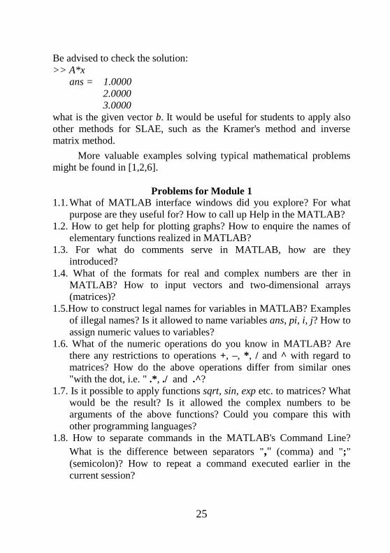
Be advised to check the solution:
>> A*x
ans = 1.0000
2.0000
3.0000
what is the given vector b. It would be useful for students to apply also
other methods for SLAE, such as the Kramer's method and inverse
matrix method.
More valuable examples solving typical mathematical problems
might be found in [1,2,6].
Problems for Module 1
1.1. What of MATLAB interface windows did you explore? For what
purpose are they useful for? How to call up Help in the MATLAB?
1.2. How to get help for plotting graphs? How to enquire the names of
elementary functions realized in MATLAB?
1.3. For what do comments serve in MATLAB, how are they
introduced?
1.4. What of the formats for real and complex numbers are ther in
MATLAB? How to input vectors and two-dimensional arrays
(matrices)?
1.5.How to construct legal names for variables in MATLAB? Examples
of illegal names? Is it allowed to name variables ans, pi, i, j? How to
assign numeric values to variables?
1.6. What of the numeric operations do you know in MATLAB? Are
there any restrictions to operations +, –, *, / and ^ with regard to
matrices? How do the above operations differ from similar ones
"with the dot, i.e. " .*, ./ and .^?
1.7. Is it possible to apply functions sqrt, sin, exp etc. to matrices? What
would be the result? Is it allowed the complex numbers to be
arguments of the above functions? Could you compare this with
other programming languages?
1.8. How to separate commands in the MATLAB's Command Line?
What is the difference between separators "," (comma) and ";"
(semicolon)? How to repeat a command executed earlier in the
current session?

26
Fig.1.6. Program MyClock
developed in MATLAB (see
program in Attachment A3)
1.9. What do the commands
length, size, inv, ' and diag? Do
you know other commands that
operate with matrices?
1.10. For a given vector, shift its
elements for one in counter
clockwise direction. (Hint:
remember construction (1.4)).
1.11. What mean the command
like x=-pi : pi/100 : 3*pi ? How is
it used for plotting graphs?
1.12. What of commands for
plotting graphs do you know?
What's the difference between the
commands plot, fplot, ezplot,
comet?
1.13. How may the commands legend, title, grid, xlabel, ylabel, axis,
insert "decorate" your graphs? How could you set or change color
of your plot curves?
1.14. For what do one use the command figure? If you need to plot
several graphics, how could you plot some of then in one window
but other curves in an other?
1.15. Plot the function given parametrically
ttx cos)3sin( , tty sin)3sin( , ],0[ t (1.9)
1.16.
How would it be possible to plot a discontinuous function like
in the example 2.2 or continuous piece-wise function in problems
2.12, 2.13?
1.17. How would you explain the difference between numeric, text and
symbolic data in MATLAB?
1.18. For a given matrix A find the mean of its elements.
1.19. How to find roots of a polynomial? How many are them? How to
find derivative and primitive of a given function? How to find a define integral?
1.20.
Develop a MATLAB program that displays current time like the
one shown in the Fig. 1.6. (Hint: use commands date and clock).

27
Module 2: Basics of MATLAB programming General module characteristics: Programming, i.e. making computer
programs is useful to automate calculations that you would repeat many times
otherwise, or to make calculations without manual intrusion. Commands
suggested by structural programming paradigm will be introduced, examples of
simple but motivating to further work programs will be given. Flow charts are
used to explain programs.
Micromodule 2.1. m-scripts and m-functions
To automate multiple repetitions of the same commands, one
writes programs. Actually, all the commands you learned previously
like fplot are the programs written by somebody. Now, let's become
programmer, too!
2.1.1. Scripts, the simplest programs
Assume, you need to systematically create triplets of functions,
say F1, F2 and F3, and then compare them by means of plotting their
graphs. These functions, each in the form of two arrays x={ x1, x2, … xn}
and F1={ F11, F12, … F1n}, may be created "by hands" like you did in
Module structure Micromodule 2.1. m-scripts and m-functions
2.1.1. Scripts, the simplest programs
2.1.2. MATLAB' Functions (m-functions)
2.1.3. Difference between Scripts and Functions
Micromodule 2.2. Structured programming
in MATLAB
2.2.1. Loop operator for … end,
2.2.2. logical operator if … else … end 2.2.3. logical arithmetic with and. or, not
Micromodule 2.3. More MATLAB' programs 2.3.1. Periodic Step-function
2.3.2. Least element of an array
2.3.3. Re-ordering of a vector
Micromodule 2.4. Supplementary problems 2.4.1. Dialogue programs
2.4.2. Debugging programs
Problems for Module 2

28
the Module 1.2. However, it would be a good idea to collect all the
commands required for plotting all three functions, i. e. their
visualization, and make the MATLAB to execute them by a single
command. Well, let us prepare a special file and save it under the name
visualize.m (with extension .m!). The text content of such a program
saved in a file is usually called its listing.
The following listing of the program visualize.m is suggested:
Listing 2.1 of the file "visualize.m":
1 % Example of a simple Script Program
2 % to visualize and compare graphics of three functions
3 % named F1, F2 and F3
4 % of argument x created previously in Workspace
5
6 % Copyright Ye. Gayev
7
8 figure; plot(x1,F1,'r', x2,F2,'b', x3,F3,'g')
9 title('Comparison of three Functions')
10 grid on;
11 xlabel('Independent argument X'); ylabel('Functions F of Х');
12 legend('F1', 'F2', 'F3')
13 % end of the script
Do the following to create this file practically: a) Press the icon
("New m-file") in the MATLAB; "m-File Editor" appears with an
empty window. b) Type above sentences line by line in this window. Do
not type numbers as the numbering will appear automatically. c) Having
typed all the text, press to save the file. Type the name visualize
instead of the name unnamed suggested. The file will be saved with the
extension .m in the subdirectory WORK. Before using it, let us analyze
its content.
Lines 1 to 6 start with the sign per cent % as well as the line 13.
This symbol denotes comments which the program does not account for.
The use of comments is explained below. Empty lines like 5 and 7 may
be used by programmer to better emphasize the structure of the program
and make it easily readable.
29
Section with MATLAB commands follow the comments.
Commands in the line 8 call new graphical window and plot all three
functions in one window with different colors, red, blue and green. The
command 9 prints the title in the window. Command 10 draws grids,
and the commands 11 label horizontal and vertical axes. Finally, the
command 12 provides legends which mean that the red curve
corresponds to F1, and so on. The line 13 is optional and serves for
denoting the end of the program.
Now, make few preparatory calculations and call the new
progam: >> % Create argument array
>> x1=-1 : .01 : 3; x2=x1; x3=x1;
>> % Create arrays with three functions
>> F1=x1; F2=F1 .*x1/2; F3=F2 .*x1/3;
>> % Finally, get result and analyze it!
>> visualize
A graph with three curves will appear. Problems 2.1 and 2.2 suggest
some exercises. The program visualize developed becomes a command
of MATLAB now that will be used several times in this book.
2.1.2. MATLAB' Functions (m-functions)
Another kind of MATLAB program is called m-functions. Let us
consider an example of a program that makes numerical differentiation.
Imagine, one has a number of function values y={y1, y2, y3, ….. , yN} that
correspond to arguments x={x1, x2, x3, ….. , xN}. One may interest in
getting knowledge how fast the function changes with the argument. In
the case of analytically given function y(x), its derivative y'(x) would
answer the question. We deal with a table function, so an approximate
formulae should be used9:
ii
iii
xx
yyp
1
1 , 1,...,1,0 Ni .
The program we would like to have should get arrays x and y and return
arrays y1 with derivatives and x1 with corresponding arguments (note
9 This formula uses "Differences Up". See any course of numerical mathematics
such [4] for alternative formulas.

30
that their lengths are less for 1, i.e. 1N ). The following program
MyDiff solves the problem.
Listing 2.210
of "MyDiff.m" 1 function [P,X1]=MyDiff(X,Y)
2 % This program returns Derivative of the function Y=Y(X)
3 % Copyright Ye.Gayev, July 2006
4
5 X1=X(1 : end-1); % Coordinates of the derivative P(x);
6 X2=X(2 : end); dX=X2-X1;
7 Y1=Y(1 : end-1); Y2=Y(2 : end); dY=Y2-Y1;
8 P=dY . / dX; % Formulae "Differences Up" is used
9 % End of differentiation
The program consists of 9 rows to be typed via the m-File Editor
and saved in a file with the name MyDiff.m. As before, lines 2 to 3 form
section with comments. Besides, comments serve for explanation and
providing additional information in lines 5 and 8. Note however that the
first line of any m-function should obligatory be the declaration function
along with definition that output variable OutVariable is linked with
input variable InputVariable through the function name FuncName. It is
declared by means of simple syntax
OutVariable =FuncName(InputVariables) .
In our case OutVariable is an array [P, X1] with variables P and X1, and
InputVariables are given arrays X and Y. The FuncName is MyDiff.
The command 6 creates an auxiliary array X2 with the data from X
but shifted for 1. Then, array dX is created in the line 6 with differences
between neighboring arguments. Similar, differences of function values
are stored in the array dY created on the line 7. Finally, 1N values of
the derivative is obtained by the command 8.
Note that presence of input and output arguments contrasts the m-
function with m-scripts where no arguments are used at all. Below is an
example of using the new program.
1. First, try asking help for the new program:
10
See the same program in the Attachment A1 in an advanced version that
analyzes "quality" of input and uses switch …end statement. See also program
MyDeriv, listing 2.10.

31
>> help MyDiff
This program returns Derivative of the function Y=Y(X)
Copyright Ye.Gayev, July 2006
It is to conclude: The Comment Section in each program serves for
getting help; it is worth to provide information in it about purpose of
this program, how to use it and other relevant information (copyrighted
person for example). Pay attention that it is very important to document
your program clear and completely! Another example see in Listing 2.4.
2. To work with the new program, let us get "experimental" data
by the following way (any function might be used instead of tsin ):
>> t=0 : 2*pi/10 : 4*pi ; y=sin(t) ;
(Note, the function data are rather rough because of a big increment
dt=10 ). Differentiate these data numerically:
>> % Examination of MyDiff program
>> [F1,x1]=MyDiff(t, y);
Now, get "experimental" data 100 times more precisely and differentiate
them again:
>> t=0 : 2*pi/1000 : 4*pi ; y=sin(t) ;
>> [F2, x2]=MyDiff(t, y);
It is worth to compare both results with original function )sin(ty in
the same Figure. First, one needs to rename t and y as x3 and F3, and
then visualize all three curves:
>> x3=t; F3=y;
>> visualize
Results have been shown in the Figure 2.1 and bring the following
conclusion: numeric function F1(x) is rather depart from the function
F2(x) which, in contrast, almost coincides with the exact derivative
ty cos of the given function. Students are advised to make
"computer experiments" by varying increment dt and even with other
functions, as suggested in Problems 2.1.3 to 2.1.6.
2.1.3. Difference between Scripts and Functions
It is important to account for several significant differences
between scripts and m-functions:

32
(i) Scripts do not have neither input parameter, nor output parameters in
contrast to m-functions that have them by definition.
(ii) Because of this, scripts may use any variables already defined in
MATLAB environment. In contrast, m-functions cannot "see" any
variables from the environment except those listed in InputVariables or
declared as global (see below). Their relation to the MATLAB
environment has graphically been illustrated in Fig. 2.2.
(iii) Similar to this, any variables created within scripts may later be
used in the environment (by a next script or m-function, for example). In
contrast, variables created within m-functions may be used within it but
are not "seen" from outside (unless they declared as global). It is
convenient: if you introduce any identity NewVar within function, you
do not need to check if it was defined somewhere before. From another
hand, when you leave m-function, the program immediately "forgets" all
variables created within it.
(iv) m-functions may contain internal (nested) m-functions that are
called subprograms or sub-functions (an example in Listing 2.7).
Similar to (iii), variable created in a nested function is not seen in the
external one.
Figure 2.1. Results of a "computer experiment" with numerical differentiation
by the program MyDiff: F3 is original, but F1 is its rough and F2 is more
precise derivatives.
F1
F2
F3

33
The "legal" way to supply variables to m-functions lies through
input variables. Input t,y and output variables F1,x1 in the above example
program MyDiff.m are called formal parameters of the program. They
are substituted by other real parameters when MyDiff is called.
This way may however be insufficient. Another one is declaration
of variables to be global, global NewVar1 NewVar2 . This should be
declared before the variable is created, both within the function and
outside it, or both in nested and external function. Be advised to check
visibility and values of such variables during debugging your complex
programs (see Micromodule 2.4.2)!
Micromodule 2.2. Structured programming in MATLAB
Computer programs given over might be called linear programs
as they are executed line-by-line in a top-down manner. Your programs
will be more "intellectual" if you apply logical operators in them. There
was a command GOTO in first algorithmic languages that could change
flow of program with respect to a logical condition. However, if
programs become sufficiently complex and hierarchical, they are
extremely difficult for reading and understanding them. It was so
suggested by N. Wirt and E.V. Daikstra (pronounce Дейкстра) not to
use the GOTO statement but use specially defined programming blocks,
control-flow statements, instead. Such kind of work was called the
structural programming11
. MATLAB's programming implements most
decisions of contemporary computer science. Flow charts may
significantly facilitate understanding of a complex program.
11
For details see http://en.wikipedia.org/wiki/Structured_programming.
MatLab' Environment with previously created data
x
a
b
Function x1, y Script x1, y
Fig. 2.2. Relations of scripts and functions with the whole MATLAB
environment: solid lines denote direct exchange of data while dotted ones
exchange by global variables.

34
2.2.1. Loop operator for … end
This composite operator allows repetition (loop) of several
statements a specified number of times. Its general syntax has the form:
for LoopVariable=Value1 : Increment : Value2
a statement or a command 1;
. . . . .
a statement or a command K;
end
This block of commands works in the following way illustrated by the
flow chart in the Fig. 2.3. First, the variable LoopVariable is set to the
initial value Value1. Condition if LoopVariable > Lalue2 is checked,
and statements and commands from 1 to K are executed because the
answer is false (No). Having reached the logical bracket end, the
program repeats execution of all the statements and commands from 1
to K again but with LoopVariable=Value1 + Increment. Next execution
uses LoopVariable=Value1 + 2*Increment, and so on until
LoopVariable becomes more than the value Value2. In this case, the
answer to the above question is true (Yes), and the program block ends
its work.
Comments: 1. The Increment may not be obviously positive; in
the case of negative Increment, the value of LoopVariable each time
reduces. 2. The loop described may be prematurely terminated by the
statement break, see Help break. 3. Each of statements may use the
operator for …end again. Such new loop would be called the nested
loop. Let's learn few examples.
Example 2.1. Rotation of a stick on your PC screen.
You easily can, of course, plot a static stick with coordinates
)sin,(cos tt and )sin,cos( tt on your PC screen for any given
value t . For example:
>> t=pi/4 ;
>> x1=cos(t) ; y1=sin(t) ;
>> x2=-x1; y2=-y1;
>> plot([x1 x2], [y1 y2], 'b', [0], [0], 'or')
The straight line you see on the screen is symmetrical against centre
)0,0( that is emphasized by red circle. The program helicopter uses the
for …end operator to rotate this stick on your screen:

35
Listing 2.3 of the script "helicopter.m" %Script HELICOPTER
% produces a stock that revolves N times
% in counter-clockwise direction.
% Copyright Ye.Gayev, May 22, 2005
Dt=.1*pi; N=10;
for t=0 : Dt : 2*N*pi
x1=cos(t) ; y1=sin(t) ;
x2= -x1; y2= -y1;
Pl=plot([x1, x2], [y1, y2], 'r') ;
set(Pl, 'linewidth',4 ) %See Help or Module 4 for explanation of set !
axis([-1.1 1.1 -1.1 1.1]) % Why do we use this?
hold on; plot([0], [0],'o'); hold off;
pause(.1) % See Help for pause
end
% End of helicopter
Comments: 1. Mistakes in program may lead to getting caught in an
endless loop. Use keys <Ctrl + C> to break loop and stop the program.
2. More sophisticated operators while … end and switch … end could
also be very useful in practice; see Help for them. Few more examples
of for-loop have been given in listings 2.7, 2.9 and A1 (MyDiff).
2.2.2. Logical operator if … else … end
This command makes your programs more "clever". Its simplest
syntax looks as
if LogicalExpression
Statements1
else
Statements2
end

36
This command block is self evident, so we may explain it by an
example.
Example 2.2. Make MATLAB to understand the following
mathematical piece-wise Step-function (that is associated with famous
Heaviside and Dirac functions)
Fig. 2.3. Flow chart of the for … end statement
true
false

37
It means, MATLAB should calculate value of the Step function, i.e. +1
or -1, for each (at least single) argument x and plot its graphics shown
on the right hand-side. The program Step01 solves this problem.
Listing 2.4 of "Step01.m" function y=step01(x)
% Program-function to plot piece-wise function
% / +1, if x > 0
% y=|
% \ -1, if x <= 0
% Example of use: ezplot('step01(x)', [-3 3]).
% Copyright Ye. Gayev, Nov. 2005
if x<0 % Note: this is a Logical Expression !
y=1; % Here is Statement1
else
y=-1; % Here is Statement2
end
% End of Step01
Let us explain now how this program works:
1. If one asks MATLAB for a help,
>> help Step01
the answer is
Program-function to plot piece-wise function
/ +1, if x > 0
y=|
\ -1, if x <= 0
Example of use: ezplot('step01(x)', [-3 3]).
So, the program uses the information provided in the Comment Section
to remind to user how this function looks like and how to use it. We
may follow to the last advice.
0,1
0,1
)(
xif
xif
xy

38
2. Try to calculate this function for several argument values, for
instance:
>> y1=step01(2), y2=step01(-2)
y1 = 1
y2 = -1
So the program calculates correct.
3. Now, plot the graph of the Step-function in the way recommended:
>> fplot('step01(x)', [-2 2 -1.2 1.2])
Graphics similar to the above picture is to be displayed. Congratulation:
MATLAB knows now the new mathematical function you've created!
Pay attention however that the function works wrongly for array
arguments. Try for example and get a strange answer:
>> x=[-2 -1 1 2]; y=step01(x)
y = 1
Our next aim will so be to teach our program to understand arrays. For
this, consider problems 2.11 – 2.13 and learn Micromodule 2.2.3. At the
moment, however, consider a new useful example.
Example 2.3. Develop a program welcome that will greet you
with regard to the day or night time moment and remind you to go
sleeping when it is too late (take control moments 6 a.m. and 1, 6 p.m.
and 0 a.m.). The program should be of course of the script type:
Listing 2.5 of "welcome.m" % Script WELCOME
% greets the User depended on the part of Day or Night
% divided into 6 hours, 13, 18, 24 and [0, 6] hours
% Copyright of Ye. Gayev, Dec. 2005
T=clock; %Returns the array [Year, Month, Day, Hours, Minutes, Seconds]
if (T(4)>5) & (T(4)<=12)
disp(' ') % to get an empty string on the screen
disp('Good morning!')
elseif (T(4)>12) & (T(4)<= 17)
disp(' ')
disp('Good afternoon!')
else

39
if (T(4)<= 23)
disp(' ')
disp('Good night!')
else
disp(' ')
disp('Good night. But I wish you slept this time!')
end
end
Explanation. First, the program uses two MATLAB commands
unknown to you, clock and disp. Ask Help about them or/and try them
from the Command Line. You will be answered with concern to clock
that it returns a numeric vector with six elements that corresponds to
date and time moment in the format noticed in the comment of the 7th
line. We need to work with the only 4th element T(4).
Secondly, the IF-operator we study is applied in its general form
here,
if LogicalExpression1
Statements1
elseif LogicalExpression2
Statements2
else
Statements3
end
The latter works in the following way. Having reached the if-operator,
computer checks the LogicalExpression1. If it has the value true12
,
12
See next section 2.2.3.
P
S1
S2
Fig. 2.4. Flow chart explaining logical operator if … else.
Yes
No
true
false
Fig. 2.4. Flow chart explaining logical operator if P … else S2.

40
several Statements1 are executed after which the program leaves the if
… end block at all. However, if the LogicalExpression1 is false, the
portion of if-block between elseif and end becomes working. Again,
LogicalExpression2 is checked. If it is true, Statements2 are executed
and the program goes outside the end. However, if LogicalExpression2
equals false, the Statements2 are skipped and Statements3 are executed
after which the program comes to the line next after end. See also
illustration in the Fig. 2.4.
First two groups of Statements include two commands. It is
important to note that Statements3 contain one operator that is a nested
operator if…else…end. The latter works as explained over. Another
point to draw attention is the manner of writing all the above programs:
they look graphically out like steps. Students are advised to always write
your programs in such a way to emphasise blocks and other structural
elements of the program. MATLAB' m-file Editor makes this
automatically what evidences a "good taste" of this programmer!
2.2.3. Logical arithmetic with and, or, not
In the listing 2.5, we met complex logical expressions like
(T(4)>5) & (T(4)<=12)
that consists of two elementary expressions T(4)>5 ("Element T(4) is
more than 5") and T(4)<=12 ("Element T(4) is less or equal than 12").
What is the logical expression?
It is a sentence that may be estimated in terms of true or false, i.e.
may have values of 1 or 0 only, and depends on the variable argument.
(Sentence itself does not depend on any argument; for instance, sentence
"The sun rises in the West" is always false). Say, in 3 o'clock the
expression T(4)>5 gets the value 0 (false) while in 7 a.m. its value is 1
(true). Elementary logical expressions may include relation signs as
= = (equal13
) < (less) > (more)
<= (less or equal) >= (more or equal) ~= (not equal).
Like in every-day-life, we can formulate complex expressions
from elementary ones. Binary logical operations
& (AND) and | (OR)
and unary logical operation
13
Note that one assignment sign = cannot be used for relations!

41
~ (NOT)
are used for doing this. Logical value of complex expressions may often
be estimated by intuition; for example, the expression
(T(4)>5) | (T(4)<=12)
equals true both in 3 and in 7 o'clock. However, computers require
rigorous formal rules. The latter, known as logical arithmetic, have been
given in tables below.
A&B A | B
A=true A=false A=true A=false
B=true 1 0 1 1
B=false 0 0 1 0
~ A
A=true false
A=false true
Most of algorithmic languages do not mix logical and arithmetic
operations. In contrast, MATLAB allows mixing of both: a number may
multiply logical expression A, and the result is either the same number if
A=1 (true),or zero if A=0 (false). This MATLAB' feature lead to
simplification of many programs.
Recall the programs Step01 for plotting discontinues function.
Here is its modification.
Example 2.2,A: Step-function programmed with MATLAB'
logical feature.
Listing 2.6 of "step02.m" function y=step02(x)
% Program-function to plot piece-wise function
% using features of the MATLAB Logic
% / +1, if x > 0
% y=|
% \ -1, if x <= 0
%
% Example of use: ezplot('step01(x)', [-3 3]).
% The command plot may be used as well.
% Copyright Ye. Gayev, Nov. 2005
y1=(x<0);

42
y2=(x>=0);
y=-y1+y2;
% End of "step02.m"
It is easy to check that all the easy-to-use plotting programs do work
with this command, for instance:
>> fplot( 'step02(x)' , [-3 3 -1.1 1.1])
Check also that the program is applicable to array data:
>> y=step02([-2 -1 0 1 2])
y = -1 -1 1 1 1
It is no wonder so that the command plot does work too:
>> x=-4 : 8 / 1000 : 4 ; y=step02(x) ;
>> plot( x , y), axis([-4 4 -1.1 1.1])
We have thus taught MATLAB to understand array arguments what is
in compliance with the MATLAB's "matrix philosophy". Compare this
function step02 with another one step03 suggested by the problem 2.11.
Micromodule 2.3. More MATLAB' programs
Three more programs placed below have to enhance your
programming skills and are thus useful for further applications in other
disciplines.
2.3.1. Periodic Step-function
An important role in mathematics, physics and informatics plays
periodical modification of the Step-function in Example 2.2, with period
2 for example:
]2,2(,1
]2,2(,1
)(
kkxif
kkxif
xy
,...2,1,0k
Its graphics recalls the function xsin but is discontinues. How to define
this function in MATLAB, how to plot its graphics? Program Step_pi
has been suggested here.
The following algorithm is suggested for determining )(xy for
arbitrary x . First of all, check if ],[ x . If Yes, any previously
developed function Step01, Step02 or Step03 may be used to assign to

43
y the value either 1 or 1 . We would suggest this to be a nested
subfunction step, see Listing 2.7.
If the answer is No, let us shift along axis Ox periodically for 2
to the right (or to the left) until x will be captured into the interval
]2,2[ kk of the length 2 where ,...3,2,1 k (or
,...3,2,1 k ). It is not clear in advance how many steps are to be
done (and thus the while –loop is to be used), but it is evident that the
process will be finite. When this happens, the same function step may
be used. Such shifting is equivalent to subtractions 2xx if
0x and to additions 2xx if 0x . This algorithm is
schematized in the flow chart in Fig. 2.5. Listing 2.7 realizes the
algorithm for MATLAB.
Listing 2.7 of step_pi.m function F=step_pi(x)
% Periodic Step Function,
% i.e. 2*pi-periodical continuation of the Step Function
% / =-1; if x \in [-pi, 0]
% F(x)=|
% \ = 1, if x \in (0, pi]
% Copyright Gayev Ye.A., January 2006
L=length(x); % See HELP for this function
for i=1 : L % Begin of loop № 1 on vector elements
xx=x(i);
if (xx >= -pi) & (xx < pi) % If xx \in [-pi, pi]
% disp('x within [-pi, pi]');
F(i)=step(x(i));
elseif xx <= 0 % If xx out of [-pi, pi] and negative
% disp(' X < 0 ' );
nT=0;
while ~ ((xx >= -pi) & (xx < pi))
%Begin of loop № 2 until xx \in [-pi, pi]
nT=nT+1; xx=xx+2*pi ;
end

44
% End of loop № 2
F(i)=step(xx);
else % If xx out of [-pi, pi] and positive
% disp(' X > 0 ' );
nT=0;
while ~((xx >= -pi) &(xx < pi ))
%Begin of loop № 3 until xx \in [-pi, pi]
nT=nT+1; xx=xx-2*pi;
end
% End of loop № 3
F(i)=step(xx);
end % Закінчення перевірки положення xx відносно [-pi, pi]
end % End of loop № 1
Fig. 2.5. Flow chart of periodical function Step_pi
true true
true
true
true
false
false
false
false
false

45
% End of the program step_pi
%-------------------------------------------------------------
% Example of (nested) SubFunction
%-------------------------------------------------------------
function F=step(x)
% Step Function equals -1 if x \in [-pi, 0] but = 1, if x \in (0, pi]
if x<=0
% disp( ' SubProgram X<0' )
F=-1;
else
% disp( ' SubProgram X>0' )
F=1;
end % End of SubFunction
It may be checked that the program step_pi works for array argument.
Comments to program. 1. Program length(x) determines the
number of elements of x. 2. Command disp(' Text ') displays the text
Text on computer screen. Such commands are useful during debugging
of programs and checking if it follows the logic you incorporated. They
may be either deleted or commented by % after tuning the program.
2.3.2. Least element of an array
An one-dimensional array X is given consisted of numeric
numbers. Develop a program MyMin that returns the least element of
them along with its position in the array.
Algorithm of the program is clear from MATLAB program in the
listing below. It is assumed initially that Xmin is the first element of X
and its number is Imin=1.
Listing 2.8 of MyMin.m function [Xmin, Imin]=MyMin(X)
%Program for determination of smallest element of the vector X
% for teaching purposes
L=length(X);
Xmin=X(1); Imin=1;
for i=2:L
if X(i) < Xmin
Xmin=X(i); Imin=i;
end
end

46
Similar to this program, a program MyMax may be developed that
looks for greatest element of input array and its position. It is assumed
below, in the next section, that this program exists. In fact, such
programs min and max have already been included as built-in functions
of MATLAB. It would be of interest to compare whose function is
better, see Micromodule 3.4.
2.3.3. Re-ordering of a vector
Reordering elements of vectors is a key problem of computer
science: for given vector X, return vector Y with the same elements
ordered in ascending or descending order. The program MyOrder below
analyzes one of arguments to be either Increase or Decrease, and warns
user to correct the task otherwise. The following algorithm is used for
the case Decrease for example. The problem is solved by L=length(X)
steps. Each time i=1, 2, …, L an auxiliary array X1 with elements from
X is checked, its greatest element by MyMax is found, placed to the i-th
place of another auxiliary array y and new array X1 is created with those
element absent. Try to draw flow chart of the algorithm yourselves
(problem 2.15.). The latter is realized in the following program.
Listing 2.9 of MyOrder.m
function Y=MyOrder(X, Order)
% Return vector Y with the elements of the argument vector X
% / increasing elements if 'Order' is 'Increase'
% but ordered accordingly to |
% \ decreasing elements if 'Order' is 'Decrease'
%
% Example: Y=MyOrder([1 2 3], 'Decrease') returns Y=[3 2 1].
% Uses MyMax and MyMin already developed
% Copyright Ye.Gayev, Dec. 2005
L=length(X); X1=X;
switch Order
case {'Increase', 'increase'} % Rearrange X in Increasing Order
for i=1 : L
[Y1,I]= MyMin (X1);
y(i)=Y1; X1=[X1(1 : I-1), X1(I+1 : end)];
end
Y=y;

47
case {'Decrease', 'decrease'} % Rearrange X in Decreasing Order
for i=1 : L
[Y1, I]=MyMax(X1);
y(i)=Y1; X1=[X1(1 : I-1), X1(I+1 : end)];
end
Y=y;
otherwise
disp(' ')
disp('It should be either "Increase" or "Decrease" in the second entry.')
disp('Check your problem and try again, please!')
disp(' ')
end
% End of the Program
The program in the above example works irrelevantly on letter
case, either 'Decrease' or 'decrease'. Such programs that analyze input
not to include errors and warn user if so, create am impression of being
intellectual. The program works with only row-vectors, then. It could
easily be generalized however for matrices, as in below program:
Listing 2.9A of My1Order.m
function Y=My1Order(X, Order)
% Function returns matrix Y
%with the same dimensions as matrix X
%but elements of each row re-ordered as stated by Order.
% "MyOrder.m" is used as sub-program.
% Copyright Ye. Gayev. October 2006.
[N,M]=size(X); %N=number of rows in X
for i=1:N
Y(i, : )=MyOrder(X(i, : ),Order);
end
Algorithm realized in the programs is one among several known
algorithms of sorting, see [8,9] and problem 2.16. Because of
importance of such algorithms in computer science, similar function sort
was developed in MATLAB. A question will be addressed in
Micromodule 3.4 which of algorithms "is better".
Micromodule 2.4. Supplementary problems
2.4.1. Dialogue programs

48
It is expected that computers will understand oral commands and
communicate with us by voice in the future. Making computers so
intellectual will also be up to you when you become specialist. Now, we
shall make a first step and teach computer to communicate in a form of
dialogue from the Command Line. Next step, communication with
computer via Graphical User Interface, will be done in the Module 4.
Three ready MATLAB commands are sufficient to us here. The
command disp(x) displays value of variable x, i.e. matrix in general
case, without printing the name of variable; the command disp(' Text ')
displays the text provided in inverted commas. The command
X=input(' PromptText ')
prints the text PromptText on the PC screen, waits for any input from
the Command Line and assigns the latter to the variable X. Finally, the
command pause (in its simplest syntax) stops the program until any key
is touched.
Example 2.4.1. Develop a program MyDeriv that greets you,
introduces itself and asks for which mathematical function would you
like to get derivative function, and finally compares graphics of both
origin and derivative. The following program realizes one of possible
solutions.
Listing 2.10 of MyDeriv.m % Script of a Dialogue Program
% that plots function provided by User
% and compares it with its derivative
% Copyright Ye.Gayev, June 2005
welcome;
disp(' '); % to make space between lines
disp(' Here is Command Line Dialogue Program '); %Commands to dialogue
disp(' for analytical calculation of derivative ');
disp(' of a function you will be asked for.');
syms Fname x % List of variables to assign symbolic values
disp(' ');
disp('So, please input a Function of x which Derivative')
disp(' you would like to compare with. ')

49
Fname=input(' '); % Introducing function to differentiate
Deriv=diff( Fname );
disp(' You introduced function y=');
pretty( Fname )
disp(' Its derivative is y=');
pretty( Deriv )
disp(' ');
disp('Press any key and compare them in two graphics!')
pause
figure; ezplot(Fname); title( 'Plot of your function')
figure; ezplot( Deriv ); title(' Plot of your derivative')
disp(' ');
disp('Thanks for using this program!')
% End of MyDeriv
Please analyze yourself how this program works bearing also in
mind comments in it. In developing programs of dialogue types, you are
advised to do all your best for making your program polite and clear, i.e.
sufficiently documented, for users.
2.4.2. Debugging programs There is a saying among experienced programmers "No program
may appears at first without errors". Errors may be occasional mistypes
or even logical errors in programming. That is why you are
recommended to draw flow charts for each complex program. Anyway,
debugging is required to check each new program in all possible
situations.
If your program contains mistypes or syntax errors, MATLAB
produces a message colored red like
"??? Undefined function or variable '. . .'", or
"??? Error: File: C:\MATLAB6p5\work\MyDeriv.m
Line: 22 Column: 19 ")" expected, ";" found".
Find error in program by m-file Editor and correct it.
The most insidious and hidden are logical errors, however. To
prevent them you are advised to split each complex program to blocks
or sub-programs and check them. Being sure in parts, check your
program as a whole. You shall often come back to program text in m-
file Editor. It may be useful to find critical points of the program and

50
place control prints like disp('I am at point A') there to check if the
program passes them properly. Having tuned the program, delete those
checking points or, rather, comment them by %.
In fact, this technique realized in the m-file Editor so that you may
do the same through menus Debugging and Stop Points. Try this! This
service found further development in versions 7.1 till 7.3 of the
MATLAB.
It may be thought that MATLAB is an interpreter rather than
compiler what means that it cannot produce autonomous executive files.
In fact, it was true for its versions less than v.5. In later versions, a
possibility was developed to compile exe-files and thus accelerate
execution of MATLAB programs unless the latter does not include
complex structures like graphic windows. It is declared for recent
versions v.7.x that all such restrictions have already been eliminated. So,
welcome for developing applications of your own!
Problems for Module 2.
2.1. Visualize three consequent functions given by recurrence formula
)!2()(
2
n
xxf
n
n for ,...2,1,0n
2.2. Visualize three consequent functions given by recurrence formula
)!12()(
12
n
xxf
n
n for ,...2,1n
2.3. Imagine a process governed by a law tey . You sample however
separate values of this function for certain time instances. Investigate
how time increment affects accuracy of numerical differentiation by
MyDiff.
2.4. The same question with regard to function xy .
2.5. Try to develop a program for numerical integration using definition
of define integral from your mathematics course. How increment
x influences accuracy of the result?
2.6.
Investigate problems 2.3 to 2.5 for a case that "experimental
data" contain occasional errors modeled by command14
sigma
14
Look in Micromodule 3.3 or ask Help for this command.

51
*randn(1,1) that generate random numbers distributed normally with
dispersion sigma=0.1. Analyze if differentiation and integration are
sensitive to such errors.
2.7. In the program helicopter make the stick to rotate in clockwise
direction.
2.8. Develop the program that revolves "the rose" (1.9) of the problem
1.15 in clockwise or anticlockwise direction. Figure 4.6. looks
similar to what you should get.
2.9. Develop a program that plots a pulsating ellipses.
2.10.
Develop dialogue program that asks for N and revolves polygon
with N vertices in either clockwise or anticlockwise direction. Try
using fill command to fill in polygon with a color of choice.
2.11. Modify the program of the Example 2.2 to make the Step01 to
understand vector argument by means of loop operator for...end; use
plot command. Name the new function Step03.
2.12. Develop program for calculating and plotting graphs of the
following 'Saw-like' mathematical function
]1,0(,1
]0,1[,1)(
xifx
xifxxf
.
2.13. Develop program that calculates values and plots graphics of the
following piece-wise "trapezoidal" mathematical function that
consists of 3 branches:
]2,[),2(2
],[,2
],0[,
1
2
24
xifx
xif
xifx
y .
(Hints for problems 2.12 – 2.13: students are advised to develop several
programs with gradually increasing difficulty like it was for functions
step01, step02, step02 and step_pi, i.e. (i) program that understands
single arguments but can ezplot and fplot for the domain given; (ii) program
that understands vector arguments and may be used for plot command; and
(iii) that for function periodically continued to the whole domain
x ).
2.14. Develop program MyMax mentioned in section 2.3.2 that looks for
greatest element in arrays; draw flow chart for it. Pay attention to
documenting your programs by comments % to make them clear to
other person, or even for you a year later.

52
2.15. Draw flow chart of the program MyOrder developed in section
2.3.3. Generalize the program to make it to "understand" two-
dimensional input argument (matrices).
2.16.
Learn "bubble" method of sorting [7-9] and realize it in a
MATLAB program. Analyze, what of such algorithms already
known to you is better.
2.17. Analogically to MyDeriv, develop dialogue program for
comparing functions and their primitive (define integral) to be found
"analytically", see Micromodule 1.3.2.
2.18. You certainly may solve the problem 1.20 now. Try this!
2.19.
A number of exciting and useful programs may be developed by
reader now. Some our students made their term papers named
"MATLAB Guide to Analytical Geometry", or "Test your
Knowledge of Functions by MATLAB", etc. You are advised to
follow them!

53
Module 3: MATLAB for learning and investigation General module characteristics: Despite you have spent rather few time
for mastering MATLAB yet, you have already been able to get a significant
advantage in learning your university disciplines, especially such difficult ones
as mathematics and physics. It must be confessed that mathematics is often
taught somewhat scholastic. However, you can now check many of its
statements "experimentally". Really, many scientific facts were found by
similar "numeric experiments". Few examples below may help you in doing
this and encourage you for further investigations on your own.
Module structure Micromodule 3.1. The awful "ε – δ language"!
Micromodule 3.2. Taylor, Fourier… Who else?
Micromodule 3.3. Discovering empirical formulas
Micromodule 3.4. Efficiency of programs
Micromodule 3.5. Your further discoveries with MATLAB
Problems for Module 3
Micromodule 3.1. The awful "ε – δ language"!
It is our experience in teaching that students conceive definition of
the limit with difficulty; introduction of ε and δ in this definition leaves
unclear to them. Well, let us try to investigate "where function or
sequence tends to" by means of self-evident literal calculations by
MATLAB.
1. Consider the famous "Second Famous Limit". It states that the
numeric sequence nnns 11 tends to a certain border value when
integer number n grows unrestrictedly. The program limit1 presented in
its listing is convenient to plot the sequence ns step by step in a form of
dialogue. Strings in the listing have been numbered for convenience in
explanations.
Listing 3.1 of limit1.m 1 %This script calculates and plots numeric sequence
2 % s(n)=(1+1/n)^n known as the First Famous Limit.
3 % After each N calculations the program stops and asks
4 % if it should stop or go on in calculations. By default, N=10,
5 disp('This program investigates The Second Famous Limit');
6 disp('=========================')

54
7 N=10; n1=0;
8 Answer=1;
9 while Answer > 0
10 for k=1 : N
11 n(n1+k)=n1+k; s(n1+k)=(1 +1/(n1+k))^(n1+k);
12 end
13 n1=n1+N;
14 plot(n , s ,'-', n , s,'or');
15 title('Investigation if s_n=(1+1/n)^n has a limit.')
16 xlabel('Number n'); ylabel('s_n');
17 text(5, 2.1,'\bf Use the Command Line for further commands...')
18 if n1==N
19 str0='First ';
20 else
21 str0='Next ';
22 end
23
24 disp([str0, num2str(N),' points have been added to the plot.'])
25 disp('Analyze results and deceide if I am to go on.')
26 disp ('Imput any positive number to go on,')
27 Answer=input('or a NEGATIVE NUMBER to complete!');
28 disp('-------------------------');
29 if Answer < 0
30 disp('--');
31 disp('I"ve finished the work on your request. Thanks!')
32 disp('====================================');
33 end
34 end
35 disp('Enjoy your results and draw conclusions!')
36 clear n
Comment to program. The program works in the following way.
Being run, it explains what it serves to ('This program investigates The
Second Famous Limit'). Having plotted fist graph for Nn 1 for the
specified 10N , the program stops and asks user if it should finish or
go on in calculations. Input of any positive number continues
calculations and plotting for next N steps. To finish, input any negative
number, say -1. This logic has been realized by the while … end loop, 9
– 34. Each next N calculations are added by the for-loop, 10 – 12.

55
"Logical behaviour" of text 24 is managed by the if-block 18 – 22.
Transformation of numbers to characters by procedure num2str(N) and
concatenation of strings was used here, see [1]. In concern of proper
writing sub- and superscripts by the line 15, ask MATLAB for available
TeX characters what is useful also for making text bold (command \bf in
line 17) and writing Greek characters.
Comment to mathematics. Graphical results of calculations
have been shown in Figure 3.1. It is shown for the range 301 n but
may be extended to any length. It may be suggested (and proved by
further calculation) that ns never exceeds certain values, say 8.2ns .
Fig. 3.1. Plotting sequence sn of the Second Famous Limit by the program
limit1. Analysis determines that (i) sn tends to a certain limit (find it
yourself!) and (ii) sequence elements grow monotonically.

56
Note also that ns grows monotonically, the fact you used in formal
proof.
Numeric value that the ns can never exceed may be defined more
precisely. Do this yourself! With MATLAB, you unlikely require two
hundred years as mathematicians of 16th and 17th centuries did.
However, they discovered that this number is transcendental and gave a
special name e that since has widely been used in logarithms and in
mathematics at all.
Here was the first example how programming converts boring
school tasks into interesting research! MATLAB's command limit may
also be useful in learning function.
2. Let us consider another problem associated with limits and
sequences. The latter is called recurrent sequence if its nth element may
be calculated by means of a previous one, of (n-1)th, through a recurrent
formulae. Consider quadratic formulas Css nn
2
1 where 0s and C
are allowed to be complex numbers. Having chosen complex initial
element 0s and complex constant C , get complex elements 1s , 2s ,
…, ns and look where they tend while n . Because they are
complex, each element corresponds to a point on the plane xOy with
coordinates )Re( nn sx and )Im( nn sy 15.
Does such sequence have always its limit? It depends! Take
different complex 0s and C , and try. The path the sequence ns
converges or diverges16 may be very different but often forms a
strange picture. Two of them obtained for .01i0.150s are
shown in Fig. 3.2. The left one that resembles a spiral galaxy
converges counter-clockwise was obtained with .6i- -.05C . In
the right picture obtained with .35i.36C the current point ns
jumps between five "spots" that behave as a clockwise diverging
15
Real and imaginary parts of complex number that correspond to MATLAB
functions real(s) and imag(s). 16
These terms mean 'tends to a limit position' and 'does not tend'
correspondingly.

57
galaxies on the screen. In the case 0.5651i -0.1238C
"galaxies" tend to complex point 3897i0.225- along linear
trajectories. You are advised to get more funny pictures! It is
worth to examine constants i..C 1080 , i.. 120690 , i.. 1070 ,
i.. 120690 and i.. 5868039050 with 00 s . Despite they are so
strange, the area belongs to very recent science of fractals [7]
where one could get more information.
Micromodule 3.2. Taylor, Fourier… Who else?
These are famous names that mentioned in the title. Theorems of
both are studied in Higher Mathematics course. The theorems sound
similar.
Taylor's theorem: for almost any17
function )(xf , a polynomial
n
nn xaxaxaaxT 2
210)( may be found that approximates
it; the more is n the close is proximity of both.
Fourier theorem: almost any periodic function )(xf may be
approached by a trigonometric polynomial
17
Precise sense of important terms "almost any" and "approximate" (or
"approach") look in handbooks.
Fig. 3.2. Two plots of complex quadratic sequence that resemble one
converging (left) and five diverging (right) spiral "galaxies".

58
)2cos2(sin)cossin()( 22110 xbxaxbxaaxTn
)cos(sin nxbnxa nn ;
proximity becomes "better" for bigger n .
Strict proof of the theorems is given in textbooks. MATLAB is
useful to examine the theorems by example.
Example 3.1. Validate by means of plotting that the below
Fourier polynomial
converges to the Step-function
),0( ,1
)0,( ,1)(
x
xtf .
Solution of the problem gives dialogue program whose listing is
given below.
Listing 3.2 of Script "Fourier1.m" % This Command Line Dialogue Script
% plots periodical Step Function over area a < x < b provided by user
% and graphically compares it with two approaching Fourier polynomials
% whose orders n1 and n2 are also requested from user.
% Copyright Ye.Gayev, February 2006.
welcome; % to greet user
disp('================================')
disp('This program plots periodical Step Function over area a < x < b')
disp('(you will be asked about values a and b)')
disp('and compares it with two approaching Fourier polynomials of the form')
disp('Fn(x)=4*(sin(x)+sin(3x)/3+sin(5x)/5+ ... +sin((2n-1)x)/(2n-1))/pi.')
disp('You will be asked about orders n1 and n2 of the two polynomials.')
disp('--------------------------------')
disp('Press any key to start.'); pause
% Dialogue start
disp('Please enter in brackets a and b,')
A=input('interval endpoints, to plot the functions: ');
disp('--------------------------------')
disp('Here are endpoints of the interval to plot:'); A
disp('Please provide two integers in brackets, orders of the polynomials: ')
N=input(' orders of the polynomials: ');
disp('================================')
12
)12sin(...
5
5sin
3
3sin
1
sin4)(
n
xnxxxxFn

59
disp('Thanks! Now, analyze results in Figure.')
% Creating fist polynomial in symbolic form
F1=' ' ;
for i=1:N(1)
Coefficient=num2str(2*i-1);
Summand=['4*sin((', Coefficient, ')*x)/pi'];
F1=[F1, '+', Summand];
end
% Creating second polynomial in symbolic form
F2=' ';
for i=1:N(2)
Coefficient=num2str(2*i-1);
Summand=['4*sin((', Coefficient, ')*x)/pi'];
F2=[F2, '+', Summand];
end
ezplot(F1,[A(1), A(2)]);
hold on; fplot(F2, [A(1), A(2)], 'g');
title('{\bf Step(x)} (red) {\bf compared with F_1(x)} (blue)
{\bf and F_2(x)} (green)')
Comment to program. The dialogue managed by the program
seems to be clear both from programming and user aspects. It begins
with the command welcome that greets user in the way already
described. Both trigonometric polynomials to plot are created in
symbolic form by addition terms step-by-step. Variable Summand
represents regular term in each loop, so that F1 and F2 get the form of
required polynomial at the end. Command fplot was chosen for plotting
second polynomial, as it may control (in contrast to ezplot) colour of
lines. Using TeX commands gives the better featured title.
Comment to mathematics. Try calculations over different
domains [a, b] and, what is more important, for polynomials of different
orders and analyze results. Figure 3.3 presents graphical output for
domain ]2,[ , i.e. one and half period of the Step-function, where
the Step-function is compared with polynomials )(3 xF and )(7 xF .
Similar, polynomials of elder order may be compared with it. In fact, it
may be concluded that trigonometric polynomials wave over both steps

60
of the function. The number of waves corresponds to polynomial order
n . It may be thought that none of them "approximate" the function,
even if n . Higher mathematics introduces however another idea
of "proximity of two functions" in terms of integrals (areas). And this
proximity between the Step-function and )(xFn tends to zero while
n , what turned to be very useful in mathematics, signal
processing and informatics at all.
Investigation of the Taylor' theorem is advised to carry out
yourselves. MATLAB's command taylor is useful in finding polynomial
expansions "analytically".
Micromodule 3.3. Discovering empirical formulas
This is a common problem in physics, sociology, economical
science etc. to look for analytical formulas for representing experimental
(or obtained by other means) data. MATLAB suggests a wonderful tool
for solving this problem called "curve fitting".
Fig. 3.3. Graphical output of program Furier1 allows investigation Fourier
polynomials that approximate Step function. Result for 31 n and
72 n (see Problem 3.4, then).

61
Let an observation was carried out in time moments t=1:.5:6.
Imagine, we know (but nobody else!) the law baty with
coefficients, say 2a , 3,0 and 1b , the process )(ty is
governed by. If one would sample values of y in given moments,
results were certainly different from those theoretical values because of
measurement errors. How to get "experimental" data to learn an
example? MATLAB allows a "numerical experiment". The command
rand(1,n) can generate vector 1*n of random numbers uniformly
distributed between 0 and 1. However, use the command
Eps*randn(1,n) that generates normally distributed random numbers
with dispersion Eps as it always happens in any measurement. So, the
following commands produce theoretically "exact values of y" Yexact
along with their "experimental" representatives Yexp with "stochastic
errors":
>> t=1:.5:5; a=2; Alpha=.3; b=1; Yexact=a*t.^Alpha+b;
>> Eps=.1; L=length(t); Yexp=Yexact+Eps*randn(1,L);
Fig. 3.4. Figure Window (middle) with exact "experimental" data and their
linear (B), cubic (C) fits and that of 8th order (A) found via Fitting Interface
(left). Right: two possible straight lines going exactly through two "experimental"
points.

62
>> plot(t,Yexp,'o', t,Yexact,'--')
The last command results evidently in plotting dashed "theoretical
curve" and "experimental" circles18
, Fig. 3.4; the more is Eps, the more
the circles are scattered around the curve. The number of "experimental
circles" L has been determined by length(t). The curve fitting problem
sounds: find equation to represent experimental data. Once we have it,
we could interpolate experimental data (i.e. get )(ty between measured
points), or even extrapolate them (i.e. estimate )(ty in the past, or
forecast )(ty for future). Note that problem formulation is not
addressed to finding precise law of the process what should be looked
for in particular scientific discipline; the problem lies in selection among
specified set of functions such as linear 21 ptpy , polynomial
1
1
21 ...)(
nn
nn
n ptptptptP , exponential or other
functions [3,4].
To start our analysis, choose ToolsBasic Fitting in the Figure
menu. The Basic Fitting Interface that appears is shown in the Fig. 3.4,
left on the Figure window. First, choose data1 in the window 1 as the
data2 relate to "exact" values of the function and will be used for
comparison only. Secondly, we should "experiment" with type of the
approximation: functions from linear to 10th grade have been suggested.
Try polynomial of 8th grade; you'll receive a waving curve
labelled A in the Figure. Despite this curve goes exactly through all L=9
given points, it may unlikely be accepted as being good. It is clear why
it goes exactly through the points: because polynomial of the above
grade contains 9 indefinite coefficients, and thus there are exactly 9
equations for determining them. That is why we receive warning
window "Polynomial is not unique: degree >= number of data points"
if we would choose 9th or 10th degree. Coefficients of the polynomial
found might be read in additional window that appears if we would
press arrow 3. You understand that there are an infinite number of
solutions in the latter cases!19
18
"Experimental" points may lay differently in your figure as they include
"random" additions! The same is valid for straight lines in the right figure. 19
More valuable information may be found in MATLAB HELPMathematics
Case Study: Curve Fitting, Polynomial Fit, Analyzing Residuals.

63
Learn polynomials of fewer degree now. Having chosen linear
polynomial, we receive the line B. Straight lines are often chosen for
representing experimental data especially in cases when nothing is
known about real behaviour of the process or accuracy of data is very
poor. We could decide in our case however that polynomials of second
or third degree better represent our "theoretical law" as they are convex
like our process is. Such practical ideas often influence final decision of
the problem.
These were not all questions that may posed by a critical mind. In
fact, how were determined polynomials B and C if the number of
equations, 9, is more than indefinite coefficients in the polynomial
form? Underlying mathematical principles are so important for
mathematics and informatics that we devote a few space to them.
Go on with our criticism. One could choose any two points
(among nine!) to ensure uniqueness of solution while getting straight
lines. However, choosing first and second points, or the last point and
next to last
>> t1=[t(1), t(2)]; Y1=[Yexp(1), Yexp(2)];
>> t2=[t(L-1), t(L)]; Y2=[Yexp(L-1), Yexp(L)];
>> figure; plot(t1,Y1,'*', t2,Y2,'p')
results in completely different straight lines E and D, right picture in the
Fig. 3.4. Which is the best? Note also the "Norm of residuals" in the
window for coefficients – what does it mean?
A very fruitful mathematical approach lies in the following Least
Squares Method that finds straight line "equally good" for all the points
it represents. Take any straight line baty with coefficients a and
b undefined at this stage. This function being calculated at any knot it
produces function value baty ii that, naturally, differs from
correspondent "experimental result" at this point Yi,exp so that the
residual is positive or negative or, seldom, zero. Norm of residuals, i.e.
N
i
ii batYbaN1
2
exp,),(
may be a good measure of how all the experimental points depart from
the line. The norm is always nonnegative and depends on both
coefficients a and b so that we can choose them to minimize the norm.

64
021
exp,
N
i
iii tbatYa
N,
021
exp,
N
i
ii batYb
N.
The latter equalities lied to two linear equations with respect to
coefficients a and b :
N
i
N
i
iii
N
i
i tYtbta1 1
exp,
1
2,
N
i
ii
N
i
i tYNbta1
exp,
1
.
Note that we receive as many equations as there are coefficients
irrespective on how many experimental points we have. It is strictly
proved that the equation set has always unique solution, [4]. The latter is
what is found by Curve Fitting graphical program. You could find it
yourself by one of MATLAB's commands for systems of linear
algebraic equations (SLAE), Examples 1.11, 1.12.
Similar, one gets SLAE with K equations for fitting data by
polynomial of (K-1)th degree, [2,4]. Many useful functions to fit data
such as exponential and logarithmic should easily be previously
transformed to get linear equations for their coefficients. There are also
functions that lead to non-linear problems. For them, MATLAB
contains special program cftool.
You get familiar with curve fitting program and learned its
mathematical background, the Least Square Method. You learned also
programs rand and randn for generating random numbers. It is to
emphasize that the fitting program is the first program in this book with
a graphical interface (GUI). In the Module 4 you shall learn more how
to create your own GUIs.
Micromodule 3.4. Efficiency of programs
Once created, your program becomes an object of exchange with
other programmers, to sell and, what is especially important for the
moment, to investigate. Some programs are "better" or "worth" than
others. In what sense are they? Among many criteria, efficiency of
program, i.e. how fast it works, is one of most significant.

65
Assume the program of interest works with square matrices of
order n. Let us investigate how much processor time it consumes with
respect to n. MATLAB's commands tic and toc start stopwatch and print
elapsed time (in seconds) correspondingly, and thus may be used in our
problem. Let a script generator generates matrices A, B, C, … of
variable order n, and script to_test contains codes whose effectiveness is
to be examined. The following command from the Command Line
>> n=2, generator; tic; to_test; T(n-1)=toc;
produces matrices 2x2, performs them and assigns the time spent to the
array element T(1). Next command
>> n=n+1, generator; tic; to_test; T(n-1)=toc; (3.1)
does the same for arrays of 3rd order and saves the elapsed time in T(2).
(The number n is printed on screen to observe the process). Repetition
of (3.1) from the Command Line gets T(3) for matrices of fourth order,
and so on. Finally, dependence T versus n may be plotted,
>> plot(T, 'g') (3.2)
Now, let us take the program My1Order, Listing 2.9A, to test as
an example. Few comments before analyzing it. Because modern
computers have already been extremely fast, it is worth to produce ten
matrices rather than a single in generator.m. To generate them
automatically, several structures were programmed. Matrices A, B and C
were of structure:
5
4
3
4
3
2
3
2
1
A ,
3
2
3
2
3
2
3
3
3
2
2
2
1
1
1
B ,
9
6
3
8
5
2
7
4
1
C ,
for which one easily can suggest the rule for any arbitrary order n, and
matrix D was generated to consist of random integer numbers uniformly
distributed between 0 and 10 as D=round(10*rand(n)). Six more
matrices of the same order n were taken as E=B*A, F=C*A, G=D*A,
H=C*B, I=D*B and J=(D+B)*A. Here is the code:
Listing of generator.m
% Generator
% is a Script to produce matrices n*n for a given integer n:
% A=[1 2 3 ...; 2 3 4 ...; 3 4 5 ...; etc. ]

66
% B=[1 2 3 ...; 1^2 2^2 3^3 ...; 1^3 2^3 3^3 ...; etc.]
% C=[1 2 3; 4 5 6; 7 8 9] and so forth for n>3
% D=10*rand(n)
% to test Time Execution of programs working with matrices
clear A B C D E F G H I J
for i=1:n
A(i, :)=i : n+i-1; B(i, :)=(1: n).^i ;
C(i, :)=n.*(i-1)+1:n*(i-1)+n;
end
D=round(10*rand(n));
E=B*A; F=C*A; G=D*A; H=C*B; I=D*B; J=(D+B)*A;
% End of generator.m
So, the program to_test.m includes application of the same
program My1Order to perform all the ten matrices:
Listing of to_test.m
% Script to_Test
% to examine for Execution Time programs like My1Order.m
% that work with matrices (produced by Generator.m)
% Analysis of my program
A1=My1Order(A,'Decrease'); B1=My1Order(B,'Decrease');
C1=My1Order(C,'Decrease'); D1=My1Order(D,'Decrease');
E1=My1Order(E,'increase'); F1=My1Order(F,'Increase');
G1=My1Order(G,'increase'); H1=My1Order(H,'Increase');
I1=My1Order(I,'increase'); J1=My1Order(J,'decrease');
% End of to_test.m
Commands (3.1) may easily be issued by hands 100 or even 200 times
so that statistics for execution times will be collected in the array T. Plot
the latter as (3.2) and note that function T(n) grows with n. Using Basic
Fitting Window (see previous Micromodule 3.3 and Fig. 3.4),
interpolate the data T as a second order polynomial20
; it is for computer
of authors 05,00027,000052.0 2 xxy .
20
Your own program might be employed as well, see problem 3.9.

67
Next, let us test intrinsic MATLAB's function sort that works
similar to My1Order but re-orders columns elements rather than that of
rows; to do this, replace words My1Order by sort in the program
to_test.m. Here is an example of replacing:
A1=sort(A')'; B1=sort(B')'; J1=sort(((D+B)*A)')';
(transposed matrices are used in the case of sort). Save results in an
array T1 by commands (3.1). Finally, commands
>> plot(1:200, T(1:200), 'g', 1:200, T(1:100), 'r')
>>title('Efficiency of Sorting Algorithms')
>> legend('Efficiency of My1Order.m ', 'Efficiency of sort.m')
>> xlabel('Matrix order, n'); ylabel('Time ellapsed, sec');
let us compare both programs. The program sort.m turns to be much
faster as seen from Fig. 3.5. It begins to rise at only 140n but its
growth is steeper. In fact, applying Basic Fitting gives equation of its
rising as ...0016.0 2 xy (Fig. 3.5).
These results mean that the program sort.m is significantly more
effective in the domain of n investigated. No wonder: better
mathematicians were employed in developing MATLAB! However,
because its growth is about 300052.0
0016,0 times more intensive than
another one, situation may change for especially large matrices.
It is clear that leading coefficient plays a prime role in estimating
function growth, and thus is commonly used in characterizing efficiency
of algorithms. It is quite well, if its number of operations (so, execution
time T) rises as 1n . It is much worth if
2nT or 3nT . Programs
have been almost unacceptable if neT . Computer science
experienced even a revolution in late 1960th when algorithms of Fourier
Transform with execution time proportional to 2n were changed to
algorithms of Fast Fourier Transform with nnT ln . So the IT
science needs to pay sufficient attention to the properties of programs
discussed. Correspondingly, MATLAB includes a special tool for this,
Profiler.
Micromodule 3.5. Your further discoveries with MATLAB
It is our hope that you enjoyed discoveries or re-discoveries you've done
with MATLAB in this book. But it is the only start to you! What about

68
playing games of chance with MATLAB or, better, researching
probability problems associated with them? Look into our paper [22]!
Or, would you like to play or even write music with MATLAB? If so,
read our paper [21]. Note that all those beautiful programs were made
by first year students. They are on your forces, too! With MATLAB.
Problems for Module 3
3.1. "Visualize" and investigate the "First Famous Limit" x
x
x
)sin(lim
0.
Hints: (a) consider separately the "left limit" 00x and the
"right limit" 00x ; (b) as x is continuous argument, consider
different "tendencies" of x to 00 , for example nx 1 , or
21
nx with n . Is there any difference?

69
3.2. Make "experiments" with numeric series
ini
ni
iS
1 13
12)1(
to discover if it converges to any limit with n , [5].
3.3. Determine "experimentally" whether
56)1(...
7
21
n
nS n
n converges to any limit while
n , [5].
3.4. Plot of Step-function in the Fig. 3.3 was made manually. Modify
the program Fourier1 to compare consequent functions F1 and F2
with also Step-function (Micromodule 2.3.1). Try using plot instead
of ezplot and fplot.
3.5. Analyze by means of a dialogue program if the following Fourier
series
002 1
)1(2sin
4
1
)12(
)12cos(1
2
1
8)(
kk k
xk
k
xkxf
Fig. 3.5. Comparison of execution time for two array sorting algorithms:
dots are "experimental" results; lines are fitting curves.

70
0
)12sin()12(2
12
k
xkk
converges to discontinuous function
.0,2
;0,1)(
xx
xxf
3.6. By means of taylor find Taylor's expansion of function )sin(t ,
write down its pretty-representation and investigate if it really
approaches the given function for several n .
3.7. Plot the Nth partial sum
!...
!3!2!11)(
32
n
xxxxxS
n
n and
compare it with the function xey over domain bxa .
Develop a dialogue program for such investigation of the Tailor's
theorem.
3.8. Generate "experimental" data randomly dispersed over linear
function 2.37. xy . Create your own dialogue program for
curve fitting to these data by Least Squares Method.
3.9.
Create your own dialogue program for fitting curves of second
order. Compare results with the MATLAB program.
3.10. Investigate how much time is required for calculating elementary
functions like sin, tan, atan etc. in MATLAB. (Hint: for various n
produce table of an argument N=2^n;x=0:.1:N and calculate
functions for it; use Basic Fitting Tool to estimate functional
dependence between the time and the number of arguments
10*N+1; linear grows is expected).
3.11.
Investigate how much time is required for calculating error
function erf(x) in MATLAB. (Hint: because exponential grows is
expected, it may be worth use of logarithmic coordinates {lg N, lg
Time} to determine the fitting curve).

71
Module 4: Graphical User Interface in MATLAB
General module characteristics: As you already can develop your own
programs and apply them to disciplines you study in university, you certainly
would be happy if your programs looked as nice and attractive as the Windows,
the Word and other programs of high standard level. It means that the
Graphical User Interface, the GUI, is what you just need.
Module structure
Micromodule 4.1. Graphical User Interface (GUI) standards
Micromodule 4.2. Games with MATLAB GUI elements 4.2.1. menu command
4.2.2. uicontrol commands
Micromodule 4.3. guide, MATLAB GUI developer
Micromodule 4.4. An example: GUI for helicopter
Conclusion
Problems for Module 4
Micromodule 4.1. Graphical User Interface (GUI) standards
Earlier, in the Module 2, we created quite intellectual programs
with a dialogue between them and the user from the command line. In
the future, however, computer programs will communicate with us by a
human voice and supply results in a visual or audio form convenient to
us. At the moment, it is widely used to create GUIs (to pronounce as
['gu:i]) for providing users with aesthetically pleasing communication
interface. So, development of them becomes an important part of
modern engineering education now, [11,13,16]
The most famous examples of GUIs are Microsoft Windows and
Word. They employ various menus, text windows and graphical
windows, buttons, radio buttons, check boxes, taskbars, pop-up menus,
sliders to be affected either by keyboard of by mouse. Many popular
articles about history and types of GUIs may be found in Internet
[16,17]. MATLAB itself provides you a friendly graphical interface; its
elements with explanations have been shown in the Fig. 4.1.
Another good example of GUI is MATLAB's Basic Fitting
Interface, see Micromodule 3.3.
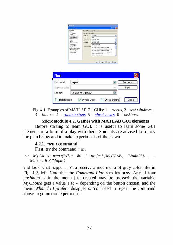
72
Micromodule 4.2. Games with MATLAB GUI elements
Before starting to learn GUI, it is useful to learn some GUI
elements in a form of a play with them. Students are advised to follow
the plan below and to make experiments of their own.
4.2.1. menu command
First, try the command menu
>> MyChoice=menu('What do I prefer?','MATLAB', 'MathCAD', …
'Matematika','Maple')
and look what happens. You receive a nice menu of gray color like in
Fig. 4.2, left. Note that the Command Line remains busy. Any of four
pushbuttons in the menu just created may be pressed; the variable
MyChoice gets a value 1 to 4 depending on the button chosen, and the
menu What do I prefer? disappears. You need to repeat the command
above to go on our experiment.
Fig. 4.1. Examples of MATLAB 7.1 GUIs: 1 – menus, 2 – text windows,
3 – buttons, 4 – radio buttons, 5 – check boxes, 6 – taskbars

73
After <Ctrl - C>, graphical object makes the Command Line free21
(don't mind error messages) but does not disappear; even several new
such menus may be run in such a way. Try: it is supposed you cannot
change size of them at the moment.
Now, play with the command gcf (Get Current Figure): different
integers will be obtained with regard to the menu to be chosen current.
These integer numbers are handles to particular existed objects. By the
command like
>> set( 2, 'color' , 'yellow')
where 2 is handle of a particular Figure, you can set a color you wish to
the menu you wish22
.
21
This is true for the version 6.* while MATLAB v.7.* behaves in a different
way. 22
Function set was already used in listing 2.3.
Fig. 4.2. Two graphical objects created by menu
command. Colors and dimensions may be changed by set.

74
How could we address a particular object? What properties are we
able to change, and how to do this? As we know handles to each object,
the command >> get(IntegerNumber)
brings to light a long list of properties and their current values relevant
to the object with the handle=IntegerNumber. You are advised to try
next games with them by the command set:
1. Change color of any menu: >> set(3,'color',yellow')
2. Change the name of one of your menus, for example >> set(2, 'Name', 'My discovery')
You cannot see the new title My discovery in full, don't you? Go on!
3. Re-switch the property Resize from off to on: >> set(2, 'Resize', 'on' )
You can change size of your rectangle menu by means of mouse now!
4. And a hocus-pocus at the end: by the commands >> set(3, 'Visible ', ' off ')
>> set(3, 'Visible ', ' on ')
your graphical object number 3 will disappear and appear again!
That's all for the menu. Feel free to make experiments of your
own with graphical objects! However, how to know values to assign to a
particular property, for instance for Pointer? The command set with no
value shall prompt you:
>> set(1, ' Pointer ')
With only handle, the command displays the whole list of values,
>> set(1)
There is a broad freedom in controlling your graphical properties. Feel
free to make experiments with also properties TooltipString, Pointer,
etc. Only read-only properties cannot be accessed.
4.2.2. uicontrol commands
Many names of commands in our focus start with ui what
abbreviates the words User Interface. Like before, it is also useful to
play with the command uicontrol and investigate its capabilities in such
way.
1. Big number of MATLAB' experiments is possible with the
syntax
75
figure(FigNo); FigNoControlNo = uicontrol(' Style ', 'ControlStyle ')
that creates an "empty" Figure with the number FigNo and with a
Control that may be one of the styles listed and briefly explained in the
table:
Style of a control Brief explanation
checkbox A rectangle for making choice yes or not by
mouse
edit Provides a field for editable text
frame A rectangle to visually group some items
listbox Control to display a list of items defined by uses
popupmenu To display a list of choices user wishes
pushbutton Button that simulates pressing and depressing
radiobutton Similar to checkbox
slider Provides a sliding bar
text Rectangle with an unchangeable (static) text
toggle Control to execute callback when clicked
For example, create Figure 5 with pushbutton that gets its handle
Fig5Obj1 (it doesn't matter what of the numeric value it gets):
>> figure(5 ), Fig5Obj1 = uicontrol( ' Style ' , ' pushbutton ')
It doesn't matter what of the numeric value the handle gets; it is more
important to be able to get properties of this first object in the Figure 5:
>> get(Fig5Obj1)
Note that controls of different style have different properties!
Particularly, find the way to manage dimensions and position of your
controls.
2. Learn what properties the above controls have, and try to
manage them. For example, the following command sets green color to
the above pushbutton:
>> set(Fig5Obj1 ,' BackgroundColor ', ' green ')
The next command superscribes the word Start by font size defined by
second pair of arguments:
>> set(Fig5Obj1 , ' String ' , ' Start ',' Fontsize ', 10)
No matter how many properties are set by a single command set at once.

76
3. Having created several Figures, try to distinguish their handles
from that of controls they have. Handles of Figures allow controlling
their properties. Say, the default colour of the Figure 5 may be changed:
>> set(5, ' color ', 'white ')
Try also to change properties of particular control in particular Figure.
4. Students are advised to investigate themselves other MATLAB
commands for creating user interfaces, such as:
uigetfile, uigetdir, helpdlg, uisetcolor, uisetfont,
h=waitbar(.3,'title','CloseRequestFcn','delete(h)'),
questdlg, msgbox, warndlg, errordlg.
Micromodule 4.3. guide, MATLAB GUI developer
The commands you learned over may help you in creating your
own graphical user interfaces to applied programs of your own.
However, you are advised to use the command guide that implements
them to facilitate such your work. MATLAB will thus make your work
easier and much less time consuming than if you would work with C++
or Java.
Calling this program from the Command Line results first in
appearance of a pilot window Quick Start that allows you to choose
from several pre-formatted GUI templates (with UIcontrols, with Axes
and Menu, and with a ready Modal Question Dialogue), Fig. 4.3.
However, start with a Blank GUI template now.
A GUI Layout Editor appears. It consists of resizable GUI Layout
Area (see Fig. 4.4) with a mesh for aligning objects, horizontal set of
instruments at the top (labelled as A, …, D) and vertical component
palette on the left with all possible GUI components (numbered here
from 1 to 11 and explained in caption below). Note that pointing mouse
cursor to any instrument icon or GUI Component (without pressing
them) results in displaying a hint what the icon serves to.
Press any component 1 to 11 in the Component Palette and drag it
in the Layout Area. In the Fig. 4.4 all kinds of UI controls have been
placed in the Layout Area, one of each kind, to demonstrate how they
look like. The grid is to align controls with respect to each other. If you
find that the Layout Area is too small, resize it by mouse cursor and the
Figure Resize Tab.

77
Double click any control in the Layout Area (or activate it and
press the Property Editor icon labelled as C in the Fig. 4.4) to call
out Property Inspector. Its particular values like self evident
Background Color, Font Name, Font Size allow to simply change
properties of the correspondent UI control. Esthetical feeling is required
to make this part of the work.
All the controls in the Layout Area are "dead" at this stage. Press
Run Button D, , to activate the GUI. You will be asked first about
the name to save it; the name TestGUI is suggested. A real GUI, an
object TestGUI.fig (with extencion .fig) has been created23
with already
"alive" GUI controls that simulate pushing or toggling buttons 1 and 2,
enabling or disabling check box 3 and radio button 4, inputting text or
numerals in the Edit Window 5, sliding in 7 and unfolding the list box 9
and pop-up menu 10, see Fig. 4.5. However, they do not do any useful
work but rather simulate it. Axes 11 do not display any useful
information as well. To do any useful actions, callbacks are to be
associated with the UI controls. They are to be written in m-file.
The m-file TestGUI.m appears when the Run Button D is pressed
for the first time; alternatively, it may be called by pressing icon B, ,
of the m-file Editor. It may be noted that this program has been quite
long, of about 200 lines. Let us analyze its structure.
The program begins with declaration of our function TestGUI that
links an output parameter varargout with input parameter varargin
(abbreviations from "variables of out-argument" and "variables of in-
argument"). It may be a good idea to structure this complex code in the
following way.
(I) First, there is a portion of comments with some explanations.
Look how they have been fitted to the names you introduced!
Programmer is advised to modify comments by providing
required information what his/her program serves to.
(II) Then, there are 18 lines with an initialization code that are
forbidden to edit.
23
Another way to call out the GUI already created is execution testgui from the
Command Line.

78
(III) There are also two functions TestGUI_OpeningFcn and
TestGUI_OutputFcn that you are advised not to modify as
well.
(IV) The last and most important portion of the code includes
description of all the dynamic GUI controls24
that were
designed by programmer. Some of the latter require one
function to operate with (they are Push Buttons, Toggle
Buttons, Radio Buttons and Check Boxes), another require two
functions (Edit Text, Sliders, List Boxes and Pop-Up Menus).
This is just the code portion where programmer should
provide his/her own commands the program is to execute.
All this is illustrated by an example below.
Micromodule 4.4. An example: GUI for helicopter
Before developing GUI for any application, programmer is to
plan what UI controls the program should have to communicate with
user. Let us illustrate this by creating GUI to the program helicopter,
Example 2.1.
Recall that the program helicopter rotates a stick on PC screen,
and we may control (i) number of rotations N, (ii) direction of rotation
(either clockwise or counter-clockwise), (iii) speed of the rotation (from
slow to fast), and (iv) colour of the rotated stick. One may think the
following UI styles to fit best for providing these data to the program:
Edit Window for (i); radiobutton for (ii); slider for (iii), and pop-up
menu for (iv). Resulting GUIhelicopter program shown in the Figure 4.6
has been made through the following stages.
1. UI control of the Static Text style was located on the Layout
Area to make title of the future program. After doing this, double click
on the newly created control, or press the Property Editor icon C, and
(a) choose Background Color you like; (b) input title you'd like to see
instead of predefined String = Static Text, for example "My first GUI:
Rotation of a stick. Input information required to Start". It is
important to make this title clearly understandable for users
prospected! The programmer is able also to specify (c) FontSize and
FontName (14 for MS Sans Serif were chosen as well as
ForegroundColor= white).
24
i.e. Static Text controls are not present here.

79
2. Make Axes Window and align it with the previous control. Call
the Property Editor and note how many properties has this control!
XTickLabel and YTickLabel properties may be set from default values
to empty in our case. Many of them may be set later.
3. Create PushButton and, by calling the Property Editor for it,
specify its color, String ("Start" was used) and FontSize were
specified such as at the stage 1. In contrast to previous steps,
providing name for the Tag (or noting its default name like
pushbuttonN) is required to find it in corresponding m-file later. In our
case, the name PushButtonStart was associated with Tag.
4. It is useful to provide titles for controls introduced on below
stages to explain them. The following Static Text controls were used:
"Number of rotations", "Direction of rotation", "Choose color of the
Stick" and "Speed of rotation".
5. For inputting N, the number of rotations, locate Edit Text
Window on the Layout Area below Axes. As before, specify
properties controlled by Property Editor. Especially important is to
assign a proper name to Tag; we set the Tag to EditN.
6. Place radio button nearby, specify text on its panel and,
especially important, set its Tag to, say, RadioButtonDirection.
7. Copy the last pair of controls (i.e. highlight it, <Ctrl-C> and
<Ctrl-V>), align the new pair on the Layout Area but change their
properties: title the Static Text String as "Choose color of the Stick",
change the Style property of the radio button control to
Style=popupmenu. The Tag was named as PopUpColor. It is
important specifically for pop-up menus: in the String box several
lines were written to list possible colors of the stick: Red, Green,
Yellow, Blue, Black, Magenta.
8. Finally, place Slider and Static Text "Speed of rotation" below
the slider, name its Tag as SliderSpeed. Important specifically for
sliders: Min and Max properties may be set from their default values
(0.0 and 1.0) to another ones. Design of the GUI GUIhelicopter has
been completed. Save all the changes under this name by pressing Run
Button D. Graphical structure of all the components implemented here
may be overviewed by pressing Object Browser D, .
Now, links between all the components chosen for the new
program are to be provided, and callbacks specified. The m-file Editor

80
with the m-file GUIhelicopter.m appeared when the Run Button E was
pressed for the first time. It may be also called by pressing icon B, .
The IV part of the generated program GUIhelicopter.m see in the
Attachment A2. Go on with the new program!
9. In the IV part of the GUIhelicopter.m code find the function
responsible for the push button. Accounting for the Tag we provided
for it on the stage 3, it has been the function
PushButtonStart_Callback. At the moment, this function contains no
commands except comments. Let us write down and store the
following piece of code taken from the program helicopter but
modified:
N=5; Direction=1; ColorText='red ';
% global N Direction Speed
Dt= Direction*pi/20;
for t=0 : Dt : Direction*2*N*pi
x1=cos(t); y1=sin(t);
x2= - x1; y2= - y1;
Pl=plot([x1, x2], [y1, y2]);
set(Pl, 'linewidth ',4); set(Pl, 'Color ',ColorText)
set(Pl, 'linewidth ',4)
axis([-1.1 1.1 -1.1 1.1]) %Constant Scales!
set(gca,'XTick', [ ]); set(gca,'yTick ', [ ])
Fig. 4.3. Pilot window after calling guide.

81
hold on; plot([0],[0],'o'); hold off; % Symbol and Color of Center Point
pause(.1) % Speed of Rotations
% pause(.1/Speed) % Speed of Rotations modified
end
You may examine that our GUI program starts working: pressing
button Start results in appearance of a stick that rotates. At this stage,
however, rotation of the stick and its color do not depend on data in
other UI controls. For example, symbol N in the window "Number of
rotations" may be substituted for, say, 100, but stick will anyway
rotate N=5 times as this has been prescribed by the first command.
10. Find now two functions responsible for the above editable text.
They are the functions EditN_CreateFcn and EditN_Callback in the
code as this determines by the Tag set on the stage 5. The second
function seems to be responsible for the callback. Two ready hints in
its comments suggest to place following commands here global N
Ntext=get(hObject,'String');
N=str2double( get( hObject,'String' ));
The second command accesses the property String of the current
object and assigns to it symbols introduced in the window. The next
command converts these symbols (they are so to be numerals!) into
the number. The first command declares the introduced N to be global.
Finally, declaration global N should be also introduced in the code of
previous stage 9: simply comment its first row and uncomment the
second. An exchange of N between two sub-programs has been
managed in such a way. Now, the stick will make as much revolutions
as user may wish.
11. A hint in the function RadioButtonDirection_Callback
associated with our radio button accordingly stage 6 suggests the
following commands to place there: global Direction
Direction=(-1)^get(hObject,'Value');
The second command produces a number Direction equal either +1 or -1
depending on the radio button is labeled or not. This number is global both
for the current function and for the code written on stage 9.
12. Similar to the stage 10, there are also two functions
PopUpColor_CreateFcn and PopUpColor_Callback responsible for
choosing color of the stick accordingly to the Tag set on the stage 7.
The last one is suggested to be extended by commands

82
global ColorText
contents = get(hObject, 'String');
ColorText=contents{get(hObject, 'Value')};
The second command returns to variable all the contents of the
String, but the third one gets the value selected from the pop-up
menu. Again, the latter should be declared global here and in the
code of the stage 9.
13. It is high time now to control speed of the rotation. In the
function SliderSpeed_Callback that provides callback of the slider,
write commands global Speed
Speed=get(hObject,'Value')+.001;
that account for hints in comments there. The second command gets
numeric value relevant to position of the slider. Note that default
values for Min=0 and Max=1 have been not changed. This value is
Fig. 4.4. GUI Editor with UI controls in the Layout Area:
A – Property Editor icon, B – Run icon; 1 – Push Button and its
icon; 2 – Toggle Button; 3 – radio Button; 4 – Check box; 5 –
Editable Text Box; 6 – Static Text; 7 – Slider; 8 – Frame; 9 – List
box; 10 – Pop-Up Menu; 11 – Axes.
Layout area
Figure
Resize Tab
C 1
2
11
11
7 8
5
3 4
E
D
9 10
B
A
D

83
passed to the function PushButtonStart_Callback explained on the
stage 9; it is suggested to uncomment the command before last.
At last, the graphical program GUIhelicopter has been completed.
Execute the command GUIhelicopter from the Command Line and type
in data it asks for. The program works fine. Figure 4.6 illustrates how
the program works. Enjoy!
Conclusion
Before shaking hands, few words should be told to conclude. You
learned MATLAB from the two viewpoints, as a mathematical
environment in Modules 1 and 3, and as a programming tool in Modules
2 and 4. These both parts equally constitute this wonderful software and
Fig. 4.5. Activated GUI shown in the Fig. 4.4. Each type of UI
controls has been represented here. However, the UI controls
"simulate" rather than execute a real work yet.

84
make it indispensable in your study and future profession of information
technology, IT. Because of volume restriction, we touched only few
aspects of this very advanced and powerful program. It is our hope that
you go on in mastering MATLAB and programming with it.
Problems for the Module 4
4.1. Give an example of soft you like and describe what of GUI it has.
4.2. Learn yourselves what perspectives in customizing your MATLAB
GUIs may be provided by commands uigetfile, uigetdir, helpdlg,
uisetcolor, uisetfont, waitbar, questdlg, msgbox, warndlg, errordlg.
4.3. Design a GUI program that creates propeller (1.9), fills it in with a
specified color and rotates in one or opposite direction a specified
number of times. Hints: use plot rather than ezplot and command fill;
a subprogram for converting coordinates (x,y) to ones (x',y') rotated
at an angle might be useful.
Figure 4.6. Graphical program GUIhelicopter that revolves stick of a
chosen color N times in clockwise or opposite direction at a given speed.

85
4.4. Design a GUI program that creates a polygon with N vertices, fills it
in with a color and rotates at various speeds (GUI shell to problem
2.10).
4.5. Develop a GUI program that asks for a function of one variable,
finds its derivative and compares graphs of both (compare with
problem 2.17).
4.6. Develop a GUI shell for program limit1 (listing 3.1) that asks for a
infinite numeric sequence like in problems 3.1 – 3.3, investigates
existence of its limit and finds the latter if any.
4.7. Develop GUI program to demonstrate how Taylor series (Fourier
series) may approximate their origin function (note the so called
Gibbs phenomenon at discontinuity points in Fourier case), problems
3.4 – 3.7.
References
1. Ануфриев И. Самоучитель MatLab 5.3/6.x. – СПб.: БХВ-
Петербург, 2002. – 736 с.
2. Гаєв Є.О., Нестеренко Б.М. Універсальний математичний пакет
MatLab і типові задачі обчислювальної математики.
Навчальний посібник. К., 2004. – 175 с.
3. Гаєв Є.О., Нестеренко Б.М. Типові задачі обчислювальної
математики з застосуванням пакету MatLab. Методичні
вказівки до виконання лабораторних робіт. К., 2004. – 38 с.
4. Демидович В.П., Марон И.А. Основы вычислительной
математики. – М.: Наука, 1966. – 664 с.
5. Денисюк В.П., Репета В.К., Гаєва К.А., Клешня Н.О. Вища
математика. Навч. посіб., ч. 3. К.: НАУб 2006. – 444с.
6. Кетков Ю., Кетков А. MatLab 6.х: программирование
численных методов. Спб: БХВ, 2004. 672 с.
7. Пайтген Х.-О., Рихтер П.Х. Красота фракталов. – Москва:
Мир, 1993. 176 с.
8. Павловский В.И. Структуры данных. Представление и
использование. – Чернигов: ЧГТУ, 2003. – 233 с.
9. Aho A.V., Hopkroft J.E., Ulman J.D. Data structures and
algorithms. (Russian translation: Ахо А.В., Хопкрофт Д.Э.,
Ульман Д.Д. Структуры данных и алгоритмы. – Москва-Киев:
Изд. дом. "Вильямс", 2003. – 384 с.)

86
10. Austin M., Chancogne D. Introduction to Engineering
Programming: in C, MATLAB, and Java. John Wiley&Sons, Inc.,
1999.
11. Azemi A., Yaz E. E. Using graphical user interface capabilities of
MATLAB in advanced engineering courses, The 38th IEEE
Conference on Decision and Control (CDC), IEEE, pp 359-363,
Phoenix, December 7-10, 1999.
12. Cooper J. A MATLAB companion for multivariable calculus. – San
Diego: Harcourt, 2001. – 294 pp.
13. Depcik Ch., Assanis D.N. Graphical User Interfaces in an
Engineering Educational Environment. CAEE2005, v13, №1, pp.48-
59.
14. Herniter M. E. Programming in MATLAB. Thomson Engineering,
2001
15. Rojan Yu. Learn Programming and Mathematics with MATLAB.
16. Tuck M. The Real History of the GUI. http://www.sitepoint.com/
article/ real-history-gui
17. Wikipedia, Graphical User Interface. http://en.wikipedia.org/wiki/
Graphical_user_ interface
18. Wirt N. (Вирт Н. Алгоритмы и структуры данных. СпБ..: Изд-во
"Невский диалект", 2001. – 352 с.)
19. Gayev Ye.A., Nesterenko B.N. MATLAB for Math and
Programming: Textbook. – Zaporozhye: Polygraph, 2006 – 102 p.
20. Азарсков В.М., Гаєв Є.О. Сучасне програмування. Модулі 1,2:
“Програмування та математика із другом MATLABом”. К.:
НАУ, 2014. – 256 с.
21. Гаєв Є.О., Рожок О., Овчарчин Н. Звук та музика в курсі
програмування. -- Інженерія програмного забезпечення, 2014,
(у друку).
22. Гаев Е.А., Мартич М., Тарак Г. Программы моделирования
случайных явлений для изучения программирования и
математики. – Інформаційні технології в освіті, 2015, (в печати)

87
Attachment A1 Listing of "MyDiff.m"
function [P,X1]=MyDiff(X,Y)
% Return Derivative of the table function Y=Y(X)
% provided length(X)=length(Y).
% Copyright Ye.Gayev
% (example of switch …case… end to compare with listing 2.2).
Nx=length(X); Ny=length(Y);
switch Nx==Ny
case 0
disp('Error: Lengths of arguments X and Y must be equal!');
case 1
disp('Differentiation has been completed!');
disp('Call "plot(X1,P)" to plot the derivative.');
X1=X(1 : end-1); % Coordinates of the derivative P(x)
X2=X(2 : end); dX=X2-X1;
Y1=Y(1 : end-1); Y2=Y(2 : end); dY=Y2-Y1;
P=dY ./ dX;
otherwise
% Nothing else except two above cases considered may happen
end
Attachment A2 Listing of "GUIhelicopter.m"
function varargout = GUIhelicopter(varargin) % Portions I to III of this program generated by MATLAB automatically
% has been skipped as they have been not the objects to edit
% Portion IV of the program:
% strings of code added by authors are written bold
%--- Executes on button press in PushButtonStart.
function PushButtonStart_Callback(hObject, eventdata, handles)
% hObject handle to PushButtonStart (see GCBO)
% eventdata reserved - to be defined in a future version of MATLAB
% handles structure with handles and user data (see GUIDATA)
%N=5; Direction=1; ColorText='red';
global N Direction ColorText Speed
%ColorText
Dt=Direction*pi/20; % Determines speed of Rotations
for t=0:Dt:Direction*2*N*pi
x1=cos(t); y1=sin(t);
x2=-x1; y2=-y1;

88
% Pl=plot([x1, x2], [y1, y2], ColorText); set(Pl, 'linewidth',4)
% Colour of the Helicopter = Red now
Pl=plot([x1, x2], [y1, y2]); set(Pl, 'linewidth',4); set(Pl, 'Color',ColorText)
axis([-1.1 1.1 -1.1 1.1]) %Constant Scales!
set(gca,'XTick', [ ]); set(gca,'yTick', [ ])
hold on; plot([0] , [0],'o'); hold off; % Symbol and Colour of Centre Point
pause(.1/Speed) % Speed of Rotations
end
% --- Executes during object creation, after setting all properties.
function EditN_CreateFcn(hObject, eventdata, handles)
% hObject handle to EditN (see GCBO)
% eventdata reserved - to be defined in a future version of MATLAB
% handles empty - handles not created until after all CreateFcns called
% Hint: edit controls usually have a white background on Windows.
% See ISPC and COMPUTER.
if ispc
set(hObject,'BackgroundColor','white');
else
set(hObject,'BackgroundColor',get(0,'defaultUicontrolBackgroundColor'));
end
function EditN_Callback(hObject, eventdata, handles)
% hObject handle to EditN (see GCBO)
% eventdata reserved - to be defined in a future version of MATLAB
% handles structure with handles and user data (see GUIDATA)
% Hints: get(hObject,'String') returns contents of EditN as text
% str2double(get(hObject,'String')) returns contents of EditN as a double
global N
Ntext=get(hObject,'String');
N=str2double(get(hObject,'String'));
% --- Executes on button press in RadioButtonDirection.
function RadioButtonDirection_Callback(hObject, eventdata, handles)
% hObject handle to RadioButtonDirection (see GCBO)
% eventdata reserved - to be defined in a future version of MATLAB
% handles structure with handles and user data (see GUIDATA)
% Hint: get(hObject,'Value') returns toggle state of RadioButtonDirection
global Direction
Direction=(-1)^get(hObject,'Value');

89
% --- Executes on selection change in PopUpColor.
function PopUpColor_Callback(hObject, eventdata, handles)
% hObject handle to PopUpColor (see GCBO)
% eventdata reserved - to be defined in a future version of MATLAB
% handles structure with handles and user data (see GUIDATA)
% Hints: contents = get(hObject,'String') returns PopUpColor contents as cell array
% contents{get(hObject,'Value')} returns selected item from PopUpColor
global ColorText
contents = get(hObject,'String');
ColorText=contents{get(hObject,'Value')};
% --- Executes during object creation, after setting all properties.
function SliderSpeed_CreateFcn(hObject, eventdata, handles)
% hObject handle to SliderSpeed (see GCBO)
% eventdata reserved - to be defined in a future version of MATLAB
% handles empty - handles not created until after all CreateFcns called
% Hint: slider controls usually have a light gray background, change
% 'usewhitebg' to 0 to use default. See ISPC and COMPUTER.
usewhitebg = 1;
if usewhitebg
set(hObject,'BackgroundColor',[.9 .9 .9]);
else
set(hObject,'BackgroundColor',get(0,'defaultUicontrolBackgroundColor'));
end
% --- Executes on slider movement.
function SliderSpeed_Callback(hObject, eventdata, handles)
% hObject handle to SliderSpeed (see GCBO)
% eventdata reserved - to be defined in a future version of MATLAB
% handles structure with handles and user data (see GUIDATA)
% Hints: get(hObject,'Value') returns position of slider
% get(hObject, 'Min') and get(hObject,'Max') to determine range of slider
global Speed
% Min=get(hObject,'Min'), Max=get(hObject,'Max'),
Speed=get(hObject,'Value')+.001;
% --- Executes during object creation, after setting all properties.
function PopUpColor_CreateFcn(hObject, eventdata, handles)
% hObject handle to PopUpColor (see GCBO)
% eventdata reserved - to be defined in a future version of MATLAB

90
% handles empty - handles not created until after all CreateFcns called
% Hint: listbox controls usually have a white background on Windows.
% See ISPC and COMPUTER.
if ispc
set(hObject,'BackgroundColor','white');
else
set(hObject,'BackgroundColor',get(0,'defaultUicontrolBackgroundColor'));
end
% End of the program GUIhelicopter
Attachment A3 Listing of "MyClock.m"
%Program, that makes arrow-hands of a clock,
% synchronised with your Windows-clock.
% The Clock will run infinitely.
%To stop it, press <Ctrl+C>
%Copyright Kornilov V.I., FCS-110 of NAU, Kyiv, December 2005
for i=1 : inf
warning off MATLAB:divideByZero;
time=fix(clock);
ezplot('x^2+y^2=25'), hold on, axis equal; axis([-6 6 -6 6]), title(datestr(now));
marksFi=[0 : pi/6 : 2*pi];
marksRho=[0 : 1 : 12].*0+5;
marksRho2=[0 : 1 : 60].*0+5;
marksFi2=[0:pi/30:2*pi];
plot(marksRho.*cos(marksFi), marksRho.*sin(marksFi), 'kh');
plot(marksRho2.*cos(marksFi2), marksRho2.*sin(marksFi2), 'm.')
plot(0, 0, 'ko')
FiH=[pi/2 pi/2 -pi/20+pi/2 pi/2 pi/20+pi/2 pi/2 pi/2]-((pi/6)*time(4))-
((pi/6)*(time(5)/60));
RhoH=[0 3 3 4 3 3 0];
xH=RhoH.*cos(FiH);
yH=RhoH.*sin(FiH);
fill(xH,yH,'r'), %pause(.01);
FiM=[pi/2 pi/2 -pi/32+pi/2 pi/2 pi/32+pi/2 pi/2 pi/2]-((pi/30)*time(5))-
((pi/30)*(time(6)/60));
RhoM=[0 2 2 5 2 2 0];
xM=RhoM.*cos(FiM);
yM=RhoM.*sin(FiM);
fill(xM,yM,'c'), %pause(.01);

91
FiS=[pi/2 pi/2 -pi/64+pi/2 pi/2 pi/64+pi/2 pi/2 pi/2]-(pi/30)*time(6);
RhoS=[0 1 1 5 1 1 0];
xS=RhoS.*cos(FiS);
yS=RhoS.*sin(FiS);
fill(xS,yS,'b'), hold off, pause(1);
WatchArr(:,i) = getframe;
end;

92
Summary of MATLAB commands
Command name
Explanation
Page
asin
atan
axis
\bf
cftool
clear
clock
collect
comet
cos
<Ctrl+C>
<Ctrl+V>
date
det
diag(x)
diff
arcsin(x)
arctg(x)
scaling and appearance of axes
example of LaTeX representation
of a symbolic expression
separate Curve Fitting Tool
Clearing variables from memory
Getting current date and time
Collecting coefficients of symbolic
expression
Plotting comet-like trajectory
cos(x)
COPY hotkey, or breaking
execution if computer hangs
PASTE hotkey
Getting current date
|| A , determinant of square matrix
diagonal square matrix with the
elements from x
differentiation, either numeric
vector of symbolic function
23
22
13,14,35,42,81,89
54,55,59
64
54,66
26,38,39
19
14,26
35,73,79,91
79
26
19,23
14
21

93
disp
else
elseif
end
expand
eval
eye
ezplot
ezsurf
false
figure
fill
for
format
fplot
function
fzero
displays content of argument
key words of if … end statement
condition
key word of array last element
number, or end of a structural for-,
while-, if- etc. blocks
removes brackets of products of
symbolic expressions
evaluates string as MATLAB
expression and executes it
producing Identity matrix
easy-to-use plotting commands in
2 and 3 dimensions
logical zero, 0
create new figure window
creation of 2d polygon filled by a
specified colour
key word of execution loop
setting format of outputting
numeric data
easy-to-use 2d plotting
key word for be adding a new
command to MATLAB's
vocabulary
tries to find a zero of a function if
an initial guess is provided
38,43-50,58-61,88
35,37-40,54,89-91
18,19
22,23
10
13,15,20-22,37,49,59
34,39-41,44
13,22,28,49,63,75
15,51,84
34,35,43,45-47,46
13,26,38,42,51,59
29,31,37,41,43,45-47
23

94
gcf
get
global
grid
guide
help
i
if
inf
input
int
inv
j
legend
length
max
menu
getting handle to current figure
getting properties of an object
declaration for exchange by
variables between programs
drawing grid lines on a plot
program for designing GUI
enquiring HELP from command
line
1
key word of conditional program
block
MATLAB's notation of
prompting for user input
command for integrating symbolic
function
calculate inverse matrix
1
puts legends of current plotted
curves
determination of vector length
determines largest component of
vector argument, or property of a
Figure object
generates Figure with a menu of
choices
73
73,75,81-83,89,90
32,33,81-83,88-90
26,28
76
10,11,30,34,37
8
34-40,43-45,54,89-91
48,49,54,58
24
8
24,67
12,43,45,46,62,88
46,80,83,90
71-75

95
min
NaN
ones
pause
pi
plot
plot3
poly
poly2sym
polyval
pretty
rand
randn
roots
round
set
determines smallest component of
vector argument, or property of a
Figure object
Not-a-Number, results of
mathematically undefined
operations
matrix with only 1s
pauses program execution
3.14159...
plots vector versus vector
a three-dimensional analogue of
plot
converts vector of roots to vector
of polynomial coefficients
converts polynomial from numeric
to symbolic representation
evaluates polynomial at given x
prints symbolic expression on
screen in LaTeX form
generates random numbers
distributed uniformly or normally
finds roots of numerically
represented polynomial
rounding data towards nearest
integer
setting properties of Figures
46,80,83,90
10
35,48,49,58,89
14,28,35,42,54,62,63,6
5,67,81,88,89
21
18
19,21,23
61,62,64,66
17,18
66
35,73-76,81,89-91

96
size
sqrt
solve
subs
sum
switch
sym, syms
sym2poly
taylor
text
tic
toc
title
true
uicontrol
while
returns both dimensions of
matrices
solves algebraic equation sets
symbolically or numerically
substitutes symbols in symbolic
expressions
sums elements of vector
key word of
switch…case…otherwise…end
statement
declarations of symbolic variables
converts polynomial from
symbolic to numeric representation
finds Taylor series expansion of
given symbolic function
annotating a text on Figures
starting and reading stopwatch
timer
printing title text on graphics
logical one, 1
creates user interface controls
key word of while…end statement
looping indefinite number of times
12,47
19,23
20,21,23
12
35,46,88
18,21,23,48
20
23
54
65
34,39-41
74,75
35,43,44,54

97
xlabel
ylabel
zeros
labelling Ox and Oy axes on
Figures
matrix with only zeros, 0
28,54,67
10

98
C o n t e n t s
Foreword ………………………………………………..………….3
Module 1: MATLAB, the mathematical environment………….5
Micromodule 1.1. Basics of MATLAB…………………………….5
1.1.1. Getting started……………………………………….6
1.1.2. Matrix arithmetic of the MATLAB …………………8 Micromodule 1.2. Plotting 1d functions……………………………12 Micromodule 1.3. Numeric and symbolic calculations ……………15
1.3.1. Polynomials …………………………………………..16
1.3.2. Symbolic mathematics in MATLAB …………………21
Problems for Module 1 …………………………………………….25
Module 2: Basics of MATLAB programming …………………..27
Micromodule 2.1. m-scripts and m-functions …………………..…27
2.1.1. Scripts, the simplest programs………………………....27
2.1.2. MATLAB' Functions (m-functions) …………………..29
2.1.3. Difference between Scripts and Functions …………….31
Micromodule 2.2. Structured programming in MATLAB ………….33
2.2.1. Loop operator for … end ………………………………34
2.2.2. Logical operator if … else … end ……………………...35
2.2.3. Logical arithmetic with and, or, not …………………...40
Micromodule 2.3. More MATLAB' programs ……………………...42
2.3.1. Periodic Step-function …………………………………42
2.3.2. Least element of an array ………………………………45
2.3.3. Re-ordering of a vector …………………………….…..46
Micromodule 2.4. Supplementary problems ……………………..…48
2.4.1. Dialogue programs ………………………………….…48
2.4.2. Debugging programs ……………………………….…49
Problems for Module 2 ………………………………………….…50
Module 3: MATLAB for learning and investigation …………..53
Micromodule 3.1. The awful "ε – δ language"! ……………………53
Micromodule 3.2. Taylor, Fourier… Who else? ……………………57
Micromodule 3.3. Discovering empirical formulas ………………..60
Micromodule 3.4. Efficiency of programs …………………………65
Micromodule 3.5. Your further discoveries with MATLAB………
Problems for Module 3 ………………………………………….…68

99
Module 4: Graphical User Interface in MATLAB ………………71
Micromodule 4.1. Graphical User Interface (GUI) standards ………71
Micromodule 4.2. Games with MATLAB GUI elements ………..…72
4.2.1. menu command ………………………………………...72
4.2.2. uicontrol commands ……………………………………74
Micromodule 4.3. guide, MATLAB GUI developer ……………..…76
Micromodule 4.4. An example: GUI for helicopter …………………78
Conclusion ……………………………………………………….…..83
Problems for the Module 4 …………………………………….….…84
References ……………………………………………………….…..86
Attachment A1: Listing of "MyDiff.m" ……………………….…...……88
Attachment A2: Listing of "GUIhelicopter.m" …………………...……88
Attachment A3: Listing of "MyClock.m" ………………………...……91
Summary of MATLAB commands …………………….…….……..93
100
Навчальне видання
MATLAB for Math and Programming: Textbook
MATLAB для математики та програмування: Навч. посібник
(англійською мовою)
Гаєв Євген Олександрович
Нестеренко Борис Миколайович
Перше видання підписано до друку 15.12.2006.
Друге видання, виправлене та покращене,
публікується авторами у червні 2015 р. з власної ініціативи.
Всі права захищені!
Є.О. Гаєв, Б.М. Нестеренко
Використання цієї книги вітається,
але автори мають бути повідомлені.
Author’s address
Адрес автора [email protected]