MATLAB for M151B - Texas A&M University

MATLAB for M151B

c© 2008 Peter Howard

1

MATLAB for M151B

P. Howard

Fall 2008

Contents

1 Introduction 51.1 The Origin of MATLAB . . . . . . . . . . . . . . . . . . . . . . . . . . . . . 51.2 Our Course Goal . . . . . . . . . . . . . . . . . . . . . . . . . . . . . . . . . 51.3 Starting MATLAB at Texas A&M University . . . . . . . . . . . . . . . . . 51.4 The MATLAB Interface . . . . . . . . . . . . . . . . . . . . . . . . . . . . . 51.5 Basic Computations . . . . . . . . . . . . . . . . . . . . . . . . . . . . . . . 61.6 Diary Files . . . . . . . . . . . . . . . . . . . . . . . . . . . . . . . . . . . . . 61.7 Getting Help . . . . . . . . . . . . . . . . . . . . . . . . . . . . . . . . . . . 71.8 Assignments . . . . . . . . . . . . . . . . . . . . . . . . . . . . . . . . . . . . 7

2 Symbolic Calculations in MATLAB 92.1 Defining Symbolic Objects . . . . . . . . . . . . . . . . . . . . . . . . . . . . 9

2.1.1 Complex Numbers . . . . . . . . . . . . . . . . . . . . . . . . . . . . 102.1.2 The Clear Command . . . . . . . . . . . . . . . . . . . . . . . . . . . 10

2.2 Manipulating Symbolic Expressions . . . . . . . . . . . . . . . . . . . . . . . 102.2.1 The Collect Command . . . . . . . . . . . . . . . . . . . . . . . . . . 112.2.2 The Expand Command . . . . . . . . . . . . . . . . . . . . . . . . . . 112.2.3 The Factor Command . . . . . . . . . . . . . . . . . . . . . . . . . . 122.2.4 The Horner Command . . . . . . . . . . . . . . . . . . . . . . . . . . 122.2.5 The Simple Command . . . . . . . . . . . . . . . . . . . . . . . . . . 122.2.6 The Pretty Command . . . . . . . . . . . . . . . . . . . . . . . . . . 13

2.3 Solving Algebraic Equations . . . . . . . . . . . . . . . . . . . . . . . . . . . 142.4 Numerical Calculations with Symbolic Expressions . . . . . . . . . . . . . . 16

2.4.1 The Double and Eval commands . . . . . . . . . . . . . . . . . . . . 162.4.2 The Subs Command . . . . . . . . . . . . . . . . . . . . . . . . . . . 16

2.5 Assignments . . . . . . . . . . . . . . . . . . . . . . . . . . . . . . . . . . . . 17

3 Plots and Graphs in MATLAB 183.1 The Plot Command . . . . . . . . . . . . . . . . . . . . . . . . . . . . . . . . 183.2 Plotting Functions with the plot command . . . . . . . . . . . . . . . . . . . 193.3 Parametric Curves . . . . . . . . . . . . . . . . . . . . . . . . . . . . . . . . 213.4 Juxtaposing One Plot On Top of Another . . . . . . . . . . . . . . . . . . . 21

2

3.5 Multiple Plots . . . . . . . . . . . . . . . . . . . . . . . . . . . . . . . . . . . 223.6 Ezplot . . . . . . . . . . . . . . . . . . . . . . . . . . . . . . . . . . . . . . . 233.7 Saving Plots as Encapsulated Postscript Files . . . . . . . . . . . . . . . . . 253.8 Assignments . . . . . . . . . . . . . . . . . . . . . . . . . . . . . . . . . . . . 25

4 Semilog and Double-log Plots 274.1 Semilog Plots . . . . . . . . . . . . . . . . . . . . . . . . . . . . . . . . . . . 27

4.1.1 Deriving Functional Relations from a Semilog Plot . . . . . . . . . . 294.2 Double-log Plots . . . . . . . . . . . . . . . . . . . . . . . . . . . . . . . . . 304.3 Assignments . . . . . . . . . . . . . . . . . . . . . . . . . . . . . . . . . . . . 32

5 Inline Functions and M-Files 335.1 Inline Functions . . . . . . . . . . . . . . . . . . . . . . . . . . . . . . . . . . 335.2 Script M-Files . . . . . . . . . . . . . . . . . . . . . . . . . . . . . . . . . . . 355.3 Function M-files . . . . . . . . . . . . . . . . . . . . . . . . . . . . . . . . . . 365.4 Functions that Return Values . . . . . . . . . . . . . . . . . . . . . . . . . . 375.5 Debugging M-files . . . . . . . . . . . . . . . . . . . . . . . . . . . . . . . . . 385.6 Assignments . . . . . . . . . . . . . . . . . . . . . . . . . . . . . . . . . . . . 39

6 Function Limits in MATLAB 406.1 Symbolic Limits of Functions . . . . . . . . . . . . . . . . . . . . . . . . . . 406.2 Divergence by Oscillation . . . . . . . . . . . . . . . . . . . . . . . . . . . . . 416.3 The Sandwich Theorem . . . . . . . . . . . . . . . . . . . . . . . . . . . . . 416.4 The Bisection Method . . . . . . . . . . . . . . . . . . . . . . . . . . . . . . 426.5 Experimenting with the Formal Definition of Limits . . . . . . . . . . . . . . 466.6 Assignments . . . . . . . . . . . . . . . . . . . . . . . . . . . . . . . . . . . . 47

7 Symbolic Derivatives in MATLAB 507.1 Computing Higher Order Derivatives in MATLAB . . . . . . . . . . . . . . . 507.2 Computing Derivatives as Limits . . . . . . . . . . . . . . . . . . . . . . . . 527.3 Dynamic and Geometric Interpretations of the Derivative . . . . . . . . . . . 537.4 Computing the Equation of the Tangent Line . . . . . . . . . . . . . . . . . 557.5 Assignments . . . . . . . . . . . . . . . . . . . . . . . . . . . . . . . . . . . . 57

8 Implicitly Defined Functions 588.1 Plotting Implicitly Defined Functions . . . . . . . . . . . . . . . . . . . . . . 588.2 Tangent Lines for Implicitly Defined Relations . . . . . . . . . . . . . . . . . 598.3 Implicit Differentiation in MATLAB (sort of) . . . . . . . . . . . . . . . . . 618.4 Assignments . . . . . . . . . . . . . . . . . . . . . . . . . . . . . . . . . . . . 62

9 Derivatives of Exponential and Inverse Functions 639.1 Approximating e from the Definition . . . . . . . . . . . . . . . . . . . . . . 639.2 The Derivative of an Inverse Function . . . . . . . . . . . . . . . . . . . . . . 649.3 Assignments . . . . . . . . . . . . . . . . . . . . . . . . . . . . . . . . . . . . 67

3

10 Extrema and the Mean Value Theorem 6910.1 The Mean Value Theorem . . . . . . . . . . . . . . . . . . . . . . . . . . . . 6910.2 Monotonicity . . . . . . . . . . . . . . . . . . . . . . . . . . . . . . . . . . . 7010.3 Concavity . . . . . . . . . . . . . . . . . . . . . . . . . . . . . . . . . . . . . 7110.4 Maximization and Minimization . . . . . . . . . . . . . . . . . . . . . . . . . 7210.5 Assignments . . . . . . . . . . . . . . . . . . . . . . . . . . . . . . . . . . . . 75

11 Limits of Sequences 7711.1 Experimenting with the Limit Definition . . . . . . . . . . . . . . . . . . . . 7811.2 Recursions . . . . . . . . . . . . . . . . . . . . . . . . . . . . . . . . . . . . . 79

12 Cobwebbing and Newton’s Method 8212.1 Cobwebbing . . . . . . . . . . . . . . . . . . . . . . . . . . . . . . . . . . . . 8212.2 Newton’s Method . . . . . . . . . . . . . . . . . . . . . . . . . . . . . . . . . 8512.3 Assignments . . . . . . . . . . . . . . . . . . . . . . . . . . . . . . . . . . . . 87

13 Riemann Sums in MATLAB 8813.1 Riemann Sums . . . . . . . . . . . . . . . . . . . . . . . . . . . . . . . . . . 8813.2 Assignments . . . . . . . . . . . . . . . . . . . . . . . . . . . . . . . . . . . . 92

14 Symbolic and Numerical Integration in MATLAB 9314.1 Symbolic Integration in MATLAB . . . . . . . . . . . . . . . . . . . . . . . . 9314.2 Numerical Integration in MATLAB . . . . . . . . . . . . . . . . . . . . . . . 9414.3 Assignments . . . . . . . . . . . . . . . . . . . . . . . . . . . . . . . . . . . . 95

4

1 Introduction

1.1 The Origin of MATLAB

MATLAB, which stands for MATrix LABoratory, is a software package developed by Math-Works, Inc. to facillitate numerical computations as well as some symbolic manipulation.The collection of programs (originally written in Fortran) that eventually became MATLABwere developed in the late 1970s by Cleve Moler, who used them in a numerical analysiscourse he was teaching at the University of New Mexico. Jack Little and Steve Bangertlater reprogrammed these routines in C, and added M-files, toolboxes, and more powerfulgraphics (original versions created plots by printing asterisks on the screen). Moler, Little,and Bangert founded MathWorks in California in 1984.

1.2 Our Course Goal

In recent years mathematical computations have begun to play a larger role in the biologicalsciences, and MATLAB is a useful platform for carrying out such calculations with relativeease. While our focus will naturally be on concepts that arise in calculus, and on theapplications of these concepts, it is also important that students gain some basic familiaritywith MATLAB’s capabilities as a general computing tool. In particular, we will beginthe semester with some background material on arithmetic, algebra, and graphing, andconsequently the MATLAB material will lag several weeks behind the class lecture material.For example, while we will begin with limits of functions on the first day of class, we willnot get to limits in MATLAB until Week 6.

1.3 Starting MATLAB at Texas A&M University

Your NetID and password should access your calclab account. Log in and click on the sixpointed geometric figure in the bottom left corner of your screen. Go to Mathematics andchoose Matlab. Congratulations! (Alternatively, click on the surface plot icon at the footof your screen.)

1.4 The MATLAB Interface

The (default) MATLAB screen is divided into three windows, with a large Command Windowon the right, and two smaller windows stacked one atop the other on the left. (If thesewindows aren’t maximized on your screen, you can maximize them by selecting the middlebutton at the top right corner of the MATLAB box.) The Command Window is wherecalculations are carried out in MATLAB, while the smaller windows display informationabout your current MATLAB session, your previous MATLAB sessions, and your computeraccount. Your options for these smaller windows are Command History, which displays thecommands you’ve typed in from both the current and previous sessions, Current Directory,which shows which directory you’re currently in and what files are in that directory, andWorkspace, which displays information about each variable defined in your current session.You can choose which of these options you would like to have displayed by selecting Desktop

5

from the main MATLAB window. Occasionally, it will be important that you are workingin a certain directory. Notice that you can change MATLAB’s working directory by double-clicking on a directory in the Current Directory window. In order to go backwards a directory,click on the folder with a black arrow on it in the top left corner of the Current Directorywindow.

1.5 Basic Computations

At the prompt designated by two arrows, >>, type sin(0) and press Enter. You should findthat the answer has been assigned to the default variable ans. Next, type sin(0); and hitEnter (there is now a semicolon at the end of the line). Notice that the semicolon suppressesscreen output.

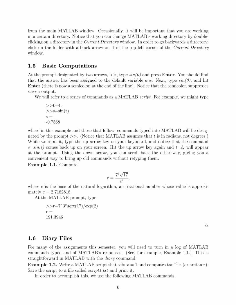
We will refer to a series of commands as a MATLAB script. For example, we might type

>>t=4;>>s=sin(t)s =-0.7568

where in this example and those that follow, commands typed into MATLAB will be desig-nated by the prompt >>. (Notice that MATLAB assumes that t is in radians, not degrees.)While we’re at it, type the up arrow key on your keyboard, and notice that the commands=sin(t) comes back up on your screen. Hit the up arrow key again and t=4; will appearat the prompt. Using the down arrow, you can scroll back the other way, giving you aconvenient way to bring up old commands without retyping them.

Example 1.1. Compute

r =73√

17

e2,

where e is the base of the natural logarithm, an irrational number whose value is approxi-mately e = 2.7182818.

At the MATLAB prompt, type

>>r=7ˆ3*sqrt(17)/exp(2)r =191.3946

△

1.6 Diary Files

For many of the assignments this semester, you will need to turn in a log of MATLABcommands typed and of MATLAB’s responses. (See, for example, Example 1.1.) This isstraightforward in MATLAB with the diary command.

Example 1.2. Write a MATLAB script that sets x = 1 and computes tan−1 x (or arctan x).Save the script to a file called script1.txt and print it.

In order to accomplish this, we use the following MATLAB commands.

6

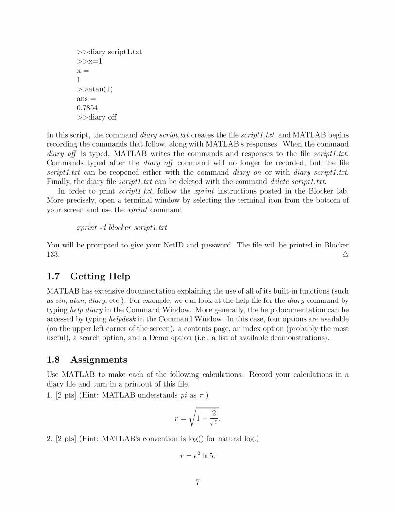
>>diary script1.txt>>x=1x =1>>atan(1)ans =0.7854>>diary off

In this script, the command diary script.txt creates the file script1.txt, and MATLAB beginsrecording the commands that follow, along with MATLAB’s responses. When the commanddiary off is typed, MATLAB writes the commands and responses to the file script1.txt.Commands typed after the diary off command will no longer be recorded, but the filescript1.txt can be reopened either with the command diary on or with diary script1.txt.Finally, the diary file script1.txt can be deleted with the command delete script1.txt.

In order to print script1.txt, follow the xprint instructions posted in the Blocker lab.More precisely, open a terminal window by selecting the terminal icon from the bottom ofyour screen and use the xprint command

xprint -d blocker script1.txt

You will be prompted to give your NetID and password. The file will be printed in Blocker133. △

1.7 Getting Help

MATLAB has extensive documentation explaining the use of all of its built-in functions (suchas sin, atan, diary, etc.). For example, we can look at the help file for the diary command bytyping help diary in the Command Window. More generally, the help documentation can beaccessed by typing helpdesk in the Command Window. In this case, four options are available(on the upper left corner of the screen): a contents page, an index option (probably the mostuseful), a search option, and a Demo option (i.e., a list of available deomonstrations).

1.8 Assignments

Use MATLAB to make each of the following calculations. Record your calculations in adiary file and turn in a printout of this file.

1. [2 pts] (Hint: MATLAB understands pi as π.)

r =

√

1 − 2

π5.

2. [2 pts] (Hint: MATLAB’s convention is log() for natural log.)

r = e2 ln 5.

7

3. [2 pts]r = sin2 2 + cos2 4,

with 2 and 4 measured in radians, MATLAB’s default.

4. [2 pts]r = sin2 30 + cos2 40,

30 and 40 measured in degrees. (This requires a conversion.)

5. [2 pts] Use MATLAB’s built-in help to look up the function lambertw. Compute w(2)and write down the equation this value solves.

8

2 Symbolic Calculations in MATLAB

Though MATLAB has not been designed with symbolic calculations in mind, it can carrythem out with the Symbolic Math Toolbox, which is standard with student versions. (Inorder to check if this, or any other toolbox is on a particular version of MATLAB, type ver atthe MATLAB prompt.) In carrying out these calculations, MATLAB uses Maple software1,but the user interface is significantly different.

2.1 Defining Symbolic Objects

Symbolic manipulations in MATLAB are carried out on symbolic variables, which can beeither particular numbers or unspecified variables. The easiest way in which to define avariable as symbolic is with the syms command.

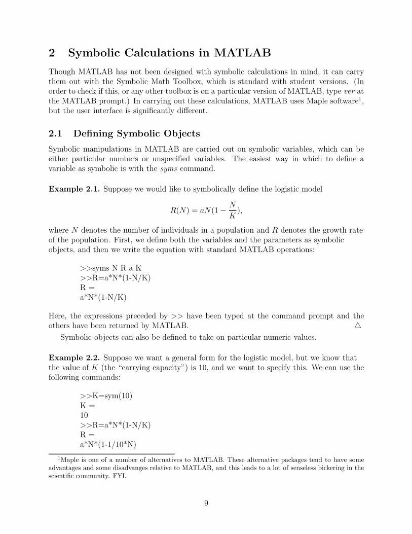
Example 2.1. Suppose we would like to symbolically define the logistic model

R(N) = aN(1 − N

K),

where N denotes the number of individuals in a population and R denotes the growth rateof the population. First, we define both the variables and the parameters as symbolicobjects, and then we write the equation with standard MATLAB operations:

>>syms N R a K>>R=a*N*(1-N/K)R =a*N*(1-N/K)

Here, the expressions preceded by >> have been typed at the command prompt and theothers have been returned by MATLAB. △

Symbolic objects can also be defined to take on particular numeric values.

Example 2.2. Suppose we want a general form for the logistic model, but we know thatthe value of K (the “carrying capacity”) is 10, and we want to specify this. We can use thefollowing commands:

>>K=sym(10)K =10>>R=a*N*(1-N/K)R =a*N*(1-1/10*N)

1Maple is one of a number of alternatives to MATLAB. These alternative packages tend to have someadvantages and some disadvanges relative to MATLAB, and this leads to a lot of senseless bickering in thescientific community. FYI.

9

2.1.1 Complex Numbers

You can also define and manipulate symbolic complex numbers in MATLAB. Recall that acomplex number has the form

z = x + iy,

where x and y are both real numbers and i =√−1. The complex conjugate of a complex

number, denoted z̄, is defined byz̄ = x − iy.

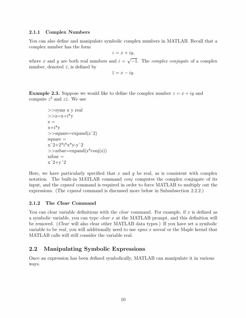
Example 2.3. Suppose we would like to define the complex number z = x + iy andcompute z2 and zz̄. We use

>>syms x y real>>z=x+i*yz =x+i*y>>square=expand(zˆ2)square =xˆ2+2*i*x*y-yˆ2>>zzbar=expand(z*conj(z))zzbar =xˆ2+yˆ2

Here, we have particularly specified that x and y be real, as is consistent with complexnotation. The built-in MATLAB command conj computes the complex conjugate of itsinput, and the expand command is required in order to force MATLAB to multiply out theexpressions. (The expand command is discussed more below in Subsubsection 2.2.2.)

2.1.2 The Clear Command

You can clear variable definitions with the clear command. For example, if x is defined asa symbolic variable, you can type clear x at the MATLAB prompt, and this definition willbe removed. (Clear will also clear other MATLAB data types.) If you have set a symbolicvariable to be real , you will additionally need to use syms x unreal or the Maple kernel thatMATLAB calls will still consider the variable real.

2.2 Manipulating Symbolic Expressions

Once an expression has been defined symbolically, MATLAB can manipulate it in variousways.

10

2.2.1 The Collect Command

The collect command gathers all terms together that have a variable to the same power.

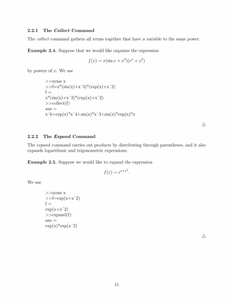
Example 2.4. Suppose that we would like organize the expression

f(x) = x(sin x + x3)(ex + x2)

by powers of x. We use

>>syms x>>f=x*(sin(x)+xˆ3)*(exp(x)+xˆ2)f =x*(sin(x)+xˆ3)*(exp(x)+xˆ2)>>collect(f)ans =xˆ6+exp(x)*xˆ4+sin(x)*xˆ3+sin(x)*exp(x)*x

△

2.2.2 The Expand Command

The expand command carries out products by distributing through parentheses, and it alsoexpands logarithmic and trigonometric expressions.

Example 2.5. Suppose we would like to expand the expression

f(x) = ex+x2

.

We use

>>syms x>>f=exp(x+xˆ2)f =exp(x+xˆ2)>>expand(f)ans =exp(x)*exp(xˆ2)

△

11

2.2.3 The Factor Command

The factor command can be used to factor polynomials.

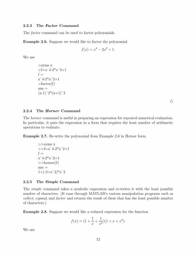
Example 2.6. Suppose we would like to factor the polynomial

f(x) = x4 − 2x2 + 1.

We use

>syms x>f=xˆ4-2*xˆ2+1f =xˆ4-2*xˆ2+1>factor(f)ans =(x-1)ˆ2*(x+1)ˆ2

△

2.2.4 The Horner Command

The horner command is useful in preparing an expression for repeated numerical evaluation.In particular, it puts the expression in a form that requires the least number of arithmeticoperations to evaluate.

Example 2.7. Re-write the polynomial from Example 2.6 in Horner form.

>>syms x>>f=xˆ4-2*xˆ2+1f =xˆ4-2*xˆ2+1>>horner(f)ans =1+(-2+xˆ2)*xˆ2

2.2.5 The Simple Command

The simple command takes a symbolic expression and re-writes it with the least possiblenumber of characters. (It runs through MATLAB’s various manipulation programs such ascollect, expand, and factor and returns the result of these that has the least possible numberof characters.)

Example 2.8. Suppose we would like a reduced expression for the function

f(x) = (1 +1

x+

1

x2)(1 + x + x2).

We use

12

>>syms x f>>f=(1+1/x+1/xˆ2)*(1+x+xˆ2)f =(1+1/x+1/xˆ2)*(x+1+xˆ2)>>simple(f)simplify:(x+1+xˆ2)ˆ2/xˆ2radsimp:(x+1+xˆ2)ˆ2/xˆ2combine(trig):(3*xˆ2+2*x+2*xˆ3+1+xˆ4)/xˆ2factor:(x+1+xˆ2)ˆ2/xˆ2expand:2*x+3+xˆ2+2/x+1/xˆ2combine:(1+1/x+1/xˆ2)*(x+1+xˆ2)convert(exp):(1+1/x+1/xˆ2)*(x+1+xˆ2)convert(sincos):(1+1/x+1/xˆ2)*(x+1+xˆ2)convert(tan):(1+1/x+1/xˆ2)*(x+1+xˆ2)collect(x):2*x+3+xˆ2+2/x+1/xˆ2mwcos2sin:(1+1/x+1/xˆ2)*(x+1+xˆ2)ans =(x+1+xˆ2)ˆ2/xˆ2

In this example, three lines have been typed, and the rest is MATLAB output as it triesvarious possibilities. It returns the expression in ans, in this case from the factor command.△

2.2.6 The Pretty Command

MATLAB’s pretty command simply re-writes a symbolic expression in a form that appearsmore like typeset mathematics than does MATLAB syntax.

Example 2.9. Suppose we would like to re-write the expression from Example 2.8 in amore readable format. Assuming, we have already defined f as in Example 2.8, we usepretty(f) at the MATLAB prompt. (The output of this command doesn’t translate wellinto a printed document, so I won’t give it here.)

13

2.3 Solving Algebraic Equations

MATLAB’s built-in function for solving equations symbolically is solve.

Example 2.10. Suppose we would like to solve the quadratic equation

ax2 + bx + c = 0.

We use

>>syms a b c x>>eqn=a*xˆ2+b*x+ceqn =a*xˆ2+b*x+c>>roots=solve(eqn)roots =1/2/a*(-b+(bˆ2-4*a*c)ˆ(1/2))1/2/a*(-b-(bˆ2-4*a*c)ˆ(1/2))

Observe that we only defined the expression on the left-hand side of our equality. By default,MATLAB’s solve command sets this expression to 0. Also, notice that MATLAB knew whichvariable to solve for. (It takes x as a default variable.) Suppose that in lieu of solving for x,we know x and would like to solve for a. We can specify this with the following commands:

>>a=solve(eqn,a)a =-(b*x+c)/xˆ2

In this case, we have particularly specified in the solve command that we are solving for a.Alternatively, we can type an entire equation directly into the solve command. For example:

>>syms a>>roots=solve(a*xˆ2+b*x+c)roots =1/2/a*(-b+(bˆ2-4*a*c)ˆ(1/2))1/2/a*(-b-(bˆ2-4*a*c)ˆ(1/2))

Here, the syms command has been used again because a has been redefined in the codeabove. Finally, we need not first make our variables symbolic if we put the expression insolve in single quotes. We could simply use solve(’a*xˆ2+b*x+c’). △

MATLAB’s solve command can also solve systems of equations.

Example 2.11. For a population of prey x with growth rate Rx and a population ofpredators y with growth rate Ry, the the Lotka–Volterra predator–prey model is

Rx = ax − bxy

Ry = − cy + dxy.

14

In this example, we would like to determine whether or not there is a pair of populationvalues (x, y) for which neither population is either growing or decaying (the rates are both0). We call such a point an equilibrium point. The equations we need to solve are:

0 = ax − bxy

0 = − cy + dxy.

In MATLAB

>>syms a b c d x y>>Rx=a*x-b*x*yRx =a*x-b*x*y>>Ry=-c*y+d*x*yRy =-c*y+d*x*y>>[prey pred]=solve(Rx,Ry)prey =01/d*cpred =01/b*a

Again, MATLAB knows to set each of the expression Rx and Ry to 0. In this case, MAT-LAB has returned two solutions, one with (0, 0) and one with ( c

d, a

b). In this example, the

appearance of [prey pred] particularly requests that MATLAB return its solution as a vectorwith two components. Alternatively, we have the following:

>>pops=solve(Rx,Ry)pops =x: [2x1 sym]y: [2x1 sym]>>pops.xans =01/d*c>>pops.yans =01/b*a

In this case, MATLAB has returned its solution as a MATLAB structure, which is a dataarray that can store a combination of different data types: symbolic variables, numericvalues, strings etc. In order to access the value in a structure, the format is

structure name.variable identification △

15

2.4 Numerical Calculations with Symbolic Expressions

In many cases, we would like to combine symbolic manipulation with numerical calculation.

2.4.1 The Double and Eval commands

The double and eval commands change a symbolic variable into an appropriate double vari-able (i.e., a numeric value).

Example 2.12. Suppose we would like to symbolically solve the equation x3 + 2x − 1 = 0,and then evaluate the result numerically. We use

>>syms x>>r=solve(xˆ3+2*x-1);>>eval(r)ans =0.4534-0.2267 + 1.4677i-0.2267 - 1.4677i>>double(r)ans =0.4534-0.2267 + 1.4677i-0.2267 - 1.4677i

MATLAB’s symbolic expression for r is long, so I haven’t included it here, but you shouldtake a look at it by leaving the semicolon off the solve line. △

2.4.2 The Subs Command

In any symbolic expression, values can be substituted for symbolic variables with the subscommand.

Example 2.13. Suppose that in our logistic model

R(N) = aN(1 − N

K),

we would like to substitute the values a = .1 and K = 10. We use

>>syms a K N>>R=a*N*(1-N/K)R =a*N*(1-N/K)>>R=subs(R,a,.1)R =1/10*N*(1-N/K)>>R=subs(R,K,10)R =1/10*N*(1-1/10*N)

16

Alternatively, numeric values can be substitued in. We can accomplish the same result asabove with the commands

>>syms a K N>>R=a*N*(1-N/K)R =a*N*(1-N/K)>>a=.1a =0.1000>>K=10K =10>>R=subs(R)R =1/10*N*(1-1/10*N)

In this case, the specifications a = .1 and K = 10 have defined a and K as numeric values.The subs command, however, places them into the symbolic expression.

2.5 Assignments

For each problem, turn in a diary file containing your MATLAB script along with MATLAB’soutput.

1. [2 pts] Factor the polynomial

x5 − 15x4 + 85x3 − 225x2 + 274x − 120.

2. [2 pts] Find an inverse for the function

f(x) =1 − x

1 + x; x 6= −1.

3. [2 pts] Solve the equation

x − y

x− y2 = 0

for y as a function of x. (Hint. This is a good problem to use the pretty command on.)4. [2 pts] Find all solutions for the system of algebraic equations

x2 − y2 = 0

2y − x = 1.

5. [2 pts] Write down expressions for the three solutions for

ax3 + c = 0.

Use the subs command to evaluate your solution for a = 1 and c = 2.

17

3 Plots and Graphs in MATLAB

3.1 The Plot Command

The primary tool we will use for plotting in MATLAB is plot().

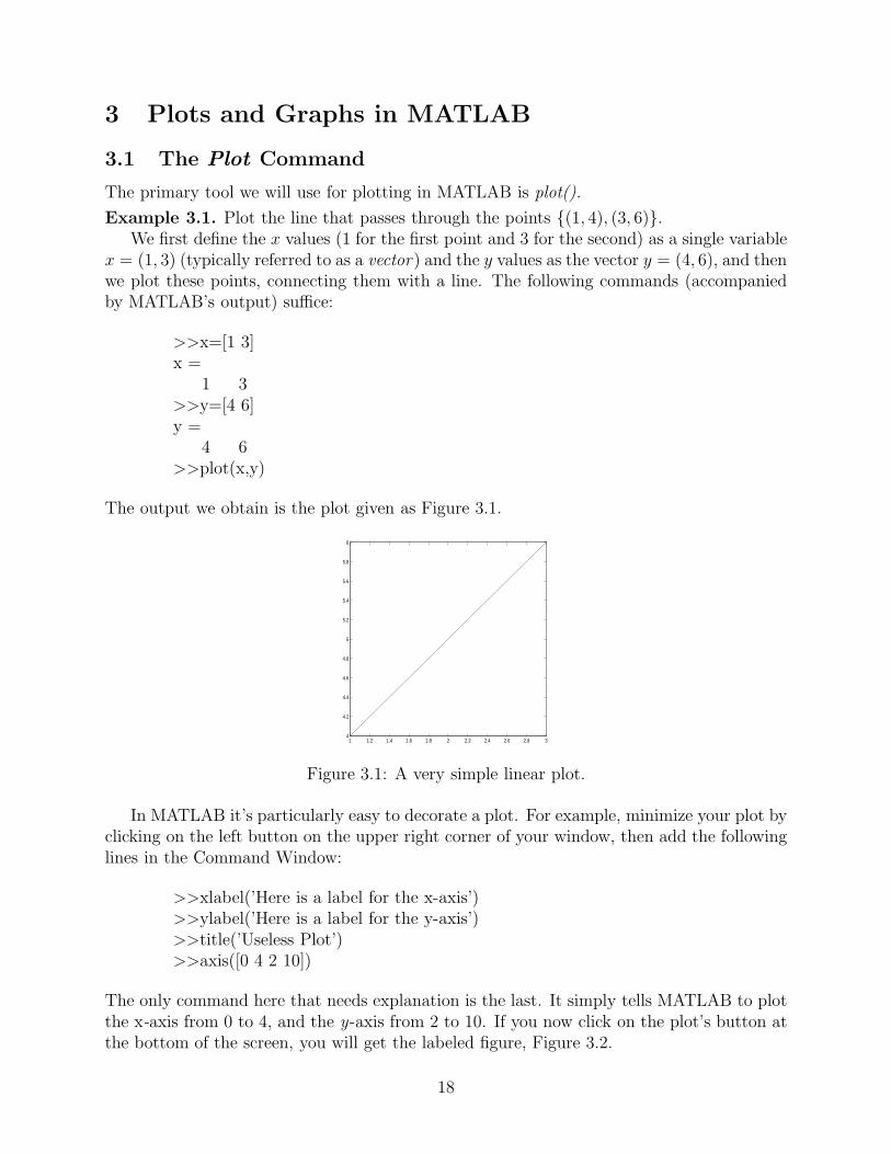
Example 3.1. Plot the line that passes through the points {(1, 4), (3, 6)}.We first define the x values (1 for the first point and 3 for the second) as a single variable

x = (1, 3) (typically referred to as a vector) and the y values as the vector y = (4, 6), and thenwe plot these points, connecting them with a line. The following commands (accompaniedby MATLAB’s output) suffice:

>>x=[1 3]x =

1 3>>y=[4 6]y =

4 6>>plot(x,y)

The output we obtain is the plot given as Figure 3.1.

1 1.2 1.4 1.6 1.8 2 2.2 2.4 2.6 2.8 34

4.2

4.4

4.6

4.8

5

5.2

5.4

5.6

5.8

6

Figure 3.1: A very simple linear plot.

In MATLAB it’s particularly easy to decorate a plot. For example, minimize your plot byclicking on the left button on the upper right corner of your window, then add the followinglines in the Command Window:

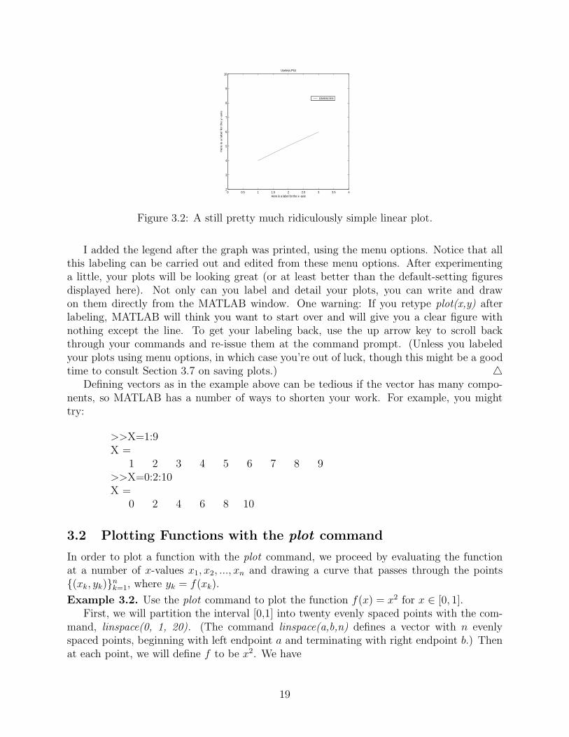
>>xlabel(’Here is a label for the x-axis’)>>ylabel(’Here is a label for the y-axis’)>>title(’Useless Plot’)>>axis([0 4 2 10])

The only command here that needs explanation is the last. It simply tells MATLAB to plotthe x-axis from 0 to 4, and the y-axis from 2 to 10. If you now click on the plot’s button atthe bottom of the screen, you will get the labeled figure, Figure 3.2.

18

0 0.5 1 1.5 2 2.5 3 3.5 42

3

4

5

6

7

8

9

10

Here is a label for the x−axis

He

re is a

la

be

l fo

r th

e y

−a

xis

Useless Plot

Useless line

Figure 3.2: A still pretty much ridiculously simple linear plot.

I added the legend after the graph was printed, using the menu options. Notice that allthis labeling can be carried out and edited from these menu options. After experimentinga little, your plots will be looking great (or at least better than the default-setting figuresdisplayed here). Not only can you label and detail your plots, you can write and drawon them directly from the MATLAB window. One warning: If you retype plot(x,y) afterlabeling, MATLAB will think you want to start over and will give you a clear figure withnothing except the line. To get your labeling back, use the up arrow key to scroll backthrough your commands and re-issue them at the command prompt. (Unless you labeledyour plots using menu options, in which case you’re out of luck, though this might be a goodtime to consult Section 3.7 on saving plots.) △

Defining vectors as in the example above can be tedious if the vector has many compo-nents, so MATLAB has a number of ways to shorten your work. For example, you mighttry:

>>X=1:9X =

1 2 3 4 5 6 7 8 9>>X=0:2:10X =

0 2 4 6 8 10

3.2 Plotting Functions with the plot command

In order to plot a function with the plot command, we proceed by evaluating the functionat a number of x-values x1, x2, ..., xn and drawing a curve that passes through the points{(xk, yk)}n

k=1, where yk = f(xk).

Example 3.2. Use the plot command to plot the function f(x) = x2 for x ∈ [0, 1].First, we will partition the interval [0,1] into twenty evenly spaced points with the com-

mand, linspace(0, 1, 20). (The command linspace(a,b,n) defines a vector with n evenlyspaced points, beginning with left endpoint a and terminating with right endpoint b.) Thenat each point, we will define f to be x2. We have

19

>>x=linspace(0,1,20)x =

Columns 1 through 80 0.0526 0.1053 0.1579 0.2105 0.2632 0.3158 0.3684

Columns 9 through 160.4211 0.4737 0.5263 0.5789 0.6316 0.6842 0.7368 0.7895

Columns 17 through 200.8421 0.8947 0.9474 1.0000

>>f=x.ˆ2f =

Columns 1 through 80 0.0028 0.0111 0.0249 0.0443 0.0693 0.0997 0.1357

Columns 9 through 160.1773 0.2244 0.2770 0.3352 0.3989 0.4681 0.5429 0.6233

Columns 17 through 200.7091 0.8006 0.8975 1.0000

>>plot(x,f)

Only three commands have been typed; MATLAB has done the rest. One thing you shouldpay close attention to is the line f=x.ˆ2, where we have used the array operation .ˆ. Thisoperation .ˆ signifies that the vector x is not to be squared (it’s not entirely clear at thispoint what we might even mean by the square of a vector), but rather that each componentof x is to be squared and the result is to be defined as a component of f , another vector.Similar commands are .* and ./. These are referred to as array operations, and you will needto become comfortable with their use. △Example 3.3. In our section on symbolic algebra, we encountered the logistic populationmodel, which relates the number of individuals in a population N with the rate of growthof the population R through the relationship

R(N) = aN(1 − N

K) = − a

KN2 + aN.

Taking a = 1 and K = 10, we have

R(N) = −.1N2 + N.

In order to plot this for populations between 0 and 20, we use the following MATLAB code,which creates Figure 3.3.

>>N=linspace(0,20,1000);>>R=-.1*N.ˆ2+N;>>plot(N,R)

Observe that the rate of growth is positive until the population achieves its “carrying capac-ity” of K = 10 and is negative for all populations beyond this. In this way, if the populationis initially below its carrying capacity, then it will increase toward its carrying capacity, butwill never exceed it. If the population is initially above the carrying capacity, it will decreasetoward the carrying capacity. The carrying capacity is interpreted as the maximum numberof individuals the environment can sustain. △

20

0 2 4 6 8 10 12 14 16 18 20−20

−15

−10

−5

0

5

Figure 3.3: Growth rate for the logistic model.

3.3 Parametric Curves

In certain cases the relationship between x and y can be described in terms of a thirdvariable, say t. In such cases, t is a parameter, and we refer to a plot of the points (x, y) asa parametric curve.

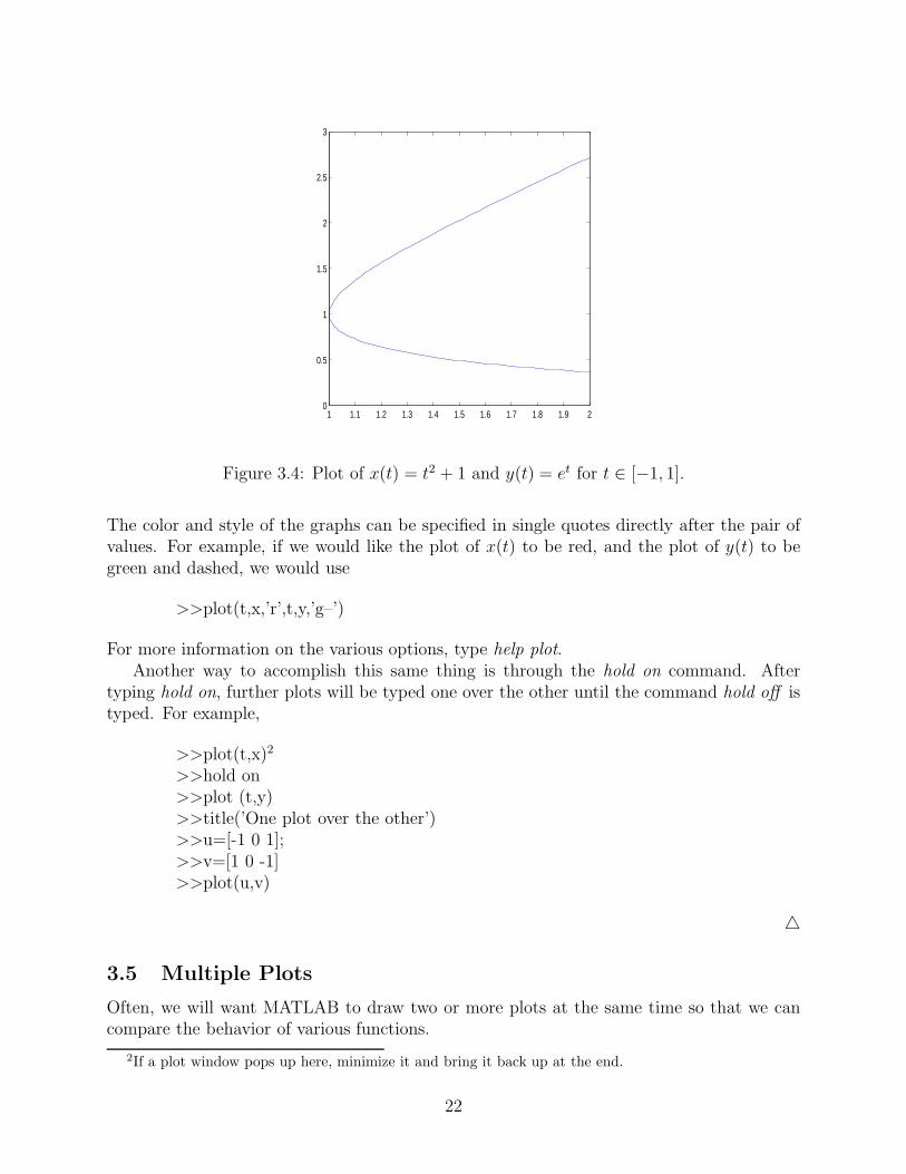
Example 3.4. Plot a curve in the x-y plane corresponding with x(t) = t2 +1 and y(t) = et,for t ∈ [−1, 1]. One way to accomplish this is through solving for t in terms of x andsubstituing your result into y(t) to get y as a function of x. Here, rather, we will simply getvalues of x and y at the same values of t. Using semicolons to suppress MATLAB’s output,we use the following script, which creates Figure 3.4.

>>t=linspace(-1,1,100);>>x=t.ˆ2 + 1;>>y=exp(t);>>plot(x,y)

△

3.4 Juxtaposing One Plot On Top of Another

Example 3.5. For the functions x(t) = t2 + 1 and y(t) = et, plot x(t) and y(t) on the samefigure, both versus t.

The easiest way to accomplish this is with the single command

>>plot(t,x,t,y);

21

1 1.1 1.2 1.3 1.4 1.5 1.6 1.7 1.8 1.9 20

0.5

1

1.5

2

2.5

3

Figure 3.4: Plot of x(t) = t2 + 1 and y(t) = et for t ∈ [−1, 1].

The color and style of the graphs can be specified in single quotes directly after the pair ofvalues. For example, if we would like the plot of x(t) to be red, and the plot of y(t) to begreen and dashed, we would use

>>plot(t,x,’r’,t,y,’g–’)

For more information on the various options, type help plot.Another way to accomplish this same thing is through the hold on command. After

typing hold on, further plots will be typed one over the other until the command hold off istyped. For example,

>>plot(t,x)2

>>hold on>>plot (t,y)>>title(’One plot over the other’)>>u=[-1 0 1];>>v=[1 0 -1]>>plot(u,v)

△

3.5 Multiple Plots

Often, we will want MATLAB to draw two or more plots at the same time so that we cancompare the behavior of various functions.

2If a plot window pops up here, minimize it and bring it back up at the end.

22

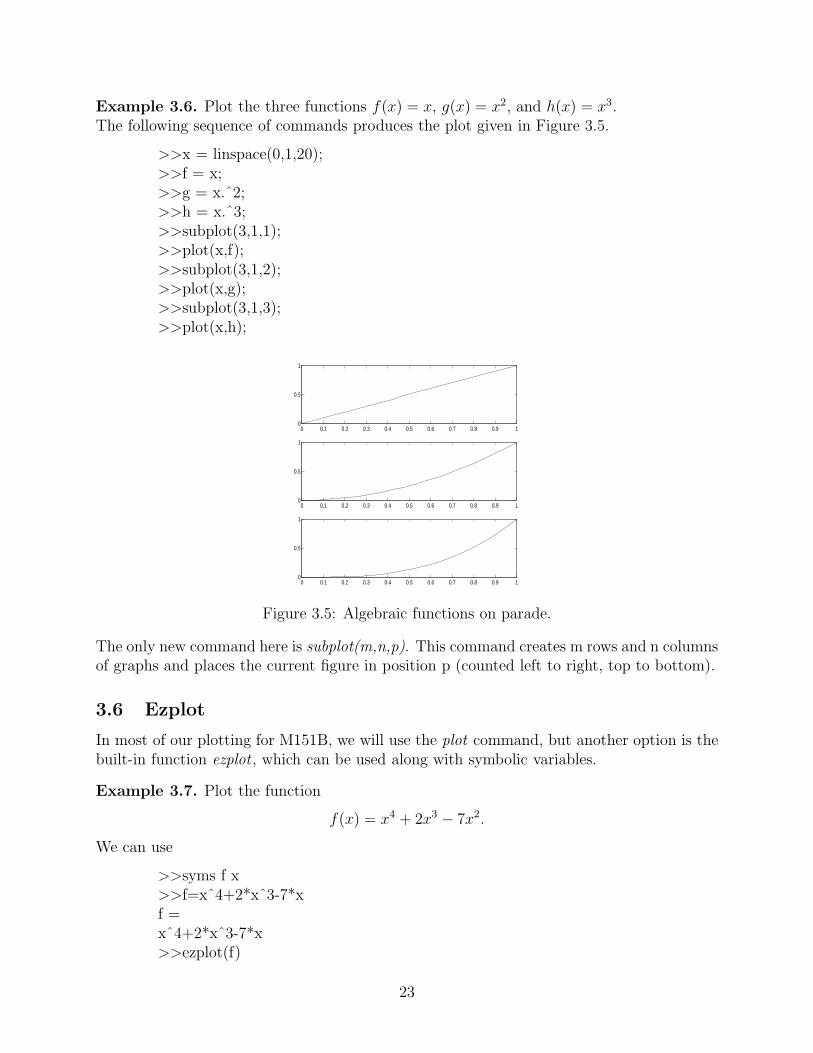
Example 3.6. Plot the three functions f(x) = x, g(x) = x2, and h(x) = x3.The following sequence of commands produces the plot given in Figure 3.5.

>>x = linspace(0,1,20);>>f = x;>>g = x.ˆ2;>>h = x.ˆ3;>>subplot(3,1,1);>>plot(x,f);>>subplot(3,1,2);>>plot(x,g);>>subplot(3,1,3);>>plot(x,h);

0 0.1 0.2 0.3 0.4 0.5 0.6 0.7 0.8 0.9 10

0.5

1

0 0.1 0.2 0.3 0.4 0.5 0.6 0.7 0.8 0.9 10

0.5

1

0 0.1 0.2 0.3 0.4 0.5 0.6 0.7 0.8 0.9 10

0.5

1

Figure 3.5: Algebraic functions on parade.

The only new command here is subplot(m,n,p). This command creates m rows and n columnsof graphs and places the current figure in position p (counted left to right, top to bottom).

3.6 Ezplot

In most of our plotting for M151B, we will use the plot command, but another option is thebuilt-in function ezplot , which can be used along with symbolic variables.

Example 3.7. Plot the function

f(x) = x4 + 2x3 − 7x2.

We can use

>>syms f x>>f=xˆ4+2*xˆ3-7*xf =xˆ4+2*xˆ3-7*x>>ezplot(f)

23

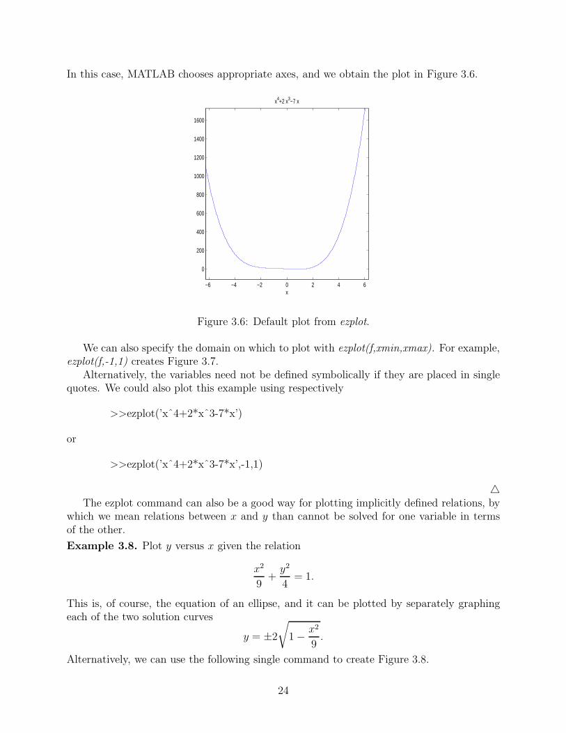
In this case, MATLAB chooses appropriate axes, and we obtain the plot in Figure 3.6.

−6 −4 −2 0 2 4 6

0

200

400

600

800

1000

1200

1400

1600

x

x4+2 x3−7 x

Figure 3.6: Default plot from ezplot.

We can also specify the domain on which to plot with ezplot(f,xmin,xmax). For example,ezplot(f,-1,1) creates Figure 3.7.

Alternatively, the variables need not be defined symbolically if they are placed in singlequotes. We could also plot this example using respectively

>>ezplot(’xˆ4+2*xˆ3-7*x’)

or

>>ezplot(’xˆ4+2*xˆ3-7*x’,-1,1)

△The ezplot command can also be a good way for plotting implicitly defined relations, by

which we mean relations between x and y than cannot be solved for one variable in termsof the other.

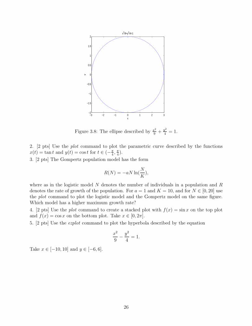
Example 3.8. Plot y versus x given the relation

x2

9+

y2

4= 1.

This is, of course, the equation of an ellipse, and it can be plotted by separately graphingeach of the two solution curves

y = ±2

√

1 − x2

9.

Alternatively, we can use the following single command to create Figure 3.8.

24

−1 −0.8 −0.6 −0.4 −0.2 0 0.2 0.4 0.6 0.8 1

−4

−2

0

2

4

6

x

x4+2 x3−7 x

Figure 3.7: Domain specified plot with ezplot.

>>ezplot(’xˆ2/9+yˆ2/4=1’,[-3,3],[-2,2])

Here, observe that the first interval specifies the values of x and the second specifies thevalues for y. △

Finally, we can use ezplot to plot parametrically defined relations.

Example 3.9. Use ezplot to plot y versus x, given x(t) = t2+1 and y(t) = et, for t ∈ [−1, 1].We can accomplish this with the single command

>>ezplot(’tˆ2+1’,’exp(t)’,[-1,1])

△

3.7 Saving Plots as Encapsulated Postscript Files

In order to print a plot, first save it as an encapsulated postscript file. From the options inyour graphics box, choose File, Save As, and change Save as type to EPS file. Finally,click on the Save button. The plot can now be printed using the xprint command.

Once saved as an encapsulated postscript file, the plot cannot be edited, so it should alsobe saved as a MATLAB figure. This is accomplished by choosing File, Save As, and savingthe plot as a .fig file (which is MATLAB’s default).

3.8 Assignments

For each of these assignments, turn in the indicated plot.

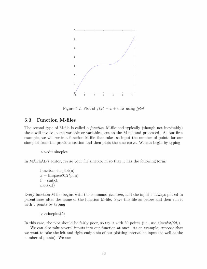
1. [2 pts] Use the plot command to plot the function f(x) = x + sin x for x ∈ [0, 2π]. Labelyour x and y axes and add a title to your plot.

25

−3 −2 −1 0 1 2 3−2

−1.5

−1

−0.5

0

0.5

1

1.5

2

x

y

x2/9+y2/4=1

Figure 3.8: The ellipse described by x2

9+ y2

4= 1.

2. [2 pts] Use the plot command to plot the parametric curve described by the functionsx(t) = tan t and y(t) = cos t for t ∈ (−π

4, π

4).

3. [2 pts] The Gompertz population model has the form

R(N) = −aN ln(N

K),

where as in the logistic model N denotes the number of individuals in a population and Rdenotes the rate of growth of the population. For a = 1 and K = 10, and for N ∈ [0, 20] usethe plot command to plot the logistic model and the Gompertz model on the same figure.Which model has a higher maximum growth rate?

4. [2 pts] Use the plot command to create a stacked plot with f(x) = sin x on the top plotand f(x) = cos x on the bottom plot. Take x ∈ [0, 2π].

5. [2 pts] Use the ezplot command to plot the hyperbola described by the equation

x2

9− y2

4= 1.

Take x ∈ [−10, 10] and y ∈ [−6, 6].

26

4 Semilog and Double-log Plots

In many applications, the values of data points can range significantly, and it can becomeconvenient to work with log10 values of the original data. In such cases, we often work withsemilog or double-log (or log-log) plots.

4.1 Semilog Plots

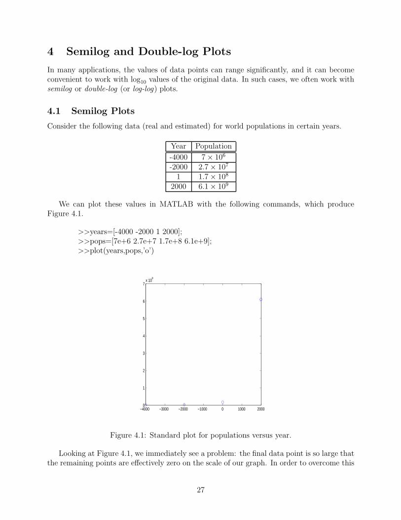
Consider the following data (real and estimated) for world populations in certain years.

Year Population

-4000 7 × 106

-2000 2.7 × 107

1 1.7 × 108

2000 6.1 × 109

We can plot these values in MATLAB with the following commands, which produceFigure 4.1.

>>years=[-4000 -2000 1 2000];>>pops=[7e+6 2.7e+7 1.7e+8 6.1e+9];>>plot(years,pops,’o’)

−4000 −3000 −2000 −1000 0 1000 20000

1

2

3

4

5

6

7x 10

9

Figure 4.1: Standard plot for populations versus year.

Looking at Figure 4.1, we immediately see a problem: the final data point is so large thatthe remaining points are effectively zero on the scale of our graph. In order to overcome this

27

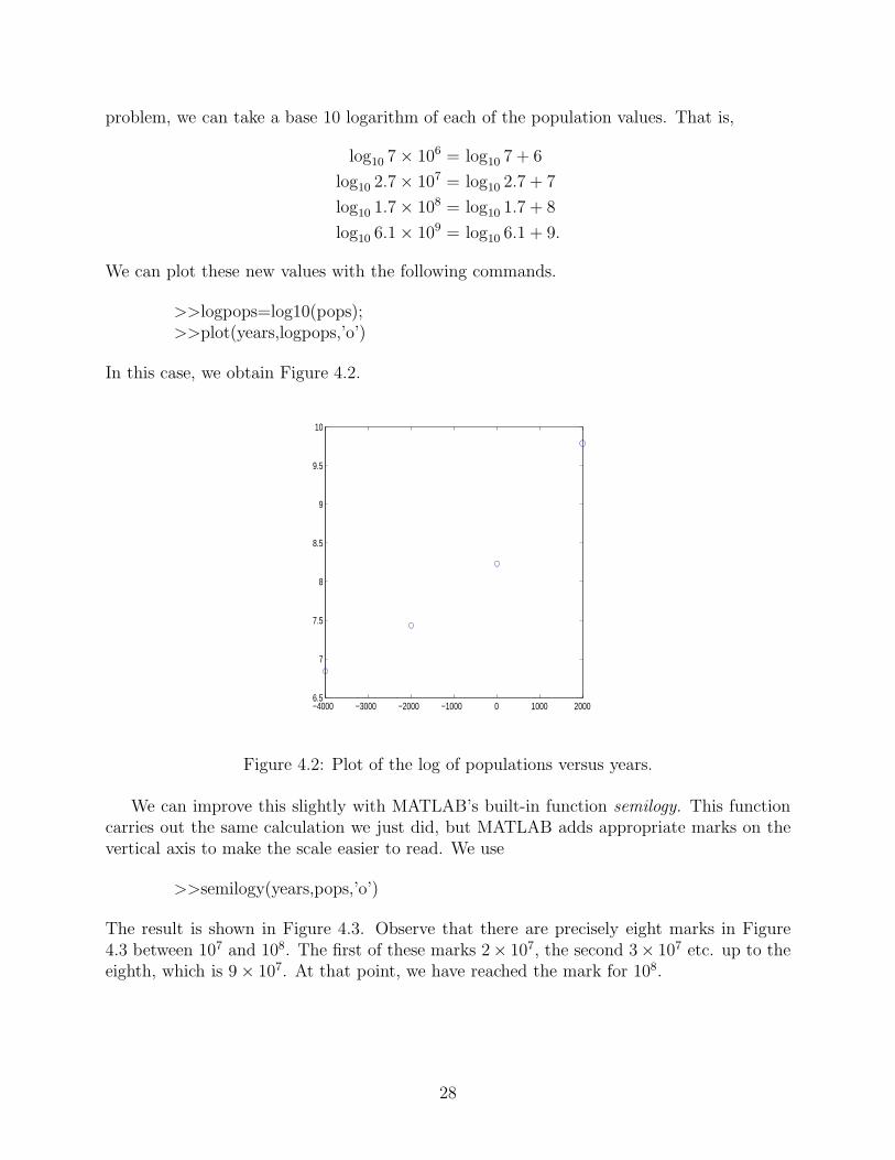
problem, we can take a base 10 logarithm of each of the population values. That is,

log10 7 × 106 = log10 7 + 6

log10 2.7 × 107 = log10 2.7 + 7

log10 1.7 × 108 = log10 1.7 + 8

log10 6.1 × 109 = log10 6.1 + 9.

We can plot these new values with the following commands.

>>logpops=log10(pops);>>plot(years,logpops,’o’)

In this case, we obtain Figure 4.2.

−4000 −3000 −2000 −1000 0 1000 20006.5

7

7.5

8

8.5

9

9.5

10

Figure 4.2: Plot of the log of populations versus years.

We can improve this slightly with MATLAB’s built-in function semilogy. This functioncarries out the same calculation we just did, but MATLAB adds appropriate marks on thevertical axis to make the scale easier to read. We use

>>semilogy(years,pops,’o’)

The result is shown in Figure 4.3. Observe that there are precisely eight marks in Figure4.3 between 107 and 108. The first of these marks 2× 107, the second 3× 107 etc. up to theeighth, which is 9 × 107. At that point, we have reached the mark for 108.

28

−4000 −3000 −2000 −1000 0 1000 200010

6

107

108

109

1010

Figure 4.3: Semilog plot of world population data.

4.1.1 Deriving Functional Relations from a Semilog Plot

Having plotted our population data, suppose we would like to find a relationship of the form

N = f(x),

where N denotes the number of individuals in the population during year x. We proceed byobserving that the four points in Figure 4.3 all lie fairly close to the same straight line. InSection ??, we will discuss how calculus can be used to find the exact form for such a line,but for now we simply allow MATLAB to carry out the computation. From the graphicswindow for Figure 4.2 (the figure created prior to the use of semilogy), choose Tools, BasicFitting. From the Basic Fitting menu, choose a Linear fit and check the box next toShow Equations. This produces Figure 4.4.

This line suggests that the relationship between N and x is

log10 N = .00048x + 8.6.

(Recall that we obtained this figure by taking log10 of our data.) Taking each side of thislast expression as an exponent for the base 10, we find

10log10 N = 10.00048x+8.6 = 10.00048x108.6.

We conclude with the functional relation

N(x) = 10.00048x108.6,

which is the form we were looking for.Finally, we note that MATLAB’s built-in function semilogx plots the x-axis on a loga-

rithmic scaling while leaving the y-axis in its original form.

29

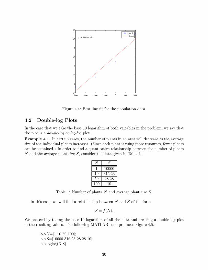
−4000 −3000 −2000 −1000 0 1000 20006.5

7

7.5

8

8.5

9

9.5

10

y = 0.00048*x + 8.6

data 1 linear

Figure 4.4: Best line fit for the population data.

4.2 Double-log Plots

In the case that we take the base 10 logarithm of both variables in the problem, we say thatthe plot is a double-log or log-log plot.

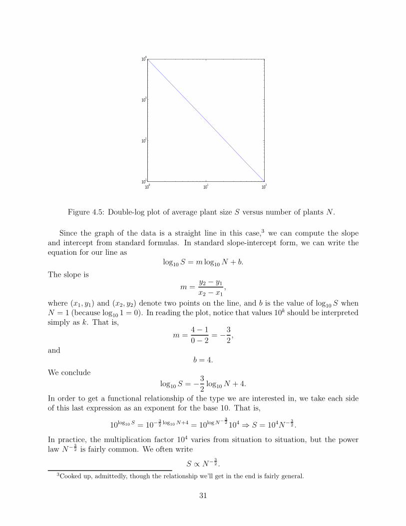
Example 4.1. In certain cases, the number of plants in an area will decrease as the averagesize of the individual plants increases. (Since each plant is using more resources, fewer plantscan be sustained.) In order to find a quantitative relationship between the number of plantsN and the average plant size S, consider the data given in Table 1.

N S

1 1000010 316.2350 28.28100 10

Table 1: Number of plants N and average plant size S.

In this case, we will find a relationship between N and S of the form

S = f(N).

We proceed by taking the base 10 logarithm of all the data and creating a double-log plotof the resulting values. The following MATLAB code produces Figure 4.5.

>>N=[1 10 50 100];>>S=[10000 316.23 28.28 10];>>loglog(N,S)

30

100

101

102

101

102

103

104

Figure 4.5: Double-log plot of average plant size S versus number of plants N .

Since the graph of the data is a straight line in this case,3 we can compute the slopeand intercept from standard formulas. In standard slope-intercept form, we can write theequation for our line as

log10 S = m log10 N + b.

The slope is

m =y2 − y1

x2 − x1

,

where (x1, y1) and (x2, y2) denote two points on the line, and b is the value of log10 S whenN = 1 (because log10 1 = 0). In reading the plot, notice that values 10k should be interpretedsimply as k. That is,

m =4 − 1

0 − 2= −3

2,

andb = 4.

We conclude

log10 S = −3

2log10 N + 4.

In order to get a functional relationship of the type we are interested in, we take each sideof this last expression as an exponent for the base 10. That is,

10log10 S = 10−3

2log10 N+4 = 10log N−

32 104 ⇒ S = 104N− 3

2 .

In practice, the multiplication factor 104 varies from situation to situation, but the powerlaw N− 3

2 is fairly common. We often write

S ∝ N− 3

2 .3Cooked up, admittedly, though the relationship we’ll get in the end is fairly general.

31

△

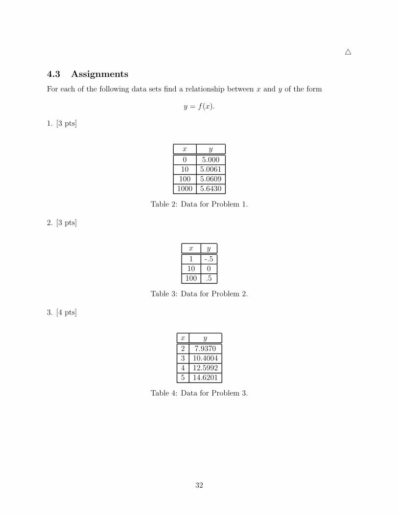
4.3 Assignments

For each of the following data sets find a relationship between x and y of the form

y = f(x).

1. [3 pts]

x y

0 5.00010 5.0061100 5.06091000 5.6430

Table 2: Data for Problem 1.

2. [3 pts]

x y

1 -.510 0100 .5


3. [4 pts]

x y

2 7.93703 10.40044 12.59925 14.6201


32

5 Inline Functions and M-Files

Functions can be defined in MATLAB either in line (that is, at the command prompt) or asM-files (separate text files).

5.1 Inline Functions

Example 5.1. Define the function f(x) = ex in MATLAB and compute f(1).We can accomplish this, as follows, with MATLAB’s built-in inline function.

>>f=inline(’exp(x)’)>>f(1)ans =2.7183

Observe, in particular, the difference between f(1) when f is a function and f(1) when f isa vector: if f is a vector, then f(1) is the first component of f , not the function f evaluatedat 1. △

In a similar manner, we can define a function of several variables.

Example 5.2. Define the function f(x, y) = x2 + y2 in MATLAB and compute f(1, 2).In this case, we use

>>f=inline(’xˆ2 + yˆ2’,’x’,’y’)f =

Inline function:f(x,y) = xˆ2 + yˆ2

>>f(1,2)ans =

5

Notice that in the case of multiple variables we specify the order in which the variables willappear as arguments of f . Compare the previous code with the following, in which MATLABexpects y as the first input of f and x as the second.4

f=inline(’xˆ2+yˆ2’,’y’,’x’)f =Inline function:f(y,x) = xˆ2+yˆ2

△In many cases we would like to define functions that use MATLAB’s array operations .ˆ,

.*, and ./. This can be accomplished either by typing the array operations in by hand or byusing the vectorize command.

Example 5.3. Define the function f(x) = x2 in MATLAB in such a way that MATLABcan take vector input and return vector output. Compute f(x) if x is the vector x = [1, 2].

We use4Granted, in this example order doesn’t matter.

33

>>f=inline(vectorize(’xˆ2’))f =

Inline function:f1(x) = x.ˆ2

>>x=[1 2]x =

1 2>>f(x)ans =

1 4

△Finally, in some cases it is convenient to define an inline function when the variables are

symbolic. Since the inline function expects a string, or character, as input, we first convertthe symbolic expression into a string expression.

Example 5.4. Compute the inverse of the function

f(x) =1

x + 1, x > −1,

and define the result as a MATLAB inline function. Compute f−1(5).We use

>>finv=solve(’1/(x+1)=y’)finv =-(y-1)/y>>finv=inline(char(finv))finv =Inline function:finv(y) = -(y-1)/y>>finv(5)ans =-0.8000

Observe that the variable finv is originally defined symbolically even though the expressionMATLAB solves is given as a string. The char command converts finv into a string, whichis appropriate as input for inline. △

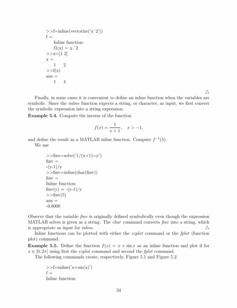
Inline functions can be plotted with either the ezplot command or the fplot (functionplot) command.

Example 5.5. Define the function f(x) = x + sin x as an inline function and plot if forx ∈ [0, 2π] using first the ezplot command and second the fplot command.

The following commands create, respectively, Figure 5.1 and Figure 5.2.

>>f=inline(’x+sin(x)’)f =Inline function:

34

f(x) = x+sin(x)>>ezplot(f,[0 2*pi])>>fplot(f,[0 2*pi])

△

0 1 2 3 4 5 6

0

1

2

3

4

5

6

x

x+sin(x)

Figure 5.1: Plot of f(x) = x + sin x using ezplot.

5.2 Script M-Files

The heart of MATLAB lies in its use of M-files. We will begin with a script M-file, which issimply a text file that contains a list of valid MATLAB commands. To create an M-file, clickon File at the upper left corner of your MATLAB window, then select New, followed by M-file. A window will appear in the upper left corner of your screen with MATLAB’s defaulteditor. (You are free to use an editor of your own choice, but for the brief demonstrationhere, let’s stick with MATLAB’s.) In this window, type the following lines:

x = linspace(0,2*pi,50);f = sin(x);plot(x,f)

Save this file by choosing File, Save As from the main menu. In this case, save the file assineplot.m, and then close or minimize your editor window. Back at the command line, typesineplot at the prompt, and MATLAB will plot the sine function on the domain [0, 2π]. Ithas simply gone through your file line by line and executed each command as it came to it.

35

0 1 2 3 4 5 60

1

2

3

4

5

6

7

Figure 5.2: Plot of f(x) = x + sin x using fplot

5.3 Function M-files

The second type of M-file is called a function M-file and typically (though not inevitably)these will involve some variable or variables sent to the M-file and processed. As our firstexample, we will write a function M-file that takes as input the number of points for oursine plot from the previous section and then plots the sine curve. We can begin by typing

>>edit sineplot

In MATLAB’s editor, revise your file sineplot.m so that it has the following form:

function sineplot(n)x = linspace(0,2*pi,n);f = sin(x);plot(x,f)

Every function M-file begins with the command function, and the input is always placed inparentheses after the name of the function M-file. Save this file as before and then run itwith 5 points by typing

>>sineplot(5)

In this case, the plot should be fairly poor, so try it with 50 points (i.e., use sineplot(50)).We can also take several inputs into our function at once. As an example, suppose that

we want to take the left and right endpoints of our plotting interval as input (as well as thenumber of points). We use

36

function sineplot(a,b,n)x = linspace(a,b,n);f = sin(x);plot(x,f)

Here, observe that order is important, so when you call the function you will need to putyour inputs in the same order as they are read by the M-file. For example, to again plot sineon [0, 2π], we use

>>sineplot(0,2*pi,50).

MATLAB can also take multiple inputs as a vector. Suppose the three values 0, 2π, and 50are stored in the vector v. That is, in MATLAB you have typed

>>v=[0,2*pi,50];

In this case, we write a function M-file that takes v as input and appropriately places itscomponents.

function sineplot(v)x = linspace(v(1),v(2),v(3));f = sin(x);plot(x,f)

5.4 Functions that Return Values

In the function M-files we have considered so far, the files have taken data as input, but theyhave not returned values. In order to see how MATLAB returns values, suppose we want tocompute the maximum value of sin(x) on the interval over which we are plotting it. Changesineplot.m as follows:

function maxvalue = sineplot(v)x = linspace(v(1),v(2),v(3));f = sin(x);maxvalue = max(f);plot(x,f)

In this new version, we have made two important changes. First, we have added maxvalue =to our first line, specifying that the value we want MATLAB to return is the one we computeas maxvalue. Second, we have added a line to the code that computes the maximum of fand assigns its value to the variable maxvalue. (The MATLAB function max takes vectorinput and returns the largest component.) When running an M-file that returns data fromthe command window, you will typically want to assign the returned value a designation.Here, you might use

>>m=sineplot(v)

37

The maximum of sin(x) on this interval will be recorded as the value of m.MATLAB can also return multiple values. Suppose we would like to return both the

maximum and the minimum of f in this example. We use

function [minvalue,maxvalue] = sineplot(v)x = linspace(v(1),v(2),v(3));f = sin(x);minvalue = min(f);maxvalue = max(f);plot(x,f)

In this case, at the command prompt, type

>>[m,n]=sineplot(v)

The value of m will now be the minimum of sin(x) on this interval, while n will be themaximum.

As our last example, we will write a function M-file that takes vector input and returnsvector output. In this case, the input will be as before, and we will record the minimum andmaximum of f in a vector. We have

function w = sineplot(v)x = linspace(v(1),v(2),v(3));f = sin(x);w = [min(f),max(f)];plot(x,f)

This function can be called with

>>b=sineplot(v)

where it is now understood that b is a vector with two components.

5.5 Debugging M-files

Since MATLAB views M-files as computer programs, it offers a handful of tools for debug-ging. First, from the M-file edit window, an M-file can be saved and run by clicking on theicon with the white sheet and downward-directed blue arrow (alternatively, choose Debug,Run or simply type F5). By setting your cursor on a line and clicking on the icon with thewhite sheet and the red dot, you can set a marker at which MATLAB’s execution will stop.A green arrow will appear, marking the point where MATLAB’s execution has paused. Atthis point, you can step through the rest of your M-file one line at a time by choosing theStep icon (alternatively Debug, Step or F6).

Unless you’re a phenomenal programmer, you will occasionally write a MATLAB program(M-file) that has no intention of stopping any time in the near future. You can always abortyour program by typing Control-c, though you must be in the MATLAB Command Windowfor MATLAB to pay any attention to this. If all else fails, Control-Alt-Backspace willend your session on a calclab account.

38

5.6 Assignments

For the logistic population model

R(N) = aN(1 − N

K),

the number of individuals in the population can be written as a function of time t (and theparameters of the model) as

N(t, a, K, N0) =N0K

N0 + (K − N0)e−at,

where N0 is the number of individuals at time 0.

1. [2.5 pts ]Define the function N(t, a, K, N0) as an inline function and compute the popu-lation for t = 10, a = .1, K = 100, and N0 = 5.

2. [2.5 pts] Write a script M-file that plots N as a function of t for the parameter valuesgiven in problem 1. Take t ∈ [0, 5].

3. [2.5 pts] Write a function M-file that takes the parameters a, K, and N0 as input andplots N as a function of t for t ∈ [0, 5]. Use your M-file to plot N for the values a = .2,K = 100, N0 = 150.

4. [2.5] Write a function M-file that takes the parameters a, K, and N0 as input and returnsthe value of the population at t = 5.

39

6 Function Limits in MATLAB

6.1 Symbolic Limits of Functions

MATLAB’s symbolic toolbox has a function limit that can symbolically compute limits. Thesyntax for computing the limit

limx→a

f(x) = L

islimit(f(x),x,a),

where x is a symbolic variable.

Example 6.1. Compute the limit

limx→0

sin x

x= 1.

In MATLAB,

>>syms x;>>limit(sin(x)/x,x,0)ans =1

△Example 6.2. Compute the limit

limx→∞

x4 + x2 − 3

3x4 − log x=

1

3,

In MATLAB,

>>limit((xˆ4 + xˆ2 - 3)/(3*xˆ4 - log(x)),x,Inf)ans =1/3

△For left and right limits, the option ’left’ or ’right’ can be added at the end of the function

statement.

Example 6.3. Compute the left and right limits

limx→0−

|x|x

= −1; limx→0+

|x|x

= +1.

In MATLAB,

40

>>syms x;>>limit(abs(x)/x,x,0,’left’)ans =-1>>limit(abs(x)/x,x,0,’right’)ans =1

△

6.2 Divergence by Oscillation

In class we have observed that in certain cases a limit can fail to exist because the graph ofthe function continues to oscillate as the independent variable approaches its limit. In thissubsection, we will consider an example of such a case.

Example 6.4. Consider the limit

limx→0

sin1

x.

In order to study this limit, we will plot the function sin 1x

for x near 0. We use

>>x=linspace(.03, .5, 1000);>>f=sin(1./x);>>plot(x,f)

We see in Figure 6.1 that as x goes toward 0, sin 1x

continues to oscillate between -1 and +1,with the period of oscillation becoming shorter and shorter. △

6.3 The Sandwich Theorem

In class, we considered the following Sandwich Theorem ( sometimes called the Squeeze The-orem):

Sandwich Theorem. If f(x) ≤ g(x) ≤ h(x) for all x in an open interval containing c(except possibly at c) and

limx→c

f(x) = limx→c

h(x) = L,

thenlimx→0

g(x) = L.

Example 6.5. Consider the limit

limx→0

x sin1

x.

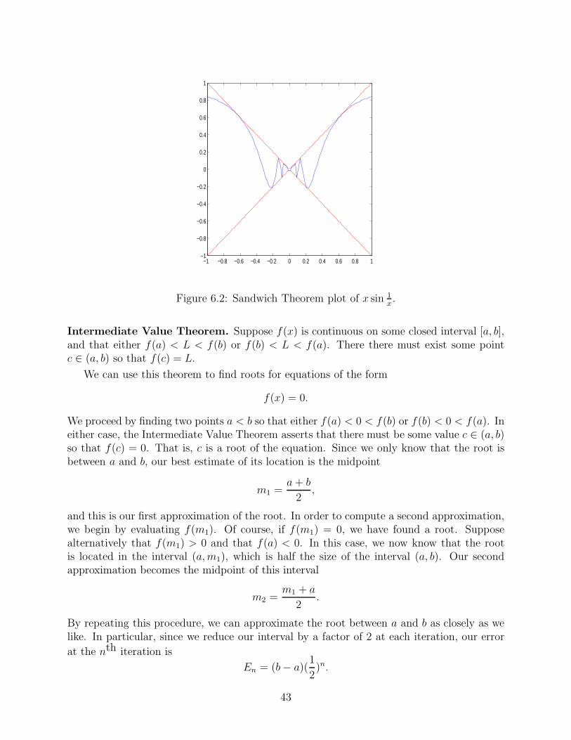
Our approach to this limit in class was to apply with Sandwich Theorem with theinequalities

−|x| ≤ x sin1

x≤ |x|.

In order to see how this looks graphically, let’s plot all three of these functions together ona MATLAB figure. We use the commands

41

0 0.1 0.2 0.3 0.4 0.5 0.6−1

−0.8

−0.6

−0.4

−0.2

0

0.2

0.4

0.6

0.8

1

Figure 6.1: Plot of sin 1x.

>>x=linspace(-1,1,100);>>f=-abs(x);>>g=x.*sin(1./x);>>h=abs(x);>>plot(x,f,’r’,x,g,x,h,’r’)

Here, the bounding functions f(x) and h(x) have been drawn in red with the option ’r’ (thiswon’t appear in the black and white figure in these notes). △

Example 6.6. We also use the Sandwich Theorem to establish the limit

limx→0

sin x

x= 1.

In order to see this limit graphically, we use the following MATLAB code.

>>x=linspace(-1, 1, 1000);>>f=sin(x)./x;>>plot(x,f)

This creates Figure 6.3, in which we see that for x either above or below 0, the limit isapproaching 1. △

6.4 The Bisection Method

In class, we used the Intermediate Value Theorem to develop the bisection method for findingroots of functions.

42

−1 −0.8 −0.6 −0.4 −0.2 0 0.2 0.4 0.6 0.8 1−1

−0.8

−0.6

−0.4

−0.2

0

0.2

0.4

0.6

0.8

1

Figure 6.2: Sandwich Theorem plot of x sin 1x.

Intermediate Value Theorem. Suppose f(x) is continuous on some closed interval [a, b],and that either f(a) < L < f(b) or f(b) < L < f(a). There there must exist some pointc ∈ (a, b) so that f(c) = L.

We can use this theorem to find roots for equations of the form

f(x) = 0.

We proceed by finding two points a < b so that either f(a) < 0 < f(b) or f(b) < 0 < f(a). Ineither case, the Intermediate Value Theorem asserts that there must be some value c ∈ (a, b)so that f(c) = 0. That is, c is a root of the equation. Since we only know that the root isbetween a and b, our best estimate of its location is the midpoint

m1 =a + b

2,

and this is our first approximation of the root. In order to compute a second approximation,we begin by evaluating f(m1). Of course, if f(m1) = 0, we have found a root. Supposealternatively that f(m1) > 0 and that f(a) < 0. In this case, we now know that the rootis located in the interval (a, m1), which is half the size of the interval (a, b). Our secondapproximation becomes the midpoint of this interval

m2 =m1 + a

2.

By repeating this procedure, we can approximate the root between a and b as closely as welike. In particular, since we reduce our interval by a factor of 2 at each iteration, our error

at the nth iteration is

En = (b − a)(1

2)n.

43

−1 −0.8 −0.6 −0.4 −0.2 0 0.2 0.4 0.6 0.8 10.84

0.86

0.88

0.9

0.92

0.94

0.96

0.98

1

1.02

Figure 6.3: Plot of sinxx

.

Example 6.7. (Problem 8 from Section 3.5 of our text.) Use the bisection method to finda solution of

cos x = x

that is accurate to two decimal places (i.e., that has an error smaller than .01).In this case, the function of interest is f(x) = cos x−x, and we begin with the endpoints

a = 0 and b = 1, for which f(0) = 1 and f(1) = −.4597. Our first estimate is

m1 =1

2.

In order to find an estimate within two decimal places, we require the number of iterationsn to be large enough so that

(1

2)n < .01.

That is, we insist that our error is less than 1/100, even though rounding errors could actuallymake our two-decimal approximation differ from the correct answer by 1/100. Solving thisinequality for n we find that n must be large enough so that

n >log10 .01

log10 .5= 6.6439.

In other words, we require 7 iterations. We will carry this out in MATLAB. For the first fewiterations, we can proceed explicitly

>>cos(1/2)-1/2ans =0.3776

44

>>m2=(1+1/2)/2m2 =0.7500>>cos(m2)-m2ans =-0.0183>>m3=(.75+.5)/2m3 =0.6250

Repeating this 7 times will get old fast, so let’s finish the calculation with an M-file, bisec-tion.m.5

function value = bisection(a,b,n)f=inline(’cos(x)-x’,’x’);fleft = f(a);fright = f(b);for k=1:nm(k) = (a+b)/2;fmid = f(m(k));if fmid*fleft > 0a = m(k);elseb = m(k);endendvalue = m;

In this M-file, we take left and right endpoints as input, as well as the number of iterationsn. At step k, our approximation is mk, which in MATLAB looks like m(k). The file returnsa vector containing the approximation at each iteration.

>>bisection(0,1,7)ans =0.5000 0.7500 0.6250 0.6875 0.7188 0.7344 0.7422

Here, the approximation at step 7 is m7 = .7422, which we compare with the exact solutionmexact = .7391 (to four decimal places). We see indeed that our approximation is good totwo decimal places (i.e., |m1 − mexact| = .0031 < .01). △

5This M-file, along with several others, is available on the course web site.

45

6.5 Experimenting with the Formal Definition of Limits

The formal definition of a (finite) limit is given as follows:

Definition. The statementlimx→c

f(x) = L

means that for any ǫ > 0 there exists some δ > 0 so that if 0 < |x−c| < δ then |f(x)−L| < ǫ.(Recall that we take |x − c| > 0, or equivalently x 6= c, because f(x) may not be defined atx = c.) That is, by taking x sufficiently close to its limiting value c, we can force f(x) to

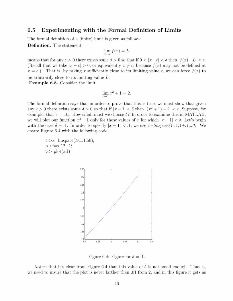
be arbitrarily close to its limiting value L.Example 6.8. Consider the limit

limx→1

x2 + 1 = 2.

The formal definition says that in order to prove that this is true, we must show that givenany ǫ > 0 there exists some δ > 0 so that if |x− 1| < δ then |(x2 + 1)− 2| < ǫ. Suppose, forexample, that ǫ = .01. How small must we choose δ? In order to examine this in MATLAB,we will plot our function x2 + 1 only for those values of x for which |x− 1| < δ. Let’s beginwith the case δ = .1. In order to specify |x − 1| < .1, we use x=linspace(1-.1,1+.1,50). Wecreate Figure 6.4 with the following code.

>>x=linspace(.9,1.1,50);>>f=x.ˆ2+1;>> plot(x,f)

0.9 0.95 1 1.05 1.1 1.151.8

1.85

1.9

1.95

2

2.05

2.1

2.15

2.2

2.25

Figure 6.4: Figure for δ = .1.

Notice that it’s clear from Figure 6.4 that this value of δ is not small enough. That is,we need to insure that the plot is never farther than .01 from 2, and in this figure it gets as

46

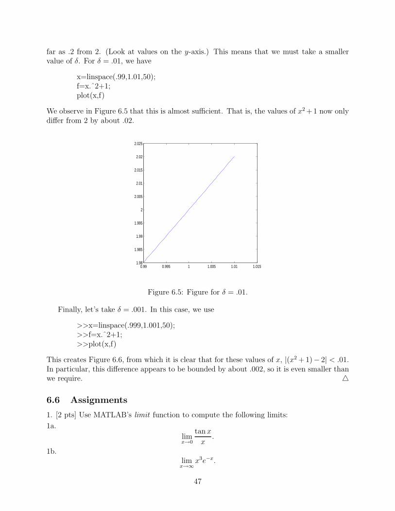
far as .2 from 2. (Look at values on the y-axis.) This means that we must take a smallervalue of δ. For δ = .01, we have

x=linspace(.99,1.01,50);f=x.ˆ2+1;plot(x,f)

We observe in Figure 6.5 that this is almost sufficient. That is, the values of x2 +1 now onlydiffer from 2 by about .02.

0.99 0.995 1 1.005 1.01 1.0151.98

1.985

1.99

1.995

2

2.005

2.01

2.015

2.02

2.025


Finally, let’s take δ = .001. In this case, we use

>>x=linspace(.999,1.001,50);>>f=x.ˆ2+1;>>plot(x,f)

This creates Figure 6.6, from which it is clear that for these values of x, |(x2 + 1)− 2| < .01.In particular, this difference appears to be bounded by about .002, so it is even smaller thanwe require. △

6.6 Assignments

1. [2 pts] Use MATLAB’s limit function to compute the following limits:

1a.

limx→0

tan x

x.

1b.lim

x→∞x3e−x.

47

0.999 0.9992 0.9994 0.9996 0.9998 1 1.0002 1.0004 1.0006 1.0008 1.0011.998

1.9985

1.999

1.9995

2

2.0005

2.001

2.0015

2.002

2.0025


1c.lim

x→1+e−

1

1−x .

2. [2 pts] The limit

limx→0+

sin x

x= 1

can be established by using the Squeeze Theorem and the inequality

cos x ≤ sin x

x≤ 1

cos x,

for x ∈ (0, π2). Depict this graphically by proceeding similarly as in Example 6.5.

3. [2 pts] Find the number of iterations n that will insure that the solution to

x = tan x,

for x ∈ (π8, 3π

8) is accurate to two decimal places.

4. [2 pts] Alter bisection.m so that the function f(x) is taken (in the form of an inlinefunction) as input in the function call statement. Use your new M-file to find the root for

f(x) = x − tanx

for x ∈ (π8, 3π

8). Your error should be smaller than .01.

5. [2 pts] The limit

limx→1

(1 − .5x−1)

x − 1= ln(2)

48

means that given any ǫ > 0 there exists some δ > 0 so that

0 < |x − 1| < δ ⇒ |(1 − .5x−1)

x − 1− ln(2)| < ǫ.

Proceeding as in Example 6.8 find an appropriate value for δ if ǫ = .01.

49

7 Symbolic Derivatives in MATLAB

Symbolic derivatives can be computed in MATLAB with the command diff().

Example 7.1. Use the diff() command to compute the derivative of x3.We can compute this three different ways. First, we can proceed directly:

>>syms x;>>diff(xˆ3)ans =3*xˆ2

Alternatively, we can first define f(x) = x3 as an inline function.

>>syms x;>>f=inline(’xˆ3’,’x’);>>diff(f(x))ans =3*xˆ2

Finally, we can use diff without first specifying x as a symbolic variable by using singlequotes in the argument of diff.

>>diff(’xˆ3’)ans =3*xˆ2

△Example 7.2. Compute the derivative of f(x) = ex sin x. In MATLAB,

>>syms x;>>diff(exp(x)*sin(x))ans =exp(x)*sin(x)+exp(x)*cos(x)

△

7.1 Computing Higher Order Derivatives in MATLAB

The derivative of a function f(x) is again a function f ′(x). If we now take a derivative off ′(x), we have

d

dxf ′(x) = f ′′(x),

which we refer to as the second derivative of f . Alternatively, we have the notation

f ′′(x) =d2f

dx2.

50

Similarly, the third derivative of f is defined as

f ′′′(x) =d

dxf ′′(x),

and can also be written as

f ′′′(x) =d3f

dx3.

Proceeding similarly, we can define the derivative of a function to any order. Eventually, the

prime notation becomes unwieldy, and so we often write the nth derivative as

f (n)(x) =dnf

dxn.

Example 7.3. For f(x) = x3, compute f ′′(x) in MATLAB.As with first order derivatives, there are three ways in which to do this in MATLAB.

First, we can simply use the diff command, and specify in the second entry that we want asecond order derivative.

>>syms x;>>diff(xˆ3,2)ans =6*x

Alternatively, we can first specify f(x) as an inline function.

>>syms x;>>f=inline(’xˆ3’,’x’)f =Inline function:f(x) = xˆ3>>diff(f(x),2)ans =6*x

Finally, we can again use the diff command with single quotes.

>>diff(’xˆ3’,2)ans =6*x

△Example 7.4. Compute the third x-derivative of the function

f(x) = sin(ax).

Again, we can proceed in one of three different ways, though now we must specify whichvariable we want MATLAB to differentiate with respect to. First, we use

51

>>syms a x;>>diff(sin(a*x),x,3)ans =-cos(a*x)*aˆ3

(In fact, MATLAB takes x as its independent variable by default, so the statement diff(sin(a*x),3)would also work here, but in general you can use any letter (or combination of letters) asan independent variable, so long as you specify it as such.) Alternatively, we can define aninline function as a function of both x and a, and then specify that we want to differentiatewith respect to x.

>>syms a x;>>f=inline(’sin(a*x)’,’a’,’x’)f =Inline function:f(a,x) = sin(a*x)>>diff(f(a,x),x,3)ans =-cos(a*x)*aˆ3

Finally, we can still use diff with single quotes bracing the argument. In this case, noticethat x must be placed in single quotes when being distinguished as the independent variable.

>>diff(’sin(a*x)’,’x’,3)ans =-cos(a*x)*aˆ3

△

7.2 Computing Derivatives as Limits

According to our definition, the derivative of a function f(x) can be computed as the limit

f ′(x) = limh→0

f(x + h) − f(x)

h.

Example 7.5. Use the definition of derivative to compute the derivative of f(x) = x2. InMATLAB,

>>syms x h;>>limit(((x+h)ˆ2-xˆ2)/h,h,0)ans =2*x

△Example 7.6. Use the definition of derivative to compute the derivatives of sin x and cos x.In MATLAB

52

>>syms x h;>>limit((sin(x+h)-sin(x))/h,h,0)ans =cos(x)>>limit((cos(x+h)-cos(x))/h,h,0)ans =-sin(x)

△

7.3 Dynamic and Geometric Interpretations of the Derivative

In studying calculus and its applications, it is extremely important to keep in mind boththe dynamic interpretation of the derivative as the rate of change of some process, and thegeometric interpretation of the derivative as the slope of the line that is tangent to the graphof the function at the specified point.

Example 7.7. The logistic population model relates the rate of growth R of a populationto the size of the population N by the relation

R(N) = aN(1 − N

K).

If N0 is the population at time 0, it is possible to show that

N(t) =K

1 + ( KN0

− 1)e−at.

In this example, we will investigate the behavior of this function for the values a = 1, N0 = 1,and K = 10, for which we have

N(t) =10

1 + 9e−t.

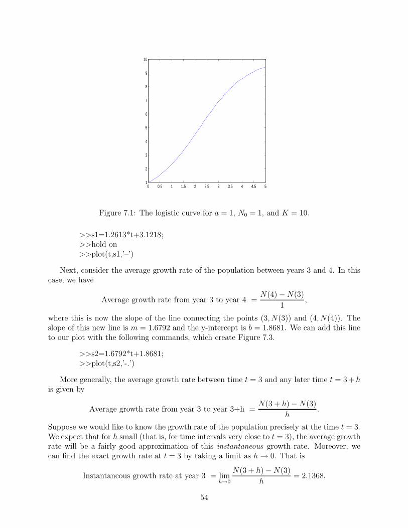
We can plot this function in MATLAB with the following commands, which create Figure7.1.

>>t=linspace(0,5,50);>>N=10./(1+9*exp(-t));>>plot(t,N)

The average growth rate of this population over any time period is given by

Average growth rate =Change in population

Length of time period.

For example, the average growth rate of this population from year 3 to year 5 is

Average growth rate from year 3 to year 5 =N(5) − N(3)

2.

In particular, notice that this value N(5)−N(3)2

is precisely the slope of the line connecting thepoints (3, N(3)) and (5, N(5)) (see Figure 7.2). This line is referred to as a secant line andhas slope m = 1.2613 and y-intercept b = 3.1218. It can be added to our figure with thefollowing commands, which create Figure 7.2.

53

0 0.5 1 1.5 2 2.5 3 3.5 4 4.5 51

2

3

4

5

6

7

8

9

10

Figure 7.1: The logistic curve for a = 1, N0 = 1, and K = 10.

>>s1=1.2613*t+3.1218;>>hold on>>plot(t,s1,’–’)

Next, consider the average growth rate of the population between years 3 and 4. In thiscase, we have

Average growth rate from year 3 to year 4 =N(4) − N(3)

1,

where this is now the slope of the line connecting the points (3, N(3)) and (4, N(4)). Theslope of this new line is m = 1.6792 and the y-intercept is b = 1.8681. We can add this lineto our plot with the following commands, which create Figure 7.3.

>>s2=1.6792*t+1.8681;>>plot(t,s2,’-.’)

More generally, the average growth rate between time t = 3 and any later time t = 3 + his given by

Average growth rate from year 3 to year 3+h =N(3 + h) − N(3)

h.

Suppose we would like to know the growth rate of the population precisely at the time t = 3.We expect that for h small (that is, for time intervals very close to t = 3), the average growthrate will be a fairly good approximation of this instantaneous growth rate. Moreover, wecan find the exact growth rate at t = 3 by taking a limit as h → 0. That is

Instantaneous growth rate at year 3 = limh→0

N(3 + h) − N(3)

h= 2.1368.

54

0 0.5 1 1.5 2 2.5 3 3.5 4 4.5 51

2

3

4

5

6

7

8

9

10

Figure 7.2: The logistic curve with a secant line.

This limit is the derivative of N(t) at the time t = 3 and corresponds precisely with the slopeof the line tangent to the curve of N(t) at the time t = 3. The y-interept associated withthis time is b = .4953, and so this line can be added to our plot with the following MATLABcommands, which create Figure 7.4. (The tangent line will appear in red on your figure.)

>>tangent=2.1368*t+.4953>>plot(t,tangent,’r’)

Generally speaking, we define a derivative of N(t) at any time t by the relation

dN

dt= lim

h→0

N(t + h) − N(t)

h.

The fundamental point regarding the geometry of the derivative is that it corresponds withthe slope of the line that is tangent to the curve at that point. △

7.4 Computing the Equation of the Tangent Line

It is clear from our geometric interpretation of derivative that for a differentiable functionf(x), if we want to compute the slope of the tangent line at some point value x = c, weneed only compute f ′(c). In the final example of this section, we will use this informationto compute the equation for the tangent line.

Example 7.8. Compute the equation of the line tangent to f(x) = cos x at the pointx0 = π

4.

We begin by computing the slope of this line, which is f ′(π4). In MATLAB,

55

0 0.5 1 1.5 2 2.5 3 3.5 4 4.5 51

2

3

4

5

6

7

8

9

10

11

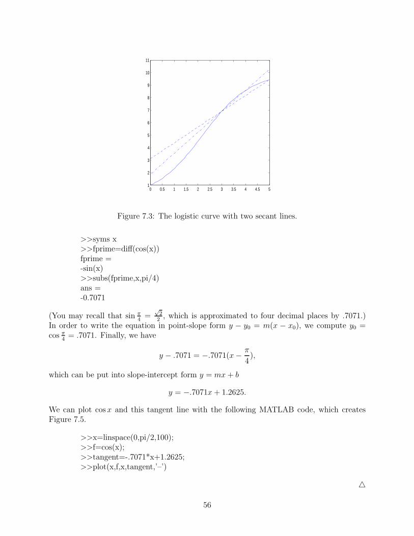
Figure 7.3: The logistic curve with two secant lines.

>>syms x>>fprime=diff(cos(x))fprime =-sin(x)>>subs(fprime,x,pi/4)ans =-0.7071

(You may recall that sin π4

=√

22

, which is approximated to four decimal places by .7071.)In order to write the equation in point-slope form y − y0 = m(x − x0), we compute y0 =cos π

4= .7071. Finally, we have

y − .7071 = −.7071(x − π

4),

which can be put into slope-intercept form y = mx + b

y = −.7071x + 1.2625.

We can plot cos x and this tangent line with the following MATLAB code, which createsFigure 7.5.

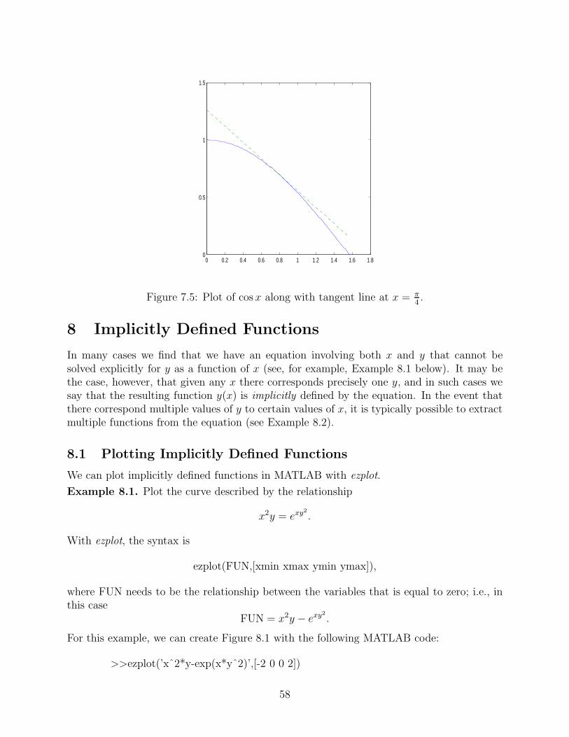
>>x=linspace(0,pi/2,100);>>f=cos(x);>>tangent=-.7071*x+1.2625;>>plot(x,f,x,tangent,’–’)

△

56

0 0.5 1 1.5 2 2.5 3 3.5 4 4.5 50

2

4

6

8

10

12

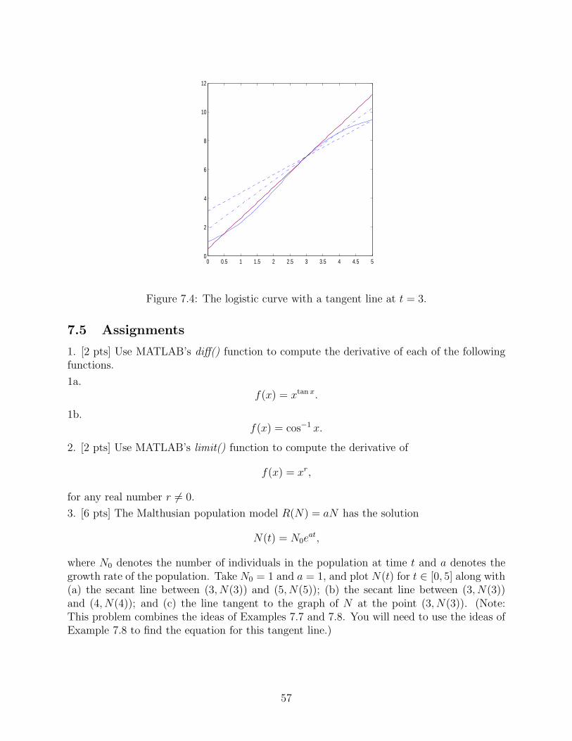
Figure 7.4: The logistic curve with a tangent line at t = 3.

7.5 Assignments

1. [2 pts] Use MATLAB’s diff() function to compute the derivative of each of the followingfunctions.

1a.f(x) = xtan x.

1b.f(x) = cos−1 x.

2. [2 pts] Use MATLAB’s limit() function to compute the derivative of

f(x) = xr,

for any real number r 6= 0.

3. [6 pts] The Malthusian population model R(N) = aN has the solution

N(t) = N0eat,

where N0 denotes the number of individuals in the population at time t and a denotes thegrowth rate of the population. Take N0 = 1 and a = 1, and plot N(t) for t ∈ [0, 5] along with(a) the secant line between (3, N(3)) and (5, N(5)); (b) the secant line between (3, N(3))and (4, N(4)); and (c) the line tangent to the graph of N at the point (3, N(3)). (Note:This problem combines the ideas of Examples 7.7 and 7.8. You will need to use the ideas ofExample 7.8 to find the equation for this tangent line.)

57

0 0.2 0.4 0.6 0.8 1 1.2 1.4 1.6 1.80

0.5

1

1.5

Figure 7.5: Plot of cosx along with tangent line at x = π4.

8 Implicitly Defined Functions

In many cases we find that we have an equation involving both x and y that cannot besolved explicitly for y as a function of x (see, for example, Example 8.1 below). It may bethe case, however, that given any x there corresponds precisely one y, and in such cases wesay that the resulting function y(x) is implicitly defined by the equation. In the event thatthere correspond multiple values of y to certain values of x, it is typically possible to extractmultiple functions from the equation (see Example 8.2).

8.1 Plotting Implicitly Defined Functions

We can plot implicitly defined functions in MATLAB with ezplot.

Example 8.1. Plot the curve described by the relationship

x2y = exy2

.

With ezplot, the syntax is

ezplot(FUN,[xmin xmax ymin ymax]),

where FUN needs to be the relationship between the variables that is equal to zero; i.e., inthis case

FUN = x2y − exy2

.

For this example, we can create Figure 8.1 with the following MATLAB code:

>>ezplot(’xˆ2*y-exp(x*yˆ2)’,[-2 0 0 2])

58

−2 −1.8 −1.6 −1.4 −1.2 −1 −0.8 −0.6 −0.4 −0.2 00

0.2

0.4

0.6

0.8

1

1.2

1.4

1.6

1.8

2

x

y

x2 y−exp(x y2) = 0

Figure 8.1: Plot of the relationship x2y = exy2

.

△Example 8.2. Write down the two functions y1(x) and y2(x) associated with the equation

x2 + y2 = 1.

In this case, we can solve for y to find

y(x) = ±√

1 − x2,

which is not a function since there correspond two values of y to each value of x. In thiscase, we have two functions

y1(x) = −√

1 − x2

y2(x) =√

1 − x2.

△

8.2 Tangent Lines for Implicitly Defined Relations

In order to compute the tangent line at a point for an implicitly defined relation, we requirea method for computing dy

dxthat does not require an explicit formula for y as a function of

x. We accomplish this with implicit differentiation.

Example 8.3. Plot the line tangent to the curve described in Example 8.1 at the pointx = −1. First, we need a value of y associated with x = −1, and we observe that from ourrelation we have

y = e−y2

.

Though we cannot solve this exactly, we can solve it in MATLAB with the following code.

59

>>y=solve(’y-exp(-yˆ2)’,’y’)y =exp(-1/2*lambertw(2))>>eval(y)ans =0.6529

Our point is (−1, .6529). In order to find the slope of the tangent line, we compute dy

dxby

taking an x-derivative of our entire equation. We have

d

dx(x2y) =

d

dxexy2 ⇒ 2xy + x2 dy

dx= exy2

(y2 + x2ydy

dx).

Solving for dy

dx, we find

dy

dx=

exy2

y2 − 2xy

x2 − 2xyexy2. (8.1)

In MATLAB,

>>x=-1;>>y=.6529;>>yprime=(exp(x*yˆ2)*yˆ2-2*x*y)/(xˆ2-2*x*y*exp(x*yˆ2))yprime =0.8551

We conclude that our line has the form

y = .8551x + b.

We now find b by substituting our point (−1, .6529) for x and y. We have

b = .6529 + .8551 = 1.5080,

and so our tangent line has the equation

y = .8551x + 1.5080.

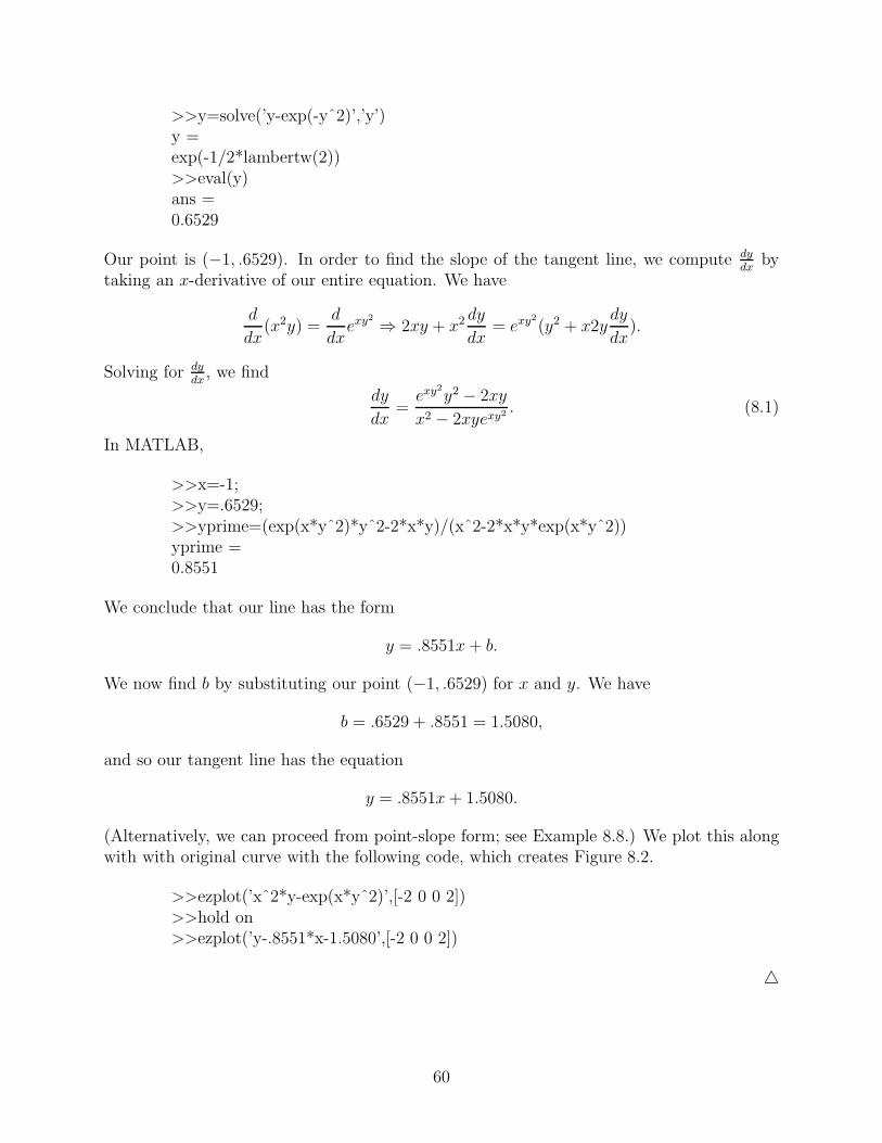
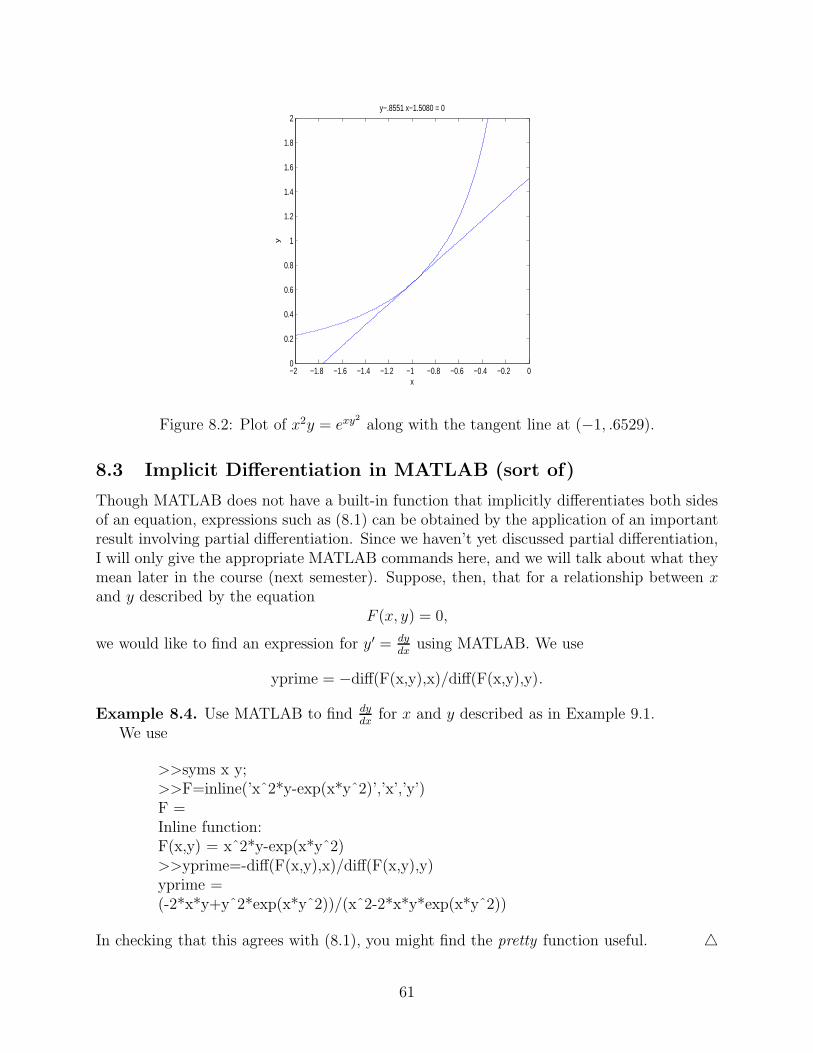
(Alternatively, we can proceed from point-slope form; see Example 8.8.) We plot this alongwith with original curve with the following code, which creates Figure 8.2.

>>ezplot(’xˆ2*y-exp(x*yˆ2)’,[-2 0 0 2])>>hold on>>ezplot(’y-.8551*x-1.5080’,[-2 0 0 2])

△

60

−2 −1.8 −1.6 −1.4 −1.2 −1 −0.8 −0.6 −0.4 −0.2 00

0.2

0.4

0.6

0.8

1

1.2

1.4

1.6

1.8

2

x

y

y−.8551 x−1.5080 = 0

Figure 8.2: Plot of x2y = exy2

along with the tangent line at (−1, .6529).

8.3 Implicit Differentiation in MATLAB (sort of)

Though MATLAB does not have a built-in function that implicitly differentiates both sidesof an equation, expressions such as (8.1) can be obtained by the application of an importantresult involving partial differentiation. Since we haven’t yet discussed partial differentiation,I will only give the appropriate MATLAB commands here, and we will talk about what theymean later in the course (next semester). Suppose, then, that for a relationship between xand y described by the equation

F (x, y) = 0,

we would like to find an expression for y′ = dy

dxusing MATLAB. We use

yprime = −diff(F(x,y),x)/diff(F(x,y),y).

Example 8.4. Use MATLAB to find dy

dxfor x and y described as in Example 9.1.

We use

>>syms x y;>>F=inline(’xˆ2*y-exp(x*yˆ2)’,’x’,’y’)F =Inline function:F(x,y) = xˆ2*y-exp(x*yˆ2)>>yprime=-diff(F(x,y),x)/diff(F(x,y),y)yprime =(-2*x*y+yˆ2*exp(x*yˆ2))/(xˆ2-2*x*y*exp(x*yˆ2))

In checking that this agrees with (8.1), you might find the pretty function useful. △

61

8.4 Assignments

1. [5 pts] Plot the relation between x and y described by the equation

x4 + y4 = 1.

Use the limits x ∈ [−2, 2] and y ∈ [−2, 2]. On the same figure, add the lines that are tangent

to this curve at the points (12,

4√

152

) and (12,

4√

152

).

2. [5 pts] Plot the relation between x and y described by the equation

x3 + y3 = 6xy.

Use the limits x ∈ [−4, 4] and y ∈ [−4, 4]. On the same figure, add the line that is tangentto this curve at the point (3, 3).

62

9 Derivatives of Exponential and Inverse Functions

9.1 Approximating e from the Definition

One definition for the natural base e is the base for which the following limit holds:

limh→0

eh − 1

h= 1.

In order to approximate a value of e from this definition, we must recall what we mean bythis limit. By our formal definition of limits, for any ǫ > 0 there exists some δ > 0 so thatif |h| < δ then

|eh − 1

h− 1| < ǫ.

(Keep in mind here that we are not proving this; we are taking advantage of it.) We have,then

−ǫ <eh − 1

h− 1 < ǫ ⇒ (1 − ǫ)h + 1 < eh < (1 + ǫ)h + 1.

Taking the 1h

power of each term in the inequality, we find that e is bounded by

((1 − ǫ)h + 1)1

h < e < ((1 + ǫ)h + 1)1

h . (9.1)

Given any ǫ > 0, we can choose h sufficiently small to make these true, so we will start withǫ = .0001, and study values of these expression as h → 0. We can compute an upper boundwith the following MATLAB code, in which the function R(ǫ, h) is simply the right-handside of (9.1). We have

>>R=inline(’((1+ep)*h+1)ˆ(1/h)’,’ep’,’h’)R =Inline function:R(ep,h) = ((1+ep)*h+1)ˆ(1/h)>>R(.0001,.01)ans =2.7051>>R(.0001,.001)ans =2.7172>>R(.0001,.0001)ans =2.7184>>R(.0001,.00001)ans =2.7185

We conclude that e < 2.7185. On the other hand, we can get a lower bound with thefollowing similar code:

63

>>L=inline(’((1-ep)*h+1)ˆ(1/h)’,’ep’,’h’)L =Inline function:L(ep,h) = ((1-ep)*h+1)ˆ(1/h)>>L(.0001,.01)ans =2.7045>>L(.0001,.001)ans =2.7167>>L(.0001,.0001)ans =2.7179>>L(.0001,.00001)ans =2.7180

In this way, we conclude2.7180 < e < 2.7185.

Of course, we can make this approximation better by choosing ǫ smaller to begin with, andthen taking smaller values of h. The exact value of e to four decimal places is e = 2.7183.

9.2 The Derivative of an Inverse Function

If a function f(x) is one-to-one and differentiable on some open interval (a, b), then theinverse function f−1(x) is one-to-one and differentiable on this same interval, and for allx ∈ (a, b)

df−1

dx(x) =

1

f ′(f−1(x)). (9.2)

Example 9.1. Show that f(x) = x3 + x + 1 is invertible on (−1, 1), and compute

df−1

dx(0).

First, we can check the invertibility of this function in MATLAB by plotting it andapplying the horizontal line test. The following code created Figure 9.1, from which it isclear that no horizontal line crosses the function more than once.

>>x=linspace(-1,1,100);>>f=x.ˆ3+x+1;>>plot(x,f)

According to (9.2), we can now compute df−1

dx(0) as

df−1

dx(0) =

1

f ′(f−1(0)),

64

−1 −0.8 −0.6 −0.4 −0.2 0 0.2 0.4 0.6 0.8 1−1

−0.5

0

0.5

1

1.5

2

2.5

3

Figure 9.1: Plot of f(x) = x3 + x + 1.

wheref ′(x) = 3x2 + 1.

All that remains is to compute f−1(0), and we observe that this is the x value associatedwith y = 0, and hence it is the real value of x that satisfies the equation

0 = x3 + x + 1.

We solve this in MATLAB with the following code:

>>solve(’xˆ3+x+1’)ans =-1/6*(108+12*93ˆ(1/2))ˆ(1/3)+2/(108+12*93ˆ(1/2))ˆ(1/3)1/12*(108+12*93ˆ(1/2))ˆ(1/3)-1/(108+12*93ˆ(1/2))ˆ(1/3)+1/2*i*3ˆ(1/2)*(-1/6*(108+12*93ˆ(1/2))ˆ(1/3)-2/(108+12*93ˆ(1/2))ˆ(1/3))1/12*(108+12*93ˆ(1/2))ˆ(1/3)-1/(108+12*93ˆ(1/2))ˆ(1/3)-1/2*i*3ˆ(1/2)*(-1/6*(108+12*93ˆ(1/2))ˆ(1/3)-2/(108+12*93ˆ(1/2))ˆ(1/3))>>eval(ans)ans =-0.68230.3412 - 1.1615i0.3412 + 1.1615i

Though the cubic equation has three roots (as expected), only one is real. (If two of theroots were real, the function would not have an inverse on this interval.) We conclude that(to four decimal places of accuracy)

f(−.6823) = 0,

65

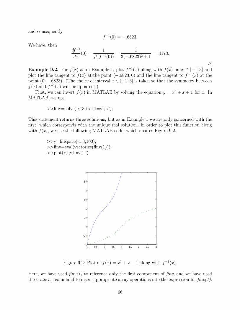
and consequentlyf−1(0) = −.6823.

We have, thendf−1

dx(0) =

1

f ′(f−1(0))=

1

3(−.6823)2 + 1= .4173.

△Example 9.2. For f(x) as in Example 1, plot f−1(x) along with f(x) on x ∈ [−1, 3] andplot the line tangent to f(x) at the point (−.6823, 0) and the line tangent to f−1(x) at thepoint (0,−.6823). (The choice of interval x ∈ [−1, 3] is taken so that the symmetry betweenf(x) and f−1(x) will be apparent.)

First, we can invert f(x) in MATLAB by solving the equation y = x3 + x + 1 for x. InMATLAB, we use.

>>finv=solve(’xˆ3+x+1=y’,’x’);

This statement returns three solutions, but as in Example 1 we are only concerned with thefirst, which corresponds with the unique real solution. In order to plot this function alongwith f(x), we use the following MATLAB code, which creates Figure 9.2.

>>y=linspace(-1,3,100);>>finv=eval(vectorize(finv(1)));>>plot(x,f,y,finv,’–’)

−1 −0.5 0 0.5 1 1.5 2 2.5 3−1

−0.5

0

0.5

1

1.5

2

2.5

3

Figure 9.2: Plot of f(x) = x3 + x + 1 along with f−1(x).

Here, we have used finv(1) to reference only the first component of finv, and we have usedthe vectorize command to insert appropriate array operations into the expression for finv(1).

66

We see from Figure 9.2 that the inverse function is simply a mirror image of the originalfunction about the line y = x. In order to plot the tangent line to f(x), we observe from ourcalculations above that the slope of this line is

m1 = f ′(−.6823) = 3(−.6823)2 + 1 = 2.3966.

The y-intercept can be found from the point (−.6823, 0),

0 = 2.3966(−.6823) + b1 ⇒ b1 = 1.6352

That is, the equation for the line tangent to f(x) at (−.6823, 0) is

y = 2.3966x + 1.6352.

On the other hand, the slope of the line tangent to f−1(x) at (0,−.6823) is m2 = .4173,as computed in Example 1. (This is also simply 1/2.3966; that is, these equations havereciprocal slopes.) In this case, we find the y-intercept b2 from

−.6823 = .4173(0) + b2 ⇒ b2 = −.6823.

That is, the equation for the line tangent to f−1(x) at the point (0,−.6823) is

y = .4173x − .6823.

Finally, we add these lines to our figure with the following MATLAB code.

>>tangent1=2.3866*x+1.6352;>>tangent2=.4173*y-.6823;>>plot(x,f,x,tangent1,’b’,y,finv,’–’,y,tangent2,’g’)>>axis([-1 3 -1 3])

The axis command has been added at the end so that the figure will have the same scaling asFigure 9.2. In order to add this command, the figure created with plot should be minimized,and then the command typed into the command window. The new figure is given as Figure9.3. △

9.3 Assignments

1. [3 pts] Proceed as in Section 9.1 and find the value of a so that

limh→0

ah − 1

h= 1.1447.

2. [2 pts] Use the derivative formula

d

dxax = ax ln a,

67

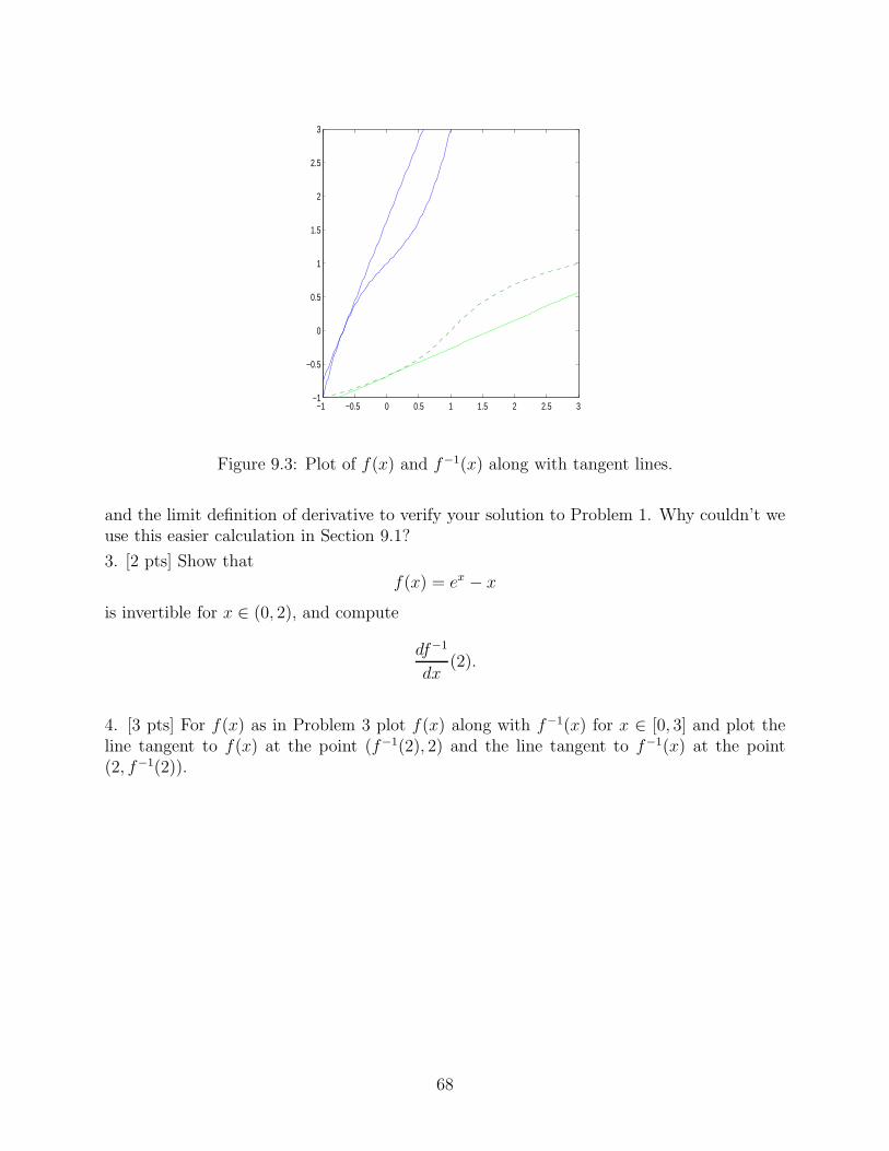
−1 −0.5 0 0.5 1 1.5 2 2.5 3−1

−0.5

0

0.5

1

1.5

2

2.5

3

Figure 9.3: Plot of f(x) and f−1(x) along with tangent lines.

and the limit definition of derivative to verify your solution to Problem 1. Why couldn’t weuse this easier calculation in Section 9.1?

3. [2 pts] Show thatf(x) = ex − x

is invertible for x ∈ (0, 2), and compute

df−1

dx(2).

4. [3 pts] For f(x) as in Problem 3 plot f(x) along with f−1(x) for x ∈ [0, 3] and plot theline tangent to f(x) at the point (f−1(2), 2) and the line tangent to f−1(x) at the point(2, f−1(2)).

68

10 Extrema and the Mean Value Theorem

10.1 The Mean Value Theorem

One of the most useful theorems in calculus is the Mean Value Theorem.

Theorem (Mean Value Theorem). Suppose f(x) is continuous on the closed interval[a, b] and differentiable on the open interval (a, b). Then there exists at least one numberc ∈ (a, b) so that

f ′(c) =f(b) − f(a)

b − a.

Example 10.1. For f(x) = x + e3x on [0, 1], find c so that

f ′(c) =f(1) − f(0)

1 − 0. (10.1)

In this case, f ′(x) = 1 + 3e3x, and so we must find c so that

1 + 3e3c =1 + e3 − 1

1= e3.

If we subtract 1 from both sides, divide by 3, and take a natural logarithm, we find

c =1

3ln(

e3 − 1

3) = .6168,

which is indeed on the open interval (0, 1).In order to understand this example graphically, we observe that (10.1) relates the slope

of the tangent line at x = c with the slope of the secant line connecting the points (0, f(0))and (1, f(1)). In the following MATLAB code, we plot three things: (1) the function f(x)on (0, 1), (2) the line tangent to f(x) at x = .6168, and (3) the secant line connecting thepoints (0, 1) and (1, 1+ e3). In order to plot the tangent line, we will require the y-intercept,which (observing from above that f ′(.6168) = e3) can be computed from

y = e3x + b,

and the observation that f(.6168) = 6.9786 so that (.6168, 6.9786) is a point on the line.That is,

6.9786 = .6168e3 + b ⇒ b = −5.4101.

Figure 10.1 is now created with the following MATLAB code.

>>x=linspace(0,1,100);>>f=x+exp(3*x);>>tangent=exp(3)*x-5.4101;>>plot(x,f,x,tangent,[0 1],[1 1+exp(3)])

We observe that the Mean Value Theorem simply asserts that there must be some pointbetween 0 and 1 so that the slope of the tangent line at that point is the same as the slopeof the secant line between the endpoints of the function. △

69

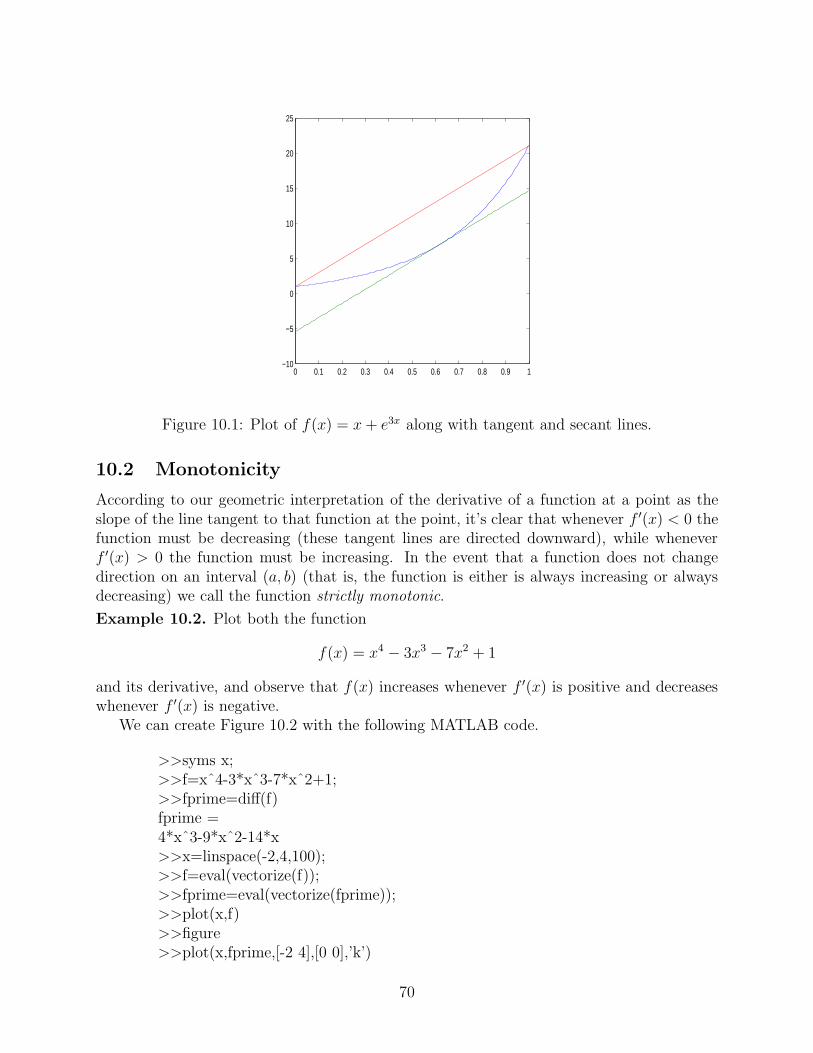
0 0.1 0.2 0.3 0.4 0.5 0.6 0.7 0.8 0.9 1−10

−5

0

5

10

15

20

25

Figure 10.1: Plot of f(x) = x + e3x along with tangent and secant lines.

10.2 Monotonicity

According to our geometric interpretation of the derivative of a function at a point as theslope of the line tangent to that function at the point, it’s clear that whenever f ′(x) < 0 thefunction must be decreasing (these tangent lines are directed downward), while wheneverf ′(x) > 0 the function must be increasing. In the event that a function does not changedirection on an interval (a, b) (that is, the function is either is always increasing or alwaysdecreasing) we call the function strictly monotonic.

Example 10.2. Plot both the function

f(x) = x4 − 3x3 − 7x2 + 1

and its derivative, and observe that f(x) increases whenever f ′(x) is positive and decreaseswhenever f ′(x) is negative.

We can create Figure 10.2 with the following MATLAB code.

>>syms x;>>f=xˆ4-3*xˆ3-7*xˆ2+1;>>fprime=diff(f)fprime =4*xˆ3-9*xˆ2-14*x>>x=linspace(-2,4,100);>>f=eval(vectorize(f));>>fprime=eval(vectorize(fprime));>>plot(x,f)>>figure>>plot(x,fprime,[-2 4],[0 0],’k’)

70

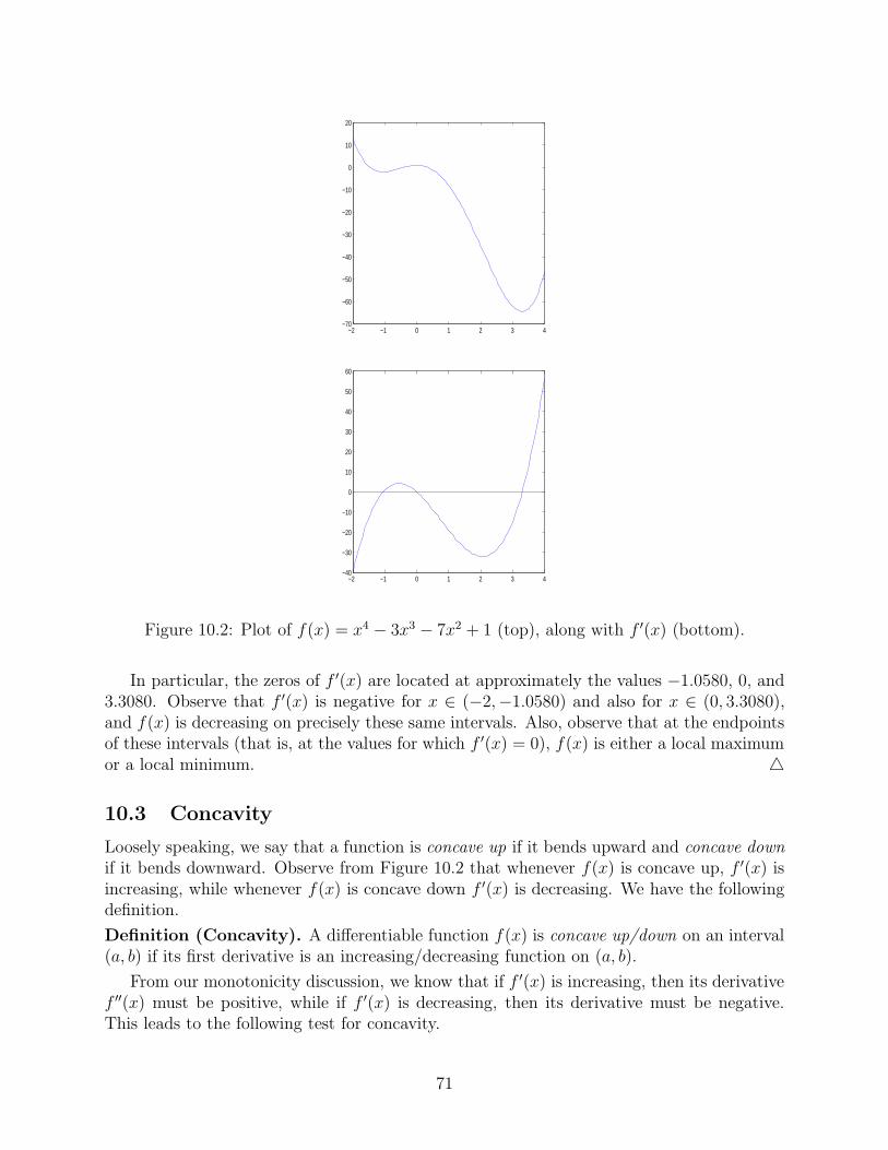
−2 −1 0 1 2 3 4−70

−60

−50

−40

−30

−20

−10

0

10

20

−2 −1 0 1 2 3 4−40

−30

−20

−10

0

10

20

30

40

50

60

Figure 10.2: Plot of f(x) = x4 − 3x3 − 7x2 + 1 (top), along with f ′(x) (bottom).

In particular, the zeros of f ′(x) are located at approximately the values −1.0580, 0, and3.3080. Observe that f ′(x) is negative for x ∈ (−2,−1.0580) and also for x ∈ (0, 3.3080),and f(x) is decreasing on precisely these same intervals. Also, observe that at the endpointsof these intervals (that is, at the values for which f ′(x) = 0), f(x) is either a local maximumor a local minimum. △

10.3 Concavity

Loosely speaking, we say that a function is concave up if it bends upward and concave downif it bends downward. Observe from Figure 10.2 that whenever f(x) is concave up, f ′(x) isincreasing, while whenever f(x) is concave down f ′(x) is decreasing. We have the followingdefinition.

Definition (Concavity). A differentiable function f(x) is concave up/down on an interval(a, b) if its first derivative is an increasing/decreasing function on (a, b).

From our monotonicity discussion, we know that if f ′(x) is increasing, then its derivativef ′′(x) must be positive, while if f ′(x) is decreasing, then its derivative must be negative.This leads to the following test for concavity.

71

Concavity Test. Suppose f(x) is twice differentiable on some interval (a, b). If f ′′(x) > 0on (a, b), then f is concave up on (a, b), while if f ′′(x) < 0 on (a, b), then f is concave downon (a, b).

Example 10.3. For f(x) as in Example 11.2, plot f(x) and f ′′(x), and observe that f(x)is concave up whenever f ′′(x) > 0 and that f(x) is concave down whenever f ′′(x) < 0. Wecan create Figure 10.3 with the following MATLAB code.

>>syms x;>>f=xˆ4-3*xˆ3-7*xˆ2+1;>>fprime2=diff(f,2)fprime2 =12*xˆ2-18*x-14>>x=linspace(-2,4,100);>>f=eval(vectorize(f));>>fprime2=eval(vectorize(fprime2));>>plot(x,f)>>figure>>plot(x,fprime2,[-2 4],[0 0],’k’)

△

10.4 Maximization and Minimization

In many applications, we are interested in finding the maximum or the minimum value of afunction over some specified interval. For example, x might denote the number of widgetsmade in some industrial process and f(x) might denote the profit drawn from the sale ofthese widgets. Since money cannot be made without the production of some widgets, weknow that f(0) = 0, while if we create too many widgets we won’t be able to sell themall, and we will lose our production costs. The goal is to find precisely the right numberof widgets to maximize our profit. The derivative is an extremely useful tool for solvingproblems of this type. Along these lines, we have the following theorem.

Fermat’s Theorem. Suppose f ′(x) is defined on some interval (a, b) and f has a localminimum or a local maximum at c ∈ (a, b). Then f ′(c) = 0.

If we combine Fermat’s Theorem with the Extreme Value Theorem, we can conclude thefollowing about the location of the global maximum and the global minimum for a functionf(x) that is continuous on a closed interval [a, b].

Categorization of Extrema. For a continuous function f on a bounded interval [a, b],suppose c is a global extremum (a global minimum or a global maximum). Then c mustsatisfy one of the following:

1. f ′(c) = 0.

2. f ′(c) does not exist.

3. c is an endpoint.

72

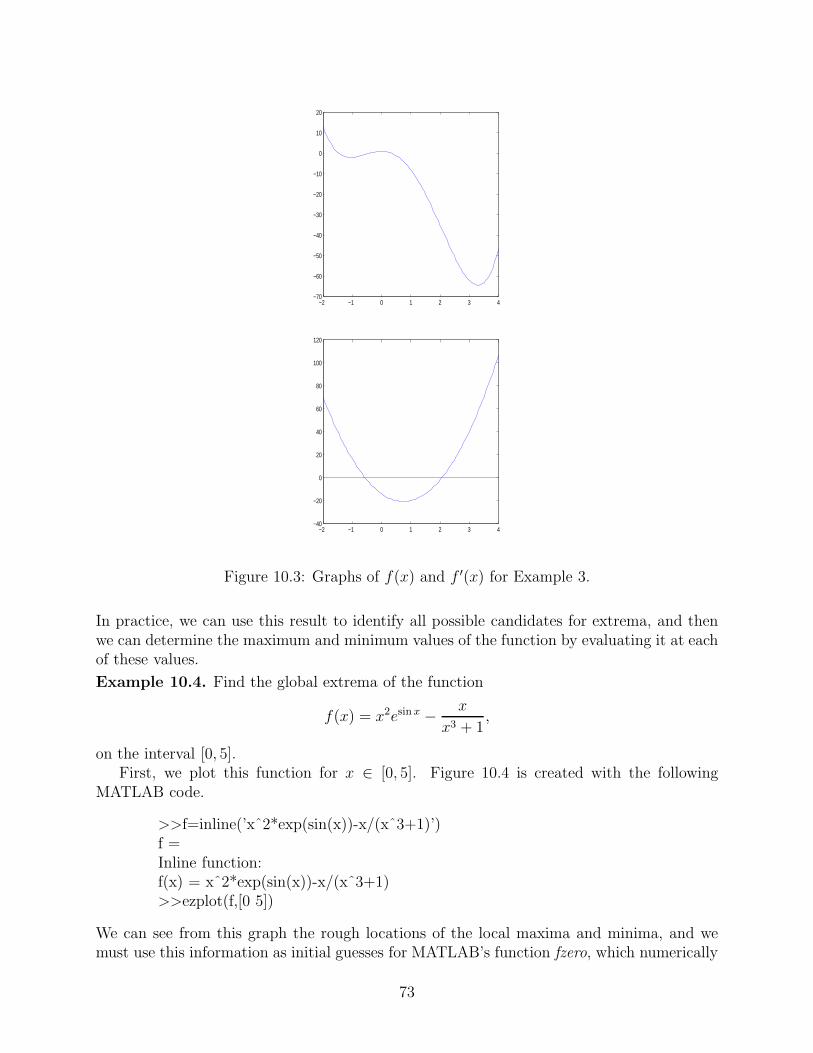
−2 −1 0 1 2 3 4−70

−60

−50

−40

−30

−20

−10

0

10

20

−2 −1 0 1 2 3 4−40

−20

0

20

40

60

80

100

120

Figure 10.3: Graphs of f(x) and f ′(x) for Example 3.

In practice, we can use this result to identify all possible candidates for extrema, and thenwe can determine the maximum and minimum values of the function by evaluating it at eachof these values.

Example 10.4. Find the global extrema of the function

f(x) = x2esin x − x

x3 + 1,

on the interval [0, 5].First, we plot this function for x ∈ [0, 5]. Figure 10.4 is created with the following

MATLAB code.

>>f=inline(’xˆ2*exp(sin(x))-x/(xˆ3+1)’)f =Inline function:f(x) = xˆ2*exp(sin(x))-x/(xˆ3+1)>>ezplot(f,[0 5])

We can see from this graph the rough locations of the local maxima and minima, and wemust use this information as initial guesses for MATLAB’s function fzero, which numerically

73

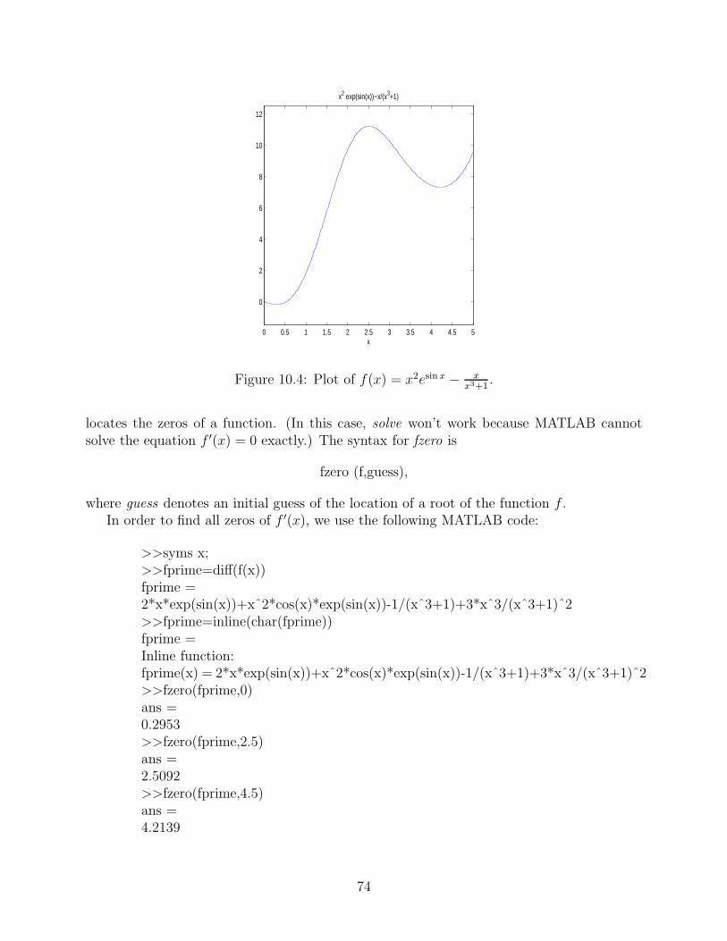
0 0.5 1 1.5 2 2.5 3 3.5 4 4.5 5

0

2

4

6

8

10

12

x

x2 exp(sin(x))−x/(x3+1)

Figure 10.4: Plot of f(x) = x2esin x − xx3+1

.

locates the zeros of a function. (In this case, solve won’t work because MATLAB cannotsolve the equation f ′(x) = 0 exactly.) The syntax for fzero is

fzero (f,guess),

where guess denotes an initial guess of the location of a root of the function f .In order to find all zeros of f ′(x), we use the following MATLAB code:

>>syms x;>>fprime=diff(f(x))fprime =2*x*exp(sin(x))+xˆ2*cos(x)*exp(sin(x))-1/(xˆ3+1)+3*xˆ3/(xˆ3+1)ˆ2>>fprime=inline(char(fprime))fprime =Inline function:fprime(x) = 2*x*exp(sin(x))+xˆ2*cos(x)*exp(sin(x))-1/(xˆ3+1)+3*xˆ3/(xˆ3+1)ˆ2>>fzero(fprime,0)ans =0.2953>>fzero(fprime,2.5)ans =2.5092>>fzero(fprime,4.5)ans =4.2139

74

Here, the command fprime=inline(char(fprime)) converts fprime into an inline function sothat it can be analyzed with the fzero command. The char command is required to convertfprime from a symbolic object into a string, which is the required input for inline. We mustnow evaluate f(x) at the five possible extrema, 0, .2953, 2.5092, 4.2139, and 5, where ofcourse the middle values are all approximate. Assuming the previous code for this examplehas already been typed in, we can evaluate f(x) at these values as follows:

>>f(0)ans =0>>f(.2953)ans =-0.1712>>f(2.5092)ans =11.2209>>f(4.2139)ans =7.3222>>f(5)ans =9.5429

We conclude that the global minimum occurs at (approximately) x = .2953, with f(.2963) =−.1712 (again approximate), and that the global maximum occurs at x = 2.5092, withf(2.5092) = 11.2209, both approximate. Of course, given our figure, we could reasonablyevaluate f only at .2953 and 2.5092, but I wanted to proceed here with a general algorithm,which consists of checking every candidate. △

10.5 Assignments

1. [3 pts] For the function f(x) = x + sin x, find the value c ∈ (0, π) so that

f ′(c) =f(π) − f(0)

π.

Plot f(x) along with the line tangent to f at the point (c, f(c)) and the secant line between(0, 0) and (π, π).

2. [2 pts] Plot f(x) = sin(2x2 − 1) along with its first derivative (as in Example 10.2) forx ∈ [0, 2π]. Specify the intervals on which f is increasing and the intervals on which f isdecreasing.

3. [2 pts] For the function from Problem 2 plot f(x) along with f ′′(x) (as in Example 10.3)for x ∈ [0, 2π]. Specify the intervals on which f is concave up and the intervals on which fis concave down.

75

4. [3 pts] Determine the absolute maximum and absolute minimum values of the function

f(x) = x5e−x2 − sin x

x2 + 1,

for x ∈ [0, 5].

76

11 Limits of Sequences

MATLAB’s symbolic toolbox has a function limit that can symbolically compute limits.

Example 11.1. Consider the exponential sequence

an = 3 · 2n, n = 0, 1, 2, 3, ....

We can computelim

n→∞an = ∞

with the following MATLAB code:

>>syms n>>limit(3*2ˆn,n,Inf)ans =Inf

△

Example 11.2. We can compute the limit

limn→∞

1

n + 1= 0


>>limit(1/(n+1),n,Inf)ans =0

△

Example 11.3. We can compute the Zeno limit

limn→∞

2n − 1

2n= 1


>>limit((2ˆn-1)/2ˆn,n,Inf)ans =1

△

77

11.1 Experimenting with the Limit Definition

In class, we made the following precise definition of a limit:

Definition. The sequence {an}∞n=1 converges to a limit a, written

limn→∞

an = a,

if for any ǫ > 0, there exists an integer N so that if n > N then |an − a| < ǫ.

Example 11.4. Consider the Zeno limit

limn→∞

2n − 1

2n= 1.

In proving that this sequence converges to 1, we must show that for any ǫ > 0 there existsan integer N so that if n > M then

|2n − 1

2n− 1| < ǫ.

We can view this graphically in MATLAB by plotting the sequence an as a function of itsindex n. At the MATLAB prompt, type

>>n=1:10;>>a=(2.ˆn-1)./(2.ˆn);>>plot(n,a,’o’)

The plot this creates is given below in Figure 11.1.We can see from Figure 11.1 that if ǫ = .1, then N = 4 is clearly sufficient. Likewise, if

ǫ = .05, then N = 5 appears to be sufficient. The choice of N depends on ǫ, and the smallerwe take ǫ to be, the larger N must be. In fact, recalling from class that in the proof thatZeno’s limit converges we took N to be the first integer larger than − log2 ǫ, we can see thedependence explicitly. In particular, we plot the function

f(ǫ) = − log2 ǫ.

>>epsilon=.001:.01:.1;>>f=-log2(epsilon);>>plot(epsilon,f)

It is clear from Figure 11.2 that as ǫ gets small, this value − log2 ǫ grows.

78

1 2 3 4 5 6 7 8 9 100.4

0.5

0.6

0.7

0.8

0.9

1

Figure 11.1: Figure for Example 4.

11.2 Recursions

We have seen in class that if we are computing population values at discrete times, wetypically find recursive schemes of calculation.

Example 11.5. Consider the Beverton–Holt recruitment curve

Nt+1 =RNt

1 + R−1K

Nt

; N(0) = N0,

where we will take the growth rate R to be 2, the carrying capacity K to be 10, and theinitial population N0 to be 1. Write a MATLAB function M-file that takes an integer valueof t as input and returns the value of the population at that time.

function value = bevholt(t)R = 2; K = 10; N0 = 1;N(1) = N0;for k = 1:tN(k+1) = R*N(k)/(1 + ((R-1)/K)*N(k));endvalue = N(t+1);

Observe that since MATLAB does not allow a 0 index, we have had to associate the index1 with the time 0, the index 2 with the time 1 etc. We can now calculuate populationsaccording to this model as follows:

>>bevholt(0)

79

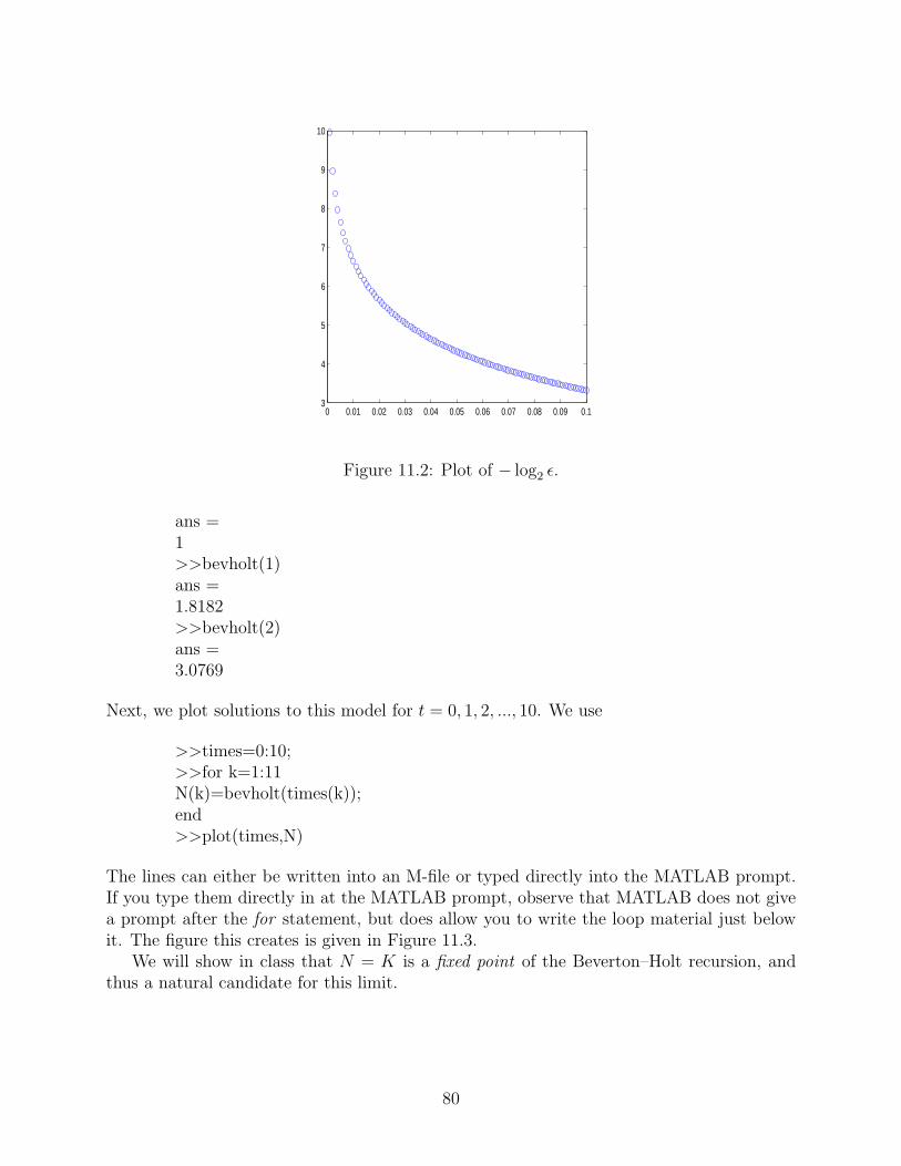
0 0.01 0.02 0.03 0.04 0.05 0.06 0.07 0.08 0.09 0.13

4

5

6

7

8

9

10

Figure 11.2: Plot of − log2 ǫ.

ans =1>>bevholt(1)ans =1.8182>>bevholt(2)ans =3.0769

Next, we plot solutions to this model for t = 0, 1, 2, ..., 10. We use

>>times=0:10;>>for k=1:11N(k)=bevholt(times(k));end>>plot(times,N)

The lines can either be written into an M-file or typed directly into the MATLAB prompt.If you type them directly in at the MATLAB prompt, observe that MATLAB does not givea prompt after the for statement, but does allow you to write the loop material just belowit. The figure this creates is given in Figure 11.3.

We will show in class that N = K is a fixed point of the Beverton–Holt recursion, andthus a natural candidate for this limit.

80

0 1 2 3 4 5 6 7 8 9 101

2

3

4

5

6

7

8

9

10

Figure 11.3: Plot of the Beverton–Holt recruitment curve.

Assignments

1. [2 pts] Compute the following limits in MATLAB:

1a.lim

N→∞(√

N −√

N − 1).

1b.

limN→∞

(1 +1

N)N .

2. [3 pts] Show that

limN→∞

N(1 − .51

N ) = ln 2

(keeping in mind that MATLAB denotes ln by log). This means that for any ǫ > 0 thereexists some integer N large enough so that

|N(1 − .51

N ) − ln 2| < ǫ.

Find such values of N for ǫ = .1 and for ǫ = .01.

3. [5 pts] Write a MATLAB function M-file that takes an integer time t as input and returnsthe population at time t according to the discrete logistic equation

Nt+1 = Nt

[

1 + R(

1 − Nt

K

)]

.

Take the growth rate R to be 2, the carrying capacity K to be 10, and the initial populationN0 to be 1. Turn in a plot depicting N(t) at the times t = 0, 1, 2, ..., 10.

81

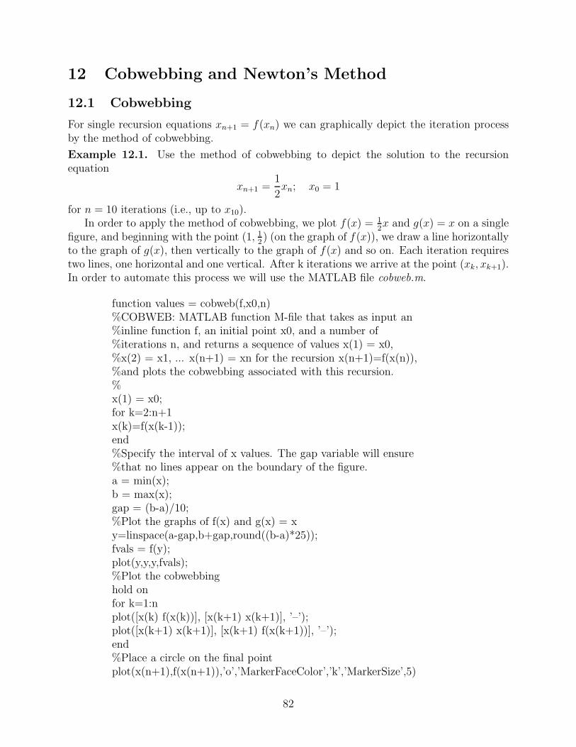
12 Cobwebbing and Newton’s Method

12.1 Cobwebbing

For single recursion equations xn+1 = f(xn) we can graphically depict the iteration processby the method of cobwebbing.

Example 12.1. Use the method of cobwebbing to depict the solution to the recursionequation

xn+1 =1

2xn; x0 = 1

for n = 10 iterations (i.e., up to x10).In order to apply the method of cobwebbing, we plot f(x) = 1

2x and g(x) = x on a single

figure, and beginning with the point (1, 12) (on the graph of f(x)), we draw a line horizontally

to the graph of g(x), then vertically to the graph of f(x) and so on. Each iteration requirestwo lines, one horizontal and one vertical. After k iterations we arrive at the point (xk, xk+1).In order to automate this process we will use the MATLAB file cobweb.m.

function values = cobweb(f,x0,n)%COBWEB: MATLAB function M-file that takes as input an%inline function f, an initial point x0, and a number of%iterations n, and returns a sequence of values x(1) = x0,%x(2) = x1, ... x(n+1) = xn for the recursion x(n+1)=f(x(n)),%and plots the cobwebbing associated with this recursion.%x(1) = x0;for k=2:n+1x(k)=f(x(k-1));end%Specify the interval of x values. The gap variable will ensure%that no lines appear on the boundary of the figure.a = min(x);b = max(x);gap = (b-a)/10;%Plot the graphs of f(x) and g(x) = xy=linspace(a-gap,b+gap,round((b-a)*25));fvals = f(y);plot(y,y,y,fvals);%Plot the cobwebbinghold onfor k=1:nplot([x(k) f(x(k))], [x(k+1) x(k+1)], ’–’);plot([x(k+1) x(k+1)], [x(k+1) f(x(k+1))], ’–’);end%Place a circle on the final pointplot(x(n+1),f(x(n+1)),’o’,’MarkerFaceColor’,’k’,’MarkerSize’,5)

82

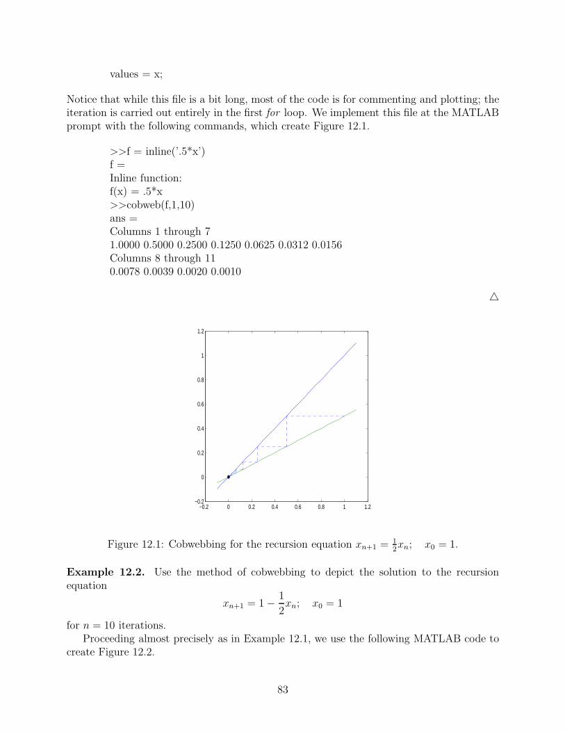
values = x;

Notice that while this file is a bit long, most of the code is for commenting and plotting; theiteration is carried out entirely in the first for loop. We implement this file at the MATLABprompt with the following commands, which create Figure 12.1.

>>f = inline(’.5*x’)f =Inline function:f(x) = .5*x>>cobweb(f,1,10)ans =Columns 1 through 71.0000 0.5000 0.2500 0.1250 0.0625 0.0312 0.0156Columns 8 through 110.0078 0.0039 0.0020 0.0010

△

−0.2 0 0.2 0.4 0.6 0.8 1 1.2−0.2

0

0.2

0.4

0.6

0.8

1

1.2

Figure 12.1: Cobwebbing for the recursion equation xn+1 = 12xn; x0 = 1.


xn+1 = 1 − 1

2xn; x0 = 1

for n = 10 iterations.Proceeding almost precisely as in Example 12.1, we use the following MATLAB code to

create Figure 12.2.

83

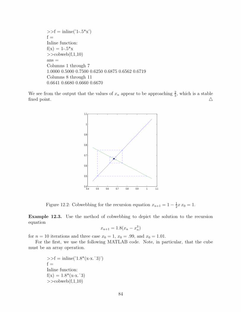
>>f = inline(’1-.5*x’)f =Inline function:f(x) = 1-.5*x>>cobweb(f,1,10)ans =Columns 1 through 71.0000 0.5000 0.7500 0.6250 0.6875 0.6562 0.6719Columns 8 through 110.6641 0.6680 0.6660 0.6670

We see from the output that the values of xn appear to be approaching 23, which is a stable

fixed point. △

0.4 0.5 0.6 0.7 0.8 0.9 1 1.10.4

0.5

0.6

0.7

0.8

0.9

1

1.1

Figure 12.2: Cobwebbing for the recursion equation xn+1 = 1 − 12xx0 = 1.


xn+1 = 1.8(xn − x3n)

for n = 10 iterations and three case x0 = 1, x0 = .99, and x0 = 1.01.For the first, we use the following MATLAB code. Note, in particular, that the cube

must be an array operation.

>>f = inline(’1.8*(x-x.ˆ3)’)f =Inline function:f(x) = 1.8*(x-x.ˆ3)>>cobweb(f,1,10)

84

ans =1 0 0 0 0 0 0 0 0 0 0

In this case x1 = 0, and 0 is recovered at every subsequent step.

−0.2 0 0.2 0.4 0.6 0.8 1 1.2−0.6

−0.4

−0.2

0

0.2

0.4

0.6

0.8

1

1.2

Figure 12.3: Cobwebbing for the recursion equation xn+1 = 1.8(xn − x3n), x0 = 1.

Next, we use the command cobweb(f,.99,10), which creates Figure 12.4. In this case,we find that a small change in the initial value x0 leads to a relatively large change in thebehavior of the system. This is a hallmark of the type of behavior defined as chaos.6 Thesystem is approaching the fixed point 2

3.

Finally, we use the command cobweb(f,1.01,10) to create Figure 12.5. We see that againthe behavior is entirely different, and in this case the system approaches the fixed point −2

3.

12.2 Newton’s Method

In Section 6 we used the bisection method to find the roots of an algebraic equation. Assecond, typically much faster method, is known as Newton’s method. Suppose we would liketo find a particular root for the equation

f(x) = 0.

We begin with an initial guess x0, and consider the line tangent to y = f(x) at x0, given inpoint-slope form by

y − f(x0) = f ′(x0)(x − x0).

6Technically, a recursion equation must have three properties to be classified as chaotic and this is onlyone of them. We haven’t developed enough theory to discuss the other two.

85

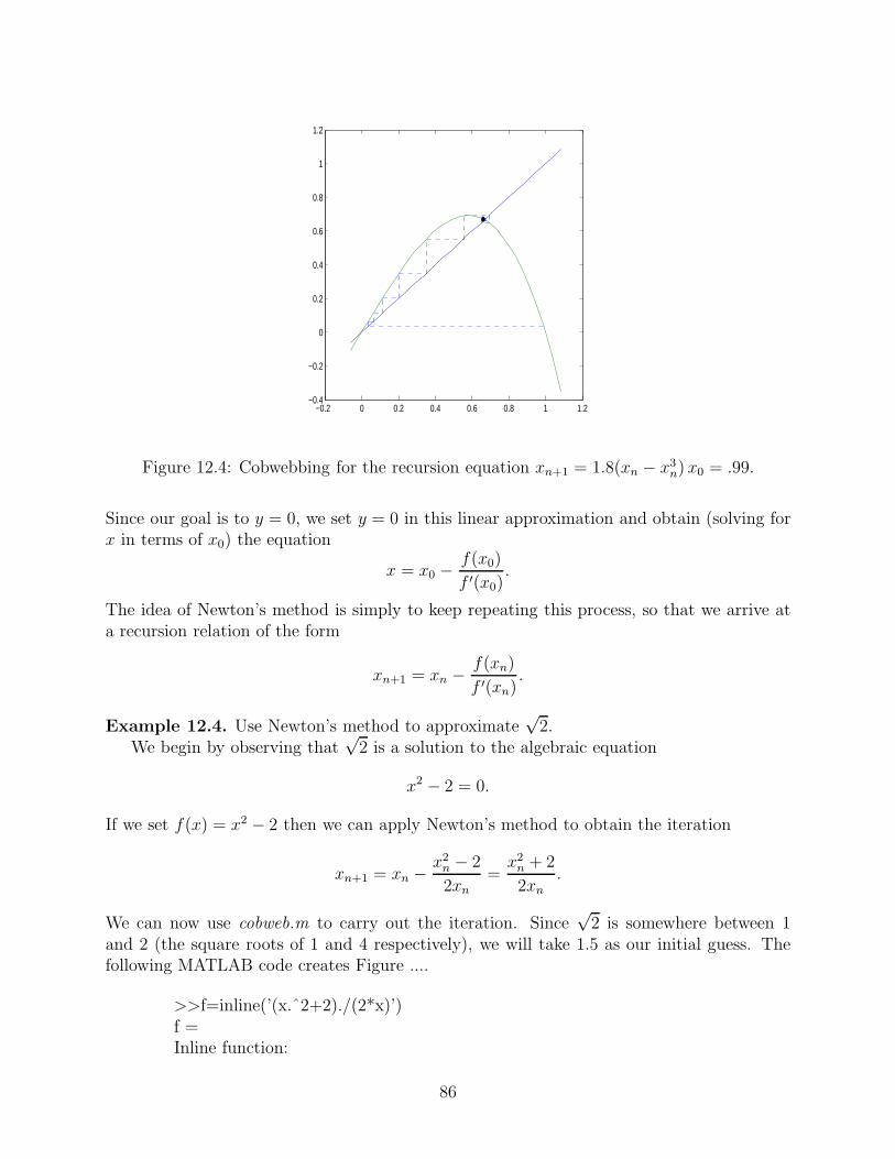
−0.2 0 0.2 0.4 0.6 0.8 1 1.2−0.4

−0.2

0

0.2

0.4

0.6

0.8

1

1.2

Figure 12.4: Cobwebbing for the recursion equation xn+1 = 1.8(xn − x3n) x0 = .99.

Since our goal is to y = 0, we set y = 0 in this linear approximation and obtain (solving forx in terms of x0) the equation

x = x0 −f(x0)

f ′(x0).

The idea of Newton’s method is simply to keep repeating this process, so that we arrive ata recursion relation of the form

xn+1 = xn − f(xn)

f ′(xn).

Example 12.4. Use Newton’s method to approximate√

2.We begin by observing that

√2 is a solution to the algebraic equation

x2 − 2 = 0.

If we set f(x) = x2 − 2 then we can apply Newton’s method to obtain the iteration

xn+1 = xn − x2n − 2

2xn

=x2

n + 2

2xn

.

We can now use cobweb.m to carry out the iteration. Since√

2 is somewhere between 1and 2 (the square roots of 1 and 4 respectively), we will take 1.5 as our initial guess. Thefollowing MATLAB code creates Figure ....

>>f=inline(’(x.ˆ2+2)./(2*x)’)f =Inline function:

86

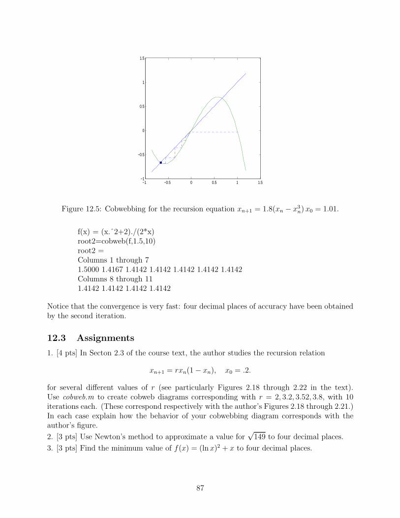
−1 −0.5 0 0.5 1 1.5−1

−0.5

0

0.5

1

1.5

Figure 12.5: Cobwebbing for the recursion equation xn+1 = 1.8(xn − x3n) x0 = 1.01.

f(x) = (x.ˆ2+2)./(2*x)root2=cobweb(f,1.5,10)root2 =Columns 1 through 71.5000 1.4167 1.4142 1.4142 1.4142 1.4142 1.4142Columns 8 through 111.4142 1.4142 1.4142 1.4142

Notice that the convergence is very fast: four decimal places of accuracy have been obtainedby the second iteration.

12.3 Assignments

1. [4 pts] In Secton 2.3 of the course text, the author studies the recursion relation

xn+1 = rxn(1 − xn), x0 = .2.

for several different values of r (see particularly Figures 2.18 through 2.22 in the text).Use cobweb.m to create cobweb diagrams corresponding with r = 2, 3.2, 3.52, 3.8, with 10iterations each. (These correspond respectively with the author’s Figures 2.18 through 2.21.)In each case explain how the behavior of your cobwebbing diagram corresponds with theauthor’s figure.

2. [3 pts] Use Newton’s method to approximate a value for√

149 to four decimal places.

3. [3 pts] Find the minimum value of f(x) = (ln x)2 + x to four decimal places.

87

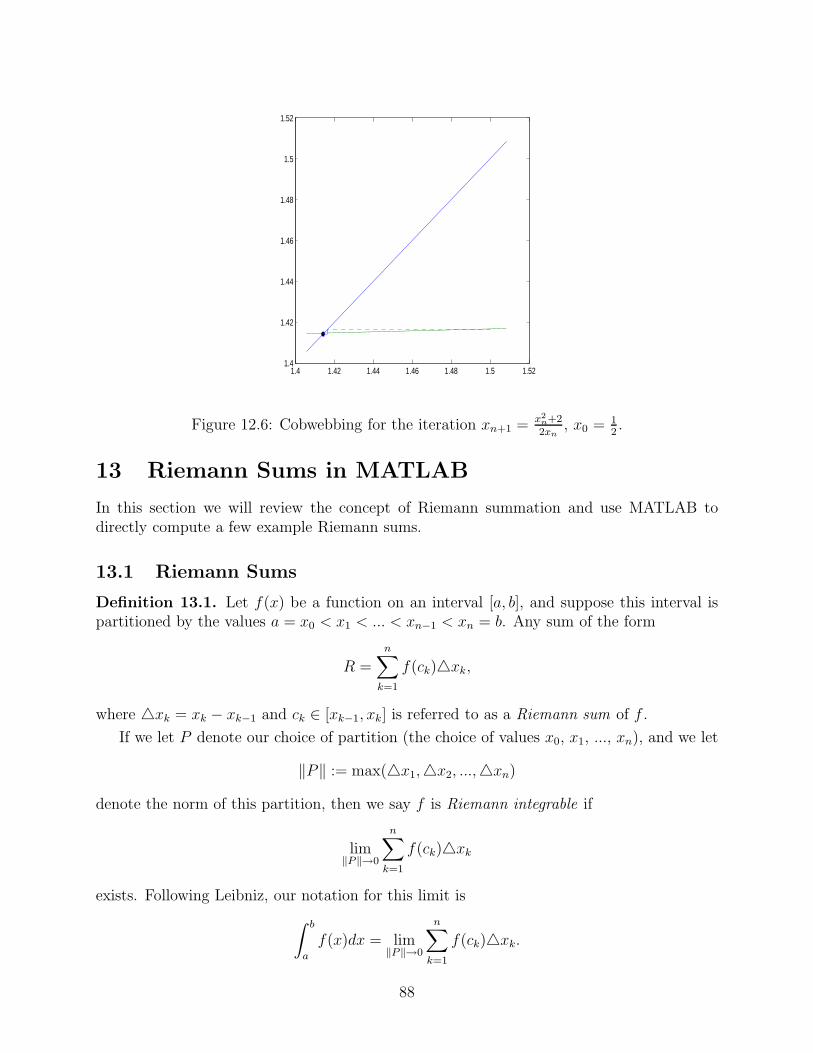
1.4 1.42 1.44 1.46 1.48 1.5 1.521.4

1.42

1.44

1.46

1.48

1.5

1.52

Figure 12.6: Cobwebbing for the iteration xn+1 = x2n+22xn

, x0 = 12.

13 Riemann Sums in MATLAB

In this section we will review the concept of Riemann summation and use MATLAB todirectly compute a few example Riemann sums.

13.1 Riemann Sums

Definition 13.1. Let f(x) be a function on an interval [a, b], and suppose this interval ispartitioned by the values a = x0 < x1 < ... < xn−1 < xn = b. Any sum of the form

R =

n∑

k=1

f(ck)△xk,

where △xk = xk − xk−1 and ck ∈ [xk−1, xk] is referred to as a Riemann sum of f .

If we let P denote our choice of partition (the choice of values x0, x1, ..., xn), and we let

‖P‖ := max(△x1,△x2, ...,△xn)

denote the norm of this partition, then we say f is Riemann integrable if

lim‖P‖→0

n∑

k=1

f(ck)△xk

exists. Following Leibniz, our notation for this limit is

∫ b

a

f(x)dx = lim‖P‖→0

n∑

k=1

f(ck)△xk.

88

Example 13.1. As our first example, we will consider the case in which ck is always chosenas the right endpoint of the interval [xk−1, xk]. If we take a regular partition with n intervals,

then each interval has length △x = b−an

, and the kth endpoint is

xk = a + k△x.

The Riemann sum becomes

R =

n∑

k=1

f(a + k△x)△x.

Suppose we would like to approximate the integral

∫ 2

0

e−x2

dx

with n = 4. We have △x = 2−04

= .5 and the values

x0 = 0

x1 = .5

x2 = 1

x3 = 1.5

x4 = 2.0.

The Riemann sum is

R =4

∑

k=1

f(0 + .5k).5 = .5(e−.52

+ e−12

+ e−1.52

+ e−22

) = .6352.

More generally, we can write a MATLAB function M-file that carries out this calculation forany function f (defined as an inline function), endpoints a and b and regular partition withn points. See rsum1.m.7

function value=rsum1(f,a,b,n)%RSUM1: Computes a Riemann Sum for the function f on%the interval [a,b] with a regular partition of n points.%The points on the intervals are chosen as the right endpoints.value = 0;dx = (b-a)/n;for k=1:nc = a+k*dx;value = value + f(c);endvalue = dx*value;

We run this in MATLAB with the following lines in the Command Window.

7The MATLAB M-files used in these notes are available from the course web site.

89

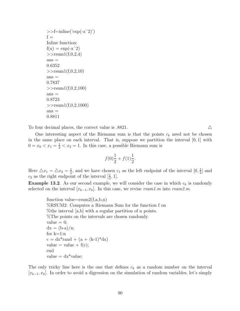
>>f=inline(’exp(-xˆ2)’)f =Inline function:f(x) = exp(-xˆ2)>>rsum1(f,0,2,4)ans =0.6352>>rsum1(f,0,2,10)ans =0.7837>>rsum1(f,0,2,100)ans =0.8723>>rsum1(f,0,2,1000)ans =0.8811

To four decimal places, the correct value is .8821. △One interesting aspect of the Riemann sum is that the points ck need not be chosen

in the same place on each interval. That is, suppose we partition the interval [0, 1] with0 = x0 < x1 = 1

2< x2 = 1. In this case, a possible Riemann sum is

f(0)1

2+ f(1)

1

2.

Here △x1 = △x2 = 12, and we have chosen c1 as the left endpoint of the interval [0, 1

2] and

c2 as the right endpoint of the interval [12, 1].

Example 13.2. As our second example, we will consider the case in which ck is randomlyselected on the interval [xk−1, xk]. In this case, we revise rsum1.m into rsum2.m.

function value=rsum2(f,a,b,n)%RSUM2: Computes a Riemann Sum for the function f on%the interval [a,b] with a regular partition of n points.%The points on the intervals are chosen randomly.value = 0;dx = (b-a)/n;for k=1:nc = dx*rand + (a + (k-1)*dx)value = value + f(c);endvalue = dx*value;

The only tricky line here is the one that defines ck as a random number on the interval[xk−1, xk]. In order to avoid a digression on the simulation of random variables, let’s simply

90

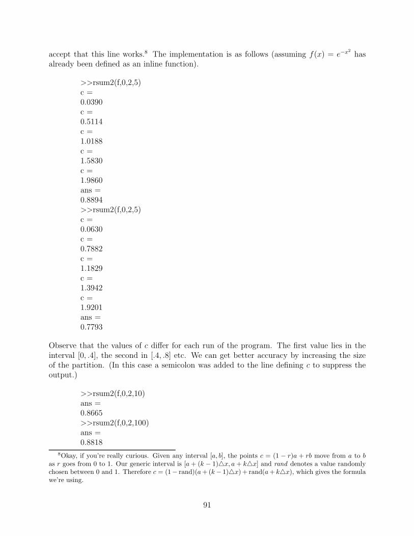
accept that this line works.8 The implementation is as follows (assuming f(x) = e−x2

hasalready been defined as an inline function).

>>rsum2(f,0,2,5)c =0.0390c =0.5114c =1.0188c =1.5830c =1.9860ans =0.8894>>rsum2(f,0,2,5)c =0.0630c =0.7882c =1.1829c =1.3942c =1.9201ans =0.7793

Observe that the values of c differ for each run of the program. The first value lies in theinterval [0, .4], the second in [.4, .8] etc. We can get better accuracy by increasing the sizeof the partition. (In this case a semicolon was added to the line defining c to suppress theoutput.)

>>rsum2(f,0,2,10)ans =0.8665>>rsum2(f,0,2,100)ans =0.8818

8Okay, if you’re really curious. Given any interval [a, b], the points c = (1 − r)a + rb move from a to b

as r goes from 0 to 1. Our generic interval is [a + (k − 1)△x, a + k△x] and rand denotes a value randomlychosen between 0 and 1. Therefore c = (1− rand)(a + (k − 1)△x) + rand(a + k△x), which gives the formulawe’re using.

91

>>rsum2(f,0,2,1000)ans =0.8821

Notice that your values may vary slightly from these due to the random nature of the pro-gram. Nonetheless, you should find that Riemann sums based on random values are actuallyconverging more rapidly to the correct solution than did Riemann sums based on right end-points. The reason for this is that when the ck are chosen randomly the area approximationson some subintervals are too large (a positive error), while the area approximations on oth-ers are too small (a negative error). Under summation, these errors can cancel, leading to abetter approximation of the total area.

13.2 Assignments

1. [5 pts] Alter the M-file rsum1.m so that it computes Riemann sums of the given functionby taking the values ck as the left endpoints of each interval. Use your M-file to estimate

∫ 2

0

e−x2

dx

for regular partitions with n = 10, 100, 1000 and compare your result with those obtainedusing right endpoints and those obtained using randomly selected points.

2. [5 pts] Alter the M-file rsum1.m so that it computes Riemann sums of the given functionby taking the values ck as the midpoints of each interval. Use your M-file to estimate

∫ 2

0

e−x2

dx

for regular partitions with n = 10, 100, 1000 and compare your result with those obtainedusing right endpoints and those obtained using randomly selected points.

92

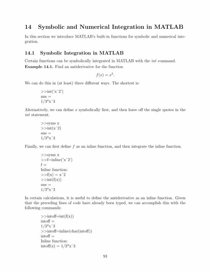
14 Symbolic and Numerical Integration in MATLAB

In this section we introduce MATLAB’s built-in functions for symbolic and numerical inte-gration.

14.1 Symbolic Integration in MATLAB

Certain functions can be symbolically integrated in MATLAB with the int command.

Example 14.1. Find an antiderivative for the function

f(x) = x2.

We can do this in (at least) three different ways. The shortest is:

>>int(’xˆ2’)ans =1/3*xˆ3

Alternatively, we can define x symbolically first, and then leave off the single quotes in theint statement.

>>syms x>>int(xˆ2)ans =1/3*xˆ3

Finally, we can first define f as an inline function, and then integrate the inline function.

>>syms x>>f=inline(’xˆ2’)f =Inline function:>>f(x) = xˆ2>>int(f(x))ans =1/3*xˆ3

In certain calculations, it is useful to define the antiderivative as an inline function. Giventhat the preceding lines of code have already been typed, we can accomplish this with thefollowing commands:

>>intoff=int(f(x))intoff =1/3*xˆ3>>intoff=inline(char(intoff))intoff =Inline function:intoff(x) = 1/3*xˆ3

93

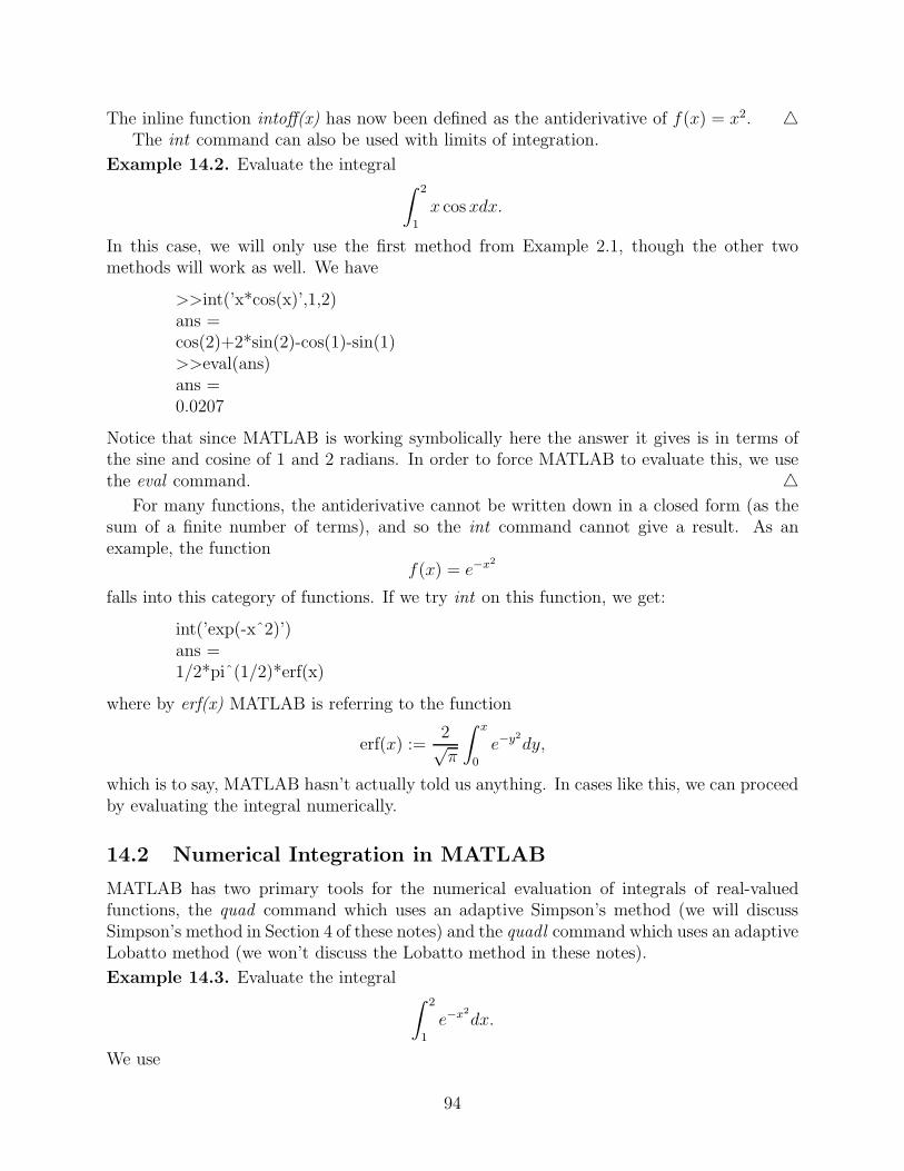
The inline function intoff(x) has now been defined as the antiderivative of f(x) = x2. △The int command can also be used with limits of integration.

Example 14.2. Evaluate the integral∫ 2

1

x cos xdx.

In this case, we will only use the first method from Example 2.1, though the other twomethods will work as well. We have

>>int(’x*cos(x)’,1,2)ans =cos(2)+2*sin(2)-cos(1)-sin(1)>>eval(ans)ans =0.0207

Notice that since MATLAB is working symbolically here the answer it gives is in terms ofthe sine and cosine of 1 and 2 radians. In order to force MATLAB to evaluate this, we usethe eval command. △

For many functions, the antiderivative cannot be written down in a closed form (as thesum of a finite number of terms), and so the int command cannot give a result. As anexample, the function

f(x) = e−x2

falls into this category of functions. If we try int on this function, we get:

int(’exp(-xˆ2)’)ans =1/2*piˆ(1/2)*erf(x)

where by erf(x) MATLAB is referring to the function

erf(x) :=2√π

∫ x

0

e−y2

dy,

which is to say, MATLAB hasn’t actually told us anything. In cases like this, we can proceedby evaluating the integral numerically.

14.2 Numerical Integration in MATLAB

MATLAB has two primary tools for the numerical evaluation of integrals of real-valuedfunctions, the quad command which uses an adaptive Simpson’s method (we will discussSimpson’s method in Section 4 of these notes) and the quadl command which uses an adaptiveLobatto method (we won’t discuss the Lobatto method in these notes).

Example 14.3. Evaluate the integral∫ 2

1

e−x2

dx.

We use

94

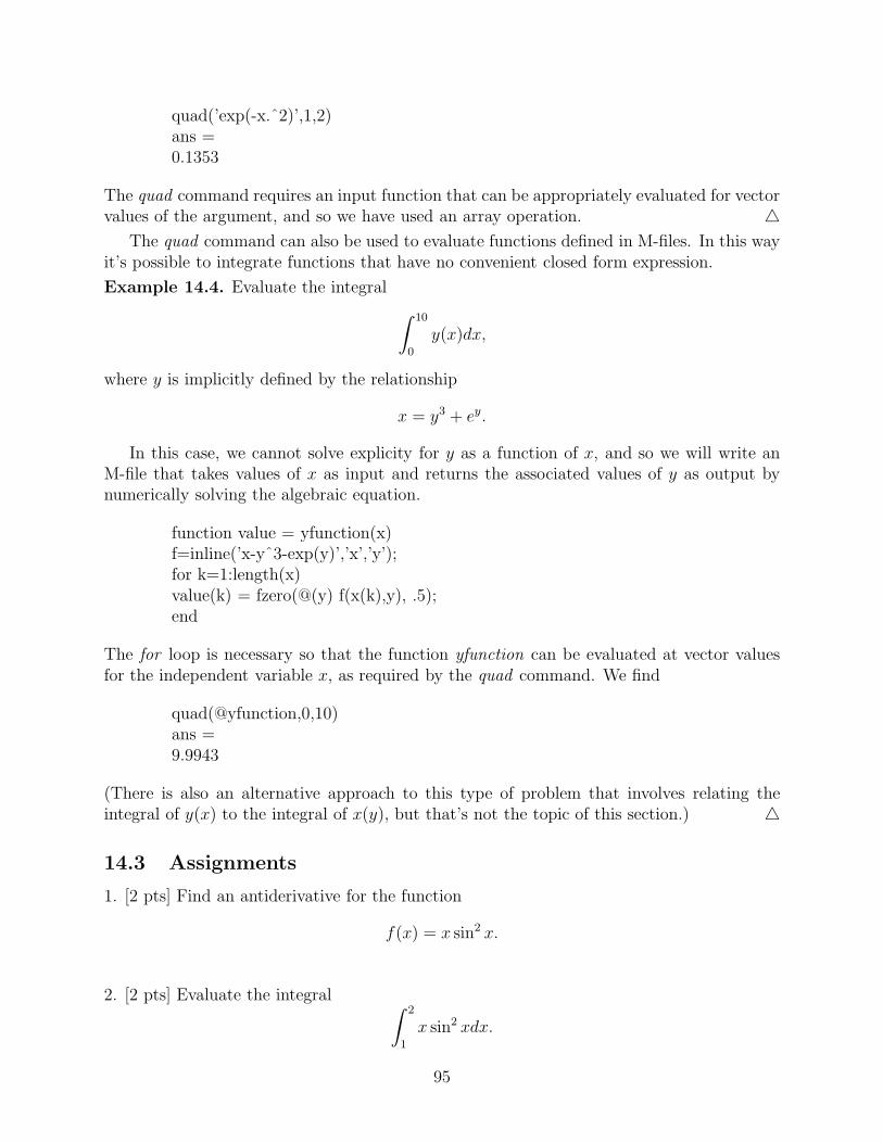
quad(’exp(-x.ˆ2)’,1,2)ans =0.1353

The quad command requires an input function that can be appropriately evaluated for vectorvalues of the argument, and so we have used an array operation. △

The quad command can also be used to evaluate functions defined in M-files. In this wayit’s possible to integrate functions that have no convenient closed form expression.

Example 14.4. Evaluate the integral

∫ 10

0

y(x)dx,

where y is implicitly defined by the relationship

x = y3 + ey.

In this case, we cannot solve explicity for y as a function of x, and so we will write anM-file that takes values of x as input and returns the associated values of y as output bynumerically solving the algebraic equation.

function value = yfunction(x)f=inline(’x-yˆ3-exp(y)’,’x’,’y’);for k=1:length(x)value(k) = fzero(@(y) f(x(k),y), .5);end

The for loop is necessary so that the function yfunction can be evaluated at vector valuesfor the independent variable x, as required by the quad command. We find

quad(@yfunction,0,10)ans =9.9943

(There is also an alternative approach to this type of problem that involves relating theintegral of y(x) to the integral of x(y), but that’s not the topic of this section.) △

14.3 Assignments

1. [2 pts] Find an antiderivative for the function

f(x) = x sin2 x.

2. [2 pts] Evaluate the integral∫ 2

1

x sin2 xdx.

95


1

sin(x2)dx.


0

y(x)dx,

where y is defined implicitly by the relation

x = y + sin y.

96

Index

axis, 18

clear, 10collect(), 11complex numbers, 10

diary, 7diff(), 50double(), 16

eval(), 16expand(), 11exporting graphs as .eps files, 25ezplot, 23

factor(), 12fplot, 34fzero(), 74

graphssaving, 25

helpdesk, 7hold on, 22horner(), 12

inline function, 33

limit(), 77linspace, 19loglog(), 30

M-Files, 33M-files

debugging, 38function, 36script, 35

multiple plots, 22

plot(), 18plots

multiple, 21pretty(), 13

real, 10

savingplots as eps, 25

semilogy(), 28simple(), 12solve(), 14structure, 15subs(), 16symbolic objects, 9

unreal, 10

vectorize(), 33

97

MATLAB for M151B - Texas A&M University

Documents

Transcript of MATLAB for M151B - Texas A&M University