1

Matlab Basics Tutorial Vectors

Functions

Plotting

Polynomials

Matrices

Printing

Using M-files in Matlab

Getting help in Matlab

Matlab Commands List

The following list of commands can be very useful for future reference. Use "help" in Matlab for more

information on how to use the commands.

In these tutorials, we use commands both from Matlab and from the Control Systems Toolbox, as well as

some commands/functions which we wrote ourselves. For those commands/functions which are not

standard in Matlab, we give links to their descriptions. For more information on writing Matlab functions,

see the function page.

Note:Matlab commands from the control system toolbox are highlighted in red.

Non-standard Matlab commands are highlighted in green.

Command Description

abs Absolute value

acker Compute the K matrix to place the poles of A-BK, see also place

axis Set the scale of the current plot, see also plot, figure

bode Draw the Bode plot, see also logspace, margin, nyquist1

c2dm Continuous system to discrete system

clf Clear figure (use clg in Matlab 3.5)

conv Convolution (useful for multiplying polynomials), see also deconv

ctrb The controllability matrix, see also obsv

deconv Deconvolution and polynomial division, see also conv

det Find the determinant of a matrix

dimpulse Impulse response of discrete-time linear systems, see also dstep

dlqr Linear-quadratic requlator design for discrete-time systems, see also lqr

dlsim Simulation of discrete-time linear systems, see also lsim

dstep Step response of discrete-time linear systems, see also stairs

eig Compute the eigenvalues of a matrix

eps Matlab's numerical tolerance

feedback Feedback connection of two systems.

figure Create a new figure or redefine the current figure, see also subplot, axis

for For, next loop

format Number format (significant digits, exponents)

function Creates function m-files

2

Command Description

grid Draw the grid lines on the current plot

gtext Add a piece of text to the current plot, see also text

help HELP!

hold Hold the current graph, see also figure

if Conditionally execute statements

imag Returns the imaginary part of a complex number, see also real

impulse Impulse response of continuous-time linear systems, see also step, lsim, dlsim

input Prompt for user input

inv Find the inverse of a matrix

jgrid Generate grid lines of constant damping ratio (zeta) and settling time (sigma), see also sgrid,

sigrid, zgrid

legend Graph legend

length Length of a vector, see also size

linspace Returns a linearly spaced vector

lnyquist1 Produce a Nyquist plot on a logarithmic scale, see also nyquist1

log natural logarithm, also log10: common logarithm

loglog Plot using log-log scale, also semilogx/semilogy

logspace Returns a logarithmically spaced vector

lqr Linear quadratic regulator design for continuous systems, see also dlqr

lsim Simulate a linear system, see also step, impulse, dlsim.

margin Returns the gain margin, phase margin, and crossover frequencies, see also bode

norm Norm of a vector

nyquist1 Draw the Nyquist plot, see also lnyquist1. Note this command was written to replace the

Matlab standard command nyquist to get more accurate Nyquist plots.

obsv The observability matrix, see also ctrb

ones Returns a vector or matrix of ones, see also zeros

place Compute the K matrix to place the poles of A-BK, see also acker

plot Draw a plot, see also figure, axis, subplot.

poly Returns the characteristic polynomial

polyadd Add two different polynomials

polyval Polynomial evaluation

print Print the current plot (to a printer or postscript file)

pzmap Pole-zero map of linear systems

rank Find the number of linearly independent rows or columns of a matrix

real Returns the real part of a complex number, see also imag

rlocfind Find the value of k and the poles at the selected point

rlocus Draw the root locus

roots Find the roots of a polynomial

rscale Find the scale factor for a full-state feedback system

set Set(gca,'Xtick',xticks,'Ytick',yticks) to control the number and spacing of tick marks on the

axes

3

Command Description

series Series interconnection of Linear time-independent systems

sgrid Generate grid lines of constant damping ratio (zeta) and natural frequency (Wn), see also

jgrid, sigrid, zgrid

sigrid Generate grid lines of constant settling time (sigma), see also jgrid, sgrid, zgrid

size Gives the dimension of a vector or matrix, see also length

sqrt Square root

ss Create state-space models or convert LTI model to state space, see also tf

ss2tf State-space to transfer function representation, see also tf2ss

ss2zp State-space to pole-zero representation, see also zp2ss

stairs Stairstep plot for discreste response, see also dstep

step Plot the step response, see also impulse, lsim, dlsim.

subplot Divide the plot window up into pieces, see also plot, figure

text Add a piece of text to the current plot, see also title, xlabel, ylabel, gtext

tf Creation of transfer functions or conversion to transfer function, see also ss

tf2ss Transfer function to state-space representation, see also ss2tf

tf2zp Transfer function to Pole-zero representation, see also zp2tf

title Add a title to the current plot

wbw Returns the bandwidth frequency given the damping ratio and the rise or settling time.

xlabel/ylabel Add a label to the horizontal/vertical axis of the current plot, see also title, text, gtext

zeros Returns a vector or matrix of zeros

zgrid Generates grid lines of constant damping ratio (zeta) and natural frequency (Wn), see also

sgrid, jgrid, sigrid

zp2ss Pole-zero to state-space representation, see also ss2zp

zp2tf Pole-zero to transfer function representation, see also tf2zp

Key Matlab Commands used in this tutorial are: plot polyval roots conv deconv polyadd inv eig poly

Note: Non-standard Matlab commands used in this tutorials are highlighted in green.

Matlab is an interactive program for numerical computation and data visualization; it is used extensively by

control engineers for analysis and design. There are many different toolboxes available which extend the

basic functions of Matlab into different application areas; in these tutorials, we will make extensive use of

the Control Systems Toolbox. Matlab is supported on Unix, Macintosh, and Windows environments; a

student version of Matlab is available for personal computers. For more information on Matlab, contact the

Mathworks.

The idea behind these tutorials is that you can view them in one window while running Matlab

in another window. You should be able to re-do all of the plots and calculations in the tutorials

by cutting and pasting text from the tutorials into Matlab or an m-file.

Vectors

Let's start off by creating something simple, like a vector. Enter each element of the vector (separated by a

space) between brackets, and set it equal to a variable. For example, to create the vector a, enter into the

Matlab command window (you can "copy" and "paste" from your browser into Matlab to make it easy):

a = [1 2 3 4 5 6 9 8 7]

4

Matlab should return:

a =

1 2 3 4 5 6 9 8 7

Let's say you want to create a vector with elements between 0 and 20 evenly spaced in increments of 2 (this

method is frequently used to create a time vector):

t = 0:2:20

t =

0 2 4 6 8 10 12 14 16 18 20

Manipulating vectors is almost as easy as creating them. First, suppose you would like to add 2 to each of

the elements in vector 'a'. The equation for that looks like:

b = a + 2

b =

3 4 5 6 7 8 11 10 9

Now suppose, you would like to add two vectors together. If the two vectors are the same length, it is easy.

Simply add the two as shown below:

c = a + b

c =

4 6 8 10 12 14 20 18 16

Subtraction of vectors of the same length works exactly the same way.

Functions

To make life easier, Matlab includes many standard functions. Each function is a block of code that

accomplishes a specific task. Matlab contains all of the standard functions such as sin, cos, log, exp, sqrt, as

well as many others. Commonly used constants such as pi, and i or j for the square root of -1, are also

incorporated into Matlab.

sin(pi/4)

ans =

0.7071

To determine the usage of any function, type help [function name] at the Matlab command window.

Matlab even allows you to write your own functions with the function command; follow the link to learn

how to write your own functions and see a listing of the functions we created for this tutorial.

Plotting

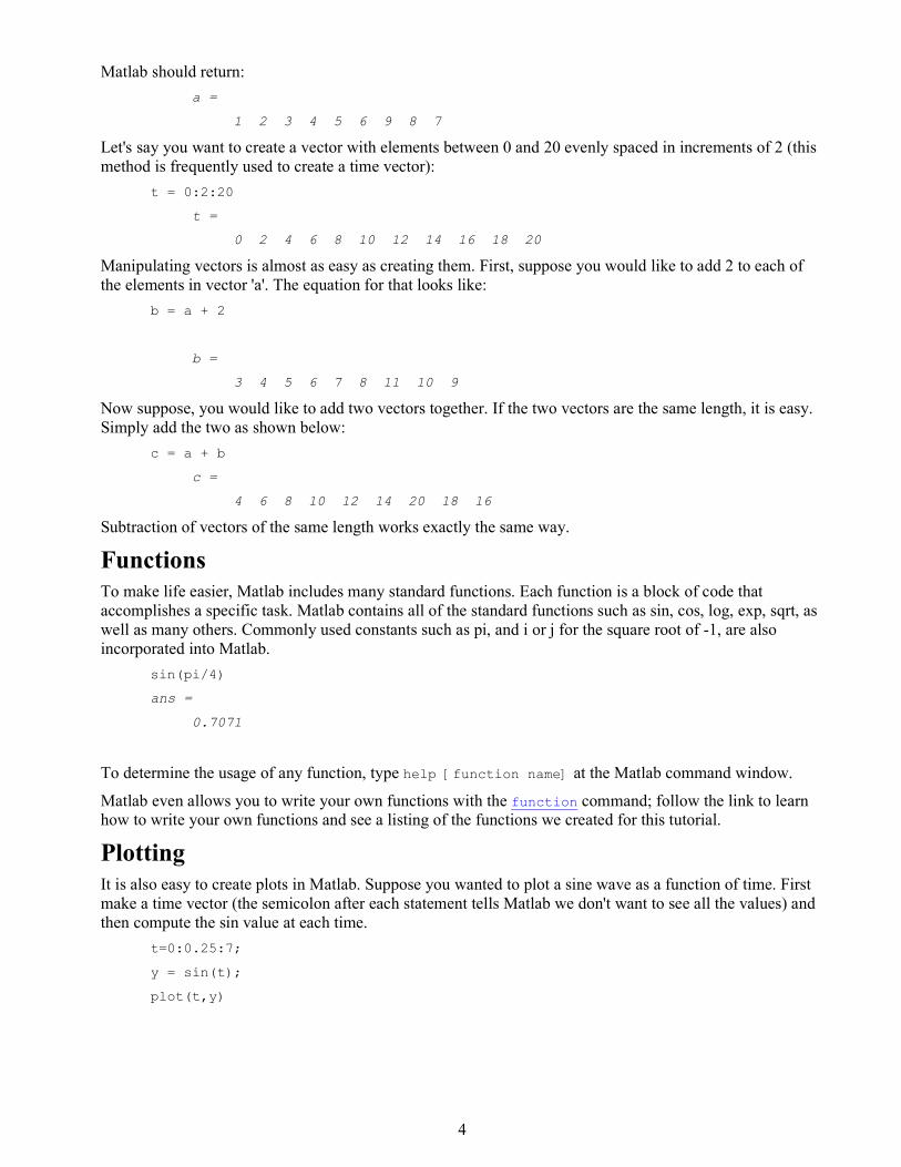
It is also easy to create plots in Matlab. Suppose you wanted to plot a sine wave as a function of time. First

make a time vector (the semicolon after each statement tells Matlab we don't want to see all the values) and

then compute the sin value at each time.

t=0:0.25:7;

y = sin(t);

plot(t,y)

5

The plot contains approximately one period of a sine wave. Basic plotting is very easy in Matlab, and the

plot command has extensive add-on capabilities. I would recommend you visit the plotting page to learn

more about it.

Polynomials

In Matlab, a polynomial is represented by a vector. To create a polynomial in Matlab, simply enter each

coefficient of the polynomial into the vector in descending order. For instance, let's say you have the

following polynomial:

To enter this into Matlab, just enter it as a vector in the following manner

x = [1 3 -15 -2 9]

x =

1 3 -15 -2 9

Matlab can interpret a vector of length n+1 as an nth order polynomial. Thus, if your polynomial is missing

any coefficients, you must enter zeros in the appropriate place in the vector. For example,

would be represented in Matlab as:

y = [1 0 0 0 1]

You can find the value of a polynomial using the polyval function. For example, to find the value of the

above polynomial at s=2,

z = polyval([1 0 0 0 1],2)

z =

17

You can also extract the roots of a polynomial. This is useful when you have a high-order polynomial such

as

Finding the roots would be as easy as entering the following command;

roots([1 3 -15 -2 9])

ans =

-5.5745

2.5836

6

-0.7951

0.7860

Let's say you want to multiply two polynomials together. The product of two polynomials is found by taking

the convolution of their coefficients. Matlab's function conv that will do this for you.

x = [1 2];

y = [1 4 8];

z = conv(x,y)

z =

1 6 16 16

Dividing two polynomials is just as easy. The deconv function will return the remainder as well as the

result. Let's divide z by y and see if we get x.

[xx, R] = deconv(z,y)

xx =

1 2

R =

0 0 0 0

As you can see, this is just the polynomial/vector x from before. If y had not gone into z evenly, the

remainder vector would have been something other than zero.

If you want to add two polynomials together which have the same order, a simple z=x+y will work (the

vectors x and y must have the same length). In the general case, the user-defined function, polyadd can be

used. To use polyadd, copy the function into an m-file, and then use it just as you would any other function

in the Matlab toolbox. Assuming you had the polyadd function stored as a m-file, and you wanted to add the

two uneven polynomials, x and y, you could accomplish this by entering the command:

z = polyadd(x,y)

x =

1 2

y =

1 4 8

z =

1 5 10

Matrices

Entering matrices into Matlab is the same as entering a vector, except each row of elements is separated by a

semicolon (;) or a return:

B = [1 2 3 4;5 6 7 8;9 10 11 12]

B =

1 2 3 4

5 6 7 8

9 10 11 12

B = [ 1 2 3 4

5 6 7 8

7

9 10 11 12]

B =

1 2 3 4

5 6 7 8

9 10 11 12

Matrices in Matlab can be manipulated in many ways. For one, you can find the transpose of a matrix using

the apostrophe key:

C = B'

C =

1 5 9

2 6 10

3 7 11

4 8 12

It should be noted that if C had been complex, the apostrophe would have actually given the complex

conjugate transpose. To get the transpose, use .' (the two commands are the same if the matix is not

complex).

Now you can multiply the two matrices B and C together. Remember that order matters when multiplying

matrices.

D = B * C

D =

30 70 110

70 174 278

110 278 446

D = C * B

D =

107 122 137 152

122 140 158 176

137 158 179 200

152 176 200 224

Another option for matrix manipulation is that you can multiply the corresponding elements of two matrices

using the .* operator (the matrices must be the same size to do this).

E = [1 2;3 4]

F = [2 3;4 5]

G = E .* F

E =

1 2

3 4

F =

2 3

4 5

G =

2 6

8

12 20

If you have a square matrix, like E, you can also multiply it by itself as many times as you like by raising it

to a given power.

E^3

ans =

37 54

81 118

If wanted to cube each element in the matrix, just use the element-by-element cubing.

E.^3

ans =

1 8

27 64

You can also find the inverse of a matrix:

X = inv(E)

X =

-2.0000 1.0000

1.5000 -0.5000

or its eigenvalues:

eig(E)

ans =

-0.3723

5.3723

There is even a function to find the coefficients of the characteristic polynomial of a matrix. The "poly"

function creates a vector that includes the coefficients of the characteristic polynomial.

p = poly(E)

p =

1.0000 -5.0000 -2.0000

Remember that the eigenvalues of a matrix are the same as the roots of its characteristic polynomial:

roots(p)

ans =

5.3723

-0.3723

Printing

Printing in Matlab is pretty easy. Just follow the steps illustrated below:

Macintosh

To print a plot or a m-file from a Macintosh, just click on the plot or m-file, select Print under the

File menu, and hit return.

Windows

9

To print a plot or a m-file from a computer running Windows, just selct Print from the File menu in

the window of the plot or m-file, and hit return.

Unix

To print a plot on a Unix workstation enter the command:

print -P<printername>

If you want to save the plot and print it later, enter the command:

print plot.ps

Sometime later, you could print the plot using the command "lpr -P plot.ps" If you are using a HP

workstation to print, you would instead use the command "lpr -d plot.ps"

To print a m-file, just print it the way you would any other file, using the command "lpr -P <name of

m-file>.m" If you are using a HP workstation to print, you would instead use the command "lpr -d

plot.ps<name of m-file>.m"

Using M-files in Matlab

There are slightly different things you need to know for each platform.

Macintosh

There is a built-in editor for m-files; choose "New M-file" from the File menu. You can also use any

other editor you like (but be sure to save the files in text format and load them when you start

Matlab).

Windows

Running Matlab from Windows is very similar to running it on a Macintosh. However, you need to

know that your m-file will be saved in the clipboard. Therefore, you must make sure that it is saved

as filename.m

Unix

You will need to run an editor separately from Matlab. The best strategy is to make a directory for

all your m-files, then cd to that directory before running both Matlab and the editor. To start Matlab

from your Xterm window, simply type: matlab.

You can either type commands directly into matlab, or put all of the commands that you will need together

in an m-file, and just run the file. If you put all of your m-files in the same directory that you run matlab

from, then matlab will always find them.

Getting help in Matlab

Matlab has a fairly good on-line help; type

help commandname

for more information on any given command. You do need to know the name of the command that you are

looking for; a list of the all the ones used in these tutorials is given in the command listing; a link to this

page can be found at the bottom of every tutorial and example page.

Here are a few notes to end this tutorial.

You can get the value of a particular variable at any time by typing its name.

B

B =

1 2 3

4 5 6

7 8 9

10

You can also have more that one statement on a single line, so long as you separate them with either a

semicolon or comma.

Also, you may have noticed that so long as you don't assign a variable a specific operation or result, Matlab

with store it in a temporary variable called "ans".

11

Modeling Tutorial Train system

Free body diagram and Newton's law

State-variable and output equations

Matlab representation

Matlab can be used to represent a physical system or a model. To begin with, let's start with a review of how

to represent a physical system as a set of differential equations.

Train system

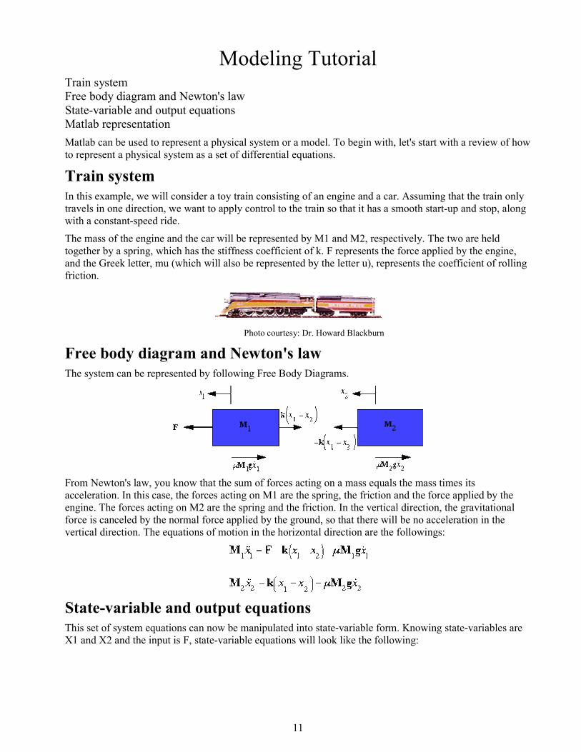
In this example, we will consider a toy train consisting of an engine and a car. Assuming that the train only

travels in one direction, we want to apply control to the train so that it has a smooth start-up and stop, along

with a constant-speed ride.

The mass of the engine and the car will be represented by M1 and M2, respectively. The two are held

together by a spring, which has the stiffness coefficient of k. F represents the force applied by the engine,

and the Greek letter, mu (which will also be represented by the letter u), represents the coefficient of rolling

friction.

Photo courtesy: Dr. Howard Blackburn

Free body diagram and Newton's law

The system can be represented by following Free Body Diagrams.

From Newton's law, you know that the sum of forces acting on a mass equals the mass times its

acceleration. In this case, the forces acting on M1 are the spring, the friction and the force applied by the

engine. The forces acting on M2 are the spring and the friction. In the vertical direction, the gravitational

force is canceled by the normal force applied by the ground, so that there will be no acceleration in the

vertical direction. The equations of motion in the horizontal direction are the followings:

State-variable and output equations

This set of system equations can now be manipulated into state-variable form. Knowing state-variables are

X1 and X2 and the input is F, state-variable equations will look like the following:

12

Let the output of the system be the velocity of the engine. Then the output equation will become:

1. Transfer function

To find the transfer funciton of the system, first, take Laplace transforms of above state-variable and output

equations.

Using these equations, derive the transfer function Y(s)/F(s) in terms of constants. When finding the

transfer function, zero initial conditions must be assumed. The transfer function should look like the one

shown below.

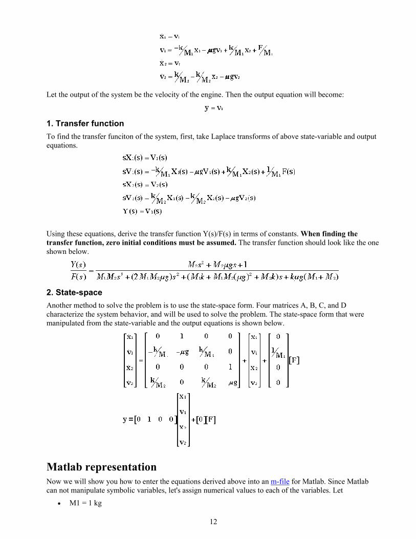
2. State-space

Another method to solve the problem is to use the state-space form. Four matrices A, B, C, and D

characterize the system behavior, and will be used to solve the problem. The state-space form that were

manipulated from the state-variable and the output equations is shown below.

Matlab representation

Now we will show you how to enter the equations derived above into an m-file for Matlab. Since Matlab

can not manipulate symbolic variables, let's assign numerical values to each of the variables. Let

• M1 = 1 kg

13

• M2 = 0.5 kg

• k = 1 N/sec

• F= 1 N

• u = 0.002 sec/m

• g = 9.8 m/s^2

Create an new m-file and enter the following commands.

M1=1;

M2=0.5;

k=1;

F=1;

u=0.002;

g=9.8;

Now you have one of two choices: 1) Use the transfer function, or 2) Use the state-space form to solve the

problem. If you choose to use the transfer function, add the following commands onto the end of the m-file

which you have just created.

num=[M2 M2*u*g 1];

den=[M1*M2 2*M1*M2*u*g M1*k+M1*M2*u*u*g*g+M2*k M1*k*u*g+M2*k*u*g];

If you choose to use the state-space form, add the following commands at the end of the m-file, instead of

num and den matrices shown above.

A=[ 0 1 0 0;

-k/M1 -u*g k/M1 0;

0 0 0 1;

k/M2 0 -k/M2 -u*g];

B=[ 0;

1/M1;

0;

0];

C=[0 1 0 0];

D=[0];

See the Matlab basics tutorial to learn more about entering matrices.

Continue solving the problem

Now, you are ready to obtain the system output (with an addition of few more commands). It should be

noted that many operations can be done using either the transfer function or the state-space model.

Furthermore, it is simple to transfer between the two if the other form of representation is required. If you

need to learn how to convert from one representation to the other, click Conversion.

This tutorial contain seven examples which allows you to learn more about modeling. You can link to them

from below.

14

PID Tutorial Introduction

The three-term controller

The characteristics of P, I, and D controllers

Example Problem

Open-loop step response

Proportional control

Proportional-Derivative control

Proportional-Integral control

Proportional-Integral-Derivative control

General tips for designing a PID controller

Key Matlab Commands used in this tutorial are: step cloop

Note: Matlab commands from the control system toolbox are highlighted in red.

Introduction

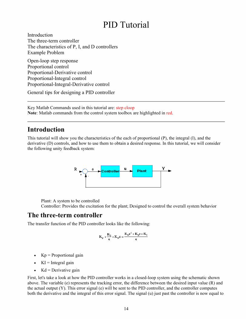
This tutorial will show you the characteristics of the each of proportional (P), the integral (I), and the

derivative (D) controls, and how to use them to obtain a desired response. In this tutorial, we will consider

the following unity feedback system:

Plant: A system to be controlled

Controller: Provides the excitation for the plant; Designed to control the overall system behavior

The three-term controller

The transfer function of the PID controller looks like the following:

• Kp = Proportional gain

• KI = Integral gain

• Kd = Derivative gain

First, let's take a look at how the PID controller works in a closed-loop system using the schematic shown

above. The variable (e) represents the tracking error, the difference between the desired input value (R) and

the actual output (Y). This error signal (e) will be sent to the PID controller, and the controller computes

both the derivative and the integral of this error signal. The signal (u) just past the controller is now equal to

15

the proportional gain (Kp) times the magnitude of the error plus the integral gain (Ki) times the integral of

the error plus the derivative gain (Kd) times the derivative of the error.

This signal (u) will be sent to the plant, and the new output (Y) will be obtained. This new output (Y) will

be sent back to the sensor again to find the new error signal (e). The controller takes this new error signal

and computes its derivative and its integral again. This process goes on and on.

The characteristics of P, I, and D controllers

A proportional controller (Kp) will have the effect of reducing the rise time and will reduce ,but never

eliminate, the steady-state error. An integral control (Ki) will have the effect of eliminating the steady-state

error, but it may make the transient response worse. A derivative control (Kd) will have the effect of

increasing the stability of the system, reducing the overshoot, and improving the transient response. Effects

of each of controllers Kp, Kd, and Ki on a closed-loop system are summarized in the table shown below.

CL RESPONSE RISE TIME OVERSHOOT SETTLING TIME S-S ERROR

Kp Decrease Increase Small Change Decrease

Ki Decrease Increase Increase Eliminate

Kd Small Change Decrease Decrease Small Change

Note that these correlations may not be exactly accurate, because Kp, Ki, and Kd are dependent of each

other. In fact, changing one of these variables can change the effect of the other two. For this reason, the

table should only be used as a reference when you are determining the values for Ki, Kp and Kd.

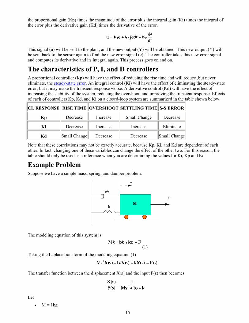
Example Problem

Suppose we have a simple mass, spring, and damper problem.

The modeling equation of this system is

(1)

Taking the Laplace transform of the modeling equation (1)

The transfer function between the displacement X(s) and the input F(s) then becomes

Let

• M = 1kg

16

• b = 10 N.s/m

• k = 20 N/m

• F(s) = 1

Plug these values into the above transfer function

The goal of this problem is to show you how each of Kp, Ki and Kd contributes to obtain

• Fast rise time

• Minimum overshoot

• No steady-state error

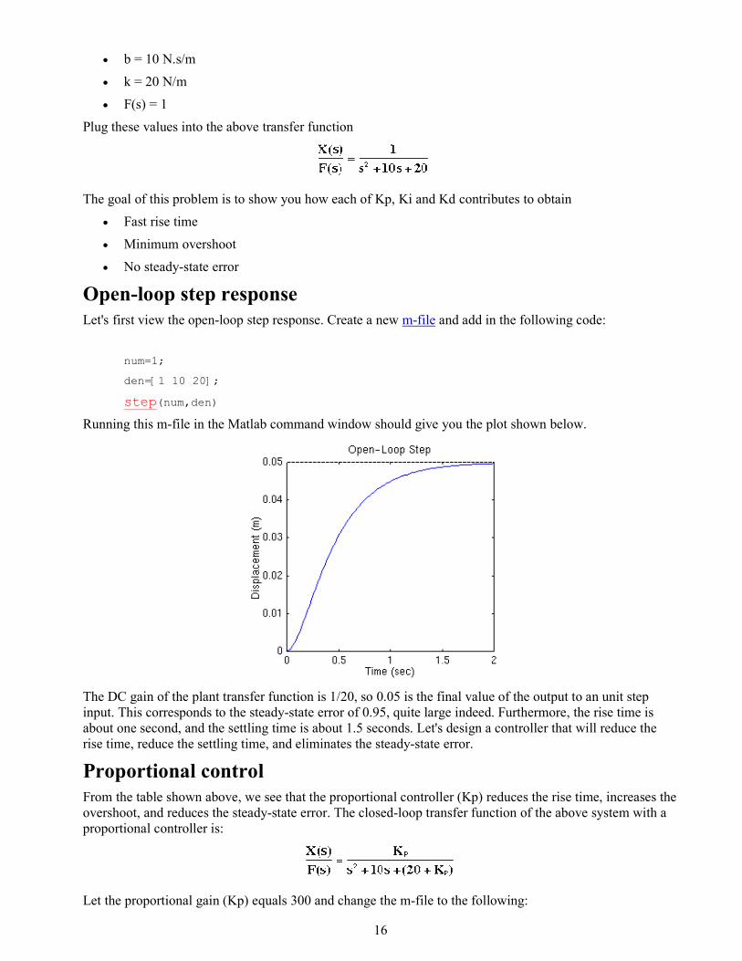
Open-loop step response

Let's first view the open-loop step response. Create a new m-file and add in the following code:

num=1;

den=[1 10 20];

step(num,den)

Running this m-file in the Matlab command window should give you the plot shown below.

The DC gain of the plant transfer function is 1/20, so 0.05 is the final value of the output to an unit step

input. This corresponds to the steady-state error of 0.95, quite large indeed. Furthermore, the rise time is

about one second, and the settling time is about 1.5 seconds. Let's design a controller that will reduce the

rise time, reduce the settling time, and eliminates the steady-state error.

Proportional control

From the table shown above, we see that the proportional controller (Kp) reduces the rise time, increases the

overshoot, and reduces the steady-state error. The closed-loop transfer function of the above system with a

proportional controller is:

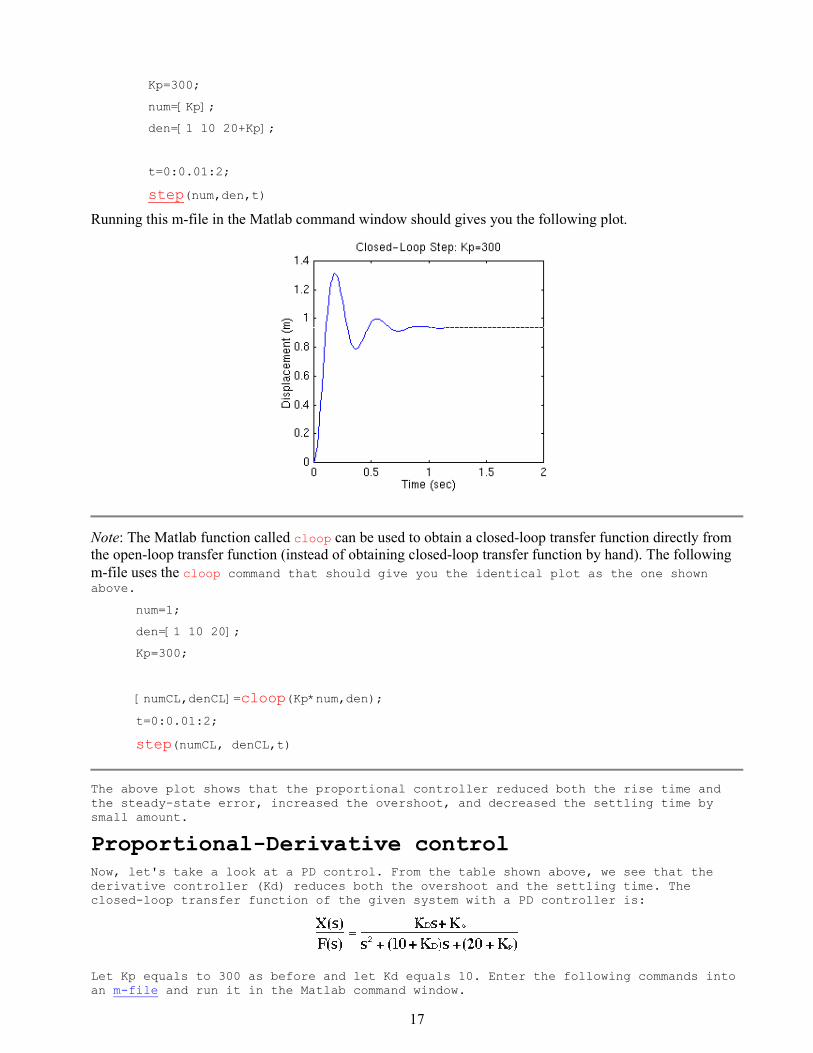
Let the proportional gain (Kp) equals 300 and change the m-file to the following:

17

Kp=300;

num=[Kp];

den=[1 10 20+Kp];

t=0:0.01:2;

step(num,den,t)

Running this m-file in the Matlab command window should gives you the following plot.

Note: The Matlab function called cloop can be used to obtain a closed-loop transfer function directly from

the open-loop transfer function (instead of obtaining closed-loop transfer function by hand). The following

m-file uses the cloop command that should give you the identical plot as the one shown above.

num=1;

den=[1 10 20];

Kp=300;

[numCL,denCL]=cloop(Kp*num,den);

t=0:0.01:2;

step(numCL, denCL,t)

The above plot shows that the proportional controller reduced both the rise time and

the steady-state error, increased the overshoot, and decreased the settling time by

small amount.

Proportional-Derivative control

Now, let's take a look at a PD control. From the table shown above, we see that the

derivative controller (Kd) reduces both the overshoot and the settling time. The

closed-loop transfer function of the given system with a PD controller is:

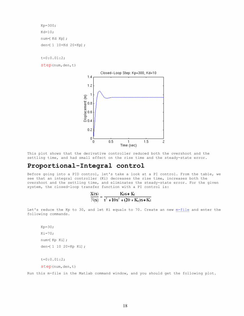
Let Kp equals to 300 as before and let Kd equals 10. Enter the following commands into

an m-file and run it in the Matlab command window.

18

Kp=300;

Kd=10;

num=[Kd Kp];

den=[1 10+Kd 20+Kp];

t=0:0.01:2;

step(num,den,t)

This plot shows that the derivative controller reduced both the overshoot and the

settling time, and had small effect on the rise time and the steady-state error.

Proportional-Integral control

Before going into a PID control, let's take a look at a PI control. From the table, we

see that an integral controller (Ki) decreases the rise time, increases both the

overshoot and the settling time, and eliminates the steady-state error. For the given

system, the closed-loop transfer function with a PI control is:

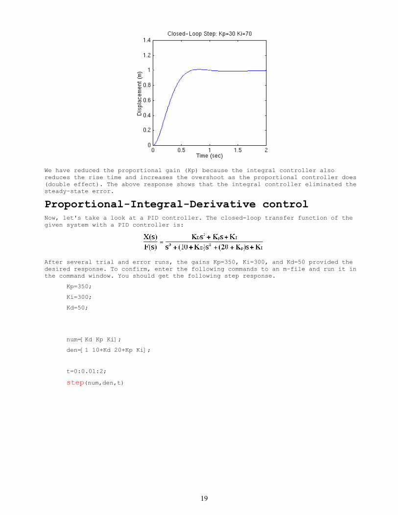
Let's reduce the Kp to 30, and let Ki equals to 70. Create an new m-file and enter the

following commands.

Kp=30;

Ki=70;

num=[Kp Ki];

den=[1 10 20+Kp Ki];

t=0:0.01:2;

step(num,den,t)

Run this m-file in the Matlab command window, and you should get the following plot.

19

We have reduced the proportional gain (Kp) because the integral controller also

reduces the rise time and increases the overshoot as the proportional controller does

(double effect). The above response shows that the integral controller eliminated the

steady-state error.

Proportional-Integral-Derivative control

Now, let's take a look at a PID controller. The closed-loop transfer function of the

given system with a PID controller is:

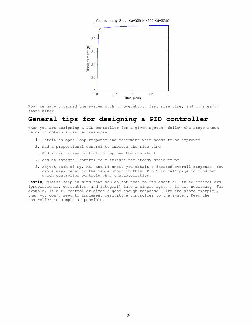
After several trial and error runs, the gains Kp=350, Ki=300, and Kd=50 provided the

desired response. To confirm, enter the following commands to an m-file and run it in

the command window. You should get the following step response.

Kp=350;

Ki=300;

Kd=50;

num=[Kd Kp Ki];

den=[1 10+Kd 20+Kp Ki];

t=0:0.01:2;

step(num,den,t)

20

Now, we have obtained the system with no overshoot, fast rise time, and no steady-

state error.

General tips for designing a PID controller

When you are designing a PID controller for a given system, follow the steps shown

below to obtain a desired response.

1. Obtain an open-loop response and determine what needs to be improved

2. Add a proportional control to improve the rise time

3. Add a derivative control to improve the overshoot

4. Add an integral control to eliminate the steady-state error

5. Adjust each of Kp, Ki, and Kd until you obtain a desired overall response. You

can always refer to the table shown in this "PID Tutorial" page to find out

which controller controls what characteristics.

Lastly, please keep in mind that you do not need to implement all three controllers

(proportional, derivative, and integral) into a single system, if not necessary. For

example, if a PI controller gives a good enough response (like the above example),

then you don't need to implement derivative controller to the system. Keep the

controller as simple as possible.

21

Root Locus Tutorial

Closed-loop poles

Plotting the root locus of a transfer function

Choosing a value of K from root locus

Closed-loop response

Key Matlab commands used in this tutorial: cloop, rlocfind, rlocus, sgrid, step

Matlab commands from the control system toolbox are highlighted in red.

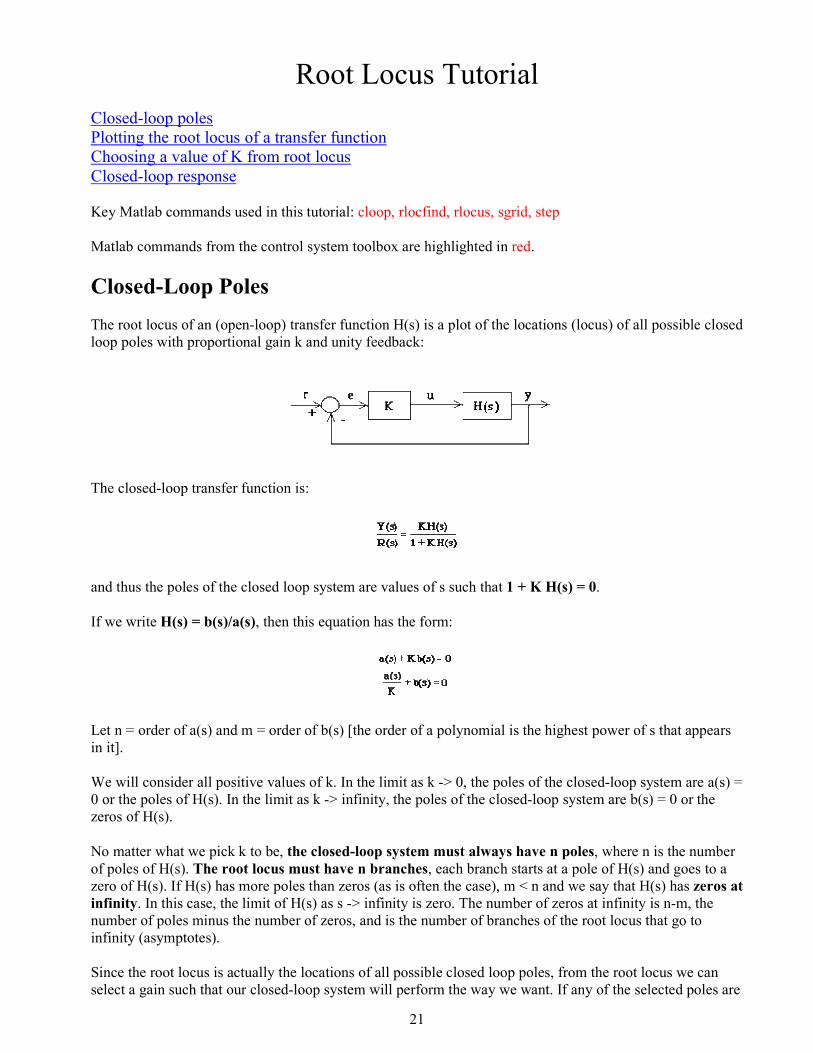
Closed-Loop Poles

The root locus of an (open-loop) transfer function H(s) is a plot of the locations (locus) of all possible closed

loop poles with proportional gain k and unity feedback:

The closed-loop transfer function is:

and thus the poles of the closed loop system are values of s such that 1 + K H(s) = 0.

If we write H(s) = b(s)/a(s), then this equation has the form:

Let n = order of a(s) and m = order of b(s) [the order of a polynomial is the highest power of s that appears

in it].

We will consider all positive values of k. In the limit as k -> 0, the poles of the closed-loop system are a(s) =

0 or the poles of H(s). In the limit as k -> infinity, the poles of the closed-loop system are b(s) = 0 or the

zeros of H(s).

No matter what we pick k to be, the closed-loop system must always have n poles, where n is the number

of poles of H(s). The root locus must have n branches, each branch starts at a pole of H(s) and goes to a

zero of H(s). If H(s) has more poles than zeros (as is often the case), m < n and we say that H(s) has zeros at

infinity. In this case, the limit of H(s) as s -> infinity is zero. The number of zeros at infinity is n-m, the

number of poles minus the number of zeros, and is the number of branches of the root locus that go to

infinity (asymptotes).

Since the root locus is actually the locations of all possible closed loop poles, from the root locus we can

select a gain such that our closed-loop system will perform the way we want. If any of the selected poles are

22

on the right half plane, the closed-loop system will be unstable. The poles that are closest to the imaginary

axis have the greatest influence on the closed-loop response, so even though the system has three or four

poles, it may still act like a second or even first order system depending on the location(s) of the dominant

pole(s).

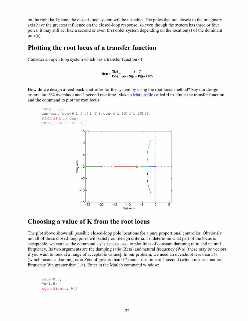
Plotting the root locus of a transfer function

Consider an open loop system which has a transfer function of

How do we design a feed-back controller for the system by using the root locus method? Say our design

criteria are 5% overshoot and 1 second rise time. Make a Matlab file called rl.m. Enter the transfer function,

and the command to plot the root locus:

num=[1 7];

den=conv(conv([1 0],[1 5]),conv([1 15],[1 20]));

rlocus(num,den) axis([-22 3 -15 15])

Choosing a value of K from the root locus

The plot above shows all possible closed-loop pole locations for a pure proportional controller. Obviously

not all of those closed-loop poles will satisfy our design criteria. To determine what part of the locus is

acceptable, we can use the command sgrid(Zeta,Wn) to plot lines of constant damping ratio and natural

frequency. Its two arguments are the damping ratio (Zeta) and natural frequency (Wn) [these may be vectors

if you want to look at a range of acceptable values]. In our problem, we need an overshoot less than 5%

(which means a damping ratio Zeta of greater than 0.7) and a rise time of 1 second (which means a natural

frequency Wn greater than 1.8). Enter in the Matlab command window:

zeta=0.7;

Wn=1.8;

sgrid(zeta, Wn)

23

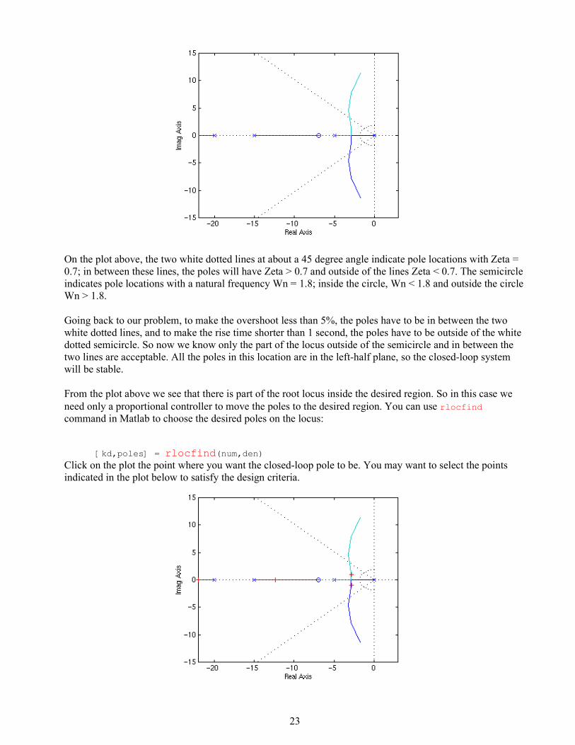
On the plot above, the two white dotted lines at about a 45 degree angle indicate pole locations with Zeta =

0.7; in between these lines, the poles will have Zeta > 0.7 and outside of the lines Zeta < 0.7. The semicircle

indicates pole locations with a natural frequency Wn = 1.8; inside the circle, Wn < 1.8 and outside the circle

Wn > 1.8.

Going back to our problem, to make the overshoot less than 5%, the poles have to be in between the two

white dotted lines, and to make the rise time shorter than 1 second, the poles have to be outside of the white

dotted semicircle. So now we know only the part of the locus outside of the semicircle and in between the

two lines are acceptable. All the poles in this location are in the left-half plane, so the closed-loop system

will be stable.

From the plot above we see that there is part of the root locus inside the desired region. So in this case we

need only a proportional controller to move the poles to the desired region. You can use rlocfind

command in Matlab to choose the desired poles on the locus:

[kd,poles] = rlocfind(num,den)

Click on the plot the point where you want the closed-loop pole to be. You may want to select the points

indicated in the plot below to satisfy the design criteria.

24

Note that since the root locus may has more than one branch, when you select a pole, you may want to find

out where the other pole (poles) are. Remember they will affect the response too. From the plot above we

see that all the poles selected (all the white "+") are at reasonable positions. We can go ahead and use the

chosen kd as our proportional controller.

Closed-loop response

In order to find the step response, you need to know the closed-loop transfer function. You could compute

this using the rules of block diagrams, or let Matlab do it for you:

[numCL, denCL] = cloop((kd)*num, den)

The two arguments to the function cloop are the numerator and denominator of the open-loop system. You

need to include the proportional gain that you have chosen. Unity feedback is assumed.

If you have a non-unity feedback situation, look at the help file for the Matlab function feedback,

which can find the closed-loop transfer function with a gain in the feedback loop.

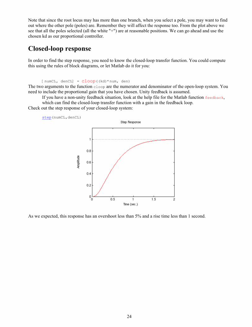
Check out the step response of your closed-loop system:

step(numCL,denCL)

As we expected, this response has an overshoot less than 5% and a rise time less than 1 second.

25

Frequency Response Analysis and Design Tutorial

I. Bode plots [ Gain and phase margin | Bandwidth frequency | Closed loop response ]

II. The Nyquist diagram [ Closed loop stability | Gain margin | Phase margin ]

Key matlab commands used in these tutorial are bode, nyquist, nyquist1, lnyquist1, margin, lsim, step, and

cloop

The frequency response method may be less intuitive than other methods you have studied previously.

However, it has certain advantages, especially in real-life situations such as modeling transfer functions

from physical data.

The frequency response of a system can be viewed two different ways: via the Bode plot or via the Nyquist

diagram. Both methods display the same information; the difference lies in the way the information is

presented. We will study both methods in this tutorial.

The frequency response is a representation of the system's response to sinusoidal inputs at varying

frequencies. The output of a linear system to a sinusoidal input is a sinusoid of the same frequency but with

a different magnitude and phase. The frequency response is defined as the magnitude and phase differences

between the input and output sinusoids. In this tutorial, we will see how we can use the open-loop frequency

response of a system to predict its behavior in closed-loop.

To plot the frequency response, we create a vector of frequencies (varying between zero or "DC" and

infinity) and compute the value of the plant transfer function at those frequencies. If G(s) is the open loop

transfer function of a system and w is the frequency vector, we then plot G(j*w) vs. w. Since G(j*w) is a

complex number, we can plot both its magnitude and phase (the Bode plot) or its position in the complex

plane (the Nyquist plot). More information is available on plotting the frequency response.

Bode Plots

As noted above, a Bode plot is the representation of the magnitude and phase of G(j*w) (where the

frequency vector w contains only positive frequencies). To see the Bode plot of a transfer function, you can

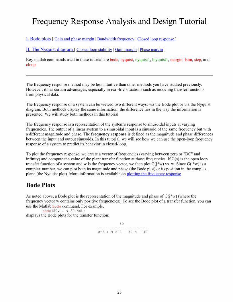
use the Matlab bode command. For example, bode(50,[1 9 30 40])

displays the Bode plots for the transfer function:

50

-----------------------

s^3 + 9 s^2 + 30 s + 40

26

Please note the axes of the figure. The frequency is on a logarithmic scale, the phase is given in degrees, and

the magnitude is given as the gain in decibels.

Note: a decibel is defined as 20*log10 ( |G(j*w| )

Click here to see a few simple Bode plots.

Gain and Phase Margin

Let's say that we have the following system:

where K is a variable (constant) gain and G(s) is the plant under consideration. The gain margin is defined

as the change in open loop gain required to make the system unstable. Systems with greater gain margins

can withstand greater changes in system parameters before becoming unstable in closed loop.

Keep in mind that unity gain in magnitude is equal to a gain of zero in dB.

The phase margin is defined as the change in open loop phase shift required to make a closed loop system

unstable.

The phase margin also measures the system's tolerance to time delay. If there is a time delay greater than

180/Wpc in the loop (where Wpc is the frequency where the phase shift is 180 deg), the system will become

unstable in closed loop. The time delay can be thought of as an extra block in the forward path of the block

diagram that adds phase to the system but has no effect the gain. That is, a time delay can be represented as

a block with magnitude of 1 and phase w*time_delay (in radians/second).

For now, we won't worry about where all this comes from and will concentrate on identifying the gain and

phase margins on a Bode plot:

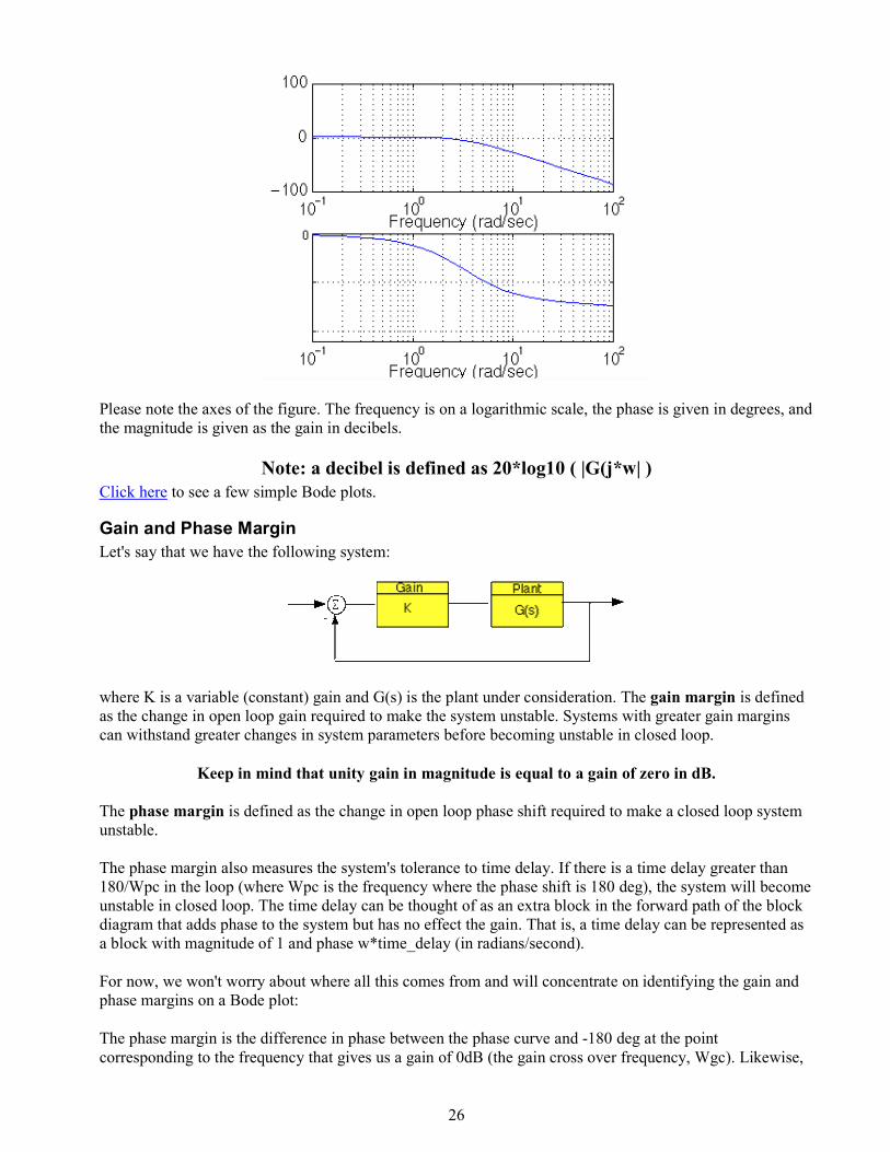
The phase margin is the difference in phase between the phase curve and -180 deg at the point

corresponding to the frequency that gives us a gain of 0dB (the gain cross over frequency, Wgc). Likewise,

27

the gain margin is the difference between the magnitude curve and 0dB at the point corresponding to the

frequency that gives us a phase of -180 deg (the phase cross over frequency, Wpc).

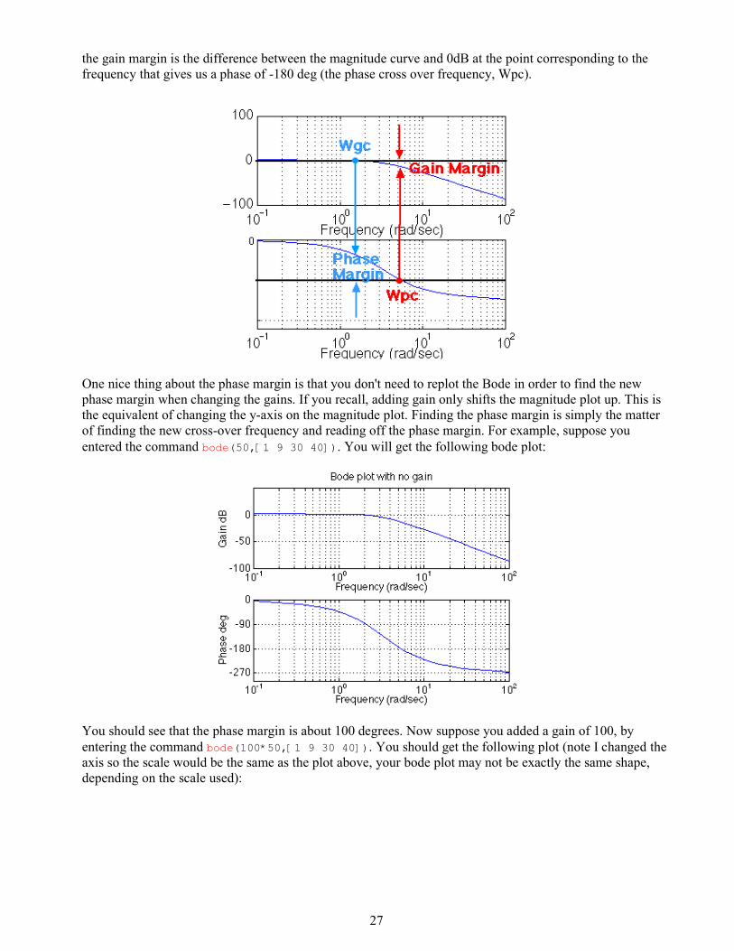
One nice thing about the phase margin is that you don't need to replot the Bode in order to find the new

phase margin when changing the gains. If you recall, adding gain only shifts the magnitude plot up. This is

the equivalent of changing the y-axis on the magnitude plot. Finding the phase margin is simply the matter

of finding the new cross-over frequency and reading off the phase margin. For example, suppose you

entered the command bode(50,[1 9 30 40]). You will get the following bode plot:

You should see that the phase margin is about 100 degrees. Now suppose you added a gain of 100, by

entering the command bode(100*50,[1 9 30 40]). You should get the following plot (note I changed the

axis so the scale would be the same as the plot above, your bode plot may not be exactly the same shape,

depending on the scale used):

28

As you can see the phase plot is exactly the same as before, and the magnitude plot is shifted up by 40dB

(gain of 100). The phase margin is now about -60 degrees. This same result could be achieved if the y-axis

of the magnitude plot was shifted down 40dB. Try this, look at the first Bode plot, find where the curve

crosses the -40dB line, and read off the phase margin. It should be about -60 degrees, the same as the second

Bode plot.

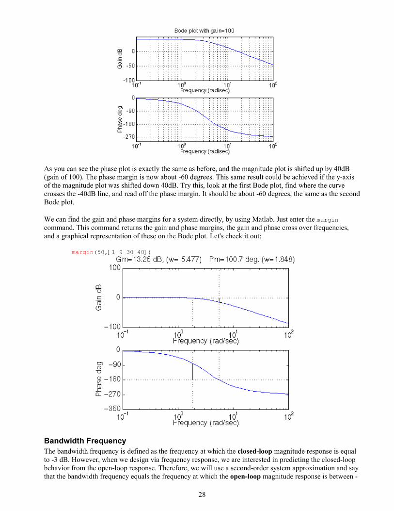
We can find the gain and phase margins for a system directly, by using Matlab. Just enter the margin

command. This command returns the gain and phase margins, the gain and phase cross over frequencies,

and a graphical representation of these on the Bode plot. Let's check it out:

margin(50,[1 9 30 40])

Bandwidth Frequency

The bandwidth frequency is defined as the frequency at which the closed-loop magnitude response is equal

to -3 dB. However, when we design via frequency response, we are interested in predicting the closed-loop

behavior from the open-loop response. Therefore, we will use a second-order system approximation and say

that the bandwidth frequency equals the frequency at which the open-loop magnitude response is between -

29

6 and - 7.5dB, assuming the open loop phase response is between -135 deg and -225 deg. For a complete

derivation of this approximation, consult your textbook.

If you would like to see how the bandwidth of a system can be found mathematically from the closed-loop

damping ratio and natural frequency, the relevant equations as well as some plots and Matlab code are given

on our Bandwidth Frequency page.

In order to illustrate the importance of the bandwidth frequency, we will show how the output changes with

different input frequencies. We will find that sinusoidal inputs with frequency less than Wbw (the

bandwidth frequency) are tracked "reasonably well" by the system. Sinusoidal inputs with frequency greater

than Wbw are attenuated (in magnitude) by a factor of 0.707 or greater (and are also shifted in phase).

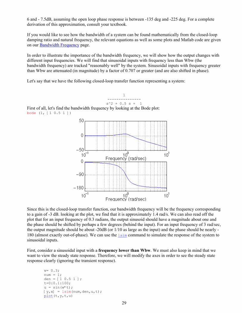
Let's say that we have the following closed-loop transfer function representing a system:

1

---------------

s^2 + 0.5 s + 1

First of all, let's find the bandwidth frequency by looking at the Bode plot: bode (1, [1 0.5 1 ])

Since this is the closed-loop transfer function, our bandwidth frequency will be the frequency corresponding

to a gain of -3 dB. looking at the plot, we find that it is approximately 1.4 rad/s. We can also read off the

plot that for an input frequency of 0.3 radians, the output sinusoid should have a magnitude about one and

the phase should be shifted by perhaps a few degrees (behind the input). For an input frequency of 3 rad/sec,

the output magnitude should be about -20dB (or 1/10 as large as the input) and the phase should be nearly -

180 (almost exactly out-of-phase). We can use the lsim command to simulate the response of the system to

sinusoidal inputs.

First, consider a sinusoidal input with a frequency lower than Wbw. We must also keep in mind that we

want to view the steady state response. Therefore, we will modify the axes in order to see the steady state

response clearly (ignoring the transient response).

w= 0.3;

num = 1;

den = [1 0.5 1 ];

t=0:0.1:100;

u = sin(w*t);

[y,x] = lsim(num,den,u,t);

plot(t,y,t,u)

30

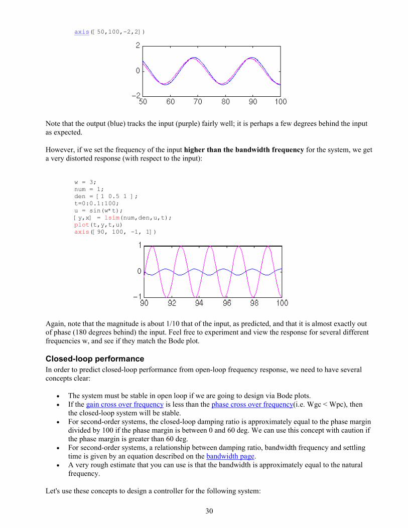
axis([50,100,-2,2])

Note that the output (blue) tracks the input (purple) fairly well; it is perhaps a few degrees behind the input

as expected.

However, if we set the frequency of the input higher than the bandwidth frequency for the system, we get

a very distorted response (with respect to the input):

w = 3;

num = 1;

den = [1 0.5 1 ];

t=0:0.1:100;

u = sin(w*t);

[y,x] = lsim(num,den,u,t);

plot(t,y,t,u)

axis([90, 100, -1, 1])

Again, note that the magnitude is about 1/10 that of the input, as predicted, and that it is almost exactly out

of phase (180 degrees behind) the input. Feel free to experiment and view the response for several different

frequencies w, and see if they match the Bode plot.

Closed-loop performance

In order to predict closed-loop performance from open-loop frequency response, we need to have several

concepts clear:

• The system must be stable in open loop if we are going to design via Bode plots.

• If the gain cross over frequency is less than the phase cross over frequency(i.e. Wgc < Wpc), then

the closed-loop system will be stable.

• For second-order systems, the closed-loop damping ratio is approximately equal to the phase margin

divided by 100 if the phase margin is between 0 and 60 deg. We can use this concept with caution if

the phase margin is greater than 60 deg.

• For second-order systems, a relationship between damping ratio, bandwidth frequency and settling

time is given by an equation described on the bandwidth page.

• A very rough estimate that you can use is that the bandwidth is approximately equal to the natural

frequency.

Let's use these concepts to design a controller for the following system:

31

Where Gc(s) is the controller and G(s) is:

10

----------

1.25s + 1

The design must meet the following specifications:

• Zero steady state error.

• Maximum overshoot must be less than 40%.

• Settling time must be less than 2 secs.

There are two ways of solving this problem: one is graphical and the other is numerical. Within Matlab, the

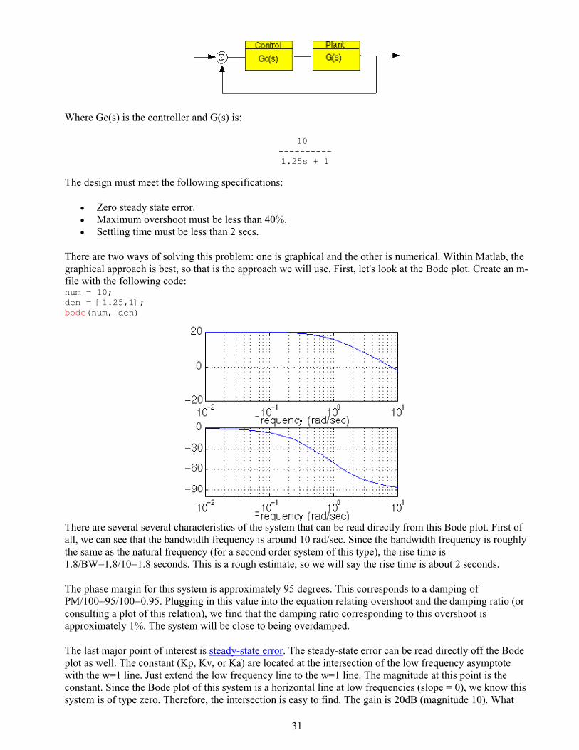
graphical approach is best, so that is the approach we will use. First, let's look at the Bode plot. Create an m-

file with the following code: num = 10;

den = [1.25,1];

bode(num, den)

There are several several characteristics of the system that can be read directly from this Bode plot. First of

all, we can see that the bandwidth frequency is around 10 rad/sec. Since the bandwidth frequency is roughly

the same as the natural frequency (for a second order system of this type), the rise time is

1.8/BW=1.8/10=1.8 seconds. This is a rough estimate, so we will say the rise time is about 2 seconds.

The phase margin for this system is approximately 95 degrees. This corresponds to a damping of

PM/100=95/100=0.95. Plugging in this value into the equation relating overshoot and the damping ratio (or

consulting a plot of this relation), we find that the damping ratio corresponding to this overshoot is

approximately 1%. The system will be close to being overdamped.

The last major point of interest is steady-state error. The steady-state error can be read directly off the Bode

plot as well. The constant (Kp, Kv, or Ka) are located at the intersection of the low frequency asymptote

with the w=1 line. Just extend the low frequency line to the w=1 line. The magnitude at this point is the

constant. Since the Bode plot of this system is a horizontal line at low frequencies (slope = 0), we know this

system is of type zero. Therefore, the intersection is easy to find. The gain is 20dB (magnitude 10). What

32

this means is that the constant for the error function it 10. Click here to see the table of system types and

error functions. The steady-state error is 1/(1+Kp)=1/(1+10)=0.091. If our system was type one instead of

type zero, the constant for the steady-state error would be found in a manner similar to the following

Let's check our predictions by looking at a step response plot. This can be done by adding the following two

lines of code into the Matlab command window.

[numc,denc] = cloop(num,den,-1);

step(numc,denc)

As you can see, our predictions were very good. The system has a rise time of about 2 seconds, is

overdamped, and has a steady-state error of about 9%. Now we need to choose a controller that will allow

us to meet the design criteria. We choose a PI controller because it will yield zero steady state error for a

step input. Also, the PI controller has a zero, which we can place. This gives us additional design flexibility

to help us meet our criteria. Recall that a PI controller is given by:

K*(s+a)

Gc(s) = -------

s

The first thing we need to find is the damping ratio corresponding to a percent overshoot of 40%. Plugging

in this value into the equation relating overshoot and damping ratio (or consulting a plot of this relation), we

find that the damping ratio corresponding to this overshoot is approximately 0.28. Therefore, our phase

margin should be approximately 30 degrees. From our Ts*Wbw vs damping ratio plot, we find that

Ts*Wbw ~ 21. We must have a bandwidth frequency greater than or equal to 12 if we want our settling time

to be less than 1.75 seconds which meets the design specs.

33

Now that we know our desired phase margin and bandwidth frequency, we can start our design. Remember

that we are looking at the open-loop Bode plots. Therefore, our bandwidth frequency will be the frequency

corresponding to a gain of approximately -7 dB.

Let's see how the integrator portion of the PI or affects our response. Change your m-file to look like the

following (this adds an integral term but no proportional term):

num = [10];

den = [1.25, 1];

numPI = [1];

denPI = [1 0];

newnum = conv(num,numPI);

newden = conv(den,denPI);

bode(newnum, newden, logspace(0,2))

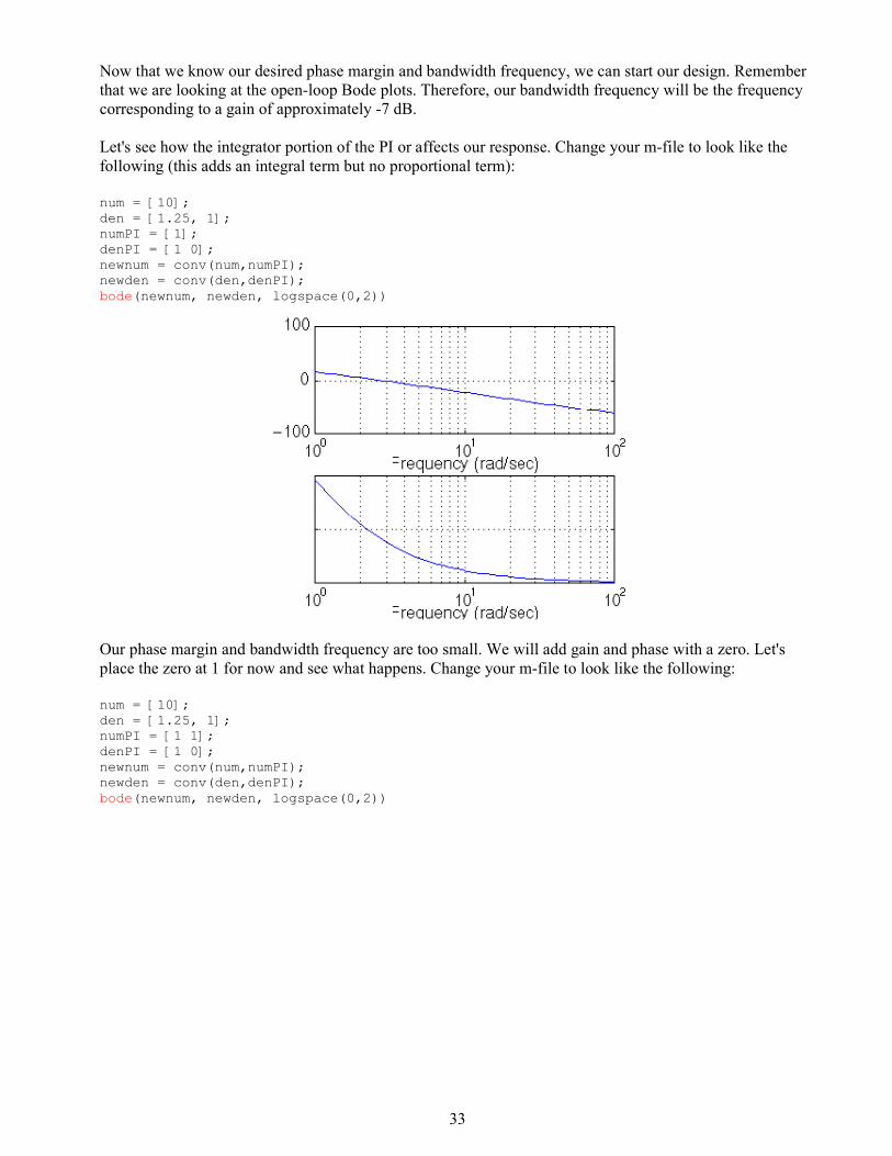
Our phase margin and bandwidth frequency are too small. We will add gain and phase with a zero. Let's

place the zero at 1 for now and see what happens. Change your m-file to look like the following:

num = [10];

den = [1.25, 1];

numPI = [1 1];

denPI = [1 0];

newnum = conv(num,numPI);

newden = conv(den,denPI);

bode(newnum, newden, logspace(0,2))

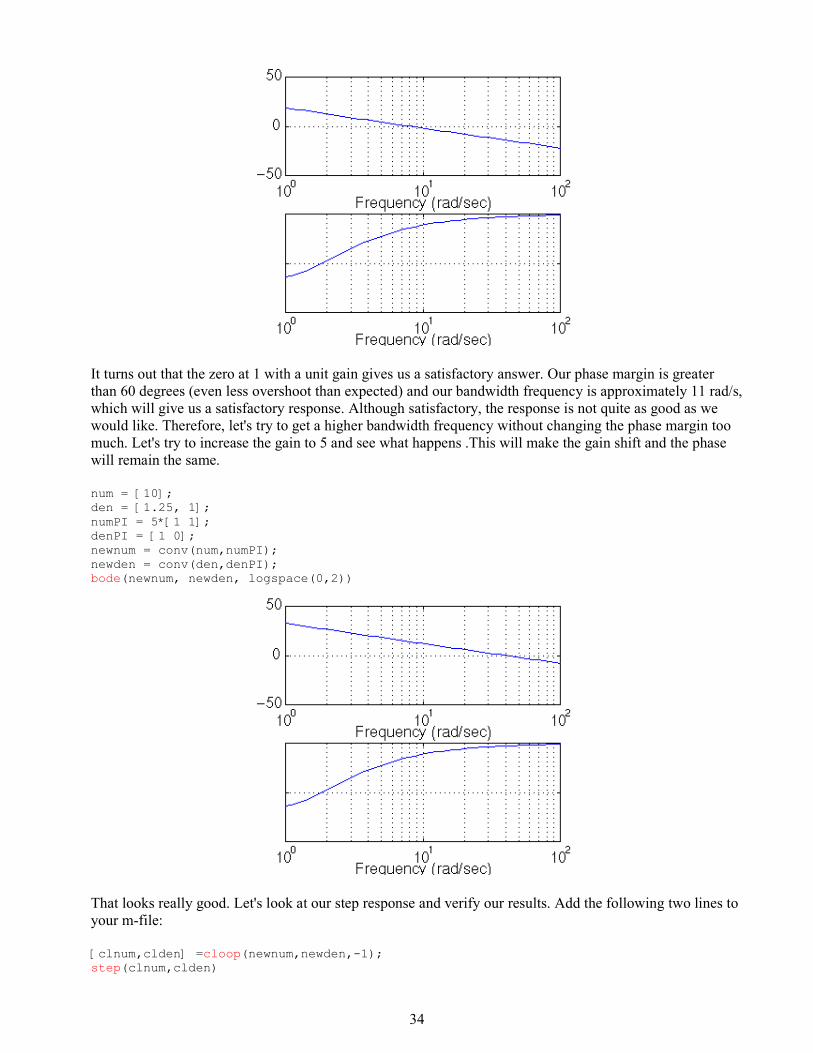
34

It turns out that the zero at 1 with a unit gain gives us a satisfactory answer. Our phase margin is greater

than 60 degrees (even less overshoot than expected) and our bandwidth frequency is approximately 11 rad/s,

which will give us a satisfactory response. Although satisfactory, the response is not quite as good as we

would like. Therefore, let's try to get a higher bandwidth frequency without changing the phase margin too

much. Let's try to increase the gain to 5 and see what happens .This will make the gain shift and the phase

will remain the same.

num = [10];

den = [1.25, 1];

numPI = 5*[1 1];

denPI = [1 0];

newnum = conv(num,numPI);

newden = conv(den,denPI);

bode(newnum, newden, logspace(0,2))

That looks really good. Let's look at our step response and verify our results. Add the following two lines to

your m-file:

[clnum,clden] =cloop(newnum,newden,-1);

step(clnum,clden)

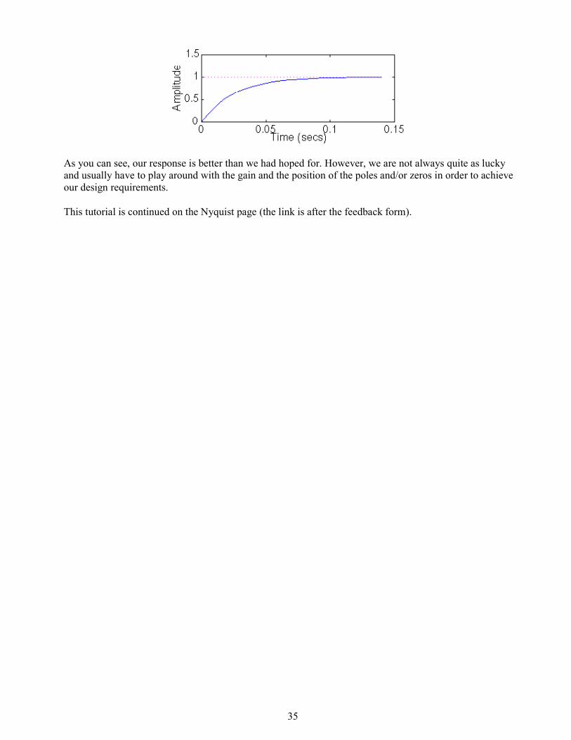
35

As you can see, our response is better than we had hoped for. However, we are not always quite as lucky

and usually have to play around with the gain and the position of the poles and/or zeros in order to achieve

our design requirements.

This tutorial is continued on the Nyquist page (the link is after the feedback form).

36

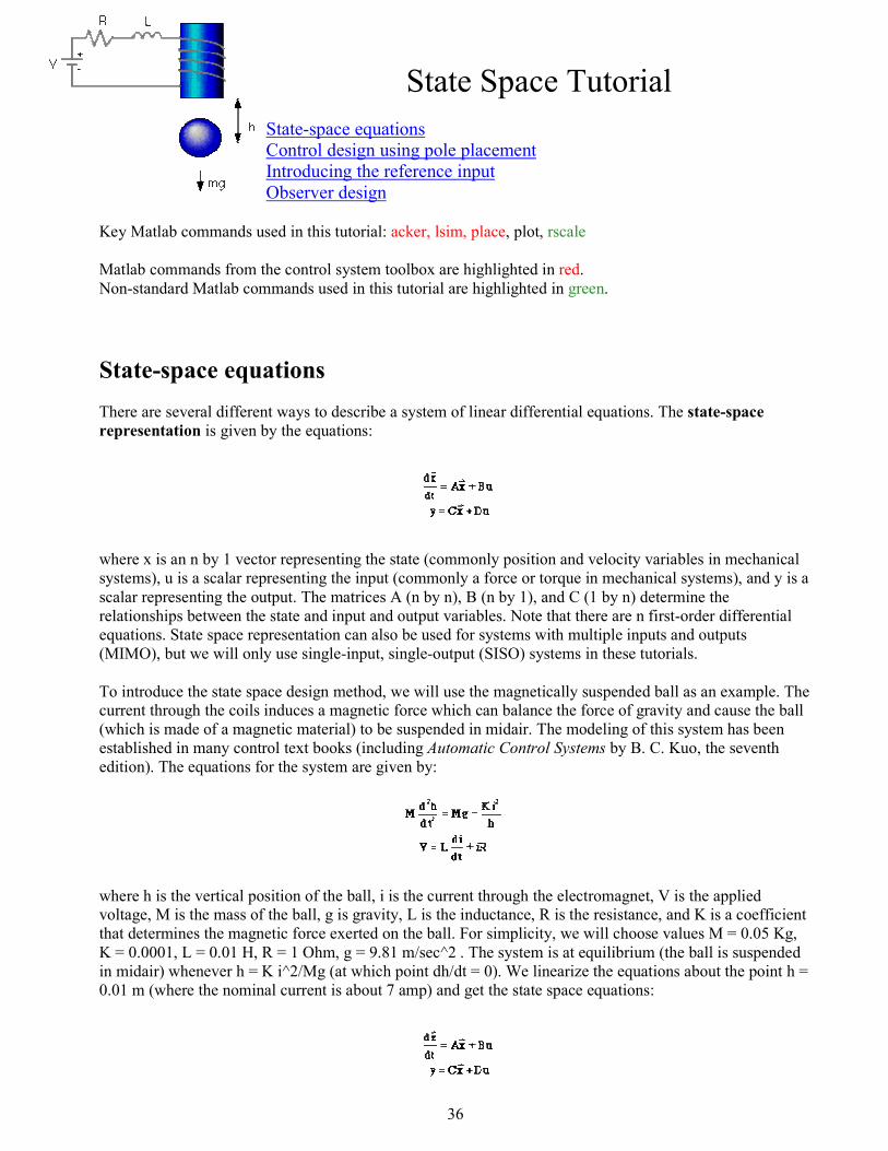
State Space Tutorial

State-space equations

Control design using pole placement

Introducing the reference input

Observer design

Key Matlab commands used in this tutorial: acker, lsim, place, plot, rscale

Matlab commands from the control system toolbox are highlighted in red.

Non-standard Matlab commands used in this tutorial are highlighted in green.

State-space equations

There are several different ways to describe a system of linear differential equations. The state-space

representation is given by the equations:

where x is an n by 1 vector representing the state (commonly position and velocity variables in mechanical

systems), u is a scalar representing the input (commonly a force or torque in mechanical systems), and y is a

scalar representing the output. The matrices A (n by n), B (n by 1), and C (1 by n) determine the

relationships between the state and input and output variables. Note that there are n first-order differential

equations. State space representation can also be used for systems with multiple inputs and outputs

(MIMO), but we will only use single-input, single-output (SISO) systems in these tutorials.

To introduce the state space design method, we will use the magnetically suspended ball as an example. The

current through the coils induces a magnetic force which can balance the force of gravity and cause the ball

(which is made of a magnetic material) to be suspended in midair. The modeling of this system has been

established in many control text books (including Automatic Control Systems by B. C. Kuo, the seventh

edition). The equations for the system are given by:

where h is the vertical position of the ball, i is the current through the electromagnet, V is the applied

voltage, M is the mass of the ball, g is gravity, L is the inductance, R is the resistance, and K is a coefficient

that determines the magnetic force exerted on the ball. For simplicity, we will choose values M = 0.05 Kg,

K = 0.0001, L = 0.01 H, R = 1 Ohm, g = 9.81 m/sec^2 . The system is at equilibrium (the ball is suspended

in midair) whenever h = K i^2/Mg (at which point dh/dt = 0). We linearize the equations about the point h =

0.01 m (where the nominal current is about 7 amp) and get the state space equations:

37

where: is the set of state variables for the system (a 3x1 vector), u is the input voltage (delta V), and

y (the output), is delta h. Enter the system matrices into a m-file. A = [ 0 1 0

980 0 -2.8

0 0 -100];

B = [0

0

100];

C = [1 0 0];

One of the first things you want to do with the state equations is find the poles of the system; these are the

values of s where det(sI - A) = 0, or the eigenvalues of the A matrix:

poles = eig(A)

You should get the following three poles: poles =

31.3050

-31.3050

-100.0000

One of the poles is in the right-half plane, which means that the system is unstable in open-loop.

To check out what happens to this unstable system when there is a nonzero initial condition, add the

following lines to your m-file,

t = 0:0.01:2;

u = 0*t;

x0 = [0.005 0 0];

[y,x] = lsim(A,B,C,0,u,t,x0);

h = x(:,2); %Delta-h is the output of interest

plot(t,h)

and run the file again.

It looks like the distance between the ball and the electromagnet will go to infinity, but probably the ball hits

the table or the floor first (and also probably goes out of the range where our linearization is valid).

Control design using pole placement

38

Let's build a controller for this system. The schematic of a full-state feedback system is the following:

Recall that the characteristic polynomial for this closed-loop system is the determinant of (sI-(A-BK)).

Since the matrices A and B*K are both 3 by 3 matrices, there will be 3 Wpoles for the system. By using full-

state feedback we can place the poles anywhere we want. We could use the Matlab function place to find

the control matrix, K, which will give the desired poles.

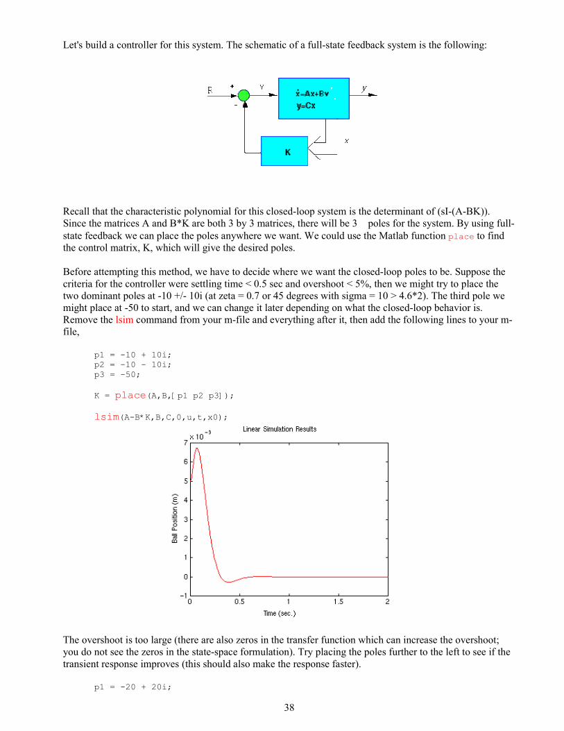
Before attempting this method, we have to decide where we want the closed-loop poles to be. Suppose the

criteria for the controller were settling time < 0.5 sec and overshoot < 5%, then we might try to place the

two dominant poles at -10 +/- 10i (at zeta = 0.7 or 45 degrees with sigma = 10 > 4.6*2). The third pole we

might place at -50 to start, and we can change it later depending on what the closed-loop behavior is.

Remove the lsim command from your m-file and everything after it, then add the following lines to your m-

file,

p1 = -10 + 10i;

p2 = -10 - 10i;

p3 = -50;

K = place(A,B,[p1 p2 p3]);

lsim(A-B*K,B,C,0,u,t,x0);

The overshoot is too large (there are also zeros in the transfer function which can increase the overshoot;

you do not see the zeros in the state-space formulation). Try placing the poles further to the left to see if the

transient response improves (this should also make the response faster).

p1 = -20 + 20i;

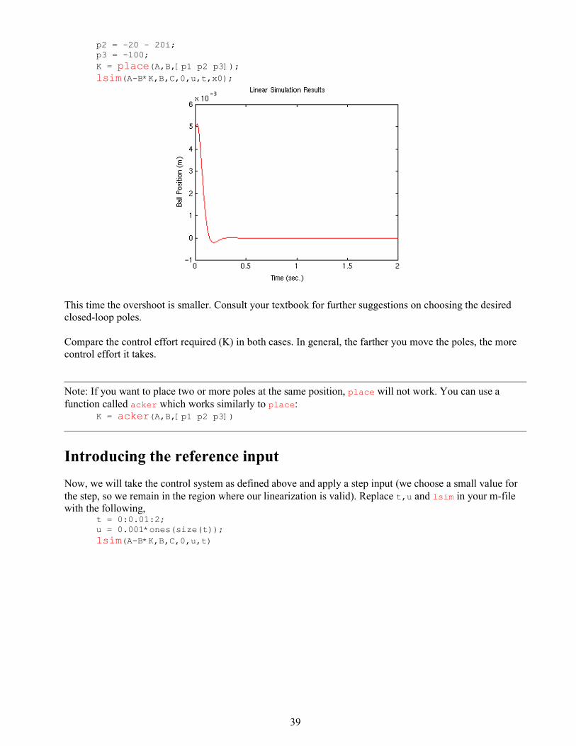
39

p2 = -20 - 20i;

p3 = -100;

K = place(A,B,[p1 p2 p3]);

lsim(A-B*K,B,C,0,u,t,x0);

This time the overshoot is smaller. Consult your textbook for further suggestions on choosing the desired

closed-loop poles.

Compare the control effort required (K) in both cases. In general, the farther you move the poles, the more

control effort it takes.

Note: If you want to place two or more poles at the same position, place will not work. You can use a

function called acker which works similarly to place: K = acker(A,B,[p1 p2 p3])

Introducing the reference input

Now, we will take the control system as defined above and apply a step input (we choose a small value for

the step, so we remain in the region where our linearization is valid). Replace t,u and lsim in your m-file

with the following, t = 0:0.01:2;

u = 0.001*ones(size(t));

lsim(A-B*K,B,C,0,u,t)

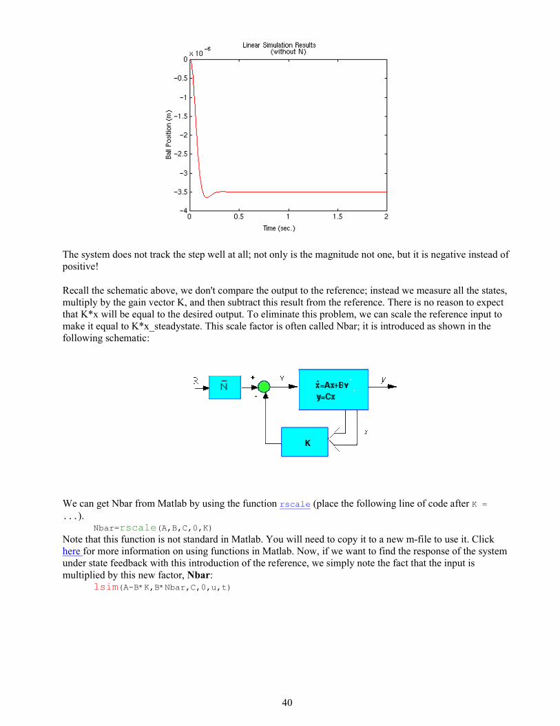
40

The system does not track the step well at all; not only is the magnitude not one, but it is negative instead of

positive!

Recall the schematic above, we don't compare the output to the reference; instead we measure all the states,

multiply by the gain vector K, and then subtract this result from the reference. There is no reason to expect

that K*x will be equal to the desired output. To eliminate this problem, we can scale the reference input to

make it equal to K*x_steadystate. This scale factor is often called Nbar; it is introduced as shown in the

following schematic:

We can get Nbar from Matlab by using the function rscale (place the following line of code after K =

...). Nbar=rscale(A,B,C,0,K)

Note that this function is not standard in Matlab. You will need to copy it to a new m-file to use it. Click

here for more information on using functions in Matlab. Now, if we want to find the response of the system

under state feedback with this introduction of the reference, we simply note the fact that the input is

multiplied by this new factor, Nbar: lsim(A-B*K,B*Nbar,C,0,u,t)

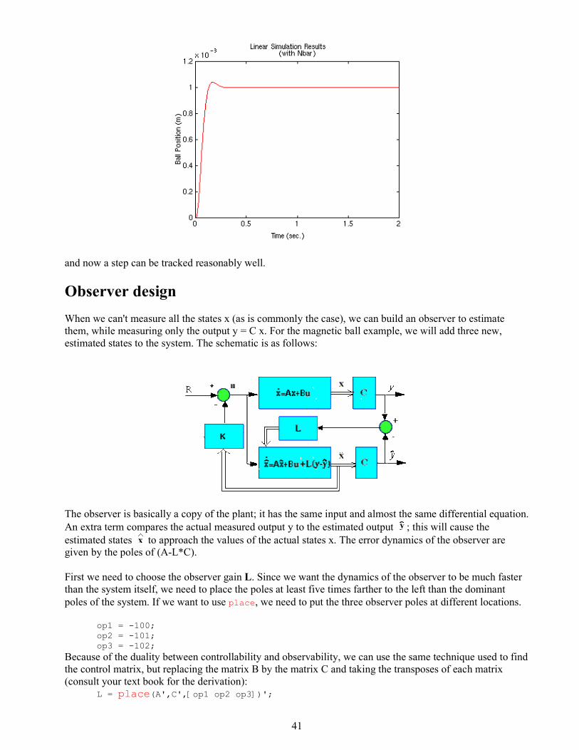
41

and now a step can be tracked reasonably well.

Observer design

When we can't measure all the states x (as is commonly the case), we can build an observer to estimate

them, while measuring only the output y = C x. For the magnetic ball example, we will add three new,

estimated states to the system. The schematic is as follows:

The observer is basically a copy of the plant; it has the same input and almost the same differential equation.

An extra term compares the actual measured output y to the estimated output ; this will cause the

estimated states to approach the values of the actual states x. The error dynamics of the observer are

given by the poles of (A-L*C).

First we need to choose the observer gain L. Since we want the dynamics of the observer to be much faster

than the system itself, we need to place the poles at least five times farther to the left than the dominant

poles of the system. If we want to use place, we need to put the three observer poles at different locations.

op1 = -100;

op2 = -101;

op3 = -102;

Because of the duality between controllability and observability, we can use the same technique used to find

the control matrix, but replacing the matrix B by the matrix C and taking the transposes of each matrix

(consult your text book for the derivation): L = place(A',C',[op1 op2 op3])';

42

The equations in the block diagram above are given for . It is conventional to write the combined

equations for the system plus observer using the original state x plus the error state: e = x - . We use as

state feedback u = -K . After a little bit of algebra (consult your textbook for more details), we arrive at

the combined state and error equations with the full-state feedback and an observer: At = [A - B*K B*K

zeros(size(A)) A - L*C];

Bt = [ B*Nbar

zeros(size(B))];

Ct = [ C zeros(size(C))];

To see how the response looks to a nonzero initial condition with no reference input, add the following lines

into your m-file. We typically assume that the observer begins with zero initial condition, =0. This gives

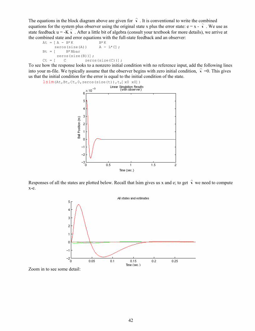
us that the initial condition for the error is equal to the initial condition of the state. lsim(At,Bt,Ct,0,zeros(size(t)),t,[x0 x0])

Responses of all the states are plotted below. Recall that lsim gives us x and e; to get we need to compute

x-e.

Zoom in to see some detail:

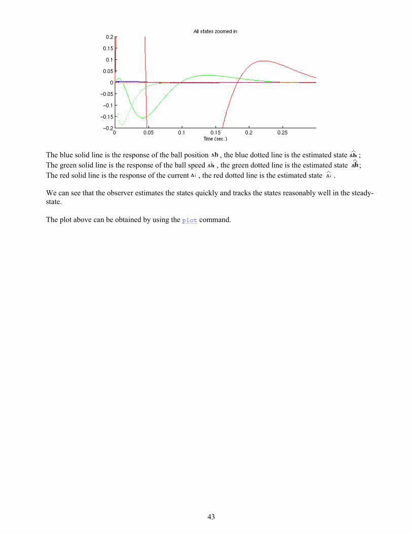
43

The blue solid line is the response of the ball position , the blue dotted line is the estimated state ;

The green solid line is the response of the ball speed , the green dotted line is the estimated state ;

The red solid line is the response of the current , the red dotted line is the estimated state .

We can see that the observer estimates the states quickly and tracks the states reasonably well in the steady-

state.

The plot above can be obtained by using the plot command.

44

Digital Control Tutorial

Introduction

Zero-order hold equivalence

Conversion using c2dm

Stability and transient response

Discrete Root-Locus

Key Matlab Commands used in this tutorial are: c2dm pzmap zgrid dstep stairs rlocus

Note: Matlab commands from the control system toolbox are highlighted in red.

Introduction

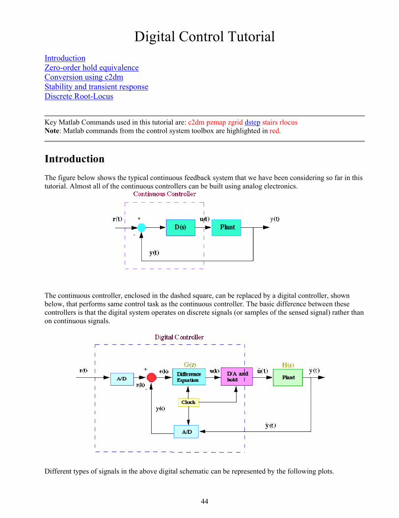
The figure below shows the typical continuous feedback system that we have been considering so far in this

tutorial. Almost all of the continuous controllers can be built using analog electronics.

The continuous controller, enclosed in the dashed square, can be replaced by a digital controller, shown

below, that performs same control task as the continuous controller. The basic difference between these

controllers is that the digital system operates on discrete signals (or samples of the sensed signal) rather than

on continuous signals.

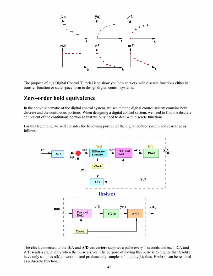
Different types of signals in the above digital schematic can be represented by the following plots.

45

The purpose of this Digital Control Tutorial is to show you how to work with discrete functions either in

transfer function or state-space form to design digital control systems.

Zero-order hold equivalence

In the above schematic of the digital control system, we see that the digital control system contains both

discrete and the continuous portions. When designing a digital control system, we need to find the discrete

equivalent of the continuous portion so that we only need to deal with discrete functions.

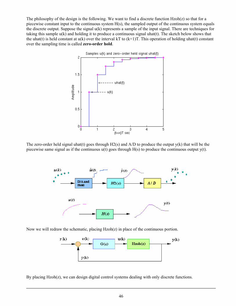
For this technique, we will consider the following portion of the digital control system and rearrange as

follows.

The clock connected to the D/A and A/D converters supplies a pulse every T seconds and each D/A and

A/D sends a signal only when the pulse arrives. The purpose of having this pulse is to require that Hzoh(z)

have only samples u(k) to work on and produce only samples of output y(k); thus, Hzoh(z) can be realized

as a discrete function.

46

The philosophy of the design is the following. We want to find a discrete function Hzoh(z) so that for a

piecewise constant input to the continuous system H(s), the sampled output of the continuous system equals

the discrete output. Suppose the signal u(k) represents a sample of the input signal. There are techniques for

taking this sample u(k) and holding it to produce a continuous signal uhat(t). The sketch below shows that

the uhat(t) is held constant at u(k) over the interval kT to (k+1)T. This operation of holding uhat(t) constant

over the sampling time is called zero-order hold.

The zero-order held signal uhat(t) goes through H2(s) and A/D to produce the output y(k) that will be the

piecewise same signal as if the continuous u(t) goes through H(s) to produce the continuous output y(t).

Now we will redraw the schematic, placing Hzoh(z) in place of the continuous portion.

By placing Hzoh(z), we can design digital control systems dealing with only discrete functions.

47

Note: There are certain cases where the discrete response does not match the continuous response due to a

hold circuit implemented in digital control systems. For information, see Lagging effect associated with the

hold.

Conversion using c2dm

There is a Matlab function called c2dm that converts a given continuous system (either in transfer function

or state-space form) to discrete system using the zero-order hold operation explained above. The basic

command for this c2dm is one of the following.

[numDz,denDz] = c2dm (num,den,Ts,'zoh')

[F,G,H,J] = c2dm (A,B,C,D,Ts,'zoh')

The sampling time (Ts in sec/sample) should be smaller than 1/(30*BW), where BW is the closed-loop

bandwidth frequency.

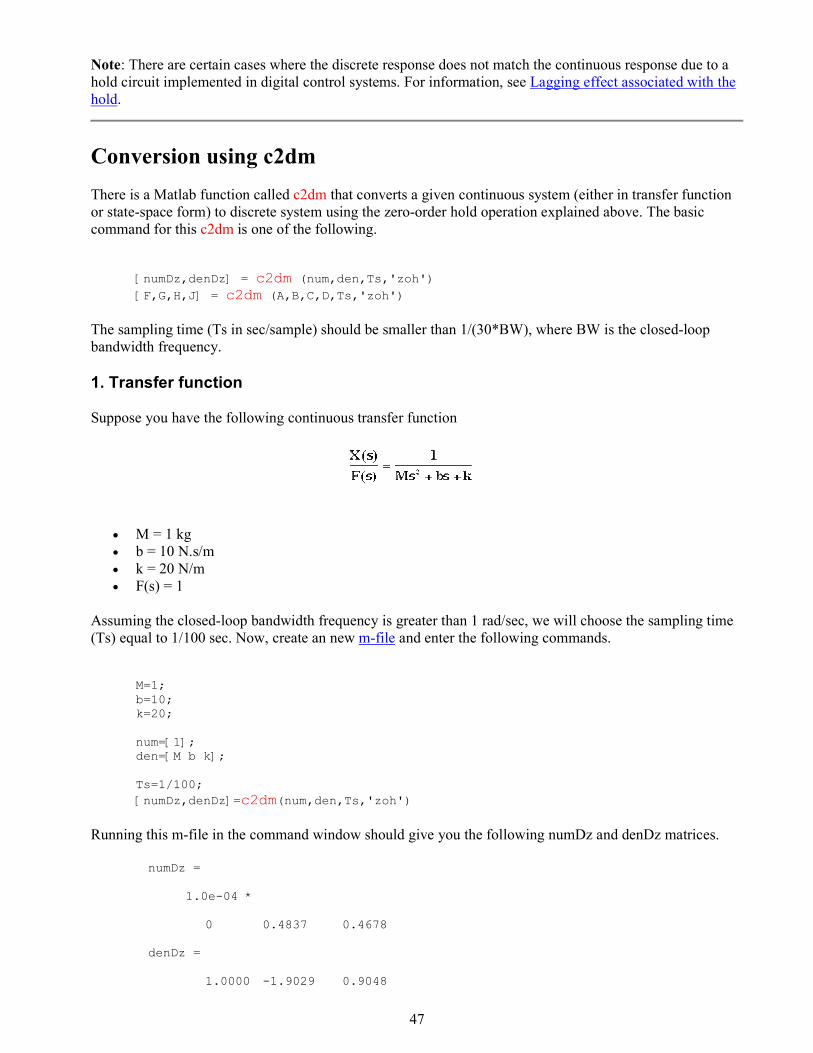
1. Transfer function

Suppose you have the following continuous transfer function

• M = 1 kg

• b = 10 N.s/m

• k = 20 N/m

• F(s) = 1

Assuming the closed-loop bandwidth frequency is greater than 1 rad/sec, we will choose the sampling time

(Ts) equal to 1/100 sec. Now, create an new m-file and enter the following commands.

M=1;

b=10;

k=20;

num=[1];

den=[M b k];

Ts=1/100;

[numDz,denDz]=c2dm(num,den,Ts,'zoh')

Running this m-file in the command window should give you the following numDz and denDz matrices.

numDz =

1.0e-04 *

0 0.4837 0.4678

denDz =

1.0000 -1.9029 0.9048

48

From these matrices, the discrete transfer function can be written as

Note: The numerator and denominator matrices will be represented by the descending powers of z. For

more information on Matlab representation, please refer to Matlab representation.

Now you have the transfer function in discrete form.

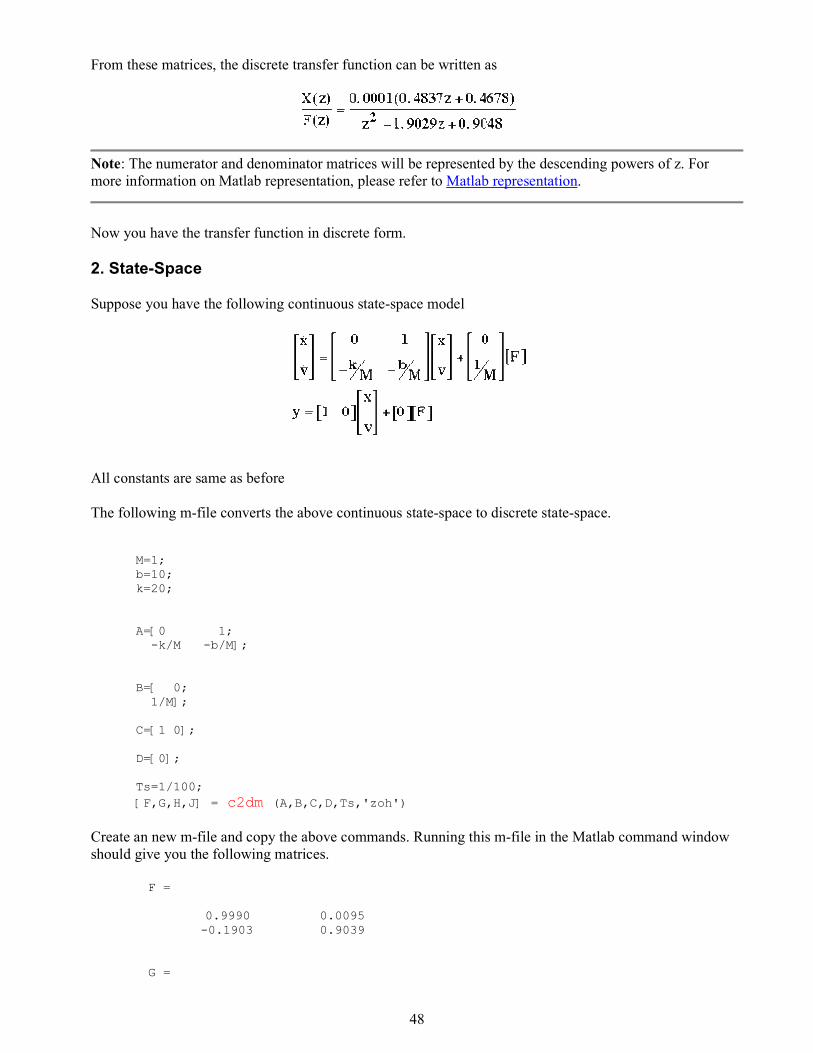
2. State-Space

Suppose you have the following continuous state-space model

All constants are same as before

The following m-file converts the above continuous state-space to discrete state-space.

M=1;

b=10;

k=20;

A=[0 1;

-k/M -b/M];

B=[ 0;

1/M];

C=[1 0];

D=[0];

Ts=1/100;

[F,G,H,J] = c2dm (A,B,C,D,Ts,'zoh')

Create an new m-file and copy the above commands. Running this m-file in the Matlab command window

should give you the following matrices.

F =

0.9990 0.0095

-0.1903 0.9039

G =

49

0.0000

0.0095

H =

1 0

J =

0

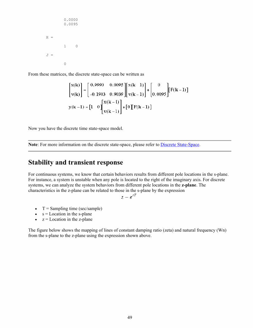
From these matrices, the discrete state-space can be written as

Now you have the discrete time state-space model.

Note: For more information on the discrete state-space, please refer to Discrete State-Space.

Stability and transient response

For continuous systems, we know that certain behaviors results from different pole locations in the s-plane.

For instance, a system is unstable when any pole is located to the right of the imaginary axis. For discrete

systems, we can analyze the system behaviors from different pole locations in the z-plane. The

characteristics in the z-plane can be related to those in the s-plane by the expression

• T = Sampling time (sec/sample)

• s = Location in the s-plane

• z = Location in the z-plane

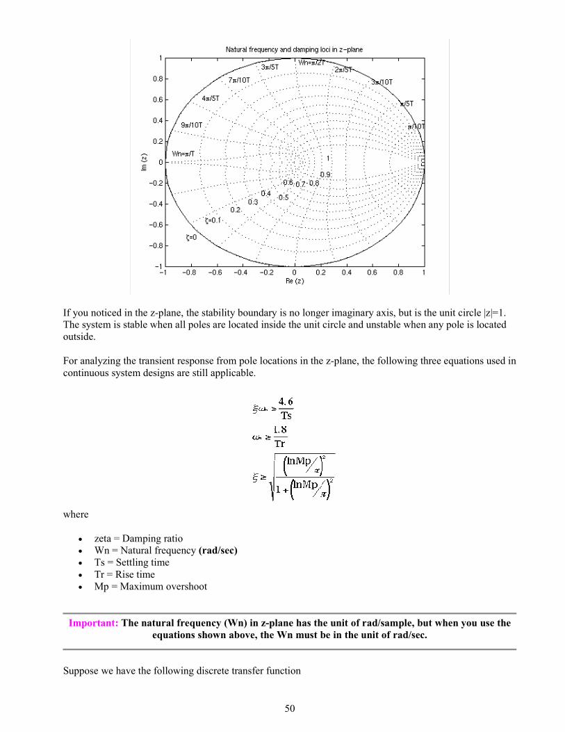
The figure below shows the mapping of lines of constant damping ratio (zeta) and natural frequency (Wn)

from the s-plane to the z-plane using the expression shown above.

50

If you noticed in the z-plane, the stability boundary is no longer imaginary axis, but is the unit circle |z|=1.

The system is stable when all poles are located inside the unit circle and unstable when any pole is located

outside.

For analyzing the transient response from pole locations in the z-plane, the following three equations used in

continuous system designs are still applicable.

where

• zeta = Damping ratio

• Wn = Natural frequency (rad/sec)

• Ts = Settling time

• Tr = Rise time

• Mp = Maximum overshoot

Important: The natural frequency (Wn) in z-plane has the unit of rad/sample, but when you use the

equations shown above, the Wn must be in the unit of rad/sec.

Suppose we have the following discrete transfer function

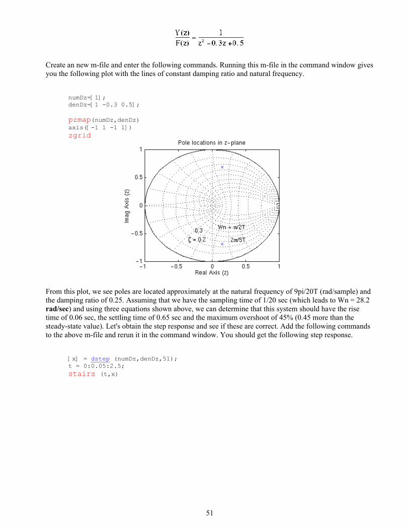
51

Create an new m-file and enter the following commands. Running this m-file in the command window gives

you the following plot with the lines of constant damping ratio and natural frequency.

numDz=[1];

denDz=[1 -0.3 0.5];

pzmap(numDz,denDz) axis([-1 1 -1 1])

zgrid

From this plot, we see poles are located approximately at the natural frequency of 9pi/20T (rad/sample) and

the damping ratio of 0.25. Assuming that we have the sampling time of 1/20 sec (which leads to Wn = 28.2

rad/sec) and using three equations shown above, we can determine that this system should have the rise

time of 0.06 sec, the settling time of 0.65 sec and the maximum overshoot of 45% (0.45 more than the

steady-state value). Let's obtain the step response and see if these are correct. Add the following commands

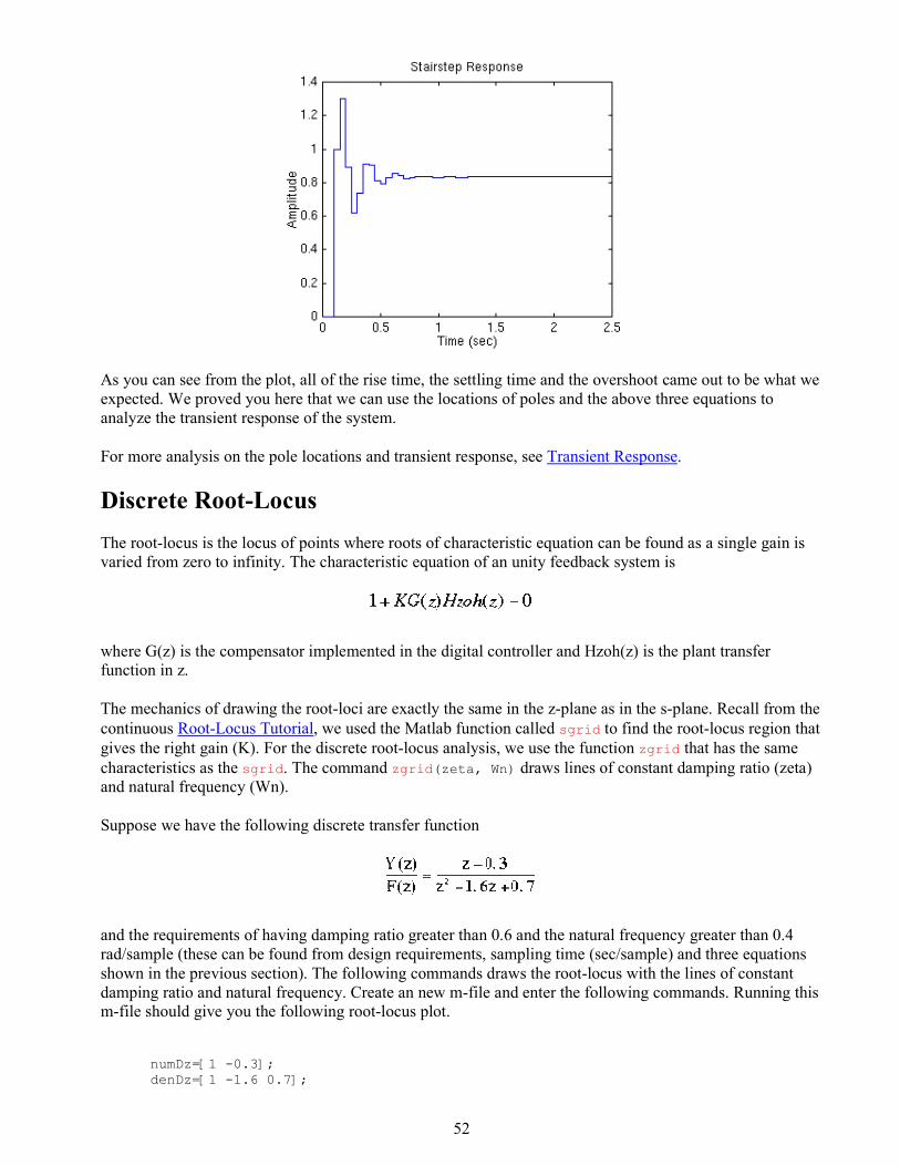
to the above m-file and rerun it in the command window. You should get the following step response.

[x] = dstep (numDz,denDz,51);

t = 0:0.05:2.5;

stairs (t,x)

52

As you can see from the plot, all of the rise time, the settling time and the overshoot came out to be what we

expected. We proved you here that we can use the locations of poles and the above three equations to

analyze the transient response of the system.

For more analysis on the pole locations and transient response, see Transient Response.

Discrete Root-Locus

The root-locus is the locus of points where roots of characteristic equation can be found as a single gain is

varied from zero to infinity. The characteristic equation of an unity feedback system is

where G(z) is the compensator implemented in the digital controller and Hzoh(z) is the plant transfer

function in z.

The mechanics of drawing the root-loci are exactly the same in the z-plane as in the s-plane. Recall from the

continuous Root-Locus Tutorial, we used the Matlab function called sgrid to find the root-locus region that

gives the right gain (K). For the discrete root-locus analysis, we use the function zgrid that has the same

characteristics as the sgrid. The command zgrid(zeta, Wn) draws lines of constant damping ratio (zeta)

and natural frequency (Wn).

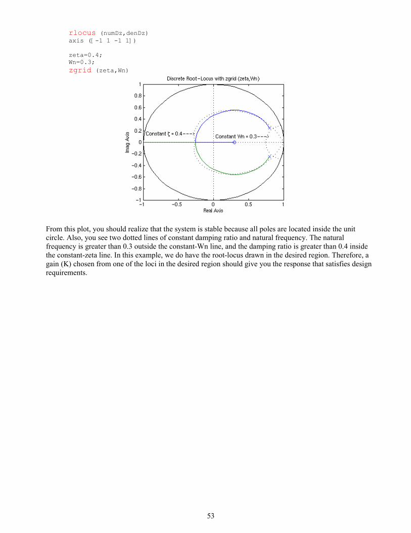
Suppose we have the following discrete transfer function

and the requirements of having damping ratio greater than 0.6 and the natural frequency greater than 0.4

rad/sample (these can be found from design requirements, sampling time (sec/sample) and three equations

shown in the previous section). The following commands draws the root-locus with the lines of constant

damping ratio and natural frequency. Create an new m-file and enter the following commands. Running this

m-file should give you the following root-locus plot.

numDz=[1 -0.3];

denDz=[1 -1.6 0.7];

53

rlocus (numDz,denDz) axis ([-1 1 -1 1])

zeta=0.4;

Wn=0.3;

zgrid (zeta,Wn)

From this plot, you should realize that the system is stable because all poles are located inside the unit

circle. Also, you see two dotted lines of constant damping ratio and natural frequency. The natural

frequency is greater than 0.3 outside the constant-Wn line, and the damping ratio is greater than 0.4 inside

the constant-zeta line. In this example, we do have the root-locus drawn in the desired region. Therefore, a

gain (K) chosen from one of the loci in the desired region should give you the response that satisfies design

requirements.