
Maths for Intelligent Systems - ipvs.informatik.uni ... · Maths for Intelligence Systems, Marc...
109
Maths for Intelligent Systems Marc Toussaint January, 2017 Contents 1 Speaking Maths 4 1.1 Describing systems ................................. 4 1.2 Should maths be tought with many application examples? Or abstractly? .. 5 1.3 Notation: Some seeming trivialities ........................ 5 2 Linear Algebra 6 2.1 Vector Spaces ..................................... 6 Why should we care for vector spaces in intelligent systems research? (6) What is a vector? (7) What is a vector space? (7) 2.2 Vectors, dual vectors, coordinates, matrices, tensors ............... 8 A taxonomy of linear functions (8) Bases and coordinates (9) The dual vector space – and its coordinates (10) Coordinates for every linear thing: tensors (10) Finally: Matrices (11) Coordinate transformations (12) 2.3 Scalar product and orthonormal basis ....................... 13 Properties of orthonormal bases (14) 2.4 The Structure of Transforms & Singular Value Decomposition ......... 16 The Singular Value Decomposition Theorem (16) 2.5 Point of departure from the coordinate-free notation .............. 18 2.6 Filling SVD with life ................................. 18 Understand vv > as projection (18) SVD for symmetric matrices (19) SVD for general matrices (20) 2.7 Eigendecomposition ................................. 21 Power Method (22) Power Method including the smallest eigenvalue (22) Why should I care about Eigenvalues and Eigenvectors? (22)
Transcript of Maths for Intelligent Systems - ipvs.informatik.uni ... · Maths for Intelligence Systems, Marc...
Maths for Intelligent Systems
Marc Toussaint
January, 2017
Contents
1 Speaking Maths 4
1.1 Describing systems . . . . . . . . . . . . . . . . . . . . . . . . . . . . . . . . . 4
1.2 Should maths be tought with many application examples? Or abstractly? . . 5
1.3 Notation: Some seeming trivialities . . . . . . . . . . . . . . . . . . . . . . . . 5
2 Linear Algebra 6
2.1 Vector Spaces . . . . . . . . . . . . . . . . . . . . . . . . . . . . . . . . . . . . . 6
Why should we care for vector spaces in intelligent systems research? (6) Whatis a vector? (7) What is a vector space? (7)
2.2 Vectors, dual vectors, coordinates, matrices, tensors . . . . . . . . . . . . . . . 8
A taxonomy of linear functions (8) Bases and coordinates (9) The dual vectorspace – and its coordinates (10) Coordinates for every linear thing: tensors (10)Finally: Matrices (11) Coordinate transformations (12)
2.3 Scalar product and orthonormal basis . . . . . . . . . . . . . . . . . . . . . . . 13
Properties of orthonormal bases (14)
2.4 The Structure of Transforms & Singular Value Decomposition . . . . . . . . . 16
The Singular Value Decomposition Theorem (16)
2.5 Point of departure from the coordinate-free notation . . . . . . . . . . . . . . 18
2.6 Filling SVD with life . . . . . . . . . . . . . . . . . . . . . . . . . . . . . . . . . 18
Understand vv> as projection (18) SVD for symmetric matrices (19) SVD forgeneral matrices (20)
2.7 Eigendecomposition . . . . . . . . . . . . . . . . . . . . . . . . . . . . . . . . . 21
Power Method (22) Power Method including the smallest eigenvalue (22) Whyshould I care about Eigenvalues and Eigenvectors? (22)
1

2 Maths for Intelligence Systems, Marc Toussaint
2.8 Point of Departure: Numerics to compute these things . . . . . . . . . . . . . 23
2.9 Examples and Exercises . . . . . . . . . . . . . . . . . . . . . . . . . . . . . . . 23
Matrix equations (23) Examples for Vector Spaces (voluntary, discussed on Oct23rd) (24) Basis (24) From the Robotics Course (voluntary) (24) Bases for Poly-nomials (25) Projections (26) SVD (26) Covariance and PCA (27) Bonus: Scalarproduct and Orthogonality (27) Eigenvectors (27) RKHS (28)
3 Derivatives 29
3.1 The coordinate-free view: The meaning of life for a derivative is to eat a vectorand output a scalar . . . . . . . . . . . . . . . . . . . . . . . . . . . . . . . . . 29
3.2 Don’t confuse partial and total derivative . . . . . . . . . . . . . . . . . . . . . 29
Partial derivative (29) Chain Rule, computation graphs and the total derivative (30)
3.3 Gradient, Jacobian, Hessian, Taylor Expansion . . . . . . . . . . . . . . . . . . 32
Gradient, Jacobian, and Hessian (32) Taylor expansion (33)
3.4 Contra- and co-variance . . . . . . . . . . . . . . . . . . . . . . . . . . . . . . . 34
3.5 Steepest descent and the covariant gradient vector . . . . . . . . . . . . . . . 36
3.6 Derivative Rules and Examples . . . . . . . . . . . . . . . . . . . . . . . . . . 37
GP regression (38) Logistic regression (38)
3.7 Check your gradients numerically! . . . . . . . . . . . . . . . . . . . . . . . . 39
3.8 Examples and Exercises . . . . . . . . . . . . . . . . . . . . . . . . . . . . . . . 40
More derivatives (40) Minima (40) Multivariate Calculus (40) Finite Differ-ence Gradient Checking (41) Backprop in a Neural Net (41) Backprop in a Neu-ral Net (41) Logistic Regression Gradient & Hessian (42)
4 Optimization 43
4.1 Downhill algorithms for unconstrained optimization . . . . . . . . . . . . . . 43
Why you shouldn’t trust the magnitude of the gradient (43) Ensuring monotoneand sufficient decrease: Backtracking line search, Wolfe conditions, & convergence(44) The Newton direction (45) Gauss-Newton: a super important special case(48) Quasi-Newton & BFGS: approximating the hessian from gradient observa-tions (49) Conjugate Gradient (50) Rprop* (51)
4.2 The general optimization problem – a mathematical program . . . . . . . . . 52
4.3 The KKT conditions . . . . . . . . . . . . . . . . . . . . . . . . . . . . . . . . . 53
4.4 Unconstrained problems to tackle a constrained problem . . . . . . . . . . . . 54
Augmented Lagrangian* (55)
4.5 The Lagrangian . . . . . . . . . . . . . . . . . . . . . . . . . . . . . . . . . . . 56
How the Lagrangian relates to the KKT conditions (56) Solving mathematicalprograms analytically, on paper. (57) Solving the dual problem, instead of theprimal. (58) Finding the “saddle point” directly with a primal-dual Newton
Maths for Intelligence Systems, Marc Toussaint 3
method. (58) Log Barriers and the Lagrangian (59)
4.6 Convex Problems . . . . . . . . . . . . . . . . . . . . . . . . . . . . . . . . . . 60
Convex sets, functions, problems (61) Linear and quadratic programs (61) TheSimplex Algorithm (63) Sequential Quadratic Programming (64)
4.7 Blackbox & Global Optimization: It’s all about learning . . . . . . . . . . . . . 65
A sequential decision problem formulation (65) Acquisition Functions for BayesianGlobal Optimization* (66) Classical model-based blackbox optimization (non-global)* (68) Evolutionary Algorithms* (69)
4.8 Examples and Exercises . . . . . . . . . . . . . . . . . . . . . . . . . . . . . . . 69
Convergence proof (69) Backtracking Line Search (70) Gauss-Newton (71) Robustunconstrained optimization (71) Lagrangian Method of Multipliers (72) Lagrangianand dual function (72) Equality Constraint Penalties and Augmented Lagrangian(73) Optimize a constrained problem (73) Network flow problem (74) Minimumfuel optimal control (74) Voluntary: Reformulating Norms (75) Voluntary: Somemore examples (75) Restarts of Local Optima (75) UCB Bayesian Optimization(76) No Free Lunch Theorems (76)
5 Probabilities & Information 76
5.1 Basics . . . . . . . . . . . . . . . . . . . . . . . . . . . . . . . . . . . . . . . . . 76
Axioms, definitions, Bayes rule (77) Standard discrete distributions (78) Conjugatedistributions (79) Distributions over continuous domain (79) Gaussian (80) “Particledistribution” (81)
5.2 Between probabilities and optimization: neg-log-probabilities, exp-neg-energies,exponential family, Gibbs and Boltzmann . . . . . . . . . . . . . . . . . . . . . 83
5.3 Information, Entropie & Kullback-Leibler . . . . . . . . . . . . . . . . . . . . . 86
5.4 The Laplace approximation: A 2nd-order Taylor of log p . . . . . . . . . . . . 87
5.5 Variational Inference . . . . . . . . . . . . . . . . . . . . . . . . . . . . . . . . 88
5.6 The Fisher information metric: 2nd-order Taylor of the KLD . . . . . . . . . . 88
5.7 Examples and Exercises . . . . . . . . . . . . . . . . . . . . . . . . . . . . . . . 88
Maximum Entropy and Maximum Likelihood (89) Maximum likelihood and KL-divergence (90) Laplace Approximation (90) Learning = Compression (91) Agzip experiment (91) Maximum Entropy and ML (91)
A Gaussian identities 92
B 3D geometry basics (for robotics) 97
B.1 Rotations . . . . . . . . . . . . . . . . . . . . . . . . . . . . . . . . . . . . . . . 97
B.2 Transformations . . . . . . . . . . . . . . . . . . . . . . . . . . . . . . . . . . . 100
Static transformations (100) Dynamic transformations (101) A note on affinecoordinate frames (102)

4 Maths for Intelligence Systems, Marc Toussaint
B.3 Kinematic chains . . . . . . . . . . . . . . . . . . . . . . . . . . . . . . . . . . . 104
Rigid and actuated transforms (104) Jacobian & Hessian (105)
Index 108
1 Speaking Maths
1.1 Describing systems
Systems can be described in many ways. Biologists describe their systems oftenusing text, and lots and lots of data. Architects describe buildings using drawings.Physisics describe nature using differential equations, or optimality principles, ordifferential geometry and group theory. The whole point of science is to find de-scriptions of systems—in the natural science descriptions that allow prediction, inthe synthetic/engineering sciences descriptions that enable the design of good sys-tems, problem-solving systems.
And how should we describe intelligent systems? Robots, perception systems, ma-chine learning systems? I guess there are two main categories: the imperative wayin terms of literal algorithms (code), or the declarative way in terms of formulatingthe problem. I prefer the latter.
The point of this lecture is to teach you to speak maths, to use maths to describe sys-tems or problems. I feel that most maths courses rather teach to consume maths, orsolve mathematical problems, or prove things. Clearly, this is also important. Butfor the purpose of intelligent systems research, it is essential to be skilled in express-ing problems mathematically, before even thinking about resulting algorithms.
If you happen to attend a Machine Learning or Robotics course you’ll see that everyproblem is addressed the same way: You have an “intuitively formulated” prob-lem; the first step is to find a mathematical formulation; the second step to solve it.The second step is often technical. The first step is really the interesting and creativepart. This is where you have to nail down the problem, i.e., nail down what it meansto be intelligent/good/well-performing, and thereby describe “intelligence”—or atleast a tiny aspect of it.
The “Maths for Intelligent Systems” course will recap essentials of linear algebra,optimization, probabilities, and statistics. These fields are essential to formulateproblems in intelligent systems research and hopefully will equip you with thebasics of speaking maths.

Maths for Intelligence Systems, Marc Toussaint 5
1.2 Should maths be tought with many application examples? Orabstractly?
Maybe this is the wrong question and implies a view on maths I don’t agree with.I think (but this is agruable) maths is nothing but abstractions of real-world things.At least I aim to teach maths as abstractions of real-world things. It is misleadingto think that there is “pure maths” and then “applications”. Instead mathematicalconcepts, such as a vector, are abstractions of real-world things, such as cars, faces,scenes, images, documents; and theorems, methods and algorithms that apply onvectors of course also apply to all the real-world things—subject to the limitationsof this abstraction. So, the goal is not to teach you a lookup table of which methodcan be used in which application, but rather to teach which concepts maths offers toabstract real-world things—so that you find such abstractions yourself once you’llhave to solve a real-world problem.
1.3 Notation: Some seeming trivialities
Equations and mathematical expressions have a syntax. This is hardly ever madeexplicit1 and might seem trivial. But it is surprising how buggy mathematical state-ments can be in scientific papers (and oral exams). I don’t want to write much textabout this, just some bullet points:
• Always declare objects.
• Be aware of variable/index scoping. For instance, if you have an equation,and one side includes a variable i, the other doesn’t, this often is a notationalbug. (Unless this equation incidently makes a statement about independenceon i.)
• Type checking. Within an equation, be sure to know exactly of what type eachterm is: vector? matrix? scalar? tensor?
• Decorations are ok, but really not necessary. It is much more important todeclare all things. E.g., there are all kinds of decorations used for vectors,v, v,−→v , |v〉 and matrices. But these are not necessary. Properly declaring allsymbols is much more important.
• sets: xini=1, tuples: (xi)ni=1, (x1, .., xn), x1:n
• set notations f(x) : x ∈ R, n ∈ N : ∃ vini=1 linearly independent, vi ∈ V
• indicator functions [a = b] or I(a = b) and Kronecker δab
• (a, b) ∈ A×B,
1Except perhaps by Godel’s incompleteness theorems and areas like automated theorem proving.

6 Maths for Intelligence Systems, Marc Toussaint
• outer product x ⊗ y ∈ X × Y is almost the same as (x, y) ∈ X × Y (slightlydifferent in standard vector and tensor context); don’t confuse with the crossproduct in 3D!
• direct sum A⊕B is same as A×B in finite-dimensional spaces
• write argmin instead of argmin
• Never use multiple letters for one thing. E.g. length = 3 means l times e timesn times g times t times h equals 3.
• Difference between→ and 7→
f : R→ R, x 7→ cos(x)
• The dot thing:
f : A×B → C , f(a, ·) : B → C, b 7→ f(a, b)
The dot is in particular used for the inner product (a 2-form): 〈·, ·〉 : V ×V → R
• The p-norm ||x||p = [∑i x
pi ]
1/p. By default p = 2, that is ||x|| = ||x||2 = |x|,which is the length of a vector. When saying “2-norm”, I often actually mean||x||2 =
∑i x
2i .
• diag(a1, .., an) =
a1 0
. . .0 an
• A typical convention is
0n = (0, .., 0) ∈ Rn , 1n = (1, .., 1) ∈ Rn , In = diag(1n)
Also, ei = (0, .., 0, 1, 0, .., 0) ∈ Rn often denotes the ith column of the identitymatrix, which of course are the coordinates of a basis vector ei ∈ V in a basis(ei)
ni=1.
• The element-wise product of two matricies A and B is also called Hadamardproduct and notatedAB (which has nothing to do with the concatenation oftwo operations!). If there is need, perhaps also use this to notate the element-wise product of two vectors.
2 Linear Algebra
2.1 Vector Spaces
2.1.1 Why should we care for vector spaces in intelligent systems research?
We want to describe intelligent systems. For this we describe systems, or aspects ofsystems, as elements of a space:
Maths for Intelligence Systems, Marc Toussaint 7
– The input space X , output space Y in ML
– The space of functions (or classifiers) f : X → Y in ML
– The space of world states S and actions A in Reinforcement Learning
– The space of policies π : S → A in RL
– The space of feedback controllers π : x 7→ u in robot control
– The configuration space Q of a robot
– The space of paths x : [0, 1]→ Q in robotics
– The space of image segmentations s : I → 0, 1 in computer vision
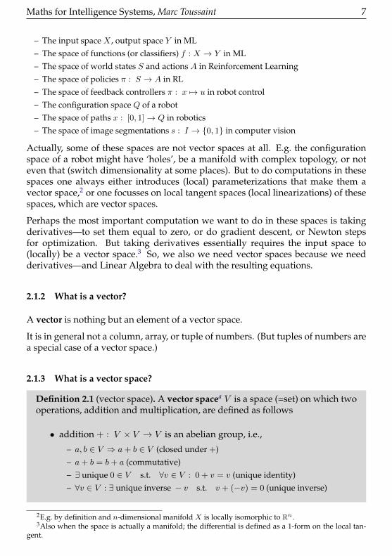
Actually, some of these spaces are not vector spaces at all. E.g. the configurationspace of a robot might have ‘holes’, be a manifold with complex topology, or noteven that (switch dimensionality at some places). But to do computations in thesespaces one always either introduces (local) parameterizations that make them avector space,2 or one focusses on local tangent spaces (local linearizations) of thesespaces, which are vector spaces.
Perhaps the most important computation we want to do in these spaces is takingderivatives—to set them equal to zero, or do gradient descent, or Newton stepsfor optimization. But taking derivatives essentially requires the input space to(locally) be a vector space.3 So, we also we need vector spaces because we needderivatives—and Linear Algebra to deal with the resulting equations.
2.1.2 What is a vector?
A vector is nothing but an element of a vector space.
It is in general not a column, array, or tuple of numbers. (But tuples of numbers area special case of a vector space.)
2.1.3 What is a vector space?
Definition 2.1 (vector space). A vector spacea V is a space (=set) on which twooperations, addition and multiplication, are defined as follows
• addition + : V × V → V is an abelian group, i.e.,
– a, b ∈ V ⇒ a+ b ∈ V (closed under +)
– a+ b = b+ a (commutative)
– ∃ unique 0 ∈ V s.t. ∀v ∈ V : 0 + v = v (unique identity)
– ∀v ∈ V : ∃ unique inverse − v s.t. v + (−v) = 0 (unique inverse)
2E.g. by definition and n-dimensional manifold X is locally isomorphic to Rn.3Also when the space is actually a manifold; the differential is defined as a 1-form on the local tan-
gent.

8 Maths for Intelligence Systems, Marc Toussaint
• multiplication · : R× V → V fulfils, for α, β ∈ R,α(βv) = (αβ)v , 1v = v , α(v + w) = αv + αw
aWe only consider vector spaces over R.
Roughly, this definition says that a vector space is “closed under linear transforma-tions”, meaning that we can add and scale vectors and they remain vectors.
2.2 Vectors, dual vectors, coordinates, matrices, tensors
In this section we explain what might be obvious: that once we have a basis, wecan write vectors as (column) coordinate vectors, 1-forms as (row) coordinate vec-tors, and linear transformations as matrices. Only the last subsection becomes morepractical, refers to concrete exercises, and explains how in practise not to get con-fused about basis transforms and coordinate representations in different bases. Soa practically oriented reader might want to skip to the last subsection.
2.2.1 A taxonomy of linear functions
For simplicity we consider only functions involving a single vector space V . But allthat is said transfers to the case when multiple vector spaces V,W, ...were involved.
Definition 2.2. f : V → X linear ⇐⇒ f(αv + βw) = αf(v) + βf(w), whereX is any other vector space (e.g. X = R, or X = V × V ).
Definition 2.3. f : V × V × · · · × V → X multi-linear ⇐⇒ f is linear in eachinput.
Many names are used for special linear functions—let’s make some explicit:
– f : V → R, called linear functional4, or 1-form, or dual vector.
– f : V → V , called linear map, or linear transform, or vector-valued 1-form
– f : V × V → R, called bilinear functional, or 2-form
– f : V × V × V → R, called 3-form (or unspecifically ’multi-linear functional’)
– f : V × V → V , called vector-valued 2-form (or unspecifically ’multi-linear map’)
– f : V × V × V → V × V , called bivector-valued 3-form
– f : V k → V m, called m-vector-valued k-form
This gives us a simple taxonomy of linear functions based on how many vectors afunction eats, and how many it outputs. To give examples, consider some space Xof systems (examples above), which might itself not be a vector space. But locally,around a specific x ∈ X , its tangent V is a vector space. Then
4The word ’functional’ instead of ’function’ is especially used when V is a space of functions.

Maths for Intelligence Systems, Marc Toussaint 9
– f : X → R could be a cost function over the system space.
– The differential df |x : V → R is a 1-form, telling us how f changes when ‘making atangent step’ v ∈ V .
– The 2nd derivative d2f |x : V × V → R is a 2-form, telling us how df |x(v) changes when‘making a tangent step’ w ∈ V .
– The inner product 〈·, ·〉 : V × V → R is a 2-form.
This is simply to show that 1- and 2-forms are very common things. Another ex-ample:
– f : Ri → Ro is a neural network that maps i input signals to o output signals.
– Its derivative df |x : Ri → Ro is a vector-valued 1-form, telling us how each outputchanges with a step v ∈ Ri in the input.
– Its 2nd derivative d2f |x : Ri × Ri → Ro is a vector-valued 2-form.
This is simply to show that vector-valued functions, 1-forms, and 2-forms are com-mon. Instead of being a neural network, f could also be a mapping from one pa-rameterization of a system to another, or the mapping from the joint angles of arobot to its hand position.
2.2.2 Bases and coordinates
We need to define some notions. I’m not commenting these definitions—train your-self in reading maths...
Definition 2.4. span(viki=1) = ∑i αivi : αi ∈ R
Definition 2.5. vini=1 linearly independent ⇐⇒[∑
i αivi = 0⇒ ∀iαi = 0]
Definition 2.6. dim(V ) = maxnn ∈ N : ∃ vini=1 lin.indep., vi ∈ V
Definition 2.7. B = (ei)ni=1 is a basis of V ⇐⇒ span(B) = V andB lin.indep.
Definition 2.8. The tuple (v1, v2, .., vn) ∈ Rn is called coordinates of v ∈ V inthe basis (ei)
ni=1 iff v =
∑i viei
Given a basis (ei)ni=1, we can describe every vector v as a linear combination v =∑
i viei of basic elements—the basis vectors ei. This general idea, that “linear things”can be described as linear combinations of “basic elements” carries over also tofunctions. In fact, to all the types of functions we described above: 1-forms, 2-forms,bi-vector-valued k-forms, whatever. And if we describe all these als linear com-binations of basic elements we automatically also introduce coordinates for thesethings. To get there, we first have to introduce a second type of “basic elements”:dual vectors.
10 Maths for Intelligence Systems, Marc Toussaint
2.2.3 The dual vector space – and its coordinates
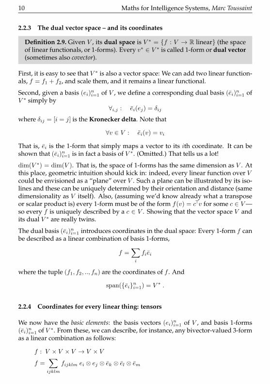
Definition 2.9. Given V , its dual space is V ∗ = f : V → R linear (the spaceof linear functionals, or 1-forms). Every v∗ ∈ V ∗ is called 1-form or dual vector(sometimes also covector).
First, it is easy to see that V ∗ is also a vector space: We can add two linear function-als, f = f1 + f2, and scale them, and it remains a linear functional.
Second, given a basis (ei)ni=1 of V , we define a corresponding dual basis (ei)
ni=1 of
V ∗ simply by∀i,j : ei(ej) = δij
where δij = [i = j] is the Kronecker delta. Note that
∀v ∈ V : ei(v) = vi
That is, ei is the 1-form that simply maps a vector to its ith coordinate. It can beshown that (ei)
ni=1 is in fact a basis of V ∗. (Omitted.) That tells us a lot!
dim(V ∗) = dim(V ). That is, the space of 1-forms has the same dimension as V . Atthis place, geometric intuition should kick in: indeed, every linear function over Vcould be envisioned as a “plane” over V . Such a plane can be illustrated by its iso-lines and these can be uniquely determined by their orientation and distance (samedimensionality as V itself). Also, (assuming we’d know already what a transposeor scalar product is) every 1-form must be of the form f(v) = c>v for some c ∈ V—so every f is uniquely described by a c ∈ V . Showing that the vector space V andits dual V ∗ are really twins.
The dual basis (ei)ni=1 introduces coordinates in the dual space: Every 1-form f can
be described as a linear combination of basis 1-forms,
f =∑i
fiei
where the tuple (f1, f2, .., fn) are the coordinates of f . And
span(eini=1) = V ∗ .
2.2.4 Coordinates for every linear thing: tensors
We now have the basic elements: the basis vectors (ei)ni=1 of V , and basis 1-forms
(ei)ni=1 of V ∗. From these, we can describe, for instance, any bivector-valued 3-form
as a linear combination as follows:
f : V × V × V → V × V
f =∑ijklm
fijklm ei ⊗ ej ⊗ ek ⊗ el ⊗ em
Maths for Intelligence Systems, Marc Toussaint 11
The ⊗ is called outer product (or tensor product), and v ⊗ w ∈ V ×W if V and Ware finite vector spaces. For our purposes, we may think of v ⊗ w = (v, w) simplyas the tuple of both. Therefore ei ⊗ ej ⊗ ek ⊗ el ⊗ em is a 5-tuple and we have intotal n5 such basis objects—and fijklm denotes the corresponding n5 coordinates.The first two indices are contra-variant, the last three covariant—these notions areexplained in detail later.
2.2.5 Finally: Matrices
As a special case of the above, every f : V → U can be described as a linear combi-nation
f =∑ij
fij ei ⊗ ej ,
where (ej)nj=1 is a basis of V ∗ and (ei) a basis of U .
Let’s see how this fits with some easier view, without all this fuss about 1-forms.We already understood that the operator ej(v) = vj simply picks the jth coordinateof a vector. Therefore
f(v) =[∑ij
fij ei ⊗ ej](v) =
∑ij
fij eivj .
In case it helps, we can ‘derive’ this more slowly as
f(v) = f(∑k
vkek) =∑k
vkf(ek) =∑k
vk
[∑ij
fij ei ⊗ ej]ek (1)
=∑ijk
fij vk ei ej(ek) =∑ijk
fij vk ei δjk =∑i
[∑j
fij vj
]ei . (2)
As a result, this tells us that the vector u = f(v) ∈ V has the coordinates ui =∑j fij vj . And the vector f(ej) ∈ V has the coordinates fij , that is, f(ej) =
∑i fijei.
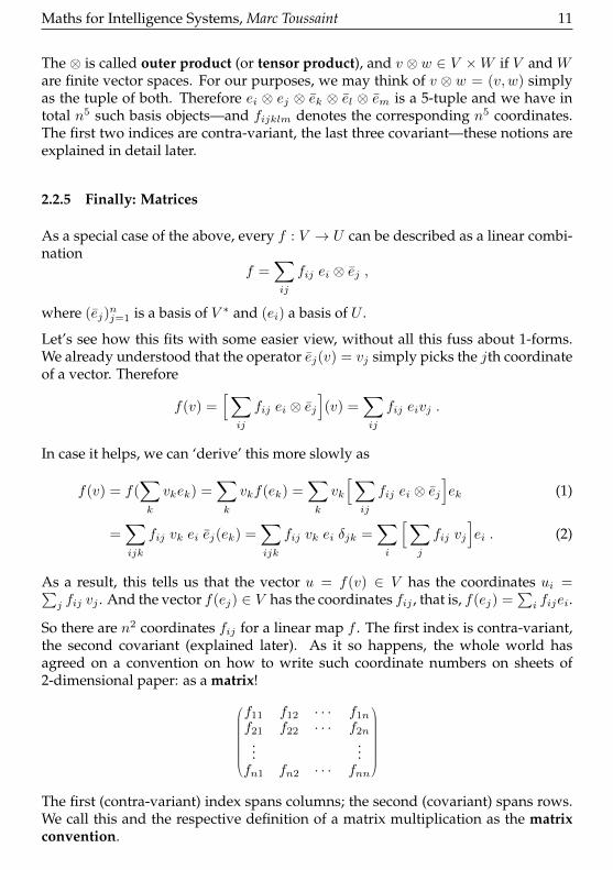
So there are n2 coordinates fij for a linear map f . The first index is contra-variant,the second covariant (explained later). As it so happens, the whole world hasagreed on a convention on how to write such coordinate numbers on sheets of2-dimensional paper: as a matrix!
f11 f12 · · · f1n
f21 f22 · · · f2n
......
fn1 fn2 · · · fnn
The first (contra-variant) index spans columns; the second (covariant) spans rows.We call this and the respective definition of a matrix multiplication as the matrixconvention.
12 Maths for Intelligence Systems, Marc Toussaint
Note that the identity map I : V → V can be written as
I =∑i
ei ⊗ ei , Iij = δij . (3)
Equally, the (contra-variant) coordinates of a vector are written as columns
v1
v2
...vn
and the (covariant) coordinates of a 1-form h : V → R as a row
(h1 h2 · · · hn)
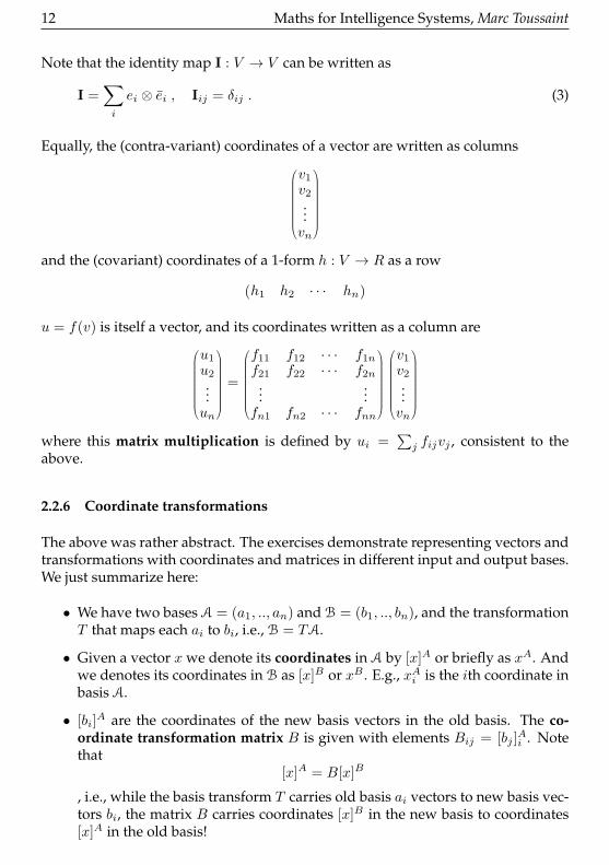
u = f(v) is itself a vector, and its coordinates written as a column are
u1
u2
...un
=
f11 f12 · · · f1n
f21 f22 · · · f2n
......
fn1 fn2 · · · fnn
v1
v2
...vn
where this matrix multiplication is defined by ui =∑j fijvj , consistent to the
above.
2.2.6 Coordinate transformations
The above was rather abstract. The exercises demonstrate representing vectors andtransformations with coordinates and matrices in different input and output bases.We just summarize here:
• We have two bases A = (a1, .., an) and B = (b1, .., bn), and the transformationT that maps each ai to bi, i.e., B = TA.
• Given a vector x we denote its coordinates in A by [x]A or briefly as xA. Andwe denotes its coordinates in B as [x]B or xB . E.g., xAi is the ith coordinate inbasis A.
• [bi]A are the coordinates of the new basis vectors in the old basis. The co-
ordinate transformation matrix B is given with elements Bij = [bj ]Ai . Note
that[x]A = B[x]B
, i.e., while the basis transform T carries old basis ai vectors to new basis vec-tors bi, the matrix B carries coordinates [x]B in the new basis to coordinates[x]A in the old basis!

Maths for Intelligence Systems, Marc Toussaint 13
• Given a linear transformation f in the vector space, we can represent it asa matrix in four ways, using basis A or B in the input and output spaces,respectively. If [f ]AA = F is the matrix in old coordinates (using A for inputand output), then [f ]BB = B-1FB is its matrix in new coordinates, [f ]AB =FB is its matrix using B for the input and A for the output space, and [f ]BA =B-1F is the matrix using A for input and B for output space.
• T itself is also a linear transform. [T ]AA = B is its matrix in old coordinates.And the same [T ]BB = B is also its matrix in new coordinates! [T ]BA = I isits matrix when using A for input and B for output space. And [T ]AB = B2
is its matrix using B for input and A for output space.
rows columnseat a vector generate a vector
1-formvectorco-vector
derivativeinput space output space
contra-variant co-variantco-variant coordinates contra-variant coordinates
2.3 Scalar product and orthonormal basis
Please note that so far we have not in any way referred to a scalar product or atranspose. All the concepts above, dual vector space, bases, coordinates, matrix-vector multiplication, are fully independent of the notion of a scalar product ortranspose. Columns and rows naturally appear as coordinates of vectors and 1-forms. But now we need to introduce scalar products.
Definition 2.10. A scalar product (also called inner product) of V is a symmet-ric positive definite 2-form
〈·, ·〉 : V × V → R .
with 〈v, w〉 = 〈w, v〉 and 〈v, v〉 > 0 for all v 6= 0 ∈ V .
Definition 2.11. Given a scalar product, we define for every v ∈ V its dualv∗ ∈ V ∗ as
v∗ = 〈v, ·〉 =∑i
vi〈ei, ·〉 =∑i
vie∗i .
Note that ei and e∗i are in general different 1-forms! The canonical dual basis (ei)ni=1
is independent of an introduction of a scalar product, they were the basis to intro-
14 Maths for Intelligence Systems, Marc Toussaint
duce coordinates for linear functions, including matrices. And while such coordi-nates do depend on a choice of basis (ei)
ni=1, they do not depend on a choice of
scalar product.
The vectors (e∗i )ni=1 also form a basis for V ∗, but a different one to the canonical
basis, and one that depends on the notion of a scalar product. You can see this: thecoordinates vi of v∗ in the basis (e∗i )
ni=1 are identical to the coordinates vi of v in the
basis (ei)ni=1, but different to the coordinates (v∗)i of v∗ in the basis (ei)
ni=1.
Definition 2.12. Given a scalar product, a set of vectors vini=1 is called or-thonormal iff 〈vi, vj〉 = δij .
Definition 2.13. Given a scalar product and basis (ei)ni=1, we define the metric
tensor gij = 〈ei, ej〉, which are the coordinates of the 2-form 〈·, ·〉, that is
〈·, ·〉 =∑ij
gij ei ⊗ ej .
This also implies that
〈v, w〉 =∑ij
viwj〈ei, ej〉 =∑ij
viwjgij = v>Gw .
Although related, do not confuse gij with the usual definition of a metric d(·, ·) in ametric space.
2.3.1 Properties of orthonormal bases
If we have an orthonormal basis (ei)ni=1, many thing simplify a lot. Throughout this
subsection, we assume ei orthonormal.
• The metric tensor gij = 〈ei, ej〉 = δij is the identity matrix.5 Such a metricis also called Euclidean. The norm ||εi|| = 1. The canonical dual basis (ei)
ni=1
and the one defined via the scalar product (e∗i )ni=1 become identical, ei = e∗i =
〈ei, ·〉. Consequently, v and v∗ have the same coordinates vi = (v∗)i w.r.t.(ei)
ni=1 respectively (ei)
ni=1.
• The coordinates of vectors can now easily been computed:
v =∑i
viei ⇒ 〈ei, v〉 = 〈ei,∑j
vjej〉 =∑j
〈ei, ej〉vj = vi (4)
5Being picky, a metric is not a matrix but a twice covariant tensor (a row of rows). That’s why it iscorrectly called metric tensor.
Maths for Intelligence Systems, Marc Toussaint 15
• The coordinates of a linear transform can equally easily been computed: Givena linear transform f : V → U an arbitrary (e.g. non-orthonormal) input basis(vi)
ni=1 of V , but an orthonormal basis (ui)
ni=1, then
f =∑ij
fijui ⊗ vj ⇒ (5)
〈ui, fvj〉 = 〈uj ,∑kl
fkluk ⊗ vl(vj)〉 =∑kl
fkl 〈uj , uk〉 vl(vj)
=∑kl
fklδjkδlj = fij (6)
• The projection onto a basis vector is given by ei〈ei, ·〉.
• The projection onto the span of several basis vectors (e1, .., ek) is given by∑ki=1 ei〈ei, ·〉.
• The identity mapping I : V → V is given by I =∑dim(V )i=1 ei〈ei, ·〉.
• The scalar product with an orthonormal basis is
〈v, w〉 =∑ij
viwjδij =∑i
viwi
which, using matrix convention, can also be written as
〈v, w〉 = (v1 v2 .. vn)
w1
w2
...wn
= v>w =
∑i
viwi ,
where for the first time we introduced the transpose which, in the matrixconvention, swaps columns to rows and rows to columns.
As a general note, a transposed vector “eats a vector and outputs a scalar”. Thatis v> : V → R should be thought of as a 1-form! Due to the matrix conventions,it generally is the case that “rows eat columns”, that is, every row index shouldalways be thought of as relating to a 1-form (dual vector), and every column indexas relating to a vector. That is totally consistent to our definition of coordinates.
For an orthonormal basis we also have
v∗(w) = 〈v, w〉 = v>w .
That is, v> is the coordinate representation of the 1-form v∗. (Which also says, thatthe coordinates of the 1-form v∗ in the special basis (e∗i )
ni=1 ⊂ V ∗ coincide with the
coordinates of the vector v.)
16 Maths for Intelligence Systems, Marc Toussaint
2.4 The Structure of Transforms & Singular Value Decomposition
We focus here on linear transforms (or “linear maps”) f : V → U from one vectorspace to another (or the same). It turns out that such transforms have a very specificand intuitive structure, which is captured by the singular value decompositon.
2.4.1 The Singular Value Decomposition Theorem
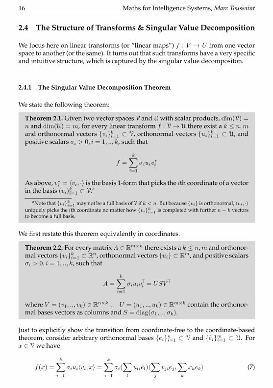
We state the following theorem:
Theorem 2.1. Given two vector spaces V and U with scalar products, dim(V) =n and dim(U) = m, for every linear transform f : V→ U there exist a k ≤ n,mand orthonormal vectors viki=1 ⊂ V, orthonormal vectors uiki=1 ⊂ U, andpositive scalars σi > 0, i = 1, .., k, such that
f =
k∑i=1
σiuiv∗i
As above, v∗i = 〈vi, ·〉 is the basis 1-form that picks the ith coordinate of a vectorin the basis (vi)
ki=1 ⊂ V.a
aNote that viki=1 may not be a full basis of V if k < n. But because vi is orthonormal, 〈vi, ·〉uniquely picks the ith coordinate no matter how viki=1 is completed with further n− k vectorsto become a full basis.
We first restate this theorem equivalently in coordinates.
Theorem 2.2. For every matrixA ∈ Rm×n there exists a k ≤ n,m and orthonor-mal vectors viki=1 ⊂ Rn, orthonormal vectors ui ⊂ Rm, and positive scalarsσi > 0, i = 1, .., k, such that
A =
k∑i=1
σiuiv>i = USV>
where V = (v1, .., vk) ∈ Rn×k , U = (u1, .., uk) ∈ Rm×k contain the orthonor-mal bases vectors as columns and S = diag(σ1, .., σk).
Just to explicitly show the transition from coordinate-free to the coordinate-basedtheorem, consider arbitrary orthonormal bases eini=1 ⊂ V and eimi=1 ⊂ U. Forx ∈ V we have
f(x) =
k∑i=1
σiui〈vi, x〉 =
k∑i=1
σi(∑l
uliel)〈∑j
vjiej ,∑k
xkek〉 (7)
Maths for Intelligence Systems, Marc Toussaint 17
x
UV
f(x)
f
span(V )
span(U)
σ
input (row) space: span(V )
input null space: V/ span(V )
output (column) space: span(U)
output null space: U/ span(U)
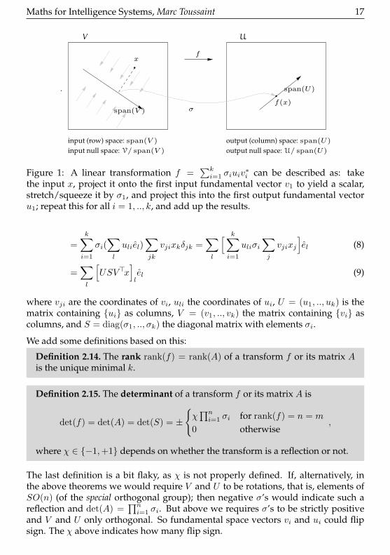
Figure 1: A linear transformation f =∑ki=1 σiuiv
∗i can be described as: take
the input x, project it onto the first input fundamental vector v1 to yield a scalar,stretch/squeeze it by σ1, and project this into the first output fundamental vectoru1; repeat this for all i = 1, .., k, and add up the results.
=
k∑i=1
σi(∑l
uliel)∑jk
vjixkδjk =∑l
[ k∑i=1
uliσi∑j
vjixj
]el (8)
=∑l
[USV>x
]lel (9)
where vji are the coordinates of vi, uli the coordinates of ui, U = (u1, .., uk) is thematrix containing ui as columns, V = (v1, .., vk) the matrix containing vi ascolumns, and S = diag(σ1, .., σk) the diagonal matrix with elements σi.
We add some definitions based on this:
Definition 2.14. The rank rank(f) = rank(A) of a transform f or its matrix Ais the unique minimal k.
Definition 2.15. The determinant of a transform f or its matrix A is
det(f) = det(A) = det(S) = ±
χ∏ni=1 σi for rank(f) = n = m
0 otherwise,
where χ ∈ −1,+1 depends on whether the transform is a reflection or not.
The last definition is a bit flaky, as χ is not properly defined. If, alternatively, inthe above theorems we would require V and U to be rotations, that is, elements ofSO(n) (of the special orthogonal group); then negative σ’s would indicate such areflection and det(A) =
∏ni=1 σi. But above we requires σ’s to be strictly positive
and V and U only orthogonal. So fundamental space vectors vi and ui could flipsign. The χ above indicates how many flip sign.

18 Maths for Intelligence Systems, Marc Toussaint
Definition 2.16. a) The row space (also called right (=input) fundamental space)of a transform f is spanvirank(f)
i=1 . The input null space (or right null space)V⊥ is the subspace orthogonal to the row space, such that v ∈ V⊥ ⇒ f(v) = 0.
b) The column space or (also called left (=output) fundamental space) of atransform f is spanuirank(f)
i=1 . The output null space (or left null space) U⊥the subspace orthogonal to the column space, such that u ∈ U⊥ ⇒ 〈f(·), u〉 = 0.
2.5 Point of departure from the coordinate-free notation
The coordinate-free introduction of vectors and transforms helps a lot to under-stand what these fundamentally are. That coordinate vectors and matrices are ’just’coordinates and rely on a choice of basis; what a metric gij really is; that only for aEuclidean metric the inner product satisfies 〈v, w〉 = v>w. Further, the coordinate-free view is essential to understand that vector coordinates behave differently to1-form coordinates (e.g., “gradients”!) under a transformation of the basis. Wepostpone this discussion of contra- versus covariance.
However, we now understood that columns correspond vectors, rows to 1-forms,and in the Euclidean case the 1-form v∗ directly corresponds to v>, in the non-Euclidean to v>G. In applications we typically represent things from start in or-thonormal bases (including perhaps non-Euclidean metrics), there is not much gainsticking to the coordinate-free notation in most cases. Only when the matrix nota-tion gets confusing (and this happens, e.g. when trying to compute something likethe “Jacobian of a Jacobian”, or applying the chain and product rule for a matrixexpression ∂xf(x)>A(x)b(x)) it is always a save harbour to remind what we actuallytalk about.
Therefore, in the rest of the notes we rely on the normal coordinate-based view.Only in some explanations we remind on the coordinate-free view when helpful.
2.6 Filling SVD with life
In the following we list some statements—all of them relate to the SVD theoremand together they’re meant to give a more intuitive understanding of the equationA =
∑ki=1 σiuiv
>i = USV>.
2.6.1 Understand vv> as projection
• The projection of a vector x ∈ V onto a vector v ∈ V, is given by
x‖ =1
v2v〈v, x〉 or
1
v2vv>x .
Maths for Intelligence Systems, Marc Toussaint 19
Here, the 1v2 is normalizing in case v does not have length |v| = 1.
• The projection-on-v-matrix vv> is symmetric, semi-pos-def, and has rank(vv>) =1.
• The projection of a vector x ∈ V onto a subvector space spanviki=1 for or-thonormal viki=1 is given by
x‖ =∑i
viv>ix = V V Tx
where V = (v1, .., vk) ∈ Rn×k.
• The projection matrix V V> for orthonormal V is symmetric, semi-pos-def,and has rank(V V>) = k.
2.6.2 SVD for symmetric matrices
• Thm 2⇒ Every symmetric matrix A is of the form
A =∑i
λiviv>i = V ΛV>
for orthonormal V = (v1, .., vk). Here λi = ±σi and Λ = diag(λ) is the diag-onal matrix of λ’s. This describes nothing but a stretching/squeezing alongorthogonal projections.
• The λi and vi are also the eigenvalues and eigenvectors of A, that is, for alli = 1, .., k:
Avi = λivi .
The SVD A = V SV>= V SV -1 is therefore also the eigendecomposition of A.
• The pseudo-inverse of a symmetric matrix is
A† =∑i
λ-1i viv
>i = V S-1V>
which simply does the reverse stretching/squeezing along the same orthog-onal projections. Note that
AA† = A†A = V V>
is the projection on viki=1. For rank(A) = n we have V V>= I and A† = A-1.For rank(A) < n, we have that A†y minimizes minx ||Ax − y||2, but there areinfinitly many x’s that minimize this, spanned by the null space of A. A†y isthe minimizer closest to zero (with smallest norm).
20 Maths for Intelligence Systems, Marc Toussaint
• Consider a data set D = ximi=1, xi ∈ Rn. For simplicity assume it has zeromean,
∑mi=1 xi = 0. The covariance matrix is defined as
C =1
n
∑i
xix>i =
1
nX>X
where (consistent to ML lecture convention) the data matrix X containes x>iin the ith row. Each xix
>i is a projection. C is symmetric and semi-pos-dev.
Using SVD we can write
C =∑i
λiviv>i
and λi is the data variance along the eigenvector vi;√λi the standard devia-
tion along vi; and√λivi the principle axis vectors that make the ellipsoid we
typically illustrate convariances with.
2.6.3 SVD for general matrices
• For rank(A) = n, the determinant of a matrix is det(A) =∏i σi. We may
define the volume spanned by any bini=1 as
vol(bini=1) = det(B) , B = (b1, .., bn) ∈ Rn×n .
It follows thatvol(Abini=1) = det(A) det(B)
that is, the volume is being multiplied with det(A) =∏i σi, which is consis-
tent with our understanding of transforms as stretchings/squeezings alongprojections.
• The pseudo-inverse of a general matrix is
A† =∑i
σ-1i viu
>i = V S-1U> .
If k = n (full input rank), rank(A>A) = n and
(A>A)-1A>= (V SU>USV>)-1V SU>= V −>S−2V -1V SU>= V S-1U>= A†
and A† is also called left pseudoinverse because A†A = In.
If k = m (full output rank), rank(AA>) = m and
A>(AA>)-1 = V SU>(USV>V SU>)-1 = V SU>U−>S−2U -1 = V S-1U>= A†
and A† is also called right pseudoinverse because AA† = Im.

Maths for Intelligence Systems, Marc Toussaint 21
• Assume m = n (same input/output dimension, or V = U), but k < n. Thenthere exist orthogonal V,U ∈ Rn×n such that
A = UDV> , D = diag(σ1, .., σk, 0, .., 0) =S 0
0 0
.
Here, V and U contain a full orthonormal basis instead of only k orthonormalvectors. But the diagonal matrix D projects all but k of those to zero. Everysquare matrix A ∈ Rn×n can be written like this.
Definition 2.17 (Rotation). Given a scalar-product 〈·, ·〉 on V, a linear transformf : V → V is called rotation iff it preserves the scalar product, that is,
∀v, w ∈ V : 〈f(v), f(w)〉 = 〈v, w〉 . (10)
• Every rotation matrix is orthogonal, i.e., composed of columns of orthonor-mal vectors.
• Every rotation has rank n and σ1,..,n = 1. (No stretching/squeezing.)
• Every square matrix can be written asrotationU · scalingD · rotationV -1
2.7 Eigendecomposition
Definition 2.18. The diagonalization or eigendecomposition of a square ma-trix A ∈ Rn×n is (if it exists!)
A = QΛQ-1
where Λ = diag(λ1, .., λn) is a diagonal matrix of eigenvalues. Each column qiof Q is an eigenvector.
• The set of eigenvalues is the set of roots of the characteristic polynomialpA(λ) = det(λI − A). Why? Because then A − λI has ’volume’ zero (orrank < n), showing that one vector is mapped to zero, that is 0 = (A−λI)x =Ax− λx.
• Is every square matrix diagonalizable? No, but only an n2 − 1-dimensionalsubset of matrices are not diagonalizable; most matrices are. A matrix is notdiagonalizable if an eigenvalue λ has multiplicity k (more precisely, λ is a rootof pA(λ) with multiplicity k), but n− rank(A− λI) (the dimensionality of thespan of the eigenvectors of λ!) is less than k. Therefore, the eigenvectors of λare not linearly independent; they do not span the necessary k dimensions.
So, only very “special” matrices are not diagonalizable. Random matrices are(with prob 1).

22 Maths for Intelligence Systems, Marc Toussaint
• Symmetric matrices? → SVD
• Rotations? Not real. But complex! Think of oscillating projection onto eigen-vector. If φ is the rotation angle, e±iφ are eigenvalues.
2.7.1 Power Method
To find the largest eigenvector of A, initialize x randomly and iterate
x← Ax , x← 1
||x||x
– If this converges, x must be an eigenvector and λ = x>Ax the eigenvalue.
– IfA is diagonalizable, and x is initially a non-zero linear combination of all eigen vectors,then it is obvious that x will converge to the “largest” (in absolute terms |λi|) eigenvector(=eigenvector with largest eigenvalue). Actually, if the largest (by norm) eigenvector isnegative, then it doesn’t really converge by flip sign at every iteration.
2.7.2 Power Method including the smallest eigenvalue
A trick, hard to find in the literature, to also compute the smallest eigenvalue and-vector is the following. We assume all eigenvalues to be positive. Initialize x andy randomly, iterate
x← Ax , λ← ||x|| , x← x/λ , y ← (λI −A)y , y ← y/||y||
Then y will converge to the smallest eigenvector, and λ− ||y||will be its eigenvalue.Note that (in the limit) A − λI only has negative eigenvalues, therefore ||y|| shouldbe positive. Finding smallest eigenvalues is a common problem in model fitting.
2.7.3 Why should I care about Eigenvalues and Eigenvectors?
– Least squares problems (finding smallest eigenvalue/-vector); (e.g. Camera Calibration,Bundle Adjustment, Plane Fitting)
– PCA
– stationary distributiuons of Markov Processes
– Page Rank
– Spectral Clustering
– Spectral Learning (e.g., as approach to training HMMs)
Maths for Intelligence Systems, Marc Toussaint 23
2.8 Point of Departure: Numerics to compute these things
We will not go into details of numerics. Nathan’s script gives a really nice explaina-tion of the QR-method. I just mention two things:
(i) The most important forms of matrices for numerics are diagonal matrices, or-thogonal matrices, and upper triangular matrices. One reason is that all three typescan very easily be inverted. A lot of numerics is about finding decompositions ofgeneral matrices into products of these special-form matrices, e.g.:
– QR-decomposition: A = QR with Q orthogonal and R upper triangular.
– LU-decomposition: A = LU with U and L>upper triangular.
– Cholesky decomposition: (symmetric) A = C>C with C upper triangular
– Eigen- & singular value decompositions
Often, these decompositions are intermediate steps to compute eigenvalue or sin-gular value decompositions.
(ii) Use linear algebra packages. At the origin of all is LAPACK; browse throughhttp://www.netlib.org/lapack/lug/ to get an impression of what reallyhas been one of the most important algorithms in all technical areas of the last halfcentury. Modern wrappers are: Matlab (Octave), which originated as just a consoleinterface to LAPACK; the C++-library Eigen; or the Python NumPy.
2.9 Examples and Exercises
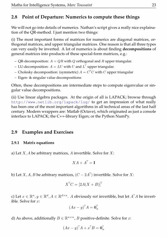
2.9.1 Matrix equations
a) Let X,A be arbitrary matrices, A invertible. Solve for X :
XA+A>= I
b) Let X,A,B be arbitrary matrices, (C − 2A>) invertible. Solve for X :
X>C = [2A(X +B)]>
c) Let x ∈ Rn, y ∈ Rd, A ∈ Rd×n. A obviously not invertible, but let A>A be invert-ible. Solve for x:
(Ax− y)>A = 0>n
d) As above, additionally B ∈ Rn×n, B positive-definite. Solve for x:
(Ax− y)>A+ x>B = 0>n

24 Maths for Intelligence Systems, Marc Toussaint
2.9.2 Examples for Vector Spaces (voluntary, discussed on Oct 23rd)
(i) Find 3 interesting examples of vector spaces that we haven’t covered in class.What are their dimensions? What bases are commonly used to representthem? (It’s okay to look this up in a textbook or online—just find interest-ing examples.)
(ii) Come up with one example of a set which is almost a vector space, i.e. it satis-fies some of the core requirements of a vector space, but not all.
2.9.3 Basis
Given a linear transform f : R2 → R2,
f(x) = Ax =7 −105 −8
x .
Consider the basis B =1
1
,21
, which we also simply refer to by the matrix
B =1 21 1
. Given a vector x in the vector space R2, we denote its coordinates in
basis B with xB .
(i) Show that x = BxB .
(ii) What is the matrix FB of f in the basis B, i.e., such that [f(x)]B = FBxB?Prove the general equation FB = B-1AB.
(iii) Provide FB numerically
Note that for a matrix M =a bc d
, M -1 = 1ad−bc
d −b−c a
2.9.4 From the Robotics Course (voluntary)
You have a book lying on the table. The edges of the book define the basis B, theedges of the table define basis A. Initially A and B are identical (also their originsalign). Now we rotate the book by 45 counter-clock-wise about its origin.
(i) Given a dot p marked on the book at position pB = (1, 1) in the book coordi-nate frame, what are the coordinates pA of that dot with respect to the tableframe?
(ii) Given a point x with coordinates xA = (0, 1) in table frame, what are itscoordinates xB in the book frame?
(iii) What is the coordinate transformation matrix from book frame to table frame,and from table frame to book frame?
Maths for Intelligence Systems, Marc Toussaint 25
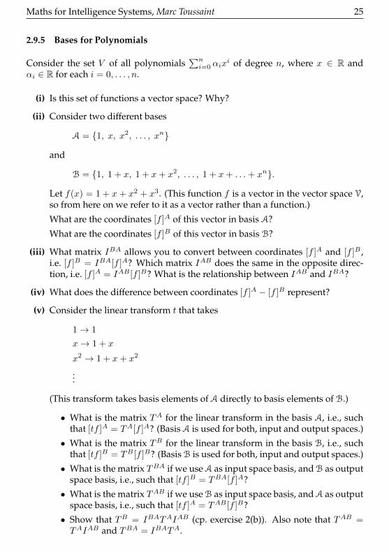
2.9.5 Bases for Polynomials
Consider the set V of all polynomials∑ni=0 αix
i of degree n, where x ∈ R andαi ∈ R for each i = 0, . . . , n.
(i) Is this set of functions a vector space? Why?
(ii) Consider two different bases
A = 1, x, x2, . . . , xn
and
B = 1, 1 + x, 1 + x+ x2, . . . , 1 + x+ . . .+ xn.
Let f(x) = 1 + x+ x2 + x3. (This function f is a vector in the vector space V,so from here on we refer to it as a vector rather than a function.)
What are the coordinates [f ]A of this vector in basis A?
What are the coordinates [f ]B of this vector in basis B?
(iii) What matrix IBA allows you to convert between coordinates [f ]A and [f ]B ,i.e. [f ]B = IBA[f ]A? Which matrix IAB does the same in the opposite direc-tion, i.e. [f ]A = IAB [f ]B? What is the relationship between IAB and IBA?
(iv) What does the difference between coordinates [f ]A − [f ]B represent?
(v) Consider the linear transform t that takes
1→ 1
x→ 1 + x
x2 → 1 + x+ x2
...
(This transform takes basis elements of A directly to basis elements of B.)
• What is the matrix TA for the linear transform in the basis A, i.e., suchthat [tf ]A = TA[f ]A? (Basis A is used for both, input and output spaces.)
• What is the matrix TB for the linear transform in the basis B, i.e., suchthat [tf ]B = TB [f ]B? (Basis B is used for both, input and output spaces.)
• What is the matrix TBA if we use A as input space basis, and B as outputspace basis, i.e., such that [tf ]B = TBA[f ]A?
• What is the matrix TAB if we use B as input space basis, and A as outputspace basis, i.e., such that [tf ]A = TAB [f ]B?
• Show that TB = IBATAIAB (cp. exercise 2(b)). Also note that TAB =TAIAB and TBA = IBATA.

26 Maths for Intelligence Systems, Marc Toussaint
2.9.6 Projections
(i) In Rn, a plane (through the origin) is typically described by the linear equa-tion
c>x = 0 , (11)
where c ∈ Rn parameterizes the plane. Provide the matrix that describesthe orthogonal projection onto this plane. (Tip: The SVD describes matricesas sum of rank-1 matrices; here, think of the projection as I minus a rank-1matrix.)
(ii) In Rn, let’s have k linearly independent viki=1, which form the matrix V =(x1, .., xk) ∈ Rn×k. Let’s formulate a projection using an optimality principle,namely,
α∗(x) = argminα∈Rk
||x− V α||2 . (12)
Note that V α =∑ki=1 αivi is just the linear combination of v’s with coeffi-
cients α. The projection of a vector x is then
x|| = V α∗(x) . (13)
Derive the equation for the optimal α∗(x) from the optimality principle.
2.9.7 SVD
Consider the matrices
A =
1 0 0
0 −2 0
0 0 0
0 0 0
, B =
1 1 1
1 0 −1
2 1 0
0 1 2
(14)
(i) Describe their 4 fundamental spaces (dimentionality, possible basis vectors).
(ii) Find the SVD of A (using pen and paper only!)
(iii) Given an arbitrary input vector x ∈ R3, write the linear transformations PAand PB which extract its “input null space” component for each respectivematrix.
(iv) Compute the pseudo inverse A†.
(v) Determine all solutions to the linear equations Ax = y and Bx = y withy = (2, 3, 0, 0). What is the more general expression for an arbitrary y?

Maths for Intelligence Systems, Marc Toussaint 27
2.9.8 Covariance and PCA
Suppose we’re given a collection of zero-centered data points D = xiNi=1, witheach xi ∈ Rn. The covariance matrix is defined as
C =1
n
N∑i=1
xix>i =
1
nX>X
where (consistent to ML lecture convention) the data matrix X = (x>1; ..;x>N ) con-tains each x>i as rows, X>= (x1, .., xN ).
If we project D onto some unit vector v ∈ Rn, then the variance of the projecteddata points is v>Cv. Show that the direction that maximizes this variance is thelargest eigenvector of C. (Hint: Expand v n terms of the eigenvector basis of C andexploit the constraint v>v = 1.)
(This optimization is the first step of the so-called Principal Components Analysis(PCA).)
2.9.9 Bonus: Scalar product and Orthogonality
(i) Show that f(x, y) = 2x1y1 − x1y2 − x2y1 + 5x2y2 is an scalar product on R2.
(ii) In the space of functions with the scalar product 〈fg〉 =∫∞−∞ f(x)g(x)dx, what
is the projection of sin(x) onto sin(2x)? (Graphical argument is ok)
(iii) What property does a matrix M has to satisfy in order to be a valid metrictensor, i.e. such that x>My is a valid scalar product?
2.9.10 Eigenvectors
(i) A symmetric matrix A ∈ Rn×n is called positive semidefinite (PSD) if x>Ax ≥0,∀x ∈ Rn. (PSD is usually only used with symmetric matrices.) Show thatall eigenvalues of a PSD matrix are non-negative.
(ii) Show that if v is an eigenvector ofAwith eigenvalue λ, then v is also an eigen-vector ofAk for any positive integer k. What is the corresponding eigenvalue?
(iii) Let v be an eigenvector of A with eigenvalue λ and w an eigenvector of A>
with a different eigenvalue µ 6= λ. Show that v and w are orthogonal withrespect to the dot product.
(iv) Suppose A ∈ Rn×n has eigenvalues λ1, . . . , λn ∈ R. What are the eigenvaluesof A+ αI for α ∈ R and I an identity matrix?
28 Maths for Intelligence Systems, Marc Toussaint
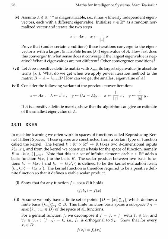
(v) Assume A ∈ Rn×n is diagonalizable, i.e., it has n linearly independent eigen-vectors, each with a different eigenvalue. Initialize x ∈ Rn as a random nor-malized vector and iterate the two steps
x← Ax , x← 1
||x||x
Prove that (under certain conditions) these iterations converge to the eigen-vector x with a largest (in absolute terms |λi|) eigenvalue of A. How fast doesthis converge? In what sense does it converge if the largest eigenvalue is neg-ative? What if eigenvalues are not different? Other convergence conditions?
(vi) LetA be a positive definite matrix with λmax its largest eigenvalue (in absoluteterms |λi|). What do we get when we apply power iteration method to thematrix B = A− λmaxI? How can we get the smallest eigenvalue of A?
(vii) Consider the following variant of the previous power iteration:
z ← Ax , λ← x>z , y ← (λI −A)y , x← 1
||z||z , y ← 1
||y||y .
IfA is a positive definite matrix, show that the algorithm can give an estimateof the smallest eigenvalue of A.
2.9.11 RKHS
In machine learning we often work in spaces of functions called Reproducing Ker-nel Hilbert Spaces. These spaces are constructed from a certain type of functioncalled the kernel. The kernel k : Rd × Rd → R takes two d-dimensional inputsk(x, x′), and from the kernel we construct a basis for the space of function, namelyB = k(x, ·)x∈Rd . Note that this is a set of infinite element: each x ∈ Rd adds abasis function k(x, ·) to the basis B. The scalar product between two basis func-tions kx = k(x, ·) and kx′ = k(x′, ·) is defined to be the kernel evaluation itself:〈kx, kx′〉 = k(x, x′). The kernel function is therefore required to be a positive defi-nite function so that it defines a viable scalar product.
(i) Show that for any function f ∈ spanB it holds
〈f, kx〉 = f(x)
(ii) Assume we only have a finite set of points D = xini=1, which defines afinite basis kxini=1 ⊂ B. This finite function basis spans a subspace FD =spankxi : xi ∈ D of the space of all functions.
For a general function f , we decompose it f = fs + f⊥ with fs ∈ FD and∀g ∈ FD : 〈f⊥, g〉 = 0, i.e., f⊥ is orthogonal to FD. Show that for everyxi ∈ D:
f(xi) = fs(xi)

Maths for Intelligence Systems, Marc Toussaint 29
(Note: This shows that the function values of any function f at the data pointsD only depend on the part fs which is inside the spann of kxi : xi ∈ D. Thisimplies the so-called representer theorem, which is fundamental in kernelmachines: A loss can only depend on function values f(xi) at data points,and therefore on fs. The part f⊥ can only increase the complexity (norm) ofa function. Therefore, the simplest function to optimize any loss will havef⊥ = 0 and be within spankxi : xi ∈ D.)
(iii) Within spankxi : xi ∈ D, what is the coordinate representation of the scalarproduct?
3 Derivatives
3.1 The coordinate-free view: The meaning of life for a derivativeis to eat a vector and output a scalar
We briefly state the general concept of a derivative in coordinate-free form. Practi-tioners may skip this.
Definition 3.1. Given a function f : V → G we define the differential
df∣∣x
: V → G, v 7→ limh→0
f(x+ hv)− f(x)
h
This definition holds whenever G is a continuous space that allows the definitionof this limit and the limit exists (f is differentiable). The notation df |x reads “thedifferential at location x”, i.e., evaluating this derivative at location x.
Note that df |x is a mapping from a “tangent vector” v to output-change. Further,by this definition df |x is linear. Therefore df |x is a G-valued 1-form. As discussedearlier, we can introduce coordinates for 1-forms; these coordinates are what typi-cally called is the “gradient” or “Jacobian”. But here we explicitly see that we speakof coordinates of a 1-form.
3.2 Don’t confuse partial and total derivative
3.2.1 Partial derivative
In coordinates, we may think of a function f : Rn → R simply as a function of narguments, f(x1, .., xn).
Definition 3.2. The partial derivative of a function of multiple arguments f(x1, .., xn)
30 Maths for Intelligence Systems, Marc Toussaint
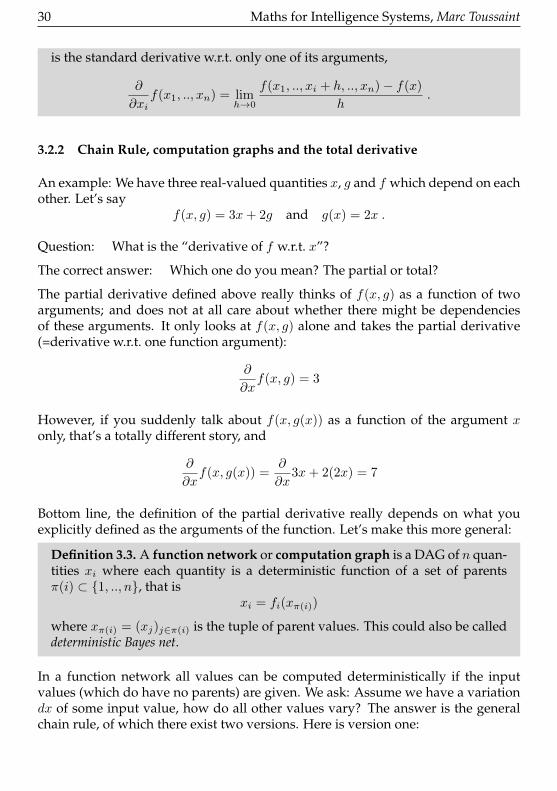
is the standard derivative w.r.t. only one of its arguments,
∂
∂xif(x1, .., xn) = lim
h→0
f(x1, .., xi + h, .., xn)− f(x)
h.
3.2.2 Chain Rule, computation graphs and the total derivative
An example: We have three real-valued quantities x, g and f which depend on eachother. Let’s say
f(x, g) = 3x+ 2g and g(x) = 2x .
Question: What is the “derivative of f w.r.t. x”?
The correct answer: Which one do you mean? The partial or total?
The partial derivative defined above really thinks of f(x, g) as a function of twoarguments; and does not at all care about whether there might be dependenciesof these arguments. It only looks at f(x, g) alone and takes the partial derivative(=derivative w.r.t. one function argument):
∂
∂xf(x, g) = 3
However, if you suddenly talk about f(x, g(x)) as a function of the argument xonly, that’s a totally different story, and
∂
∂xf(x, g(x)) =
∂
∂x3x+ 2(2x) = 7
Bottom line, the definition of the partial derivative really depends on what youexplicitly defined as the arguments of the function. Let’s make this more general:
Definition 3.3. A function network or computation graph is a DAG of n quan-tities xi where each quantity is a deterministic function of a set of parentsπ(i) ⊂ 1, .., n, that is
xi = fi(xπ(i))
where xπ(i) = (xj)j∈π(i) is the tuple of parent values. This could also be calleddeterministic Bayes net.
In a function network all values can be computed deterministically if the inputvalues (which do have no parents) are given. We ask: Assume we have a variationdx of some input value, how do all other values vary? The answer is the generalchain rule, of which there exist two versions. Here is version one:
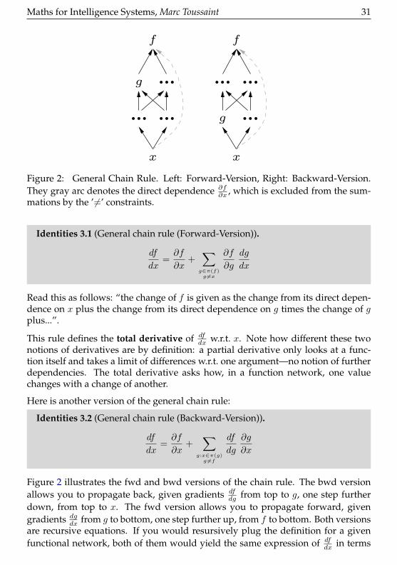
Maths for Intelligence Systems, Marc Toussaint 31
ff
g
x
g
x
Figure 2: General Chain Rule. Left: Forward-Version, Right: Backward-Version.They gray arc denotes the direct dependence ∂f
∂x , which is excluded from the sum-mations by the ’6=’ constraints.
Identities 3.1 (General chain rule (Forward-Version)).
df
dx=∂f
∂x+∑g∈π(f)g 6=x
∂f
∂g
dg
dx
Read this as follows: “the change of f is given as the change from its direct depen-dence on x plus the change from its direct dependence on g times the change of gplus...”.
This rule defines the total derivative of dfdx w.r.t. x. Note how different these two
notions of derivatives are by definition: a partial derivative only looks at a func-tion itself and takes a limit of differences w.r.t. one argument—no notion of furtherdependencies. The total derivative asks how, in a function network, one valuechanges with a change of another.
Here is another version of the general chain rule:
Identities 3.2 (General chain rule (Backward-Version)).
df
dx=∂f
∂x+
∑g:x∈π(g)g 6=f
df
dg
∂g
∂x
Figure 2 illustrates the fwd and bwd versions of the chain rule. The bwd versionallows you to propagate back, given gradients df
dg from top to g, one step furtherdown, from top to x. The fwd version allows you to propagate forward, givengradients dg
dx from g to bottom, one step further up, from f to bottom. Both versionsare recursive equations. If you would resursively plug the definition for a givenfunctional network, both of them would yield the same expression of df
dx in terms

32 Maths for Intelligence Systems, Marc Toussaint
of partial derivatives only.
Let’s compare to the chain rule as it is usually given (written more precisely),
∂f(g(x))
∂x=∂f(g)
∂g
∣∣∣∣g=g(x)
∂g(x)
∂x
Note that we here very explicitly notated that ∂f(g)∂g considers f to be a function of
the argument g, which is evaluted at g = g(x). Written like this, the rule is fine.But the above discussion and explicitly distinguishing between partial and totalderivative is, when things get complicated, less prone to confusion.
3.3 Gradient, Jacobian, Hessian, Taylor Expansion
3.3.1 Gradient, Jacobian, and Hessian
Lets focus again on functions f : Rn → Rd
Definition 3.4. Given f : Rn → Rd, we define the derivative (also called Jaco-bian matrix) as
∂
∂xf(x) =
∂∂x1
f1(x) ∂∂x2
f1(x) . . . ∂∂xn
f1(x)∂∂x1
f2(x) ∂∂x2
f2(x) . . . ∂∂xn
f2(x)...
...∂∂x1
fd(x) ∂∂x2
fd(x) . . . ∂∂xn
fd(x)
Consistent with this, we also define the derivative of f : Rn → R1 as the rowvector of partial derivatives
∂
∂xf(x) = (
∂
∂x1f, ..,
∂
∂xnf) .
Further, we define the gradient as the corresponding column “vector”
∇f(x) =[ ∂∂xf(x)
]>.
The “purpose” of a derivative is to output a change of function value when beingmultiplied to a change of input δ. That is, in first order approximation, we have
f(x+ δ)− f(x) = ∂f(x) δ .
This equation holds, no matter if the output space is Rd or R. In the gradient nota-tion we have
f(x+ δ)− f(x) = ∇f(x)>δ .

Maths for Intelligence Systems, Marc Toussaint 33
Note that this latter equation is truly independent of the choice of vector space ba-sis and independent of an optional metric or scalar product in V : This transposeshould not be understood as a scalar product between two vectors, but rather asundoing the transpose in the definition of ∇f . As mentioned earlier, all this is con-sistent to understanding these derivatives as coordinates of a 1-form.
In the abstract, coordinate-free notation, the second derivative would be defined asthe 2-form
d2f∣∣x
: V × V → G, (15)
(v, w) 7→ limh→0
df∣∣x+hw
(v)− f∣∣x(v)
h(16)
= limh,l→0
f(x+ hw + lv)− f(x+ hw)− f(x+ lv) + f(x)
hl(17)
Definition 3.5. In coordinates, we define the Hessian of a scalar function f :Rn → R as the symmetric matrix
∇2f(x) =∂
∂x∇f(x) =
∂2
∂x1∂x1f ∂2
∂x1∂x2f . . . ∂2
∂x1∂xnf
∂2
∂x2∂x1f ∂2
∂x2∂x2f . . . ∂2
∂x2∂xnf
......
∂2
∂xn∂x1f ∂2
∂xn∂x2f . . . ∂2
∂xn∂xnf
The Hessian can be thought of as the coordinates of the 2-form defined above(which would actually be a row vector of row vectors), or as the Jacobian of ∇f .Using the Hessian, we can express the 2nd order approximation of f as:
f(x+ δ) = f(x) + ∂f(x) δ +1
2δ>∇2f(x) δ .
As a Hessian H is symmetric we can decompose it as H =∑i λihih
>i with eigen-
values λi and eigenvectors hi.
λi gives the curvature (as in the normal 1D 2nd derivative) along an eigenvectorhi. If λi > 0, f is convex along hi; if λi < 0, f is concave along hi. If some λi’s arepositive, some negative, and we are at a zero-gradient point ∂xf = 0, this is calleda saddle point.
3.3.2 Taylor expansion
In 1D, we have
f(x+ v) ≈ f(x) + f ′(x)v +1
2f ′′(x)v2 + · · ·+ 1
k!f (k)(x)vk (18)

34 Maths for Intelligence Systems, Marc Toussaint
For f : Rn → R, we have
f(x+ v) ≈ f(x) +∇f(x)>v +1
2v>∇2f(x)v + · · · (19)
which is equivalent to
f(x+ v) ≈ f(x) +∑j
∂
∂xjf(x)vj +
1
2
∑jk
∂2
∂xj∂xkf(x)vjvk + · · · (20)
3.4 Contra- and co-variance
In Section 2.2.6 we summarized the effects of a coorindate transformation. We recapthe same here again also for derivatives and scalar products.
We have a vector space V , and a function f : V → R. We’ll be interested in thechange of function value df |x(δ) for change of input δ ∈ V , as well as the value ofthe scalar product 〈δ, δ〉. All these quantities are defined without any reference tocoordinates; we’ll check now how their coordinate representations change with achange of basis.
As in Section 2.2.6 we have two bases A = (a1, .., an) and B = (b1, .., bn), and thetransformation T that maps each ai to bi, i.e., B = TA. Given a vector δ we denoteits coordinates in A by [δ]A, and its coordinates in B by [δ]B . Let TAA = B bethe matrix representation of T in the old A coordinates (B contains the new basisvectors b as columns).
• We previously learned that[δ]A = B[δ]B
that is, the matrix B carries new coordinates to old ones. These coordinatesare said to be contra-variant: they transform ‘against’ the transformation ofthe basis vectors.
• We require thatdf |x(δ) = [∂xf ]A[δ]A = [∂xf ]B [δ]B
must be invariant, i.e., the change of function value for δ should not dependon whether we compute it using A or B coordinates. It follows
[∂xf ]A[δ]A = [∂xf ]AB[δ]B = [∂xf ]B [δ]B (21)
[∂xf ]AB = [∂xf ]B (22)
that is, the matrixB carries old 1-form-coordinates to new 1-form-coordinates.Therefore, such 1-form-coordinates are called co-variant: they transform ‘with’the transformation of basis vectors.

Maths for Intelligence Systems, Marc Toussaint 35
• What we just wrote for the derivative df |x(δ) we could equally write andargue for any 1-form v∗ ∈ V ∗; we always require that the value v∗(δ) is in-variant.
• We also require that the scalar product 〈δ, δ〉 is invariant. Let
〈δ, δ〉 = [δ]A>[G]A[δ]A = [δ]B>[G]B [δ]B
where [G]A and [G]B are the 2-form-coordinates (metric tensor) in the old andnew basis. It follows
[δ]A>[G]A[δ]A = [δ]B>B>[G]AB[δ]B (23)
[G]B = B>[G]AB (24)
that is, the matrix carries the old 2-form-coordinates to new ones. These coor-dinates are called twice co-variant.
Consider the following example: We have the function f : R2 → R, f(x) = x1 + x2.The function’s partial derivative is of course ∂f
∂x = (1 1). Now let’s transformthe coordinates of the space: we introduce new coordinates (z1, z2) = (2x1, x2) or
z = B-1x with B = 1
2 00 1
. The same function, written in the new coordinates, is
f(z) = 12z1 + z2. The partial derivatives of that same function, written in these new
coordinates, is ∂f∂z = ( 1
2 1).
Generally, consider we have two kinds of mathematical objects and when we mul-tiply them together this gives us a scalar. The scalar shouldn’t depend on anychoice of coordinate system and is therefore invariant against coordinate trans-forms. Then, if one of the objects transforms in a covariant (“transforming withthe transformation”) manner, the other object must transform in a contra-variant(“transforming contrary to the transformation”) manner to ensure that the resultingscalar is invariant. This is a general principle: whenever two things multiply to-gether to give an invariant thing, one should transform co- the other contra-variant.
Let’s also check Wikipedia:
– “For a vector to be basis-independent, the components [=coordinates] of the vector mustcontra-vary with a change of basis to compensate. That is, the matrix that transformsthe vector of components must be the inverse of the matrix that transforms the basisvectors. The components of vectors (as opposed to those of dual vectors) are said to becontravariant.
– For a dual vector (also called a covector) to be basis-independent, the components ofthe dual vector must co-vary with a change of basis to remain representing the samecovector. That is, the components must be transformed by the same matrix as the changeof basis matrix. The components of dual vectors (as opposed to those of vectors) are saidto be covariant.”
Ordinary gradient descent of the form x← x+α∇f adds objects of different types:contra-variant coordinates x with co-variant partial derivatives∇f . Clearly, adding
36 Maths for Intelligence Systems, Marc Toussaint
two such different types leads to an object who’s transformation under coordinatetransforms is strange—and indeed the ordinary gradient descent is not invariantunder transformations.
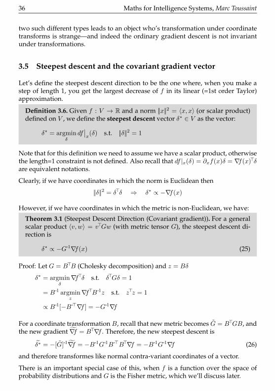
3.5 Steepest descent and the covariant gradient vector
Let’s define the steepest descent direction to be the one where, when you make astep of length 1, you get the largest decrease of f in its linear (=1st order Taylor)approximation.
Definition 3.6. Given f : V → R and a norm ||x||2 = 〈x, x〉 (or scalar product)defined on V , we define the steepest descent vector δ∗ ∈ V as the vector:
δ∗ = argminδ
df∣∣x(δ) s.t. ||δ||2 = 1
Note that for this definition we need to assume we have a scalar product, otherwisethe length=1 constraint is not defined. Also recall that df |x(δ) = ∂xf(x)δ = ∇f(x)>δare equivalent notations.
Clearly, if we have coordinates in which the norm is Euclidean then
||δ||2 = δ>δ ⇒ δ∗ ∝ −∇f(x)
However, if we have coordinates in which the metric is non-Euclidean, we have:
Theorem 3.1 (Steepest Descent Direction (Covariant gradient)). For a generalscalar product 〈v, w〉 = v>Gw (with metric tensor G), the steepest descent di-rection is
δ∗ ∝ −G-1∇f(x) (25)
Proof: Let G = B>B (Cholesky decomposition) and z = Bδ
δ∗ = argminδ∇f>δ s.t. δ>Gδ = 1
= B-1 argminz∇f>B-1z s.t. z>z = 1
∝ B-1[−B->∇f ] = −G-1∇f
For a coordinate transformation B, recall that new metric becomes G = B>GB, andthe new gradient ∇f = B>∇f . Therefore, the new steepest descent is
δ∗ = −[G]-1∇f = −B-1G-1B->B>∇f = −B-1G-1∇f (26)
and therefore transformes like normal contra-variant coordinates of a vector.
There is an important special case of this, when f is a function over the space ofprobability distributions and G is the Fisher metric, which we’ll discuss later.
Maths for Intelligence Systems, Marc Toussaint 37
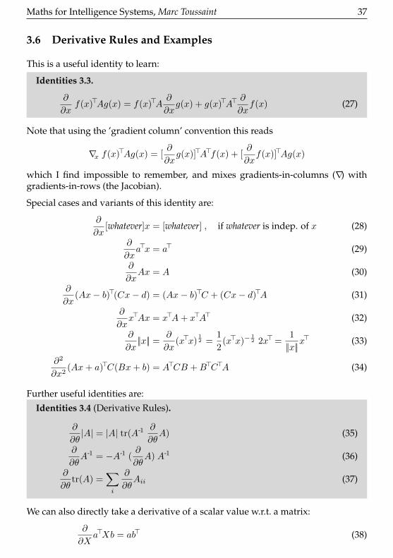
3.6 Derivative Rules and Examples
This is a useful identity to learn:
Identities 3.3.
∂
∂xf(x)>Ag(x) = f(x)>A
∂
∂xg(x) + g(x)>A>
∂
∂xf(x) (27)
Note that using the ’gradient column’ convention this reads
∇x f(x)>Ag(x) = [∂
∂xg(x)]>A>f(x) + [
∂
∂xf(x)]>Ag(x)
which I find impossible to remember, and mixes gradients-in-columns (∇) withgradients-in-rows (the Jacobian).
Special cases and variants of this identity are:
∂
∂x[whatever]x = [whatever] , if whatever is indep. of x (28)
∂
∂xa>x = a> (29)
∂
∂xAx = A (30)
∂
∂x(Ax− b)>(Cx− d) = (Ax− b)>C + (Cx− d)>A (31)
∂
∂xx>Ax = x>A+ x>A> (32)
∂
∂x||x|| = ∂
∂x(x>x)
12 =
1
2(x>x)−
12 2x>=
1
||x||x> (33)
∂2
∂x2(Ax+ a)>C(Bx+ b) = A>CB +B>C>A (34)
Further useful identities are:
Identities 3.4 (Derivative Rules).
∂
∂θ|A| = |A| tr(A-1 ∂
∂θA) (35)
∂
∂θA-1 = −A-1 (
∂
∂θA) A-1 (36)
∂
∂θtr(A) =
∑i
∂
∂θAii (37)
We can also directly take a derivative of a scalar value w.r.t. a matrix:
∂
∂Xa>Xb = ab> (38)
38 Maths for Intelligence Systems, Marc Toussaint
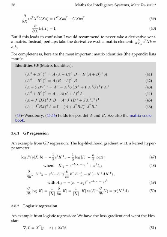
∂
∂X(a>X>CXb) = C>Xab>+ CXba> (39)
∂
∂Xtr(X) = I (40)
But if this leads to confusion I would recommend to never take a derivative w.r.t.a matrix. Instead, perhaps take the derivative w.r.t. a matrix element: ∂
∂Xija>Xb =
aibj .
For completeness, here are the most important matrix identities (the appendix listsmore):
Identities 3.5 (Matrix Identities).
(A-1 +B-1)-1 = A (A+B)-1 B = B (A+B)-1 A (41)
(A-1 −B-1)-1 = A (B −A)-1 B (42)
(A+ UBV )-1 = A-1 −A-1U(B-1 + V A-1U)-1V A-1 (43)
(A-1 +B-1)-1 = A−A(B +A)-1A (44)
(A+ J>BJ)-1J>B = A-1J>(B-1 + JA-1J>)-1 (45)
(A+ J>BJ)-1A = I− (A+ J>BJ)-1J>BJ (46)
(43)=Woodbury; (45,46) holds for pos def A and B. See also the matrix cook-book.
3.6.1 GP regression
An example from GP regression: The log-likelihood gradient w.r.t. a kernel hyper-parameter:
logP (y|X, b) = −1
2y>K -1y − 1
2log |K| − n
2log 2π (47)
where Kij = e−b(xi−xj)2
+ σ2δij (48)∂
∂by>K -1y = y>(−K -1(
∂
∂bK)K -1) = y>(−K -1AK -1) ,
with Aij = −(xi − xj)2 e−b(xi−xj)2
(49)∂
∂blog |K| = 1
|K|∂
∂b|K| = 1
|K||K| tr(K -1 ∂
∂bK) = tr(K -1A) (50)
3.6.2 Logistic regression
An example from logistic regression: We have the loss gradient and want the Hes-sian:
∇βL = X>(p− x) + 2λIβ (51)

Maths for Intelligence Systems, Marc Toussaint 39
where pi = σ(x>iβ) , σ(z) =ez
1 + ez, σ′(z) = σ(z) (1− σ(z)) (52)
∇2β L =
∂
∂β∇βL = X>
∂
∂βp+ 2λ (53)
∂
∂βpi = pi(1− pi) x>i (54)
∂
∂βp = diag([pi(1− pi)]ni=1) X = diag(p (1− p)) X (55)
∇2β L = X>diag(p (1− p)) X + 2λI (56)
(Where is the element-wise product.)
3.7 Check your gradients numerically!
This is your typical work procedure when implementing a Machine Learning orAI’ish or Optimization kind of methods:
• You first mathematically (on paper/LaTeX) formalize the problem domain,including the objective function.
• You derive analytically (on paper) the gradients/Hessian of your objectivefunction.
• You implement the objective function and these analytic gradient equationsin Matlab/Python/C++, using linear algebra packages.
• You test the implemented gradient equations by comparing them to a finitedifference estimate of the gradients!
• Only if that works, you put everything together, interfacing the objective &gradient equations with some optimization algorithm
Algorithm 1 Finite Difference Jacobian Check
Input: x ∈ Rn, function f : Rn → Rn, function df : Rn → Rd×n1: initialize J ∈ Rd×m, and ε = 10−6
2: for i = 1 : n do3: J·i = [f(x+ εei)− f(x− εei)]/2ε // assigns the ith column of J4: end for5: if ||J − df(x)||∞ < 10−4 return true; else false
Here ei is the ith standard basis vector in Rn.
40 Maths for Intelligence Systems, Marc Toussaint
3.8 Examples and Exercises
3.8.1 More derivatives
a) In 3D, note that a×b = skew(a)b = −skew(b)a, where skew(v) is the skew matrixof v. What is the gradient of (a× b)2 w.r.t. a and b?
3.8.2 Minima
a) A core problem in Machine Learning: For β ∈ Rd, y ∈ Rn, X ∈ Rn×d, compute
argminβ||y −Xβ||2 + λ||β||2
b) A core problem in Robotics: For q, q0 ∈ Rn, φ : Rn → Rd, y∗ ∈ Rd non-linearbut smooth, compute
argminq||φ(q)− y∗||2C + ||q − q0||2W
3.8.3 Multivariate Calculus
Given tensors y ∈ Ra×...×z and x ∈ Rα×...×ω where y is a function of x, the Jacobiantensor J = ∂xy is in Ra×...×z×α×...×ω and has coefficients
Ji,j,k,...,l,m,n... =∂
∂xl,m,n,...yi,j,k,...
(All “output” indices come before all “input” indices“.)
Compute the following Jacobian tensors
(i) ∂∂xx, where x is a vector
(ii) ∂∂xx>Ax, where A is a matrix
(iii) ∂∂Ay>Ax, where x and y are vectors (note, we take the derivative w.r.t. A)
(iv) ∂∂AAx
(v) ∂∂xf(x)>Ag(x), where f and g are vector-valued functions

Maths for Intelligence Systems, Marc Toussaint 41
3.8.4 Finite Difference Gradient Checking
The following exercises will require you to code basic functions and derivatives.You can code in your prefereed language (Matlab, NumPy, Julia, whatever).
(i) Implement the following pseudo code for empirical gradient checking in theprogramming language of your choice:
Input: x ∈ Rn, function f : Rn → Rd, function df : Rn → Rd×n
1: initialize J ∈ Rd×n, and ε = 10−6
2: for i = 1 : n do3: J·i = [f(x+ εei)− f(x− εei)]/2ε // assigns the ith column of J4: end for5: if ||J − df(x)||∞ < 10−4 return true; else false
Here ei is the ith standard basis vector in Rn.
(ii) Test this for
• f : x 7→ Ax, df : x 7→ A, where you sample x ∼@randn(n,1)@ (N(0, 1) inMatlab) and A ∼@randn(m,n)@
• f : x 7→ x>x, df : x 7→ 2x>, where x ∼@randn(n,1)@
3.8.5 Backprop in a Neural Net
Consider the function
f : Rh0 → Rh3 , f(x0) = W2σ(W1σ(W0x0))
where Wl ∈ Rhl+1×hl and σ : R → R is a differentiable activation function which isapplied element-wise. We also describe the function as the computation graph:
x0 7→ z1 = W0x0 7→ x1 = σ(z1) 7→ z2 = W1x1 7→ x2 = σ(z2) 7→ f = W2x2
Derive pseudo code to efficiently compute dfdx0
. (Ideally also for deeper networks.)
3.8.6 Backprop in a Neural Net
We consider again the function
f : Rh0 → Rh3 , f(x0) = W2σ(W1σ(W0x0)) ,
where Wl ∈ Rhl+1×hl and σ : R → R is a differentiable activation function which isapplied element-wise. We established last time that
df
dx0=
∂f
∂x2
∂x2
∂z2
∂z2
∂x1
∂x1
∂z1
∂z1
∂x0

42 Maths for Intelligence Systems, Marc Toussaint
with:∂xl∂zl
= diag(xl (1− xl)) ,∂zl+1
∂xl= Wl ,
∂f
∂x2= W2
Note: In the following we still let f be a h3-dimensional vector. For those that areconfused with the resulting tensors, simplify to f being a single scalar output.
(i) Derive also the necessary equations to get the derivative w.r.t. the weight ma-trices Wl, that is the Jacobian tensor
df
dWl
(ii) Write code to implement f(x) and dfdx0
and dfdWl
.
To test this, choose layer sizes (h0, h1, h2, h3) = (2, 10, 10, 2), i.e., 2 input and2 output dimensions, and hidden layers of dimension 10.
For testing, choose random inputs sampled from x ∼@randn(2,1)@
And choose random weight matrices Wl ∼ 1√hl+1
@rand(h[l+1],h[l])@.
Check the implemented Jacobian by comparing to the finite difference ap-proximation.
Debugging Tip: If your first try does not work right away, the typical ap-proach to debug is to “comment out” parts of your function f and df . Forinstance, start with testing f(x) = W0x0; then test f(x) = σ(W0x0); thenf(x) = W1σ(W0x0); then I’m sure all bugs are found.
(iii) Bonus: Try to train the network to become the identity mapping. In thesimplest case, use “stochastic gradient descent”, meaning that you samplean input, compute the gradients wl = d(f(x)−x)2
dWl, and make tiny updates
Wl ←Wl − αwl.
3.8.7 Logistic Regression Gradient & Hessian
Consider the function
L : Rd → R : L(β) = −n∑i=1
[yi log σ(x>iβ) + (1− yi) log[1− σ(x>iβ)]
]+ λβ>β ,
where xi ∈ Rd is the ith row of a matrix X ∈ Rn×d, and y ∈ 0, 1n is a vectorof 0s and 1s only. Here, σ(z) = 1/(e−z + 1) is the sigmoid function, with σ′(z) =σ(z)(1− σ(z)).
Derive the gradient ∂∂βL(β), as well as the Hessian
∇2L(β) =∂2
∂β2L(β) .

Maths for Intelligence Systems, Marc Toussaint 43
4 Optimization
4.1 Downhill algorithms for unconstrained optimization
We discuss here algorithms that have one goal: walk downhill as quickly as possi-ble. These target at efficiently finding local optima—in constrast to global optimiza-tion methods, which try to find the global optimum.
For such downhill walkers, there are two essential things to discuss: the stepsizeand the step direction. When discussing the stepsize we’ll hit on topics like back-tracking line search, the Wolfe conditions and its implications in a basic conver-gence proof. The discussion of the step direction will very much circle around New-ton’s method and thereby also cover topics like quasi-Newton methods (BFGS),Gauss-Newton, covariant and conjugate gradients.
4.1.1 Why you shouldn’t trust the magnitude of the gradient
Consider the following 1D function and naive gradient descent x ← x − α∇f forsome fixed and small α.
large gradient large step?
small gradient small step?
• In plateaus we’d make small steps, at steep slopes (here close to the opti-mum) we make huge steps, very likely overstepping the optimum. In fact,for some α the algorithm might indefinitely loop a non-sensical sequence ofvery slowly walking left on the plateau, then accellerating, eventually over-stepping the optimum, then being thrown back far to the right again becauseof the huge negative gradient on the left.
• Generally, never trust an algorithm that depends on the scaling—or choiceof units—of a function! An optimization algorithm should be invariant onwhether you measure costs in cents or Euros! Naive gradient descent x ←x− α∇f is not!

44 Maths for Intelligence Systems, Marc Toussaint
As a conclusion, the gradient ∇f gives a reasonable descent direction, but its mag-nitude is really arbitrary and no good indication of a good stepsize. Therefore, itoften makes sense to just compute the step direction
δ = − 1
|∇f(x)|∇f(x)
and iterate x← x+ αδ for some appropriate stepsize.
4.1.2 Ensuring monotone and sufficient decrease: Backtracking line search, Wolfeconditions, & convergence
The first idea is simple: If a step would increase the objective value, reduce thestepsize. We typically use multiplicative stepsize adaptations: Reduce α ← %−ααwith %−α ≈ 0.5; and increase α ← %+
αα with %+α ≈ 1.2. A simple monotone gradient
descent algorithm reads as follows (the blue part is explained later). Here, the step
Algorithm 2 Plain gradient descentInput: initial x ∈ Rn, functions f(x) and∇f(x), tolerance θ, parameters (defaults:
%+α = 1.2, %−α = 0.5, δmax =∞, %ls = 0.01)
1: initialize stepsize α = 12: repeat3: δ ← − ∇f(x)
|∇f(x)| // (alternative: δ = −∇f(x))4: while f(x+ αδ) > f(x)+%ls∇f(x)>(αδ) do // line search5: α← %−αα // decrease stepsize6: end while7: x← x+ αδ8: α← min%+
αα, δmax // increase stepsize9: until |αδ| < θ // perhaps for 10 iterations in sequence
vector δ is always normalized and α is adapted on the fly; decreasing when f(x +αδ) is not sufficiently smaller than f(x).
This sufficiently smaller is described by the blue part and is called the (1st) Wolfecondition
f(x+ αδ) > f(x) + %ls∇f(x)>(αδ) .
Figure 3 illustrates this. Note that∇f(x)>(αδ) is a negative value and describes howmuch the objective would decrease if f was linear. But f is of course not linear; wecannot expect that a step would really decrease f that much. Instead we requirethat it decreases by a fraction of this expectation. %ls describes this fraction andis typically chosen very moderate, e.g. %ls ∈ [0.01, 0.1]. So, the Wolfe conditionsrequires that f descreases by the %ls-fraction of what it would decrease if f waslinear. Note that for α → 0 the Wolfe condition will always be fulfilled for smoothfunctions, because f “becomes locally linear”.

Maths for Intelligence Systems, Marc Toussaint 45
Figure 3: The 1st Wolfe condition: f(x)+∇f(x)>(αδ) is the tangent, which describesthe expected decrease of f(x + αδ) if f was linear. We cannot expect this to be thecase; so f(x+ αδ) > f(x) + %ls∇f(x)>(αδ) weakens this condition.
In the exercises you prove that any algorithms that, in each iteration, finds a newpoint that fulfills the Wolfe condition will converge with a convergence rate (1 −2m%ls%
−α
M ) if m > 0 and M > m are lower and upper bounds on the hessian eigenval-ues.
There is a second Wolfe condition,
|∇f(x+ αδ)>δ| ≤ b|∇f(x)>δ| ,
which states that the gradient magnitude should have decreased sufficiently. Wedo not use it much.
4.1.3 The Newton direction
We already discussed the steepest descent direction −G-1∇f(x) if G is a metric tensor.Let’s keep this in mind!
The original Newton method is a method to find the root (that is, zero point) ofa function f(x). In 1D it iterates x ← x − f(x)
f ′(x) , that is, it uses the gradient f ′
to estimate where the function might cross the x-axis. To find an minimum ormaximum of f we want to find the root of its gradient. For x ∈ Rn the Newtonmethod iterates
x← x−∇2f(x)-1∇f(x) .
Note that the Newton step δ = −∇2f(x)-1∇f(x) is the solution to
minδ
[f(x) +∇f(x)>δ +
1
2δ>∇2f(x)δ
].
So the Newton method can also be viewed as 1) compute the 2nd-order Taylorapproximation to f at x, and 2) jump to the optimum of this approximation.
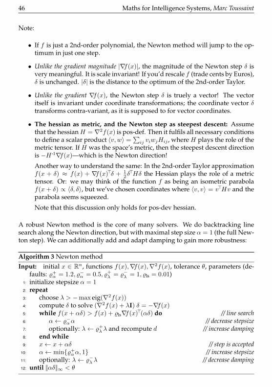
46 Maths for Intelligence Systems, Marc Toussaint
Note:
• If f is just a 2nd-order polynomial, the Newton method will jump to the op-timum in just one step.
• Unlike the gradient magnitude |∇f(x)|, the magnitude of the Newton step δ isvery meaningful. It is scale invariant! If you’d rescale f (trade cents by Euros),δ is unchanged. |δ| is the distance to the optimum of the 2nd-order Taylor.
• Unlike the gradient ∇f(x), the Newton step δ is truely a vector! The vectoritself is invariant under coordinate transformations; the coordinate vector δtransforms contra-variant, as it is supposed to for vector coordinates.
• The hessian as metric, and the Newton step as steepest descent: Assumethat the hessianH = ∇2f(x) is pos-def. Then it fulfils all necessary conditionsto define a scalar product 〈v, w〉 =
∑ij viwjHij , where H plays the role of the
metric tensor. If H was the space’s metric, then the steepest descent directionis −H -1∇f(x)—which is the Newton direction!
Another way to understand the same: In the 2nd-order Taylor approximationf(x + δ) ≈ f(x) + ∇f(x)>δ + 1
2δ>Hδ the Hessian plays the role of a metric
tensor. Or: we may think of the function f as being an isometric parabolaf(x + δ) ∝ 〈δ, δ〉, but we’ve chosen coordinates where 〈v, v〉 = v>Hv and theparabola seems squeezed.
Note that this discussion only holds for pos-dev hessian.
A robust Newton method is the core of many solvers. We do backtracking linesearch along the Newton direction, but with maximal step size α = 1 (the full New-ton step). We can additionally add and adapt damping to gain more robustness:
Algorithm 3 Newton methodInput: initial x ∈ Rn, functions f(x),∇f(x),∇2f(x), tolerance θ, parameters (de-
faults: %+α = 1.2, %−α = 0.5, %+
λ = %−λ = 1, %ls = 0.01)1: initialize stepsize α = 12: repeat3: choose λ > −max eig(∇2f(x))4: compute δ to solve (∇2f(x) + λI) δ = −∇f(x)5: while f(x+ αδ) > f(x) + %ls∇f(x)>(αδ) do // line search6: α← %−αα // decrease stepsize7: optionally: λ← %+
λ λ and recompute d // increase damping8: end while9: x← x+ αδ // step is accepted
10: α← min%+αα, 1 // increase stepsize
11: optionally: λ← %−λ λ // decrease damping12: until ||αδ||∞ < θ
Maths for Intelligence Systems, Marc Toussaint 47
Some notes on the λ:
• The first line chooses λ to ensure that (∇2f(x)+λI) is indeed pos-dev—and aNewton step actually decreases f instead of seeking for a maximum. Clearlythere would be other options: instead of adding to all eigenvalues we couldonly set the negative ones to some λ > 0.
• δ solves the problem
minδ
[∇f(x)>δ +
1
2δ>∇2f(x)δ +
1
2λδ2)
].
So, we added a squared potential λδ2 to the local 2nd-order Taylor approxi-mation. This is like introducing a squared penalty for large steps!
• Trust region method: Let’s consider a different mathematical program overthe step:
minδ∇f(x)>δ +
1
2δ>∇2f(x)δ s.t. δ2 ≤ β
This problem wants to find the minimum of the 2nd-order Taylor (like theNewton step), but constrained to a stepsize no larger than β. This β definesthe trust region: The region in which we trust the 2nd-order Taylor to be areasonable enough approximation.
Let’s solve this as we learned to: Let’s assume the inequality constraint isactive. Then we have
L(δ, λ) = ∇f(x)>δ +1
2δ>∇2f(x)δ + λ(δ2 − β) (57)
∇δL(δ, λ) = ∇f(x)>+ δ>(∇2f(x) + 2λI) (58)
Setting this to zero gives the step δ = −(∇2f(x) + 2λI)-1∇f(x).
Therefore, the λ can be viewed as dual variable of a trust region method.There is no analytic relation between β and λ; we can’t determine λ directlyfrom β. We could use a constrained optimization method, like primal-dualNewton, or Augmented Lagrangian approach to solve for λ and δ. Alter-natively, we can always increase λ when the computed steps are too large,and decrease if they are smaller than β—the Augmented Lagrangian updateequations could be used to do such an update of λ.
• The λδ2 term can be interpreted as penalizing the velocity (stepsizes) of thealgorithm. This is in analogy to a damping, such as “honey damping”, inphysical dynamic systems. The parameter λ is therefore also called damp-ing parameter. Such a damped (or regularized) least-squares methods is alsocalled Levenberg-Marquardt method.
• For λ→∞ the step direction δ becomes aligned with the plain gradient direc-tion−∇f(x). This shows that for λ→∞ the Hessian (and metric deformation
48 Maths for Intelligence Systems, Marc Toussaint
of the space) becomes less important and instead we’ll walk orthogonal to theiso-lines of the function.
• The λ term makes the δ non-scale-invariant! δ is not anymore a proper vector!
4.1.4 Gauss-Newton: a super important special case
A special case that appears really a lot in intelligent systems is the Gauss-Newtoncase: Consider an objective function of the form
f(x) = φ(x)>φ(x) =∑i
φi(x)2 (59)
where we call φ(x) the cost features. This is also called a sum-of-squares problem,here a sum of cost feature squares. We have
∇f(x) = 2∂
∂xφ(x)>φ(x) (60)
∇2f(x) = 2∂
∂xφ(x)>
∂
∂xφ(x) + 2φ(x)>
∂2
∂x2φ(x) (61)
The Gauss-Newton method is the Newton method for f(x) = φ(x)>φ(x) while ap-proximating∇2φ(x) ≈ 0. That is, it computes approximate Newton steps
δ = −(∂
∂xφ(x)>
∂
∂xφ(x) + λI)-1 ∂
∂xφ(x)>φ(x) .
Note:
• The approximate Hessian 2 ∂∂xφ(x)> ∂
∂xφ(x) is always semi-pos-def! There-fore, no problems arise with negative hessian eigenvalues.
• The approximate Hessian only requires the first-order derivatives of the costfeatures. There is no need for computationally expensive hessians of φ.
• The objective f(x) can be interpreted as just the Euclidean norm f(φ) =φ>φ but pulled back into the x-space. More precisely: Consider a mappingφ : Rn → Rm and a general scalar product 〈·, ·〉φ in the output space. Indifferential geometry there is the notion of a pull-back of a metric, that is, wedefine a scalar product 〈·, ·〉x in the input space as
〈x, y〉x = 〈dφ(x), dφ(y)〉φ (62)
where dφ is the differential of φ (a Rm-valued 1-form). Assuming φ-coordinatessuch that the metric tensor of 〈·, ·〉φ is Euclidean, we have
〈x, x〉x = 〈dφ(x), dφ(x)〉φ =∂
∂xφ(x)>
∂
∂xφ(x) (63)
and therefore, the approximate Hessian is the pullback of a Euclidean costfeature metric, and 〈x, x〉x approximates the 2-order polynomial term of f(x),with the non-constant (i.e., Riemannian) pull-back metric 〈·, ·〉x.

Maths for Intelligence Systems, Marc Toussaint 49
4.1.5 Quasi-Newton & BFGS: approximating the hessian from gradient obser-vations
To apply full Newton methods we need to be able to compute f(x),∇f(x), and∇2f(x) for any x. However, sometimes, computing∇2f(x) is not possible, e.g., be-cause we can’t derive an analytic expression for∇2f(x), or it would be to expensiveto compute the hessian exactly, or even to store it in memory—especially in veryhigh-dimensional spaces. In such cases it makes sense to approximate ∇2f(x) or∇2f(x)-1 with a low-rank approximation.
Assume we have computed ∇f(x1) and ∇f(x2) at two different points x1, x2 ∈ Rn.We define
y = ∇f(x2)−∇f(x1) , δ = x2 − x1 .
From this we may wish to find some approximate Hessian matrix H or H -1 thatfulfils
H δ!= y or δ
!= H -1y
The first equation is called secant equation. Here are guesses of H and H -1:
H =yy>
y>δor H -1 =
δδ>
δ>y
Convince yourself that these choices fulfil the respective desired relation above.However, these choices are under-determined. There exist many alternative H orH -1 that would be consistent with the observed change in gradient. However, givenour understanding of the structure of matrices it is clear that these choices are thelowest rank solutions, namely rank 1.
Broyden-Fletcher-Goldfarb-Shanno (BFGS): An optimization algorithm computes∇f(xk) at a series of points x0:K . We incrementally update our guess of H -1 with anupdate equation
H -1 ←(I− yδ>
δ>y
)>H -1(I− yδ>
δ>y
)+δδ>
δ>y,
which is equivalent to (using the Sherman-Morrison formula)
H ← H − Hδδ>H>
δTHδ+yy>
y>δ
Note:
• IfH -1 is initially zero, this update will assignH -1 ← δδ>
δ>y, which is the minimal
rank 1 update we discussed above.
• If H -1 is previously non-zero, the red part “deletes certain dimensions” fromH -1. More precisely, note that
(I− yδ>
δ>y
)y = 0, that is, this construction deletes
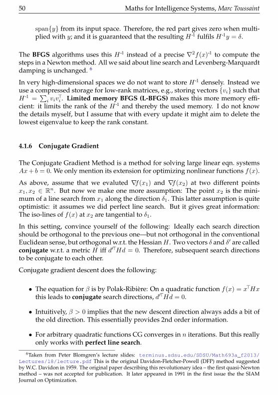
50 Maths for Intelligence Systems, Marc Toussaint
spany from its input space. Therefore, the red part gives zero when multi-plied with y; and it is guaranteed that the resulting H -1 fulfils H -1y = δ.
The BFGS algorithms uses this H -1 instead of a precise ∇2f(x)-1 to compute thesteps in a Newton method. All we said about line search and Levenberg-Marquardtdamping is unchanged. 6
In very high-dimensional spaces we do not want to store H -1 densely. Instead weuse a compressed storage for low-rank matrices, e.g., storing vectors vi such thatH -1 =
∑i viv
>i . Limited memory BFGS (L-BFGS) makes this more memory effi-
cient: it limits the rank of the H -1 and thereby the used memory. I do not knowthe details myself, but I assume that with every update it might aim to delete thelowest eigenvalue to keep the rank constant.
4.1.6 Conjugate Gradient
The Conjugate Gradient Method is a method for solving large linear eqn. systemsAx+ b = 0. We only mention its extension for optimizing nonlinear functions f(x).
As above, assume that we evaluted ∇f(x1) and ∇f(x2) at two different pointsx1, x2 ∈ Rn. But now we make one more assumption: The point x2 is the mini-mum of a line search from x1 along the direction δ1. This latter assumption is quiteoptimistic: it assumes we did perfect line search. But it gives great information:The iso-lines of f(x) at x2 are tangential to δ1.
In this setting, convince yourself of the following: Ideally each search directionshould be orthogonal to the previous one—but not orthogonal in the conventionalEuclidean sense, but orthogonal w.r.t. the HessianH . Two vectors δ and δ′ are calledconjugate w.r.t. a metric H iff d′>Hd = 0. Therefore, subsequent search directionsto be conjugate to each other.
Conjugate gradient descent does the following:
• The equation for β is by Polak-Ribiere: On a quadratic function f(x) = x>Hxthis leads to conjugate search directions, d′>Hd = 0.
• Intuitively, β > 0 implies that the new descent direction always adds a bit ofthe old direction. This essentially provides 2nd order information.
• For arbitrary quadratic functions CG converges in n iterations. But this reallyonly works with perfect line search.
6Taken from Peter Blomgren’s lecture slides: terminus.sdsu.edu/SDSU/Math693a_f2013/Lectures/18/lecture.pdf This is the original Davidon-Fletcher-Powell (DFP) method suggestedby W.C. Davidon in 1959. The original paper describing this revolutionary idea – the first quasi-Newtonmethod – was not accepted for publication. It later appeared in 1991 in the first issue the the SIAMJournal on Optimization.
Maths for Intelligence Systems, Marc Toussaint 51
Algorithm 4 Conjugate gradient descentInput: initial x ∈ Rn, functions f(x),∇f(x), tolerance θOutput: x
1: initialize descent direction d = g = −∇f(x)2: repeat3: α← argminα f(x+ αd) // line search4: x← x+ αd5: g′ ← g, g = −∇f(x) // store and compute grad6: β ← max
g>(g−g′)g′>g′
, 0
7: d← g + βd // conjugate descent direction8: until |∆x| < θ
Algorithm 5 RpropInput: initial x ∈ Rn, function f(x),∇f(x), initial stepsize α, tolerance θOutput: x
1: initialize x = x0, all αi = α, all gi = 02: repeat3: g ← ∇f(x)4: x′ ← x5: for i = 1 : n do6: if gig′i > 0 then // same direction as last time7: αi ← 1.2αi8: xi ← xi − αi sign(gi)9: g′i ← gi
10: else if gig′i < 0 then // change of direction11: αi ← 0.5αi12: xi ← xi − αi sign(gi)13: g′i ← 0 // force last case next time14: else15: xi ← xi − αi sign(gi)16: g′i ← gi17: end if18: optionally: cap αi ∈ [αmin xi, αmax xi]19: end for20: until |x′ − x| < θ for 10 iterations in sequence
4.1.7 Rprop*
Read through Algorithm 5. Notes on this:
• Stepsize adaptation is done in each coordinate separately!
• The algorithm not only ignores |∇f | but also its exact direction! Only the
52 Maths for Intelligence Systems, Marc Toussaint
gradient signs in each coordinate are relevant. Therefore, the step directionsmay differ up to < 90 from −∇f .
• It often works surprisingly efficient and robust.
• If you like, have a look at:
Christian Igel, Marc Toussaint, W. Weishui (2005): Rprop using the natural gradientcompared to Levenberg-Marquardt optimization. In Trends and Applications in Con-structive Approximation. International Series of Numerical Mathematics, volume 151,259-272.
4.2 The general optimization problem – a mathematical program
Definition 4.1. Let x ∈ Rn, f : Rn → R, g : Rn → Rm, h : Rn → Rl. Anoptimization problem, or mathematical program, is
minx
f(x)
s.t. g(x) ≤ 0 , h(x) = 0
We typically at least assume f, g, h to be differentiable or smooth.
Get an intuition about this problem formulation by considering the following ex-amples. Always discuss where is the optimum, and at the optimum, how the ob-jective f pulls at the point, while the constraints g or h push against it.
• A 1D example: x ∈ R, h(x) = sin(x), g(x) = x2/4 − 1, f some non-linearfunction.
• 2D example: f(x, y) = x (intuition: the objective is constantly pulling to theleft), h(x, y) = 0 is some non-linear path in the plane → the optimum is atthe left-most tangent-point of h. Tangent-point means that the tangent of h isvertical. h pushes to the right (always orthogonal to the zero-line of h).
• 2D example: f(x, y) = x, g(x, y) = y2 − x− 1. The zero-line of g is a parabolatowards the right. The objective f pulls into this parabola; the optimum is inthe ’bottom’ of the parabola, at (1, 0).
• 2D example: f(x, y) = x, g(x, y) = x2 + y2 − 1. The zero-line of g is a circle.The objective f pulls to the left; the optimum is at the left tangent-point of thecircle, at (−1, 0).
• Figure 4
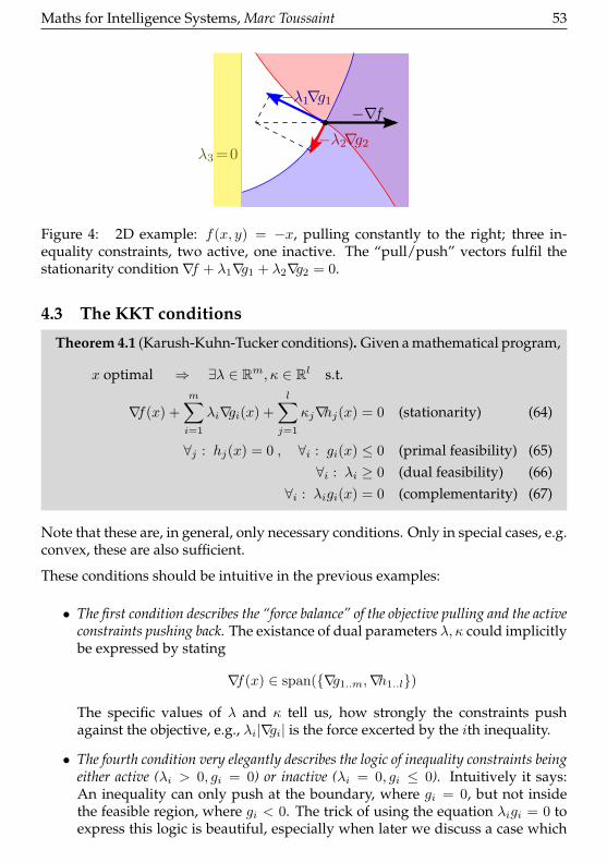
Maths for Intelligence Systems, Marc Toussaint 53
Figure 4: 2D example: f(x, y) = −x, pulling constantly to the right; three in-equality constraints, two active, one inactive. The “pull/push” vectors fulfil thestationarity condition∇f + λ1∇g1 + λ2∇g2 = 0.
4.3 The KKT conditions
Theorem 4.1 (Karush-Kuhn-Tucker conditions). Given a mathematical program,
x optimal ⇒ ∃λ ∈ Rm, κ ∈ Rl s.t.
∇f(x) +
m∑i=1
λi∇gi(x) +
l∑j=1
κj∇hj(x) = 0 (stationarity) (64)
∀j : hj(x) = 0 , ∀i : gi(x) ≤ 0 (primal feasibility) (65)∀i : λi ≥ 0 (dual feasibility) (66)
∀i : λigi(x) = 0 (complementarity) (67)
Note that these are, in general, only necessary conditions. Only in special cases, e.g.convex, these are also sufficient.
These conditions should be intuitive in the previous examples:
• The first condition describes the “force balance” of the objective pulling and the activeconstraints pushing back. The existance of dual parameters λ, κ could implicitlybe expressed by stating
∇f(x) ∈ span(∇g1..m,∇h1..l)
The specific values of λ and κ tell us, how strongly the constraints pushagainst the objective, e.g., λi|∇gi| is the force excerted by the ith inequality.
• The fourth condition very elegantly describes the logic of inequality constraints beingeither active (λi > 0, gi = 0) or inactive (λi = 0, gi ≤ 0). Intuitively it says:An inequality can only push at the boundary, where gi = 0, but not insidethe feasible region, where gi < 0. The trick of using the equation λigi = 0 toexpress this logic is beautiful, especially when later we discuss a case which
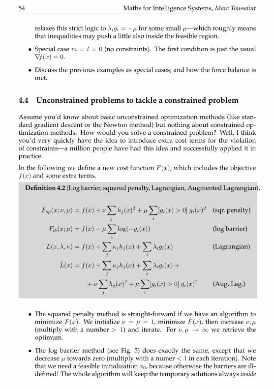
54 Maths for Intelligence Systems, Marc Toussaint
relaxes this strict logic to λigi = −µ for some small µ—which roughly meansthat inequalities may push a little also inside the feasible region.
• Special case m = l = 0 (no constraints). The first condition is just the usual∇f(x) = 0.
• Discuss the previous examples as special cases; and how the force balance ismet.
4.4 Unconstrained problems to tackle a constrained problem
Assume you’d know about basic unconstrained optimization methods (like stan-dard gradient descent or the Newton method) but nothing about constrained op-timization methods. How would you solve a constrained problem? Well, I thinkyou’d very quickly have the idea to introduce extra cost terms for the violationof constraints—a million people have had this idea and successfully applied it inpractice.
In the following we define a new cost function F (x), which includes the objectivef(x) and some extra terms.
Definition 4.2 (Log barrier, squared penalty, Lagrangian, Augmented Lagrangian).
Fsp(x; ν, µ) = f(x) + ν∑j
hj(x)2 + µ∑i
[gi(x) > 0] gi(x)2 (sqr. penalty)
Flb(x;µ) = f(x)− µ∑i
log(−gi(x)) (log barrier)
L(x, λ, κ) = f(x) +∑j
κjhj(x) +∑i
λigi(x) (Lagrangian)
L(x) = f(x) +∑j
κjhj(x) +∑i
λigi(x) +
+ ν∑j
hj(x)2 + µ∑i
[gi(x) > 0] gi(x)2 (Aug. Lag.)
• The squared penalty method is straight-forward if we have an algorithm tominimize F (x). We initialize ν = µ = 1, minimize F (x), then increase ν, µ(multiply with a number > 1) and iterate. For ν, µ → ∞ we retrieve theoptimum.
• The log barrier method (see Fig. 5) does exactly the same, except that wedecrease µ towards zero (multiply with a numer < 1 in each iteration). Notethat we need a feasible initialization x0, because otherwise the barriers are ill-defined! The whole algorithm will keep the temporary solutions always inside
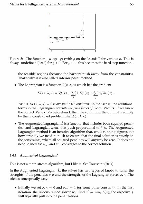
Maths for Intelligence Systems, Marc Toussaint 55
Figure 5: The function −µ log(−g) (with g on the “x-axis”) for various µ. This isalways undefined (“∞”) for g > 0. For µ→ 0 this becomes the hard step function.
the feasible regions (because the barriers push away from the constraints).That’s why it is also called interior point method.
• The Lagrangian is a function L(x, λ, κ) which has the gradient
∇L(x, λ, κ) = ∇f(x) +∑i
λi∇gi(x) +∑j
κj∇hj(x) .
That is, ∇L(x, λ, κ) = 0 is our first KKT condition! In that sense, the additionalterms in the Lagrangian generate the push forces of the constraints. If we knewthe correct λ’s and κ’s beforehand, then we could find the optimal x simplyby the unconstrained problem minx L(x, λ, κ).
• The Augmented Lagrangian L is a function that includes both, squared penal-ties, and Lagrangian terms that push proportional to λ, κ. The AugmentedLagrangian method is an iterative algorithm that, while running, figures outhow strongly we need to push to ensure that the final solution is exactly onthe constraints, where all squared penalties will anyway be zero. It does notneed to increase ν, µ and still converges to the correct solution.
4.4.1 Augmented Lagrangian*
This is not a main-stream algorithm, but I like it. See Toussaint (2014).
In the Augmented Lagrangian L, the solver has two types of knobs to tune: thestrenghts of the penalties ν, µ and the strengths of the Lagrangian forces λ, κ. Thetrick is conceptually easy:
• Initially we set λ, κ = 0 and ν, µ = 1 (or some other constant). In the firstiteration, the unconstrained solver will find x′ = minx L(x); the objective fwill typically pull into the penalizations.

56 Maths for Intelligence Systems, Marc Toussaint
• For the second iteration we then choose parameters λ, κ that try to avoid thatwe will be pulled into penalizations the next time. Let’s update
κj ← κj + 2µhj(x′) , λi ← max(λi + 2µgi(x
′), 0).
Note that 2µhj(x′) is the force (gradient) of the equality penalty at x′; and
max(λi + 2µgi(x′), 0) is the force of the inequality constraint at x′. What this
update does is: it analyzes the forces excerted by the penalties, and translatesthem to forces excerted by the Lagrange terms in the next iteration. It tries totrade the penalizations for the Lagrange terms.
More rigorously, observe that, if f, g, h are linear and the same constraints areactive in two consecutive iterations, then this update will guarantee that allpenalty terms are zero in the second iteration, and therefore the solution ful-fils the first KKT condition (Toussaint, 2014). See also the respective exercise.
4.5 The Lagrangian
4.5.1 How the Lagrangian relates to the KKT conditions
The Lagrangian L(x, κ, λ) = f + κ>h + λ>g has a number of properties that relatesit to the KKT conditions:
(i) Requiring a zero-x-gradient, ∇xL = 0, implies the 1st KKT condition.
(ii) Requiring a zero-κ-gradient, 0 = ∇κL = h, implies primal feasibility (the 2ndKKT condition) w.r.t. the equality constraints.
(iii) Requiring that L is maximized w.r.t. λ ≥ 0 is related to the remaining 2nd and4th KKT conditions:
maxλ≥0
L(x, λ) =
f(x) if g(x) ≤ 0
∞ otherwise(68)
λ = argmaxλ≥0
L(x, λ) ⇒
λi = 0 if gi(x) < 0
0 = ∇λiL(x, λ) = gi(x) otherwise(69)
This implies either (λi = 0 ∧ gi(x) < 0) or gi(x) = 0, which is equivalent tothe complementarity and primal feasibility for inequalities.
These three facts show how tightly the Lagrangian is related to the KKT condi-tions. To simplify the discussion let us assume only inequality constraints fromnow on. Fact (i) tells us that if we minx L(x, λ), we reproduce the 1st KKT condi-tion. Fact (iii) tells us that if we maxλ≥0 L(x, λ), we reproduce the remaining KKTconditions. Therefore, the optimal primal-dual solution (x∗, λ∗) can be character-ized as a saddle point of the Lagrangian. Finding the saddle point can be writtenin two ways:

Maths for Intelligence Systems, Marc Toussaint 57
Definition 4.3 (primal and dual problem).
minx
maxλ≥0
L(x, λ) (primal problem) (70)
maxλ≥0
minx
L(x, λ)︸ ︷︷ ︸l(λ) (dual function)
(dual problem) (71)
Convince yourself, using (68), that the first expression is indeed the original primalproblem
[minx f(x) s.t. g(x) ≤ 0
].
What can we learn from this? The KKT conditions state that, at an optimum, thereexist some λ, κ. This existance statement is not very helpful to actually find them. Incontrast, the Lagrangian tells us directly how the dual parameters can be found: bymaximizing w.r.t. them. This can be exploited in several ways:
4.5.2 Solving mathematical programs analytically, on paper.
Consider the problem
minx∈R2
x2 s.t. x1 + x2 = 1 .
We can find the solution analytically via the Lagrangian:
L(x, κ) = x2 + κ(x1 + x2 − 1)
0 = ∇xL(x, κ) = 2x+ κ11
⇒ x1 = x2 = −κ/2
0 = ∇κL(x, κ) = x1 + x2 − 1 = −κ/2− κ/2− 1 ⇒ κ = −1
⇒x1 = x2 = 1/2
Here we first formulated the Lagrangian. In this context, κ is often called Lagrangemultiplier, but I prefer the term dual variable. Then we find a saddle point of L byrequiring 0 = ∇xL(x, κ), 0 = ∇κL(x, κ). If we want to solve a problem with an in-equality constrained, we do the same calculus for both cases: 1) the constraint is ac-tive (handled like an equality constrained), and 2) the constrained is inactive. Thenwe check if the inactive case solution is feasible, or the active case is dual-feasible(λ ≥ 0). Note that if we have m inequality constraints we have to analytically eval-uate every combination of constraints being active/inactive—which are 2m cases.This already hints at the fact that a real difficulty in solving mathematical programsis to find out which inequality constraints are active or inactive. In fact, if we knewthis a priori, everything would reduce to an equality constrained problem, whichis much easier to solve.

58 Maths for Intelligence Systems, Marc Toussaint
4.5.3 Solving the dual problem, instead of the primal.
In some cases the dual function l(λ) = minx L(x, λ) can analytically be derived. Inthis case it makes very much sense to try solving the dual problem instead of theprimal. First, the dual problem maxλ≥0 l(λ) is guaranteed to be convex even if theprimal is non-convex. (The dual function l(λ) is concave, and the constraint λ ≥ 0convex.) But note that l(λ) is itself defined as the result of a generally non-convexoptimization problem minx L(x, λ). Second, the inequality constraints of the dualproblem are very simple: just λ ≥ 0. Such inequality constraints are called boundconstraints and can be handled with specialized methods, e.g. simple clipping orprojection of steps.
However, in general minx maxy f(x, y) 6= maxy minx f(x, y). For example, in dis-crete domain x, y ∈ 1, 2, let f(1, 1) = 1, f(1, 2) = 3, f(2, 1) = 4, f(2, 2) = 2, andminx f(x, y) = (1, 2) and maxy f(x, y) = (3, 4). Therefore, the dual problem is ingeneral not equivalent to the primal.
The dual function is, for λ ≥ 0, a lower bound
l(λ) = minxL(x, λ) ≤
[minxf(x) s.t. g(x) ≤ 0
].
And consequently
(dual) maxλ≥0
minxL(x, λ) ≤ min
xmaxλ≥0
L(x, λ) (primal)
We say strong duality holds iff
maxλ≥0
minxL(x, λ) = min
xmaxλ≥0
L(x, λ)
If the primal is convex, and there exist an interior point
∃x : ∀i : gi(x) < 0
(which is called Slater condition), then we have strong duality.
4.5.4 Finding the “saddle point” directly with a primal-dual Newton method.
In basic unconstrained optimization an efficient way to find an optimum (mini-mum or maximum) is to find a point where the gradient is zero with a Newtonmethod. At saddle points all gradients are also zero. So, to find a saddle point ofthe Lagrangian we can equally use a Newton method that seeks for roots of the gra-dient. Note that such a Newton method optimizes in the joint primal-dual spaceof (x, κ, λ).
In the case of inequalities, the zero-gradients view is over-simplified: While facts (i)and (ii) characterize a saddle point in terms of zero gradients, fact (iii) makes this

Maths for Intelligence Systems, Marc Toussaint 59
more precise to handle the inequality case. For this reason it is actually easier todescribe the primal-dual Newton method directly in terms of the KKT conditions:We seek a point (x, λ), with λ ≥ 0, that solves the equation system
∇xf(x) + λ>∂xg = 0 (72)diag(λ)g(x) + µ1m = 0 (73)
Note that the first equation is the 1st KKT, and the second is the approximate 4thKKT with log barrier parameter µ (see below). These two equations reflect thesaddle point properties (facts (i) and (iii) above). We define
r(x, λ) = ∇f(x) + λ>∂xgdiag(λ)g(x) + µ1m
(74)
and use the Newton methodxλ
←xλ
− α∇r(x, λ)-1r(x, λ)
to find the root r(x, λ) = 0 (α is the stepsize). We have
∇r(x, λ) =∇2f(x) +
∑i λi∇2gi(x) ∇g(x)>
diag(λ)∇g(x) diag(g(x))
∈ R(n+m)×(n+m) (75)
Note that this method uses the hessians∇2f and∇2g.
The above formulation allows for a duality gap µ. One could choose µ = 0, butoften that is not robust. The beauty is that we can adapt µ on the fly, before eachNewton step, so that we do not need a separate outer loop to adapt µ.
Before computing a Newton step, we compute the current duality gap µ = −∑mi=1 λigi(x).
Then we set µ = 12 µ to half of this. In this way, the Newton step will compute a
direction that aims to half the current duality gap. In practise, this leads to greatconvercence in a single-loop Newton method. (See also Boyd sec 11.7.3.)
The dual feasibility λi ≥ 0 needs to be handled explicitly by the root finder – theline search can simply clip steps to stay within the bound constraints.
Typically, the method is called “interior primal-dual Newton”, in which case alsothe primal feasibility gi ≤ 0 has to be ensured. But I found there tweaks to makethe method also handle infeasible x, including infeasible initializations.
4.5.5 Log Barriers and the Lagrangian
Finally, let’s discuss the log barrier method. In principle it is very simply: For agiven µ, we use an unconstrained solver to find the minimum x∗(µ) of
F (x;µ) = f(x)− µ∑i
log(−gi(x)) .

60 Maths for Intelligence Systems, Marc Toussaint
(This process is also called “centering”.) We then gradually decrease µ to zero,always calling the inner loop to recenter. The generated path of x∗(µ) is calledcentral path.
The method is simple and has very insightful relations to the KKT conditions andthe dual problem. For given µ, the optimality condition is
∇F (x;µ) = 0 ⇒ ∇f(x)−∑i
µ
gi(x)∇gi(x) = 0 (76)
⇔ ∇f(x) +∑i
λi∇gi(x) = 0 , λigi(x) = −µ (77)
where we defined(!) λi = −µ/gi(x), which guarantees λi ≥ 0 as long as we are inthe interior (gi ≤ 0).
So,∇F (x;µ) = 0 is equivalent to the modified (=approximate) KKT conditions, wherethe complemenetarity is relaxed: inequalities may push also inside the feasible re-gion. For µ → 0 we converge to the exact KKT conditions with strict complemen-tarity.
So µ has the interpretation of a relaxation of complementarity. We can derive an-other interpretation of µ in terms of suboptimality or the duality gap:
Let x∗(µ) = minx F (x;µ) be the central path. At each x∗ we may define, as above,λi = −µ/gi(x∗). We note that λ ≥ 0 (dual feasible), as well that x∗(µ) minimizesthe Lagrangian L(x, λ) w.r.t. x! This is because,
0 = ∇F (x, µ) = ∇f(x) +
m∑i=1
λi∇gi(x) = ∇L(x, λ) . (78)
Therefore, x∗ is actually the solution to minx L(x, λ), which defines the dual func-tion. We have
l(λ) = minxL(x, λ) = f(x∗) +
m∑i=1
λigi(x∗) = f(x∗)−mµ . (79)
(m is simply the count of inequalities.) That is, mµ is the duality gap between the(suboptimal) f(x∗) and l(λ). Further, given that the dual function is a lower bound,l(λ) ≤ p∗, where p∗ = minx f(x) s.t. g(x) ≤ 0 is the optimal primal value, wehave
f(x∗)− p∗ ≤ mµ .This gives the interpretation of µ as an upper bound on the suboptimality of f(x∗).
4.6 Convex Problems
We do not put much emphasis on discussing convex problems in this lecture. Thealgorithms we discussed so far equally apply on general non-linear programs as
Maths for Intelligence Systems, Marc Toussaint 61
well as on convex problems—of course, only on convex problems we have conver-gence guarantees, as we can see from the convergence rate analysis of Wolfe stepsbased on the assumption of positive upper and lower bounds on the Hessian’seigenvalues.
Nevertheless, we at least define standard LPs, QPs, etc. Perhaps the most interest-ing part is the discussion of the Simplex algorithm—not because the algorithms isnice or particularly efficient, but rather because one gains a lot of insights in whatactually makes (inequality) constrained problems hard.
4.6.1 Convex sets, functions, problems
Definition 4.4 (Convex set, convex function). A set X ⊆ V (a subset of somevector space V ) is convex iff
∀x, y ∈ X, a ∈ [0, 1] : ax+ (1−a)y ∈ X (80)
A function is defined
convex ⇐⇒ ∀x, y ∈ Rn, a ∈ [0, 1] : f(ax+ (1−a)y) ≤ a f(x) + (1−a) f(y) (81)
quasiconvex ⇐⇒ ∀x, y ∈ Rn, a ∈ [0, 1] : f(ax+ (1−a)y) ≤ maxf(x), f(y) (82)
Note: quasiconvex ⇐⇒ for any α ∈ R the sublevel set x|f(x) ≤ α is convex.Further, I call a function unimodal if it has only one local minimum, which is theglobal minimum.
Definition 4.5 (Convex program).
Variant 1: A mathematical program minx f(x) s.t. g(x) ≤ 0, h(x) = 0 isconvex if f is convex and the feasible set is convex.
Variant 2: A mathematical program minx f(x) s.t. g(x) ≤ 0, h(x) = 0 isconvex if f and every gi are convex and h is linear.
Variant 2 is the stronger and usual definition. Concerning variant 1, if the feasibleset is convex the zero-level sets of all g’s need to be convex and the zero-level sets ofh’s needs to be linear. Above these zero levels the g’s and h’s could in principle beabribtrarily non-linear, but these non-linearities are irrelevant for the mathematicalprogram itself. We could replace such g’s and h’s by convex and linear functionsand get the same problem.
4.6.2 Linear and quadratic programs
Definition 4.6 (Linear program (LP), Quadratic program (QP)). Special case

62 Maths for Intelligence Systems, Marc Toussaint
mathematical programs are
Linear Program (LP): minx
c>x s.t. Gx ≤ h, Ax = b (83)
LP in standard form: minx
c>x s.t. x ≥ 0, Ax = b (84)
Quadratic Program (QP): minx
1
2x>Qx+ c>x s.t. Gx ≤ h, Ax = b ,Qpos-def
(85)
Rarely, also a Quadratically Constrained QP (QCQP) is considered.
An important example for LP are relaxations of integer linear programs,
minxc>x s.t. Ax = b, xi ∈ 0, 1 ,
which includes Travelling Salesman, MaxSAT or MAP inference problems. Relax-ing such a problem means to instead solve the continuous LP
minxc>x s.t. Ax = b, xi ∈ [0, 1] .
If one is lucky and the continuous LP problem converges to a fully integer solution,where all xi ∈ 0, 1, this is also the solution to the integer problem. Typically, thesolution of the continuous LP will be partially integer (some values converge to theextreme xi ∈ 0, 1, while others are inbetween xi ∈ (0, 1)). This continuous valuedsolution gives a lower bound on the integer problem, and provides very efficientheuristics for backtracking or branch-and-bound search for a fully integer solution.
The standard example for a QP are Support Vector Machines. The primal problemis
minβ,ξ||β||2 + C
n∑i=1
ξi s.t. yi(x>iβ) ≥ 1− ξi , ξi ≥ 0
the dual
l(α, µ) = minβ,ξ
L(β, ξ, α, µ) = − 14
n∑i=1
n∑i′=1
αiαi′yiyi′ x>i xi′ +
n∑i=1
αi
maxα,µ
l(α, µ) s.t. 0 ≤ αi ≤ C
(See ML lecture 5:13 for a derivation.)

Maths for Intelligence Systems, Marc Toussaint 63
y
x
A
B
4.6.3 The Simplex Algorithm
Consider an LP. We make the following observations:
• First, in LPs the equality constraints could be resolved simply by introducingnew coordinates along the zero-hyperplane of h. Therefore, for the conceptualdiscussion we neglect equality constraints.
• The objective constantly pulls in the direction −c = −∇f(x).
• If the solution is bounded there need to be some inequality constraints thatkeep the solution from travelling to∞ in the −c direction.
• It follows: The solution will always be located at a vertex, that is, an inter-section point of several zero-hyperplanes of inequality constraints.
• In fact, we should think of the feasible region as a polytope that is defined byall the zero-hyperplanes of the inequalities. The inside the polytope is the fea-sible region. The polytope has edges (intersections of two contraint planes),faces, etc. A solution will always be located at a vertex of the polytope; moreprecisely, there could be a whole set of optimal points (on a face orthogonalto c), but at least one vertex is also optimal.
• An idea for finding the solution is to walk on the edges of the polytopeuntil an optimal vertex is found. This is the simplex algorithm of GeorgDantzig, 1947. In practise this procedure is done by “pivoting on the sim-plex tableaux”—but we fully skip such details here.
• The simplex algorithm is often efficient, but in worst case it is exponentialin both, n and m! This is hard to make intuitive, because the effects of highdimensions are not intuitive. But roughly, consider that in high dimensionsthere is a combinatorial number of ways of how constraints may intersect andform edges and vertices.

64 Maths for Intelligence Systems, Marc Toussaint
Here is a view that much more relates to our discussion of the log barrier method:Sitting on an edge/face/vertex is equivalent to temporarily deciding which con-straints are active. If we knew which constraints are eventually active, the problemwould be solved: all inequalities become equalities or void. (And linear equalitiescan directly be solved for.) So, jumping along vertices of the polytope is equiva-lent to sequentially making decisions on which constraints might be active. Notethough that there are 2m configurations of active/non-active constraints. The sim-plex algorithm therefore walks through this combinatorial space.
Interior point methods do exactly the opposite: Recall that the 4th KKT conditionis λigi(x) = 0. The log barrier method (for instance) instead relaxes this hard logic ofactiv/non-active constraints and finds in each iteration a solution to the relaxed 4thKKT condition λigi(x) = −µ, which intuitively means that every constraint may be“somewhat active”. In fact, every constraint contributes somewhat to the station-arity condition via the log barrier’s gradients. Thereby interior point methods
• post-pone the hard decisions about active/non-active constraints
• approach the optimal vertex from the inside of the polytope; avoiding thepolytope surface (and its hard decisions)
• thereby avoids the need to search through a combinatorial space of constraintactivities and instead continuously converges to a decision
• has polynomial worst-case guaranteed
Historically, penalty and barrier methods methods were standard before the Sim-plex Algorithm. When SA was discovered in the 50ies, it was quickly consideredgreat. But then, later in the 70-80ies, a lot more theory was developed for interiorpoint methods, which now again have become somewhat more popular than thesimplex algorithm.
4.6.4 Sequential Quadratic Programming
Just for reference, SQP is another standard approach to solving non-linear math-ematical programs. In each iteration we compute all coefficients of the 2nd or-der Taylor f(x + δ) ≈ f(x) + ∇f(x)>δ + 1
2δ>Hδ and 1st-order Taylor g(x + δ) ≈
g(x) +∇g(x)>δ and then solve the QP
minδ
f(x) +∇f(x)>δ +1
2δ>∇2f(x)δ s.t. g(x) +∇g(x)>δ ≤ 0
The optimal δ∗ of this problem should be seen analogous to the optimal Newtonstep: If f were a 2nd-order polynomial and g linear, then δ∗ would jump directlyto the optimum. However, as this is generally not the case, δ∗ only gives us avery good direction for line search. In SQP, we need to backtrack until we found afeasible point and f decreases sufficiently.
Maths for Intelligence Systems, Marc Toussaint 65
Solving each QP in the sub-routine requires a constrained solver, which itself mighthave two nested loops (e.g. using log-barrier or AugLag). In that case, SQP hasthree nested loops.
4.7 Blackbox & Global Optimization: It’s all about learning
Even if f, g, h are smooth, the solver might not have access to analytic equations orefficient numeric methods to evaluate the gradients or hessians of these. Thereforewe distinguish (here neglecting the constraint functions g and h):
Definition 4.7.
• Blackbox optimization: Only f(x) can be evaluated.
• 1st-order/gradient optimization: Only f(x) and∇f(x) can be evaluated.
• Quasi-Newton optimization: Only f(x) and∇f(x) can be evaluated, but thesolver does tricks to estimate∇2f(x). (So this is a special case of 1st-orderoptimization.)
• Gauss-Newton type optimization: f is of the special form f(x) = φ(x)>φ(x)and ∂
∂xφ(x) can be evaluated.
• 2nd order optimization: f(x),∇f(x) and ∇2f(x) can be evaluated.
In this lecture I very briefly want to add comments on global blackbox optimiza-tion. Global means that we now, for the first time, really aim to find the globaloptimum (within some pre-specified bounded range). In essence, to address such aproblem we need to explicitly know what we know about f 7, and an obvious wayto do this is to use Bayesian learning.
4.7.1 A sequential decision problem formulation
From now on, let’s neglect constraints and focus on the mathematical program
minxf(x)
for a blackbox function f . The optimization process can be viewed as a Markov De-cision Process that describes the interaction of the solver (agent) with the function(environment):
• At step t, Dt = (xi, yi)t-1i=1 is the data that the solver has collected fromprevious samples. This Dt is the state of the MDP.
7Cf. the KWIK (knows what it knows) framework.

66 Maths for Intelligence Systems, Marc Toussaint
• At step t, the solver may choose a new decision xt about where to samplenext.
• Given state Dt and decision xt, the next state is Dt+1 = D ∪ (xt, f(xt)),which is a deterministic transition given the function f .
• A solver policy is a mapping π : Dt 7→ xt that maps any state (of knowledge)to a new decision.
• We may define an optimal solver policy as
π∗ = argminπ〈yT 〉 = argmin
π
∫f
P (f) P (DT |π, f) yT
where P (DT |π, f) is deterministic, and P (f) is a prior over functions.
This objective function cares only about the last value yT sampled by thesolver for a fixed time horizon (budget) T . Alternatively, we may chooseobjectives
∑Tt=1 yt or
∑Tt=1 γ
tyt for some discounting γ ∈ [0, 1]
The above defined what is an optimal solver! Something we haven’t touched at allbefore. The transition dynamics of this MDP is deterministic, given f . However,from the perspective of the solver, we do not know f apriori. But we can alwayscompute a posterior belief P (f |Dt) = P (Dt|f) P (f)/P (Dt). This posterior beliefdefines a belief MDP with stochastic transitions
P (Dt+1) =
∫Dt
∫f
∫xt
[Dt+1 = D ∪ (xt, f(xt))] π(xt|Dt) P (f |Dt) P (Dt) .
The belief MDP’s state space is P (Dt) (or equivalently, P (f |Dt), the current beliefover f ). This belief MDP is something that the solver can, in principle, forwardsimulate—it has all information about it. One can prove that, if the solver couldsolve its own belief MDP (find an optimal policy for its belief MDP), then this policyis the optimal solver policy for the original problem given a prior distribution P (f)!So, in principle we not only defined what is an optimal solver policy, but can alsoprovide an algorithm to compute it (Dynamic programming in the belief MDP)!However, this is so expensive to compute that heuristics need to be used in practise.
One aspect we should learn from this discussion: The solver’s optimal decisionis based on its current belief P (f |Dt) over the function. This belief is the Bayesianrepresentation of everything one could possibly have learned about f from the dataDt collected so far. Bayesian Global Optimization methods compute P (f |Dt) inevery step and, based on this, use a heuristic to choose the next decision.
4.7.2 Acquisition Functions for Bayesian Global Optimization*
In pratice one typically uses a Gaussian Process representation of P (f |Dt). Thismeans that in every iteration we have an estimate f(x) of the function mean and

Maths for Intelligence Systems, Marc Toussaint 67
a variance estimate σ(x)2 that describes our uncertainty about the mean estimate.Based on this we may define the following acquisition functions
Definition 4.8. Probability of Improvement (MPI)
αt(x) =∫ y∗−∞N(y|f(x), σ(x)) dy
Expected Improvement (EI)
αt(x) =∫ y∗−∞N(y|f(x), σ(x)) (y∗ − y) dy
Upper Confidence Bound (UCB)
αt(x) = −f(x) + βtσ(x)
Predictive Entropy Search Hernandez-Lobato et al. (2014)
αt(x) = H[p(x∗|Dt)]− Ep(y|Dt;x)H[p(x∗|Dt ∪ (x, y))] (86)= I(x∗, y|Dt) = H[p(y|Dt, x)]− Ep(x∗|Dt)H[p(y|Dt, x, x
∗)] (87)
The last one is special; we’ll discuss it below.
These acquisition functions are heuristics that define how valuable it is to acquiredata from the site x. The solver then makes the decision
xt = argmaxx
αt(x) .
MPI is hardly being used in practise anymore. EI is classical, originating way backin the 50ies or earlier; Jones et al. (1998) gives an overview. UCB received a lot of at-tention recently due to the underlying bandit theory and bounded regret theoremsdue to the submodularity. But I think that in practise EI and UCB perform aboutequally. As UCB is somewhat easier to implement and intuitive.
In all cases, note that the solver policy xt = argmaxx αt(x) requires to internallysolve another non-linear optimization problem. However, αt is an analytic func-tion for which we can compute gradients and hessians which ensures every effi-cient local convergence. But again, xt = argmaxx αt(x) needs to be solved glob-ally—otherwise the solver will also not solve the original problem properly andglobally. As a consequence, the optimization of the acquisition function needs tobe restarted from many many potential start points close to potential local minima;typically from grid(!) points over the full domain range. The number of grid pointsis exponential in the problem dimension n. Therefore, this inner loop can be veryexpensive.
And a subjective note: This all sounds great, but be aware that Gaussian Processeswith standard squared-exponential kernels do not generalize much in high dimen-sions: one roughly needs exponentially many data points to fully cover the domain
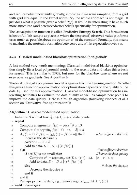
68 Maths for Intelligence Systems, Marc Toussaint
and reduce belief uncertainty globally, almost as if we were sampling from a gridwith grid size equal to the kernel width. So, the whole approach is not magic. Itjust does what is possible given a belief P (f). It would be interesting to have muchmore structured (and heteroscedastic) beliefs specifically for optimization.
The last acquisition function is called Predictive Entropy Search. This formulationis beautiful: We sample at places x where the (expected) observed value y informsus as much as possible about the optimum x∗ of the function! Formally, this meansto maximize the mutual information between y and x∗, in expectation over y|x.
4.7.3 Classical model-based blackbox optimization (non-global)*
A last method very worth mentioning: Classical model-based blackbox optimiza-tion simply fits a local polynomial model to the recent data and takes this a basisfor search. This is similar to BFGS, but now for the blackbox case where we noteven observe gradients. See Algorithm 6.
The local fitting of a polynomial model is again a Machine Learning method. Whetherthis gives a function approximation for optimization depends on the quality of thedata Dt used for this approximation. Classical model-based optimization has in-teresting heuristics to evaluate the data quality as well as sample new points toimprove the data quality. Here is a rough algorithm (following Nodecal et al.’ssection on “Derivative-free optimization”):
Algorithm 6 Classical model-based optimization
1: Initialize D with at least 12 (n+ 1)(n+ 2) data points
2: repeat3: Compute a regression f(x) = φ2(x)>β on D4: Compute δ = argminδ f(x+ δ) s.t. |δ| < α
5: if f(x+ δ) < f(x)− %ls[f(x)− f(x+ δ)] then // test sufficient decrease6: Increase the stepsize α7: Accept x← x+ δ8: Add to data, D ← D ∪ (x, f(x))9: else // no sufficient decrease
10: if det(D) is too small then // blame the data quality11: Compute x+ = argmaxx′ det(D ∪ x′) s.t. |x− x′| < α12: Add to data, D ← D ∪ (x+, f(x+))13: else // blame the stepsize14: Decrease the stepsize α15: end if16: end if17: Perhaps prune the data, e.g., remove argmaxx∈∆ det(D \ x)18: until x converges
Maths for Intelligence Systems, Marc Toussaint 69
Some notes:
• Line 4 implement an explicit trust region approach, which hard bound α onthe step size.
• Line 5 is like the Wolfe condition. But here, the expected decrease is [f(x) −f(x+ δ)] instead of −αδ∇f(x).
• If there is no sufficient decrease we may blame it on two reasons: bad data ora too large stepsize.
• Line 10 uses the data determinant as a measure of quality! This is meant inthe sense of linear regression on polynomial features. Note that, with datamatrix X ∈ Rn×dim(β), βls = (X>X)-1X>y is the optimal regression. Thedeterminant det(X>X) or det(X) = det(D) is a measure for well the datasupports the regression. If the determinant is zero, the regression problem isill-defined. The larger the determinant, the lower the variance of the regres-sion estimator.
• Line 11 is an explicit exploration approach: We add a data point solely for thepurpose of increasing the data determinant (increasing the data spread). In-teresting. Nocedal describes in more detail a geometry-improving procedureto update D.
4.7.4 Evolutionary Algorithms*
There are interesting and theoretically well-grounded evolutionary algorithms foroptimization, such as Estimation-of-Distribution Algorithms (EDAs). But gener-ally, don’t use them as first choice.
4.8 Examples and Exercises
4.8.1 Convergence proof
a) Given a function f : Rn → R with fmin = minx f(x). Assume that its Hessian—that is, the eigenvalues of ∇2f—are lower bounded by m > 0 and upper boundedby M > m, with m,M ∈ R. Prove that for any x ∈ Rn it holds
f(x)− 1
2m|∇f(x)|2 ≤ fmin ≤ f(x)− 1
2M|∇f(x)|2 .
Tip: Start with bounding the 2nd-order Taylor expansion. Then consider the min-ima of these bounds. Note, it also follows:
|∇f(x)|2 ≥ 2m(f(x)− fmin) .
70 Maths for Intelligence Systems, Marc Toussaint
b) Consider backtracking line search with Wolfe parameter %ls ≤ 12 , and step de-
crease factor %−α . First prove that line search terminates the latest when %−αM ≤ α ≤
1M , and then it found a new point y for which
f(y) ≤ f(x)− %ls%−α
M|∇f(x)|2 .
From this, using the result from a), prove the convergence equation
f(y)− fmin ≤[1− 2m%ls%
−α
M
](f(x)− fmin) .
4.8.2 Backtracking Line Search
Consider the functions
fsq(x) = x>Cx , (88)
fhole(x) = 1− exp(−x>Cx) . (89)
with diagonal matrix C and entries C(i, i) = ci−1n−1 , where n is the dimensionality of
x. We choose a conditioning8 c = 10. To plot the function for n = 2, you can usegnuplot calling
set isosamples 50,50set contourf(x,y) = x*x+10*y*y#f(x,y) = 1 - exp(-x*x-10*y*y)splot [-1:1][-1:1] f(x,y)
a) Implement gradient descent with backtracking, as described on page 42 (Algo-rithm 2 Plain gradient descent). Test the algorithm on fsq(x) and fhole(x) with startpoint x0 = (1, 1). To judge the performance, create the following plots:
– The function value over the number of function evaluations.– For n = 2, the function surface including algorithm’s search trajectory. If using gnuplot,
store every evaluated point x and function value f(x) in a line (with n + 1 entries) in afile ’path.dat’, and plot using
unset contoursplot [-3:3][-3:3] f(x,y), ’path.dat’ with lines
b) Play around with parameters. How does the performance change for higherdimensions, e.g., n = 100? How does the performance change with ρls (the Wolfestop criterion)? How does the alternative in step 3 work?
8The word “conditioning” generally denotes the ratio of the largest and smallest Eigenvalue of theHessian.
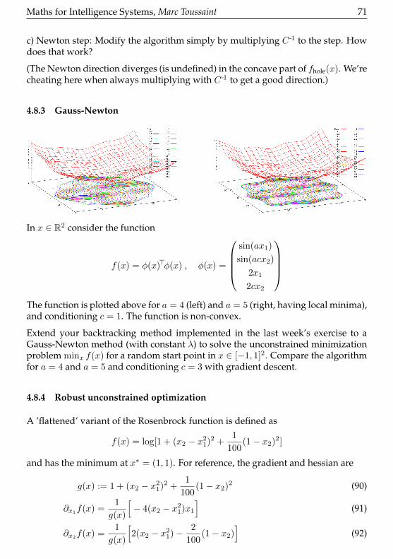
Maths for Intelligence Systems, Marc Toussaint 71
c) Newton step: Modify the algorithm simply by multiplying C -1 to the step. Howdoes that work?
(The Newton direction diverges (is undefined) in the concave part of fhole(x). We’recheating here when always multiplying with C -1 to get a good direction.)
4.8.3 Gauss-Newton
In x ∈ R2 consider the function
f(x) = φ(x)>φ(x) , φ(x) =
sin(ax1)
sin(acx2)
2x1
2cx2
The function is plotted above for a = 4 (left) and a = 5 (right, having local minima),and conditioning c = 1. The function is non-convex.
Extend your backtracking method implemented in the last week’s exercise to aGauss-Newton method (with constant λ) to solve the unconstrained minimizationproblem minx f(x) for a random start point in x ∈ [−1, 1]2. Compare the algorithmfor a = 4 and a = 5 and conditioning c = 3 with gradient descent.
4.8.4 Robust unconstrained optimization
A ’flattened’ variant of the Rosenbrock function is defined as
f(x) = log[1 + (x2 − x21)2 +
1
100(1− x2)2]
and has the minimum at x∗ = (1, 1). For reference, the gradient and hessian are
g(x) := 1 + (x2 − x21)2 +
1
100(1− x2)2 (90)
∂x1f(x) =
1
g(x)
[− 4(x2 − x2
1)x1
](91)
∂x2f(x) =
1
g(x)
[2(x2 − x2
1)− 2
100(1− x2)
](92)

72 Maths for Intelligence Systems, Marc Toussaint
∂2x1f(x) = −
[∂x1
f(x)]2
+1
g(x)
[8x2
1 − 4(x2 − x21)]
(93)
∂2x2f(x) = −
[∂x2
f(x)]2
+1
g(x)
[2 +
2
100
](94)
∂x1∂x2
f(x) = −[∂x1
f(x)][∂x2
f(x)]
+1
g(x)
[− 4x1
](95)
a) Use gnuplot to display the function copy-and-pasting the following lines:
set isosamples 50,50set contourf(x,y) = log(1+(y-(x**2))**2 + .01*(1-x)**2 ) - 0.01splot [-3:3][-3:4] f(x,y)
(The ’-0.01’ ensures that you can see the contour at the optimum.) List and dis-cuss at least three properties of the function (at different locations) that may raiseproblems to naive optimizers.
b) Use x = (−3, 3) as starting point for an optimization algorithm. Try to code anoptimization method that uses all ideas mentioned in the lecture. Try to tune itto be efficient on this problem (without cheating, e.g. by choosing a perfect initialstepsize.)
4.8.5 Lagrangian Method of Multipliers
In a previous exercise we defined the “hole function” f chole(x), assume condition-ing c = 10 and use the Lagrangian Method of Multipliers to solve on paper thefollowing constrained optimization problem in 2D.
minxf chole(x) s.t. h(x) = 0 (96)
h(x) = v>x− 1 (97)
Near the very end, you won’t be able to proceed until you have special values forv. Go as far as you can without the need for these values.
4.8.6 Lagrangian and dual function
(Taken roughly from ‘Convex Optimization’, Ex. 5.1)
A simple example. Consider the optimization problem
minx
x2 + 1 s.t. (x− 2)(x− 4) ≤ 0
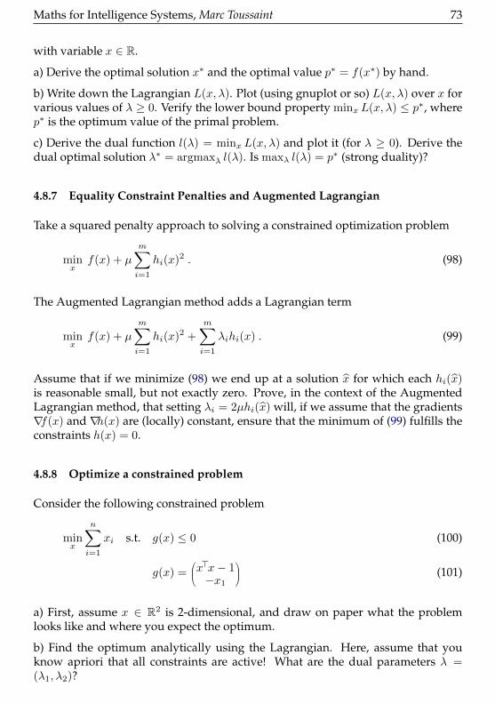
Maths for Intelligence Systems, Marc Toussaint 73
with variable x ∈ R.
a) Derive the optimal solution x∗ and the optimal value p∗ = f(x∗) by hand.
b) Write down the Lagrangian L(x, λ). Plot (using gnuplot or so) L(x, λ) over x forvarious values of λ ≥ 0. Verify the lower bound property minx L(x, λ) ≤ p∗, wherep∗ is the optimum value of the primal problem.
c) Derive the dual function l(λ) = minx L(x, λ) and plot it (for λ ≥ 0). Derive thedual optimal solution λ∗ = argmaxλ l(λ). Is maxλ l(λ) = p∗ (strong duality)?
4.8.7 Equality Constraint Penalties and Augmented Lagrangian
Take a squared penalty approach to solving a constrained optimization problem
minx
f(x) + µ
m∑i=1
hi(x)2 . (98)
The Augmented Lagrangian method adds a Lagrangian term
minx
f(x) + µ
m∑i=1
hi(x)2 +
m∑i=1
λihi(x) . (99)
Assume that if we minimize (98) we end up at a solution x for which each hi(x)is reasonable small, but not exactly zero. Prove, in the context of the AugmentedLagrangian method, that setting λi = 2µhi(x) will, if we assume that the gradients∇f(x) and ∇h(x) are (locally) constant, ensure that the minimum of (99) fulfills theconstraints h(x) = 0.
4.8.8 Optimize a constrained problem
Consider the following constrained problem
minx
n∑i=1
xi s.t. g(x) ≤ 0 (100)
g(x) =x>x− 1−x1
(101)
a) First, assume x ∈ R2 is 2-dimensional, and draw on paper what the problemlooks like and where you expect the optimum.
b) Find the optimum analytically using the Lagrangian. Here, assume that youknow apriori that all constraints are active! What are the dual parameters λ =(λ1, λ2)?
74 Maths for Intelligence Systems, Marc Toussaint
Note: Assuming that you know a priori which constraints are active is a huge as-sumption! In real problems, this is the actual hard (and combinatorial) problem.More on this later in the lecture.
c) Implement a simple the Log Barrier Method. Tips:
– Initialize x = ( 12, 12) and µ = 1
– First code an inner loop:– In each iteration, first compute the gradient of the log-barrier function. Recall that
F (x;µ) = f(x)− µ∑i
log(−gi(x)) (102)
∇F (x;µ) = ∇f − µ∑i
(1/gi(x))∇gi(x) (103)
– Then perform a backtracking line search along −∇F (x, µ). In particular, backtrackif a step goes beyond the barrier (where g(x) 6≤ 0 and F (x, µ) =∞).
– Iterate until convergence; let’s call the result x∗(µ). Further, compute λ∗(m) =−(µ/g1(x), µ/g2(x)) at convergence.
– Decrease µ ← µ/2, recompute x∗(µ) (with the previous x∗ as initialization) and iteratethis.
Does x∗ and λ∗ converge to the expected solution?
Note: The path x∗(µ) = argminx F (x;µ) (the optimum in dependence of µ) is calledcentral path.
4.8.9 Network flow problem
Comment: Solving problems in the real world involves 2 parts:
1) formulating the problem as an optimization problem (→ human)
2) the actual optimization problem (→ algorithm)
The first part is perhaps more interesting – that’s the science part. But under-standing the algorithms helps to better formalize problems. This and the followingexercises are from Boyd & Vandenberghe’s book http://www.stanford.edu/
˜boyd/cvxbook/bv_cvxbook.pdf. They are only about the first part.
Solve Exercise 4.12 (pdf page 207) from Boyd & Vandenberghe, Convex Optimization.
4.8.10 Minimum fuel optimal control
Solve Exercise 4.16 (pdf page 208) from Boyd & Vandenberghe, Convex Optimization.
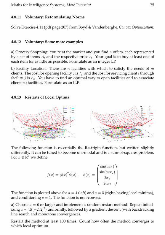
Maths for Intelligence Systems, Marc Toussaint 75
4.8.11 Voluntary: Reformulating Norms
Solve Exercise 4.11 (pdf page 207) from Boyd & Vandenberghe, Convex Optimization.
4.8.12 Voluntary: Some more examples
a) Grocery Shopping: You’re at the market and you find n offers, each representedby a set of items Ai and the respective price ci. Your goal is to buy at least one ofeach item for as little as possible. Formulate as an integer LP.
b) Facility Location: There are n facilities with which to satisfy the needs of mclients. The cost for opening facility j is fj , and the cost for servicing client i throughfacility j is cij . You have to find an optimal way to open facilities and to associateclients to facilities. Formulate as an ILP.
4.8.13 Restarts of Local Optima
The following function is essentially the Rastrigin function, but written slightlydifferently. It can be tuned to become uni-modal and is a sum-of-squares problem.For x ∈ R2 we define
f(x) = φ(x)>φ(x) , φ(x) =
sin(ax1)
sin(acx2)
2x1
2cx2
The function is plotted above for a = 4 (left) and a = 5 (right, having local minima),and conditioning c = 1. The function is non-convex.
a) Choose a = 6 or larger and implement a random restart method: Repeat initial-izing x ∼ U([−2, 2]2) uniformlly, followed by a gradient descent (with backtrackingline search and monotone convergence).
Restart the method at least 100 times. Count how often the method converges towhich local optimum.

76 Maths for Intelligence Systems, Marc Toussaint
4.8.14 UCB Bayesian Optimization
Find an implementation of Gaussian Processes for your language of choice (e.g.python: scikit-learn, or Sheffield/Gpy; octave/matlab: gpml). and implementUCB. Test your implementation with different hyperparameters (Find the best com-bination of kernel and its parameters in the GP) on the 2D function defined above.
4.8.15 No Free Lunch Theorems
Broadly speaking, the No Free Lunch Theorems state that all algorithms perform“in average” exactly the same, if no restrictions or assumptions are made w.r.t. theproblem. Algorithms outperform each other only w.r.t. specific classes of problems.
a) Read the publication “No Free Lunch Theorems for Optimization” by Wolpertand Macready and get a better feel for what the statements are about.
b) You are given an optimization problem where the search space is a discrete setX of integers 1, . . . , 100, and the cost space Y is the set of integers 1, . . . , 100.Come up with three different algorithms, and three different assumptions aboutthe problem-space such that each algorithm outperforms the others in one of theassumptions.
5 Probabilities & Information
It is beyond the scope of these notes to give a detailed introduction to probabilitytheory. There are excellent books:
• Thomas & Cover
• Bishop
• MacKay
Instead, we first recap very basics of probability theory, that I assume the reader hasalready seen before. The next section will cover this. Then we focus on specific top-ics that, in my opinion, deepen the understanding of the basics, such as the relationbetween optimization and probabilities, log-probabilities & energies, maxEntropyand maxLikelihood, minimal description length and learning.
5.1 Basics
First, in case you wonder about justifications of the use of (Bayesian) probabilitiesversus fuzzy sets or alike, here some pointers to look up: 1) Cox’s theorem, which
Maths for Intelligence Systems, Marc Toussaint 77
derives from basic assumptiond about “rationality and consistency” the standardprobability axioms; 2) t-norms, which generalize probability and fuzzy calculus;and 3) read about objective vs. subjecte Bayesian probability.
5.1.1 Axioms, definitions, Bayes rule
Definition 5.1 (set-theoretic axioms of probabilities).• An experiment can have multiple outcomes; we call the set of possible
outcomes sample space or domain S
• A mapping P : A ⊆ S 7→ [0, 1], that maps any subset A ⊆ S to a realnumber is called probability measure on S iff
– P (A) ≥ 0 for any A ⊆ S (non-negativity)
– P (⋃
iAi) =∑
i P (Ai) if Ai ∩Aj = ∅ (additivity)
– P (S) = 1 (normalization)
• Implications are:
– 0 ≤ P (A) ≤ 1
– P (∅) = 0
– A ⊆ B ⇒ P (A) ≤ P (B)
– P (A ∪B) = P (A) + P (B)− P (A ∩B)
– P (S \A) = 1− P (A)
Formally, a random variable X is mapping X : S → Ω from a measureable space S(that is, a sample space S that has a probability measure P ) to another sample spaceΩ, which I typically call the domain dom(X) of the random variable. Thereby, themapping X : S → Ω now also defines a probability measure over the domain Ω:
P (B ⊆ Ω) = P (s : X(s) ∈ B)
In practise we just use the following notations:
Definition 5.2 (Random Variable).• Let X be a random variable with discrete domain dom(X) = Ω
• P (X=x) ∈ R denotes the specific probability that X = x for some x ∈ Ω
• P (X) denotes the probability distribution (function over Ω)
• ∀x∈Ω : 0 ≤ P (X=x) ≤ 1
•∑x∈Ω P (X=x) = 1

78 Maths for Intelligence Systems, Marc Toussaint
• We often use the short hand∑X P (X) · · · =
∑x∈dom(X) P (X = x) · · ·
when summing over possible values of a RV
If we have two or more random variables, we have
Definition 5.3 (Joint, marginal, conditional, independence, Bayes’ Theorem).• We denote the joint distribution of two RVs as P (X,Y )
• The marginal is defined as P (X) =∑Y P (X,Y )
• The conditional is defined as P (X|Y ) = P (X,Y )P (Y ) , which fulfils
∀Y :∑X P (X|Y ) = 1.
• X is independent of Y iff P (X,Y ) = P (X) P (Y ), or equivalently,P (X|Y ) = P (X).
• The definition of a conditional implies the product rule
P (X,Y ) = P (X|Y ) P (Y ) = P (Y |X) P (X)
and Bayes’ Theorem
P (X|Y ) =P (Y |X) P (X)
P (Y )
The individual terms in Bayes’ Theorem are typically given names:
posterior =likelihood · prior
normalization
(Sometimes, the normalization is also called evidence.)
• X is conditionally independent of Y given Z iff P (X|Y,Z) = P (X|Z) orP (X,Y |Z) = P (X|Z) P (Y |Z)
5.1.2 Standard discrete distributions
RV parameter distribution
Bernoulli x ∈ 0, 1 µ ∈ [0, 1] Bern(x |µ) = µx(1 −µ)1−x
Beta µ ∈ [0, 1] α, β ∈ R+ Beta(µ | a, b) =1
B(a,b) µa−1(1− µ)b−1
Multinomial x ∈ 1, ..,K µ ∈ [0, 1]K , ||µ||1 =1
P (x=k |µ) = µk
Dirichlet µ ∈ [0, 1]K , ||µ||1 =1
α1, .., αK ∈ R+ Dir(µ |α) ∝∏Kk=1 µ
αk−1k

Maths for Intelligence Systems, Marc Toussaint 79
Clearly, the Multinomial is a generalization of the Bernoulli, as the Dirichlet is ofthe Beta. The mean of the Dirichlet is 〈µi〉 = αi∑
jαj, its mode is µ∗i = αi−1∑
jαj−K. The
mode of a distribution p(x) is defined as argmaxx p(x).
5.1.3 Conjugate distributions
Definition 5.4 (Conjugacy). Let p(D|x) be a likelihood conditional on a RV x.A family C of distributions (i.e., C is a space of distributions, like the space ofall Beta distributions) is called conjugate to the likelihood function p(D|x) iff
p(x) ∈ C ⇒ p(x|D) =p(D|x) p(x)
p(D)∈ C .
The standard conjugates you should know:RV likelihood conjugateµ Binomial Bin(D |µ) Beta Beta(µ | a, b)µ Multinomial Mult(D |µ) Dirichlet Dir(µ |α)
µ Gauss N(x |µ,Σ) Gauss N(µ |µ0, A)
λ 1D Gauss N(x |µ, λ-1) Gamma Gam(λ | a, b)Λ nD Gauss N(x |µ,Λ-1) Wishart Wish(Λ |W, ν)
(µ,Λ) nD Gauss N(x |µ,Λ-1) Gauss-WishartN(µ |µ0, (βΛ)-1) Wish(Λ |W, ν)
5.1.4 Distributions over continuous domain
Definition 5.5. Let x be a continuous RV. The probability density function(pdf) p(x) ∈ [0,∞) defines the probability
P (a ≤ x ≤ b) =
∫ b
a
p(x) dx ∈ [0, 1]
The cumulative probability distribution F (y) = P (x ≤ y) =∫ y−∞ dx p(x) ∈
[0, 1] is the cumulative integral with limy→∞ F (y) = 1
However, I and most others say probability distribution to refer to probabilitydensity function.
One comment about integrals. If p(x) is a probability density function and f(x)some arbitrary function, typically one writes∫
x
f(x) p(x) dx ,
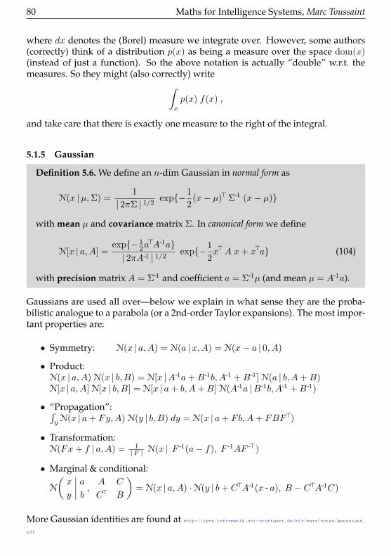
80 Maths for Intelligence Systems, Marc Toussaint
where dx denotes the (Borel) measure we integrate over. However, some authors(correctly) think of a distribution p(x) as being a measure over the space dom(x)(instead of just a function). So the above notation is actually “double” w.r.t. themeasures. So they might (also correctly) write∫
x
p(x) f(x) ,
and take care that there is exactly one measure to the right of the integral.
5.1.5 Gaussian
Definition 5.6. We define an n-dim Gaussian in normal form as
N(x |µ,Σ) =1
| 2πΣ | 1/2exp−1
2(x− µ)>Σ-1 (x− µ)
with mean µ and covariance matrix Σ. In canonical form we define
N[x | a,A] =exp− 1
2a>A-1a
| 2πA-1 | 1/2exp−1
2x>A x+ x>a (104)
with precision matrix A = Σ-1 and coefficient a = Σ-1µ (and mean µ = A-1a).
Gaussians are used all over—below we explain in what sense they are the proba-bilistic analogue to a parabola (or a 2nd-order Taylor expansions). The most impor-tant properties are:
• Symmetry: N(x | a,A) = N(a |x,A) = N(x− a | 0, A)
• Product:N(x | a,A) N(x | b, B) = N[x |A-1a+B-1b, A-1 +B-1] N(a | b, A+B)N[x | a,A] N[x | b, B] = N[x | a+ b, A+B] N(A-1a |B-1b, A-1 +B-1)
• “Propagation”:∫yN(x | a+ Fy,A) N(y | b, B) dy = N(x | a+ Fb,A+ FBF>)
• Transformation:N(Fx+ f | a,A) = 1
|F | N(x | F -1(a− f), F -1AF ->)
• Marginal & conditional:
N
(x
y
∣∣∣∣ ab , A C
C> B
)= N(x | a,A) ·N(y | b+ C>A-1(x - a), B − C>A-1C)
More Gaussian identities are found at http://ipvs.informatik.uni-stuttgart.de/mlr/marc/notes/gaussians.

Maths for Intelligence Systems, Marc Toussaint 81
Example 5.1 (ML estimator of the mean of a Gaussian). Assume we have dataD = x1, .., xn, each xi ∈ Rn, with likelihood
P (D |µ,Σ) =∏iN(xi |µ,Σ)
argmaxµ
P (D |µ,Σ) =1
n
n∑i=1
xi
argmaxΣ
P (D |µ,Σ) =1
n
n∑i=1
(xi − µ)(xi − µ)>
Assume we are initially uncertain about µ (but know Σ). We can express thisuncertainty using again a Gaussian N[µ | a,A]. Given data we have
P (µ |D) ∝ P (D |µ,Σ) P (µ) =∏iN(xi |µ,Σ) N[µ | a,A]
=∏iN[µ |Σ-1xi,Σ
-1] N[µ | a,A] ∝ N[µ |Σ-1∑i xi, nΣ-1 +A]
Note: in the limit A→ 0 (uninformative prior) this becomes
P (µ |D) = N(µ | 1
n
∑i
xi,1
nΣ)
which is consistent with the Maximum Likelihood estimator
5.1.6 “Particle distribution”
Usually, “particles” are not listed as standard continuous distribution. However Ithink they should be. They’re heavily used in several contexts, especially as ap-proximating other distributions in Monte Carlo methods and particle filters.
Definition 5.7 (Dirac or δ-distribution). In distribution theory it is proper to de-fine a distribution δ(x) that is the derivative of the Heavyside step functionH(x),
δ(x) =∂
∂xH(x) , H(x) = [x ≥ 0] .
It is akward to think of δ(x) as a normal function, as it’d be “infinite” at zero.But at least we understand that is has the properties
δ(x) = 0 everywhere except at x = 0 ,
∫δ(x) dx = 1 .
I sometimes call the Dirac distribution also a point particle: it has all its unit “mass”concentrated at zero.

82 Maths for Intelligence Systems, Marc Toussaint
Definition 5.8 (Particle Distribution). We define a particle distribution q(x) asa mixture of Diracs,
q(x) :=
N∑i=1
wi δ(x− xi) ,
which is parameterized by the number N , the locations xiNi=1, xi ∈ Rn, andthe normalized weights wiNi=1, wi ∈ R, ||w||1 = 1 of the N particles.
We say that a particle distribution q(x) approximates another distribution p(x) ifffor any (smooth) f
〈f(x)〉p =
∫x
f(x)p(x)dx ≈∑Ni=1 wif(xi)
Note the generality of this statement! f could be anything, it could be any featuresof the variable x, like coordinates of x, or squares, or anything. So basically thisstatement says, whatever you might like to estimate about p, you can approximateit based on the particles q.
Computing particle approximations of comples (non-analytical, non-tracktable) dis-tributions p is a core challenge in many fields. The true p could for instance bea distributions over games (action sequences). The approximation q could for in-stance be samples generated with Monte Carlo Tree Search (MCTS). The tutorial AnIntroduction to MCMC for Machine Learning www.cs.ubc.ca/˜nando/papers/mlintro.pdf gives an excellent introduction. Here are some illustrations of whatit means to approximate some p by particles q, taken from this tutorial. The blackline is p, histograms illustrate the particles q by showing how many of (uniformlyweighted) particles fall into a bin:

Maths for Intelligence Systems, Marc Toussaint 83
(from de Freitas et al.)
5.2 Between probabilities and optimization: neg-log-probabilities,exp-neg-energies, exponential family, Gibbs and Boltzmann
There is a natural relation between probabilities and “energy” (or “error”). Namely,if p(x) denotes a probability for every possible value of x, and E(x) denotes anenergy for state x—or an error one assigns to choosing x—then a natural relation is
p(x) = e−E(x) , E(x) = − log p(x) .
Why is that? First, outside the context of physics it is perfectly fair to just defineaxiomatically an energy E(x) as neg-log-probability. But let me try to give somemore arguments for why this is a useful definition.
Let assume we have p(x). We want to find a quantity, let’s call it error E(x), whichis a function of p(x). Intuitively, if a certain value x1 is more likely than another,p(x1) > p(x2), then picking x1 should imply less error, E(x1) < E(x2) (Axiom 1).Further, when we have two independent random variables x and y, probabilitiesare multiplicative, p(x, y) = p(x)p(y). We require axiomatically that error is addi-tive, E(x, y) = E(x) + E(y). From both follows that E needs to be some logarithmof p!
The same argument, now more talking about energy: Assume we have two inde-pendent (physical) systems x and y. p(x, y) = p(x)p(y) is the probability to find
84 Maths for Intelligence Systems, Marc Toussaint
them in certain states. We axiomatically require that energy is additive, E(x, y) =E(x) + E(y). Again, E needs to be some logarithm of p. In the context of physics,what could be questioned is “why is p(x) a function of E(x) in the first place?”.Well, that is much harder to explain and really is a question about statistical physics.Wikipedia under keywords “Maxwell-Boltzmann statistics” and “Derivation frommicrocanonical ensemble” gives an answer. Essentially the argument is a follows:Given many many molecules in a gas, each of which can have a different energyei. The total energy E =
∑ni=1 ei must be conserved. What is the distribution over
energy levels that has the most microstates? The answer is the Boltzmann distri-bution. (And why do we, in nature, find energy distributions that have the mostmicrostates? Because these are most likely.)
Bottom line is: p(x) = e−E(x), probabilities are multiplicative, energies or errorsadditive.
Let me state some fact just to underline how useful this way of thinking is:
• Given an energy function E(x), its Boltzmann distribution is defined as
p(x) = e−E(x).
This is sometimes also called Gibbs distribution.
• In machine learning, when data D is given and we have some model β, wetypically try to maximize the likelihood p(D|β). This is equivalent to mini-mizing the neg-log-likelihood
L(β) = − log p(D|β) .
This neg-log-likelihood is a typical measure for error of the model. And thiserror is additive w.r.t. the data, whereas the likelihood is multiplicative, fittingperfectly to the above discussion.
• The Gaussian distribution p(x) ∝ exp− 12 ||x − µ||
2/σ2 is related to the errorE(x) = 1
2 ||x − µ||2/σ2, which is nothing but the squared error with the pre-
cision matrix as metric. That’s why squared error measures (classical regres-sion) and Gaussian distributions (e.g., Bayesian Ridge regression) are directlyrelated.
A Gaussian is the probabilistic analoque to a parabola.
• The exponential family is defined as
p(x|β) = h(x)g(β) expβ>φ(x)
Often h(x) = 1, so let’s neglect this for now. The key point is that the energyis linear in the features φ(x). This is exactly how discriminative functions (forclassification in Machine learning) are typically formulated.
Maths for Intelligence Systems, Marc Toussaint 85
In the continuous case, the features φ(x) are often chosen as basis polynomials—just as in polynomial regression. Then, β are the coefficients of the energypolynomial and the exponential family is just the probabilistic analogue tothe space of polynomials.
• When we have many variables x1, .., xn, the structure of a cost function overthese variables can often be expressed as being additive in terms: f(x1, .., xn) =∑i φi(x∂i) where ∂i denotes the ith group of variables. The respective Boltz-
mann distribution is a factor graph p(x1, .., xn) ∝∏i fi(x∂i) = exp
∑i βiφi(x∂i)
where ∂i denotes the
So, factor graphs are the probabilistic analoque to additive functions.
• − log p(x) is also the “optimal” coding length you should assign to a symbolx.
Entropy is expected error: H[p] =∑x−p(x) log p(x) = 〈− log p(x)〉p(x), where
p itself it used to take the expectation.
Assume you use a “wrong” distribution q(x) to decide on the coding length ofsymbols drawn from p(x). The expected length of an encoding is
∫xp(x)[− log q(x)] ≥
H(p).
The Kullback-Leibler divergence is the difference:
D(p∣∣∣∣ q) =
∫x
p(x) logp(x)
q(x)≥ 0
Proof of inequality, using the Jenson inequality:
−∫x
p(x) logq(x)
p(x)≥ − log
∫x
p(x)q(x)
p(x)= 0
So, my message is that probabilities and error measures are naturally related. How-ever, in the first case we typically do inference, in the second we optimize. Let’sdiscuss the relation between inference and optimization a bit more. For instance,given data D and parameters β, we may define
Definition 5.9 (ML, MAP, and Bayes estimate). Given dataD and a parametericmodel p(D|β), we define
• Maximum likelihood (ML) parameter estimate:
βML := argmaxβ P (D|β)
• Maximum a posteriori (MAP) parameter estimate:
βMAP = argmaxβ P (β|D)
• Bayesian parameter estimate:
P (β|D) ∝ P (D|β) P (β)
86 Maths for Intelligence Systems, Marc Toussaint
used for Bayesian prediction:P (prediction|D) =∫βP (prediction|β)P (β|D)
Both, the MAP and the ML estimates are really just optimization problems.
The Bayesian parameter estimateP (β|D), which can then be used to do fully Bayesianprediction, is in principle different. However, in practise also here optimization is acore tool for estimating such distributions if they cannot be given analytically. Thisis described next.
5.3 Information, Entropie & Kullback-Leibler
Consider the following problem. We have data drawn i.i.d. from p(x) where x ∈X in some discrete space X . Let’s call every x a word. The problem is to find amapping from words to codes, e.g. binary codes c : X → 0, 1∗. The optimalsolution is in principle simple: Sort all possible words in a list, ordered by p(x)with more likely words going first; write all possible binary codes in another list,with increasing code lengths. Match the two lists, and this is the optimal encoding.
Let’s try to get a more analytical grip of this: Let l(x) = |c(x)| be the actual codelength assigned to word x, which is an integer value. Let’s define
q(x) =1
Z2−l(x)
with the normalization constrant Z =∑x 2−l(x). Then we have∑
x∈Xp(x)[− log2 q(x)] = −
∑x
p(x) log 2−l(x) +∑x
p(x) logZ
=∑x
p(x)l(x) + logZ .
What about logZ? Let l-1(s) be the set of words that have been assigned codes oflength l. There can only be a limited number of words encoded with a given length.For instance, |L-1(1)|must not be greater than 2, |L-1(2)|must not be greater than 4,and |l-1(s)|must not be greater than 2l. We have
∀s :∑x∈X
[l(x) = s] ≤ 2s
∀s :∑x∈X
[l(x) = s]2−s ≤ 1
∀s :∑x∈X
2−l(x) ≤ 1
However, this way of thinking is ok for separated codes. If such codes would be ina continuous stream of bits you’d never know where a code starts or ends. Prefix
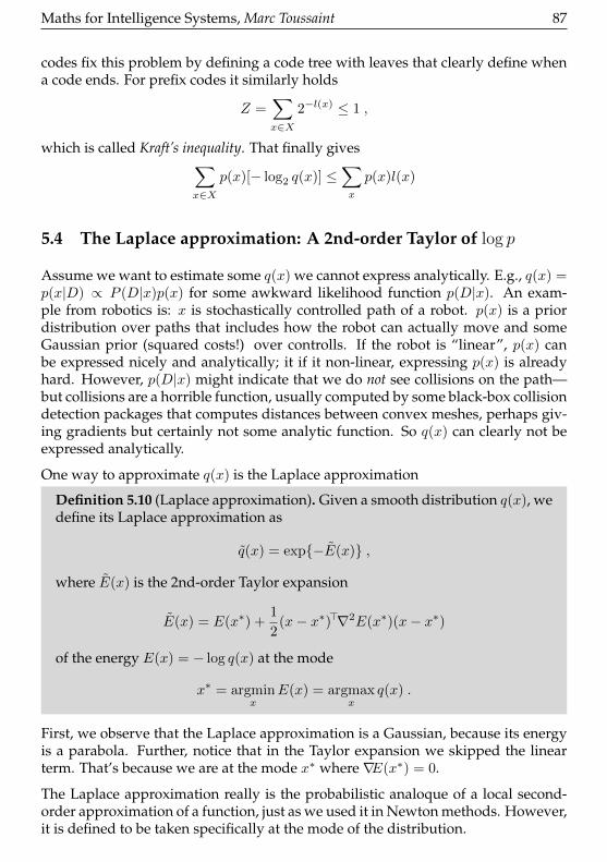
Maths for Intelligence Systems, Marc Toussaint 87
codes fix this problem by defining a code tree with leaves that clearly define whena code ends. For prefix codes it similarly holds
Z =∑x∈X
2−l(x) ≤ 1 ,
which is called Kraft’s inequality. That finally gives∑x∈X
p(x)[− log2 q(x)] ≤∑x
p(x)l(x)
5.4 The Laplace approximation: A 2nd-order Taylor of log p
Assume we want to estimate some q(x) we cannot express analytically. E.g., q(x) =p(x|D) ∝ P (D|x)p(x) for some awkward likelihood function p(D|x). An exam-ple from robotics is: x is stochastically controlled path of a robot. p(x) is a priordistribution over paths that includes how the robot can actually move and someGaussian prior (squared costs!) over controlls. If the robot is “linear”, p(x) canbe expressed nicely and analytically; it if it non-linear, expressing p(x) is alreadyhard. However, p(D|x) might indicate that we do not see collisions on the path—but collisions are a horrible function, usually computed by some black-box collisiondetection packages that computes distances between convex meshes, perhaps giv-ing gradients but certainly not some analytic function. So q(x) can clearly not beexpressed analytically.
One way to approximate q(x) is the Laplace approximation
Definition 5.10 (Laplace approximation). Given a smooth distribution q(x), wedefine its Laplace approximation as
q(x) = exp−E(x) ,
where E(x) is the 2nd-order Taylor expansion
E(x) = E(x∗) +1
2(x− x∗)>∇2E(x∗)(x− x∗)
of the energy E(x) = − log q(x) at the mode
x∗ = argminx
E(x) = argmaxx
q(x) .
First, we observe that the Laplace approximation is a Gaussian, because its energyis a parabola. Further, notice that in the Taylor expansion we skipped the linearterm. That’s because we are at the mode x∗ where∇E(x∗) = 0.
The Laplace approximation really is the probabilistic analoque of a local second-order approximation of a function, just as we used it in Newton methods. However,it is defined to be taken specifically at the mode of the distribution.

88 Maths for Intelligence Systems, Marc Toussaint
Now, computing x∗ is a classical optimization problem x∗ = argminxE(x) whichone might ideally solve using Newton methods. These Newton methods anywaycompute the local Hessian ofE(x) in every step—at the optimum we therefore havethe Hessian already, which is then the precision matrix of our Gaussian.
The Laplace approximation is nice, very efficient to use, e.g., in the context of op-timal control and robotics. While we can use the expressive power of probabilitytheory to formalize the problem, the Laplace approximation brings us computa-tionally back to efficient optimization methods.
5.5 Variational Inference
Another reduction of inference to optimization is variational inference.
Definition 5.11 (variational inference). Given a distribution p(x), and a param-eterized family of distributions q(x|β), the variational approximation of p(x) isdefined as
argminq
D(q∣∣∣∣ p)
5.6 The Fisher information metric: 2nd-order Taylor of the KLD
Recall our notion of steepest descent—it depends on the metric in the space!
Consider the space of probability distributions p(x;β) with parameters β. We thinkof every p(x;β) as a point in the space and wonder what metric is useful to comparetwo points p(x;β1) and p(x;β2). Let’s take the KLD
TODO
: Let p ∈ ΛX , that is, p is a probability distribution over the space X . Further,let θ ∈ Rn and θ 7→ p(θ) is some parameterization of the probability distribution.Then the derivative dθp(θ) ∈ TpΛX is a vector in the tangent space of ΛX . Now, forsuch vectors, for tangent vectors of the space of probability distributions, there is ageneric metric, the Fisher metric: [TODO: move to ’probabilities’ section]
5.7 Examples and Exercises
Note: These exercises are for ’extra credits’. We’ll discuss them on Thu, 21th Jan.
Maths for Intelligence Systems, Marc Toussaint 89
5.7.1 Maximum Entropy and Maximum Likelihood
(These are taken from MacKay’s book Information Theory..., Exercise 22.12 & .13)
a) Assume that a random variable x with discrete domain dom(x) = X comes froma probability distribution of the form
P (x |w) =1
Z(w)exp
[ d∑k=1
wkfk(x)],
where the functions fk(x) are given, and the parameters w ∈ Rd are not known. Adata set D = xini=1 of n points x is supplied. Show by differentiating the log like-lihood logP (D|w) =
∑ni=1 logP (xi|w) that the maximum-likelihood parameters
w∗ = argmaxw logP (D|w) satisfy
∑x∈X
P (x |w∗) fk(x) =1
n
n∑i=1
fk(xi)
where the left-hand sum is over all x, and the right-hand sum is over the datapoints. A shorthand for this result is that each function-average under the fittedmodel must equal the function-average found in the data:
〈fk〉P (x |w∗) = 〈fk〉D
b) When confronted by a probability distribution P (x) about which only a few factsare known, the maximum entropy principle (MaxEnt) offers a rule for choosing adistribution that satisfies those constraints. According to MaxEnt, you should selectthe P (x) that maximizes the entropy
H(P ) = −∑x
P (x) logP (x)
subject to the constraints. Assuming the constraints assert that the averages of cer-tain functions fk(x) are known, i.e.,
〈fk〉P (x) = Fk ,
show, by introducing Lagrange multipliers (one for each constraint, including nor-malization), that the maximum-entropy distribution has the form
PMaxEnt(x) =1
Zexp
[∑k
wk fk(x)]
where the parameters Z and wk are set such that the constraints are satisfied. Andhence the maximum entropy method gives identical results to maximum likelihoodfitting of an exponential-family model.
90 Maths for Intelligence Systems, Marc Toussaint
Note: The exercise will take place on Tue, 2nd Feb. Hung will also prepare howmuch ‘votes’ you collected in the exercises.
5.7.2 Maximum likelihood and KL-divergence
Assume we have a very large data set D = xini=1 of samples xi ∼ q(x) from somedata distribution q(x). Using this data set we can approximate any expectation
〈f〉q =∑x
q(x)f(x) ≈n∑i=1
f(xi) .
Assume we have a parameteric family of distributions p(x|β) and would find theMaximum Likelihood (ML) parameter β∗ = argmaxβ p(D|β). Express this MLproblem as a KL-divergence minimization.
5.7.3 Laplace Approximation
In the context of so-called “Gaussian Process Classification” the following problemarises (we neglect dependence on x here): We have a real-valued RV f ∈ R withprior P (f) = N(f |µ, σ2). Further we have a Boolean RV y ∈ 0, 1with conditionalprobability
P (y=1 | f) = σ(f) =ef
1 + ef.
The function σ is called sigmoid funtion, and f is a discriminative value whichpredicts y = 1 if it is very positive, and y = 0 if it is very negative. The sigmoidfunction has the property
∂
∂fσ(f) = σ(f) (1− σ(f)) .
Given that we observed y = 1 we want to compute the posterior P (f | y=1), whichcannot be expressed analytically. Provide the Laplace approximation of this poste-rior.
(Bonus) As an alternative to the sigmoid function σ(f), we can use the probit func-tion φ(z) =
∫ z−∞N(x|0, 1) dx to define the likelihood P (y=1 | f) = φ(f). Now how
can the posterior P (f | y=1) be approximated?
Maths for Intelligence Systems, Marc Toussaint 91
5.7.4 Learning = Compression
In a very abstract sense, learning means to model the distribution p(x) for givendata D = xini=1. This is literally the case for unsupervised learning; regression,classification and graphical model learning could be viewed as specific instances ofthis where x factores in several random variables, like input and output.
Show in which sense the problem of learning is equivalent to the problem of com-pression.
5.7.5 A gzip experiment
Get three text files from the Web, approximately equal length, mostly text (no equa-tions or stuff). Two of them should be in English, the third in Frensh. (Alternatively,perhaps, not sure if it’d work, two of them on a very similar topic, the third on avery different.)
How can you use gzip (or some other compression tool) to estimate the mutualinformation between every pair of files? How can you ensure some “normalized”measures which do not depend too much on the absolute lengths of the text? Doit and check whether in fact you find that two texts are similar while the third isdifferent.
(Extra) Lempel-Ziv algorithms (like gzip) need to build a codebook on the fly. Howdoes that fit into the picture?
5.7.6 Maximum Entropy and ML
(These are taken from MacKay’s book Information Theory..., Exercise 22.12 & .13)
a) Assume that a random variable x with discrete domain dom(x) = X comes froma probability distribution of the form
P (x |w) =1
Z(w)exp
[ d∑k=1
wkfk(x)],
where the functions fk(x) are given, and the parameters w ∈ Rd are not known. Adata set D = xini=1 of n points x is supplied. Show by differentiating the log like-lihood logP (D|w) =
∑ni=1 logP (xi|w) that the maximum-likelihood parameters
w∗ = argmaxw logP (D|w) satisfy
∑x∈X
P (x |w∗) fk(x) =1
n
n∑i=1
fk(xi)

92 Maths for Intelligence Systems, Marc Toussaint
where the left-hand sum is over all x, and the right-hand sum is over the datapoints. A shorthand for this result is that each function-average under the fittedmodel must equal the function-average found in the data:
〈fk〉P (x |w∗) = 〈fk〉D
b) When confronted by a probability distribution P (x) about which only a few factsare known, the maximum entropy principle (MaxEnt) offers a rule for choosing adistribution that satisfies those constraints. According to MaxEnt, you should selectthe P (x) that maximizes the entropy
H(P ) = −∑x
P (x) logP (x)
subject to the constraints. Assuming the constraints assert that the averages of cer-tain functions fk(x) are known, i.e.,
〈fk〉P (x) = Fk ,
show, by introducing Lagrange multipliers (one for each constraint, including nor-malization), that the maximum-entropy distribution has the form
PMaxEnt(x) =1
Zexp
[∑k
wk fk(x)]
where the parameters Z and wk are set such that the constraints are satisfied. Andhence the maximum entropy method gives identical results to maximum likelihoodfitting of an exponential-family model.
A Gaussian identities
DefinitionsWe define a Gaussian over x with mean a and covariance matrix A as the function
N(x | a,A) =1
|2πA|1/2exp−1
2(x-a)>A-1 (x-a) (105)
with property N(x | a,A) = N(a| x,A). We also define the canonical form withprecision matrix A as
N[x | a,A] =exp− 1
2a>A-1a
|2πA-1|1/2exp−1
2x>A x+ x>a (106)
with properties
N[x | a,A] = N(x |A-1a,A-1) (107)
Maths for Intelligence Systems, Marc Toussaint 93
N(x | a,A) = N[x |A-1a,A-1] . (108)
Non-normalized Gaussian
N(x, a,A) = |2πA|1/2 N(x|a,A) (109)
= exp−1
2(x-a)>A-1 (x-a) (110)
Matrices [matrix cookbook: http://www.imm.dtu.dk/pubdb/views/edoc_download.php/3274/pdf/imm3274.pdf]
(A-1 +B-1)-1 = A (A+B)-1 B = B (A+B)-1 A (111)
(A-1 −B-1)-1 = A (B-A)-1 B (112)
∂x|Ax| = |Ax| tr(A-1x ∂xAx) (113)
∂xA-1x = −A-1
x (∂xAx) A-1x (114)
(A+ UBV )-1 = A-1 −A-1U(B-1 + V A-1U)-1V A-1 (115)
(A-1 +B-1)-1 = A−A(B +A)-1A (116)
(A+ J>BJ)-1J>B = A-1J>(B-1 + JA-1J>)-1 (117)
(A+ J>BJ)-1A = I− (A+ J>BJ)-1J>BJ (118)
(115)=Woodbury; (117,118) holds for pos def A and B
Derivatives
∂xN(x|a,A) = N(x|a,A) (−h>) , h := A-1(x-a) (119)∂θN(x|a,A) = N(x|a,A) ·[− h>(∂θx) + h>(∂θa)− 1
2tr(A-1 ∂θA) +
1
2h>(∂θA)h
](120)
∂θN[x|a,A] = N[x|a,A][− 1
2x>∂θAx+
1
2a>A-1∂θAA
-1a
+ x>∂θa− a>A-1∂θa+1
2tr(∂θAA
-1)]
(121)
∂θNx(a,A) = Nx(a,A) ·[h>(∂θx) + h>(∂θa) +
1
2h>(∂θA)h
](122)
ProductThe product of two Gaussians can be expressed as
N(x | a,A) N(x | b, B)
= N[x |A-1a+B-1b, A-1 +B-1] N(a | b, A+B) , (123)

94 Maths for Intelligence Systems, Marc Toussaint
= N(x |B(A+B)-1a+A(A+B)-1b, A(A+B)-1B) N(a | b, A+B) , (124)N[x | a,A] N[x | b, B]
= N[x | a+ b, A+B] N(A-1a |B-1b, A-1 +B-1) (125)
= N[x| . . . ] N[A-1a |A(A+B)-1b, A(A+B)-1B] (126)
= N[x| . . . ] N[A-1a | (1-B(A+B)-1) b, (1-B(A+B)-1) B] , (127)N(x | a,A) N[x | b, B]
= N[x |A-1a+ b, A-1 +B] N(a |B-1b, A+B-1) (128)
= N[x| . . . ] N[a | (1-B(A-1+B)-1) b, (1-B(A-1+B)-1) B] (129)
Convolution∫xN(x | a,A) N(y − x | b, B) dx = N(y | a+ b, A+B) (130)
Division
N(x|a,A)/N(x|b, B) = N(x|c, C)
/N(c|b, C +B)
C -1c = A-1a−B-1b
C -1 = A-1 −B-1 (131)
N[x|a,A]/N[x|b, B] ∝ N[x|a− b, A−B] (132)
ExpectationsLet x ∼ N(x | a,A),
Exg(x) :=∫xN(x | a,A) g(x) dx (133)
Exx = a , Exxx>= A+ aa> (134)Exf + Fx = f + Fa (135)
Exx>x = a>a+ tr(A) (136)
Ex(x-m)>R(x-m) = (a-m)>R(a-m) + tr(RA) (137)
Transformation Linear transformations imply the following identities,
N(x | a,A) = N(x+ f | a+ f, A) , N(x | a,A) = |F | N(Fx |Fa, FAF>)
(138)
N(Fx+ f | a,A) =1
|F |N(x | F -1(a− f), F -1AF ->) (139)
=1
|F |N[x | F>A-1(a− f), F>A-1F ] , (140)
Maths for Intelligence Systems, Marc Toussaint 95
N[Fx+ f | a,A] =1
|F |N[x | F>(a−Af), F>AF ] . (141)
“Propagation” (propagating a message along a coupling, using eqs (123) and(129), respectively)
∫yN(x | a+ Fy,A) N(y | b, B) dy = N(x | a+ Fb,A+ FBF>) (142)∫
yN(x | a+ Fy,A) N[y | b, B] dy = N[x | (F ->-K)(b+BF -1a), (F ->-K)BF -1] ,
(143)
K = F ->B(F ->A-1F -1+B)-1 (144)
marginal & conditional:
N(x | a,A) N(y | b+ Fx,B) = N
(x
y
∣∣∣∣ a
b+ Fa,
A A>F>
FA B+FA>F>
)(145)
N
(x
y
∣∣∣∣ ab , A C
C> B
)= N(x | a,A) ·N(y | b+ C>A-1(x-a), B − C>A-1C)
(146)
N[x | a,A] N(y | b+ Fx,B) = N
[x
y
∣∣∣∣ a+ F>B-1b
B-1b,A+ F>B-1F −F>B-1
−B-1F B-1
](147)
N[x | a,A] N[y | b+ Fx,B] = N
[x
y
∣∣∣∣ a+ F>B-1b
b,A+ F>B-1F −F>
−F B
](148)
N
[x
y
∣∣∣∣ ab , A C
C> B
]= N[x | a− CB-1b, A− CB-1C>] ·N[y | b− C>x,B]
(149)∣∣∣∣∣ A C
D B
∣∣∣∣∣ = |A| |B| = |A| |B| ,whereA = A− CB-1D
B = B −DA-1C
(150)[A C
D B
]-1
=
[A-1 −A-1CB-1
−B-1DA-1 B-1
](151)
=
[A-1 −A-1CB-1
−B-1DA-1 B-1
](152)

96 Maths for Intelligence Systems, Marc Toussaint
pair-wise belief We have a messageα(x) = N[x|s, S], transitionP (y|x) = N(y|Ax+a,Q), and a message β(y) = N[y|v, V ], what is the belief b(y, x) = α(x)P (y|x)β(y)?
b(y, x) = N[x|s, S] N(y|Ax+ a,Q-1) N[y|v, V ] (153)
= N
[x
y
∣∣∣∣ s0 , S 0
0 0
]N
[x
y
∣∣∣∣ A>Q-1a
Q-1a,A>Q-1A −A>Q-1
−Q-1A Q-1
]N
[x
y
∣∣∣∣ 0
v,
0 0
0 V
](154)
∝ N
[x
y
∣∣∣∣ s+A>Q-1a
v +Q-1a,S +A>Q-1A −A>Q-1
−Q-1A V +Q-1
](155)
Entropy
H(N(a,A)) =1
2log |2πeA| (156)
Kullback-Leibler divergence
p = N(x|a,A) , q = N(x|b, B) , n = dim(x) , D(p∣∣∣∣ q) =
∑x
p(x) logp(x)
q(x)
(157)
2 D(p∣∣∣∣ q) = log
|B||A|
+ tr(B-1A) + (b− a)>B-1(b− a)− n (158)
4 Dsym(p∣∣∣∣ q) = tr(B-1A) + tr(A-1B) + (b− a)>(A-1 +B-1)(b− a)− 2n (159)
λ-divergence
2 Dλ
(p∣∣∣∣ q) = λ D
(p∣∣∣∣λp+ (1−λ)q
)+ (1−λ) D
(p∣∣∣∣ (1−λ)p+ λq
)(160)
For λ = .5: Jensen-Shannon divergence.
Log-likelihoods
logN(x|a,A) = −1
2
[log|2πA|+ (x-a)>A-1 (x-a)
](161)
logN[x|a,A] = −1
2
[log|2πA-1|+ a>A-1a+ x>Ax− 2x>a
](162)∑
x
N(x|b, B) logN(x|a,A) = −D(N(b, B)
∣∣∣∣N(a,A))−H(N(b, B)) (163)

Maths for Intelligence Systems, Marc Toussaint 97
Mixture of Gaussians Collapsing a MoG into a single Gaussian
argminb,B
D(∑
i
pi N(ai, Ai)∣∣∣∣N(b, B)
)(164)
=(b =
∑i
piai , B =∑i
pi(Ai + aia>i − b b>)
)(165)
B 3D geometry basics (for robotics)
This document introduces to some basic geometry, focussing on 3D transforma-tions, and introduces proper conventions for notation. There exist one-to-one im-plementations of the concepts and equations in libORS.
B.1 Rotations
There are many ways to represent rotations in SO(3). We restrict ourselves to threebasic ones: rotation matrix, rotation vector, and quaternion. The rotation vector isalso the most natural representation for a “rotation velocity” (angular velocities).Euler angles or raw-pitch-roll are an alternative, but they have singularities and Idon’t recommend using them in practice.
A rotation matrix is a matrix R ∈ R3×3 which is orthonormal (columns and rowsare orthogonal unit vectors, implying determinant 1). While a 3×3 matrix has9 degrees of freedom (DoFs), the constraint of orthogonality and determinant1 constraints this: The set of rotation matrices has only 3 DoFs (∼ the local Liealgebra is 3-dim).
The application of R on a vector x is simply the matrix-vector product Rx.
Concatenation of two rotations R1 and R2 is the normal matrix-matrix prod-uct R1R2.
Inversion is the transpose, R-1 = R>.
A rotation vector is an unconstraint vector w ∈ R3. The vector’s direction w =w|w| determines the rotation axis, the vector’s length |w| = θ determins therotation angle (in radians, using the right thumb convention).
The application of a rotation described by w ∈ R3 on a vector x ∈ R3 is givenas (Rodrigues’ formula)
w · x = cos θ x+ sin θ (w × x) + (1− cos θ) w(w>x) (166)
where θ = |w| is the rotation angle and w = w/θ the unit length rotation axis.
The inverse rotation is described by the negative of the rotation vector.
98 Maths for Intelligence Systems, Marc Toussaint
Concatenation is non-trivial in this representation and we don’t discuss ithere. In practice, a rotation vector is first converted to a rotation matrix orquaternion.
Convertion to a matrix: For every vectorw ∈ R3 we define its skew symmetricmatrix as
w =
0 −w3 w2
w3 0 −w1
−w2 w1 0
. (167)
Note that such skew-symmetric matrices are related to the cross product: w×v = w v, where the cross product is rewritten as a matrix product. The rotationmatrix R(w) that corresponds to a given rotation vector w is:
R(w) = exp(w) (168)
= cos θ I + sin θ w/θ + (1− cos θ) ww>/θ2 (169)
The exp function is called exponential map (generating a group element (=ro-tation matrix) via an element of the Lie algebra (=skew matrix)). The otherformular is called Rodrigues’ formular: the first term is a diagonal matrix (Iis the 3D identity matrix), the second terms the skew symmetric part, the lastterm the symmetric part (ww> is also called outper product).
Angular velocity & derivative of a rotation matrix: We represent angular veloci-ties by a vectorw ∈ R3, the directionw determines the rotation axis, the length|w| is the rotation velocity (in radians per second). When a body’s orientationat time t is described by a rotation matrixR(t) and the body’s angular velocityis w, then
R(t) = w R(t) . (170)
(That’s intuitive to see for a rotation about the x-axis with velocity 1.) Someinsights from this relation: Since R(t) must always be a rotation matrix (ful-fill orthogonality and determinant 1), its derivative R(t) must also fulfill cer-tain constraints; in particular it can only live in a 3-dimensional sub-space. Itturns out that the derivative R of a rotation matrix R must always be a skewsymmetric matrix w times R – anything else would be inconsistent with thecontraints of orthogonality and determinant 1.
Note also that, assuming R(0) = I , the solution to the differential equationR(t) = w R(t) can be written as R(t) = exp(tw), where here the exponentialfunction notation is used to denote a more general so-called exponential map,as used in the context of Lie groups. It also follows thatR(w) from (168) is therotation matrix you get when you rotate for 1 second with angular velocitydescribed by w.
Quaternion (I’m not describing the general definition, only the “quaternion to rep-resent rotation” definition.) A quaternion is a unit length 4D vector r ∈ R4;
Maths for Intelligence Systems, Marc Toussaint 99
the first entry r0 is related to the rotation angle θ via r0 = cos(θ/2), thelast three entries r ≡ r1:3 are related to the unit length rotation axis w viar = sin(θ/2) w.The inverse of a quaternion is given by negating r, r-1 = (r0,−r) (or, alterna-tively, negating r0).The concatenation of two rotations r, r′ is given as the quaternion product
r r′ = (r0r′0 − r>r′, r0r
′ + r′0r + r′ × r) (171)
The application of a rotation quaternion r on a vector x can be expressed byconverting the vector first to the quaternion (0, x), then computing
r · x = (r (0, x) r-1)1:3 , (172)
I think a bit more efficient is to first convert the rotation quaternion r to theequivalent rotation matrix R, as given by
R =
1− r22 − r33 r12 − r03 r13 + r02
r12 + r03 1− r11 − r33 r23 − r01
r13 − r02 r23 + r01 1− r11 − r22
rij := 2rirj . (173)
(Note: In comparison to (168) this does not require to compute a sin or cos.)Inversely, the quaterion r for a given matrix R is
r0 =1
2
√1 + trR (174)
r3 = (R21 −R12)/(4r0) (175)r2 = (R13 −R31)/(4r0) (176)r1 = (R32 −R23)/(4r0) . (177)
Angular velocity→ quaternion velocity Given an angular velocity w ∈ R3 and acurrent quaterion r(t) ∈ R, what is the time derivative r(t) (in analogy toEq. (170))? For simplicity, let’s first assume |w| = 1. For a small time intervalδ, w generates a rotation vector δw, which converts to a quaterion
∆r = (cos(δ/2), sin(δ/2)w) . (178)
That rotation is concatenated LHS to the original quaternion,
r(t+ δ) = ∆r r(t) . (179)
Now, if we take the derivative w.r.t. δ and evaluate it at δ = 0, all the cos(δ/2)terms become − sin(δ/2) and evaluate to zero, all the sin(δ/2) terms becomecos(δ/2) and evaluate to one, and we have
r(t) =1
2(−w>r, r0w + r × w) =
1
2(0, w) r(t) (180)
Here (0, w) ∈ R4 is a four-vector; for |w| = 1 it is a normalized quaternion.However, due to the linearity the equation holds for any w.
100 Maths for Intelligence Systems, Marc Toussaint
Quaternion velocity→ angular velocity The following is relevant when taking thederivative w.r.t. the parameters of a quaternion, e.g., for a ball joint repre-sented as quaternion. Given r, we have
r r-1 =1
2(0, w) r r-1 =
1
2(0, w) (181)
which allows us to read off the angular velocity induced by a change ofquaternion. However, the RHS zero will hold true only iff r is orthogonalto r (where r>r = r0r0 + ˙r>r = 0, see (171)). In case r>r 6= 0, the changein length of the quaterion does not represent any angular velocity; in typicalkinematics engines a non-unit length is ignored. Therefore one first orthogo-nalizes r ← r − r(r>r).
As a special case of application, consider computing the partial derivativew.r.t. quaternion coordinates, where r is the unit vectors e0, .., e3. In this case,the orthogonalization becomes simply ei ← ei − rri and
(ei − rir) r-1 = ei r-1 − ri(1, 0, 0, 0) (182)
wi = 2[ei r-1]1:3 , (183)
where wi is the rotation vector implied by r = ei. In case the original quater-nion r wasn’t normalized (which could be, if a standard optimization algo-rithm searches in the quaternion configuration space), then r actually repre-sents the normalized quaternion r = 1√
r2r, and (due to linearity of the above),
the rotation vector implied by r = ei is
wi =2√r2
[ei r-1]1:3 . (184)
B.2 Transformations
We consider two types of transformations here: either static (translation+rotation),or dynamic (translation+velocity+rotation+angular velocity). The first maps be-tween two static reference frames, the latter between moving reference frames, e.g.between reference frames attached to moving rigid bodies.
B.2.1 Static transformations
Concerning the static transformations, again there are different representations:
A homogeneous matrix is a 4× 4-matrix of the form
T =R t
0 1
(185)
Maths for Intelligence Systems, Marc Toussaint 101
where R is a 3× 3-matrix (rotation in our case) and t a 3-vector (translation).
In homogeneous coordinates, vectors x ∈ R3 are expanded to 4D vectorsx1
∈ R4 by appending a 1.
Application of a transform T on a vector x ∈ R3 is then given as the normalmatrix-vector product
x′ = T · x = Tx
1
=R t
0 1
x
1
=Rx+ t
1
. (186)
Concatenation is given by the ordinary 4-dim matrix-matrix product.
The inverse transform is
T -1 =R t
0 1
-1
=R-1 −R-1t
0 1
(187)
Translation and quaternion: A transformation can efficiently be stored as a pair(t, r) of a translation vector t and a rotation quaternion r. Analogous to theabove, the application of (t, r) on a vector x is x′ = t + r · x; the inverse is(t, r)-1 = (−r-1 ·t, r-1); the concatenation is (t1, r1)(t2, r2) = (t1+r1 ·t2, r1r2).
B.2.2 Dynamic transformations
Just as static transformations map between (static) coordinate frames, dynamictransformations map between moving (inertial) frames which are, e.g., attached tomoving bodies. A dynamic transformation is described by a tuple (t, r, v, w) withtranslation t, rotation r, velocity v and angular velocity w. Under a dynamic trans-form (t, r, v, w) a position and velocity (x, x) maps to a new position and velocity(x′, x′) given as
x′ = t+ r · x (188)x′ = v + w × (r · x) + r · x (189)
(the second term is the additional linear velocity of x′ arising from the angular ve-locity w of the dynamic transform). The concatenation (t, r, v, w) = (t1, r1, v1, w1) (t2, r2, v2, w2) of two dynamic transforms is given as
t = t1 + r1 · t2 (190)v = v1 + w1 × (r1 · t2) + r1 · v2 (191)r = r1 r2 (192)w = w1 + r1 · w2 (193)
102 Maths for Intelligence Systems, Marc Toussaint
For completeness, the footnote9 also describes how accelerations transform, includ-ing the case when the transform itself is accelerating. The inverse (t′, r′, v′, w′) =(t, r, v, w)-1 of a dynamic transform is given as
t′ = −r-1 · t (200)
r′ = r-1 (201)
v′ = r-1 · (w × t− v) (202)
w′ = −r-1 · w (203)
Sequences of transformations by TA→B we denote the transformation from frameA to frameB. The framesA andB can be thought of coordinate frames (tuplesof an offset (in an affine space) and three local orthonormal basis vectors)attached to two bodies A and B. It holds
TA→C = TA→B TB→C (204)
where is the concatenation described above. Let p be a point (rigorously, inthe affine space). We write pA for the coordinate vector of point p relative toframe A; and pB for the coordinate vector of point p relative to frame B. Itholds
pA = TA→B pB . (205)
B.2.3 A note on affine coordinate frames
Instead of the notation TA→B , other text books often use notations such as TAB orTAB . A common question regarding notation TA→B is the following:
The notation TA→B is confusing, since it transforms coordinates from frameB to frame A. Why not the other way around?
9Transformation of accelerations:
v = v1 + w1 × (r1 · t2) + w1 × (w1 × (r1 · t2))+ 2w1 × (r1 · v2) + r1 · v2 (194)
w = w1 + w1 × (r1 · w2) + r1 · w2 (195)
Used identities: for any vectors a, b, c and rotation r:
r · (a× b) = (r · a)× (r · b) (196)
a× (b× c) = b(ac)− c(ab) (197)
∂t(r · a) = w × (r · a) + r · a (198)
∂t(w × a) = w × t+ w × a (199)
Maths for Intelligence Systems, Marc Toussaint 103
I think the notation TA→B is intuitive for the following reasons. The core is tounderstand that a transformation can be thought of in two ways: as a transforma-tion of the coordinate frame itself, and as transformation of the coordinates relative toa coodrinate frame. I’ll first give a non-formal explanation and later more formaldefinitions of affine frames and their transformation.
Think of TW→B as translating and rotating a real rigid body: First, the body islocated at the world origin; then the body is moved by a translation t; then the body
is rotated (around its own center) as described byR. In that sense, TW→B =R t
0 1
describes the “forward” transformation of the body. Consider that a coordinateframe B is attached to the rigid body and a frame W to the world origin. Givena point p in the world, we can express its coordinates relative to the world, pW ,or relative to the body pB . You can convince yourself with simple examples thatpW = TW→B pB , that is, TW→B also describes the “backward” transformation ofbody-relative-coordinates to world-relative-coordinates.
Formally: Let (A, V ) be an affine space. A coordinate frame is a tuple (o, e1, .., en)of an origin o ∈ A and basis vectors ei ∈ V . Given a point p ∈ A, its coordinatesp1:n w.r.t. a coordinate frame (o, e1, .., en) are given implicitly via
p = o+∑
ipiei . (206)
A transformation TW→B is a (“forward”) transformation of the coordinate frameitself:
(oB , eB1 , .., eBn ) = (oW + t, ReW1 , .., ReWn ) (207)
where t ∈ V is the affine translation in A and R the rotation in V . Note that thecoordinates (eBi )W1:n of a basis vector eBi relative to frame W are the columns of R:
eBi =∑j
(eBi )Wj eWj =∑j
RjieWj (208)
Given this transformation of the coordinate frame itself, the coordinates transformas follows:
p = oW +∑i
pWi eWi (209)
p = oB +∑i
pBi eBi (210)
= oW + t+∑i
pBi (ReWi ) (211)
= oW +∑i
tWi eWi +∑j
pBj (ReWj ) (212)
= oW +∑i
tWi eWi +∑j
pBj (∑i
Rij eWi ) (213)
104 Maths for Intelligence Systems, Marc Toussaint
= oW +∑i
[tWi +
∑j
Rij pBj
]eWi (214)
⇒ pWi = tWi +∑j
Rij pBj . (215)
Another way to express this formally: TW→B maps covariant vectors (including“basis vectors”) forward, but contra-variant vectors (including “coordinate vectors”)backward.
B.3 Kinematic chains
In this section we only consider static transformations compost of translation androtation. But given the general concatenation rules above, everything said heregenerealizes directly to the dynamic case.
B.3.1 Rigid and actuated transforms
A actuated kinematic chain with n joints is a series of transformations of the form
TW→1 Q1 T1→2 Q2 T2→3 Q3 · · · (216)
Each Ti-1→i describes so-called “links” (or bones) of the kinematic chain: the rigid(non-actuated) transformation from the i-1th joint to the ith joint. The first TW→1 isthe transformation from world coordinates to the first joint.
Each Qi is the actuated transformation of the joint – usually simply a rotationaround the joint’s x-axis with a specific angle, the so-called joint angle. These jointangles (and therefore each Qi) are actuated and may change over time.
When we control the robot we essentially tell it to actuate its joint so as to changethe joint angles. There are two fundamental computations necessary for control:
(i) For a given n-dimensional vector q ∈ Rn of joint angles, compute the absoluteframes TW→i (world to link transformation) of each link i.
(ii) For a given n-dimensional vector q ∈ Rn of joint angle velocities, computeabsolute (world-relative) velocity and angular velocity of the ith link.
The first problem is solved by “forward chaining” the transformations: we cancompute the absolute transforms TW→i (i.e., the transformation from world to theith link) for each link, namely:
TW→i = TW→i-1 Qi Ti-1→i . (217)
Iterating this for i = 2, .., n we get positions and orientations TW→i of all links inworld coordinates.
The second problem is addressed in the next section.

Maths for Intelligence Systems, Marc Toussaint 105
pk
pj
pi
ai
ak
aj
Figure 6: Illustration for the Jacobian and Hessian.
B.3.2 Jacobian & Hessian
Assume we have computed the absolute position and orientation of each link inan actuated kinematic chain. Then we want to know how a point pWi attached tothe ith frame (and coordinates expressed w.r.t. the world frame W ) changes whenrotating the jth joint. Equally we want to know how some arbitrary vector aWi at-tached to the ith frame (coordinates relative to the world frame W ) rotates whenrotating the jth joint. Let aWj be the unit length rotation axis of the jth joint (which,by convention, is rW→j · (1, 0, 0) if rW→j is the rotation in TW→j). In the follow-ing we drop the superscript W because all coordinates are expressed in the worldframe. Let qj be the joint angle of the jth joint. For the purpose of computing apartial deriviative of something attached to link i w.r.t. the actuation at joint j wecan think of everything inbetween as rigid. Hence, the point and vector Jacobianand Hessian are simply:
dij := pi − pj∂pi∂qj
= aj × dij (218)
∂ai∂qj
= αj × ai (219)
∂2pi∂qj ∂qk
=∂aj∂qk× dij + aj ×
∂dij∂qk
= (ak × aj)× dij + aj × [ak × (pi − pk)− ak × (pj − pk)]
= (ak × aj)× dij + aj × (ak × dij)[using a× (b× c) + b× (c× a) + c× (a× b) = 0
]= ak × (aj × dij) (220)
∂2ai∂qj ∂qk
= (ak × αj)× ai + αj × (ak × ai)
= ak × (αj × ai) (221)

106 Maths for Intelligence Systems, Marc Toussaint
Efficient computation: Assume we have an articulated kinematic tree of links andjoints. We write j < i if joint j is inward from link (or joint) i. Then, for each bodyi consider all inward edges j < i and further inward edges k ≤ j and computeHijk = ∂θj∂θkpi. Note that Hijk is symmetric in j and k – so computing for k ≤ jand copying the rest is sufficient.
References
J. M. Hernandez-Lobato, M. W. Hoffman, and Z. Ghahramani. Predictiveentropy search for efficient global optimization of black-box functions. InZ. Ghahramani, M. Welling, C. Cortes, N. Lawrence, and K. Weinberger,editors, Advances in Neural Information Processing Systems 27, pages 918–926. Curran Associates, Inc., 2014. URL http://papers.nips.cc/paper/5324-predictive-entropy-search-for-efficient-global-optimization-of-black-box-functions.pdf.
D. Jones, M. Schonlau, and W. Welch. Efficient global optimization of expensiveblack-box functions. Journal of Global Optimization, 13:455–492, 1998.
M. Toussaint. A novel augmented lagrangian approach for inequalities and con-vergent any-time non-central updates. e-Print arXiv:1412.4329, 2014.

Maths for Intelligence Systems, Marc Toussaint 107
Exam Tip: These are the headings of all questions that appeared in exams – noguarantee that similar ones might appear. To guess what the question behind sucha heading might be, look up an exercise with similar heading.
– Derivatives
– Vector Spaces
– Inner Product
– Projections
– Fundamental Theorem and SVD
– Eigenvectors
– Singular and Eigenvalues
– Volume
– Linear Robot
– Jacobian
– Taylor expansion
– Lagrangian Method
– Gradient Descent & Newton Method
– KKT
– Log Barrier
– Squared Penalty & Augmented Lagrangian
– Linear Program
– KKT conditions
– Gaussian Distribution
– Laplace Approximation
– Bayesian Reasoning
– Posterior mean of Gaussian
– Acquisition Function
– No Free Lunch

Indexp-norm, 6(dual problem), 57(primal problem), 57
basis, 9Bayes’ Theorem, 78Bayesian parameter estimate:, 85Bayesian prediction: , 86belief MDP, 66BFGS, 50Boltzmann distribution, 84bound constraints, 58
characteristic polynomial, 21column space, 18computation graph, 30conditional, 78conjugate, 50, 79contra-variant, 35convex, 61coordinates, 9covariance, 80covariance matrix, 20covariant, 35cumulative probability distribution, 79
damping, 47determinant, 17diagonalization, 21direct sum, 6domain, 77dual, 13dual space, 10dual variable, 47dual vector, 10
eigendecomposition, 21eigenvector, 21energy is additive, 84Entropy is expected error, 85error is additive, 83Euclidean, 14Expected Improvement (EI), 67
factor graph, 85Fisher metric, 88function network, 30
gradient, 32
Hadamard product, 6Hessian, 33
independent, 78input null space, 18interior point method, 55
Jacobian, 32joint, 78
Kronecker, 5Kronecker delta, 10Kullback-Leibler divergence, 85
Lagrange multiplier, 57Levenberg-Marquardt, 47Limited memory BFGS (L-BFGS), 50linear, 8Linear Program (LP):, 62linearly independent, 9LP in standard form:, 62
marginal, 78matrix, 11matrix convention, 11matrix multiplication, 12Maximum a posteriori (MAP) parame-
ter estimate:, 85Maximum likelihood (ML) parameter
estimate:, 85mean, 80metric tensor, 14mixture, 82mode, 79modified (=approximate) KKT conditions,
60multi-linear, 8
108

Maths for Intelligence Systems, Marc Toussaint 109
orthonormal, 14outer product, 6, 11output null space, 18
particle distribution, 82perfect line search, 50point particle, 81polytope, 63precision, 80Predictive Entropy Search, 67, 68primal-dual space, 58probabilities are multiplicative, 83probability density function (pdf), 79probability distribution, 77, 79probability measure, 77Probability of Improvement (MPI), 67product rule, 78projection, 18
Quadratic Program (QP):, 62Quadratically Constrained QP (QCQP),
62quasiconvex, 61
random variable, 77rank, 17relaxations, 62root, 45row space, 18
saddle point, 33saddle point of the Lagrangian, 56sample space, 77scalar product, 13Slater condition, 58steepest descent, 36strong duality, 58sum-of-squares, 48
tensor product, 11the approximate Hessian is the pullback
of a Euclidean cost feature met-ric, 48
total derivative, 31transpose, 15Trust region method:, 47
unimodal, 61Upper Confidence Bound (UCB), 67
vector, 7vector space, 7volume, 20
Wolfe condition, 44


