Mathematics of Data: From Theory to Computation - epfl.ch
50
Mathematics of Data: From Theory to Computation Prof. Volkan Cevher volkan.cevher@epfl.ch Lecture 7: Deep learning I Laboratory for Information and Inference Systems (LIONS) École Polytechnique Fédérale de Lausanne (EPFL) EE-556 (Fall 2020)
Transcript of Mathematics of Data: From Theory to Computation - epfl.ch

Mathematics of Data: From Theory to Computation
Prof. Volkan [email protected]
Lecture 7: Deep learning ILaboratory for Information and Inference Systems (LIONS)
École Polytechnique Fédérale de Lausanne (EPFL)
EE-556 (Fall 2020)

License Information for Mathematics of Data Slides
I This work is released under a Creative Commons License with the following terms:I Attribution
I The licensor permits others to copy, distribute, display, and perform the work. In return, licensees must give theoriginal authors credit.
I Non-CommercialI The licensor permits others to copy, distribute, display, and perform the work. In return, licensees may not use the
work for commercial purposes – unless they get the licensor’s permission.I Share Alike
I The licensor permits others to distribute derivative works only under a license identical to the one that governs thelicensor’s work.
I Full Text of the License
Mathematics of Data | Prof. Volkan Cevher, [email protected] Slide 2/ 43

Outline
◦ This classI Introduction to Deep LearningI The Deep Learning ParadigmI Challenges in Deep Learning Theory and ApplicationsI Introduction to Generalization error bounds
I Uniform Convergence and Rademacher ComplexityI Generalization in Deep Learning (Part 1)◦ Next classI Generalization in Deep Learning (Part 2)
Mathematics of Data | Prof. Volkan Cevher, [email protected] Slide 3/ 43

Remark about notation
◦ The Deep Learning literature might use a different notation:
Our lectures DL literaturedata/sample a x
label b ybias µ b
weight x,X w,W
Mathematics of Data | Prof. Volkan Cevher, [email protected] Slide 4/ 43

Power of linear classifiers–IProblem (Recall: Logistic regression)Given a sample vector ai ∈ Rd and a binary class label bi ∈ {−1,+1} (i = 1, . . . , n), we define the conditionalprobability of bi given ai as:
P(bi|ai,x) ∝ 1/(1 + e−bi〈x,ai〉),
where x ∈ Rd is some weight vector.
ax
a y
ax
a y
b = + 1b = 1
Figure: Linearly separable versus nonlinearly separable dataset
Mathematics of Data | Prof. Volkan Cevher, [email protected] Slide 5/ 43

Power of linear classifiers–II◦ Lifting dimensions to the rescueI Convex optimization objectiveI Might introduce the curse-of-dimensionalityI Possible to avoid via kernel methods, such as SVMs
ax
a yb = + 1b = 1
Figure: Non-linearly separable data (left). Linearly separable in R3 via az =√
a2x + a2
y (right).
Mathematics of Data | Prof. Volkan Cevher, [email protected] Slide 6/ 43

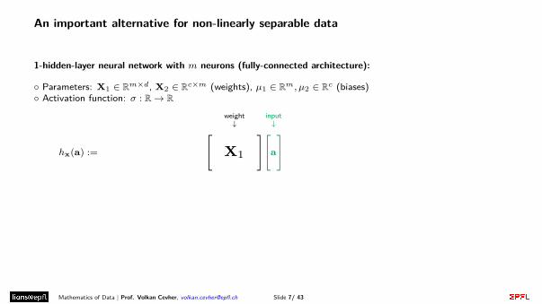
An important alternative for non-linearly separable data
1-hidden-layer neural network with m neurons (fully-connected architecture):
◦ Parameters: X1 ∈ Rm×d, X2 ∈ Rc×m (weights), µ1 ∈ Rm, µ2 ∈ Rc (biases)◦ Activation function: σ : R→ R
hx(a) :=
[X2
]
activationyσ
weight↓[
X1
]
input↓[a
]
+
bias↓[µ1
]
︸ ︷︷ ︸
hidden layer = learned features
+
bias↓[µ2
], x := [X1,X2, µ1, µ2]
recursively repeat activation + affine transformation to obtain “deeper” networks.
Mathematics of Data | Prof. Volkan Cevher, [email protected] Slide 7/ 43
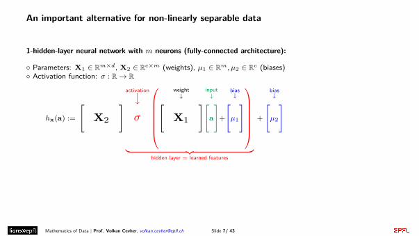
An important alternative for non-linearly separable data
1-hidden-layer neural network with m neurons (fully-connected architecture):
◦ Parameters: X1 ∈ Rm×d, X2 ∈ Rc×m (weights), µ1 ∈ Rm, µ2 ∈ Rc (biases)◦ Activation function: σ : R→ R
hx(a) :=
[X2
]
activationyσ
weight↓[
X1
] input↓[a
]
+
bias↓[µ1
]
︸ ︷︷ ︸
hidden layer = learned features
+
bias↓[µ2
], x := [X1,X2, µ1, µ2]
recursively repeat activation + affine transformation to obtain “deeper” networks.
Mathematics of Data | Prof. Volkan Cevher, [email protected] Slide 7/ 43

An important alternative for non-linearly separable data
1-hidden-layer neural network with m neurons (fully-connected architecture):
◦ Parameters: X1 ∈ Rm×d, X2 ∈ Rc×m (weights), µ1 ∈ Rm, µ2 ∈ Rc (biases)◦ Activation function: σ : R→ R
hx(a) :=
[X2
]
activationyσ
weight↓[
X1
] input↓[a
]+
bias↓[µ1
]︸ ︷︷ ︸
hidden layer = learned features
+
bias↓[µ2
], x := [X1,X2, µ1, µ2]
recursively repeat activation + affine transformation to obtain “deeper” networks.
Mathematics of Data | Prof. Volkan Cevher, [email protected] Slide 7/ 43

An important alternative for non-linearly separable data
1-hidden-layer neural network with m neurons (fully-connected architecture):
◦ Parameters: X1 ∈ Rm×d, X2 ∈ Rc×m (weights), µ1 ∈ Rm, µ2 ∈ Rc (biases)◦ Activation function: σ : R→ R
hx(a) :=
[X2
] activationyσ
weight↓[
X1
] input↓[a
]+
bias↓[µ1
]︸ ︷︷ ︸
hidden layer = learned features
+
bias↓[µ2
], x := [X1,X2, µ1, µ2]
recursively repeat activation + affine transformation to obtain “deeper” networks.
Mathematics of Data | Prof. Volkan Cevher, [email protected] Slide 7/ 43
An important alternative for non-linearly separable data
1-hidden-layer neural network with m neurons (fully-connected architecture):
◦ Parameters: X1 ∈ Rm×d, X2 ∈ Rc×m (weights), µ1 ∈ Rm, µ2 ∈ Rc (biases)◦ Activation function: σ : R→ R
hx(a) :=
[X2
] activationyσ
weight↓[
X1
] input↓[a
]+
bias↓[µ1
]︸ ︷︷ ︸
hidden layer = learned features
+
bias↓[µ2
]
, x := [X1,X2, µ1, µ2]
recursively repeat activation + affine transformation to obtain “deeper” networks.
Mathematics of Data | Prof. Volkan Cevher, [email protected] Slide 7/ 43

An important alternative for non-linearly separable data
1-hidden-layer neural network with m neurons (fully-connected architecture):
◦ Parameters: X1 ∈ Rm×d, X2 ∈ Rc×m (weights), µ1 ∈ Rm, µ2 ∈ Rc (biases)◦ Activation function: σ : R→ R
hx(a) :=
[X2
] activationyσ
weight↓[
X1
] input↓[a
]+
bias↓[µ1
]︸ ︷︷ ︸
hidden layer = learned features
+
bias↓[µ2
], x := [X1,X2, µ1, µ2]
recursively repeat activation + affine transformation to obtain “deeper” networks.
Mathematics of Data | Prof. Volkan Cevher, [email protected] Slide 7/ 43

Why neural networks?: An approximation theoretic motivation
Theorem (Universal approximation [3])Let σ(·) be a nonconstant, bounded, and increasingcontinuous function. Let Id = [0, 1]d. The space ofcontinuous functions on Id is denoted by C(Id).
Given ε > 0 and g ∈ C(Id) there exists a 1-hidden-layernetwork h with m neurons such that h is anε-approximation of g, i.e.,
supa∈Id
|g(a)− h(a)| ≤ ε
CaveatThe number of neurons m needed to approximate somefunction g can be arbitrarily large! Figure: networks of increasing width
Mathematics of Data | Prof. Volkan Cevher, [email protected] Slide 8/ 43

Why were NNs not popular before 2010?
I too big to optimize!I did not have enough dataI could not find the optimum via algorithms
1
Mathematics of Data | Prof. Volkan Cevher, [email protected] Slide 9/ 43

Why were NNs not popular before 2010?
I too big to optimize!I did not have enough dataI could not find the optimum via algorithms
1
Mathematics of Data | Prof. Volkan Cevher, [email protected] Slide 9/ 43
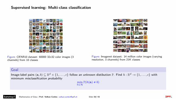
Supervised learning: Multi-class classification
Figure: CIFAR10 dataset: 60000 32x32 color images (3channels) from 10 classes
Figure: Imagenet dataset: 14 million color images (varyingresolution, 3 channels) from 21K classes
GoalImage-label pairs (a, b) ⊆ Rd × {1, . . . , c} follow an unknown distibution P. Find h : Rd → {1, . . . , c} withminimum misclassification probability
minh∈H
P(h(a) , b)
Mathematics of Data | Prof. Volkan Cevher, [email protected] Slide 10/ 43

2010-today: Deep Learning becomes popular again
XRCE (20
11)
AlexNet
(2012
)
ZF (20
13)
VGG (201
4)
Net (20
14)
Human
ResNet
(2015
)
Net-V4 (
2016
)
Classifier
0
5
10
15
20
25
Erro
r rat
e
Linear modelDeep Network
Figure: Error rate on the ImageNet challenge, for different network architectures.
Mathematics of Data | Prof. Volkan Cevher, [email protected] Slide 11/ 43
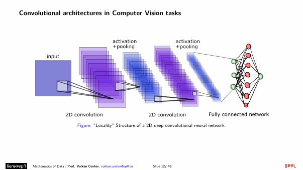
Convolutional architectures in Computer Vision tasks
Figure: “Locality” Structure of a 2D deep convolutional neural network.
Mathematics of Data | Prof. Volkan Cevher, [email protected] Slide 12/ 43

Inductive Bias: Why convolution works so well in Computer Vision tasks?
h◦ true unknown functionH space of all functionsHpfc fully-connected networks
with p parametersHpconv convolutional networks
with p parameters
Mathematics of Data | Prof. Volkan Cevher, [email protected] Slide 13/ 43
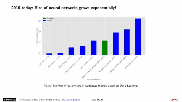
2010-today: Size of neural networks grows exponentially!
ELMo (
AI2 - 2
018)
GPT (O
penA
I - 20
18)
BERT (
- 201
8)
Transf
ormer
ELMo (
AI2 - 2
019)
GPT-2
(OpenA
I - 20
19)
Grover-
Mega (
U. of W
ashing
ton - 2
019)
Megatr
on-LM
(Nvid
ia - 2
019)
Turin
g-NLG
(Micr
osoft -
2020
)
GPT-3
(OpenA
I - 20
20)
Language Model
102
103
104
105
Para
met
ers (
milli
ons)
AcademiaIndustry
Figure: Number of parameters in Language models based on Deep Learning.
Mathematics of Data | Prof. Volkan Cevher, [email protected] Slide 14/ 43

The Landscape of ERM with multilayer networks
Recall: Empirical risk minimization (ERM)Let hx : Rn → R be network and let {(ai, bi)}ni=1 be a sample with bi ∈ {−1, 1} and ai ∈ Rn. The empiricalrisk minimization (ERM) is defined as
minx
{Rn(x) :=
1n
n∑i=1
L(hx(ai), bi)
}(1)
where L(hx(ai), bi) is the loss on the sample (ai, bi) and x are the parameters of the network.
Some frequently used loss functions
I L(hx(a), b) = log(1 + exp(−b · hx(a))) (logistic loss)I L(hx(a), b) = (b− hx(a))2 (squared error)I L(hx(a), b) = max(0, 1− b · hx(a)) (hinge loss)
Mathematics of Data | Prof. Volkan Cevher, [email protected] Slide 15/ 43

The Landscape of ERM with multilayer networks
1
Figure: convex (left) vs non-convex (right) optimization landscape
Conventional wisdom in ML until 2010:Simple models + simple errors
Mathematics of Data | Prof. Volkan Cevher, [email protected] Slide 16/ 43
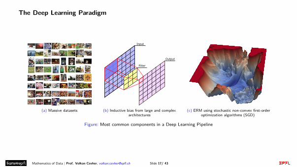
The Deep Learning Paradigm
(a) Massive datasets (b) Inductive bias from large and complexarchitectures
1
(c) ERM using stochastic non-convex first-orderoptimization algorithms (SGD)
Figure: Most common components in a Deep Learning Pipeline
Mathematics of Data | Prof. Volkan Cevher, [email protected] Slide 17/ 43

Challenges in DL/ML applications: Robustness (I)
(a) Turtle classified as rifle. Athalye et al. 2018. (b) Stop sign classified as 45 mph sign. Eykholt et al. 2018
Figure: Natural or human-crafted modifications that trick neural networks used in computer vision tasks
Mathematics of Data | Prof. Volkan Cevher, [email protected] Slide 18/ 43

Challenges in DL/ML applications: Robustness (II)
(a) Linear classifier on data distributed on a sphere (b) Concentration of measure phenomenon on highdimensions
Figure: Understanding the robustness of a classifier in high-dimensional spaces. Shafahi et al. 2019.
Mathematics of Data | Prof. Volkan Cevher, [email protected] Slide 19/ 43

Challenges in DL/ML applications: Robustness (References)
1. Madry, Aleksander and Makelov, Aleksandar and Schmidt, Ludwig and Tsipras, Dimitris and Vladu, Adrian.Towards Deep Learning Models Resistant to Adversarial Attacks. ICLR 2018.
2. Raghunathan, A., Steinhardt, J., and Liang, P. S. Semidefinite relaxations for certifying robustness toadversarial examples. Neurips 2018.
3. Wong, E. and Kolter, Z. (2018). Provable defenses against adversarial examples via the convex outeradversarial polytope. ICML 2018.
4. Huang, X., Kwiatkowska, M., Wang, S., and Wu, M. Safety verification of deep neural networks. ComputerAided Verification 2017.
5. Athalye, A., et al. Synthesizing robust adversarial examples. International conference on machine learning.PMLR, 2018.
6. Eykholt, K., Evtimov, I., Fernandes, E., Li, B., Rahmati, A., Xiao, C., and Song, D. Robust physical-worldattacks on deep learning visual classification. In Proceedings of the IEEE Conference on Computer Visionand Pattern Recognition (pp. 1625-1634). 2018.
7. Shafahi A., Ronny Huang, W., Studer, C., Feizi, S. and Goldstein, T. Are adversarial examples inevitable?.International Conference on Learning Representations. 2019.
Mathematics of Data | Prof. Volkan Cevher, [email protected] Slide 20/ 43

Challenges in DL/ML applications: Surveillance/Privacy/Manipulation
Figure: Political and societal concerns about some DL/ML applications
Mathematics of Data | Prof. Volkan Cevher, [email protected] Slide 21/ 43

Challenges in DL/ML applications: Surveillance/Privacy/Manipulation (References)
1. Dwork, C., and Roth, A. The Algorithmic Foundations of Differential Privacy. Foundations and Trends inTheoretical Computer Science, 9, 2013.
2. Abadi, M., Chu, A., Goodfellow, I., McMahan, H. B., Mironov, I., Talwar, K., and Zhang, L. Deep learningwith differential privacy. In Proceedings of the 2016 ACM SIGSAC Conference on Computer andCommunications Security (pp. 308-318). 2016.
3. Sreenu, G., Saleem Durai, M.A. Intelligent video surveillance: a review through deep learning techniques forcrowd analysis. J Big Data 6, 48. 2019.
4. O’Neil, C., Weapons of Math Destruction: How Big Data Increases Inequality and Threatens DemocracyBroadway Books, (2016);
5. Wade, M. Psychographics: the behavioural analysis that helped Cambridge Analytica know voters’ minds.https://theconversation.com/psychographics-the-behavioural-analysis-that-helped-cambridge-analytica-know-voters-minds-93675 2018.
Mathematics of Data | Prof. Volkan Cevher, [email protected] Slide 22/ 43

Challenges in DL/ML applications: Fairness
4ML & AI | Volkan Cevher | https://lions.epfl.ch (a) Racist classifier
5ML & AI | Volkan Cevher | https://lions.epfl.ch (b) Effect of unbalanced data
Figure: Unfair classifiers due to biased or unbalanced datasets/algorithms
Mathematics of Data | Prof. Volkan Cevher, [email protected] Slide 23/ 43

Challenges in DL/ML applications: Fairness (References)
1. Barocas, S. Hardt, M. Narayanan, Arvind. Fairness in Machine Learning Limitations and Opportunities.https://fairmlbook.org/pdf/fairmlbook.pdf 2020.
2. Hardt, M. How Big Data Is Unfair.https://medium.com/@mrtz/how-big-data-is-unfair-9aa544d739de 2014.
3. Munoz, C., Smith, M., and Patil, D. Big Data: A Report on Algorithmic Systems, Opportunity, and CivilRights. Executive Office of the President. The White House, 2016.
4. Campolo, A., Sanfilippo, M., Whittaker, M., Crawford, K. AI Now 2017 Report. AI Now Institute at NewYork University, 2017.
5. Friedman, B. and Nissenbaum, H. Bias in Computer Systems. ACM Transactions on Information Systems(TOIS) 14, no. 3. 1996: 330–47.
6. Pedreshi, D., Ruggieri, S. and Turini, F. Discrimination-Aware Data Mining. Proc. 14th SIGKDD. ACM2008.
7. Noble, S.U. Algorithms of Oppression: How Search Engines Reinforce Racism. NYU Press. 2018.
Mathematics of Data | Prof. Volkan Cevher, [email protected] Slide 24/ 43

Challenges in DL/ML applications: InterpretabilityInterpretability
3ML & AI | Volkan Cevher | https://lions.epfl.ch Figure: Performance vs Interpretability trade-offs in DL/ML
Mathematics of Data | Prof. Volkan Cevher, [email protected] Slide 25/ 43

Challenges in DL/ML applications: Interpretability (References)
1. Baehrens, David and Schroeter, Timon and Harmeling, Stefan and Kawanabe, Motoaki and Hansen, Katjaand Mueller, Klaus-Robert. Simonyan, Karen and Vedaldi, Andrea and Zisserman, Andrew. How to ExplainIndividual Classification Decisions. JMLR 2010.
2. Deep Inside Convolutional Networks: Visualising Image Classification Models and Saliency Maps. arXive-prints. arXiv:1312.6034. 2013.
3. Ribeiro, Marco and Singh, Sameer and Guestrin, Carlos. “Why Should I Trust You?”: Explaining thePredictions of Any Classifier. KDD 2016.
4. Sundararajan, Mukund and Taly, Ankur and Yan, Qiqi. Axiomatic Attribution for Deep Networks. ICML2017.
5. Shrikumar, Avanti and Greenside, Peyton and Kundaje, Anshul. Learning Important Features ThroughPropagating Activation Differences. ICML 2017.
Mathematics of Data | Prof. Volkan Cevher, [email protected] Slide 26/ 43

Challenges in DL/ML applications: Energy efficiency and costSustainability:
Dennard scaling & Moore’s law vs Growth of data
6ML & AI | Volkan Cevher | https://lions.epfl.ch
Andy Burg
Tim Dettmers
DART Consulting
Figure: Efficiency and Scalability concerns in DL/ML
Mathematics of Data | Prof. Volkan Cevher, [email protected] Slide 27/ 43

Challenges in DL/ML applications: Energy efficiency and cost (References)
1. García-Marín, E., Rodrigues, C. F., Riley, G., and Grahn, H. Estimation of energy consumption in machinelearning. Journal of Parallel and Distributed Computing, 134, 75-88. 2019.
2. Strubell, E., Ganesh, A., and McCallum, A. Energy and policy considerations for deep learning in NLP.arXiv preprint arXiv:1906.02243. 2019.
3. Goel, A., Tung, C., Lu, Y. H., and Thiruvathukal, G. K. A Survey of Methods for Low-Power DeepLearning and Computer Vision. arXiv preprint arXiv:2003.11066. 2020.
4. Conti, F., Rusci, M., and Benini, L. The Memory Challenge in Ultra-Low Power Deep Learning. InNANO-CHIPS 2030 (pp. 323-349). Springer, Cham. 2020.
Mathematics of Data | Prof. Volkan Cevher, [email protected] Slide 28/ 43

What theoretical challenges in Deep Learning will we study?
ModelsLet X ⊆ X ◦ be parameter domains, where X is known. Define1. x◦ ∈ arg minx∈X◦ R(x): true minimum risk model2. x\ ∈ arg minx∈X R(x): assumed minimum risk model3. x? ∈ arg minx∈X Rn(x): ERM solution4. xt: numerical approximation of x? at time t
Practical performance in Deep Learning
R(xt)−R(x◦)︸ ︷︷ ︸ε̄(t,n)
≤ Rn(xt)−Rn(x?)︸ ︷︷ ︸optimization error
+2 supx∈X|R(x)−Rn(x)|︸ ︷︷ ︸
worst-case generalization error
+ R(x\)−R(x◦)︸ ︷︷ ︸model error
where ε̄(t, n) denotes the total error of the Learning Machine. In Deep Learning applications1. Optimization error is almost zero, in spite of non-convexity. ⇒ lecture 92. We expect large generalization error. It does not happen in practice. ⇒ lecture 7 (this one) and 83. Large architectures + inductive bias might lead to small model error.
Mathematics of Data | Prof. Volkan Cevher, [email protected] Slide 29/ 43

Generalization error bounds
The value of |R(x)−Rn(x)| is called the generalization error of the parameter x.
Goal: obtain generalization bounds for multi-layer, fully-connected neural networks
We want to find high-probability upper bounds for the worst case generalization error over a class X :
supx∈X|R(x)−Rn(x)|
Main tool: concentration inequalities!I Measure of how far is an empirical average from the true mean
Theorem (Hoeffding’s Inequality [6])Let Y1, . . . , Yn be i.i.d. random variables with Yi taking values in the interval [ai, bi] ⊆ R for all i = 1, . . . , n.Let Sn := 1
n
∑n
i=1 Yi. It holds that
P (|Sn − E[Sn]| > t) ≤ 2 exp(−
2n2t2∑n
i=1(bi − ai)2
)
Mathematics of Data | Prof. Volkan Cevher, [email protected] Slide 30/ 43

Warmup: Generalization bound for a singleton
LemmaFor i = 1, . . . , n let (ai, bi) ∈ Rp × {−1, 1} be independent random variables and hx : Rp → R be a functionparametrized by x ∈ X . Let X = {x0} and L(hx(a), b) = {sign(hx(a)) , b} be the 0-1 loss.With probability at least 1− δ, we have that
supx∈X|R(x)−Rn(x)| = |R(x0)−Rn(x0)| ≤
√ln(2/δ)
2n.
Proof.Note that E[ 1
n
∑n
i=1 L(hx0 (ai), bi)] = R(x0), the expected risk of the parameter x0. MoreoverL(hx0 (ai), bi) ∈ [0, 1]. We can use Hoeffding’s inequality and obtain
P(|Rn(x0)−R(x0)| > t) = P
(∣∣∣∣∣ 1n
n∑i=1
Li(hx0 (ai), bi)−R(x0)
∣∣∣∣∣ > t
)≤ 2 exp
(− 2nt2
)Setting δ := 2 exp
(−2nt2
), we have that t =
√ln 2/δ
2n , thus obtaining the result.�
Mathematics of Data | Prof. Volkan Cevher, [email protected] Slide 31/ 43

Generalization bound for finite sets
LemmaFor i = 1, . . . , n let (ai, bi) ∈ Rp × {−1, 1} be independent random variables and hx : Rp → R be a functionparametrized by x ∈ X . Let X be a finite set and L(hx(a), b) = {sign(hx(a)) , b} be the 0-1 loss.With probability at least 1− δ, we have that
supx∈X|R(x)−Rn(x)| ≤
√ln |X |+ ln(2/δ)
2n.
Proof.Let X = {x1, . . . ,x|X|}. We can use a union bound and the analysis of the singleton case to obtain:
P(∃j : |Rn(xj)−R(xj)| > t) ≤|X|∑j=1
P(|Rn(xj)−R(xj)| > t) = 2|X | exp(− 2nt2
)
Setting δ := 2|X | exp(−2nt2
)we have that t =
√ln |X|+ln 2
δ2n , thus obtaining the result.
�
Mathematics of Data | Prof. Volkan Cevher, [email protected] Slide 32/ 43

Generalization bounds for infinite classes - The Rademacher complexity
However, in most applications in ML/DL we optimize over an infinite parameter space X !
◦ A useful notion of complexity to derive generalization bounds for infinite classes of functions:
Definition (Rademacher Complexity [2])Let S = {a1, . . . ,an} ⊆ Rp and let {σi : i = 1, . . . , n} be independent Rademacher random variables i.e.,taking values uniformly in {−1,+1} (coin flip). Let H be a class of functions of the form h : Rp → R. TheRademacher complexity of H with respect to A is defined as follows:
RA(H) B E suph∈H
1n
n∑i=1
σih(ai).
◦ RA(H) measures how well can we fit random signs (±1) with the output of an element of H on the set A.
Mathematics of Data | Prof. Volkan Cevher, [email protected] Slide 33/ 43

Visualizing Rademacher complexity
Figure: Rademacher complexity measures correlation with random signs
Mathematics of Data | Prof. Volkan Cevher, [email protected] Slide 34/ 43

Visualizing Rademacher complexity
(a) High Rademacher Complexity (b) Large Generalization error(memorization)
(c) Low Rademacher Complexity (d) Low Generalization error
Figure: Rademacher complexity and Generalization error
Mathematics of Data | Prof. Volkan Cevher, [email protected] Slide 35/ 43

A fundamental theorem about the Rademacher Complexity
Theorem (See Theorem 3.3 and 5.8 in [6])Suppose that the loss function has the form L(hx(a), b) = φ(b · hx(a)) for a 1-Lipschitz function φ : R→ R.
Let HX := {hx : x ∈ X} be a class of parametric functions hx : Rp → R. For any δ > 0, with probability atleast 1− δ over the draw of an i.i.d. sample {(ai, bi)}ni=1, letting A = (a1, . . . ,an), the following holds:
supx∈X|Rn(x)−R(x)| ≤ 2EARA(HX ) +
√ln(2/δ)
2n,
supx∈X|Rn(x)−R(x)| ≤ 2RA(HX ) + 3
√ln(4/δ)
2n.
The assumption is satisfied for common losses
I L(hx(a), b) = log(1 + exp(−b · hx(a)))⇒ φ(z) := log(1 + exp(z)) (logistic loss)I L(hx(a), b) = max(0, 1− b · hx(a))⇒ φ(z) := max(0, 1− z) (hinge loss)
Mathematics of Data | Prof. Volkan Cevher, [email protected] Slide 36/ 43

Computing the Rademacher complexity for Linear functions
TheoremLet X := {x ∈ Rp : ‖x‖2 ≤ λ} and let HX be the class of functions of the form hx : Rp → R, hx(a) = 〈x,a〉,for some x ∈ X}. Let A = {a1, . . . ,an} ⊆ Rp such that maxi=1,...,n ‖ai‖ ≤M . It holds thatRA(HX ) ≤ λM/
√n.
Proof.
RA(HX ) = E sup‖x‖2≤λ
1n
n∑i=1
σi〈x,a〉
= E sup‖x‖2≤λ
1n
⟨x,
n∑i=1
σia
⟩
≤1nλE
∥∥∥∥∥n∑i=1
σiai
∥∥∥∥∥2
(C-S)
⇒RA(HX ) ≤1nλ
(E
n∑i=1
‖σiai‖22
)1/2
(Jensen)
≤1nλ
(n∑i=1
‖ai‖22
)1/2
≤ λM/√n
�
Mathematics of Data | Prof. Volkan Cevher, [email protected] Slide 37/ 43

Rademacher complexity estimates of fully connected Neural Networks
NotationFor a matrix X ∈ Rn,m, ‖X‖ denotes its spectral norm. Let X:,k be the k-th column of X. We define
‖X‖2,1 = ‖(‖X:,1‖2, . . . , ‖X:,m‖2)‖1. (2)
Theorem (Spectral bound [1])For positive integers p0, p1, . . . , pd = 1, and positive reals λ1, . . . , λd ν1, . . . , νd define the set
X := {(X1, . . . ,Xd) : Xi ∈ Rpi×pi−1 , ‖Xi‖ ≤ λi, ‖XTi ‖2,1 ≤ νi}.
Let HX be the class of neural networks hx : Rp → R, hx = Xd ◦ σ ◦ . . . ◦ σ ◦X1 where x = (X1, . . . ,Xd) ∈ X .Suppose that σ is 1-Lipschitz. Let A = {a1, . . . ,an} ⊆ Rp, M := maxi=1,...,n ‖ai‖ andW := max{pi : i = 0, . . . , d}.
The Rademacher complexity of HX with respect to A is bounded as
RA(HX ) = O
log(W )M√n
d∏i=1
λi
(d∑j=1
ν2/3j
λ2/3j
)3/2 (3)
Mathematics of Data | Prof. Volkan Cevher, [email protected] Slide 38/ 43

How well do complexity measures correlate with generalization?
name definition correlation1
Frobenius distance to initialization [7]∑d
i=1 ‖Xi −X0i ‖
2F −0.263
Spectral complexity2 [1]∏d
i=1 ‖Xi‖(∑d
i=1‖Xi‖
3/22,1
‖Xi‖3/2
)2/3
−0.537
Parameter Frobenius norm∑d
i=1 ‖Xi‖2F 0.073Fisher-Rao [5] (d+1)2
n
∑n
i=1 〈x,∇x`(hx(ai), bi)〉 0.078Path-norm [8]
∑(i0,...,id)
∏d
j=1
(Xij ,ij−1
)20.373
Table: Complexity measures compared in the empirical study [4], and their correlation with generalization
Complexity measures are still far from explaining generalization in Deep Learning!
1Kendall’s rank correlation coefficient.2The definition in [4] differs slightly.
Mathematics of Data | Prof. Volkan Cevher, [email protected] Slide 39/ 43

Wrap up!
◦ Deep learning recitation on Friday!
Mathematics of Data | Prof. Volkan Cevher, [email protected] Slide 40/ 43
References I
[1] Peter L Bartlett, Dylan J Foster, and Matus J Telgarsky.Spectrally-normalized margin bounds for neural networks.In I. Guyon, U. V. Luxburg, S. Bengio, H. Wallach, R. Fergus, S. Vishwanathan, and R. Garnett, editors,Advances in Neural Information Processing Systems 30, pages 6240–6249. Curran Associates, Inc., 2017.
[2] Peter L Bartlett and Shahar Mendelson.Rademacher and gaussian complexities: Risk bounds and structural results.Journal of Machine Learning Research, 3(Nov):463–482, 2002.
[3] George Cybenko.Approximation by superpositions of a sigmoidal function.Mathematics of control, signals and systems, 2(4):303–314, 1989.
[4] Yiding Jiang*, Behnam Neyshabur*, Hossein Mobahi, Dilip Krishnan, and Samy Bengio.Fantastic generalization measures and where to find them.In International Conference on Learning Representations, 2020.
[5] Tengyuan Liang, Tomaso Poggio, Alexander Rakhlin, and James Stokes.Fisher-rao metric, geometry, and complexity of neural networks.volume 89 of Proceedings of Machine Learning Research, pages 888–896. PMLR, 16–18 Apr 2019.
Mathematics of Data | Prof. Volkan Cevher, [email protected] Slide 41/ 43

References II
[6] Mehryar Mohri, Afshin Rostamizadeh, and Ameet Talwalkar.Foundations of Machine Learning.The MIT Press, 2nd edition, 2018.
[7] Vaishnavh Nagarajan and J. Zico Kolter.Generalization in Deep Networks: The Role of Distance from Initialization.arXiv e-prints, page arXiv:1901.01672, January 2019.
[8] Behnam Neyshabur, Ryota Tomioka, and Nathan Srebro.Norm-based capacity control in neural networks.In Conference on Learning Theory, pages 1376–1401, 2015.
Mathematics of Data | Prof. Volkan Cevher, [email protected] Slide 42/ 43


![pascal.frossard@epfl.ch arXiv:1610.08401v1 [cs.CV] 26 … · Universal adversarial perturbations Seyed-Mohsen Moosavi-Dezfooli y seyed.moosavi@epfl.ch Alhussein Fawzi alhussein.fawzi@epfl.ch](https://static.fdocuments.us/doc/165x107/5aeb0a947f8b9a36698dd145/epflch-arxiv161008401v1-cscv-26-adversarial-perturbations-seyed-mohsen.jpg)