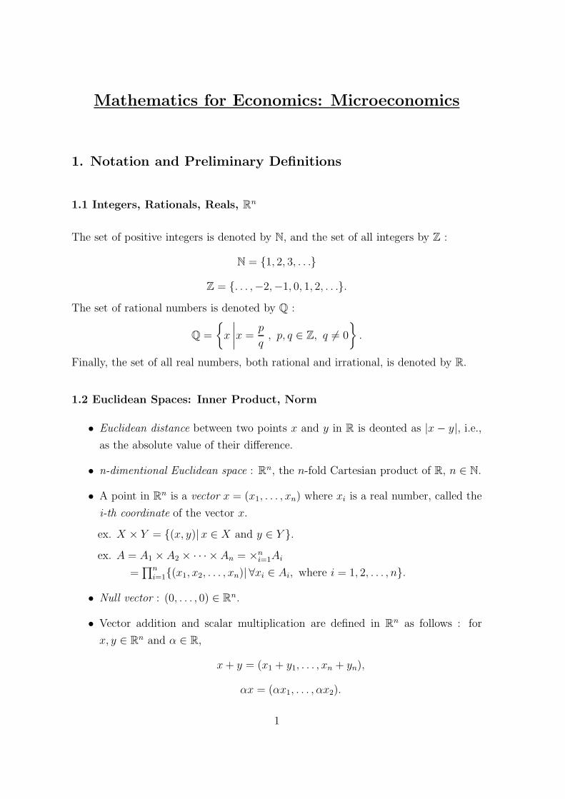
Mathematics for Economics: Microeconomics

1. Notation and Preliminary Definitions

1.1 Integers, Rationals, Reals, Rn

The set of positive integers is denoted by N, and the set of all integers by Z :

N = {1, 2, 3, . . .}

Z = {. . . ,−2,−1, 0, 1, 2, . . .}.

The set of rational numbers is denoted by Q :

Q =

{

x

∣

∣

∣

∣

x =p

q, p, q ∈ Z, q 6= 0

}

.

Finally, the set of all real numbers, both rational and irrational, is denoted by R.

1.2 Euclidean Spaces: Inner Product, Norm

• Euclidean distance between two points x and y in R is deonted as |x − y|, i.e.,

as the absolute value of their difference.

• n-dimentional Euclidean space : Rn, the n-fold Cartesian product of R, n ∈ N.

• A point in Rn is a vector x = (x1, . . . , xn) where xi is a real number, called the

i-th coordinate of the vector x.

ex. X × Y = {(x, y)| x ∈ X and y ∈ Y }.

ex. A = A1 × A2 × · · · × An = ×ni=1Ai

=∏n

i=1{(x1, x2, . . . , xn)| ∀xi ∈ Ai, where i = 1, 2, . . . , n}.

• Null vector : (0, . . . , 0) ∈ Rn.

• Vector addition and scalar multiplication are defined in Rn as follows : for

x, y ∈ Rn and α ∈ R,

x + y = (x1 + y1, . . . , xn + yn),

αx = (αx1, . . . , αx2).

1

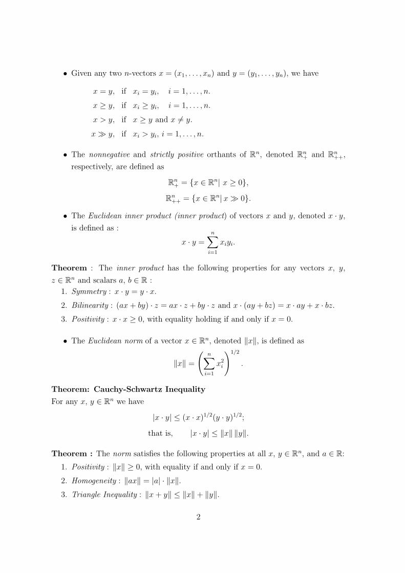
• Given any two n-vectors x = (x1, . . . , xn) and y = (y1, . . . , yn), we have

x = y, if xi = yi, i = 1, . . . , n.

x ≥ y, if xi ≥ yi, i = 1, . . . , n.

x > y, if x ≥ y and x 6= y.

x � y, if xi > yi, i = 1, . . . , n.

• The nonnegative and strictly positive orthants of Rn, denoted Rn+ and Rn

++,

respectively, are defined as

Rn+ = {x ∈ Rn| x ≥ 0},

Rn++ = {x ∈ Rn| x � 0}.

• The Euclidean inner product (inner product) of vectors x and y, denoted x · y,

is defined as :

x · y =

n∑

i=1

xiyi.

Theorem : The inner product has the following properties for any vectors x, y,

z ∈ Rn and scalars a, b ∈ R :

1. Symmetry : x · y = y · x.

2. Bilinearity : (ax + by) · z = ax · z + by · z and x · (ay + bz) = x · ay + x · bz.

3. Positivity : x · x ≥ 0, with equality holding if and only if x = 0.

• The Euclidean norm of a vector x ∈ Rn, denoted ‖x‖, is defined as

‖x‖ =

(

n∑

i=1

x2i

)1/2

.

Theorem: Cauchy-Schwartz Inequality

For any x, y ∈ Rn we have

|x · y| ≤ (x · x)1/2(y · y)1/2;

that is, |x · y| ≤ ‖x‖ ‖y‖.

Theorem : The norm satisfies the following properties at all x, y ∈ Rn, and a ∈ R:

1. Positivity : ‖x‖ ≥ 0, with equality if and only if x = 0.

2. Homogeneity : ‖ax‖ = |a| · ‖x‖.

3. Triangle Inequality : ‖x + y‖ ≤ ‖x‖ + ‖y‖.

2

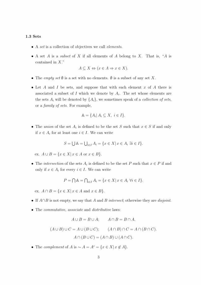
1.3 Sets

• A set is a collection of objectives we call elements.

• A set A is a subset of X if all elements of A belong to X. That is, “A is

contained in X.”

A ⊆ X ⇔ (x ∈ A ⇒ x ∈ X).

• The empty set ∅ is a set with no elements. ∅ is a subset of any set X.

• Let A and I be sets, and suppose that with each element x of A there is

associated a subset of I which we denote by Ai. The set whose elements are

the sets Ai will be denoted by {Ai}, we sometimes speak of a collection of sets,

or a family of sets. For example,

A = {Ai|Ai ⊆ X, i ∈ I}.

• The union of the set Ai is defined to be the set S such that x ∈ S if and only

if x ∈ Ai for at least one i ∈ I. We can write

S =⋃

A =⋃

i∈I Ai = {x ∈ X| x ∈ Ai ∃i ∈ I}.

ex. A ∪ B = {x ∈ X| x ∈ A or x ∈ B}.

• The intersection of the sets Ai is defined to be the set P such that x ∈ P if and

only if x ∈ Ai for every i ∈ I. We can write

P =⋂

A =⋂

i∈I Ai = {x ∈ X| x ∈ Ai ∀i ∈ I}.

ex. A ∩ B = {x ∈ X| x ∈ A and x ∈ B}.

• If A∩B is not empty, we say that A and B intersect; otherwise they are disjoint.

• The commutative, associate and distributive laws:

A ∪ B = B ∪ A; A ∩ B = B ∩ A.

(A ∪ B) ∪ C = A ∪ (B ∪ C); (A ∩ B) ∩ C = A ∩ (B ∩ C).

A ∩ (B ∪ C) = (A ∩ B) ∪ (A ∩ C).

• The complement of A is ∼ A = Ac = {x ∈ X| x 6∈ A}.

3

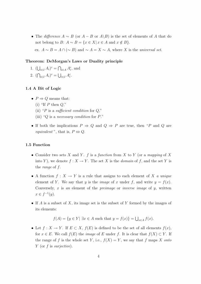
• The difference A ∼ B (or A − B or A\B) is the set of elements of A that do

not belong to B: A ∼ B = {x ∈ X| x ∈ A and x /∈ B}.

ex. A ∼ B = A ∩ (∼ B) and ∼ A = X ∼ A, where X is the universal set.

Theorem: DeMorgan’s Laws or Duality principle

1. (⋃

i∈I Ai)c =

⋂

i∈A Aci , and

2. (⋂

i∈I Ai)c =

⋃

i∈I Aci .

1.4 A Bit of Logic

• P ⇒ Q means that:

(i) “If P then Q,”

(ii) “P is a sufficient condition for Q,”

(iii) “Q is a necessary condition for P .”

• If both the implications P ⇒ Q and Q ⇒ P are true, then “P and Q are

equivalent ”, that is, P ⇔ Q.

1.5 Function

• Consider two sets X and Y . f is a function from X to Y (or a mapping of X

into Y ), we denote f : X → Y . The set X is the domain of f , and the set Y is

the range of f .

• A function f : X → Y is a rule that assigns to each element of X a unique

element of Y . We say that y is the image of x under f , and write y = f(x).

Conversely, x is an element of the preimage or inverse image of y, written

x ∈ f−1(y).

• If A is a subset of X, its image set is the subset of Y formed by the images of

its elements:

f(A) = {y ∈ Y | ∃x ∈ A such that y = f(x)} =⋃

x∈A f(x).

• Let f : X → Y . If E ⊂ X, f(E) is defined to be the set of all elements f(x),

for x ∈ E. We call f(E) the image of E under f . It is clear that f(X) ⊂ Y . If

the range of f is the whole set Y , i.e., f(X) = Y , we say that f maps X onto

Y (or f is surjective).

4

• If E ⊂ Y , f−1(E) denotes the set of all x ∈ X such that f(x) ∈ E. We call

f−1(E) the inverse image of E under f . If y ∈ Y , f−1(y) is the set of all x ∈ X

such that f(x) = y. If for each y ∈ Y , f−1(y) consists of at most one element

of X, then f is said to be a one-to-one mapping of X into Y (or f is injective).

That is, f(x1) 6= f(x2), ∀x1 6= x2, x1, x2 ∈ A, or

∀x1, x2 ∈ X, f(x1) = f(x2) ⇒ x1 = x2.

• If there exists a one-to-one mapping of X onto Y , X and Y can be put in

one-to-one correspondence (or f is bijective). That is, if each element of Y has

an inverse image and that inverse image is unique.

• Given a function f , its inverse relation f−1 : y → x may or may not be a

function (i.e. a correspondence).

• If f : X → Y and g : Y → Z, then their composition, g ◦ f is the function of X

to Z defined by (g ◦ f)(x) = g[f(x)]. By the associative law, we can obtain:

(h ◦ g) ◦ f = h ◦ (g ◦ f) = h ◦ g ◦ f.

2. Basic Topology

2.1 Finite, Countable, and Uncountable Sets

• If there exists a one-to-one mapping of A onto B, A and B can be put in one-

to-one correspondence, or A and B have the same cardinal number, or, briefly,

A and B are numerically equivalent, and we write A ∼ B. The relation has the

following propereties:

1. It is reflexive: A ∼ A.

2. It is symmetric: If A ∼ B, then B ∼ A.

3. It is transitive: If A ∼ B and B ∼ C, then A ∼ C.

• For any positive integer n, let Jn be the set whose elements are the integers

1, 2, . . . , n; let J be the set consisting of all positive integers (i.e. J ∈ Z+ =

{1, 2, . . .}). For any set A, we say:

1. A is finite if A ∼ Jn for some n (the empty set is considered to be finite).

2. A is infinite if A is not finite.

3. A is countable if A ∼ J .

5

4. A is uncountable if A is neither finite nor countable.

5. A is at most countable if A is finite or countable.

Theorem: Every subset of a countable set A is countable.

Theorem: The union of countable sets must be a countable set.

Theorem: Let A be a countable set, and let Bn be the set of all n-tuples (a1, . . . , an),

where ak ∈ A(k = 1, . . . , n), and the elements a1, . . . , an need not be distinct. Then

Bn is countable.

Theorem: If a set A is infinite, then A needs not be countable. Alternatively, all

finite sets are countable, but not all countable sets are finite.

2.2 Metric Spaces

• A set X, whose elements we shall call points, is a “metric space” if with any

two points p and q of X there is associated a real number d(p, q), called the

distance from p to q. We can denote a metric space as (X, d).

• Euclidean distance : d(x, y) between two vectors x and y in Rn is given by

d(x, y) =

√

√

√

√

n∑

i=1

(xi − yi)2.

• The distance function d is called a metric, and is related to the norm ‖ · ‖

through the identity

d(x, y) = ‖x − y‖ for all x, y ∈ Rn.

• Given a metric space, we can define the distance between two points, between

a point and a set, or two sets.

d(x, A) = infa∈A

d(x, a) ⇒ between a point and a set;

d(A, B) = infa∈A

d(B, a) = inf{d(a, b)| a ∈ A, b ∈ B} ⇒ between two sets.

Theorem : The metric d satisfies the following properties at all x, y, z ∈ Rn

6

1. Positivity : d(x, y) ≥ 0 with equality if and only if x = y.

2. Symmetry : d(x, y) = d(y, x).

3. Triangle Inequality : d(x, z) ≤ d(x, y) + d(y, z) for all x y, z ∈ Rn.

• By the segment (a, b) we mean the set of all real numbers x such that a < x < b.

• By the interval [a, b] we mean the set of all real numbers x such that a ≤ x ≤ b.

The half-open interval: (a, b] or [a, b).

2.3 Open Balls, Open Sets, Closed Sets

Given a metric space (X, d) and A, B, E ⊂ X.

• If x ∈ Rn and r > 0, the open (or closed) ball B with the center at x and radius

r is defined to be the set of all y ∈ Rn such that ‖y − x‖ < r (or ‖y − x‖ ≤ r).

We can denote Br(x) as follows.

Br(x) = {y ∈ X| d(x, y) < r} ⇒ open ball,

Br[x] = {y ∈ X| d(x, y) ≤ r} ⇒ closed ball.

• A set E ⊂ Rn is convex if λx + (1 − λ)y ∈ E, where x, y ∈ E, and λ ∈ (0, 1).

• All balls are convex.

• A neighborhood of a point x is a set Bε(x) consisting of all points y such that

d(x, y) < ε, where ε → 0.

• A point xc is a limit point of E if any open ball around it contains at least one

point in E. We denote E ′.

xc ∈ E ′ ⇔ ∀ε > 0, Bε(xc) ∩ E 6= ∅

• If x ∈ E and x is not a limit point of E, then x is an isolated point of E.

• E is closed if every limit point of E is a point of E.

7

• A point xi is an interior point of E if there exists an open ball centered at xi,

Bε(xi) that is contained in E, we denote intE.

xi ∈ intE ⇔ ∃ε > 0 such that Bε(xi) ⊆ E

• A point xe is an exterior point of E if there exists some open ball around xe

that is contained in ∼ E or Ec, we denote extE.

xe ∈ extE ⇔ ∃ε > 0 such that Bε(xe) ⊆ Ec

• A point xb is a boundary point of E if any open ball around it intersects both

E and Ec. We denote ∂E.

xb ∈ ∂E ⇔ ∀ε > 0, Bε(xb) ∩ E 6= ∅ and Bε(xb) ∩ Ec 6= ∅

• E is open if every point of E is an interior point of E.

• E is bounded if there is a (finite) real number M and a point y ∈ X such that

d(x, y) < M for all x ∈ E.

• E is dense in X if every point of X is a limit point of E, or a point of E, or

both.

Theorem: An interior point of a set E must be a limit point of E.

Theorem: Every neighborhood is an open set.

Theorem: A set E is open if and only if its complement is closed; and vice versa.

Theorem: Properties of open sets

1. ∅ and X are open in X.

2. For any (possibily infinite) collection {Gi} of open sets,⋃

i Gi is open.

3. For a finite collection G1, . . . , Gn of open sets,⋂n

i=1 Gi is open.

ex. open intervals: (−1, 1), (−1/2, 1/2), . . . , (−1/n, 1/n).

The intersection of the infinite family of open intervals: {0} ⇒ is not open.

Theorem: Properties of closed sets

1. ∅ and X are closed in X.

2. For any (possibily infinite) collection {Fi} of closed sets,⋂

i Fi is closed.

3. For a finite collection F1, . . . , Fn of closed sets,⋃n

i=1 Fi is closed.

ex. closed intervals: [1, 3−1/n], n = 1, . . . ,∞ ⇒⋃∞

i=1[1, 3−1/n] = [1, 3) (not closed).

8

2.4 Bounded Sets and Compact Sets

• If X is a metric space, E ⊂ X, and if E ′ denotes the set of all limit points of E

in X, then the closure of E is the set E = E ∪ E ′. Intuitively, the closure of E

is the “smallest” closed set that contains E. Note that E = E if and only if E

is itself closed.

• By an open cover of a set E in a metric space X we mean a collection {Gi} of

open subsets of X such that E ⊂⋃

i Gi.

• A subset K of a metric space X is compact if every open cover of K contains a

finite subcover.

Theorem:

1. intE is the largest open set contained in E.

2. E is open if and only if E =intE.

3. E is the smallest closed set that contains E.

4. E is closed if and only if E = E.

Theorem: Suppose K ⊂ Y ⊂ X. Then K is compact relative to X if and only if K

is compact relative to Y .

Theorem: If a set E in Rn has one of the following three properties, then it has the

other two:

1. E is closed and bounded.

2. E is compact.

3. Every infinite subset of E has a limit point in E.

3. Sequences

3.1 Sequences and Limits

• A sequence in Rm is the specification of a point xn ∈ Rm for each integer

n ∈ {1, 2, . . .}. The sequence {xn} is written as x1, x2, x3, . . . .

9

• A sequence of points {xn} converges to a limit x (wirtten xn → x or limn→∞ xn =

x) if the distance d(xn, x) between xn and x tends to zero as n goes to infinity,

i.e., if for all ε > 0, there exists an integer N(ε) such that for all n ≥ N(ε), we

have d(xn, x) < ε. The sequence {xn} is called a convergent sequence.

∀ε > 0, ∃N(ε) such that n > N(ε) ⇒ d(xn, x) < ε [or xn ∈ Bε(x)]

Theorem: A convergent sequence can have at most one limit.

Theorem : Every convergent sequence in Rm is bounded.

Theorem : A sequence {xk} in Rm converges to a limit x if and only if xki → xi for

each i ∈ {1, . . . , m}, where xk = (xk1, . . . , x

km) and x = (x1, . . . , xm).

Theorem : Let {xk} be a sequence in Rm converging to a limit x. Suppose that for

every k, we have a ≤ xk ≤ b, where a = (a1, . . . , am) and b = (b1, . . . , bm) are some

fixed vectors in Rm. Then, it is also the case that a ≤ x ≤ b.

Theorem : Let {xn} and {yn} be convergent real sequences, with {xn} → x and

{yn} → y. If xn ≤ yn for all n, then x ≤ y.

Theorem : Let {xn} and {yn} be convergent real sequences, with {xn} → x and

{yn} → y. Then

(i) {xn + yn} → x + y;

(ii) {xnyn} → xy;

(iii) {xn/yn} → x/y provided y 6= 0 and yn 6= 0 for all n.

3.2 Subsequences

• Let nk be any rule that assigns to each k ∈ N a value nk ∈ N. Suppose that

nk is increasing, i.e., nk < nk+1. Given a sequence {xn} in Rm, we can define

a new sequence {xnk}, whose k-th element is the nk-th element of the sequence

{xn}. The new sequence is called a subsequence of {xn}.

ex. sequence: {0, 1, 0, 1, . . .} ⇒ subsequences: {0, 0, 0, . . .}, {1, 1, 1, . . .}.

• c is a cluster point of {xn} if any open ball with center at c contains infinitely

many terms of the sequence. That is,

∀ε > 0 and ∀N, ∃n > N such that xn ∈ Bε(c)

10

ex. xn = 0 for n even; and xn = 1 for n odd.

⇒ has two cluster points but no limit (does not converge).

• Even if a sequence {xn} is not convergent, it may contain subsequences that

converge.

ex. {0, 1, 0, 1, . . .} ⇒ no limit; but subsequences: {0, 0, 0, . . .} and {1, 1, 1, . . .}

are convergent.

Theorem: Let {xn} be a sequence in a metric space (X, d). If c is a cluster point of

{xn}, then there exists some subsequence {xnk} of {xn} with limit c (i.e. {xnk

} → c).

• If a sequence {xn} is convergent, then every subsequence of {xn} must converge

to x.

• A sequence may have any number of cluster points.

• If a sequence {xn} has no cluster point, then {xn} is a divergent sequence.

3.3 Cauchy Sequences

• A sequence {xn} in Rm is said to satisfy the Cauchy criterion if for all ε > 0,

there is an integer N(ε) such that for all k, l ≥ N(ε), we have d(xk, xl) < ε. A

sequence which satisfies the Cauchy criterion is called a Cauchy sequence.

Theorem: A sequence {xn} in Rm is a Cauchy sequence if and only if it is a conver-

gent sequence, i.e., if and only if there is a x ∈ Rm such that xn → x.

Theorem: Let {xn} be a Cauchy sequence in Rm. Then

1. {xn} is bounded.

2. {xn} has at most one cluster point.

3.4 Suprema, Infima, Maxima, Minima

• α is the least upper bound of X or the supremum of X (denoted by sup X).

That is,

α = {x ∈ R| x ≥ y, ∀y ∈ X and if z ≥ y, ∀y ∈ X, then z ≥ x}.

11

• α is the greatest lower bound of X or the infimum of X (denoted by inf X).

That is,

α = {x ∈ R| x ≤ y, ∀y ∈ X and if z ≤ y, ∀y ∈ X, then z ≤ x}.

• Suppose X ⊂ R. m is a maximum in X, that is, m = {x ∈ X| x ≥ y, ∀y ∈ X}.

We denote the maximum of X as max X.

• Suppose X ⊂ R. m is a minimum in X, that is, m = {x ∈ X| x ≤ y, ∀y ∈ X}.

We denote the minimum of X as min X.

• X ⊂ R, if there is a M ∈ R such that x ≤ M , ∀x ∈ X, then we call X is

bounded above.

• X ⊂ R, if there is a M ∈ R such that x ≥ M , ∀x ∈ X, then we call X is

bounded below.

Theorem: If X is bounded above and closed, then sup X ∈ X. That is, the max X

exists. Similarly, if X is bounded below and closed, then inf X ∈ X. That is, the

min X exists.

Theorem: The supremum property

Every nonempty set of real numbers that is bounded above has a supremum. This

supremum is a real number.

Theorem: The infimum property

Every nonempty set of real numbers that is bounded below has an infimum. This

supremum is a real number.

Axiom of completeness: Let L and H be nonempty sets of real numbers, with the

property that

∀l ∈ L and ∀h ∈ H, l ≤ h.

Then there exists a real number α such that

∀l ∈ L and ∀h ∈ H, l ≤ α ≤ h.

Theorem: The supremum/infimum property implies the axiom of completeness.

12

3.5 Monotone Sequences

• A sequence {xk} in R is a monotone increasing sequence if xk+1 ≥ xk for all k.

It is monotone decreasing if xk+1 ≤ xk.

Theorem: Let {xk} be a monotone increasing (decreasing) sequence in R. If {xk}

is unbounded, it must diverge to +∞(−∞). If {xk} is bounded, it must converge to

x, where x is the supremum(infimum) of the set of points {x1, x2, . . .}.

3.6 The Lim Sup and Lim Inf

• The lim sup of the sequence {xk} is defined as k → ∞ of {ak}, where ak =

sup{xk, xk+1, xk+2, . . .}, abbreviated as limk→∞ supl≥k xl, or lim supk→∞ xk.

• The lim inf of the sequence {xk} is defined as k → ∞ of {bk}, where bk =

inf{xk, xk+1, xk+2, . . .}, abbreviated as limk→∞ inf l≥k xl, or lim infk→∞ xk.

Theorem: Let {xk} be a real-valued sequence, and let A denote the set of all cluster

points of {xk} (including ±∞ if {xk} contains such divergent subsequences). Let

a = lim supk→∞ xk and b = lim infk→∞ xk. Then:

1. there exist subsequences m(k) and l(k) of k such that xm(k) → a and xl(k) → b;

2. a = sup A and b = inf A.

Theorem: A sequence {xk} in R converges to a limit x ∈ R if and only if lim supk→∞ xk =

lim infk→∞ xk = x. Equivalently, {xk} converges to x if and only if every subsequence

of {xk} converges to x.

4. Functions

4.1 Continuous Functions

• Let f : S → T , where S ⊂ Rn and T ⊂ Rm. f is continuous at x ∈ S if ∀ε > 0,

there is a δ > 0 such that y ∈ S and d(x, y) < δ implies d(f(x), f(y)) < ε.

⇒ If ∀ε > 0, ∃δ > 0, such that d(x, y) < δ, then d(f(x), f(y)) < ε, ∀x.

That is, if for all sequences {xk} such that xk ∈ S for all k, and limk→∞ xk = x,

then limk→∞ f(xk) = f(x).

13

• A function f : S → T is continuous on S if it is continuous at each point in S.

Theorem: A function f : S ⊂ Rn → Rm is continuous at a point x ∈ S if and only

if for all open sets V ⊂ Rm such that f(x) ∈ V , there is an open set U ⊂ Rn such

that x ∈ U , and f(z) ∈ V for all z ∈ U ∩ S.

Corollary: If S is an open set in Rn, f is continuous on S if and only if f−1(V ) is

an open set in Rn for each open set V in Rm.

Theorem: The properties of continuous functions are as follows:

1. Let f : X → Y , g : X → Y be continuous functions, then f ± g and fg

are continuous functions, too. f(x)/g(x) is continuous at x for all x such that

g(x) 6= 0.

2. f : X → Y , g : Y → Z are continuous functions, then g ◦ f is a continuous

function that g(f(x)) : X → Z.

4.2 Differentiable and Continuously Differentiable Functions

• If Df : S → Rm+n = Rm × Rn is a continuous function, the f is said to be

continuously differentiable on S, and we write f is C1.

• When f is twice-differentiable on S, and for each i, j = 1, . . . , n, the cross-

partial (∂2f/∂xi∂xj) is a continuous function from S to R, we say that f is

twice continuously differentiable on S, and we write f is C2.

Theorem: If f : S → R is a C2 function, D2f is a symmetric matrix, i.e., we have

∂2f

∂xi∂xj(x) =

∂2f

∂xj∂xi(x), for all i, j = 1, . . . , n, and ∀x ∈ S ⊂ Rn.

• An affine function g : Rn → Rm is: g(y) = Ay + b, where A is an m×n matrix,

y is an n-dimensional vector, and b ∈ Rm. When b = 0¯, the function g is called

linear.

• A function f : X ⊆ Rn → R, where X is a cone, is homogeneous of degree k in

X if

f(λx) = λk · f(x), ∀λ > 0.

14

Euler’s Theorem: Let f : X ⊆ Rn → R be a function with continuous partial

derivatives defined on an open cone X. Then f is homogeneous of degree k in X if

and only ifn∑

i=1

fi(x) · xi = k · f(x), ∀x ∈ X.

4.3 Quadratic Forms: Definite and Semidefinite Matrices

• A quadratic form on Rn is a function gA on Rn of the form

gA(x) = x′Ax =

n∑

i=1

n∑

j=1

aijxixj,

where A = (aij) is any symmetric n × n matrix, and x′ = (x1, x2, . . . , xn).

• A quadratic form A is said to be

1. positive definite if we have x′Ax > 0 for all x ∈ Rn, x 6= 0¯.

2. positive semidefinite if we have x′Ax ≥ 0 for all x ∈ Rn, x 6= 0¯.

3. negative definite if we have x′Ax < 0 for all x ∈ Rn, x 6= 0¯.

4. negative semidefinite if we have x′Ax ≤ 0 for all x ∈ Rn, x 6= 0¯.

5. indefinite if it is neither positive nor negative definite, that is, if there exists

vectors x and z ∈ R such that x′Ax < 0 and z′Az > 0.

• Given a quadratic form gA(x) = x′Ax, let λ1, . . . , λn be the eigenvalues of A

(which will be real numbers, because A is symmetric). Then gA(x) is :

1. positive definite ⇔ λi > 0 ∀i = 1, . . . , n.

2. positive semidefinite ⇔ λi ≥ 0 ∀i = 1, . . . , n.

3. negative definite ⇔ λi < 0 ∀i = 1, . . . , n.

4. negative semidefinite ⇔ λi ≤ 0 ∀i = 1, . . . , n.

• Eliminate n−k rows and the corresponding columns of A, we obtain a submatrix

of dimension k×k. The determinant of this submatrix is called a principal minor

of order k of A. We denote it as Aπk .

• The leading principal minors of A: the principal minors obtained by keeping

the first k rows and columns of A. We denote it as Ak.

Ak =

a11 · · · a1k

.... . .

...

ak1 · · · akk

15

• Let an n × n symmetric matrix A be given, and let π = (π1, . . . , πn) be a

permutation of the integers {1, . . . , n}. Denote by Aπ the symmetric n × n

matrix obtained by applying the permutation π to both rows and columns of

A:

Aπ =

aπ1π1. . . aπ1πn

.... . .

...

aπnπ1. . . aπnπn

.

For k ∈ {1, . . . , n}, let Aπk be the n×n symmetric submatrix of Aπ obtained by

retaining only the first k rows and columns:

Aπk =

aπ1π1. . . aπ1πk

.... . .

...

aπkπ1. . . aπkπk

.

• A n × n symmetric matrix A is

1. negative definite⇔ (−1)k|Ak| > 0 ∀k = 1, . . . , n (i.e., sign|Ak| =sign(−1)k);

2. positive definite ⇔ |Ak| > 0 ∀k = 1, . . . , n;

3. negative semidefinite ⇔ (−1)k|Aπk | ≥ 0 ∀k = 1, . . . , n and ∀π ∈ Π;

4. positive semidefinite ⇔ |Aπk | ≥ 0 ∀k = 1, . . . , n and ∀π ∈ Π.

Moreover, a positive(negative) semidefinite quadratic form A is positive(negative)

definite if and only if |A| 6= 0.

• Examples:

(a)

[

1 0

0 1

]

, (b)

[

1 0

0 0

]

, (c)

[

0 1

1 0

]

.

Sol:

(a) is positive definite; (b) is positive semidefinite; (c) is indefinite.

Theorem: Let A be a positive definite n× n matrix. Then, there is γ > 0 such that

if B is any symmetric n× n matrix with |bjk − ajk| < γ for all j, k ∈ {1, . . . , n}, then

B is also positive definite. A similiar statement holds for negative definite matrices

A.

16

4.4 Separation Theorems

• Let p 6= 0¯

be a vector in Rn, and let a ∈ R. The set H defined by H = {x ∈

Rn| p · x = a} is called hyperplane in Rn, and will be denoted H(p, a).

• A hyperplane in R2, for example, is a straight line: H(p, a) = {(x1, x2)| p1x1 +

p2x2 = a}. Similarly, a hyperplane in R3 is a plane.

• Two sets X and Y in Rn are said to be separated by the hyperplane H(p, a) in

Rn if X and Y lies on the opposite sides of H(p, a), i.e., we have

p · x ≤ a, ∀x ∈ X,

p · y ≥ a, ∀y ∈ Y.

Theorem: Let D be a nonempty convex set in Rn, and let x∗ be a point in Rn that

is not in D. Then, there is a hyperplane H(p, a) in Rn with p 6= 0¯

which separates D

and x∗.

Theorem: Let X and Y be convex sets in Rn such that X ∩ Y = ∅. Then, there

exists a hyperplane H(p, a) in Rn which separates X and Y .

4.5 The Intermediate and Mean Value Theorems

Intermediate Value Theorem:

Let D = [a, b] be an interval in R and let f : D → R be a continuous function. If

f(a) < f(b), and if c is a real number such that f(a) < c < f(b), then there exists

x ∈ (a, b) such that f(x) = c. A similar statement holds if f(a) > f(b).

Intermediate Value Theorem for the Derivative:

Let D = [a, b] be an interval in R and let f : D → R be a function that is differentiable

everywhere on D. If f ′(a) < f ′(b), and if c is a real number such that f ′(a) < c < f ′(b),

then there exists a point x ∈ (a, b) such that f ′(x) = c. A similar statement holds if

f ′(a) > f ′(b).

Mean Value Theorem:

Let D = [a, b] be an interval in R and let f : D → R be a continuous function. Suppose

f is differentiable on (a, b). Then, there exists x ∈ (a, b) such that f(b) − f(a) =

(b − a)f ′(x).

17

Taylor’s Theroem:

Let f : D → R be a Cm function, where D is an open interval in R, and m ≥ 0 is a

nonnegative integer. Suppose also that fm+1(z) exists for every point z ∈ D. Then,

for any x, y ∈ D, there is z ∈ (x, y) such that

f(y) =m∑

k=0

(

f (k)(x)(y − x)k

k!

)

+fm+1(z)(y − x)m+1

(m + 1)!.

• When m = 0, Taylor’s theorem reduces to the mean value theorem.

The Intermediate Value Theorem in Rn :

Let D ⊂ Rn be a convex set, and let f : D → R be continuous on D. Suppose

that a and b are points in D such that f(a) < f(b). Then, for any c such that

f(a) < c < f(b), there is a λ ∈ (0, 1) such that f((1 − λ)a + λb) = c.

The Mean Value Theorem in Rn :

Let D ⊂ Rn be open and convex, and let f : S → R be a function that is differentiable

everywhere on D. Then, for any a, b ∈ D, there is a λ ∈ (0, 1) such that

f(b) − f(a) = Df((1 − λ)a + λb) · (b − a).

Taylor’s Theorem in Rn (Taylor Expansion):

Let f : D → R, where D is an open set in Rn. If f is C1 on D, then it is the case

that for any x, y ∈ D, we have

f(y) = f(x) + Df(x)(y − x) + R1(x, y),

where the remainder term R1(x, y) has the property that

limy→x

(

R1(x, y)

‖x − y‖

)

= 0.

If f is C2 on D, this statement can be strengthened to

f(y) = f(x) + Df(x)(y − x) +1

2(y − x)′D2f(x)(y − x) + R2(x, y),

where the remainder term R1(x, y) has the property that

limy→x

(

R2(x, y)

‖x − y‖2

)

= 0.

18

4.6 The Inverse and Implicit Function Theorems

The Inverse Function Theorem:

Let f : S → Rn be a C1 function, where S ⊂ Rn is open. Suppose there is a point

y ∈ S such that the n × n matrix Df(y) is invertible. Let x = f(y). Then

1. There are open sets U and V in Rn such that x ∈ U , y ∈ V , f is one-to-one on

V , and f(V ) = U .

2. The inverse function g : U → V of f is a C1 function on U , whose derivative at

any point x ∈ U satisfies Dg(x) = (Df(y))−1, where g(f(y)) = y or f(y) = x.

The Implicit Function Theorem:

Let F : S ⊂ Rm+n → Rn be a C1 function, where S is open. Let (x∗, y∗) be a

point in S such that DFy(x∗, y∗) is invertible, and let F (x∗, y∗) = c. Then, there is a

neighborhood U ∈ Rm of x∗ and a C1 function g : U → Rn such that

(i) (x, g(x)) ∈ S for all x ∈ U ,

(ii) g(x∗) = y∗,

(iii) F (x, g(x)) ≡ c for all x ∈ U .

The derivative of g at any x ∈ U may be obtained from the chain rule:

Dg(x) = −(DFy(x, y))−1 · DFx(x, y).

5. Correspondences

• Let Θ ⊂ Rm, S ⊂ Rn. A correspondence Φ from Θ to S is a map that associates

with each element θ ∈ Θ a (nonempty) subset Φ(θ) ⊂ S. We will denote a

correspondence Φ from Θ to S by Φ : Θ → P (S), where P (S) denotes the

power set of S, i.e., the set of all nonempty subsets of S.

5.1 Upper- and Lower-Semicontinuous Correspondences

• Any function f from Θ to S may also be viewed as a single-valued correspon-

dence from Θ to S.

• A correspondence Φ : Θ → P (S) is upper-semicontinuous or u.s.c. at a point

θ ∈ Θ if for all open sets V such that Φ(θ) ⊂ V , there exists an open set U

containing θ, such that θ′ ∈ Θ ∩ U implies Φ(θ′) ⊂ V .

19

• A correspondence Ψ : Θ → P (S) is lower-semicontinuous or l.s.c. at θ ∈ Θ if

for all open sets V such that V ∩Ψ(θ) 6= ∅, there exists an open set U containing

θ such that θ′ ∈ Θ ∩ U implies V ∩ Ψ(θ′) 6= ∅.

• The correspondence Φ : Θ → P (S) is continuous at θ ∈ Θ if Φ is both u.s.c.

and l.s.c. at θ.

5.2 Semicontinuous Functions and Semicontinuous Correspondences

Theorem: A single-valued correspondence that is semicontinuous (whether u.s.c. or

l.s.c.) is continuous when viewed as a function. Conversely, every continuous function,

when viewed as a single-valued correspondence, is both u.s.c. and l.s.c..

6. Convexity

6.1 Concave and Convex Functions

• A function f : D → R is concave on D if and only if for all x, y ∈ D and

λ ∈ (0, 1), it is the case that

f [λx + (1 − λ)y] ≥ λf(x) + (1 − λ)f(y).

• A function f : D → R is convex on D if and only if for all x, y ∈ D and

λ ∈ (0, 1), it is the case that

f [λx + (1 − λ)y] ≤ λf(x) + (1 − λ)f(y).

• A function f : D → R is strictly concave on D if for all x, y ∈ D with x 6= y,

and λ ∈ (0, 1), we have

f [λx + (1 − λ)y] > λf(x) + (1 − λ)f(y).

• A function f : D → R is strictly convex on D if for all x, y ∈ D with x 6= y, and

λ ∈ (0, 1), we have

f [λx + (1 − λ)y] < λf(x) + (1 − λ)f(y).

Theorem: A function f : D → R is concave on D if and only if the function −f is

convex on D. It is strictly concave on D if and only if f is strictly convex on D.

20

6.2 Implications of Convexity

Theorem: Let f : D → R be a concave function. Then, if D is open, f is continuous

on D. If D is not open, f is continuous on the interior of D.

Theorem: Let D be an open and convex set in Rn, and let f : D → R be differen-

tiable on D. Then, f is concave on D if and only if

Df(x)(y − x) ≥ f(y) − f(x) for all x, y ∈ D,

while f is convex on D if and only if

Df(x)(y − x) ≤ f(y) − f(x) for all x, y ∈ D.

Theorem: Let f : D → R be a C2 function, where D ⊂ Rn is open and convex.

Then,

1. f is concave on D if and only if D2f(x) is a negative semidefinite matrix for all

x ∈ D.

2. f is convex on D if and only if D2f(x) is a positive semidefinite matrix for all

x ∈ D.

3. If D2f(x) is negative definite for all x ∈ D, then f is strictly concave on D.

4. If D2f(x) is positive definite for all x ∈ D, then f is strictly convex on D.

6.3 Quasi-Concave and Quasi-Convex Functions

• Let D be a convex set in Rn, and f : D → R. The upper-contour set of f at

a ∈ R, denoted Uf(a), is defined as

Uf (a) = {x ∈ D| f(x) ≥ a},

while the lower-contour set of f at a ∈ R, denoted Lf (a), is defined as

Lf (a) = {x ∈ D| f(x) ≤ a}.

• The function f is quasi-concave on D,

(a) if Uf (a) is a convex set for each a.

(b) if and only if for all x, y ∈ D and for all λ ∈ (0, 1), it is the case

f [λx + (1 − λ)y] ≥ min{f(x), f(y)}.

21

• The function f is quasi-convex on D,

(a) if Lf (a) is a convex set for each a.

(b) if and only if for all x, y ∈ D and for all λ ∈ (0, 1), it is the case

f [λx + (1 − λ)y] ≤ max{f(x), f(y)}.

Theroem: The function f : D → R is quasi-concave on D if and only if −f is quasi-

convex on D. It is strictly quasi-concave on D if and only if −f is strictly quasi-convex

on D.

Theroem: Let f : D ⊂ Rn → R. If f is concave(convex) on D, it is also quasi-

concave(quasi-convex) on D. The converse of this result is false.

Theorem: If f : D → R is quasi-concave on D, and φ : R → R is a monotone

nondecreasing function, then the composition φ ◦ f is a quasi-concave function from

D to R. That is, any monotone transformation of a quasi-concave function results in

a quasi-concave function.

6.4 Implications of Quasi-Convexity

Theorem: Let f : D → R be a C1 function where D ⊂ Rn is convex and open. Then

f is a quasi-concave function on D if and only if it is the case that for any x, y ∈ D,

f(y) ≥ f(x) ⇒ Df(x)(y − x) ≥ 0.

Theorem: Let f : D → R be a C2 function where D ⊂ Rn is open and convex.

Then:

1. If f is quasi-concave on D, we have (−1)k|Ck(x)| ≥ 0, for k = 1, . . . , n.

2. If (−1)k|Ck(x)| > 0, for all k ∈ {1, . . . , n}, then f is quasi-concave on D.

• Define

Ck(x) ≡

0 ∂f∂x1

(x) . . . ∂f∂x1

(x)

∂f∂x1

(x) ∂2f∂x2

1

(x) . . . ∂2f∂x1∂xk

(x)

......

. . ....

∂f∂xk

(x) ∂2f∂xk∂x2

1

(x) . . . ∂2f∂x2

k

(x)

22

Theorem: Suppose f : D → R be strictly quasi-concave where D ⊂ Rn is convex.

Then, any local maximum of f on D is also a global maximum of f on D. Moreover,

the set arg max{f(x)| x ∈ D} of maximizers of f on D is either empty or a singleton.

7. Equilibrium

7.1 Existence of Equilibrium: Applications of the Intermediate-value The-orem (pp.219-221)

• Let f : R → R be a continuous function, and consider the equation f(x) = 0.

If there are two points x′ and x′′ such that f(x′) > 0 and f(x′′) < 0, then there

will exist at least one point x∗ ∈ (x′, x′′) such that f(x∗) = 0.

• Suppose that a system of the form:

F (x, y) = 0 and G(x, y) = 0.

We first consider each equation separately and see if it is possible to solve them

for functions of the form:

y = f(x) and y = g(x).

The original system can be reduced to a single equation: f(x)−g(x) = 0. Then

there must be some point at which two curves cross. However, the necessary

condition of existence of equilibrium is that, at an arbitary intersection the slope

of one is larger than that of the other, there will be at most one solution.

7.2 Fixed Point Theorems (pp.221-224)

• Given a set X and a function f : X → X. A point x∗ is a fixed point of f if it

is the case that f(x∗) = x∗.

Kakutani’s Fixed Point Theorem:

Let X ⊂ Rn be compact and convex. If Φ : X → P (X) is a u.s.c. correspondence

that has nonempty, compact, and convex values, then Φ has a fixed point.

Brouwer’s Fixed Point Theorem:

Let X ⊂ Rn be compact and convex, and f : X → X a continuous function. Then f

has a fixed point.

23

8. Optimization

8.1 Optimization Problems in Rn

• A maximization problem is defined as

max f(x) subject to x ∈ D ⊂ Rn,

or max{f(x)| x ∈ D ⊂ Rn}.

• A minimization problem is defined as

min f(x) subject to x ∈ D ⊂ Rn,

or min{f(x)| x ∈ D ⊂ Rn}.

• The set of all maximizers (or minimizers) of f on D will be denoted

arg max{f(x)| x ∈ D} = {x ∈ D| f(x) ≥ f(y) for all y ∈ D},

arg min{f(x)| x ∈ D} = {x ∈ D| f(x) ≤ f(y) for all y ∈ D}.

Theorem: Let −f denote the function whose value at any x is −f(x). Then x is a

maximum of f on D if and only if x is a minimum of −f on D; and z is a minimum

of f on D if and only if z is a maximum of −f on D.

Theorem: Let ϕ : R → R be a strictly increasing function, that is, a function such

that

x > y implies ϕ(x) > ϕ(y).

Then x is a maximum of f on D if and only if x is also a maximum of the composition

ϕ ◦ f on D; and z is a minimum of f on D if and only z is also a minimum of ϕ ◦ f

on D (i.e., ϕ(f(x)) > ϕ(f(y))).

• Denote Θ as the set of all parameters of interest. Given a particular value θ ∈ Θ,

the objective function and the feasible set of optimization problem under θ will

be denoted f(., θ) and D(θ), respectively. Thus, the optimization problems can

be written as

max{f(x, θ)| x ∈ D(θ)}, or min{f(x, θ)| x ∈ D(θ)}.

24

• The set of maximizers and minimizers of f(., θ) on D(θ) use D∗(θ) and D∗(θ),

respectively, to denote as follows:

D∗(θ) = arg max{f(., θ)| x ∈ D(θ)}

= {x ∈ D(θ)| f(x, θ) ≥ f(z, θ) for all z ∈ D(θ)}.

D∗(θ) = arg min{f(., θ)| x ∈ D(θ)}

= {x ∈ D(θ)| f(x, θ) ≤ f(z, θ) for all z ∈ D(θ)}.

8.2 Existence of Solutions: The Weierstrass Theorem

The Weierstrass Theorem (Karl Weierstrass):

Let D ⊂ Rn be compact, and let f : D → R be a continuous function on D. Then

f attains a maximum and minimum on D, i.e., there exist points x and x in D such

that

f(x) ≥ f(x) ≥ f(x), x ∈ D.

• The Weierstrass Theorem only provides sufficient conditions for the existence

of optima. Hence, if one or more of the theorem’s conditions fails, the maxima

and minima may still exist.

8.3 Unconstrained Optima

• A point x ∈ D is a local maximum of f on D if there is r > 0 such that

f(x) ≥ f(y) for all y ∈ D ∩ Br(x).

• A point x ∈ D is a global maximum of f on D if f(x) ≥ f(y) for all y ∈ D.

Theorem: Suppose x∗ ∈ intD ⊂ Rn is a local maximum of f on D, i.e., there is

r > 0 such that Br(x∗) ∈ D and f(x∗) ≥ f(x) for all x ∈ Br(x

∗). Suppose also that

f is differentiable at x∗. Then Df(x∗) = 0. The same result is true if, instead, x∗

were a local minimum of f on D.

• A local maximum x of f on D is a strictly local maximum if there is r > 0 such

that f(x) > f(y) for all y ∈ Br(x) ∩ D, y 6= x.

Theorem: Suppose f is a C2 function on D ∈ Rn, and x is a point in the interior of

D. Them we have:

25

1. If f has a local maximum at x, then D2f(x) is negative semidefinite.

2. If f has a local minimum at x, then D2f(x) is positive semidefinite.

3. If Df(x) = 0 and D2f(x) is negative definite at some x, then x is a strictly

local maximum of f on D.

4. If Df(x) = 0 and D2f(x) is positive definite at some x, then x is a strictly local

minimum of f on D.

8.4 Equality Constraints and Lagrange Theorem

The Theorem of Lagrange: First-Order Conditions

Let f : Rn → R, and gi : Rn → R be C1 functions, i = 1, . . . , k. Suppose x∗ is a local

maximum or minimum of f on the set

D = U ∩ {x| gi(x) = 0, i = 1, . . . , k},

where U ⊂ Rn is open. Suppose that the rank of Dg(x∗) is k. Then, there exists a

vector λ∗ = (λ∗1, . . . , λ

∗k) ∈ Rk such that

Df(x∗) +

k∑

i=1

λ∗i Dgi(x

∗) = 0.

• First-order conditions only provides necessary conditions for local optima x∗.

The theorem does not claim that if there exists (x, λ) such that g(x) = 0,

and Df(x) +∑k

i=1 λiDgi(x) = 0, then x must be a local maximum or a local

minimum, even if the rank of Dg(x) is k.

• The condition in the Theorem of Lagrange that the rank of Dg(x∗) be equal to

the number of constraints k is called the constraint qualification under equality

constraints. It ensures that Dg(x∗) contains an invertible k×k submatrix, which

may be used to define the vector λ∗ = (λ∗1, . . . , λ

∗k). If the constraint qualification

is violated, then the conclusions of the theorem may also fail. That is, if x∗ is a

local optimum at which the rank of Dg(x∗) is less than k, then there need not

exist a vector λ∗ such that Df(x∗) +∑k

i=1 λ∗i Dgi(x

∗) = 0.

• The vector λ∗ = (λ∗1, . . . , λ

∗k) is the Lagrangean multiplier corresponding to the

local optimum x∗. The i-th multiplier λ∗i measures the sensitivity of the value

of the objective function at x∗ to a small relaxation of the i-th constraint gi.

26

• Assume that f and g are both C2 functions. Given any λ ∈ Rk, define the

function L on Rn by

L(x; λ) = f(x) +k∑

i=1

λigi(x).

The second derivative D2L(x; λ) of L(x; λ) with respect to the x-variables is the

n × n symmetric matrix defined by

D2L(x; λ) = D2f(x) +k∑

i=1

λiD2gi(x).

The Theorem of Lagrange: Second-Order Conditions

Suppose there exist points x∗ ∈ D and λ∗ ∈ Rk such that the rank of Dg(x∗) is k,

and Df(x∗) +∑k

i=1 λ∗i Dgi(x

∗) = 0. Define

Z(x∗) = {z ∈ Rn|Dg(x∗) · z = 0},

and let D2L∗ be the n × n matrix D2L(x∗; λ∗) = D2f(x∗) +∑k

i=1 λ∗i D

2gi(x∗).

1. If f has a local maximum on D at x∗, then z′D2L∗z ≤ 0 for all z ∈ Z(x∗).

2. If f has a local minimum on D at x∗, then z′D2L∗z ≥ 0 for all z ∈ Z(x∗).

3. If z′D2L∗z < 0 for all z ∈ Z(x∗) with z 6= 0, then x∗ is a strictly local maximum

of f on D.

4. If z′D2L∗z > 0 for all z ∈ Z(x∗) with z 6= 0, then x∗ is a strictly local minimum

of f on D.

Theorem: Let A be a symmetric n × n matrix, and B a k × n matrix such that

|Bk| 6= 0. Define the bordered matrices Cl as:

Cl =

0 . . . 0 b11 . . . b1l

.... . .

......

. . ....

0 . . . 0 bk1 . . . bkl

b11 . . . b1k a11 . . . a1l

.... . .

......

. . ....

bl1 . . . blk al1 . . . all

≡

[

0k Bkl

Blk All

]

.

Then,

27

1. x′Ax ≥ 0 for every x such that Bx = 0 if and only if for all permutations π of

the first n integers, and for all r ∈ {k + 1, . . . , n}, we have (−1)k|Cπr | ≥ 0.

2. x′Ax ≤ 0 for all x such that Bx = 0 if and only if for all permutations π of the

first n integers, and for all r ∈ {k + 1, . . . , n}, we have (−1)r|Cπr | ≥ 0.

3. x′Ax > 0 for all x 6= 0 such that Bx = 0 if and only if for all r ∈ {k +1, . . . , n},

we have (−1)k|Cr| > 0.

4. x′Ax < 0 for all x 6= 0 such that Bx = 0 if and only if for all r ∈ {k +1, . . . , n},

we have (−1)r|Cr| > 0.

Proposition: Suppose the following two conditions hold:

1. A global optimum x∗ exists to the given equality-constrained problem.

2. The constraint qualification is met at x∗.

Then, there exists λ∗ such that (x∗, λ∗) is a critical point of L.

8.5 Inequality Constraints and Kuhn-Tucker Theorem

Theorem of Kuhn and Tucker:

Let f : Rn → R and hi : Rn → R be C1 functions, i = 1, . . . , n. Suppose x∗ is a local

maximum of f on

D = U ∩ {x ∈ Rn| hi(x) ≥ 0, i = 1, . . . , n},

where U is an open set in Rn. Let E ⊂ {1, . . . , l} denote the set of effective constraints

at x∗, and let hE = (hi)i∈E . Suppose the rank of DhE(x∗) is |E|. Then, there exists

a vector λ∗ = (λ∗1, . . . , λ

∗l ) ∈ Rl such that the following conditions are met:

[KT-1] λ∗i ≥ 0 and λ∗

i hi(x∗) = 0 for i = 1, . . . , l.

[KT-2] Df(x∗) +∑l

i=1 λ∗i Dhi(x

∗) = 0.

Corollary: If x∗ is a local minimum of f on D, x∗ would be a local maximum of −f

on D. Since D(−f) = −Df , The Theorem of Kuhn and Tucker for local minima is

changed as follows:

[KT-1’] λ∗i ≥ 0 and λ∗

i hi(x∗) = 0 for i = 1, . . . , l.

[KT-2’] Df(x∗) −∑l

i=1 λ∗i Dhi(x

∗) = 0.

• Condition [KT-1] or [KT-1’] is called the condition of complementary slackness.

That is, if one inequality is “slack” (not strict), the other cannot be. i.e., λ∗i = 0

if hi(x∗) > 0, and hi(x∗) = 0 if λ∗

i > 0.

28

• The Theorem of Kuhn and Tucker only provides necessary conditions for local

optima x∗.

• The vector λ∗ = (λ∗1, . . . , λ

∗k) is the Kuhn-Tucker multiplier corresponding to the

local optimum x∗. The i-th multiplier λ∗i measures the sensitivity of the value

of the objective function at x∗ to a small relaxation of the i-th constraint hi. If

hi(x∗) > 0, then the i-th constraint is already slack, so relaxing it further will

not help raise the value of the objective function in the maximization, and λ∗i

must be zero. On the other hand, if hi(x∗) = 0, then relaxing the i-th constraint

may help increase the value of the maximization, so we have λ∗i ≥ 0.1

Proposition: Suppose that the following conditions hold:

1. A global maximum x∗ exists to the given inequality-constrained problem.

2. The constraint qualification is met at x∗.

Then, there exists λ∗ such that (x∗, λ∗) is a saddle point of L if

L(x, λ∗) ≤ L(x∗, λ∗) ≤ L(x∗, λ).

9. Dynamic Programming

9.1 Finite-Horizon Dynamic Programming

A finite-horizon(Markovian) dynamic programming problem is specified by a tuple

{S, A, T, (ft, rt, Φt)Tt=1}, and the objective is to maximize the sum of the per-period

rewards over the finite horizon. Given initial state s0 ∈ S:

Maximize

T∑

t=1

rt(st, at)

subject to s1 = s ∈ S,

st = ft−1(st−1, at−1), t = 2, . . . , T

at ∈ Φt(st), t = 1, . . . , T.

1. S ⊂ Rn is the state space, or the set of environmnets, with generic element s.

2. A ⊂ Rk is the action space, with typical element a.

1The reason we have λ∗i≥ 0 in the case, and not the strict inequality λ∗

i> 0, is also intuitive:

another constraint, say the j-th, may have also be binding at x∗, and it may not be possible to raise

the objective function without simultaneously relaxing constraints i and j.

29

3. T ⊂ N is the horizon of the problem.

4. rt : S × A → R is the period-t reward function.

5. ft : S × A → S is the period-t transition function.

6. Φt : S → P (A) is the period-t feasible action correspondence.

• A t-history set Ht is the set of all possible t-histories ηt, where ηt = (s1, a1, . . . , st−1, at−1, st).

• A strategy σ ∈ Σ is the sequence {σt}Tt=1, where for each t, σt : Ht → A

• A Markovian strategy is a strategy σ in which at each t = 1, . . . , T − 1, σt

depends on the t-history ηt only through t and the value of the period-t state

st[ηt] under ηt.

A1 For each t, rt is continuous and bounded on S × A.

A2 For each t, ft is continuous on S × A.

A3 For each t, Φt is a continuous, compact-valued correspondence on S.

Bellman Principle of Optimality:

Under A1-A3, the dynamic programming problem admits a Markovian optimal strat-

egy. The value function Vt(·) of the (T + t− 1) -period continuation problem satisfies

for each t ∈ {1, . . . , T} and s ∈ S, knowing as the “Bellman equation”:

Vt(s) = maxa∈Φt(s)

{rt(s, a) + Vt+1[ft(s, a)]}.

9.2 Infinite-Horizon Dynamic Programming: Bellman Equation

A stationary discounted dynamic programming problem is specified by a tuple {S, A, Φ, f, r, δ},

and the objective is to maximize the sum of the rewards over the infinite horizon.

Given initial state s0 ∈ S:

Maximize∞∑

t=0

δtr(st, at)

subject to st+1 = f(st, at),

at ∈ Φ(st), t = 0, 1, 2, . . .

30

1. S ⊂ Rn is the state space, or the set of environmnets, with generic element s.

2. A ⊂ Rk is the action space, with typical element a.

3. Φ : S → P (A) is the feasible action correspondence that specifies for each s ∈ S

the set Φ(s) ⊂ A of actions that are available at s.

4. f : S × A → S is the transition function for the state, that specifies for each

current state-action pair (s, a) the next-period state f(s, a) ∈ S.

5. r : S×A → R is the (one-period) reward function that specifies a reward r(s, a)

when the action a is taken as the state s.

6. δ ∈ [0, 1) is the one-period discount factor.

• Let W (σ)(s) denote the total discounted reward from s under the strategy σ:

W (σ)(s) =

∞∑

t=0

δtrt(σ)(s).

• The value function V : S → R of the stationary discounted dynamic program-

ming problem is defined as

V (s) = supσ∈Σ

W (σ)(s).

• A strategy σ∗ is an optimal strategy for the above problem if

W (σ∗)(s) = V (s), s ∈ S.

The Principle of Optimality: Dynamic Consistency

The value function V satisfies the following equation (Bellman equation) at each

s ∈ S:

V (s) = supa∈Φ(s)

{r(s, a) + δV [f(s, a)]}.

• Let (X, d) be a metric space and T : X → X, and denote Tx as the value of T

at a point x ∈ X. The map T is a contraction if there is a ρ ∈ [0, 1) such that

d(Tx, Ty) ≤ ρd(x, y), x, y ∈ X.

31

Contraction Mapping Theorem:

Let (X, d) be a complete metric space, and T : X → X be a contraction. Then, T

has a unique fixed point.

Contraction Mapping Lemma:

Assume that there is a real number K such that |r(s, a)| ≤ K for all (s, a) ∈ S×A. A

strategy σ is an optimal strategy if, and only if, W (σ) satisfies the following equation

at each s ∈ S:

W (σ)(s) = supa∈Φ(s)

{r(s, a) + δW (σ)(f(s, a))}.

Theorem: Suppose {S, A, Φ, f, r, δ} satisfies the following conditions:

1. r : S × A → R is continuous and bounded on S × A.

2. f : S × A → S is continuous on S × A.

3. Φ : S → P (A) is a compact-valued,continuous correspondence.

Then, there exists a stationary optimal policy π∗. Furthermore, the value function

V = W (π∗) is continuous on S, and is the unique bounded function that satisfies the

Bellman equation at each s ∈ S:

W (π∗)(s) = maxa∈Φ(s){r(s, a) + δW (π∗)(f(s, a))}

= r(s, π∗(s)) + δW (π∗)[f(s, π∗(s))].

32