Mathematics for chemical engineers · 2018-03-15 · Numerical solutions of nonlinear equations...

Mathematics for chemical engineers

Drahoslava Janovska

5. Numerical solutions of nonlinearequations

Mandatory material. It will be a part of writing tests and will be tested atthe oral examination (no designation).

F Examples of exercises - voluntary.

F For students who want to know more. This material will not be lecturedand it will not be a part of both writing and oral exams.

Numerical solutions of nonlinear equations Numerical solution of systems of nonlinear equations Recommended literature

Outline

1 Numerical solutions of nonlinear equationsEquation with one unknownBisection methodNewton method

2 Numerical solution of systems of nonlinear equationsNewton’s method for systems of nonlinear equationsGeometric concept in R2

Example

3 Recommended literature


Numerical solutions of nonlinear equations

Numerical solution of nonlinear equations belongs together with solution oflinear algebraic systems to the important problems of numerical analysis.Examples can be found in a variety of engineering applications, for example,

Computation of a complex chemical equilibrium,

Counter-current separation devices such as distillation and absorptioncolumns

Stationary simulation of a system of devices

Replacement of parabolic or elliptic equations using finite differences,

Finding stationary states of dynamical models described by ordinarydifferential equations


Equation with one unknown


For the solution of the equation

f (x) = 0 (1)

several iteration methods have been developed. The main idea of thesemethods is as follows:Let us assume that we know a sufficiently small interval containing a singleroot x = x∗ of the equation (1). We choose an initial approximation x0 (closeto the root x∗) in this interval and we construct a sequence of pointsx1, x2, . . . , xn, . . . according to the recurrent rule

xk = φ(x0, x1, . . . , xk−1) . (2)

The recurrent rule (2) is constructed in such a way that (under certainassumptions) the sequence {xn} converges to x∗.

Various choices of the function φk (depending on the function f ) give differentiterative methods.



F The choice of the function φk

The function φ(x) is often designed so that the solution x∗ is a fixed point ofthe function φ, i.e., it is also a solution of the equation

x = φ(x) , (3)

where the sequence {xk} is constructed according to the rule

xk = φ(xk−1), k = 1, 2, . . . . (4)

Here, the φ does not depend on the increasing index k . Methods of this typeare called stationary methods.Let the function φ be differentiable. If

|φ′(x∗)| ≤ K < 1 ,

and if φ′ is continuous then |φ′(x)| < 1 also in some neighborhood of the rootx∗ and the successive approximations (4) converge, provided x0 is close tox∗. The smaller is the constant K , the faster is the convergence.

If we want a solution x∗ with the accuracy ε, then we stop the iterations when

K1− K

|xk − xk−1| < ε .



F

The order of iterations is a measure of the rate of convergence of (4). We saythat the iteration (4) is of order m, if

φ′(x∗) = φ′′(x∗) = · · · = φ(m−1)(x∗) = 0, φ(m)(x∗) 6= 0. (5)

If the function φ(x) has m continuous derivatives in a neighborhood of x∗,then the rest after the m − 1 term of Taylor’s expansion gives

xk − x∗ =1

m!(xk−1 − x∗)mφ(m)(ξk ) .

Let us denote Mm = max |φ(m)(x)| in the neighborhood of x∗. Then

|xk − x∗| ≤ Mm!|xk−1 − x∗|m . If (6)

|x0 − x∗| < 1 andMm

m!|x0 − x∗| =ω < 1 ,

then for m > 1 after some simplification we obtain

|xk − x∗| ≤ ωmk−1m−1 , (7)

which represents a fast convergence of xk to x∗ .


Bisection method

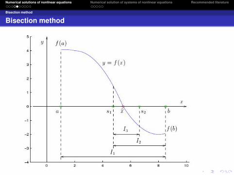
Bisection method

Let us first examine the methods that allow us to fined a small interval inwhich the solution is located.If the function f (x) in (1) is continuous then it is sufficient to find two points x ′

and x ′′ such that f (x ′)f (x ′′) < 0, i.e., such points that the function f hasdifferent signs at these two points. Then, due to the continuity of f , there is atleast one root between x ′ and x ′′. If there is exactly one root and not more inthe given interval, we call this interval the separation interval.The simplest method to decrease the interval 〈x ′, x ′′〉 containing the root isthe bisection method.Let us denote by x the center of the interval 〈x ′, x ′′〉, i.e., x = (x ′ + x ′′)/2.Then either f (x ′) · f (x) < 0 or f (x) · f (x ′′) < 0. In the former case wedecrease the interval to 〈x ′, x〉, in the latter case the new interval will be〈x , x ′′〉. After n bisection steps the size of the interval is

|x ′ − x ′′| = 2−nr , (8)

where r is the size of the original interval. After 10 bisection steps the intervalshrinks 1024 times.This method converges slowly but it is reliable and it is good when we havenot enough information about the precise location of the root.


Bisection method

Bisection method


Newton method

Newton method

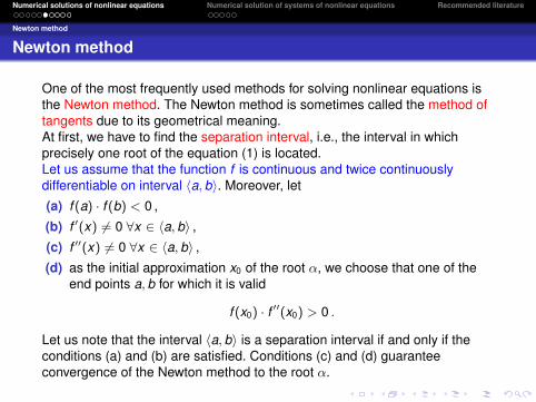
One of the most frequently used methods for solving nonlinear equations isthe Newton method. The Newton method is sometimes called the method oftangents due to its geometrical meaning.At first, we have to find the separation interval, i.e., the interval in whichprecisely one root of the equation (1) is located.Let us assume that the function f is continuous and twice continuouslydifferentiable on interval 〈a, b〉. Moreover, let

(a) f (a) · f (b) < 0 ,

(b) f ′(x) 6= 0 ∀x ∈ 〈a, b〉 ,(c) f ′′(x) 6= 0 ∀x ∈ 〈a, b〉 ,(d) as the initial approximation x0 of the root α, we choose that one of the

end points a, b for which it is valid

f (x0) · f ′′(x0) > 0 .

Let us note that the interval 〈a, b〉 is a separation interval if and only if theconditions (a) and (b) are satisfied. Conditions (c) and (d) guaranteeconvergence of the Newton method to the root α.


Newton method

Let us choose the zero approximationx0 of the root α. Geometrically, theNewton method can be described asfollows: At the point [x0, f (x0)] we con-struct the tangent to the graph of thefunction f (x). The first iteration is theintersection of this tangent with the xaxis. Hence, for the first iteration wehave

x1 = x0 −f (x0)

f ′(x0).

Now, we construct the tangent at thepoint [x1, f (x1)] and the intersection ofthis tangent with the x is the secondapproximation of the root α and so on.In general, for (n + 1)− iteration wehave the formula

xn+1 = xn −f (xn)

f ′(xn−1), n = 1, 2, . . . .

If we prescribe the accuracy ofthe calculation in advance, forexample ε = 10−4, then we willend the calculation if

|xn+1 − xn| < const · 10−4 .


Newton method

F Quadratic convergence of Newton’s method

We are looking for a root α of the equation f (x) = 0, i.e. for such α thatf (α) = 0. Let x0 be a starting approximation. Then (k + 1)−st step gives

xk+1 = xk −f (xk )

f ′(xk ), k = 1, 2, . . . .

The error of computation in k−th step is ek = α− xk ⇒ α = xk + ek .If we apply Taylor’s expansion to the function f at the point xk we obtain

f (x) = f (xk ) + f ′(xk )(x − xk ) +f ′′(xk )

2!(x − xk )2 +O(x − xk )3 ,

Let us put x := α and x − xk = α− xk = ek . Then

0 =f (α) = f (xk + ek ) = f (xk ) + f ′(xk ) · ek +12

f ′′(xk ) · e2k +O(e3

k )

−f (xk ) = f ′(xk ) · ek +12

f ′′(xk ) · e2k +O(e3

k )∣∣ : f ′(xk ) 6= 0

−f (xk )

f ′(xk )︸︷︷︸ = ek +12

f ′′(xk )

f ′(xk )e2

k +O(e3k )

xk+1 = xk − f (xk )f ′(xk )


Newton method

F

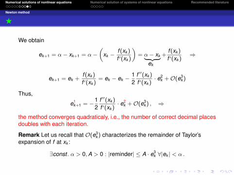
We obtain

ek+1 = α− xk+1 = α−(

xk −f (xk )

f ′(xk )

)= α− xk︸︷︷︸+

f (xk )

f ′(xk )⇒

ek

ek+1 = ek +f (xk )

f ′(xk )= ek − ek −

12

f ′′(xk )

f ′(xk )· e2

k +O(e3k )

Thus,

e1k+1 = −1

2f ′′(xk )

f ′(xk )· e2

k +O(e3k ) , ⇒

the method converges quadraticaly, i.e., the number of correct decimal placesdoubles with each iteration.

Remark Let us recall that O(e3k ) characterizes the remainder of Taylor’s

expansion of f at xk :

∃const . α > 0,A > 0 : |reminder| ≤ A · e3k ∀|ek | < α .


Newton method

F Examples for practicing

1 Verify that the interval 〈1,√

3〉 is the separation interval for solution of theequation

x + arctan x − 2 = 0 ,

and that at this interval, the Newton method can be used to solve thisequation. Select the zero approximation x0 and calculate at least oneother approximation of the root.

2 Verify that the interval 〈π2 , π〉 is the separation interval for solution of theequation

x = 6 sin x ,

and that at this interval, the Newton method can be used to solve thisequation. Select the zero approximation x0 and calculate at least oneother approximation of the root. How many other solutions does thisequation have?

3 Use an appropriate figure to find out how many roots has the equation

x ln x − 3 = 0

and for the smallest root specify a separation interval of a length of atmost 1 and the initial approximation x0 for the Newton method. Calculateat least one additional approximation by the Newton method.


Numerical solution of systems of nonlinear equations

A very common problem arising when dealing with practical problems inchemical engineering is the task to find n unknowns x1, x2, . . . , xn, whichsatisfy the following system of nonlinear equations:

f1(x1, x2, . . . , xn) = 0f2(x1, x2, . . . , xn) = 0

...fn(x1, x2, . . . , xn) = 0.

(9)

For solving of systems of nonlinear equations, there were developed severaliterative methods of the type

xk+1 = Φ(xk ), k = 0, 1, . . . , (10)

where xk is the k−th aproximation of the vector of unknownsx = (x1, x2, . . . , xn)T . Newton’s method is the most frequent one.


Newton’s method for systems of nonlinear equations


Let us denote f = (f1, . . . , fn)T. We define Jacobi matrix of functions fi (partialderivatives are evaluated at the point x) as:

J(x) =

∂f1∂x1

∂f1∂x2

. . . ∂f1∂xn

∂f2∂x1

. . .

...∂fn∂x1

∂fn∂x2

. . . ∂fn∂xn

. (11)

For Newton’s method, we choose in the equation (10) Φ as

Φ(x) = x− λJ−1(x)f(x) .

Thus,xk+1 = xk − λk J−1(xk )f(xk ). (12)

We multiply the equation (12) by the matrix J(xk ) and we obtain the final formof the Newton method, as it is practically used:

J(xk )4xk = −f(xk ) (13)

xk+1 = xk + λk4xk . (14)



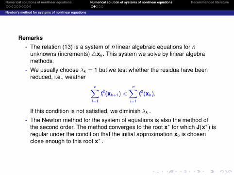
Remarks- The relation (13) is a system of n linear algebraic equations for n

unknowns (increments) 4xk . This system we solve by linear algebramethods.

- We usually choose λk = 1 but we test whether the residua have beenreduced, i.e., weather

n∑i=1

f 2i (xk+1) <

n∑i=1

f 2i (xk ).

If this condition is not satisfied, we diminish λk .

- The Newton method for the system of equations is also the method ofthe second order. The method converges to the root x∗ for which J(x∗) isregular under the condition that the initial approximation x0 is chosenclose enough to this root x∗ .


Geometric concept in R2

Geometric concept in R2

Let us consider a system of two equations for two unknowns x , y :

f1(x , y) = 0 ,

f2(x , y) = 0 .

Let (xk , yk ) be an approximation of the root (α, β) .

At the point (xk , yk , f1(xk , yk )) we construct the tangent plane to the graph ofthe function f1(x , y) and similarly, at the point (xk , yk , f2(xk , yk )) we constructthe tangent plane to the graph of the function f2(x , y) .

These two tangent planes intersect the plane z = 0 in two lines of theintersection.

The intersection of these lines is the next approximation (xk+1, yk+1) of theroot (α, β) .


Example

F Example

Let us solve the following system of nonlinear equations:

f1(x) = 16x41 + 16x4

2 + x43 − 16 = 0

f2(x) = x21 + x2

2 + x23 − 3 = 0 (15)

f3(x) = x31 − x2 = 0.

Let us choose the initial approximation x0 = (1, 1, 1) .Then

f(x0) =

1700

, J(x0) =

64 64 42 2 23 −1 0

,

x1 = x0 − J−1(x0)f(x0) =

(223240

,6380,

7960

).

For clarity, all iterations are listed in the following table. The fourthapproximation has already the precision to six decimal places.


Example

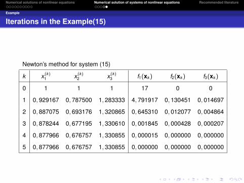
Iterations in the Example(15)

Newton’s method for system (15)

k x (k)1 x (k)

2 x (k)3 f1(xk ) f2(xk ) f3(xk )

0 1 1 1 17 0 0

1 0, 929167 0, 787500 1, 283333 4, 791917 0, 130451 0, 014697

2 0, 887075 0, 693176 1, 320865 0, 645310 0, 012077 0, 004864

3 0, 878244 0, 677195 1, 330610 0, 001845 0, 000428 0, 000207

4 0, 877966 0, 676757 1, 330855 0, 000015 0, 000000 0, 000000

5 0, 877966 0, 676757 1, 330855 0, 000000 0, 000000 0, 000000


Recommended literature

Kubıcek M., Dubcova M., Janovska D.: Numerical Methods andAlgorithms, http://old.vscht.cz/mat/Ang/NM-Ang/NM-Ang.pdf

Rasmuson A., Andersson B., Olsson L., Andersson R.: MathematicalModeling in Chemical Engineering. Cambridge University Press, 2014.

Recktenwald G.: Numerical Integration of Ordinary Differential Equationsfor Initial Value Problems. Portland State University 2007,[email protected].

Shampine L. F., Allen R, C, Jr., and Pruess S.: Fundamentals ofNumerical Computing. J. Wiley, New York 1997.

Upreti S. R.: Process Modeling and Simulation for Chemical Engineers.John Wiley & Sons Ltd. 2017.

Mathematics for chemical engineers · 2018-03-15 · Numerical solutions of nonlinear equations...

Documents

Transcript of Mathematics for chemical engineers · 2018-03-15 · Numerical solutions of nonlinear equations...