Mathematics 595 (CAP/TRA) Fall 2005

2 Metric and topological spaces

2.1 Metric spaces

The notion of a metric abstracts the intuitive concept of “distance”. It allows forthe development of many of the standard tools of analysis: continuity, convergence,compactness, etc. Spaces equipped with both a linear (algebraic) structure and ametric (analytic) structure will be considered in the next section. They providesuitable environments for the development of a rich theory of differential calculusakin to the Euclidean theory.

Definition 2.1.1. A metric on a space X is a function d : X ×X → [0,∞) which issymmetric, vanishes at (x, y) if and only if x = y, and satisfies the triangle inequality

d(x, y) ≤ d(x, z) + d(z, y) for all x, y, z ∈ X.

The pair (X, d) is called a metric space.

Notice that we require metrics to be finite-valued. Some authors consider allowinfinite-valued functions, i.e., maps d : X × X → [0,∞]. A space equipped withsuch a function naturally decomposes into a family of metric spaces (in the senseof Definition 2.1.1), which are the equivalence classes for the equivalence relationx ∼ y if and only if d(x, y) < ∞.

A pseudo-metric is a function d : X × X → [0,∞) which satisfies all of theconditions in Definition 2.1.1 except that the condition “d vanishes at (x, y) if andonly if x = y” is replaced by “d(x, x) = 0 for all x”. In other words, a pseudo-metricis required to vanish along the diagonal {(x, y) ∈ X × X : x = y}, but may alsovanish for some pairs (x, y) with x 6= y.

Exercise 2.1.2. Let (X, d) be a pseudo-metric space. Consider the relation on Xgiven by x ∼ y if and only if d(x, y) = 0. Show that this is an equivalence relation,and that the map d/ ∼ on the quotient space X/ ∼ given by

(d/ ∼)([x], [y]) := d(x, y)

is well-defined. Show that d/ ∼ is a metric on X/ ∼. The space (X/ ∼, d/ ∼) iscalled the quotient metric space for (X, d); it is a canonically defined metric spaceassociated with the given pseudo-metric space.

Every norm on a vector space defines a translation-invariant metric.

Definition 2.1.3. Let V be a vector space over F = R or F = C. A norm on V isa map || · || : V → [0,∞) so that

• (nondegeneracy) ||v|| = 0 if and only if v = 0;

• (homogeneity) ||av|| = |a| ||v|| for all a ∈ F and v ∈ V ;

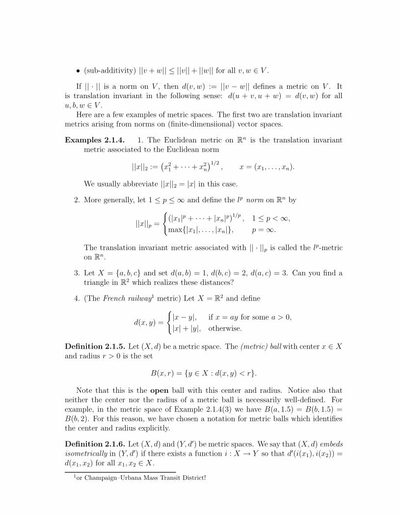
• (sub-additivity) ||v + w|| ≤ ||v||+ ||w|| for all v, w ∈ V .

If || · || is a norm on V , then d(v, w) := ||v − w|| defines a metric on V . Itis translation invariant in the following sense: d(u + v, u + w) = d(v, w) for allu, b, w ∈ V .

Here are a few examples of metric spaces. The first two are translation invariantmetrics arising from norms on (finite-dimensiional) vector spaces.

Examples 2.1.4. 1. The Euclidean metric on Rn is the translation invariantmetric associated to the Euclidean norm

||x||2 :=(

x21 + · · ·+ x2

n

)1/2, x = (x1, . . . , xn).

We usually abbreviate ||x||2 = |x| in this case.

2. More generally, let 1 ≤ p ≤ ∞ and define the lp norm on Rn by

||x||p =

{

(|x1|p + · · ·+ |xn|p)1/p , 1 ≤ p < ∞,

max{|x1|, . . . , |xn|}, p = ∞.

The translation invariant metric associated with || · ||p is called the lp-metricon Rn.

3. Let X = {a, b, c} and set d(a, b) = 1, d(b, c) = 2, d(a, c) = 3. Can you find atriangle in R2 which realizes these distances?

4. (The French railway1 metric) Let X = R2 and define

d(x, y) =

{

|x − y|, if x = ay for some a > 0,

|x| + |y|, otherwise.

Definition 2.1.5. Let (X, d) be a metric space. The (metric) ball with center x ∈ Xand radius r > 0 is the set

B(x, r) = {y ∈ X : d(x, y) < r}.

Note that this is the open ball with this center and radius. Notice also thatneither the center nor the radius of a metric ball is necessarily well-defined. Forexample, in the metric space of Example 2.1.4(3) we have B(a, 1.5) = B(b, 1.5) =B(b, 2). For this reason, we have chosen a notation for metric balls which identifiesthe center and radius explicitly.

Definition 2.1.6. Let (X, d) and (Y, d′) be metric spaces. We say that (X, d) embedsisometrically in (Y, d′) if there exists a function i : X → Y so that d′(i(x1), i(x2)) =d(x1, x2) for all x1, x2 ∈ X.

1or Champaign–Urbana Mass Transit District!

If X admits an isometric embedding in Y , then—from the point of view of metricgeometry—we may as well consider X as a subset of Y : all metric properties of Xare inherited from the ambient space Y .

The triangle inequality in Examples 2.1.4(1) and (2) is usually called the Minkowskiinequality. We prove it, as well as the fundamental Holder inequality in the followingtheorem.

Theorem 2.1.7 (Holder and Minkowski inequalities for Rn). Let v, w ∈ Rn

and let 1 ≤ p, q ≤ ∞ with1

p+

1

q= 1 (2.1.8)

(we interpret 1∞

= 0). Then

|v · w| ≤ ||v||p||w||q (2.1.9)

(where v · w denotes the usual dot product) and

||v + w||p ≤ ||v||p + ||w||p. (2.1.10)

A pair of real numbers p and q satisfying (2.1.8) is called a Holder conjugate pair.

Lemma 2.1.11 (Young’s inequality). For all Holder pairs p, q and all s, t > 0,

st ≤ sp

p+

tq

q.

There is a simple geometric argument which shows this lemma. Consider thefunction t = sp−1 in the first quadrant {(s, t) : s, t > 0}. The fact that p and qform a Holder conjugate pair means that the inverse of this function is s = tq−1.The terms sp

pand tq

qrepresent areas of certain regions bounded by the graph of this

function and the s- and t-axes, respectively. The union of these two regions containsthe rectangle [0, s] × [0, t], which proves the lemma.

Exercise 2.1.12. Fill in the details in the above argument.

Proof. First, we prove Holder’s inequality (2.1.9). By the homogeneity of the norms|| · ||p and || · ||q, it suffices to assume that ||v||p = ||w||q = 1. If v = (v1, . . . , vn) andw = (w1, . . . , wn), then

|v · w| ≤n∑

i=1

|vi| |wi| ≤∑

i

|vi|pp

+|wi|q

q

by Young’s inequality

=||v||pp

p+

||w||qqq

=1

p+

1

q= 1.

To prove Minkowski’s inequality (2.1.10), we write

||v + w||pp ≤n∑

i=1

|vi + wi|p−1(|vi| + |wi|)

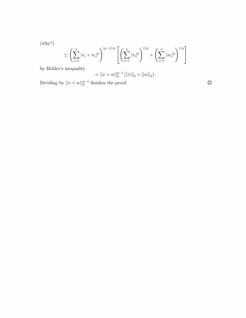
(why?)

≤(

n∑

i=1

|vi + wi|p)(p−1)/p

(

n∑

i=1

|vi|p)1/p

+

(

n∑

i=1

|wi|q)1/q

by Holder’s inequality= ||v + w||p−1

p (||v||p + ||w||q) .

Dividing by ||v + w||p−1p finishes the proof.

2.2 Maps between metric spaces

In this section we discuss classes of mappings between metric spaces. We begin withthe most well-known class, the continuous maps.

Definition 2.2.13. A map f : (X, d) → (Y, d′) between metric spaces is continuousif for every x0 ∈ X and ε > 0 there exists δ > 0 so that d(x, x0) < δ impliesd′(f(x), f(x0)) < ε.

Equivalently, f(B(x0, δ)) ⊂ B(f(x0), ε).

The reformulation of continuity in terms of the action of the map on open setswill allow us to extend the definition of continuity to a more general class of spaces(topological spaces) later in this chapter.

Definition 2.2.14. An open set in a metric space is a (possibly empty) union of(open) balls.

Notice that we make no restriction on the type (disjoint or not) or cardinality ofthe union; any union of open balls defines an open set. The empty union is allowed,i.e., the empty set is understood to be an open set.

Lemma 2.2.15. Let U be a set in X. The following are equivalent.

(1) U is an open set,

(2) For every x0 ∈ U there exists r = r(x0) > 0 so that B(x0, r) ⊂ U .

Proof. Suppose (2) is valid. Then

U ⊂⋃

x0∈U

B(x0, r(x0)) ⊂ U

so equality holds and U is a union of open balls. Thus (1) is true.For the converse, suppose that U is an open set and let x0 ∈ U . Then x0 ∈

B(x1, δ) ⊂ U for some x1 and δ > 0 and so

x0 ∈ B(x0, δ − d(x0, x1)) ⊂ B(x1, δ) ⊂ U.

Thus the condition in (2) holds for this x0 with r(x0) = δ − d(x0, x1) > 0.

Proposition 2.2.16. Let f : (X, d) → (Y, d′) be a function. The following areequivalent.

(1) f is continuous,

(2) For every open set V in Y , the preimage U = f−1(V ) is open in X.

Proof. Suppose (2) is valid and let x0 ∈ X, ε > 0 be given. Set V = B(f(x0), ε).Since V is open in Y , U = f−1(V ) is open in X, so (by Lemma 2.2.15) U is the unionof open balls centered at every point of U . In particular, there is a ball B(x0, δ) ⊂ U ,so f(B(x0, δ)) ⊂ f(U) = V = B(f(x0), ε). Hence f is continuous.

Now suppose that f is continuous, and let V be open in Y . Let x0 ∈ U :=f−1(V ) and choose ε so that B(f(x0), ε) ⊂ V . By hypothesis, there is δ so thatf(B(x0, δ)) ⊂ B(f(x0), ε) ⊂ V , i.e., B(x0, δ) ⊂ U . Since x0 was an arbitrary pointof U , U is open.

Here are some important classes of examples of continuous functions.

Definition 2.2.17. A map f : (X, d) → (Y, d′) is Lipschitz if there exists L < ∞ sothat d′(f(x1), f(x2)) ≤ Ld(x1, x2) for all x1, x2 ∈ X.

Every Lipschitz function is continuous; check that the choice δ = ε/L works forany point x0 ∈ X and ε > 0. We often emphasize this by using the term Lipschitzcontinuous.

Lipschitz functions are one of the basic workhorses of modern analysis; theirrole in the modern theory of analysis on metric spaces is comparable to the role ofsmooth functions in standard real analysis.

In many situations, it’s enough to know that a Lipschitz-type condition holds ateach point of x0 (with Lipschitz constant L depending on x0).

Definition 2.2.18. A map f : (X, d) → (Y, d′) is locally Lipschitz if for each x0 ∈ Xthere exists r > 0 so that f |B(x0,r) is Lipschitz.

Examples 2.2.19. 1. Distance functions are Lipschitz. Fix x0 ∈ X and definef : X → [0,∞) by f(x) = d(x, x0). Then f is 1-Lipschitz as a map from (X, d) toR with Euclidean metric. Indeed, for all x1, x2 ∈ X,

|f(x1) − f(x2)| = |d(x1, x0) − d(x2, x0)| ≤ d(x1, x2)

by the triangle inequality.2. Every C1 function f : R → R is locally Lipschitz. (C1 means continuously

differentiable: f ′ exists and is continuous.) To prove this, we need to use the factthat a continuous (real-valued) function defined on a closed and bounded set in R isnecessarily bounded. (We will prove a more general version of this fact later on inthese notes.) We will show that f is Lipschitz on any closed and bounded subset ofR. It’s enough to do this for any closed interval I. By the preceding remark, thereexists L < ∞ so that |f ′(x)| ≤ L for all x ∈ I. For any two points a, b ∈ I, thereexists c ∈ [a, b] so that f(b) − f(a) = f ′(c)(b − a) (Mean Value Theorem). Then

|f(b) − f(a)| ≤ L|b − a|

so f |I is Lipschitz.

Remark 2.2.20. Holder functions are generalization of Lipschitz functions. Afunction f : (X, d) → (Y, d′) is Holder (or Holder continuous) with exponent α,0 < α ≤ 1, if there exists L < ∞ so that d′(f(x1), f(x2)) ≤ Ld(x1, x2)

α for allx1, x2 ∈ X.

Exercise 2.2.21. In Problem 4(a) of Homework #3, we observed that the functiondε defines a metric on X whenever d is a metric on X. Let f : X → R be a function.Show that f : (X, d) → R is ε-Holder continuous if and only if f : (X, dε) → R isLipschitz continuous.

Definition 2.2.22. The modulus of continuity of a function f : (X, d) → (Y, d′) isthe function

ωf(r) = sup{d′(f(x), f(y)) : d(x, y) < r}.Notice that ωf may take on the value +∞.

For example, if f is Lipschitz with constant L, then ωf(r) ≤ Lr. If f is Holderwith exponent α and constant L, then ωf (r) ≤ Lrα.

Definition 2.2.23. A function f : (X, d) → (Y, d′) is uniformly continuous iflimr→0 ωf(r) = 0. Equivalently, f is uniformly continuous if for all ε > 0 thereexists δ > 0 so that for all x, x0 ∈ X, d(x, x0) < δ implies d′(f(x), f(x0)) < ε.

It’s worth reiterating how this differs from the usual notion of continuity; in thedefinition of uniform continuity the choice of δ must be made independently of thepoint x0.

To conclude this section, we discuss the Lipschitz equivalence of the lp metricson Rn.

Two metrics d and d′ on a space X are called Lipschitz equivalent if the identitymap from (X, d) to (X, d′) and its inverse are Lipschitz continuous. In a similarmanner, we define the notions of Holder equivalence, uniform equivalence, etc. Allof these notions are equivalence relations on the collection of all metrics on X.

Proposition 2.2.24. Fix n ∈ N. The lp metrics || · ||p, 1 ≤ p ≤ ∞ on Rn are allmutually Lipschitz equivalent.

Proof. It’s enough to show that || · ||p and || · ||∞ are Lipschitz equivalent. In fact,we will show that

n−1/p||x||p ≤ ||x||∞ ≤ ||x||p (2.2.25)

for all x ∈ Rn. Recall that ||x||∞ = maxi |xi| and ||x||p = (∑

i |xi|p)1/p, wherex = (x1, . . . , xn). The right hand inequality in (2.2.25) is obvious. For the left handinequality, compute

||x||pp =∑

i

|xi|p ≤ n||x||p∞

and take pth roots.

Remark 2.2.26. In fact, any two norms on a finite-dimensional vector space defineLipschitz equivalent translation invariant metrics.

Exercise 2.2.27. From (2.2.25) it easily follows that

n−1/q||x||q ≤ ||x||p ≤ n1/p||x||q

for all 1 ≤ p, q ≤ ∞ and all x ∈ Rn. However, these are not the best constants forthe Lipschitz equivalence of (Rn, || · ||p) and (Rn, || · ||q). Show that

||x||q ≤ ||x||p ≤ n1/p−1/q||x||q

for all 1 ≤ p ≤ q ≤ ∞ and all x ∈ Rn. (Hint: one direction follows from Holder’sinequality, using the Holder conjugate pairs q

pand q

q−p. For the other direction,

compare Exercise 4(a) on Homework #3.)

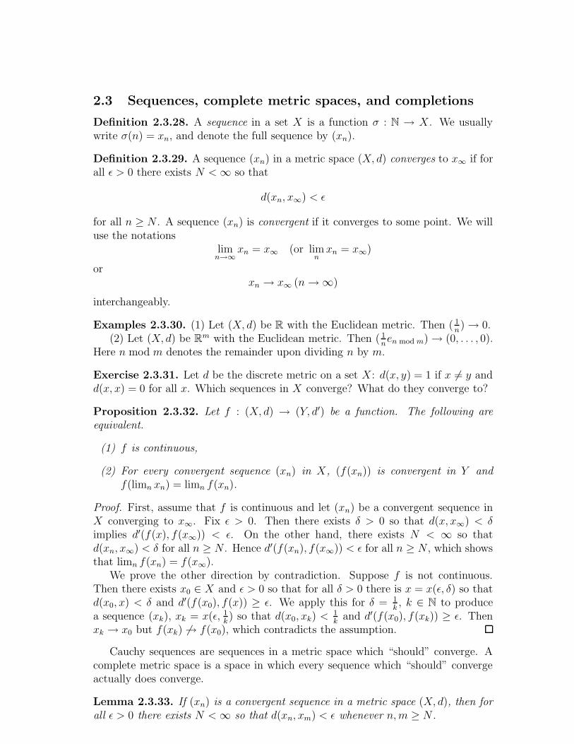
2.3 Sequences, complete metric spaces, and completions

Definition 2.3.28. A sequence in a set X is a function σ : N → X. We usuallywrite σ(n) = xn, and denote the full sequence by (xn).

Definition 2.3.29. A sequence (xn) in a metric space (X, d) converges to x∞ if forall ε > 0 there exists N < ∞ so that

d(xn, x∞) < ε

for all n ≥ N . A sequence (xn) is convergent if it converges to some point. We willuse the notations

limn→∞

xn = x∞ (or limn

xn = x∞)

orxn → x∞ (n → ∞)

interchangeably.

Examples 2.3.30. (1) Let (X, d) be R with the Euclidean metric. Then ( 1n) → 0.

(2) Let (X, d) be Rm with the Euclidean metric. Then ( 1nen mod m) → (0, . . . , 0).

Here n mod m denotes the remainder upon dividing n by m.

Exercise 2.3.31. Let d be the discrete metric on a set X: d(x, y) = 1 if x 6= y andd(x, x) = 0 for all x. Which sequences in X converge? What do they converge to?

Proposition 2.3.32. Let f : (X, d) → (Y, d′) be a function. The following areequivalent.

(1) f is continuous,

(2) For every convergent sequence (xn) in X, (f(xn)) is convergent in Y andf(limn xn) = limn f(xn).

Proof. First, assume that f is continuous and let (xn) be a convergent sequence inX converging to x∞. Fix ε > 0. Then there exists δ > 0 so that d(x, x∞) < δimplies d′(f(x), f(x∞)) < ε. On the other hand, there exists N < ∞ so thatd(xn, x∞) < δ for all n ≥ N . Hence d′(f(xn), f(x∞)) < ε for all n ≥ N , which showsthat limn f(xn) = f(x∞).

We prove the other direction by contradiction. Suppose f is not continuous.Then there exists x0 ∈ X and ε > 0 so that for all δ > 0 there is x = x(ε, δ) so thatd(x0, x) < δ and d′(f(x0), f(x)) ≥ ε. We apply this for δ = 1

k, k ∈ N to produce

a sequence (xk), xk = x(ε, 1k) so that d(x0, xk) < 1

kand d′(f(x0), f(xk)) ≥ ε. Then

xk → x0 but f(xk) 6→ f(x0), which contradicts the assumption.

Cauchy sequences are sequences in a metric space which “should” converge. Acomplete metric space is a space in which every sequence which “should” convergeactually does converge.

Lemma 2.3.33. If (xn) is a convergent sequence in a metric space (X, d), then forall ε > 0 there exists N < ∞ so that d(xn, xm) < ε whenever n, m ≥ N .

Proof. Suppose that xn → x∞. Given ε > 0 choose N so that d(xn, x∞) < 12ε

whenever n ≥ N . If n, m ≥ N , then d(xn, xm) ≤ d(xn, x∞)+ d(x∞, xm) < 12ε+ 1

2ε =

ε.

Definition 2.3.34. A sequence (xn) is Cauchy if the conclusion of Lemma 2.3.33holds. A metric space (X, d) is complete if every Cauchy sequence is convergent.

Examples 2.3.35. (1) R is complete; Q is not complete. (Why?)(2) (Rn, || · ||p) is complete for any n and any 1 ≤ p ≤ ∞. Let’s check this

for n = p = 2. Suppose that ((xn, yn)) is Cauchy in R2 (Euclidean metric). Since|xn − xm| ≤ ||(xn, yn)− (xm, ym)||2 and |yn − ym| ≤ ||(xn, yn)− (xm, ym)||2, (xn) and(yn) are Cauchy in R. Since R is complete, there exist points x∞, y∞ ∈ R so thatxn → x∞ and yn → y∞. We claim that (xn, yn) → (x∞, y∞). Given ε > 0 chooseN1 and N2 so that |xn − x∞| < ε/

√2 for all n ≥ N1 and |yn − y∞| < ε/

√2 for all

n ≥ N2. Let N be the maximum of N1 and N2. If n ≥ N then

||(xn, yn) − (xm, ym)||2 = (|xn − xm|2 + |yn − ym|2)1/2 < (2(ε/√

2)2)1/2 = ε.

This shows that (xn, yn) → (x∞, y∞), as desired.

Lemma 2.3.36. Uniformly continuous functions maps Cauchy sequences to Cauchysequences.

Proof. Let f : (X, d) → (Y, d′) be uniformly continuous and let (xn) in X be aCauchy sequence. Let ε > 0 and choose δ > 0 as in the definition of uniformcontinuity. Since (xn) is Cauchy there exists N so that d(xn, xm) < δ whenevern, m ≥ N . Then d′(f(xn), f(xm)) < ε for all such n, m, so (f(xn)) is Cauchy.

Definition 2.3.37. A set C ⊂ X is closed if X \ C is open.

Lemma 2.3.38. C is closed if and only if the following holds:

Whenever (xn) ⊂ C is a convergent sequence, then limn xn ∈ C. (2.3.39)

Proof. Suppose that C is closed and that x∞ = limn xn with (xn) ⊂ C and x∞ 6∈ C.Since X \C is open, there exists δ > 0 so that B(x∞, δ) ⊂ X \C. This implies thatd(x∞, xn) ≥ δ for all n, which contradicts the assumption that xn → x∞.

Conversely, suppose that C is not closed, but (2.3.39) holds. Then X \ C is notopen, so there exists x∞ ∈ X \ C so that for all δ > 0, B(x∞, δ) ∩ C 6= ∅. Applythis for δ = 1

k, k ∈ N to produce a sequence (xk) ⊂ C with d(x∞, xk) < 1

k. Thus

xk → x∞. Hence (xk) is a convergent sequence in C, but x∞ = limk xk ∈ X \ C,which contradicts (2.3.39).

Arbitrary intersections of closed sets are still closed, since arbitrary unions ofopen sets are still open.

Definition 2.3.40. A set A ⊂ X is dense if every nonempty open set O in X hasnonempty intersection with A.

For example, the rationals Q are dense in the reals R.

Remark 2.3.41. By Lemma 2.2.15, A is dense in X if and only if every open ballB(x0, r) has nonempty intersection with A. Choosing r = 1

kfor each k ∈ N, we

obtain that A is dense in X if and only if every point in X is the limit of a sequencefrom A.

Definition 2.3.42. Let A ⊂ X. The closure of A is A =⋂

C closed:A⊂CC.

Being an intersection of closed sets, the closure of a set is a closed set. ClearlyA ⊂ A for any A.

Lemma 2.3.43. For any set A ⊂ X, A is dense in A.

Proof. Suppose not. Then there exists O open in X so that O∩A 6= ∅ but O∩A = ∅.Let C = X \ O; C is a closed set. Since O ∩ A = ∅, A ⊂ C ∩ A. Since O ∩ A 6= ∅,C ∩ A ( A. Since C ∩ A is closed, we have contradicted the definition of A.

We now turn to the notion of the completion of a (non-complete) metric space.We give the traditional definition via equivalence classes of Cauchy sequences. Inthe next section, we give an alternate description of the completion which is morealgebraic.

Definition 2.3.44. Given two sequences x = (xn) and y = (yn) in a set X, we candefine a new sequence x∨ y = (zn) by setting z2n−1 = xn and z2n = yn for all n ∈ N.This interleaves the elements of the sequences x and y. We call x ∨ y the join of xand y.

We now define an equivalence relation on the set of all Cauchy sequences in ametric space (X, d): two such sequences x and y are equivalent if and only if x ∨ yis Cauchy. We denote the set of equivalence classes for this equivalence relation byX, and call it the completion of X.

Notice that the notation which we use for the completion is the same as thatwhich we used for the closure of a set. After Theorem 2.3.47 this will cause noconfusion.

Exercise 2.3.45. Show that the relation in this definition is in fact an equivalencerelation.

Note that there is a natural embedding ι of X into X given by x 7→ (x, x, x, . . .).We now want to equip the completion with a metric so that this becomes an isometricembedding.

Lemma 2.3.46. The function d : X×X → [0,∞) given by d([x], [y]) = limn d(xn, yn),x = (xn), y = (yn), is well-defined.

Proof. It’s enough to show that if x = (xn) ∼ z = (zn) and y = (yn) are Cauchysequences, then limn d(xn, yn) = limn d(zn, yn). By the triangle inequality, this willfollow if we can show limn d(xn, zn) = 0. Since x ∼ z, x∨ z =: w = (wn) is a Cauchysequence. In other words, for all ε > 0 there exists N so that m, n ≥ N impliesd(wn, wm) < ε. We may assume that N = 2M +1 is odd. From the definition of thejoin, we have

d(xn, xm) < ε, d(xn, zm) < ε, and d(zn, zm) < ε

for all n, m ≥ M . In particular, d(xn, zn) < ε for all n ≥ M . Thus limn d(xn, zn) =0.

Another way to think about this is as a quotient metric space arising from apseudometric space (see Exercise 2.1.2). In fact, the collection of all Cauchy se-quences in (X, d), with the metric d from the lemma, forms a pseudometric space,and (X, d) is precisely the quotient metric space.

Theorem 2.3.47. 1. (X, d) is a complete metric space,

2. the embedding ι : X → X given above is an isometric embedding so that ι(X)is dense in X.

The proof is an abstract version of the classical argument used to construct thereal numbers as a completion of the rational numbers. In the next section, we willgive an alternate description of the completion of a metric space (X, d) as a subsetof a certain space of functions defined on X.

Proof. We omit the proof that d is a metric on X. The completeness of (X, d) willfollow once we prove part 2, using Lemma 2.3.48. (Apply the lemma with A = ι(X)and Z = X, and observe that if (xn) is a Cauchy sequence in X, then ([ι(xn)])converges to [(x1, x2, x3, . . .)].)

The fact that ι is an isometric embedding is obvious, since ι(x) is the constantsequence (x, x, x, . . .) and d([x], [y]) = limn d(xn, yn).

Let ε > 0 and let [x] ∈ X. Since x = (x1, x2, . . .) is Cauchy, there exists N sothat d(xn, xm) < ε for all n, m ≥ N . Let oy = (xN , xN , xN , . . .) = ι(xN ). Then

d([x], [y]) = limn

d(xn, yn) = limn

d(xn, xN ) ≤ ε,

so B([x], ε) ∩ ι(X) 6= ∅. By Remark 2.3.41, ι(X) is dense in X.

Lemma 2.3.48. Let (Z, d) be a metric space, and let A ⊂ Z be a dense subset.Suppose that every Cauchy sequence in A converges to some element of Z. Then(Z, d) is complete.

Proof. The proof is a classical diagonal argument in the spirit of Cantor. Supposethat (zm) is a Cauchy sequence in Z. Since A is dense in Z, each zm is the limit ofa Cauchy sequence (amn) in A. We now make a diagonal construction. For each m,choose Nm so that d(amn, amn′) < 2−m whenever n, n′ ≥ Nm. Consider the sequence(amNm

). Given ε > 0, pick M so that 2−M < ε/3 and d(zm, zm′) < ε/3 wheneverm, m′ ≥ M . Since d(amNm

, zm) = limn d(amNm, amn) ≤ 2−M < ε/3, we conclude

that

d(amNm, am′Nm′

) ≤ d(amNm, zm) + d(zm, zm′) + d(zm′, am′Nm′

) <ε

3+

ε

3+

ε

3= ε.

Thus (amNm) is a Cauchy sequence in A. By assumption, it converges to some

element z ∈ Z. It’s easy to check (exercise) that limm zm = z. Hence (Z, d) iscomplete.

Proposition 2.3.49. Let A be dense in (X, d) and let f : A → (Y, d′) be a uniformlycontinuous function valued in a complete metric space. Then there exists a uniqueuniformly continuous function f : X → Y so that f |A = f |A. Moreover, the modulusof continuity of the extension agrees with that of the original function:

ωf = ωf . (2.3.50)

Proof. By Remark 2.3.41, each x ∈ X is the limit of a sequence (an) from A.Define f(x) = limn f(an). Notice that the limit exists since (an) is Cauchy, hence(by Lemma 2.3.36) (f(an)) is Cauchy, hence (since (Y, d′) is complete) (f(an)) is aconvergent sequence. We need to show that the limit is independent of the choiceof sequence. Let (bn) be another sequence in A with limit x and let ε > 0. Chooseδ > 0 so that d(x1, x2) < δ, x1, x2 ∈ A, implies d(f(x1), f(x2)) < ε. Choose N sothat

d(an, x) <δ

2

and

d(bm, x) <δ

2

for all n, m ≥ N . Thus d(an, bm) < δ so d(f(an), f(bm)) < ε for all n, m ≥ N .Sending n → ∞ gives d(f(x), f(bm)) < ε for all m ≥ N . Thus limm f(bm) = f(x).If x ∈ A we may choose (an) to be the constant sequence an = x, which shows thatf |A = f |A. Finally, let us show (2.3.50). Given x1, x2 ∈ X with d(x1, x2) < δ, wemay choose (an) and (bn) in A converging to x1 and x2 respectively. We may as wellassume that

max{d(an, x1), d(bn, x2)} <δ − d(x1, x2)

2

for all n. Then, for all n ∈ N, we have

d(an, bn) ≤ d(an, x1) + d(x1, x2) + d(x2, bn) < δ

sod′(f(x1), f(x2)) = lim

nd′(f(an), f(bn)) ≤ ωf(δ).

Thus ωf ≤ ωf ; the other direction is trivial.

Theorem 2.3.51. The completion of a metric space is unique, in the followingsense. If (Y, d′) is a complete metric space and ι′ : (X, d) → (Y, d′) is an isometricembedding so that ι′(X) is dense in Y , then there exists an isometry I of (X, d) onto(Y, d′) so that I ◦ ι = ι′.

Proof. The map ι′ ◦ ι−1 : ι(X) → Y is an isometric embedding, hence 1-Lipschitz.By Proposition 2.3.49, there exists a 1-Lipschitz map I : (X, d) → (Y, d′) so thatI ◦ ι = ι′. Similarly ι ◦ (ι′)−1 : ι′(X) → X is an isometric embedding, hence 1-Lipschitz, so there exists a 1-Lipschitz map J : (Y, d) → (X, d) so that J ◦ ι′ = ι.Composing these formulas gives J ◦ I = id on ι(X) and I ◦ J = id on ι′(X). Thisimplies that I|ι(X) is an isometry onto its image, hence I is an isometry. SimilarlyJ is an isometry; since J is the inverse of I we conclude that I is onto.

2.4 Function spaces

In this section, we introduce the notion of function spaces, i.e., spaces of functionsbetween metric spaces, which we equip with various metrics. The goal of this sectionis to prove a theorem characterizing the completion of a metric space (X, d) as asubset of a particular function space over X.

The basic function space which we consider is the space of all continuous functionsbetween two metric spaces.

Definition 2.4.52. For metric spaces (X, d) and (X ′, d′), let

C(X, Y ) = {f : X → Y | f is continuous}be the space of all continuous functions from (X, d) to (Y, d′).

A “natural” distance function to consider on this space is the maximum metric

d∞(f, g) = supx∈X

d′(f(x), g(x)).

This satisfies all of the properties of a metric except that it may take on the value+∞. For example, the distance between the functions f(x) = 1 and g(x) = x(X = Y = R) is +∞. For this reason, we will most often work with the followingsubspace of C(X, Y ).

Definition 2.4.53. Let (X, d) and (Y, d′) be metric spaces and let y0 ∈ Y . Wedefine

Cb(X, Y ) = {f ∈ C(X, Y ) : supx∈X

d′(f(x), y0) < ∞}

to be the space of all bounded continuous functions from (X, d) to (Y, d′).

Notice that, while the definition of Cb(X, Y ) depends on the choice of y0, theset of functions so obtained remains the same if y0 is changed. Indeed, if y1 ∈ Y isanother point, then

∣

∣

∣

∣

supx∈X

d′(f(x), y0) − supx∈X

d′(f(x), y1)

∣

∣

∣

∣

≤ d′(y0, y1) < ∞.

Exercise 2.4.54. Show that the maximum metric d∞ is a metric on Cb(X, Y ).

Example 2.4.55. Let X = {a, b} be a space of two points, with the discrete metricd(a, b) = 1, and let Y = R. Then every function from X to Y is continuous andbounded. In fact, we can identify Cb(X, R) with R2 by identifying f with its range(f(a), f(b)). In this case, (Cb(X, R), d∞) is isometric with (R2, ||·||∞) (the l∞ metric).

Remark 2.4.56. Suppose that (Y, d′) = (V, || · ||) is a vector space over F = R

or F = C equipped with a translation invariant metric arising from a norm. ThenCb(X, Y ) has the structure of a vector space, and d∞ is a translation invariant metricarising from a norm on Cb(X, Y ). The vector space structure on Cb(X, Y ) is givenby

(αf + βg)(x) = αf(x) + βg(x),

where f, g ∈ Cb(X, Y ), x ∈ X and α, β ∈ F, while the norm on Cb(X, Y ) is given by

||f || = supx∈X

||f(x)||.

Exercise 2.4.57. Verify the claims in the preceding remark.

A special case in the above definitions is (Y, d′) = R, i.e., the case of real-valuedfunctions on (X, d). In this case, we abbreviate

C(X, R) = C(X), and Cb(X, R) = Cb(X).

We are now ready to give an alternate description of the completion of a metricspace as a subset of the function space Cb(X). The embedding of (X, d) in Cb(X)in (2.4.60) is due to Kuratowski.

We need the following elementary lemma.

Lemma 2.4.58. Every closed subset of a complete metric space is complete (in theinduced metric).

Proof. Let (X, d) be a complete metric space, and let C be a closed subset of X.Let (xn) be a Cauchy sequence in C. Since (X, d) is complete, (xn) converges to alimit x∞ in X. Since C is closed, x∞ ∈ C. Thus (C, d) is complete.

Theorem 2.4.59. Let (X, d) be a metric space and (Y, d′) be a complete metricspace. Then (Cb(X, Y ), d∞) is a complete metric space.

Proof. Suppose that (fn) is a Cauchy sequence of bounded continuous functionswith respect to d∞. Then (fn(x)) is a Cauchy sequence in Y for each x ∈ X; by thecompleteness of Y there exists f(x) = limn fn(x). We must show that f ∈ Cb(X, Y ),and that d∞(fn, f) → 0.

Let ε > 0, and choose N so that

d∞(fn, fm) <ε

6

for all n, m ≥ N . For each x ∈ X we may choose m = m(x) ≥ N so that

d′(fm(x), f(x)) <ε

6.

Thend′(fn(x), f(x)) <

ε

3for all n ≥ N and x ∈ X, so

supn≥N

d∞(fn, f) <ε

3.

Thus d∞(fn, f) → 0. Moreover, if δ > 0 is chosen so that d(x, x1) < δ impliesd′(fN(x), fN(x1)) < ε/3, then

d′(f(x), f(x1)) ≤ d′(f(x), fN(x)) + d′(fN (x), fN(x1)) + d′(fN(x1), f(x1))

<ε

3+

ε

3+

ε

3= ε.

Thus f is continuous. Finally,

supx

d′(f(x), y0) ≤ supx

d′(fN (x), y0) + d∞(f, fN) < ∞

so f ∈ Cb(X, Y ).

We now fix a point x0 ∈ X and consider the map e from (X, d) to (C(X), d∞)given by

e(x)(y) = d(x, y) − d(x0, y). (2.4.60)

Proposition 2.4.61. The map e is an isometric embedding of (X, d) into (Cb(X), d∞).

Proof. First, we check that e(x) is a bounded function for each x ∈ X. This isimmediate from the triangle inequality:

supy∈X

|e(x)(y)| = supy∈X

|d(x, y) − d(x0, y)| ≤ d(x, x0) < ∞.

Next, we check that e is an isometry. On the one hand, we have

d∞(e(x1), e(x2)) = supy

|e(x1)(y) − e(x2)(y)| = supy

|d(x1, y) − d(x2, y)| ≤ d(x1, x2).

On the other hand,

d∞(e(x1), e(x2)) ≥ |e(x1)(x2) − e(x2)(x2)| = d(x1, x2).

Theorem 2.4.62. (e(X), d∞) is isometric with the completion (X, d) (defined inthe previous section).

Proof. By Lemma 2.4.58, the closure of e(X) in Cb(X) is complete with respect tothe metric d∞. Now the conclusion follows from the uniqueness up to isometry ofthe completion (X, d).

One disadvantage of the Kuratowski embedding is that the receiving space Cb(X)depends on the source space X.

Definition 2.4.63. A metric space is separable if it admits a countable dense subset.

For example, Rn is separable for each n.

Definition 2.4.64. The space `∞ consists of all bounded sequences of real numbers,e.g., x = (xn) ∈ `∞ if and only if xn ∈ R for all n and supn |xn| < ∞. We equip `∞

with the maximum metric

d∞(x, y) = supn

|xn − yn|, x = (xn), y = (yn).

Exercise 2.4.65. Prove that (`∞, d∞) is complete but not separable.

The embedding in the following theorem is due to Frechet. It exhibits a universalembedding space for separable metric spaces.

Theorem 2.4.66. Every separable metric space admits an isometric embedding in(`∞, d∞).

Observe that the target space in this theorem is universal, i.e., does not dependon the source. One potential criticism, however, is that this target is itself notseparable. There do exist separable metric spaces which contain isometric copies ofevery separable metric space. We do not discuss this in these notes.

Proof. Let {x1, x2, . . .} be a countable dense subset of X. Define i : X → `∞ by

i(x)n = d(x, xn) − d(x0, xn).

Observe that

||i(x) − i(y)||∞ = supn

|d(x, xn) − d(y, xn)| ≤ d(x, y)

for all x, y ∈ X. Conversely, let x, y ∈ X. There exists a subsequence xn1, xn2

, . . .which converges to y. Then

d(x, y) = limk→∞

|d(x, xnk) − d(y, xnk

)| ≤ supn

|d(x, xn) − d(y, xn)| = ||i(x) − i(y)||∞.

Thus i is an isometric embedding.

The embedding in Theorem 2.4.66 is due to Frechet.We will discuss other embedding theorems for metric spaces in Part III of these

notes.

2.5 A famous example

In this section we want to identify the completion of C([0, 1]) with respect to themetric

d1(f, g) = ||f − g||1 =

∫ 1

0

|f(t) − g(t)| dt.

The integration here is in the sense of Riemann.Let us denote the completion C([0, 1]) by L. Elements of L are equivalence classes

of Cauchy sequences of continuous functions on [0, 1]; it is not clear yet whether theycan be identified with actual functions on [0, 1]. By the end of this section, we willunderstand in what sense such an identification can be made. Until then, we’lldenote the metric in the completion by d1 rather than || · ||1 to avoid confusion. Wewill say that a sequence (fn) converges in L to a limit f if d1(fn, f) → 0.

We begin by observing that the (Riemann) integral, thought of as a continuouslinear functional on C([0, 1]), can be extended to a continuous linear functional onL. Let us write

I(f) = ||f ||1 =

∫ 1

0

f(t) dt.

Observe that I is a 1-Lipschitz linear map from C([0, 1]) to R:

|I(f) − I(g)| ≤∫ 1

0

|f(t) − g(t)| dt = d1(f, g).

Lemma 2.5.67. I can be extended to a 1-Lipschitz linear map from L to R. Fur-thermore, f ≥ 0 implies I(f) ≥ 0 for all f ∈ L.

In the preceding lemma, we gave an inequality of the form f ≥ 0 for an elementf ∈ L. The meaning of this inequality is not immediately clear. We say that f ≥ 0,f ∈ L, if f is the limit in (C([0, 1]), || · ||1) of a sequence of positive continuousfunctions. For f, g ∈ L, we say that f ≤ g if g − f ≥ 0.

Proof. The existence of the extended map I : L → R and its regularity (1-Lipschitz)are an easy application of Proposition 2.3.49. Linearity of the extension followsfrom linearity of the original map I : C([0, 1]) → R by passing to the limit. Asimilar argument establishes the coercivity estimate: f ≥ 0 implies I(f) ≥ 0 for allf ∈ L.

Elements of L are equivalence classes [(fn)] of Cauchy sequences of continuousfunctions on [0, 1] (relative to || · ||1). By the lemma, to each such equivalence classf there corresponds a number (the “integral” of f); this correspondence is linear,monotone and 1-Lipschitz from (L, || · ||1) to R. This extension of the Riemannintegral is called the Daniell integral. A different, but equivalent, approach to com-pleting the Riemann integral, due to Lebesgue, consists in first defining a notionof measure, then proceeding via the direct construction of Lebesgue measure, opensets, and then (Lebesgue) measurable and integrable functions. We will say moreabout the Lebesgue theory at the end of this section.

Theorem 2.5.68 (Monotone Convergence Theorem). Let (fn) be an increasingsequence of elements of L so that supn I(fn) < ∞. Then there exists f ∈ L so thatfn converges in L to f and I(f) = limn I(fn).

Notice that all of the elements fn, n = 1, 2, 3, . . ., and f are elements of L, henceequivalence classes of Cauchy sequences in X.

Proof. By monotonicity, (I(fn)) is an increasing sequence of real numbers which isbounded above. Hence L = limn I(fn) exists. For all ε > 0 there exists N so that

L − ε < I(fN) ≤ I(fn) ≤ L

for all n ≥ N . It follows that (fn) is a Cauchy sequence in (L, d1): n, m ≥ N implies

d1(fn, fm) = I(|fn − fm|) = I(fn) − I(fm) < ε.

Completeness of (L, d1) yields the limit element f ∈ L. The final claim comes fromthe continuity of the integral, see Lemma 2.5.67.

Now we’re prepared to show how the elements of L can be viewed as functions. Todo this, it’s necessary to pass to another quotient space, i.e., to impose an equivalencerelation on the space of functions from [0, 1] to R. To get a handle on this equivalencerelation, let’s begin with the following natural question: if (fn) is a sequence inC([0, 1]) converging in L to the zero function f∞(x) ≡ 0, how large can the set ofpoints x ∈ [0, 1] be on which fn(x) does not converge to 0?

Example 2.5.69. The sequence fn(x) = xn shows that convergence of (fn(x)) tozero can fail at a single point (x = 1).

Exercise 2.5.70. Show that convergence of (fn(x)) to zero can fail at a countableset of points.

The length |U | of an open interval U = (a, b) ⊂ R is equal to b − a.

Definition 2.5.71. A set A ⊂ [0, 1] is said to have measure zero if for all ε > 0 thereexists a collection of open intervals Ui, i ∈ N, so that A ⊂ ∪iUi and

∑

i |Ui| < ε.

Examples 2.5.72. 1. The rationals Q ∩ [0, 1] have measure zero. In fact, forany ε > 0 the sequence of open intervals Ui = (qi − 2−i−1ε, qi + 2−i−1ε) coversQ∩ [0, 1] = {q1, q2, . . .} and has

∑

i |Ui| = ε/2. (The same argument shows that anycountable subset of [0, 1] has measure zero.)

2. [0, 1] does not have measure zero. In fact, if {Ui} is any collection of openintervals with [0, 1] ⊂ ∪iUi, then

∑

i |Ui| ≥ 1. To prove this, we appeal to the Heine-Borel theorem, which we will state and prove in the following section. It impliesthat [0, 1] is compact: from every collection of open intervals covering [0, 1] we canselect a finite subcollection which still covers [0, 1]. Choose such a subcollectionUi1 , . . . , Uik . Then

∑

i

|Ui| ≥k∑

j=1

|Uij | ≥ 1

by an easy induction using the triangle inequality.3. The standard 1

3Cantor set C ⊂ [0, 1] has measure zero. Recall that

C = [0, 1] \∞⋃

m=0

⋃

i∈Im

Omi, Omi =

(

3i + 1

3m+1,3i + 2

3m+1

)

,

where Im consists of those integers i with 0 ≤ i < 3m whose ternary expansioninvolves only the digits 0 and 2. (For example, I2 = {0, 2, 6, 8}.) Observe that withthis definition for Im, all of the open intervals Omi, m ≥ 0, i ∈ Im are disjoint.Alternatively, C can be described as the set of all real numbers in [0, 1] which havea ternary expansion involving only the digits 0 and 2. C is an uncountable subsetof [0, 1] of zero length, in the sense that

∑

m

∑

i∈Im

|Omi| = 1.

To see that C has measure zero, it’s helpful to rewrite C as a decreasing intersectionof closed sets:

C =

∞⋂

m=0

⋃

i∈Im

Ami, Ami =

[

3i

3m,3i + 1

3m

]

,

where Im is as before.Suppose that 0 < ε < 1, and choose m so that

(

2

3

)m

<1

3ε.

For each i ∈ Im, let

Umi =

(

3i − ε

3m,3i + 1 + ε

3m

)

⊃ Ami.

Then C ⊂ ⋃i∈ImUmi and

∑

m

∑

i∈Im

|Umi| = (#Im)

(

1 + 2ε

3m

)

= (1 + 2ε)

(

2

3

)m

< ε.

Since ε was arbitrary, C has measure zero.4. The measure zero property is hereditary: if A has measure zero and B ⊂ A,

then B has measure zero.

Proposition 2.5.73. Let A ⊂ [0, 1] be a closed set. Then A has measure zero if andonly if there exists a sequence (fn) in C([0, 1]) converging in L to the zero functionso that A = {x : fn(x) does not converge to 0}.

A property P of real numbers is said to hold almost everywhere (a.e.) if {x ∈[0, 1] : P does not hold at x} has measure zero. With this terminology, the reverseimplication in Proposition 2.5.73 can be stated as follows: convergence in L impliespointwise convergence almost everywhere.

Exercise 2.5.74. Prove Proposition 2.5.73.

As a corollary of the preceding theorem, we see that elements of L can be iden-tified with functions on [0, 1], up to modification on sets of measure zero.

Theorem 2.5.75. Let f ∈ L. Then there exists a sequence of functions (fn) ⊂C([0, 1]) converging to f in L which converge pointwise almost everywhere to a func-tion which we denote by f(x). If (gn) is another sequence converging to f in L andpointwise to g(x) almost everywhere, then g(x) = f(x) a.e.

Proof. Choose a sequence of functions (fn) in C([0, 1]) so that d1(fn, f) < 4−n forall n. For each n¡ let

On = {x ∈ [0, 1] : |fn(x) − fn+1(x)| > 2−n}.

This is the pullback of the open set (2−n,∞) by the continuous function |fn − fn+1|,hence is open. We may then write On =

⋃

m Unm for some disjoint open intervalsUnm = (anm, bnm). Observe that

∑

m

|Umn| ≤∑

m

∫ bnm

anm

2n|fn(x) − fn+1(x)| dx

≤ 2n||fn − fn+1||1≤ 2n(d1(fn, f) + d1(fn+1, f)) < 21−n.

Let A =⋂

n≥1

⋃

k≥n Ok. For each n, A can be covered by the open intervals com-

prising⋃

k≥n Ok, which have total length at most∑

k≥n 21−k = 22−n. Thus A hasmeasure zero.

If x ∈ [0, 1] \ A, then there exists N ≥ 1 so that x /∈ ⋃

n≥N On, i.e., x ∈⋂

n≥N [0, 1] \ On. Thus |fn(x) − fn+1(x)| ≤ 2−n for all n ≥ N , so

|fn(x) − fm(x)| ≤m−1∑

k=n

|fk(x) − fk+1(x)| ≤m−1∑

k=n

2−k < 21−n ≤ 21−N

for all m > n ≥ N . Thus (fn(x)) is a Cauchy sequence in R, and so convergesto a value which we denote f(x). In other words, (fn) converges pointwise almosteverywhere to a function f(x).

Now suppose that (gn) is another sequence in C([0, 1]) converging to f in L andconverging pointwise almost everywhere to a function g(x). Passing to a subse-quence, which we continue to denote by (gn), we may assume that d1(gn, f) < 4−n

for all n. LetVn = {x ∈ [0, 1] : |gn(x) − fn(x)| > 2−n}.

Again, Vn is open since |gn − fn| is continuous. Arguing as before, we find that B =⋂

n≥1

⋃

k≥n Vk has measure zero. On the complement of B we have |gn(x)−fn(x)| →0. Since fn(x) → f(x) for all x ∈ [0, 1] \ A, f(x) = g(x) for x ∈ [0, 1] \ (A ∪ B).Thus g = f a.e.

The preceding theorem shows that elements of L can be identified with equiv-alence classes of functions, where the equivalence relation is equality almost every-where. The resulting quotient space L = L/ ∼ is called the space of (Lebesgue)

integrable functions. The linear functional I : L → R which extends the Riemannintegral on C([0, 1]) descends to a map on L which we continue to denote by I. Thequantity I(f) is called the Lebesgue integral of f over [0, 1].

Remark 2.5.76. The approach to the Lebesgue integral developed in this section(beginning with the space L of integrable functions) is somewhat unorthodox. Themore traditional development of the subject begins with the notion of Lebesguemeasure µ, which extends the usual length measure for intervals to a wider classof subsets of [0, 1]. Then a notion of integration with respect to µ can be defined,

giving a linear functional f 7→∫ 1

0f dµ on a certain completion of C([0, 1]). The

Lebesgue space L consists of all functions f for which∫ 1

0f dµ exists and is finite.

Exercise 2.5.77. Construct the Lebesgue measure µ from the space L of Lebesgueintegrable functions f with integral I(f) as defined in this section. More precisely, letΣ be the collection of all subsets E ⊂ [0, 1] whose characteristic function χE belongsto L (i.e., χE agrees a.e. with some function g ∈ L). Then define µ(E) = I(χE).Show that

• Σ is a σ-algebra: E, F ∈ Σ ⇒ E ∩ F, E ∪ F, E \ F ∈ Σ,

• µ(E ∩ F ) + µ(E ∪ F ) = µ(E) + µ(F ) for all E, F ∈ Σ,

• µ(E) = 0 if and only if E has measure zero,

• µ(⋃

m Em) =∑

m µ(Em) if (Em) is a collection of disjoint sets in Σ,

• Σ contains all open intervals, and µ(U) = d − c if U = (c, d).

One final remark is worth mentioning. In the approach taken here, the integralI(f), f ∈ L, is defined abstractly; it is not clear how to recover its value from theactual values taken on by (a representative of) f . In the alternate approach to theLebesgue integral discussed in Remark 2.5.76, the value of the integral is determinedexplicitly in terms of the actual values taken on by the function.

2.6 Compactness

Compactness is arguably the single most important concept in analysis. It is theessential feature which guarantees the existence of limits in a wide variety of cases.There are several definitions of compactness which are all equivalent in the settingof metric spaces. Some of these definitions can be extended to the more generalclass of topological spaces (see section 2.8) where they give different notions.

Definition 2.6.78. A collection {Ui}i∈I of subsets of a set X is a cover of X ifX =

⋃

i∈I Ui. A subcover of a cover {Ui}i∈I is a subcollection {Ui}i∈I′, I ′ ⊂ I, forwhich X =

⋃

i∈I′ Ui.A cover {Ui} of a metric space (X, d) is an open cover if the sets Ui are open

sets.

Definition 2.6.79. A metric space (X, d) is compact if every open cover admits asubcover of finite cardinality.

To illustrate the strength of this notion, we next present a number of propertiesof compact spaces.

Definition 2.6.80. A metric space (X, d) is bounded if X = B(x0, r) for somex0 ∈ X and r > 0. It is totally bounded if for every ε > 0 there exists a finitecollection of open balls of radius ε covering X. (The centers of such a collection ofballs are called an ε-net in (X, d).)

A sequence (xn) subconverges to x∞ if there exists a subsequence (xnk) which

converges to x∞; (xn) is subconvergent if it has a convergent subsequence. (X, d) issequentially compact if every sequence is subconvergent.

(X, d) has the finite intersection property if every collection {Fi}i∈I of closed setsin X, with the property that every finite subcollection has nonempty intersection,necessarily has nonempty intersection:

∀I ′ ⊂ I, I ′ finite⋂

i∈I′

Fi 6= ∅ ⇒⋂

i∈I

Fi 6= ∅.

Proposition 2.6.81. All compact metric spaces are

(a) bounded,

(b) totally bounded,

(c) separable,

(d) sequentially compact,

(e) complete.

Moreover, they

(f) have the finite intersection property.

Finally,

(g) closed subsets of compact spaces are compact,

(h) continuous images of compact spaces are compact,

(i) a continuous real-valued function defined on a compact metric space achievesits maximum and minimum, and

(j) continuous maps from compact spaces are uniformly continuous.

Proof. (a) Fix x0 ∈ X and consider the sequence of open sets Un = B(x0, n).(b) Consider the collection of open sets Ux = B(x, ε), x ∈ X.(c) Apply the total boundedness condition for ε = 1

k, k ∈ N, to construct finite

1k-nets Nk for each k. Then

⋃∞k=1 Nk is a countable dense set.

(d) Suppose that (xn) is a non-subconvergent sequence in (X, d). Then for eachx ∈ X, there exists εx > 0 so that B(x, εx) contains only finitely many terms in thesequence. By compactness, there is a finite subcover {B(x1, εx1

), . . . , B(xN , εxN)}

of the cover {B(x, εx)}x∈X . This subcover can contain at most finitely many termsfrom the sequence. It follows that the sequence (xn) has finite range; only finitelymany values are taken on by the elements of the sequence. Then (xn) has a constant(hence convergent) subsequence.

(e) Let (xn) be a Cauchy sequence. By sequential compactness, (xn) subconvergesto x∞ in X. But a Cauchy sequence which subconverges to x∞, necessarily convergesto x∞. Thus (X, d) is complete.

(f) Take complements!(g) Let A be a closed subset of X, and let (xn) be a sequence in A. Then (xn)

subconverges to x∞ in X. Since A is closed, x∞ ∈ A. Thus (xn) subconverges tox∞ in A, so A is compact.

(h) Let f : (X, d) → (Y, d′) be continuous, and let {Vi}i∈I be an open cover of Y .Then {Ui}i∈I , Ui = f−1(Vi), is an open cover of X, so there exists a finite subcover{Ui1 , . . . , UiN}. Then {Vi1 , . . . , ViN} is a finite subcover of Y .

(i) Let f : (X, d) → R be continuous, with (X, d) compact. By (h), f(X) ⊂ R

is compact. By the Heine–Borel theorem 2.6.84, f(X) is closed and bounded. Thussupx∈X f(x) and infx∈X f(x) are achieved, i.e., there exist points x± ∈ X so thatf(x+) = maxx∈X f(x) and f(x−) = minx∈X f(x).

(j) Let ε > 0. For each x ∈ X there exists δx > 0 so that f(B(x, 2δx)) ⊂B(fx, ε/2). The sets Ux = B(x, δx) form an open cover of X; choose a finite subcoverUx1

, . . . , UxN. Let δ = min{δx1

, . . . , δxN}. If d(x, y) < δ, then there exists i, 1 ≤ i ≤

N , so that x, y ∈ B(xi, 2δxi). Then fx, fy ∈ B(fxi, ε/2) so d(fx, fy) < ε.

The following theorem gives some of the equivalent notions of compactness inmetric spaces.

Theorem 2.6.82. Let (X, d) be a metric space. The following are equivalent:

(i) (X, d) is compact,

(ii) (X, d) has the finite intersection property for countable families {Fi}∞i=1 ofclosed sets,

(iii) (X, d) is sequentially compact,

(iv) (X, d) is complete and totally bounded.

Proof. We have already shown that (i) implies (ii), (iii) and (iv). To complete thechain of implications, we will prove that (ii) ⇒ (iii) ⇒ (iv) ⇒ (i).

(ii) ⇒ (iii): Assume that (X, d) has the finite intersection property for countablecollections {Fi}∞i=1 of closed sets. We make use of the following elementary lemma,whose proof we leave to the reader.

Lemma 2.6.83. Let (xn) be a sequence of distinct elements of (X, d), and let A ={x1, x2, . . .} be the range of this sequence. Then every element of A \A arises as thelimit of a subsequence of (xn).

Returning to the proof, suppose that (X, d) is not sequentially compact. Thenthere exists a sequence (xn) with no convergent subsequence. We may assume thatthe elements of (xn) are all distinct. By the lemma, the sets FN = {xN , xN+1, . . .},N ≥ 1, are all closed. Moreover, finite intersections of these sets are nonempty. But⋂

N FN = ∅. This contradicts the assumption.(iii) ⇒ (iv): First, suppose that (xn) is a Cauchy sequence in (X, d). By assump-

tion, (xn) subconverges to some x∞. But then (xn) converges to x∞. Thus (X, d) iscomplete.

Suppose that (X, d) is not totally bounded. Then there exists an infinite ε-netin (X, d) for some ε > 0. Extract from this net a sequence of points; this sequencecan have no convergent subsequence.

(iv) ⇒ (i): Suppose that U := {Ui}i∈I is an open cover of (X, d) with no finitesubcover. Define a sequence of closed balls An = B(xn, rn) = {y ∈ X : d(y, xn) ≤rn} in X as follows: Let x0 ∈ X be arbitrary and choose R so large that A0 =B(x0, R) = X. By assumption, A0 has no finite subcover from U . Next, chooseA1 = B(x1, R/2) having no finite subcover from U . This can be done since (X, d) istotally bounded; cover X with a finite collection of balls of radius R/2 and observethat A1 may be chosen to be one of the balls. Then choose A2 = B(x2, R/4) havingno subcover from U and with A2 ∩ A1 6= ∅. Indeed, since (A1, d) is totally boundedwe may cover A1 with a finite collection of balls of radius R/4 and choose one ofthese balls to be A2. Continuing in this fashion, we define closed balls An as abovesatisfying An ∩ An−1 6= ∅ for all n.

We claim that the sequence (xn) is Cauchy. Indeed, if n ≥ m ≥ N , then

d(xn, xm) ≤∑

m<i≤n

d(xi, xi−1) ≤∑

m<i≤n

R

2i+

R

2i−1≤ C

R

2N

for a suitable constant C. This tends to zero as N → ∞, so (xn) is Cauchy. Since(X, d) is complete, (xn) converges to some limit point x∞. Since U is an open coverof X, x∞ ∈ Ui0 for some i0. For sufficiently large N , AN ⊂ Ui0 , contradicting thefact that AN has no finite subcover from U .

We finish with two additional facts about compact sets.

Theorem 2.6.84 (Heine–Borel theorem). A set in Rn is compact if and only ifit is closed and bounded.

Proof. It suffices to prove the reverse implication. If A ⊂ Rn is closed and bounded,then it is complete (as a closed subset of a complete space), and totally bounded(exercise). By Theorem 2.6.82, A is compact.

The diameter of a set A ⊂ X is

diam A = supx,y∈A

d(x, y).

A Lebesgue number for an open cover {Ui} of a metric space (X, d) is a positivenumber δ so that every set A of diameter less than δ is contained in one of the setsUi.

Theorem 2.6.85. Every open cover of a compact metric space admits a Lebesguenumber.

Proof. Suppose that {Ui} is an open cover with no Lebesgue number. Then thereexist nonempty sets An, diam An → 0, so that An 6⊂ Ui for any i. Define a sequence(xn) by choosing xn ∈ An for each n. By hypothesis, (xn) subconverges to x∞. Since{Ui} is an open cover, x∞ ∈ Ui0 for some i0. Pick r > 0 so that B(x∞, 2r) ⊂ Ui0 . Ifn is chosen sufficiently large, then d(xn, x∞) < r and diamAn < r; this ensures thatAn ⊂ B(x∞, 2r) ⊂ Ui0 . This is a contradiction.

2.7 Fixed point theorems and applications to differentialequations

Let (X, d) and (Y, d′) be metric spaces. A contractive map F : (X, d) → (Y, d′) is amap which is k-Lipschitz for some k < 1. A fixed point for a map T : X → X (Xany set) is a point x ∈ X so that T (x) = x.

Theorem 2.7.86 (Contraction Mapping Principle). Let (X, d) be a completemetric space and let T : (X, d) → (X, d) be a contractive map. Then T has a uniquefixed point.

Proof. Let x0 be an arbitrary point in X and consider the sequence (xn) defined bythe recursion xn+1 = T (xn). Note that

d(xn+1, xn) = d(T (xn), T (xn−1)) ≤ kd(xn, xn−1) ≤ · · · ≤ knd(x1, x0)

so

d(xm, xn) ≤m−1∑

i=n

d(xi+1, xi) ≤ (kn + · · ·+ km−1)d(x1, x0) ≤ kn d(x1, x0)

1 − k

if m ≥ n. In particular, (xn) is Cauchy and hence converges to a limit x∞ by thecompleteness of (X, d). The continuity of the distance function implies that

d(T (x∞), x∞) = d(limn

T (xn), limn

xn+1) = limn

d(T (xn, xn+1)) = 0

so x∞ is a fixed point for T . If y∞ is another fixed point for T , then

d(x∞, y∞) = d(T (x∞), T (y∞)) ≤ cd(x∞, y∞)

which implies that y∞ = x∞.

Exercise 2.7.87. Find a contractive map of a noncomplete metric space which failsto have any fixed points. Find a 1-Lipschitz map of a complete metric space whichfails to have any fixed points.

Exercise 2.7.88. Let (X, d) be a compact metric space and let T : (X, d) → (X, d)satisfy d(T (x), T (y)) < d(x, y) for all x, y ∈ X, x 6= y. Show that T has a uniquefixed point.

Sketch of proof of Exercise 2.7.88. Let x0 and (xn) be as in the preceding proof.Choose x∞ as the limit of a subsequence of the sequence (xn). Suppose that x∞ 6=T (x∞). Then we may choose ε > 0 and k < 1 so that d(T (x), T (y)) ≤ kd(x, y) forall x ∈ U := B(x∞, ε) and all y ∈ V := B(T (x∞), ε). There exists N so that xn ∈ Uand T (xn) ∈ V for all n ≥ N . Then

d(xn, T (xn)) ≤ kn−Nd(xN , T (xN)) → 0

as n → ∞, which contradicts the assumption that x∞ 6= T (x∞).

We apply the Contraction Mapping Principle to a suitable function space todeduce the basic Existence and Uniqueness Theorem for (systems of) first orderODE’s.

Theorem 2.7.89 (Picard Existence and Uniqueness Theorem for ODE’s).Let F : R × Rn → Rn be a continuous function which is Lipschitz in the secondvariable: ∃ L < ∞ so that

|F (t, x) − F (t, y)| ≤ L|x − y|

for all x, y ∈ Rn and t ∈ R. Let x0 ∈ Rn and t0 ∈ R and assume that there existC1, C2 > 0 so that

|F (t − t0, x0)| ≤ C1eC2|t|

for all t ∈ R. Then there exists a unique differentiable function f : R → Rn so that

f ′(t) = F (t, f(t)), f(t0) = x0.

Proof. We may assume that t0 = 0. Let α > max{L, C2}, and let

X = {f ∈ C(R : Rn) : supt∈R

e−α|t||f(t) − x0| < ∞}.

Here C(R : Rn) denotes the space of all continuous functions on R taking values inRn. We equip X with the metric

d(f, g) = supt∈R

e−α|t||f(t) − g(t)|.

Then (X, d) is a complete metric space (the proof of this is similar to the proof inChapter 2 that the space Cb(X) equipped with the metric d∞ is complete). Definea map T → C(R : Rn) by

T (f)(t) = x0 +

∫ t

0

F (s, f(s)) ds. (2.7.90)

Note that if f is continuous, then s 7→ F (s, f(s)) is continuous, so T (f) is continuous.We will prove that (i) T (f) ∈ X, and (ii) T : (X, d) → (X, d) is a contractionmapping.

We begin with (ii). Suppose that f, g ∈ X. Then

|T (f)(t) − T (g)(t)| = |∫ t

0

F (s, f(s)) − F (s, g(s)) ds|

≤∫ |t|

0

|F (s, f(s))− F (s, g(s))| ds

≤ L

∫ |t|

0

|f(s) − g(s)| ds

≤ Ld(f, g)

∫ |t|

0

eαs ds =L

α(eα|t| − 1)d(f, g)

so

d(T (f), T (g)) ≤ L

α(1 − e−α|t|)d(f, g).

Thus T : X → C(R : Rn) is k-Lipschitz with k = Lα

< 1. To see that T : X → X,we consider the constant function f0(t) = x0 and estimate

d(T (f0), f0) = supt∈R

e−α|t||∫ t

0

F (s, x0) ds|

≤ supt∈R

e−α|t|C1

∫ |t|

0

eC2s ds

=C1

C2sup

te−α|t|(eC2|t| − 1) ≤ C1

C2< ∞

so

d(T (f), f0) ≤ d(T (f), T (f0)) + d(T (f0), f0) ≤ kd(f, f0) + d(T (f0), f0) < ∞

and T : X → X.By the Contraction Mapping Principle, there exists a unique function f ∈ X

satisfying T (f) = f , i.e.,

f(t) = x0 +

∫ t

0

F (s, f(s)) ds.

Then f(0) = x0 and an application of the Fundamental Theorem of Calculus gives

f ′(t) = F (t, f(t)).

Remark 2.7.91. The preceding proof can be converted into an algorithm for com-puting the solution x = f(t). Set f0(t) = x0 and define the sequence of functionsfn = T (n)(f0), i.e.,

fn+1(t) = x0 +

∫ t

0

F (s, fn(s)) ds.

The functions fn are called the Picard iterates for the differential equation

f ′(t) = F (t, f(t)), f(t0) = x0.

Example 2.7.92. Let n = 1 and F (t, x) = x, t0 = 0, x0 = 1. The solution to theODE x′ = x, x(0) = 1, is x(t) = et. The Picard iterates are f0(t) = 1, f1(t) = 1 + t,f2(t) = 1 + t + 1

2t2, . . . . Observe that these are the Taylor partial sums for the

function et =∑∞

m=0tm

m!.

The function F (t, x) = x2 is not Lipschitz in the second variable (on all of R).The solution to the ODE x′ = x2, x(0) = 1, can be obtained by separation ofvariables:

x(t) =1

1 − t.

Notice that this solution is not continuous on all of R; there is a discontinuity att = 1. We now state a local version of the Picard Existence and Uniqueness Theorem.

Theorem 2.7.93 (Local Picard Theorem). Let I ⊂ R be a compact interval andlet B ⊂ Rn be a compact ball. Let I0 ⊂ I and B0 ⊂ B be the interiors of these sets(largest open subsets). Assume that F : I ×B → Rn is a continuous function whichis Lipschitz in the second variable: ∃ L < ∞ so that

|F (t, x) − F (t, y)| ≤ L|x − y|for all x, y ∈ B and t ∈ I. Let (t0, x0) ∈ I0 × B0. Then there exists h > 0 and aunique differentiable function f : (t0 − h, t0 + h) → Rn so that

f ′(t) = F (t, f(t)), f(t0) = x0.

for all t, |t − t0| < h.

Proof. As before, we assume t0 = 0 and choose α > L. Since I×B is compact and Fis continuous, M := sup(t,x)∈I×B |F (t, x)| < ∞. Choose a and b so that (−a, a) ⊂ I0

and B(x0, 2b) ⊂ B0, and let

h = min{a,b

M + Lb}.

LetY = {f ∈ C([−h, h]) : f([−h, h]) ⊂ B(x0, b)},

and equip Y with the maximum metric d∞. Define T : Y → C(I) by the formula in(2.7.90). We claim that T : Y → Y . Indeed, if f ∈ Y and |t| ≤ h, then

|T (f)(t) − x0| = |∫ t

0

F (s, f(s)) ds|

≤∫ |t|

0

|F (s, f(s))− F (s, x0)| ds +

∫ |t|

0

|F (s, x0)| ds

≤ L

∫ t

0

|f(s) − x0| ds + M |t|.

Since f ∈ Y , |f(t) − x0| ≤ b for all |t| ≤ h. Thus

|T (f)(t) − x0| ≤ (Lb + M)h ≤ b

and so T (f) ∈ Y .Since Y is a closed subset of C(I), it is complete. The same proof as before

shows that T : Y → Y is a contractive map. Thus there exists a unique fixed pointf ∈ Y so that T (f) = f . From here the proof continues as in the proof of the globalPicard theorem.

Example 2.7.94. Let’s return to our example: n = 1 and F (t, x) = x2, t0 = 0,x0 = 1. As mentioned before, the solution to the ODE x′ = x2, x(0) = 1, isx(t) = 1/(1 − t). The Picard iterates are f0(t) = 1, f1(t) = 1 + t,

f2(t) = 1 + t + t2 +1

3t3,

and so on. Observe that the Taylor series for the solution is

1

1 − t= 1 + t + t2 + t3 + · · · .

2.8 Topological spaces

We present only a few of the very basic notions of topology. The concept of atopology on a space axiomatizes some of the critical features of the collection ofopen sets in a metric space. There are many topologies on spaces which do not arisefrom metrics.

Definition 2.8.95. Let X be a set. A topology on X is given by a collection T ofsubsets of X, called the open sets in X, so that (i) ∅, X ∈ T , (ii) T is closed underfinite intersections (U, V ∈ T ⇒ U ∩ V ∈ T ), and (iii) T is closed under arbitraryunions (Ui ∈ T , i ∈ I ⇒ ⋃

i∈I Ui ∈ T ).

The pair (X, T ) is called a topological space. A set F ⊂ X is called closed if X \Fis open. An open set U containing a point x0 ∈ X is called an open neighborhood ofx0.

Example 2.8.96. Let (X, d) be any metric space, and let T be the collection of allopen sets in (X, d). Then (X, T ) is a topological space. The topology T is calledthe topology induced by the metric d.

An example of a topology which does not arise from a metric is the following(when X is infinite).

Example 2.8.97. Let X be any set, and let T be the collection of subsets of Xconsisting of the empty set together with all cofinite sets in X, i.e., U ∈ T if andonly if U = ∅ or X \ U is a finite set.

Definition 2.8.98. Let (X, T ) be a topological space. A base for the topology is asubcollection B ⊂ T so that U ∈ T if and only if U is the union of a collection ofelements of B.

Proposition 2.8.99. A collection B is a base for a topology on X if and only if:(i) B is a cover of X, and (ii) whenever B1, B2 ∈ B with x ∈ B1 ∩ B2, then thereexists B3 ∈ B with x ∈ B3 ⊂ B1 ∩ B2.

Proof. The “only if” direction is clear. Suppose that B is a collection of subsetssatisfying (i) and (ii), and let T be the collection of all unions of elements of B(including the empty union). It is clear that ∅, X ∈ T , and arbitrary unions ofelements of T are in T by construction. Finally, if U, V ∈ T , then write U =⋃

B∈B1B, V =

⋃

C∈B2C for some B1,B2 ⊂ B and observe

U ∩ V =⋃

B∈B1

⋃

C∈B2

(B ∩ C).

By condition (ii), B ∩ C is a union of elements of B for each such B and C. ThusU ∩ V ∈ T .

We transport to the setting of topological spaces many of the notions we previ-ously considered for metric spaces:

Continuity: A map f : (X, T ) → (Y, T ′) between topological spaces is calledcontinuous if U = f−1(V ) ∈ T whenever V ∈ T ′. The notion of continuity in termsof sequences is no longer equivalent, at least in complete generality. The concepts ofnets (or Moore–Smith generalized sequences) and filters were designed to deal withthis issue; roughly speaking, these are extensions of the notion of sequence withthe property that f is continuous if and only if it maps convergent nets (filters) toconvergent nets (filters).

Completeness: This does not have a topological analog; it is a metric concept.

Compactness: A topological space (X, T ) is compact if every open cover has afinite subcover. Again, the notion in terms of sequences (sequential compactness) isno longer equivalent.

Topological spaces also have certain new features which are not present, or notvery interesting, in the metric space case. For example, they may satisfy one of anumber of separation conditions. Roughly speaking, these conditions guarantee (toa greater or lesser extent) that the supply of open sets is sufficiently “rich”. A fewsuch conditions follow. In all of these, (X, T ) is a topological space.

T0: whenever x, y ∈ X, x 6= y, then there exists U ∈ T containing exactly one ofthe points x, y.

T1: whenever x, y ∈ X, x 6= y, then there exists U ∈ T containing x and not y,and there exists V ∈ T containing y and not x.

T2: whenever x, y ∈ X, x 6= y, then there exist disjoint sets U, V ∈ T so that Ucontains x, V contains y.

T3: T1 + whenever x ∈ X and B ⊂ X is closed, then there exist disjoint setsU, V ∈ T so that U contains x and V ⊃ B.

T4: T1 + whenever A, B ⊂ X are disjoint closed sets, then there exist disjoint setsU, V ∈ T so that U ⊃ A and V ⊃ B.

And this isn’t all! Some books define T3 1

2

spaces . . . Any space which is Ti forsome i = 0, 1, 2, 3, 4 is also Tj for all j ≤ i.

T1 spaces are interesting because this is the weakest separation condition whichguarantees the (reasonable) condition that all sets consisting of one point are closedsets. (This also helps to explain why T1 is included as part of the definition of T3

and T4; otherwise it is not clear that Ti ⇒ T2, i = 3, 4.)

Exercise 2.8.100. Prove that (X, T ) is T1 if and only if every singleton set is closed.

T2 is the best-known of these separation conditions. It is also known as theHausdorff separation condition. One of the reasons for its importance is that it is

the weakest of these conditions which holds for every metric space. Indeed, if x, yare two distinct points in a metric space (X, d), then

U = B(x,1

3d(x, y)) and V = B(y,

1

3d(x, y))

are disjoint open sets with x ∈ U and y ∈ V .

Definition 2.8.101. Let (Xi, Ti)∞i=1 be a countable collection of topological spaces.

The product topology (or Tychonoff topology) T on the product space∞∏

i=1

Xi = X1 × X2 × · · · = {x = (x1, x2, . . .) : xi ∈ Xi ∀i}

is the topology obtained from the basis B consisting of all sets of the form U1 ×U2×· · · , where Ui ∈ Ti for all i and Ui = Xi for all but finitely many i.

We omit the general proof of the following theorem, which is however one of themost important theorems of point-set topology. It holds in much greater generalitythan given here. The cleanest proof uses the reformulation of topological notionsin terms of nets or filters. There is also an interesting proof in terms of the finiteintersection property; for a very readable account see section 5.1 of “Topology: afirst course” by J. Munkres.

Theorem 2.8.102 (Tychonoff product theorem). (∏

i Xi, T ) is compact if andonly if (Xi, Ti) is compact for all i.

The case of finite products is somewhat easier. It relies on the following intu-itively obvious lemma.

Lemma 2.8.103 (Tube Lemma). Let (X, T ) and (Y, T ′) be topological spaces with(Y, T ′) compact. Let T ×T ′ be the product topology on X = X1×X2. If U ∈ T ×T ′

contains {x} × Y then there exists V ∈ T containing x so that V × Y ⊂ U .

Proof. For each y ∈ Y we may choose sets Vy ∈ T and Wy ∈ T ′ so that (x, y) ∈Vy ×Wy ⊂ U . The sets {Wy}y∈Y form an open cover of Y ; since Y is compact, thereexists a finite subcover Wy1

, . . . , WyN. Let V = Vy1

∩ · · ·∩VyN. Then V ∈ T , x ∈ V ,

and

V × Y =N⋃

j=1

V × Wj ⊂N⋃

j=1

Vj × Wj ⊂ U.

Proof of the Tychonoff product theorem 2.8.102. We prove the result for the productof two factors; the general case follows by induction.

Assume that (X, T ) and (Y, T ′) are compact, let T ×T ′ be the product topologyon X ×Y , and let U ⊂ T ×T ′ be an open cover of X ×Y . For each x ∈ X, the slice{x}×Y is homeomorphic with Y , hence compact. Thus there exists a finite numberof elements U1, . . . , UM ∈ U whose union contains {x} × Y . By the Tube Lemma,there exists Vx ∈ T so that {x} × Y ⊂ Vx × Y ⊂ U1 ∪ · · · ∪ UM . The sets {Vx}x∈X

form an open cover of X; by compactness of X there exists a finite subcover. ThenX×Y can be covered by finitely many tubes Vx×Y , each of which can be covered byfinitely many elements of U . Thus X × Y can be covered by finitely many elementsof U .