Mathematical Statistics - Nanyang Technological University · Mathematical Statistics (MAS713)...
129
Mathematical Statistics MAS 713 Chapter 4
Transcript of Mathematical Statistics - Nanyang Technological University · Mathematical Statistics (MAS713)...

Mathematical Statistics
MAS 713
Chapter 4
Previous lectures
1 Probability theory2 Random variables
Questions?
Mathematical Statistics (MAS713) Ariel Neufeld 2 / 113
This lecture
4. Interval estimation4.1 Interval estimation4.2 Estimation and sampling distribution4.2 Confidence interval on the mean of a normal distribution,variance known4.3 Confidence interval on the mean of a normal distribution,variance unknown4.4. The Student’s t-distribution4.5. General method to derive a confidence interval4.6. Central Limit Theorem4.7 Confidence interval on the mean of an arbitrary population4.8 Prediction intervals
Additional reading : Chapter 9 in the textbook
Mathematical Statistics (MAS713) Ariel Neufeld 3 / 113

4.1 Interval estimation
Interval estimation : introduction
Mathematical Statistics (MAS713) Ariel Neufeld 4 / 113

4.1 Interval estimation
Introduction
The purpose of most statistical inference procedures is to generalisefrom information contained in an observed random sample about thepopulation from which the samples were obtained
This can be divided into two major areas :estimation, including point estimation and interval estimationtests of hypotheses
In this chapter we will present interval estimation.
Mathematical Statistics (MAS713) Ariel Neufeld 5 / 113

4.1 Interval estimation
Interval estimation : introduction
There are two types of estimators:1 Point estimator: defined by a single value of a statistic.2 Interval estimator: defined by two numbers, between which the
parameter is said to lie
Mathematical Statistics (MAS713) Ariel Neufeld 6 / 113

4.1 Interval estimation
Statistical Inference : Introduction
Populations are often described by the distribution of their values; for instance, it is quite common practice to refer to a ‘normal
population’, when the variable of interest is thought to benormally distributed
In statistical inference, we focus on drawing conclusions about oneparameter describing the population
Mathematical Statistics (MAS713) Ariel Neufeld 7 / 113

4.1 Interval estimation
Statistical Inference : Introduction
Often, the parameters we are mainly interested in arethe mean µ of the populationthe variance σ2 (or standard deviation σ) of the populationthe proportion π of individuals in the population that belong to aclass of interestthe difference in means of two sub-populations, µ1 − µ2
the difference in two sub-populations proportions, π1 − π2
Mathematical Statistics (MAS713) Ariel Neufeld 8 / 113

4.1 Interval estimation
Statistical Inference : Introduction
Obviously, those parameters are unknown (otherwise, no need tomake inferences about them) ; the first part of the process is thus toestimate the unknown parameters
Mathematical Statistics (MAS713) Ariel Neufeld 9 / 113

4.1 Interval estimation
Random sampling
Before a sample of size n is selected at random from the population,the observations are modeled as random variables X1,X2, . . . ,Xn
DefinitionThe set of observations X1,X2, . . . ,Xn constitutes a random sample if
1 the Xi ’s are independent random variables, and2 every Xi has the same probability distribution
Mathematical Statistics (MAS713) Ariel Neufeld 10 / 113

4.1 Interval estimation
Random sampling
This is often abbreviated to i.i.d., for ‘independent and identicallydistributed’ ; it is common to talk about an i.i.d. sample
We also apply the terms ‘random sample’ to the set of observed values
x1, x2, . . . , xn
of the random variables, but this should not cause any confusion
Note: as usual,the lower case distinguishes the realization of a random sample fromthe upper case, which represents the random variablesbefore they are observed
Mathematical Statistics (MAS713) Ariel Neufeld 11 / 113
4.2 Estimation and sampling distribution
Statistic, estimator and sampling distribution
Any numerical measure calculated from the sample is called astatistic
Denote the unknown parameter of interest θ (so this can be µ, σ2, orany other parameter of interest to us)
The only information we have to estimate that parameter θ is theinformation contained in the sample
An estimator of θ is thus a statistic, i.e. a function of the sample
Θ̂ = h(X1,X2, . . . ,Xn)
Mathematical Statistics (MAS713) Ariel Neufeld 12 / 113

4.2 Estimation and sampling distribution
Statistic, estimator and sampling distribution
Note that an estimator is a random variable, as it is a function ofrandom variables ; it must have a probability distribution
That probability distribution is called a sampling distribution, and itgenerally depends on the population distribution and the sample size
After the sample has been selected, Θ̂ takes on a particular valueθ̂ = h(x1, x2, . . . , xn), called the estimate of θ
Mathematical Statistics (MAS713) Ariel Neufeld 13 / 113
4.2 Estimation and sampling distribution
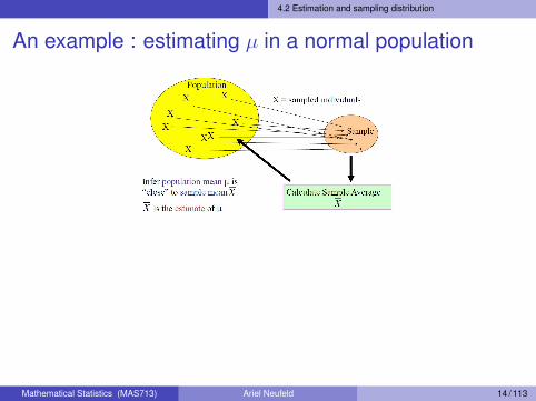
An example : estimating µ in a normal population
Mathematical Statistics (MAS713) Ariel Neufeld 14 / 113
4.2 Estimation and sampling distribution
Interval estimation : introduction
Non-formal example:1 Point estimate: the temperature today is 32o.2 Interval estimate: the temperature today is between 28o and 34o
with probability 0.95.Interval estimation gives up certainty and precision regarding the valueof the parameter, but gains confidence regarding the parameter beinginside a pre-specified interval.
Mathematical Statistics (MAS713) Ariel Neufeld 15 / 113

4.2 Estimation and sampling distribution
Interval estimation : introduction
When the estimator is normally distributed, we can be ‘reasonablyconfident’ that the true value of the parameter lies within two standarderrors of the estimate
=⇒ 68-95-99-rule - see Chapter 3.3
Mathematical Statistics (MAS713) Ariel Neufeld 16 / 113

4.2 Estimation and sampling distribution
The 68-95-99 rule for normal distributions
P(µ− σ < X < µ+ σ) ' 0.6827P(µ− 2σ < X < µ+ 2σ) ' 0.9545P(µ− 3σ < X < µ+ 3σ) ' 0.9973
Mathematical Statistics (MAS713) Ariel Neufeld 17 / 113
4.2 Estimation and sampling distribution
Interval estimation : introduction
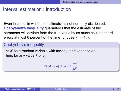
Even in cases in which the estimator is not normally distributed,Chebyshev’s inequality guarantees that the estimate of theparameter will deviate from the true value by as much as 4 standarderrors at most 6 percent of the time (choose k := 4σ).
Chebyshev’s inequality
Let X be a random variable with mean µ and variance σ2.Then, for any value k > 0,
P(|X − µ| ≥ k) ≤ σ2
k2
Mathematical Statistics (MAS713) Ariel Neufeld 18 / 113

4.2 Estimation and sampling distribution
Interval estimation : introduction
As we see, it is often easy to determine an interval of plausible valuesfor a parameter
; such observations are the basis of interval estimation
; instead of giving a point estimate θ̂, that is a single value that weknow not to be equal to θ anyway, we give
an interval in which we are very confident to find the true value
Mathematical Statistics (MAS713) Ariel Neufeld 19 / 113
4.2 Estimation and sampling distribution
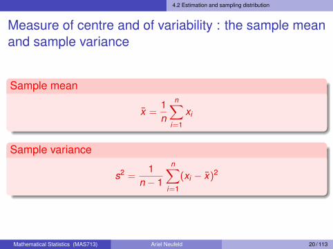
Measure of centre and of variability : the sample meanand sample variance
Sample mean
x̄ =1n
n∑i=1
xi
Sample variance
s2 =1
n − 1
n∑i=1
(xi − x̄)2
Mathematical Statistics (MAS713) Ariel Neufeld 20 / 113

4.2 Estimation and sampling distribution
Non-formal example
Mathematical Statistics (MAS713) Ariel Neufeld 21 / 113

4.2 Estimation and sampling distribution
Basic interval estimation : example
ExampleSuppose we are given a sample of size n from a population with a Normaldistribution :
X ∼ N (µ,1)
The sample mean is given by
X̄ =1n
n∑i=1
Xi
which means thatX̄ ∼ N (µ,
1√n
)
Mathematical Statistics (MAS713) Ariel Neufeld 22 / 113
4.2 Estimation and sampling distribution
Basic interval estimation : example
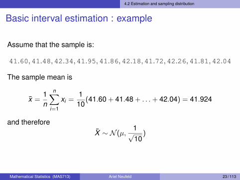
Assume that the sample is:
41.60,41.48,42.34,41.95,41.86,42.18,41.72,42.26,41.81,42.04
The sample mean is
x̄ =1n
n∑i=1
xi =1
10(41.60 + 41.48 + . . .+ 42.04) = 41.924
and thereforeX̄ ∼ N (µ,
1√10
)
Mathematical Statistics (MAS713) Ariel Neufeld 23 / 113
4.2 Estimation and sampling distribution
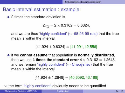
Basic interval estimation : example2 times the standard deviation is
2σX̄ = 2× 0.3162 = 0.6324,
and we are thus ‘highly confident’ (; 68-95-99 rule) that the truemean is within the interval
[41.924± 0.6324] = [41.291,42.556]
if we cannot assume that population is normally distributed,then we use 4 times the standard error 4× 0.3162 = 1.2648,and we remain ‘highly confident’ (; Chebyshev) that the truemean is within the interval
[41.924± 1.2648] = [40.6592,43.188]
; the term ‘highly confident’ obviously needs to be quantifiedMathematical Statistics (MAS713) Ariel Neufeld 24 / 113

4.2 Estimation and sampling distribution
Confidence intervals
Mathematical Statistics (MAS713) Ariel Neufeld 25 / 113
4.2 Estimation and sampling distribution
Confidence intervals
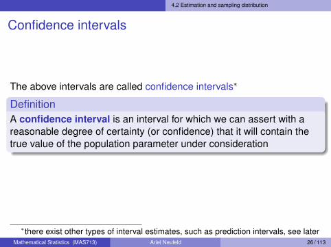
The above intervals are called confidence intervals∗
DefinitionA confidence interval is an interval for which we can assert with areasonable degree of certainty (or confidence) that it will contain thetrue value of the population parameter under consideration
∗there exist other types of interval estimates, such as prediction intervals, see laterMathematical Statistics (MAS713) Ariel Neufeld 26 / 113
4.2 Estimation and sampling distribution
Confidence intervals
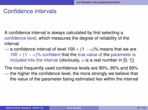
A confidence interval is always calculated by first selecting aconfidence level, which measures the degree of reliability of theinterval; a confidence interval of level 100× (1− α)% means that we are
100× (1− α)% confident that the true value of the parameter isincluded into the interval (obviously, α is a real number in [0,1])
The most frequently used confidence levels are 90%, 95% and 99%; the higher the confidence level, the more strongly we believe that
the value of the parameter being estimated lies within the interval
Mathematical Statistics (MAS713) Ariel Neufeld 27 / 113

4.2 Estimation and sampling distribution
Confidence intervals : remarks
Information about the precision of estimation is conveyed by the lengthof the interval.
a short interval implies precise estimation,a wide interval however means that there is a great deal of uncertaintyconcerning the parameter that we are estimating
Note that the higher the level of the interval, the wider it must be!
Mathematical Statistics (MAS713) Ariel Neufeld 28 / 113

4.2 Estimation and sampling distribution
Confidence intervals : remarks
FactThe 100× (1− α)% refers to the percentage of all samples of thesame size possibly drawn from the population which would produce aninterval containing the true θ
Mathematical Statistics (MAS713) Ariel Neufeld 29 / 113
4.2 Estimation and sampling distribution
Confidence intervals : remarks
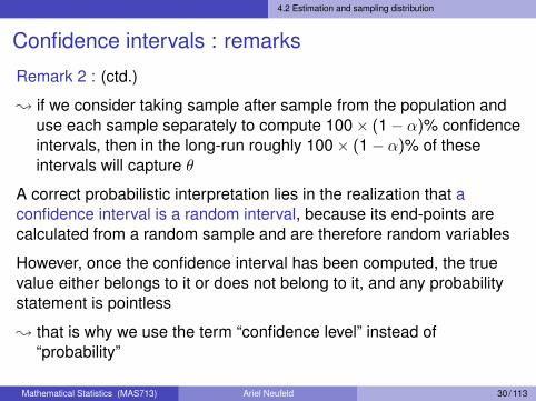
Remark 2 : (ctd.)
; if we consider taking sample after sample from the population anduse each sample separately to compute 100× (1− α)% confidenceintervals, then in the long-run roughly 100× (1− α)% of theseintervals will capture θ
A correct probabilistic interpretation lies in the realization that aconfidence interval is a random interval, because its end-points arecalculated from a random sample and are therefore random variables
However, once the confidence interval has been computed, the truevalue either belongs to it or does not belong to it, and any probabilitystatement is pointless
; that is why we use the term “confidence level” instead of“probability”
Mathematical Statistics (MAS713) Ariel Neufeld 30 / 113

4.2 Estimation and sampling distribution
Confidence intervals : remarksAs an illustration, we successively computed 95%-confidence intervalsfor µ for 100 random samples of size 100 independently drawn from aN (0,1) population
0 20 40 60 80 100
−0.
4−
0.2
0.0
0.2
0.4
sample number
; 96 intervals out of 100 contain the true value µ = 0
Obviously, in practice we do not know the true value of µ, and wecannot tell whether the interval we have computed is one of the ‘good’95% intervals or one of the ‘bad’ 5% intervals
Mathematical Statistics (MAS713) Ariel Neufeld 31 / 113
4.2 CI on the mean of a normal distribution, known σ2
Confidence interval on the mean of a normal distribution, varianceknown
Mathematical Statistics (MAS713) Ariel Neufeld 32 / 113

4.2 CI on the mean of a normal distribution, known σ2
Confidence interval on the mean of a normaldistribution, variance known
The basic ideas for building confidence intervals are most easilyunderstood by first considering a simple situation :
Suppose we have a normal population withunknown mean µ andknown variance σ2
Note that this is somewhat unrealistic, as typically both the mean andthe variance are unknown
; we will address more general situations later
Mathematical Statistics (MAS713) Ariel Neufeld 33 / 113

4.2 CI on the mean of a normal distribution, known σ2
Confidence interval on the mean of a normaldistribution, variance known
We have thus a random sample X1,X2, . . . ,Xn, such that, for all i ,
Xi ∼ N (µ, σ),
with µ unknown and σ a known constant
Mathematical Statistics (MAS713) Ariel Neufeld 34 / 113

4.2 CI on the mean of a normal distribution, known σ2
Confidence interval on the mean of a normaldistribution, variance known
Suppose we desire a confidence interval for µ of level 100× (1− α)%
From our random sample, this can be regarded as a ‘random interval’,say [L,U], where L and U are statistics, and such that
P(L ≤ µ ≤ U) = 1− α
Mathematical Statistics (MAS713) Ariel Neufeld 35 / 113

4.2 CI on the mean of a normal distribution, known σ2
Confidence interval on the mean of a normaldistribution, variance known
In that situation, we know that, for any integer n ≥ 1,
X̄ =1n
n∑i=1
Xi ∼ N(µ,
σ√n
)We may standardise this normally distributed random variable :
Z =X̄ − µσ/√
n=√
nX̄ − µσ∼ N (0,1)
Mathematical Statistics (MAS713) Ariel Neufeld 36 / 113

4.2 CI on the mean of a normal distribution, known σ2
Confidence interval on the mean of a normaldistribution, variance known
In our situation, becauseZ ∼ N (0,1), we may write
P(−z1−α/2 ≤ Z ≤ z1−α/2) = 1− α
where z1−α/2 is the quantile of level1− α/2 of the standard normaldistribution,
x
φ(x)
− z1−α 2 0 z1−α 2
0.0
0.1
0.2
0.3
0.4
α 2α 2
1 − α
that is,
P(−z1−α/2 ≤
√n
X̄ − µσ≤ z1−α/2
)= 1− α
Mathematical Statistics (MAS713) Ariel Neufeld 37 / 113

4.2 CI on the mean of a normal distribution, known σ2
Confidence interval on the mean of a normaldistribution, variance known
Hence,
P(
X̄ − z1−α/2σ√n≤ µ ≤ X̄ + z1−α/2
σ√n
)= 1− α
; we have found L and U, two statistics (random variables dependingon the sample) such that
P(L ≤ µ ≤ U) = 1− α
; L and U will yield the bounds of the confidence interval !
Mathematical Statistics (MAS713) Ariel Neufeld 38 / 113
4.2 CI on the mean of a normal distribution, known σ2
Confidence interval on the mean of a normaldistribution, variance known
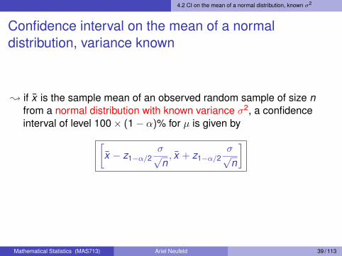
; if x̄ is the sample mean of an observed random sample of size nfrom a normal distribution with known variance σ2, a confidenceinterval of level 100× (1− α)% for µ is given by[
x̄ − z1−α/2σ√n, x̄ + z1−α/2
σ√n
]
Mathematical Statistics (MAS713) Ariel Neufeld 39 / 113

4.2 CI on the mean of a normal distribution, known σ2
Confidence interval on the mean of a normaldistribution, variance knownFrom Chapter 3.3: z0.95 = 1.645, z0.975 = 1.96 and z0.995 = 2.575
; a confidence interval for µ of level 90% is[x̄ − 1.645× σ√
n , x̄ + 1.645× σ√n
]; a confidence interval for µ of level 95% is[
x̄ − 1.96× σ√n , x̄ + 1.96× σ√
n
]; a confidence interval for µ of level 99% is[
x̄ − 2.575× σ√n , x̄ + 2.575× σ√
n
]We see that the respective lengths of these intervals are
3.29σ√n, 3.92
σ√n
and 5.15σ√n
Mathematical Statistics (MAS713) Ariel Neufeld 40 / 113
4.2 CI on the mean of a normal distribution, known σ2
Confidence interval on the mean of a normaldistribution, variance known : choice of sample size
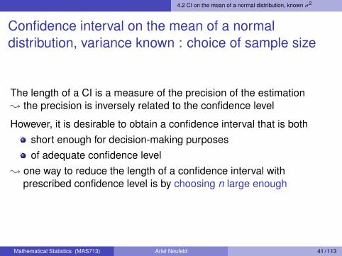
The length of a CI is a measure of the precision of the estimation; the precision is inversely related to the confidence level
However, it is desirable to obtain a confidence interval that is bothshort enough for decision-making purposesof adequate confidence level
; one way to reduce the length of a confidence interval withprescribed confidence level is by choosing n large enough
Mathematical Statistics (MAS713) Ariel Neufeld 41 / 113
4.2 CI on the mean of a normal distribution, known σ2
Confidence interval on the mean of a normaldistribution, variance known : choice of sample size
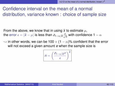
From the above, we know that in using x̄ to estimate µ,the error e = |x̄ − µ| is less than z1−α/2
σ√n with confidence 1− α
; in other words, we can be 100× (1− α)% confident that the errorwill not exceed a given amount e when the sample size is
n =
(z1−α/2σ
e
)2
Mathematical Statistics (MAS713) Ariel Neufeld 42 / 113

4.2 CI on the mean of a normal distribution, known σ2
Confidence interval on the mean of a normaldistribution, variance known : example
ExampleTen measurements of temperature are as follows :
64.1,64.7,64.5,64.6,64.5,64.3,64.6,64.8,64.2,64.3
Assume that temperature is normally distributed with σ = 1c.a) Find a 95% CI for µ, the mean temperature
An elementary computation yields x̄ = 64.46.With n = 10, σ = 1 and α = 0.05, direct application of the previous resultsgives a 95% CI as follows :[
x̄ − zα/2σ√n, x̄ + zα/2
σ√n
]=
[64.46− 1.96× 1√
10,64.46 + 1.96× 1√
10
]= [63.84,65.08]
Mathematical Statistics (MAS713) Ariel Neufeld 43 / 113

4.2 CI on the mean of a normal distribution, known σ2
Confidence interval on the mean of a normaldistribution, variance known : example
Example (ctd.)b) Determine how many measurements we should take to ensure that the95% CI on the mean temperature µ has a length of at most 1,
The length of the CI in part a) is 1.24.If we desire a higher precision, namely an confidence interval length of 1,then we need more than 10 observations
The bound on error estimation e is one-half of the length of the CI, thus useexpression on Slide 34 with e = 0.5, σ = 1 and α = 0.05 :
n =
(zα/2σ
e
)2
=
(1.96× 1
0.5
)2
= 15.37
; as n must be an integer, the required sample size is 16
Mathematical Statistics (MAS713) Ariel Neufeld 44 / 113
4.2 CI on the mean of a normal distribution, known σ2
Confidence interval on the mean of a normaldistribution, variance known : remarks
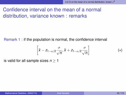
Remark 1 : if the population is normal, the confidence interval[x̄ − z1−α/2
σ√n, x̄ + z1−α/2
σ√n
](?)
is valid for all sample sizes n ≥ 1
Mathematical Statistics (MAS713) Ariel Neufeld 45 / 113
4.2 CI on the mean of a normal distribution, known σ2
Confidence interval on the mean of a normaldistribution, variance known : remarks
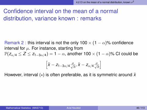
Remark 2 : this interval is not the only 100× (1− α)% confidenceinterval for µ. For instance, starting fromP(zα/4 ≤ Z ≤ z1−3α/4) = 1− α, another 100× (1− α)% CI could be[
x̄ − z1−3α/4σ√n , x̄ − zα/4
σ√n
]However, interval (?) is often preferable, as it is symmetric around x̄
Mathematical Statistics (MAS713) Ariel Neufeld 46 / 113

4.2 CI on the mean of a normal distribution, known σ2
Confidence interval on the mean of a normaldistribution, variance known : remarks
Remark 3 : in the same spirit, we haveP(Z ≤ z1−α) = P(−z1−α ≤ Z ) = 1− α
Hence, ]−∞, x̄ + z1−ασ√n ] and [x̄ − z1−α
σ√n ,+∞[ are also
100× (1− α)% CI for µ
; these are called one-sided confidence intervals,as opposed to (?) (two-sided CI) ; Slide 45.
Mathematical Statistics (MAS713) Ariel Neufeld 47 / 113

4.3 CI on the mean of a normal distribution, unknown σ2
Confidence interval on the mean of a normal distribution, varianceunknown
Mathematical Statistics (MAS713) Ariel Neufeld 48 / 113

4.3 CI on the mean of a normal distribution, unknown σ2
Confidence interval on the mean of a normaldistribution, variance unknown
Suppose now that the population variance σ2 is not known(meaning that now bothbµ and σ2 are unknown).
; we can no longer make practical use of the core result
Z =√
n X̄−µσ ∼ N (0,1)
Mathematical Statistics (MAS713) Ariel Neufeld 49 / 113
4.3 CI on the mean of a normal distribution, unknown σ2
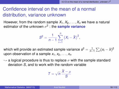
Confidence interval on the mean of a normaldistribution, variance unknownHowever, from the random sample X1,X2, . . . ,Xn we have a naturalestimator of the unknown σ2 : the sample variance
S2 =1
n − 1
n∑i=1
(Xi − X̄
)2,
which will provide an estimated sample variance s2 = 1n−1
∑i(xi − x̄)2
upon observation of a sample x1, x2, . . . , xn
; a logical procedure is thus to replace σ with the sample standarddeviation S, and to work with the random variable
T =√
nX̄ − µ
S
Mathematical Statistics (MAS713) Ariel Neufeld 50 / 113

4.3 CI on the mean of a normal distribution, unknown σ2
Confidence interval on the mean of a normaldistribution, variance unknown
The fact is that, if Z was a standardised version of a normal r.v. X̄ andwas therefore normally distributed, T is now a ratio of two randomvariables (X̄ − µ and S)
; T is not N (0,1)-distributed !
Mathematical Statistics (MAS713) Ariel Neufeld 51 / 113

4.3 CI on the mean of a normal distribution, unknown σ2
Confidence interval on the mean of a normaldistribution, variance unknown
Indeed, T cannot have the same distribution as Z , as the estimation ofthe constant σ by a random variable S introduces some extra variability
; the random variable T varies much more in value from sample tosample than does Z
It turns out that, for n ≥ 2,
T follows the so-called t-distribution with n− 1 degrees of freedom
Mathematical Statistics (MAS713) Ariel Neufeld 52 / 113

4.4. The Student’s t-distribution
The Student’s t-distribution
Mathematical Statistics (MAS713) Ariel Neufeld 53 / 113

4.4. The Student’s t-distribution
The Student’s t-distribution
The first who realized that replacing σ with an estimation effectivelyaffected the distribution of Z was William Gosset (1876-1937), a Britishchemist and mathematician who, worked at the Guinness Brewery inDublin
Another researcher at Guinness had previously published a papercontaining trade secrets of the Guinness brewery, so that Guinnessprohibited its employees from publishing any papers regardless of thecontained information
; Gosset used the pseudonym Student for his publications to avoidtheir detection by his employer
Thus his most famous achievement is now referred to as Student’st-distribution, which might otherwise have been Gosset’s t-distribution
Mathematical Statistics (MAS713) Ariel Neufeld 54 / 113

4.4. The Student’s t-distribution
The Student’s t-distributionA random variable, say T , is said to follow the Student’s t-distributionwith ν degrees of freedom, i.e.
T ∼ tν
if its probability density function is given by
f (t) =Γ(ν+1
2
)√νπΓ
(ν2
) (1 +t2
ν
)− ν+12
; ST = R
for some integer ν
Note : the Gamma function is given by
Γ(y) =
∫ +∞
0xy−1e−x dx , for y > 0
It can be shown that Γ(y) = (y − 1)× Γ(y − 1), so that, if y is a positiveinteger n, Γ(n) = (n − 1)!
There is no simple expression for the Student’s t-cdfMathematical Statistics (MAS713) Ariel Neufeld 55 / 113

4.4. The Student’s t-distribution
The Student’s t-distributionStudent’s t distribution with 1 degree of freedom
−4 −2 0 2 4
0.0
0.2
0.4
0.6
0.8
1.0
t
F(t)
−4 −2 0 2 4
0.0
0.1
0.2
0.3
0.4
t
f(t)
cdf F (t) pdf f (t) = F ′(t)
Mathematical Statistics (MAS713) Ariel Neufeld 56 / 113
4.4. The Student’s t-distribution
The Student’s t-distribution
−4 −2 0 2 4
0.0
0.1
0.2
0.3
0.4
Student's distributions and standard normal
t
f(t)
Mathematical Statistics (MAS713) Ariel Neufeld 57 / 113

4.4. The Student’s t-distribution
The Student’s t-distribution
−4 −2 0 2 4
0.0
0.1
0.2
0.3
0.4
Student's distributions and standard normal
t
f(t)
Mathematical Statistics (MAS713) Ariel Neufeld 57 / 113

4.4. The Student’s t-distribution
The Student’s t-distribution
−4 −2 0 2 4
0.0
0.1
0.2
0.3
0.4
Student's distributions and standard normal
t
f(t)
Mathematical Statistics (MAS713) Ariel Neufeld 57 / 113

4.4. The Student’s t-distribution
The Student’s t-distribution
−4 −2 0 2 4
0.0
0.1
0.2
0.3
0.4
Student's distributions and standard normal
t
f(t)
Mathematical Statistics (MAS713) Ariel Neufeld 57 / 113

4.4. The Student’s t-distribution
The Student’s t-distribution
−4 −2 0 2 4
0.0
0.1
0.2
0.3
0.4
Student's distributions and standard normal
t
f(t)
t1t2t5t10
t50
N(0,1)
t1t2t5t10
t50
N(0,1)
Mathematical Statistics (MAS713) Ariel Neufeld 57 / 113

4.4. The Student’s t-distribution
The Student’s t-distribution
Mean and variance of the tν-distributionIf T ∼ tν , E(T ) = 0 and Var(T ) =
ν
ν − 2
Mathematical Statistics (MAS713) Ariel Neufeld 58 / 113

4.4. The Student’s t-distribution
The Student’s t-distribution
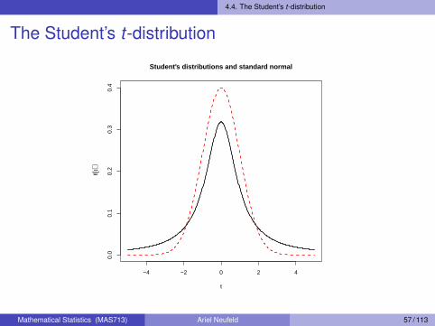
The Student’s t distribution is similar to the standard normaldistribution in that both densities are symmetric and unimodal, and themaximum value is reached at t = 0
However, the Student’s t distribution has heavier tails than the normal
; there is more probability to find the random variable T ‘far away’from 0 than there is for Z
This is more marked for small values of ν
As the number ν of degrees of freedom increases, tν-distributions lookmore and more like the standard normal distribution
In fact, it can be shown that the Student’s t distribution with ν degreesof freedom approaches the standard normal distribution as ν →∞
Mathematical Statistics (MAS713) Ariel Neufeld 59 / 113

4.4. The Student’s t-distribution
The Student’s t-distribution : quantiles
Similarly to what we did for the Normal distribution, we can define thequantiles of any Student’s t-distribution
Mathematical Statistics (MAS713) Ariel Neufeld 60 / 113
4.4. The Student’s t-distribution
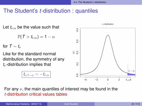
The Student’s t-distribution : quantiles
Let tν;α be the value such that
P(T > tν;α) = 1− α
for T ∼ tν
Like for the standard normaldistribution, the symmetry of anytν-distribution implies that
tν;1−α = −tν;α
−4 −2 0 2 40.
00.
10.
20.
30.
4
tν−distribution
t
f(t)
tν, α
1 − α
For any ν, the main quantiles of interest may be found in thet-distribution critical values tables
Mathematical Statistics (MAS713) Ariel Neufeld 61 / 113

4.4. The Student’s t-distribution
t-distribution critical values tablest Table
cum. prob t .50 t .75 t .80 t .85 t .90 t .95 t .975 t .99 t .995 t .999 t .9995
one-tail 0.50 0.25 0.20 0.15 0.10 0.05 0.025 0.01 0.005 0.001 0.0005two-tails 1.00 0.50 0.40 0.30 0.20 0.10 0.05 0.02 0.01 0.002 0.001
df1 0.000 1.000 1.376 1.963 3.078 6.314 12.71 31.82 63.66 318.31 636.622 0.000 0.816 1.061 1.386 1.886 2.920 4.303 6.965 9.925 22.327 31.5993 0.000 0.765 0.978 1.250 1.638 2.353 3.182 4.541 5.841 10.215 12.9244 0.000 0.741 0.941 1.190 1.533 2.132 2.776 3.747 4.604 7.173 8.6105 0.000 0.727 0.920 1.156 1.476 2.015 2.571 3.365 4.032 5.893 6.8696 0.000 0.718 0.906 1.134 1.440 1.943 2.447 3.143 3.707 5.208 5.9597 0.000 0.711 0.896 1.119 1.415 1.895 2.365 2.998 3.499 4.785 5.4088 0.000 0.706 0.889 1.108 1.397 1.860 2.306 2.896 3.355 4.501 5.0419 0.000 0.703 0.883 1.100 1.383 1.833 2.262 2.821 3.250 4.297 4.781
10 0.000 0.700 0.879 1.093 1.372 1.812 2.228 2.764 3.169 4.144 4.58711 0.000 0.697 0.876 1.088 1.363 1.796 2.201 2.718 3.106 4.025 4.43712 0.000 0.695 0.873 1.083 1.356 1.782 2.179 2.681 3.055 3.930 4.31813 0.000 0.694 0.870 1.079 1.350 1.771 2.160 2.650 3.012 3.852 4.22114 0.000 0.692 0.868 1.076 1.345 1.761 2.145 2.624 2.977 3.787 4.14015 0.000 0.691 0.866 1.074 1.341 1.753 2.131 2.602 2.947 3.733 4.07316 0.000 0.690 0.865 1.071 1.337 1.746 2.120 2.583 2.921 3.686 4.01517 0.000 0.689 0.863 1.069 1.333 1.740 2.110 2.567 2.898 3.646 3.96518 0.000 0.688 0.862 1.067 1.330 1.734 2.101 2.552 2.878 3.610 3.92219 0.000 0.688 0.861 1.066 1.328 1.729 2.093 2.539 2.861 3.579 3.88320 0.000 0.687 0.860 1.064 1.325 1.725 2.086 2.528 2.845 3.552 3.85021 0.000 0.686 0.859 1.063 1.323 1.721 2.080 2.518 2.831 3.527 3.81922 0.000 0.686 0.858 1.061 1.321 1.717 2.074 2.508 2.819 3.505 3.79223 0.000 0.685 0.858 1.060 1.319 1.714 2.069 2.500 2.807 3.485 3.76824 0.000 0.685 0.857 1.059 1.318 1.711 2.064 2.492 2.797 3.467 3.74525 0.000 0.684 0.856 1.058 1.316 1.708 2.060 2.485 2.787 3.450 3.72526 0.000 0.684 0.856 1.058 1.315 1.706 2.056 2.479 2.779 3.435 3.70727 0.000 0.684 0.855 1.057 1.314 1.703 2.052 2.473 2.771 3.421 3.69028 0.000 0.683 0.855 1.056 1.313 1.701 2.048 2.467 2.763 3.408 3.67429 0.000 0.683 0.854 1.055 1.311 1.699 2.045 2.462 2.756 3.396 3.65930 0.000 0.683 0.854 1.055 1.310 1.697 2.042 2.457 2.750 3.385 3.64640 0.000 0.681 0.851 1.050 1.303 1.684 2.021 2.423 2.704 3.307 3.55160 0.000 0.679 0.848 1.045 1.296 1.671 2.000 2.390 2.660 3.232 3.46080 0.000 0.678 0.846 1.043 1.292 1.664 1.990 2.374 2.639 3.195 3.416
100 0.000 0.677 0.845 1.042 1.290 1.660 1.984 2.364 2.626 3.174 3.3901000 0.000 0.675 0.842 1.037 1.282 1.646 1.962 2.330 2.581 3.098 3.300
z 0.000 0.674 0.842 1.036 1.282 1.645 1.960 2.326 2.576 3.090 3.2910% 50% 60% 70% 80% 90% 95% 98% 99% 99.8% 99.9%
Confidence Level
t-table.xls 7/14/2007
Mathematical Statistics (MAS713) Ariel Neufeld 62 / 113
4.4. The Student’s t-distribution
Confidence interval on the mean of a normaldistribution, variance unknown
So we have, for any n ≥ 2,
T =√
nX̄ − µ
S∼ tn−1
Note : the number of degrees of freedom for the t-distribution is thenumber of degrees of freedom associated with the estimated varianceS2
Mathematical Statistics (MAS713) Ariel Neufeld 63 / 113
4.4. The Student’s t-distribution
Confidence interval on the mean of a normaldistribution, variance unknown
It is now easy to find a 100× (1− α)% confidence interval for µ byproceeding essentially as we did when σ2 was known
We may write
P(−tn−1;1−α/2 ≤
√n
X̄ − µS
≤ tn−1;1−α/2
)= 1− α
or
P(
X̄ − tn−1;1−α/2S√n≤ µ ≤ X̄ + tn−1;1−α/2
S√n
)= 1− α
Mathematical Statistics (MAS713) Ariel Neufeld 64 / 113
4.4. The Student’s t-distribution
Confidence interval on the mean of a normaldistribution, variance unknown
; if x̄ and s are the sample mean and sample standard deviation ofan observed random sample of size n from a normal distribution, aconfidence interval of level 100× (1− α)% for µ is given by[
x̄ − tn−1;1−α/2s√n, x̄ + tn−1;1−α/2
s√n
]This confidence interval is sometimes called t-confidence interval, asopposed to (?) (z-confidence interval)
Mathematical Statistics (MAS713) Ariel Neufeld 65 / 113

4.4. The Student’s t-distribution
Confidence interval on the mean of a normaldistribution, variance unknown
Because tn−1 has heavier tails than N (0,1), tn−1;1−α/2 > z1−α/2
; this renders the extra variability introduced by the estimation of σ(less accuracy)
Note : One can also define one-sided 100× (1− α)% t-confidenceintervals
]−∞, x̄ + tn−1;1−αs√n ] and [x̄ − tn−1;1−α
s√n ,+∞[
Mathematical Statistics (MAS713) Ariel Neufeld 66 / 113

4.4. The Student’s t-distribution
Confidence interval on the mean of a normaldistribution, variance unknown : example
ExampleA sample with 22 measurements of the temperature is as follows :
7.6, 8.1, 11.7, 14.3, 14.3, 14.1, 8.3, 12.3, 15.9, 16.4,11.3, 12.0, 12.9, 15.0, 13.2, 14.6, 13.5, 10.4, 13.8,
15.6, 12.2, 11.2
Construct a 99% confidence interval for the mean temperature
Elementary computations give
x̄ = 12.67 and s = 2.47
Mathematical Statistics (MAS713) Ariel Neufeld 67 / 113

4.4. The Student’s t-distribution
Confidence interval on the mean of a normaldistribution, variance unknown : example
The quantile plot below provides goodsupport for the assumption that thepopulation is normally distributed
●
●
●
●
●
●
●
●
●
●
●
●
●
●
●
●
●
●
●
●
●
●
8 10 12 14 16
−2
−1
01
2
Normal Q−Q Plot
Sample Quantiles
The
oret
ical
Qua
ntile
s
Since n = 22, we have n − 1 = 21 degrees of freedom for t . In the table, wefind t21;0.995 = 2.831. The resulting CI is[
x̄ − tn−1;1−α/2s√n, x̄ + tn−1;1−α/2
s√n
]=
[12.67± 2.831× 2.47√
22
]= [11.18,14.16]
; we are 99% confident that the mean temperature lies between 11.18 and14.16 degress.
Mathematical Statistics (MAS713) Ariel Neufeld 68 / 113

4.5. General method to derive a confidence interval
General method to derive aconfidence interval
Mathematical Statistics (MAS713) Ariel Neufeld 69 / 113

4.5. General method to derive a confidence interval
General method to derive a confidence interval
By looking at the previous two situations (CI for µ in a normalpopulation, σ2 known or unknown), it is now easy to give a generalmethod for finding a confidence interval for any unknown parameter θ
Mathematical Statistics (MAS713) Ariel Neufeld 70 / 113
4.5. General method to derive a confidence interval
General method to derive a confidence interval
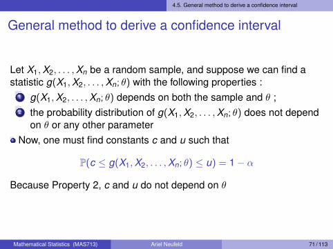
Let X1,X2, . . . ,Xn be a random sample, and suppose we can find astatistic g(X1,X2, . . . ,Xn; θ) with the following properties :
1 g(X1,X2, . . . ,Xn; θ) depends on both the sample and θ ;2 the probability distribution of g(X1,X2, . . . ,Xn; θ) does not depend
on θ or any other parameterNow, one must find constants c and u such that
P(c ≤ g(X1,X2, . . . ,Xn; θ) ≤ u) = 1− α
Because Property 2, c and u do not depend on θ
Mathematical Statistics (MAS713) Ariel Neufeld 71 / 113
4.5. General method to derive a confidence interval
General method to derive a confidence interval
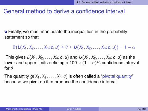
Finally, we must manipulate the inequalities in the probabilitystatement so that
P(L(X1,X2, . . . ,Xn; c,u) ≤ θ ≤ U(X1,X2, . . . ,Xn; c,u)) = 1− α
This gives L(X1,X2, . . . ,Xn; c,u) and U(X1,X2, . . . ,Xn; c,u) as thelower and upper limits defining a 100× (1− α)% confidence intervalfor θ
The quantity g(X1,X2, . . . ,Xn; θ) is often called a “pivotal quantity”because we pivot on it to produce the confidence interval
Mathematical Statistics (MAS713) Ariel Neufeld 72 / 113

4.5. General method to derive a confidence interval
General method to derive a confidence interval
Example:
θ = µ in a normal population with known variance, then
=⇒ g(X1,X2, . . . ,Xn; θ) =√
n X̄−µσ ∼ N (0,1)
We hace c = −z1−α/2 and u = z1−α/2
The statistics L and U areL(X1,X2, . . . ,Xn; c,u) = X̄ − z1−α/2
σ√n ,
U(X1,X2, . . . ,Xn; c,u) = X̄ + z1−α/2σ√n
Mathematical Statistics (MAS713) Ariel Neufeld 73 / 113
4.6. Central Limit Theorem
Central Limit Theorem
Mathematical Statistics (MAS713) Ariel Neufeld 74 / 113

4.6. Central Limit Theorem
Introduction
So far we have assumed that the population distribution is normal. Inthat situation, we have
Z =√
nX̄ − µσ∼ N (0,1) and T =
√n
X̄ − µS
∼ tn−1
where X̄ is the sample mean and S2 is the sample variance of arandom sample of size n
These sampling distributions are the cornerstone when derivingconfidence intervals for µ, and directly follow from Xi ∼ N (µ, σ)
Mathematical Statistics (MAS713) Ariel Neufeld 75 / 113

4.6. Central Limit Theorem
Introduction
A natural question is now :
What if the population is not normal?
; surprisingly enough, the above results still hold most of the time, atleast approximately, due to the so-called
Central Limit Theorem
Mathematical Statistics (MAS713) Ariel Neufeld 76 / 113

4.6. Central Limit Theorem
The Central Limit Theorem
The Central Limit Theorem (CLT) is certainly one of the mostremarkable results in probability (“the unofficial sovereign of probabilitytheory”). Loosely speaking, it asserts that
the sum of a large number of independent random variables has adistribution that is approximately normal
It was first postulated by Abraham de Moivre who used the bell-shapedcurve to approximate the distribution of the number of heads resultingfrom many tosses of a fair coin
Mathematical Statistics (MAS713) Ariel Neufeld 77 / 113

4.6. Central Limit Theorem
The Central Limit Theorem
However, this received little attention until the French mathematicianPierre-Simon Laplace (1749-1827) rescued it from obscurity in hismonumental work “Théorie Analytique des Probabilités”, which waspublished in 1812
But it was not before 1901 that it was defined in general terms andformally proved by the Russian mathematician Aleksandr Lyapunov(1857-1918)
Mathematical Statistics (MAS713) Ariel Neufeld 78 / 113

4.6. Central Limit Theorem
The Central Limit Theorem
Central Limit TheoremIf X1,X2, . . . ,Xn is a random sample (meaning i.i.d.) taken from apopulation with finite mean µ and finite variance σ2,and if X̄ denotes the sample mean, then the limiting distribution of
1√n
∑ni=1 Xi − nµ
σ=√
nX̄ − µσ
as n→∞, is the standard normal distribution
Mathematical Statistics (MAS713) Ariel Neufeld 79 / 113

4.6. Central Limit Theorem
The Central Limit Theorem
When Xi ∼ N (µ, σ),√
n X̄−µσ ∼ N (0,1) for all n
What the CLT states is that, when Xi ’s are not normal,√n X̄−µ
σ ∼ N (0,1) when n is infinitely large
; the standard normal distribution provides a reasonableapproximation to the distribution of
√n X̄−µ
σ when “n is large”
Mathematical Statistics (MAS713) Ariel Neufeld 80 / 113

4.6. Central Limit Theorem
The Central Limit Theorem
The power of the CLT is that it holds true for any populationdistribution, discrete or continuous ! For instance,
Xi ∼ Exp(λ) (µ =1λ, σ =
1λ
) =⇒√
nX̄ − 1/λ
1/λa∼ N (0,1)
Xi ∼ U[a,b] (µ =a + b
2, σ =
b − a√12
) =⇒√
nX̄ − a+b
2b−a√
12
a∼ N (0,1)
Xi ∼ Bern(π) (µ = π, σ =√π(1− π)) =⇒
√n
X̄ − π√π(1− π)
a∼ N (0,1)
Note : a∼ is for ‘approximately follows’(or ‘asymptotically (n→∞) follows’)
Mathematical Statistics (MAS713) Ariel Neufeld 81 / 113

4.6. Central Limit Theorem
The Central Limit Theorem
Facts :the larger n, the better the normal approximationthe closer the population is to being normal, the more rapidly thedistribution of
√n X̄−µ
σ approaches normality as n gets large
Mathematical Statistics (MAS713) Ariel Neufeld 82 / 113
4.6. Central Limit Theorem
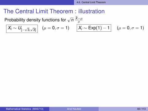
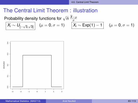
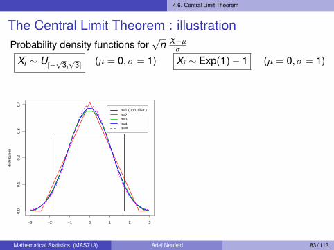
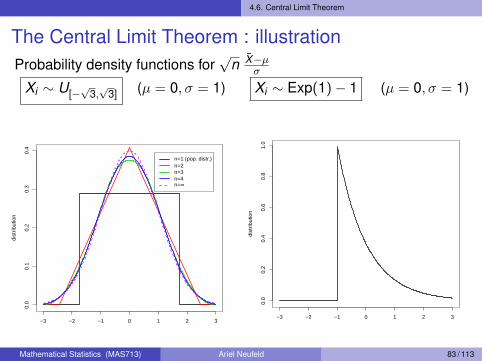
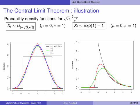
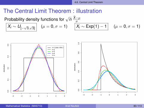
The Central Limit Theorem : illustrationProbability density functions for
√n X̄−µ
σ
Xi ∼ U[−√
3,√
3] (µ = 0, σ = 1) Xi ∼ Exp(1)− 1 (µ = 0, σ = 1)
Mathematical Statistics (MAS713) Ariel Neufeld 83 / 113
4.6. Central Limit Theorem
The Central Limit Theorem : illustrationProbability density functions for
√n X̄−µ
σ
Xi ∼ U[−√
3,√
3] (µ = 0, σ = 1)
−3 −2 −1 0 1 2 3
0.0
0.1
0.2
0.3
0.4
dist
ribut
ion
Xi ∼ Exp(1)− 1 (µ = 0, σ = 1)
Mathematical Statistics (MAS713) Ariel Neufeld 83 / 113

4.6. Central Limit Theorem
The Central Limit Theorem : illustrationProbability density functions for
√n X̄−µ
σ
Xi ∼ U[−√
3,√
3] (µ = 0, σ = 1)
−3 −2 −1 0 1 2 3
0.0
0.1
0.2
0.3
0.4
dist
ribut
ion
Xi ∼ Exp(1)− 1 (µ = 0, σ = 1)
Mathematical Statistics (MAS713) Ariel Neufeld 83 / 113

4.6. Central Limit Theorem
The Central Limit Theorem : illustrationProbability density functions for
√n X̄−µ
σ
Xi ∼ U[−√
3,√
3] (µ = 0, σ = 1)
−3 −2 −1 0 1 2 3
0.0
0.1
0.2
0.3
0.4
dist
ribut
ion
Xi ∼ Exp(1)− 1 (µ = 0, σ = 1)
Mathematical Statistics (MAS713) Ariel Neufeld 83 / 113

4.6. Central Limit Theorem
The Central Limit Theorem : illustrationProbability density functions for
√n X̄−µ
σ
Xi ∼ U[−√
3,√
3] (µ = 0, σ = 1)
−3 −2 −1 0 1 2 3
0.0
0.1
0.2
0.3
0.4
dist
ribut
ion
Xi ∼ Exp(1)− 1 (µ = 0, σ = 1)
Mathematical Statistics (MAS713) Ariel Neufeld 83 / 113
4.6. Central Limit Theorem
The Central Limit Theorem : illustrationProbability density functions for
√n X̄−µ
σ
Xi ∼ U[−√
3,√
3] (µ = 0, σ = 1)
−3 −2 −1 0 1 2 3
0.0
0.1
0.2
0.3
0.4
dist
ribut
ion
n=1 (pop. distr.)n=2n=3n=4n=∞
Xi ∼ Exp(1)− 1 (µ = 0, σ = 1)
−3 −2 −1 0 1 2 3
0.0
0.2
0.4
0.6
0.8
1.0
dist
ribut
ion
Mathematical Statistics (MAS713) Ariel Neufeld 83 / 113

4.6. Central Limit Theorem
The Central Limit Theorem : illustrationProbability density functions for
√n X̄−µ
σ
Xi ∼ U[−√
3,√
3] (µ = 0, σ = 1)
−3 −2 −1 0 1 2 3
0.0
0.1
0.2
0.3
0.4
dist
ribut
ion
n=1 (pop. distr.)n=2n=3n=4n=∞
Xi ∼ Exp(1)− 1 (µ = 0, σ = 1)
−3 −2 −1 0 1 2 3
0.0
0.2
0.4
0.6
0.8
1.0
dist
ribut
ion
n=1 (pop. distr.)n=2n=6n=25n=50n=∞
Mathematical Statistics (MAS713) Ariel Neufeld 83 / 113

4.6. Central Limit Theorem
The Central Limit Theorem : illustrationProbability mass functions for
∑ni=1 Xi , Xi ∼ Bern(π)
π = 0.5 :
0 1 2 3 4 5
0.05
0.10
0.15
0.20
0.25
0.30
n = 5
x
p X(x
)
10 15 20 25 30 35 40
0.00
0.02
0.04
0.06
0.08
0.10
n = 50
x
p X(x
)
30 40 50 60 70
0.00
0.02
0.04
0.06
0.08
n = 100
x
p X(x
)
200 220 240 260 280 300
0.00
00.
005
0.01
00.
015
0.02
00.
025
0.03
00.
035
n = 500
x
p X(x
)
π = 0.1 :
0 1 2 3 4 5
0.0
0.1
0.2
0.3
0.4
0.5
0.6
n = 5
x
p X(x
)
0 5 10 15
0.00
0.05
0.10
0.15
n = 50
x
p X(x
)
0 5 10 15 20 25
0.00
0.02
0.04
0.06
0.08
0.10
0.12
n = 100
x
p X(x
)
0 20 40 60 80 100
0.00
0.01
0.02
0.03
0.04
0.05
0.06
n = 500
x
p X(x
)
Mathematical Statistics (MAS713) Ariel Neufeld 84 / 113

4.6. Central Limit Theorem
The Central Limit Theorem : further illustration
Matlab example
Mathematical Statistics (MAS713) Ariel Neufeld 85 / 113

4.6. Central Limit Theorem
The Central Limit Theorem : remarks
Remark 1 :
The Central Limit Theorem not only provides a simple method forcomputing approximate probabilities for sums or averages ofindependent random variables
It also helps explain why so many natural populations exhibit abell-shaped (i.e., normal) distribution curve :
indeed, as long as the behaviour of the variable of interest is dictatedby a large number of independent contributions, it should be (at leastapproximately) normally distributed
Mathematical Statistics (MAS713) Ariel Neufeld 86 / 113
4.6. Central Limit Theorem
The Central Limit Theorem : remarks
For instance, a person’s height is the result of many independentfactors, both genetic and environmental. Each of these factors canincrease or decrease a person’s height, just as each ball in Galton’sboard can bounce to the right or the left. The Central Limit Theoremguarantees that the sum of these contributions has approximately anormal distribution
Mathematical Statistics (MAS713) Ariel Neufeld 87 / 113

4.6. Central Limit Theorem
The Central Limit Theorem : remarksRemark 2 :
a natural question is ‘how large n needs to be’ for the normalapproximation to be valid
; that depends on the population distribution !
A general rule-of-thumb is that one can be confident of the normalapproximation whenever the sample size n is at least 30
n ≥ 30
Note that, in favourable cases (population distribution not severelynon-normal), the normal approximation will be satisfactory for muchsmaller sample sizes (like n = 5 in the uniform case, for instance)
The rule “n ≥ 30” just guarantees that the normal distribution providesa good approximation to the sampling distribution of X̄ regardless ofthe shape of the population
Mathematical Statistics (MAS713) Ariel Neufeld 88 / 113

4.7 Confidence interval on the mean of an arbitrary population
Confidence interval on the mean ofan arbitrary population
Mathematical Statistics (MAS713) Ariel Neufeld 89 / 113
4.7 Confidence interval on the mean of an arbitrary population
Confidence interval on the mean of an arbitrarydistribution
The Central Limit Theorem also allows to use the proceduresdescribed in the previous slides to derive confidence intervals for µin an arbitrary population, bearing in mind that these will beapproximate confidence intervals (whereas they were exact in anormal population)
Mathematical Statistics (MAS713) Ariel Neufeld 90 / 113
4.7 Confidence interval on the mean of an arbitrary population
Confidence interval on the mean of an arbitrarydistribution
Indeed, we have, if n is large enough,
Z =√
nX̄ − µσ
a∼ N (0,1)
Hence,
P(−z1−α/2 ≤
√n
X̄ − µσ≤ z1−α/2
)' 1− α,
where z1−α/2 is the quantile of level 1− α/2 of the standard normaldistribution
Mathematical Statistics (MAS713) Ariel Neufeld 91 / 113
4.7 Confidence interval on the mean of an arbitrary population
Confidence interval on the mean of an arbitrarydistribution
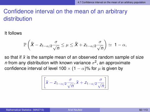
It follows
P(
X̄ − z1−α/2σ√n≤ µ ≤ X̄ + z1−α/2
σ√n
)' 1− α,
so that if x̄ is the sample mean of an observed random sample of sizen from any distribution with known variance σ2, an approximateconfidence interval of level 100× (1− α)% for µ is given by[
x̄ − z1−α/2σ√n, x̄ + z1−α/2
σ√n
]
Mathematical Statistics (MAS713) Ariel Neufeld 92 / 113

4.7 Confidence interval on the mean of an arbitrary population
Confidence interval on the mean of an arbitrarydistribution
Note : because this result requires “n large enough” to be reliable, thistype of interval, based on the CLT, is often called large-sampleconfidence interval
One could also define large-sample one-sided confidence intervals oflevel 100× (1− α)% : (−∞, x̄ + z1−α
σ√n ] and [x̄ − z1−α
σ√n ,+∞)
Mathematical Statistics (MAS713) Ariel Neufeld 93 / 113

4.7 Confidence interval on the mean of an arbitrary population
Confidence interval on the mean of an arbitrarydistribution
What if the population standard deviation is unknown ?
Mathematical Statistics (MAS713) Ariel Neufeld 94 / 113

4.7 Confidence interval on the mean of an arbitrary population
Confidence interval on the mean of an arbitrarydistribution
; as previously, it is natural to replace σ by the sample standarddeviation S and to work with
T =√
nX̄ − µ
S
One might then expect to base the derivation of the CI on T ∼ tn−1
Mathematical Statistics (MAS713) Ariel Neufeld 95 / 113
4.7 Confidence interval on the mean of an arbitrary population
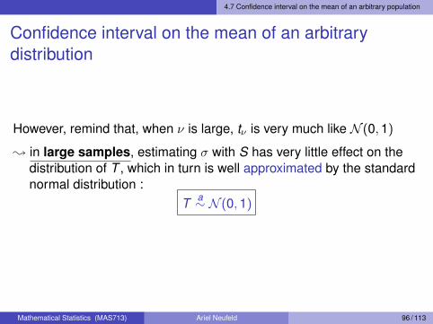
Confidence interval on the mean of an arbitrarydistribution
However, remind that, when ν is large, tν is very much like N (0,1)
; in large samples, estimating σ with S has very little effect on thedistribution of T , which in turn is well approximated by the standardnormal distribution :
T a∼ N (0,1)
Mathematical Statistics (MAS713) Ariel Neufeld 96 / 113

4.7 Confidence interval on the mean of an arbitrary population
Confidence interval on the mean of an arbitrarydistribution
Consequently, if x̄ and s are the sample mean and the samplestandard deviation of an observed random sample of size n from anydistribution, an approximate confidence interval of level100× (1− α)% for µ is given by[
x̄ − z1−α/2s√n, x̄ + z1−α/2
s√n
]This expression holds regardless of the population distribution, as longas n is large enough
As usual, corresponding one-sided confidence intervals could bedefined : (−∞, x̄ + z1−α
s√n ] and [x̄ − z1−α
s√n ,+∞)
Mathematical Statistics (MAS713) Ariel Neufeld 97 / 113

4.7 Confidence interval on the mean of an arbitrary population
Confidence interval on the mean of an arbitrarydistribution : exampleExampleA lab reports the results of a study to investigate mercury contaminationlevels in fish. A sample of 53 fish was selected from some Florida lakes, andmercury concentration in the muscle tissue was measured (in ppm) :
1.23, 0.49, 1.08, . . ., 0.16, 0.27Find a confidence interval of level 95% on µ, the mean mercury concentrationin the muscle tissue of fish
An histogram and a quantile plot for the datahistogram
concentration
Den
sity
0.0 0.2 0.4 0.6 0.8 1.0 1.2 1.4
0.0
0.2
0.4
0.6
0.8
1.0 ●
●●
●
●
●
●
●
●
●
●
●
●
●●
●
●
●
●
●
●
●
●
●
●
●
●
●
●
●
●
●
●
●
●
●
●
●
●
●
●
●
●
●
●●
●
●●
●
●●
●
0.0 0.2 0.4 0.6 0.8 1.0 1.2
−2
−1
01
2
Normal Q−Q Plot
Sample Quantiles
The
oret
ical
Qua
ntile
s
Mathematical Statistics (MAS713) Ariel Neufeld 98 / 113

4.7 Confidence interval on the mean of an arbitrary population
Confidence interval on the mean of an arbitrarydistribution : example; both plots indicate that the distribution of mercury concentration isnot normal (positively skewed)
However, the sample is large enough (n = 53) to use the CentralLimit Theorem and derive approximate confidence interval for µ
Elementary computations give x̄ = 0.525 ppm and s = 0.3486 ppm.A large sample confidence interval is given by[x̄ − z1−α/2
s√n , x̄ + z1−α/2
s√n
]With z0.975 = 1.96 and the above values, we have[
0.525− 1.960.3486√
53,0.525 + 1.96
0.3486√53
]= [0.4311,0.6189]
; we are ± 95% confident that the true average mercuryconcentration is between 0.4311 and 0.6189 ppm
Mathematical Statistics (MAS713) Ariel Neufeld 99 / 113
4.7 Confidence interval on the mean of an arbitrary population
Confidence intervals for the mean :summary
Mathematical Statistics (MAS713) Ariel Neufeld 100 / 113
4.7 Confidence interval on the mean of an arbitrary population
Confidence intervals for the mean : summary
The several situations leading to different confidence intervals for themean can be summarised as follows :
Mathematical Statistics (MAS713) Ariel Neufeld 101 / 113
4.7 Confidence interval on the mean of an arbitrary population
Confidence intervals for the mean : summary
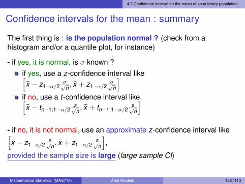
The first thing is : is the population normal ? (check from ahistogram and/or a quantile plot, for instance)
- if yes, it is normal, is σ known ?if yes, use a z-confidence interval like[x̄ − z1−α/2
σ√n , x̄ + z1−α/2
σ√n
]if no, use a t-confidence interval like[x̄ − tn−1;1−α/2
s√n , x̄ + tn−1;1−α/2
s√n
]- if no, it is not normal, use an approximate z-confidence interval like[x̄ − z1−α/2
s√n , x̄ + z1−α/2
s√n
],
provided the sample size is large (large sample CI)
Mathematical Statistics (MAS713) Ariel Neufeld 102 / 113

4.7 Confidence interval on the mean of an arbitrary population
Confidence intervals for the mean : summary
What if the sample size is small and the population is not normal ?; check on a case by case basis (beyond the scope of this course)
Mathematical Statistics (MAS713) Ariel Neufeld 103 / 113
4.8 Prediction intervals
Prediction intervals
Mathematical Statistics (MAS713) Ariel Neufeld 104 / 113

4.8 Prediction intervals
Prediction interval for a future observation
In some situations, we may be interested in predicting a futureobservation of a variable
; different than estimating the mean of the variable !
; instead of confidence intervals, we are after100× (1− α)% prediction interval on a future observation
Mathematical Statistics (MAS713) Ariel Neufeld 105 / 113

4.8 Prediction intervals
Prediction interval for a future observation
Suppose that X1,X2, . . . ,Xn is a random sample from a normalpopulation with mean µ and standard deviation σ
; we wish to predict the value Xn+1, a single future observation
As Xn+1 comes from the same population as X1,X2, . . . ,Xn,information contained in the sample should be used to predict Xn+1
; the predictor of Xn+1, say X ∗, should be a statistic
Mathematical Statistics (MAS713) Ariel Neufeld 106 / 113

4.8 Prediction intervals
Prediction interval for a future observation
Let’s define an estimator for µ as the sample mean, so we take it aspredictor :
X ∗ = X̄ =1n
n∑i=1
Xi
Now, let’s look at the error term
e = Xn+1 − X̄
X̄ ∼ N (µ,σ√n
)
Xn+1 ∼ N (µ, σ)
Mathematical Statistics (MAS713) Ariel Neufeld 107 / 113

4.8 Prediction intervals
Prediction interval for a future observation
So we have that
e ∼ N (µe, σe)
We have that µe = 0 andthe variance of the prediction error is
Var(e) = Var(Xn+1 − X ∗) = Var(Xn+1 − X̄ ) = Var(Xn+1) + Var(X̄ )
= σ2 + σ2
n = σ2 (1 + 1n
)(because Xn+1 is independent of X1,X2, . . . ,Xn and so of X̄ )
e ∼ N(
0,√σ2(1 + 1
n
))
Mathematical Statistics (MAS713) Ariel Neufeld 108 / 113

4.8 Prediction intervals
Prediction interval for a future observation
Hence,Z =
Xn+1 − X̄
σ√
1 + 1n
∼ N (0,1)
Replacing the possibly unknown σ with the sample standard deviationS yields
T =Xn+1 − X̄
S√
1 + 1n
∼ tn−1
Mathematical Statistics (MAS713) Ariel Neufeld 109 / 113

4.8 Prediction intervals
Prediction interval for a future observation
Manipulating Z and T as we did previously for CI leads to the100× (1− α)% z- and t-prediction intervals on the future observation :[
x̄ − z1−α/2 σ√
1 + 1n , x̄ + z1−α/2 σ
√1 + 1
n
][x̄ − tn−1;1−α/2 s
√1 + 1
n , x̄ + tn−1;1−α/2 s√
1 + 1n
]
Mathematical Statistics (MAS713) Ariel Neufeld 110 / 113

4.8 Prediction intervals
Prediction interval for a future observation : remarks
Remark 1 :
Prediction intervals for a single observation will always be longer thanconfidence intervals for µ, because there is more variability associatedwith one observation than with an average
Mathematical Statistics (MAS713) Ariel Neufeld 111 / 113
4.8 Prediction intervals
Prediction interval for a future observation : remarks
Remark 2 :
As n gets larger (n→∞):
the width of the CI for µ decreases to 0(we are more and more accurate when estimating µ),
but
this is not the case for a prediction interval :the inherent variability of Xn+1 never vanishes, even when we haveobserved many other observations before!
Mathematical Statistics (MAS713) Ariel Neufeld 112 / 113

ObjectivesNow you should be able to :
Understand the basics of interval estimation
Explain what a confidence interval of level 100 × (1 − α)% for a given parameteris
Construct confidence intervals on the mean of a normal distribution, advisedlyusing either the normal distribution or the Student’s t distribution
Understand the Central Limit Theorem
Explain the important role of the normal distribution as a sampling distribution
Construct large sample confidence intervals on a mean of an arbitrarydistribution
Explain the difference between a confidence interval and a prediction interval
Construct prediction intervals for a future observation in a normal population
Put yourself to the test ! ; Q34 p.457, Q35 p.457, Q57 p.462, Q57 p.462,
Mathematical Statistics (MAS713) Ariel Neufeld 113 / 113