Mathematical Statistics II: Demystifying statisticssuhasini/teaching415/chapter1.pdf ·...

TAMU, STAT 415

Mathematical Statistics II: Demystifying statistics

Suhasini Subba Rao

Spring, 2020

Contents

Contents

1 Introduction and Review 41.1 Why we spoil statistics with maths . . . . . . . . . . . . . . . . . . . . . . . . . . . . . . . 41.2 Joint distributions of random variables . . . . . . . . . . . . . . . . . . . . . . . . . . . . . 71.3 Euclidean space and matrix multiplication . . . . . . . . . . . . . . . . . . . . . . . . . . . 9

1.3.1 Inner (scalar) products and projections . . . . . . . . . . . . . . . . . . . . . . . . . 91.3.2 Orthonormal basis expansion . . . . . . . . . . . . . . . . . . . . . . . . . . . . . . 111.3.3 Matrix multiplication . . . . . . . . . . . . . . . . . . . . . . . . . . . . . . . . . . . 14

1.4 Expectation, variance and covariance . . . . . . . . . . . . . . . . . . . . . . . . . . . . . . 161.4.1 Expectation . . . . . . . . . . . . . . . . . . . . . . . . . . . . . . . . . . . . . . . . 161.4.2 Example: Interpreting the covariance of bivariate data . . . . . . . . . . . . . . . . 171.4.3 The variance matrix . . . . . . . . . . . . . . . . . . . . . . . . . . . . . . . . . . . 191.4.4 Properties of the variance . . . . . . . . . . . . . . . . . . . . . . . . . . . . . . . . 21

1.5 Modes of convergence . . . . . . . . . . . . . . . . . . . . . . . . . . . . . . . . . . . . . . . 231.5.1 The mean squared error . . . . . . . . . . . . . . . . . . . . . . . . . . . . . . . . . 241.5.2 Convergence in probability . . . . . . . . . . . . . . . . . . . . . . . . . . . . . . . 271.5.3 Sampling distributions and the central limit theorem . . . . . . . . . . . . . . . . . 271.5.4 Functions of sample means . . . . . . . . . . . . . . . . . . . . . . . . . . . . . . . 33

1.6 A historical perspective . . . . . . . . . . . . . . . . . . . . . . . . . . . . . . . . . . . . . . 36

2 Classical distributions and the first foray into sampling distributions 372.1 The Multivariate Gaussian distribution . . . . . . . . . . . . . . . . . . . . . . . . . . . . . 372.2 Relatives of the Gaussian distribution . . . . . . . . . . . . . . . . . . . . . . . . . . . . . . 40

2.2.1 The chi-square distribution . . . . . . . . . . . . . . . . . . . . . . . . . . . . . . . 402.2.2 The t-distribution . . . . . . . . . . . . . . . . . . . . . . . . . . . . . . . . . . . . . 412.2.3 The F-distribution . . . . . . . . . . . . . . . . . . . . . . . . . . . . . . . . . . . . 43

2.3 The exponential class of distributions . . . . . . . . . . . . . . . . . . . . . . . . . . . . . . 432.4 The sample mean and variance: Sampling distributions . . . . . . . . . . . . . . . . . . . . 47

2.4.1 The sample mean . . . . . . . . . . . . . . . . . . . . . . . . . . . . . . . . . . . . . 472.4.2 The sample variance . . . . . . . . . . . . . . . . . . . . . . . . . . . . . . . . . . . 472.4.3 The t-statistic . . . . . . . . . . . . . . . . . . . . . . . . . . . . . . . . . . . . . . . 58

2

Contents2.4.4 A historical perspective . . . . . . . . . . . . . . . . . . . . . . . . . . . . . . . . . 62

3 Parameter Estimation 633.1 Introduction . . . . . . . . . . . . . . . . . . . . . . . . . . . . . . . . . . . . . . . . . . . . 633.2 Estimation: Method of moments . . . . . . . . . . . . . . . . . . . . . . . . . . . . . . . . . 64

3.2.1 Motivation . . . . . . . . . . . . . . . . . . . . . . . . . . . . . . . . . . . . . . . . . 643.2.2 Examples . . . . . . . . . . . . . . . . . . . . . . . . . . . . . . . . . . . . . . . . . 663.2.3 Sampling properties of method of moments estimators . . . . . . . . . . . . . . . . 67

3.3 Monte Carlo methods . . . . . . . . . . . . . . . . . . . . . . . . . . . . . . . . . . . . . . . 703.3.1 The parametric Bootstrap . . . . . . . . . . . . . . . . . . . . . . . . . . . . . . . . 713.3.2 The nonparametric Bootstrap . . . . . . . . . . . . . . . . . . . . . . . . . . . . . . 723.3.3 The power transform approach . . . . . . . . . . . . . . . . . . . . . . . . . . . . . 74

3.4 Estimation: Maximum likelihood (MLE) . . . . . . . . . . . . . . . . . . . . . . . . . . . . . 753.4.1 Motivation . . . . . . . . . . . . . . . . . . . . . . . . . . . . . . . . . . . . . . . . . 753.4.2 Examples . . . . . . . . . . . . . . . . . . . . . . . . . . . . . . . . . . . . . . . . . 773.4.3 Evaluation of the MLE for more complicated distributions . . . . . . . . . . . . . . 84

3.5 Sampling properties of the MLE . . . . . . . . . . . . . . . . . . . . . . . . . . . . . . . . . 863.5.1 Consistency . . . . . . . . . . . . . . . . . . . . . . . . . . . . . . . . . . . . . . . . 863.5.2 The distributional properties of the MLE . . . . . . . . . . . . . . . . . . . . . . . . 873.5.3 The Fisher information matrix . . . . . . . . . . . . . . . . . . . . . . . . . . . . . . 933.5.4 The curious case of the uniform distribution . . . . . . . . . . . . . . . . . . . . . . 96

3.6 What is the best estimator? . . . . . . . . . . . . . . . . . . . . . . . . . . . . . . . . . . . . 973.6.1 Measuring e�ciency . . . . . . . . . . . . . . . . . . . . . . . . . . . . . . . . . . . 973.6.2 The Cramer-Rao Bound . . . . . . . . . . . . . . . . . . . . . . . . . . . . . . . . . 99

3.7 Su�ciency . . . . . . . . . . . . . . . . . . . . . . . . . . . . . . . . . . . . . . . . . . . . . 1003.7.1 Application of su�ciency to estimation: Rao-Blackwellisation . . . . . . . . . . . . 104

3.8 What happens if we get the assumptions wrong . . . . . . . . . . . . . . . . . . . . . . . . 1053.9 A historical perspective . . . . . . . . . . . . . . . . . . . . . . . . . . . . . . . . . . . . . . 105

4 Comparing two populations 1064.1 The independent two sample test . . . . . . . . . . . . . . . . . . . . . . . . . . . . . . . . 1064.2 Constructing the Likelihoods under the null and alternative . . . . . . . . . . . . . . . . . 106

4.2.1 Transformation of the data . . . . . . . . . . . . . . . . . . . . . . . . . . . . . . . 1064.2.2 Relationship to the log-likelihood ratio test . . . . . . . . . . . . . . . . . . . . . . 109

5 ANOVA 1125.1 Proof of one-way ANOVA . . . . . . . . . . . . . . . . . . . . . . . . . . . . . . . . . . . . 112

3

1 Introduction and Review


1.1 Why we spoil statistics with maths

To understand the aims and objectives of this course, we start with a motivating example. Weather stationsaround the world are constantly collecting data (temperature, air pressure and ozone levels to name but afew). To publish this data in a coherent fashion, it is often summarized, in such a way that one easily �ndspertinent trends. For example, if you search for temperature data on the web, you will usually �nd that themonthly average temperature (at a particular longitude and latitude) is published.

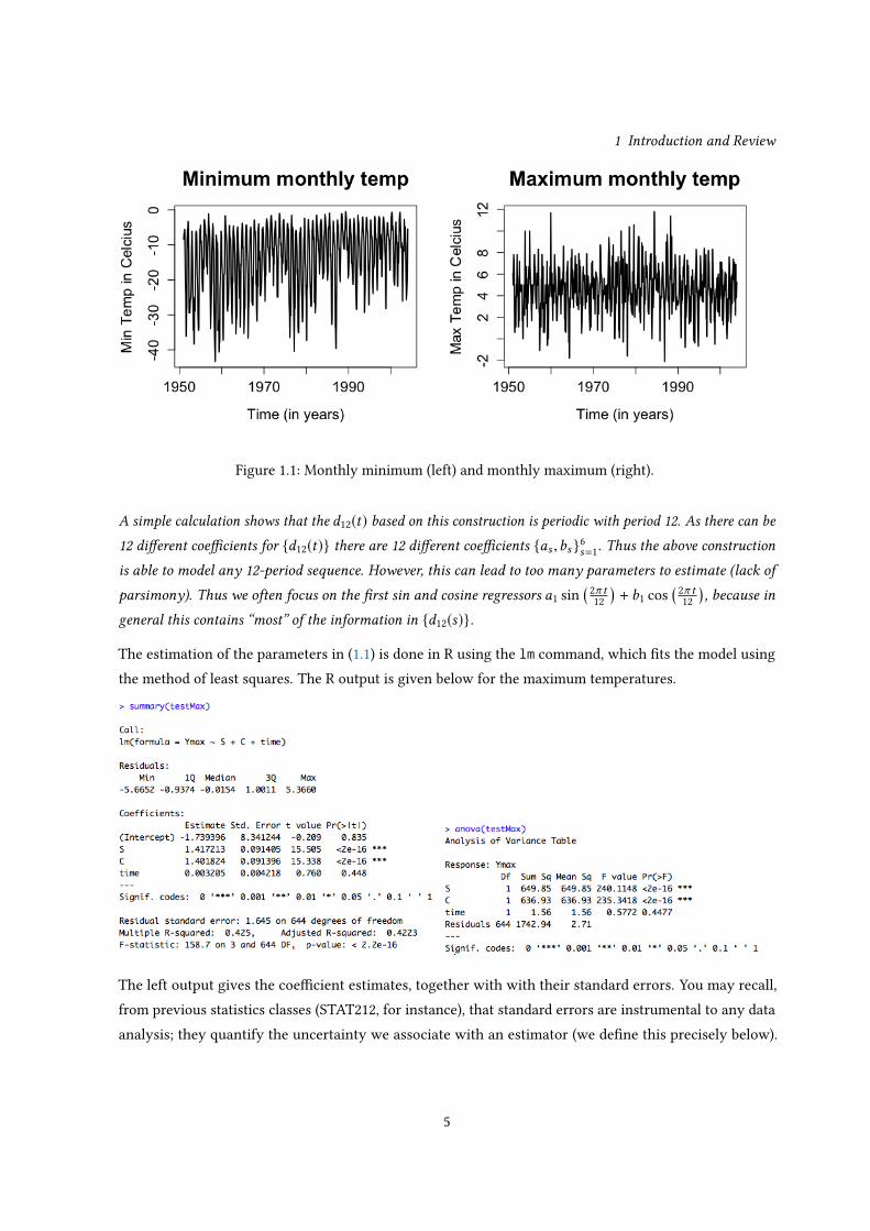
Over the past thirty years or so, scientists have been monitoring the temperatures in Antarctica. Theconcern is that rises in temperatures in this region will lead to a melting of glaciers and rises in oceanlevels. Therefore, we focus our attention on the temperatures collected at Faraday station (later called theVernadsky research base: a brief history can be found here https://www.bas.ac.uk/about/about-bas/history/british-research-stations-and-refuges/faraday-f/), which has a long history of climaticresearch (dating back to 1947). From 1951-2004, the monthly temperatures have been published by theBritish Antarctic Survey. What makes their data set quite unique is that they collect the monthly extremes(max and mins) not just the averages. A plot of the monthly extremes is given in Figure 1.1. As our aim isto understand if the temperatures are rising, we regress the minimum and maximum temperatures againsttime. However, as this is monthly data, it will have a clear seasonality and that too must be included inthe regression. This often done by including a seasonal component in the regression model such as a sineand cosine function with a 12 month period. Thus we �t the following linear regression model to both themaximum and minimum temperatures

�t = �0 + �S sin✓2�t12

◆+ �C cos

✓2�t12

◆+ �2t + �t (1.1)

to the data.

Remark (Modelling periodicities). Monthly temperatures are likely to be periodic with a period of 12months. A

periodic sequence, with a period of 12 months is a sequence {d12(t)} whered12(t) = d12(t+12) = d12(t+24) = . . .for all t . We can model all period sequences with a period of 12 months using sin and cosine functions;

d12(t) =6’

s=1

✓as sin

✓2�t12

s

◆+ bs cos

✓2�t12

s

◆◆.

4


Figure 1.1: Monthly minimum (left) and monthly maximum (right).

A simple calculation shows that the d12(t) based on this construction is periodic with period 12. As there can be

12 di�erent coe�cients for {d12(t)} there are 12 di�erent coe�cients {as ,bs }6s=1. Thus the above constructionis able to model any 12-period sequence. However, this can lead to too many parameters to estimate (lack of

parsimony). Thus we often focus on the �rst sin and cosine regressors a1 sin� 2� t12

�+ b1 cos

� 2� t12

�, because in

general this contains “most” of the information in {d12(s)}.

The estimation of the parameters in (1.1) is done in R using the lm command, which �ts the model usingthe method of least squares. The R output is given below for the maximum temperatures.

The left output gives the coe�cient estimates, together with with their standard errors. You may recall,from previous statistics classes (STAT212, for instance), that standard errors are instrumental to any dataanalysis; they quantify the uncertainty we associate with an estimator (we de�ne this precisely below).

5

1 Introduction and ReviewAnd to determine if a coe�cient is statistically signi�cant we calculate the ratio

t value =EstimateStd. Error

,

where signi�cance of each individual coe�cient can be determined by using a t-test (this is the p-valuegiven in Pr(> |t |)). The analysis of the variance on the right measures the reduction in the squared error aseach variable is added to the model. The bigger and more dramatic the reduction the smaller the p-value asgiven by Pr(> F ). Studying the p-values we observe that the seasonal terms (sin and cosine) are statisticallysigni�cant. However, despite the time coe�cient being positive, there is no signi�cant evidence of anincrease in the temperatures over time (observe the large p-value corresponding to time in both outputs.Recall when there is no statistical evidence of an increase there are two possible explanations (a) therereally is no increase or (b) the noise in the data is too large, that it is masks an increase.

We conduct a similar analysis using the minimum temperatures. The output is given below

Studying the p-values in this output we observe that the seasonal component is statistically signi�cantand also the linear increase in temperatures over time. The data suggests that there is an increase in themonthly minimum temperatures over time. This is very interesting. To summarize, there is no evidence ofan increase in the monthly maximum temperatures, but there is evidence of an increase in the minimumtemperatures. But before we make any such conclusions, we have to decide if the analysis is valid. Thismeans taking a step back and understanding where all the standard errors, p-values etc come from. If theyhave been calculated incorrectly, then the conclusions of the analysis may be wrong.

First we make a plot of a histogram of the residuals

b�t = �t � b�0 � b

�S,1 sin✓2�t12

◆� b�C,1 cos

✓2�t12

◆� b�2t .

This is given in Figure 1.2. We observe that the distribution of the residuals of the maximum temperatureslook symmetric, but the distribution of the residuals of the minimum temperatures appear left skewed.

6


Figure 1.2: Histogram of residuals: Minimum of left and maximum of right.

(1) Clearly the residuals for the minimum temperatures are not normal (the normal/Gaussian distributionis symmetric). Does that matter, do we require normality for the analysis?

(2) What about the standard errors, how are they calculated? How, was the data collected? The datahas been collected over time. Often data that has been collected over time, are dependent. Theindependence assumption probably does not hold. To demonstrate that there is possible dependence,the estimated autocorrelation (ACF) plot of the residuals is given in Figure 1.3. We observe whatappears to be dependence (this is beyond this course, and will be discussed in a time series course).Does dependence in�uence the standard errors? If it does, where will it e�ect the conclusions of thestudy?

Though we cannot answer, all the above questions in this course; time series data tends to be extremelycomplex. In this course, we will hopefully understand why things work. And if we understand why theywork, we can also understand when procedures may not work, and how it can in�uence the conclusionsthat we draw.

1.2 Joint distributions of random variables

Please Review STAT 414, and pay particular attention to the joint distribution of discrete and continuousrandom variables. We give a quick summary of what you need to know. Suppose that X = (X1, . . . ,Xn) is adiscrete random vector. Then their joint probability mass function is

pX (x1,x2, . . . ,xn) = PX (X1 = x1, . . . ,Xn = xn).

7


Figure 1.3: The estimated autocorrelation plot of the minimum residuals.

Suppose that (X1, . . . ,Xn) is a vector of continuous random variables then the joint density is a piecewisecontinuous function fX (x1, . . . ,xn) where

PX ((X1,X2, . . . ,Xn) 2 A) =πAfX (x1, . . . ,xn)dx1 . . .dxn .

De�nition 1.1 (Independence). The random variables X1,X2, . . . ,Xn are said to be independent if their joint

distribution (or density) function can be written as the product of their marginal distributions

FX1, ...,Xn (x1, . . . ,xn) = FX1(x1)FX2(x2) . . . FXn (xn) for all x1, . . . ,xn .

Below, we generalize the above notion to independence between vectors.De�nition 1.2. Suppose Y = (Y1, . . . ,Yp ) and X = (X1, . . . ,Xq) are random vectors. X and Y are said to be

independent if joint cumalative distribution function of X and Y can be written as the product of the joint

distributions

FX ,Y (x ,�) = FX (x)FY (�).

De�nition 1.3 (iid). The random variables {Xi }ni=1 are said to be independent and identically distributed (iid

for short) if {Xi }ni=1 are independent and the marginal distribution is the same for all the random variables.

Remark (Conditional probabilities). We recall that the conditional probability of event A given B is

P(A|B) = P(A \ B)P(B) .

The two events A and B are statistically independent if P(A|B) = P(A) (occurence of event B has no impact on

the probability of event A). Suppose A is an event corresponding to random variables X (technically we say

8

1 Introduction and Reviewthat A belongs to a sigma-algebra generated by X , but this is not a technical course) and B corresponds to the

random variable Y . If X and Y are independent random variables as de�ned above, then P(A|B) = P(A) and Aand B are independent events.

1.3 Euclidean space and matrix multiplication

In this section we review some results from linear algebra, focusing on this simple case of �nite dimensionEuclidean space. In statistics we store data as vectors (or matrices), therefore either implicitly or explictly weare manipulating vectors. A solid understanding of linear algebra will help in both the mathematical proofsbut also writing good and fast pieces of code. For example, the empirical correlation can be understoodin terms of projections of one vector onto another. Thus rather than a code the correlation as an n-loop(which takes time) we can simply write it as dot/scalar/inner product which is computationally faster.

Reminder: if � is a scalar (a number) and x is a vector, then

�

©≠≠≠≠≠≠´

x1

x2...

xd

™ÆÆÆÆÆÆ¨=

©≠≠≠≠≠≠´

�x1

�x2...

�xd

™ÆÆÆÆÆÆ¨.

1.3.1 Inner (scalar) products and projections

We de�ne the inner product (also called the scalar product) between the vector x 2 Rd and � 2 Rd as

hx ,�i =d’i=1

xi�i .

Observe that by de�nition hx ,�i = h� ,x i (the inner product is symmetric). Inner products satisfy somebasic properties. The one we will use is

h�x + �z,�i = � hx ,�i + � hz,�i

where � , � 2 R, which is easily veri�ed. The Euclidean distance is the length of the vector x , and is

kx k =phx ,xi =

qÕdi=1 x

2i (this is easily understood by considering vectors on R2 and measuring the

distance from the origin (0, 0) to the vector). Often it is useful to deal with the the standardized vector

x

kx k .

The standardisation means that the length of this vector (its Euclidean distance) is one. In Euclidean space,inner products have a useful geometric properties. We state these below.

9

1 Introduction and ReviewRemark (Interpreting a zero inner product). If hx ,�i = 0, then x and � are orthogonal. This means the angle

between the two vectors is 90 degrees. In R2 there will only be one vector (up to a scalar constant) � that is

orthogonal to x . In R3 a plane is orthogonal to x .

De�nition 1.4 (Projection). The projection of � onto x is �x , where the value � such that the innerproduct

between � � �x and x is zero. The value � is obtained by solving

h � � �x| {z }red dashed line

,xi = 0

= h�,xi � � hx ,xi = 0 ) � =h�,xihx ,xi =

h�,xikx k2 .

We give an example for dimension d = 2. Consider the vectors x and � where

� =

21

!and x =

1/41/2

!.

The vectors � and x are the blue line and dashedblue line on the plot. The standardized vector x

kx k =

5�1/2(1, 2)0 is the yellow point on the plot. The projec-tion of � onto the line {�x ;� 2 (�1,1)} is the redpoint on the yellow dashed line which is orthogonalwith the red dashed line in the plot. This point is �xwhere

� =h�,xikx k2 =

165= 3.2.

Observe that h�,xi can be viewed as a measure of similarity between the vectors x and �. If h�,xi = 0, thevectors are orthogonal and there is no similarity between the vectors.

In the next section we describe the orthogonal representation of vectors. We have already come across this,in the above example. The yellow projection vector (4/5, 8/5)0 and the red vector (6/5,�3/5) are orthogonal(observe that they are at right angles). They form the building blocks of �:

� =

21

!=

4/58/5

!

| {z }=�x

+

6/5�3/5

!.

10

1 Introduction and Review1.3.2 Orthonormal basis expansion

The vectors e1 = (1, 0, 0), e2 = (0, 1, 0) and e3 = (0, 0, 1) form what is called an orthonormal basis (de�nedbelow) ofR3. It is clear that any� = (�1,�2,�3) 2 R3 can writen as� = �1e1+�2e2+�3e3 (a linear combinationof the basis). However, this basis is far from unique. We can rewrite � in terms of any orthonormal basis.Below we show how this possible using the idea of projections de�ned in the previous section.

The d-vectors {e j }dj=1 is an orthonormal basis of Rd if for all 1 i, j d we have

hei , e j i =(

1 i = j

0 i , j

.

Note from above, the length of the vectors are hei , ei i = kei k2 = 1. Orthonormal basis are not unique (thereare an uncountable number of di�erent orthonormal basis on Rd ).

For a given orthonormal basis {e j }dj=1 in Rd , we now show that we can decompose any vector � 2 Rd as aweighted sum of the orthogonal basis. This is easily seen by using the projection argument given in theprevious section. Projecting � onto e1 gives

�1 =h�, e1ike1k2

= h�, e1i.

The remainder (residual) is � � h�, e1ie1 (which is orthogonal to e1). Next we project � � �1e1 onto e2. Thisgives the coe�cient

�2 =h� � �1e1, e2i

ke2k2=

h�, e2i � �1he1, e2ike2k2

= h�, e2i.

Thus the residual after projecting on e1 and e2 is

� � �1e1 � �2e2.

Iterating this we obtain the orthonormal basis expansion

� =

d’j=1

h� , e j ie j .

Thus we have decomposed� into vectors into orthogonal building block. Each coe�cient � j h� , e j i describesthe how much of the vector e j is required to build �. Rewriting � in terms of a basis {e j }dj=1 is the same wewriting � in terms of a rotation of the usually axis.

Remark (Projection onto planes in Rd ). Suppose that {e j }dj=1 is an orthonormal basis of Rd , and de�ne the

plane, �, as all linear combination of the vectors {e j }rj=1 (where r < d) i.e.

� =

(r’s=1

�se j ; �1, . . . ,�r 2 R).

11

1 Introduction and ReviewSince {e j }sj=1 are orthogonal, the projection of � 2 Rd onto � can be done sequentially by projecting onto each

es , this gives the projection

P�(�) =r’s=1

hes ,�ies .

Example 1.1 (Examples of orthonormal basis on R

2). (i) The simplest example is

e1 =

10

!, e2 =

01

!

Clearly for any x2 2 R2 we have

x2 = x1e1 + x2e2.

(ii) Another orthonormal basis is

e1 =1p2

11

!, e2 =

1p2

1�1

!,

It is easy to show that he1, e2i = (1 � 1)/2 = 0. For the purpose of visualisation, it is useful to plot thebasis.

Using the above basis, any vector x 0 = (x1,x2) 2 R2 can be written as

x =

x1

x2

!= hx , e1ie1 + hx , e2ie2

=

✓ (x1 + x2)p2

◆1p2

11

!+

✓ (x1 � x2)p2

◆1p2

1�1

!.

Example 1.2 (Examples of orthonormal basis on R

3). (i) The simplest example is

e1 =©≠≠≠´

100

™ÆÆÆ¨, e2 =

©≠≠≠´

010

™ÆÆÆ¨, e3 =

©≠≠≠´

001

™ÆÆÆ¨

(ii) An alternative orthonormal basis is

e1 =1p3

©≠≠≠´

111

™ÆÆÆ¨, e2 =

1p2

©≠≠≠´

01�1

™ÆÆÆ¨, e3 =

1p6

©≠≠≠´

�211

™ÆÆÆ¨

Again you can show that he1, e2i = he1, e3i = he2, e3i = 0 (please do this).

12

1 Introduction and ReviewUsing the above basis, any vector x 2 R3 can be written as

©≠≠≠´

x1

x2

x2

™ÆÆÆ¨= hx , e1ie1 + hx , e2ie2 + hx , e3ie3

=

✓x1 + x2 + x3p

3

◆1p3

©≠≠≠´

111

™ÆÆÆ¨+

✓x2 + x3p

2

◆1p2

©≠≠≠´

01�1

™ÆÆÆ¨+

✓�2x1 + x2 + x3p6

◆1p6

©≠≠≠´

�211

™ÆÆÆ¨.

One way to construct the above basis is to use properties of sins and cosines;

e2 =1p2

©≠≠≠´

cos(2� ⇥ 0/3)cos(2� ⇥ 1/3)cos(2� ⇥ 2/3)

™ÆÆÆ¨⇡ 1

1.5

©≠≠≠´

1�0.5�0.5

™ÆÆÆ¨and e3 =

1p2

©≠≠≠´

sin(2� ⇥ 0/3)sin(2� ⇥ 1/3)sin(2� ⇥ 2/3)

™ÆÆÆ¨⇡ 1p

1.5

©≠≠≠´

00.866�0.866

™ÆÆÆ¨.

Parseval’s identity

We will use the representation

� =

d’j=1

h�, e j ie j ,

to write the Euclidean distance interms of � in terms of h�, e j i. First observe that if the basis is e1 =(1, 0, 0, . . . , 0), e2 = (0, 1, 0, . . . , 0),. . ., ed = (0, 0, 0, . . . , 1), then it is clear that

Õdj=1�

2j =

Õnj=1h�, e j i2 (since

h�, e j i2 = �2j ). We show below that this is true for any orthonormal basis:

d’j=1

�

2j = h�,�i

=

d’j1, j2=1

h�, e j1ih�, e j1ihe j1 , e j2i

=

d’j=1

h�, e j i2. (1.2)

This is called Parseval’s identity.

A useful extension to the above inequality is the following result

k� � h�, e1ie1k =d’j=2

h�, e j i2.

The proof follows the same argument as that given above.

13

1 Introduction and ReviewWe now give a useful application of this result. Suppose e1 = d

�1/2(1, . . . , 1), then h�, e1i = d�1/2Õd

j=1�j =

d

1/2� (where � is the average of the elements in �). Thus

h�, e1ie1 = d1/2�d�1/2(1, . . . , 1) = �(1, . . . , 1).

Therefore

� � h�, e1ie1 = (�1 � �,�2 � �, . . . ,�d � �).

Suppose {e j }dj=2 are orthonormal to e1, then we have

k� � h�, e1ie1k =d’j=1

(�j � �)2 =d’j=2

h�, e j i2. (1.3)

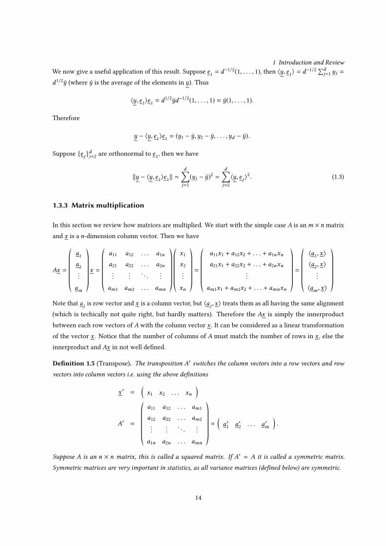
1.3.3 Matrix multiplication

In this section we review how matrices are multiplied. We start with the simple case A is anm ⇥ n matrixand x is a n-dimension column vector. Then we have

Ax =

©≠≠≠≠≠≠´

a1

a2...

am

™ÆÆÆÆÆÆ¨x =

©≠≠≠≠≠≠´

a11 a12 . . . a1n

a21 a22 . . . a2n...

.... . .

...

am1 am2 . . . amn

™ÆÆÆÆÆÆ¨

©≠≠≠≠≠≠´

x1

x2...

xn

™ÆÆÆÆÆÆ¨=

©≠≠≠≠≠≠´

a11x1 + a12x2 + . . . + a1nxn

a21x1 + a22x2 + . . . + a2nxn...

am1x1 + am2x2 + . . . + amnxn

™ÆÆÆÆÆÆ¨=

©≠≠≠≠≠≠´

ha1,xiha2,xi...

ham ,xi

™ÆÆÆÆÆÆ¨

Note that aj is row vector and x is a column vector, but haj ,xi treats them as all having the same alignment(which is techically not quite right, but hardly matters). Therefore the Ax is simply the innerproductbetween each row vectors of A with the column vector x . It can be considered as a linear transformationof the vector x . Notice that the number of columns of A must match the number of rows in x , else theinnerproduct and Ax in not well de�ned.

De�nition 1.5 (Transpose). The transposition A

0 switches the column vectors into a row vectors and row

vectors into column vectors i.e. using the above de�nitions

x

0 =⇣x1 x2 . . . xn

⌘

A

0 =

©≠≠≠≠≠≠´

a11 a12 . . . am1

a12 a22 . . . am2...

.... . .

...

a1n a2n . . . amn

™ÆÆÆÆÆÆ¨=

⇣a

01 a

02 . . . a

0m

⌘.

Suppose A is an n ⇥ n matrix, this is called a squared matrix. If A0 = A it is called a symmetric matrix.

Symmetric matrices are very important in statistics, as all variance matrices (de�ned below) are symmetric.

14

1 Introduction and ReviewBased on the above de�nition we observe

(Ax)0 = x

0A

0 =⇣ha1,xi ha2,xi . . . ham ,xi

⌘.

Further if � is am-dimension column vector, then

�

0Ax =

m’i=1

�i hai ,xi =m’i=1

n’j=1

ai, j�ix j .

Example 1.3. Suppose x = (x1,x2, . . . ,xn)0.

(i) Then xx 0 is an n ⇥ n matrix:

xx

0 =

©≠≠≠≠≠≠´

x1

x2...

xn

™ÆÆÆÆÆÆ¨

⇣x1 x2 . . . xn

⌘=

©≠≠≠≠≠≠≠≠≠´

x

21 x1x2 . . . x1xn

x2x1 x

22 . . . x2xn

x3x1 x3x2 . . . x3xn...

.... . .

...

xnx1 xnx2 . . . x

2n

™ÆÆÆÆÆÆÆÆÆ¨

(ii) Then x 0x is a scalar:

x

0x =

⇣x1 x2 . . . xn

⌘ ©≠≠≠≠≠≠´

x1

x2...

xn

™ÆÆÆÆÆÆ¨= x

21 + x

22 + . . . + x

2n = hx ,xi.

We can generalize this notion to the product of them ⇥ n matrix A and n ⇥ p matrix B as follows

AB =

©≠≠≠≠≠≠´

a1

a2...

am

™ÆÆÆÆÆÆ¨

⇣b1,b2, . . . ,bp

⌘=

©≠≠≠≠≠≠´

a11 a12 . . . a1n

a21 a22 . . . a2n...

.... . .

...

am1 am2 . . . amn

™ÆÆÆÆÆÆ¨

©≠≠≠≠≠≠´

b11 b12 . . . b1p

b21 b22 . . . b2p...

.... . .

...

bn1 bn2 . . . bnp

™ÆÆÆÆÆÆ¨

=

©≠≠≠≠≠≠´

ha1,b1i ha1,b2i . . . ha1,bpiha2,b1i ha2,b2i . . . ha2,bpi...

.... . .

...

ham ,b1i ham ,b2i . . . ham ,bpi

™ÆÆÆÆÆÆ¨

ThusAB is comprised ofmp innerproducts. The number of columns inAmust match the number of columnsin B, else AB is not well de�ned.

Clearly AB is not commutative (in general, you cannot change the order: AB , BA)

Transpose: Observe the general identity:

(AB)0 = B

0A

0.

15

1 Introduction and Review1.4 Expectation, variance and covariance

1.4.1 Expectation

Statisticians almost always deal with averages of a sample. This is because the averages (in most situations)converge to its corresponding expectation. We start with the de�nition of the average and then de�ne theexpectation (we completely avoid the use of measures, sigma algebras etc).

Suppose the random variable X is a discrete valued random variable1 taking values {ki } and distributionp(ki ). Suppose we observe multiple realisations {xi }, then the averages

1n

n’i=1

xi and1n

n’i=1

�(xi )

will (almost surely) limit to the following “expectation”:

E[X ] =1’i=0

kip(ki ) and in general E[�(X )] =1’i=0

�(ki )p(ki ).

respectively, where � is any function. This is called the expectation of the random variable X and �(X ). If Xis a continuous value random2 variable with density f (x) then the expectation of X and �(X ) is

E[X ] =πRx f (x)dx and in general E[�(X )] =

π�(x)f (x)dx .

The expection can easily generalised to a vector by taking the expectation entrywise. Let X = (X1, . . . ,Xd )be a random row vector, then

E(X ) =⇣E(X1) E(X2) . . . E(Xd )

⌘=

⇣µ1 µ2 . . . µd

⌘= µ

The joint expectation, E(XY ), generalizes the above de�nition, and is taken over the joint distribution of(X ,Y ).Lemma 1.1 (Expectation of products of independent random variables). Suppose that X and Y are indepen-

dent random variables. Then

E(XY ) = E(X )E(Y ).

Example 1.4 (Expectations of mixtures). In statistics often modelling data with mixtures of distributions is

useful. Let X , Y and U be independent random variables. Let U be a Bernoulli random variable U 2 {0, 1},where P(U = 0) = p and P(U = 1) = 1 � p. De�ne the new random variable

Z = UX + (1 �U )Y .

1For example, the binomial or Poisson distribution.2For example, the normal distribution

16

1 Introduction and ReviewThe expectation

E[Z ] = E[UX + (1 �U )Y |U = 0]P(U = 0) + E[UX + (1 �U )Y |U = 1]P(U = 1)

= E[(1 �U )Y |U = 0]P(U = 0) + E[UX |U = 1]P(U = 1)

= pE[Y ] + (1 � p)E[X ].

By a similar argument we have Z 2 = (UX + (1 �U )Y )2 = (U 2X

2 + (1 �U )2Y 2 + 2U (1 �U )XY

E[Z 2] = E[(Z 2 |U = 0]P(U = 0) + E[Z 2 |U = 1]P(U = 1)

= E[(1 �U )2Y 2 |U = 0]P(U = 0) + E[U 2X

2 |U = 1]P(U = 1)

= pE[Y 2] + (1 � p)E[X 2].

1.4.2 Example: Interpreting the covariance of bivariate data

Suppose we observe the bivariate data �0.262.78

!,

�1.510.25

!,

�0.86�1.89

!, . . . ,

3.787.17

!,

In total we observe 200 vectors.

On the right we have made a scatter plot of the abovedata set. Clearly, there appears to be some sort of “lin-ear” dependence between the the two variables. Howto measure this? One solution is to use the similar-ity measure (inner product) described in the previoussection.

To do this, we rewrite the bivariate vectors as two 200-dimension vectors

x = (x1,x2, . . . ,x200) =⇣�0.26, �1.51, �0.86, . . . 3.78

⌘

� = (�1,�2, . . . ,�200) =⇣2.78, 0.25, �1.89, . . . 7.17

⌘,

If the vectors are “similar” they will almost lie on the same line and have a “large” inner product. We �rstcentralize the vectors by subtracting the average for each vector and then evaluate the (average) inner

17

1 Introduction and Reviewproduct

n

�1hx � x1,� � �1i = 1n

200’i=1

(xi � x)(�i � �)

which in this example is 4.7. If (Xi ,Yi ) are iid realisation from a distribution, the by the discussion in Section1.4.1, as we increase the number of realisation the above estimates the following expection

E [(X � E(X ))(Y � E(Y ))] .

This is called the covariance between the random variables X and Y . By a similar argument the averagesquared spread of the data is

1n

n’i=1

(xi � x)2 and 1n

n’i=1

(�i � �)2,

which for this example is 5.9 and 6.7 respectively. Taking the limit of the above over all possible realisationswe have

var(X ) = E (X � E(X ))2 and var(Y ) = E (Y � E(Y ))2 ,

which is called the variance of the random variables X and Y respectively.

We recall that in Section 1.3.1 we discuss standardized vectors. Where we divide a vector by the distance toensure it has a length one. We do this to our data vectors x and �:

(x1 � x ,x2 � x , . . . ,xn � x)pÕni=1(xi � x)2

(�1 � �,�2 � �, . . . ,�n � �)pÕni=1(�i � �)2

.

Then the projection of one vector onto the other (it does not matter which way round it is) isÕn

i=1(x1 � x)(�i � �)pÕni=1(xi � x)2 Õn

i=1(�i � �)2=

n

�1 Õni=1(x1 � x)(�i � �)p

n

�1 Õni=1(xi � x)2n�1 Õn

i=1(�i � �)2.

This measures the linear dependence between the two vectors, after taking into account their length.Both the numerator and denominator are averages, thus as the sample size grows, the above limits to thecorrelation between (X ,Y ), which is de�ned as

cov(X ,Y )pvar(X )var(Y )

.

Below we give an example of a data set where there is little or no correlation.

18


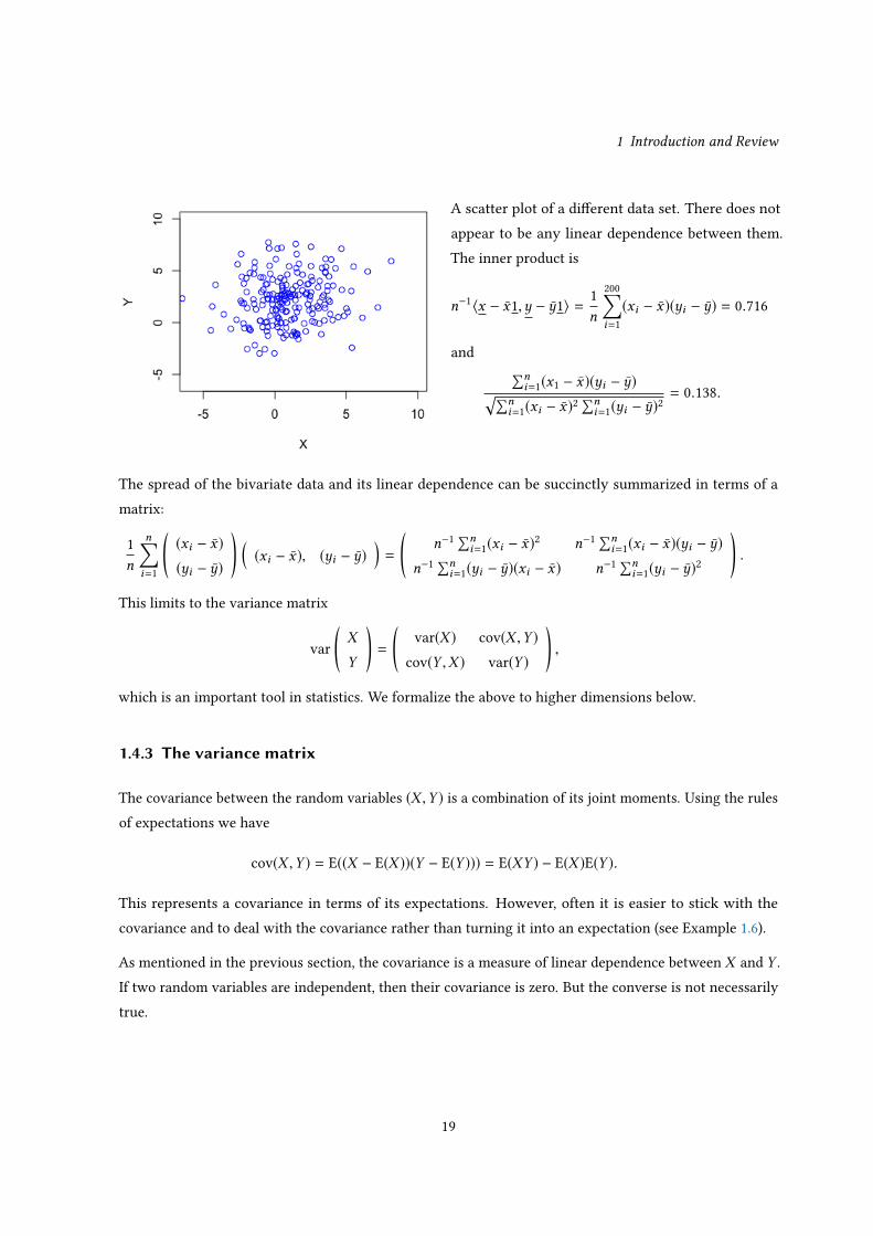
A scatter plot of a di�erent data set. There does notappear to be any linear dependence between them.The inner product is

n

�1hx � x1,� � �1i = 1n

200’i=1

(xi � x)(�i � �) = 0.716

and Õni=1(x1 � x)(�i � �)pÕn

i=1(xi � x)2 Õni=1(�i � �)2

= 0.138.

The spread of the bivariate data and its linear dependence can be succinctly summarized in terms of amatrix:

1n

n’i=1

(xi � x)(�i � �)

! ⇣(xi � x), (�i � �)

⌘=

n

�1 Õni=1(xi � x)2 n

�1 Õni=1(xi � x)(�i � �)

n

�1 Õni=1(�i � �)(xi � x) n

�1 Õni=1(�i � �)2

!.

This limits to the variance matrix

var

X

Y

!=

var(X ) cov(X ,Y )

cov(Y ,X ) var(Y )

!,

which is an important tool in statistics. We formalize the above to higher dimensions below.

1.4.3 The variance matrix

The covariance between the random variables (X ,Y ) is a combination of its joint moments. Using the rulesof expectations we have

cov(X ,Y ) = E((X � E(X ))(Y � E(Y ))) = E(XY ) � E(X )E(Y ).

This represents a covariance in terms of its expectations. However, often it is easier to stick with thecovariance and to deal with the covariance rather than turning it into an expectation (see Example 1.6).

As mentioned in the previous section, the covariance is a measure of linear dependence between X and Y .If two random variables are independent, then their covariance is zero. But the converse is not necessarilytrue.

19

1 Introduction and ReviewExample 1.5. Suppose X ,Y ,Z are zero mean independent random variables. De�ne the variablesU1 = ZX

andU2 = ZY , clearly they are dependent. However,

cov(U1,U2) = 0.

See HW1.

The variance is a special case of the covariance

cov(X ,X ) = var(X ) = E(X � E(X ))2 = E(X 2) � E(X )2.

Generalising the above to matrices, the variance of the vector X = (X1, . . . ,Xd ) is the pairwise covariancebetween each element in the vector

var(X ) = E�(X � E(X ))(X � E(X ))0

�=

©≠≠≠≠≠≠´

var(X1) cov(X1,X2) . . . cov(X1,Xd )cov(X2,X1) var(X2) . . . cov(X2,Xd )

......

. . ....

cov(Xd ,X1) cov(Xd ,X2) . . . var(Xd )

™ÆÆÆÆÆÆ¨.

Clearly var(X ) is a square symmetric matrix: since

cov(Xi ,X j ) = E((Xi � E(Xi ))(X j � E(X j ))) = cov(X j ,Xi ).

In general we can de�ne the covariance between two vectors as follows. Suppose X = (X1, . . . ,Xp ) andY = (Y1, . . . ,Yq). Then cov(X ,Y ) is a (p ⇥ q)-matrix where

cov(X ,Y ) =

©≠≠≠≠≠≠´

cov(X1,Y1) cov(X1,Y2) . . . cov(X1,Yq)cov(X2,Y1) cov(X2,Y2) . . . cov(X2,Yq)

......

. . ....

cov(Xp ,Y1) cov(Xp ,Y2) . . . cov(Xp ,Yq)

™ÆÆÆÆÆÆ¨.

Example 1.6. (i) SupposeU ,V ,W are iid random variables with mean zero and variance one. De�ne the

random vector

X =©≠≠≠´

X1

X2

X3

™ÆÆÆ¨=

©≠≠≠´

2U +VV +W

3W

™ÆÆÆ¨.

The expectation of X is E[X ] = (0, 0, 0)0 and pairwise covariance is

var(X1) = cov(2U +V , 2U +V ) = cov(2U , 2U ) + cov(2U ,V ) + cov(V , 2U ) + cov(V ,V )

= 4var(U ) + 4cov(U ,V ) + var(U ) = 4 + 4 ⇥ 0 + 1 = 5

cov(X1,X2) = cov(2U +V ,V +W ) = cov(2U ,V ) + cov(2U ,W ) + cov(V ,W ) + cov(V ,V ) = var(V ) = 1.

20

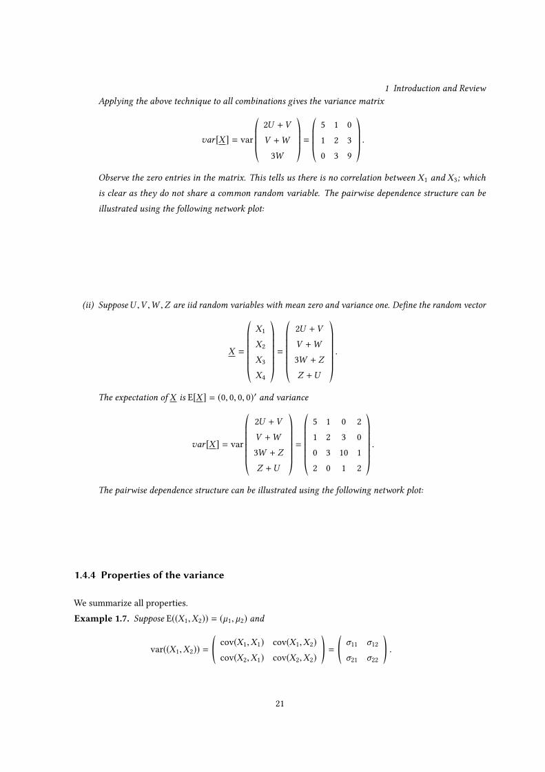
1 Introduction and ReviewApplying the above technique to all combinations gives the variance matrix

�ar [X ] = var©≠≠≠´

2U +VV +W

3W

™ÆÆÆ¨=

©≠≠≠´

5 1 01 2 30 3 9

™ÆÆÆ¨.

Observe the zero entries in the matrix. This tells us there is no correlation between X1 and X3; which

is clear as they do not share a common random variable. The pairwise dependence structure can be

illustrated using the following network plot:

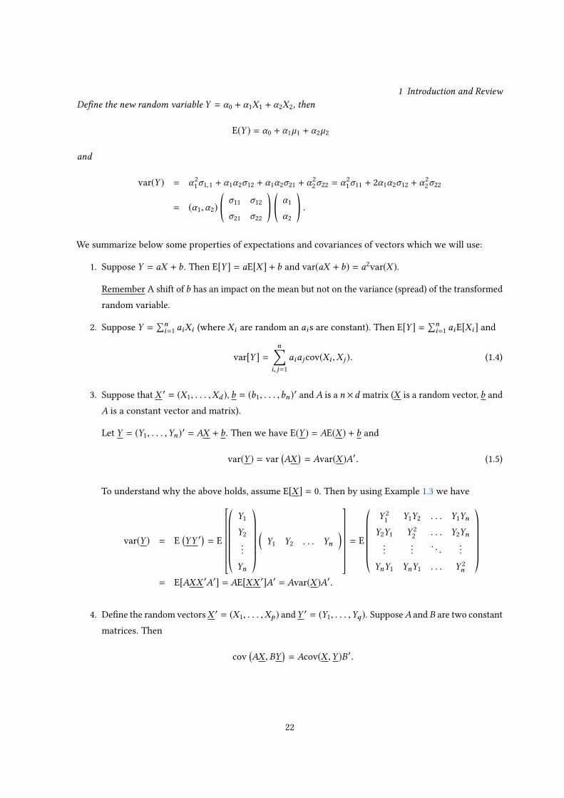
(ii) SupposeU ,V ,W ,Z are iid random variables with mean zero and variance one. De�ne the random vector

X =

©≠≠≠≠≠≠´

X1

X2

X3

X4

™ÆÆÆÆÆÆ¨=

©≠≠≠≠≠≠´

2U +VV +W

3W + ZZ +U

™ÆÆÆÆÆÆ¨.

The expectation of X is E[X ] = (0, 0, 0, 0)0 and variance

�ar [X ] = var

©≠≠≠≠≠≠´

2U +VV +W

3W + ZZ +U

™ÆÆÆÆÆÆ¨=

©≠≠≠≠≠≠´

5 1 0 21 2 3 00 3 10 12 0 1 2

™ÆÆÆÆÆÆ¨.

The pairwise dependence structure can be illustrated using the following network plot:

1.4.4 Properties of the variance

We summarize all properties.Example 1.7. Suppose E((X1,X2)) = (µ1, µ2) and

var((X1,X2)) = cov(X1,X1) cov(X1,X2)cov(X2,X1) cov(X2,X2)

!=

�11 �12

�21 �22

!.

21

1 Introduction and ReviewDe�ne the new random variable Y = �0 + �1X1 + �2X2, then

E(Y ) = �0 + �1µ1 + �2µ2

and

var(Y ) = �

21�1,1 + �1�2�12 + �1�2�21 + �

22�22 = �

21�11 + 2�1�2�12 + �

22�22

= (�1,�2) �11 �12

�21 �22

! �1

�2

!.

We summarize below some properties of expectations and covariances of vectors which we will use:

1. Suppose Y = aX + b. Then E[Y ] = aE[X ] + b and var(aX + b) = a

2var(X ).

Remember A shift of b has an impact on the mean but not on the variance (spread) of the transformedrandom variable.

2. Suppose Y =Õn

i=1 aiXi (where Xi are random an ais are constant). Then E[Y ] = Õni=1 aiE[Xi ] and

var[Y ] =n’

i, j=1aiajcov(Xi ,X j ). (1.4)

3. Suppose that X 0 = (X1, . . . ,Xd ), b = (b1, . . . ,bn)0 and A is a n ⇥d matrix (X is a random vector, b andA is a constant vector and matrix).

Let Y = (Y1, . . . ,Yn)0 = AX + b. Then we have E(Y ) = AE(X ) + b and

var(Y ) = var�AX

�= Avar(X )A0. (1.5)

To understand why the above holds, assume E[X ] = 0. Then by using Example 1.3 we have

var(Y ) = E�YY

0� = E

26666666664

©≠≠≠≠≠≠´

Y1

Y2...

Yn

™ÆÆÆÆÆÆ¨

⇣Y1 Y2 . . . Yn

⌘37777777775= E

©≠≠≠≠≠≠´

Y

21 Y1Y2 . . . Y1Yn

Y2Y1 Y

22 . . . Y2Yn

......

. . ....

YnY1 YnY1 . . . Y

2n

™ÆÆÆÆÆÆ¨

= E[AXX 0A

0] = AE[XX 0]A0 = Avar(X )A0.

4. De�ne the random vectorsX 0 = (X1, . . . ,Xp ) andY 0 = (Y1, . . . ,Yq). SupposeA and B are two constantmatrices. Then

cov�AX ,BY

�= Acov(X ,Y )B0.

22

1 Introduction and ReviewExample 1.8. [The sample mean]

De�ne

Xn = n�1(X1 + . . . + Xn).

Suppose that {Xi } are iid random variables with mean µ and variance � 2. Then we have

E(Xn) = n�1[E(X1) + . . . + E(Xn)] = µ .

And the variance is

var(Xn) = cov

n

�1n’i=1

Xi ,n�1

n’i=1

Xi

!

= n

�2n’

i1,i2=1cov(Xi1 ,Xi2)| {z }=0 if i1,i2

= n�2n’i=1

var(Xi ) =�

2

n

.

Note the above can be shown by using rules of variances of sums (1.4). Alternatively for those who like matrices

we observe that

Xn = (1/n, 1/n, . . . , 1/n)Xn = n�11Xn ,

where X 0n = (X1, . . . ,Xn). Then by using (1.5) we have

var(Xn) = (1/n, 1/n, . . . , 1/n)var(Xn)©≠≠≠´

1/n...

1/n

™ÆÆÆ¨= n�21var(Xn)10.

By expanding out we can see that 1var(Xn)10 is the sum of all entries in matrix var(Xn)

1var(Xn)10 =n’

i1,i2=1cov(Xi1 ,Xi2) =

n’i=1

var(Xi ).

This gives an alternative derivation for the same result. They are both the same, choose the method which suits

you best.

Observe where we required the assumption of independence. We required the assumption of independence (or at

least no correlation) to set cov(Xi1 ,Xi2) = 0 when i1 , i2. If there is dependence, this may not hold (see HW1)!

1.5 Modes of convergence

Convergence of the sample mean is a complex idea, and there are several ways of measuring it. In thissection we review some standard measures.

23

1 Introduction and ReviewBut why do we care? Convergence matters, because we never (rarely; an exception is the 2020 census)observe the population, we can never observe the population parameter. We can only come up with someestimator of it based on a sample. But how do we know this estimator is any good? That it even gets “close”to the true parameter for a very large sample size. To answer this question we need to study di�erent modesof convergence. In this section, we focus on the sample mean (as you would have studied it in previousclasses). In subsequent chapters we consider more sophisticated estimators, but the basic ideas are the same(indeed most estimator can be written as a type of sample mean).

First recall that sample mean is

Xn =1n

n’i=1

Xi

where we assume that {Xi } are iid random variables with mean µ and variance � 2. It can be shown withthe exception of the most extraordinary situations (by extraordinary we mean a set which has measurezero, it rarely happens), Xn ! µ, this is called almost sure convergence. This means as the sample sizegrow it will get closer and closer to the population mean µ. Though useful, it is not very informative.

To illustrate the ideas in this section we consider a running example. We simulate from an chi-squaredistribution (we de�ne this formally in the next chapter, however, the type of distribution does not impactthe discussion in this section) with one degree of freedom, this means E(X ) = µ = 1 and var(X ) = �

2 = 2.For the sample sizes n = 1, . . . , 500 we evaluate the sample mean. Thus for each realisation, we have atrajectory of the sample means from n = 1 to n = 500. In Figure 1.4 we give a plot of �ve trajectories; eachcoloured line corresponds to a speci�c j where

x j,n =1n

n’i=1

x j,i n = 1, . . . , 500

We observe that each trajectory appears to approach one as n grows. Keep in mind, for a given data set{x j,i }ni=1, we can only observe one x j,n = n�1

Õni=1 x j,i (for example, for the sample size n = 20, it may be

the red curve at n = 20). Since µ is unknown), we do not know how close x j,n is µ. In practice we will neverknow the di�erence (x j,n � µ). But there are various ways of measuring the “typical” behaviour of Xn . Wedescribe them in the sections below.

1.5.1 The mean squared error

One measure is the mean squared distance. By mean squared error we mean the average squared distancebetween each trajectory (for a �xed n) and the mean µ, where the average is taken over all possiblerealisations. In Figure 1.5 we give the trajectories of 100 realisations (from n = 1, . . . , 500), we denote eachrealisation as x j,n = n�1

Õni=1 xi, j . An estimate the mean squared error at sample size n we calculate:

24


Figure 1.4: Trajectories of �ve di�erent sample means for sample sizes n=1,. . . ,500.

Figure 1.5: 100 di�erent trajectories for sample sizes n=1,. . . ,100. In red is the standard errorp2/n of the

sample mean.

1100

100’i=1

(x j,n � µ)2,

where xi,n denotes the jth trajectory of the plot at sample size n and µ = 1. A plot of these average squarederror is given in Figure 1.6 However, the true mean squared error should be over all realisations. We recall,

25


Figure 1.6: The average squared error evaluated over 100 di�erent realisations (dots and red) and the meansquared error 2/100 (blue).

that this is simply the expectation of the squared di�erence (Xn � µ):

E�Xn � µ

�2.

By simply expanding the expectation it can be shown that

E�Xn � µ

�2= E

�Xn � E(Xn) + E(Xn) � µ

�2= E

�Xn � E(Xn)

�2+ 2 E

�Xn � E(Xn)

�| {z }

=0

E�E(Xn) � µ

�+ E

�E(Xn) � µ

�2

= E�Xn � E(Xn

�2+

�E(Xn) � µ

�2= var(Xn)| {z }

variance

+�E(Xn) � µ

�2.| {z }

bias squared

(1.6)

This is the “classical” decomposition of the mean squared error of an estimator in terms of its variance andits bias squared.De�nition 1.6 (Bias and standard error). Suppose b

�n is an estimator of a parameter � . The bias of b�n is

de�ned as

B� (b�n) = (E[b�n] � � )

and the standard error de�ned as the square root of the variance of the estimator:

s .e(b�n) =qvar(b�n).

26

1 Introduction and ReviewThe mean squared error is

E⇣b�n � �

⌘2= var(b�n) + B� (b�n)2.

We proved the above mean square error decomposition in (1.6).

For our example, where we consider the sample mean E(Xn) = µ (see Example 1.8), the bias is zero for allsample sizes and E

�Xn � µ

�2= var(Xn) = �

2/n (also from Example 1.8). The the average squared errorsgiven in Figure 1.6 is a good approximation of 2/n (since � 2 = 2); compare the red and blue lines. Tosummarise, the mean squared error gives the average squared distance from the estimator to the populationparameter. It is not an asymptotic result, i.e. it holds for any sample size. However, it does not give anyguarantees on the proportion of realisations which are within, say two standard errors (square root ofthe MSE if the bias is zero) of the population parameter. For that we need to know the distribution of theestimator. But �rst we describe convergence in probability.

1.5.2 Convergence in probability

Convergence in probability is evaluated at every n. Roughly speaking it is the “proportion” of trajectoriesXn , at sample size n, which deviates from µ by more than � . If this proportion converges to zero for every �as n ! 1, then the estimator converges in probability to µ. Formally, if for every � > 0 we have

P(|Xn � µ | > �) ! 0

as n ! 1. Then we say XnP! µ as n ! 1.

Convergence in probability is a weaker form of convergence than almost sure convergence and convergencein mean square. This means almost sure convergence and convergence in mean square imply convergencein probability, but the converse is not true. Though this is very important, it is something that we do notworry too much about in this class. But we should keep in mind that there exists strange examples, whereconvergence in probability can occur but not almost sure convergence. That is, examples where, as n grows,collectively the group of trajectories become tightly gathered about the µ (increasingly bunched together).But individually, many trajectory on an in�nite number of occasions deviates far from µ. Thus, individuallythese trajectories do not converge to µ (so no almost sure convergence). It is di�cult to illustrate. But wemake an attempt in Figure 1.7; we observe that in general all the trajectories are congregating about themean, µ = 1, but there are excursions; each individually trajectory is not converging to µ = 1.

1.5.3 Sampling distributions and the central limit theorem

We return to the trajectories in Figure 1.5. For sample sizes n = 1, 5, 10 and 100 we make a histogram of

X andpn

(Xn � µ)�

27


Figure 1.7: Trajectories of �ve sample means (observe the individual excursions away from one).

together with a QQplot ofpn

(Xn�µ)� against the quantiles of a standard normal distribution. The reason we

consider the “z-transform”pn

(Xn�µ)� (recall we make this transform when looking up the z-tables) is that it

mean zero and variance one (it standardizes Xn). This is is similar to taking a cross section across Figure1.5 n = 1, 5, 10 and 100 and studying the distribution of the trajectories at each of these intersections. Theplots are given in Figures 1.8 - 1.11.

n=1

sample size

0 1 2 3 4 5 6

010

2030

4050

6070

n=1

sample size

−1 0 1 2 3 4

010

2030

40

−2 −1 0 1 2

−0.5

0.00.5

1.01.5

2.02.5

normal quantiles

quan

tiles o

f sam

ple m

ean

Figure 1.8: Sample size n = 1. Histogram of X , (X � 1)/p2 and the QQplot against a standard normal

distribution. Using 100 replications.

28

1 Introduction and Reviewn=5

sample size

0 1 2 3 4 5 6

010

2030

40n=5

sample size

−1 0 1 2 3

05

1015

2025

30

−2 −1 0 1 2

−10

12

3

normal quantiles

quan

tiles o

f sam

ple m

ean

Figure 1.9: Sample size n = 5. Histogram of X5,p5(X5 � 1)/

p2 and the QQplot against a standard normal

distribution. Using 100 replications.

n=10

sample size

0 1 2 3 4 5 6

010

2030

40

n=10

sample size

−2 −1 0 1 2 3

05

1015

20

−2 −1 0 1 2

−10

12

normal quantiles

quan

tiles o

f sam

ple m

ean


p2 and the QQplot against a standard

normal distribution. Using 100 replications.

n=100

sample size

0 1 2 3 4 5 6

05

1015

2025

30

n=100

sample size

−3 −2 −1 0 1 2 3

010

2030

−2 −1 0 1 2

−2−1

01

2

normal quantiles

quan

tiles o

f sam

ple m

ean


p2 and the QQplot against a standard

normal distribution. Using 100 replications.

De�nition 1.7 (Sampling distribution of an estimator). The distribution of an estimator is called the sampling

distribution of the estimator. For the Xn described in our running sample, the sampling distribution of Xn are

29

1 Introduction and Reviewthe histograms given in Figures 1.8-1.11.

De�nition 1.8 (Quantile Quantile plot). A Quantile Quantile plot (QQplot for short) is a useful method for

checking if the data can plausibly come from a conjectured distribution. It plots the ordered data against the

corresponding quantiles of the corresponding distribution. In Figure 1.8-1.11, we have plotted ordered sample

means (for a given sample size) against the quantiles of a standard normal distribution.

More precisely, suppose we observe the data Y1,Y2, . . . ,Yn (these could be raw data or several averages, as given

in this example). We order the data from the smallest number to the largest, often denotedY(1,n),Y(2,n), . . . ,Y(n,n).

If {Yi } came from a standard normal distribution we would expect the median of the data, Y(n/2,n) to closely

match the 50% (median) quantile in the standard normal distribution (which is zero). Similarly, we would

expect Y(n/4,n) to close match the �rst quartile of a standard normal (which is -0.674, you can get these numbers

from the z-tables) and Y(3n/4,n) to close match the third quartile of a standard normal (which is 0.674).

Extending this argument, we would expect thatY(i,n) roughly matches the quantile corresponding the probability

i/n in the normal distribution. Based on this argument, we de�ne the n quantiles in a standard normal

distribution. Let zi,n be such that

P(Z zi,n) =(i � 0.5)

n

,

where Z is a standard normal distribution (mean zero and variance one). We subtract use (i � 0.5)/n rather

than i/n to avoid the case P(Z zn,n) = 1 (when i = n). {zi,n} are called the standard normal quantiles (you

can �nd them in the z-tables). A standard normal QQplot is a plot of {(zi,n ,Y(i,n))}ni=1. The line is usually (but

not always) the line corresponding to (zi,n , zi,n). If the data is normal, it will the QQplot will lie close to the line.

In R, the function qqplot plots the data against the quantiles of the normal distribution whose mean and

variance are the sample mean and variance calculated from the data. The function qqlines makes a line which

goes through the 25th and 75th quantiles of the standard normal distribution and corresponding data.

Studying the plots from n = 1, 5, 10 and 100 we �rst observe that the histogram of the �rst plot becomesnarrower as the sample size grows (this corresponds to the trajectories in Figure 1.5 getting increasinglybunched together). This is because the standard error �/pn gets smaller as the sample size grows. Further,the histograms tend to resemble a normal distribution as the sample size grow. Observe further, as thesample size grow the quantiles of standardized sample mean match well the quantiles of the standardnormal distribution. This is called the central limit theorem, and we state this formally below. We mentionthat in our example, the distribution of the original data {Xi } is skewed (see the plot in Figure 1.8, which isthe histogram of Xi , since the sample size is n = 1). The skew in the original distribution means that ittakes a larger sample size for the samling distribution of the sample mean to be close to normal. Observethat when n = 10, evidence of a skew is still seen in the QQplot, but it is no longer so evident for n = 100.

We state the central limit theorem in its simplest form.

30


Theorem 1.1

Suppose that {Xi } are iid random variables with mean µ and variance �

2 (a �nite variance is anecessary condition). Let

Xn =1n

n’i=1

Xi .

Using the results in Section 1.4.1 we have

E(Xn) =1n

n’i=1

E(Xi ) = µ and var(Xn) =�

2

n

.

Then

pn

�Xn � µ

� D! N(0,� 2) n ! 1.

This means that the density (or histogram) associated with the random variablepn

�Xn � µ

�gets more and

more standard normal looking as the number of Xis used to construct the Xn increase. By dividing by �and using the results in Section 1.4.1 we have

Ep

n

�Xn � µ

��

�= 0 �ar

pn

�Xn � µ

��

�= 1

andpn

�Xn � µ

��

D! N (0, 1)

as n ! 1. Alternatively, if we want to apply the above results, then we can write the above result as

XnD! N

✓µ,

�

2

n

◆.

This way of writing the result corresponds to the left hand side histogram in Figures 1.8-1.11.

However, the actual sample size required for the normal approximation to hold well depends on thecharacteristics of the distribution of Xi . The factor that plays the largest role is the skewness (asymmetry)of the original distribution. The greater the level of asymmetry in the density or pmf of Xi , the larger thesample size required for the normal approximation to hold. This e�ect is easily seen in simulations. Further,as can be seen from the QQplots, the deviance between the distribution of the sample mean and normaldistribution di�ers greatest in the tails. The asymmetric is measured using skewness, which we de�ne inthe section below.

De�nition 1.9 (Summary of di�erent modes of convergence). (i) Almost sure convergence. This is where

all the trajectories (except for the really weird and exceptional ones) converge to the mean, µ. In some

sense this is the easiest to understand. We often denote this as Xna .s .! µ.

31

1 Introduction and Review(ii) Mean squared convergence. This is essentially the average square distance between the trajectory (at

sample size n) and µ. If the estimator converges in mean square then E(Xn � µ)2 ! 0 as n ! 1.

(iii) Convergence in probability: If for every � > 0 we have

P(|Xn � µ | > �) ! 0

as n ! 1. Then we say XnP! µ as n ! 1.

(iv) Convergence in distribution: we may write

pn

�Xn � µ

��

D! N(0, 1)

orpn

�Xn � µ

�/� D! Z , where Z is a standard normal random variable.

Skewness: Measure of asymmetry

Skewness is usually de�ned using the third moment

S3 =E(Xi � µ)3

�

3

To understand why this measure asymmetry assume µ = 0 (without loss of generality). It is easily seen ifthe the distribution is symmetric about the mean, then S3 = 0;

E(X 3) =π 1

�1x

3f (x)dx =

π 1

0x

3f (x)dx +

π 0

�1x

3f (x)dx

=

π 1

�1x

3f (x)dx =

π 1

0x

3f (x)dx +

π 0

�1x

3f (�x)dx (change variables x = ��)

=

π 1

�1x

3f (x)dx =

π 1

0x

3f (x)dx �

π 1

0�

3f (�)d� = 0,

essentially the positives in (Xi � µ)3 cancel with the negatives (this is best seen with a picture). If thedistribution is not symmetric then this cancellation may not be possible and S3 may not be zero. It can beshown that the size of |S3 | together with the sample size e�ects the quality of the normal approximation ofthe distribution of the sample mean. For the �

2 distribution withm-df (we de�ne it formally in the nextchapter), S3 =

p8/m. Observe that the level of skewness decreases asm grows.

Suppose we observe the iid random variables {Xi }ni=1, we can estimate E(X � µ)3 with the centralizedaverage

µ3 = n�1

n’i=1

(Xi � X )3

and the variance � 2 with

b� 2 = n�1n’i=1

(Xi � X )2.

32

1 Introduction and ReviewThis gives an estimator of S3

bS3 =

n

�1 Õni=1(Xi � X )3

b� 3n

.

1.5.4 Functions of sample means

In statistics many estimators we encounter are averages or functions of averages. Suppose XnP! µ and

pn(Xn � µ) D! N (0,� 2), what happens to X 2

n? By the continuous mapping theorem

X

2n

P! µ

2.

Further, if µ , 0, then

pn(X 2

n � µ

2) D! N (0, 4µ2� 2)

as n ! 1.

In general, we have the following result (usually called the continuous mapping theorem).

Lemma 1.2

Suppose XnP! µ as n ! 1 and � is a continuous function, then

�(Xn)P! �(µ),

as n ! 1. Furthermore, ifpn(Xn � µ) D! N (0,� 2) and �0(µ) , 0 then we have

pn[�(Xn) � �(µ)] D! N (0, [�0(µ)]2� 2) (1.7)

as n ! 1.

PROOF. The proof is beyond this course, but a rough outline of the normality result is given below. Thesecond order mean value theorem of �(Xn) about �(µ) gives

�(Xn) � �(µ) = (Xn � µ)�0(µ) + 12(Xn � µ)2�00(�µ + (1 � �)Xn).

Since XnP! µ, (Xn � µ)2 << ((Xn � µ)); thus the �rst term of the RHS of the above “dominates” the second

term and we have

�(Xn) � �(µ) ⇡ (Xn � µ)�0(µ).

Note this is why we require �0(µ) , 0. Since we have asymptotic normality of (Xn � µ) and �

0(µ) is aconstant, we have the result. ⇤

33

1 Introduction and ReviewThis result turns out to be very useful in many of the methods we discuss in the subsequent chapters.

To illustrate the result, in Figures 1.12 and 1.13 we give a plot of the histogram of X 2n (for two di�erent

sample sizes n = 200 and 1000, conducted over 1000 replications) in the case that µ = 0 and µ = 0.5. Werecall that �0(µ) = 2µ) and that for (1.7) to hold, we require �0(µ) , 0. If this condition is violated, as isthe case that µ = 0, then this result does not hold. This is clearly seen in Figure 1.12, for both the samplesizes n = 200 and n = 1000, the distributions is clearly not normal. On the other hand, when µ = 0.5, then

Figure 1.12: The histogram of X 2n when µ = 0: Left n = 200, Right: n = 1000.

�

0(0.5) , 0, thus (1.7) should hold when n is large. In Figure 1.13 we see that this is indeed the case. Forn = 200, there appears to be a small right skew, which appears to have almost diminished when n = 1000.This essentially illustrates the power of (1.7); a transformation of the sample mean is also asymptoticallynormal, so long as �0(µ) ,= 0.Example 1.9 (Transformations to reduce skewness). In a simulation, I draw from a Poisson with � = 0.5, 5times and evaluate the sample mean (this is done several times). The histogram for the distribution of X5 is

the top plot in Figure 1.14. Observe the huge skew. We now take a power transform; X �5 using � = 1/2. The

histogram of the lower plot in Figure 1.14. Observe that after taking the square root of the sample mean, it is

normal looking. I found that taking a square root is a lot better than taking a cube root. This is a neat trick for

making estimators more normal in their distribution. Note that from Lemma 1.2 we have

pn(X 1/2

n � �

1/2) D! N

⇣0, � ⇥ [��1/2/2]2

⌘.

The above can be generalized to functions of several averages. Suppose {Xi } and {Yi } are iid random

34


Figure 1.13: The histogram of X 2n when µ = 0.5: Left n = 200, Right: n = 1000.

Figure 1.14: Top plot histogram of X5. Lower plot histogram of X 1/2n .

35

1 Introduction and Reviewvariables with mean µX and µY (respectively) and variance

� =

�ar (X ) cov(X ,Y )cov(Y ,X ) var(Y )

!.

Let Xn = n�1 Õn

i=1Xi and Yn = n�1Õn

i=1 Yi . Suppose the multivariate CLT holds (see STAT414, for details)such that

pn

Xn � µX

Yn � µY

!D! N (0, �) .

Let Zn = �(Xn , Yn), where Xn = n�1 Õn

i=1Xi and Yn = n�1Õn

i=1 Yi . If

�(µ1, µ2) =✓@�(x ,�)@x

,@�(x ,�)@�

◆c(x=µx ,�=µ� ) , 0,

then we have

pn

��(Xn , Yn) � �(µX , µY )

� D! N⇣0,�(µX , µY )��(µX , µY )0

⌘.

Research 1. Run some simulations for di�erent functions of averages. Plot the histogram and calculate the

standard deviations in the simulations. Do they match the results given above for su�ciently large n?

1.6 A historical perspective

The Central Limit Theorem dates back to Laplace in 1810. In 1824, Poisson gave a more rigourous proof ofthe result. However, the �rst rigourous version of the proof was established by Lyapunouv in 1901. In 1922Lindeburg, established the result under the weaker condition that only the �rst and second moments of therandom variable are �nite (this turns out to be su�cient and necessary condition).

36

Mathematical Statistics II: Demystifying statisticssuhasini/teaching415/chapter1.pdf ·...

Documents

Transcript of Mathematical Statistics II: Demystifying statisticssuhasini/teaching415/chapter1.pdf ·...