Article

Mathematical Models of Androgen Resistance inProstate Cancer Patients under Intermittent AndrogenSuppression Therapy

Javier Baez and Yang Kuang *

School of Mathematical and Statistical Sciences, Arizona State University, Tempe, AZ 85287, USA;jbaez2@asu.edu* Correspondence: kuang@asu.edu; Tel.: +1-480-965-6915

Academic Editor: Serafim KalliadasisReceived: 15 August 2016; Accepted: 5 November 2016; Published: 16 November 2016

Abstract: Predicting the timing of a castrate resistant prostate cancer is critical to loweringmedical costs and improving the quality of life of advanced prostate cancer patients. We formulate,compare and analyze two mathematical models that aim to forecast future levels of prostate-specificantigen (PSA). We accomplish these tasks by employing clinical data of locally advanced prostate cancerpatients undergoing androgen deprivation therapy (ADT). While these models are simplifications ofa previously published model, they fit data with similar accuracy and improve forecasting results.Both models describe the progression of androgen resistance. Although Model 1 is simpler thanthe more realistic Model 2, it can fit clinical data to a greater precision. However, we found thatModel 2 can forecast future PSA levels more accurately. These findings suggest that including morerealistic mechanisms of androgen dynamics in a two population model may help androgen resistancetiming prediction.

Keywords: mathematical modeling; prostate cancer; androgen deprivation therapy; data fitting

1. Introduction

Ever since the discovery of androgen dependency of prostate cells, androgen deprivation therapy(ADT) has played a vital role in the treatment of metastatic and locally advanced prostate cancer [1–3].However, controversy remains regarding its best application. Although this treatment will regresstumors in over 90% of patients [4], after prolonged androgen depletion, patients will eventuallydevelop castration-resistant prostate cancer (CRPC) [5]. The development of CRPC can take froma few months to more than ten years [3,6], after which there is a very limited number of effectivetreatments and patients suffer high mortality [7]. ADT is expensive and its side effects include sexualdysfunction, hot flashes, and fatigue [8]. Based on some preclinical studies, intermittent androgensuppression (IAS) is suggested as a sensible alternative to ADT [9]. During off-treatment periods,patients enjoy a “vacation” from the severe side effects of ADT [8], and studies have suggested thatIAS may not negatively affect the time to resistance progression or survival in comparison to ADT [10].Consequently, IAS is selected by some patients to improve the quality of life and also hopefully todelay the progression to CRPC [4].

Many mathematical models have studied the dynamics of prostate cancer during ADT orIAS [11–18]. A detailed review of some of these models are presented in the recent book ofKuang et al. [19]. Ideta et al. are pioneers of mathematically modeling and analyzing the dynamicsof IAS [12]. They formulated a system of ordinary differential equations to study the mechanics ofADT and IAS. They considered castrate-resistant (CR) and castrate-sensitive (CS) cell populations aswell as androgen levels. Their model included mutations from CS to CR cells, and their focus was on

Appl. Sci. 2016, 6, 352; doi:10.3390/app6110352 www.mdpi.com/journal/applsci

Appl. Sci. 2016, 6, 352 2 of 16

comparing continuous and intermittent therapy and the development of resistance. Hirata et al. [14]introduced a piece-wise linear model of three cancer cell populations. Their model included CS cells,CR cells that may mutate into CS cells, and CR cells that will not mutate. Several investigators usingHirata et al.’s model [14] have studied estimation of parameters [20,21], optimal switching times andcontrol in IAS [20,22,23], and forecasting CRPC progression [24,25].

Built on the works of Ideta et al. [12] and Jackson [26], Portz, Kuang, and Nagy (PKN) [13] developeda novel mathematical model to study the dynamics of IAS by using the cell quota model [27] frommathematical ecology, which relates growth rate to an intracellular nutrient, to modeling the growthof both the CS and CR cell populations. The cell quota in [13] is defined as the intracellular androgenconcentrations for each cell population. This model is carefully fitted with clinical prostate-specificantigen (PSA) data, where androgen data was used to model the cell quota and other growthparameters. Everett et al. [28] compared the models of Hirata et al. [14] and PKN [13] regardingtheir accuracy of fitting clinical data and predicting future PSA levels. They concluded that whilea biologically-based model is important to reveal the underlying processes and my present more robustand better predictions, a simpler model such as that of Hirata et al. might also be practical for fittingclinical data and predicting future PSA outcomes of individual patients.

In this paper, we present a simplified model to the final model in PKN [13]. Several key terms inour model will be mechanistically formulated. This model is concise and amenable to systematicalmathematical analysis of its dynamics. For simplicity, we shall use serum androgen concentration toapproximate intracellular androgen. This is reasonable since androgen passively and quickly diffusesthrough the prostate membrane via concentration gradient [29]. This approach is practical for a typicalclinical setting, where the data collected can be applied directly to the model. Most importantly,our model can fit PSA and androgen values simultaneously, which enables us to be more accurate inmaking future PSA value predictions.

2. Clinical Trial Data

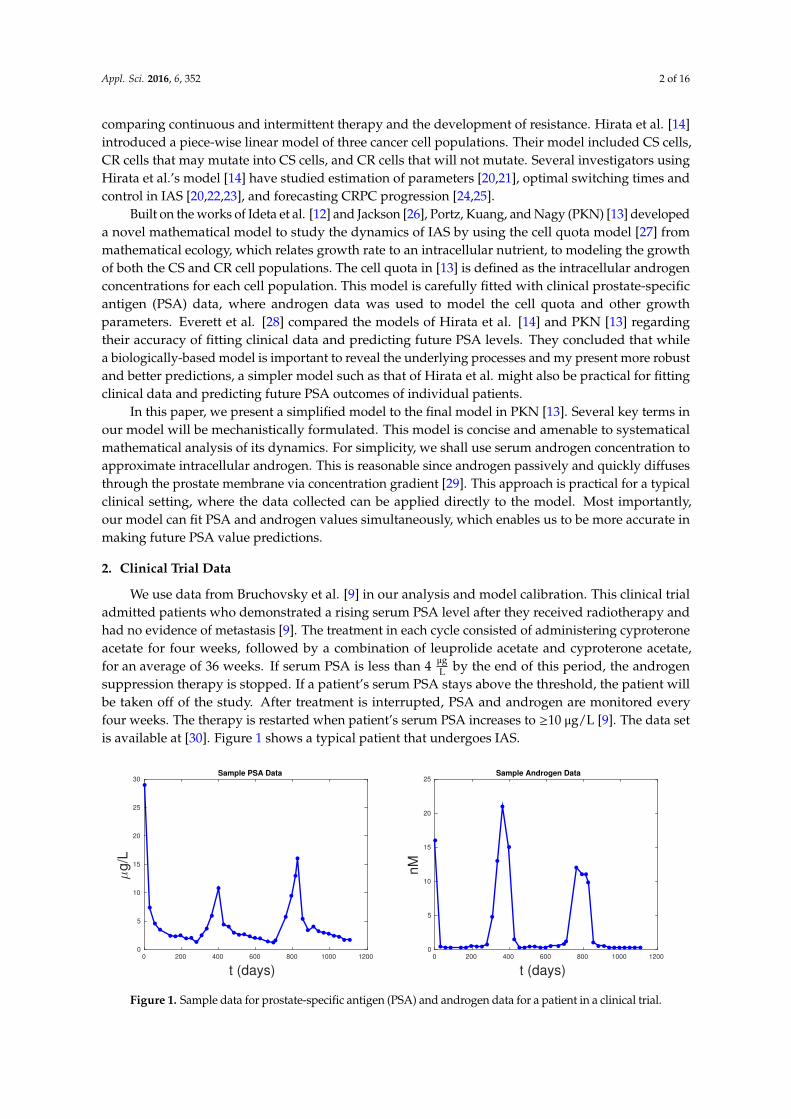
We use data from Bruchovsky et al. [9] in our analysis and model calibration. This clinical trialadmitted patients who demonstrated a rising serum PSA level after they received radiotherapy andhad no evidence of metastasis [9]. The treatment in each cycle consisted of administering cyproteroneacetate for four weeks, followed by a combination of leuprolide acetate and cyproterone acetate,for an average of 36 weeks. If serum PSA is less than 4 µg

L by the end of this period, the androgensuppression therapy is stopped. If a patient’s serum PSA stays above the threshold, the patient willbe taken off of the study. After treatment is interrupted, PSA and androgen are monitored everyfour weeks. The therapy is restarted when patient’s serum PSA increases to ≥10 µg/L [9]. The data setis available at [30]. Figure 1 shows a typical patient that undergoes IAS.

t (days)0 200 400 600 800 1000 1200

µg/L

0

5

10

15

20

25

30Sample PSA Data

t (days)0 200 400 600 800 1000 1200

nM

0

5

10

15

20

25Sample Androgen Data

Figure 1. Sample data for prostate-specific antigen (PSA) and androgen data for a patient in a clinical trial.

Appl. Sci. 2016, 6, 352 3 of 16

3. Formulation of Mathematical Models

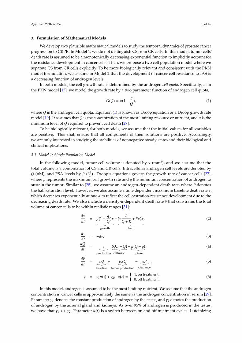
We develop two plausible mathematical models to study the temporal dynamics of prostate cancerprogression to CRPR. In Model 1, we do not distinguish CS from CR cells. In this model, tumor cells’death rate is assumed to be a monotonically decreasing exponential function to implicitly account forthe resistance development in cancer cells. Then, we propose a two cell population model where weseparate CS from CR cells explicitly. To be more biologically relevant and consistent with the PKNmodel formulation, we assume in Model 2 that the development of cancer cell resistance to IAS isa decreasing function of androgen levels.

In both models, the cell growth rate is determined by the androgen cell quota. Specifically, as inthe PKN model [13], we model the growth rate by a two parameter function of androgen cell quota,

G (Q ) = µ (1 −q

Q), (1)

where Q is the androgen cell quota. Equation (1) is known as Droop equation or a Droop growth ratemodel [19]. It assumes that Q is the concentration of the most limiting resource or nutrient, and q is theminimum level of Q required to prevent cell death [27].

To be biologically relevant, for both models, we assume that the initial values for all variablesare positive. This shall ensure that all components of their solutions are positive. Accordingly,we are only interested in studying the stabilities of nonnegative steady states and their biological andclinical implications.

3.1. Model 1: Single Population Model

In the following model, tumor cell volume is denoted by x (mm3), and we assume that thetotal volume is a combination of CS and CR cells. Intracellular androgen cell levels are denoted byQ (nM), and PSA levels by P (

µgL ). Droop’s equations govern the growth rate of cancer cells [27],

where µ represents the maximum cell growth rate and q the minimum concentration of androgen tosustain the tumor. Similar to [28], we assume an androgen-dependent death rate, where R denotesthe half saturation level. However, we also assume a time dependent maximum baseline death rate ν ,which decreases exponentially at rate d to reflect the cell castration-resistance development due to thedecreasing death rate. We also include a density-independent death rate δ that constrains the totalvolume of cancer cells to be within realistic ranges [31]:

dx

dt= µ (1 −

q

Q)x︸ ︷︷ ︸

growth

− (νR

Q + R+ δx )x︸ ︷︷ ︸

death

, (2)

dν

dt= −dν , (3)

dQ

dt= γ︸︷︷︸

production

(Qm −Q )︸ ︷︷ ︸diffusion

− µ (Q − q)︸ ︷︷ ︸uptake

, (4)

dP

dt= bQ︸︷︷︸

baseline

+ σxQ︸︷︷︸tumor production

− ϵP︸︷︷︸clearance

, (5)

γ = γ1u (t ) +γ2, u (t ) =

{1, on treatment,0, off treatment.

(6)

In this model, androgen is assumed to be the most limiting nutrient. We assume that the androgenconcentration in cancer cells is approximately the same as the androgen concentration in serum [29].Parameter γ1 denotes the constant production of androgen by the testes, and γ2 denotes the productionof androgen by the adrenal gland and kidneys. As over 95% of androgen is produced in the testes,we have that γ1 >> γ2. Parameter u (t ) is a switch between on and off treatment cycles. Luteinizing

Appl. Sci. 2016, 6, 352 4 of 16

hormone releasing hormone agonists only stop testes production of androgen during treatment.During treatment, γ2 will be the only production of androgen. Qm > q denotes the maximum androgenlevel in serum. The androgen uptake by prostate cells is assumed to be proportional to the differenceof the maximum possible and the current androgen levels in serum. Androgen in cells is depleted forgrowth at a rate of µ (Q − q). PSA is produced by both the regular cells in the prostate at the rate bQ

and by the cancer cells at the rate σxQ . Notice that we have assumed that cell production of PSA isassumed to be dependent on levels of androgen. Finally, PSA is cleared from serum at rate ϵ .

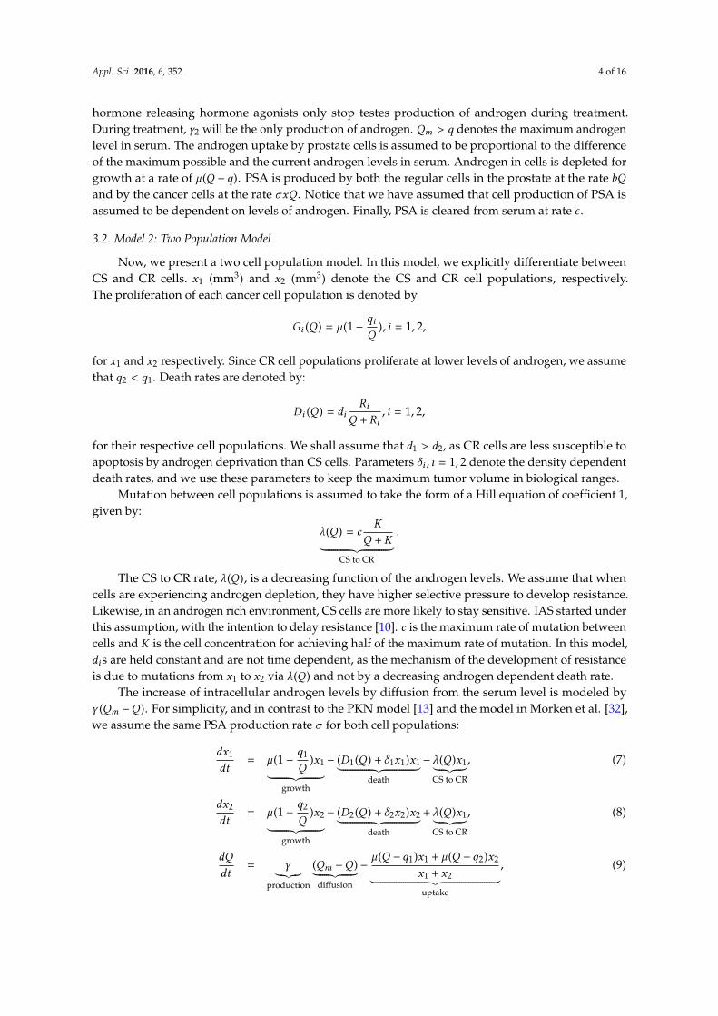
3.2. Model 2: Two Population Model

Now, we present a two cell population model. In this model, we explicitly differentiate betweenCS and CR cells. x1 (mm3) and x2 (mm3) denote the CS and CR cell populations, respectively.The proliferation of each cancer cell population is denoted by

Gi (Q ) = µ (1 −qiQ), i = 1, 2,

for x1 and x2 respectively. Since CR cell populations proliferate at lower levels of androgen, we assumethat q2 < q1. Death rates are denoted by:

Di (Q ) = diRi

Q + Ri, i = 1, 2,

for their respective cell populations. We shall assume that d1 > d2, as CR cells are less susceptible toapoptosis by androgen deprivation than CS cells. Parameters δi , i = 1, 2 denote the density dependentdeath rates, and we use these parameters to keep the maximum tumor volume in biological ranges.

Mutation between cell populations is assumed to take the form of a Hill equation of coefficient 1,given by:

λ(Q ) = cK

Q +K︸ ︷︷ ︸CS to CR

.

The CS to CR rate, λ(Q ), is a decreasing function of the androgen levels. We assume that whencells are experiencing androgen depletion, they have higher selective pressure to develop resistance.Likewise, in an androgen rich environment, CS cells are more likely to stay sensitive. IAS started underthis assumption, with the intention to delay resistance [10]. c is the maximum rate of mutation betweencells and K is the cell concentration for achieving half of the maximum rate of mutation. In this model,dis are held constant and are not time dependent, as the mechanism of the development of resistanceis due to mutations from x1 to x2 via λ(Q ) and not by a decreasing androgen dependent death rate.

The increase of intracellular androgen levels by diffusion from the serum level is modeled byγ (Qm −Q ). For simplicity, and in contrast to the PKN model [13] and the model in Morken et al. [32],we assume the same PSA production rate σ for both cell populations:

dx1

dt= µ (1 −

q1

Q)x1︸ ︷︷ ︸

growth

− (D1 (Q ) + δ1x1)x1︸ ︷︷ ︸death

− λ(Q )x1︸ ︷︷ ︸CS to CR

, (7)

dx2

dt= µ (1 −

q2

Q)x2︸ ︷︷ ︸

growth

− (D2 (Q ) + δ2x2)x2︸ ︷︷ ︸death

+ λ(Q )x1︸ ︷︷ ︸CS to CR

, (8)

dQ

dt= γ︸︷︷︸

production

(Qm −Q )︸ ︷︷ ︸diffusion

−µ (Q − q1)x1 + µ (Q − q2)x2

x1 + x2︸ ︷︷ ︸uptake

, (9)

Appl. Sci. 2016, 6, 352 5 of 16

dP

dt= bQ︸︷︷︸

baseline

+ σ (Qx1 +Qx2)︸ ︷︷ ︸tumor production

− ϵP .︸︷︷︸clearence

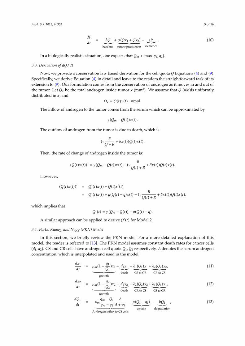
. (10)

In a biologically realistic situation, one expects that Qm > max{q1,q2}.

3.3. Derivation of dQ/dt

Now, we provide a conservation law based derivation for the cell quota Q Equations (4) and (9).Specifically, we derive Equation (4) in detail and leave to the readers the straightforward task of itsextension to (9). Our formulation comes from the conservation of androgen as it moves in and out ofthe tumor. Let Qx be the total androgen inside tumor x (mm3). We assume that Q (nM )is uniformlydistributed in x , and

Qx = Q (t )x (t ) nmol.

The inflow of androgen to the tumor comes from the serum which can be approximated by

γ (Qm −Q (t ))x (t ).

The outflow of androgen from the tumor is due to death, which is

(νR

Q + R+ δx (t ))Q (t )x (t ).

Then, the rate of change of androgen inside the tumor is:

(Q (t )x (t ))′ = γ (Qm −Q (t ))x (t ) − (νR

Q (t ) + R+ δx (t ))Q (t )x (t ).

However,

(Q (t )x (t ))′ = Q ′(t )x (t ) +Q (t )x ′(t )

= Q ′(t )x (t ) + µ (Q (t ) − q)x (t ) − (νR

Q (t ) + R+ δx (t ))Q (t )x (t ),

which implies thatQ ′(t ) = γ (Qm −Q (t )) − µ (Q (t ) − q).

A similar approach can be applied to derive Q ′(t ) for Model 2.

3.4. Portz, Kuang, and Nagy (PKN) Model

In this section, we briefly review the PKN model. For a more detailed explanation of thismodel, the reader is referred to [13]. The PKN model assumes constant death rates for cancer cells(d1,d2). CS and CR cells have androgen cell quota Q1,Q2 respectively. A denotes the serum androgenconcentration, which is interpolated and used in the model:

dx1

dt= µm (1 −

q1

Q1)x1︸ ︷︷ ︸

growth

− d1x1︸︷︷︸death

− λ1 (Q1)x1︸ ︷︷ ︸CS to CR

+ λ2 (Q2)x2︸ ︷︷ ︸CR to CS

, (11)

dx2

dt= µm (1 −

q2

Q2)x2︸ ︷︷ ︸

growth

− d2x2︸︷︷︸death

− λ2 (Q2)x2︸ ︷︷ ︸CR to CS

+ λ1 (Q1)x1︸ ︷︷ ︸CS to CR

, (12)

dQ1

dt= vm

qm −Q1

qm − q1

A

A+vh︸ ︷︷ ︸Androgen influx to CS cells

− µ (Q1 − q1)︸ ︷︷ ︸uptake

− bQ1︸︷︷︸degradation

, (13)

Appl. Sci. 2016, 6, 352 6 of 16

dQ2

dt= vm

qm −Q2

qm − q2

A

A+vh︸ ︷︷ ︸Androgen influx to CR cells

− µ (Q2 − q2)︸ ︷︷ ︸uptake

− bQ2︸︷︷︸degradation

, (14)

dP

dt= σ0 (x1 + x2)︸ ︷︷ ︸

baseline production

+ σ1x1Qm

1

Qm1 + ρ

m1︸ ︷︷ ︸

tumor production

+ σ2x2Qm

2

Qm2 + ρ

m2︸ ︷︷ ︸

tumor production

− δP .︸︷︷︸clearence

. (15)

4. Model Dynamics

Now, we study the mathematical properties and dynamics of our two models. For Model 1,we shall state the results without providing proofs as they are routine. The detailed mathematicalanalysis for Model 2 will be presented. Proposition 1 summarizes the mathematical dynamics ofModel 1. Since P is decoupled from the system, we shall refer only to the dynamics of Equations (2)–(4).This proposition reveals that there is no cure for cancer. Since ADT is non-curative, this property isbiologically reasonable.

Proposition 1. Solutions of the system Equations (2)–(4) are positive and bounded. The system Equations (2)–(4)has a cancer free steady state E0 = (0, 0, γQm+µq

µ+γ ) that is unstable, and a steady state E1 = (µγδ

Qm−qγQm+µq

, 0, γQm+µqµ+γ )

that is globally stable.

Next, we do a thorough mathematical analysis of Model 2. First, we study boundedness andpositivity of the system. Followed by the number and existence of steady states. Finally, we analyzethe local stability of the steady states. Observe that P is also decoupled from Equations (2)–(4) and wedo not include it in the analysis.

Proposition 2. Assume q2 ≤ q1 < Qm and δ1 ≥ δ2. Then, solutions of Equations (7)–(9) with initial conditionsx1 (0) > 0, x2 (0) > 0, and q2 ≤ Q (0) ≤ Qm stay in the region {(x1,x2,Q ) : x1 ≥ 0,x2 ≥ 0,x1 + x2 ≤G2 (Qm )−Dm (q2 )

δ2,q2 ≤ Q ≤ Qm }, where Dm = min{D1 (q2),D2 (q2)}.

Proof. We note that in Equation (7), x1 appears in every term ensuring its positivity. Since x2 appearsin the first two terms of (8) and x1 appears in the last term, the positivity of x2 is also guaranteed.

In addition, q2 ≤ q1 < Qm , and

Q ′ = γ (Qm −Q ) −µ (Q −q1)x1 + µ (Q −q2)x2

x1 + x2.

We see that Q ′(q2) > 0 and Q ′(Qm ) < 0. It is thus easy to see that q2 ≤ Q (t ) ≤ Qm for t > 0 withinitial conditions q2 ≤ Q (0) ≤ Qm .

For boundedness of x1 and x2, we let N = x1 + x2. Since we have that δ1 ≥ δ2, and the growth rateGi (Q ), i = 1, 2 are increasing functions of Q , we have

N ′ ≤ (G2 (Q ) −Dm )N − δ2N2, (16)

≤ (G2 (Qm ) −Dm )N − δ2N2, (17)

which implies that lim supt→∞

N (t ) ≤G2 (Qm ) −Dm

δ2. �

Now, we study the steady states of Model 2. We seek to understand the conditions under whichone population will overtake the other, and the circumstances under which they may coexist.

Proposition 3. Assume q2 ≤ q1 < Qm and δ1 ≥ δ2. The system Equations (7)–(9) have a CR cell onlysteady state E1 = (0, G2 (Q1 )−D2 (Q1 )

δ2,Q1), and a coexistence steady state E2 = (G1 (Q∗ )−D1 (Q∗ )−λ1 (Q∗ )

δ1,x∗2,Q∗),

where Q1 =γQm+µq2

γ+µ and Q∗ > Q1.

Appl. Sci. 2016, 6, 352 7 of 16

Proof. Let E = (x∗1,x∗2,Q∗) be a steady state of the system Equations (7)–(9). We have two mutuallyexclusive cases: x∗1 = 0 and x∗1 > 0.

If x∗1 = 0, then we have two possibilities: (i) x∗2 = 0 or (ii) x∗2 > 0. In the case of (i), we see thatE = E0. In the case of (ii), we see that E = E1.

If x∗1 > 0, we see that x∗2 > 0 from the equation of dx2/dt . In this case, E = E2. In addition, we havethe following:

0 = γ (Qm −Q∗) −

µ (Q∗ −q1)x∗1 + µ (Q

∗ −q2)x∗2

x∗1 + x∗2

(18)

≥ γ (Qm −Q∗) − µ (Q∗ −q2)

Q∗ ≥γQm + µq2

γ + µ= Q1.

This proves the proposition. �

Proposition 3 demonstrates that if the CS cell population survives, then the CR must also survive.Biologically, this makes sense, as the CR will always receive new mutated CR cells as ADT continues.

Next, we study the extinction of cancer cell populations and stability conditions for each of thesesteady states when feasible. Observe that we can not linearize at the steady state E0 since the last termof dQ/dt is not differentiable at E0. This prevents us from carrying out a routine local stability analysisof E0.

Proposition 4 below simply confirms the intuition that if both cancer cell populations growthrates are too low, they will die out eventually. For ease of computations in the following propositions,we shall define S1 (Q ) = G1 (Q ) −D1 (Q ) − λ(Q ) and S2 (Q ) = G2 (Q ) −D2 (Q ) .

Proposition 4. Assume that S1 (Qm ) < 0, then CS population will die out. If, in addition, S2 (Qm ) < 0, then bothcancer populations will die out.

Proof. Observe that both S1 (Q ) and S2 (Q ) are strictly increasing with respect to positive valuesof Q . Since,

x ′1 (t )

x1 (t )= G1 (Q ) −D1 (Q ) − λ(Q ) − δ2x1,

and S1 (Qm ) < 0, we know that G1 (Q ) −D1 (Q ) − λ(Q ) ≤ S1 (Qm ) < 0 for any Q . Let m = −S1 (Qm ), and,since x1 (t ) > 0, we have that

x ′1 (t )

x1 (t )≤ −m

x1 (t ) ≤ ce−mt .

Therefore limt→∞ x1 (t ) = 0. Applying a similar but slightly more delicate comparison argument tox2 (t ) with limt→∞ x1 (t ) = 0 yields limt→∞ x2 (t ) = 0. This completes the proof of this proposition. �

The following proposition provides a simple set of conditions that yields the biologically realisticfinal outcome when sensitive cells are overtaken by resistant cells.

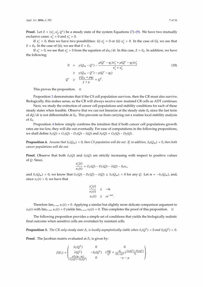
Proposition 5. The CR only steady state E1 is locally asymptotically stable when S1 (Q1) < 0 and S2 (Q

1) > 0.

Proof. The Jacobian matrix evaluated at E1 is given by:

J (E1) =*...,

S1 (Q1) 0 0

λ(Q1) −S2 (Q1) (

µq2Q2 +

d2(R2+Q )2

)G2 (Q1 )−D2 (Q1 )δ2

µδ2 (q1−q2 )

G2 (Q1 )−D2 (Q1 )0 −γ − µ

+///-

.

Appl. Sci. 2016, 6, 352 8 of 16

The eigenvalues are the diagonal elements. We see that when G1 (Q1) −D1 (Q

1) − λ1 (Q1) < 0 and

G2 (Q1) −D2 (Q

1) > 0, all diagonal elements are negative. Hence, E1 is locally asymptotically stable. �

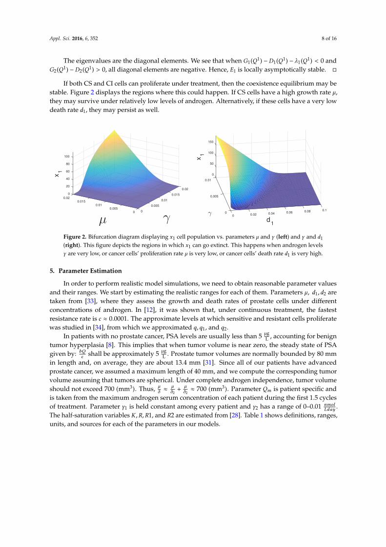
If both CS and CI cells can proliferate under treatment, then the coexistence equilibrium may bestable. Figure 2 displays the regions where this could happen. If CS cells have a high growth rate µ,they may survive under relatively low levels of androgen. Alternatively, if these cells have a very lowdeath rate d1, they may persist as well.

0.02

0.015

γ

0.01

0.005

000.005

µ

0.010.015

0.02

0

100

80

60

40

20

x1

0.10.080.060.04

d1

0.0200

0.005

150

0

50

100

0.01

γ

x1

Figure 2. Bifurcation diagram displaying x1 cell population vs. parameters µ and γ (left) and γ and d1(right). This figure depicts the regions in which x1 can go extinct. This happens when androgen levelsγ are very low, or cancer cells’ proliferation rate µ is very low, or cancer cells’ death rate d1 is very high.

5. Parameter Estimation

In order to perform realistic model simulations, we need to obtain reasonable parameter valuesand their ranges. We start by estimating the realistic ranges for each of them. Parameters µ, d1,d2 aretaken from [33], where they assess the growth and death rates of prostate cells under differentconcentrations of androgen. In [12], it was shown that, under continuous treatment, the fastestresistance rate is c ≈ 0.0001. The approximate levels at which sensitive and resistant cells proliferatewas studied in [34], from which we approximated q,q1, and q2.

In patients with no prostate cancer, PSA levels are usually less than 5 µgL , accounting for benign

tumor hyperplasia [8]. This implies that when tumor volume is near zero, the steady state of PSAgiven by: bQ

ϵ shall be approximately 5 µgL . Prostate tumor volumes are normally bounded by 80 mm

in length and, on average, they are about 13.4 mm [31]. Since all of our patients have advancedprostate cancer, we assumed a maximum length of 40 mm, and we compute the corresponding tumorvolume assuming that tumors are spherical. Under complete androgen independence, tumor volumeshould not exceed 700 (mm3). Thus, µ

δ ≈µδ2+

µδ2≈ 700 (mm3). Parameter Qm is patient specific and

is taken from the maximum androgen serum concentration of each patient during the first 1.5 cyclesof treatment. Parameter γ1 is held constant among every patient and γ2 has a range of 0–0.01 nmol

Lday .The half-saturation variables K ,R,R1, and R2 are estimated from [28]. Table 1 shows definitions, ranges,units, and sources for each of the parameters in our models.

Appl. Sci. 2016, 6, 352 9 of 16

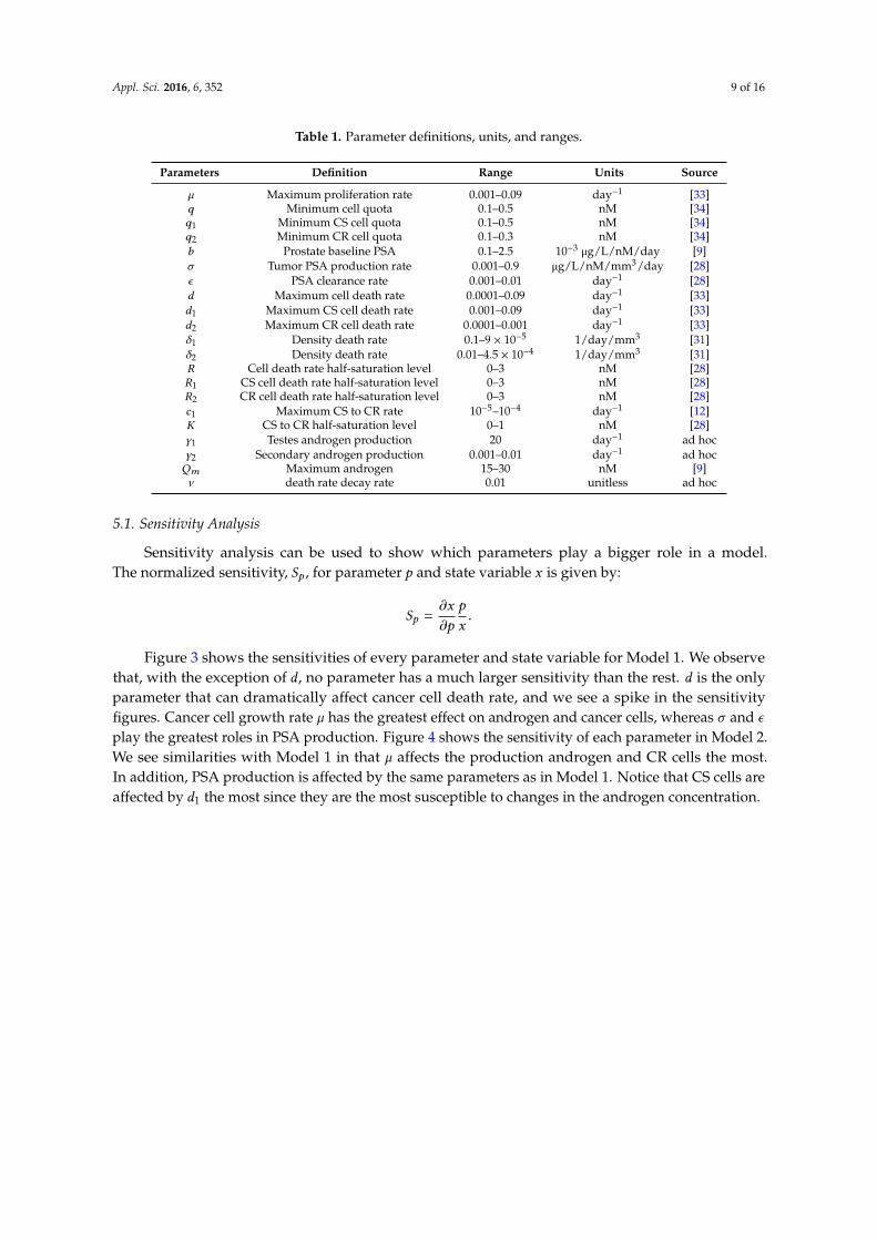
Table 1. Parameter definitions, units, and ranges.

Parameters Definition Range Units Source

µ Maximum proliferation rate 0.001–0.09 day−1 [33]q Minimum cell quota 0.1–0.5 nM [34]q1 Minimum CS cell quota 0.1–0.5 nM [34]q2 Minimum CR cell quota 0.1–0.3 nM [34]b Prostate baseline PSA 0.1–2.5 10−3 µg/L/nM/day [9]σ Tumor PSA production rate 0.001–0.9 µg/L/nM/mm3/day [28]ϵ PSA clearance rate 0.001–0.01 day−1 [28]d Maximum cell death rate 0.0001–0.09 day−1 [33]d1 Maximum CS cell death rate 0.001–0.09 day−1 [33]d2 Maximum CR cell death rate 0.0001–0.001 day−1 [33]δ1 Density death rate 0.1–9 × 10−5 1/day/mm3 [31]δ2 Density death rate 0.01–4.5 × 10−4 1/day/mm3 [31]R Cell death rate half-saturation level 0–3 nM [28]R1 CS cell death rate half-saturation level 0–3 nM [28]R2 CR cell death rate half-saturation level 0–3 nM [28]c1 Maximum CS to CR rate 10−5–10−4 day−1 [12]K CS to CR half-saturation level 0–1 nM [28]γ1 Testes androgen production 20 day−1 ad hocγ2 Secondary androgen production 0.001–0.01 day−1 ad hocQm Maximum androgen 15–30 nM [9]ν death rate decay rate 0.01 unitless ad hoc

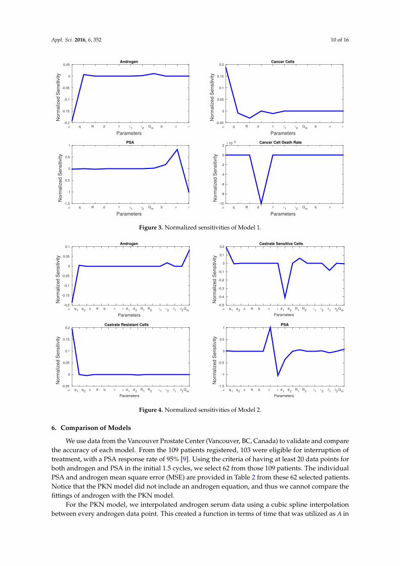
5.1. Sensitivity Analysis

Sensitivity analysis can be used to show which parameters play a bigger role in a model.The normalized sensitivity, Sp , for parameter p and state variable x is given by:

Sp =∂x

∂p

p

x.

Figure 3 shows the sensitivities of every parameter and state variable for Model 1. We observethat, with the exception of d, no parameter has a much larger sensitivity than the rest. d is the onlyparameter that can dramatically affect cancer cell death rate, and we see a spike in the sensitivityfigures. Cancer cell growth rate µ has the greatest effect on androgen and cancer cells, whereas σ and ϵ

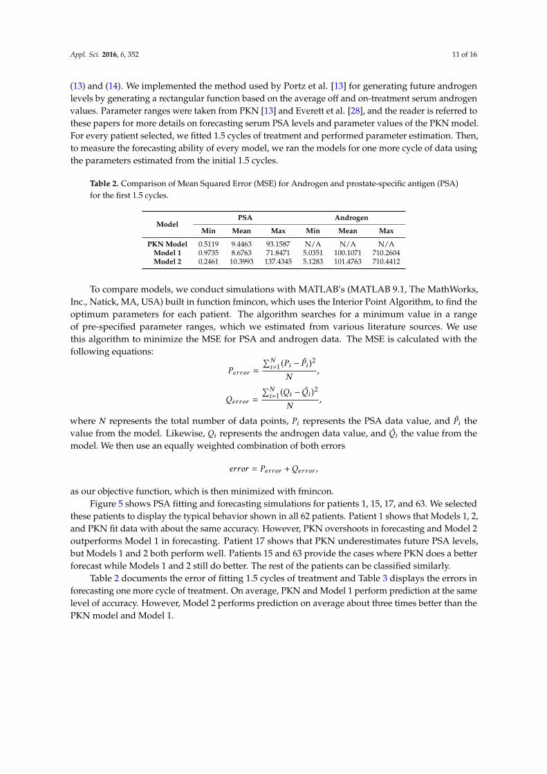
play the greatest roles in PSA production. Figure 4 shows the sensitivity of each parameter in Model 2.We see similarities with Model 1 in that µ affects the production androgen and CR cells the most.In addition, PSA production is affected by the same parameters as in Model 1. Notice that CS cells areaffected by d1 the most since they are the most susceptible to changes in the androgen concentration.

Appl. Sci. 2016, 6, 352 10 of 16

Parameters

µ q R d δ γ1

γ2

Qm

b σ ǫ

No

rma

lize

d S

en

sitiv

ity

-0.2

-0.15

-0.1

-0.05

0

0.05Androgen

Parameters

µ q R d δ γ1

γ2

Qm

b σ ǫ

No

rma

lize

d S

en

sitiv

ity

-0.05

0

0.05

0.1

0.15

0.2Cancer Cells

Parameters

µ q R d δ γ1

γ2

Qm

b σ ǫ

No

rma

lize

d S

en

sitiv

ity

-1.5

-1

-0.5

0

0.5

1PSA

Parameters

µ q R d δ γ1

γ2

Qm

b σ ǫ

No

rma

lize

d S

en

sitiv

ity

×10 -3

-10

-8

-6

-4

-2

0

2Cancer Cell Death Rate

Figure 3. Normalized sensitivities of Model 1.

Parameters

µ q1 q

2 c K b σ ǫ d

1 d

2 R

1 R

2 γ

1γ

2δ1

δ2

Qm

No

rma

lize

d S

en

sitiv

ity

-0.2

-0.15

-0.1

-0.05

0

0.05

0.1Androgen

Parameters

µ q1 q

2 c K b σ ǫ d

1 d

2 R

1 R

2 γ

1γ

2δ1

δ2

Qm

No

rma

lize

d S

en

sitiv

ity

-0.5

-0.4

-0.3

-0.2

-0.1

0

0.1

0.2Castrate Sensitive Cells

Parameters

µ q1 q

2 c K b σ ǫ d

1 d

2 R

1 R

2 γ

1γ

2δ1

δ2

Qm

No

rma

lize

d S

en

sitiv

ity

-0.05

0

0.05

0.1

0.15

0.2Castrate Resistant Cells

Parameters

µ q1 q

2 c K b σ ǫ d

1 d

2 R

1 R

2 γ

1γ

2δ1

δ2

Qm

No

rma

lize

d S

en

sitiv

ity

-1.5

-1

-0.5

0

0.5

1PSA

Figure 4. Normalized sensitivities of Model 2.

6. Comparison of Models

We use data from the Vancouver Prostate Center (Vancouver, BC, Canada) to validate and comparethe accuracy of each model. From the 109 patients registered, 103 were eligible for interruption oftreatment, with a PSA response rate of 95% [9]. Using the criteria of having at least 20 data points forboth androgen and PSA in the initial 1.5 cycles, we select 62 from those 109 patients. The individualPSA and androgen mean square error (MSE) are provided in Table 2 from these 62 selected patients.Notice that the PKN model did not include an androgen equation, and thus we cannot compare thefittings of androgen with the PKN model.

For the PKN model, we interpolated androgen serum data using a cubic spline interpolationbetween every androgen data point. This created a function in terms of time that was utilized as A in

Appl. Sci. 2016, 6, 352 11 of 16

(13) and (14). We implemented the method used by Portz et al. [13] for generating future androgenlevels by generating a rectangular function based on the average off and on-treatment serum androgenvalues. Parameter ranges were taken from PKN [13] and Everett et al. [28], and the reader is referred tothese papers for more details on forecasting serum PSA levels and parameter values of the PKN model.For every patient selected, we fitted 1.5 cycles of treatment and performed parameter estimation. Then,to measure the forecasting ability of every model, we ran the models for one more cycle of data usingthe parameters estimated from the initial 1.5 cycles.

Table 2. Comparison of Mean Squared Error (MSE) for Androgen and prostate-specific antigen (PSA)for the first 1.5 cycles.

ModelPSA Androgen

Min Mean Max Min Mean Max

PKN Model 0.5119 9.4463 93.1587 N/A N/A N/AModel 1 0.9735 8.6763 71.8471 5.0351 100.1071 710.2604Model 2 0.2461 10.3993 137.4345 5.1283 101.4763 710.4412

To compare models, we conduct simulations with MATLAB’s (MATLAB 9.1, The MathWorks,Inc., Natick, MA, USA) built in function fmincon, which uses the Interior Point Algorithm, to find theoptimum parameters for each patient. The algorithm searches for a minimum value in a rangeof pre-specified parameter ranges, which we estimated from various literature sources. We usethis algorithm to minimize the MSE for PSA and androgen data. The MSE is calculated with thefollowing equations:

Perror =

∑Ni=1 (Pi − P̂i )

2

N,

Qerror =

∑Ni=1 (Qi − Q̂i )

2

N,

where N represents the total number of data points, Pi represents the PSA data value, and P̂i thevalue from the model. Likewise, Qi represents the androgen data value, and Q̂i the value from themodel. We then use an equally weighted combination of both errors

error = Perror +Qerror ,

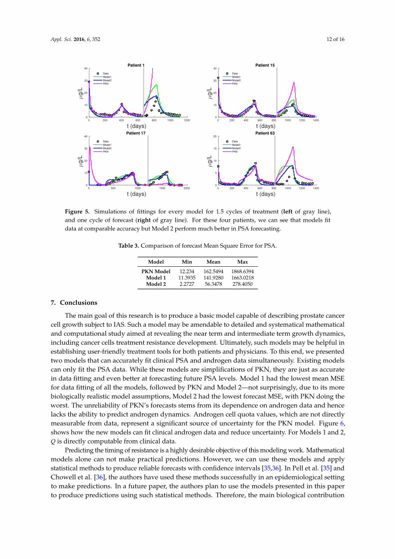
as our objective function, which is then minimized with fmincon.Figure 5 shows PSA fitting and forecasting simulations for patients 1, 15, 17, and 63. We selected

these patients to display the typical behavior shown in all 62 patients. Patient 1 shows that Models 1, 2,and PKN fit data with about the same accuracy. However, PKN overshoots in forecasting and Model 2outperforms Model 1 in forecasting. Patient 17 shows that PKN underestimates future PSA levels,but Models 1 and 2 both perform well. Patients 15 and 63 provide the cases where PKN does a betterforecast while Models 1 and 2 still do better. The rest of the patients can be classified similarly.

Table 2 documents the error of fitting 1.5 cycles of treatment and Table 3 displays the errors inforecasting one more cycle of treatment. On average, PKN and Model 1 perform prediction at the samelevel of accuracy. However, Model 2 performs prediction on average about three times better than thePKN model and Model 1.

Appl. Sci. 2016, 6, 352 12 of 16

t (days)0 200 400 600 800 1000 1200

µg

/L

0

10

20

30

40Patient 1

Data

Model1

Model2

PKN

t (days)0 200 400 600 800 1000 1200 1400

µg

/L

0

10

20

30

40Patient 15

Data

Model1

Model2

PKN

t (days)0 500 1000 1500 2000

µg

/L

0

10

20

30

40Patient 17

Data

Model1

Model2

PKN

t (days)0 200 400 600 800 1000 1200 1400

µg

/L

0

5

10

15

20Patient 63

Data

Model1

Model2

PKN

Figure 5. Simulations of fittings for every model for 1.5 cycles of treatment (left of gray line),and one cycle of forecast (right of gray line). For these four patients, we can see that models fitdata at comparable accuracy but Model 2 perform much better in PSA forecasting.

Table 3. Comparison of forecast Mean Square Error for PSA.

Model Min Mean Max

PKN Model 12.234 162.5494 1868.6394Model 1 11.3935 141.9280 1663.0218Model 2 2.2727 56.3478 278.4050

7. Conclusions

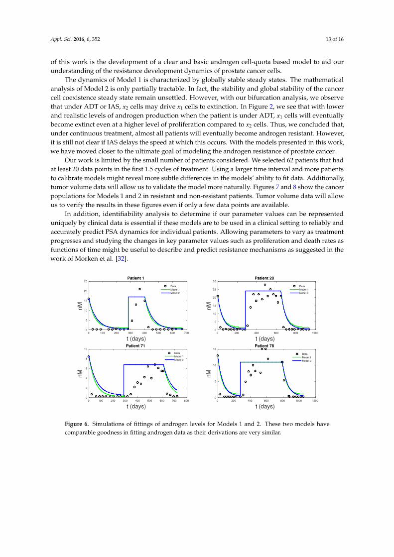
The main goal of this research is to produce a basic model capable of describing prostate cancercell growth subject to IAS. Such a model may be amendable to detailed and systematical mathematicaland computational study aimed at revealing the near term and intermediate term growth dynamics,including cancer cells treatment resistance development. Ultimately, such models may be helpful inestablishing user-friendly treatment tools for both patients and physicians. To this end, we presentedtwo models that can accurately fit clinical PSA and androgen data simultaneously. Existing modelscan only fit the PSA data. While these models are simplifications of PKN, they are just as accuratein data fitting and even better at forecasting future PSA levels. Model 1 had the lowest mean MSEfor data fitting of all the models, followed by PKN and Model 2—not surprisingly, due to its morebiologically realistic model assumptions, Model 2 had the lowest forecast MSE, with PKN doing theworst. The unreliability of PKN’s forecasts stems from its dependence on androgen data and hencelacks the ability to predict androgen dynamics. Androgen cell quota values, which are not directlymeasurable from data, represent a significant source of uncertainty for the PKN model. Figure 6,shows how the new models can fit clinical androgen data and reduce uncertainty. For Models 1 and 2,Q is directly computable from clinical data.

Predicting the timing of resistance is a highly desirable objective of this modeling work. Mathematicalmodels alone can not make practical predictions. However, we can use these models and applystatistical methods to produce reliable forecasts with confidence intervals [35,36]. In Pell et al. [35] andChowell et al. [36], the authors have used these methods successfully in an epidemiological settingto make predictions. In a future paper, the authors plan to use the models presented in this paperto produce predictions using such statistical methods. Therefore, the main biological contribution

Appl. Sci. 2016, 6, 352 13 of 16

of this work is the development of a clear and basic androgen cell-quota based model to aid ourunderstanding of the resistance development dynamics of prostate cancer cells.

The dynamics of Model 1 is characterized by globally stable steady states. The mathematicalanalysis of Model 2 is only partially tractable. In fact, the stability and global stability of the cancercell coexistence steady state remain unsettled. However, with our bifurcation analysis, we observethat under ADT or IAS, x2 cells may drive x1 cells to extinction. In Figure 2, we see that with lowerand realistic levels of androgen production when the patient is under ADT, x1 cells will eventuallybecome extinct even at a higher level of proliferation compared to x2 cells. Thus, we concluded that,under continuous treatment, almost all patients will eventually become androgen resistant. However,it is still not clear if IAS delays the speed at which this occurs. With the models presented in this work,we have moved closer to the ultimate goal of modeling the androgen resistance of prostate cancer.

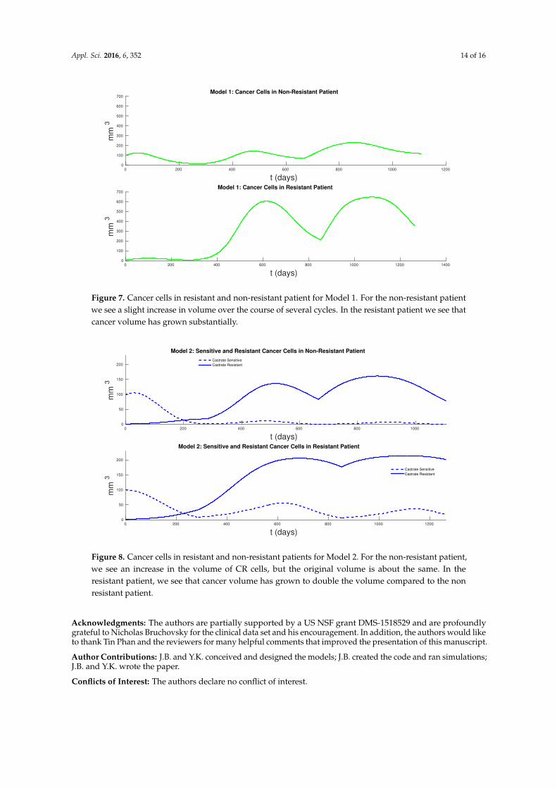
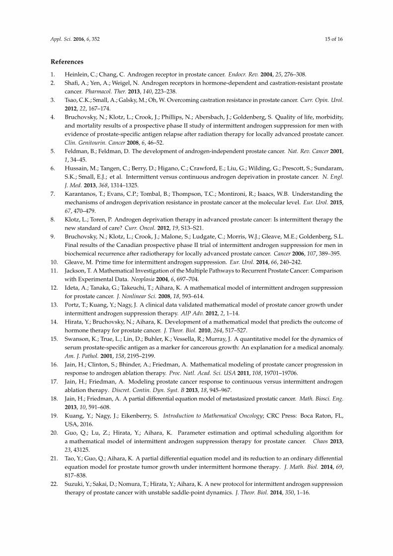
Our work is limited by the small number of patients considered. We selected 62 patients that hadat least 20 data points in the first 1.5 cycles of treatment. Using a larger time interval and more patientsto calibrate models might reveal more subtle differences in the models’ ability to fit data. Additionally,tumor volume data will allow us to validate the model more naturally. Figures 7 and 8 show the cancerpopulations for Models 1 and 2 in resistant and non-resistant patients. Tumor volume data will allowus to verify the results in these figures even if only a few data points are available.

In addition, identifiability analysis to determine if our parameter values can be representeduniquely by clinical data is essential if these models are to be used in a clinical setting to reliably andaccurately predict PSA dynamics for individual patients. Allowing parameters to vary as treatmentprogresses and studying the changes in key parameter values such as proliferation and death rates asfunctions of time might be useful to describe and predict resistance mechanisms as suggested in thework of Morken et al. [32].

t (days)0 100 200 300 400 500 600 700

nM

0

5

10

15

20

25Patient 1

Data

Model 1

Model 2

t (days)0 200 400 600 800 1000

nM

0

5

10

15

20

25

30Patient 28

Data

Model 1

Model 2

t (days)0 100 200 300 400 500 600 700 800

nM

0

2

4

6

8

10Patient 71

Data

Model 1

Model 2

t (days)0 200 400 600 800 1000 1200

nM

0

5

10

15Patient 78

Data

Model 1

Model 2

Figure 6. Simulations of fittings of androgen levels for Models 1 and 2. These two models havecomparable goodness in fitting androgen data as their derivations are very similar.

Appl. Sci. 2016, 6, 352 14 of 16

t (days)0 200 400 600 800 1000 1200

mm

3

0

100

200

300

400

500

600

700Model 1: Cancer Cells in Non-Resistant Patient

t (days)0 200 400 600 800 1000 1200 1400

mm

3

0

100

200

300

400

500

600

700Model 1: Cancer Cells in Resistant Patient

Figure 7. Cancer cells in resistant and non-resistant patient for Model 1. For the non-resistant patientwe see a slight increase in volume over the course of several cycles. In the resistant patient we see thatcancer volume has grown substantially.

t (days)0 200 400 600 800 1000

mm

3

0

50

100

150

200

Model 2: Sensitive and Resistant Cancer Cells in Non-Resistant Patient

Castrate Sensitive

Castrate Resistant

t (days)0 200 400 600 800 1000 1200

mm

3

0

50

100

150

200

Model 2: Sensitive and Resistant Cancer Cells in Resistant Patient

Castrate Sensitive

Castrate Resistant

Figure 8. Cancer cells in resistant and non-resistant patients for Model 2. For the non-resistant patient,we see an increase in the volume of CR cells, but the original volume is about the same. In theresistant patient, we see that cancer volume has grown to double the volume compared to the nonresistant patient.

Acknowledgments: The authors are partially supported by a US NSF grant DMS-1518529 and are profoundlygrateful to Nicholas Bruchovsky for the clinical data set and his encouragement. In addition, the authors would liketo thank Tin Phan and the reviewers for many helpful comments that improved the presentation of this manuscript.

Author Contributions: J.B. and Y.K. conceived and designed the models; J.B. created the code and ran simulations;J.B. and Y.K. wrote the paper.

Conflicts of Interest: The authors declare no conflict of interest.

Appl. Sci. 2016, 6, 352 15 of 16

References

1. Heinlein, C.; Chang, C. Androgen receptor in prostate cancer. Endocr. Rev. 2004, 25, 276–308.2. Shafi, A.; Yen, A.; Weigel, N. Androgen receptors in hormone-dependent and castration-resistant prostate

cancer. Pharmacol. Ther. 2013, 140, 223–238.3. Tsao, C.K.; Small, A.; Galsky, M.; Oh, W. Overcoming castration resistance in prostate cancer. Curr. Opin. Urol.

2012, 22, 167–174.4. Bruchovsky, N.; Klotz, L.; Crook, J.; Phillips, N.; Abersbach, J.; Goldenberg, S. Quality of life, morbidity,

and mortality results of a prospective phase II study of intermittent androgen suppression for men withevidence of prostate-specific antigen relapse after radiation therapy for locally advanced prostate cancer.Clin. Genitourin. Cancer 2008, 6, 46–52.

5. Feldman, B.; Feldman, D. The development of androgen-independent prostate cancer. Nat. Rev. Cancer 2001,1, 34–45.

6. Hussain, M.; Tangen, C.; Berry, D.; Higano, C.; Crawford, E.; Liu, G.; Wilding, G.; Prescott, S.; Sundaram,S.K.; Small, E.J.; et al. Intermittent versus continuous androgen deprivation in prostate cancer. N. Engl.J. Med. 2013, 368, 1314–1325.

7. Karantanos, T.; Evans, C.P.; Tombal, B.; Thompson, T.C.; Montironi, R.; Isaacs, W.B. Understanding themechanisms of androgen deprivation resistance in prostate cancer at the molecular level. Eur. Urol. 2015,67, 470–479.

8. Klotz, L.; Toren, P. Androgen deprivation therapy in advanced prostate cancer: Is intermittent therapy thenew standard of care? Curr. Oncol. 2012, 19, S13–S21.

9. Bruchovsky, N.; Klotz, L.; Crook, J.; Malone, S.; Ludgate, C.; Morris, W.J.; Gleave, M.E.; Goldenberg, S.L.Final results of the Canadian prospective phase II trial of intermittent androgen suppression for men inbiochemical recurrence after radiotherapy for locally advanced prostate cancer. Cancer 2006, 107, 389–395.

10. Gleave, M. Prime time for intermittent androgen suppression. Eur. Urol. 2014, 66, 240–242.11. Jackson, T. A Mathematical Investigation of the Multiple Pathways to Recurrent Prostate Cancer: Comparison

with Experimental Data. Neoplasia 2004, 6, 697–704.12. Ideta, A.; Tanaka, G.; Takeuchi, T.; Aihara, K. A mathematical model of intermittent androgen suppression

for prostate cancer. J. Nonlinear Sci. 2008, 18, 593–614.13. Portz, T.; Kuang, Y.; Nagy, J. A clinical data validated mathematical model of prostate cancer growth under

intermittent androgen suppression therapy. AIP Adv. 2012, 2, 1–14.14. Hirata, Y.; Bruchovsky, N.; Aihara, K. Development of a mathematical model that predicts the outcome of

hormone therapy for prostate cancer. J. Theor. Biol. 2010, 264, 517–527.15. Swanson, K.; True, L.; Lin, D.; Buhler, K.; Vessella, R.; Murray, J. A quantitative model for the dynamics of

serum prostate-specific antigen as a marker for cancerous growth: An explanation for a medical anomaly.Am. J. Pathol. 2001, 158, 2195–2199.

16. Jain, H.; Clinton, S.; Bhinder, A.; Friedman, A. Mathematical modeling of prostate cancer progression inresponse to androgen ablation therapy. Proc. Natl. Acad. Sci. USA 2011, 108, 19701–19706.

17. Jain, H.; Friedman, A. Modeling prostate cancer response to continuous versus intermittent androgenablation therapy. Discret. Contin. Dyn. Syst. B 2013, 18, 945–967.

18. Jain, H.; Friedman, A. A partial differential equation model of metastasized prostatic cancer. Math. Biosci. Eng.2013, 10, 591–608.

19. Kuang, Y.; Nagy, J.; Eikenberry, S. Introduction to Mathematical Oncology; CRC Press: Boca Raton, FL,USA, 2016.

20. Guo, Q.; Lu, Z.; Hirata, Y.; Aihara, K. Parameter estimation and optimal scheduling algorithm fora mathematical model of intermittent androgen suppression therapy for prostate cancer. Chaos 2013,23, 43125.

21. Tao, Y.; Guo, Q.; Aihara, K. A partial differential equation model and its reduction to an ordinary differentialequation model for prostate tumor growth under intermittent hormone therapy. J. Math. Biol. 2014, 69,817–838.

22. Suzuki, Y.; Sakai, D.; Nomura, T.; Hirata, Y.; Aihara, K. A new protocol for intermittent androgen suppressiontherapy of prostate cancer with unstable saddle-point dynamics. J. Theor. Biol. 2014, 350, 1–16.

Appl. Sci. 2016, 6, 352 16 of 16

23. Hirata, Y.; Akakura, K.; Higano, C.; Bruchovsky, N.; Aihara, K. Quantitative mathematical modeling of PSAdynamics of prostate cancer patients treated with intermittent androgen suppression. J. Mol. Cell Biol. 2012,4, 127–132.

24. Hirata, Y.; Tanaka, G.; Bruchovsky, N.; Aihara, K. Mathematically modelling and controlling prostate cancerunder intermittent hormone therapy. Asian J. Androl. 2012, 14, 270–277.

25. Hirata, Y.; Azuma, S.; Aihara, K. Model predictive control for optimally scheduling intermittent androgensuppression of prostate cancer. Methods 2014, 67, 278–281.

26. Jackson, T. A mathematical model of prostate tumor growth and androgen-independent relapse. Discret. Contin.Dyn. Syst. B 2004, 4, 187–202.

27. Droop, M. Some thoughts on nutrient limitation in algae1. J. Phycol. 1973, 9, 264–272.28. Everett, R.; Packer, A.; Kuang, Y. Can Mathematical Models Predict the Outcomes of Prostate Cancer Patients

Undergoing Intermittent Androgen Deprivation Therapy? Biophys. Rev. Lett. 2014, 9, 173–191.29. Roy, A.; Chatterjee, B. Androgen action. Crit. Rev. Eukaryot. Gene Expr. 1995, 5, 157–176.30. Bruchovsky, N. Clinical Research. 2006. Available online: http://www.nicholasbruchovsky.com/clinicalResearch.

html (accessed on 11 November 2016).31. Vollmer, R. Tumor Length in Prostate Cancer. Am. J. Clin. Pathol. 2008, 130, 77–82.32. Morken, J.; Packer, A.; Everett, R.; Nagy, J.; Kuang, Y. Mechanisms of resistance to intermittent androgen

deprivation in patients with prostate cancer identified by a novel computational method. Cancer Res. 2014,74, 3673–3683.

33. Berges, R.R.; Vukanovic, J.; Epstein, J.I.; CarMichel, M.; Cisek, L.; Johnson, D.E.; Veltri, R.W.; Walsh, P.C.; Isaacs, J.T.Implication of cell kinetic changes during the progression of human prostatic cancer. Clin. Cancer Res. 1995,1, 473–480.

34. Nishiyama, T. Serum testosterone levels after medical or surgical androgen deprivation: A comprehensivereview of the literature. Urol. Oncol. 2013, 32, 38.e17–38.e28.

35. Pell, B.; Baez, J.; Phan, T.; Gao, D.; C, G.; Kuang, Y. Patch Models of EVD Transmission Dynamics; Springer:Cham, Switzerland, 2016.

36. Chowell, G.; Simonsen, L.; Kuang, Y.; Sciences, S. Is West Africa Approaching a Catastrophic Phaseor is the 2014 Ebola Epidemic Slowing Down? Different Models Yield Different Answers for Liberia.PLOS Curr. Outbreaks 2014, doi:10.1371/currents.outbreaks.b4690859d91684da963dc40e00f3da81.

c© 2016 by the authors; licensee MDPI, Basel, Switzerland. This article is an open accessarticle distributed under the terms and conditions of the Creative Commons Attribution(CC-BY) license (http://creativecommons.org/licenses/by/4.0/).