MITNE-1 92

MATHEMATICAL MODELS FORPREDICTING THE THERMAL PERFORMANCE

OF CLOSED-CYCLE WASTE HEATDISSIPATION SYSTEMS

by

ERIC C. GUYER

andMICHAEL W. GOLAY

October, 1976

DEPARTMENT OF NUCLEAR ENGINEERINGMASSACHUSETTS INSTITUTE OF TECHNOLOGY

77 Massachusetts AvenueCambridge, Massachusetts 02139

Massachusetts Institute of TechnologyDepartment of Nuclear Engineering

Cambridge, Massachusetts

Mathematical Models for Predicting the Thermal

Performance of Closed-Cycle Waste Heat

Dissipation Systems

by

Eric C. Guyer and Michael W. Golay

:1

ABSTRACT

The literature concerning the mathematical modelling

of the thermal performance of closed-cycle waste heat dissi-

pation systems for the steam-electric plant is critically

examined. Models suitable for survey analysis of waste

heat systems are recommended. The specific models discussed

are those for a mechanical draft evaporative cooling tower,

a natural draft evaporative cooling tower, a spray canal,

a plug-flow cooling pond, and a mechanical or natural draft

dry cooling tower. FORTRAN computer programs of these models

are included to facilitate their application.

2

TABLE OF CONTENTS

ABSTRACT

TABLE OF CONTENTS

LIST OF FIGURES

LIST OF TABLES

CHAPTER 1. INTRODUCTION

CHAPTER 2. MATHEMATICAL MODELS FOR PREDICTING THETHERMAL PERFORMANCE OF CLOSED-CYCLE WASTEHEAT DISSIPATION SYSTEMS

2.1 Introduction

2.2 .Mechanical Draft Evaporative Cooling Towers

2.2.1 Literature Review

2.2.2 Selection of Model

2.2.3 Application of Model

2.3 Spray Systems

2.3.1 Literature Review

2.3.2 Selection of Model

2.4 Natural Draft Evaporative Cooling Towers

2.4.1 Literature Review

2.4.2 Selection of Model

2.5 Cooling Ponds

2.5.1 Literature Review

2.5.2 Selection of Model

2.6 Dry Cooling Towers

APPENDIX A. COMPUTER PROGRAMS FOR WASTE HEAT REJECTIONSYSTEM THERMAL PERFORMANCE CALCULATIONS

Page

I

2

3

4

5

6

6

9

9

13

18

21

21

23

26

26

28

33

33

35

37

45

3

LIST OF FIGURES

2.1 Illustration of Tower-fill Finite-Difference Calcu-lation 15

2.2 Calculational Algorithm for Prediction the Perfor-mance of Mechanical-Draft Cross-Flow EvaporativeCooling Tower 17

2.3 Comparison of Reported and Predicted MechanicalDraft Cooling Tower Performance 20

2.4 Computational Algorithm for Spray Canal ThermalPerformance Model 24

2.5 Calculational Algorithm for Natural-Draft EvaporativeCooling Tower Performance Model 29

2.6 Comparison of Reported and Predicted Natural-DraftCooling Tower Performance 32

2.7 Cooling Pond Model Computational Algorithm 38

2.8 Dry Cooling Tower Schematic Drawing 40

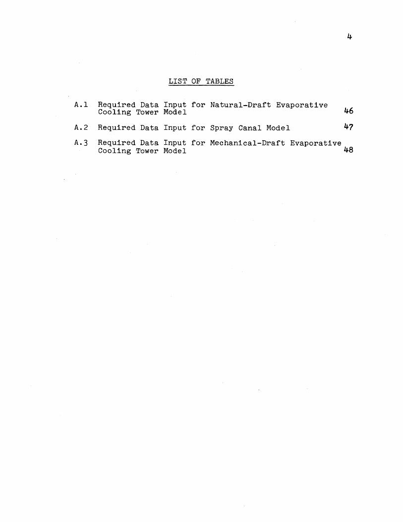
LIST OF TABLES

A.1 Required Data Input for Natural-Draft EvaporativeCooling Tower Model 46

A.2 Required Data Input for Spray Canal Model 47

A.3 Required Data Input for Mechanical-Draft EvaporativeCooling Tower Model 48

5

CHAPTER 1

INTRODUCTION

A study of mixed-mode waste heat dissipation systems

for steam-electric plants has been performed in the Nuclear

Engineering Department [28]. Mixed-mode waste heat dissipa-

tion systems are defined as those waste heat dissipation

systems composed of combination of two or more different

heat rejection devices or those waste heat dissipation sys-

tems operated with variable cycles. This report summarizes

the mathematical thermal-performance models of the various

component waste heat systems which were developed in the

completion of this study. The thermal-performance models

presented in this report are those for a mechanical-draft

evaporative cooling tower, a natural-draft evaporative

cooling tower, a spray canal, a plug-flow cooling pond, and

a natural or mechanical draft dry cooling tower. These

models are recdmmended for survey-type analyses of waste

heat rejection systems.

Chapter 2 includes a review of literature pertaining to

the mathematical modeling of each of these heat rejection

devices and a discussion of the assumptions inherent to the

recommended models. Appendix A contains FORTRAN program list-

ings of the recommended models and a description of the re-

quired input data for each of the models.

6

CHAPTER 2

MATHEMATICAL MODELS FOR PREDICTING THE THERMAL

PERFORMANCE OF CLOSED-CYCLE WASTE HEAT

DISSIPATION SYSTEMS

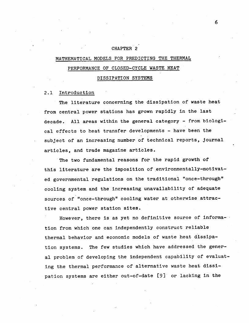
2.1 Introduction

The literature concerning the dissipation of waste heat

from central power stations has grown rapidly in the last

decade. All areas within the general category - from biologi-

cal effects to heat transfer developments - have been the

subject of an increasing number of technical reports, journal

articles, and trade magazine articles.

The two fundamental reasons for the rapid growth of

this literature are the imposition of.environmentally-motivat-

ed governmental regulations on the traditional "once-through"

cooling system and the increasing unavailability of adequate

sources of "once-through" cooling water at otherwise attrac-

tive central power station sites.

However, there is as yet no definitive source of informa-

tion from which one can independently construct reliable

thermal behavior and economic models of waste heat dissipa-

tion systems. The few studies which have addressed the gener-

al problem of developing the independent capability of evaluat-

ing the thermal performance of alternative waste heat.dissi-

pation systems are either out-of-date [9] or lacking in the

?

details 13] [10] and thus c'an not be directly applied to

the present task. Thus, considerable effort was required

to review the available information and compile it into a

useful tool for evaluating the costs/benefits of various

alternative waste heat dissipation schemes.

The available literature concerning the mathematical

modeling of the economics and thermal behavior of waste

heat systems has been authored primarily by 1) the vendors

of waste heat dissipation equipment, 2) the electric utility

incistry, and 3) various research institutes and universi-

ties. In view of the present task of developing accurate

mathematical models of conventional waste heat rejection

devices some general comments can be made about the litera-

ture with regard to its authorship.

Although there has been a tremendous increase in the

waste heat dissipation equipment vendor sector in both size

and diversity, the publications of these vendors are gener-

ally qualitative in nature. With a few notable exceptions,

the literature published does not deal quantitatively with

thermal behavior analysis, but, rather, describes qualita-

tively the particular vendors present capabilities and high-

lights the economic advantages of the particular vendors

devices. Little of this information is of value to those

interested in developing an independent analysis capability.

8

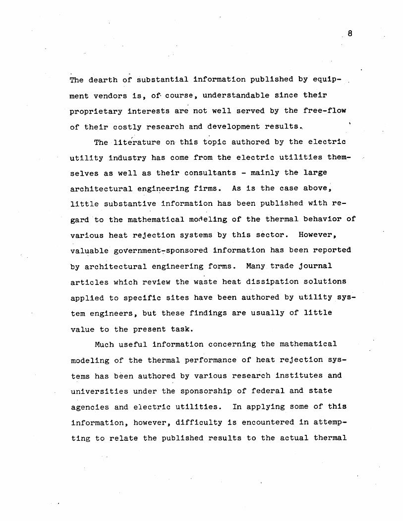
The dearth of substantial information published by equip-

ment vendors is, of- course, understandable since their

proprietary interests are not well served by the free-flow

of their costly research and development results..

The literature on this topic authored by the electric

utility industry has come from the electric utilities them-

selves as well as their consultants - mainly the large

architectural engineering firms. As is the case above,

little substantive information has been published with re-

gard to the mathematical modeling of the thermal behavior of

various heat rejection systems by this sector. However,

valuable government-sponsored information has been reported

by architectural engineering forms. Many trade journal

articles which review the waste heat dissipation solutions

applied to specific sites have been authored by utility sys-

tem engineers, but these findings are usually of little

value to the present task.

Much useful information concerning the mathematical

modeling of the thermal performance of heat rejection sys-

tems has been authored by various research institutes and

universities under the sponsorship of federal and state

agencies and electric utilities. In applying some of this

information, however, difficulty is encountered in attemp-

ting to relate the published results to the actual thermal

9

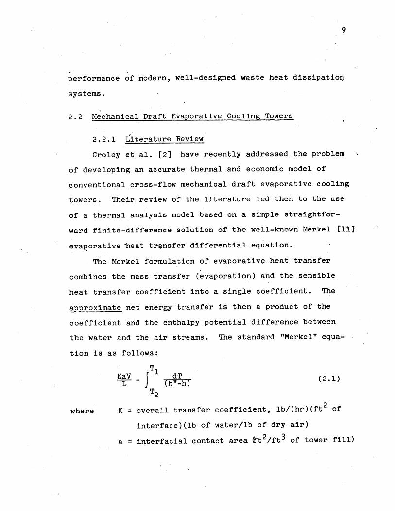
performance of modern, well-designed waste heat dissipation

systems.

2.2 Mechanical Draft Evaporative Cooling Towers

2,2.1 Literature Review

Croley et al. [2] have recently addressed the problem

of developing an accurate thermal and economic model of

conventional cross-flow mechanical draft evaporative cooling

towers. Their review of the literature led then to the use

of a thermal analysis model based on a simple straightfor-

ward finite-difference solution of the well-known Merkel [11]

evaporative 'heat transfer differential equation.

The Merkel formulation of evaporative heat transfer

combines the mass transfer (evaporation) and the sensible

heat transfer coefficient into a single coefficient. The

approximate net energy transfer is then a product of the

coefficient and the enthalpy potential difference between

the water and the air streams. The standard "Merkel" equa-

tion is as follows:

T1KaV dT (2.1)

L J (h"-h)T 2

where K = overall transfer coefficient, lb/(hr)(ft2 of

interface)(lb of water/lb of dry air)

a = interfacial contact area (ft2/ft3 of tower fill)

10

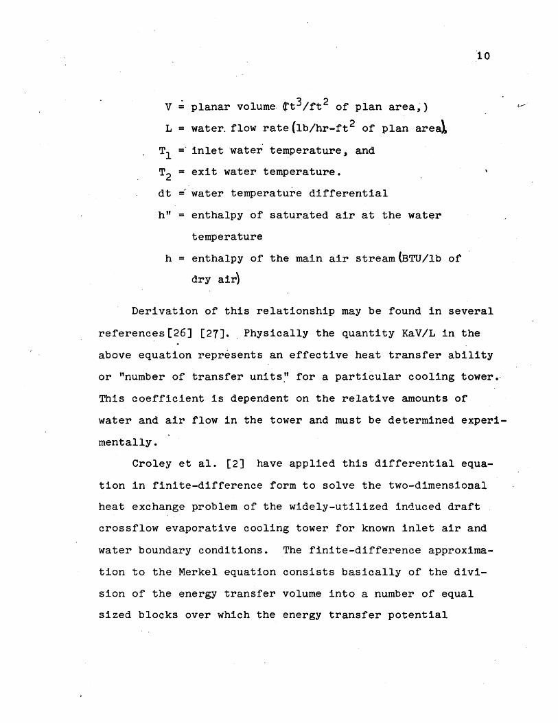
V = planar volume It 3/ft 2 of plan area,)

L = water. flow rate(lb/hr-ft2 of plan areal

T inlet water temperature, and

T2= exit water temperature.

dt water temperature differential

h"= enthalpy of saturated air at the water

temperature

h = enthalpy of the main air stream(BTU/lb of

dry air)

Derivation of this relationship may be found in several

references[26] [27]., Physically the quantity KaV/L in the

above equation represents an effective heat transfer ability

or "number of transfer units" for a particular cooling tower.

This coefficient is dependent on the relative amounts of

water and air flow in the tower and must be determined experi-

mentally.

Croley et al. [2] have applied this differential equa-

tion in finite-difference form to solve the two-dimensional

heat exchange problem of the widely-utilized induced draft

crossflow evaporative cooling tower for known inlet air and

water boundary conditions. The finite-difference approxima-

tion to the Merkel equation consists basically of the divi-

sion of the energy transfer volume into a number of equal

sized blocks over which the energy transfer potential

11

(enthalpy) is averaged.

The conclusions of Croley et al. concerning the utility.

of the .basic Merkel formulation for the predicting of the

energy transfer in a cooling tower has since been substanti-

ated by the recommendation of Hallet [12]. Hallet, repre-

senting a leading cooling tower vendor, has suggested that

the best approach (for a non-vendor) to the problem of

evaluating the thermal performance of wet cross-flow towers

is a finite-difference solution of the basic Merkel equation.

This author also points out that, although many improvements

in the theory of simultaneous heat and mass transfer at

water/air interfaces have been suggested, the basic Merkel

formulation is the only widely accepted and proven theory.

The analysis technique suggested by Hallet is essentially

identical to that of Croley et al. except that Hallet recom-

mends the inclusion of a temperature dependence in the expres-

sion for the tower fill energy transfer coefficient:

Ka = f(T1 ) (2.2)

where T is the tower inlet water temperature. It. is interes-

ting to note that no physical justification is given by

Hallet for this "temperature effect". Consideration of

recent works which address the errors inherent to the Merkel

equation suggest that this "temperature effect" fixup is

12

necessary because of errors- in the Merkel approximate formu-

lation for evaporative heat transfer.

The investigations of Nahavandi [13] and Yadigaroglu

[14] have been concerned with an evaluation of the errors in-

herent to Merkel equation. The results of Yadigaroglu are

based on a comparison of the predictions of the Merkel

theory and a more exact and complete theory which treats the

mass and sensible heat processes separately. This investi-

gator found that the effect of the various approximations of

the Merkel theory tends to be small since the different approxi-

mations of the Merkel theory result in partially cancelling

positive and- negative errors. The conclusion is that, given

the other errors associated with cooling tower performance

predictions (uniform air and water flow rates, for example)

and performance verifications (experimental uncertainties),

the added complexity of performing the more exact energy

transfer analysis is not justified. Nevertheless, it is of

interest to note that Yadigaroglu found that the net positive

error in predicting the cooling range increased with increas-

ing air inlet temperature and humidity. This error could be

corrected by arbitrarily decreasing the value of KaV/L by

the appropriate amount as the water inlet temperature increas-

ed. Indeed, this is the same, but unjustified, approach

recommended by Hallet. Examining the magnitude of the over-

i3

prediction resulting from the use of Merkel theory ( on the

order of 5%), it is found that the Merkel theory error is

consistent with the suggested "temperature effect" correc-

tion of KaV/L (about 5% per 10 OF rise in inlet water temp-

erature for inlet water temperatures in excess of 90 OF).

2.2.2 Selection of a Model

The mathematical model to be used in the prediction of

the thermal performance of mechanical draft evaporative

cooling towers is the finite-difference approximation of the

Merkel equation. The finite-difference approximation to the

Merkel equation can be stated as [2]

r I IKaV h i-h + h -h0

G(h0-hi) = N - 2

h and

h and

h = saturated air enthalpies at the inlet

and outlet of an incremental element,

h = saturated air enthalpies at the temp-

erature of the water entering and

leaving the incremental element,

G = air flow rate per incremental element,

N = square root of the number of incremen-

tal elements, and

KaV = transfer coefficient.

(2-3)

where

14

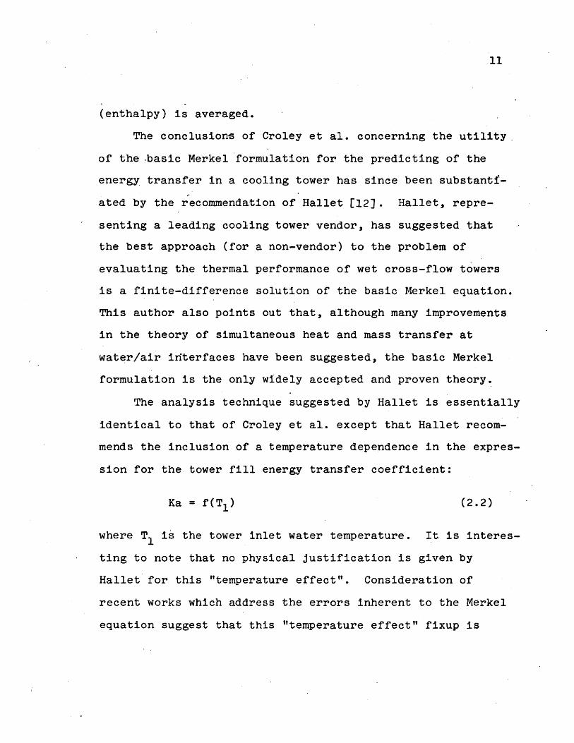
The application of this equation to the cross-flow prob-

lem of a conventional induced draft cross-flow cooling tower

is shown in Fig. 2.1.

In addition to the above equation, the energy balance

equation

G(h -h ) = c pL(t -t = L(h -h0) (2.4)

is needed to completely describe the temperature history of

the air and water as it passes through the tower fill. In

the above equation:

L = water loading per incremental element,

t and to inlet .and outlet water temperatures for an

incremental element, and

c = specific heat capacity of water.

Equations 2.3 and 2.4 form a set of coupled equations

with unknown variables h0 and h0 which must be solved for

iteratively. The algorithm for calculating the average out-.

let water temperature and average outlet air temperature is

given in Fig. 2.2. Note thta, for practical purposes, the

water and air flow rates are fixed by the tower design and

to a good approximation can be assumed to be uniform and

constant throughout the tower. Note, also, that the algorithm

is for calculating the performance of a given tower design.

If we wish to find the size of the tower needed to meet a

15Fig. 2.1

Illustration of Tower Fill Finite-Difference Calculatton

L

unit

Tower Fill

Structure

lenght

L, hl

4'Unit Cell

H= N

H=NEX

A~Y

1LG,hI

hK

H

ho

1-6

specific cooling requirement, a trial and error calculation

may be performed.

The saturated air enthalpy used as the driving poten-

tial in the Merkel equation depends on both the dry bulb

temperature and the humidity of the air. However, a good

approximation to the enthalpy which depends solely. on the

thermodynamic wet bulb temperature may be derived. From

Marks [15) we have the relationship,

E = 0.24Td + w(1062.0 + O.4 4Td) (2.5)

and

W* - (0.24 + 0.44W*)(Td - Twb)W = (2.6)

(1094 + 0.44Td - Twb)

where E = enthalpy of moist air,

Td = dry bulb temperature,

W = specific humidity,

Twb = wet bulb temperature, and

W* = specific humidity for saturation at Twb.

Substituting the latter into the former we have

E = 0.24Td + W*(1062 + .44Td) -

(0.24 +0.44W*)(Td-Twb)(l062+ 0.44Td) (2.7)(1094 + 0.k44Td-Twb)(

17

Fig.- 2.2

Calculational Algorithm for Predicting the Performanceof Mechanical Draft Cross-flow Evaporative

. Cooling Tower (MECDRAFT Program)

Determine inlet air and water enthalpies

Iteratively calculate h' and h0 for eachelement of the top row starting at the

air inlet side (equations 2.3 and 2.4 )

-4For the next lower row of elements iterativelycalculate ho and ho starting from the air in-

let side (equations 2.3 and 2.4) IDetermine if bottom of tower attained

I.

YES

Average outlet air and water temperatures foreach horizontal and vertical row respectively

End

NO

4

I

18

Now assuming that in the deminator we can make the approxi-.

mation

32 - Twb 0 (2.8)

and expressing the saturation himidity in terms of satura-

tion pressure we have

0.6 22PE z 0.24Twb + Pa(1062.0 + 0.44Twb) (2.9)

Patm Psa

where P atm = total atmospheric pressure, and

Psa = saturation pressure of water vapor at Twb.

The above assumption is a good one in this particular

circumstance since the error.affects the ratio of large num-

bers. An error of 50 *F in magnitude in the denominator

would be typical with the total resultant error being about

5%. However, in all applications of the approximate enthalpy

equation the equation is ultimately used to find the differ-

ence of two enthalpies and thus the resultant error in the

difference is minimal.

2.2.3 Application of Model

To achieve the goal of obtaining an accurate thermal per-

formance model of a conventional cross-flow induced draft

evaporative cooling tower module the physical dimensions and

empirical heat transfer and air friction data for a typical

19

module must be acquired. Croley et al. [21 have modeled

the thermal behavior of such modules and reported the results.

From the published information the physical dimensions of

the tower fill are readily obtainable. They are

height = 60 feet

width.= 36 feet, and

length = 32.

However, the air friction factors for this fill is not direct-

ly obtainable from the published results. Nevertheless, an

energy balance on the modeled tower based on the published

information indicates an average air flow rate of 2.4xlO3 lbm/

hr-ft 2. It will suffice for the purposes of this study to

assume the air flow is constant and equal to this value.

Croley et al. do not report the values of the energy transfer

coefficient used in their study since empirical proprietary

information was used in evaluating the energy transfer coeffi-

cient. However, sufficient calculational results using this

proprietary information are reported to allow a regression

of the required information.

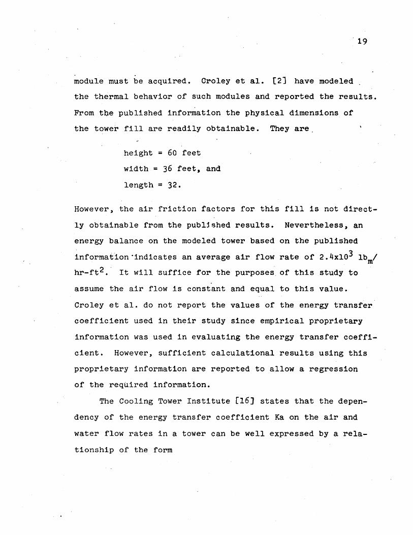
The Cooling Tower Institute [16) states that the depen-

dency of the energy transfer coefficient Ka on the air and

water flow rates in a tower can be well expressed by a rela-

tionship of the form

20

Fig. 2.3

Comparison of Reported and Predicted Mechanical Draft

Cooling Tower Performance

Water Loading = 6200 ibm/hr - ft 2

Air Loading = 1692 lbm/hr - ft2

95

90|

TowerDischargeTemp.(OF)

85

80

75

65 75

Wet Bulb Temperature (OF)

X -reported

- predicted

p p

21

Ka = aGs L1 . (2.10) -

where a depends on the fill configuration and 8 is, to a

good approximation, equal to 0.6. Using the following

expression

a = 0.065 - (T1 - 110.0)*(0.000335) T1 >90*F

and (2.11)

a = 0.0715 T. 900F

where T is the inlet water temperature, the performance1

predictions of Croley et al. based on proprietary data can

be closely matched as shown in Fig. 2.3. This value of a

is consistent with the type of fill used in modern towers

and the values of a experimentally determined by Lowe and

Christie [23].

2.3 Spray Systems

2.3.1 Literature Review

Spray cooling systems for the dissipation of waste heat

at large central power stations are a relatively new con-

cept 17J. As a consequence, the development of thermal

analysis techniques for these systems is presently incom-

plete. The development of reliable mathematical prediction

models has not been achieved and has been hindered by the

complexity of the problem.

22

As opposed to cooling towers, the water-air interfacial

area and relative air to water flow rates are not well

defined for spray systems. Open to the atmosphere, varia-

tions in the ambient wind result in different spray patterns,

different air flows through the sprays both in magnitude

and direction, and different interference effects between

the individual sprays. The spray canal system also presents

a channel hydraulics problem in that the behavior of the

water in the canal must be understood to insure optimum spray

system performance.

Porter et al.[18] [19] have authored the only two present-

ly available detailed works on the thermal performance of

spray canals. The two papers represent two different approach-

es to the problem, one analytical and one numerical. Both

models, however, are based on the same limited data which

according to the authors result in optimistic predictions [20]-

Richards of Rockford [4] have published some limited

information concerning the application of their spray modules.

They indicate that an empirical "NTU" approach is used in

the basic heat transfer calculation. Most interesting, how-

ever, is their description of the flow requirements of the

channel in which the spray modules are utilized since this

description indicates their recognition of the importance of

the channel thermal-hydraulics in the overall performance of

the system.

23

2.3.2 Selection of Model

For the purposes of survey-type analyses, the numerical

prediction of the thermal performance of spray canals as

suggested by Porter et al. [19] is most advantageous. In

this model the heat transfer ability of each spray module

is defined by an empirical "NTU" or number of transfer units

which is dependent on the ambient wind speed. The effects

of air interference between individual sprays is considered

through the use of an empirical air humidification coeffi-

cient. Given the ambient meterological conditions rad inlet

water temperature and flow rate, the calculational procedure

is to march down the canal taking into account the cooling

effect of each spray module as it is encountered. The basic

calculational algorithm is given in Fig. 2.4.

. The heat transfer equation used in the model is

C (T - T )NTU= ( n (2.12)

(h(T,.) + h(Tn2 - h(Twb)

where C = specific heat capacity of liquid water,pT = temperature of water exiting spray nozzle,n

Ts = final spray temperature,

h(T) = total heat or sigma function as defined by

Marks [15]1,

Twb = local wet-bulb temperature, and

Fig. 2.4

Computational Algorithm for Spray Canal ThermalPerformance Model (SPRANAL Program)

Pass = 1

Calculate heat transfer for upwind module

4,r4 Calculate heat transfer for next downwind module

Determine if heat transfer calculation completedfor all sprays in pass

yes

Mix cooled water with main stream to obtainspray inlet condition for next pass

Subtract evaporated flow from total flow

Determine if end of canal attained

end

24

No

I

-A

I

No

yes

-----

j

25

NTU = number of transfer units of an individual

module.

The total heat or sigma function used as the driving

potential for the energy transfer is defined by Marks [15] as

E hm - W hf (2.13)

where h = enthalpy of moist air at the wet bulb

temperature,

W = specific humidity for saturation at the wet

bulb temperature, and

hf.= enthalpy of liquid water at the wet bulb

temperature.

However, comparison of the sigma function and the enthal-

py indicates that, for the temperature range and temperature

differences of interest the following is a good approximpation;

AE(twb) Z Ah(Twb) (2.14)

where h is the enthalpy of saturated air at temperature Twb.

Since we are attempting to determine Ts by using Eq.(2.12)

and Ts is a term in the same equation an iterative solution

is necessary. The evaporated water loss is calculated using

the expression of Porter [19] It is

26

a = Cp(T - T Vig(i + B) (2.15)-

where a = fraction of water evaporated in each spray,

g = specific heat of vaporization of water, and

B = so-called Bowen ratio of sensible to evapora-

tive heat transfer.

In the application of the above equations, the Bowen

ratio can be conservatively set equal to zero, since, in

any case, the effect of water evaporation on the spray canal

thermal performance is minimal.

From the data given by Porter the relationship between

the NTU and windspeed has been deduced to be approximated by

NTU = 0.16 + 0.053*V (2.16)

where V is the windspeed in miles per hour.

In this model no direct account is made of the thermal-

hydraulic behavior of the water in the channel. However,

Porter has made some simple arguments in favor of assuming

that the channel is vertically fully-mixed between successive

passes of sprays.

2.4 Natural Draft Evaporative Cooling Towers

2.4.1 Literature Review

Conceptually, the thermal analysis of natural draft evapor-

ative cooling towers is a straightforward extension of the

27

mechanical draft cooling tower analysis developed in this

chapter. However, from a practical standpoint the problem

is considerably more complex since the heat transfer char-

acteristics and the air flow in the tower are dynamically

coupled. Also, in addition to needing to know the empirical

heat transfer coefficient of the fill, one also needs to know

the empirical air friction factors for the tower structures

and the fill. Further, a more exact determination of the

psychrometric condition of the air exiting the fill is desir-

abXe since this condition ultimat'ely determines the overall

performance of the tower.

In the past, attempts have been made, notably by Chilton[21]

to simplify the performance prediction for natural draft

evaporative cooling towers by applying an empirical relation-

ship for the overall thermal behavior. These efforts, how-

ever, were-not well received and presently the suggested

approach to the thermal analysis problem is based on a detailed

evaluation of the important physical phenomena.

Keyes [22] has outlined the necessary steps for the con-

struction of a thermal behavior model of natural draft cooling

towers. Essentially, the mathematical modeling of a natural

draft tower requires the solution of three coupled equations.

The equations are 1) an energy balance between the air and

water streams, 2) an energy transfer equation for the combined

evaporative and sensible heat transfer, and 3) an energy

28

equation for -the density induced air flow through the tower.

Keyes only reviews the general problem and discusses the

empirical information which is available for accomplishing

the modeling task.

Winiarski et al.[24] have developed a computer model

of the thermal behavior of a natural draft cooling tower

based on the three equations mentioned above. The author

notes, however, that the model presented awaits final verifi-

cation based on reliable test data from actual towers.

2.4.2 Selection of Model

The model of Winiarski et al. [24] has been chosen as the

basis for the development of a thermal behavior model of

natural draft evaporative cooling towers. The thermal ana-

lysis calculational procedure is reported in the form of a

computer program. The basic computational algorithm is given

in Fig. 2.5. The major remaining task in the model development

was, thus, the acquisition of the necessary empirical informa-

tion which would enable the computer program application. In

this regard all domestic vendors of natural draft evaporative

cooling towers were contacted and sufficient information was

obtained.

The data obtained was not typical heat transfer coeffi-

cients and air flow friction factors for a modern natural

draft tower but instead consisted of a set of typical perfor-

2Q

Fig. 2.5

Calculational Algorithm for Natural DraftEvaporative Cooling Tower Performance

Model (NATDRAFT Program)

Input data including:

atmospheric conditionspacking characteristicsdesired tower heightdesired inlet water temperaturewater loading

Estimate air flow rate

Calculate friction coefficient

Calculate heat transfer coefficient

Estimate outlet water temperature

Counterflow integration scheme

-,Is inlet water - desired value?

Yes f

Calculate pressure losses

Is calculated H - desired value? -I No

Yes

Resulting output describes tower performance

END

No

I

6

30

mance curves and tower and fill structural dimensions. Thus,

is was required to fit the computer model to the performance

curves.by a trial and error selection of appropriate heat

transfer coefficients and friction factors. The performanoe

data are known to be based on roughened-surface parallel-

plate-type tower fill with counter air/water flow. Rish [25]

has reported an empirical relationship for the heat transfer

coefficient and friction factors for smooth parallel plate

packing. They are;

C = 0.0192(L/G)0 -5 , (2.17)

and.

h C pC fG(21)L=-0.25 (2.18)

2 + 71. 6Cf($)

where Cf = friction factor,

Cp= specific heat capacity of liquid water,

G = air flow rate lbm/ft -hr,

.L = water flow rate lbm/ft 2-hr, and

h = heat transfer coefficient for evaporative

and sensible heat transfer based on enthalpy

difference potential.

It was assumed that the effect of the roughened surface of

31

the parallel plates could be simply accounted for by a fric-

tion factor multiplier F . That is;

C =F C (2.19)fa m f

where Cfa is the actual friction factor. The relationship

between the heat transfer coefficient and the friction factor

was assumed to remain the same.

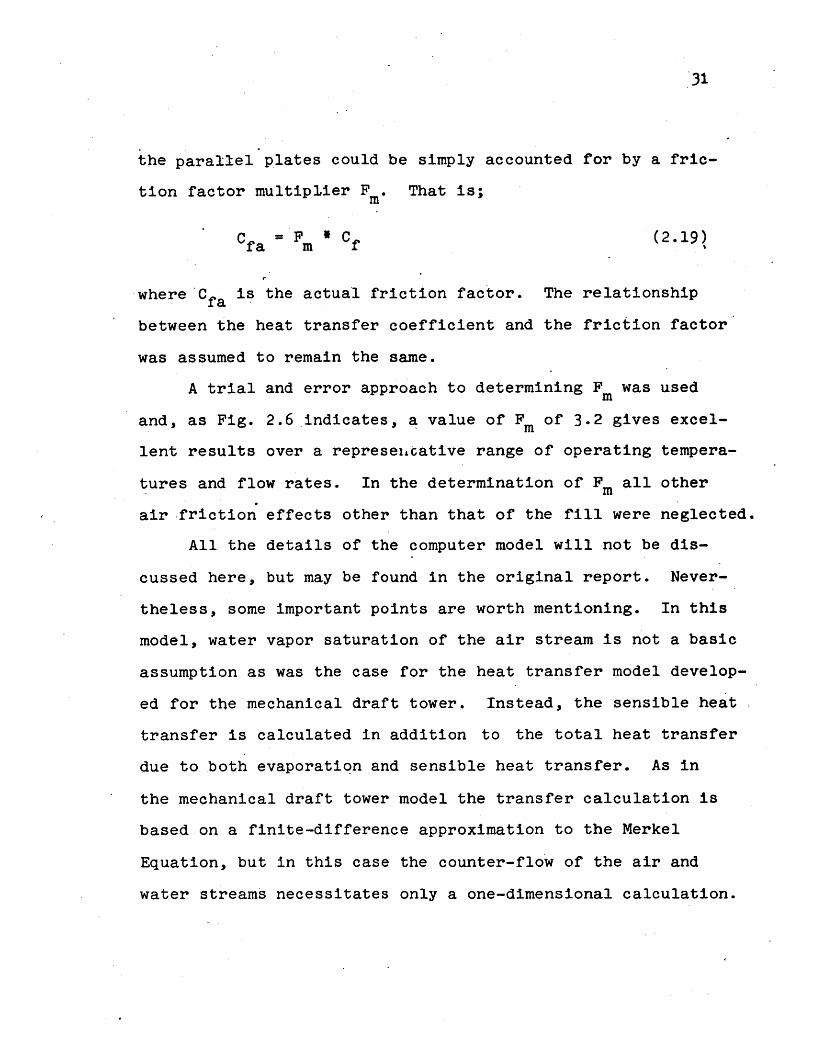
A trial and error approach to determining Fm was used

and, as Fig. 2.6 indicates, a value of F of 3.2 gives excel-

lent results over a represeAative range of operating tempera-

tures and flow rates. In the determination of Fm all other

air friction effects other than that of the fill were neglected.

All the details of the computer model will not be dis-

cussed here, but may be found in the original report. Never-

theless, some important points are worth mentioning. In this

model, water vapor saturation of the air stream is not a basic

assumption as was the case for the heat transfer model develop-

ed for the mechanical draft tower. Instead, the sensible heat

transfer is calculated in addition to the total heat transfer

due to both evaporation and sensible heat transfer. As in

the mechanical draft tower model the transfer calculation is

based on a finite-difference approximation to the Merkel

Equation, but in this case the counter-flow of the air and

water streams necessitates only a one-dimensional calculation.

32

Fig. 2.3

Comparison of Reported and Predicted Mechanical Draft

Coolina Tower Performance

Water Loading = 6200 ibm/hr - f t2

Air Loading = 1692 lbm/hr - ft2

95

90

TowerDischargeTemp.(OF)

85

80

75

55 75

Wet Bulb Temoerature (OF)

- reported

0 -predicted

33

The calculation of both the total energy transfer and.

the sensible heat t-ransfer allows the determination of the

exact psychrometric condition (both dry bulb and humidity)

of the air stream leaving each "cell" of the finite differ-

ence integration. The assumption of water vapor saturation,

if it in fact did not exist, would result in an underesti-

mate of the fill air exhaust dry bulb temperature and hence

an underestimate of the induced draft.

To complete the thermal model of a natural draft tower

a relationship between the tower height and the tower base

diameter needed to be established for different sized towers.

This was necessary because while a mechanical draft tower

may be sized to a particular cooling duty. by varying the

number of tower modules, a natural draft tower is sized by

varying the tower size. Flangan [7] has published data

concerningthe ratio of height to diameter for 16 large natur-

al draft towers which indicates an average ratio of 1.248.

2.5 Cooling Ponds

2.5.1* Literature Review

The task of mathematically modeling the thermal-hydraulic

behavior of a cooling pond is a problem which is substantially

different from the problem of modeling cooling towers. This

is because actual cooling ponds are not physically well-defined

in the sense that the important parameters which determine

34

their thermal behavior can not be assigned values which are

representative of all, or even most. cooling ponds. In

fact different cooling ponds may exhibit completely differ-

ent types of thermal-hydraulic behavior each of which require

different analysis approaches and techniques.

There are two idealized cases of pond thermal-hydraulic

behavior which yield themselves to very simple analytical

treatment [8],. These are termed the plug-flow and fully-

mixed models. In plug flow there is no mixing between the

discharge into the pond and the receiving water and the sur-

face temperature, for steady-state conditions, decreases

exponentiall-y from the pond inlet to the pond outlet. The

fully-mixed pond represents an extremely high degree of mix-

ing of the discharge and the receiving water. Thus a uni-

form temperature over the entire pond results. In reality,

the behavior of most ponds would fall between these two

extreme cases. The plug flow pond represents the best possi-

ble heat dissipation situation since the temperature of the

discharge is kept as high as possible. Conversely, the

fully-mixed pond represents a lower bound on the heat trans-

fer performance of the pond. The "worst case" performance,

however, is a short-circuited pond. For either the plug-flow

or fully-mixed model both steady-state and transient behavior

can be readily calculated.

35

Ryan [5] reported the development of a transient

cooling pond thermal-hydraulic model which was the first

attempt to realistically mathematically model the actual

physical process occurring in a cooling pond. Watanabe [6]

extended the model and reported criteria for its applicabi-

lity. This model is recommended for use as a design tool or

means of evaluating the performance of cooling ponds rela-

tive to alternative waste heat disposal systems. However,

since the model is not fully developed into a documented

computer program its applicaetion appears difficult. Also,

for the purposes of most surveys the computational time is

excessive.

2.5.2 Selection of a Model

The task of formulating a representative thermal-hydrau-

lic model of a cooling pond can be considered to be differ-

ent from the task of formulating a model of a cooling pond

which is to be used for design purposes. The present inter-

est is in mathematically representing the approximate thermal-

hydraulic behavior of a representative cooling pond. It is

perceived that this limited goal can be accomplished through

the use of a plug-flow, vertically-mixed pond model capable

of accounting for variable meterological conditions, variable

inlet temperatures, and variable flow rates. For a given

36

cooling requirement such a model would tend to predict pond

sizes which are smaller than would be normally required.

Thus, if the model were to be used in a detailed economic

comparison of alternative waste heat disposal systems the

pond economics would be unduly favored.

The vertically-mixed, plug-flow model predicts the

transient pond behavior by following a slug of water of uni-

form temperature through the pond and calculating the aver-

age heat loss for each successive day of residence in the

pond. The heat transfer correlations used in this model are

those recommended by Ryan [5] . The basic equation of the

net energy flux from a water surface exposed to the environ-

ment is

$n r - [4. Ox10~8 (Ts+460) + FW[ (es-ea) + 0.25(T-Ta]

(2.20)

where FW = 17*W for an unheated water surface,

FW = 22.4(Ae)1/3 + 14*W,

AO = Tsv - Tav (*F),

W = wind speed at 2 meters (MPH),

Tsv = virtual temperature of a thin vapor layer in

contact with the water surface,

= (TS + 460)/(l - .378 es/P),

Tav = virtual air temperature,

= (Ta + 460)/(l - .378 ea/P),

37

es= saturated vapor pressure at T (mm Hg),

ea = satu.rated vapor pressure at Ta (mm Hg),

P = atmospheric pressure (mm Hg),

Ts= bulk -water surface temperature (*F),

Ta air dry. bulb temperature (*F),

On = net heat from pond surface (BTU/day-ft2

$r = Osn + $ an = net absorbed radiative energy,

$sn = net absorbed solar radiation,

= .94($sC)(1 - 0.64C2

$sC = incident solar radiation,

C = fraction of sky covered by clouds,

. = net absorbed longwave radiation, andan

= 1.16x10- 1 3 (460 + Ta)6 (1 + 0.17C2).

The computational algorithm for the plug-flow model is

given in Fig. 2.7. Note that the model is not a perfect plug-

flow model in that each plug of water entering the pond is

assumed to be mixed with the slug immediately preceeding it.

This mixing qualitatively accounts for the effect of entrance

mixing.

2.6 Dry Cooling Towers

In relation to the other waste heat dissipation systems,

the development of a reliable performance model of dry cooling

towers is simple. The amount of heat rejected by a mechanical

draft dry tower can be shown to be directly proportional to

Fig. 2.7

Cooling Pond -Model Computational Algorithm

Assign to each discharge slug an identifi-cation number = day. of discharge

initialize slugs in pond at time zero; temp-erature, volume, fraction of volume in pond

begin calculation for day J

calculate temperature change for all slugsin pond

add discharge volume of day J to pond volume,sdt fraction of volume of slug J in pond equal

to 1

mix slugs J and J-1

determine which slugs (and fractions thereof)remain in pond by summing up slug volumes forday J, J-1, J-2, ...; until pond volume is

equaled or exceeded

determine which slugs (and fractions thereof)exhausted from pond during day J by comparingnew pond inventory (day J) and old pond

inventory (day J-1)

mix all exhausted slugs to find withdrawaltemperature for day J

end day J calculation

38

.I

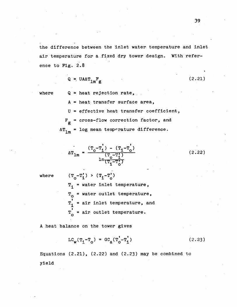
39

the difference between the inlet water temperature and inlet

air temperature for a fixed dry tower design. With refer-

ence to Fig. 2.8

Q =UAAT F (2.21)1m g

where Q = heat rejection rate,

A = heat transfer surface area,

U = effective heat transfer coefficient,

F = cross-flow correction factor, andg

ATlm= log mean temperature difference.

(T0-Ti) - (T-T )ATm T -T ) (2.22)

In 0i

where (T9-T') > (T -T')

T = water inlet temperature,

T = water outlet temperature,i

T = air inlet temperature, andi

T = air outlet temperature.

A heat balance on the tower gives

LCw(Ti-T ) = GC (T9-TI) (2.23)o a o i

Equations (2.21), (2.22) and (2.23) may be combined to

yield

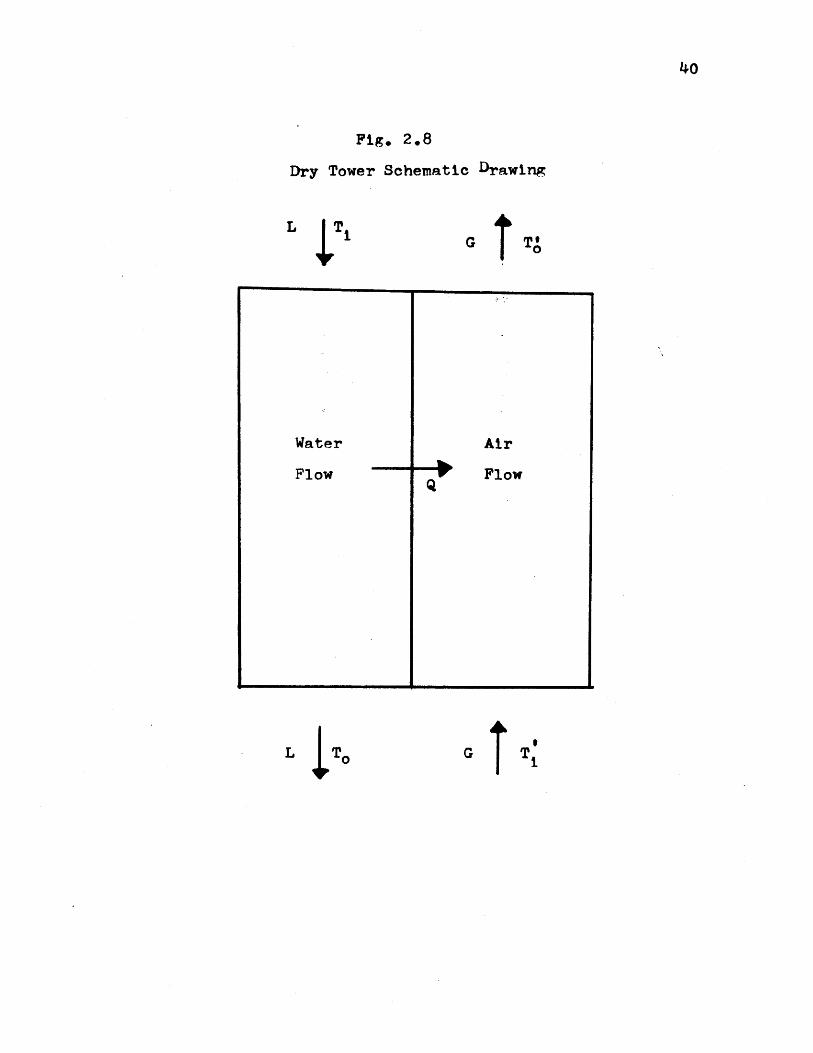
40

Fig. 2.8

Dry Tower Schematic Drawing

G

I

G5T

L T

Water Air

Flow Flow

L

41

Q ITD(ex) (2.24)e 1

GCa LCw

where ITD= T -T ,

and

x = F UA -

Now note that, for fixed values of the parameters U,

A, Fg, G and L,

Q a ITD (2.26)

This result has been found by Rossie [1] to be experi-

mentally verified. Further, Rossie has found that the ther-

mal performance of natural draft dry cooling towers may be

reasonably expressed by a relationship of the form

Q a ITDb (2.27)

where b is a constant for a given tower. A typical value of

b is 1.33.

42

REFERENCES

1.0 Rossie, J.P., "Research on Dry-Type Cooling Towersfor Thermal Electric Generation, Part 1," WaterPollution Control Research Series, EPA, 16130EE511/70.

2.0 Croley, T.E., "The Water and Total Optimizations ofWet and Dry-Wet Cooling Towers for Electric PowerStations, Iowa Institute of Hydraulic Research Report#163, Jan. 1975.

3.0 "Heat Sink Design and Cost Study for Fossil and NuclearPower Plants," WASH-1360, USA AEC, December 1974.

4.0 "Kool-Flow Spray Cooling Modules," Richards of Rock-

ford Technical Manual.

5.0 Ryan, P.J., Harleman, D., "An Analytical and Experi-mental Study of Transient Cooling Pond Behavior," MITRalph M. Parsons Lab. Report #161, Jan. 1973.

6.0 Watanabe, M., Harleman, D., "Finite Element Model ofTransient Two Layer Cooling Pond Behavior," MITRalph M. Parsons Lab. Report #202.

7.0 Flanagan, T.J., MIT Master's Thesis, 1972.

8.0 "An Engineering-Economic Study of Cooling Pond Perfor-mance," Littleton Research and Engineering Corporation,Water Pollution Control Research Series, EPA,16130DFX05/70.

9.0 "Survey of Alternate Methods for Cooling CondensorDischarge Water," Dynatech R/D Company, Water PollutionControl Reserach Series, EPA, 16130DHS11/70.

10.0 Shiers, P.F., Marks, D.H., "Thermal Pollution AbatementEvaluation Model for Power Plant Siting," MIT-EL-73-013Feb. 1973.

11.0 Merkel, F., "Verdunstungskulung," VDI Forschungsar-beiten, No. 275, Berlin, 1925.

12.0 Hallet, G.F., "Performance Curves for Mechanical DraftCooling Towers," ASME Paper #74-WA/PTC-3.

13.0 Nahavandi, A.N., "The Effect of Evaporative Losses inthe Analysis of Counter-flow Cooling Towers," UnpublishedPaper, Newark College of Engineering, Apr. 1974.

43

14.0 Yadigaroglu, G., Pastor, E.J., "An Investigation ofThe Accuracy of the Merkel Equation for EvaporativeCooling Tower Calculation," ASME paper #74-HT-59,AIAA Paper #74-765.

15.0 Marks, "Handbook of Mechanical Engineering," Chapter15, McGraw-Hill, 1968.

16.0 Cooling Tower Institute Cooling Tower PerformanceCurves, 1967.

17.0 Hoffman, D.P., "Spray Cooling for Power Plants,"Proceedings of the American Power Conference, Vol. 35,1973.

18.0 Porter, R.W., "Analytical Solution for Spray CanalHeat and Mass Transfer," ASME paper 74-HT-58, AIAApaper 74-764, July, 1974.

19.0 Porter, R.W., Chen, K.H., "Heat and Mass Transfer inSpray Canals," ASME paper 74-HT-AA, Dec. 1973.

20.0 Porter, R.W., Personal Communication, June 1975.

21.0 Chilton, H., "Performance of Natural-Draft-Water-Cool-ing Towers, Proc. IEE, 99. pt. 2, pp. 440-456, 1952,London.

22.0 Keyes, R.E., "Methods of Calculation for Natural DraftCooling Towers," HEDL-SA-327.

23.0 Lowe, H.J., and Christie, "Heat Transfer and PressureDrop Data on Cooling Tower Packing, and Model Studiesof the Resistance of Natural Draught Towers to Airflow,"International Heat Transfer Conference, Denver, 1962,pp. 933-950.

24.0 Winiarski, L.D., "A Method for Predicting the Performanceof Natural Draft Cooling Towers," EPA, Thermal PollutionResearch Program, Report #16130GKF12/70.

25.0 Rish, R.F., "The Design of Natural Draught CoolingTower," International Heat Transfer Conference, 1962Denver, pp. 951-958.

26.0 Kennedy, John F., "Wet Cooling Towers," MIT SummerCourse on the Engineering Aspects of Thermal Pollution,1972.

27.0 McKelvey, K.K., Brooke, M., "The Industrial CoolingTower," Elsivier Company, Amsterdam, 1958.

28.0 Guyer, E.C., Sc.D. thesis, "Engineering and EconomicEvaluation of Some Mixed-Mode Waste Heat RejectionSystems for Central Power Stations," MIT, 1976.

45

APPENDIX A

COMPUTER PROGRAMS FOR WASTE HEAT REJECTION

SYSTEM THERMAL PERFORMANCE CALCULATIONS

This Appendix contains FORTRAN computer programs for

predicting the thermal performance of a mechanical-drfat

evaporative cooling tower (MECDRAFT), a natural-draft evap-

orative cooling tower (NATDRAFT), and a spray canal (SPRANAL).

Programming of the cooling pond and dry cooling tower models

discussed in this report may be easily done by the user.

Tables A.l to A.3 list the required input variables for the

three programs. The FORMAT of the required input may be

easily obtained by examining the appropriate program listing.

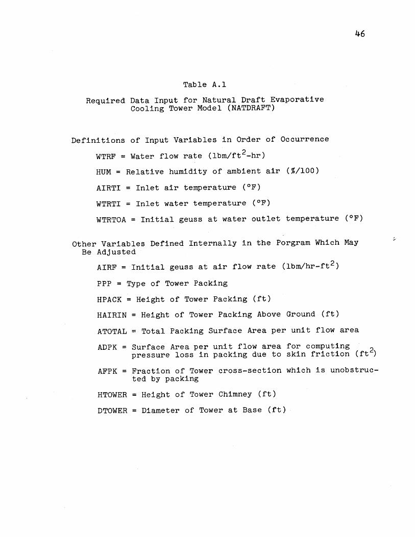
46

Table A.l

Required Data Input for Natural Draft EvaporativeCooling Tower Model (NATDRAFT)

Definitions of Input Variables in Order of Occurrence

WTRF = Water flow rate (lbm/ft2 -hr)

HUM = Relative humidity of ambient air (%/100)

AIRTI = Inlet air temperature (*F)

WTRTI = Inlet water temperature (OF)

WTRTOA = Initial geuss at water outlet temperature (OF)

Other Variables Defined Internally in the Porgram Which MayBe Adjusted

AIRF = Initial geuss at air flow rate (lbm/hr-ft2 )

PPP = Type of Tower Packing

HPACK = Height of Tower Packing (ft)

HAIRIN = Height of Tower Packing Above Ground (ft)

ATOTAL = Total Packing Surface Area per unit flow area

ADPK = Surface Area per unit flow area for computingpressure loss in packing due to skin friction (ft

2)

AFPK = Fraction of Tower cross-section which is unobstruc-ted by packing

HTOWER = Height of Tower Chimney (ft)

DTOWER = Diameter of Tower at Base (ft)

47

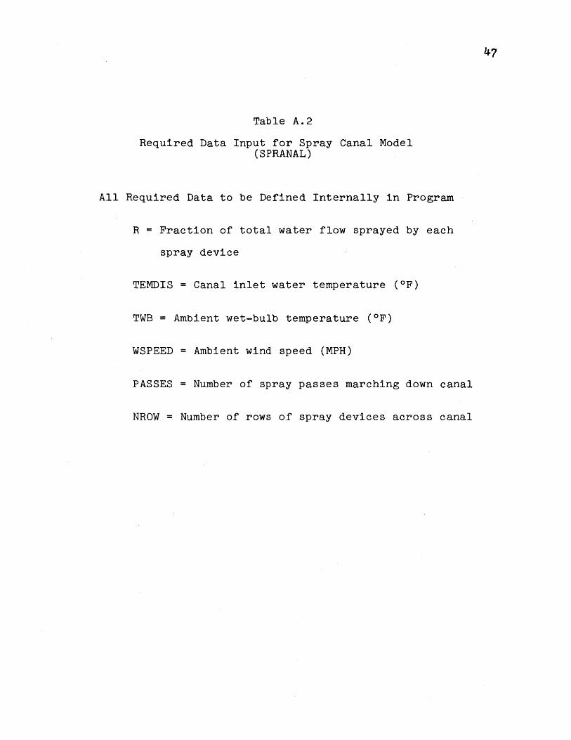
Table A.2

Required Data Input for Spray Canal Model(SPRANAL)

All Required Data to be Defined Internally in Program

R = Fraction of total water flow sprayed by each

spray device

TEMDIS = Canal inlet water temperature (OF)

TWB = Ambient wet-bulb temperature (OF)

WSPEED = Ambient wind speed (MPH)

PASSES = Number of spray passes marching down canal

NROW = Number of rows of spray devices across canal

48

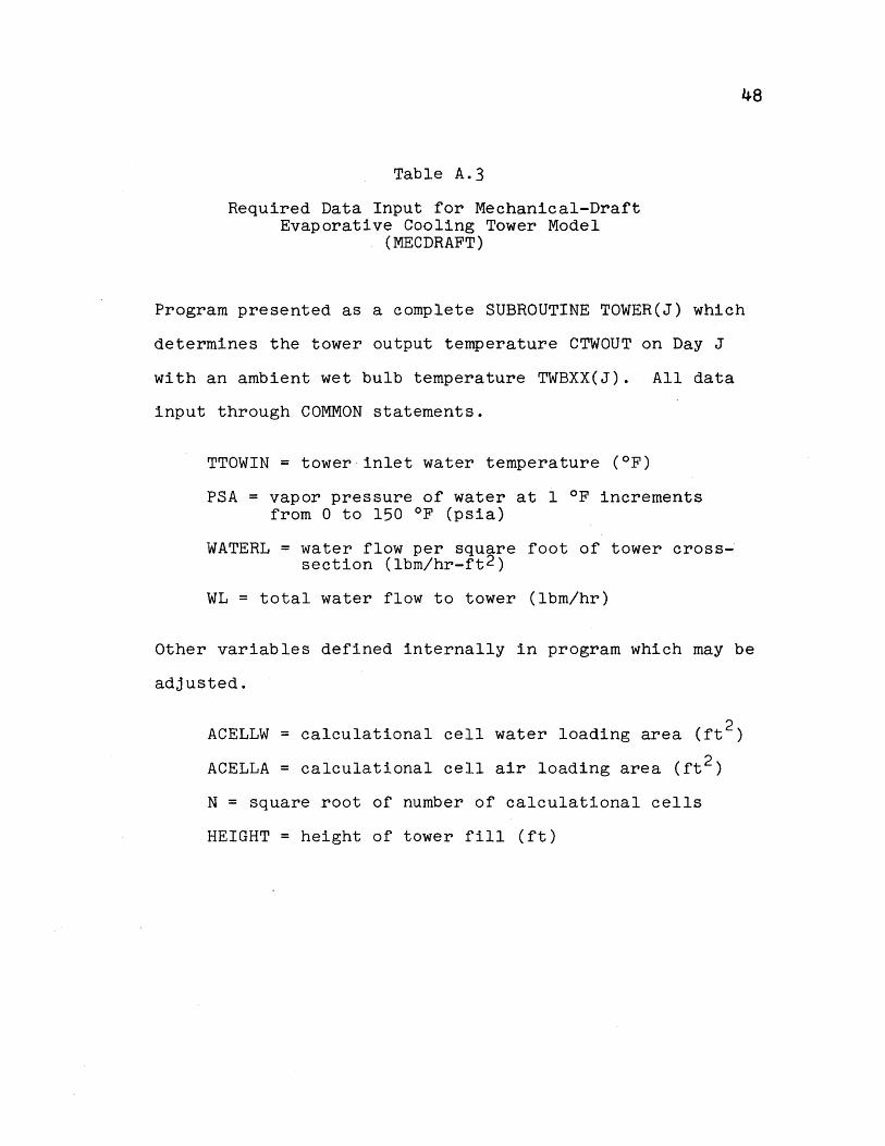
Table A.3

Required Data Input for Mechanical-DraftEvaporative Cooling Tower Model

(MECDRAFT)

Program presented as a complete SUBROUTINE TOWER(J) which

determines the tower output temperature CTWOUT on Day J

with an ambient wet bulb temperature TWBXX(J). All data

input through COMMON statements.

TTOWIN = tower inlet water temperature (*F)

PSA = vapor pressure of water at 1 OF incrementsfrom 0 to 150 OF (psia)

WATERL = water flow per square foot of tower cross-section (lbm/hr-ft2 )

WL = total water flow to tower (lbm/hr)

Other variables defined internally in program which may be

adjusted.

ACELLW = calculational cell water loading area (ft 2

ACELLA = calculational cell air loading area (ft2)

N = square root of number of calculational cells

HEIGHT = height of tower fill (ft)

--

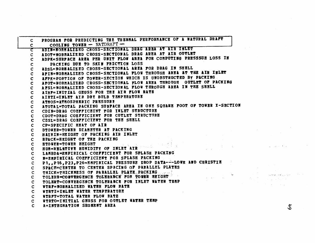
C PROGRAM FOR PREDICTING THE THERNAL PERFORMANCE OF A NATURAL DRAFT

C COOLING TOWER - NATDRAFT--C A ='. N. IZED CROSS-SECTION.L DR AREA - -IR I :T

C ADOT=NORBALIZED CROSS-SECTIONAL DRAG AREA AT AIR OUTLETC ADPK=SURFACE AREA PER UNIT FLOW ASA FOR COMPUTING PRESSSUE LOSS IN

C PACKING DUE TO SKIN FRICTION LOSSC ADSL=NORNALIZED CROSS-SECTIONAL AREA FOR DRAG IN SHELL

C AFIN=NORNALIZED CROSS-SECTIONAL FLOW THROUGH AREA AT THE All INLET

C AFPK=PORTION OF TOWER-SECTION WHICH IS UNOBSTRUCTED BY PACKING

C AFOT=NORMALIZED CROSS-SECTIONAL FLOW AREA THROUGH OUTLET OF PACKING

C AFSL=NORNALIZED CROSS-SECTIONAL FLOW THROUGH AREA IN THE SHELL

C AIRF=INITIAL GEUSS FOR THE AIR FLOW RATEC AIRTI=INLET AIR DRY BULB TEMPERATUREC ATMOS=ATMOSPHERIC PRESSUR!C ATOTAL=TOTAL PACKING SURFACE AREA IN ONE SQUARE FOOT OF TOWER X-SECTION

C CDIN=DRAG COEFFICEINT FOR INLET STRUCTUREC CDOT=DRAG COEFFICIENT FOR CUTLET STRUCTUREC CDSL=DRAG COEFFICIENT FOR THE SHELLC CP=SPECIFIC HEAT OF AIRC DTOVER=TOWER DIAMETER AT PACKINGC HAIRIN=HEIGHT OF PACEING AIR INLETC BPACK=HEIGHT OF THE PACKINGC HTOVER=TOVER HEIGHTC HUM=RELATIVE HUMIDITY OF INLET AIRC LANBDA=EMPIRICAL COEFFICIENT FOR SPLASH PACKINGC N=EMPIRICAL COEFFICIENT FOR SPLASH PACKINGC P1,,P16,P23,P26=EMPIRICAL PRESSURE DROP DATA---LOWE AND CHRISTIEC SPACE=CENTER TO CENTER SPICING OF PARALLEL PLATESC THICK=THICKNESS OF PARALLEL PLATE.PACKINGC T OLERR=COTIERG ENCE TOLER-A*Cl FOR TOW IEIGHTC TOLERT=CONVERGENCE TOLERANCE FOR INLET WATER TEMPC WTRF=NORMALIZED WATER FLOW RATEC WTRTI=INLET WATER TEMPERATUREC WTRFT=TOTAL WATER FLOW RATEC WTRTO=INITIAL GEUSS FOR OUTLET WATER TEMPC A=INTEGRATION SEGMENT AREA

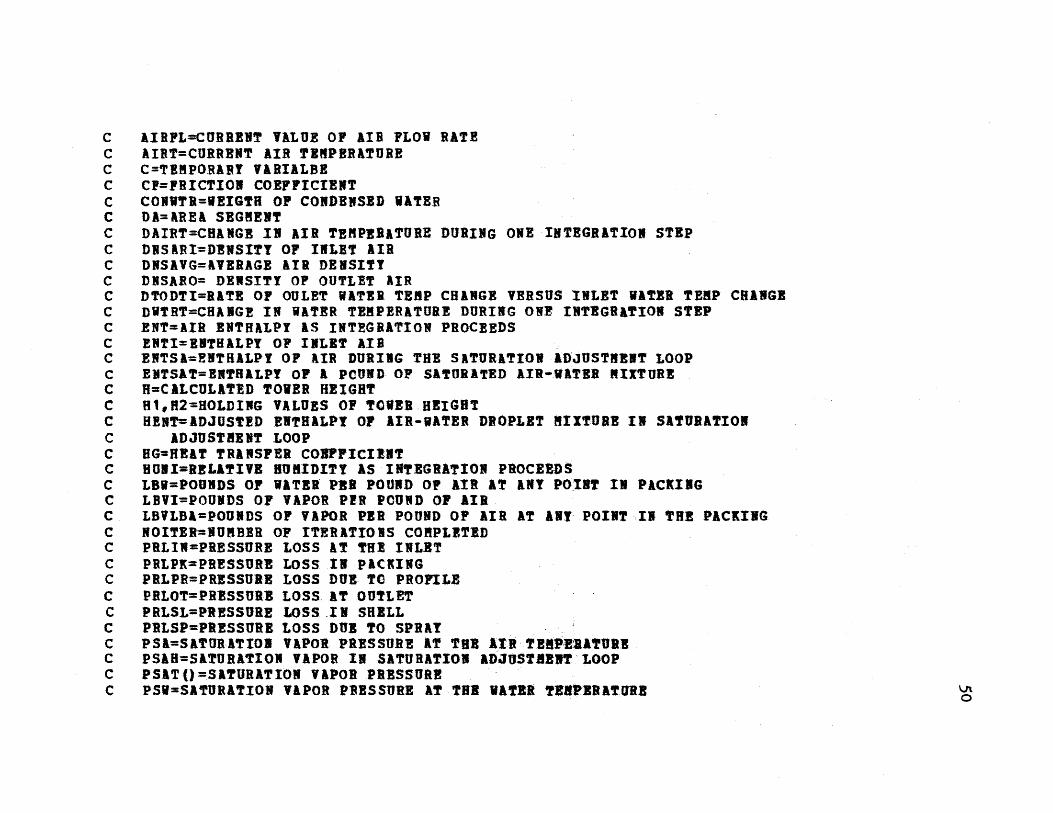
C AIRFL-CURRENT VALUE OF AIR FLOW RATEC AIRT=CURRENT AIR TEMPERATUREC C=TEMPORABY VARIALBEC CF=FRICTION COEFFICIENTC CONTR=VEIGTH OF CONDENSED WATERC DA=&REA SEGMENTC DAIRT=CHANGE IN AIR TEMPERATURE DURING ONE INTEGRATION STEPC DNSARI=DENSITY OF INLET AIRC DNSAVG=AVERAGE AIR DENSITYC DNSARO= DENSITY OF OUTLET AIRC DTODTI=R&TE OF OULET WATER TEMP CHANGE VERSUS INLET WATER TEMP CHANGEC DWTRT=CHANGE IN WATER TEMPERATURE DURING ONE INTEGRATION STEPC ENT=AIR ENTHALPY IS INTEGRATION PROCEEDSC ENTI=ENTHALPY OF INLET AINC ENTSA=ENTHALPY OF AIR DURING THE SATURATION ADJUSTMENT LOOPC ENTSAT=ENTRALPY OF A PCUND OF SATURATED AIR-WATER MIXTUREC H=CALCULATED TOWER HEIGHTC H1,H2=HOLDING VALUES OF TOWER HEIGHTC HENT=ADJUSTED ENTHALPY OF AIR-WATER DROPLET MIXTURE IN SATURATIONC ADJUSTMENT LOOPC HG=HEAT TRANSFER COEFFICIINTC HUNI=RELATIVE HUMIDITY AS INTEGRATION PROCEEDSC LBW=POUNDS OF WATER PER POUND OF AIR AT ANY POINT IN PACKINGC LBVI=POUNDS OF VAPOR PER POUND OF AIRC LBVLBA=POUNDS OF VAPOR PER POUND OF AIR AT ANY POINT IN THE PACKINGC NOITER=NURBER OF ITERATIONS COMPLETEDC PRLIW=PRESSURE LOSS AT THE INLETC PRLPK=PRESSURE LOSS IN PACKINGC PRLPR=PRESSURE LOSS DUE TO PROFILEC PRLOT=PRESSURE LOSS AT OUTLETC PRLSL=PRESSURE LOSS IN SHELLC PRLSP=PRESSURE LOSS DUE TO SPRAYC PSA=SATURATION VAPOR PRESSURE AT THE AIR TEMPERATUREC PSAH=SATURATION VAPOR IN SATURATION ADJUSTEENT LOOPC PSATO=SATURATION VAPOR PRESSUREC PSV=SATURATION VAPOR PRESSURE AT TUE WATER TENEfRATURE

- -1-,,-,-- -4-

C VHSP=VELOCITY HEADS LOST DUE TO SPRAYC VHVC=VELOCITY HEADS LOST DUE TO TENA-CONTRACTA IN THE TOWERC VIN=AIR INLET VELOCITYC VNON=NONINAL VELOCITY IN PACKINGC VPEN ENTHALPY OF MOISTURE IN AIR, USED IN SATURATION ADJUSTMENT LOOPC VPENT=ENTHALPY OF VAPOR IN AIRC VPRES=VAPOR PRESSURE OF AIRC VPK=AIR VELOCITY IN PACKINGC VOT=AIR VELOCITY AT OUTLETC VSL=AIR VELOCITY IN THE SHELLC WTRLT=VATER WHICH COWDENSES OUT DDRI5G N INTEGRATION STEPC WTRT1,VTRT2=HOLDS WATER INLET TEMPERATURE FOR EXTRAPOLATIONC LOGICAL VARIABLESC ENDFLG= TRUE IF PROGRAM HAS REACHED NORMAL TERMINATIONC EXTIFL=TRUE IF ITERATION IS BEING HADE TO EXTRAPOLATE AIRFLOWC EITTO=TRUE IF ITERATION IS BEING MADE TO EXTRAPOLATE OUTLET WATER TEMPC PPP=TRUE IF TOWER HAS PARALLEL PLATE PACKINGC PRII=TRUE IF SPLASH PACKINGC PRITER=TRUE IF RESULTS OF EACH ITERATION ARE TO BE PRINTEDC PRSTEP=TRUE IF EACH STEP IN ITERATION IS TO BE PRINTED

LOGICAL ENDFLG, PRITER, PRSTEP, EXTITO, EXTAFLLOGICAL PPPREAL LBVLBALBWLANEDAN,LBVLBSLBVIKAL

1111 CONTINUEREAD(5,999) VTRF,HUMAIRTI,WTRTIWTRTOA

999 FORMAT(5F10.3)FACTOR=3.2

1001 CONTINUEVTRTO=WTRTOAAIRF=1264.0

C**** ***************************************************************************

C IMPORTANT### SET PPP TRUE IF PARRALLEL PLATE PACKING IS USEDC IF PPPP IS TRUE RISH'S HT TRANSFER AND PRESSURE DROP REALATIONSC ARE USEDC*******************************************************************************

PPP=. TRUE.I-b

RPACK=5.33HAIRIN=35.6

C SKIP THE NEXT INPUT PARANETERS IF PARRALLEL PLATE PACKING IS USEDIF(PPP) GO TO 2LANBDA=0.065N=.6P 13=1.2P16=0.9P23=2.0P26=1.3ATOTAL=HPACK

2 CONTINUE

C IF PPP IS TRUE INPUT ATWCER AND APPK AS REQUIREDC *******************************************************************************

IF(.NOT.PPP) GO TO 7ATOTAL=204.6ADPK=204.0AFPK=.70

7 CONTINUECP=0.24ATROS=14.4AFIN=1.0AFOT=1.0AFSL=1.0ADIW=0.0ADOT=0.0ADSL=0.0CDOT=0.0CDSL=0.0CDIN=0.0TOLERT=0.3TOLERH=10.0HTOVEWR=51 4.0

DTOVER=372.0STEPS=2Q .0LS?1P-50LP§DFLG *FALSE.

PRITRR=.TRE.PESTEP=. FALSE.EXT WC *FALSE.

EXT &FL-=.FALS2.L1TER=52-AIR?= AIR?!W0ITh'=0VHYC0. 167* (DTOVER/HAI.RlU)**2VPRES=HUM*PSA? (AIR?)LBVLBA=0 .622*VPRES/ (AIMOS-VPRES.)VPZNT=l06l1.04. 44*AIRTIWI=CP* (AIRT- 32.0) *VrEI1*LBVLE+AVPR9S I=VPRESLBVI=LBVLBADWSA RI= ( (ATMOS- VPRES) /53. 3 VPPlS/85 7)+ *1414wO/ (#60.-04&IiT)DA=ATOTAL/STBPSAIRFL=0,0

CC END INPUT! AND INITIALIZATIONC START ITERATIONC

95 VNOB=AIRP/ (DNSARI*3600.0)VHSP=0. 16*HRIRIV* (WTRP/AIRF) **1 .32IF-(PPP) GO TO 16K&L-HPACK*LAIBDA* (AIRI/VTRF) **Jf

GCP*WTRF*KAL/HPACKHGOUT=0 .0Tl=VN0t /3.0-1 .0Pl-(P16-PI3) *Tl+P1.3P2= (P26-P23) *T14.P23

VHLPK=((P2-P1)*(WTRF-1000.O)/1000.O+P1)*HPACKcp=oo*GO TO 15

16 CP=O.0 192* jVTRP/AIRF) **O.5CF=PACTOR *CFHG=CP*AIR*CF/(2.OtCP*71,6* (AIRP/ VTRF) **O.25)K&AL5.G*ATOTAL/ (CP*WTRY)HGOUT=HG

15 NTRTM-TRTOEu'r=ENTIHUftI=HollA=0.0LBVLBA=LBVIVPRBS=VPRES ICOweri=o. 0AIRT= AIBTI

c INTZGRATION LOOP BEGINS VITH STAT~EENT 6

6 PSW=PSAT(VTRT)IV(PSW.BQ.O.0) GO TO 110RWTSAT=CP* (WTRT-32.O) +(1061.O+.44#*1RT) :*O,.622*PSV/(ATNOS-PSV)C=HG*Dk* (ENTS AT-ENT) /CPIF(. NOT. PlSTEP.OR.lXTVTO.OR.E?!AFL) GO TO .35IP(LSTIPLT.47) GO T.9 ~

37 PORSAT(52H1COOLING, TOVEtt PROGRAM BYTE E STEP RESULTS-OF ONEw1 10Hi ITERATION/57H0 V&TER AIR SATUE ACTUAL EEL PNDS V2TR/ VAPOR/56f AREA TYEMP TEMP ENTHAL ENTHAL HUN PIDS AIR3PRES)

LSTZP=0LITER=52

36 LSTEP=LSTEP+1WRITE(6,38) AuWTRTiAIRTENTISATuENTgHUNIuLBVLBAerVPRES

38 FORMAT (5F7. I, F6. 3 ,F9 *5 vF7 * 4)35 DVTRT=C/VTRF 4r

DENT=C/AI RFD AIRT=HG*Dk* (WTRT- AIRT) / (AIRF*CP)VTRT=WTR T+DWTRTENT=ENT+DENTAIRT=AIRT+DAIRTA=A+DAVPENT=1061.0+0.444*AIETLBVLB A=(ENT-CP* (AIRT- 32.0)) /VPENTPSA=PSAT (AIRT)IF(PSA.BQ.0.0) GO TO 110LBVLBS=0.622*PSA/(ATNOS-PSA)HUNI=LBVLBA*(0.622+LBVLBS)/(LBVLBS*(.622+LBVLBA))VPRES=HUI*PSA ,IF(HUNI.LE.1.0) GO TO 99

C IF MIXTURE IS SUPER-SATURATED, FIX-UPC**** ******** ******************* ***** *******************************************

T= AIRT97 T=T+O.1

PSAH=PSAT(T)IF(PSAH.EQ.0.0) GO TO 110VPEN=1061.0+.444*TLBW=0.622*PSAH/( TMOS-PSAH)ENTSA=CP* (T-32.0) +VPEN*LBWHENT= (LBVLBA-LBV+CONWTR) * (T-32.0) *ENTSAIF(ENT.GT.HENT) GO TO 97CONWTR=LBVLBA-LBV+CONWTRENT=ENTSAAIRT=?

99 IF(A.LT.ATOTAL) GO TO 6

C END INTEGRATION SECTIONCC COMPUTE PRESSURE LOSSES FOR THIS ITERATION

100 IF(EXTVWTO) GO TO 24.

YPBNT= 1061.0+0.444*AIRTLBVLBA= (ENT-CP* (AIRT- 32.0)) /VPENTVTRLT=AIRF* (LBTLBA+CONVTR -LBVI)VPRES=LBVLBA*ATNOS/(0.622+LBVLBA)DWSARO= ((ATMOS-VPRES)/53.3+VPRES/85.7) *144.0/(460.0+IRT)DNSARO=DNSARO*(1.O+CONTR)/(1.0+CONVTR*DNSARO/62.4)DNSAVG= (DNSAIRI+DNSARO)/2. 0VIN=VNOM/AFINVOT=AIRP/(DNSARO*APOT*3600.0)VSL=AIRF/(DNSARO*APSL*3600.0)PRLIN=CDI N*DNSARI*0 .0 16126*ADIN*VIN**2IF(.NOT.PPP) GO TO 102VPK=AIRP/(DNSAVG*AFPK*3600.0)PRLPK=CF*DNSAVG*0.016126*ADPK*VPK**2GO TO 103

102 PRLPK=DNSARI*0.016126*VHLPK*VNO0**2VPK=VNOM

103 PRLOT=CDOT*DNS&RO*0.0 16126*ADOT*VOT**2PRLSL=CDSL*DNS ARO*0.0 16126*ADSL*VSL**2PRLVC=VHVC*DNSARI*0.0 16126*VNOH**2PRLSP=VHSP*DNSARI*0.O 16126*VNON*VNONPR LPR=PRLOT+PRLIN+PRLSLH=(PRLPR+PRLPK+PRLSP+PRLVC)/ (DNSARI-DNSARO)IF(ENDYLG) GO TO 40NOITER=NOITER+1IP(.NOT.PRITER.OR.EXTAL) GO TO 21

40 IF(LITER.LT.52) GO TO 30LSTEP=50LITER=OWRITE (6,31)

31 FORMAT(46H1COOLING TOVER PROGRAM - RESULTS OF ITER&TIONS/I 221, 17HAIR CALC TOWER/263H OUTLET VELOTY HEAT CHARAC- SKIN INLET3, 50H OUTLET OUTLET PROFILE PACKING SPRAY VENA CON/463H ITER WATER AIR IN TRANS TERISTIC FRICTION RELAT WATER5, 56H AIR AIR PRESSURE PRESSURE PRESSURE PRESSURE TOWER/

663H NO LOSS DENSITY PAKING COEFF (K*A/L) COEFF HUMID TEMP7, 57H TEMP ENTHAL LOSS LOSS LOSS LOSS HEIGHT)

30 WRITE(6,32)NOITER,WTRLTDNSAROVPKRGOUTKALCF,HURI,WTRTAIRT,1 ENTPRLPRPRLPK,PRLSPPRLYC,H

32 FORMAT(1HOI4,F7.2,F8.6,F7.3,F6.3,F8.4,F9.5,77.3,F6. 1,1 F6.1,F7.1,F0.6,3F9.6,F7.0)

LITER=LITER+2IF(ENDFIG) GO TO 33

C END PRINTING RESULTS OF ONE ITERATION

21 IF(NOITER.LE.100) GO -tO 39WRITE (6,98)

98 FORMAT(47H MORE THAN 100 ITERATIONS. EXECUTION TERMINATED)GO TO 39

C ITERATION STOP BYPASSEDSTOP

C NOW FIND IF SPECIFIED TOLERANCES ARE NET

39 IF (ABS (WTRT-WTRTI) .LE.TOLERT) GO TO 27IF(.NOT.PRITER) GO TO 46IF(.NOT.EXTAFL) GO TO 48WRITE (6,42) WTRTO

42 FORMAT(30H (EXTRAPOLATING FROM VTRTO=,F. 1, iH))LITER=LITER+1GO TO 46

48 VRITE(6,43) WTRTOLITER=LITER+2

43 FORNAT(31H (EXTRAFOLATING FROM VTRT0=,F6.1,1H))46 WTRT1=UTRT

WTRTO=WTRTO+O.1EXTVTO=.TRUE.GO TO 15

27 IF (EX TAFL) GO TO 50IF(ABS(H-HTOWER).LE.TCLERH) GO TO 29

IF(.NOT.PRITER) GO TO 44WRITE(6,41) AIRFLITE=LITER+2

41 FORMAT(26H0(EXTRAPOLATING FROM AIRF=,F7.1rlH))44 AIRFL=AIRF

H 1-=RAIR?= A IR+ 10. 0EXTAFL=.TRUE.GO TO 95

C A SAMPLE ITERATION HAS BEEN MADE TO ADJUST AIRF OR VTRTO

50 H2=HDAFDH=10.0/(H2-H1)EXTAFL=.FALSE.AIRF=AIRF+DAFDH* (HTOIR-5)I?(.WOT.PRITER) GO TO 95WRITE (6, 55) AIRFLITER=LITER+ I

55 FORMAT(20H (MODIFYING AIRF TO ,?7.1,1H))GO TO 95

24 VTRT2=WTRTDTODTI=0. 1/(WTRT2-WTRT 1)EXTVTO=.FALSE.UTRTO1=VTRTOWTRTO=VTRTO+DTODTI*(INYRTI-WTRT)IF(.NOT.PRITER) GO TO 15IF(.WOT.EXTAFL) GO TO 62WRITE(6,61) WTRTO

61 FORMAT(25H (MODIFYING RTRTO TO P?6.1t18))LITER=LITER+1GO TO 15

62 WRITE (6,60) WTRTOLITER=LIT ER+2

60 FOREAT(21H (MODIFYING UTRTO TO ,F6.1,1R))GO TO 15

29 IF(PRITER) GO TO 33ENDFLG=.TBUE.LITER=52GO TO 100

33 WRITE(6,96)UTRTO, H96 FORNAT(26H END COOLING TOWER PROGRAN/34HOFINAL OUTLET WATER TEMP

1ERATURE ISF6.1/22HOFINAL TOWER HEIGHT IS,F7.0)WRITE(6,1002) FACTOR

1002 FORNAT(8H FACTOR=,F10.4)RAVGE=WTRTI-W TRTOWRITE (6, 998)

998 FORMAT(102H WATER LOAtING HUMIDITY INLET AIR TEMP INLE

IT WATER TEMP ACTUAL OUTLET UATER TEMP RANGE)WRITE (6,997) WTRFRUNAIRTI,NTRTI, WTRTOA, RANGE

997 FORMAT (2XF1O.3,6XF1O.3,6XF10.3,8,F1O.3, 13XF1O.3, 1,F1O.3)GO TO 1111STOP

110 AIRF= (AIRF-AIRFL)/2.04&IRFLIF(.NOT.PRITER) GO TO 95WRITE(6,111) AIRFLITER=LITER+2

111 FORMAT (19HO(ADJUSTING AIRF TO,7.1, 15H FOR STABILITY))GO TO 95ENDFUNCTION PSAT(T)DIMENSION V(181)DATA M/0/

D ATAV/.08854,. 09223,.09603,.09995,.10401, .10821,.11256,. 11705,. 121170,. 12652,. 13150,. 13665,. 14 199,. 14752,. 15323,. 159 14,. 16525,. 17157,2.17811,.18486,.19182, .19900,.20642,.2141, .2220,.2302,.2386,. 2473,.32563,.2655,.2751,.2850,.2951,.3056,.3164,.3276,.3390,.3509,.3631.43756,.3886,.4019, .4156,.14298,.4443,. 4593 .747,.4906,.5069,.5237,.55410,.5588,.5771,.5959,.6152,. 6351,.6556,. 6766,.6982,.7204,.7432,.67666,.7906,.8153,.8407,.8668,.8935,.9210,.9492,.9781,1.0078,1.03827, 1. 0695, 1. 10 16, 1. 1345, 1. 1683, 1. 2029,1.2384,1.2748, 1.3 121, 1.3504, 1.83896, 1. 4298, 1.4709, 1.5130, 1.5563, 1. 6006, 1.6459, 1. 6924, 1.7400, 1.788

98, 1.8387, 1.8897, 1.9420, 1.9955,2.0503, 2.1064,2.1638,2.2225, 2.2826, 2*.3440,2.4069,2.4712,2.5370,2.6042,2.6729,2.7432,2.8151,2.8886,2.96*37,3.0404,3.* 1188,3. 1990,3.281,3.365,3.450,3.537,3.627,3.718, 3.811,

*3.906,4.003,4.102,4.203,4.306,4.411,4.519,4.629,4.741,4.855,4.971,*5.090,5.212,5.335,5.46l,5.590,5.721,5.855,5.992,6.131,6.273,6.471,*6.565,6.715,6.868,7.024,7.183,7.345,7.510,7.678,7.850,8.024,8. 202,

*8.383,8.567,8.755,8.946,9.141,9.339,9.541,9.746,9.955, 1O168,10.38

*S,10.605,1O.830,11.058,11.290,11.526,11.769,12.011,12.262,12.512,1*.771,13.031, 13.300, 13.568, 13.845, 14. 123, 14.4110, 14.696/

NT=TPSAT=O.OIF(NT.GT.31) GO TO 5PSAT=V(1)WRITE(6,2) T

2 FORIAT(36HOERROR IN PSAT: TABLE EXCEEDED. T=,?8.2)4 M=N+1

IF(.LB.50) RETURNWRITE (6, 3)

3 FORNAT(53H0 MORE THAN 50 ERRORS IN PSAT - EXECUTION TERMINATED)STOP

5 IF (NT.GE.212) GO TO 41 PSAT=V(NT-3 )+(Y (WT-30)-V(NT-31))*(?-NT)

RETURNEND

C PROGRAM FOR PREDICTING THE THERMAL PERFORM NCE 0 SPRA SPRANAC E=TOTAL WATER EVAPORATEDC ALPHA=FRACTION OF WATER EVAPORATEDC F=AIR INTERFERENCE FACTORSC PSA=SATURATION VAPOR PRESSUREC TBIX=MIXED CANAL TEMPERATUREC TST=SPRAY TEMPERATUREC TVBL=LOCAL WET BULB TERPERATUREC PASSES=NUMBER OF PASSES MARCHING DOWN CANALC NRON=NUMBER OF SPRAYS ACROSS CANALC R=FRACTION OF WATER SPRAYED BY EACH SPRAYC TEMDIS= CANAL INLET TEMPERATURE

0

SSVd, 03VaI HiOJ KOIJlflf!31VD liISIRO=I

BOU I=AovuaL**L=MJLVd

slawal= W) Iia***s.~l1IA idhI****=AOvff

*****ILnVd~ldH****=81J.~f

~ 1LfidMi*****=sictaj;**.**fl'VA JdidII.****=H

96*0=(S) AtitaiO= (t)a

8t o=(Z) I

82180~d 10 CalIIOd~g SV SZO'IVA aL

VSd (S'raVZS849aMddgE .1VZV

sassva RRORIMI(Oooo) J(00O~ihoaijl(ooooa)jLsL O(oor)xii~l loisiauio

(OSO)VSd ikoismavia(00Ja'(OOZ*oi)Vea'IV*(OOZ)R KOISHRUIG

anivYadNRaSHVHZ3SIa IVfVDZ=LI'IZZON I V AV~dS JO aHOIVHadUlI=*Z D

smoILvigLI ao Ra~0waK=aIflI 3m~l agnaadwaJ. IV ldIveJlgz=LH 3

HaRM SSVd=l aoijD1Iu kaaoo=a 0

a3JdS UMIEOS(12dSftzanivaazwai aing zaAagi 3

1=1+ IC BEGING PASS CALCULATION WITH UPWIND NODULE10 J=J+l

IF(IEQ.1) TWBL(J#.r)=F(J) (Tfil 1 (1) -TWB) +TWBIF(I.GT.1) TVBL(J,,I)=P(J)*.(TRIX(1-1)-TVB)+TVB

NTU=O. 16+ (0.053) *WSPEEDIF(r.EQ.1) TW=TRIX(l)IF(I.GT.1)TS--TN-30.0ITVBL=TVBL (JI, I)ITVBLI=ITWBL*lPSATBI=PSA(ITWBL)PSATB2=PSA (IT'VBLI)ITN=TgITNI=ITN+lPSATNI=PSR(TTN)PSATV2=PSA(lT*l)TITN=ITNTITVBL=ITVBLPSATN=PSATNI+ (TV-TITV)'* (P5k-T52-PSATV.l),,-.;.PSATVB=PSATS14-(TlBt!IJ't':t), ;IITVB'L 'f.P AT824' KTBI)HTN=0,935*(O.o24*TW+(-ow622*PSATN/-(14*7-PS ATN))*0061,8+0e44*TY))HTVBL=0.935*(0.24*?VB.L(Jol )+(Oo622*PSATVB/(14.7-PSkTWB))-

I *(1061,8+0.44*TVBL(Jrl.)))ITR&TZ=0

C BEGIN ITERATICN FOR HEAT TRANSIFE18. CCALCUL:AT1611'30 TS&VE=TS

ITRATZ=ITRATB+ IITS=TSITSI=ITS+l

PSATS I =PSA (ITS)PSATS2=PSA (ITS 1)

TITS=ITSPSATS=PSATS1+(TS-TITS)*(PSkTS2',p 1. '1HTS=0.935*(0.24*TS+(O 0622*PSATS/(14..7-- PSi-'At.t))..*(1061.8+0,44*TS))TS=TN-NTU*((HTS+HTN)/,2.0-HTUBL),

log IIU3 ost8 OJl 05

osI. ox o!) (sassvdeoabi)aianuiJmioD 001

((Awi1 )d'vw a(I 'I) J.ta-M1x/I i ) W I I I((I~n~-1*soI'll)V 8 fl*8i*10If l-ItLoa-ot ) (I) lt

aouvt='iw 001 Octoo = (I) lKimJ

(E'SLJ* SI 21CZOJVdURJ. GRINl LKSRHd an~ HtE)Lvlaaoi ZL

L 1 xI (oa 0 Sol ux) Ji

ooo=(tOa (os~a;a)ai

(i'x) VHd1lV+VHd IV1--V HdTIJaoumst= i OL oa

0 0=vHdTvI102I1R03 09

SS~d H3U U0i SISSO'I RAUV8oodvAa aaROS 3

09 oa. os (moax*0ir)aI(E*Sti SI WElDI I

S.S~d 011 IJOL"EI 808 IV Ra103 cIo VddS alll H8l)LYII)Is

OE 01 09

os 03; of) (tioovuazxo)&(s-L-ZAVS.) sGv=ULLJIUa

TCC=TMII(I)160 CONTINUE

WRITE(6,175) TCC175 FORMAT(36H CANAL DISCHARGE TEMPERATURE EQUALS ,F15.3)

STOPEND

C THIS PROGRAM PREDICTS THE THERMAL PERFORMANCE OF EVAPORATIVEC MECHANICAL DRAFT COOLING TOuERS-- ECDAFT-C KAL=KA/LC JKEEP=RETAINS VALUE OF JC TWI= TOWER INLET TNMPERATUREC ALPHA=PACKING EMPIRICAL COEFFICIENTC BETA=EMPIRICAL PACKING COEFFICIENTC AIRG=AIR LOADING LB/HR-FT**2C ACELLW=NORALIZED CALCULATIONAL CELL WATER LOADING AREAC ACELLA=NORNALIZED CALCULATIONAL CELL AIR LOADING AREAC RLG ==RATIO OF WATER FLOW TO AIR FLOW IN EACH CELLC NOITT=NUNBER OF ITERATIONSC N=SQUARE ROOT OF NUMBER OF CELLSC HEIGHT=HEIGHT OF PACKINGC GNTU=KA/LC FNTU=KAV/AIRGC DNTU=NTU PER CELLC TO=OUTLET WATER TEMPERATUREC PS=SATURATED VAPOR PRESSURE AT TOWER WATER INLET TEMPERATUREC H=ENTHALPY OF NIOST AIR AT WATER TEMPERATUREC TS=SATURATED VAPOR PRESSURE AT SPECIFIED METR. CONDITIONC HA=ENTHALPY OF moIST AIR AT SPECIFIED METR.CONDITIONC J=NUMBER OF ROW ACROSS, I=TOP ROWC I=NUEBER OF ROW ACROSS, I=AIR INLET SIDEC TI=WATER TEMPERATUREC HW=MOIST AIR ENTHALPYC KC=ITERATION NUMBER CHECKC TV2=TEMPERATURE OF WATER AT THE EXIT OF AN INCRSENT(CEL)C TWBAL=TEMPERATURE OF AIR AT TOWER EXITC DH=ENTHALPY DIFFERENCE OF THE AIR BETWEEN THE INLET AND OUTLET OF A CELL

A, I

C DH1=ENTHALPY DIFFERENCE BETWEEN WATER AND AIR ENTERING A CELL

C HA2=ENTHALPY OF HOIST AIR AT THE EXIT OF A CELLC THIS PROGRAM HAS INCLUDED THE VARIOUS PARAMETER VALUES FOR THEC FOLLOWING TOWERC FILL WIDTH=36 PEET (INCLUDES BOTH SIDES)C FILL HEIGHT=60 FEETC UNIT FILL LENTH=32 FEETC PAN DIAMETEB=28 FEET

SUBROUTINE TOWER(J)DIMENSION TWBIX (380) ,CTWOUT (380)DIMENSION HW(30)v, TW(30), PSA(150)COMMON/TOWTEM/TTOWINCOMBO N/VET/TWBXXCOmMON/EFF/CTWOUTCONON/ATMOS/PSACOMMON/WATER/WATERLWIREAL KALJKEEP=JTWB=TVBXX (J)TWI=TTOWIN

53 CONTINUEALPHA=0.065- (TWI- 110. 0) *(0.000325)IF(TWI.LE.90.0) ALPHA=0.0715BETA=.6AIRG=1692.0KAL=ALPHA*(WATERL/AIRG)**(-BETA)HEIGHT=60.0GNTU=K AL* HEIGHTACELLW=32.0ACELLA=53. 3ROCELA=ACELLV/ACELLARLG=ROCELA*VATERL/AXRGNOITT=5CONST=7.48 1/60.0/62.0*10.0**9CONST1=0. 124683/62.0PATM=14.7

I t

WIR A RCI -(I) 46 = ) l0Iouvoaxi ULiSMva ivae ama

~~xoK 01 09I" 8hL 5 Lila 31) 11

0 *Z/ (ea,*uuu) =&ieoflJIN(10 s Z (Ha- H-ZImn. I UCI) =ea

(z1J;*tb 0.8 * 190) *(Sd -IIJ.d) /sd*Z 9 Oezl3*bU 0=ZM

m Rz/ea -(I) BL=z a I

e~IDNI*V i/I ea=ua

svozzviMaiI ss 01 -oa ia

sgi=L! tiOL oci

R= (I) ail 00i

(u1.*11ttiO48090 0* (SI-Vl1.d) /S1.suZ9oea11.*tZ o=VHW11111i) W (.) VSd- (1 +-11) 151) U 1.) Vgd=S1

(11Im1) W i) VSd-A (i 1) VSd) + (J61) VSd=Sd

R=II =.

-4I

C1011

OAJ6 (daxc 211MZ fOouJL

Ui) aLO.=R £01ol&-nz o31*L:I £01 0a

0 OL 0=0

ZVH=ZZVH

(Zg~~tt +0 1got * (s-lu,) /S*Z 0 **l*t * O9J=Z5VB

(rs~l-reaJ * (rsLI) isa-t (I smiAL) vSd) + (RsAI) !Sd=SdnSL=2IUMJ. 0$

0IL~SA~L 0oz oilo0

0 S+Z9lBL=?l

(zallaau)a ds). (rULI)V Sd-SdZURI~=ZGftI oz

S5083V BOB eDVR 8OA 9filvi~adval fl'W Lag xSflvHxa HUv RlusalG D9841+H=&i L0t

(I- (I) Ila) *(JI) 'VSd- (1.I) i Sd) + (JIi) VSd=Sd