K A R L S V O Z I L

M AT H E M AT I C A L M E T H -O D S O F T H E O R E T I C A LP H Y S I C S

E D I T I O N F U N Z L

Copyright © 2020 Karl Svozil

Published by Edition Funzl

For academic use only. You may not reproduce or distribute without permission of the author.

First Edition, October 2011

Second Edition, October 2013

Third Edition, October 2014

Fourth Edition, October 2016

Fifth Edition, October 2018

Sixth Edition, March 2020

Mathematical Methods of Theoretical Physics iii

Contents

Why mathematics? xi

Part I: Linear vector spaces 1

1 Finite-dimensional vector spaces and linear algebra 3

1.1 Conventions and basic definitions 3

1.1.1 Fields of real and complex numbers, 5. — 1.1.2 Vectors and vector

space, 5.

1.2 Linear independence 6

1.3 Subspace 7

1.3.1 Scalar or inner product, 7. — 1.3.2 Hilbert space, 9.

1.4 Basis 9

1.5 Dimension 10

1.6 Vector coordinates or components 11

1.7 Finding orthogonal bases from nonorthogonal ones 13

1.8 Dual space 15

1.8.1 Dual basis, 17. — 1.8.2 Dual coordinates, 20. — 1.8.3 Representation

of a functional by inner product, 21. — 1.8.4 Double dual space, 24.

1.9 Direct sum 25

1.10 Tensor product 25

1.10.1 Sloppy definition, 25. — 1.10.2 Definition, 25. —

1.10.3 Representation, 26.

1.11 Linear transformation 27

1.11.1 Definition, 27. — 1.11.2 Operations, 27. — 1.11.3 Linear transforma-

tions as matrices, 29.

1.12 Change of basis 30

1.12.1 Settlement of change of basis vectors by definition, 30. — 1.12.2 Scale

change of vector components by contra-variation, 32.

1.13 Mutually unbiased bases 34

iv Karl Svozil

1.14 Completeness or resolution of the identity operator in terms of base

vectors 35

1.15 Rank 36

1.16 Determinant 37

1.16.1 Definition, 37. — 1.16.2 Properties, 38.

1.17 Trace 40

1.17.1 Definition, 40. — 1.17.2 Properties, 41. — 1.17.3 Partial trace, 41.

1.18 Adjoint or dual transformation 43

1.18.1 Definition, 43. — 1.18.2 Adjoint matrix notation, 43. —

1.18.3 Properties, 44.

1.19 Self-adjoint transformation 44

1.20 Positive transformation 45

1.21 Unitary transformation and isometries 45

1.21.1 Definition, 45. — 1.21.2 Characterization in terms of orthonormal

basis, 48.

1.22 Orthonormal (orthogonal) transformation 49

1.23 Permutation 50

1.24 Projection or projection operator 51

1.24.1 Definition, 51. — 1.24.2 Orthogonal (perpendicular) projections, 52.

— 1.24.3 Construction of orthogonal projections from single unit vectors,

55. — 1.24.4 Examples of oblique projections which are not orthogonal

projections, 57.

1.25 Proper value or eigenvalue 58

1.25.1 Definition, 58. — 1.25.2 Determination, 58.

1.26 Normal transformation 62

1.27 Spectrum 63

1.27.1 Spectral theorem, 63. — 1.27.2 Composition of the spectral form, 64.

1.28 Functions of normal transformations 66

1.29 Decomposition of operators 68

1.29.1 Standard decomposition, 68. — 1.29.2 Polar decomposition, 68. —

1.29.3 Decomposition of isometries, 69. — 1.29.4 Singular value decom-

position, 69. — 1.29.5 Schmidt decomposition of the tensor product of two

vectors, 69.

1.30 Purification 70

1.31 Commutativity 72

1.32 Measures on closed subspaces 76

1.32.1 Gleason’s theorem, 77. — 1.32.2 Kochen-Specker theorem, 78.

2 Multilinear algebra and tensors 83

2.1 Notation 84

2.2 Change of basis 85

2.2.1 Transformation of the covariant basis, 85. — 2.2.2 Transformation of

the contravariant coordinates, 86. — 2.2.3 Transformation of the contravari-

ant (dual) basis, 87. — 2.2.4 Transformation of the covariant coordinates, 89.

— 2.2.5 Orthonormal bases, 89.

Mathematical Methods of Theoretical Physics v

2.3 Tensor as multilinear form 89

2.4 Covariant tensors 90

2.4.1 Transformation of covariant tensor components, 90.

2.5 Contravariant tensors 91

2.5.1 Definition of contravariant tensors, 91. — 2.5.2 Transformation of con-

travariant tensor components, 91.

2.6 General tensor 92

2.7 Metric 92

2.7.1 Definition, 92. — 2.7.2 Construction from a scalar product, 93. —

2.7.3 What can the metric tensor do for you?, 93. — 2.7.4 Transformation of

the metric tensor, 94. — 2.7.5 Examples, 95.

2.8 Decomposition of tensors 98

2.9 Form invariance of tensors 98

2.10 The Kronecker symbol δ 104

2.11 The Levi-Civita symbol ε 104

2.12 Nabla, Laplace, and D’Alembert operators 105

2.13 Tensor analysis in orthogonal curvilinear coordinates 106

2.13.1 Curvilinear coordinates, 106. — 2.13.2 Curvilinear bases, 108.

— 2.13.3 Infinitesimal increment, line element, and volume, 109. —

2.13.4 Vector differential operator and gradient, 111. — 2.13.5 Divergence

in three dimensional orthogonal curvilinear coordinates, 112. —

2.13.6 Curl in three dimensional orthogonal curvilinear coordinates, 113. —

2.13.7 Laplacian in three dimensional orthogonal curvilinear coordinates,

114.

2.14 Index trickery and examples 115

2.15 Some common misconceptions 123

2.15.1 Confusion between component representation and “the real thing”,

123. — 2.15.2 Matrix as a representation of a tensor of type (order, degree,

rank) two, 124.

3 Groups as permutations 125

3.1 Basic definition and properties 125

3.1.1 Group axioms, 125. — 3.1.2 Discrete and continuous groups, 127. —

3.1.3 Generators and relations in finite groups, 127. — 3.1.4 Uniqueness of

identity and inverses, 127. — 3.1.5 Cayley or group composition table, 128.

— 3.1.6 Rearrangement theorem, 128.

3.2 Zoology of finite groups up to order 6 129

3.2.1 Group of order 2, 129. — 3.2.2 Group of order 3, 4 and 5, 130. —

3.2.3 Group of order 6, 131. — 3.2.4 Cayley’s theorem, 131.

3.3 Representations by homomorphisms 132

3.4 Partitioning of finite groups by cosets 132

3.5 Lie theory 134

3.5.1 Generators, 134. — 3.5.2 Exponential map, 134. — 3.5.3 Lie algebra,

134.

3.6 Zoology of some important continuous groups 134

3.6.1 General linear group GL(n,C), 134. — 3.6.2 Orthogonal group

over the reals O(n,R) = O(n), 135. — 3.6.3 Rotation group SO(n), 135. —

vi Karl Svozil

3.6.4 Unitary group U(n,C) = U(n), 135. — 3.6.5 Special unitary group

SU(n), 136. — 3.6.6 Symmetric group S(n), 136. — 3.6.7 Poincaré group,

136.

4 Projective and incidence geometry 137

4.1 Notation 137

4.2 Affine transformations map lines into lines as well as parallel lines to

parallel lines 137

4.2.1 One-dimensional case, 140.

4.3 Similarity transformations 140

4.4 Fundamental theorem of affine geometry revised 140

4.5 Alexandrov’s theorem 140

Part II: Functional analysis 143

5 Brief review of complex analysis 145

5.1 Geometric representations of complex numbers and functions thereof

1475.1.1 The complex plane, 147. — 5.1.2 Multi-valued relationships, branch

points, and branch cuts, 147.

5.2 Riemann surface 148

5.3 Differentiable, holomorphic (analytic) function 149

5.4 Cauchy-Riemann equations 149

5.5 Definition analytical function 150

5.6 Cauchy’s integral theorem 151

5.7 Cauchy’s integral formula 151

5.8 Series representation of complex differentiable functions 152

5.9 Laurent and Taylor series 153

5.10 Residue theorem 155

5.11 Some special functional classes 158

5.11.1 Criterion for coincidence, 158. — 5.11.2 Entire function, 158.

— 5.11.3 Liouville’s theorem for bounded entire function, 159. —

5.11.4 Picard’s theorem, 160. — 5.11.5 Meromorphic function, 160.

5.12 Fundamental theorem of algebra 160

5.13 Asymptotic series 160

6 Brief review of Fourier transforms 1636.0.1 Functional spaces, 163. — 6.0.2 Fourier series, 164. —

6.0.3 Exponential Fourier series, 166. — 6.0.4 Fourier transformation,

167.

Mathematical Methods of Theoretical Physics vii

7 Distributions as generalized functions 171

7.1 Coping with discontinuities and singularities 171

7.2 General distribution 172

7.2.1 Duality, 173. — 7.2.2 Linearity, 173. — 7.2.3 Continuity, 174.

7.3 Test functions 174

7.3.1 Desiderata on test functions, 174. — 7.3.2 Test function class I, 175. —

7.3.3 Test function class II, 176. — 7.3.4 Test function class III: Tempered dis-

tributions and Fourier transforms, 176. — 7.3.5 Test function class C∞, 178.

7.4 Derivative of distributions 179

7.5 Fourier transform of distributions 179

7.6 Dirac delta function 180

7.6.1 Delta sequence, 180. — 7.6.2 δ[ϕ

]distribution, 182. — 7.6.3 Useful

formulæ involving δ, 182. — 7.6.4 Fourier transform of δ, 187. —

7.6.5 Eigenfunction expansion of δ, 188. — 7.6.6 Delta function expan-

sion, 188.

7.7 Cauchy principal value 189

7.7.1 Definition, 189. — 7.7.2 Principle value and pole function 1x distribu-

tion, 190.

7.8 Absolute value distribution 190

7.9 Logarithm distribution 191

7.9.1 Definition, 191. — 7.9.2 Connection with pole function, 191.

7.10 Pole function 1xn distribution 192

7.11 Pole function 1x±iα distribution 192

7.12 Heaviside or unit step function 193

7.12.1 Ambiguities in definition, 193. — 7.12.2 Unit step function sequence,

194. — 7.12.3 Useful formulæ involving H, 195. — 7.12.4 H[ϕ

]distribution,

196. — 7.12.5 Regularized unit step function, 196. — 7.12.6 Fourier trans-

form of the unit step function, 196.

7.13 The sign function 197

7.13.1 Definition, 197. — 7.13.2 Connection to the Heaviside function, 197.

— 7.13.3 Sign sequence, 198. — 7.13.4 Fourier transform of sgn, 198.

7.14 Absolute value function (or modulus) 198

7.14.1 Definition, 198. — 7.14.2 Connection of absolute value with the sign

and Heaviside functions, 199.

7.15 Some examples 199

Part III: Differential equations 205

8 Green’s function 207

8.1 Elegant way to solve linear differential equations 207

8.2 Nonuniqueness of solution 208

8.3 Green’s functions of translational invariant differential operators

209

8.4 Solutions with fixed boundary or initial values 209

viii Karl Svozil

8.5 Finding Green’s functions by spectral decompositions 209

8.6 Finding Green’s functions by Fourier analysis 212

9 Sturm-Liouville theory 217

9.1 Sturm-Liouville form 217

9.2 Adjoint and self-adjoint operators 218

9.3 Sturm-Liouville eigenvalue problem 220

9.4 Sturm-Liouville transformation into Liouville normal form 221

9.5 Varieties of Sturm-Liouville differential equations 223

10 Separation of variables 225

11 Special functions of mathematical physics 229

11.1 Gamma function 229

11.2 Beta function 232

11.3 Fuchsian differential equations 233

11.3.1 Regular, regular singular, and irregular singular point, 233. —

11.3.2 Behavior at infinity, 234. — 11.3.3 Functional form of the coeffi-

cients in Fuchsian differential equations, 235. — 11.3.4 Frobenius method:

Solution by power series, 236. — 11.3.5 d’Alembert reduction of order, 239. —

11.3.6 Computation of the characteristic exponent, 240. — 11.3.7 Examples,

242.

11.4 Hypergeometric function 249

11.4.1 Definition, 249. — 11.4.2 Properties, 251. — 11.4.3 Plasticity, 252. —

11.4.4 Four forms, 255.

11.5 Orthogonal polynomials 255

11.6 Legendre polynomials 256

11.6.1 Rodrigues formula, 257. — 11.6.2 Generating function,

258. — 11.6.3 The three term and other recursion formulæ, 258. —

11.6.4 Expansion in Legendre polynomials, 260.

11.7 Associated Legendre polynomial 261

11.8 Spherical harmonics 262

11.9 Solution of the Schrödinger equation for a hydrogen atom 262

11.9.1 Separation of variables Ansatz, 263. — 11.9.2 Separation of the radial

part from the angular one, 263. — 11.9.3 Separation of the polar angle θ

from the azimuthal angle ϕ, 264. — 11.9.4 Solution of the equation for

the azimuthal angle factorΦ(ϕ), 264. — 11.9.5 Solution of the equation

for the polar angle factorΘ(θ), 265. — 11.9.6 Solution of the equation for

radial factor R(r ), 267. — 11.9.7 Composition of the general solution of the

Schrödinger equation, 269.

12 Divergent series 271

Mathematical Methods of Theoretical Physics ix

12.1 Convergence, asymptotic divergence, and divergence: A zoo perspec-

tive 271

12.2 Geometric series 273

12.3 Abel summation – assessing paradoxes of infinity 274

12.4 Riemann zeta function and Ramanujan summation: Taming the

beast 275

12.5 Asymptotic power series 276

12.6 Borel’s resummation method – “the master forbids it” 279

12.7 Asymptotic series as solutions of differential equations 281

12.8 Divergence of perturbation series in quantum field theory 286

12.8.1 Expansion at an essential singularity, 287. — 12.8.2 Forbidden inter-

change of limits, 288. — 12.8.3 On the usefulness of asymptotic expansions

in quantum field theory, 289.

Bibliography 291

Index 311

Why mathematics? xi

Why mathematics?

N O B O DY K N OW S why the application of mathematics is effective in

physics and the sciences in general. Indeed, some greater (mathematical)

minds have found this so mind-boggling they have called it unreason-

able1: “. . . the enormous usefulness of mathematics in the natural sciences

1 Eugene P. Wigner. The unreasonableeffectiveness of mathematics in thenatural sciences. Richard Courant Lecturedelivered at New York University, May11, 1959. Communications on Pure andApplied Mathematics, 13:1–14, 1960. D O I :10.1002/cpa.3160130102. URL https:

//doi.org/10.1002/cpa.3160130102

is something bordering on the mysterious and . . . there is no rational

explanation for it.”

A rather straightforward way of getting rid of this issue (and prob-

ably too much more) entirely would be to consider it a metaphysical

sophism2 – a pseudo-statement devoid of any empirical and operational

2 David Hume. An enquiry concern-ing human understanding. Ox-ford world’s classics. Oxford Uni-versity Press, 1748,2007. ISBN9780199596331,9780191786402. URL http:

//www.gutenberg.org/ebooks/9662.edited by Peter Millican; Hans Hahn. DieBedeutung der wissenschaftlichenWeltauffassung, insbesondere fürMathematik und Physik. Erkenntnis,1(1):96–105, Dec 1930. ISSN 1572-8420. D O I : 10.1007/BF00208612. URLhttps://doi.org/10.1007/BF00208612;and Rudolf Carnap. The elimination ofmetaphysics through logical analysisof language. In Alfred Jules Ayer, editor,Logical Positivism, pages 60–81. FreePress, New York, 1959. translated by ArthurArpor logical substance whatsoever. Nevertheless, it might be amusing to

contemplate two extremely speculative positions pertinent to the topic.

A Pythagorean scenario would be to identify Nature with mathematics.

In particular, suppose we are embedded minds inhabiting a “calculating

space”3 – some sort of virtual reality, or clockwork universe, rendered by

3 Konrad Zuse. Calculating Space. MITTechnical Translation AZT-70-164-GEMIT.MIT (Proj. MAC), Cambridge, MA, 1970

some computing machinery “located” in the beyond “out of our immedi-

ate reach.” Our accessible gaming environment may exist autonomous

(without intervention); or it may be interconnected to some external

universe by some interfaces which appear as immanent indeterminates

or gaps in the laws of physics4 without violating these laws.

4 Philipp Frank. Das Kausalgesetz undseine Grenzen. Springer, Vienna, 1932; andPhilipp Frank and R. S. Cohen (Editor). TheLaw of Causality and its Limits (ViennaCircle Collection). Springer, Vienna, 1997.ISBN 0792345517. D O I : 10.1007/978-94-011-5516-8. URL https://doi.org/10.

1007/978-94-011-5516-8

Another, converse, scenario postulates totally chaotic, stochastic

processes at the lowest, foundational, level of description5. In this line

5 Franz Serafin Exner. Über Gesetze inNaturwissenschaft und Humanistik:Inaugurationsrede gehalten am 15. Ok-tober 1908. Hölder, Ebooks on DemandUniversitätsbibliothek Wien, Vienna,1909, 2016. URL http://phaidra.

univie.ac.at/o:451413. handlehttps://hdl.handle.net/11353/10.451413,o:451413, Uploaded: 30.08.2016; MichaelStöltzner. Vienna indeterminism: Mach,Boltzmann, Exner. Synthese, 119:85–111,04 1999. D O I : 10.1023/a:1005243320885.URL https://doi.org/10.1023/a:

1005243320885; and Cristian S. Caludeand Karl Svozil. Spurious, emergent laws innumber worlds. Philosophies, 4(2):17, 2019.ISSN 2409-9287. D O I : 10.3390/philoso-phies4020017. URL https://doi.org/10.

3390/philosophies4020017

of thought, long before humans created mathematics the following hier-

archy evolved: the primordial chaos has “expressed” itself in some form

of physical laws, like the law of large numbers or the ones encountered

in Ramsey theory. The physical laws have expressed themselves in mat-

ter and biological “stuff” like genes. The genes, in turn, have expressed

themselves in individual minds, and those minds create ideas about their

surroundings6.

6 George Berkeley. A Treatise Concerningthe Principles of Human Knowledge.1710. URL http://www.gutenberg.org/

etext/4723

In any case mathematics might have evolved by abductive inference

and adaption – as a collection of emergent cognitive concepts to “un-

derstand,” or at least predict and manipulate, the human environment.

Thereby, mathematics provides intrinsic, embedded means and ways by

which the universe contemplates itself. Its instrument art thou7.

7 Krishna in The Bhagavad-Gita. ChapterXI.

This makes mathematics an endeavor both glorious and prone to

deficiencies. What a pathetic yet sobering perspective! In its humility it

xii Mathematical Methods of Theoretical Physics

may point to an existential freedom8 in creating and using mathematical 8 Albert Camus. Le Mythe de Sisyphe (En-glish translation: The Myth of Sisyphus).1942

entities. And it might offer some consolation when encountering incon-

sistencies in the formalism, and the sometimes pragmatic (if not outright

ignorant) ways to cope with them.

For instance, Hilbert’s reaction with regards to employing Cantor’s

(inspiring yet inconsistent) “naïve” set theory was enthusiastic9: “from 9 David Hilbert. Über das Unendliche.Mathematische Annalen, 95(1):161–190,1926. D O I : 10.1007/BF01206605. URLhttps://doi.org/10.1007/BF01206605.English translation in Hilbert [1984]

David Hilbert. On the infinite.In Paul Benacerraf and HilaryPutnam, editors, Philosophy ofmathematics, pages 183–201.Cambridge University Press, Cam-bridge, UK, second edition, 1984. ISBN9780521296489,052129648X,9781139171519.D O I : 10.1017/CBO9781139171519.010.URL https://doi.org/10.1017/

CBO9781139171519.010

the paradise, that Cantor created for us, no-one shall be able to expel us.”

Another example is the inconsistency arising from insisting on Bohr’s

measurement concept – which effectively amounts to a many-to-one

process – in lieu of the uniform unitary state evolution – essentially a

one-to-one function and nesting. Or take Heaviside’s not uncontroversial

stance10:

10 Oliver Heaviside. Electromagnetictheory. “The Electrician” Printingand Publishing Corporation, London,1894-1912. URL http://archive.org/

details/electromagnetict02heavrich

I suppose all workers in mathematical physics have noticed how the mathe-

matics seems made for the physics, the latter suggesting the former, and that

practical ways of working arise naturally. . . . But then the rigorous logic of

the matter is not plain! Well, what of that? Shall I refuse my dinner because

I do not fully understand the process of digestion? No, not if I am satisfied

with the result. Now a physicist may in like manner employ unrigorous

processes with satisfaction and usefulness if he, by the application of tests,

satisfies himself of the accuracy of his results. At the same time he may be

fully aware of his want of infallibility, and that his investigations are largely

of an experimental character, and maybe repellent to unsympathetically

constituted mathematicians accustomed to a different kind of work. [p. 9,

§ 225]

Figure 1: Contemporary mathematiciansmay have perceived the introduction ofHeaviside’s unit step function with someconcern. It is good in the modeling of, say,switching on and off electric currents, butit is nonsmooth and nondifferentiable.

Mathematicians finally succeeded in (what they currently consider)

properly coping with such sort of entities, as reviewed in Chapter 7;

but it took a while. Currently we are experiencing interest in another

challinging field, still in statu nascendi and exposed in Chapter 12, the

asymptotic expansion of divergent series: for some finite number of

terms these series “converge” towards a meaningful value, only to resurge

later; a phenomenon encountered in perturbation theory, approximating

solutions of differential equations by series expansions.

Dietrich Küchemann, the ingenious German-British aerodynamicist

and one of the main contributors to the wing design of the Concord

supersonic civil aircraft, tells us 11

11 Dietrich Küchemann. The AerodynamicDesign of Aircraft. Pergamon Press, Oxford,1978

[Again,] the most drastic simplifying assumptions must be made before we

can even think about the flow of gases and arrive at equations which are

amenable to treatment. Our whole science lives on highly-idealized concepts

and ingenious abstractions and approximations. We should remember

this in all modesty at all times, especially when somebody claims to have

obtained “the right answer” or “the exact solution”. At the same time, we

must acknowledge and admire the intuitive art of those scientists to whom

we owe the many useful concepts and approximations with which we

work [page 23].

The relationship between physics and formalism, in particular, has

been debated by Bridgman12, Feynman13, and Landauer14, among many

12 Percy W. Bridgman. A physicist’ssecond reaction to Mengenlehre. ScriptaMathematica, 2:101–117, 224–234, 1934

13 Richard Phillips Feynman. The Feynmanlectures on computation. Addison-WesleyPublishing Company, Reading, MA, 1996.edited by A.J.G. Hey and R. W. Allen14 Rolf Landauer. Information is physical.Physics Today, 44(5):23–29, May 1991.D O I : 10.1063/1.881299. URL https:

//doi.org/10.1063/1.881299

others. It has many twists, anecdotes, and opinions. Already Zeno of Elea

and Parmenides wondered how there can be motion if our universe is

either infinitely divisible or discrete. Because in the dense case (between

any two points there is another point), the slightest finite move would

Why mathematics? xiii

require an infinity of actions. Likewise, in the discrete case, how can there

be motion if everything is not moving at all times15?

15 H. D. P. Lee. Zeno of Elea. CambridgeUniversity Press, Cambridge, 1936

The question arises: to what extent should we take the formalism as

a mere convenience? Or should we take it very seriously and literally,

using it as a guide to new territories, which might even appear absurd,

inconsistent and mind-boggling? Should we expect that all the wild

things formally imaginable, such as, for instance, the Banach-Tarski

paradox16, have a physical realization?

16 Stan Wagon. The Banach-TarskiParadox. Encyclopedia of Mathematicsand its Applications. Cambridge Uni-versity Press, Cambridge, 1985. D O I :10.1017/CBO9780511609596. URL https:

//doi.org/10.1017/CBO9780511609596

It might be prudent to adopt a contemplative strategy of evenly-

suspended attention outlined by Freud17, who admonishes analysts

17 Sigmund Freud. Ratschläge fürden Arzt bei der psychoanalytischenBehandlung. In Anna Freud, E. Bibring,W. Hoffer, E. Kris, and O. Isakower, editors,Gesammelte Werke. Chronologischgeordnet. Achter Band. Werke aus denJahren 1909–1913, pages 376–387. Fischer,Frankfurt am Main, 1912, 1999. URLhttp://gutenberg.spiegel.de/buch/

kleine-schriften-ii-7122/15

to be aware of the dangers caused by “temptations to project, what

[the analyst] in dull self-perception recognizes as the peculiarities of

his own personality, as generally valid theory into science.” Nature is

thereby treated as a client-patient, and whatever findings come up are

accepted as is without any immediate emphasis or judgment. This also

alleviates the dangers of becoming embittered with the reactions of “the

peers,” a problem sometimes encountered when “surfing on the edge” of

contemporary knowledge; such as, for example, Everett’s case18.

18 Hugh Everett III. In Jeffrey A. Barrett andPeter Byrne, editors, The Everett Interpre-tation of Quantum Mechanics: CollectedWorks 1955-1980 with Commentary.Princeton University Press, Princeton,NJ, 2012. ISBN 9780691145075. URLhttp://press.princeton.edu/titles/

9770.html

I am calling for more tolerance and greater unity in physics; as well

as for greater esteem on “both sides of the same effort;” I am also opt-

ing for more pragmatism; one that acknowledges the mutual benefits

and oneness of theoretical and empirical physical world perceptions.

Schrödinger19 cites Democritus with arguing against a too great sep-

19 Erwin Schrödinger. Nature andthe Greeks. Cambridge UniversityPress, Cambridge, 1954, 2014. ISBN9781107431836. URL http://www.

cambridge.org/9781107431836aration of the intellect (διανoια, dianoia) and the senses (αισθησεις,

aitheseis). In fragment D 125 from Galen20, p. 408, footnote 125 , the 20 Hermann Diels and Walther Kranz.Die Fragmente der Vorsokratiker. Wei-dmannsche Buchhandlung, Berlin,sixth edition, 1906,1952. ISBN329612201X,9783296122014. URLhttps://biblio.wiki/wiki/Die_

Fragmente_der_Vorsokratiker

intellect claims “ostensibly there is color, ostensibly sweetness, ostensibly

bitterness, actually only atoms and the void;” to which the senses retort:

“Poor intellect, do you hope to defeat us while from us you borrow your

evidence? Your victory is your defeat.”

Jaynes has warned us of the “Mind Projection Fallacy”21, pointing out 21 Edwin Thompson Jaynes. Clearingup mysteries - the original goal. In JohnSkilling, editor, Maximum-Entropy andBayesian Methods: Proceedings of the 8thMaximum Entropy Workshop, held on Au-gust 1-5, 1988, in St. John’s College, Cam-bridge, England, pages 1–28. Kluwer, Dor-drecht, 1989. URL http://bayes.wustl.

edu/etj/articles/cmystery.pdf; andEdwin Thompson Jaynes. Probabilityin quantum theory. In Wojciech HubertZurek, editor, Complexity, Entropy, andthe Physics of Information: Proceedingsof the 1988 Workshop on Complexity,Entropy, and the Physics of Information,held May - June, 1989, in Santa Fe, NewMexico, pages 381–404. Addison-Wesley,Reading, MA, 1990. ISBN 9780201515091.URL http://bayes.wustl.edu/etj/

articles/prob.in.qm.pdf

that “we are all under an ego-driven temptation to project our private

thoughts out onto the real world, by supposing that the creations of one’s

own imagination are real properties of Nature, or that one’s own ignorance

signifies some kind of indecision on the part of Nature.”

It is also important to emphasize that, in order to absorb formalisims

one needs not only talent but, in particular, a high degree of resilience.

Mathematics (at least to me) turns out to be humbling; a training in

tolerance and modesty: most of us experience no difficulties in finding

very personal challenges by excessive demands. And oftentimes this may

even amount to (temporary) defeat. Nevertheless, I am inclined to quote

Rocky Balboa, “. . . it’s about how hard you can get hit and keep moving

forward; how much you can take and keep moving forward . . .”.

And yet, despite all aforementioned provisos, formalized science

finally succeeded to do what the alchemists sought for so long: it trans-

muted mercury into gold22. 22 R. Sherr, K. T. Bainbridge, and H. H.Anderson. Transmutation of mer-cury by fast neutrons. Physical Re-view, 60(7):473–479, Oct 1941. D O I :10.1103/PhysRev.60.473. URL https:

//doi.org/10.1103/PhysRev.60.473

ã ã ãT H I S I S A N O N G O I N G AT T E M P T to provide some written material of a

xiv Mathematical Methods of Theoretical Physics

course in mathematical methods of theoretical physics. Who knows (see

Ref.23 part one, question 14, article 13; and also Ref.24, p. 243) if I have 23 Thomas Aquinas. Summa Theologica.Translated by Fathers of the EnglishDominican Province. Christian ClassicsEthereal Library, Grand Rapids, MI, 1981.URL http://www.ccel.org/ccel/

aquinas/summa.html24 Ernst Specker. Die Logik nichtgleichzeitig entscheidbarer Aus-sagen. Dialectica, 14(2-3):239–246, 1960. D O I : 10.1111/j.1746-8361.1960.tb00422.x. URL https:

//doi.org/10.1111/j.1746-8361.

1960.tb00422.x. English traslation athttps://arxiv.org/abs/1103.4537

succeeded? I kindly ask the perplexed to please be patient, do not panic

under any circumstances, and do not allow themselves to be too upset

with mistakes, omissions & other problems of this text. At the end of the

day, everything will be fine, and in the long run, we will be dead anyway.

Or, to quote Karl Kraus, “it is not enough to have no concept, one must also

be capable of expressing it.”

From the German original in Karl Kraus,Die Fackel 697, 60 (1925): “Es genügt nicht,keinen Gedanken zu haben: man muss ihnauch ausdrücken können.”

The problem with all such presentations is to present the material

in sufficient depth while at the same time not to get buried by the for-

malism. As every individual has his or her own mode of comprehension

there is no canonical answer to this challenge.

So not all that is presented here will be acceptable to everybody; for

various reasons. Some people will claim that I am too confused and

utterly formalistic, others will claim my arguments are in desperate

need of rigor. Many formally fascinated readers will demand to go

deeper into the meaning of the subjects; others may want some easy-to-

identify pragmatic, syntactic rules of deriving results. I apologize to both

groups from the outset. This is the best I can do; from certain different

perspectives, others, maybe even some tutors or students, might perform

much better.

In 1987 in his Abschiedsvorlesung professor Ernst Specker at the Eid-

genössische Hochschule Zürich remarked that the many books authored

by David Hilbert carry his name first, and the name(s) of his co-author(s)

second, although the subsequent author(s) had actually written these

books; the only exception of this rule being Courant and Hilbert’s 1924

book Methoden der mathematischen Physik, comprising around 1000

densely packed pages, which allegedly none of these authors had actually

written. It appears to be some sort of collective effort of scholars from the

University of Göttingen.

I most humbly present my own version of what is important for

standard courses of contemporary physics. Thereby, I am quite aware

that, not dissimilar with some attempts of that sort undertaken so far, I

might fail miserably. Because even if I manage to induce some interest,

affection, passion, and understanding in the audience – as Danny Green-

berger put it, inevitably four hundred years from now, all our present

physical theories of today will appear transient25, if not laughable. And

25 Imre Lakatos. The Methodologyof Scientific Research Programmes.Philosophical Papers Volume 1.Cambridge University Press, Cam-bridge, England, UK, 1978, 2012. ISBN9780521216449,9780521280310,9780511621123.D O I : 10.1017/CBO9780511621123.URL https://doi.org/10.1017/

CBO9780511621123. Edited by JohnWorrall and Gregory Currie

thus, in the long run, my efforts will be forgotten (although, I do hope,

not totally futile); and some other brave, courageous guy will continue

attempting to (re)present the most important mathematical methods in

theoretical physics. Per aspera ad astra26!

26 Quoted from Hercules Furens by LuciusAnnaeus Seneca (c. 4 BC – AD 65), line437, spoken by Megara, Hercules’ wife:“non est ad astra mollis e terris via” (“thereis no easy way from the earth to thestars.”)

Why mathematics? xv

I would like to gratefully acknowledge the input, corrections and

encouragements by numerous (former) students and colleagues, in

particular also professors Hans Havlicek, Jose Maria Isidro San Juan,

Thomas Sommer and Reinhard Winkler. I also would kindly like to thank

the publisher, and, in particular, the Editor Nur Syarfeena Binte Mohd

Fauzi for her patience with numerous preliminary versions, and the kind

care dedicated to this volume. Needless to say, all remaining errors and

misrepresentations are my own fault. I am grateful for any correction and

suggestion for an improvement of this text.

o

Part ILinear vector spaces

Finite-dimensional vector spaces and linear algebra 3

1Finite-dimensional vector spaces and linear

algebra

“I would have written a shorter letter, but I did not have the time.” (Literally:

“I made this [letter] very long because I did not have the leisure to make it

shorter.”) Blaise Pascal, Provincial Letters: Letter XVI (English Translation)

“Perhaps if I had spent more time I should have been able to make a shorter

report . . .” James Clerk Maxwell 1, Document 15, p. 426

1 Elisabeth Garber, Stephen G. Brush, andC. W. Francis Everitt. Maxwell on Heatand Statistical Mechanics: On “AvoidingAll Personal Enquiries” of Molecules.Associated University Press, Cranbury, NJ,1995. ISBN 0934223343

V E C TO R S PAC E S are prevalent in physics; they are essential for an

understanding of mechanics, relativity theory, quantum mechanics, and

statistical physics.

1.1 Conventions and basic definitions

This presentation is greatly inspired by Halmos’ compact yet comprehen-

sive treatment “Finite-Dimensional Vector Spaces”.2 I greatly encourage

2 Paul Richard Halmos. Finite-DimensionalVector Spaces. Undergraduate Texts inMathematics. Springer, New York, 1958.ISBN 978-1-4612-6387-6,978-0-387-90093-3. D O I : 10.1007/978-1-4612-6387-6.URL https://doi.org/10.1007/

978-1-4612-6387-6

the reader to have a look into that book. Of course, there exist zillions

of other very nice presentations, among them Greub’s “Linear algebra,”

and Strang’s “Introduction to Linear Algebra,” among many others, even

freely downloadable ones 3 competing for your attention.

3 Werner Greub. Linear Algebra, volume 23of Graduate Texts in Mathematics. Springer,New York, Heidelberg, fourth edition,1975; Gilbert Strang. Introduction tolinear algebra. Wellesley-CambridgePress, Wellesley, MA, USA, fourth edition,2009. ISBN 0-9802327-1-6. URL http://

math.mit.edu/linearalgebra/; HowardHomes and Chris Rorres. ElementaryLinear Algebra: Applications Version. Wiley,New York, tenth edition, 2010; SeymourLipschutz and Marc Lipson. Linear algebra.Schaum’s outline series. McGraw-Hill,fourth edition, 2009; and Jim Hefferon.Linear algebra. 320-375, 2011. URLhttp://joshua.smcvt.edu/linalg.

html/book.pdf

Unless stated differently, only finite-dimensional vector spaces will be

considered.

In what follows the overline sign stands for complex conjugation; that

is, if a = ℜa + iℑa is a complex number, then a = ℜa − iℑa. Very often

vector and other coordinates will be real- or complex-valued scalars,

which are elements of a field (see Section 1.1.1).

A superscript “ᵀ” means transposition.

The physically oriented notation in Mermin’s book on quantum

information theory4 is adopted. Vectors are either typed in boldface, or in

4 David N. Mermin. Lecture noteson quantum computation. accessedon Jan 2nd, 2017, 2002-2008. URLhttp://www.lassp.cornell.edu/

mermin/qcomp/CS483.htmlDirac’s “bra-ket” notation.5 Both notations will be used simultaneously

5 Paul Adrien Maurice Dirac. The Principlesof Quantum Mechanics. Oxford UniversityPress, Oxford, fourth edition, 1930, 1958.ISBN 9780198520115

and equivalently; not to confuse or obfuscate, but to make the reader

familiar with the bra-ket notation used in quantum physics.

Thereby, the vector x is identified with the “ket vector” |x⟩. Ket vectors

will be represented by column vectors, that is, by vertically arranged

4 Mathematical Methods of Theoretical Physics

tuples of scalars, or, equivalently, as n ×1 matrices; that is,

x ≡ |x⟩ ≡

x1

x2...

xn

=(x1, x2, . . . , xn

)ᵀ. (1.1)

A vector x∗ with an asterisk symbol “∗” in its superscript denotes

an element of the dual space (see later, Section 1.8 on page 15). It is

also identified with the “bra vector” ⟨x|. Bra vectors will be represented

by row vectors, that is, by horizontally arranged tuples of scalars, or,

equivalently, as 1×n matrices; that is,

x∗ ≡ ⟨x| ≡(x1, x2, . . . , xn

). (1.2)

Dot (scalar or inner) products between two vectors x and y in Eu-

clidean space are then denoted by “⟨bra|(c)|ket⟩” form; that is, by ⟨x|y⟩.For an n ×m matrix A ≡ ai j we shall use the following index notation:

suppose the (column) index j indicates their column number in a matrix-

like object ai j “runs horizontally,” that is, from left to right. The (row)

index i indicates their row number in a matrix-like object ai j “runs

vertically,” so that, with 1 ≤ i ≤ n and 1 ≤ j ≤ m,

A≡

a11 a12 · · · a1m

a21 a22 · · · a2m...

.... . .

...

an1 an2 · · · anm

≡ ai j . (1.3)

Stated differently, ai j is the element of the table representing A which is

in the i th row and in the j th column.

A matrix multiplication (written with or without dot) A ·B = AB of an

n ×m matrix A ≡ ai j with an m × l matrix B ≡ bpq can then be written

as an n × l matrix A ·B ≡ ai j b j k , 1 ≤ i ≤ n, 1 ≤ j ≤ m, 1 ≤ k ≤ l . Here the

Einstein summation convention ai j b j k =∑j ai j b j k has been used, which

requires that, when an index variable appears twice in a single term, one

has to sum over all of the possible index values. Stated differently, if A is

an n ×m matrix and B is an m × l matrix, their matrix product AB is an

n × l matrix, in which the m entries across the rows of A are multiplied

with the m entries down the columns of B.

As stated earlier ket and bra vectors (from the original or the dual

vector space; exact definitions will be given later) will be encoded – with

respect to a basis or coordinate system – as an n-tuple of numbers;

which are arranged either in n ×1 matrices (column vectors), or in 1×n

matrices (row vectors), respectively. We can then write certain terms

very compactly (alas often misleadingly). Suppose, for instance, that

|x⟩ ≡ x ≡(x1, x2, . . . , xn

)ᵀand |y⟩ ≡ y ≡

(y1, y2, . . . , yn

)ᵀare two (column)

vectors (with respect to a given basis). Then, xi y j ai j can (somewhat

superficially) be represented as a matrix multiplication xᵀAy of a row

vector with a matrix and a column vector yielding a scalar; which in

turn can be interpreted as a 1× 1 matrix. Note that, as “ᵀ” indicates

transposition(yᵀ

)ᵀ ≡ [(y1, y2, . . . , yn

)ᵀ]ᵀ = (y1, y2, . . . , yn

)represents a row Note that double transposition yields the

identity.

Finite-dimensional vector spaces and linear algebra 5

vector, whose components or coordinates with respect to a particular

(here undisclosed) basis are the scalars – that is, an element of a field

which will mostly be real or complex numbers – yi .

1.1.1 Fields of real and complex numbers

In physics, scalars occur either as real or complex numbers. Thus we

shall restrict our attention to these cases.

A field ⟨F,+, ·,−,−1 ,0,1⟩ is a set together with two operations, usually

called addition and multiplication, denoted by “+” and “·” (often “a ·b” is

identified with the expression “ab” without the center dot) respectively,

such that the following conditions (or, stated differently, axioms) hold:

(i) closure of Fwith respect to addition and multiplication: for all

a,b ∈ F, both a +b as well as ab are in F;

(ii) associativity of addition and multiplication: for all a, b, and c in F,

the following equalities hold: a + (b +c) = (a +b)+c, and a(bc) = (ab)c;

(iii) commutativity of addition and multiplication: for all a and b in F,

the following equalities hold: a +b = b +a and ab = ba;

(iv) additive and multiplicative identities: there exists an element of F,

called the additive identity element and denoted by 0, such that for all

a in F, a +0 = a. Likewise, there is an element, called the multiplicative

identity element and denoted by 1, such that for all a in F, 1 ·a = a. (To

exclude the trivial ring, the additive identity and the multiplicative

identity are required to be distinct.)

(v) additive and multiplicative inverses: for every a in F, there exists an

element −a in F, such that a + (−a) = 0. Similarly, for any a in F other

than 0, there exists an element a−1 in F, such that a · a−1 = 1. (The

elements +(−a) and a−1 are also denoted −a and 1a , respectively.)

Stated differently: subtraction and division operations exist.

(vi) Distributivity of multiplication over addition: For all a, b and c in F,

the following equality holds: a(b + c) = (ab)+ (ac).

1.1.2 Vectors and vector spaceFor proofs and additional informationsee §2 in Paul Richard Halmos. Finite-Dimensional Vector Spaces. UndergraduateTexts in Mathematics. Springer, New York,1958. ISBN 978-1-4612-6387-6,978-0-387-90093-3. D O I : 10.1007/978-1-4612-6387-6.URL https://doi.org/10.1007/

978-1-4612-6387-6.

Vector spaces are structures or sets allowing the summation (addition,

“coherent superposition”) of objects called “vectors,” and the multiplica-

tion of these objects by scalars – thereby remaining in these structures

or sets. That is, for instance, the “coherent superposition” a+b ≡ |a+b⟩of two vectors a ≡ |a⟩ and b ≡ |b⟩ can be guaranteed to be a vector. 6 6 In order to define length, we have to

engage an additional structure, namelythe norm ‖a‖ of a vector a. And in order todefine relative direction and orientation,and, in particular, orthogonality andcollinearity we have to define the scalarproduct ⟨a|b⟩ of two vectors a and b.

At this stage, little can be said about the length or relative direction or

orientation of these “vectors.” Algebraically, “vectors” are elements of

vector spaces. Geometrically a vector may be interpreted as “a quantity

which is usefully represented by an arrow”.7

7 Gabriel Weinreich. Geometrical Vectors(Chicago Lectures in Physics). TheUniversity of Chicago Press, Chicago, IL,1998

A linear vector space ⟨V ,+, ·,−, ′,∞⟩ is a set V of elements called

vectors, here denoted by bold face symbols such as a,x,v,w, . . ., or, equiv-

alently, denoted by |a⟩, |x⟩, |v⟩, |w⟩, . . ., satisfying certain conditions (or,

6 Mathematical Methods of Theoretical Physics

stated differently, axioms); among them, with respect to addition of

vectors:

(i) commutativity, that is, |x⟩+ |y⟩ = |y⟩+ |x⟩;(ii) associativity, that is, (|x⟩+ |y⟩)+|z⟩ = |x⟩+ (|y⟩+ |z⟩);

(iii) the uniqueness of the origin or null vector 0; as well as

(iv) the uniqueness of the negative vector;

with respect to multiplication of vectors with scalars:

(v) the existence of an identity or unit factor 1; and

(vi) distributivity with respect to scalar and vector additions; that is,

(α+β)x =αx+βx,

α(x+y) =αx+αy, (1.4)

with x,y ∈ V and scalars α,β ∈ F, respectively.

Examples of vector spaces are:

(i) The set C of complex numbers: C can be interpreted as a complex vec-

tor space by interpreting as vector addition and scalar multiplication

as the usual addition and multiplication of complex numbers, and

with 0 as the null vector;

(ii) The set Cn , n ∈N of n-tuples of complex numbers: Let x = (x1, . . . , xn)

and y = (y1, . . . , yn). Cn can be interpreted as a complex vector space

by interpreting the ordinary addition x+y = (x1 + y1, . . . , xn + yn) and

the multiplication αx = (αx1, . . . ,αxn) by a complex number α as

vector addition and scalar multiplication, respectively; the null tuple

0 = (0, . . . ,0) is the neutral element of vector addition;

(iii) The set P of all polynomials with complex coefficients in a vari-

able t : P can be interpreted as a complex vector space by interpreting

the ordinary addition of polynomials and the multiplication of a

polynomial by a complex number as vector addition and scalar mul-

tiplication, respectively; the null polynomial is the neutral element of

vector addition.

1.2 Linear independence

A set S = x1,x2, . . . ,xk ⊂ V of vectors xi in a linear vector space is

linearly independent if xi 6= 0∀1 ≤ i ≤ k, and additionally, if either

k = 1, or if no vector in S can be written as a linear combination of

other vectors in this set S ; that is, there are no scalars α j satisfying

xi =∑1≤ j≤k, j 6=i α j x j .

Equivalently, if∑k

i=1αi xi = 0 implies αi = 0 for each i , then the set

S = x1,x2, . . . ,xk is linearly independent.

Note that the vectors of a basis are linear independent and “maximal”

insofar as any inclusion of an additional vector results in a linearly

dependent set; that is, this additional vector can be expressed in terms of

a linear combination of the existing basis vectors; see also Section 1.4 on

page 9.

Finite-dimensional vector spaces and linear algebra 7

1.3 SubspaceFor proofs and additional informationsee §10 in Paul Richard Halmos. Finite-Dimensional Vector Spaces. UndergraduateTexts in Mathematics. Springer, New York,1958. ISBN 978-1-4612-6387-6,978-0-387-90093-3. D O I : 10.1007/978-1-4612-6387-6.URL https://doi.org/10.1007/

978-1-4612-6387-6.

A nonempty subset M of a vector space is a subspace or, used synony-

mously, a linear manifold, if, along with every pair of vectors x and y

contained in M , every linear combination αx+βy is also contained in M .

If U and V are two subspaces of a vector space, then U + V is the

subspace spanned by U and V ; that is, it contains all vectors z = x+y, with

x ∈U and y ∈ V .

M is the linear span

M = span(U ,V ) = span(x,y) = αx+βy |α,β ∈ F,x ∈U ,y ∈ V . (1.5)

A generalization to more than two vectors and more than two sub-

spaces is straightforward.

For every vector space V , the vector space containing only the null

vector, and the vector space V itself are subspaces of V .

1.3.1 Scalar or inner productFor proofs and additional informationsee §61 in Paul Richard Halmos. Finite-Dimensional Vector Spaces. UndergraduateTexts in Mathematics. Springer, New York,1958. ISBN 978-1-4612-6387-6,978-0-387-90093-3. D O I : 10.1007/978-1-4612-6387-6.URL https://doi.org/10.1007/

978-1-4612-6387-6.

A scalar or inner product presents some form of measure of “distance”

or “apartness” of two vectors in a linear vector space. It should not be

confused with the bilinear functionals (introduced on page 15) that

connect a vector space with its dual vector space, although for real

Euclidean vector spaces these may coincide, and although the scalar

product is also bilinear in its arguments. It should also not be confused

with the tensor product introduced in Section 1.10 on page 25.

An inner product space is a vector space V , together with an inner

product; that is, with a map ⟨·|·⟩ : V ×V −→ F (usually F=C or F=R) that

satisfies the following three conditions (or, stated differently, axioms) for

all vectors and all scalars:

(i) Conjugate (Hermitian) symmetry: ⟨x|y⟩ = ⟨y|x⟩; For real, Euclidean vector spaces, thisfunction is symmetric; that is ⟨x|y⟩ = ⟨y|x⟩.

(ii) linearity in the second argument: This definition and nomenclature isdifferent from Halmos’ axiom whichdefines linearity in the first argument. Wechose linearity in the second argumentbecause this is usually assumed in physicstextbooks, and because Thomas Sommerstrongly insisted.

⟨z|αx+βy⟩ =α⟨z|x⟩+β⟨z|y⟩;

(iii) positive-definiteness: ⟨x|x⟩ ≥ 0; with equality if and only if x = 0.

Note that from the first two properties, it follows that the inner prod-

uct is antilinear, or synonymously, conjugate-linear, in its first argument

(note that (uv) = (u) (v) for all u, v ∈C):

⟨αx+βy|z⟩ = ⟨z|αx+βy⟩ =α⟨z|x⟩+β⟨z|y⟩ =α⟨x|z⟩+β⟨y|z⟩. (1.6)

One example of an inner product is the dot product

⟨x|y⟩ =n∑

i=1xi yi (1.7)

of two vectors x = (x1, . . . , xn) and y = (y1, . . . , yn) in Cn , which, for real

Euclidean space, reduces to the well-known dot product ⟨x|y⟩ = x1 y1 +·· ·+xn yn = ‖x‖‖y‖cos∠(x,y).

8 Mathematical Methods of Theoretical Physics

It is mentioned without proof that the most general form of an in-

ner product in Cn is ⟨x|y⟩ = yAx†, where the symbol “†” stands for the

conjugate transpose (also denoted as Hermitian conjugate or Hermi-

tian adjoint), and A is a positive definite Hermitian matrix (all of its

eigenvalues are positive).

The norm of a vector x is defined by

‖x‖ =√⟨x|x⟩. (1.8)

Conversely, the polarization identity expresses the inner product of

two vectors in terms of the norm of their differences; that is,

⟨x|y⟩ = 1

4

[‖x+y‖2 −‖x−y‖2 + i(‖x− i y‖2 −‖x+ i y‖2)] . (1.9)

In complex vector space, a direct but tedious calculation – with

conjugate-linearity (antilinearity) in the first argument and linearity in

the second argument of the inner product – yields

1

4

(‖x+y‖2 −‖x−y‖2 + i‖x− i y‖2 − i‖x+ i y‖2)= 1

4

(⟨x+y|x+y⟩−⟨x−y|x−y⟩+ i ⟨x− i y|x− i y⟩− i ⟨x+ i y|x+ i y⟩)= 1

4

[(⟨x|x⟩+⟨x|y⟩+⟨y|x⟩+⟨y|y⟩)− (⟨x|x⟩−⟨x|y⟩−⟨y|x⟩+⟨y|y⟩)

+i (⟨x|x⟩−⟨x|i y⟩−⟨i y|x⟩+⟨i y|i y⟩)− i (⟨x|x⟩+⟨x|i y⟩+⟨i y|x⟩+⟨i y|i y⟩)]= 1

4

[⟨x|x⟩+⟨x|y⟩+⟨y|x⟩+⟨y|y⟩−⟨x|x⟩+⟨x|y⟩+⟨y|x⟩−⟨y|y⟩)+i ⟨x|x⟩− i ⟨x|i y⟩− i ⟨i y|x⟩+ i ⟨i y|i y⟩− i ⟨x|x⟩− i ⟨x|i y⟩− i ⟨i y|x⟩− i ⟨i y|i y⟩)]

= 1

4

[2(⟨x|y⟩+⟨y|x⟩)−2i (⟨x|i y⟩+⟨i y|x⟩)]

= 1

2

[(⟨x|y⟩+⟨y|x⟩)− i (i ⟨x|y⟩− i ⟨y|x⟩)]

= 1

2

[⟨x|y⟩+⟨y|x⟩+⟨x|y⟩−⟨y|x⟩]= ⟨x|y⟩.(1.10)

For any real vector space the imaginary terms in (1.9) are absent, and

(1.9) reduces to

⟨x|y⟩ = 1

4

(⟨x+y|x+y⟩−⟨x−y|x−y⟩)= 1

4

(‖x+y‖2 −‖x−y‖2) . (1.11)

Two nonzero vectors x,y ∈ V , x,y 6= 0 are orthogonal, denoted by

“x ⊥ y” if their scalar product vanishes; that is, if

⟨x|y⟩ = 0. (1.12)

Let E be any set of vectors in an inner product space V . The symbol

E⊥ = x | ⟨x|y⟩ = 0,x ∈ V ,∀y ∈ E

(1.13)

denotes the set of all vectors in V that are orthogonal to every vector in E .

Note that, regardless of whether or not E is a subspace, E⊥ is a sub- See page 7 for a definition of subspace.

space. Furthermore, E is contained in (E⊥)⊥ = E⊥⊥. In case E is a sub-

space, we call E⊥ the orthogonal complement of E .

Finite-dimensional vector spaces and linear algebra 9

The following projection theorem is mentioned without proof. If M is

any subspace of a finite-dimensional inner product space V , then V is

the direct sum of M and M⊥; that is, M⊥⊥ =M .

For the sake of an example, suppose V = R2, and take E to be the set

of all vectors spanned by the vector (1,0); then E⊥ is the set of all vectors

spanned by (0,1).

1.3.2 Hilbert space

A (quantum mechanical) Hilbert space is a linear vector space V over the

field C of complex numbers (sometimes only R is used) equipped with

vector addition, scalar multiplication, and some inner (scalar) product.

Furthermore, completeness by the Cauchy criterion for sequences is an

additional requirement, but nobody has made operational sense of that

so far: If xn ∈ V , n = 1,2, . . ., and if limn,m→∞(xn −xm ,xn −xm) = 0, then

there exists an x ∈ V with limn→∞(xn −x,xn −x) = 0.

Infinite dimensional vector spaces and continuous spectra are non-

trivial extensions of the finite dimensional Hilbert space treatment. As a

heuristic rule – which is not always correct – it might be stated that the

sums become integrals, and the Kronecker delta function δi j defined by

δi j =0 for i 6= j ,

1 for i = j .(1.14)

becomes the Dirac delta function δ(x − y), which is a generalized function

in the continuous variables x, y . In the Dirac bra-ket notation, the resolu-

tion of the identity operator, sometimes also referred to as completeness,

is given by I = ∫ +∞−∞ |x⟩⟨x|d x. For a careful treatment, see, for instance,

the books by Reed and Simon,8 or wait for Chapter 7, page 171. 8 Michael Reed and Barry Simon. Methodsof Mathematical Physics I: FunctionalAnalysis. Academic Press, New York,1972; and Michael Reed and BarrySimon. Methods of Mathematical PhysicsII: Fourier Analysis, Self-Adjointness.Academic Press, New York, 1975

1.4 Basis

For proofs and additional informationsee §7 in Paul Richard Halmos. Finite-Dimensional Vector Spaces. UndergraduateTexts in Mathematics. Springer, New York,1958. ISBN 978-1-4612-6387-6,978-0-387-90093-3. D O I : 10.1007/978-1-4612-6387-6.URL https://doi.org/10.1007/

978-1-4612-6387-6.

We shall use bases of vector spaces to formally represent vectors (ele-

ments) therein.

A (linear) basis [or a coordinate system, or a frame (of reference)] is

a set B of linearly independent vectors such that every vector in V is a

linear combination of the vectors in the basis; hence B spans V .

What particular basis should one choose? A priori no basis is privi-

leged over the other. Yet, in view of certain (mutual) properties of ele-

ments of some bases (such as orthogonality or orthonormality) we shall

prefer some or one over others.

Note that a vector is some directed entity with a particular length,

oriented in some (vector) “space.” It is “laid out there” in front of our

eyes, as it is: some directed entity. A priori, this space, in its most prim-

itive form, is not equipped with a basis, or synonymously, a frame of

reference, or reference frame. Insofar it is not yet coordinatized. In order

to formalize the notion of a vector, we have to encode this vector by “co-

ordinates” or “components” which are the coefficients with respect to a

(de)composition into basis elements. Therefore, just as for numbers (e.g.,

10 Mathematical Methods of Theoretical Physics

by different numeral bases, or by prime decomposition), there exist many

“competing” ways to encode a vector.

Some of these ways appear to be rather straightforward, such as, in

particular, the Cartesian basis, also synonymously called the standard

basis. It is, however, not in any way a priori “evident” or “necessary”

what should be specified to be “the Cartesian basis.” Actually, specifi-

cation of a “Cartesian basis” seems to be mainly motivated by physical

inertial motion – and thus identified with some inertial frame of ref-

erence – “without any friction and forces,” resulting in a “straight line

motion at constant speed.” (This sentence is cyclic because heuristically

any such absence of “friction and force” can only be operationalized

by testing if the motion is a “straight line motion at constant speed.”) If

we grant that in this way straight lines can be defined, then Cartesian

bases in Euclidean vector spaces can be characterized by orthogonal

(orthogonality is defined via vanishing scalar products between nonzero

vectors) straight lines spanning the entire space. In this way, we arrive,

say for a planar situation, at the coordinates characterized by some basis

(0,1), (1,0), where, for instance, the basis vector “(1,0)” literally and

physically means “a unit arrow pointing in some particular, specified

direction.”

Alas, if we would prefer, say, cyclic motion in the plane, we might

want to call a frame based on the polar coordinates r and θ “Cartesian,”

resulting in some “Cartesian basis” (0,1), (1,0); but this “Cartesian basis”

would be very different from the Cartesian basis mentioned earlier, as

“(1,0)” would refer to some specific unit radius, and “(0,1)” would refer

to some specific unit angle (with respect to a specific zero angle). In

terms of the “straight” coordinates (with respect to “the usual Cartesian

basis”) x, y , the polar coordinates are r =√

x2 + y2 and θ = tan−1(y/x).

We obtain the original “straight” coordinates (with respect to “the usual

Cartesian basis”) back if we take x = r cosθ and y = r sinθ.

Other bases than the “Cartesian” one may be less suggestive at first;

alas it may be “economical” or pragmatical to use them; mostly to cope

with, and adapt to, the symmetry of a physical configuration: if the

physical situation at hand is, for instance, rotationally invariant, we

might want to use rotationally invariant bases – such as, for instance,

polar coordinates in two dimensions, or spherical coordinates in three

dimensions – to represent a vector, or, more generally, to encode any

given representation of a physical entity (e.g., tensors, operators) by such

bases.

1.5 DimensionFor proofs and additional informationsee §8 in Paul Richard Halmos. Finite-Dimensional Vector Spaces. UndergraduateTexts in Mathematics. Springer, New York,1958. ISBN 978-1-4612-6387-6,978-0-387-90093-3. D O I : 10.1007/978-1-4612-6387-6.URL https://doi.org/10.1007/

978-1-4612-6387-6.

The dimension of V is the number of elements in B.

All bases B of V contain the same number of elements.

A vector space is finite dimensional if its bases are finite; that is, its

bases contain a finite number of elements.

In quantum physics, the dimension of a quantized system is associ-

ated with the number of mutually exclusive measurement outcomes. For a

spin state measurement of an electron along with a particular direction,

Finite-dimensional vector spaces and linear algebra 11

as well as for a measurement of the linear polarization of a photon in

a particular direction, the dimension is two, since both measurements

may yield two distinct outcomes which we can interpret as vectors in

two-dimensional Hilbert space, which, in Dirac’s bra-ket notation,9 can 9 Paul Adrien Maurice Dirac. The Principlesof Quantum Mechanics. Oxford UniversityPress, Oxford, fourth edition, 1930, 1958.ISBN 9780198520115

be written as | ↑⟩ and | ↓⟩, or |+⟩ and |−⟩, or |H⟩ and |V ⟩, or |0⟩ and |1⟩, or∣∣∣ ⟩and

∣∣∣ ⟩, respectively.

1.6 Vector coordinates or componentsFor proofs and additional informationsee §46 in Paul Richard Halmos. Finite-Dimensional Vector Spaces. UndergraduateTexts in Mathematics. Springer, New York,1958. ISBN 978-1-4612-6387-6,978-0-387-90093-3. D O I : 10.1007/978-1-4612-6387-6.URL https://doi.org/10.1007/

978-1-4612-6387-6.

The coordinates or components of a vector with respect to some basis

represent the coding of that vector in that particular basis. It is important

to realize that, as bases change, so do coordinates. Indeed, the changes

in coordinates have to “compensate” for the bases change, because

the same coordinates in a different basis would render an altogether

different vector. Thus it is often said that, in order to represent one and

the same vector, if the base vectors vary, the corresponding components

or coordinates have to contra-vary. Figure 1.1 presents some geometrical

demonstration of these thoughts, for your contemplation.

x x

(a) (b)

e1

e2

x1

x2x

e1

e2

x1

x2

x

(c) (d)

Figure 1.1: Coordinazation of vectors:(a) some primitive vector; (b) someprimitive vectors, laid out in somespace, denoted by dotted lines (c) vectorcoordinates x1 and x2 of the vectorx = (x1, x2) = x1e1 + x2e2 in a standardbasis; (d) vector coordinates x′1 and x′2of the vector x = (x′1, x′2) = x′1e′1 + x′2e′2 insome nonorthogonal basis.

Elementary high school tutorials often condition students into believ-

ing that the components of the vector “is” the vector, rather than empha-

sizing that these components represent or encode the vector with respect

to some (mostly implicitly assumed) basis. A similar situation occurs in

many introductions to quantum theory, where the span (i.e., the one-

dimensional linear subspace spanned by that vector) y | y = αx,α ∈ C,

or, equivalently, for orthogonal projections, the projection (i.e., the pro-

jection operator; see also page 51) Ex ≡ x⊗x† ≡ |x⟩⟨x| corresponding to

a unit (of length 1) vector x often is identified with that vector. In many

instances, this is a great help and, if administered properly, is consistent

12 Mathematical Methods of Theoretical Physics

and fine (at least for all practical purposes).

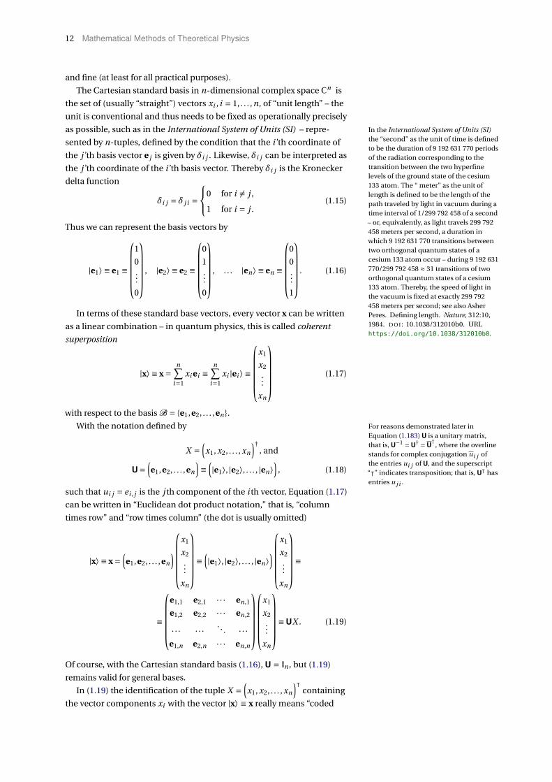
The Cartesian standard basis in n-dimensional complex space Cn is

the set of (usually “straight”) vectors xi , i = 1, . . . ,n, of “unit length” – the

unit is conventional and thus needs to be fixed as operationally precisely

as possible, such as in the International System of Units (SI) – repre- In the International System of Units (SI)the “second” as the unit of time is definedto be the duration of 9 192 631 770 periodsof the radiation corresponding to thetransition between the two hyperfinelevels of the ground state of the cesium133 atom. The “ meter” as the unit oflength is defined to be the length of thepath traveled by light in vacuum during atime interval of 1/299 792 458 of a second– or, equivalently, as light travels 299 792458 meters per second, a duration inwhich 9 192 631 770 transitions betweentwo orthogonal quantum states of acesium 133 atom occur – during 9 192 631770/299 792 458 ≈ 31 transitions of twoorthogonal quantum states of a cesium133 atom. Thereby, the speed of light inthe vacuum is fixed at exactly 299 792458 meters per second; see also AsherPeres. Defining length. Nature, 312:10,1984. D O I : 10.1038/312010b0. URLhttps://doi.org/10.1038/312010b0.

sented by n-tuples, defined by the condition that the i ’th coordinate of

the j ’th basis vector e j is given by δi j . Likewise, δi j can be interpreted as

the j ’th coordinate of the i ’th basis vector. Thereby δi j is the Kronecker

delta function

δi j = δ j i =0 for i 6= j ,

1 for i = j .(1.15)

Thus we can represent the basis vectors by

|e1⟩ ≡ e1 ≡

1

0...

0

, |e2⟩ ≡ e2 ≡

0

1...

0

, . . . |en⟩ ≡ en ≡

0

0...

1

. (1.16)

In terms of these standard base vectors, every vector x can be written

as a linear combination – in quantum physics, this is called coherent

superposition

|x⟩ ≡ x =n∑

i=1xi ei ≡

n∑i=1

xi |ei ⟩ ≡

x1

x2...

xn

(1.17)

with respect to the basis B = e1,e2, . . . ,en.

With the notation defined by For reasons demonstrated later inEquation (1.183) U is a unitary matrix,that is, U−1 = U† = U

ᵀ, where the overline

stands for complex conjugation ui j ofthe entries ui j of U, and the superscript“ᵀ” indicates transposition; that is, Uᵀ hasentries u j i .

X =(x1, x2, . . . , xn

)†, and

U=(e1,e2, . . . ,en

)≡

(|e1⟩, |e2⟩, . . . , |en⟩

), (1.18)

such that ui j = ei , j is the j th component of the i th vector, Equation (1.17)

can be written in “Euclidean dot product notation,” that is, “column

times row” and “row times column” (the dot is usually omitted)

|x⟩ ≡ x =(e1,e2, . . . ,en

)

x1

x2...

xn

≡(|e1⟩, |e2⟩, . . . , |en⟩

)

x1

x2...

xn

≡

≡

e1,1 e2,1 · · · en,1

e1,2 e2,2 · · · en,2

· · · · · · . . . · · ·e1,n e2,n · · · en,n

x1

x2...

xn

≡UX . (1.19)

Of course, with the Cartesian standard basis (1.16), U = In , but (1.19)

remains valid for general bases.

In (1.19) the identification of the tuple X =(x1, x2, . . . , xn

)ᵀcontaining

the vector components xi with the vector |x⟩ ≡ x really means “coded

Finite-dimensional vector spaces and linear algebra 13

with respect, or relative, to the basis B = e1,e2, . . . ,en.” Thus in what

follows, we shall often identify the column vector(x1, x2, . . . , xn

)ᵀcontain-

ing the coordinates of the vector with the vector x ≡ |x⟩, but we always

need to keep in mind that the tuples of coordinates are defined only with

respect to a particular basis e1,e2, . . . ,en; otherwise these numbers lack

any meaning whatsoever.

Indeed, with respect to some arbitrary basis B = f1, . . . , fn of some

n-dimensional vector space V with the base vectors fi , 1 ≤ i ≤ n, every

vector x in V can be written as a unique linear combination

|x⟩ ≡ x =n∑

i=1xi fi ≡

n∑i=1

xi |fi ⟩ ≡

x1

x2...

xn

(1.20)

with respect to the basis B = f1, . . . , fn.

The uniqueness of the coordinates is proven indirectly by reductio

ad absurdum: Suppose there is another decomposition x = ∑ni=1 yi fi =

(y1, y2, . . . , yn); then by subtraction, 0 =∑ni=1(xi − yi )fi = (0,0, . . . ,0). Since

the basis vectors fi are linearly independent, this can only be valid if all

coefficients in the summation vanish; thus xi − yi = 0 for all 1 ≤ i ≤ n;

hence finally xi = yi for all 1 ≤ i ≤ n. This is in contradiction with our

assumption that the coordinates xi and yi (or at least some of them) are

different. Hence the only consistent alternative is the assumption that,

with respect to a given basis, the coordinates are uniquely determined.

A set B = a1, . . . ,an of vectors of the inner product space V is or-

thonormal if, for all ai ∈B and a j ∈B, it follows that

⟨ai | a j ⟩ = δi j . (1.21)

Any such set is called complete if it is not a subset of any larger orthonor-

mal set of vectors of V . Any complete set is a basis. If, instead of Equa-

tion (1.21), ⟨ai | a j ⟩ = αiδi j with nonzero factors αi , the set is called

orthogonal.

1.7 Finding orthogonal bases from nonorthogonal ones

A Gram-Schmidt process10 is a systematic method for orthonormalising a 10 Steven J. Leon, Åke Björck, and WalterGander. Gram-Schmidt orthogonal-ization: 100 years and more. Numer-ical Linear Algebra with Applications,20(3):492–532, 2013. ISSN 1070-5325. D O I : 10.1002/nla.1839. URLhttps://doi.org/10.1002/nla.1839

set of vectors in a space equipped with a scalar product, or by a synonym

preferred in mathematics, inner product.

The Gram-Schmidt process takes a finite, linearly independent set of

base vectors and generates an orthonormal basis that spans the same

(sub)space as the original set.

The general method is to start out with the original basis, say,

14 Mathematical Methods of Theoretical Physics

x1,x2,x3, . . . ,xn, and generate a new orthogonal basis by

y1 = x1,

y2 = x2 −Py1 (x2),

y3 = x3 −Py1 (x3)−Py2 (x3),

...

yn = xn −n−1∑i=1

Pyi (xn), (1.22)

where y1,y2,y3, . . . ,yn The scalar or inner product ⟨x|y⟩ oftwo vectors x and y is defined on page7. In Euclidean space such as Rn , oneoften identifies the “dot product” x ·y =x1 y1 + ·· ·+ xn yn of two vectors x and ywith their scalar or inner product.

Py(x) = ⟨x|y⟩⟨y|y⟩y, and P⊥

y (x) = x− ⟨x|y⟩⟨y|y⟩y (1.23)

are the orthogonal projections of x onto y and y⊥, respectively (the latter

is mentioned for the sake of completeness and is not required here).

Note that these orthogonal projections are idempotent and mutually

orthogonal; that is,

P 2y (x) = Py(Py(x)) = ⟨x|y⟩

⟨y|y⟩⟨y|y⟩⟨y|y⟩y = Py(x),

(P⊥y )2(x) = P⊥

y (P⊥y (x)) = x− ⟨x|y⟩

⟨y|y⟩y−( ⟨x|y⟩⟨y|y⟩ −

⟨x|y⟩⟨y|y⟩⟨y|y⟩2

)y = P⊥

y (x),

Py(P⊥y (x)) = P⊥

y (Py(x)) = ⟨x|y⟩⟨y|y⟩y− ⟨x|y⟩⟨y|y⟩

⟨y|y⟩2 y = 0. (1.24)

For a more general discussion of projections, see also page 51.

Subsequently, in order to obtain an orthonormal basis, one can divide

every basis vector by its length.

The idea of the proof is as follows (see also Section 7.9 of Ref.11). In 11 Werner Greub. Linear Algebra, volume 23of Graduate Texts in Mathematics. Springer,New York, Heidelberg, fourth edition,1975

order to generate an orthogonal basis from a nonorthogonal one, the first

vector of the old basis is identified with the first vector of the new basis;

that is y1 = x1. Then, as depicted in Figure 1.2, the second vector of the

new basis is obtained by taking the second vector of the old basis and

subtracting its projection on the first vector of the new basis.

x1 = y1

x2

Py1 (x2)

y2 = x2 −Py1 (x2)

Figure 1.2: Gram-Schmidt constructionfor two nonorthogonal vectors x1 and x2,yielding two orthogonal vectors y1 and y2.

More precisely, take the Ansatz

y2 = x2 +λy1, (1.25)

thereby determining the arbitrary scalar λ such that y1 and y2 are orthog-

onal; that is, ⟨y2|y1⟩ = 0. This yields

⟨y1|y2⟩ = ⟨y1|x2⟩+λ⟨y1|y1⟩ = 0, (1.26)

and thus, since y1 6= 0,

λ=−⟨y1|x2⟩⟨y1|y1⟩

. (1.27)

To obtain the third vector y3 of the new basis, take the Ansatz

y3 = x3 +µy1 +νy2, (1.28)

and require that it is orthogonal to the two previous orthogonal basis

vectors y1 and y2; that is ⟨y1|y3⟩ = ⟨y2|y3⟩ = 0. We already know that

Finite-dimensional vector spaces and linear algebra 15

⟨y1|y2⟩ = 0. Consider the scalar products of y1 and y2 with the Ansatz for

y3 in Equation (1.28); that is,

⟨y1|y3⟩ = ⟨y1|x3⟩+µ⟨y1|y1⟩+ν⟨y1|y2⟩︸ ︷︷ ︸=0

= 0, (1.29)

and

⟨y2|y3⟩ = ⟨y2|x3⟩+µ⟨y2|y1⟩︸ ︷︷ ︸=0

+ν⟨y2|y2⟩ = 0. (1.30)

As a result,

µ=−⟨y1|x3⟩⟨y1|y1⟩

, ν=−⟨y2|x3⟩⟨y2|y2⟩

. (1.31)

A generalization of this construction for all the other new base vectors

y3, . . . ,yn , and thus a proof by complete induction, proceeds by a general-

ized construction.

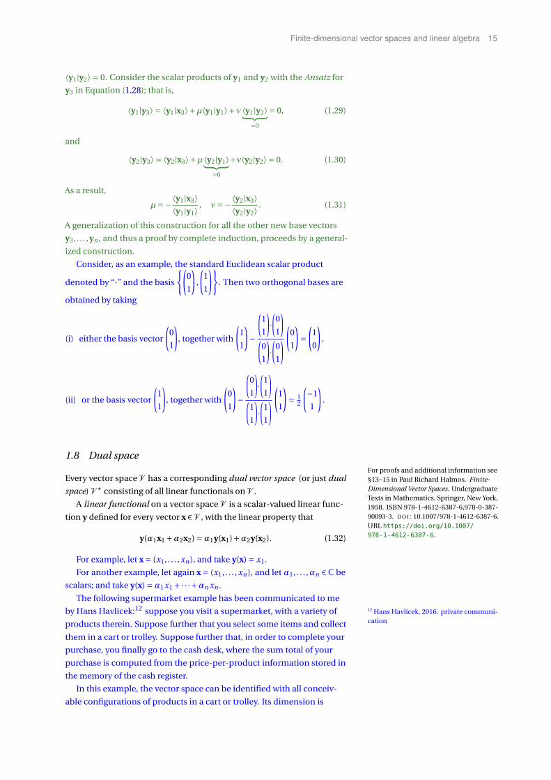
Consider, as an example, the standard Euclidean scalar product

denoted by “·” and the basis

(0

1

),

(1

1

). Then two orthogonal bases are

obtained by taking

(i) either the basis vector

(0

1

), together with

(1

1

)−

1

1

·0

1

0

1

·0

1

(

0

1

)=

(1

0

),

(ii) or the basis vector

(1

1

), together with

(0

1

)−

0

1

·1

1

1

1

·1

1

(

1

1

)= 1

2

(−1

1

).

1.8 Dual spaceFor proofs and additional information see§13–15 in Paul Richard Halmos. Finite-Dimensional Vector Spaces. UndergraduateTexts in Mathematics. Springer, New York,1958. ISBN 978-1-4612-6387-6,978-0-387-90093-3. D O I : 10.1007/978-1-4612-6387-6.URL https://doi.org/10.1007/

978-1-4612-6387-6.

Every vector space V has a corresponding dual vector space (or just dual

space) V ∗ consisting of all linear functionals on V .

A linear functional on a vector space V is a scalar-valued linear func-

tion y defined for every vector x ∈ V , with the linear property that

y(α1x1 +α2x2) =α1y(x1)+α2y(x2). (1.32)

For example, let x = (x1, . . . , xn), and take y(x) = x1.

For another example, let again x = (x1, . . . , xn), and let α1, . . . ,αn ∈C be

scalars; and take y(x) =α1x1 +·· ·+αn xn .

The following supermarket example has been communicated to me

by Hans Havlicek:12 suppose you visit a supermarket, with a variety of 12 Hans Havlicek, 2016. private communi-cationproducts therein. Suppose further that you select some items and collect

them in a cart or trolley. Suppose further that, in order to complete your

purchase, you finally go to the cash desk, where the sum total of your

purchase is computed from the price-per-product information stored in

the memory of the cash register.

In this example, the vector space can be identified with all conceiv-

able configurations of products in a cart or trolley. Its dimension is

16 Mathematical Methods of Theoretical Physics

determined by the number of different, mutually distinct products in

the supermarket. Its “base vectors” can be identified with the mutually

distinct products in the supermarket. The respective functional is the

computation of the price of any such purchase. It is based on a particular

price information. Every such price information contains one price per

item for all mutually distinct products. The dual space consists of all

conceivable price details.

We adopt a doublesquare bracket notation “J·, ·K” for the functional

y(x) = Jx,yK. (1.33)

Note that the usual arithmetic operations of addition and multiplica-

tion, that is,

(ay+bz)(x) = ay(x)+bz(x), (1.34)

together with the “zero functional” (mapping every argument to zero)

induce a kind of linear vector space, the “vectors” being identified with

the linear functionals. This vector space will be called dual space V ∗.

As a result, this “bracket” functional is bilinear in its two arguments;

that is,

Jα1x1 +α2x2,yK=α1Jx1,yK+α2Jx2,yK, (1.35)

and

Jx,α1y1 +α2y2K=α1Jx,y1K+α2Jx,y2K. (1.36)

The square bracket can be identified withthe scalar dot product Jx,yK= ⟨x | y⟩ onlyfor Euclidean vector spaces Rn , since forcomplex spaces this would no longer bepositive definite. That is, for Euclideanvector spaces Rn the inner or scalarproduct is bilinear.

Because of linearity, we can completely characterize an arbitrary

linear functional y ∈ V ∗ by its values of the vectors of some basis of V :

If we know the functional value on the basis vectors in B, we know the

functional on all elements of the vector space V . If V is an n-dimensional

vector space, and if B = f1, . . . , fn is a basis of V , and if α1, . . . ,αn is any

set of n scalars, then there is a unique linear functional y on V such that

Jfi ,yK=αi for all 0 ≤ i ≤ n.

A constructive proof of this theorem can be given as follows: Because

every x ∈ V can be written as a linear combination x = x1f1 +·· ·+ xn fn of

the basis vectors of B = f1, . . . , fn in one and only one (unique) way, we

obtain for any arbitrary linear functional y ∈ V ∗ a unique decomposition

in terms of the basis vectors of B = f1, . . . , fn; that is,

Jx,yK= x1Jf1,yK+·· ·+xnJfn ,yK. (1.37)

By identifying Jfi ,yK=αi we obtain

Jx,yK= x1α1 +·· ·+xnαn . (1.38)

Conversely, if we define y by Jx,yK = α1x1 + ·· ·+αn xn , then y can be

interpreted as a linear functional in V ∗ with Jfi ,yK=αi .

If we introduce a dual basis by requiring that Jfi , f∗j K = δi j (cf. Equa-

tion 1.39), then the coefficients Jfi ,yK=αi , 1 ≤ i ≤ n, can be interpreted

as the coordinates of the linear functional y with respect to the dual basis

B∗, such that y = (α1,α2, . . . ,αn)ᵀ.

Finite-dimensional vector spaces and linear algebra 17

Likewise, as will be shown in (1.46), xi = Jx, f∗i K; that is, the vector

coordinates can be represented by the functionals of the elements of the

dual basis.

Let us explicitly construct an example of a linear functional ϕ(x) ≡Jx,ϕK that is defined on all vectors x = αe1 +βe2 of a two-dimensional

vector space with the basis e1,e2 by enumerating its “performance on

the basis vectors” e1 =(1,0

)ᵀand e2 =

(0,1

)ᵀ; more explicitly, say, for an

example’s sake, ϕ(e1) ≡ Je1,ϕK = 2 and ϕ(e2) ≡ Je2,ϕK = 3. Therefore,

for example for the vector(5,7

)ᵀ, ϕ

((5,7

)ᵀ) ≡ r(5,7

)ᵀ,ϕ

z= 5Je1,ϕK+

7Je2,ϕK= 10+21 = 31.

In general the performance of the linear function on just one vector

renders insufficient information to uniquely define a linear functional

of vectors of dimension two or higher: one needs as many values on

mutually linear independent vectors as there are dimensions for a

complete specification of the linear functional. Take, for example, just

one value of ϕ on a single vector, say x =(5,7

)ᵀ; that is, ϕ (x) = 31. If

one does not know the linear functional beforehand, all one can do is

to write ϕ in terms of its components (with respect to the dual basis)

ϕ =(ϕ1,ϕ2

)and evaluate

(ϕ1,ϕ2

)·(5,7

)ᵀ = 5ϕ1 +7ϕ2 = 31, which just

yields one component of ϕ in terms of the other; that is, ϕ1 = (31−7ϕ2)/5.

The components of ϕ (with respect to the dual basis) are uniquely fixed

only by presentation of another value, say ϕ(y) = 13, on another vector

y =(2,3

)ᵀnot collinear to the first vector x. Then

(ϕ1,ϕ2

)·(2,3

)ᵀ =2ϕ1 +3ϕ2 = 13 yields ϕ1 = (13−3ϕ2)/2. Equating those two equations for

ϕ1 yields (31−7ϕ2)/5 = (13−3ϕ2)/2 and thus ϕ2 = 3 and therefore ϕ1 = 2.

1.8.1 Dual basis

We now can define a dual basis, or, used synonymously, a reciprocal or

contravariant basis. If V is an n-dimensional vector space, and if B =f1, . . . , fn is a basis of V , then there is a unique dual basis B∗ = f∗1 , . . . , f∗n

in the dual vector space V ∗ defined by

f∗j (fi ) = Jfi , f∗j K= δi j , (1.39)

where δi j is the Kronecker delta function. The dual space V ∗ spanned by

the dual basis B∗ is n-dimensional.

In a different notation involving subscripts (lower indices) for (basis)

vectors of the base vector space, and superscripts (upper indices) f j = f∗j ,

for (basis) vectors of the dual vector space, Equation (1.39) can be written

as

f j (fi ) = Jfi , f j K= δi j . (1.40)

Suppose g is a metric, facilitating the translation from vectors of the base

vectors into vectors of the dual space and vice versa (cf. Section 2.7.1 on

page 92 for a definition and more details), in particular, fi = gi l fl as well

as f∗j = f j = g j k fk . Then Eqs. (1.39) and (1.40) can be rewritten as

Jgi l fl , f j K= Jfi , g j k fkK= δi j . (1.41)

Note that the vectors f∗i = fi of the dual basis can be used to “retrieve”

18 Mathematical Methods of Theoretical Physics

the components of arbitrary vectors x =∑j x j f j through

f∗i (x) = f∗i

(∑j

x j f j

)=∑

jx j f∗i

(f j

)=∑j

x jδi j = xi . (1.42)

Likewise, the basis vectors fi can be used to obtain the coordinates of any

dual vector.

In terms of the inner products of the base vector space and its dual

vector space the representation of the metric may be defined by gi j =g (fi , f j ) = ⟨fi | f j ⟩, as well as g i j = g (fi , f j ) = ⟨fi | f j ⟩, respectively. Note,

however, that the coordinates gi j of the metric g need not necessarily

be positive definite. For example, special relativity uses the “pseudo-

Euclidean” metric g = diag(+1,+1,+1,−1) (or just g = diag(+,+,+,−)),

where “diag” stands for the diagonal matrix with the arguments in the

diagonal. The metric tensor gi j represents a

bilinear functional g (x,y) = xi y j gi jthat is symmetric; that is, g (x,y) = g (y,x)and nondegenerate; that is, for anynonzero vector x ∈ V , x 6= 0, there issome vector y ∈ V , so that g (x,y) 6= 0.g also satisfies the triangle inequality||x−z|| ≤ ||x−y||+ ||y−z||.

In a real Euclidean vector space Rn with the dot product as the scalar

product, the dual basis of an orthogonal basis is also orthogonal, and

contains vectors with the same directions, although with reciprocal

length (thereby explaining the wording “reciprocal basis”). Moreover,

for an orthonormal basis, the basis vectors are uniquely identifiable by

ei −→ e∗i = eᵀi . This identification can only be made for orthonormal

bases; it is not true for nonorthonormal bases.

A “reverse construction” of the elements f∗j of the dual basis B∗ –

thereby using the definition “Jfi ,yK=αi for all 1 ≤ i ≤ n” for any element

y in V ∗ introduced earlier – can be given as follows: for every 1 ≤ j ≤n, we can define a vector f∗j in the dual basis B∗ by the requirement

Jfi , f∗j K = δi j . That is, in words: the dual basis element, when applied to

the elements of the original n-dimensional basis, yields one if and only if

it corresponds to the respective equally indexed basis element; for all the

other n −1 basis elements it yields zero.

What remains to be proven is the conjecture that B∗ = f∗1 , . . . , f∗n is

a basis of V ∗; that is, that the vectors in B∗ are linear independent, and

that they span V ∗.

First observe that B∗ is a set of linear independent vectors, for if

α1f∗1 +·· ·+αn f∗n = 0, then also

Jx,α1f∗1 +·· ·+αn f∗nK=α1Jx, f∗1 K+·· ·+αnJx, f∗nK= 0 (1.43)

for arbitrary x ∈ V . In particular, by identifying x with fi ∈B, for 1 ≤ i ≤ n,

α1Jfi , f∗1 K+·· ·+αnJfi , f∗nK=α j Jfi , f∗j K=α jδi j =αi = 0. (1.44)

Second, every y ∈ V ∗ is a linear combination of elements in B∗ =f∗1 , . . . , f∗n, because by starting from Jfi ,yK= αi , with x = x1f1 +·· ·+ xn fn

we obtain

Jx,yK= x1Jf1,yK+·· ·+xnJfn ,yK= x1α1 +·· ·+xnαn . (1.45)

Note that , for arbitrary x ∈ V ,

Jx, f∗i K= x1Jf1, f∗i K+·· ·+xnJfn , f∗i K= x j Jf j , f∗i K= x jδ j i = xi , (1.46)

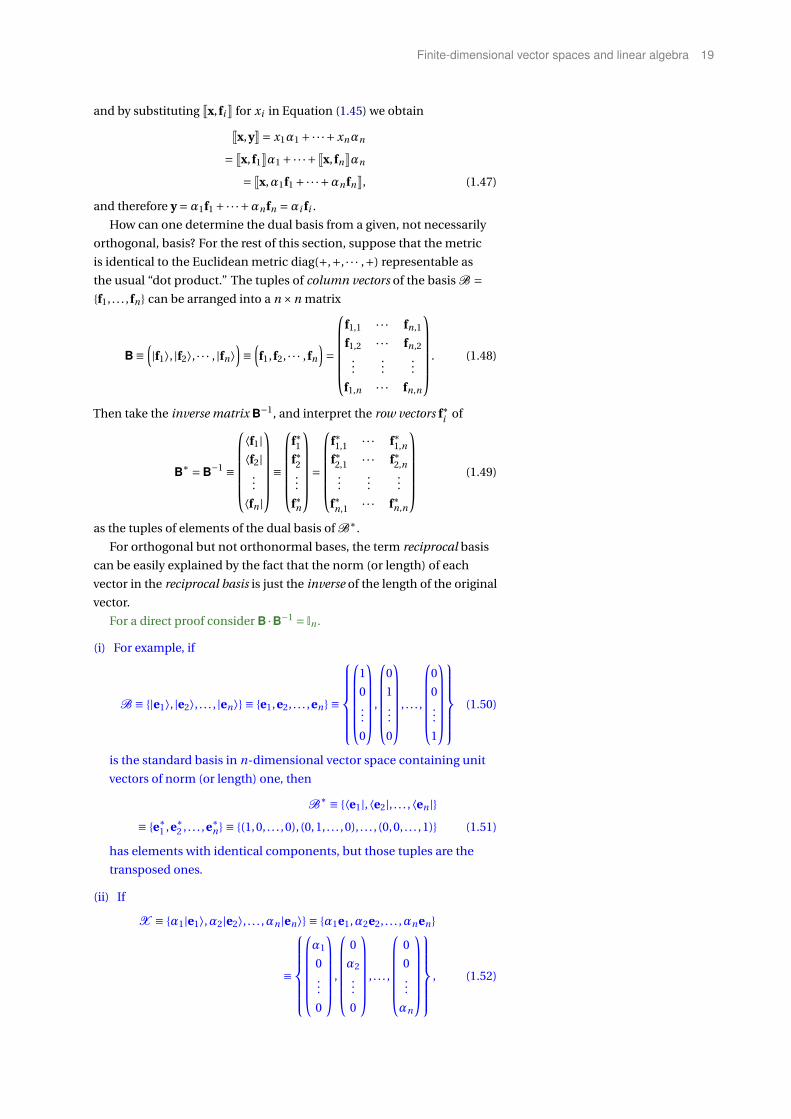
Finite-dimensional vector spaces and linear algebra 19

and by substituting Jx, fi K for xi in Equation (1.45) we obtain

Jx,yK= x1α1 +·· ·+xnαn

= Jx, f1Kα1 +·· ·+ Jx, fnKαn

= Jx,α1f1 +·· ·+αn fnK, (1.47)

and therefore y =α1f1 +·· ·+αn fn =αi fi .

How can one determine the dual basis from a given, not necessarily

orthogonal, basis? For the rest of this section, suppose that the metric

is identical to the Euclidean metric diag(+,+, · · · ,+) representable as

the usual “dot product.” The tuples of column vectors of the basis B =f1, . . . , fn can be arranged into a n ×n matrix

B≡(|f1⟩, |f2⟩, · · · , |fn⟩

)≡

(f1, f2, · · · , fn

)=

f1,1 · · · fn,1

f1,2 · · · fn,2...

......

f1,n · · · fn,n

. (1.48)

Then take the inverse matrix B−1, and interpret the row vectors f∗i of

B∗ =B−1 ≡

⟨f1|⟨f2|

...

⟨fn |

≡

f∗1f∗2...

f∗n

=

f∗1,1 · · · f∗1,n

f∗2,1 · · · f∗2,n...

......

f∗n,1 · · · f∗n,n

(1.49)

as the tuples of elements of the dual basis of B∗.

For orthogonal but not orthonormal bases, the term reciprocal basis

can be easily explained by the fact that the norm (or length) of each

vector in the reciprocal basis is just the inverse of the length of the original

vector.

For a direct proof consider B ·B−1 = In .

(i) For example, if

B ≡ |e1⟩, |e2⟩, . . . , |en⟩ ≡ e1,e2, . . . ,en ≡

1

0...

0

,

0

1...

0

, . . . ,

0

0...

1

(1.50)

is the standard basis in n-dimensional vector space containing unit

vectors of norm (or length) one, then

B∗ ≡ ⟨e1|,⟨e2|, . . . ,⟨en |≡ e∗1 ,e∗2 , . . . ,e∗n ≡ (1,0, . . . ,0), (0,1, . . . ,0), . . . , (0,0, . . . ,1) (1.51)

has elements with identical components, but those tuples are the

transposed ones.

(ii) If

X ≡ α1|e1⟩,α2|e2⟩, . . . ,αn |en⟩ ≡ α1e1,α2e2, . . . ,αn en

≡

α1

0...

0

,

0

α2...

0

, . . . ,

0

0...

αn

, (1.52)

20 Mathematical Methods of Theoretical Physics

with nonzero α1,α2, . . . ,αn ∈ R, is a “dilated” basis in n-dimensional

vector space containing vectors of norm (or length) αi , then

X ∗ ≡

1

α1⟨e1|, 1

α2⟨e2|, . . . ,

1

αn⟨en |

≡

1

α1e∗1 ,

1

α2e∗2 , . . . ,

1

αne∗n

≡

(1α1

,0, . . . ,0)

,(0, 1

α2, . . . ,0

), . . . ,

(0,0, . . . , 1

αn

)(1.53)

has elements with identical components of inverse length 1αi

, and

again those tuples are the transposed tuples.

(iii) Consider the nonorthogonal basis B =(

1

3

),

(2

4

). The associated

column matrix is

B=(

1 2

3 4

). (1.54)

The inverse matrix is

B−1 =(−2 1

32 − 1

2

), (1.55)

and the associated dual basis is obtained from the rows of B−1 by

B∗ =(−2,1

),(

32 ,− 1

2

)= 1

2

(−4,2

),(3,−1

). (1.56)

1.8.2 Dual coordinates

With respect to a given basis, the components of a vector are often

written as tuples of ordered (“xi is written before xi+1” – not “xi < xi+1”)

scalars as column vectors

|x⟩ ≡ x ≡(x1, x2, · · · , xn

)ᵀ, (1.57)

whereas the components of vectors in dual spaces are often written in

terms of tuples of ordered scalars as row vectors

⟨x| ≡ x∗ ≡(x∗

1 , x∗2 , . . . , x∗

n

). (1.58)

The coordinates of vectors |x⟩ ≡ x of the base vector space V – and by

definition (or rather, declaration) the vectors |x⟩ ≡ x themselves – are

called contravariant: because in order to compensate for scale changes

of the reference axes (the basis vectors) |e1⟩, |e2⟩, . . . , |en⟩ ≡ e1,e2, . . . ,en

these coordinates have to contra-vary (inversely vary) with respect to any

such change.

In contradistinction the coordinates of dual vectors, that is, vectors of

the dual vector space V ∗, ⟨x| ≡ x∗ – and by definition (or rather, declara-

tion) the vectors ⟨x| ≡ x∗ themselves – are called covariant.

Alternatively covariant coordinates could be denoted by subscripts

(lower indices), and contravariant coordinates can be denoted by su-

perscripts (upper indices); that is (see also Havlicek13, Section 11.4), 13 Hans Havlicek. Lineare Algebra fürTechnische Mathematiker. HeldermannVerlag, Lemgo, second edition, 2008

x ≡ |x⟩ ≡(x1, x2, · · · , xn

)ᵀ, and

x∗ ≡ ⟨x| ≡ (x∗1 , x∗

2 , . . . , x∗n ) ≡ (x1, x2, . . . , xn). (1.59)

Finite-dimensional vector spaces and linear algebra 21

This notation will be used in the chapter 2 on tensors. Note again that the

covariant and contravariant components xk and xk are not absolute, but

always defined with respect to a particular (dual) basis.

Note that, for orthormal bases it is possible to interchange contravari-

ant and covariant coordinates by taking the conjugate transpose; that is,

(⟨x|)† = |x⟩, and (|x⟩)† = ⟨x|. (1.60)

Note also that the Einstein summation convention requires that, when

an index variable appears twice in a single term, one has to sum over all

of the possible index values. This saves us from drawing the sum sign

“∑

i ” for the index i ; for instance xi yi =∑i xi yi .

In the particular context of covariant and contravariant components

– made necessary by nonorthogonal bases whose associated dual bases

are not identical – the summation always is between some superscript

(upper index) and some subscript (lower index); e.g., xi y i .

Note again that for orthonormal basis, xi = xi .

1.8.3 Representation of a functional by inner productFor proofs and additional informationsee §67 in Paul Richard Halmos. Finite-Dimensional Vector Spaces. UndergraduateTexts in Mathematics. Springer, New York,1958. ISBN 978-1-4612-6387-6,978-0-387-90093-3. D O I : 10.1007/978-1-4612-6387-6.URL https://doi.org/10.1007/

978-1-4612-6387-6.

The following representation theorem, often called Riesz representation

theorem (sometimes also called the Fréchet-Riesz theorem), is about

the connection between any functional in a vector space and its inner

product: To any linear functional z on a finite-dimensional inner product

space V there corresponds a unique vector y ∈ V , such that

z(x) ≡ Jx,zK= ⟨y | x⟩ (1.61)

for all x ∈ V . See Theorem 4.12 in Walter Rudin.Real and complex analysis. McGraw-Hill, New York, third edition, 1986.ISBN 0-07-100276-6. URL https:

//archive.org/details/RudinW.

RealAndComplexAnalysis3e1987/page/

n0.

A constructive proof provides a method to compute the vector y ∈ V

given the linear functional z ∈ V ∗. The proof idea is to “go back” to the

target vector y from the original vector z by formation of the “orthogonal”

subspace twice – the first time defining a kind of “orthogonality” between

a functional z ∈ V ∗ and vectors z ∈ V by z(x) = 0.

Let us first consider the case of z = 0, for which we can ad hoc identify

the zero vector with y; that is, y = 0.

For any nonzero z(x) 6= 0 on some x we first need to locate the sub-

space

M =

x∣∣∣z(x) = 0,x ∈ V

(1.62)

consisting of all vectors x for which z(x) vanishes.

In a second step consider M⊥, the orthogonal complement of M with

respect to V . M⊥ consists of all vectors orthogonal to all vectors in M ,

such that ⟨x | w⟩ = 0 for x ∈M and w ∈M⊥.

The assumption z(x) 6= 0 on some x guarantees that M⊥ does not

consist of the zero vector 0 alone. That is, M⊥ must contain a nonzero

unit vector y0 ∈ M⊥. (It turns out that M⊥ is one-dimensional and

spanned by y0; that is, up to a multiplicative constant y0 is proportional

to the vector y.)

In a next step define the vector

u = z(x)y0 −z(y0)x (1.63)

22 Mathematical Methods of Theoretical Physics

for which, due to linearity of z,

z(u) = z[

z(x)y0 −z(y0)x]= z(x)z(y0)−z(y0)z(x) = 0. (1.64)

Thus u ∈M , and therefore also ⟨u | y0⟩ = 0. Insertion of u from (1.63) and

antilinearity in the first argument and linearity in the second argument of

the inner product yields

⟨z(x)y0 −z(y0)x | y0⟩ = 0,

z(x)⟨y0 | y0⟩︸ ︷︷ ︸=1

−z(y0)⟨x | y0⟩ = 0,

z(x) = z(y0)⟨y0 | x⟩ = ⟨z(y0)y0 | x⟩. (1.65)

Thus we can identify the “target” vector

y = z(y0)y0 (1.66)

associated with the functional z.

The proof of uniqueness is by (wrongly) assuming that there exist two

(presumably different) y1 and y2 such that ⟨x|y1⟩ = ⟨x|y2⟩ for all x ∈ V .

Due to linearity of the scalar product, ⟨x|y1 −y2⟩ = 0; in particular, if we

identify x = y1 −y2, then ⟨y1 −y2|y1 −y2⟩ = 0 and thus y1 = y2.

This proof is constructive in the sense that it yields y, given z. Note

that, because of uniqueness, M⊥ has to be a one dimensional subspace

of V spanned by the unit vector y0.

Another, more direct, proof is a straightforward construction of the

“target” vector y ∈ V associated with the linear functional z ∈ V ∗ in terms

of some orthonormal basis B = e1, . . . ,en of V : We obtain the compo-

nents (coordinates) yi , 1 ≤ i ≤ n of y = ∑nj=1 y j e j ≡

(y1, · · · , yn

)ᵀwith

respect to the orthonormal basis (coordinate system) B by evaluating the

“performance” of z on all vectors of the basis ei , 1 ≤ i ≤ n in that basis:

z(ei ) = ⟨y | ei ⟩ =⟨ n∑

j=1y j e j

∣∣ei⟩= n∑

j=1y j ⟨e j | ei︸ ︷︷ ︸

δi j

⟩ = yi . (1.67)

Hence, the “target” vector can be written as

y =n∑

j=1z(e j )e j . (1.68)

Both proofs yield the same “target” vector y associated with z, as inser-

tion into (1.66) and (1.67) results in Einstein’s summation convention is usedhere.

y = z(y0)y0 = z

(yi√⟨y | y⟩ei

)y j√⟨y | y⟩e j

= yi

⟨y | y⟩ z (ei )︸ ︷︷ ︸yi

y j e j = yi yi

⟨y | y⟩ y j e j = y j e j . (1.69)

In the Babylonian tradition14 and for the sake of an example consider

14 The Babylonians “proved” arithmeticalstatements by inserting “large numbers”in the respective conjectures; cf. ChapterV of Otto Neugebauer. Vorlesungen überdie Geschichte der antiken mathema-tischen Wissenschaften. 1. Band: Vor-griechische Mathematik. Springer, Berlin,Heidelberg, 1934. ISBN 978-3-642-95096-4,978-3-642-95095-7. D O I : 10.1007/978-3-642-95095-7. URL https://doi.org/10.

1007/978-3-642-95095-7

the Cartesian standard basis of V = R2; with the two basis vectors e1 =(1,0

)ᵀand e2 =

(0,1

)ᵀ. Suppose further that the linear functional z is

defined by its “behavior” on these basis elements e1 and e2 as follows:

z(e1) = 1, z(e2) = 2. (1.70)

Finite-dimensional vector spaces and linear algebra 23

In a first step, let us construct M = x | z(x) = 0,x ∈ R2. Consider an

arbitrary vector x = x1e1 +x2e2 ∈M . Then,

z(x) = z(x1e1 +x2e2) = x1z(e1)+x2z(e2) = x1 +2x2 = 0, (1.71)

and therefore x1 = −2x2. The normalized vector spanning M thus is1p5

(−2,1

)ᵀ.

In the second step, a normalized vector y0 ∈ N = M⊥ orthogonal

to M is constructed by 1p5

(−2,1

)ᵀ ·y0 = 0, resulting in y0 = 1p5

(1,2

)ᵀ =1p5

(e1 +2e2).

In the third and final step y is constructed through

y = z(y0)y0 = z(

1p5

(e1 +2e2)

)1p5

(1,2

)ᵀ= 1

5[z(e1)+2z(e2)]

(1,2

)ᵀ = 1

5[1+4]

(1,2

)ᵀ = (1,2

)ᵀ. (1.72)

It is always prudent – and in the “Babylonian spirit” – to check this out

by inserting “large numbers” (maybe even primes): suppose x =(11,13

)ᵀ;

then z(x) = 11+26 = 37; whereas, according to Equation (1.61), ⟨y | x⟩ =(1,2

)ᵀ · (11,13)ᵀ = 37.

Note that in real or complex vector space Rn or Cn , and with the dot

product, y† ≡ z. Indeed, this construction induces a “conjugate” (in the

complex case, referring to the conjugate symmetry of the scalar product

in Equation (1.61), which is conjugate-linear in its second argument)

isomorphisms between a vector space V and its dual space V ∗.

Note also that every inner product ⟨y | x⟩ = φy (x) defines a linear

functional φy (x) for all x ∈ V .

In quantum mechanics, this representation of a functional by the

inner product suggests the (unique) existence of the bra vector ⟨ψ| ∈ V ∗

associated with every ket vector |ψ⟩ ∈ V .

It also suggests a “natural” duality between propositions and states –

that is, between (i) dichotomic (yes/no, or 1/0) observables represented

by projections Ex = |x⟩⟨x| and their associated linear subspaces spanned

by unit vectors |x⟩ on the one hand, and (ii) pure states, which are also

represented by projections ρψ = |ψ⟩⟨ψ| and their associated subspaces

spanned by unit vectors |ψ⟩ on the other hand – via the scalar product

“⟨·|·⟩.” In particular,15 15 Jan Hamhalter. Quantum MeasureTheory. Fundamental Theories of Physics,Vol. 134. Kluwer Academic Publishers,Dordrecht, Boston, London, 2003. ISBN1-4020-1714-6

ψ(x) = ⟨ψ | x⟩ (1.73)

represents the probability amplitude. By the Born rule for pure states, the

absolute square |⟨x |ψ⟩|2 of this probability amplitude is identified with

the probability of the occurrence of the proposition Ex, given the state

|ψ⟩.More general, due to linearity and the spectral theorem (cf. Section

1.27.1 on page 63), the statistical expectation for a Hermitian (normal)

operator A=∑ki=0λi Ei and a quantized system prepared in pure state (cf.

Section 1.24) ρψ = |ψ⟩⟨ψ| for some unit vector |ψ⟩ is given by the Born

24 Mathematical Methods of Theoretical Physics

rule

⟨A⟩ψ = Tr(ρψA) = Tr

[ρψ

(k∑

i=0λi Ei

)]= Tr

(k∑

i=0λiρψEi

)

= Tr

(k∑

i=0λi (|ψ⟩⟨ψ|)(|xi ⟩⟨xi |)

)= Tr

(k∑

i=0λi |ψ⟩⟨ψ|xi ⟩⟨xi |

)

=k∑

j=0⟨x j |

(k∑

i=0λi |ψ⟩⟨ψ|xi ⟩⟨xi |

)|x j ⟩

=k∑

j=0

k∑i=0

λi ⟨x j |ψ⟩⟨ψ|xi ⟩⟨xi |x j ⟩︸ ︷︷ ︸δi j

=k∑

i=0λi ⟨xi |ψ⟩⟨ψ|xi ⟩ =

k∑i=0

λi |⟨xi |ψ⟩|2, (1.74)

where Tr stands for the trace (cf. Section 1.17 on page 40), and we have

used the spectral decomposition A=∑ki=0λi Ei (cf. Section 1.27.1 on page

63).

1.8.4 Double dual space

In the following, we strictly limit the discussion to finite dimensional

vector spaces.

Because to every vector space V there exists a dual vector space V ∗

“spanned” by all linear functionals on V , there exists also a dual vector

space (V ∗)∗ = V ∗∗ to the dual vector space V ∗ “spanned” by all linear

functionals on V ∗. This construction can be iterated and is the basis of a

constructively definable “succession” of spaces of ever increasing duality.

At the same time, by a sort of “inversion” of the linear functional (or

by exchanging the corresponding arguments of the inner product) every

vector in V can be thought of as a linear functional on V ∗: just define

x(y)def≡ y(x) for x ∈ V and y ∈ V ∗, thereby rendering an element in V ∗∗. So

is there some sort of “connection” between a vector space and its double

dual space? For proofs and additional informationsee §16 in Paul Richard Halmos. Finite-Dimensional Vector Spaces. UndergraduateTexts in Mathematics. Springer, New York,1958. ISBN 978-1-4612-6387-6,978-0-387-90093-3. D O I : 10.1007/978-1-4612-6387-6.URL https://doi.org/10.1007/

978-1-4612-6387-6.

We state without proof that indeed there is a canonical identification

between V and V ∗∗: corresponding to every linear functional z ∈ V ∗∗

on the dual space V ∗ of V there exists a vector x ∈ V such that z(y) = y(x)

for every y ∈ V ∗. Thereby this x−z correspondence V ≡ V ∗∗ between V

and V ∗∗ is an isomorphism; that is, a structure preserving map which is

one-to-one and onto.

With this in mind, we obtain

V ≡ V ∗∗,

V ∗ ≡ V ∗∗∗,

V ∗∗ ≡ V ∗∗∗∗ ≡ V ,

V ∗∗∗ ≡ V ∗∗∗∗∗ ≡ V ∗,

... (1.75)

Finite-dimensional vector spaces and linear algebra 25

1.9 Direct sumFor proofs and additional information see§18, §19 in Paul Richard Halmos. Finite-Dimensional Vector Spaces. UndergraduateTexts in Mathematics. Springer, New York,1958. ISBN 978-1-4612-6387-6,978-0-387-90093-3. D O I : 10.1007/978-1-4612-6387-6.URL https://doi.org/10.1007/

978-1-4612-6387-6.

Let U and V be vector spaces (over the same field, say C). Their direct

sum is a vector space W =U ⊕V consisting of all ordered pairs (x,y), with

x ∈U and y ∈ V , and with the linear operations defined by

(αx1 +βx2,αy1 +βy2) =α(x1,y1)+β(x2,y2). (1.76)

Note that, just like vector addition, addition is defined coordinate-

wise.

We state without proof that the dimension of the direct sum is the sum

of the dimensions of its summands.

We also state without proof that, if U and V are subspaces of a vector For proofs and additional informationsee §18 in Paul Richard Halmos. Finite-Dimensional Vector Spaces. UndergraduateTexts in Mathematics. Springer, New York,1958. ISBN 978-1-4612-6387-6,978-0-387-90093-3. D O I : 10.1007/978-1-4612-6387-6.URL https://doi.org/10.1007/

978-1-4612-6387-6.

space W , then the following three conditions are equivalent:

(i) W =U ⊕V ;

(ii) U⋂

V =O and U +V =W , that is, W is spanned by U and V (i.e., U

and V are complements of each other);

(iii) every vector z ∈W can be written as z = x+y, with x ∈U and y ∈ V , in

one and only one way.

Very often the direct sum will be used to “compose” a vector space

by the direct sum of its subspaces. Note that there is no “natural” way of

composition. A different way of putting two vector spaces together is by

the tensor product.

1.10 Tensor productFor proofs and additional informationsee §24 in Paul Richard Halmos. Finite-Dimensional Vector Spaces. UndergraduateTexts in Mathematics. Springer, New York,1958. ISBN 978-1-4612-6387-6,978-0-387-90093-3. D O I : 10.1007/978-1-4612-6387-6.URL https://doi.org/10.1007/

978-1-4612-6387-6.

1.10.1 Sloppy definition

For the moment, suffice it to say that the tensor product V ⊗U of two

linear vector spaces V and U should be such that, to every x ∈ V and

every y ∈U there corresponds a tensor product z = x⊗y ∈ V ⊗U which is

bilinear; that is, linear in both factors.

A generalization to more factors appears to present no further concep-

tual difficulties.

1.10.2 Definition

A more rigorous definition is as follows: The tensor product V ⊗U of

two vector spaces V and U (over the same field, say C) is the dual vector

space of all bilinear forms on V ⊕U .

For each pair of vectors x ∈ V and y ∈U the tensor product z = x⊗y is

the element of V ⊗U such that z(w) = w(x,y) for every bilinear form w on

V ⊕U .

Alternatively we could define the tensor product as the coherent

superpositions of products ei ⊗ f j of all basis vectors ei ∈ V , with 1 ≤ i ≤ n,

and f j ∈U , with 1 ≤ j ≤ m as follows. First we note without proof that if

A = e1, . . . ,en and B = f1, . . . , fm are bases of n- and m- dimensional

vector spaces V and U , respectively, then the set of vectors ei ⊗ f j with

i = 1, . . .n and j = 1, . . .m is a basis of the tensor product V ⊗U . Then an

26 Mathematical Methods of Theoretical Physics

arbitrary tensor product can be written as the coherent superposition

of all its basis vectors ei ⊗ f j with ei ∈ V , with 1 ≤ i ≤ n, and f j ∈U , with

1 ≤ j ≤ m; that is,

z =∑i , j

ci j ei ⊗ f j . (1.77)

We state without proof that the dimension of V ⊗ U of an n-

dimensional vector space V and an m-dimensional vector space U

is multiplicative, that is, the dimension of V ⊗U is nm. Informally, this is

evident from the number of basis pairs ei ⊗ f j .

1.10.3 Representation

A tensor (dyadic, outer) product z = x⊗y of two vectors x and y has three

equivalent notations or representations:

(i) as the scalar coordinates xi y j with respect to the basis in which the

vectors x and y have been defined and encoded;

(ii) as a quasi-matrix zi j = xi y j , whose components zi j are defined with

respect to the basis in which the vectors x and y have been defined

and encoded;

(iii) as a list, or quasi-vector, or “flattened matrix” defined by the Kro-

necker product z = (x1y, x2y, . . . , xn y)ᵀ = (x1 y1, x1 y2, . . . , xn yn)ᵀ. Again,

the scalar coordinates xi y j are defined with respect to the basis in

which the vectors x and y have been defined and encoded.

In all three cases, the pairs xi y j are properly represented by distinct

mathematical entities.

Take, for example, x = (2,3)ᵀ and y = (5,7,11)ᵀ. Then z = x⊗ y can

be represented by (i) the four scalars x1 y1 = 10, x1 y2 = 14, x1 y3 = 22,

x2 y1 = 15, x2 y2 = 21, x2 y3 = 33, or by (ii) a 2×3 matrix

(10 14 22

15 21 33

), or by

(iii) a 4-tuple(10,14,22,15,21,33

)ᵀ.

Note, however, that this kind of quasi-matrix or quasi-vector repre-

sentation of vector products can be misleading insofar as it (wrongly)

suggests that all vectors in the tensor product space are accessible (rep-

resentable) as quasi-vectors – they are, however, accessible by coherent

superpositions (1.77) of such quasi-vectors. For instance, take the ar- In quantum mechanics this amountsto the fact that not all pure two-particlestates can be written in terms of (ten-sor) products of single-particle states;see also Section 1.5 of David N. Mer-min. Quantum Computer Science.Cambridge University Press, Cam-bridge, 2007. ISBN 9780521876582.D O I : 10.1017/CBO9780511813870.URL https://doi.org/10.1017/

CBO9780511813870.

bitrary form of a (quasi-)vector in C4, which can be parameterized by

(α1,α2,α3,α4

)ᵀ, with α1,α3,α3,α4 ∈C, (1.78)

and compare (1.78) with the general form of a tensor product of two

quasi-vectors in C2

(a1, a2

)ᵀ⊗ (b1,b2

)ᵀ ≡ (a1b1, a1b2, a2b1, a2b2

)ᵀ, with a1, a2,b1,b2 ∈C.

(1.79)

A comparison of the coordinates in (1.78) and (1.79) yields

α1 = a1b1, α2 = a1b2, α3 = a2b1, α4 = a2b2. (1.80)

Finite-dimensional vector spaces and linear algebra 27

By taking the quotient of the two first and the two last equations, and by

equating these quotients, one obtains

α1

α2= b1

b2= α3

α4, and thus α1α4 =α2α3, (1.81)

which amounts to a condition for the four coordinates α1,α2,α3,α4 in

order for this four-dimensional vector to be decomposable into a tensor

product of two two-dimensional quasi-vectors. In quantum mechanics,

pure states which are not decomposable into a product of single-particle

states are called entangled.

A typical example of an entangled state is the Bell state, |Ψ−⟩ or, more

generally, states in the Bell basis : with the notation a⊗b ≡ ab ≡ |a⟩⊗ |b⟩ ≡|a⟩|b⟩ ≡ |ab⟩ and the identifications |0⟩ ≡

(1,0

)ᵀand |1⟩ ≡

(0,1

)ᵀ|Ψ±⟩ = 1p

2(|0⟩|1⟩± |1⟩|0⟩) ≡ 1p

2(|01⟩± |10⟩)

≡(1,0

)ᵀ (0,1

)ᵀ± (0,1

)ᵀ (1,0

)ᵀ = (0,1,±1,0

)ᵀ,

|Φ±⟩ = 1p2

(|0⟩|0⟩± |1⟩|1⟩) ≡ 1p2

(|00⟩± |11⟩)

≡(1,0

)ᵀ (1,0

)ᵀ± (0,1

)ᵀ (0,1

)ᵀ = (1,0,0,±1

)ᵀ. (1.82)

For instance, in the case of |Ψ−⟩ a comparison of coefficient yields

α1 = a1b1 = 0 = a2b2 =α4,

α2 = a1b2 = 1p2= a2b1 =α3; (1.83)

and thus the entanglement, since

α1α4 = 0 6=α2α3 = 1

2. (1.84)

This shows that |Ψ−⟩ cannot be considered as a two particle product

state. Indeed, the state can only be characterized by considering the

relative properties of the two particles – in the case of |Ψ−⟩ they are

associated with the statements:16 “the quantum numbers (in this case “0” 16 Anton Zeilinger. A foundational principlefor quantum mechanics. Foundationsof Physics, 29(4):631–643, 1999. D O I :10.1023/A:1018820410908. URL https:

//doi.org/10.1023/A:1018820410908

and “1”) of the two particles are always different.”

1.11 Linear transformationFor proofs and additional information see§32-34 in Paul Richard Halmos. Finite-Dimensional Vector Spaces. UndergraduateTexts in Mathematics. Springer, New York,1958. ISBN 978-1-4612-6387-6,978-0-387-90093-3. D O I : 10.1007/978-1-4612-6387-6.URL https://doi.org/10.1007/

978-1-4612-6387-6.

1.11.1 Definition

A linear transformation, or, used synonymously, a linear operator, A on

a vector space V is a correspondence that assigns every vector x ∈ V a

vector Ax ∈ V , in a linear way; such that

A(αx+βy) =αA(x)+βA(y) =αAx+βAy, (1.85)

identically for all vectors x,y ∈ V and all scalars α,β.

1.11.2 Operations

The sum S = A+B of two linear transformations A and B is defined by

Sx =Ax+Bx for every x ∈ V .

28 Mathematical Methods of Theoretical Physics

The product P = AB of two linear transformations A and B is defined

by Px =A(Bx) for every x ∈ V .

The notation AnAm = An+m and (An)m = Anm , with A1 = A and A0 = 1turns out to be useful.

With the exception of commutativity, all formal algebraic properties

of numerical addition and multiplication, are valid for transformations;

that is A0 = 0A = 0, A1 = 1A = A, A(B+C) = AB+AC, (A+B)C = AC+BC,

and A(BC) = (AB)C. In matrix notation, 1 = 1, and the entries of 0 are 0

everywhere.

The inverse operator A−1 of A is defined by AA−1 =A−1A= I.The commutator of two matrices A and B is defined by

[A,B] =AB−BA. (1.86)

The commutator should not be confusedwith the bilinear functional introduced fordual spaces.

In terms of this matrix notation, it is quite easy to present an example

for which the commutator [A,B] does not vanish; that is A and B do not

commute.

Take, for the sake of an example, the Pauli spin matrices which are

proportional to the angular momentum operators of spin- 12 particles

along the x, y , z-axis: For more general angular momentumoperators see Leonard I. Schiff. QuantumMechanics. McGraw-Hill, New York, 1955.

σ1 =σx =(

0 1

1 0

),

σ2 =σy =(

0 −i

i 0

),

σ3 =σz =(

1 0

0 −1

). (1.87)

Together with the identity, that is, with I2 = diag(1,1), they form a com-

plete basis of all (4×4) matrices. Now take, for instance, the commutator

[σ1,σ3] =σ1σ3 −σ3σ1

=(

0 1

1 0

)(1 0

0 −1

)−

(1 0

0 −1

)(0 1

1 0

)

= 2

(0 −1

1 0

)6=

(0 0

0 0

). (1.88)

The polynomial can be directly adopted from ordinary arithmetic; that

is, any finite polynomial p of degree n of an operator (transformation) Acan be written as

p(A) =α01+α1A1 +α2A2 +·· ·+αnAn =n∑

i=0αi Ai . (1.89)

The Baker-Hausdorff formula

e iABe−iA = B + i [A,B]+ i 2

2![A, [A,B]]+·· · (1.90)

for two arbitrary noncommutative linear operators A and B is mentioned

without proof17).

17 A. Messiah. Quantum Mechanics,volume I. North-Holland, Amsterdam,1962

Finite-dimensional vector spaces and linear algebra 29

If [A,B] commutes with A and B, then

eAeB = eA+B+ 12 [A,B]. (1.91)

If A commutes with B, then

eAeB = eA+B. (1.92)

1.11.3 Linear transformations as matrices

Let V be an n-dimensional vector space; let B = |f1⟩, |f2⟩, . . . , |fn⟩ be any

basis of V , and let A be a linear transformation on V .

Because every vector is a linear combination of the basis vectors |fi ⟩,every linear transformation can be defined by “its performance on the

basis vectors;” that is, by the particular mapping of all n basis vectors

into the transformed vectors, which in turn can be represented as linear

combination of the n basis vectors.

Therefore it is possible to define some n ×n matrix with n2 coefficients

or coordinates αi j such that

A|f j ⟩ =∑

iαi j |fi ⟩ (1.93)

for all j = 1, . . . ,n. Again, note that this definition of a transformation

matrix is “tied to” a basis.

The “reverse order” of indices in (1.93) has been chosen in order for

the vector coordinates to transform in the “right order:” with (1.17) on

page 12: note that

A|x⟩ =A∑

jx j |f j ⟩ =

∑j

Ax j |f j ⟩ =∑

jx j A|f j ⟩ =

∑i , j

x jαi j |fi ⟩

=∑i , jαi j x j |fi ⟩ = (i ↔ j ) =∑

j ,iα j i xi |f j ⟩, (1.94)

and thus, because A|x⟩ = [A|x⟩] j |f j ⟩,

∑j

([A|x⟩] j −

∑iα j i xi

)|f j ⟩ = 0. (1.95)

Because the basis vectors in B = |f1⟩, |f2⟩, . . . , |fn⟩ are linear independent,

all the coefficients in (1.95) must vanish; that is,[A|x⟩] j −

∑i α j i xi = 0 .

Therefore, the j th component x ′j of the new, transformed vector |x′⟩ is

A : x j 7→ x ′j =

[A|x⟩] j =

∑iα j i xi , or x 7→ x′ =Ax. (1.96)

For orthonormal bases there is an even closer connection – repre-

sentable as scalar product – between a matrix defined by an n-by-n

square array and the representation in terms of the elements of the

bases: by inserting two resolutions of the identity In = ∑ni=1 |fi ⟩⟨fi | (see

Section 1.14 on page 35) before and after the linear transformation A,

A= InAIn =n∑

i , j=1|fi ⟩⟨fi |A|f j ⟩⟨f j | =

n∑i , j=1

αi j |fi ⟩⟨f j |, (1.97)

30 Mathematical Methods of Theoretical Physics

whereby insertion of (1.93) yields

⟨fi |A|f j ⟩ = ⟨fi |Af j ⟩

= ⟨fi |(∑

lαl j |fl ⟩

)=∑

lαl j ⟨fi |fl ⟩ =

∑lαl jδi l =αi j

≡

α11 α12 · · · α1n

α21 α22 · · · α2n...

... · · · ...

αn1 αn2 · · · αnn

. (1.98)

1.12 Change of basisFor proofs and additional informationsee §46 in Paul Richard Halmos. Finite-Dimensional Vector Spaces. UndergraduateTexts in Mathematics. Springer, New York,1958. ISBN 978-1-4612-6387-6,978-0-387-90093-3. D O I : 10.1007/978-1-4612-6387-6.URL https://doi.org/10.1007/

978-1-4612-6387-6.

Let V be an n-dimensional vector space and let X = e1, . . . ,en and

Y = f1, . . . , fn be two bases of V .

Take an arbitrary vector z ∈ V . In terms of the two bases X and Y , z

can be written as

z =n∑

i=1xi ei =

n∑i=1

yi fi , (1.99)

where xi and yi stand for the coordinates of the vector z with respect to

the bases X and Y , respectively.

The following questions arise:

(i) What is the relation between the “corresponding” basis vectors ei and

f j ?

(ii) What is the relation between the coordinates xi (with respect to

the basis X ) and y j (with respect to the basis Y ) of the vector z in

Equation (1.99)?

(iii) Suppose one fixes an n-tuple v =(v1, v2, . . . , vn

). What is the relation

between v =∑ni=1 vi ei and w =∑n

i=1 vi fi ?

1.12.1 Settlement of change of basis vectors by definition

Basis changes can be perceived as linear transformations. Therefore all

earlier considerations of the previous Section 1.11 can also be applied to

basis changes.

As an Ansatz for answering question (i), recall that, just like any other

vector in V , the new basis vectors fi contained in the new basis Y can be

(uniquely) written as a linear combination (in quantum physics called

coherent superposition) of the basis vectors ei contained in the old

basis X . This can be defined via a linear transformation A between the

corresponding vectors of the bases X and Y by(f1, . . . , fn

)i=

[(e1, . . . ,en

)·A

]i

, (1.100)

where i = 1, . . . ,n is a column index. More specifically, let a j i be the

matrix of the linear transformation A in the basis X = e1, . . . ,en, and let

us rewrite (1.100) as a matrix equation

fi =n∑

j=1a j i e j =

n∑j=1

(aᵀ)i j e j . (1.101)

Finite-dimensional vector spaces and linear algebra 31

If A stands for the matrix whose components (with respect to X ) are a j i ,

and Aᵀ stands for the transpose of A whose components (with respect to

X ) are ai j , then f1

f2...

fn

=Aᵀ

e1

e2...

en

. (1.102)

That is, very explicitly,

f1 =[(

e1, . . . ,en

)·A

]1=

n∑i=1

ai 1ei = a11e1 +a21e2 +·· ·+an1en ,

f2 =[(

e1, . . . ,en

)·A

]2=

n∑i=1

ai 2ei = a12e1 +a22e2 +·· ·+an2en ,

...

fn =[(

e1, . . . ,en

)·A

]n=

n∑i=1

ai n ei = a1v e1 +a2n e2 +·· ·+ann en . (1.103)

This Ansatz includes a convention; namely the order of the indices of

the transformation matrix. You may have wondered why we have taken

the inconvenience of defining fi by∑n

j=1 a j i e j rather than by∑n

j=1 ai j e j .

That is, in Equation (1.101), why not exchange a j i by ai j , so that the

summation index j is “next to” e j ? This is because we want to transform

the coordinates according to this “more intuitive” rule, and we cannot

have both at the same time. More explicitly, suppose that we want to

have

yi =n∑

j=1bi j x j , (1.104)

or, in operator notation and the coordinates as n-tuples,

y =Bx. (1.105)

Then, by insertion of Eqs. (1.101) and (1.104) into (1.99) we obtain If, in contrast, we would have started withfi = ∑n

j=1 ai j e j and still pretended to

define yi = ∑nj=1 bi j x j , then we would

have ended up with z = ∑ni=1 xi ei =∑n

i=1

(∑nj=1 bi j x j

)(∑nk=1 ai k ek

)=∑n

i , j ,k=1 ai k bi j x j ek = ∑ni=1 xi ei which,

in order to represent B as the inverseof A, would have forced us to take thetranspose of either B or A anyway.

z =n∑

i=1xi ei =

n∑i=1

yi fi =n∑

i=1

(n∑

j=1bi j x j

)(n∑

k=1aki ek

)=

n∑i , j ,k=1

aki bi j x j ek ,

(1.106)

which, by comparison, can only be satisfied if∑n

i=1 aki bi j = δk j . There-

fore, AB = In and B is the inverse of A. This is quite plausible since any

scale basis change needs to be compensated by a reciprocal or inversely

proportional scale change of the coordinates.

• Note that the n equalities (1.103) really represent n2 linear equations

for the n2 unknowns ai j , 1 ≤ i , j ≤ n, since every pair of basis vectors

fi ,ei , 1 ≤ i ≤ n has n components or coefficients.

• If one knows how the basis vectors e1, . . . ,en of X transform, then

one knows (by linearity) how all other vectors v = ∑ni=1 vi ei (repre-

sented in this basis) transform; namely A(v) =∑ni=1 vi

[(e1, . . . ,en

)·A

]i.

• Finally note that, if X is an orthonormal basis, then the basis transfor-

mation has a diagonal form

A=n∑

i=1fi e†

i ≡n∑

i=1|fi ⟩⟨ei | (1.107)

32 Mathematical Methods of Theoretical Physics

because all the off-diagonal components ai j , i 6= j of A explicitly

written down in Eqs.(1.103) vanish. This can be easily checked by

applying A to the elements ei of the basis X . See also Section 1.21.2

on page 48 for a representation of unitary transformations in terms

of basis changes. In quantum mechanics, the temporal evolution is

represented by nothing but a change of orthonormal bases in Hilbert

space.

1.12.2 Scale change of vector components by contra-variation

Having settled question (i) by the Ansatz (1.100), we turn to question (ii)

next. Since

z =n∑

j=1y j f j =

n∑j=1

y j

[(e1, . . . ,en

)·A

]j=

n∑j=1

y j

n∑i=1

ai j ei =n∑

i=1

(n∑

j=1ai j y j

)ei ;

(1.108)

we obtain by comparison of the coefficients in Equation (1.99),

xi =n∑

j=1ai j y j . (1.109)

That is, in terms of the “old” coordinates xi , the “new” coordinates are

n∑i=1

(a−1) j i xi =n∑

i=1(a−1) j i

n∑k=1

ai k yk

=n∑

k=1

[n∑

i=1(a−1) j i ai k

]yk =

n∑k=1

δjk yk = y j . (1.110)

If we prefer to represent the vector coordinates of x and y as n-tuples,

then Eqs. (1.109) and (1.110) have an interpretation as matrix multiplica-

tion; that is,

x =Ay, and y = (A−1)x. (1.111)

Finally, let us answer question (iii) – the relation between v =∑ni=1 vi ei

and w =∑ni=1 vi fi for any n-tuple v =

(v1, v2, . . . , vn

)– by substituting the

transformation (1.101) of the basis vectors in w and comparing it with v;

that is,

w =n∑

j=1v j f j =

n∑j=1

v j

(n∑

i=1ai j ei

)=

n∑i=1

(n∑

j=1ai j v j

)xi ; or w =Av. (1.112)

-

6

@@@

@@@I

e1 = (1,0)ᵀ

e2 = (0,1)ᵀ

f2 = 1p2

(−1,1)ᵀ f1 = 1p2

(1,1)ᵀ

.

...................

.................

................

..............

............

.....................................................................

.............

....I ϕ= π

4

ϕ= π4

Figure 1.3: Basis change by rotation ofϕ= π

4 around the origin.

1. For the sake of an example consider a change of basis in the plane R2

by rotation of an angle ϕ= π4 around the origin, depicted in Figure 1.3.

According to Equation (1.100), we have

f1 = a11e1 +a21e2,

f2 = a12e1 +a22e2, (1.113)

which amounts to four linear equations in the four unknowns a11, a12,

a21, and a22.

Finite-dimensional vector spaces and linear algebra 33

By inserting the basis vectors e1, e2, f1, and f2 one obtains for the

rotation matrix with respect to the basis X

1p2

(1

1

)= a11

(1

0

)+a21

(0

1

),

1p2

(−1

1

)= a12

(1

0

)+a22

(0

1

), (1.114)

the first pair of equations yielding a11 = a21 = 1p2

, the second pair of

equations yielding a12 =− 1p2

and a22 = 1p2

. Thus,

A=(

a11 a12

a12 a22

)= 1p

2

(1 −1

1 1

). (1.115)

As both coordinate systems X = e1,e2 and Y = f1, f2 are orthogonal,

we might have just computed the diagonal form (1.107)

A= 1p2

[(1

1

)(1,0

)+

(−1

1

)(0,1

)]

= 1p2

[(1(1,0)

1(1,0)

)+

(−1(0,1)

1(0,1)

)]

= 1p2

[(1 0

1 0

)+

(0 −1

0 1

)]= 1p

2

(1 −1

1 1

). (1.116)

Note, however that coordinates transform contra-variantly with A−1.

Likewise, the rotation matrix with respect to the basis Y is

A′ = 1p2

[(1

0

)(1,1

)+

(0

1

)(−1,1

)]= 1p

2

(1 1

−1 1

). (1.117)

2. By a similar calculation, taking into account the definition for the

sine and cosine functions, one obtains the transformation matrix A(ϕ)

associated with an arbitrary angle ϕ,

A=(

cosϕ −sinϕ

sinϕ cosϕ

). (1.118)

The coordinates transform as

A−1 =(

cosϕ sinϕ

−sinϕ cosϕ

). (1.119)

3. Consider the more general rotation depicted in Figure 1.4.

-

6

e1 = (1,0)ᵀ

e2 = (0,1)ᵀ

f2 = 12 (1,

p3)ᵀ

f1 = 12 (p

3,1)ᵀϕ= π6

ϕ= π6

*

K...................

...............

.....................

j. .................. ....................

.....................

Figure 1.4: More general basis change byrotation.

Again, by inserting the basis vectors e1,e2, f1, and f2, one obtains

1

2

(p3

1

)= a11

(1

0

)+a21

(0

1

),

1

2

(1p3

)= a12

(1

0

)+a22

(0

1

), (1.120)

yielding a11 = a22 =p

32 , the second pair of equations yielding a12 =

a21 = 12 . Thus,

A=(

a b

b a

)= 1

2

(p3 1

1p

3

). (1.121)

34 Mathematical Methods of Theoretical Physics

The coordinates transform according to the inverse transformation,

which in this case can be represented by

A−1 = 1

a2 −b2

(a −b

−b a

)=

(p3 −1

−1p

3

). (1.122)

1.13 Mutually unbiased bases

Two orthonormal bases B = e1, . . . ,en and B′ = f1, . . . , fn are said to be

mutually unbiased if their scalar or inner products are

|⟨ei |f j ⟩|2 = 1

n(1.123)

for all 1 ≤ i , j ≤ n. Note without proof – that is, you do not have to be

concerned that you need to understand this from what has been said

so far – that “the elements of two or more mutually unbiased bases are

mutually maximally apart.”

In physics, one seeks maximal sets of orthogonal bases who are

maximally apart.18 Such maximal sets of bases are used in quantum 18 William K. Wootters and B. D. Fields.Optimal state-determination by mutuallyunbiased measurements. Annals of Physics,191:363–381, 1989. D O I : 10.1016/0003-4916(89)90322-9. URL https://doi.

org/10.1016/0003-4916(89)90322-9;and Thomas Durt, Berthold-Georg En-glert, Ingemar Bengtsson, and KarolZyczkowski. On mutually unbiasedbases. International Journal of Quan-tum Information, 8:535–640, 2010.D O I : 10.1142/S0219749910006502.URL https://doi.org/10.1142/

S0219749910006502

information theory to assure the maximal performance of certain proto-

cols used in quantum cryptography, or for the production of quantum

random sequences by beam splitters. They are essential for the practical

exploitations of quantum complementary properties and resources.

Schwinger presented an algorithm (see Ref.19 for a proof) to construct

19 Julian Schwinger. Unitary operatorsbases. Proceedings of the NationalAcademy of Sciences (PNAS), 46:570–579,1960. D O I : 10.1073/pnas.46.4.570. URLhttps://doi.org/10.1073/pnas.46.4.

570

a new mutually unbiased basis B from an existing orthogonal one. The

proof idea is to create a new basis “inbetween” the old basis vectors. by

the following construction steps:

(i) take the existing orthogonal basis and permute all of its elements by

“shift-permuting” its elements; that is, by changing the basis vectors

according to their enumeration i → i +1 for i = 1, . . . ,n −1, and n → 1;

or any other nontrivial (i.e., do not consider identity for any basis

element) permutation;

(ii) consider the (unitary) transformation (cf. Sections 1.12 and 1.21.2)

corresponding to the basis change from the old basis to the new,

“permutated” basis;

(iii) finally, consider the (orthonormal) eigenvectors of this (unitary;

cf. page 45) transformation associated with the basis change. These

eigenvectors are the elements of a new basis B′. Together with B

these two bases – that is, B and B′ – are mutually unbiased.

Consider, for example, the real plane R2, and the basis For a Mathematica(R) program, seehttp://tph.tuwien.ac.at/~svozil/

publ/2012-schwinger.mB = e1,e2 ≡ |e1⟩, |e2⟩ ≡

(1

0

),

(0

1

).

The shift-permutation [step (i)] brings B to a new, “shift-permuted” basis

S ; that is,

e1,e2 7→S = f1 = e2, f1 = e1 ≡(

0

1

),

(1

0

).

Finite-dimensional vector spaces and linear algebra 35

The (unitary) basis transformation [step (ii)] between B and S can be

constructed by a diagonal sum

U= f1e†1 + f2e†

2 = e2e†1 +e1e†

2

≡ |f1⟩⟨e1|+ |f2⟩⟨e2| = |e2⟩⟨e1|+ |e1⟩⟨e2|

≡(

0

1

)(1,0)+

(1

0

)(0,1)

≡(

0(1,0)

1(1,0)

)+

(1(0,1)

0(0,1)

)

≡(

0 0

1 0

)+

(0 1

0 0

)=

(0 1

1 0

). (1.124)

The set of eigenvectors [step (iii)] of this (unitary) basis transformation Uforms a new basis

B′ = 1p2

(f1 −e1),1p2

(f2 +e2)

= 1p2

(|f1⟩− |e1⟩),1p2

(|f2⟩+ |e2⟩)

= 1p2

(|e2⟩− |e1⟩),1p2

(|e1⟩+ |e2⟩)

≡

1p2

(−1

1

),

1p2

(1

1

). (1.125)

For a proof of mutually unbiasedness, just form the four inner products

of one vector in B times one vector in B′, respectively.

In three-dimensional complex vector space C3, a similar con-

struction from the Cartesian standard basis B = e1,e2,e3 ≡(1,0,0

)ᵀ,(0,1,0

)ᵀ,(0,0,1

)ᵀ yields

B′ ≡ 1p3

1

1

1

,

12

[p3i −1

]12

[−p3i −1]

1

,

12

[−p3i −1]

12

[p3i −1

]1

. (1.126)

So far, nobody has discovered a systematic way to derive and con-

struct a complete or maximal set of mutually unbiased bases in arbitrary

dimensions; in particular, how many bases are there in such sets.

1.14 Completeness or resolution of the identity operator in

terms of base vectors

The identity In in an n-dimensional vector space V can be repre-

sented in terms of the sum over all outer (by another naming tensor

or dyadic) products of all vectors of an arbitrary orthonormal basis

B = e1, . . . ,en ≡ |e1⟩, . . . , |en⟩; that is,

In =n∑

i=1|ei ⟩⟨ei | ≡

n∑i=1

ei e†i . (1.127)

This is sometimes also referred to as completeness.

36 Mathematical Methods of Theoretical Physics

For a proof, consider an arbitrary vector |x⟩ ∈ V . Then,

In |x⟩ =(

n∑i=1

|ei ⟩⟨ei |)|x⟩ =

(n∑

i=1|ei ⟩⟨ei |

)(n∑

j=1x j |e j ⟩

)

=n∑

i , j=1x j |ei ⟩⟨ei |e j ⟩ =

n∑i , j=1

x j |ei ⟩δi j =n∑

i=1xi |ei ⟩ = |x⟩. (1.128)

Consider, for example, the basis B = |e1⟩, |e2⟩ ≡ (1,0)ᵀ, (0,1)ᵀ. Then

the two-dimensional resolution of the identity operator I2 can be written

as

I2 = |e1⟩⟨e1|+ |e2⟩⟨e2|

= (1,0)ᵀ(1,0)+ (0,1)ᵀ(0,1) =(

1(1,0)

0(1,0)

)+

(0(0,1)

1(0,1)

)

=(

1 0

0 0

)+

(0 0

0 1

)=

(1 0

0 1

). (1.129)

Consider, for another example, the basis B′ ≡ 1p2

(−1,1)ᵀ, 1p2

(1,1)ᵀ.

Then the two-dimensional resolution of the identity operator I2 can be

written as

I2 = 1p2

(−1,1)ᵀ1p2

(−1,1)+ 1p2

(1,1)ᵀ1p2

(1,1)

= 1

2

(−1(−1,1)

1(−1,1)

)+ 1

2

(1(1,1)

1(1,1)

)= 1

2

(1 −1

−1 1

)+ 1

2

(1 1

1 1

)=

(1 0

0 1

). (1.130)

1.15 Rank

The (column or row) rank, ρ(A), or rk(A), of a linear transformation Ain an n-dimensional vector space V is the maximum number of linearly

independent (column or, equivalently, row) vectors of the associated

n-by-n square matrix A, represented by its entries ai j .

This definition can be generalized to arbitrary m-by-n matrices A,

represented by its entries ai j . Then, the row and column ranks of A are

identical; that is,

row rk(A) = column rk(A) = rk(A). (1.131)

For a proof, consider Mackiw’s argument.20 First we show that 20 George Mackiw. A note on the equalityof the column and row rank of a matrix.Mathematics Magazine, 68(4):pp. 285–286, 1995. ISSN 0025570X. URL http:

//www.jstor.org/stable/2690576

row rk(A) ≤ column rk(A) for any real (a generalization to complex vector

space requires some adjustments) m-by-n matrix A. Let the vectors

e1,e2, . . . ,er with ei ∈ Rn , 1 ≤ i ≤ r , be a basis spanning the row space of

A; that is, all vectors that can be obtained by a linear combination of the

m row vectors (a11, a12, . . . , a1n)

(a21, a22, . . . , a2n)...

(am1, an2, . . . , amn)

of A can also be obtained as a linear combination of e1,e2, . . . ,er . Note

that r ≤ m.

Finite-dimensional vector spaces and linear algebra 37

Now form the column vectors Aeᵀi for 1 ≤ i ≤ r , that is, Aeᵀ1, Aeᵀ2, . . . , Aeᵀrvia the usual rules of matrix multiplication. Let us prove that these

resulting column vectors Aeᵀi are linearly independent.

Suppose they were not (proof by contradiction). Then, for some

scalars c1,c2, . . . ,cr ∈R,

c1 Aeᵀ1 + c2 Aeᵀ2 + . . .+ cr Aeᵀr = A(c1eᵀ1 + c2eᵀ2 + . . .+ cr eᵀr

)= 0

without all ci ’s vanishing.

That is, v = c1eᵀ1 + c2eᵀ2 + . . .+ cr eᵀr , must be in the null space of A

defined by all vectors x with Ax = 0, and A(v) = 0 . (In this case the inner

(Euclidean) product of x with all the rows of A must vanish.) But since the

ei ’s form also a basis of the row vectors, vᵀ is also some vector in the row

space of A. The linear independence of the basis elements e1,e2, . . . ,er of

the row space of A guarantees that all the coefficients ci have to vanish;

that is, c1 = c2 = ·· · = cr = 0.

At the same time, as for every vector x ∈Rn , Ax is a linear combination

of the column vectors

a11

a21...

am1

,

a12

a22...

am2

, · · · ,

a1n

a2n...

amn

,

the r linear independent vectors Aeᵀ1, Aeᵀ2, . . . , Aeᵀr are all linear com-

binations of the column vectors of A. Thus, they are in the column

space of A. Hence, r ≤ column rk(A). And, as r = row rk(A), we obtain

row rk(A) ≤ column rk(A).

By considering the transposed matrix Aᵀ, and by an analo-

gous argument we obtain that row rk(Aᵀ) ≤ column rk(Aᵀ). But

row rk(Aᵀ) = column rk(A) and column rk(Aᵀ) = row rk(A), and thus

row rk(Aᵀ) = column rk(A) ≤ column rk(Aᵀ) = row rk(A). Finally,

by considering both estimates row rk(A) ≤ column rk(A) as well as

column rk(A) ≤ row rk(A), we obtain that row rk(A) = column rk(A).

1.16 Determinant

1.16.1 Definition

In what follows, the determinant of a matrix A will be denoted by detA or,

equivalently, by |A|.Suppose A = ai j is the n-by-n square matrix representation of a linear

transformation A in an n-dimensional vector space V . We shall define its

determinant in two equivalent ways.

The Leibniz formula defines the determinant of the n-by-n square

matrix A = ai j by

detA = ∑σ∈Sn

sgn(σ)n∏

i=1aσ(i ), j , (1.132)

where “sgn” represents the sign function of permutations σ in the permu-

tation group Sn on n elements 1,2, . . . ,n, which returns −1 and +1 for

38 Mathematical Methods of Theoretical Physics

odd and even permutations, respectively. σ(i ) stands for the element in

position i of 1,2, . . . ,n after permutation σ.

An equivalent (no proof is given here) definition

detA = εi1i2···in a1i1 a2i2 · · ·anin , (1.133)

makes use of the totally antisymmetric Levi-Civita symbol (2.100) on

page 104, and makes use of the Einstein summation convention.

The second, Laplace formula definition of the determinant is recursive

and expands the determinant in cofactors. It is also called Laplace

expansion, or cofactor expansion . First, a minor Mi j of an n-by-n square

matrix A is defined to be the determinant of the (n −1)× (n −1) submatrix

that remains after the entire i th row and j th column have been deleted

from A.

A cofactor Ai j of an n-by-n square matrix A is defined in terms of its

associated minor by

Ai j = (−1)i+ j Mi j . (1.134)

The determinant of a square matrix A, denoted by detA or |A|, is a

scalar recursively defined by

detA =n∑

j=1ai j Ai j =

n∑i=1

ai j Ai j (1.135)

for any i (row expansion) or j (column expansion), with i , j = 1, . . . ,n. For

1×1 matrices (i.e., scalars), detA = a11.

1.16.2 Properties

The following properties of determinants are mentioned (almost) with-

out proof:

(i) If A and B are square matrices of the same order, then detAB =(detA)(detB).

(ii) If either two rows or two columns are exchanged, then the determi-

nant is multiplied by a factor “−1.”

(iii) The determinant of the transposed matrix is equal to the determi-

nant of the original matrix; that is, det(Aᵀ) = detA .

(iv) The determinant detA of a matrix A is nonzero if and only if A is

invertible. In particular, if A is not invertible, detA = 0. If A has an

inverse matrix A−1, then det(A−1) = (detA)−1.

This is a very important property which we shall use in Equa-

tion (1.224) on page 58 for the determination of nontrivial eigenvalues

λ (including the associated eigenvectors) of a matrix A by solving the

secular equation det(A−λI) = 0.

(v) Multiplication of any row or column with a factor α results in a

determinant which is α times the original determinant. Consequently,

multiplication of an n×n matrix with a scalar α results in a determinant

which is αn times the original determinant.

Finite-dimensional vector spaces and linear algebra 39

(vi) The determinant of an identity matrix is one; that is, det In = 1.

Likewise, the determinant of a diagonal matrix is just the product of

the diagonal entries; that is, det[diag(λ1, . . . ,λn)] =λ1 · · ·λn .

(vii) The determinant is not changed if a multiple of an existing row is

added to another row.

This can be easily demonstrated by considering the Leibniz formula:

suppose a multiple α of the j ’th column is added to the k’th column

since

εi1i2···i j ···ik ···in a1i1 a2i2 · · ·a j i j · · · (akik+αa j ik ) · · ·anin

= εi1i2···i j ···ik ···in a1i1 a2i2 · · ·a j i j · · ·akik· · ·anin

+αεi1i2···i j ···ik ···in a1i1 a2i2 · · ·a j i j · · ·a j ik · · ·anin . (1.136)

The second summation term vanishes, since a j i j a j ik = a j ik a j i j is

totally symmetric in the indices i j and ik , and the Levi-Civita symbol

εi1i2···i j ···ik ···in .

(viii) The absolute value of the determinant of a square matrix

A = (e1, . . .en) formed by (not necessarily orthogonal) row (or col-

umn) vectors of a basis B = e∞, . . .e\ is equal to the volume of the

parallelepiped

x | x =∑ni=1 ti ei , 0 ≤ ti ≤ 1, 0 ≤ i ≤ n

formed by those

vectors.

This can be demonstrated by supposing that the square matrix A See, for instance, Section 4.3 of GilbertStrang. Introduction to linear algebra.Wellesley-Cambridge Press, Wellesley,MA, USA, fourth edition, 2009. ISBN0-9802327-1-6. URL http://math.

mit.edu/linearalgebra/ and GrantSanderson. The determinant. Essenceof linear algebra, chapter 6, 2016b. URLhttps://youtu.be/Ip3X9LOh2dk.Youtube channel 3Blue1Brown.

consists of all the n row (column) vectors of an orthogonal basis

of dimension n. Then A Aᵀ = AᵀA is a diagonal matrix which just

contains the square of the length of all the basis vectors forming a

perpendicular parallelepiped which is just an n dimensional box.

Therefore the volume is just the positive square root of det(A Aᵀ) =(detA)(detAᵀ) = (detA)(detAᵀ) = (detA)2.

For any nonorthogonal basis, all we need to employ is a Gram-

Schmidt process to obtain a (perpendicular) box of equal volume

to the original parallelepiped formed by the nonorthogonal basis

vectors – any volume that is cut is compensated by adding the same

amount to the new volume. Note that the Gram-Schmidt process

operates by adding (subtracting) the projections of already existing

orthogonalized vectors from the old basis vectors (to render these

sums orthogonal to the existing vectors of the new orthogonal basis); a

process which does not change the determinant.

This result can be used for changing the differential volume element in

integrals via the Jacobian matrix J (2.20), as

d x ′1 d x ′

2 · · ·d x ′n = |detJ |d x1 d x2 · · ·d xn

=√√√√[

det

(d x ′

i

d x j

)]2

d x1 d x2 · · ·d xn . (1.137)

The result applies also for curvilinear coordinates; see Section 2.13.3

on page 109.

(ix) The sign of a determinant of a matrix formed by the row (column)

vectors of a basis indicates the orientation of that basis.

40 Mathematical Methods of Theoretical Physics

1.17 Trace

1.17.1 Definition

The trace of an n-by-n square matrix A = ai j , denoted by TrA, is a scalar

defined to be the sum of the elements on the main diagonal (the diagonal

from the upper left to the lower right) of A; that is (also in Dirac’s bra and

ket notation),

Tr A = a11 +a22 +·· ·+ann =n∑

i=1ai i = ai i (1.138)

Traces are noninvertible (irreversible) almost by definition: for n ≥ 2

and for arbitrary values ai i ∈ R,C, there are “many” ways to obtain the

same value of∑n

i=1 ai i .

Traces are linear functionals, because, for two arbitrary matrices A,B

and two arbitrary scalars α,β,

Tr(αA+βB) =n∑

i=1(αai i +βbi i ) =α

n∑i=1

ai i +βn∑

i=1bi i =αTr(A)+βTr(B).

(1.139)

Traces can be realized via some arbitrary orthonormal basis B =e1, . . . ,en by “sandwiching” an operator A between all basis elements

– thereby effectively taking the diagonal components of A with respect

to the basis B – and summing over all these scalar components; that is,

with definition (1.93), Note that antilinearity of the scalarproduct does not apply for the extractionof αl i here, as, strictly speaking, theEuclidean scalar products should beformed after summation.

Tr A=n∑

i=1⟨ei |A|ei ⟩ =

n∑i=1

⟨ei |Aei ⟩

=n∑

i=1

n∑l=1

⟨ei | (αl i |el ⟩) =n∑

i=1

n∑l=1

αl i ⟨ei |el ⟩

=n∑

i=1

n∑l=1

αl iδi l =n∑

i=1αi i . (1.140)

This representation is particularly useful in quantum mechanics.

Suppose an operator is defined by the dyadic product A = |u⟩⟨v⟩ of

two vectors |u⟩ and |v⟩. Then its trace can be rewritten as the scalar prod- Cf. example 1.10 of Dietrich Grau.Übungsaufgaben zur Quantentheorie.Karl Thiemig, Karl Hanser, München,1975, 1993, 2005. URL http://www.

dietrich-grau.at.

uct of the two vectors (in exchanged order); that is, for some arbitrary

orthonormal basis B = |e1⟩, . . . , |en⟩

Tr A=n∑

i=1⟨ei |A|ei ⟩ =

n∑i=1

⟨ei |u⟩⟨v|ei ⟩

=n∑

i=1⟨v|ei ⟩⟨ei |u⟩ = ⟨v|In |u⟩ = ⟨v|In u⟩ = ⟨v|u⟩. (1.141)

In general, traces represent noninvertible (irreversible) many-to-one

functionals since the same trace value can be obtained from different

inputs. More explicitly, consider two nonidentical vectors |u⟩ 6= |v⟩ in real

Hilbert space. In this case,

Tr A= Tr |u⟩⟨v⟩ = ⟨v|u⟩ = ⟨u|v⟩ = Tr |v⟩⟨u⟩ = Tr Aᵀ (1.142)

This example shows that the traces of two matrices such as Tr A and

Tr Aᵀ can be identical although the argument matrices A = |u⟩⟨v⟩ and

Aᵀ = |v⟩⟨u⟩ need not be.

Finite-dimensional vector spaces and linear algebra 41

1.17.2 Properties

The following properties of traces are mentioned without proof:

(i) Tr(A+B) = TrA+TrB ;

(ii) Tr(αA) =αTrA, with α ∈C;

(iii) Tr(AB) = Tr(B A), hence the trace of the commutator vanishes; that

is, Tr([A,B ]) = 0;

(iv) TrA = TrAᵀ;

(v) Tr(A⊗B) = (TrA)(TrB);

(vi) the trace is the sum of the eigenvalues of a normal operator (cf. page

62);

(vii) det(e A) = eTrA ;

(viii) the trace is the derivative of the determinant at the identity;

(ix) the complex conjugate of the trace of an operator is equal to the

trace of its adjoint (cf. page 43); that is (TrA) = Tr(A†);

(x) the trace is invariant under rotations of the basis as well as under

cyclic permutations.

(xi) the trace of an n ×n matrix A for which A A = αA for some α ∈ Ris TrA = αrank(A), where rank is the rank of A defined on page 36.

Consequently, the trace of an idempotent (with α= 1) operator – that

is, a projection – is equal to its rank; and, in particular, the trace of a

one-dimensional projection is one.

(xii) Only commutators have trace zero.

A trace class operator is a compact operator for which a trace is finite

and independent of the choice of basis.

1.17.3 Partial trace

The quantum mechanics of multi-particle (multipartite) systems allows

for configurations – actually rather processes – that can be informally

described as “beam dump experiments;” in which we start out with

entangled states (such as the Bell states on page 27) which carry infor-

mation about joint properties of the constituent quanta and choose to

disregard one quantum state entirely; that is, we pretend not to care

about, and “look the other way” with regards to the (possible) outcomes

of a measurement on this particle. In this case, we have to trace out that

particle; and as a result, we obtain a reduced state without this particle we

do not care about.

Formally the partial trace with respect to the first particle maps

the general density matrix ρ12 = ∑i1 j1i2 j2 ρi1 j1i2 j2 |i1⟩⟨ j1| ⊗ |i2⟩⟨ j2| on a

42 Mathematical Methods of Theoretical Physics

composite Hilbert space H1 ⊗H2 to a density matrix on the Hilbert space

H2 of the second particle by

Tr1ρ12 = Tr1

( ∑i1 j1i2 j2

ρi1 j1i2 j2 |i1⟩⟨ j1|⊗ |i2⟩⟨ j2|)

=∑k1

⟨ek1

∣∣∣∣∣( ∑

i1 j1i2 j2

ρi1 j1i2 j2 |i1⟩⟨ j1|⊗ |i2⟩⟨ j2|)∣∣∣∣∣ek1

⟩

= ∑i1 j1i2 j2

ρi1 j1i2 j2

(∑k1

⟨ek1 |i1⟩⟨ j1|ek1⟩)|i2⟩⟨ j2|

= ∑i1 j1i2 j2

ρi1 j1i2 j2

(∑k1

⟨ j1|ek1⟩⟨ek1 |i1⟩)|i2⟩⟨ j2|

= ∑i1 j1i2 j2

ρi1 j1i2 j2⟨ j1| I |i1⟩|i2⟩⟨ j2| =∑

i1 j1i2 j2

ρi1 j1i2 j2⟨ j1|i1⟩|i2⟩⟨ j2|. (1.143)

Suppose further that the vectors |i1⟩ and | j1⟩ associated with the first

particle belong to an orthonormal basis. Then ⟨ j1|i1⟩ = δi1 j1 and (1.143)

reduces to

Tr1ρ12 =∑

i1i2 j2

ρi1i1i2 j2 |i2⟩⟨ j2|. (1.144)

The partial trace in general corresponds to a noninvertible map

corresponding to an irreversible process; that is, it is an m-to-n with m >n, or a many-to-one mapping: ρ11i2 j2 = 1, ρ12i2 j2 = ρ21i2 j2 = ρ22i2 j2 = 0

and ρ22i2 j2 = 1, ρ12i2 j2 = ρ21i2 j2 = ρ11i2 j2 = 0 are mapped into the same∑i1 ρi1i1i2 j2 . This can be expected, as information about the first particle

is “erased.”

For an explicit example’s sake, consider the Bell state |Ψ−⟩ defined

in Equation (1.82). Suppose we do not care about the state of the first The same is true for all elements of theBell basis.particle, then we may ask what kind of reduced state results from this

pretension. Then the partial trace is just the trace over the first particle; Be careful here to make the experimentin such a way that in no way you couldknow the state of the first particle.You may actually think about this as ameasurement of the state of the firstparticle by a degenerate observablewith only a single, nondiscriminatingmeasurement outcome.

that is, with subscripts referring to the particle number,

Tr1 |Ψ−⟩⟨Ψ−|

=1∑

i1=0⟨i1|Ψ−⟩⟨Ψ−|i1⟩

= ⟨01|Ψ−⟩⟨Ψ−|01⟩+⟨11|Ψ−⟩⟨Ψ−|11⟩

= ⟨01| 1p2

(|0112⟩− |1102⟩) 1p2

(⟨0112|−⟨1102|) |01⟩

+⟨11| 1p2

(|0112⟩− |1102⟩) 1p2

(⟨0112|−⟨1102|) |11⟩

= 1

2(|12⟩⟨12|+ |02⟩⟨02|) . (1.145)

The resulting state is a mixed state defined by the property that its

trace is equal to one, but the trace of its square is smaller than one; in this

case the trace is 12 , because

Tr21

2(|12⟩⟨12|+ |02⟩⟨02|)

= 1

2⟨02| (|12⟩⟨12|+ |02⟩⟨02|) |02⟩+ 1

2⟨12| (|12⟩⟨12|+ |02⟩⟨02|) |12⟩

= 1

2+ 1

2= 1; (1.146)

Finite-dimensional vector spaces and linear algebra 43

but

Tr2

[1

2(|12⟩⟨12|+ |02⟩⟨02|) 1

2(|12⟩⟨12|+ |02⟩⟨02|)

]= Tr2

1

4(|12⟩⟨12|+ |02⟩⟨02|) = 1

2. (1.147)

This mixed state is a 50:50 mixture of the pure particle states |02⟩ and |12⟩,respectively. Note that this is different from a coherent superposition

|02⟩ + |12⟩ of the pure particle states |02⟩ and |12⟩, respectively – also

formalizing a 50:50 mixture with respect to measurements of property 0

versus 1, respectively.

In quantum mechanics, the “inverse” of the partial trace is called

purification: it is the creation of a pure state from a mixed one, associated

with an “enlargement” of Hilbert space (more dimensions). This cannot

be done in a unique way (see Section 1.30 below). Some people – mem- For additional information see page 110,Section 2.5 in Michael A. Nielsen andI. L. Chuang. Quantum Computationand Quantum Information. CambridgeUniversity Press, Cambridge, 2010. D O I :10.1017/CBO9780511976667. URL https:

//doi.org/10.1017/CBO9780511976667.10th Anniversary Edition.

bers of the “church of the larger Hilbert space” – believe that mixed states

are epistemic (that is, associated with our own personal ignorance rather

than with any ontic, microphysical property), and are always part of an,

albeit unknown, pure state in a larger Hilbert space.

1.18 Adjoint or dual transformation

1.18.1 Definition

Let V be a vector space and let y be any element of its dual space V ∗. For

any linear transformation A, consider the bilinear functional y′(x) ≡ Here J·, ·K is the bilinear functional, notthe commutator.Jx,y′K = JAx,yK ≡ y(Ax). Let the adjoint (or dual) transformation A∗ be

defined by y′(x) =A∗y(x) with

A∗y(x) ≡ Jx,A∗yK def= JAx,yK≡ y(Ax). (1.148)

1.18.2 Adjoint matrix notation

In matrix notation and in complex vector space with the dot product,

note that there is a correspondence with the inner product (cf. page 21)

so that, for all z ∈ V and for all x ∈ V , there exist a unique y ∈ V with Recall that, for α,β ∈ C,(αβ

) = αβ, andq

(α)y= α, and that the Euclidean scalar

product is assumed to be linear in its firstargument and antilinear in its secondargument.

JAx,zK= ⟨Ax | y⟩ == Ai j x j yi = x j Ai j yi = x j (Aᵀ) j i yi = xAᵀy , (1.149)

and another unique vector y′ obtained from y by some linear operator A∗

such that y′ =A∗y with

Jx,A∗zK= ⟨x | y′⟩ = ⟨x |A∗y⟩= xi

(A∗

i j y j

)=

Ji ↔ jK= x j A∗j i yi = xA∗y . (1.150)

Therefore, by comparing Equations. (1.150) and (1.149), we obtain

A∗ =Aᵀ, so that

A∗ =Aᵀ =Aᵀ

. (1.151)

That is, in matrix notation, the adjoint transformation is just the trans-

pose of the complex conjugate of the original matrix.

44 Mathematical Methods of Theoretical Physics

Accordingly, in real inner product spaces, A∗ = Aᵀ = Aᵀ is just the

transpose of A:

Jx,AᵀyK= JAx,yK. (1.152)

In complex inner product spaces, define the Hermitian conjugate matrix

by A† =A∗ =Aᵀ =Aᵀ

, so that

Jx,A†yK= JAx,yK. (1.153)

1.18.3 Properties

We mention without proof that the adjoint operator is a linear operator.

Furthermore, 0∗ = 0, 1∗ = 1, (A+B)∗ = A∗+B∗, (αA)∗ = αA∗, (AB)∗ =B∗A∗, and (A−1)∗ = (A∗)−1.

A proof for (AB)∗ = B∗A∗ is Jx, (AB)∗yK = JABx,yK = JBx,A∗yK =Jx,B∗A∗yK.

Note that, since (AB)∗ = A∗B∗, by identifying B with A and by repeat- Recall again that, for α,β ∈ C,(αβ

) =αβ. (AB)ᵀ = AᵀBᵀ can be explicitlydemonstrated in index notation: becausefor any cᵀi j = c j i , and because of linearity

of the sum, (AB)ᵀ ≡ (ai k bk j )ᵀ = a j k bki =bki a j k = bᵀ

i kaᵀ

k j≡ BᵀAᵀ.

ing this, (An)∗ = (A∗)n . In particular, if E is a projection, then E∗ is a

projection, since (E∗)2 = (E2)∗ =E∗.

For finite dimensions,

A∗∗ =A, (1.154)

as, per definition, JAx,yK= Jx,A∗yK= J(A∗)∗x,yK.

1.19 Self-adjoint transformationA classical text on this and related subjectsis Beresford N. Parlett. The SymmetricEigenvalue Problem. Classics in AppliedMathematics. Prentice-Hall, Inc., UpperSaddle River, NJ, USA, 1998. ISBN 0-89871-402-8. D O I : 10.1137/1.9781611971163.URL https://doi.org/10.1137/1.

9781611971163.

The following definition yields some analogy to real numbers as com-

pared to complex numbers (“a complex number z is real if z = z”),

expressed in terms of operators on a complex vector space.

An operator A on a linear vector space V is called self-adjoint, if

A∗ =A (1.155)

and if the domains of A and A∗ – that is, the set of vectors on which they

are well defined – coincide. For infinite dimensions, a distinctionmust be made between self-adjointoperators and Hermitian ones; see, forinstance Dietrich Grau. Übungsaufgabenzur Quantentheorie. Karl Thiemig, KarlHanser, München, 1975, 1993, 2005.URL http://www.dietrich-grau.at,François Gieres. Mathematical sur-prises and Dirac’s formalism in quan-tum mechanics. Reports on Progressin Physics, 63(12):1893–1931, 2000.D O I : https://doi.org/10.1088/0034-4885/63/12/201. URL 10.1088/

0034-4885/63/12/201, Guy Bonneau,Jacques Faraut, and Galliano Valent.Self-adjoint extensions of operators andthe teaching of quantum mechanics. Amer-ican Journal of Physics, 69(3):322–331,2001. D O I : 10.1119/1.1328351. URLhttps://doi.org/10.1119/1.1328351.

In finite dimensional real inner product spaces, self-adjoint oper-

ators are called symmetric, since they are symmetric with respect to

transpositions; that is,

A∗ =AT =A. (1.156)

In finite dimensional complex inner product spaces, self-adjoint

operators are called Hermitian, since they are identical with respect

to Hermitian conjugation (transposition of the matrix and complex

conjugation of its entries); that is,

A∗ =A† =A. (1.157)

In what follows, we shall consider only the latter case and identify

self-adjoint operators with Hermitian ones. In terms of matrices, a matrix

A corresponding to an operator A in some fixed basis is self-adjoint if

A† ≡ (Ai j )ᵀ = A j i = Ai j ≡ A. (1.158)

Finite-dimensional vector spaces and linear algebra 45

That is, suppose Ai j is the matrix representation corresponding to a

linear transformation A in some basis B, then the Hermitian matrix

A∗ =A† to the dual basis B∗ is (Ai j )ᵀ.

For the sake of examples of Hermitian matrices, consider the Pauli

spin matrices defined earlier in Equation 1.87 as well as the unit matrix I2(0 1

1 0

),

(0 −i

i 0

),

(1 0

0 −1

), or

(1 0

0 1

). (1.159)

The following matrices are not self-adjoint:(0 1

0 0

),

(1 1

0 0

),

(1 0

i 0

), or

(0 i

i 0

). (1.160)

Note that the coherent real-valued superposition of a self-adjoint

transformations (such as the sum or difference of correlations in the

Clauser-Horne-Shimony-Holt expression21) is a self-adjoint transforma- 21 Stefan Filipp and Karl Svozil. Gen-eralizing Tsirelson’s bound on Bellinequalities using a min-max principle.Physical Review Letters, 93:130407, 2004.D O I : 10.1103/PhysRevLett.93.130407.URL https://doi.org/10.1103/

PhysRevLett.93.130407

tion.

For a direct proof suppose that αi ∈ R for all 1 ≤ i ≤ n are n real-

valued coefficients and A1, . . .An are n self-adjoint operators. Then

B=∑ni=1αi Ai is self-adjoint, since

B∗ =n∑

i=1αi A∗

i =n∑

i=1αi Ai =B. (1.161)

1.20 Positive transformation

A linear transformation A on an inner product space V is positive (or,

used synonymously, nonnegative), that is, in symbols A≥ 0, if ⟨Ax | x⟩ ≥ 0

for all x ∈ V . If ⟨Ax | x⟩ = 0 implies x = 0, A is called strictly positive.

Positive transformations – indeed, transformations with real inner

products such that ⟨Ax|x⟩ = ⟨x|Ax⟩ = ⟨x|Ax⟩ for all vectors x of a complex

inner product space V – are self-adjoint.

For a direct proof recall the polarization identity (1.9) in a slightly

different form, with the first argument (vector) transformed by A, as well

as the definition of the adjoint operator (1.148) on page 43, and write

⟨x|A∗y⟩ = ⟨Ax|y⟩ = 1

4

[⟨A(x+y)|x+y⟩−⟨A(x−y)|x−y⟩+i ⟨A(x− i y)|x− i y⟩− i ⟨A(x+ i y)|x+ i y⟩]

= 1

4

[⟨x+y|A(x+y)⟩−⟨x−y|A(x−y)⟩+i ⟨x− i y|A(x− i y)⟩− i ⟨x+ i y|A(x+ i y)⟩]= ⟨x|Ay⟩. (1.162)

1.21 Unitary transformation and isometries For proofs and additional information see§71-73 in Paul Richard Halmos. Finite-Dimensional Vector Spaces. UndergraduateTexts in Mathematics. Springer, New York,1958. ISBN 978-1-4612-6387-6,978-0-387-90093-3. D O I : 10.1007/978-1-4612-6387-6.URL https://doi.org/10.1007/

978-1-4612-6387-6.

1.21.1 Definition

Note that a complex number z has absolute value one if zz = 1, or

z = 1/z. In analogy to this “modulus one” behavior, consider unitary

46 Mathematical Methods of Theoretical Physics

transformations, or, used synonymously, (one-to-one) isometries U for

which

U∗ =U† =U−1, or UU† =U†U= I. (1.163)

The following conditions are equivalent:

(i) U∗ =U† =U−1, or UU† =U†U= I.

(ii) ⟨Ux |Uy⟩ = ⟨x | y⟩ for all x,y ∈ V ;

(iii) U is an isometry; that is, preserving the norm ‖Ux‖ = ‖x‖ for all x ∈ V .

(iv) U represents a change of orthonormal basis:22 Let B = f1, f2, . . . , fn 22 Julian Schwinger. Unitary operatorsbases. Proceedings of the NationalAcademy of Sciences (PNAS), 46:570–579,1960. D O I : 10.1073/pnas.46.4.570. URLhttps://doi.org/10.1073/pnas.46.4.

570

See also § 74 of Paul Richard Halmos.Finite-Dimensional Vector Spaces. Under-graduate Texts in Mathematics. Springer,New York, 1958. ISBN 978-1-4612-6387-6,978-0-387-90093-3. D O I : 10.1007/978-1-4612-6387-6. URL https://doi.org/10.

1007/978-1-4612-6387-6.

be an orthonormal basis. Then UB =B′ = Uf1,Uf2, . . . ,Ufn is also an

orthonormal basis of V . Conversely, two arbitrary orthonormal bases

B and B′ are connected by a unitary transformation U via the pairs fi

and Ufi for all 1 ≤ i ≤ n, respectively. More explicitly, denote Ufi = ei ;

then (recall fi and ei are elements of the orthonormal bases B and

UB, respectively) Ue f =∑n

i=1 ei f†i =

∑ni=1 |ei ⟩⟨fi |.

For a direct proof suppose that (i) holds; that is, U∗ = U† = U−1. then,

(ii) follows by

⟨Ux |Uy⟩ = ⟨U∗Ux | y⟩ = ⟨U−1Ux | y⟩ = ⟨x | y⟩ (1.164)

for all x,y.

In particular, if y = x, then

‖Ux‖2 = |⟨Ux |Ux⟩| = |⟨x | x⟩| = ‖x‖2 (1.165)

for all x.

In order to prove (i) from (iii) consider the transformation A=U∗U− I,motivated by (1.165), or, by linearity of the inner product in the first

argument,

‖Ux‖−‖x‖ = ⟨Ux |Ux⟩−⟨x | x⟩ = ⟨U∗Ux | x⟩−⟨x | x⟩ == ⟨U∗Ux | x⟩−⟨Ix | x⟩ = ⟨(U∗U− I)x | x⟩ = 0 (1.166)

for all x. A is self-adjoint, since

A∗ = (U∗U

)∗− I∗ =U∗ (U∗)∗− I=U∗U− I=A. (1.167)

We need to prove that a necessary and sufficient condition for a self- Cf. page 138, § 71, Theorem 2of Paul Richard Halmos. Finite-Dimensional Vector Spaces. UndergraduateTexts in Mathematics. Springer, New York,1958. ISBN 978-1-4612-6387-6,978-0-387-90093-3. D O I : 10.1007/978-1-4612-6387-6.URL https://doi.org/10.1007/

978-1-4612-6387-6.

adjoint linear transformation A on an inner product space to be 0 is that

⟨Ax | x⟩ = 0 for all vectors x.

Necessity is easy: whenever A= 0 the scalar product vanishes. A proof

of sufficiency first notes that, by linearity allowing the expansion of the

first summand on the right side,

⟨Ax | y⟩+⟨Ay | x⟩ = ⟨A(x+y) | x+y⟩−⟨Ax | x⟩−⟨Ay | y⟩. (1.168)

Since A is self-adjoint, the left side is

⟨Ax | y⟩+⟨Ay | x⟩ = ⟨Ax | y⟩+⟨y |A∗x⟩ = ⟨Ax | y⟩+⟨y |Ax⟩= ⟨Ax | y⟩+⟨Ax | y⟩ = 2ℜ(⟨Ax | y⟩) . (1.169)

Finite-dimensional vector spaces and linear algebra 47

Note that our assumption implied that the right hand side of (1.168)

vanishes. Thus, ℜz and ℑz stand for the real and imag-inary parts of the complex numberz =ℜz + iℑz.2ℜ⟨Ax | y⟩ = 0. (1.170)

Since the real part ℜ⟨Ax | y⟩ of ⟨Ax | y⟩ vanishes, what remains is to

show that the imaginary part ℑ⟨Ax | y⟩ of ⟨Ax | y⟩ vanishes as well.

As long as the Hilbert space is real (and thus the self-adjoint transfor-

mation A is just symmetric) we are almost finished, as ⟨Ax | y⟩ is real, with

vanishing imaginary part. That is, ℜ⟨Ax | y⟩ = ⟨Ax | y⟩ = 0. In this case, we

are free to identify y = Ax, thus obtaining ⟨Ax | Ax⟩ = 0 for all vectors x.

Because of the positive-definiteness [condition (iii) on page 7] we must

have Ax = 0 for all vectors x, and thus finally A=U∗U− I= 0, and U∗U= I.In the case of complex Hilbert space, and thus A being Hermitian,

we can find an unimodular complex number θ such that |θ| = 1, and, in

particular, θ = θ(x,y) =+i for ℑ⟨Ax | y⟩ < 0 or θ(x,y) =−i for ℑ⟨Ax | y⟩ ≥ 0,

such that θ⟨Ax | y⟩ = |ℑ⟨Ax | y⟩| = |⟨Ax | y⟩| (recall that the real part of

⟨Ax | y⟩ vanishes).

Now we are free to substitute θx for x. We can again start with our

assumption (iii), now with x → θx and thus rewritten as 0 = ⟨A(θx) | y⟩,which we have already converted into 0 = ℜ⟨A(θx) | y⟩ for self-adjoint

(Hermitian) A. By linearity in the first argument of the inner product we

obtain

0 =ℜ⟨A(θx) | y⟩ =ℜ⟨θAx | y⟩ =ℜ(θ⟨Ax | y⟩)

=ℜ(|⟨Ax | y⟩|)= |⟨Ax | y⟩| = ⟨Ax | y⟩. (1.171)

Again we can identify y =Ax, thus obtaining ⟨Ax |Ax⟩ = 0 for all vectors x.

Because of the positive-definiteness [condition (iii) on page 7] we must

have Ax = 0 for all vectors x, and thus finally A=U∗U− I= 0, and U∗U= I.A proof of (iv) from (i) can be given as follows. Note that every unitary

transformation U takes elements of some “original” orthonormal basis

B = f1, f2, . . . , fn into elements of a “new” orthonormal basis defined by

UB = B′ = Uf1,Uf2, . . . ,Ufn; with Ufi = ei . Thereby, orthonormality is

preserved: since U∗ =U−1,

⟨ei | e j ⟩ = ⟨Ufi |Uf j ⟩ = ⟨U∗Ufi | f j ⟩ = ⟨U−1Ufi | f j ⟩ = ⟨fi | f j ⟩ = δi j . (1.172)

UB forms a new basis: both B as well as UB have the same number

of mutually orthonormal elements; furthermore, completeness of UB

follows from the completeness of B: ⟨x | Uf j ⟩ = ⟨U∗x | f j ⟩ = 0 for all basis

elements f j implies U∗x = U−1x = 0 and thus x = U0 = 0. All that needs to

be done is to explicitly identify U with Ue f =∑n

i=1 ei f†i =

∑ni=1 |ei ⟩⟨fi |.

Conversely, since

U∗e f =

n∑i=1

(|ei ⟩⟨fi |)∗ =n∑

i=1(⟨fi |)∗ (|ei ⟩)∗ =

n∑i=1

|fi ⟩⟨ei | =U f e , (1.173)

and therefore

U∗e f Ue f =U f eUe f

= (|fi ⟩⟨ei |)(|e j ⟩⟨f j |

)= |fi ⟩⟨ei |e j ⟩︸ ︷︷ ︸=δi j

⟨f j | = |fi ⟩⟨fi | = I, (1.174)

48 Mathematical Methods of Theoretical Physics

so that U−1e f =U∗

e f .

An alternative proof of sufficiency makes use of the fact that, if both

Ufi are orthonormal bases with fi ∈ B and Ufi ∈ UB = B′, so that

⟨Ufi | Uf j ⟩ = ⟨fi | f j ⟩, then by linearity ⟨Ux | Uy⟩ = ⟨x | y⟩ for all x,y, thus

proving (ii) from (iv).

Note that U preserves length or distances and thus is an isometry, as

for all x,y,

‖Ux−Uy‖ = ‖U(x−y

)‖ = ‖x−y‖. (1.175)

Note also that U preserves the angle θ between two nonzero vectors x

and y defined by

cosθ = ⟨x | y⟩‖x‖‖y‖ (1.176)

as it preserves the inner product and the norm.

Since unitary transformations can also be defined via one-to-one

transformations preserving the scalar product, functions such as

f : x 7→ x ′ = αx with α 6= e iϕ, ϕ ∈ R, do not correspond to a unitary

transformation in a one-dimensional Hilbert space, as the scalar product

f : ⟨x|y⟩ 7→ ⟨x ′|y ′⟩ = |α|2⟨x|y⟩ is not preserved; whereas if α is a modulus

of one; that is, with α = e iϕ, ϕ ∈ R, |α|2 = 1, and the scalar product is

preserved. Thus, u : x 7→ x ′ = e iϕx, ϕ ∈R, represents a unitary transforma-

tion.

1.21.2 Characterization in terms of orthonormal basis

A complex matrix U is unitary if and only if its row (or column) vectors

form an orthonormal basis.

This can be readily verified23 by writing U in terms of two orthonor- 23 Julian Schwinger. Unitary operatorsbases. Proceedings of the NationalAcademy of Sciences (PNAS), 46:570–579,1960. D O I : 10.1073/pnas.46.4.570. URLhttps://doi.org/10.1073/pnas.46.4.

570

mal bases B = e1,e2, . . . ,en ≡ |e1⟩, |e2⟩, . . . , |en⟩ B′ = f1, f2, . . . , fn ≡|f1⟩, |f2⟩, . . . , |fn⟩ as

Ue f =n∑

i=1ei f†

i ≡n∑

i=1|ei ⟩⟨fi |. (1.177)

Together with U f e =∑n

i=1 fi e†i ≡

∑ni=1 |fi ⟩⟨ei | we form

e†k Ue f = e†

k

n∑i=1

ei f†i =

n∑i=1

(e†k ei )f†

i =n∑

i=1δki f†

i = f†k . (1.178)

In a similar way we find that

Ue f fk = ek , f†k U f e = e†

k ,U f e ek = fk . (1.179)

Moreover,

Ue f U f e =n∑

i=1

n∑j=1

(|ei ⟩⟨fi |)(|f j ⟩⟨e j |) =n∑

i=1

n∑j=1

|ei ⟩δi j ⟨e j | =n∑

i=1|ei ⟩⟨ei | = I.

(1.180)

In a similar way we obtain U f eUe f = I. Since

U†e f =

n∑i=1

(f†i )†e†

i =n∑

i=1fi e†

i =U f e , (1.181)

Finite-dimensional vector spaces and linear algebra 49

we obtain that U†e f = (Ue f )−1 and U†

f e = (U f e )−1.

Note also that the composition holds; that is, Ue f U f g =Ueg .

If we identify one of the bases B and B′ by the Cartesian standard

basis, it becomes clear that, for instance, every unitary operator U can

be written in terms of an orthonormal basis of the dual space B∗ =⟨f1|,⟨f2| . . . ,⟨fn | by “stacking” the conjugate transpose vectors of that

orthonormal basis “on top of each other;” that is For a quantum mechanical application,see Michael Reck, Anton Zeilinger, Her-bert J. Bernstein, and Philip Bertani.Experimental realization of any discreteunitary operator. Physical Review Letters,73:58–61, 1994. D O I : 10.1103/Phys-RevLett.73.58. URL https://doi.org/10.

1103/PhysRevLett.73.58

For proofs and additional information see§5.11.3, Theorem 5.1.5 and subsequentCorollary in Satish D. Joglekar. Mathemat-ical Physics: The Basics. CRC Press, BocaRaton, Florida, 2007.

U≡

1

0...

0

f†1 +

0

1...

0

f†2 +·· ·+

0

0...

n

f†n ≡

f†

1

f†2...

f†n

≡

⟨f1|⟨f2|

...

⟨fn |

. (1.182)

Thereby the conjugate transpose vectors of the orthonormal basis B

serve as the rows of U.

In a similar manner, every unitary operator U can be written in terms

of an orthonormal basis B = f1, f2, . . . , fn by “pasting” the vectors of that

orthonormal basis “one after another;” that is

U≡ f1

(1,0, . . . ,0

)+ f2

(0,1, . . . ,0

)+·· ·+ fn

(0,0, . . . ,1

)≡

(f1, f2, · · · , fn

)≡

(|f1⟩, |f2⟩, · · · , |fn⟩

). (1.183)

Thereby the vectors of the orthonormal basis B serve as the columns of

U.

Note also that any permutation of vectors in B would also yield

unitary matrices.

1.22 Orthonormal (orthogonal) transformation

Orthonormal (orthogonal) transformations are special cases of unitary

transformations restricted to real Hilbert space.

An orthonormal or orthogonal transformation R is a linear transfor-

mation whose corresponding square matrix R has real-valued entries

and mutually orthogonal, normalized row (or, equivalently, column)

vectors. As a consequence (see the equivalence of definitions of unitary

definitions and the proofs mentioned earlier),

RRᵀ =RᵀR= I, or R−1 =Rᵀ. (1.184)

As all unitary transformations, orthonormal transformations R preserve a

symmetric inner product as well as the norm.

If detR = 1, R corresponds to a rotation. If detR = −1, R corresponds

to a rotation and a reflection. A reflection is an isometry (a distance

preserving map) with a hyperplane as set of fixed points.

As a special case of the decomposition (1.177) of unitary transforma-

tions, orthogonal transformations ave a decomposition in terms of two

orthonormal bases whose elements have real-valued components B =e1,e2, . . . ,en ≡ |e1⟩, |e2⟩, . . . , |en⟩ B′ = f1, f2, . . . , fn ≡ |f1⟩, |f2⟩, . . . , |fn⟩,such that

Re f =n∑

i=1ei fᵀi ≡

n∑i=1

|ei ⟩⟨fi |. (1.185)

50 Mathematical Methods of Theoretical Physics

For the sake of a two-dimensional example of rotations in the plane

R2, take the rotation matrix in Equation (1.118) representing a rotation of

the basis by an angle ϕ.

1.23 Permutation

Permutations are “discrete” orthogonal transformations “restricted to

binary values” in the sense that they merely allow the entries “0” and

“1” in their respective matrix representations. With regards to classical

and quantum bits24 they serve as a sort of “reversible classical analog” 24 David N. Mermin. Lecture noteson quantum computation. accessedon Jan 2nd, 2017, 2002-2008. URLhttp://www.lassp.cornell.edu/

mermin/qcomp/CS483.html; and David N.Mermin. Quantum Computer Science.Cambridge University Press, Cambridge,2007. ISBN 9780521876582. D O I :10.1017/CBO9780511813870. URL https:

//doi.org/10.1017/CBO9780511813870

for classical reversible computation, as compared to the more general,

continuous unitary transformations of quantum bits introduced earlier.

Permutation matrices are defined by the requirement that they only

contain a single nonvanishing entry “1” per row and column; all the other

row and column entries vanish; that is, the respective matrix entries are

“0.” For example, the matrices In = diag(1, . . . ,1︸ ︷︷ ︸n times

), or

σ1 =(

0 1

1 0

), or

0 1 0

1 0 0

0 0 1

(1.186)

are permutation matrices.

From the definition and from matrix multiplication follows that, if P is

a permutation represented by its permutation matrix, then PPᵀ = PᵀP =In . That is, Pᵀ represents the inverse element of P. As P is real (actually,

binary)-valued, it is a normal operator (cf. page 62).

Just as for unitary and orthogonal transformations (1.177) and (1.185),

any permutation matrix can be decomposed as sums of tensor prod-

ucts of row and (dual) column vectors: The set of all these row and

column vectors with permuted elements: Suppose B = e1,e2, . . . ,en ≡|e1⟩, |e2⟩, . . . , |en⟩ B′ = f1, f2, . . . , fn ≡ |f1⟩, |f2⟩, . . . , |fn⟩, represent Carte-

sian standard basis of n-dimensional vector space and an orthonormal

basis whose elements are permutations of elements thereof, respectively;

such that, if π(i ) stands for the permutation of i , fi = eπ(i ). Then

Pe f =n∑

i=1ei fᵀi ≡

n∑i=1

|ei ⟩⟨eπ(i )| ≡

⟨eπ(1)|⟨eπ(2)|

...

⟨eπ(n)|

. (1.187)

If P and Q are permutation matrices, so is PQ and QP . The set of all

n! permutation (n ×n)−matrices corresponding to permutations of n

elements of 1,2, . . . ,n form the symmetric group Sn , with In being the

identity element.

The space spanned the permutation matrices is[(n −1)2 +1

]-

dimensional; with n! > (n −1)2 +1 for n > 2. Therefore, the bound from

above can be improved such that decompositions with k ≤ (n −1)2 +1 =n2 −2(n +1) exist.25

25 M. Marcus and R. Ree. Diagonalsof doubly stochastic matrices. TheQuarterly Journal of Mathematics, 10(1):296–302, 01 1959. ISSN 0033-5606. D O I :10.1093/qmath/10.1.296. URL https:

//doi.org/10.1093/qmath/10.1.296

For instance, the identity matrix in three dimensions is a permutation

Finite-dimensional vector spaces and linear algebra 51

and can be written in terms of the other permutations as1 0 0

0 1 0

0 0 1

=

1 0 0

0 0 1

0 1 0

+

0 1 0

1 0 0

0 0 1

−

0 1 0

0 0 1

1 0 0

−

0 0 1

1 0 0

0 1 0

+

0 0 1

0 1 0

1 0 0

. (1.188)

1.24 Projection or projection operator

The more I learned about quantum mechanics the more I realized the

importance of projection operators for its conceptualization:26 26 John von Neumann. MathematischeGrundlagen der Quantenmechanik.Springer, Berlin, Heidelberg, secondedition, 1932, 1996. ISBN 978-3-642-61409-5,978-3-540-59207-5,978-3-642-64828-1. D O I : 10.1007/978-3-642-61409-5. URL https://doi.org/10.

1007/978-3-642-61409-5. Englishtranslation in von Neumann [1955];and Garrett Birkhoff and John vonNeumann. The logic of quantummechanics. Annals of Mathematics, 37(4):823–843, 1936. D O I : 10.2307/1968621. URLhttps://doi.org/10.2307/1968621

John von Neumann. MathematicalFoundations of Quantum Mechanics.Princeton University Press, Princeton,NJ, 1955. ISBN 9780691028934. URLhttp://press.princeton.edu/titles/

2113.html. German original in vonNeumann [1932, 1996]

(i) Pure quantum states are represented by a very particular kind of

projections; namely, those that are of the trace class one, meaning

their trace (cf. Section 1.17) is one, as well as being positive (cf. Sec-

tion 1.20). Positivity implies that the projection is self-adjoint (cf.

Section 1.19), which is equivalent to the projection being orthogonal

(cf. Section 1.22).

Mixed quantum states are compositions – actually, nontrivial convex

combinations – of (pure) quantum states; again they are of the trace

For a proof, see pages 52–53 of L. E.Ballentine. Quantum Mechanics. PrenticeHall, Englewood Cliffs, NJ, 1989.

class one, self-adjoint, and positive; yet unlike pure states, they are

no projectors (that is, they are not idempotent); and the trace of their

square is not one (indeed, it is less than one).

(ii) Mixed states, should they ontologically exist, can be composed of

projections by summing over projectors.

(iii) Projectors serve as the most elementary observables – they corre-

spond to yes-no propositions.

(iv) In Section 1.27.1 we will learn that every observable can be decom-

posed into weighted (spectral) sums of projections.

(v) Furthermore, from dimension three onwards, Gleason’s theorem (cf.

Section 1.32.1) allows quantum probability theory to be based upon

maximal (in terms of co-measurability) “quasi-classical” blocks of

projectors.

(vi) Such maximal blocks of projectors can be bundled together to show

(cf. Section 1.32.2) that the corresponding algebraic structure has no

two-valued measure (interpretable as truth assignment), and therefore

cannot be “embedded” into a “larger” classical (Boolean) algebra.

1.24.1 Definition

For proofs and additional informationsee §41 in Paul Richard Halmos. Finite-Dimensional Vector Spaces. UndergraduateTexts in Mathematics. Springer, New York,1958. ISBN 978-1-4612-6387-6,978-0-387-90093-3. D O I : 10.1007/978-1-4612-6387-6.URL https://doi.org/10.1007/

978-1-4612-6387-6.

If V is the direct sum of some subspaces M and N so that every z ∈ V

can be uniquely written in the form z = x+y, with x ∈M and with y ∈N ,

then the projection, or, used synonymously, projection operator on M

52 Mathematical Methods of Theoretical Physics

along N , is the transformation E defined by Ez = x. Conversely, Fz = y is

the projection on N along M .

A (nonzero) linear transformation E is a projector if and only if one

of the following conditions is satisfied (then all the others are also satis-

fied):27 27 Götz Trenkler. Characterizations ofoblique and orthogonal projectors. InT. Calinski and R. Kala, editors, Proceed-ings of the International Conference onLinear Statistical Inference LINSTAT ’93,pages 255–270. Springer Netherlands,Dordrecht, 1994. ISBN 978-94-011-1004-4.D O I : 10.1007/978-94-011-1004-4_28.URL https://doi.org/10.1007/

978-94-011-1004-4_28

(i) E is idempotent; that is, EE=E 6= 0;

(ii) Ek is a projector for all k ∈N;

(iii) 1−E is the complimentary projection with respect to E: if E is the

projection on M along N , 1−E is the projection on N along M ; in

particular, (1−E)E=E−E2 =E−E= 0.

(iv) Eᵀ is a projector;

(v) A= 2E−1 is an involution; that is, A2 = I= 1;

(vi) E admits the representation See § 5.8, Corollary 1 in Peter Lancasterand Miron Tismenetsky. The Theory ofMatrices: With Applications. ComputerScience and Applied Mathematics.Academic Press, San Diego, CA, secondedition, 1985. ISBN 0124355609,978-0-08-051908-1. URL https://www.elsevier.

com/books/the-theory-of-matrices/

lancaster/978-0-08-051908-1.

E=k∑

i=1xi y∗i , (1.189)

where k is the rank of E and x1, . . . ,xk and y1, . . . ,yk are biorthogonal

systems of vectors (not necessarily bases) of the vector space such that

yai stx j ≡ ⟨yi |x j ⟩ = δi j . If the systems of vectors are identical; that is,

if yi = xi , the products xi x∗i ≡ |xi ⟩⟨xi | project onto one-dimensional

subspaces spanned by xi , and the projection is self-adjoint, and thus

orthogonal.

For a proof of (i) note that, if E is the projection on M along N , and if

z = x+y, with x ∈M and with y ∈N , the decomposition of x yields x+0,

so that E2z = EEz = Ex = x = Ez. The converse – idempotence “EE = E”

implies that E is a projection – is more difficult to prove.

For the necessity of (iii) note that (1−E)2 = 1−E−E+E2 = 1−E;

furthermore, E(1−E) = (1−E)E=E−E2 = 0. The vector norm (1.8) on page 8 inducesan operator norm by ‖A‖ = sup‖x‖=1 ‖Ax‖.We state without proof28 that, for all projections which are neither null28 Daniel B. Szyld. The many proofsof an identity on the norm of obliqueprojections. Numerical Algorithms,42(3):309–323, Jul 2006. ISSN 1572-9265. D O I : 10.1007/s11075-006-9046-2.URL https://doi.org/10.1007/

s11075-006-9046-2

nor the identity, the norm of its complementary projection is identical

with the norm of the projection; that is,

‖E‖ = ‖1−E‖ . (1.190)

1.24.2 Orthogonal (perpendicular) projectionsFor proofs and additional information see§42, §75 & §76 in Paul Richard Halmos.Finite-Dimensional Vector Spaces. Under-graduate Texts in Mathematics. Springer,New York, 1958. ISBN 978-1-4612-6387-6,978-0-387-90093-3. D O I : 10.1007/978-1-4612-6387-6. URL https://doi.org/10.

1007/978-1-4612-6387-6.

Orthogonal, or, used synonymously, perpendicular projections are

associated with a direct sum decomposition of the vector space V ; that is,

M ⊕M⊥ = V , (1.191)

whereby M = PM (V ) is the image of some projector E = PM along M⊥,

and M⊥ is the kernel of PM . That is, M⊥ = x ∈ V | PM (x) = 0 is the

subspace of V whose elements are mapped to the zero vector 0 by PM .

Let us, for the sake of concreteness, suppose that, in n-dimensional http://faculty.uml.edu/dklain/

projections.pdfcomplex Hilbert space Cn , we are given a k-dimensional subspace

M = span(x1, . . . ,xk ) ≡ span(|x1⟩, . . . , |xk⟩) (1.192)

Finite-dimensional vector spaces and linear algebra 53

spanned by k ≤ n linear independent base vectors x1, . . . ,xk . In addition,

we are given another (arbitrary) vector y ∈Cn .

Now consider the following question: how can we project y onto M

orthogonally (perpendicularly)? That is, can we find a vector y′ ∈ M so

that y⊥ = y−y′ is orthogonal (perpendicular) to all of M ?

The orthogonality of y⊥ on the entire M can be rephrased in terms of

all the vectors x1, . . . ,xk spanning M ; that is, for all xi ∈ M , 1 ≤ i ≤ k we

must have ⟨xi |y⊥⟩ = 0. This can be transformed into matrix algebra by

considering the n ×k matrix [note that xi are column vectors, and recall

the construction in Equation (1.183)]

A=(x1, . . . ,xk

)≡

(|x1⟩, . . . , |xk⟩

), (1.193)

and by requiring

A†|y⊥⟩ ≡A†y⊥ =A† (y−y′

)=A†y−A†y′ = 0, (1.194)

yielding

A†|y⟩ ≡A†y =A†y′ ≡A†|y′⟩. (1.195)

On the other hand, y′ must be a linear combination of x1, . . . ,xk with

the k-tuple of coefficients c defined by Recall that (AB)† =B†A†, and (A†)† =A.

y′ = c1x1 +·· ·+ck xk =(x1, . . . ,xk

)c1...

ck

=Ac. (1.196)

Insertion into (1.195) yields

A†y =A†Ac. (1.197)

Taking the inverse of A†A (this is a k×k diagonal matrix which is invertible,

since the k vectors defining A are linear independent), and multiplying

(1.197) from the left yields

c =(A†A

)−1A†y. (1.198)

With (1.196) and (1.198) we find y′ to be

y′ =Ac =A(A†A

)−1A†y. (1.199)

We can define

EM =A(A†A

)−1A† (1.200)

to be the projection matrix for the subspace M . Note that

E†M

=[A

(A†A

)−1A†

]†

=A[(

A†A)−1

]†

A† =A[A−1

(A†

)−1]†

A†

=AA−1 (A−1)†

A† =AA−1(A†

)−1A† =A

(A†A

)−1A† =EM , (1.201)

that is, EM is self-adjoint and thus normal, as well as idempotent:

E2M =

(A

(A†A

)−1A†

)(A

(A†A

)−1A†

)=A†

(A†A

)−1 (A†A

)(A†A

)−1A=A†

(A†A

)−1A=EM . (1.202)

54 Mathematical Methods of Theoretical Physics

Conversely, every normal projection operator has a “trivial” spectral

decomposition (cf. Section 1.27.1 on page 63) EM = 1 ·EM +0 ·EM⊥ =1 ·EM +0 · (1−EM ) associated with the two eigenvalues 0 and 1, and thus

must be orthogonal.

If the basis B = x1, . . . ,xk of M is orthonormal, then

A†A≡

⟨x1|

...

⟨xk |

(|x1⟩, . . . , |xk⟩

)=

⟨x1|x1⟩ . . . ⟨x1|xk⟩

......

...

⟨xk |x1⟩ . . . ⟨xk |xk⟩

≡ Ik (1.203)

represents a k-dimensional resolution of the identity operator. Thus,(A†A

)−1 ≡ (Ik )−1 is also a k-dimensional resolution of the identity oper-

ator, and the orthogonal projector EM in Equation (1.200) reduces to

EM =AA† ≡k∑

i=1|xi ⟩⟨xi |. (1.204)

The simplest example of an orthogonal projection onto a one-

dimensional subspace of a Hilbert space spanned by some unit vector |x⟩is the dyadic or outer product Ex = |x⟩⟨x|.

If two unit vectors |x⟩ and |y⟩ are orthogonal; that is, if ⟨x|y⟩ = 0, then

Ex,y = |x⟩⟨x|+ |y⟩⟨y| is an orthogonal projector onto a two-dimensional

subspace spanned by |x⟩ and |y⟩.In general, the orthonormal projection corresponding to some arbi-

trary subspace of some Hilbert space can be (nonuniquely) constructed

by (i) finding an orthonormal basis spanning that subsystem (this is

nonunique), if necessary by a Gram-Schmidt process; (ii) forming the

projection operators corresponding to the dyadic or outer product of all

these vectors; and (iii) summing up all these orthogonal operators.

The following propositions are stated mostly without proof. A linear

transformation E is an orthogonal (perpendicular) projection if and only

if is self-adjoint; that is, E=E2 =E∗.

Perpendicular projections are positive linear transformations, with

‖Ex‖ ≤ ‖x‖ for all x ∈ V . Conversely, if a linear transformation E is

idempotent; that is, E2 = E, and ‖Ex‖ ≤ ‖x‖ for all x ∈ V , then is self-

adjoint; that is, E=E∗.

Recall that for real inner product spaces, the self-adjoint operator

can be identified with a symmetric operator E = Eᵀ, whereas for complex

inner product spaces, the self-adjoint operator can be identified with a

Hermitian operator E=E†.

If E1,E2, . . . ,En are (perpendicular) projections, then a necessary

and sufficient condition that E = E1 +E2 +·· ·+En be a (perpendicular)

projection is that Ei E j = δi j Ei = δi j E j ; and, in particular, Ei E j = 0

whenever i 6= j ; that is, that all Ei are pairwise orthogonal.

For a start, consider just two projections E1 and E2. Then we can

assert that E1 +E2 is a projection if and only if E1E2 =E2E1 = 0.

Because, for E1 +E2 to be a projection, it must be idempotent; that is,

(E1 +E2)2 = (E1 +E2)(E1 +E2) =E21 +E1E2 +E2E1 +E2

2 =E1 +E2. (1.205)

As a consequence, the cross-product terms in (1.205) must vanish; that is,

Finite-dimensional vector spaces and linear algebra 55

E1E2 +E2E1 = 0. (1.206)

Multiplication of (1.206) with E1 from the left and from the right yields

E1E1E2 +E1E2E1 = 0,

E1E2 +E1E2E1 = 0; and

E1E2E1 +E2E1E1 = 0,

E1E2E1 +E2E1 = 0. (1.207)

Subtraction of the resulting pair of equations yields

E1E2 −E2E1 = [E1,E2] = 0, (1.208)

or

E1E2 =E2E1. (1.209)

Hence, in order for the cross-product terms in Eqs. (1.205 ) and (1.206) to

vanish, we must have

E1E2 =E2E1 = 0. (1.210)

Proving the reverse statement is straightforward, since (1.210) implies

(1.205).

A generalisation by induction to more than two projections is straight-

forward, since, for instance, (E1 +E2)E3 = 0 implies E1E3 +E2E3 = 0.

Multiplication with E1 from the left yields E1E1E3 +E1E2E3 =E1E3 = 0.

1.24.3 Construction of orthogonal projections from single unit

vectors

How can we construct orthogonal projections from unit vectors or sys-

tems of orthogonal projections from some vector in some orthonormal

basis with the standard dot product?

Let x be the coordinates of a unit vector; that is ‖x‖ = 1. Transposition

is indicated by the superscript “ᵀ” in real vector space. In complex vector

space, the transposition has to be substituted for the conjugate transpose

(also denoted as Hermitian conjugate or Hermitian adjoint), “†,” stand-

ing for transposition and complex conjugation of the coordinates. More

explicitly,

(x1, . . . , xn

)† =

x1...

xn

, and

x1...

xn

†

= (x1, . . . , xn). (1.211)

Note that, just as for real vector spaces, (xᵀ)ᵀ = x, or, in the bra-ket

notation, (|x⟩ᵀ)ᵀ = |x⟩, so is(x†

)† = x, or(|x⟩†

)† = |x⟩ for complex vector

spaces.

As already mentioned on page 21, Equation (1.60), for orthonormal

bases of complex Hilbert space we can express the dual vector in terms of

the original vector by taking the conjugate transpose, and vice versa; that

is,

⟨x| = (|x⟩)† , and |x⟩ = (⟨x|)† . (1.212)

56 Mathematical Methods of Theoretical Physics

In real vector space, the dyadic product, or tensor product, or outer

product

Ex = x⊗xᵀ = |x⟩⟨x| ≡

x1

x2...

xn

(x1, x2, . . . , xn

)

=

x1

(x1, x2, . . . , xn

)x2

(x1, x2, . . . , xn

)...

xn

(x1, x2, . . . , xn

)

=

x1x1 x1x2 · · · x1xn

x2x1 x2x2 · · · x2xn...

......

...

xn x1 xn x2 · · · xn xn

(1.213)

is the projection associated with x.

If the vector x is not normalized, then the associated projection is

Ex ≡ x⊗xᵀ

⟨x | x⟩ ≡|x⟩⟨x|⟨x | x⟩ =

|x⟩⟨x|‖x‖2 (1.214)

This construction is related to Px on page 14 by Px(y) =Exy.

For a proof, consider only normalized vectors x, and let Ex = x⊗xᵀ, then

ExEx = (|x⟩⟨x|)(|x⟩⟨x|) = |x⟩⟨x|x⟩︸ ︷︷ ︸=1

⟨x| =Ex.

More explicitly, by writing out the coordinate tuples, the equivalent proof

is

ExEx ≡ (x⊗xᵀ) · (x⊗xᵀ)

≡

x1

x2...

xn

(x1, x2, . . . , xn)

x1

x2...

xn

(x1, x2, . . . , xn)

=

x1

x2...

xn

(x1, x2, . . . , xn)

x1

x2...

xn

︸ ︷︷ ︸

=1

(x1, x2, . . . , xn) ≡Ex. (1.215)

In complex vector space, transposition has to be substituted by the

conjugate transposition; that is

Ex = x⊗x† ≡ |x⟩⟨x| (1.216)

For two examples, let x = (1,0)ᵀ and y = (1,−1)ᵀ; then

Ex =(

1

0

)(1,0) =

(1(1,0)

0(1,0)

)=

(1 0

0 0

),

and

Ey = 1

2

(1

−1

)(1,−1) = 1

2

(1(1,−1)

−1(1,−1)

)= 1

2

(1 −1

−1 1

).

Finite-dimensional vector spaces and linear algebra 57

Note also that

Ex|y⟩ ≡Exy = ⟨x|y⟩x,≡ ⟨x|y⟩|x⟩, (1.217)

which can be directly proven by insertion.

1.24.4 Examples of oblique projections which are not orthogonal

projections

Examples for projections which are not orthogonal are

(1 α

0 0

), or

1 0 α

0 1 β

0 0 0

,

with α 6= 0. Such projectors are sometimes called oblique projections.

For two-dimensional Hilbert space, the solution of idempotence(a b

c d

)(a b

c d

)=

(a b

c d

)

yields the three orthogonal projections(1 0

0 0

),

(0 0

0 1

), and

(1 0

0 1

),

as well as a continuum of oblique projections(0 0

c 1

)=

(0

1

)⊗

(c,1

),

(1 0

c 0

), and

(a b

a(1−a)b 1−a

),

with a,b,c 6= 0. (0 0

c 1

)=

(0

1

)⊗

(c,1

),

(1 0

c 0

)One can also utilize Equation (1.189) and define two sets of indexed

vectors e1,e2 and f1, f2 with e1 ≡ |e1⟩ =(a,b

)ᵀ, e2 ≡ |e2⟩ =

(c,d

)ᵀ,

f1 ≡ |f1⟩ =(e, f

)ᵀ, as well as f2 ≡ |f2⟩ =

(g ,h

)ᵀ. Biorthogonality of this pair

of indexed families of vectors is defined by f∗i e j ≡ ⟨fi |e j ⟩ = δi j .

This results in four families of solutions: The first solution requires

ad 6= bc; with e = dad−bc , f = − c

ad−bc , g = − bad−bc , and h = a

ad−bc . It

amounts to two mutually orthogonal (oblique) projections

G1,1 =(

a

b

)⊗ 1

ad −bc

(d ,−c

)= 1

ad −bc

(ad −ac

bd −bc

),

G1,2 =(

c

d

)⊗ 1

ad −bc

(−b, a

)= 1

ad −bc

(−bc ac

−bd ad

). (1.218)

The second solution requires a,c,d 6= 0; with b = g = 0, e = 1a , f =− c

ad ,

h = 1d . It amounts to two mutually orthogonal (oblique) projections

G2,1 =(

a

0

)⊗

(1a ,− c

ad

)=

(1 − c

d

0 0

),

G2,2 =(

c

d

)⊗

(0, 1

d

)=

(0 c

d

0 1

). (1.219)

58 Mathematical Methods of Theoretical Physics

The third solution requires a,d 6= 0; with b = f = g = 0, e = 1a , h = 1

d . It

amounts to two mutually orthogonal (orthogonal) projections

G3,1 =(

a

0

)⊗

(0, 1

a

)=

(1 0

0 0

),

G3,2 =(

0

d

)⊗

(0, 1

d

)=

(0 0

0 1

). (1.220)

The fourth and last solution requires a,b,d 6= 0; with c = f = 0,

e = 1a , g =− b

ad , h = 1d . It amounts to two mutually orthogonal (oblique)

projections

G4,1 =(

a

b

)⊗

(1a ,0

)=

(1 0ba 0

),

G4,2 =(

0

d

)⊗

(− b

ad , 1d

)=

(0 0

− ba 1

). (1.221)

1.25 Proper value or eigenvalueFor proofs and additional informationsee §54 in Paul Richard Halmos. Finite-Dimensional Vector Spaces. UndergraduateTexts in Mathematics. Springer, NewYork, 1958. ISBN 978-1-4612-6387-6,978-0-387-90093-3. D O I : 10.1007/978-1-4612-6387-6. URL https://doi.

org/10.1007/978-1-4612-6387-6

and Grant Sanderson. Eigenvectorsand eigenvalues. Essence of linearalgebra, chapter 14, 2016a. URL https:

//youtu.be/PFDu9oVAE-g. Youtubechannel 3Blue1Brown.

1.25.1 Definition

A scalar λ is a proper value or eigenvalue, and a nonzero vector x is a

proper vector or eigenvector of a linear transformation A if

Ax =λx =λIx. (1.222)

In an n-dimensional vector space V The set of the set of eigenvalues and

the set of the associated eigenvectors λ1, . . . ,λk , x1, . . . ,xn of a linear

transformation A form an eigensystem of A.

1.25.2 Determination

Since the eigenvalues and eigenvectors are those scalars λ vectors x for

which Ax = λx, this equation can be rewritten with a zero vector on the

right side of the equation; that is (I= diag(1, . . . ,1) stands for the identity

matrix),

(A−λI)x = 0. (1.223)

Suppose that A−λI is invertible. Then we could formally write x =(A−λI)−10; hence x must be the zero vector.

We are not interested in this trivial solution of Equation (1.223).

Therefore, suppose that, contrary to the previous assumption, A−λI is not

invertible. We have mentioned earlier (without proof 29) that this implies 29 Grant Sanderson. Inverse matrices,column space and null space. Essenceof linear algebra, chapter 7, 2016c. URLhttps://youtu.be/uQhTuRlWMxw.Youtube channel 3Blue1Brown

that its determinant vanishes; that is,

det(A−λI) = |A−λI| = 0. (1.224)

This determinant is often called the secular determinant; and the cor-

responding equation after expansion of the determinant is called the

secular equation or characteristic equation. Once the eigenvalues, that

is, the roots of this polynomial, are determined, the eigenvectors can

Finite-dimensional vector spaces and linear algebra 59

be obtained one-by-one by inserting these eigenvalues one-by-one into

Equation (1.223). The roots of a polynomial P (x) are thosevalues of the variable x that prompt thepolynomial to evaluate to zero.

For the sake of an example, consider the matrix

A =

1 0 1

0 1 0

1 0 1

. (1.225)

The secular equation is

∣∣∣∣∣∣∣1−λ 0 1

0 1−λ 0

1 0 1−λ

∣∣∣∣∣∣∣= 0,

yielding the characteristic equation (1−λ)3 − (1−λ) = (1−λ)[(1−λ)2 −1] =(1−λ)[λ2 −2λ] = −λ(1−λ)(2−λ) = 0, and therefore three eigenvalues

λ1 = 0, λ2 = 1, and λ3 = 2 which are the roots of λ(1−λ)(2−λ) = 0.

Next let us determine the eigenvectors of A, based on the eigenvalues.

Insertion λ1 = 0 into Equation (1.223) yields

1 0 1

0 1 0

1 0 1

−

0 0 0

0 0 0

0 0 0

x1

x2

x3

=

1 0 1

0 1 0

1 0 1

x1

x2

x3

=

0

0

0

; (1.226)

therefore x1 + x3 = 0 and x2 = 0. We are free to choose any (nonzero)

x1 =−x3, but if we are interested in normalized eigenvectors, we obtain

x1 = (1/p

2)(1,0,−1)ᵀ.

Insertion λ2 = 1 into Equation (1.223) yields

1 0 1

0 1 0

1 0 1

−

1 0 0

0 1 0

0 0 1

x1

x2

x3

=

0 0 1

0 0 0

1 0 0

x1

x2

x3

=

0

0

0

; (1.227)

therefore x1 = x3 = 0 and x2 is arbitrary. We are again free to choose any

(nonzero) x2, but if we are interested in normalized eigenvectors, we

obtain x2 = (0,1,0)ᵀ.

Insertion λ3 = 2 into Equation (1.223) yields

1 0 1

0 1 0

1 0 1

−

2 0 0

0 2 0

0 0 2

x1

x2

x3

=

−1 0 1

0 −1 0

1 0 −1

x1

x2

x3

=

0

0

0

; (1.228)

therefore −x1 + x3 = 0 and x2 = 0. We are free to choose any (nonzero)

x1 = x3, but if we are once more interested in normalized eigenvectors,

we obtain x3 = (1/p

2)(1,0,1)ᵀ.

Note that the eigenvectors are mutually orthogonal. We can construct

the corresponding orthogonal projections by the outer (dyadic or tensor)

60 Mathematical Methods of Theoretical Physics

product of the eigenvectors; that is,

E1 = x1 ⊗xᵀ1 =1

2(1,0,−1)ᵀ(1,0,−1) = 1

2

1(1,0,−1)

0(1,0,−1)

−1(1,0,−1)

= 1

2

1 0 −1

0 0 0

−1 0 1

E2 = x2 ⊗xᵀ2 = (0,1,0)ᵀ(0,1,0) =

0(0,1,0)

1(0,1,0)

0(0,1,0)

=

0 0 0

0 1 0

0 0 0

E3 = x3 ⊗xᵀ3 =1

2(1,0,1)ᵀ(1,0,1) = 1

2

1(1,0,1)

0(1,0,1)

1(1,0,1)

= 1

2

1 0 1

0 0 0

1 0 1

(1.229)

Note also that A can be written as the sum of the products of the eigen-

values with the associated projections; that is (here, E stands for the

corresponding matrix), A = 0E1 +1E2 +2E3. Also, the projections are

mutually orthogonal – that is, E1E2 =E1E3 =E2E3 = 0 – and add up to the

identity; that is, E1 +E2 +E3 = I.Henceforth an eigenvalue will be called degenerate if more than one

linearly independent eigenstates belong to the same eigenvalue.30 Thus 30 Praeceptor. Degenerate eigenvalues.Physics Education, 2(1):40–41, jan 1967.D O I : 10.1088/0031-9120/2/1/307. URLhttps://doi.org/10.1088/0031-9120/

2/1/307

if the some eigenvalues – the roots of the characteristic polynomial of

a matrix obtained from solving the secular equation – are degenerate,

then there exist linearly independent eigenstates whose eigenvalues are

not distinct. In such a case the associated eigenvectors traditionally –

that is, by convention and not by necessity – are taken to be mutually

orthogonormal; thereby forming an orthonormal basis of the associated

subspace spanned by those associated eigenvectors (with identical

eigenvalue): an explicit construction of this (nonunique) basis uses a

Gram-Schmidt process (cf. Section 1.7 on page 13) applied to those

linearly independent eigenstates (with identical eigenvalue).

The algebraic multiplicity of an eigenvalue λ of a matrix is the num-

ber of times λ appears as a root of the characteristic polynomial of that

matrix. The geometric multiplicity of an eigenvalue is the number of

linearly independent eigenvectors are associated with it. A more for- The geometric multiplicity can neverexceed the algebraic multiplicity. Fornormal operators both multiplicitiescoincide because of the spectral theorem(cf. Section 1.27.1 on page 63).

mal motivation will come from the spectral theorem discussed later in

Section 1.27.1 on page 63.

For the sake of an example, consider the matrix

B =

1 0 1

0 2 0

1 0 1

. (1.230)

The secular equation yields∣∣∣∣∣∣∣1−λ 0 1

0 2−λ 0

1 0 1−λ

∣∣∣∣∣∣∣= 0,

which yields the characteristic equation (2−λ)(1−λ)2 + [−(2−λ)] =(2−λ)[(1−λ)2 −1] = −λ(2−λ)2 = 0, and therefore just two eigenvalues

λ1 = 0, and λ2 = 2 which are the roots of λ(2−λ)2 = 0.

Finite-dimensional vector spaces and linear algebra 61

Let us now determine the eigenvectors of B , based on the eigenvalues.

Insertion λ1 = 0 into Equation (1.223) yields

1 0 1

0 2 0

1 0 1

−

0 0 0

0 0 0

0 0 0

x1

x2

x3

=

1 0 1

0 2 0

1 0 1

x1

x2

x3

=

0

0

0

; (1.231)

therefore x1 +x3 = 0 and x2 = 0. Again we are free to choose any (nonzero)

x1 =−x3, but if we are interested in normalized eigenvectors, we obtain

x1 = (1/p

2)(1,0,−1)ᵀ.

Insertion λ2 = 2 into Equation (1.223) yields

1 0 1

0 2 0

1 0 1

−

2 0 0

0 2 0

0 0 2

x1

x2

x3

=

−1 0 1

0 0 0

1 0 −1

x1

x2

x3

=

0

0

0

; (1.232)

therefore x1 = x3; x2 is arbitrary. We are again free to choose any values of

x1, x3 and x2 as long x1 = x3 as well as x2 are satisfied. Take, for the sake

of choice, the orthogonal normalized eigenvectors x2,1 = (0,1,0)ᵀ and

x2,2 = (1/p

2)(1,0,1)ᵀ, which are also orthogonal to x1 = (1/p

2)(1,0,−1)ᵀ.

Note again that we can find the corresponding orthogonal projections

by the outer (dyadic or tensor) product of the eigenvectors; that is, by

E1 = x1 ⊗xᵀ1 =1

2(1,0,−1)ᵀ(1,0,−1) = 1

2

1(1,0,−1)

0(1,0,−1)

−1(1,0,−1)

= 1

2

1 0 −1

0 0 0

−1 0 1

E2,1 = x2,1 ⊗xᵀ2,1 = (0,1,0)ᵀ(0,1,0) =

0(0,1,0)

1(0,1,0)

0(0,1,0)

=

0 0 0

0 1 0

0 0 0

E2,2 = x2,2 ⊗xᵀ2,2 =1

2(1,0,1)ᵀ(1,0,1) = 1

2

1(1,0,1)

0(1,0,1)

1(1,0,1)

= 1

2

1 0 1

0 0 0

1 0 1

(1.233)

Note also that B can be written as the sum of the products of the eigen-

values with the associated projections; that is (here, E stands for the

corresponding matrix), B = 0E1 +2(E2,1 +E2,2). Again, the projections are

mutually orthogonal – that is, E1E2,1 = E1E2,2 = E2,1E2,2 = 0 – and add up

to the identity; that is, E1 +E2,1 +E2,2 = I. This leads us to the much more

general spectral theorem.

Another, extreme, example would be the unit matrix in n dimensions;

that is, In = diag(1, . . . ,1︸ ︷︷ ︸n times

), which has an n-fold degenerate eigenvalue 1

corresponding to a solution to (1−λ)n = 0. The corresponding projection

operator is In . [Note that (In)2 = In and thus In is a projection.] If one

(somehow arbitrarily but conveniently) chooses a resolution of the

identity operator In into projections corresponding to the standard basis

62 Mathematical Methods of Theoretical Physics

(any other orthonormal basis would do as well), then

In = diag(1,0,0, . . . ,0)+diag(0,1,0, . . . ,0)+·· ·+diag(0,0,0, . . . ,1)

1 0 0 · · · 0

0 1 0 · · · 0

0 0 1 · · · 0...

0 0 0 · · · 1

=

1 0 0 · · · 0

0 0 0 · · · 0

0 0 0 · · · 0...

0 0 0 · · · 0

+

+

0 0 0 · · · 0

0 1 0 · · · 0

0 0 0 · · · 0...

0 0 0 · · · 0

+·· ·+

0 0 0 · · · 0

0 0 0 · · · 0

0 0 0 · · · 0...

0 0 0 · · · 1

, (1.234)

where all the matrices in the sum carrying one nonvanishing entry “1” in

their diagonal are projections. Note that

ei = |ei ⟩

≡(

0, . . . ,0︸ ︷︷ ︸i−1 times

,1, 0, . . . ,0︸ ︷︷ ︸n−i times

)ᵀ≡ diag( 0, . . . ,0︸ ︷︷ ︸

i−1 times

,1, 0, . . . ,0︸ ︷︷ ︸n−i times

)

≡Ei . (1.235)

The following theorems are enumerated without proofs.

If A is a self-adjoint transformation on an inner product space, then

every proper value (eigenvalue) of A is real. If A is positive, or strictly

positive, then every proper value of A is positive, or strictly positive,

respectively

Due to their idempotence EE=E, projections have eigenvalues 0 or 1.

Every eigenvalue of an isometry has absolute value one.

If A is either a self-adjoint transformation or an isometry, then proper

vectors of A belonging to distinct proper values are orthogonal.

1.26 Normal transformation

A transformation A is called normal if it commutes with its adjoint; that

is,

[A,A∗] =AA∗−A∗A= 0. (1.236)

It follows from their definition that Hermitian and unitary transforma-

tions are normal. That is, A∗ = A†, and for Hermitian operators, A = A†,

and thus [A,A†] = AA−AA = (A)2 − (A)2 = 0. For unitary operators,

A† =A−1, and thus [A,A†] =AA−1 −A−1A= I− I= 0.

We mention without proof that a normal transformation on a finite-

dimensional unitary space is (i) Hermitian, (ii) positive, (iii) strictly

positive, (iv) unitary, (v) invertible, (vi) idempotent if and only if all its

proper values are (i) real, (ii) positive, (iii) strictly positive, (iv) of absolute

value one, (v) different from zero, (vi) equal to zero or one.

Finite-dimensional vector spaces and linear algebra 63

1.27 SpectrumFor proofs and additional informationsee §78 and §80 in Paul Richard Halmos.Finite-Dimensional Vector Spaces. Under-graduate Texts in Mathematics. Springer,New York, 1958. ISBN 978-1-4612-6387-6,978-0-387-90093-3. D O I : 10.1007/978-1-4612-6387-6. URL https://doi.org/10.

1007/978-1-4612-6387-6.

1.27.1 Spectral theorem

Let V be an n-dimensional linear vector space. The spectral theorem

states that to every normal transformation A on an n-dimensional inner

product space V being

(a) self-adjoint (Hermitian), or

(b) positive, or

(c) strictly positive, or

(d) unitary, or

(e) invertible, or

(f) idempotent

there exist eigenvalues λ1,λ2, . . . ,λk of A which are

(a’) real, or

(b’) positive, or

(c’) strictly positive, or

(d’) of absolute value one, or

(e’) different from zero, or

(f’) equal to zero or one,

called the spectrum and their associated orthogonal projections

E1,E2, . . . ,Ek where 0 < k ≤ n is a strictly positive integer so that

(i) the λi are pairwise distinct;

(ii) the Ei are pairwise orthogonal and different from 0;

(iii) the set of projectors is complete in the sense that their sum∑ki=1 Ei = ZZ† = In is a resolution of the identity operator.

Z =(x1, . . . ,xn

)stands for the matrix assembled by columns of the

orthonormalized eigenvectors of A forming an orthonormal basis.31

31 For k < n the higher-than-one dimen-sional projections can be represented bysums of dyadic products of orthonormalbases spanning the associated subspacesof V .

(iv) A=∑ki=1λi Ei = ZΛZ† is the spectral form of A.32 Λ= diag

(λ1, . . . ,λk

)︸ ︷︷ ︸

n entries

32 For a nondegenerate spectrum k = n,In =∑n

i=1 |xi ⟩⟨xi | and A =∑ni=1λi |xi ⟩⟨xi |,

where the mutually orthonormal eigen-vectors |xi ⟩ form a basis.

represents an n ×n diagonal matrix with k mutually distinct entities.33 33 With respect to the orthonormal basis ofthe vectors associated with the orthogonalprojections E1,E2, . . . ,Ek occurring inthe spectral form the operator A can berepresented by a diagonal matrix formΛ;see also Fact 1.4 on page 8 of Beresford N.Parlett. The Symmetric EigenvalueProblem. Classics in Applied Mathematics.Prentice-Hall, Inc., Upper Saddle River,NJ, USA, 1998. ISBN 0-89871-402-8. D O I :10.1137/1.9781611971163. URL https:

//doi.org/10.1137/1.9781611971163.

Rather than proving the spectral theorem in its full generality, we

suppose that the spectrum of a Hermitian (self-adjoint) operator A is

nondegenerate; that is, all n eigenvalues of A are pairwise distinct: there

do not exist two or more linearly independent eigenstates belonging to

the same eigenvalue. That is, we are assuming a strong form of (i), with

k = n.

As will be shown this distinctness of the eigenvalues then translates

into mutual orthogonality of all the eigenvectors of A. Thereby, the

64 Mathematical Methods of Theoretical Physics

set of n eigenvectors forms some orthogonal (orthonormal) basis of

the n-dimensional linear vector space V . The respective normalized

eigenvectors can then be represented by perpendicular projections

which can be summed up to yield the identity (iii).

More explicitly, suppose wrongly, for the sake of a proof (by contra-

diction) of the pairwise orthogonality of the eigenvectors (ii), that two

distinct eigenvalues λ1 and λ2 6=λ1 belong to two respective eigenvectors

|x1⟩ and |x2⟩ which are not orthogonal. But then, because A is self-adjoint

with real eigenvalues,

λ1⟨x1|x2⟩ = ⟨λ1x1|x2⟩ = ⟨Ax1|x2⟩= ⟨x1|A∗x2⟩ = ⟨x1|Ax2⟩ = ⟨x1| (λ2|x2⟩) =λ2⟨x1|x2⟩, (1.237)

which implies that

(λ1 −λ2)⟨x1|x2⟩ = 0. (1.238)

Equation (1.238) is satisfied by either λ1 = λ2 – which is in contradic-

tion to our assumption that λ1 and λ2 are distinct – or by ⟨x1|x2⟩ = 0 (thus

allowing λ1 6= λ2) – which is in contradiction to our assumption that |x1⟩and |x2⟩ are nonzero and not orthogonal. Hence, if we maintain the dis-

tinctness of λ1 and λ2, the associated eigenvectors need to be orthogonal,

thereby assuring (ii).

Since by our assumption there are n distinct eigenvalues, this implies

that, associated with these, there are n orthonormal eigenvectors. These

n mutually orthonormal eigenvectors span the entire n-dimensional

vector space V ; and hence their union xi , . . . ,xn forms an orthonormal

basis. Consequently, the sum of the associated perpendicular projections

Ei = |xi ⟩⟨xi |⟨xi |xi ⟩ is a resolution of the identity operator In (cf. section 1.14 on

page 35); thereby justifying (iii).

In the last step, let us define the i ’th projection operator of an arbitrary

vector |z⟩ ∈ V by |ξi ⟩ = Ei |z⟩ = |xi ⟩⟨xi |z⟩ =αi |xi ⟩ with αi = ⟨xi |z⟩, thereby

keeping in mind that any such vector |ξi ⟩ (associated with Ei ) is an

eigenvector of A with the associated eigenvalue λi ; that is, Einstein’s summation convention overidentical indices does not apply here.

A|ξi ⟩ =Aαi |xi ⟩ =αi A|xi ⟩ =αiλi |xi ⟩ =λiαi |xi ⟩ =λi |ξi ⟩. (1.239)

Then,

A|z⟩ =AIn |z⟩ =A

(n∑

i=1Ei

)|z⟩ =A

(n∑

i=1Ei |z⟩

)

=A

(n∑

i=1|ξi ⟩

)=

n∑i=1

A|ξi ⟩ =n∑

i=1λi |ξi ⟩ =

n∑i=1

λi Ei |z⟩ =(

n∑i=1

λi Ei

)|z⟩, (1.240)

which is the spectral form of A.

1.27.2 Composition of the spectral form

If the spectrum of a Hermitian (or, more general, normal) operator A is

nondegenerate, that is, k = n, then the i th projection can be written as

the outer (dyadic or tensor) product Ei = xi ⊗xᵀi of the i th normalized

eigenvector xi of A. In this case, the set of all normalized eigenvectors

x1, . . . ,xn is an orthonormal basis of the vector space V . If the spec-

trum of A is degenerate, then the projection can be chosen to be the

Finite-dimensional vector spaces and linear algebra 65

orthogonal sum of projections corresponding to orthogonal eigenvectors,

associated with the same eigenvalues.

Furthermore, for a Hermitian (or, more general, normal) operator A, if

1 ≤ i ≤ k, then there exist polynomials with real coefficients, such as, for

instance,

pi (t ) = ∏j 6=i

t −λ j

λi −λ j(1.241)

so that pi (λ j ) = δi j ; moreover, for every such polynomial, pi (A) =Ei . For related results see https://terrytao.wordpress.com/2019/08/

13/eigenvectors-from-eigenvalues/

as well as Piet Van Mieghem. Grapheigenvectors, fundamental weightsand centrality metrics for nodesin networks, 2014-2018. URLhttps://www.nas.ewi.tudelft.nl/

people/Piet/papers/TUD20150808_

GraphEigenvectorsFundamentalWeights.

pdf. Accessed Nov. 14th, 2019.

For a proof it is not too difficult to show that pi (λi ) = 1, since in this

case in the product of fractions all numerators are equal to denominators.

Furthermore, pi (λ j ) = 0 for j 6= i , since some numerator in the product of

fractions vanishes; and therefore, pi (λ j ) = δi j .

Now, substituting for t the spectral form A = ∑ki=1λi Ei of A, as well

as insertion of the resolution of the identity operator in terms of the

projections Ei in the spectral form of A – that is, In =∑ki=1 Ei – yields

pi (A) = ∏j 6=i

A−λ j In

λi −λ j= ∏

j 6=i

∑kl=1λl El −λ j

∑kl=1 El

λi −λ j. (1.242)

Because of the idempotence and pairwise orthogonality of the projec-

tions El ,

pi (A) = ∏j 6=i

∑kl=1 El (λl −λ j )

λi −λ j

=k∑

l=1El

∏j 6=i

λl −λ j

λi −λ j=

k∑l=1

El pi (λl ) =k∑

l=1Elδi l =Ei . (1.243)

With the help of the polynomial pi (t) defined in Equation (1.241),

which requires knowledge of the eigenvalues, the spectral form of a

Hermitian (or, more general, normal) operator A can thus be rewritten as

A=k∑

i=1λi pi (A) =

k∑i=1

λi∏j 6=i

A−λ j In

λi −λ j. (1.244)

That is, knowledge of all the eigenvalues entails construction of all the

projections in the spectral decomposition of a normal transformation.

For the sake of an example, consider the matrix

A =

1 0 1

0 1 0

1 0 1

(1.245)

introduced in Equation (1.225). In particular, the projection E1 asso-

ciated with the first eigenvalue λ1 = 0 can be obtained from the set of

66 Mathematical Methods of Theoretical Physics

eigenvalues 0,1,2 by

p1(A) =(

A−λ2I

λ1 −λ2

)(A−λ3I

λ1 −λ3

)

=

1 0 1

0 1 0

1 0 1

−1 ·

1 0 0

0 1 0

0 0 1

(0−1)·

1 0 1

0 1 0

1 0 1

−2 ·

1 0 0

0 1 0

0 0 1

(0−2)

= 1

2

0 0 1

0 0 0

1 0 0

−1 0 1

0 −1 0

1 0 −1

= 1

2

1 0 −1

0 0 0

−1 0 1

=E1. (1.246)

For the sake of another, degenerate, example consider again the

matrix

B =

1 0 1

0 2 0

1 0 1

(1.247)

introduced in Equation (1.230).

Again, the projections E1,E2 can be obtained from the set of eigenval-

ues 0,2 by

p1(B) = B −λ2I

λ1 −λ2=

1 0 1

0 2 0

1 0 1

−2 ·

1 0 0

0 1 0

0 0 1

(0−2)

= 1

2

1 0 −1

0 0 0

−1 0 1

=E1,

p2(B) = B −λ1I

λ2 −λ1=

1 0 1

0 2 0

1 0 1

−0 ·

1 0 0

0 1 0

0 0 1

(2−0)

= 1

2

1 0 1

0 2 0

1 0 1

=E2.

(1.248)

Note that, in accordance with the spectral theorem, E1E2 = 0, E1 +E2 = Iand 0 ·E1 +2 ·E2 = B .

1.28 Functions of normal transformations

Suppose A=∑ki=1λi Ei is a normal transformation in its spectral form. If

f is an arbitrary complex-valued function defined at least at the eigenval-

ues of A, then a linear transformation f (A) can be defined by

f (A) = f

(k∑

i=1λi Ei

)=

k∑i=1

f (λi )Ei . (1.249)

Note that, if f has a polynomial expansion such as analytic functions,

then orthogonality and idempotence of the projections Ei in the spectral

form guarantees this kind of “linearization.”

If the function f is a polynomial of some degree N – say, if f (x) =

Finite-dimensional vector spaces and linear algebra 67

p(x) =∑Nl=1αl x l – then

p(A) =N∑

l=1αl A

l =N∑

l=1αl

(k∑

i=1λi Ei

)l

=N∑

l=1αl

(k∑

i1=1λi1 Ei1

)· · ·

(k∑

il=1λil Eil

)︸ ︷︷ ︸

l times

=N∑

l=1αl

(k∑

i=1λl

i Eli

)

=N∑

l=1αl

(k∑

i=1λl

i Ei

)=

k∑i=1

(N∑

l=1αlλ

li

)Ei =

k∑i=1

p(λli )Ei . (1.250)

A very similar argument applies to functional representations as Lau-

rent or Taylor series expansions, – say, eA =∑∞l=0

Al

l ! =∑ki=1

(∑∞l=0

λli

l !

)Ei =∑k

i=1 eλi Ei – in which case the coefficients αl have to be identified with

the coefficients in the series expansions. The denomination “not” for not can bemotivated by enumerating its perfor-mance at the two “classical bit states”|0⟩ ≡ (1,0)ᵀ and |1⟩ ≡ (0,1)ᵀ: not|0⟩ = |1⟩and not|1⟩ = |0⟩.

For the definition of the “square root” for every positive operator A,

considerp

A=k∑

i=1

√λi Ei . (1.251)

With this definition,(p

A)2 =p

Ap

A=A.

Consider, for instance, the “square root” of the not operator

not=(

0 1

1 0

). (1.252)

To enumeratep

not we need to find the spectral form of not first. The

eigenvalues of not can be obtained by solving the secular equation

det(not−λI2) = det

((0 1

1 0

)−λ

(1 0

0 1

))= det

(−λ 1

1 −λ

)=λ2 −1 = 0.

(1.253)

λ2 = 1 yields the two eigenvalues λ1 = 1 and λ2 = −1. The associ-

ated eigenvectors x1 and x2 can be derived from either the equations

notx1 = x1 and notx2 = −x2, or by inserting the eigenvalues into the

polynomial (1.241).

We choose the former method. Thus, for λ1 = 1,(0 1

1 0

)(x1,1

x1,2

)=

(x1,1

x1,2

), (1.254)

which yields x1,1 = x1,2, and thus, by normalizing the eigenvector, x1 =(1/

p2)(1,1)ᵀ. The associated projection is

E1 = x1xᵀ1 =1

2

(1 1

1 1

). (1.255)

Likewise, for λ2 =−1, (0 1

1 0

)(x2,1

x2,2

)=−

(x2,1

x2,2

), (1.256)

which yields x2,1 = −x2,2, and thus, by normalizing the eigenvector,

x2 = (1/p

2)(1,−1)ᵀ. The associated projection is

E2 = x2xᵀ2 =1

2

(1 −1

−1 1

). (1.257)

68 Mathematical Methods of Theoretical Physics

Thus we are finally able to calculatep

not from its spectral formp

not=√λ1E1 +

√λ2E2

=p1

1

2

(1 1

1 1

)+p−1

1

2

(1 −1

−1 1

)

= 1

2

(1+ i 1− i

1− i 1+ i

)= 1

1− i

(1 −i

−i 1

). (1.258)

It can be readily verified thatp

notp

not = not. Note that this form is not

unique: ±1√λ1E1 +±2

√λ2E2, where ±1 and ±2 represent separate cases,

yield alternative expressions ofp

not.

1.29 Decomposition of operators

1.29.1 Standard decomposition

In analogy to the decomposition of every imaginary number z =ℜz + iℑz

with ℜz,ℑz ∈R, every arbitrary transformation A on a finite-dimensional

vector space can be decomposed into two Hermitian operators B and Csuch that

A = B+ iC; with

B = 1

2(A+A†), (1.259)

C = 1

2i(A−A†).

Proof by insertion; that is,

A=B+ iC

= 1

2(A+A†)+ i

[1

2i(A−A†)

],

B† =[

1

2(A+A†)

]†

= 1

2

[A† + (A†)†

]= 1

2

[A† +A

]=B,

C† =[

1

2i(A−A†)

]†

=− 1

2i

[A† − (A†)†

]=− 1

2i

[A† −A

]=C. (1.260)

1.29.2 Polar decompositionFor proofs and additional informationsee §83 in Paul Richard Halmos. Finite-Dimensional Vector Spaces. UndergraduateTexts in Mathematics. Springer, New York,1958. ISBN 978-1-4612-6387-6,978-0-387-90093-3. D O I : 10.1007/978-1-4612-6387-6.URL https://doi.org/10.1007/

978-1-4612-6387-6.

In analogy to the polar representation of every imaginary number z =Re iϕ with R,ϕ ∈ R, R ≥ 0, 0 ≤ ϕ < 2π, every arbitrary transformation Aon a finite-dimensional inner product space can be decomposed into a

unique positive transform P and an isometry U, such that A = UP. If A is

invertible, then U is uniquely determined by A. A necessary and sufficient

condition that A is normal is that UP=PU.

P can be obtained by taking the square root of A∗A, which is self-

adjoint as (A∗A)∗ = A∗ (A∗)∗ = A∗A: multiplication of A = UP from the

left with its adjoint A∗ = P∗U∗ = PU−1 yields34 A∗A = PU−1U︸ ︷︷ ︸=I

P = P2; and

34 P is positive and thus self-adjoint; thatis, P∗ =P.

Finite-dimensional vector spaces and linear algebra 69

therefore,

P=p

A∗A. (1.261)

If the inverse A−1 =P−1U−1 of A and thus also the inverse P−1 =A−1U of Pexist, then U=AP−1 is unique.

1.29.3 Decomposition of isometries

Any unitary or orthogonal transformation in finite-dimensional inner

product space can be composed of a succession of two-parameter uni-

tary transformations in two-dimensional subspaces, and a multiplication

of a single diagonal matrix with elements of modulus one in an algo-

rithmic, constructive and tractable manner. The method is similar to

Gaussian elimination and facilitates the parameterization of elements of

the unitary group in arbitrary dimensions (e.g., Ref.35, Chapter 2).

35 Francis D. Murnaghan. The Unitaryand Rotation Groups, volume 3 of Lectureson Applied Mathematics. Spartan Books,Washington, D.C., 1962

It has been suggested to implement these group theoretic results by

realizing interferometric analogs of any discrete unitary and Hermitian

operator in a unified and experimentally feasible way by “generalized

beam splitters.”36

36 Michael Reck, Anton Zeilinger, Her-bert J. Bernstein, and Philip Bertani.Experimental realization of any discreteunitary operator. Physical Review Letters,73:58–61, 1994. D O I : 10.1103/Phys-RevLett.73.58. URL https://doi.org/10.

1103/PhysRevLett.73.58; and MichaelReck and Anton Zeilinger. Quantum phasetracing of correlated photons in opticalmultiports. In F. De Martini, G. Denardo,and Anton Zeilinger, editors, QuantumInterferometry, pages 170–177, Singapore,1994. World Scientific1.29.4 Singular value decomposition

The singular value decomposition (SVD) of an (m ×n) matrix A is a

factorization of the form

A=UΣV, (1.262)

where U is a unitary (m ×m) matrix (i.e. an isometry), V is a unitary (n ×n)

matrix, and Σ is a unique (m ×n) diagonal matrix with nonnegative real

numbers on the diagonal; that is,

Σ=

σ1 | .... . . | · · · 0 · · ·

σr | ...

− − − − − −... | ...

· · · 0 · · · | · · · 0 · · ·... | ...

. (1.263)

The entries σ1 ≥ σ2 · · · ≥ σr >0 of Σ are called singular values of A. No

proof is presented here.

1.29.5 Schmidt decomposition of the tensor product of two vectorsFor additional information see page 109,Section 2.5 in Michael A. Nielsen andI. L. Chuang. Quantum Computationand Quantum Information. CambridgeUniversity Press, Cambridge, 2010. D O I :10.1017/CBO9780511976667. URL https:

//doi.org/10.1017/CBO9780511976667.10th Anniversary Edition.

Let U and V be two linear vector spaces of dimension n ≥ m and m,

respectively. Then, for any vector z ∈ U ⊗ V in the tensor product

space, there exist orthonormal basis sets of vectors u1, . . . ,un ⊂ U

and v1, . . . ,vm ⊂ V such that

|z⟩ ≡ z =m∑

i=1σi ui ⊗vi ≡

m∑i=1

σi |ui ⟩|vi ⟩, (1.264)

70 Mathematical Methods of Theoretical Physics

where the σi s are nonnegative scalars and the set of scalars is uniquely

determined by z. If z is normalized, then the σi ’s are satisfying∑

i σ2i = 1;

they are called the Schmidt coefficients.

For a proof by reduction to the singular value decomposition, let |i ⟩and | j ⟩ be any two fixed orthonormal bases of U and V , respectively.

Then, |z⟩ can be expanded as |z⟩ = ∑i j ai j |i ⟩| j ⟩, where the ai j s can be

interpreted as the components of a matrix A. A can then be subjected

to a singular value decomposition A = UΣV, or, written in index form

[note that Σ= diag(σ1, . . . ,σn) is a diagonal matrix], ai j =∑l ui lσl vl j ; and

hence |z⟩ = ∑i j l ui lσl vl j |i ⟩| j ⟩. Finally, by identifying |ul ⟩ =

∑i ui l |i ⟩ as

well as |vl ⟩ =∑

l vl j | j ⟩ one obtains the Schmidt decomposition (1.264).

Since ui l and vl j represent unitary matrices, and because |i ⟩ as well

as | j ⟩ are orthonormal, the newly formed vectors |ul ⟩ as well as |vl ⟩form orthonormal bases as well. The sum of squares of the σi ’s is one

if |z⟩ is a unit vector, because (note that σi s are real-valued) ⟨z|z⟩ = 1 =∑lmσlσm⟨ul |um⟩⟨vl |vm⟩ =∑

l mσlσmδl m =∑l σ

2l .

Note that the Schmidt decomposition cannot, in general, be extended

if there are more factors than two. Note also that the Schmidt decom-

position needs not be unique;37 in particular, if some of the Schmidt 37 Artur Ekert and Peter L. Knight. En-tangled quantum systems and theSchmidt decomposition. Ameri-can Journal of Physics, 63(5):415–423,1995. D O I : 10.1119/1.17904. URLhttps://doi.org/10.1119/1.17904

coefficients σi are equal. For the sake of an example of nonuniqueness of

the Schmidt decomposition, take, for instance, the representation of the

Bell state with the two bases|e1⟩ ≡ (1,0)ᵀ, |e2⟩ ≡ (0,1)ᵀ

and|f1⟩ ≡ 1p

2(1,1)ᵀ, |f2⟩ ≡ 1p

2(−1,1)ᵀ

. (1.265)

as follows:

|Ψ−⟩ = 1p2

(|e1⟩|e2⟩− |e2⟩|e1⟩)

≡ 1p2

[(1(0,1),0(0,1))ᵀ− (0(1,0),1(1,0))ᵀ

]= 1p2

(0,1,−1,0)ᵀ;

|Ψ−⟩ = 1p2

(|f1⟩|f2⟩− |f2⟩|f1⟩)

≡ 1

2p

2

[(1(−1,1),1(−1,1))ᵀ− (−1(1,1),1(1,1))ᵀ

]≡ 1

2p

2

[(−1,1,−1,1)ᵀ− (−1,−1,1,1)ᵀ

]= 1p2

(0,1,−1,0)ᵀ. (1.266)

1.30 PurificationFor additional information see page 110,Section 2.5 in Michael A. Nielsen andI. L. Chuang. Quantum Computationand Quantum Information. CambridgeUniversity Press, Cambridge, 2010. D O I :10.1017/CBO9780511976667. URL https:

//doi.org/10.1017/CBO9780511976667.10th Anniversary Edition.

In general, quantum states ρ satisfy two criteria:38 they are (i) of trace

38 L. E. Ballentine. Quantum Mechanics.Prentice Hall, Englewood Cliffs, NJ, 1989

class one: Tr(ρ) = 1; and (ii) positive (or, by another term nonnegative):

⟨x|ρ|x⟩ = ⟨x|ρx⟩ ≥ 0 for all vectors x of the Hilbert space.

With finite dimension n it follows immediately from (ii) that ρ is

self-adjoint; that is, ρ† = ρ), and normal, and thus has a spectral decom-

position

ρ =n∑

i=1ρi |ψi ⟩⟨ψi | (1.267)

into orthogonal projections |ψi ⟩⟨ψi |, with (i) yielding∑n

i=1ρi = 1 (hint:

take a trace with the orthonormal basis corresponding to all the |ψi ⟩); (ii)

Finite-dimensional vector spaces and linear algebra 71

yielding ρi = ρi ; and (iii) implying ρi ≥ 0, and hence [with (i)] 0 ≤ ρi ≤ 1

for all 1 ≤ i ≤ n.

As has been pointed out earlier, quantum mechanics differentiates

between “two sorts of states,” namely pure states and mixed ones:

(i) Pure states ρp are represented by one-dimensional orthogonal

projections; or, equivalently as one-dimensional linear subspaces by

some (unit) vector. They can be written as ρp = |ψ⟩⟨ψ| for some unit

vector |ψ⟩ (discussed in Section 1.24), and satisfy (ρp )2 =ρp .

(ii) General mixed states ρm are ones that are no projections and there-

fore satisfy (ρm)2 6=ρm . They can be composed of projections by their

spectral form (1.267).

The question arises: is it possible to “purify” any mixed state by

(maybe somewhat superficially) “enlarging” its Hilbert space, such that

the resulting state “living in a larger Hilbert space” is pure? This can

indeed be achieved by a rather simple procedure: By considering the

spectral form (1.267) of a general mixed state ρ, define a new, “enlarged,”

pure state |Ψ⟩⟨Ψ|, with

|Ψ⟩ =n∑

i=1

pρi |ψi ⟩|ψi ⟩. (1.268)

That |Ψ⟩⟨Ψ| is pure can be tediously verified by proving that it is

idempotent:

(|Ψ⟩⟨Ψ|)2 =[

n∑i=1

pρi |ψi ⟩|ψi ⟩

][n∑

j=1

√ρ j ⟨ψ j |⟨ψ j |

]2

=[

n∑i1=1

√ρi1 |ψi1⟩|ψi1⟩

][n∑

j1=1

√ρ j1⟨ψ j1 |⟨ψ j1 |

]×[

n∑i2=1

√ρi2 |ψi2⟩|ψi2⟩

][n∑

j2=1

√ρ j2⟨ψ j2 |⟨ψ j2 |

]

=[

n∑i1=1

√ρi1 |ψi1⟩|ψi1⟩

][n∑

j1=1

n∑i2=1

√ρ j1

√ρi2 (δi2 j1 )2

]︸ ︷︷ ︸∑n

j1=1 ρ j1=1

[n∑

j2=1

√ρ j2⟨ψ j2 |⟨ψ j2 |

]

=[

n∑i1=1

√ρi1 |ψi1⟩|ψi1⟩

][n∑

j2=1

√ρ j2⟨ψ j2 |⟨ψ j2 |

]= |Ψ⟩⟨Ψ|.

(1.269)

Note that this construction is not unique – any construction |Ψ′⟩ =∑ni=1

pρi |ψi ⟩|φi ⟩ involving auxiliary components |φi ⟩ representing the

elements of some orthonormal basis |φ1⟩, . . . , |φn⟩ would suffice.

The original mixed state ρ is obtained from the pure state (1.268)

corresponding to the unit vector |Ψ⟩ = |ψ⟩|ψa⟩ = |ψψa⟩ – we might

say that “the superscript a stands for auxiliary” – by a partial trace (cf.

Section 1.17.3) over one of its components, say |ψa⟩.For the sake of a proof let us “trace out of the auxiliary components

|ψa⟩,” that is, take the trace

Tra(|Ψ⟩⟨Ψ|) =n∑

k=1⟨ψa

k |(|Ψ⟩⟨Ψ|)|ψak ⟩ (1.270)

72 Mathematical Methods of Theoretical Physics

of |Ψ⟩⟨Ψ| with respect to one of its components |ψa⟩:

Tra (|Ψ⟩⟨Ψ|)

= Tra

([n∑

i=1

pρi |ψi ⟩|ψa

i ⟩][

n∑j=1

√ρ j ⟨ψa

j |⟨ψ j |])

=n∑

k=1

⟨ψa

k

∣∣∣∣∣[

n∑i=1

pρi |ψi ⟩|ψa

i ⟩][

n∑j=1

√ρ j ⟨ψa

j |⟨ψ j |]∣∣∣∣∣ψa

k

⟩

=n∑

k=1

n∑i=1

n∑j=1

δkiδk jpρi

√ρ j |ψi ⟩⟨ψ j |

=n∑

k=1ρk |ψk⟩⟨ψk | =ρ. (1.271)

1.31 CommutativityFor proofs and additional information see§79 & §84 in Paul Richard Halmos. Finite-Dimensional Vector Spaces. UndergraduateTexts in Mathematics. Springer, New York,1958. ISBN 978-1-4612-6387-6,978-0-387-90093-3. D O I : 10.1007/978-1-4612-6387-6.URL https://doi.org/10.1007/

978-1-4612-6387-6.

If A=∑ki=1λi Ei is the spectral form of a self-adjoint transformation A on

a finite-dimensional inner product space, then a necessary and sufficient

condition (“if and only if = iff”) that a linear transformation B commutes

with A is that it commutes with each Ei , 1 ≤ i ≤ k.

Sufficiency is derived easily: whenever B commutes with all the

procectors Ei , 1 ≤ i ≤ k in the spectral decomposition A=∑ki=1λi Ei of A,

then it commutes with A; that is,

BA=B

(k∑

i=1λi Ei

)=

k∑i=1

λi BEi

=k∑

i=1λi Ei B=

(k∑

i=1λi Ei

)B=AB. (1.272)

Necessity follows from the fact that, if B commutes with A then it also

commutes with every polynomial of A, since in this case AB = BA, and

thus AmB = Am−1AB = Am−1BA = . . . = BAm . In particular, it commutes

with the polynomial pi (A) =Ei defined by Equation (1.241).

If A = ∑ki=1λi Ei and B = ∑l

j=1µ j F j are the spectral forms of a self-

adjoint transformations A and B on a finite-dimensional inner product

space, then a necessary and sufficient condition (“if and only if = iff”)

that A and B commute is that the projections Ei , 1 ≤ i ≤ k and F j ,

1 ≤ j ≤ l commute with each other; i.e.,[Ei ,F j

]=Ei F j −F j Ei = 0.

Again, sufficiency can be derived as follows: suppose all projection

operators F j , 1 ≤ j ≤ l occurring in the spectral decomposition of Bcommute with all projection operators Ei , 1 ≤ i ≤ k in the spectral

composition of A, then

BA=(

l∑j=1

µ j F j

)(k∑

i=1λi Ei

)=

k∑i=1

l∑j=1

λiµ j F j Ei

=l∑

j=1

k∑i=1

µ jλi Ei F j =(

k∑i=1

λi Ei

)(l∑

j=1µ j F j

)=AB. (1.273)

Necessity follows from the fact that, if F j , 1 ≤ j ≤ l commutes with

A then, by the same argument as mentioned earlier, it also commutes

with every polynomial of A; and hence also with pi (A) = Ei defined by

Finite-dimensional vector spaces and linear algebra 73

Equation (1.241). Conversely, if Ei , 1 ≤ i ≤ k commutes with B then

it also commutes with every polynomial of B; and hence also with the

associated polynomial q j (B) = F j defined by Equation (1.241); where

q j (t ) is a polynomial containing the eigenvalues of B.

A more compact proof of necessity uses the two polynomials pi (A) =Ei and q j (B) = F j according to Equation (1.241) simultaneously: If

[A,B] = 0 then so is [pi (A), q j (B)] = [Ei ,F j ] = 0.

Suppose, as the simplest case, that A and B both have nondegenerate

spectra. Then all commuting projection operators[Ei ,F j

]=Ei F j −F j Ei =0 are of the form Ei = |ei ⟩⟨ei | and F j = |f j ⟩⟨f j | associated with the one-

dimensional subspaces of V spanned by the normalized vectors ei and

f j , respectively. In this case those projection operators are either identical

(that is, the vectors are collinear) or orthogonal (that is, the vector ei is

orthogonal to f j ).

For a proof, note that if Ei and F j commute, then multiplying the

commutator[Ei ,F j

]= 0 both with Ei from the right and with F j from the

left one obtains

Ei F j = F j Ei ,

Ei F j Ei = F j E2i = F j Ei ,

F j Ei F j = F2j Ei = F j Ei ,

F j Ei F j =Ei F j Ei ,

|f j ⟩⟨f j |ei ⟩⟨ei |f j ⟩⟨f j | = |ei ⟩⟨ei |f j ⟩⟨f j |ei ⟩⟨ei |,∣∣⟨ei |f j ⟩∣∣2 |f j ⟩⟨f j | =

∣∣⟨ei |f j ⟩∣∣2 |ei ⟩⟨ei |,∣∣⟨ei |f j ⟩

∣∣2 (|f j ⟩⟨f j |− |ei ⟩⟨ei |)= 0, (1.274)

which only holds if either ei and f j are collinear – in which case Ei = F j –

or orthogonal – in which case Ei ⊥ F j , and thus Ei F j = 0.

Therefore, for two or more mutually commuting nondegenerate op-

erators, the (re)arrangement of the respective orthogonal projection

operators (and their associated orthonormal bases) in the respective

spectral forms by permution and identifying identical projection op-

erators yields consistent and identical systems of projection operators

(and their associated orthonormal bases) – commuting normal opera-

tors share eigenvectors in their eigensystems, and therefore projection

operators in their spectral form; the only difference being the different

eigenvalues.

For two or more mutually commuting operators which may be degen-

erate this may no longer be the case because two- or higher dimensional

subspaces can be spanned by nonunique bases thereof, and as a result

there may be a mismatch between the such projections. But it is always

possible to co-align the one-dimensional projection operators spanning

the subspaces of commuting operators such that they share a common

set of projection operators in their spectral decompositions.

This result can be expressed in the following way: Consider some

set M = A1,A2, . . . ,Ak of self-adjoint transformations on a finite-

dimensional inner product space. These transformations Ai ∈M, 1 ≤ i ≤ k

are mutually commuting – that is, [Ai ,A j ] = 0 for all 1 ≤ i , j ≤ k – if and

only if there exists a maximal (with respect to the set M) self-adjoint

74 Mathematical Methods of Theoretical Physics

transformation R and a set of real-valued functions F = f1, f2, . . . , fk

of a real variable so that A1 = f1(R), A2 = f2(R), . . ., Ak = fk (R). If such

a maximal operator R exists, then it can be written as a function of all

transformations in the set M; that is, R = G(A1,A2, . . . ,Ak ), where G is a

suitable real-valued function of n variables (cf. Ref.39, Satz 8). 39 John von Neumann. Über Funktionenvon Funktionaloperatoren. Annalen derMathematik (Annals of Mathematics), 32:191–226, 04 1931. D O I : 10.2307/1968185.URL https://doi.org/10.2307/

1968185

For a proof involving two operators A1 and A2 we note that suf-

ficiency can be derived from commutativity, which follows from

A1A2 = f1(R) f2(R) = f2(R) f1(R) =A2A1.

Necessity follows by first noticing that, as derived earlier, the pro-

jection operators Ei and F j in the spectral forms of A1 = ∑ki=1λi Ei and

A2 =∑lj=1µ j F j mutually commute; that is, Ei F j = F j Ei .

For the sake of construction, design g (x, y) ∈ R to be any real-valued

function (which can be a polynomial) of two real variables x, y ∈ Rwith

the property that all the coefficients ci j = g (λi ,µ j ) are distinct. Next,

define the maximal operator R by

R= g (A1,A2) =k∑

i=1

l∑j=1

ci j Ei F j , (1.275)

and the two functions f1 and f2 such that f1(ci j ) =λi , as well as f2(ci j ) =µ j , which result in

f1(R) =k∑

i=1

j∑j=1

f1(ci j )Ei F j =k∑

i=1

j∑j=1

λi Ei F j =(

k∑i=1

λi Ei

)(l∑

j=1F j

)︸ ︷︷ ︸

I

=A1

f2(R) =k∑

i=1

j∑j=1

f2(ci j )Ei F j =k∑

i=1

j∑j=1

µ j Ei F j =(

k∑i=1

Ei

)︸ ︷︷ ︸

I

(l∑

j=1µ j F j

)=A2.

(1.276)

A generalization to arbitrary numbers n of mutually commuting op-

erators follows by induction: for mutually distinct coefficients ci1i2···in

and the polynomials p, q , . . . ,r referring to the ones defined in equa-

tion (1.241),

R= g (A1,A2, . . . ,An) =k1∑

i1=1

k2∑i2=1

· · ·kn∑

in=1ci1i2···in pi1 (A1)qi2 (A2) · · ·rin (An)

=k1∑

i1=1

k2∑i2=1

· · ·kn∑

in=1ci1i2···in Ei1 Fi2 · · ·Gin .

(1.277)

The maximal operator R can be interpreted as encoding or containing

all the information of a collection of commuting operators at once.

Stated pointedly, rather than to enumerate all the k operators in Mseparately, a single maximal operator R represents M; in this sense, the

operators Ai ∈ M are all just (most likely incomplete) aspects of – or

individual, “lossy” (i.e., one-to-many) functional views on – the maximal

operator R.

Let us demonstrate the machinery developed so far by an example.

Finite-dimensional vector spaces and linear algebra 75

Consider the normal matrices

A=

0 1 0

1 0 0

0 0 0

, B=

2 3 0

3 2 0

0 0 0

, C=

5 7 0

7 5 0

0 0 11

,

which are mutually commutative; that is, [A,B] = AB−BA = [A,C] =AC−BC= [B,C] =BC−CB= 0.

The eigensystems – that is, the set of the set of eigenvalues and the set

of the associated eigenvectors – of A, B and C are

1,−1,0, (1,1,0)ᵀ, (−1,1,0)ᵀ, (0,0,1)ᵀ,

5,−1,0, (1,1,0)ᵀ, (−1,1,0)ᵀ, (0,0,1)ᵀ,

12,−2,11, (1,1,0)ᵀ, (−1,1,0)ᵀ, (0,0,1)ᵀ. (1.278)

They share a common orthonormal set of eigenvectors 1p2

1

1

0

,1p2

−1

1

0

,

0

0

1

which form an orthonormal basis of R3 or C3. The associated projections

are obtained by the outer (dyadic or tensor) products of these vectors;

that is,

E1 = 1

2

1 1 0

1 1 0

0 0 0

,

E2 = 1

2

1 −1 0

−1 1 0

0 0 0

,

E3 =

0 0 0

0 0 0

0 0 1

. (1.279)

Thus the spectral decompositions of A, B and C are

A=E1 −E2 +0E3,

B= 5E1 −E2 +0E3,

C= 12E1 −2E2 +11E3, (1.280)

respectively.

One way to define the maximal operator R for this problem would be

R=αE1 +βE2 +γE3,

with α,β,γ ∈ R−0 and α 6= β 6= γ 6= α. The functional coordinates fi (α),

fi (β), and fi (γ), i ∈ A,B,C, of the three functions fA(R), fB(R), and fC(R)

chosen to match the projection coefficients obtained in Equation (1.280);

that is,

A= fA(R) =E1 −E2 +0E3,

B= fB(R) = 5E1 −E2 +0E3,

C= fC(R) = 12E1 −2E2 +11E3. (1.281)

76 Mathematical Methods of Theoretical Physics

As a consequence, the functions A, B, C need to satisfy the relations

fA(α) = 1, fA(β) =−1, fA(γ) = 0,

fB(α) = 5, fB(β) =−1, fB(γ) = 0,

fC(α) = 12, fC(β) =−2, fC(γ) = 11. (1.282)

It is no coincidence that the projections in the spectral forms of A, Band C are identical. Indeed it can be shown that mutually commuting

normal operators always share the same eigenvectors; and thus also the

same projections.

Let the set M= A1,A2, . . . ,Ak be mutually commuting normal (or Her-

mitian, or self-adjoint) transformations on an n-dimensional inner prod-

uct space. Then there exists an orthonormal basis B = f1, . . . , fn such

that every f j ∈ B is an eigenvector of each of the Ai ∈ M. Equivalently,

there exist n orthogonal projections (let the vectors f j be represented by

the coordinates which are column vectors) E j = f j ⊗ f†j such that every E j ,

1 ≤ j ≤ n occurs in the spectral form of each of the Ai ∈M.

Informally speaking, a “generic” maximal operator R on an n-

dimensional Hilbert space V can be interpreted in terms of a particular

orthonormal basis f1, f2, . . . , fn of V – indeed, the n elements of that basis

would have to correspond to the projections occurring in the spectral

decomposition of the self-adjoint operators generated by R.

Likewise, the “maximal knowledge” about a quantized physical system

– in terms of empirical operational quantities – would correspond to such

a single maximal operator; or to the orthonormal basis corresponding to

the spectral decomposition of it. Thus it might not be unreasonable to

speculate that a particular (pure) physical state is best characterized by a

particular orthonormal basis.

1.32 Measures on closed subspaces

In what follows we shall assume that all (probability) measures or states

behave quasi-classically on sets of mutually commuting self-adjoint

operators, and, in particular, on orthogonal projections. One could call

this property subclassicality.

This can be formalized as follows. Consider some set

|x1⟩, |x2⟩, . . . , |xk⟩ of mutually orthogonal, normalized vectors, so that

⟨xi |x j ⟩ = δi j ; and associated with it, the set E1,E2, . . . ,Ek of mutu-

ally orthogonal (and thus commuting) one-dimensional projections

Ei = |xi ⟩⟨xi | on a finite-dimensional inner product space V .

We require that probability measures µ on such mutually commuting

sets of observables behave quasi-classically. Therefore, they should be

additive; that is,

µ

(k∑

i=1Ei

)=

k∑i=1

µ (Ei ) . (1.283)

Such a measure is determined by its values on the one-dimensional

projections.

Stated differently, we shall assume that, for any two orthogonal

projections E and F if EF = FE = 0, their sum G = E+F has expectation

Finite-dimensional vector spaces and linear algebra 77

value

µ(G) ≡ ⟨G⟩ = ⟨E⟩+⟨F⟩ ≡µ(E)+µ(F). (1.284)

Any such measure µ satisfying (1.283) can be expressed in terms of a

(positive) real valued function f on the unit vectors in V by

µ (Ex ) = f (|x⟩) ≡ f (x), (1.285)

(where Ex = |x⟩⟨x| for all unit vectors |x⟩ ∈ V ) by requiring that, for every

orthonormal basis B = |e1⟩, |e2⟩, . . . , |en⟩, the sum of all basis vectors

yields 1; that is,n∑

i=1f (|ei ⟩) ≡

n∑i=1

f (ei ) = 1. (1.286)

f is called a (positive) frame function of weight 1.

1.32.1 Gleason’s theorem

From now on we shall mostly consider vector spaces of dimension three

or greater, since only in these cases two orthonormal bases intertwine in

a common vector, making possible some arguments involving multiple

intertwining bases – in two dimensions, distinct orthonormal bases

contain distinct basis vectors.

Gleason’s theorem40 states that, for a Hilbert space of dimension three 40 Andrew M. Gleason. Measures onthe closed subspaces of a Hilbert space.Journal of Mathematics and Mechanics(now Indiana University MathematicsJournal), 6(4):885–893, 1957. ISSN 0022-2518. D O I : 10.1512/iumj.1957.6.56050.URL https://doi.org/10.1512/iumj.

1957.6.56050; Anatolij Dvurecenskij.Gleason’s Theorem and Its Applica-tions, volume 60 of Mathematics andits Applications. Kluwer Academic Pub-lishers, Springer, Dordrecht, 1993. ISBN9048142091,978-90-481-4209-5,978-94-015-8222-3. D O I : 10.1007/978-94-015-8222-3. URL https://doi.org/10.1007/

978-94-015-8222-3; Itamar Pitowsky.Infinite and finite Gleason’s theoremsand the logic of indeterminacy. Journalof Mathematical Physics, 39(1):218–228,1998. D O I : 10.1063/1.532334. URLhttps://doi.org/10.1063/1.532334;Fred Richman and Douglas Bridges.A constructive proof of Gleason’stheorem. Journal of FunctionalAnalysis, 162:287–312, 1999. D O I :10.1006/jfan.1998.3372. URL https:

//doi.org/10.1006/jfan.1998.3372;Asher Peres. Quantum Theory: Conceptsand Methods. Kluwer Academic Publishers,Dordrecht, 1993; and Jan Hamhalter.Quantum Measure Theory. FundamentalTheories of Physics, Vol. 134. KluwerAcademic Publishers, Dordrecht, Boston,London, 2003. ISBN 1-4020-1714-6

or greater, every frame function defined in (1.286) is of the form of the

inner product

f (x) ≡ f (|x⟩) = ⟨x|ρx⟩ =k≤n∑i=1

ρi ⟨x|ψi ⟩⟨ψi |x⟩ =k≤n∑i=1

ρi |⟨x|ψi ⟩|2, (1.287)

where (i) ρ is a positive operator (and therefore self-adjoint; see Sec-

tion 1.20 on page 45), and (ii) ρ is of the trace class, meaning its trace (cf.

Section 1.17 on page 40) is one. That is, ρ = ∑k≤ni=1 ρi |ψi ⟩⟨ψi | with ρi ∈ R,

ρi ≥ 0, and∑k≤n

i=1 ρi = 1. No proof is given here.

In terms of projections [cf. Eqs.(1.74) on page 24], (1.287) can be

written as

µ (Ex ) = Tr(ρEx ) (1.288)

Therefore, for a Hilbert space of dimension three or greater, the

spectral theorem suggests that the only possible form of the expectation

value of a self-adjoint operator A has the form

⟨A⟩ = Tr(ρA). (1.289)

In quantum physical terms, in the formula (1.289) above the trace is

taken over the operator product of the density matrix [which represents

a positive (and thus self-adjoint) operator of the trace class] ρ with the

observable A=∑ki=1λi Ei .

In particular, if A is a projection E = |e⟩⟨e| corresponding to an

elementary yes-no proposition “the system has property Q,” then

⟨E⟩ = Tr(ρE) = |⟨e|ρ⟩|2 corresponds to the probability of that property Q if

the system is in state ρ = |ρ⟩⟨ρ| [for a motivation, see again Eqs. (1.74) on

page 24].

78 Mathematical Methods of Theoretical Physics

Indeed, as already observed by Gleason, even for two-dimensional

Hilbert spaces, a straightforward Ansatz yields a probability measure

satisfying (1.283) as follows. Suppose some unit vector |ρ⟩ correspond-

ing to a pure quantum state (preparation) is selected. For each one-

dimensional closed subspace corresponding to a one-dimensional

orthogonal projection observable (interpretable as an elementary yes-no

proposition) E = |e⟩⟨e| along the unit vector |e⟩, define wρ(|e⟩) = |⟨e|ρ⟩|2to be the square of the length |⟨ρ|e⟩| of the projection of |ρ⟩ onto the

subspace spanned by |e⟩.The reason for this is that an orthonormal basis |ei ⟩ “induces” an

ad hoc probability measure wρ on any such context (and thus basis).

To see this, consider the length of the orthogonal (with respect to the

basis vectors) projections of |ρ⟩ onto all the basis vectors |ei ⟩, that is, the

norm of the resulting vector projections of |ρ⟩ onto the basis vectors,

respectively. This amounts to computing the absolute value of the

Euclidean scalar products ⟨ei |ρ⟩ of the state vector with all the basis

vectors.

In order that all such absolute values of the scalar products (or the

associated norms) sum up to one and yield a probability measure as

required in Equation (1.283), recall that |ρ⟩ is a unit vector and note that,

by the Pythagorean theorem, these absolute values of the individual

scalar products – or the associated norms of the vector projections of |ρ⟩onto the basis vectors – must be squared. Thus the value wρ(|ei ⟩) must

be the square of the scalar product of |ρ⟩ with |ei ⟩, corresponding to the

square of the length (or norm) of the respective projection vector of |ρ⟩onto |ei ⟩. For complex vector spaces one has to take the absolute square

of the scalar product; that is, fρ(|ei ⟩) = |⟨ei |ρ⟩|2.

-

6

1

I

R

|ρ⟩

|e1⟩

|f1⟩

|e2⟩

|f2⟩

−|f2⟩

|⟨ρ|e1⟩|

|⟨ρ|e2⟩|

|⟨ρ|f1⟩|

|⟨ρ|f2⟩|

Figure 1.5: Different orthonormalbases |e1⟩, |e2⟩ and |f1⟩, |f2⟩ offerdifferent “views” on the pure state|ρ⟩. As |ρ⟩ is a unit vector it followsfrom the Pythagorean theorem that|⟨ρ|e1⟩|2 +|⟨ρ|e2⟩|2 = |⟨ρ|f1⟩|2 +|⟨ρ|f2⟩|2 =1, thereby motivating the use of theaboslute value (modulus) squared of theamplitude for quantum probabilities onpure states.

Pointedly stated, from this point of view the probabilities wρ(|ei ⟩) are

just the (absolute) squares of the coordinates of a unit vector |ρ⟩ with

respect to some orthonormal basis |ei ⟩, representable by the square

|⟨ei |ρ⟩|2 of the length of the vector projections of |ρ⟩ onto the basis

vectors |ei ⟩ – one might also say that each orthonormal basis allows “a

view” on the pure state |ρ⟩. In two dimensions this is illustrated for two

bases in Figure 1.5. The squares come in because the absolute values of

the individual components do not add up to one, but their squares do.

These considerations apply to Hilbert spaces of any, including two, finite

dimensions. In this nongeneral, ad hoc sense the Born rule for a system

in a pure state and an elementary proposition observable (quantum

encodable by a one-dimensional projection operator) can be motivated

by the requirement of additivity for arbitrary finite-dimensional Hilbert

space.

1.32.2 Kochen-Specker theorem

In what follows the overall strategy is to identify (finite) configurations

of quantum observables which are then interpreted “as if” they were

classical observables; thereby deriving some conditions (of classical

experience) which are either broken by the quantum predictions (i.e.,

quantum probabilities and expectations), or yield complete contradic-

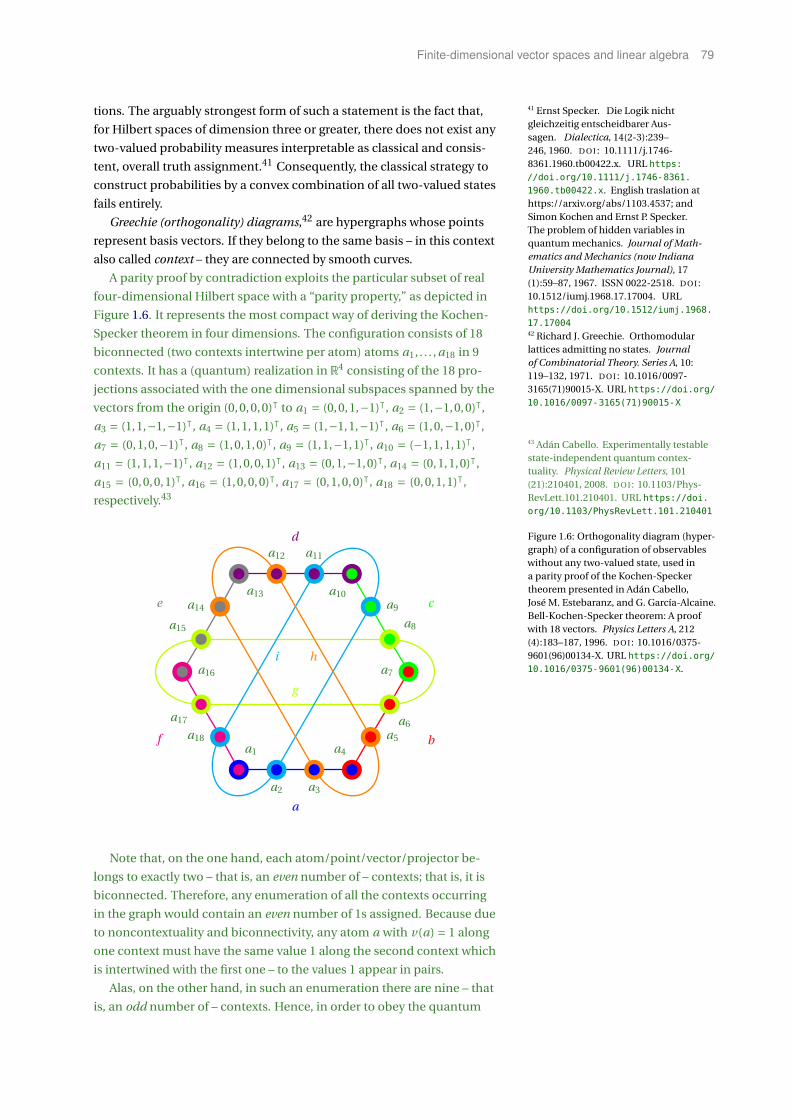
Finite-dimensional vector spaces and linear algebra 79

tions. The arguably strongest form of such a statement is the fact that,

for Hilbert spaces of dimension three or greater, there does not exist any

two-valued probability measures interpretable as classical and consis-

tent, overall truth assignment.41 Consequently, the classical strategy to

41 Ernst Specker. Die Logik nichtgleichzeitig entscheidbarer Aus-sagen. Dialectica, 14(2-3):239–246, 1960. D O I : 10.1111/j.1746-8361.1960.tb00422.x. URL https:

//doi.org/10.1111/j.1746-8361.

1960.tb00422.x. English traslation athttps://arxiv.org/abs/1103.4537; andSimon Kochen and Ernst P. Specker.The problem of hidden variables inquantum mechanics. Journal of Math-ematics and Mechanics (now IndianaUniversity Mathematics Journal), 17(1):59–87, 1967. ISSN 0022-2518. D O I :10.1512/iumj.1968.17.17004. URLhttps://doi.org/10.1512/iumj.1968.

17.17004

construct probabilities by a convex combination of all two-valued states

fails entirely.

Greechie (orthogonality) diagrams,42 are hypergraphs whose points

42 Richard J. Greechie. Orthomodularlattices admitting no states. Journalof Combinatorial Theory. Series A, 10:119–132, 1971. D O I : 10.1016/0097-3165(71)90015-X. URL https://doi.org/

10.1016/0097-3165(71)90015-X

represent basis vectors. If they belong to the same basis – in this context

also called context – they are connected by smooth curves.

A parity proof by contradiction exploits the particular subset of real

four-dimensional Hilbert space with a “parity property,” as depicted in

Figure 1.6. It represents the most compact way of deriving the Kochen-

Specker theorem in four dimensions. The configuration consists of 18

biconnected (two contexts intertwine per atom) atoms a1, . . . , a18 in 9

contexts. It has a (quantum) realization in R4 consisting of the 18 pro-

jections associated with the one dimensional subspaces spanned by the

vectors from the origin (0,0,0,0)ᵀ to a1 = (0,0,1,−1)ᵀ, a2 = (1,−1,0,0)ᵀ,

a3 = (1,1,−1,−1)ᵀ, a4 = (1,1,1,1)ᵀ, a5 = (1,−1,1,−1)ᵀ, a6 = (1,0,−1,0)ᵀ,

a7 = (0,1,0,−1)ᵀ, a8 = (1,0,1,0)ᵀ, a9 = (1,1,−1,1)ᵀ, a10 = (−1,1,1,1)ᵀ,

a11 = (1,1,1,−1)ᵀ, a12 = (1,0,0,1)ᵀ, a13 = (0,1,−1,0)ᵀ, a14 = (0,1,1,0)ᵀ,

a15 = (0,0,0,1)ᵀ, a16 = (1,0,0,0)ᵀ, a17 = (0,1,0,0)ᵀ, a18 = (0,0,1,1)ᵀ,

respectively.43

43 Adán Cabello. Experimentally testablestate-independent quantum contex-tuality. Physical Review Letters, 101(21):210401, 2008. D O I : 10.1103/Phys-RevLett.101.210401. URL https://doi.

org/10.1103/PhysRevLett.101.210401

a

b

c

d

e

f

i h

g

a1

a2 a3

a4

a5

a6

a7

a8

a9

a10

a11a12

a13a14

a15

a16

a17

a18

Figure 1.6: Orthogonality diagram (hyper-graph) of a configuration of observableswithout any two-valued state, used ina parity proof of the Kochen-Speckertheorem presented in Adán Cabello,José M. Estebaranz, and G. García-Alcaine.Bell-Kochen-Specker theorem: A proofwith 18 vectors. Physics Letters A, 212(4):183–187, 1996. D O I : 10.1016/0375-9601(96)00134-X. URL https://doi.org/

10.1016/0375-9601(96)00134-X.

Note that, on the one hand, each atom/point/vector/projector be-

longs to exactly two – that is, an even number of – contexts; that is, it is

biconnected. Therefore, any enumeration of all the contexts occurring

in the graph would contain an even number of 1s assigned. Because due

to noncontextuality and biconnectivity, any atom a with v(a) = 1 along

one context must have the same value 1 along the second context which

is intertwined with the first one – to the values 1 appear in pairs.

Alas, on the other hand, in such an enumeration there are nine – that

is, an odd number of – contexts. Hence, in order to obey the quantum

80 Mathematical Methods of Theoretical Physics

predictions, any two-valued state (interpretable as truth assignment)

would need to have an odd number of 1s – exactly one for each context.

Therefore, there cannot exist any two-valued state on Kochen-Specker

type graphs with the “parity property.”

More concretely, note that, within each one of those 9 contexts, the

sum of any state on the atoms of that context must add up to 1. That is,

one obtains a system of 9 equations

v(a) = v(a1)+ v(a2)+ v(a3)+ v(a4) = 1,

v(b) = v(a4)+ v(a5)+ v(a6)+ v(a7) = 1,

v(c) = v(a7)+ v(a8)+ v(a9)+ v(a10) = 1,

v(d) = v(a10)+ v(a11)+ v(a12)+ v(a13) = 1,

v(e) = v(a13)+ v(a14)+ v(a15)+ v(a16) = 1,

v( f ) = v(a16)+ v(a17)+ v(a18)+ v(a1) = 1,

v(g ) = v(a6)+ v(a8)+ v(a15)+ v(a17) = 1,

v(h) = v(a3)+ v(a5)+ v(a12)+ v(a14) = 1,

v(i ) = v(a2)+ v(a9)+ v(a11)+ v(a18) = 1. (1.290)

By summing up the left hand side and the right hand sides of the equa-

tions, and since all atoms are biconnected, one obtains

2

[18∑

i=1v(ai )

]= 9. (1.291)

Because v(ai ) ∈ 0,1 the sum in (1.291) must add up to some natural

number M . Therefore, Equation (1.291) is impossible to solve in the

domain of natural numbers, as on the left and right-hand sides, there

appear even (2M) and odd (9) numbers, respectively.

Of course, one could also prove the nonexistence of any two-valued

state (interpretable as truth assignment) by exhaustive attempts

(possibly exploiting symmetries) to assign values 0s and 1s to the

atoms/points/vectors/projectors occurring in the graph in such a way

that both the quantum predictions as well as context independence are

satisfied. This latter method needs to be applied in cases with Kochen-

Specker type diagrams (hypergraphs) without the “parity property;” such

as in the original Kochen-Specker proof.44

44 Simon Kochen and Ernst P. Specker.The problem of hidden variables inquantum mechanics. Journal of Math-ematics and Mechanics (now IndianaUniversity Mathematics Journal), 17(1):59–87, 1967. ISSN 0022-2518. D O I :10.1512/iumj.1968.17.17004. URLhttps://doi.org/10.1512/iumj.1968.

17.17004

Note also that in this original paper Kochen and Specker pointed

out (in Theorem 0 on page 67) that a much smaller set of quantum

propositions in intertwining contexts (orthonormal basis) suffices to

prove nonclassicality: all it needs is a configuration with a nonseparating

set of two-valued states; that is, there exist at least two observables with

the same truth assignments for all such truth assignments – pointedly

stated, the classical truth assignments are unable to separate between

those two observables.

Any such construction is usually based on a succession of auxiliary

gadget graphs45 stitched together to yield the desired property. Thereby,

45 W. T. Tutte. A short proof of the factortheorem for finite graphs. CanadianJournal of Mathematics, 6:347–352,1954. D O I : 10.4153/CJM-1954-033-3. URL https://doi.org/10.4153/

CJM-1954-033-3; Jácint Szabó. Goodcharacterizations for some degreeconstrained subgraphs. Journal ofCombinatorial Theory, Series B, 99(2):436–446, 2009. ISSN 0095-8956. D O I :10.1016/j.jctb.2008.08.009. URL https://

doi.org/10.1016/j.jctb.2008.08.009;and Ravishankar Ramanathan, MonikaRosicka, Karol Horodecki, StefanoPironio, Michal Horodecki, and PawelHorodecki. Gadget structures in proofs ofthe Kochen-Specker theorem, 2018. URLhttps://arxiv.org/abs/1807.00113

gadgets are formed from gadgets of ever-increasing size and functional

performance (see also Chapter 12 of Ref.46):

46 Karl Svozil. Physical [A]Causality.Determinism, Randomness and UncausedEvents. Springer, Cham, Berlin, Heidelberg,New York, 2018a. D O I : 10.1007/978-3-319-70815-7. URL https://doi.org/10.

1007/978-3-319-70815-7

1. 0th order gadget: a single context (aka clique/block/Boolean

(sub)algebra/maximal observable/orthonormal basis);

Finite-dimensional vector spaces and linear algebra 81

2. 1st order “firefly” gadget:] two contexts connected in a single inter-

twining atom;

3. 2nd order gadget: two 1st order firefly gadgets connected in a single

intertwining atom;

4. 3rd order house/pentagon/pentagram gadget: one firefly and one

2nd order gadget connected in two intertwining atoms to form a cyclic

orthogonality diagram (hypergraph);

5. 4rth order true-implies-false (TIFS)/01-(maybe better 10)-gadget:

e.g., a Specker bug consisting of two pentagon gadgets connected by

an entire context; as well as extensions thereof to arbitrary angles for

terminal (“extreme”) points;

6. 5th order true-implies-true (TITS)/11-gadget: e.g., Kochen and

Specker’s Γ1, consisting of one 10-gadget and one firefly gadget,

connected at the respective terminal points;

7. 6th order gadget: e.g., Kochen and Specker’s Γ3, consisting of a combo

of two 11-gadgets, connected by their common firefly gadgets;

8. 7th order construction: consisting of one 10- and one 11-gadget,

with identical terminal points serving as constructions of Pitowsky’s

principle of indeterminacy; 47 47 Itamar Pitowsky. Infinite and finiteGleason’s theorems and the logic ofindeterminacy. Journal of MathematicalPhysics, 39(1):218–228, 1998. D O I :10.1063/1.532334. URL https://doi.

org/10.1063/1.532334; Alastair A.Abbott, Cristian S. Calude, and Karl Svozil.A variant of the Kochen-Specker theoremlocalising value indefiniteness. Journalof Mathematical Physics, 56(10):102201,2015. D O I : 10.1063/1.4931658. URL https:

//doi.org/10.1063/1.4931658; andKarl Svozil. New forms of quantum valueindefiniteness suggest that incompatibleviews on contexts are epistemic. Entropy,20(6):406(22), 2018b. ISSN 1099-4300.D O I : 10.3390/e20060406. URL https:

//doi.org/10.3390/e20060406

9. 8th order construction: concatenation of (10- and) 11-gadgets

pasted/stitched together to form a graph used for proofs of the

Kochen-Specker theorem; e.g., Kochen and Specker’s Γ2.

b

Multilinear algebra and tensors 83

2Multilinear algebra and tensors

In the following chapter multilinear extensions of linear functionals will

be discussed. Tensors will be introduced as multilinear forms, and their

transformation properties will be derived.

For many physicists, the following derivations might appear confusing

and overly formalistic as they might have difficulties to “see the forest

for the trees.” For those, a brief overview sketching the most important

aspects of tensors might serve as a first orientation.

Let us start by defining, or rather declaring or supposing the following:

basis vectors of some given (base) vector space are said to “(co-)vary.”

This is just a “fixation,” a designation of notation; important insofar as it

implies that the respective coordinates, as well as the dual basis vectors

“contra-vary;” and the coordinates of dual space vectors “co-vary.”

Based on this declaration or rather convention – that is, relative to

the behavior with respect to variations of scales of the reference axes

(the basis vectors) in the base vector space – there exist two important

categories: entities which co-vary, and entities which vary inversely, that

is, contra-vary, with such changes.

• Contravariant entities such as vectors in the base vector space: These

vectors of the base vector space are called contravariant because

their components contra-vary (that is, vary inversely) with respect to

variations of the basis vectors. By identification, the components of

contravariant vectors (or tensors) are also contravariant. In general,

a multilinear form on a vector space is called contravariant if its

components (coordinates) are contravariant; that is, they contra-vary

with respect to variations of the basis vectors.

• Covariant entities such as vectors in the dual space: The vectors of the The dual space is spanned by all linearfunctionals on that vector space (cf.Section 1.8 on page 15).

dual space are called covariant because their components contra-vary

with respect to variations of the basis vectors of the dual space, which

in turn contra-vary with respect to variations of the basis vectors of

the base space. Thereby the double contra-variations (inversions)

cancel out, so that effectively the vectors of the dual space co-vary

with the vectors of the basis of the base vector space. By identification,

the components of covariant vectors (or tensors) are also covariant.

In general, a multilinear form on a vector space is called covariant if

84 Mathematical Methods of Theoretical Physics

its components (coordinates) are covariant; that is, they co-vary with

respect to variations of the basis vectors of the base vector space.

• Covariant and contravariant indices will be denoted by subscripts

(lower indices) and superscripts (upper indices), respectively.

• Covariant and contravariant entities transform inversely. Informally,

this is due to the fact that their changes must compensate each

other, as covariant and contravariant entities are “tied together” by

some invariant (id)entities such as vector encoding and dual basis

formation.

• Covariant entities can be transformed into contravariant ones by the

application of metric tensors, and, vice versa, by the inverse of metric

tensors.

2.1 Notation

In what follows, vectors and tensors will be encoded in terms of indexed

coordinates or components (with respect to a specific basis). The biggest

advantage is that such coordinates or components are scalars which can

be exchanged and rearranged according to commutativity, associativity,

and distributivity, as well as differentiated.

Let us consider the vector space V = Rn of dimension n. A covariant For a more systematic treatment, seefor instance, the introductions EbergardKlingbeil. Tensorrechnung für Ingenieure.Bibliographisches Institut, Mannheim,1966 and Hans Jörg Dirschmid. Tensorenund Felder. Springer, Vienna, 1996.

basis B = e1,e2, . . . ,en of V consists of n covariant basis vectors ei . A

For a detailed explanation of covarianceand contravariance, see Section 2.2 onpage 85.

contravariant basis B∗ = e∗1 ,e∗2 , . . . ,e∗n = e1,e2, . . . ,en of the dual space

V ∗ (cf. Section 1.8.1 on page 17) consists of n basis vectors e∗i , where

e∗i = ei is just a different notation.

Every contravariant vector x ∈ V can be coded by, or expressed in

terms of, its contravariant vector components x1, x2, . . . , xn ∈ R by x =∑ni=1 xi ei . Likewise, every covariant vector x ∈ V ∗ can be coded by, or

expressed in terms of, its covariant vector components x1, x2, . . . , xn ∈ Rby x =∑n

i=1 xi e∗i =∑ni=1 xi ei . Note that in both covariant and con-

travariant cases the upper-lower pairings“ ·i ·i ” and “ ·i ·i ”of the indices match.

Suppose that there are k arbitrary contravariant vectors x1,x2, . . . ,xk

in V which are indexed by a subscript (lower index). This lower index

should not be confused with a covariant lower index. Every such vector

x j , 1 ≤ j ≤ k has contravariant vector components x1 j

j , x2 j

j , . . . , xn j

j ∈ Rwith respect to a particular basis B such that This notation “x

i jj ” for the i th component

of the j th vector is redundant as itrequires two indices j ; we could have

just denoted it by “xi j .” The lower indexj does not correspond to any covariantentity but just indexes the j th vector x j .

x j =n∑

i j =1x

i j

j ei j . (2.1)

Likewise, suppose that there are k arbitrary covariant vectors

x1,x2, . . . ,xk in the dual space V ∗ which are indexed by a superscript

(upper index). This upper index should not be confused with a con-

travariant upper index. Every such vector x j , 1 ≤ j ≤ k has covariant

vector components x j1 j

, x j2 j

, . . . , x jn j

∈ Rwith respect to a particular basis

B∗ such that Again, this notation “xji j

” for the i th

component of the j th vector is redundantas it requires two indices j ; we could havejust denoted it by “xi j

.” The upper index j

does not correspond to any contravariantentity but just indexes the j th vector x j .

x j =n∑

i j =1x j

i jei j . (2.2)

Tensors are constant with respect to variations of points of Rn . In

contradistinction, tensor fields depend on points of Rn in a nontrivial

Multilinear algebra and tensors 85

(nonconstant) way. Thus, the components of a tensor field depend on the

coordinates. For example, the contravariant vector defined by the coor-

dinates(5.5,3.7, . . . ,10.9

)ᵀwith respect to a particular basis B is a tensor;

while, again with respect to a particular basis B,(sin x1,cos x2, . . . ,exn

)ᵀor

(x1, x2, . . . , xn

)ᵀ, which depend on the coordinates x1, x2, . . . , xn ∈R, are

tensor fields.

We adopt Einstein’s summation convention to sum over equal indices.

If not explained otherwise (that is, for orthonormal bases) those pairs

have exactly one lower and one upper index.

In what follows, the notations “x · y”, “(x, y)” and “⟨x | y⟩” will be used

synonymously for the scalar product or inner product. Note, however,

that the “dot notation x · y” may be a little bit misleading; for example,

in the case of the “pseudo-Euclidean” metric represented by the matrix

diag(+,+,+, · · · ,+,−), it is no more the standard Euclidean dot product

diag(+,+,+, · · · ,+,+).

2.2 Change of basis

2.2.1 Transformation of the covariant basis

Let B and B′ be two arbitrary bases of Rn . Then every vector fi of B′

can be represented as linear combination of basis vectors of B [see also

Eqs. (1.100) and (1.101)]:

fi =n∑

j=1a j

i e j , i = 1, . . . ,n. (2.3)

The matrix

A≡ a ji ≡

a1

1 a12 · · · a1

n

a21 a2

2 · · · a2n

......

. . ....

an1 an

2 · · · ann

. (2.4)

is called the transformation matrix. As defined in (1.3) on page 4, the

second (from the left to the right), rightmost (in this case lower) index i

varying in row vectors is the column index; and, the first, leftmost (in this

case upper) index j varying in columns is the row index, respectively.

Note that, as discussed earlier, it is necessary to fix a convention for

the transformation of the covariant basis vectors discussed on page 31.

This then specifies the exact form of the (inverse, contravariant) transfor-

mation of the components or coordinates of vectors.

Perhaps not very surprisingly, compared to the transformation (2.3)

yielding the “new” basis B′ in terms of elements of the “old” basis B, a

transformation yielding the “old” basis B in terms of elements of the

“new” basis B′ turns out to be just the inverse “back” transformation of

the former: substitution of (2.3) yields

ei =n∑

j=1a′ j

i f j =n∑

j=1a′ j

i

n∑k=1

akj ek =

n∑k=1

(n∑

j=1a′ j

i akj

)ek , (2.5)

which, due to the linear independence of the basis vectors ei of B, can

86 Mathematical Methods of Theoretical Physics

only be satisfied if

akj a′ j

i = δki or AA′ = I. (2.6)

Thus A′ is the inverse matrix A−1 of A. In index notation,

a′ ji = (a−1)

ji , (2.7)

and

ei =n∑

j=1(a−1)

ji f j . (2.8)

2.2.2 Transformation of the contravariant coordinates

Consider an arbitrary contravariant vector x ∈ Rn in two basis represen-

tations: (i) with contravariant components xi with respect to the basis

B, and (ii) with y i with respect to the basis B′. Then, because both coor-

dinates with respect to the two different bases have to encode the same

vector, there has to be a “compensation-of-scaling” such that

x =n∑

i=1xi ei =

n∑i=1

y i fi . (2.9)

Insertion of the basis transformation (2.3) and relabelling of the indices

i ↔ j yields

x =n∑

i=1xi ei =

n∑i=1

y i fi =n∑

i=1y i

n∑j=1

a ji e j

=n∑

i=1

n∑j=1

a ji y i e j =

n∑j=1

[n∑

i=1a j

i y i

]e j =

n∑i=1

[n∑

j=1ai

j y j

]ei . (2.10)

A comparison of coefficients yields the transformation laws of vector

components [see also Equation (1.109)]

xi =n∑

j=1ai

j y j . (2.11)

In the matrix notation introduced in Equation (1.19) on page 12, (2.11)

can be written as

X =AY . (2.12)

A similar “compensation-of-scaling” argument using (2.8) yields the

transformation laws for

y j =n∑

i=1(a−1) j

i xi (2.13)

with respect to the covariant basis vectors. In the matrix notation in-

troduced in Equation (1.19) on page 12, (2.13) can simply be written as

Y = (A−1) X . (2.14)

If the basis transformations involve nonlinear coordinate changes

– such as from the Cartesian to the polar or spherical coordinates dis-

cussed later – we have to employ differentials

d x j =n∑

i=1a j

i d y i , (2.15)

Multilinear algebra and tensors 87

so that, by partial differentiation,

a ji = ∂x j

∂y i. (2.16)

By assuming that the coordinate transformations are linear, aij can be

expressed in terms of the coordinates x j

a ji = x j

y i. (2.17)

Likewise,

d y j =n∑

i=1(a−1)

ji d xi , (2.18)

so that, by partial differentiation,

(a−1)j

i =∂y j

∂xi= J j i , (2.19)

where J j i = ∂y j

∂xi stands for the j th row and i th column component of the

Jacobian matrix

J (x1, x2, . . . , xn)def=

(∂∂x1 · · · ∂

∂xn

)×

y1

...

yn

≡

∂y1

∂x1 · · · ∂y1

∂xn

.... . .

...∂yn

∂x1 · · · ∂yn

∂xn

. (2.20)

Potential confusingly, its determinant

Jdef=∂(

y1, . . . , yn)

∂(x1, . . . , xn

) = det

∂y1

∂x1 · · · ∂y1

∂xn

.... . .

...∂yn

∂x1 · · · ∂yn

∂xn

(2.21)

is also often referred to as “the Jacobian.”

2.2.3 Transformation of the contravariant (dual) basis

Consider again, as a starting point, a covariant basis B = e1,e2, . . . ,en

consisting of n basis vectors ei . A contravariant basis can be defined

by identifying it with the dual basis introduced earlier in Section 1.8.1

on page 17, in particular, Equation (1.39). Thus a contravariant basis

B∗ = e1,e2, . . . ,en is a set of n covariant basis vectors ei which satisfy

Eqs. (1.39)-(1.41)

e j (ei ) = qei ,e j

y=r

ei ,e∗jz= δ j

i = δi j . (2.22)

In terms of the bra-ket notation, (2.22) somewhat superficially trans-

forms into (a formal justification for this identification is the Riesz

representation theorem)

q|ei ⟩,⟨e j |y= ⟨e j |ei ⟩ = δi j . (2.23)

Furthermore, the resolution of identity (1.127) can be rewritten as

In =n∑

i=1|ei ⟩⟨ei |. (2.24)

88 Mathematical Methods of Theoretical Physics

As demonstrated earlier in Equation (1.42) the vectors e∗i = ei of the

dual basis can be used to “retrieve” the components of arbitrary vectors

x =∑j x j e j through

ei (x) = ei

(∑i

x j e j

)=∑

ix j ei (

e j)=∑

ix jδi

j = xi . (2.25)

Likewise, the basis vectors ei of the “base space” can be used to obtain

the coordinates of any dual vector x =∑j x j e j through

ei (x) = ei

(∑i

x j e j

)=∑

ix j ei

(e j

)=∑

ix jδ

ji = xi . (2.26)

As also noted earlier, for orthonormal bases and Euclidean scalar (dot)

products (the coordinates of) the dual basis vectors of an orthonormal

basis can be coded identically as (the coordinates of) the original basis

vectors; that is, in this case, (the coordinates of) the dual basis vectors are

just rearranged as the transposed form of the original basis vectors.

In the same way as argued for changes of covariant bases (2.3), that

is, because every vector in the new basis of the dual space can be repre-

sented as a linear combination of the vectors of the original dual basis –

we can make the formal Ansatz:

f j =∑i

b ji ei , (2.27)

where B ≡ b ji is the transformation matrix associated with the con-

travariant basis. How is b, the transformation of the contravariant basis,

related to a, the transformation of the covariant basis?

Before answering this question, note that, again – and just as the

necessity to fix a convention for the transformation of the covariant

basis vectors discussed on page 31 – we have to choose by convention the

way transformations are represented. In particular, if in (2.27) we would

have reversed the indices b ji ↔ bi

j , thereby effectively transposing

the transformation matrix B, this would have resulted in a changed

(transposed) form of the transformation laws, as compared to both the

transformation a of the covariant basis, and of the transformation of

covariant vector components.

By exploiting (2.22) twice we can find the connection between the

transformation of covariant and contravariant basis elements and

thus tensor components; that is (by assuming Einstein’s summation

convention we are omitting to write sums explicitly),

δji = δi j = f j (fi ) = q

fi , f jy= q

aki ek ,b j

l ely=

= aki b j

lq

ek ,ely= ak

i b jlδ

lk = ak

i b jlδkl = b j

k aki . (2.28)

Therefore,

B=A−1, or b ji =

(a−1) j

i , (2.29)

and

f j =∑i

(a−1) j

i ei . (2.30)

In short, by comparing (2.30) with (2.13), we find that the vectors of

the contravariant dual basis transform just like the components of

contravariant vectors.

Multilinear algebra and tensors 89

2.2.4 Transformation of the covariant coordinates

For the same, compensatory, reasons yielding the “contra-varying” trans-

formation of the contravariant coordinates with respect to variations

of the covariant bases [reflected in Eqs. (2.3), (2.13), and (2.19)] the

coordinates with respect to the dual, contravariant, basis vectors, trans-

form covariantly. We may therefore say that “basis vectors ei , as well as

dual components (coordinates) xi vary covariantly.” Likewise, “vector

components (coordinates) xi , as well as dual basis vectors e∗i = ei vary

contra-variantly.”

A similar calculation as for the contravariant components (2.10) yields

a transformation for the covariant components:

x =n∑

i=1x j e j =

n∑i=1

yi fi =n∑

i=1yi

n∑j=1

bij e j =

n∑j=1

(n∑

i=1bi

j yi

)e j . (2.31)

Thus, by comparison we obtain

xi =n∑

j=1b j

i y j =n∑

j=1

(a−1) j

i y j , and

yi =n∑

j=1

(b−1) j

i x j =n∑

j=1a j

i x j . (2.32)

In short, by comparing (2.32) with (2.3), we find that the components of

covariant vectors transform just like the vectors of the covariant basis

vectors of “base space.”

2.2.5 Orthonormal bases

For orthonormal bases of n-dimensional Hilbert space,

δji = ei ·e j if and only if ei = ei for all 1 ≤ i , j ≤ n. (2.33)

Therefore, the vector space and its dual vector space are “identical” in

the sense that the coordinate tuples representing their bases are identical

(though relatively transposed). That is, besides transposition, the two

bases are identical

B≡B∗ (2.34)

and formally any distinction between covariant and contravariant

vectors becomes irrelevant. Conceptually, such a distinction persists,

though. In this sense, we might “forget about the difference between

covariant and contravariant orders.”

2.3 Tensor as multilinear form

A multilinear form α : V k 7→ R or C is a map from (multiple) arguments

xi which are elements of some vector space V into some scalars in R or C,

satisfying

α(x1,x2, . . . , Ay+Bz, . . . ,xk ) = Aα(x1,x2, . . . ,y, . . . ,xk )

+Bα(x1,x2, . . . ,z, . . . ,xk ) (2.35)

for every one of its (multi-)arguments.

90 Mathematical Methods of Theoretical Physics

Note that linear functionals on V , which constitute the elements of the

dual space V ∗ (cf. Section 1.8 on page 15) is just a particular example of a

multilinear form – indeed rather a linear form – with just one argument, a

vector in V .

In what follows we shall concentrate on real-valued multilinear forms

which map k vectors in Rn into R.

2.4 Covariant tensors

Mind the notation introduced earlier; in particular in Eqs. (2.1) and (2.2).

A covariant tensor of rank k

α : V k 7→R (2.36)

is a multilinear form

α(x1,x2, . . . ,xk ) =n∑

i1=1

n∑i2=1

· · ·n∑

ik=1xi1

1 xi22 . . . xik

k α(ei1 ,ei2 , . . . ,eik ). (2.37)

The

Ai1i2···ik

def= α(ei1 ,ei2 , . . . ,eik ) (2.38)

are the covariant components or covariant coordinates of the tensor α

with respect to the basis B.

Note that, as each of the k arguments of a tensor of type (or rank)

k has to be evaluated at each of the n basis vectors e1,e2, . . . ,en in an

n-dimensional vector space, Ai1i2···ik has nk coordinates.

To prove that tensors are multilinear forms, insert

α(x1,x2, . . . , Ax1j +Bx2

j , . . . ,xk )

=n∑

i1=1

n∑i2=1

· · ·n∑

ik=1xii

1 xi22 . . . [A(x1)

i j

j +B(x2)i j

j ] . . . xikk α(ei1 ,ei2 , . . . ,ei j , . . . ,eik )

= An∑

i1=1

n∑i2=1

· · ·n∑

ik=1xii

1 xi22 . . . (x1)

i j

j . . . xikk α(ei1 ,ei2 , . . . ,ei j , . . . ,eik )

+Bn∑

i1=1

n∑i2=1

· · ·n∑

ik=1xii

1 xi22 . . . (x2)

i j

j . . . xikk α(ei1 ,ei2 , . . . ,ei j , . . . ,eik )

= Aα(x1,x2, . . . ,x1j , . . . ,xk )+Bα(x1,x2, . . . ,x2

j , . . . ,xk )

2.4.1 Transformation of covariant tensor components

Because of multilinearity and by insertion into (2.3),

α(f j1 , f j2 , . . . , f jk ) =α(

n∑i1=1

ai1j1 ei1 ,

n∑i2=1

ai2j2 ei2 , . . . ,

n∑ik=1

aikjk eik

)

=n∑

i1=1

n∑i2=1

· · ·n∑

ik=1ai1

j1 ai2j2 · · ·aik

jkα(ei1 ,ei2 , . . . ,eik ) (2.39)

or

A′j1 j2··· jk

=n∑

i1=1

n∑i2=1

· · ·n∑

ik=1ai1

j1 ai2j2 · · ·aik

jk Ai1i2...ik . (2.40)

In effect, this yields a transformation factor “aij ” for every “old index

i ” and “new index j .”

Multilinear algebra and tensors 91

2.5 Contravariant tensors

Recall the inverse scaling of contravariant vector coordinates with re-

spect to covariantly varying basis vectors. Recall further that the dual

base vectors are defined in terms of the base vectors by a kind of “inver-

sion” of the latter, as expressed by [ei ,e∗j ] = δi j in Equation (1.39). Thus,

by analogy, it can be expected that similar considerations apply to the

scaling of dual base vectors with respect to the scaling of covariant base

vectors: in order to compensate those scale changes, dual basis vectors

should contra-vary, and, again analogously, their respective dual coor-

dinates, as well as the dual vectors, should vary covariantly. Thus, both

vectors in the dual space, as well as their components or coordinates, will

be called covariant vectors, as well as covariant coordinates, respectively.

2.5.1 Definition of contravariant tensors

The entire tensor formalism developed so far can be transferred and

applied to define contravariant tensors as multilinear forms with con-

travariant components

β : V ∗k 7→R (2.41)

by

β(x1,x2, . . . ,xk ) =n∑

i1=1

n∑i2=1

· · ·n∑

ik=1x1

i1x2

i2. . . xk

ikβ(ei1 ,ei2 , . . . ,eik ). (2.42)

By definition

B i1i2···ik =β(ei1 ,ei2 , . . . ,eik ) (2.43)

are the contravariant components of the contravariant tensor β with

respect to the basis B∗.

2.5.2 Transformation of contravariant tensor components

The argument concerning transformations of covariant tensors and

components can be carried through to the contravariant case. Hence, the

contravariant components transform as

β(f j1 , f j2 , . . . , f jk ) =β(

n∑i1=1

b j1i1 ei1 ,

n∑i2=1

b j2i2 ei2 , . . . ,

n∑ik=1

b jkik eik

)

=n∑

i1=1

n∑i2=1

· · ·n∑

ik=1b j1

i1 b j2i2 · · ·b jk

ikβ(ei1 ,ei2 , . . . ,eik ) (2.44)

or

B ′ j1 j2··· jk =n∑

i1=1

n∑i2=1

· · ·n∑

ik=1b j1

i1 b j2i2 · · ·b jk

ik B i1i2...ik . (2.45)

Note that, by Equation (2.29), b ji =

(a−1

) ji . In effect, this yields a

transformation factor “(a−1

) ji ” for every “old index i ” and “new index j .”

92 Mathematical Methods of Theoretical Physics

2.6 General tensor

A (general) Tensor T can be defined as a multilinear form on the r -fold

product of a vector space V , times the s-fold product of the dual vector

space V ∗. If all r components appear on the left and all s components

right side – in general covariant and contravariant components can have

mixed orders – one can denote this by

T : (V )r × (V ∗)s = V ×·· ·×V︸ ︷︷ ︸

r copies

×V ∗×·· ·×V ∗︸ ︷︷ ︸s copies

7→ F. (2.46)

Most commonly, the scalar field Fwill be identified with the set R of reals,

or with the set C of complex numbers. Thereby, r is called the covariant

order, and s is called the contravariant order of T . A tensor of covariant

order r and contravariant order s is then pronounced a tensor of type (or

rank) (r , s). By convention, covariant indices are denoted by subscripts,

whereas the contravariant indices are denoted by superscripts.

With the standard, “inherited” addition and scalar multiplication, the

set T sr of all tensors of type (r , s) forms a linear vector space.

Note that a tensor of type (1,0) is called a covariant vector , or just a

vector. A tensor of type (0,1) is called a contravariant vector.

Tensors can change their type by the invocation of the metric tensor.

That is, a covariant tensor (index) i can be made into a contravariant

tensor (index) j by summing over the index i in a product involving

the tensor and g i j . Likewise, a contravariant tensor (index) i can be

made into a covariant tensor (index) j by summing over the index i in a

product involving the tensor and gi j .

Under basis or other linear transformations, covariant tensors with

index i transform by summing over this index with (the transformation

matrix) aij . Contravariant tensors with index i transform by summing

over this index with the inverse (transformation matrix) (a−1)ij.

2.7 Metric

A metric or metric tensor g is a measure of distance between two points in

a vector space.

2.7.1 Definition

Formally, a metric, or metric tensor, can be defined as a functional

g : Rn ×Rn 7→Rwhich maps two vectors (directing from the origin to the

two points) into a scalar with the following properties:

• g is symmetric; that is, g (x,y) = g (y,x);

• g is bilinear; that is, g (αx+βy,z) =αg (x,z)+βg (y,z) (due to symmetry

g is also bilinear in the second argument);

• g is nondegenerate; that is, for every x ∈ V , x 6= 0, there exists a y ∈ V

such that g (x,y) 6= 0.

Multilinear algebra and tensors 93

2.7.2 Construction from a scalar product

In real Hilbert spaces the metric tensor can be defined via the scalar

product by

gi j = ⟨ei | e j ⟩. (2.47)

and

g i j = ⟨ei | e j ⟩. (2.48)

For orthonormal bases, the metric tensor can be represented as a

Kronecker delta function, and thus remains form invariant. Moreover, its

covariant and contravariant components are identical; that is, gi j = δi j =δi

j = δji = δi j = g i j .

2.7.3 What can the metric tensor do for you?

We shall see that with the help of the metric tensor we can “raise and

lower indices;” that is, we can transform lower (covariant) indices into

upper (contravariant) indices, and vice versa. This can be seen as follows.

Because of linearity, any contravariant basis vector ei can be written as

a linear sum of covariant (transposed, but we do not mark transposition

here) basis vectors:

ei = Ai j e j . (2.49)

Then,

g i k = ⟨ei |ek⟩ = ⟨Ai j e j |ek⟩ = Ai j ⟨e j |ek⟩ = Ai jδkj = Ai k (2.50)

and thus

ei = g i j e j (2.51)

and, by a similar argument,

ei = gi j e j . (2.52)

This property can also be used to raise or lower the indices not only of

basis vectors but also of tensor components; that is, to change from con-

travariant to covariant and conversely from covariant to contravariant.

For example,

x = xi ei = xi gi j e j = x j e j , (2.53)

and hence x j = xi gi j .

What is g ij ? A straightforward calculation yields, through insertion

of Eqs. (2.47) and (2.48), as well as the resolution of unity (in a modified

form involving upper and lower indices; cf. Section 1.14 on page 35),

g ij = g i k gk j = ⟨ei | ek⟩⟨ek |︸ ︷︷ ︸

I

e j ⟩ = ⟨ei | e j ⟩ = δij = δi j . (2.54)

A similar calculation yields gij = δi j .

The metric tensor has been defined in terms of the scalar product.

The converse can be true as well. (Note, however, that the metric need

not be positive.) In Euclidean space with the dot (scalar, inner) product

the metric tensor represents the scalar product between vectors: let

94 Mathematical Methods of Theoretical Physics

x = xi ei ∈ Rn and y = y j e j ∈ Rn be two vectors. Then (“ᵀ” stands for the

transpose),

x ·y ≡ (x,y) ≡ ⟨x | y⟩ = xi ei · y j e j = xi y j ei ·e j = xi y j gi j = xᵀg y . (2.55)

It also characterizes the length of a vector: in the above equation, set

y = x. Then,

x ·x ≡ (x,x) ≡ ⟨x | x⟩ = xi x j gi j ≡ xᵀg x, (2.56)

and thus, if the metric is positive definite,

‖x‖ =√

xi x j gi j =√

xᵀg x. (2.57)

The square of the line element or length element d s = ‖dx‖ of an

infinitesimal vector dx is

d s2 = gi j d xi d x j = dxᵀg dx. (2.58)

In (special) relativity with indefinite (Minkowski) metric, d s2, or

its finite difference form ∆s2, is used to define timelike, lightlike and

spacelike distances: with gi j = ηi j ≡ diag(1,1,1,−1), ∆s2 > 0 indicates

spacelike distances, ∆s2 < 0 indicates timelike distances, and ∆s2 > 0

indicates lightlike distances.

2.7.4 Transformation of the metric tensor

Insertion into the definitions and coordinate transformations (2.7) and

(2.8) yields

gi j = ei ·e j = a′li e′l ·a′m

j e′m = a′li a′m

j e′l ·e′m

= a′li a′m

j g ′l m = ∂y l

∂xi

∂ym

∂x jg ′

l m . (2.59)

Conversely, (2.3) as well as (2.17) yields

g ′i j = fi · f j = al

i el ·amj em = al

i amj el ·em

= ali am

j glm = ∂x l

∂y i

∂xm

∂y jgl m . (2.60)

If the geometry (i.e., the basis) is locally orthonormal, glm = δlm , then

g ′i j = ∂xl

∂y i∂xl∂y j .

Just to check consistency with Equation (2.54) we can compute, for

suitable differentiable coordinates X and Y ,

g ′i

j = fi · f j = ali el · (a−1)m

jem = al

i (a−1)mjel ·em

= ali (a−1)m

jδm

l = ali (a−1)l

j

= ∂x l

∂y i

∂yl

∂x j= ∂x l

∂x j

∂yl

∂yi= δl jδl i = δl

i . (2.61)

In terms of the Jacobian matrix defined in Equation (2.20) the metric

tensor in Equation (2.59) can be rewritten as

g = Jᵀg ′ J ≡ gi j = Jl i Jm j g ′lm . (2.62)

The metric tensor and the Jacobian (determinant) are thus related by

det g = (det Jᵀ)(det g ′)(det J ). (2.63)

If the manifold is embedded into an Euclidean space, then g ′l m = δlm and

g = Jᵀ J .

Multilinear algebra and tensors 95

2.7.5 Examples

In what follows a few metrics are enumerated and briefly commented.

For a more systematic treatment, see, for instance, Snapper and Troyer’s

Metric Affine geometry.1 1 Ernst Snapper and Robert J. Troyer.Metric Affine Geometry. Academic Press,New York, 1971

Note also that due to the properties of the metric tensor, its coordinate

representation has to be a symmetric matrix with nonzero diagonals. For

the symmetry g (x,y) = g (y,x) implies that gi j xi y j = gi j y i x j = gi j x j y i =g j i xi y j for all coordinate tuples xi and y j . And for any zero diagonal

entry (say, in the k’th position of the diagonal we can choose a nonzero

vector z whose coordinates are all zero except the k’th coordinate. Then

g (z,x) = 0 for all x in the vector space.

n-dimensional Euclidean space

g ≡ gi j = diag(1,1, . . . ,1︸ ︷︷ ︸n times

) (2.64)

One application in physics is quantum mechanics, where n stands

for the dimension of a complex Hilbert space. Some definitions can be

easily adapted to accommodate the complex numbers. E.g., axiom 5

of the scalar product becomes (x, y) = (x, y), where “(x, y)” stands for

complex conjugation of (x, y). Axiom 4 of the scalar product becomes

(x,αy) =α(x, y).

Lorentz plane

g ≡ gi j = diag(1,−1) (2.65)

Minkowski space of dimension n

In this case the metric tensor is called the Minkowski metric and is often

denoted by “η”:

η≡ ηi j = diag(1,1, . . . ,1︸ ︷︷ ︸n−1 times

,−1) (2.66)

One application in physics is the theory of special relativity, where

D = 4. Alexandrov’s theorem states that the mere requirement of the

preservation of zero distance (i.e., lightcones), combined with bijec-

tivity (one-to-oneness) of the transformation law yields the Lorentz

transformations.2

2 A. D. Alexandrov. On Lorentz transfor-mations. Uspehi Mat. Nauk., 5(3):187,1950; A. D. Alexandrov. A contribution tochronogeometry. Canadian Journal ofMath., 19:1119–1128, 1967; A. D. Alexan-drov. Mappings of spaces with familiesof cones and space-time transforma-tions. Annali di Matematica Pura edApplicata, 103:229–257, 1975. ISSN 0373-3114. D O I : 10.1007/BF02414157. URLhttps://doi.org/10.1007/BF02414157;A. D. Alexandrov. On the principles ofrelativity theory. In Classics of SovietMathematics. Volume 4. A. D. Alexan-drov. Selected Works, pages 289–318.1996; H. J. Borchers and G. C. Hegerfeldt.The structure of space-time transfor-mations. Communications in Math-ematical Physics, 28(3):259–266, 1972.URL http://projecteuclid.org/

euclid.cmp/1103858408; Walter Benz.Geometrische Transformationen. BIWissenschaftsverlag, Mannheim, 1992;June A. Lester. Distance preservingtransformations. In Francis Buekenhout,editor, Handbook of Incidence Geometry,pages 921–944. Elsevier, Amsterdam, 1995;and Karl Svozil. Conventions in relativitytheory and quantum mechanics. Foun-dations of Physics, 32:479–502, 2002. D O I :10.1023/A:1015017831247. URL https:

//doi.org/10.1023/A:1015017831247

Negative Euclidean space of dimension n

g ≡ gi j = diag(−1,−1, . . . ,−1︸ ︷︷ ︸n times

) (2.67)

Artinian four-space

g ≡ gi j = diag(+1,+1,−1,−1) (2.68)

96 Mathematical Methods of Theoretical Physics

General relativity

In general relativity, the metric tensor g is linked to the energy-mass

distribution. There, it appears as the primary concept when compared

to the scalar product. In the case of zero gravity, g is just the Minkowski

metric (often denoted by “η”) diag(1,1,1,−1) corresponding to “flat”

space-time.

The best known non-flat metric is the Schwarzschild metric

g ≡

(1−2m/r )−1 0 0 0

0 r 2 0 0

0 0 r 2 sin2θ 0

0 0 0 − (1−2m/r )

(2.69)

with respect to the spherical space-time coordinates r ,θ,φ, t .

Computation of the metric tensor of the circle of radius r

Consider the transformation from the standard orthonormal threedi-

mensional “Cartesian” coordinates x1 = x, x2 = y , into polar coordinates

x ′1 = r , x ′

2 = ϕ. In terms of r and ϕ, the Cartesian coordinates can be

written as

x1 = r cosϕ≡ x ′1 cos x ′

2,

x2 = r sinϕ≡ x ′1 sin x ′

2. (2.70)

Furthermore, since the basis we start with is the Cartesian orthonormal

basis, gi j = δi j ; therefore,

g ′i j =

∂x l

∂y i

∂xk

∂y jgl k = ∂x l

∂y i

∂xk

∂y jδlk = ∂x l

∂y i

∂xl

∂y j. (2.71)

More explicitely, we obtain for the coordinates of the transformed metric

tensor g ′

g ′11 =

∂x l

∂y1

∂xl

∂y1

= ∂(r cosϕ)

∂r

∂(r cosϕ)

∂r+ ∂(r sinϕ)

∂r

∂(r sinϕ)

∂r

= (cosϕ)2 + (sinϕ)2 = 1,

g ′12 =

∂x l

∂y1

∂xl

∂y2

= ∂(r cosϕ)

∂r

∂(r cosϕ)

∂ϕ+ ∂(r sinϕ)

∂r

∂(r sinϕ)

∂ϕ

= (cosϕ)(−r sinϕ)+ (sinϕ)(r cosϕ) = 0,

g ′21 =

∂x l

∂y2

∂xl

∂y1

= ∂(r cosϕ)

∂ϕ

∂(r cosϕ)

∂r+ ∂(r sinϕ)

∂ϕ

∂(r sinϕ)

∂r

= (−r sinϕ)(cosϕ)+ (r cosϕ)(sinϕ) = 0,

g ′22 =

∂x l

∂y2

∂xl

∂y2

= ∂(r cosϕ)

∂ϕ

∂(r cosϕ)

∂ϕ+ ∂(r sinϕ)

∂ϕ

∂(r sinϕ)

∂ϕ

= (−r sinϕ)2 + (r cosϕ)2 = r 2; (2.72)

Multilinear algebra and tensors 97

that is, in matrix notation,

g ′ =(

1 0

0 r 2

), (2.73)

and thus

(d s′)2 = g ′i j dx′i dx′ j = (dr )2 + r 2(dϕ)2. (2.74)

Computation of the metric tensor of the ball

Consider the transformation from the standard orthonormal threedi-

mensional “Cartesian” coordinates x1 = x, x2 = y , x3 = z, into spherical

coordinates x ′1 = r , x ′

2 = θ, x ′3 = ϕ. In terms of r ,θ,ϕ, the Cartesian

coordinates can be written as

x1 = r sinθcosϕ≡ x ′1 sin x ′

2 cos x ′3,

x2 = r sinθ sinϕ≡ x ′1 sin x ′

2 sin x ′3,

x3 = r cosθ ≡ x ′1 cos x ′

2. (2.75)

Furthermore, since the basis we start with is the Cartesian orthonormal

basis, gi j = δi j ; hence finally

g ′i j =

∂x l

∂y i

∂xl

∂y j≡ diag(1,r 2,r 2 sin2θ), (2.76)

and

(d s′)2 = (dr )2 + r 2(dθ)2 + r 2 sin2θ(dϕ)2. (2.77)

The expression d s2 = (dr )2 + r 2(dϕ)2 for polar coordinates in two

dimensions (i.e., n = 2) of Equation (2.74) is recovered by setting θ =π/2

and dθ = 0.

Computation of the metric tensor of the Moebius strip

The parameter representation of the Moebius strip is

Φ(u, v) =

(1+ v cos u2 )sinu

(1+ v cos u2 )cosu

v sin u2

, (2.78)

where u ∈ [0,2π] represents the position of the point on the circle, and

where 2a > 0 is the “width” of the Moebius strip, and where v ∈ [−a, a].

Φv = ∂Φ

∂v=

cos u2 sinu

cos u2 cosu

sin u2

Φu = ∂Φ

∂u=

−12 v sin u

2 sinu + (1+ v cos u

2

)cosu

− 12 v sin u

2 cosu − (1+ v cos u

2

)sinu

12 v cos u

2

(2.79)

(∂Φ

∂v

)ᵀ ∂Φ∂u

=

cos u2 sinu

cos u2 cosu

sin u2

ᵀ−

12 v sin u

2 sinu + (1+ v cos u

2

)cosu

− 12 v sin u

2 cosu − (1+ v cos u

2

)sinu

12 v cos u

2

=−1

2

(cos

u

2sin2 u

)v sin

u

2− 1

2

(cos

u

2cos2 u

)v sin

u

2

+1

2sin

u

2v cos

u

2= 0 (2.80)

98 Mathematical Methods of Theoretical Physics

(∂Φ

∂v

)ᵀ ∂Φ∂v

=

cos u2 sinu

cos u2 cosu

sin u2

ᵀcos u

2 sinu

cos u2 cosu

sin u2

= cos2 u

2sin2 u +cos2 u

2cos2 u + sin2 u

2= 1 (2.81)

(∂Φ

∂u

)ᵀ ∂Φ∂u=− 1

2 v sin u2 sinu + (

1+ v cos u2

)cosu

− 12 v sin u

2 cosu − (1+ v cos u

2

)sinu

12 v cos u

2

ᵀ

·

·

−12 v sin u

2 sinu + (1+ v cos u

2

)cosu

− 12 v sin u

2 cosu − (1+ v cos u

2

)sinu

12 v cos u

2

= 1

4v2 sin2 u

2sin2 u +cos2 u +2v cos2 u cos

u

2+ v2 cos2 u cos2 u

2

+1

4v2 sin2 u

2cos2 u + sin2 u +2v sin2 u cos

u

2+ v2 sin2 u cos2 u

2

+1

4v2 cos2 1

2u = 1

4v2 + v2 cos2 u

2+1+2v cos

1

2u

=(1+ v cos

u

2

)2+ 1

4v2 (2.82)

Thus the metric tensor is given by

g ′i j =

∂xs

∂y i

∂x t

∂y jgst = ∂xs

∂y i

∂x t

∂y jδst

≡(Φu ·Φu Φv ·Φu

Φv ·Φu Φv ·Φv

)= diag

((1+ v cos

u

2

)2+ 1

4v2,1

). (2.83)

2.8 Decomposition of tensors

Although a tensor of type (or rank) n transforms like the tensor product

of n tensors of type 1, not all type-n tensors can be decomposed into a

single tensor product of n tensors of type (or rank) 1.

Nevertheless, by a generalized Schmidt decomposition (cf. page 69),

any type-2 tensor can be decomposed into the sum of tensor products of

two tensors of type 1.

2.9 Form invariance of tensors

A tensor (field) is form-invariant with respect to some basis change if its

representation in the new basis has the same form as in the old basis. For

instance, if the “12122–component” T12122(x) of the tensor T with respect

to the old basis and old coordinates x equals some function f (x) (say,

f (x) = x2), then, a necessary condition for T to be form invariant is that,

in terms of the new basis, that component T ′12122(x ′) equals the same

function f (x ′) as before, but in the new coordinates x ′ [say, f (x ′) = (x ′)2].

Multilinear algebra and tensors 99

A sufficient condition for form invariance of T is that all coordinates or

components of T are form-invariant in that way.

Although form invariance is a gratifying feature for the reasons ex-

plained shortly, a tensor (field) needs not necessarily be form invariant

with respect to all or even any (symmetry) transformation(s).

A physical motivation for the use of form-invariant tensors can be

given as follows. What makes some tuples (or matrix, or tensor com-

ponents in general) of numbers or scalar functions a tensor? It is the

interpretation of the scalars as tensor components with respect to a par-

ticular basis. In another basis, if we were talking about the same tensor,

the tensor components; that is, the numbers or scalar functions, would

be different. Pointedly stated, the tensor coordinates represent some

encoding of a multilinear function with respect to a particular basis.

Formally, the tensor coordinates are numbers; that is, scalars, which

are grouped together in vector tuples or matrices or whatever form we

consider useful. As the tensor coordinates are scalars, they can be treated

as scalars. For instance, due to commutativity and associativity, one can

exchange their order. (Notice, though, that this is generally not the case

for differential operators such as ∂i = ∂/∂xi .)

A form invariant tensor with respect to certain transformations is a

tensor which retains the same functional form if the transformations are

performed; that is, if the basis changes accordingly. That is, in this case,

the functional form of mapping numbers or coordinates or other entities

remains unchanged, regardless of the coordinate change. Functions

remain the same but with the new parameter components as argument.

For instance; 4 7→ 4 and f (x1, x2, x3) 7→ f (y1, y2, y3).

Furthermore, if a tensor is invariant with respect to one transforma-

tion, it need not be invariant with respect to another transformation, or

with respect to changes of the scalar product; that is, the metric.

Nevertheless, totally symmetric (antisymmetric) tensors remain totally

symmetric (antisymmetric) in all cases:

Ai1i2...is it ...ik =±Ai1i2...it is ...ik (2.84)

implies

A′j1i2... js jt ... jk

= ai1j1 ai2

j2 · · ·a jsis a jt

it · · ·aikjk Ai1i2...is it ...ik

=±ai1j1 ai2

j2 · · ·a jsis a jt

it · · ·aikjk Ai1i2...it is ...ik

=±ai1j1 ai2

j2 · · ·a jtit a js

is · · ·aikjk Ai1i2...it is ...ik

=±A′j1i2... jt js ... jk

. (2.85)

In physics, it would be nice if the natural laws could be written into a

form which does not depend on the particular reference frame or basis

used. Form invariance thus is a gratifying physical feature, reflecting the

symmetry against changes of coordinates and bases.

After all, physicists want the formalization of their fundamental laws

not to artificially depend on, say, spacial directions, or on some particular

basis, if there is no physical reason why this should be so. Therefore,

physicists tend to be crazy to write down everything in a form-invariant

manner.

100 Mathematical Methods of Theoretical Physics

One strategy to accomplish form invariance is to start out with form-

invariant tensors and compose – by tensor products and index reduction

– everything from them. This method guarantees form invariance.

The “simplest” form-invariant tensor under all transformations is the

constant tensor of rank 0.

Another constant form invariant tensor under all transformations is

represented by the Kronecker symbol δij , because

(δ′)ij = (a−1)i

k aljδ

kl = (a−1)i

k akj = δi

j . (2.86)

A simple form invariant tensor field is a vector x, because if T (x) =xi ti = xi ei = x, then the “inner transformation” x 7→ x′ and the “outer

transformation” T 7→ T ′ = AT just compensate each other; that is, in

coordinate representation, Eqs.(2.11) and (2.40) yield

T ′(x′) = x ′i t ′i = (a−1)il x l a j

i t j = a ji (a−1)i

l e j x l = δ jl x l e j = x = T (x).

(2.87)

For the sake of another demonstration of form invariance, consider

the following two factorizable tensor fields: while

S(x) =(

x2

−x1

)⊗

(x2

−x1

)ᵀ=

(x2,−x1

)ᵀ⊗ (x2,−x1

)≡

(x2

2 −x1x2

−x1x2 x21

)(2.88)

is a form invariant tensor field with respect to the basis (0,1), (1,0) and

orthogonal transformations (rotations around the origin)(cosϕ sinϕ

−sinϕ cosϕ

), (2.89)

T (x) =(

x2

x1

)⊗

(x2

x1

)ᵀ=

(x2, x1

)ᵀ⊗ (x2, x1

)≡

(x2

2 x1x2

x1x2 x21

)(2.90)

is not.

This can be proven by considering the single factors from which S

and T are composed. Eqs. (2.39)-(2.40) and (2.44)-(2.45) show that the

form invariance of the factors implies the form invariance of the tensor

products.

For instance, in our example, the factors(x2,−x1

)ᵀof S are invariant,

as they transform as(cosϕ sinϕ

−sinϕ cosϕ

)(x2

−x1

)=

(x2 cosϕ−x1 sinϕ

−x2 sinϕ−x1 cosϕ

)=

(x ′

2

−x ′1

),

where the transformation of the coordinates(x ′

1

x ′2

)=

(cosϕ sinϕ

−sinϕ cosϕ

)(x1

x2

)=

(x1 cosϕ+x2 sinϕ

−x1 sinϕ+x2 cosϕ

)

has been used.

Note that the notation identifying tensors of type (or rank) two with

matrices, creates an “artefact” insofar as the transformation of the “sec-

ond index” must then be represented by the exchanged multiplication

order, together with the transposed transformation matrix; that is,

ai k a j l Akl = ai k Akl a j l = ai k Akl(aᵀ)

l j ≡ a · A ·aᵀ. (2.91)

Multilinear algebra and tensors 101

Thus for a transformation of the transposed tuple(x2,−x1

)we must

consider the transposed transformation matrix arranged after the factor;

that is, (x2,−x1

)(cosϕ −sinϕ

sinϕ cosϕ

)=

(x2 cosϕ−x1 sinϕ,−x2 sinϕ−x1 cosϕ

)= (

x ′2,−x ′

1

). (2.92)

In contrast, a similar calculation shows that the factors(x2, x1

)ᵀof T

do not transform invariantly. However, noninvariance with respect to

certain transformations does not imply that T is not a valid, “respectable”

tensor field; it is just not form-invariant under rotations.

Nevertheless, note again that, while the tensor product of form-

invariant tensors is again a form-invariant tensor, not every form in-

variant tensor might be decomposed into products of form-invariant

tensors.

Let |+⟩ ≡ (1,0)ᵀ and |−⟩ ≡ (0,1)ᵀ. For a nondecomposable tensor,

consider the sum of two-partite tensor products (associated with two

“entangled” particles) Bell state (cf. Equation (1.82) on page 27) in the

standard basis

|Ψ−⟩ = 1p2

(|+−⟩−|−+⟩) ≡(0,

1p2

,− 1p2

,0

)ᵀ,

|Ψ−⟩⟨Ψ−| ≡ 1

2

0 0 0 0

0 1 −1 0

0 −1 1 0

0 0 0 0

. (2.93)

|Ψ−⟩, together with the other threeBell states |Ψ+⟩ = 1p

2(|+−⟩+|−+⟩),

|Φ+⟩ = 1p2

(|−−⟩+|++⟩), and |Φ−⟩ =1p2

(|−−⟩−|++⟩), forms an orthonormal

basis of C4.

Why is |Ψ−⟩ not decomposable into a product form of two vectors? In

order to be able to answer this question (see also Section 1.10.3 on page

26), consider the most general two-partite state

|ψ⟩ =ψ−−|−−⟩+ψ−+|−+⟩+ψ+−|+−⟩+ψ++|++⟩, (2.94)

with ψi j ∈C, and compare it to the most general state obtainable through

products of single-partite states |φ1⟩ =α−|−⟩+α+|+⟩, and |φ2⟩ =β−|−⟩+β+|+⟩ with αi ,βi ∈C; that is,

|φ⟩ = |φ1⟩|φ2⟩ = (α−|−⟩+α+|+⟩)(β−|−⟩+β+|+⟩)=α−β−|−−⟩+α−β+|−+⟩+α+β−|+−⟩+α+β+|++⟩. (2.95)

| −−⟩ ≡ (1,0,0,0)ᵀ, | −+⟩ ≡ (0,1,0,0)ᵀ, | +−⟩ ≡ (0,0,1,0)ᵀ, and | ++⟩ ≡(0,0,0,1)ᵀ are linear independent (indeed, orthonormal), a comparison

of |ψ⟩ with |φ⟩ yields ψ−− =α−β−, ψ−+ =α−β+, ψ+− =α+β−, andψ++ =α+β+. The divisions ψ−−/ψ−+ =β−/β+ =ψ+−/ψ++ yield a necessary and

sufficient condition for a two-partite quantum state to be decomposable

into a product of single-particle quantum states: its amplitudes must

obey

ψ−−ψ++ =ψ−+ψ+−. (2.96)

This is not satisfied for the Bell state |Ψ−⟩ in Equation (2.93), because

in this case ψ−− = ψ++ = 0 and ψ−+ = −ψ+− = 1/p

2. In physics this is

referred to as entanglement.3

3 Erwin Schrödinger. Discussion ofprobability relations between sepa-rated systems. Mathematical Pro-ceedings of the Cambridge Philosoph-ical Society, 31(04):555–563, 1935a.D O I : 10.1017/S0305004100013554.URL https://doi.org/10.1017/

S0305004100013554; Erwin Schrödinger.Probability relations between sepa-rated systems. Mathematical Pro-ceedings of the Cambridge Philosoph-ical Society, 32(03):446–452, 1936.D O I : 10.1017/S0305004100019137.URL https://doi.org/10.1017/

S0305004100019137; and ErwinSchrödinger. Die gegenwärtige Situationin der Quantenmechanik. Naturwis-senschaften, 23:807–812, 823–828, 844–849, 1935b. D O I : 10.1007/BF01491891,10.1007/BF01491914,10.1007/BF01491987. URL https://

doi.org/10.1007/BF01491891,https:

//doi.org/10.1007/BF01491914,

https://doi.org/10.1007/BF01491987

102 Mathematical Methods of Theoretical Physics

Note also that |Ψ−⟩ is a singlet state, as it is form invariant under the

following generalized rotations in two-dimensional complex Hilbert

subspace; that is, (if you do not believe this please check yourself)

|+⟩ = e i ϕ2

(cos

θ

2|+′⟩− sin

θ

2|−′⟩

),

|−⟩ = e−i ϕ2

(sin

θ

2|+′⟩+cos

θ

2|−′⟩

)(2.97)

in the spherical coordinates θ,ϕ, but it cannot be composed or written

as a product of a single (let alone form invariant) two-partite tensor

product.

In order to prove form invariance of a constant tensor, one has to

transform the tensor according to the standard transformation laws

(2.40) and (2.43), and compare the result with the input; that is, with the

untransformed, original, tensor. This is sometimes referred to as the

“outer transformation.”

In order to prove form invariance of a tensor field, one has to addi-

tionally transform the spatial coordinates on which the field depends;

that is, the arguments of that field; and then compare. This is sometimes

referred to as the “inner transformation.” This will become clearer with

the following example.

Consider again the tensor field defined earlier in Equation (2.88),

but let us not choose the “elegant” ways of proving form invariance by

factoring; rather we explicitly consider the transformation of all the

components

Si j (x1, x2) =(−x1x2 −x2

2

x21 x1x2

)

with respect to the standard basis (1,0), (0,1).

Is S form-invariant with respect to rotations around the origin? That

is, S should be form invariant with respect to transformations x ′i = ai j x j

with

ai j =(

cosϕ sinϕ

−sinϕ cosϕ

).

Consider the “outer” transformation first. As has been pointed out

earlier, the term on the right hand side in S′i j = ai k a j l Skl can be rewritten

as a product of three matrices; that is,

ai k a j l Skl (xn) = ai k Skl a j l = ai k Skl(aᵀ)

l j ≡ a ·S ·aᵀ.

Multilinear algebra and tensors 103

aᵀ stands for the transposed matrix; that is, (aᵀ)i j = a j i .

(cosϕ sinϕ

−sinϕ cosϕ

)(−x1x2 −x2

2

x21 x1x2

)(cosϕ −sinϕ

sinϕ cosϕ

)

=(

−x1x2 cosϕ+x21 sinϕ −x2

2 cosϕ+x1x2 sinϕ

x1x2 sinϕ+x21 cosϕ x2

2 sinϕ+x1x2 cosϕ

)(cosϕ −sinϕ

sinϕ cosϕ

)

=

cosϕ(−x1x2 cosϕ+x2

1 sinϕ)+ −sinϕ

(−x1x2 cosϕ+x21 sinϕ

)++sinϕ

(−x22 cosϕ+x1x2 sinϕ

) +cosϕ(−x2

2 cosϕ+x1x2 sinϕ)

cosϕ(x1x2 sinϕ+x2

1 cosϕ)+ −sinϕ

(x1x2 sinϕ+x2

1 cosϕ)+

+sinϕ(x2

2 sinϕ+x1x2 cosϕ) +cosϕ

(x2

2 sinϕ+x1x2 cosϕ)

=

x1x2(sin2ϕ−cos2ϕ

)+ 2x1x2 sinϕcosϕ

+(x2

1 −x22

)sinϕcosϕ −x2

1 sin2ϕ−x22 cos2ϕ

2x1x2 sinϕcosϕ+ −x1x2(sin2ϕ−cos2ϕ

)−+x2

1 cos2ϕ+x22 sin2ϕ −(

x21 −x2

2

)sinϕcosϕ

Let us now perform the “inner” transform

x ′i = ai j x j =⇒

x ′1 = x1 cosϕ+x2 sinϕ

x ′2 = −x1 sinϕ+x2 cosϕ.

Thereby we assume (to be corroborated) that the functional form

in the new coordinates are identical to the functional form of the old

coordinates. A comparison yields

−x ′1 x ′

2 = −(x1 cosϕ+x2 sinϕ

)(−x1 sinϕ+x2 cosϕ)=

= −(−x21 sinϕcosϕ+x2

2 sinϕcosϕ−x1x2 sin2ϕ+x1x2 cos2ϕ)=

= x1x2(sin2ϕ−cos2ϕ

)+ (x2

1 −x22

)sinϕcosϕ

(x ′1)2 = (

x1 cosϕ+x2 sinϕ)(

x1 cosϕ+x2 sinϕ)=

= x21 cos2ϕ+x2

2 sin2ϕ+2x1x2 sinϕcosϕ

(x ′2)2 = (−x1 sinϕ+x2 cosϕ

)(−x1 sinϕ+x2 cosϕ)=

= x21 sin2ϕ+x2

2 cos2ϕ−2x1x2 sinϕcosϕ

and hence

S′(x ′1, x ′

2) =(

−x ′1x ′

2 −(x ′2)2

(x ′1)2 x ′

1x ′2

)

is invariant with respect to rotations by angles ϕ, yielding the new basis

(cosϕ,−sinϕ), (sinϕ,cosϕ).

Incidentally, as has been stated earlier, S(x) can be written as the

product of two invariant tensors bi (x) and c j (x):

Si j (x) = bi (x)c j (x),

with b(x1, x2) = (−x2, x1), and c(x1, x2) = (x1, x2). This can be easily

104 Mathematical Methods of Theoretical Physics

checked by comparing the components:

b1c1 = −x1x2 = S11,

b1c2 = −x22 = S12,

b2c1 = x21 = S21,

b2c2 = x1x2 = S22.

Under rotations, b and c transform into

ai j b j =(

cosϕ sinϕ

−sinϕ cosϕ

)(−x2

x1

)=

(−x2 cosϕ+x1 sinϕ

x2 sinϕ+x1 cosϕ

)=

(−x ′

2

x ′1

)

ai j c j =(

cosϕ sinϕ

−sinϕ cosϕ

)(x1

x2

)=

(x1 cosϕ+x2 sinϕ

−x1 sinϕ+x2 cosϕ

)=

(x ′

1

x ′2

).

This factorization of S is nonunique, since Equation (2.88) uses a

different factorization; also, S is decomposable into, for example,

S(x1, x2) =(

−x1x2 −x22

x21 x1x2

)=

(−x2

2

x1x2

)⊗

(x1

x2,1

).

2.10 The Kronecker symbol δ

For vector spaces of dimension n the totally symmetric Kronecker

symbol δ, sometimes referred to as the delta symbol δ–tensor, can be

defined by

δi1i2···ik =

+1 if i1 = i2 = ·· · = ik

0 otherwise (that is, some indices are not identical).(2.98)

Note that, with the Einstein summation convention,

δi j a j = a jδi j = δi 1a1 +δi 2a2 +·· ·+δi n an = ai ,

δ j i a j = a jδ j i = δ1i a1 +δ2i a2 +·· ·+δni an = ai . (2.99)

2.11 The Levi-Civita symbol ε

For vector spaces of dimension n the totally antisymmetric Levi-Civita

symbol ε, sometimes referred to as the Levi-Civita symbol ε–tensor, can

be defined by the number of permutations of its indices; that is,

εi1i2···ik =

+1 if (i1i2 . . . ik ) is an even permutation of (1,2, . . .k)

−1 if (i1i2 . . . ik ) is an odd permutation of (1,2, . . .k)

0 otherwise (that is, some indices are identical).(2.100)

Hence, εi1i2···ik stands for the sign of the permutation in the case of a

permutation, and zero otherwise.

In two dimensions,

εi j ≡(ε11 ε12

ε21 ε22

)=

(0 1

−1 0

).

Multilinear algebra and tensors 105

In threedimensional Euclidean space, the cross product, or vector

product of two vectors x ≡ xi and y ≡ yi can be written as x×y ≡ εi j k x j yk .

For a direct proof, consider, for arbitrary threedimensional vectors x

and y, and by enumerating all nonvanishing terms; that is, all permuta-

tions,

x×y ≡ εi j k x j yk ≡

ε123x2 y3 +ε132x3 y2

ε213x1 y3 +ε231x3 y1

ε312x2 y3 +ε321x3 y2

=

ε123x2 y3 −ε123x3 y2

−ε123x1 y3 +ε123x3 y1

ε123x2 y3 −ε123x3 y2

=

x2 y3 −x3 y2

−x1 y3 +x3 y1

x2 y3 −x3 y2

. (2.101)

2.12 Nabla, Laplace, and D’Alembert operators

The nabla operator

∇i ≡(∂

∂x1 ,∂

∂x2 , . . . ,∂

∂xn

). (2.102)

is a vector differential operator in an n-dimensional vector space V . In

index notation, ∇i is also written as

∇i = ∂i = ∂xi = ∂

∂xi. (2.103)

Why is the lower index indicating covariance used when differentia-

tion with respect to upper indexed, contravariant coordinates? The nabla

operator transforms in the following manners: ∇i = ∂i = ∂xi transforms

like a covariant basis vector [cf. Eqs. (2.8) and (2.19)], since

∂i = ∂

∂xi= ∂y j

∂xi

∂

∂y j= ∂y j

∂xi∂′j =

(a−1) j

i∂′j = J j i∂

′j , (2.104)

where Ji j stands for the Jacobian matrix defined in Equation (2.20).

As very similar calculation demonstrates that ∂i = ∂∂xi

transforms like a

contravariant vector.

In three dimensions and in the standard Cartesian basis with the

Euclidean metric, covariant and contravariant entities coincide, and

∇=(∂∂x1 , ∂

∂x2 , ∂∂x3

)= e1 ∂

∂x1 +e2 ∂

∂x2 +e3 ∂

∂x3 =

=(∂∂x1

, ∂∂x2

, ∂∂x3

)ᵀ = e1∂

∂x1+e2

∂

∂x2+e3

∂

∂x3. (2.105)

It is often used to define basic differential operations; in particular,

(i) to denote the gradient of a scalar field f (x1, x2, x3) (rendering a vector

field with respect to a particular basis), (ii) the divergence of a vector field

v(x1, x2, x3) (rendering a scalar field with respect to a particular basis),

and (iii) the curl (rotation) of a vector field v(x1, x2, x3) (rendering a vector

106 Mathematical Methods of Theoretical Physics

field with respect to a particular basis) as follows:

grad f = ∇ f =(∂ f∂x1

, ∂ f∂x2

, ∂ f∂x3

)ᵀ, (2.106)

div v = ∇·v = ∂v1

∂x1+ ∂v2

∂x2+ ∂v3

∂x3, (2.107)

rot v = ∇×v =(∂v3∂x2

− ∂v2∂x3

, ∂v1∂x3

− ∂v3∂x1

, ∂v2∂x1

− ∂v1∂x2

)ᵀ(2.108)

≡ εi j k∂ j vk . (2.109)

The Laplace operator is defined by

∆=∇2 =∇·∇= ∂2

∂x21

+ ∂2

∂x22

+ ∂2

∂x23

. (2.110)

In special relativity and electrodynamics, as well as in wave the-

ory and quantized field theory, with the Minkowski space-time of

dimension four (referring to the metric tensor with the signature

“±,±,±,∓”), the D’Alembert operator is defined by the Minkowski metric

η= diag(1,1,1,−1)

2= ∂i∂i = ηi j∂

i∂ j =∇2 − ∂2

∂t 2 =∇·∇− ∂2

∂t 2

= ∂2

∂x21

+ ∂2

∂x22

+ ∂2

∂x23

− ∂2

∂t 2 . (2.111)

2.13 Tensor analysis in orthogonal curvilinear coordinates

2.13.1 Curvilinear coordinates

In terms of (orthonormal) Cartesian coordinates(x1, x2, . . . , xn

)ᵀof the

Cartesian standard basis B = e1,e2, . . . ,en, curvilinear coordinatesu1(x1, x2, . . . , xn)

u2(x1, x2, . . . , xn)...

un(x1, x2, . . . , xn)

, and

x1(u1,u2, . . . ,un)

x2(u1,u2, . . . ,un)...

xn(u1,u2, . . . ,un)

(2.112)

are coordinates, defined relative to the local curvilinear basis B′ =eu1 ,eu2 , . . . ,eun

(defined later) in which the coordinate lines (defined

later) may be curved. Therefore, curvilinear coordinates should be Coordinates with straight coordinate lines,like Cartesian coordinates, are specialcases of curvilinear coordinates.

“almost everywhere” (but not always are) locally invertible (surjective,

one-to-one) maps whose differentiable functions ui (x1, x2, . . . , xn) and

xi (u1,u2, . . . ,un) are continuous (better smooth, that is, infinitely often

differentiable). Points in which this is not the case are called singular The origin in polar or spherical coor-dinates is a singular point because, forzero radius all angular parameters yieldthis same point. For the same reasonfor the cylinder coordinates the line ofzero radius at the center of the cylinderconsists of singular points.

points. This translates into the requirement that the Jacobian matrix

J(u1,u2, . . . ,un) with components in the i th row and j column ∂xi∂u j

de-

fined in (2.20) is invertible; that is, its Jacobian determinant ∂(x1,x2,...,xn )∂(u1,u2,...,un )

defined in (2.21) must not vanish. ∂(x1,x2,...,xn )∂(u1,u2,...,un ) = 0 indicates singular

point(s).

Some i th coordinate line is a curve (a one-dimensional subset of Rn)x(c1, . . . ,ui , . . . ,cn)

∣∣∣x = xk (c1, . . . ,ui , . . . ,cn)ek , ui ∈R, u j 6=i = c j ∈R

(2.113)

Multilinear algebra and tensors 107

where ui varies and all other coordinates u j 6= i = c j , 1 ≤ j 6= i ≤ n remain

constant with fixed c j ∈R.

Another way of perceiving this is to consider coordinate hypersurfaces

of constant ui . The coordinate lines are just intersections on n −1 of these

coordinate hypersurfaces.

In three dimensions, there are three coordinate surfaces (planes)

corresponding to constant u1 = c1, u2 = c2, and u3 = c3 for fixed c1,c2,c3 ∈R, respectively. Any of the three intersections of two of these three planes

fixes two parameters out of three, leaving the third one to freely vary;

thereby forming the respective coordinate lines.

Orthogonal curvilinear coordinates are coordinates for which all

coordinate lines are mutually orthogonal “almost everywhere” (that is,

with the possible exception of singular points).

Examples of orthogonal curvilinear coordinates are polar coordinates

in R2, as well as cylindrical and spherical coordinates in R3.

(i) Polar coordinates(u1 = r ,u2 = θ

)ᵀcan be written in terms of Carte-

The Jacobian J(r ,θ) =( ∂r∂x

∂r∂y

∂θ∂x

∂θ∂y

)=

1r

(r cosθ r sinθ−sinθ cosθ

)is not invertible at

r = 0. Therefore, points with r = 0 aresingular points of the transformationwhich is not invertible there.

sian coordinates(x, y

)ᵀas

x = r cosθ, y = r sinθ; and

r =√

x2 + y2, θ = arctan( y

x

), (2.114)

with r ≥ 0 and −π< θ ≤ π. The first coordinate lines are straight lines

going through the origin at some fixed angle θ. The second coordinate

lines form concentric circles of some fixed radius r = R around the

origin.

(ii) Cylindrical coordinates(u1 = r ,u2 = θ,u3 = z

)ᵀare just extensions

of polar coordinates into three-dimensional vector space, such that

the additional coordinate u3 coincides with the additional Cartesian

coordinate z.

(iii) Spherical coordinates(u1 = r ,u2 = θ,u3 =ϕ

)ᵀcan be written in

terms of Cartesian coordinates as

x = r sinθcosϕ, y = r sinθ sinϕ, z = r cosθ; and

r =√

x2 + y2 + z2, θ = arccos( z

r

), ϕ= arctan

( y

x

), (2.115)

whereby θ is the polar angle in the x–z-plane measured from the

z-axis, with 0 ≤ θ ≤ π, and ϕ is the azimuthal angle in the x–y-plane,

measured from the x-axis with 0 ≤ϕ< 2π.

The Jacobian J(r ,θ,ϕ) in terms of Cartesian coordinates (x, y , z) can

108 Mathematical Methods of Theoretical Physics

be obtained from a rather tedious calculation:

J (r ,θ,ϕ) =

∂r∂x

∂r∂y

∂r∂z

∂θ∂x

∂θ∂y

∂θ∂z

∂ϕ∂x

∂ϕ∂y

∂ϕ∂z

=

xp

x2+y2+z2

ypx2+y2+z2

zpx2+y2+z2

xz

(x2+y2+z2)p

x2+y2

y z

(x2+y2+z2)p

x2+y2−

px2+y2

x2+y2+z2

− yx2+y2

xx2+y2 0

= 1

r

r sinθcosϕ r sinθ sinϕ r cosθ

cosθcosϕ cosθ sinϕ −sinθ

− sinϕsinθ

cosϕsinθ 0

. (2.116)

Points with r = 0 are singular points; thetransformation is not invertible there.The inverse Jacobian matrix J(x, y , z) in terms of spherical coordinates

(r ,θ,ϕ) is Note that∣∣∣ ∂x∂u

∂u∂x

∣∣∣ ≤ ∂x∂u

∂u∂x + ∂x

∂v∂v∂x +

∂x∂w

∂w∂x = 1.

J (x, y , z) = [J (r ,θ,ϕ)

]−1 =

∂x∂r

∂x∂θ

∂x∂ϕ

∂y∂r

∂y∂θ

∂y∂ϕ

∂z∂r

∂z∂θ

∂z∂ϕ

=

sinθcosϕ r cosθcosϕ −r sinθ sinϕ

sinθ sinϕ r cosθ sinϕ −r sinθcosϕ

cosθ −sinθ 0

. (2.117)

2.13.2 Curvilinear bases

Let us henceforth concentrate on three dimensions. In terms of Cartesian

coordinates r =(x, y , z

)ᵀa curvilinear basis can be defined by noting

that ∂r∂u , ∂r

∂v , and ∂r∂w are tangent vectors “along” the coordinate curves of

varying u, v , and w , with all other coordinates v , w, u, w, and u, v

constant, respectively. They are mutually orthogonal for orthogonal

curvilinear coordinates. Their lengths, traditionally denoted by hu , hv ,

and hw , are obtained from their Euclidean norm and identified with the

square root of the diagonal elements of the metric tensor (2.60):

hudef=

∥∥∥∥ ∂r

∂u

∥∥∥∥=√(

∂x

∂u

)2

+(∂y

∂u

)2

+(∂z

∂u

)2

=pguu ,

hvdef=

∥∥∥∥ ∂r

∂v

∥∥∥∥=√(

∂x

∂v

)2

+(∂y

∂v

)2

+(∂z

∂v

)2

=pgv v ,

hwdef=

∥∥∥∥ ∂r

∂w

∥∥∥∥=√(

∂x

∂w

)2

+(∂y

∂w

)2

+(∂z

∂w

)2

=pgw w . (2.118)

The associated unit vectors “along” the coordinate curves of varying u,

v , and w are defined by

eu = 1

hu

∂r

∂u, ev = 1

hv

∂r

∂v, ew = 1

hw

∂r

∂w,

or∂r

∂u= hu eu ,

∂r

∂v= hv ev ,

∂r

∂w= hw ew . (2.119)

In case of orthogonal curvilinear coordinates these unit vectors form

an orthonormal basis

B′ = eu(u, v , w),ev (u, v , w),ew (u, v , w) (2.120)

Multilinear algebra and tensors 109

at the point(u, v , w

)ᵀso that

eui ·eu j = δi j , with ui ,u j ∈ u, v , w. (2.121)

Unlike the Cartesian standard basis which remains the same in all points,

the curvilinear basis is locally defined because the orientation of the

curvilinear basis vectors could (continuously or smoothly, according to

the assumptions for curvilinear coordinates) vary for different points.

2.13.3 Infinitesimal increment, line element, and volume

The infinitesimal increment of the Cartesian coordinates (2.112) in three

dimensions(x(u, v , w), y(u, v , w), z(u, v , w)

)ᵀcan be expanded in the

orthogonal curvilinear coordinates(u, v , w

)ᵀas

dr = ∂r

∂udu + ∂r

∂vd v + ∂r

∂wd w

= hu eudu +hv ev d v +hw ew d w , (2.122)

where (2.119) has been used. Therefore, for orthogonal curvilinear

coordinates,

eu ·dr = eu · (hu eudu +hv ev d v +hw ew d w)

= hu eu ·eu︸ ︷︷ ︸=1

du +hv eu ev︸ ︷︷ ︸=0

d v +hw eu ew︸ ︷︷ ︸=0

d w = hudu,

ev ·dr = hv d v , ew ·dr = hw d w . (2.123)

In a similar derivation using the orthonormality of the curvilineas

basis (2.120) the (Euclidean) line element for orthogonal curvilinear

coordinates can be defined and evaluated as

d sdef=p

dr ·dr

=√

(hu eudu +hv ev d v +hw ew d w) · (hu eudu +hv ev d v +hw ew d w)

=√

(hudu)2 + (hv d v)2 + (hw d w)2 =√

h2udu2 +h2

v d v2 +h2w d w2.

(2.124)

That is, effectively, for the line element d s the infinitesimal Cartesian

coordinate increments dr =(d x,d y ,d z

)ᵀcan be rewritten in terms of

the “normalized” (by hu , hv , and hw ) orthogonal curvilinear coordinate

increments dr =(hudu,hv d v ,hw d w

)ᵀby substituting d x with hudu, d y

with hv d v , and d z with hw d w , respectively.

The infinitesimal three-dimensional volume dV of the parallelepiped

“spanned” by the unit vectors eu , ev , and ew of the (not necessarily

orthonormal) curvilinear basis (2.120) is given by

dV = |(hu eudu) · (hv ev d v)× (hw ew d w)|= |eu ·ev ×ew |︸ ︷︷ ︸

=1

huhv hw dud vd w . (2.125)

This result can be generalized to arbitrary dimensions: according

to Equation (1.137) on page 39 the volume of the infinitesimal paral-

lelepiped can be written in terms of the Jacobian determinant (2.21) on

110 Mathematical Methods of Theoretical Physics

page 87 as

dV = |J |du1 du2 · · ·dun =∣∣∣∣∣∣∂(x1, . . . , xn

)∂(u1, . . . ,un

)∣∣∣∣∣∣du1 du2 · · ·dun . (2.126)

For the sake of examples, let us again consider polar, cylindrical and

spherical coordinates.

(i) For polar coordinates [cf. the metric (2.72) on page 96],

hr =pgr r =

√cos2θ+ sin2θ = 1,

hθ =pgθθ =

√r 2 sin2θ+ r 2 cos2θ = r ,

er =(

cosθ

sinθ

), eθ =

1

r

(−r sinθ

r cosθ

)=

(−sinθ

cosθ

), er ·eθ = 0,

dr = er dr + r eθdθ =(

cosθ

sinθ

)dr +

(−r sinθ

r cosθ

)dθ,

d s =√

(dr )2 + r 2(dθ)2,

dV = det

(∂x∂r

∂x∂θ

∂y∂r

∂y∂θ

)dr dθ = det

(cosθ −r sinθ

sinθ r cosθ

)dr dθ

= r (cos2θ+ sin2θ) = r dr dθ. (2.127)

In the Babylonian spirit it is always prudent to check the validity of

the expressions for some known instances, say the circumference

C = ∫r=R,0≤θ<2πd s = ∫

r=R,0≤θ<2π

√(dr )2︸ ︷︷ ︸=0

+r 2(dθ)2 = ∫ 2π0 Rdθ = 2πR of a

circle of radius R. The volume of this circle is V = ∫0≤r≤R,0≤θ<2πdV =∫

0≤r≤R,0≤θ<2π r dr dθ =(

r 2

2

∣∣∣r=R

r=0

)(θ|θ=2πθ=0

)= R2

2 2π= R2π.

(ii) For cylindrical coordinates,

hr =√

cos2θ+ sin2θ = 1, hθ =√

r 2 sin2θ+ r 2 cos2θ = r , hz = 1,

d s =√

(dr )2 + r 2(dθ)2 + (d z)2,

dV = r dr dθd z.

(2.128)

Therefore, a cylinder of radius R and height H has the vol-

ume V = ∫0≤r≤R,0≤θ<2π,0≤z≤H dV = ∫

0≤r≤R,0≤θ<2π r dr dθd z =(r 2

2

∣∣∣r=R

r=0

)(θ|θ=2πθ=0

)(z|z=H

z=0

)= R2

2 2πH = R2Hπ.

(iii) For spherical coordinates,

hr =√

sin2θcos2ϕ+ sin2θ sin2ϕ+cos2θ = 1,

hθ =√

r 2 cos2θcos2ϕ+ r 2 cos2θ sin2ϕ+ r 2 sin2θ = r ,

hϕ =√

r 2 sin2θ sin2ϕ+ r 2 sin2θcos2ϕ= r sinθ,

d s =√

(dr )2 + r 2(dθ)2 + (r sinθ)2(dϕ)2,dV = r 2 sinθdr dθdϕ. (2.129)

Therefore, a sphere of radius R has the volume V =∫0≤r≤R,0≤θ≤π,0≤ϕ≤2πdV = ∫

0≤r≤R,0≤θ≤π,0≤ϕ≤2π r 2 sinθdr dθdϕ =(r 3

3

∣∣∣r=R

r=0

)(−cosθ|θ=π

θ=0

)(ϕ

∣∣ϕ=2πϕ=0

)= R3

3 2(2π) = 4π3 R3.

Multilinear algebra and tensors 111

2.13.4 Vector differential operator and gradient

The gradient ∇ f of a scalar field f (u, v , w) in orthogonal curvilinear

coordinates can, by insertion of 1 = huhu

= hvhv

= hwhw

and with Eqs. (2.123),

be defined by the infinitesimal change of f as the coordinates vary

infinitesimally:

d f = ∂ f

∂udu + ∂ f

∂vd v + ∂ f

∂wd w

= 1

hu

(∂ f

∂u

)hudu︸ ︷︷ ︸=eu ·dr

+ 1

hv

(∂ f

∂v

)hv d v︸ ︷︷ ︸=ev ·dr

+ 1

hw

(∂ f

∂w

)hw d w︸ ︷︷ ︸=ew ·dr

=[

1

hueu

(∂ f

∂u

)+ 1

hvev

(∂ f

∂v

)+ 1

hwew

(∂ f

∂w

)]·dr

=[

eu

hu

(∂

∂uf

)+ ev

hv

(∂

∂vf

)+ ew

hw

(∂

∂wf

)]·dr =∇ f ·dr, (2.130)

such that the vector differential operator ∇, when applied to a scalar field

f (u, v , w), can be identified with

∇ f = eu

hu

∂ f

∂u+ ev

hv

∂ f

∂v+ ew

hw

∂ f

∂w=

(eu

hu

∂

∂u+ ev

hv

∂

∂v+ ew

hw

∂

∂w

)f . (2.131)

Note that4 4 Tai L. Chow. Mathematical Methodsfor Physicists: A Concise Introduction.Cambridge University Press, Cambridge,2000. ISBN 9780511755781. D O I :10.1017/CBO9780511755781. URL https:

//doi.org/10.1017/CBO9780511755781

∇u =(

eu

hu

∂

∂u+ ev

hv

∂

∂v+ ew

hw

∂

∂w

)u = eu

hu, ∇v = ev

hv, ∇w = ew

hw,

or hu∇u = eu , hv∇v = ev , hw∇w = ew .

(2.132)

Because eu , ev , and ew are unit vectors, taking the norms (lengths)

of (2.132) yields

1

hu= |∇u|, 1

hv= |∇v |, 1

hw= |∇w |. (2.133)

Using (2.132) we obtain for (both left– and right–handed) orthogonal

curvilinear coordinates

hv hw (∇v ×∇w) = ev ×ew = eu ,

huhw (∇u ×∇w) = eu ×ew =−ew ×eu =−ev ,

huhv (∇u ×∇v) = eu ×ev = ew . (2.134)

It is important to keep in mind that, for both left– and right–handed

orthonormal bases B′ = eu ,ev ,ew , the following relations for the cross

products hold:

eu ×ev =−ev ×eu = ew ,

eu ×ew =−ew ×eu =−ev ,

ev ×ew =−ew ×ev = eu . (2.135)

For the sake of examples, let us again consider polar, cylindrical and

spherical coordinates.

(i) For polar coordinates recall that hr = 1, hθ = r and er =(cosθ, sinθ

)ᵀas well as eθ =

(−sinθ,cosθ

)ᵀ. Therefore,

∇= er

hr

∂

∂r+ eθ

hθ

∂

∂θ=

(cosθ

sinθ

)∂

∂r+ 1

r

(−sinθ

cosθ

)∂

∂θ. (2.136)

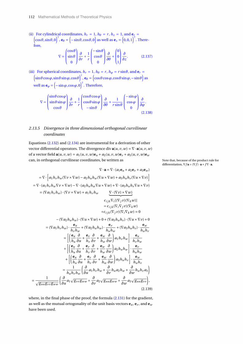
112 Mathematical Methods of Theoretical Physics

(ii) For cylindrical coordinates, hr = 1, hθ = r , hz = 1, and er =(cosθ, sinθ,0

)ᵀ, eθ =

(−sinθ,cosθ,0

)as well as ez =

(0,0,1

)ᵀ. There-

fore,

∇=

cosθ

sinθ

0

∂

∂r+ 1

r

−sinθ

cosθ

0

∂

∂θ+

0

0

1

∂

∂z. (2.137)

(iii) For spherical coordinates, hr = 1, hθ = r , hϕ = r sinθ, and er =(sinθcosϕ, sinθ sinϕ,cosθ

)ᵀ, eθ =

(cosθcosϕ,cosθ sinϕ,−sinθ

)as

well as eϕ =(−sinϕ,cosϕ,0

)ᵀ. Therefore,

∇=

sinθcosϕ

sinθ sinϕ

cosθ

∂

∂r+ 1

r

cosθcosϕ

cosθ sinϕ

−sinθ

∂

∂θ+ 1

r sinθ

−sinϕ

cosϕ

0

∂

∂ϕ.

(2.138)

2.13.5 Divergence in three dimensional orthogonal curvilinear

coordinates

Equations (2.132) and (2.134) are instrumental for a derivation of other

vector differential operators. The divergence div a(u, v , w) =∇·a(u, v , w)

of a vector field a(u, v , w) = a1(u, v , w)eu + a2(u, v , w)ev +a3(u, v , w)ew

can, in orthogonal curvilinear coordinates, be written as Note that, because of the product rule fordifferentiation, ∇ f a = (∇ f ) ·a+ f ∇·a.

∇·a =∇· (a1eu +a2ev +a3ew )

=∇·[

a1hv hw (∇v ×∇w)−a2huhw (∇u ×∇w)+a3huhv (∇u ×∇v)]

=∇· (a1hv hw∇v ×∇w)−∇· (a2huhw∇u ×∇w)+∇· (a3huhv∇u ×∇v)

= (∇a1hv hw ) · (∇v ×∇w)+a1hv hw ∇· (∇v)×∇w)︸ ︷︷ ︸εi j k∇i [(∇ j v)(∇k w)]

= εi j k (∇i∇ j v)(∇k w)

+εi j k (∇ j v)(∇i∇k w) = 0

− (∇a2huhw ) · (∇u ×∇w)+0+ (∇a3huhv ) · (∇u ×∇v)+0

= (∇a1hv hw ) · eu

hv hw+ (∇a2huhw ) · ev

huhw+ (∇a3huhv ) · ew

huhv

=[(

eu

hu

∂

∂u+ ev

hv

∂

∂v+ ew

hw

∂

∂w

)a1hv hw

]· eu

hv hw

+[(

eu

hu

∂

∂u+ ev

hv

∂

∂v+ ew

hw

∂

∂w

)a2huhw

]· ev

huhw

+[(

eu

hu

∂

∂u+ ev

hv

∂

∂v+ ew

hw

∂

∂w

)a3huhv

]· ew

huhv

= 1

huhv hw

(∂

∂ua1hv hw + ∂

∂vhu a2hw + ∂

∂whuhv a3

)= 1p

guu gv v gw w

(∂

∂ua1

pgv v gw w + ∂

∂va2

pguu gw w + ∂

∂wa3

pguu gv v

),

(2.139)

where, in the final phase of the proof, the formula (2.131) for the gradient,

as well as the mutual ortogonality of the unit basis vectors eu , ev , and ew

have been used.

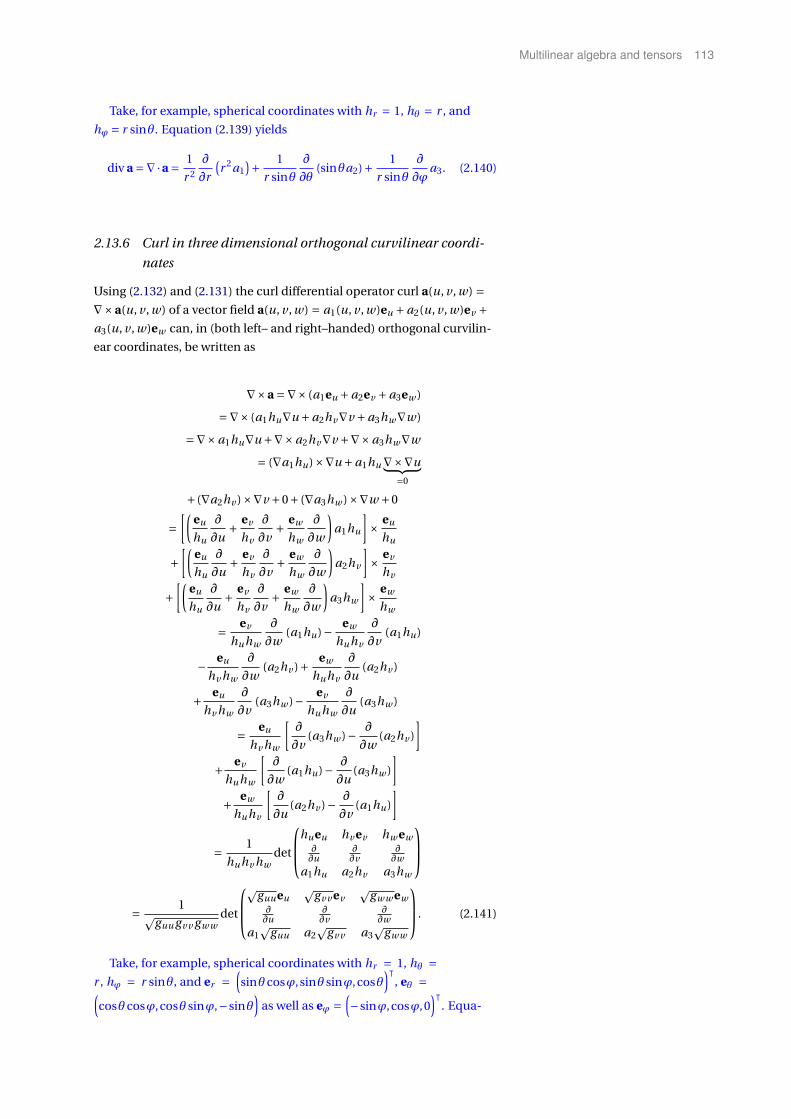
Multilinear algebra and tensors 113

Take, for example, spherical coordinates with hr = 1, hθ = r , and

hϕ = r sinθ. Equation (2.139) yields

div a =∇·a = 1

r 2

∂

∂r

(r 2a1

)+ 1

r sinθ

∂

∂θ(sinθa2)+ 1

r sinθ

∂

∂ϕa3. (2.140)

2.13.6 Curl in three dimensional orthogonal curvilinear coordi-

nates

Using (2.132) and (2.131) the curl differential operator curl a(u, v , w) =∇×a(u, v , w) of a vector field a(u, v , w) = a1(u, v , w)eu +a2(u, v , w)ev +a3(u, v , w)ew can, in (both left– and right–handed) orthogonal curvilin-

ear coordinates, be written as

∇×a =∇× (a1eu +a2ev +a3ew )

=∇× (a1hu∇u +a2hv∇v +a3hw∇w)

=∇×a1hu∇u +∇×a2hv∇v +∇×a3hw∇w

= (∇a1hu)×∇u +a1hu ∇×∇u︸ ︷︷ ︸=0

+ (∇a2hv )×∇v +0+ (∇a3hw )×∇w +0

=[(

eu

hu

∂

∂u+ ev

hv

∂

∂v+ ew

hw

∂

∂w

)a1hu

]× eu

hu

+[(

eu

hu

∂

∂u+ ev

hv

∂

∂v+ ew

hw

∂

∂w

)a2hv

]× ev

hv

+[(

eu

hu

∂

∂u+ ev

hv

∂

∂v+ ew

hw

∂

∂w

)a3hw

]× ew

hw

= ev

huhw

∂

∂w(a1hu)− ew

huhv

∂

∂v(a1hu)

− eu

hv hw

∂

∂w(a2hv )+ ew

huhv

∂

∂u(a2hv )

+ eu

hv hw

∂

∂v(a3hw )− ev

huhw

∂

∂u(a3hw )

= eu

hv hw

[∂

∂v(a3hw )− ∂

∂w(a2hv )

]+ ev

huhw

[∂

∂w(a1hu)− ∂

∂u(a3hw )

]+ ew

huhv

[∂

∂u(a2hv )− ∂

∂v(a1hu)

]

= 1

huhv hwdet

hu eu hv ev hw ew∂∂u

∂∂v

∂∂w

a1hu a2hv a3hw

= 1pguu gv v gw w

det

p

guu eup

gv v evp

gw w ew∂∂u

∂∂v

∂∂w

a1p

guu a2p

gv v a3p

gw w

. (2.141)

Take, for example, spherical coordinates with hr = 1, hθ =r , hϕ = r sinθ, and er =

(sinθcosϕ, sinθ sinϕ,cosθ

)ᵀ, eθ =(

cosθcosϕ,cosθ sinϕ,−sinθ)

as well as eϕ =(−sinϕ,cosϕ,0

)ᵀ. Equa-

114 Mathematical Methods of Theoretical Physics

tion (2.141) yields

rot a =∇×a = 1

r sinθ

sinθcosϕ

sinθ sinϕ

cosθ

(∂

∂θ(a3 sinθ)− ∂

∂ϕa2

)

+1

r

cosθcosϕ

cosθ sinϕ

−sinθ

(1

sinθ

∂

∂ϕa1 − ∂

∂r(r a3)

)+ 1

r

−sinϕ

cosϕ

0

(∂

∂r(r a2)− ∂

∂θa1

).

(2.142)

2.13.7 Laplacian in three dimensional orthogonal curvilinear

coordinates

Using (2.131) and (2.139) the second order Laplacian differential operator

∆a(u, v , w) = ∇ · [∇a(u, v , w)] of a field a(u, v , w) can, in orthogonal

curvilinear coordinates, be written as

∆a(u, v , w) =∇· [∇a(u, v , w)] =∇·(

eu

hu

∂

∂u+ ev

hv

∂

∂v+ ew

hw

∂

∂w

)a

= 1

huhv hw

[∂

∂u

hv hw

hu

∂

∂u+ ∂

∂v

huhw

hv

∂

∂v+ ∂

∂w

huhv

hw

∂

∂w

]a, (2.143)

so that the Lapace operator in orthogonal curvilinear coordinates can be

identified with

∆= 1

huhv hw

[∂

∂u

hv hw

hu

∂

∂u+ ∂

∂v

huhw

hv

∂

∂v+ ∂

∂w

huhv

hw

∂

∂w

]= 1p

guu gv v gw w

[∂

∂u

√gv v gw w

guu

∂

∂u+

+ ∂

∂v

√guu gw w

gv v

∂

∂v+ ∂

∂w

√guu gv v

gw w

∂

∂w

]

= 1pguu gv v gw w

∑t=u,v ,w

∂

∂t

pguu gv v gw w

g t t

∂

∂t. (2.144)

For the sake of examples, let us again consider cylindrical and spheri-

cal coordinates.

(i) The Laplace operator in cylindrical coordinates can be computed by

insertion of (2.128) hu = hr = 1, hv = hθ = r , and hw = hz = 1:

∆= 1

r

∂

∂rr sinθ

∂

∂r+ 1

r 2

∂2

∂θ2 + ∂2

∂ϕ2 . (2.145)

(ii) The Laplace operator in spherical coordinates can be computed by

insertion of (2.129) hu = hr = 1, hv = hθ = r , and hw = hϕ = r sinθ:

∆= 1

r 2

[∂

∂r

(r 2 ∂

∂r

)+ 1

sinθ

∂

∂θsinθ

∂

∂θ+ 1

sin2θ

∂2

∂ϕ2

]. (2.146)

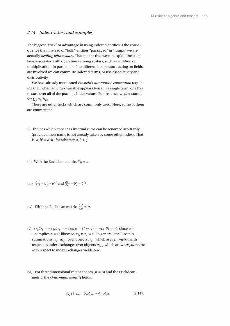
Multilinear algebra and tensors 115

2.14 Index trickery and examples

The biggest “trick” or advantage in using indexed entities is the conse-

quence that, instead of “bulk” entities “packaged” in “lumps” we are

actually dealing with scalars. That means that we can exploit the usual

laws associated with operations among scalars, such as addition or

multiplication. In particular, if no differential operators acting on fields

are involved we can commute indexed terms, or use associativity and

distributivity.

We have already mentioned Einstein’s summation convention requir-

ing that, when an index variable appears twice in a single term, one has

to sum over all of the possible index values. For instance, ai j b j k stands

for∑

j ai j b j k .

There are other tricks which are commonly used. Here, some of them

are enumerated:

(i) Indices which appear as internal sums can be renamed arbitrarily

(provided their name is not already taken by some other index). That

is, ai bi = a j b j for arbitrary a,b, i , j .

(ii) With the Euclidean metric, δi i = n.

(iii) ∂xi

∂x j = δij = δi j and ∂xi

∂x j= δ j

i = δi j .

(iv) With the Euclidean metric, ∂xi

∂xi = n.

(v) εi jδi j = −ε j iδi j = −ε j iδ j i = (i ↔ j ) = −εi jδi j = 0, since a =−a implies a = 0; likewise, εi j xi x j = 0. In general, the Einstein

summations si j ...ai j ... over objects si j ... which are symmetric with

respect to index exchanges over objects ai j ... which are antisymmetric

with respect to index exchanges yields zero.

(vi) For threedimensional vector spaces (n = 3) and the Euclidean

metric, the Grassmann identity holds:

εi j kεklm = δi lδ j m −δi mδ j l . (2.147)

116 Mathematical Methods of Theoretical Physics

For the sake of a proof, consider

x× (y×z) ≡in index notation

x jεi j k yl zmεklm = x j yl zmεi j kεklm ≡in coordinate notationx1

x2

x3

×

y1

y2

y3

×

z1

z2

z3

=

x1

x2

x3

×

y2z3 − y3z2

y3z1 − y1z3

y1z2 − y2z1

=

x2(y1z2 − y2z1)−x3(y3z1 − y1z3)

x3(y2z3 − y3z2)−x1(y1z2 − y2z1)

x1(y3z1 − y1z3)−x2(y2z3 − y3z2)

=

x2 y1z2 −x2 y2z1 −x3 y3z1 +x3 y1z3

x3 y2z3 −x3 y3z2 −x1 y1z2 +x1 y2z1

x1 y3z1 −x1 y1z3 −x2 y2z3 +x2 y3z2

=

y1(x2z2 +x3z3)− z1(x2 y2 +x3 y3)

y2(x3z3 +x1z1)− z2(x1 y1 +x3 y3)

y3(x1z1 +x2z2)− z3(x1 y1 +x2 y2)

(2.148)

The “incomplete” dot products can be completed through addition

and subtraction of the same term, respectively; that is,y1(x1z1 +x2z2 +x3z3)− z1(x1 y1 +x2 y2 +x3 y3)

y2(x1z1 +x2z2 +x3z3)− z2(x1 y1 +x2 y2 +x3 y3)

y3(x1z1 +x2z2 +x3z3)− z3(x1 y1 +x2 y2 +x3 y3)

≡ in vector notation

y (x ·z)−z(x ·y

)≡ in index notation

x j yl zm(δi lδ j m −δi mδ j l

). (2.149)

(vii) For threedimensional vector spaces (n = 3) and the Euclidean

metric the Grassmann identity (2.147) implies

‖a ×b‖ =√εi j kεi st a j as bk bt =

√‖a‖2‖b‖2 − (a ·b)2

=√√√√det

(a ·a a ·b

a ·b b ·b

)=

√‖a‖2‖b‖2

(1−cos2∠ab

)= ‖a‖‖b‖sin∠ab .

(2.150)

(viii) Let u, v ≡ x ′1, x ′

2 be two parameters associated with an orthonormal

Cartesian basis (0,1), (1,0), and letΦ : (u, v) 7→R3 be a mapping from

some area of R2 into a twodimensional surface of R3. Then the metric

tensor is given by gi j = ∂Φk

∂y i∂Φm

∂y j δkm .

Consider the following examples in three-dimensional vector space.

Let r 2 =∑3i=1 x2

i .

Multilinear algebra and tensors 117

1.

∂ j r = ∂ j

√∑i

x2i = 1

2

1√∑i x2

i

2x j =x j

r(2.151)

By using the chain rule one obtains

∂ j rα =αrα−1 (∂ j r

)=αrα−1( x j

r

)=αrα−2x j (2.152)

and thus ∇rα =αrα−2x.

2.

∂ j logr = 1

r

(∂ j r

)(2.153)

With ∂ j r = x j

r derived earlier in Equation (2.152) one obtains ∂ j logr =1r

x j

r = x j

r 2 , and thus ∇ logr = xr 2 .

3.

∂ j

(∑i

(xi −ai )2

)− 12

+(∑

i(xi +ai )2

)− 12

=

=−1

2

1(∑i (xi −ai )2

) 32

2(x j −a j

)+ 1(∑i (xi +ai )2

) 32

2(x j +a j

)=−

(∑i

(xi −ai )2

)− 32 (

x j −a j)−(∑

i(xi +ai )2

)− 32 (

x j +a j)

.

(2.154)

4. For three dimensions and for r 6= 0,

∇( r

r 3

)≡ ∂i

( ri

r 3

)= 1

r 3 ∂i ri︸︷︷︸=3

+ri

(−3

1

r 4

)(1

2r

)2ri = 3

1

r 3 −31

r 3 = 0. (2.155)

5. With this solution (2.155) one obtains, for three dimensions and r 6= 0,

∆(1

r

)≡ ∂i∂i1

r= ∂i

(− 1

r 2

)(1

2r

)2ri =−∂i

ri

r 3 = 0. (2.156)

6. With the earlier solution (2.155) one obtains

∆(rp

r 3

)≡ ∂i∂ir j p j

r 3 = ∂i

[pi

r 3 + r j p j

(−3

1

r 5

)ri

]= pi

(−3

1

r 5

)ri +pi

(−3

1

r 5

)ri

+r j p j

[(15

1

r 6

)(1

2r

)2ri

]ri + r j p j

(−3

1

r 5

)∂i ri︸︷︷︸=3

= ri pi1

r 5 (−3−3+15−9) = 0 (2.157)

7. With r 6= 0 and constant p one obtains

Note that, in three dimensions, theGrassmann identity (2.147) εi j kεklm =δi lδ j m −δi mδ j l holds.

118 Mathematical Methods of Theoretical Physics

∇× (p× r

r 3 ) ≡ εi j k∂ jεklm plrm

r 3 = plεi j kεklm

[∂ j

rm

r 3

]= plεi j kεklm

[1

r 3 ∂ j rm + rm

(−3

1

r 4

)(1

2r

)2r j

]= plεi j kεklm

[1

r 3 δ j m −3r j rm

r 5

]= pl (δi lδ j m −δi mδ j l )

[1

r 3 δ j m −3r j rm

r 5

]= pi

(3

1

r 3 −31

r 3

)︸ ︷︷ ︸

=0

−p j

(1

r 3 ∂ j ri︸︷︷︸=δi j

−3r j ri

r 5

)

=− p

r 3 +3

(rp

)r

r 5 . (2.158)

8.

∇× (∇Φ)

≡ εi j k∂ j∂kΦ

= εi k j∂k∂ jΦ

= εi k j∂ j∂kΦ

=−εi j k∂ j∂kΦ= 0. (2.159)

This is due to the fact that ∂ j∂k is symmetric, whereas εi j k is totally

antisymmetric.

9. For a proof of (x×y)×z 6= x× (y×z) consider

(x×y)×z

≡ εi j m︸︷︷︸second ×

ε j kl︸︷︷︸first ×

xk yl zm

=−εi m jε j kl xk yl zm

=−(δi kδml −δi mδlk )xk yl zm

=−xi y ·z+ yi x ·z. (2.160)

versus

x× (y×z)

≡ εi k j︸︷︷︸first ×

ε j l m︸︷︷︸second ×

xk yl zm

= (δi lδkm −δi mδkl )xk yl zm

= yi x ·z− zi x ·y. (2.161)

10. Let w = pr with pi = pi

(t − r

c

), whereby t and c are constants. Then,

divw = ∇·w

≡ ∂i wi = ∂i

[1

rpi

(t − r

c

)]=

=(− 1

r 2

)(1

2r

)2ri pi + 1

rp ′

i

(−1

c

)(1

2r

)2ri

= − ri pi

r 3 − 1

cr 2 p ′i ri .

Hence, divw =∇·w =−(

rpr 3 + rp′

cr 2

).

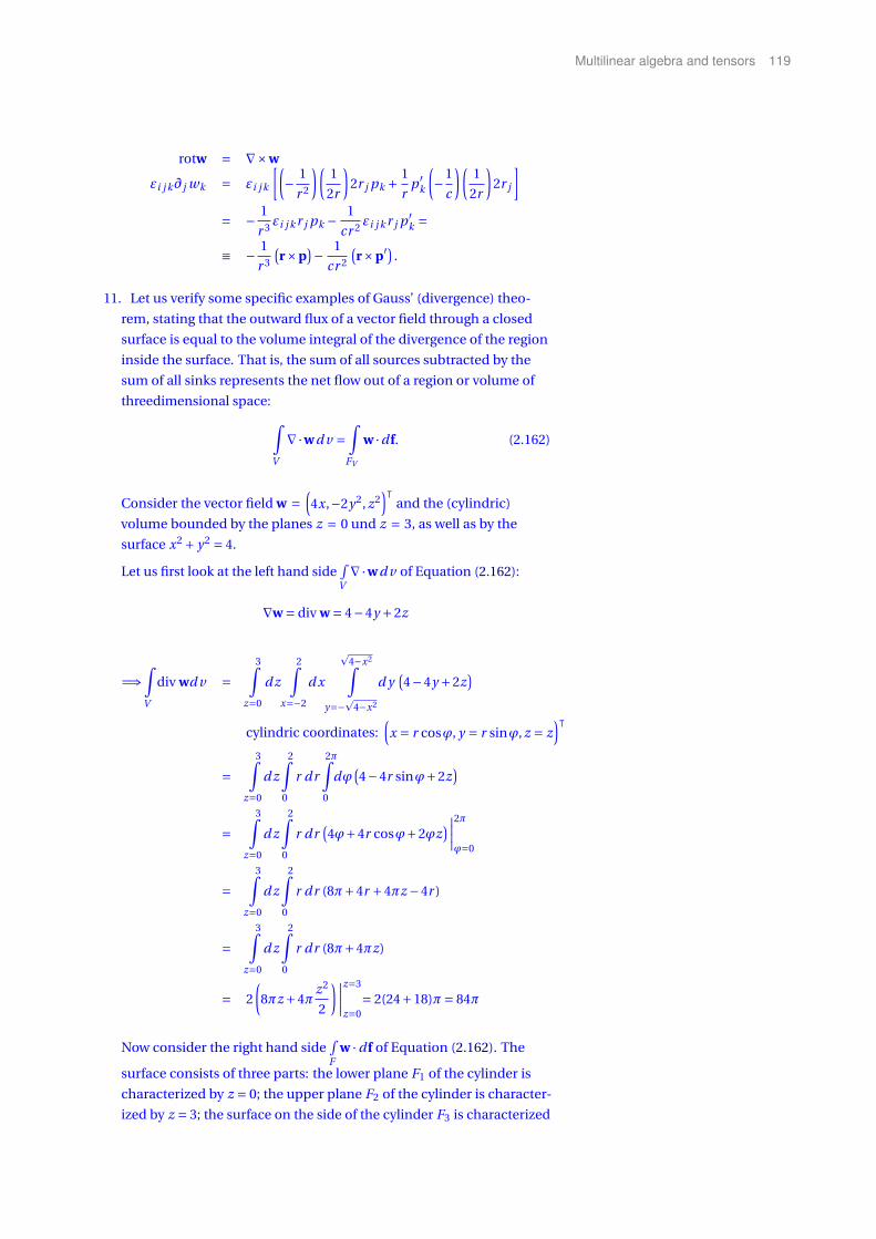
Multilinear algebra and tensors 119

rotw = ∇×w

εi j k∂ j wk = εi j k

[(− 1

r 2

)(1

2r

)2r j pk +

1

rp ′

k

(−1

c

)(1

2r

)2r j

]= − 1

r 3 εi j k r j pk −1

cr 2 εi j k r j p ′k =

≡ − 1

r 3

(r×p

)− 1

cr 2

(r×p′) .

11. Let us verify some specific examples of Gauss’ (divergence) theo-

rem, stating that the outward flux of a vector field through a closed

surface is equal to the volume integral of the divergence of the region

inside the surface. That is, the sum of all sources subtracted by the

sum of all sinks represents the net flow out of a region or volume of

threedimensional space: ∫V

∇·wd v =∫

FV

w ·df. (2.162)

Consider the vector field w =(4x,−2y2, z2

)ᵀand the (cylindric)

volume bounded by the planes z = 0 und z = 3, as well as by the

surface x2 + y2 = 4.

Let us first look at the left hand side∫V∇·wd v of Equation (2.162):

∇w = div w = 4−4y +2z

=⇒∫V

div wd v =3∫

z=0

d z

2∫x=−2

d x

p4−x2∫

y=−p

4−x2

d y(4−4y +2z

)cylindric coordinates:

(x = r cosϕ, y = r sinϕ, z = z

)ᵀ=

3∫z=0

d z

2∫0

r dr

2π∫0

dϕ(4−4r sinϕ+2z

)

=3∫

z=0

d z

2∫0

r dr(4ϕ+4r cosϕ+2ϕz

)∣∣∣∣2π

ϕ=0

=3∫

z=0

d z

2∫0

r dr (8π+4r +4πz −4r )

=3∫

z=0

d z

2∫0

r dr (8π+4πz)

= 2

(8πz +4π

z2

2

)∣∣∣∣z=3

z=0= 2(24+18)π= 84π

Now consider the right hand side∫F

w ·df of Equation (2.162). The

surface consists of three parts: the lower plane F1 of the cylinder is

characterized by z = 0; the upper plane F2 of the cylinder is character-

ized by z = 3; the surface on the side of the cylinder F3 is characterized

120 Mathematical Methods of Theoretical Physics

by x2 + y2 = 4. df must be normal to these surfaces, pointing outwards;

hence (since the area of a circle of radius r = 2 is πr 2 = 4π),

F1 :∫

F1

w ·df1 =∫

F1

4x

−2y2

z2 = 0

0

0

−1

d xd y = 0

F2 :∫

F2

w ·df2 =∫

F2

4x

−2y2

z2 = 9

0

0

1

d xd y

= 9∫

Kr=2

d f = 9 ·4π= 36π

F3 :∫

F3

w ·df3 =∫

F3

4x

−2y2

z2

(∂x

∂ϕ× ∂x

∂z

)dϕd z (r = 2)

∂x

∂ϕ=

−r sinϕ

r cosϕ

0

=

−2sinϕ

2cosϕ

0

;∂x

∂z=

0

0

1

,

and therefore

∂x

∂ϕ× ∂x

∂z=

2cosϕ

2sinϕ

0

,

and

F3 =2π∫

ϕ=0

dϕ

3∫z=0

d z

4 ·2cosϕ

−2(2sinϕ)2

z2

2cosϕ

2sinϕ

0

=

2π∫ϕ=0

dϕ

3∫z=0

d z(16cos2ϕ−16sin3ϕ

)

= 3 ·16

2π∫ϕ=0

dϕ(cos2ϕ− sin3ϕ

)

=[ ∫

cos2ϕdϕ = ϕ2 + 1

4 sin2ϕ∫sin3ϕdϕ = −cosϕ+ 1

3 cos3ϕ

]

= 3 ·16

2π

2−

[(1+ 1

3

)−

(1+ 1

3

)]︸ ︷︷ ︸

=0

= 48π

For the flux through the surfaces one thus obtains∮F

w ·df = F1 +F2 +F3 = 84π.

12. Let us verify some specific examples of Stokes’ theorem in three

dimensions, stating that∫F

rot b ·df =∮

CF

b ·ds. (2.163)

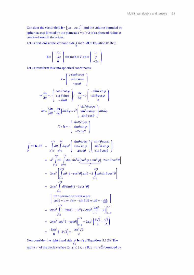
Multilinear algebra and tensors 121

Consider the vector field b =(

y z,−xz,0)ᵀ

and the volume bounded by

spherical cap formed by the plane at z = a/p

2 of a sphere of radius a

centered around the origin.

Let us first look at the left hand side∫F

rot b ·df of Equation (2.163):

b =

y z

−xz

0

=⇒ rot b =∇×b =

x

y

−2z

Let us transform this into spherical coordinates:

x =

r sinθcosϕ

r sinθ sinϕ

r cosθ

⇒ ∂x

∂θ= r

cosθcosϕ

cosθ sinϕ

−sinθ

;∂x

∂ϕ= r

−sinθ sinϕ

sinθcosϕ

0

df =(∂x

∂θ× ∂x

∂ϕ

)dθdϕ= r 2

sin2θcosϕ

sin2θ sinϕ

sinθcosθ

dθdϕ

∇×b = r

sinθcosϕ

sinθ sinϕ

−2cosθ

∫F

rot b ·df =π/4∫

θ=0

dθ

2π∫ϕ=0

dϕa3

sinθcosϕ

sinθ sinϕ

−2cosθ

sin2θcosϕ

sin2θ sinϕ

sinθcosθ

= a3

π/4∫θ=0

dθ

2π∫ϕ=0

dϕ

[sin3θ

(cos2ϕ+ sin2ϕ

)︸ ︷︷ ︸=1

−2sinθcos2θ

]

= 2πa3

π/4∫θ=0

dθ(1−cos2θ

)sinθ−2

π/4∫θ=0

dθ sinθcos2θ

= 2πa3

π/4∫θ=0

dθ sinθ(1−3cos2θ

)[

transformation of variables:

cosθ = u ⇒ du =−sinθdθ⇒ dθ =− dusinθ

]

= 2πa3

π/4∫θ=0

(−du)(1−3u2)= 2πa3

(3u3

3−u

)∣∣∣∣π/4

θ=0

= 2πa3 (cos3θ−cosθ

)∣∣∣∣π/4

θ=0= 2πa3

(2p

2

8−p

2

2

)

= 2πa3

8

(−2

p2)=−πa3

p2

2

Now consider the right hand side∮

CF

b ·ds of Equation (2.163). The

radius r ′ of the circle surface (x, y , z) | x, y ∈ R, z = a/p

2 bounded by

122 Mathematical Methods of Theoretical Physics

the sphere with radius a is determined by a2 = (r ′)2 + (a/p

2)2; hence,

r ′ = a/p

2. The curve of integration CF can be parameterized by

(x, y , z) | x = ap2

cosϕ, y = ap2

sinϕ, z = ap2

.

Therefore,

x = a

1p2

cosϕ

1p2

sinϕ

1p2

= ap2

cosϕ

sinϕ

1

∈CF

Let us transform this into polar coordinates:

ds = dx

dϕdϕ= ap

2

−sinϕ

cosϕ

0

dϕ

b =

ap2

sinϕ · ap2

− ap2

cosϕ · ap2

0

= a2

2

sinϕ

−cosϕ

0

Hence the circular integral is given by

∮CF

b ·ds = a2

2

ap2

2π∫ϕ=0

(−sin2ϕ−cos2ϕ)︸ ︷︷ ︸

=−1

dϕ=− a3

2p

22π=−a3πp

2.

13. In machine learning, a linear regression Ansatz5 is to find a linear 5 Ian Goodfellow, Yoshua Bengio, andAaron Courville. Deep Learning. MIT Press,Cambridge, MA, November 2016. ISBN9780262035613, 9780262337434. URLhttps://mitpress.mit.edu/books/

deep-learning

model for the prediction of some unknown observable, given some

anecdotal instances of its performance. More formally, let y be an

arbitrary real-valued observable which depends on n real-valued

parameters x1, . . . , xn by linear means; that is, by

y =n∑

i=1xi ri = ⟨x|r⟩, (2.164)

where ⟨x| = (|x⟩)ᵀ is the transpose of the vector |x⟩. The tuple

|r⟩ =(r1, . . . ,rn

)ᵀ(2.165)

contains the unknown weights of the approximation – the “theory,” if

you like – and ⟨a|b⟩ =∑i ai bi stands for the Euclidean scalar product

of the tuples interpreted as (dual) vectors in n-dimensional (dual)

vector space Rn .

Given are m known instances of (2.164); that is, suppose m real-valued

pairs(z j , |x j ⟩

)are known. These data can be bundled into an m-tuple

|z⟩ ≡(z j1 , . . . , z jm

)ᵀ, (2.166)

and an (m ×n)-matrix

X≡

x j1i1 . . . x j1in

......

...

x jm i1 . . . x jm in

(2.167)

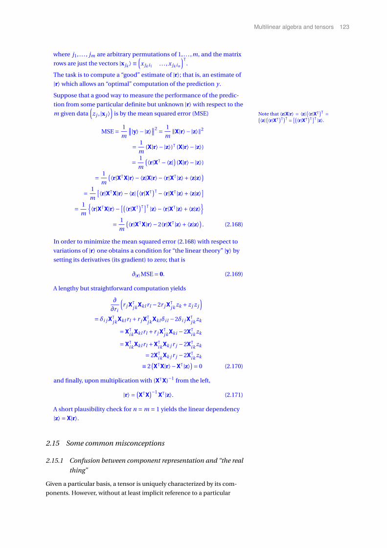
Multilinear algebra and tensors 123

where j1, . . . , jm are arbitrary permutations of 1, . . . ,m, and the matrix

rows are just the vectors |x jk ⟩ ≡(x jk i1 . . . , x jk in

)ᵀ.

The task is to compute a “good” estimate of |r⟩; that is, an estimate of

|r⟩ which allows an “optimal” computation of the prediction y .

Suppose that a good way to measure the performance of the predic-

tion from some particular definite but unknown |r⟩ with respect to the

m given data(z j , |x j ⟩

)is by the mean squared error (MSE) Note that ⟨z|X|r⟩ = ⟨z|(⟨r|Xᵀ)ᵀ =(⟨z|(⟨r|Xᵀ)ᵀ)ᵀ = [(⟨r|Xᵀ)ᵀ]ᵀ |z⟩.

MSE = 1

m

∥∥|y⟩− |z⟩∥∥2 = 1

m‖X|r⟩− |z⟩‖2

= 1

m(X|r⟩− |z⟩)ᵀ (X|r⟩− |z⟩)

= 1

m

(⟨r|Xᵀ−⟨z|) (X|r⟩− |z⟩)

= 1

m

(⟨r|XᵀX|r⟩−⟨z|X|r⟩−⟨r|Xᵀ|z⟩+⟨z|z⟩)= 1

m

[⟨r|XᵀX|r⟩−⟨z|(⟨r|Xᵀ)ᵀ−⟨r|Xᵀ|z⟩+⟨z|z⟩]= 1

m

⟨r|XᵀX|r⟩− [(⟨r|Xᵀ)ᵀ]ᵀ |z⟩−⟨r|Xᵀ|z⟩+⟨z|z⟩

= 1

m

(⟨r|XᵀX|r⟩−2⟨r|Xᵀ|z⟩+⟨z|z⟩) . (2.168)

In order to minimize the mean squared error (2.168) with respect to

variations of |r⟩ one obtains a condition for “the linear theory” |y⟩ by

setting its derivatives (its gradient) to zero; that is

∂|r⟩MSE = 0. (2.169)

A lengthy but straightforward computation yields

∂

∂ri

(r j Xᵀ

j k Xkl rl −2r j Xᵀj k zk + z j z j

)= δi j Xᵀ

j k Xkl rl + r j Xᵀj k Xklδi l −2δi j Xᵀ

j k zk

=Xᵀi k Xkl rl + r j Xᵀ

j k Xki −2Xᵀi k zk

=Xᵀi k Xkl rl +Xᵀ

i k Xk j r j −2Xᵀi k zk

= 2Xᵀi k Xk j r j −2Xᵀ

i k zk

≡ 2(XᵀX|r⟩−Xᵀ|z⟩)= 0 (2.170)

and finally, upon multiplication with (XᵀX)−1 from the left,

|r⟩ = (XᵀX

)−1 Xᵀ|z⟩. (2.171)

A short plausibility check for n = m = 1 yields the linear dependency

|z⟩ =X|r⟩.

2.15 Some common misconceptions

2.15.1 Confusion between component representation and “the real

thing”

Given a particular basis, a tensor is uniquely characterized by its com-

ponents. However, without at least implicit reference to a particular

124 Mathematical Methods of Theoretical Physics

basis, the enumeration of components of tuples are just blurbs, and such

“tensors” remain undefined.

Example (wrong!): a type-1 tensor (i.e., a vector) is given by (1,2)ᵀ.

Correct: with respect (relative) to the basis (0,1)ᵀ, (1,0)ᵀ, a (rank,

degree, order) type-1 tensor (a vector) is given by (1,2)ᵀ.

2.15.2 Matrix as a representation of a tensor of type (order, degree,

rank) two

A matrix “is” not a tensor; but a tensor of type (order, degree, rank) 2 can

be represented or encoded as a matrix with respect (relative) to some ba-

sis. Example (wrong!): A matrix is a tensor of type (or order, degree, rank)

2. Correct: with respect to the basis (0,1)ᵀ, (1,0)ᵀ, a matrix represents a

type-2 tensor. The matrix components are the tensor components.

Also, for non-orthogonal bases, covariant, contravariant, and mixed

tensors correspond to different matrices.

c

Groups as permutations 125

3Groups as permutations

G RO U P T H E O RY is about transformations, actions, and the symmetries

presenting themselves in terms of invariants with respect to those trans-

formations and actions. One of the central axioms is the reversibility – in

mathematical terms, the invertibility – of all operations: every transfor-

mation has a unique inverse transformation. Another one is associativity;

that is, the property that the order of the transformations is irrelevant.

These properties have far-reaching implications: from a functional per-

spective, group theory amounts to the study of permutations among the

sets involved; nothing more and nothing less.

Rather than citing standard texts on group theory1 the reader is 1 Joseph J. Rotman. An Introductionto the Theory of Groups, volume 148 ofGraduate texts in mathematics. Springer,New York, fourth edition, 1995. ISBN978-0-387-94285-8,978-1-4612-8686-8,978-1-4612-4176-8. D O I : 10.1007/978-1-4612-4176-8. URL https://doi.org/10.

1007/978-1-4612-4176-8

encouraged to consult two internet resources: Dimitri Vvedensky’s group

theory course notes,2 as well as John Eliott’s youtube presentation3 for

2 Dimitry D. Vvedensky. Group theory,2001. URL http://www.cmth.ph.ic.ac.

uk/people/d.vvedensky/courses.html.accessed on March 12th, 20183 John Eliott. Group theory, 2015. URLhttps://youtu.be/O4plQ5ppg9c?list=

PLAvgI3H-gclb_Xy7eTIXkkKt3KlV6gk9_.accessed on March 12th, 2018

an online course on group theory. Hall’s introductions to Lie groups4

4 Brian C. Hall. An elementaryintroduction to groups and rep-resentations, 2000. URL https:

//arxiv.org/abs/math-ph/0005032;and Brian C. Hall. Lie Groups, Lie Algebras,and Representations. An ElementaryIntroduction, volume 222 of GraduateTexts in Mathematics. Springer Interna-tional Publishing, Cham, Heidelberg, NewYork, Dordrecht, London, second edition,2003,2015. ISBN 978-3-319-13466-6,978-3-319-37433-8. D O I : 10.1007/978-3-319-13467-3. URL https://doi.org/10.

1007/978-3-319-13467-3

contain fine presentations thereof.

3.1 Basic definition and properties

3.1.1 Group axioms

A group is a set of objects G which satisfy the following conditions (or,

stated differently, axioms):

(i) closure: There exists a map, or composition rule : G ×G →G , from

G ×G into G which is closed under any composition of elements;

that is, the combination a b of any two elements a,b ∈ G results

in an element of the group G . That is, the composition never yields

anything “outside” of the group;

(ii) associativity: for all a, b, and c in G , the following equality holds:

a (b c) = (a b) c. Associativity amounts to the requirement that

the order of the operations is irrelevant, thereby restricting group

operations to permutations;

(iii) identity (element): there exists an element of G , called the identity

(element) and denoted by I , such that for all a in G , a I = I a = a.

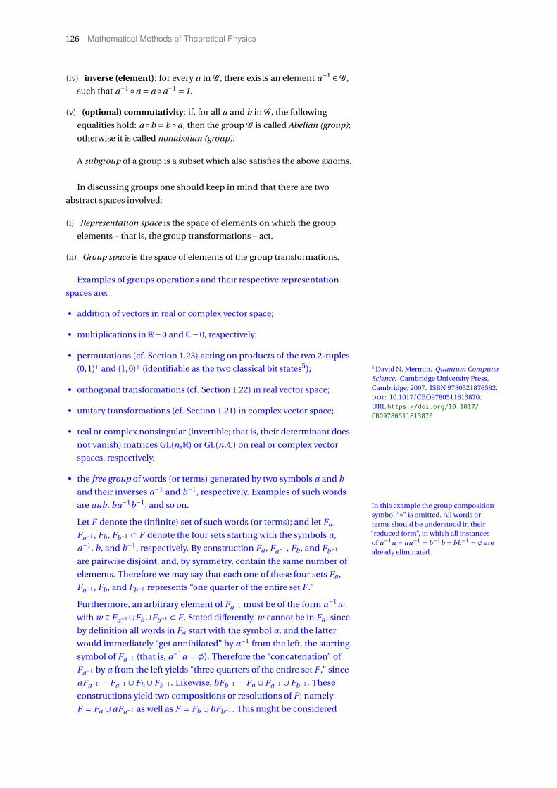
126 Mathematical Methods of Theoretical Physics

(iv) inverse (element): for every a in G , there exists an element a−1 ∈G ,

such that a−1 a = a a−1 = I .

(v) (optional) commutativity: if, for all a and b in G , the following

equalities hold: a b = b a, then the group G is called Abelian (group);

otherwise it is called nonabelian (group).

A subgroup of a group is a subset which also satisfies the above axioms.

In discussing groups one should keep in mind that there are two

abstract spaces involved:

(i) Representation space is the space of elements on which the group

elements – that is, the group transformations – act.

(ii) Group space is the space of elements of the group transformations.

Examples of groups operations and their respective representation

spaces are:

• addition of vectors in real or complex vector space;

• multiplications in R−0 and C−0, respectively;

• permutations (cf. Section 1.23) acting on products of the two 2-tuples

(0,1)ᵀ and (1,0)ᵀ (identifiable as the two classical bit states5); 5 David N. Mermin. Quantum ComputerScience. Cambridge University Press,Cambridge, 2007. ISBN 9780521876582.D O I : 10.1017/CBO9780511813870.URL https://doi.org/10.1017/

CBO9780511813870

• orthogonal transformations (cf. Section 1.22) in real vector space;

• unitary transformations (cf. Section 1.21) in complex vector space;

• real or complex nonsingular (invertible; that is, their determinant does

not vanish) matrices GL(n,R) or GL(n,C) on real or complex vector

spaces, respectively.

• the free group of words (or terms) generated by two symbols a and b

and their inverses a−1 and b−1, respectively. Examples of such words

are aab, ba−1b−1, and so on. In this example the group compositionsymbol “” is omitted. All words orterms should be understood in their“reduced form”, in which all instancesof a−1a = aa−1 = b−1b = bb−1 = ; arealready eliminated.

Let F denote the (infinite) set of such words (or terms); and let Fa ,

Fa−1 , Fb , Fb−1 ⊂ F denote the four sets starting with the symbols a,

a−1, b, and b−1, respectively. By construction Fa , Fa−1 , Fb , and Fb−1

are pairwise disjoint, and, by symmetry, contain the same number of

elements. Therefore we may say that each one of these four sets Fa ,

Fa−1 , Fb , and Fb−1 represents “one quarter of the entire set F .”

Furthermore, an arbitrary element of Fa−1 must be of the form a−1w ,

with w ∈ Fa−1∪Fb∪Fb−1 ⊂ F . Stated differently, w cannot be in Fa , since

by definition all words in Fa start with the symbol a, and the latter

would immediately “get annihilated” by a−1 from the left, the starting

symbol of Fa−1 (that is, a−1a = ;). Therefore the “concatenation” of

Fa−1 by a from the left yields “three quarters of the entire set F ,” since

aFa−1 = Fa−1 ∪Fb ∪Fb−1 . Likewise, bFb−1 = Fa ∪Fa−1 ∪Fb−1 . These

constructions yield two compositions or resolutions of F ; namely

F = Fa ∪ aFa−1 as well as F = Fb ∪bFb−1 . This might be considered

Groups as permutations 127

“paradoxical” because, at the same time, F = Fa ∪Fa−1 ∪Fb ∪Fb−1 ; with These constructions are rooted in“paradoxes of infinity,” such as Hilbert’shotel.

pairwise disjoint Fa , Fa−1 , Fb , and Fb−1 .

We may identify the two words with different rotations (of a certain

notrivial, independent, kind6) of points on the sphere. This can be 6 F. Hausdorff. Bemerkung über denInhalt von Punktmengen. MathematischeAnnalen, 75(3):428–433, Sep 1914. ISSN1432-1807. D O I : 10.1007/BF01563735.URL https://doi.org/10.1007/

BF01563735

applied to the parametrization of a sphere giving rise to the Banach-

Tarski paradox.7

7 Stan Wagon. The Banach-Tarski Para-dox. Encyclopedia of Mathematicsand its Applications. Cambridge Uni-versity Press, Cambridge, 1985. D O I :10.1017/CBO9780511609596. URL https:

//doi.org/10.1017/CBO9780511609596

3.1.2 Discrete and continuous groups

The order |G | of a group G is the number of distinct elements of that

group. If the order is finite or denumerable, the group is called discrete. If

the group contains a continuity of elements, the group is called continu-

ous.

A continuous group can geometrically be imagined as a linear space

(e.g., a linear vector or matrix space) in which every point in this linear

space is an element of that group.

3.1.3 Generators and relations in finite groups

The following notation will be used: an = a · · · a︸ ︷︷ ︸n times

.

Elements of finite groups eventually “cycle back;” that is, multiple (but

finite) operations of the same arbitrary element a ∈ G will eventually

yield the identity: a · · · a︸ ︷︷ ︸k times

= ak = I . The period of a ∈ G is defined by

e, a1, a2, . . . , ak−1.

A generating set of a group is a minimal subset – a “basis” of sorts – of

that group such that every element of the group can be expressed as the

composition of elements of this subset and their inverses. Elements of

the generating set are called generators. These independent elements

form a basis for all group elements. The dimension of a group is the

number of independent transformations of that group, which is the

number of elements in a generating set. The coordinates are defined

relative to (in terms of) the basis elements.

Relations are equations in those generators which hold for the group

so that all other equations which hold for the group can be derived from

those relations.

3.1.4 Uniqueness of identity and inverses

One important consequence of the axioms is the uniqueness of the

identity and the inverse elements. In a proof by contradiction of the

uniqueness of the identity, suppose that I is not unique; that is, there

would exist (at least) two identity elements I , I ′ ∈G with I 6= I ′ such that

I a = I ′ a = a. This assumption yields a complete contradiction, since

right composition with the inverse a−1 of a, together with associativity,

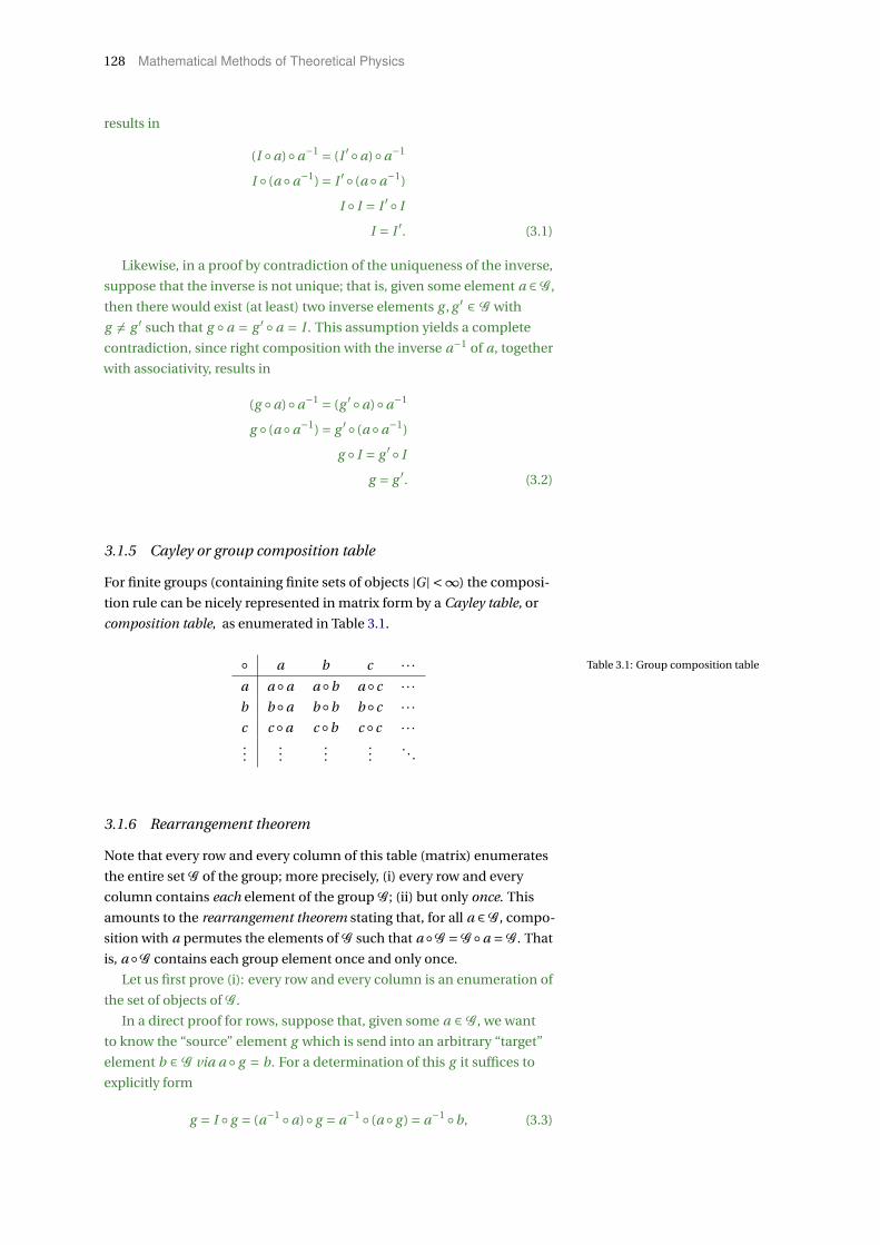
128 Mathematical Methods of Theoretical Physics

results in

(I a)a−1 = (I ′ a)a−1

I (a a−1) = I ′ (a a−1)

I I = I ′ I

I = I ′. (3.1)

Likewise, in a proof by contradiction of the uniqueness of the inverse,

suppose that the inverse is not unique; that is, given some element a ∈G ,

then there would exist (at least) two inverse elements g , g ′ ∈ G with

g 6= g ′ such that g a = g ′ a = I . This assumption yields a complete

contradiction, since right composition with the inverse a−1 of a, together

with associativity, results in

(g a)a−1 = (g ′ a)a−1

g (a a−1) = g ′ (a a−1)

g I = g ′ I

g = g ′. (3.2)

3.1.5 Cayley or group composition table

For finite groups (containing finite sets of objects |G| <∞) the composi-

tion rule can be nicely represented in matrix form by a Cayley table, or

composition table, as enumerated in Table 3.1.

a b c · · ·a a a a b a c · · ·b b a b b b c · · ·c c a c b c c · · ·...

......

.... . .

Table 3.1: Group composition table

3.1.6 Rearrangement theorem

Note that every row and every column of this table (matrix) enumerates

the entire set G of the group; more precisely, (i) every row and every

column contains each element of the group G ; (ii) but only once. This

amounts to the rearrangement theorem stating that, for all a ∈G , compo-

sition with a permutes the elements of G such that a G =G a =G . That

is, a G contains each group element once and only once.

Let us first prove (i): every row and every column is an enumeration of

the set of objects of G .

In a direct proof for rows, suppose that, given some a ∈ G , we want

to know the “source” element g which is send into an arbitrary “target”

element b ∈ G via a g = b. For a determination of this g it suffices to

explicitly form

g = I g = (a−1 a) g = a−1 (a g ) = a−1 b, (3.3)

Groups as permutations 129

which is the element “sending a, if multiplied from the right hand side

(with respect to a), into b.”

Likewise, in a direct proof for columns, suppose that, given some

a ∈ G , we want to know the “source” element g which is send into an

arbitrary “target” element b ∈G via g a = b. For a determination of this g

it suffices to explicitly form

g = g I = g (a a−1) = (g a)a−1 = b a−1, (3.4)

which is the element “sending a, if multiplied from the left hand side

(with respect to a), into b.”

Uniqueness (ii) can be proven by complete contradiction: suppose

there exists a row with two identical entries a at different places, “coming

(via a single c depending on the row) from different sources b and b′;”that is, c b = c b′ = a, with b 6= b′. But then, left composition with c−1,

together with associativity, yields

c−1 (c b) = c−1 (c b′)

(c−1 c)b = (c−1 c)b′

I b = I b′

b = b′. (3.5)

Likewise, suppose there exists a column with two identical entries a at

different places, “coming (via a single c depending on the column) from

different sources b and b′;” that is, b c = b′ c = a, with b 6= b′. But then,

right composition with c−1, together with associativity, yields

(b c) c−1 = (b′ c) c−1

b (c c−1) = b′ (c c−1)

b I = b′ I

b = b′. (3.6)

Exhaustion (i) and uniqueness (ii) impose rather stringent conditions

on the composition rules, which essentially have to permute elements of

the set of the group G . Syntactically, simultaneously every row and every

column of a matrix representation of some group composition table must

contain the entire set G .

Note also that Abelian groups have composition tables which are

symmetric along its diagonal axis; that is, they are identical to their

transpose. This is a direct consequence of the Abelian property a b = b a.

3.2 Zoology of finite groups up to order 6

To give a taste of group zoology there is only one group of order 2, 3 and 5;

all three are Abelian. One (out of two groups) of order 6 is nonabelian. http://www.math.niu.edu/

~beachy/aaol/grouptables1.

html, accessed on March 14th,

2018.3.2.1 Group of order 2

Table 3.2 enumerates all 24 binary functions of two bits; only the two

mappings represented by Tables 3.2(7) and 3.2(10) represent groups, with

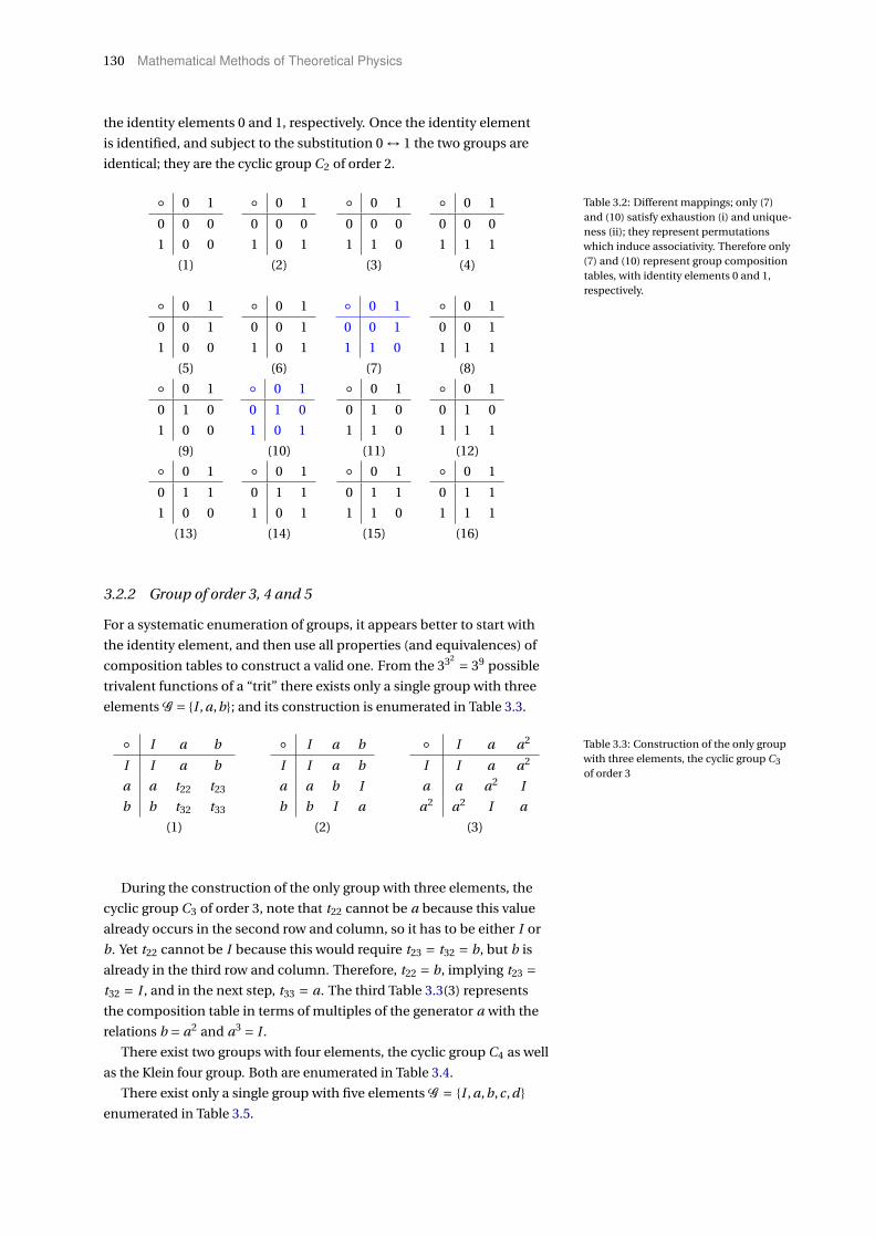
130 Mathematical Methods of Theoretical Physics

the identity elements 0 and 1, respectively. Once the identity element

is identified, and subject to the substitution 0 ↔ 1 the two groups are

identical; they are the cyclic group C2 of order 2.

0 1

0 0 0

1 0 0

0 1

0 0 0

1 0 1

0 1

0 0 0

1 1 0

0 1

0 0 0

1 1 1

(1) (2) (3) (4)

0 1

0 0 1

1 0 0

0 1

0 0 1

1 0 1

0 1

0 0 1

1 1 0

0 1

0 0 1

1 1 1

(5) (6) (7) (8)

0 1

0 1 0

1 0 0

0 1

0 1 0

1 0 1

0 1

0 1 0

1 1 0

0 1

0 1 0

1 1 1

(9) (10) (11) (12)

0 1

0 1 1

1 0 0

0 1

0 1 1

1 0 1

0 1

0 1 1

1 1 0

0 1

0 1 1

1 1 1

(13) (14) (15) (16)

Table 3.2: Different mappings; only (7)and (10) satisfy exhaustion (i) and unique-ness (ii); they represent permutationswhich induce associativity. Therefore only(7) and (10) represent group compositiontables, with identity elements 0 and 1,respectively.

3.2.2 Group of order 3, 4 and 5

For a systematic enumeration of groups, it appears better to start with

the identity element, and then use all properties (and equivalences) of

composition tables to construct a valid one. From the 332 = 39 possible

trivalent functions of a “trit” there exists only a single group with three

elements G = I , a,b; and its construction is enumerated in Table 3.3.

I a b

I I a b

a a t22 t23

b b t32 t33

I a b

I I a b

a a b I

b b I a

I a a2

I I a a2

a a a2 I

a2 a2 I a

(1) (2) (3)

Table 3.3: Construction of the only groupwith three elements, the cyclic group C3of order 3

During the construction of the only group with three elements, the

cyclic group C3 of order 3, note that t22 cannot be a because this value

already occurs in the second row and column, so it has to be either I or

b. Yet t22 cannot be I because this would require t23 = t32 = b, but b is

already in the third row and column. Therefore, t22 = b, implying t23 =t32 = I , and in the next step, t33 = a. The third Table 3.3(3) represents

the composition table in terms of multiples of the generator a with the

relations b = a2 and a3 = I .

There exist two groups with four elements, the cyclic group C4 as well

as the Klein four group. Both are enumerated in Table 3.4.

There exist only a single group with five elements G = I , a,b,c,d

enumerated in Table 3.5.

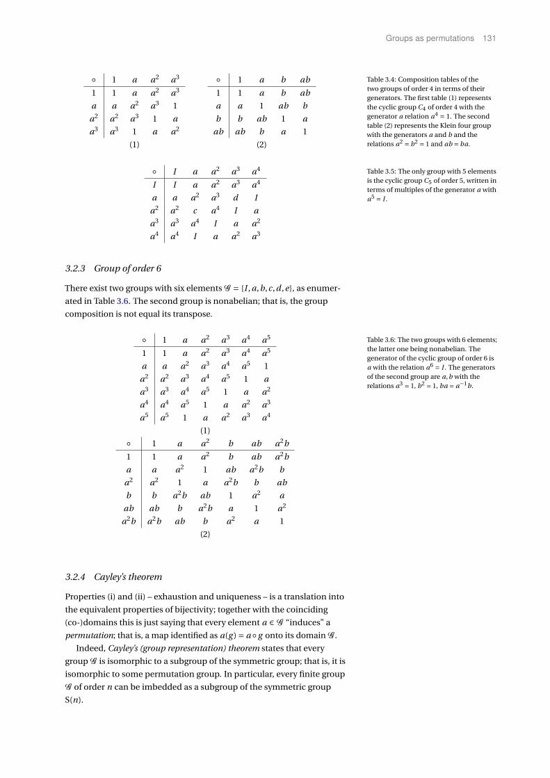
Groups as permutations 131

1 a a2 a3

1 1 a a2 a3

a a a2 a3 1

a2 a2 a3 1 a

a3 a3 1 a a2

1 a b ab

1 1 a b ab

a a 1 ab b

b b ab 1 a

ab ab b a 1

(1) (2)

Table 3.4: Composition tables of thetwo groups of order 4 in terms of theirgenerators. The first table (1) representsthe cyclic group C4 of order 4 with thegenerator a relation a4 = 1. The secondtable (2) represents the Klein four groupwith the generators a and b and therelations a2 = b2 = 1 and ab = ba.

I a a2 a3 a4

I I a a2 a3 a4

a a a2 a3 d I

a2 a2 c a4 I a

a3 a3 a4 I a a2

a4 a4 I a a2 a3

Table 3.5: The only group with 5 elementsis the cyclic group C5 of order 5, written interms of multiples of the generator a witha5 = I .

3.2.3 Group of order 6

There exist two groups with six elements G = I , a,b,c,d ,e, as enumer-

ated in Table 3.6. The second group is nonabelian; that is, the group

composition is not equal its transpose.

1 a a2 a3 a4 a5

1 1 a a2 a3 a4 a5

a a a2 a3 a4 a5 1

a2 a2 a3 a4 a5 1 a

a3 a3 a4 a5 1 a a2

a4 a4 a5 1 a a2 a3

a5 a5 1 a a2 a3 a4

(1)

1 a a2 b ab a2b

1 1 a a2 b ab a2b

a a a2 1 ab a2b b

a2 a2 1 a a2b b ab

b b a2b ab 1 a2 a

ab ab b a2b a 1 a2

a2b a2b ab b a2 a 1

(2)

Table 3.6: The two groups with 6 elements;the latter one being nonabelian. Thegenerator of the cyclic group of order 6 isa with the relation a6 = I . The generatorsof the second group are a,b with therelations a3 = 1, b2 = 1, ba = a−1b.

3.2.4 Cayley’s theorem

Properties (i) and (ii) – exhaustion and uniqueness – is a translation into

the equivalent properties of bijectivity; together with the coinciding

(co-)domains this is just saying that every element a ∈ G “induces” a

permutation; that is, a map identified as a(g ) = a g onto its domain G .

Indeed, Cayley’s (group representation) theorem states that every

group G is isomorphic to a subgroup of the symmetric group; that is, it is

isomorphic to some permutation group. In particular, every finite group

G of order n can be imbedded as a subgroup of the symmetric group

S(n).

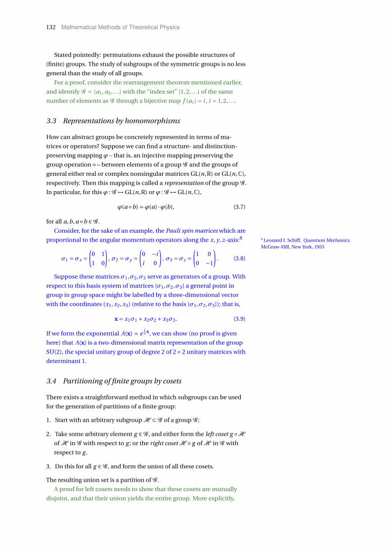
132 Mathematical Methods of Theoretical Physics

Stated pointedly: permutations exhaust the possible structures of

(finite) groups. The study of subgroups of the symmetric groups is no less

general than the study of all groups.

For a proof, consider the rearrangement theorem mentioned earlier,

and identify G = a1, a2, . . . with the “index set” 1,2, . . . of the same

number of elements as G through a bijective map f (ai ) = i , i = 1,2, . . ..

3.3 Representations by homomorphisms

How can abstract groups be concretely represented in terms of ma-

trices or operators? Suppose we can find a structure- and distinction-

preserving mapping ϕ – that is, an injective mapping preserving the

group operation – between elements of a group G and the groups of

general either real or complex nonsingular matrices GL(n,R) or GL(n,C),

respectively. Then this mapping is called a representation of the group G .

In particular, for this ϕ : G 7→ GL(n,R) or ϕ : G 7→ GL(n,C),

ϕ(a b) =ϕ(a) ·ϕ(b), (3.7)

for all a,b, a b ∈G .

Consider, for the sake of an example, the Pauli spin matrices which are

proportional to the angular momentum operators along the x, y , z-axis:8 8 Leonard I. Schiff. Quantum Mechanics.McGraw-Hill, New York, 1955

σ1 =σx =(

0 1

1 0

), σ2 =σy =

(0 −i

i 0

), σ3 =σz =

(1 0

0 −1

). (3.8)

Suppose these matrices σ1,σ2,σ3 serve as generators of a group. With

respect to this basis system of matrices σ1,σ2,σ3 a general point in

group in group space might be labelled by a three-dimensional vector

with the coordinates (x1, x2, x3) (relative to the basis σ1,σ2,σ3); that is,

x = x1σ1 +x2σ2 +x3σ3. (3.9)

If we form the exponential A(x) = ei2 x, we can show (no proof is given

here) that A(x) is a two-dimensional matrix representation of the group

SU(2), the special unitary group of degree 2 of 2×2 unitary matrices with

determinant 1.

3.4 Partitioning of finite groups by cosets

There exists a straightforward method in which subgroups can be used

for the generation of partitions of a finite group:

1. Start with an arbitrary subgroup H ⊂G of a group G ;

2. Take some arbitrary element g ∈G , and either form the left coset g H

of H in G with respect to g ; or the right coset H g of H in G with

respect to g .

3. Do this for all g ∈G , and form the union of all these cosets.

The resulting union set is a partition of G .

A proof for left cosets needs to show that these cosets are mutually

disjoint, and that their union yields the entire group. More explicitly,

Groups as permutations 133

suppose that the two sets formed by g1 H and g2 H are not disjoint. By

this assumption there exist some u1,u2 ∈ H with g1 u1 = g2 u2. Now

take some arbitrary u3 ∈H and form

g2 u3 = g2 u2︸ ︷︷ ︸=g1u1

u−12 u3 = g1 u1 u−1

2 u3︸ ︷︷ ︸∈H︸ ︷︷ ︸

∈H

∈ g1H , (3.10)

and thus we obtain g2 H ⊂ g1 H . A similar, symmetric argument yields

g1 H ⊂ g2 H ; therefore, g2 H = g1 H . That is, stated pointedly, if the

two sets g1 H and g2 H are not disjoint they must be identical. In the

first case of identical sets g1 H = g2 H , H = (g1)−1 g2 H , and thus,

by the rearrangement theorem (cf. Section 3.1.6, page 128), (g1)−1 g2 ∈H .

At the same time, if one considers all g ∈G , and forms g H , already the

elements g I = g recovers the entire group G . (Note that I ∈H .)

For any finite group G and any subgroup H ⊂ G , the relation x ∼ y :x H = y H ⇔ x−1 y ∈H defines an equivalence relation on G . Thereby, This result is part of Lagrange’s theorem in

the mathematics of group theory.the set x H with x ∈ G is a left coset of H in G with respect to g . A

similar statement applies to right cosets.

In the following example we shall consider the symmetric group S(3)

on a set of 3 elements, say, the set of three numbers 1,2,3. In cycle

notation the group can be written as The cycle notation is a compact repre-sentation of permutations, suppressingconstant elements not changed, andwriting the changed elements (num-bers) without commas, starting witha left (unclosed) bracket sign “(” andfrom an arbitrary element i (mostlythe first if an order exists), and writingconsecutive permutations σ(i ), σ(σ(i )),σ(σ(σ(i ))), . . . of this element until theoriginal “seed” i is reached again; atthis point the initial, unclosed bracketis closed by a right bracket sign “)”; e.g.,(1σ(1) . . .σ(σ(i ))σ(σ(σ(. . . (1) . . .))).

S(3) = () ≡ I , (12), (13), (23), (123), (132). (3.11)

The respective subgroups of S(3) are

H1 = (), H2 = (), (12), H3 = (), (13),

H4 = (), (23), H5 = (), (123), (132). (3.12)

Take, for the sake of an example, as a starting point the subgroup

H2 = (), (12) of S(3), and generate the associated partition of S(3) by

forming the left cosets g H for all group elements g ∈G ; that is,

()H2 = () (), () (12) = (), (12) =H2,

(12)H2 = (12) (), (12) (12) = (12), () =H2,

(13)H2 = (13) (), (13) (12) = (13), (123),

(23)H2 = (23) (), (23) (12) = (23), (132),

(123)H2 = (123) (), (123) (12) = (123), (13),

(132)H2 = (132) (), (132) (12) = (132), (23); (3.13)

thereby effectively rendering the following partitioning of S(3) enumer-

ated in (3.11):

PH2 [S(3)] = (), (12)︸ ︷︷ ︸H2

, (13), (123), (23), (132). (3.14)

Similar calculations yield the partitions associated with different

subgroups:

PH1 [S(3)] = (), (12), (13), (23), (123), (132),

PH3 [S(3)] = H3, (12), (132), (23), (123),

PH4 [S(3)] = H4, (12), (123), (13), (132),

PH5 [S(3)] = H5, (12), (13), (23), PS(3) [S(3)] = S(3). (3.15)

134 Mathematical Methods of Theoretical Physics

For quantum computation links tothe hidden subgroup problem seeSection 5.4.3 of Michael A. Nielsen andI. L. Chuang. Quantum Computationand Quantum Information. CambridgeUniversity Press, Cambridge, 2010. D O I :10.1017/CBO9780511976667. URL https:

//doi.org/10.1017/CBO9780511976667.10th Anniversary Edition.

In quantum information theory the hidden subgroup problem is the

problem to find (the generators of) some unknown subgroup H which

is “hidden” by a function f (G ) = X which maps elements of a group G

onto some set X ; while at the same time being constant on the cosets

of G ; more precisely, f (g1) = f (g2) if and only if g1 and g2 belong to the

same coset g1H = g2H of G – the function f represents or “encodes” the

cosets of G by being constant on any single coset while being different

between the different cosets of G .

3.5 Lie theory

Lie groups9 are continuous groups described by several real parameters. 9 Brian C. Hall. An elementaryintroduction to groups and rep-resentations, 2000. URL https:

//arxiv.org/abs/math-ph/0005032;and Brian C. Hall. Lie Groups, Lie Algebras,and Representations. An ElementaryIntroduction, volume 222 of GraduateTexts in Mathematics. Springer Interna-tional Publishing, Cham, Heidelberg, NewYork, Dordrecht, London, second edition,2003,2015. ISBN 978-3-319-13466-6,978-3-319-37433-8. D O I : 10.1007/978-3-319-13467-3. URL https://doi.org/10.

1007/978-3-319-13467-3

3.5.1 Generators

We can generalize this example by defining the generators of a continu-

ous group as the first coefficient of a Taylor expansion around unity; that

is if the dimension of the group is n, and the Taylor expansion is

G(X) =n∑

i=1Xi Ti + . . . , (3.16)

then the matrix generator Ti is defined by

Ti = ∂G(X)

∂Xi

∣∣∣∣X=0

. (3.17)

3.5.2 Exponential map

There is an exponential connection exp : X 7→ G between a matrix Lie

group and the Lie algebra X generated by the generators Ti .

3.5.3 Lie algebra

A Lie algebra is a vector space X , together with a binary Lie bracket

operation [·, ·] : X ×X 7→X satisfying

(i) bilinearity;

(ii) antisymmetry: [X ,Y ] =−[Y , X ], in particular [X , X ] = 0;

(iii) the Jacobi identity: [X , [Y , Z ]]+ [Z , [X ,Y ]]+ [Y , [Z , X ]] = 0

for all X ,Y , Z ∈X .

3.6 Zoology of some important continuous groups

3.6.1 General linear group GL(n,C)

The general linear group GL(n,C) contains all nonsingular (i.e., invert-

ible; there exist an inverse) n ×n matrices with complex entries. The

composition rule “” is identified with matrix multiplication (which is

associative); the neutral element is the unit matrix In = diag(1, . . . ,1︸ ︷︷ ︸n times

).

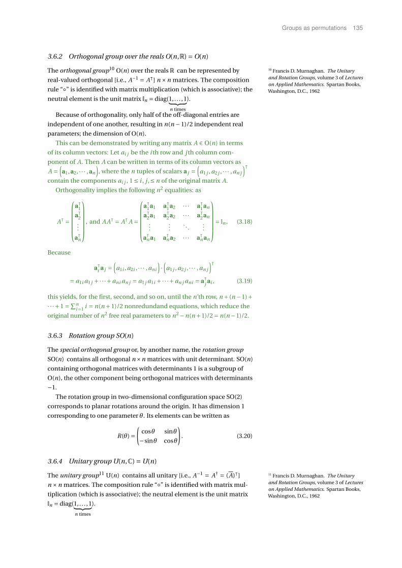
Groups as permutations 135

3.6.2 Orthogonal group over the reals O(n,R) = O(n)

The orthogonal group10 O(n) over the reals R can be represented by 10 Francis D. Murnaghan. The Unitaryand Rotation Groups, volume 3 of Lectureson Applied Mathematics. Spartan Books,Washington, D.C., 1962

real-valued orthogonal [i.e., A−1 = Aᵀ] n ×n matrices. The composition

rule “” is identified with matrix multiplication (which is associative); the

neutral element is the unit matrix In = diag(1, . . . ,1︸ ︷︷ ︸n times

).

Because of orthogonality, only half of the off-diagonal entries are

independent of one another, resulting in n(n −1)/2 independent real

parameters; the dimension of O(n).

This can be demonstrated by writing any matrix A ∈ O(n) in terms

of its column vectors: Let ai j be the i th row and j th column com-

ponent of A. Then A can be written in terms of its column vectors as

A =(a1,a2, · · · ,an

), where the n tuples of scalars a j =

(a1 j , a2 j , · · · , an j

)ᵀcontain the components ai j , 1 ≤ i , j ,≤ n of the original matrix A.

Orthogonality implies the following n2 equalities: as

Aᵀ =

aᵀ

1

aᵀ2...

aᵀn

, and A Aᵀ = AᵀA =

aᵀ

1a1 aᵀ1a2 · · · aᵀ

1an

aᵀ2a1 aᵀ

2a2 · · · aᵀ2an

......

. . ....

aᵀn a1 aᵀ

n a2 · · · aᵀn an

= In , (3.18)

Because

aᵀi a j =

(a1i , a2i , · · · , ani

)·(a1 j , a2 j , · · · , an j

)ᵀ= a1i a1 j +·· ·+ani an j = a1 j a1i +·· ·+an j ani = aᵀ

j ai , (3.19)

this yields, for the first, second, and so on, until the n’th row, n + (n −1)+·· ·+1 =∑n

i=1 i = n(n +1)/2 nonredundand equations, which reduce the

original number of n2 free real parameters to n2 −n(n+1)/2 = n(n−1)/2.

3.6.3 Rotation group SO(n)

The special orthogonal group or, by another name, the rotation group

SO(n) contains all orthogonal n×n matrices with unit determinant. SO(n)

containing orthogonal matrices with determinants 1 is a subgroup of

O(n), the other component being orthogonal matrices with determinants

−1.

The rotation group in two-dimensional configuration space SO(2)

corresponds to planar rotations around the origin. It has dimension 1

corresponding to one parameter θ. Its elements can be written as

R(θ) =(

cosθ sinθ

−sinθ cosθ

). (3.20)

3.6.4 Unitary group U(n,C) = U(n)

The unitary group11 U(n) contains all unitary [i.e., A−1 = A† = (A)ᵀ] 11 Francis D. Murnaghan. The Unitaryand Rotation Groups, volume 3 of Lectureson Applied Mathematics. Spartan Books,Washington, D.C., 1962

n ×n matrices. The composition rule “” is identified with matrix mul-

tiplication (which is associative); the neutral element is the unit matrix

In = diag(1, . . . ,1︸ ︷︷ ︸n times

).

136 Mathematical Methods of Theoretical Physics

For similar reasons as mentioned earlier only half of the off-diagonal

entries – in total (n − 1)+ (n − 2)+ ·· · + 1 = ∑n−1i=1 i = n(n − 1)/2 – are

independent of one another, yielding twice as much – that is, n(n −1) –

conditions for the real parameters. Furthermore the diagonal elements

of A A† = In must be real and one, yielding n conditions. The resulting

number of independent real parameters is 2n2 −n(n −1)−n = n2.

Not that, for instance, U(1) is the set of complex numbers z = e iθ of

unit modulus |z|2 = 1. It forms an Abelian group.

3.6.5 Special unitary group SU(n)

The special unitary group SU(n) contains all unitary n ×n matrices with

unit determinant. SU(n) is a subgroup of U(n).

Since there is one extra condition detA = 1 (with respect to unitary

matrices) the number of independent parameters for SU(n) is n2 −1.

We mention without proof that U(2), which generates all normalized

vectors – identified with pure quantum states– in two-dimensional

Hilbert space from some given arbitrary vector, is 2 : 1 isomorphic to the

rotation group SO(3); that is, more precisely SU (2)/±I = SU (2)/Z2∼=

SO(3). This is the basis of the Bloch sphere representation of pure states

in two-dimensional Hilbert space.

3.6.6 Symmetric group S(n)

The symmetric group S(n) on a finite set of n elements (or symbols) is The symmetric group should not beconfused with a symmetry group.the group whose elements are all the permutations of the n elements,

and whose group operation is the composition of such permutations.

The identity is the identity permutation. The permutations are bijective

functions from the set of elements onto itself. The order (number of

elements) of S(n) is n!.

3.6.7 Poincaré group

The Poincaré group is the group of isometries – that is, bijective maps

preserving distances – in space-time modelled by R4 endowed with a

scalar product and thus of a norm induced by the Minkowski metric

η≡ ηi j = diag(1,1,1,−1) introduced in (2.66).

It has dimension ten (4+3+3 = 10), associated with the ten fundamental

(distance preserving) operations from which general isometries can be

composed: (i) translation through time and any of the three dimensions

of space (1+3 = 4), (ii) rotation (by a fixed angle) around any of the three

spatial axes (3), and a (Lorentz) boost, increasing the velocity in any of

the three spatial directions of two uniformly moving bodies (3).

The rotations and Lorentz boosts form the Lorentz group.

]

Projective and incidence geometry 137

4Projective and incidence geometry

P RO J E C T I V E G E O M E T RY is about the geometric properties that are

invariant under projective transformations. Incidence geometry is about

which points lie on which line.

4.1 Notation

In what follows, for the sake of being able to formally represent geometric

transformations as “quasi-linear” transformations and matrices, the co-

ordinates of n-dimensional Euclidean space will be augmented with one

additional coordinate which is set to one. The following presentation will

use two dimensions, but a generalization to arbitrary finite dimensions

should be straightforward. For instance, in the plane R2, we define new

“three-component” coordinates (with respect to some basis) by

x =(

x1

x2

)≡

x1

x2

1

= X. (4.1)

In order to differentiate these new coordinates X from the usual ones x,

they will be written in capital letters.

4.2 Affine transformations map lines into lines as well as

parallel lines to parallel lines

In what follows we shall consider transformations which map lines into

lines; and, likewise, parallel lines to parallel lines. A theorem of affine

geometry,1 essentially states that these are the affine transformations

1 Wilson Stothers. The Klein view ofgeometry. URL https://www.maths.

gla.ac.uk/wws/cabripages/klein/

klein0.html. accessed on January31st, 2019; K. W. Gruenberg and A. J.Weir. Linear Geometry, volume 49 ofGraduate Texts in Mathematics. Springer-Verlag New York, New York, Heidelberg,Berlin, second edition, 1977. ISBN978-1-4757-4101-8. D O I : 10.1007/978-1-4757-4101-8. URL https://doi.

org/10.1007/978-1-4757-4101-8;and Shiri Artstein-Avidan and Boaz A.Slomka. The fundamental theorems ofaffine and projective geometry revisited.Communications in ContemporaryMathematics, 19(05):1650059, 2016.D O I : 10.1142/S0219199716500590.URL https://doi.org/10.1142/

S0219199716500590

f (x) =Ax+ t (4.2)

with the translation t, encoded by a tuple (t1, t2)ᵀ, and an arbitrary linear

transformation A represented by its associated matrix. Examples of A are

rotations, as well as dilatations and skewing transformations.

Those two operations – the linear transformation A combined with a

“standalone” translation by the vector t – can be “wrapped together” to

138 Mathematical Methods of Theoretical Physics

form the “enlarged” transformation matrix (with respect to some basis;

“0ᵀ” indicates a row matrix with entries zero)

f=(

A t

0ᵀ 1

)≡

a11 a12 t1

a21 a22 t2

0 0 1

. (4.3)

Therefore, the affine transformation f can be represented in the “quasi-

linear” form

f(X) = fX =(

A t

0ᵀ 1

)X. (4.4)

Let us prove sufficiency of the aforementioned theorem of affine

geometry by explicitly showing that an arbitrary affine transformation of

the form (4.3), when applied to the parameter form of the line

L =

y1

y2

1

∣∣∣∣∣∣∣y1

y2

1

=

x1

x2

0

s +

a1

a2

1

=

x1s +a1

x2s +a2

1

, s ∈R

, (4.5)

again yields a line of the form (4.5). Indeed, applying (4.3) to (4.5) yields

fL =

a11 a12 t1

a21 a22 t2

0 0 1

x1s +a1

x2s +a2

1

=

a11(x1s +a1)+a12(x2s +a2)+ t1

a21(x1s +a1)+a22(x2s +a2)+ t2

1

=

(a11x1 +a12x2)s︸ ︷︷ ︸=x′

1s

+a11a1 +a12a2 + t1︸ ︷︷ ︸=a′

1

(a11x1 +a22x2)s︸ ︷︷ ︸=x′

2s

+a21a1 +a22a2 + t2︸ ︷︷ ︸=a′

2

1

= L′.

(4.6)

Another, more elegant, way of demonstrating this property of affine

maps in a standard notation2 is by representing a line with direction 2 Wilson Stothers. The Klein view ofgeometry. URL https://www.maths.gla.

ac.uk/wws/cabripages/klein/klein0.

html. accessed on January 31st, 2019

vector x through the point a by l = sx+ a, with x =(x1, x2

)ᵀand a =(

a1, a2

)ᵀ, and arbitrary s. Applying an affine transformation f=A+ t with

t =(t1, t2

)ᵀ, because of linearity of the matrix A, yields

f(l) =A (sx+a)+ t = sAx+Aa+ t = l′, (4.7)

which is again a line; but one with direction vector Ax through the point

Aa+ t.

The preservation of the “parallel line” property can be proven by

considering a second line m supposedly parallel to the first line l, which

means that m has an identical direction vector x as l. Because the affine

transformation f(m) yields an identical direction vector Ax for m as for l,

both transformed lines remain parallel.

It is not too difficult to prove [by the compound of two transfor-

mations of the affine form (4.3)] that two or more successive affine

transformations again render an affine transformation.

A proper affine transformation is invertible, reversible and one-to-one.

We state without proof that this is equivalent to the invertibility of A and

Projective and incidence geometry 139

thus |A| 6= 0. If A−1 exists then the inverse transformation with respect

to (4.4) is

f−1 =(

A t

0ᵀ 1

)−1

=(A−1 −A−1t

0ᵀ 1

)

= 1

a11a22 −a12a21

a22 −a12 (−a22t1 +a12t2)

−a21 a11 (a21t1 −a11t2)

0 0 (a11a22 −a12a21)

. (4.8)

This can be directly checked by concatenation of f and f−1; that is, by

ff−1 = f−1f = I3: with A−1 = 1a11a22−a12a21

(a22 −a12

−a21 a22

). Consequently

the proper affine transformations form a group (with the unit element

represented by a diagonal matrix with entries 1), the affine group.

As mentioned earlier affine transformations preserve the “parallel

line” property. But what about non-collinear lines? The fundamental

theorem of affine geometry3 states that, given two lists L = a,b,c and 3 Wilson Stothers. The Klein view ofgeometry. URL https://www.maths.gla.

ac.uk/wws/cabripages/klein/klein0.

html. accessed on January 31st, 2019

L′ = a′,b′,c′ of non-collinear points of R2; then there is a unique proper

A set of points are non-collinear if theydont lie on the same line; that is, theirassociated vectors from the origin arelinear independent.

affine transformation mapping L to L′ (and vice versa).

For the sake of convenience we shall first prove the “0,e1,e2 theorem”

stating that if L = p,q,r is a list of non-collinear points of R2, then there

is a unique proper affine transformation mapping 0,e1,e2 to L = p,q,r;

whereby 0 =(0,0

)ᵀ, e1 =

(1,0

)ᵀ, and e2 =

(0,1

)ᵀ: First note that because

p, q, and r are non-collinear by assumption, (q−p) and (r−p) are non-

parallel. Therefore, (q−p) and (r−p) are linear independent.

Next define f to be some affine transformation which maps 0,e1,e2

to L = p,q,r; such that

f(0) =A0+b = b = p, f(e1) =Ae1 +b = q, f(e2) =Ae2 +b = r. (4.9)

Now consider a column vector representation of A =(a1,a2

)with

a1 =(a11, a21

)ᵀand a2 =

(a12, a22

)ᵀ, respectively. Because of the special

form of e1 =(1,0

)ᵀand e2 =

(0,1

)ᵀ,

f(e1) =Ae1 +b = a1 +b = q, f(e2) =Ae2 +b = a2 +b = r. (4.10)

Therefore,

a1 = q−b = q−p, a2 = r−b = r−p. (4.11)

Since by assumption (q−p) and (r−p) are linear independent, so are

a1 and a2. Therefore, A =(a1,a2

)is invertible; and together with the

translation vector b = p, forms a unique affine transformation f which

maps 0,e1,e2 to L = p,q,r.

The fundamental theorem of affine geometry can be obtained by a

conatenation of (inverse) affine transformations of 0,e1,e2: as by the

“0,e1,e2 theorem” there exists a unique (invertible) affine transforma-

tion f connecting 0,e1,e2 to L, as well as a unique affine transformation

g connecting 0,e1,e2 to L′, the concatenation of f−1 with g forms a

compound affine transformation gf−1 mapping L to L′.

140 Mathematical Methods of Theoretical Physics

4.2.1 One-dimensional case

In one dimension, that is, for z ∈C, among the five basic operations

(i) scaling: f(z) = r z for r ∈R,

(ii) translation: f(z) = z+w for w ∈C,

(iii) rotation: f(z) = e iϕz for ϕ ∈R,

(iv) complex conjugation: f(z) = z,

(v) inversion: f(z) = z−1,

there are three types of affine transformations (i)–(iii) which can be

combined.

An example of a one-dimensional case is the “conversion” of prob-

abilities to expectation values in a dichotonic system; say, with ob-

servables in −1,+1. Suppose p+1 = 1− p−1 is the probability of the

occurrence of the observable “+1”. Then the expectation value is

given by E = (+1)p+1 + (−1)p−1 = p+1 − (1− p+1) = 2p+1 − 1; that is,

a scaling of p+1 by a factor of 2, and a translation by −1. Its inverse is

p+1 = (E +1)/2 = E/2+1/2. The respective matrix representation are(2 −1

0 1

)and 1

2

(1 1

0 2

).

For more general dichotomic observables in a,b, E = apa +bpb =apa +b(1−pa) = (a −b)pa +b, so that the matrices representing these

affine transformations are

((a −b) b

0 1

)and 1

a−b

(1 −b

0 a −b

).

4.3 Similarity transformations

Similarity transformations involve translations t, rotations R and a

dilatation r and can be represented by the matrix

(r R t

0ᵀ 1

)≡

m cosϕ −m sinϕ t1

m sinϕ m cosϕ t2

0 0 1

. (4.12)

4.4 Fundamental theorem of affine geometry revisedFor a proof and further references, seeJune A. Lester. Distance preservingtransformations. In Francis Buekenhout,editor, Handbook of Incidence Geometry,pages 921–944. Elsevier, Amsterdam,1995.

Any bijection from Rn , n ≥ 2, onto itself which maps all lines onto lines is

an affine transformation.

4.5 Alexandrov’s theoremFor a proof and further references, seeJune A. Lester. Distance preservingtransformations. In Francis Buekenhout,editor, Handbook of Incidence Geometry,pages 921–944. Elsevier, Amsterdam,1995.

Consider the Minkowski space-timeMn ; that is, Rn , n ≥ 3, and the

Minkowski metric [cf. (2.66) on page 95] η ≡ ηi j = diag(1,1, . . . ,1︸ ︷︷ ︸n−1 times

,−1).

Consider further bijections f fromMn onto itself preserving light cones;

that is for all x,y ∈Mn ,

ηi j (xi − y i )(x j − y j ) = 0 if and only if ηi j (fi (x)− fi (y))(f j (x)− f j (y)) = 0.

Projective and incidence geometry 141

Then f(x) is the product of a Lorentz transformation and a positive scale

factor.

b

Part IIFunctional analysis

Brief review of complex analysis 145

5Brief review of complex analysis

Is it not amazing that complex numbers1 can be used for physics? Robert

1 Edmund Hlawka. Zum Zahlbegriff.Philosophia Naturalis, 19:413–470, 1982

Musil (an Austrian novelist and mathematician), in “Verwirrungen

des Zögling Törleß”2, has expressed the amazement of a youngster

2 German original http://www.gutenberg.org/ebooks/34717: “In solcheiner Rechnung sind am Anfang ganzsolide Zahlen, die Meter oder Gewichte,oder irgend etwas anderes Greifbaresdarstellen können und wenigstens wirk-liche Zahlen sind. Am Ende der Rechnungstehen ebensolche. Aber diese beiden hän-gen miteinander durch etwas zusammen,das es gar nicht gibt. Ist das nicht wieeine Brücke, von der nur Anfangs- undEndpfeiler vorhanden sind und die mandennoch so sicher überschreitet, als obsie ganz dastünde? Für mich hat so eineRechnung etwas Schwindliges; als ob esein Stück des Weges weiß Gott wohin ginge.Das eigentlich Unheimliche ist mir aberdie Kraft, die in solch einer Rechnungsteckt und einen so festhält, daß man dochwieder richtig landet.”

confronted with the applicability of imaginaries, by stating that, at the

beginning of any computation involving imaginary numbers are “solid”

numbers which could represent something measurable, like lengths

or weights, or something else tangible; or are at least real numbers. At

the end of the computation, there are also such “solid” entities. But the

beginning and the end of the computation are connected by something

seemingly nonexisting. Does this not appear, Musil’s Zögling Törleß

wonders, like a bridge crossing an abyss with only a bridge pier at the

very beginning and one at the very end, which could nevertheless be

crossed with certainty and securely, as if this bridge would exist entirely?

In what follows, a very brief review of complex analysis, or, by another

term, theory of complex functions, will be presented. For much more

detailed introductions to complex analysis, including proofs, take, for

instance, a “classical” introduction,3among a zillion of other very good

3 Reinhold Remmert. Theory of ComplexFunctions, volume 122 of GraduateTexts in Mathematics. Springer-Verlag,New York, NY, 1 edition, 1991. ISBN978-1-4612-0939-3,978-0-387-97195-7,978-1-4612-6953-3. D O I : 10.1007/978-1-4612-0939-3. URL https://doi.org/10.

1007/978-1-4612-0939-3

ones.4 We shall study complex analysis not only for its beauty but also

4 Eberhard Freitag and Rolf Busam. Com-plex Analysis. Springer, Berlin, Heidelberg,2005; E. T. Whittaker and G. N. Watson. ACourse of Modern Analysis. CambridgeUniversity Press, Cambridge, fourthedition, 1927. URL http://archive.org/

details/ACourseOfModernAnalysis.Reprinted in 1996. Table errata: Math.Comp. v. 36 (1981), no. 153, p. 319;Robert E. Greene and Stephen G. Krantz.Function theory of one complex variable,volume 40 of Graduate Studies in Mathe-matics. American Mathematical Society,Providence, Rhode Island, third edition,2006; Einar Hille. Analytic Function Theory.Ginn, New York, 1962. 2 Volumes; andLars V. Ahlfors. Complex Analysis: An Intro-duction of the Theory of Analytic Functionsof One Complex Variable. McGraw-HillBook Co., New York, third edition, 1978

because it yields very important analytical methods and tools; for in-

stance for the solution of (differential) equations and the computation

of definite integrals. These methods will then be required for the compu-

tation of distributions and Green’s functions, as well for the solution of

differential equations of mathematical physics – such as the Schrödinger

equation.

One motivation for introducing imaginary numbers is the (if you

perceive it that way) “malady” that not every polynomial such as P (x) =x2 +1 has a root x – and thus not every (polynomial) equation P (x) =x2 +1 = 0 has a solution x – which is a real number. Indeed, you need the

imaginary unit i 2 =−1 for a factorization P (x) = (x + i )(x − i ) yielding the

two roots ±i to achieve this. In that way, the introduction of imaginary

numbers is a further step towards omni-solvability. No wonder that

the fundamental theorem of algebra, stating that every non-constant

polynomial with complex coefficients has at least one complex root – and

thus total factorizability of polynomials into linear factors follows!

If not mentioned otherwise, it is assumed that the Riemann surface,

146 Mathematical Methods of Theoretical Physics

representing a “deformed version” of the complex plane for functional

purposes, is simply connected. Simple connectedness means that the

Riemann surface is path-connected so that every path between two

points can be continuously transformed, staying within the domain, into

any other path while preserving the two endpoints between the paths. In

particular, suppose that there are no “holes” in the Riemann surface; it is

not “punctured.”

Furthermore, let i be the imaginary unit with the property that i 2 =−1

is the solution of the equation x2 +1 = 0. The introduction of imaginary

numbers guarantees that all quadratic equations have two roots (i.e.,

solutions).

By combining imaginary and real numbers, any complex number can

be defined to be some linear combination of the real unit number “1”

with the imaginary unit number i that is, z = 1× (ℜz)+ i × (ℑz), with

the real valued factors (ℜz) and (ℑz), respectively. By this definition, a

complex number z can be decomposed into real numbers x, y , r and ϕ

such that

zdef= ℜz + iℑz = x + i y = r e iϕ = r e i arg(z), (5.1)

with x = r cosϕ and y = r sinϕ, where Euler’s formula

e iϕ = cosϕ+ i sinϕ (5.2)

has been used. If z = ℜz we call z a real number. If z = iℑz we call z a

purely imaginary number. The argument or phase arg(z) of the complex

number z is the angle ϕ (usually in radians) measured counterclockwise

from the positive real axis to the vector representing z in the complex

plane. The principal value Arg(z) is usually defined to lie in the interval

(−π,π]; that is,

−π< Arg(z) ≤+π. (5.3)

Note that the function ϕ 7→ e iϕ in (5.1) is not injective. In particular,

exp(iϕ) = exp(i (ϕ+ 2πk) for arbitrary k ∈ Z. This has no immediate

consequence on z; but it yields differences for functions thereof, like the

square root or the logarithm. A remedy is the introduction of Riemann

surfaces which are “extended” and “deformed” versions of the complex

plane.

The modulus or absolute value of a complex number z is defined by

|z| def= +√

(ℜz)2 + (ℑz)2. (5.4)

Many rules of classical arithmetic can be carried over to complex

arithmetic.5 Note, however, that, because of noninjectivity of exp(iϕ) 5 Tom M. Apostol. Mathematical Analysis:A Modern Approach to Advanced Calculus.Addison-Wesley Series in Mathematics.Addison-Wesley, Reading, MA, secondedition, 1974. ISBN 0-201-00288-4; andEberhard Freitag and Rolf Busam. Funktio-nentheorie 1. Springer, Berlin, Heidelberg,fourth edition, 1993,1995,2000,2006

for arbitrary values of ϕ, for instance,p

ap

b = pab is only valid if at

least one factor a or b is positive; otherwise one could construct wrong

deductions −1 = i 2 ?=p

i 2p

i 2 ?= p−1p−1

?=√

(−1)2 = 1. More gener-

ally, for two arbitrary numbers, u and v ,p

up

v is not always equal topuv . The n’th root of a complex number z parameterized by many (in-

Nevertheless,p|u|p|v | =p|uv |.deed, an infinity of) angles ϕ is no unique function any longer, as npz =

np|z|exp(iϕ/n +2πi k/n

)with k ∈ Z. Thus, in particular, for the square

root with n = 2,p

up

v = p|u| |v |exp[(i /2)(ϕu +ϕv )

]exp[iπ(ku +kv )]︸ ︷︷ ︸

±1

.

Brief review of complex analysis 147

Therefore, with u =−1 = exp[iπ(1+2k)] and v =−1 = exp[iπ(1+2k ′)] and

k,k ′ ∈ Z, one obtainsp−1

p−1 = exp[(i /2)(π+π)]︸ ︷︷ ︸1

exp[iπ(k +k ′)

]︸ ︷︷ ︸±1

= ∓1,

for even and odd k +k ′, respectively.

For many mathematicians Euler’s identity

e iπ =−1, or e iπ+1 = 0, (5.5)

is the “most beautiful” theorem.6 6 David Wells. Which is the most beautiful?The Mathematical Intelligencer, 10:30–31, 1988. ISSN 0343-6993. D O I :10.1007/BF03023741. URL https:

//doi.org/10.1007/BF03023741

Euler’s formula (5.2) can be used to derive de Moivre’s formula for

integer n (for non-integer n the formula is multi-valued for different

arguments ϕ):

e i nϕ = (cosϕ+ i sinϕ)n = cos(nϕ)+ i sin(nϕ). (5.6)

5.1 Geometric representations of complex numbers and

functions thereof

5.1.1 The complex plane

It is quite suggestive to consider the complex numbers z, which are linear

combinations of the real and the imaginary unit, in the complex plane

C=R×R as a geometric representation of complex numbers. Thereby, the

real and the imaginary unit are identified with the (orthonormal) basis

vectors of the standard (Cartesian) basis; that is, with the tuples

1 ≡(1,0

), and i ≡

(0,1

). (5.7)

Figure 5.1 depicts this schema, including the location of the points

corresponding to the real and imaginary units 1 and i , respectively.

ℑz

ℜz

i

1

3+ i

1−2i

−2+2i

− 52 −3i

0

Figure 5.1: Complex plane with dashedunit circle around origin and some points

The addition and multiplication of two complex numbers represented

by(x, y

)and

(u, v

)with x, y ,u, v ∈R are then defined by(

x, y)+

(u, v

)=

(x +u, y + v

),(

x, y)·(u, v

)=

(xu − y v , xv + yu

), (5.8)

and the neutral elements for addition and multiplication are(0,0

)and(

1,0), respectively.

We shall also consider the extended plane C=C∪ ∞ consisting of the

entire complex plane C together with the point “∞” representing infinity.

Thereby, ∞ is introduced as an ideal element, completing the one-to-one

(bijective) mapping w = 1z , which otherwise would have no image at

z = 0, and no pre-image (argument) at w = 0.

5.1.2 Multi-valued relationships, branch points, and branch cuts

Earlier we encountered problems with the square root function on

complex numbers. We shall use this function as a sort of “Rosetta stone”

for an understanding of conceivable ways of coping with nonunique

functional values. Note that even in the real case there are issues: for

positive real numbers we can uniquely define the square root function

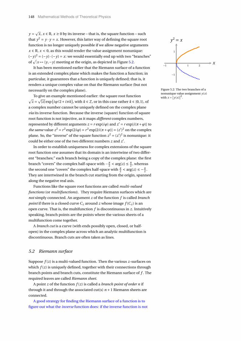
148 Mathematical Methods of Theoretical Physics

y = px, x ∈ R, x ≥ 0 by its inverse – that is, the square function – such

that y2 = y · y = x. However, this latter way of defining the square root

function is no longer uniquely possible if we allow negative arguments

x ∈ R, x < 0, as this would render the value assignment nonunique:

(−y)2 = (−y) · (−y) = x: we would essentially end up with two “branches”

ofp

:x 7→ y ,−y meeting at the origin, as depicted in Figure 5.2.−1 1 2

−1

1

x

y2 = x

Figure 5.2: The two branches of anonunique value assignment y(x)with x = [

y(x)]2.

It has been mentioned earlier that the Riemann surface of a function

is an extended complex plane which makes the function a function; in

particular, it guarantees that a function is uniquely defined; that is, it

renders a unique complex value on that the Riemann surface (but not

necessarily on the complex plane).

To give an example mentioned earlier: the square root functionpz =p|z|exp

(iϕ/2+ iπk

), with k ∈ Z, or in this case rather k ∈ 0,1, of

a complex number cannot be uniquely defined on the complex plane

via its inverse function. Because the inverse (square) function of square

root function is not injective, as it maps different complex numbers,

represented by different arguments z = r exp(iϕ) and z ′ = r exp[i (π+ϕ)] to

the same value z2 = r 2 exp(2iϕ) = r 2 exp[2i (π+ϕ)] = (z ′)2 on the complex

plane. So, the “inverse” of the square function z2 = (z ′)2 is nonunique: it

could be either one of the two different numbers z and z ′.In order to establish uniqueness for complex extensions of the square

root function one assumes that its domain is an intertwine of two differ-

ent “branches;” each branch being a copy of the complex plane: the first

branch “covers” the complex half-space with −π2 < arg(z) ≤ π

2 , whereas

the second one “covers” the complex half-space with π2 < arg(z) ≤ −π

2 .

They are intertwined in the branch cut starting from the origin, spanned

along the negative real axis.

Functions like the square root functions are called multi-valued

functions (or multifunctions). They require Riemann surfaces which are

not simply connected. An argument z of the function f is called branch

point if there is a closed curve Cz around z whose image f (Cz ) is an

open curve. That is, the multifunction f is discontinuous in z. Intuitively

speaking, branch points are the points where the various sheets of a

multifunction come together.

A branch cut is a curve (with ends possibly open, closed, or half-

open) in the complex plane across which an analytic multifunction is

discontinuous. Branch cuts are often taken as lines.

5.2 Riemann surface

Suppose f (z) is a multi-valued function. Then the various z-surfaces on

which f (z) is uniquely defined, together with their connections through

branch points and branch cuts, constitute the Riemann surface of f . The

required leaves are called Riemann sheet.

A point z of the function f (z) is called a branch point of order n if

through it and through the associated cut(s) n +1 Riemann sheets are

connected.

A good strategy for finding the Riemann surface of a function is to

figure out what the inverse function does: if the inverse function is not

Brief review of complex analysis 149

injective on the complex plane, then the function is nonunique. For

example, in the case of the square root function, the inverse function is

the square w : z 7→ z2 = r 2 exp[2i arg(z)] which covers the complex plane

twice during the variation of the principal value −π< arg(z) ≤+π. Thus

the Riemann surface of an inverse function of the square function, that is,

the square function has to have two sheets to be able to cover the original

complex plane of the argument. otherwise, with the exception of the

origin, the square root would be nonunique, and the same point on the

complex w plane would correspond to two distinct points in the original

z-plane. This is depicted in Figure 5.3, where c 6= d yet c2 = d 2.

ℑz

ℜza

b

cd

ℑw

ℜw

b2

a2

c2

ℑw

ℜw

a2

b2

d 2

z = r e i arg(z) w(z) = z2 = r 2e2i arg(z) w(z) = z2 = r 2e2i arg(z)

−π< arg(z) ≤+π −π2 < arg(z) ≤+π

2 +π2 < arg(z) ≤−π

2

Figure 5.3: Sketch of the Riemann surfaceof the square root function, requiring twosheets with the origin as branch point,as argued from the inverse (in this casesquare) function.

5.3 Differentiable, holomorphic (analytic) function

Consider the function f (z) on the domain G ⊂ Domain( f ).

f is called differentiable at the point z0 if the differential quotient

d f

d z

∣∣∣∣z0

= f ′(z)∣∣

z0= ∂ f

∂x

∣∣∣∣z0

= 1

i

∂ f

∂y

∣∣∣∣z0

(5.9)

exists.

If f is (arbitrarily often) differentiable in the domain G it is called

holomorphic. We shall state without proof that, if a holomorphic function

is differentiable, it is also arbitrarily often differentiable.

If a function can be expanded as a convergent power series, like

f (z) =∑∞n=0 an zn , in the domain G then it is called analytic in the domain

G . We state without proof that holomorphic functions are analytic, and

vice versa; that is the terms “holomorphic” and “analytic” will be used

synonymously.

5.4 Cauchy-Riemann equations

The function f (z) = u(z)+ i v(z) (where u and v are real valued functions)

is analytic or holomorphic if and only if (ab = ∂a/∂b)

ux = vy , uy =−vx . (5.10)

150 Mathematical Methods of Theoretical Physics

For a proof, differentiate along the real, and then along the imaginary

axis, taking

f ′(z) = limx→0

f (z +x)− f (z)

x= ∂ f

∂x= ∂u

∂x+ i

∂v

∂x,

and f ′(z) = limy→0

f (z + i y)− f (z)

i y= ∂ f

∂i y=−i

∂ f

∂y=−i

∂u

∂y+ ∂v

∂y. (5.11)

For f to be analytic, both partial derivatives have to be identical, and

thus ∂ f∂x = ∂ f

∂i y , or∂u

∂x+ i

∂v

∂x=−i

∂u

∂y+ ∂v

∂y. (5.12)

By comparing the real and imaginary parts of this equation, one obtains

the two real Cauchy-Riemann equations

∂u

∂x= ∂v

∂y,

∂v

∂x=−∂u

∂y. (5.13)

5.5 Definition analytical function

If f is analytic in G , all derivatives of f exist, and all mixed derivatives are

independent on the order of differentiations. Then the Cauchy-Riemann

equations imply that

∂

∂x

(∂u

∂x

)= ∂

∂x

(∂v

∂y

)= ∂

∂y

(∂v

∂x

)=− ∂

∂y

(∂u

∂y

),

and∂

∂y

(∂v

∂y

)= ∂

∂y

(∂u

∂x

)= ∂

∂x

(∂u

∂y

)=− ∂

∂x

(∂v

∂x

), (5.14)

and thus (∂2

∂x2 + ∂2

∂y2

)u = 0, and

(∂2

∂x2 + ∂2

∂y2

)v = 0. (5.15)

If f = u + i v is analytic in G , then the lines of constant u and v are

orthogonal.

The tangential vectors of the lines of constant u and v in the two-

dimensional complex plane are defined by the two-dimensional nabla

operator ∇u(x, y) and ∇v(x, y). Since, by the Cauchy-Riemann equations

ux = vy and uy =−vx

∇u(x, y) ·∇v(x, y) =(

ux

uy

)·(

vx

vy

)= ux vx +uy vy = ux vx + (−vx )ux = 0

(5.16)

these tangential vectors are normal.

f is angle (shape) preserving conformal if and only if it is holomorphic

and its derivative is everywhere non-zero.

Consider an analytic function f and an arbitrary path C in the com-

plex plane of the arguments parameterized by z(t), t ∈R. The image of C

associated with f is f (C ) =C ′ : f (z(t )), t ∈R.

The tangent vector of C ′ in t = 0 and z0 = z(0) is

d

d tf (z(t ))

∣∣∣∣t=0

= d

d zf (z)

∣∣∣∣z0

d

d tz(t )

∣∣∣∣t=0

=λ0e iϕ0d

d tz(t )

∣∣∣∣t=0

. (5.17)

Brief review of complex analysis 151

Note that the first term dd z f (z)

∣∣∣z0

is independent of the curve C and only

depends on z0. Therefore, it can be written as a product of a squeeze

(stretch) λ0 and a rotation e iϕ0 . This is independent of the curve; hence

two curves C1 and C2 passing through z0 yield the same transformation

of the image λ0e iϕ0 .

5.6 Cauchy’s integral theorem

If f is analytic on G and on its borders ∂G , then any closed line integral of

f vanishes ∮∂G

f (z)d z = 0. (5.18)

No proof is given here.

In particular,∮

C⊂∂G f (z)d z is independent of the particular curve and

only depends on the initial and the endpoints.

For a proof, subtract two line integral which follow arbitrary paths

C1 and C2 to a common initial and end point, and which have the same

integral kernel. Then reverse the integration direction of one of the line

integrals. According to Cauchy’s integral theorem, the resulting integral

over the closed loop has to vanish.

Often it is useful to parameterize a contour integral by some form of∫C

f (z)d z =∫ b

af (z(t ))

d z(t )

d td t . (5.19)

Let f (z) = 1/z and C : z(ϕ) = Re iϕ, with R > 0 and −π<ϕ≤π. Then∮|z|=R

f (z)d z =∫ π

−πf (z(ϕ))

d z(ϕ)

dϕdϕ

=∫ π

−π1

Re iϕR i e iϕdϕ

=∫ π

−πiϕ

= 2πi (5.20)

is independent of R.

5.7 Cauchy’s integral formula

If f is analytic on G and on its borders ∂G , then

f (z0) = 1

2πi

∮∂G

f (z)

z − z0d z. (5.21)

No proof is given here.

Note that because of Cauchy’s integral formula, analytic functions

have an integral representation. This has far-reaching consequences:

because analytic functions have integral representations, their higher

derivatives also have integral representations. And, as a result, if a func-

tion has one complex derivative, then it has infinitely many complex

derivatives. This statement can be formally expressed by the generalized

Cauchy integral formula or, by another term, by Cauchy’s differentiation

formula states that if f is analytic on G and on its borders ∂G , then

f (n)(z0) = n!2πi

∮∂G

f (z)

(z − z0)n+1 d z. (5.22)

152 Mathematical Methods of Theoretical Physics

No proof is given here.

Cauchy’s integral formula presents a powerful method to compute

integrals. Consider the following examples.

1. First, let us calculate ∮|z|=3

3z +2

z(z +1)3 d z.

The kernel has two poles at z = 0 and z =−1 which are both inside the

domain of the contour defined by |z| = 3. By using Cauchy’s integral

formula we obtain for “small” ε ∮|z|=3

3z +2

z(z +1)3 d z

=∮|z|=ε

3z +2

z(z +1)3 d z +∮|z+1|=ε

3z +2

z(z +1)3 d z

=∮|z|=ε

3z +2

(z +1)3

1

zd z +

∮|z+1|=ε

3z +2

z

1

(z +1)3 d z

= 2πi

0!d 0

d z0︸︷︷︸1

3z +2

(z +1)3

∣∣∣∣∣∣∣∣z=0

+ 2πi

2!d 2

d z2

3z +2

z

∣∣∣∣z=−1

= 2πi

0!3z +2

(z +1)3

∣∣∣∣z=0

+ 2πi

2!d 2

d z2

3z +2

z︸ ︷︷ ︸4(−1)2z−3

∣∣∣∣∣∣∣∣∣z=−1

= 4πi −4πi = 0. (5.23)

2. Consider ∮|z|=3

e2z

(z +1)4 d z

= 2πi

3!3!

2πi

∮|z|=3

e2z

(z − (−1))3+1 d z

= 2πi

3!d 3

d z3

∣∣e2z ∣∣z=−1

= 2πi

3!23 ∣∣e2z ∣∣

z=−1

= 8πi e−2

3. (5.24)

Suppose g (z) is a function with a pole of order n at the point z0; that is

g (z) = f (z)

(z − z0)n , (5.25)

where f (z) is an analytic function. Then,∮∂G

g (z)d z = 2πi

(n −1)!f (n−1)(z0). (5.26)

5.8 Series representation of complex differentiable functions

As a consequence of Cauchy’s (generalized) integral formula, analytic

functions have power series representations.

Brief review of complex analysis 153

For the sake of a proof, we shall recast the denominator z − z0 in

Cauchy’s integral formula (5.21) as a geometric series as follows (we shall

assume that |z0 −a| < |z −a|)1

z − z0= 1

(z −a)− (z0 −a)

= 1

(z −a)

[1

1− z0−az−a

]

= 1

(z −a)

[ ∞∑n=0

(z0 −a)n

(z −a)n

]=

∞∑n=0

(z0 −a)n

(z −a)n+1 . (5.27)

By substituting this in Cauchy’s integral formula (5.21) and using

Cauchy’s generalized integral formula (5.22) yields an expansion of

the analytical function f around z0 by a power series

f (z0) = 1

2πi

∮∂G

f (z)

z − z0d z

= 1

2πi

∮∂G

f (z)∞∑

n=0

(z0 −a)n

(z −a)n+1 d z

=∞∑

n=0(z0 −a)n 1

2πi

∮∂G

f (z)

(z −a)n+1 d z

=∞∑

n=0

f n(z0)

n!(z0 −a)n . (5.28)

5.9 Laurent and Taylor series

Every function f which is analytic in a concentric region R1 < |z − z0| < R2

can in this region be uniquely written as a Laurent series

f (z) =∞∑

k=−∞(z − z0)k ak , with coefficients

ak = 1

2πi

∮C

(χ− z0)−k−1 f (χ)dχ. (5.29)

The closed contour C must be in the concentric region.

The coefficient a−1 is called the residue and denoted by “Res:”

Res( f (z0))def= a−1 = 1

2πi

∮C

f (χ)dχ. (5.30)

For a proof, as in Eqs. (5.27) we shall recast (a −b)−1 for |a| > |b| as a

geometric series

1

a −b= 1

a

(1

1− ba

)= 1

a

( ∞∑n=0

bn

an

)=

∞∑n=0

bn

an+1

[substitution n +1 →−k, n →−k −1k →−n −1] =−∞∑

k=−1

ak

bk+1, (5.31)

and, for |a| < |b|,1

a −b=− 1

b −a=−

∞∑n=0

an

bn+1

[substitution n +1 →−k, n →−k −1k →−n −1] =−−∞∑

k=−1

bk

ak+1. (5.32)

154 Mathematical Methods of Theoretical Physics

Furthermore since a +b = a − (−b), we obtain, for |a| > |b|,1

a +b=

∞∑n=0

(−1)n bn

an+1 =−∞∑

k=−1(−1)−k−1 ak

bk+1=−

−∞∑k=−1

(−1)k ak

bk+1, (5.33)

and, for |a| < |b|,1

a +b=−

∞∑n=0

(−1)n+1 an

bn+1 =∞∑

n=0(−1)n an

bn+1

=−∞∑

k=−1(−1)−k−1 bk

ak+1=−

−∞∑k=−1

(−1)k bk

ak+1. (5.34)

Suppose that some function f (z) is analytic in an annulus bounded by

the radius r1 and r2 > r1. By substituting this in Cauchy’s integral formula

(5.21) for an annulus bounded by the radius r1 and r2 > r1 (note that the

orientations of the boundaries with respect to the annulus are opposite,

rendering a relative factor “−1”) and using Cauchy’s generalized integral

formula (5.22) yields an expansion of the analytical function f around

z0 by the Laurent series for a point a on the annulus; that is, for a path

containing the point z around a circle with radius r1, |z − a| < |z0 − a|;likewise, for a path containing the point z around a circle with radius

r2 > a > r1, |z −a| > |z0 −a|,

f (z0) = 1

2πi

∮r1

f (z)

z − z0d z − 1

2πi

∮r2

f (z)

z − z0d z

= 1

2πi

[∮r1

f (z)∞∑

n=0

(z0 −a)n

(z −a)n+1 d z +∮

r2

f (z)−∞∑

n=−1

(z0 −a)n

(z −a)n+1 d z

]= 1

2πi

[ ∞∑n=0

(z0 −a)n∮

r1

f (z)

(z −a)n+1 d z +−∞∑

n=−1(z0 −a)n

∮r2

f (z)

(z −a)n+1 d z

]=

∞∑n=−∞

(z0 −a)n[

1

2πi

∮r1≤r≤r2

f (z)

(z −a)n+1 d z

].

(5.35)

Suppose that g (z) is a function with a pole of order n at the point z0;

that is g (z) = h(z)/(z − z0)n , where h(z) is an analytic function. Then the

terms k ≤−(n +1) vanish in the Laurent series. This follows from Cauchy’s

integral formula

ak = 1

2πi

∮C

(χ− z0)−k−n−1h(χ)dχ= 0 (5.36)

for −k −n −1 ≥ 0.

Note that, if f has a simple pole (pole of order 1) at z0, then it can

be rewritten into f (z) = g (z)/(z − z0) for some analytic function g (z) =(z − z0) f (z) that remains after the singularity has been “split” from f .

Cauchy’s integral formula (5.21), and the residue can be rewritten as

a−1 = 1

2πi

∮∂G

g (z)

z − z0d z = g (z0). (5.37)

For poles of higher order, the generalized Cauchy integral formula (5.22)

can be used.

Suppose that f (z) is analytic at and in a region G “around” z0. Then

the Laurent series (5.29) “turns into” a Taylor series expansion of f (z):

f (z) =∞∑

k=0

f (k)(z0)

k!(z − z0)k , with z ∈G . (5.38)

Brief review of complex analysis 155

For a proof relative to the validity of the Laurent series (5.29), sup-

pose that f (z) is analytic at and “in a region around” z0, and note the

following:

(i) Because of Cauchy’s integral theorem (5.18),

ak<0 =1

2πi

∮C

(χ− z0)|k|−1 f (χ)dχ= 0, (5.39)

since, for k < 0, −k −1 = |k|−1 ≥ 0, and, therefore, (χ− z0)|k|−1 f (χ) is

analytic, too.

(ii) Because of Cauchy’s integral formula (5.21),

ak=0 =1

2πi

∮C

f (χ)

χ− z0dχ= f (z0). (5.40)

(iii) Because of the generalized Cauchy integral formula (aka Cauchy’s

differentiation formula) (5.22),

ak>0 =1

2πi

∮C

f (χ)

(χ− z0)k+1dχ= f (k)(z0)

k!. (5.41)

5.10 Residue theorem

Suppose f is analytic on a simply connected open subset G with the

exception of finitely many (or denumerably many) points zi . Then,∮∂G

f (z)d z = 2πi∑zi

Res f (zi ). (5.42)

No proof is given here.

The residue theorem presents a powerful tool for calculating integrals,

both real and complex. Let us first mention a rather general case of a

situation often used. Suppose we are interested in the integral

I =∫ ∞

−∞R(x)d x

with rational kernel R; that is, R(x) = P (x)/Q(x), where P (x) and Q(x)

are polynomials (or can at least be bounded by a polynomial) with no

common root (and therefore factor). Suppose further that the degrees of

the polynomial are

deg P (x) ≤ deg Q(x)−2.

This condition is needed to assure that the additional upper or lower

path we want to add when completing the contour does not contribute;

that is, vanishes.

Now first let us analytically continue R(x) to the complex plane R(z);

that is,

I =∫ ∞

−∞R(x)d x =

∫ ∞

−∞R(z)d z.

Next let us close the contour by adding a (vanishing) curve integral∫å

R(z)d z = 0

156 Mathematical Methods of Theoretical Physics

in the upper (lower) complex plane

I =∫ ∞

−∞R(z)d z +

∫å

R(z)d z =∮→&å

R(z)d z.

The added integral vanishes because it can be approximated by

∣∣∣∣∫å R(z)d z

∣∣∣∣≤ limr→∞

(const.

r 2 πr

)= 0.

With the contour closed the residue theorem can be applied for an

evaluation of I ; that is,

I = 2πi∑zi

ResR(zi )

for all singularities zi in the region enclosed by “→ & å. ”

Let us consider some examples.

(i) Consider

I =∫ ∞

−∞d x

x2 +1.

The analytic continuation of the kernel and the addition with vanish-

ing a semicircle “far away” closing the integration path in the upper

complex half-plane of z yields

I =∫ ∞

−∞d x

x2 +1

=∫ ∞

−∞d z

z2 +1

=∫ ∞

−∞d z

z2 +1+

∫å

d z

z2 +1

=∫ ∞

−∞d z

(z + i )(z − i )+

∫å

d z

(z + i )(z − i )

=∮

1

(z − i )f (z)d z with f (z) = 1

(z + i )

= 2πi Res

(1

(z + i )(z − i )

)∣∣∣∣z=+i

= 2πi f (+i )

= 2πi1

(2i )=π.

(5.43)

Here, Equation (5.37) has been used. Closing the integration path in

the lower complex half-plane of z yields (note that in this case the

Brief review of complex analysis 157

contour integral is negative because of the path orientation)

I =∫ ∞

−∞d x

x2 +1

=∫ ∞

−∞d z

z2 +1

=∫ ∞

−∞d z

z2 +1+

∫lower path

d z

z2 +1

=∫ ∞

−∞d z

(z + i )(z − i )+

∫lower path

d z

(z + i )(z − i )

=∮

1

(z + i )f (z)d z with f (z) = 1

(z − i )

=−2πi Res

(1

(z + i )(z − i )

)∣∣∣∣z=−i

=−2πi f (−i )

= 2πi1

(2i )=π.

(5.44)

(ii) Consider

F (p) =∫ ∞

−∞e i px

x2 +a2 d x

with a 6= 0.

The analytic continuation of the kernel yields

F (p) =∫ ∞

−∞e i pz

z2 +a2 d z =∫ ∞

−∞e i pz

(z − i a)(z + i a)d z.

Suppose first that p > 0. Then, if z = x + i y , e i pz = e i px e−py → 0 for

z →∞ in the upper half plane. Hence, we can close the contour in the

upper half plane and obtain F (p) with the help of the residue theorem.

If a > 0 only the pole at z = +i a is enclosed in the contour; thus we

obtain

F (p) = 2πi Rese i pz

(z + i a)

∣∣∣∣z=+i a

= 2πie i 2pa

2i a

= π

ae−pa . (5.45)

If a < 0 only the pole at z = −i a is enclosed in the contour; thus we

obtain

F (p) = 2πi Rese i pz

(z − i a)

∣∣∣∣z=−i a

= 2πie−i 2pa

−2i a

= π

−ae−i 2pa

= π

−aepa . (5.46)

Hence, for a 6= 0,

F (p) = π

|a|e−|pa|. (5.47)

158 Mathematical Methods of Theoretical Physics

For p < 0 a very similar consideration, taking the lower path for contin-

uation – and thus acquiring a minus sign because of the “clockwork”

orientation of the path as compared to its interior – yields

F (p) = π

|a|e−|pa|. (5.48)

(iii) If some function f (z) can be expanded into a Taylor series or Lau-

rent series, the residue can be directly obtained by the coefficient

of the 1z term. For instance, let f (z) = e

1z and C : z(ϕ) = Re iϕ, with

R = 1 and −π<ϕ≤π. This function is singular only in the origin z = 0,

but this is an essential singularity near which the function exhibits

extreme behavior. Nevertheless, f (z) = e1z can be expanded into a

Laurent series

f (z) = e1z =

∞∑l=0

1

l !

(1

z

)l

around this singularity. The residue can be found by using the series

expansion of f (z); that is, by comparing its coefficient of the 1/z term.

Hence, Res(e

1z

)∣∣∣z=0

is the coefficient 1 of the 1/z term. Thus,∮|z|=1

e1z d z = 2πi Res

(e

1z

)∣∣∣z=0

= 2πi . (5.49)

For f (z) = e−1z , a similar argument yields Res

(e−

1z

)∣∣∣z=0

=−1 and thus∮|z|=1 e−

1z d z =−2πi .

An alternative attempt to compute the residue, with z = e iϕ, yields

a−1 = Res(e±

1z

)∣∣∣z=0

= 1

2πi

∮C

e±1z d z

= 1

2πi

∫ π

−πe± 1

eiϕd z(ϕ)

dϕdϕ

=± 1

2πi

∫ π

−πe± 1

eiϕ i e±iϕdϕ

=± 1

2π

∫ π

−πe±e∓iϕ

e±iϕdϕ

=± 1

2π

∫ π

−πe±e∓iϕ±iϕdϕ. (5.50)

5.11 Some special functional classes

5.11.1 Criterion for coincidence

The requirement that a function is holomorphic (analytic, differentiable)

puts some stringent conditions on its type, form, and on its behavior.

For instance, let z0 ∈ G the limit of a sequence zn ∈ G , zn 6= z0. Then it

can be shown that, if two analytic functions f and g on the domain G

coincide in the points zn , then they coincide on the entire domain G .

5.11.2 Entire function

An function is said to be an entire function if it is defined and differ-

entiable (holomorphic, analytic) in the entire finite complex plane C.

Brief review of complex analysis 159

An entire function may be either a rational function f (z) = P (z)/Q(z)

which can be written as the ratio of two polynomial functions P (z) and

Q(z), or it may be a transcendental function such as ez or sin z.

The Weierstrass factorization theorem states that an entire function

can be represented by a (possibly infinite7) product involving its zeroes 7 Theodore W. Gamelin. Complex Analysis.Springer, New York, 2001[i.e., the points zk at which the function vanishes f (zk ) = 0]. For example

(for a proof, see Equation (6.2) of,8) 8 J. B. Conway. Functions of ComplexVariables. Volume I. Springer, New York,1973

sin z = z∞∏

k=1

[1−

( z

πk

)2]

. (5.51)

5.11.3 Liouville’s theorem for bounded entire function

Liouville’s theorem states that a bounded [that is, the (principal, positive)

square root of its absolute square is finite everywhere in C] entire func-

tion which is defined at infinity is a constant. Conversely, a nonconstant

entire function cannot be bounded. It may (wrongly) appear that sin z isnonconstant and bounded. However, itis only bounded on the real axis; indeed,sin i y = (1/2i )(e−y − e y ) = i sinh y .Likewise, cos i y = cosh y .

For a proof, consider the integral representation of the derivative f ′(z)

of some bounded entire function | f (z)| <C <∞ with bound C , obtained

through Cauchy’s integral formula (5.22), taken along a circular path with

arbitrarily but “large” radius r À 1 of length 2πr in the limit of infinite

radius; that is, ∣∣ f ′(z0)∣∣= ∣∣∣∣ 1

2πi

∮∂G

f (z)

(z − z0)2 d z

∣∣∣∣=

∣∣∣∣ 1

2πi

∣∣∣∣ ∣∣∣∣∮∂G

f (z)

(z − z0)2 d z

∣∣∣∣< 1

2π

∮∂G

∣∣ f (z)∣∣

(z − z0)2 d z

< 1

2π2πr

C

r 2 = C

rr→∞−→ 0. (5.52)

As a result, f (z0) = 0 and thus f = A ∈C.

Note that, as (uv) = (u) (v), so is |uv |2 =uv(uv) = u(u) v(v) = |u|2 |v |2.

A generalized Liouville theorem states that if f : C→ C is an entire

function, and if, for some real number C and some positive integer k,

f (z) is bounded by | f (z)| ≤ C |z|k for all z with |z| ≥ 0, then f (z) is a

polynomial in z of degree at most k.

For a proof of the generalized Liouville theorem we exploit the fact

that f is analytic on the entire complex plane. Thus it can be expanded

into a Taylor series (5.38) about z0:

f (z) =∞∑

l=0al (z − z0)l , with al =

f (l )(z0)

l !. (5.53)

Now consider the integral representation of the l th derivative f (l )(z) of

some bounded entire function | f (z)| <C |z|k with bound C <∞, obtained

through Cauchy’s integral formula (5.22), and taken along a circular

path with arbitrarily but “large” radius r À 1 of length 2πr in the limit of

infinite radius; that is, ∣∣∣ f (l )(z0)∣∣∣= ∣∣∣∣ 1

2πi

∮∂G

f (z)

(z − z0)l+1d z

∣∣∣∣=

∣∣∣∣ 1

2πi

∣∣∣∣ ∣∣∣∣∮∂G

f (z)

(z − z0)l+1d z

∣∣∣∣< 1

2π

∮∂G

∣∣ f (z)∣∣

(z − z0)l+1d z

< 1

2π2πrCr k−l−1 =Cr k−l

r→∞l>k−→ 0. (5.54)

160 Mathematical Methods of Theoretical Physics

As a result, f (z) =∑kl=0 al (z − z0)l , with al ∈C.

Liouville’s theorem is important for an investigation into the general

form of the Fuchsian differential equation on page 235.

5.11.4 Picard’s theorem

Picard’s theorem states that any entire function that misses two or more

points f : C 7→ C− z1, z2, . . . is constant. Conversely, any nonconstant

entire function covers the entire complex plane C except a single point.

An example of a nonconstant entire function is ez which never reaches

the point 0.

5.11.5 Meromorphic function

If f has no singularities other than poles in the domain G it is called

meromorphic in the domain G .

We state without proof (e.g., Theorem 8.5.1 of Ref. 9) that a function

9 Einar Hille. Analytic Function Theory.Ginn, New York, 1962. 2 Volumes

f which is meromorphic in the extended plane is a rational function

f (z) = P (z)/Q(z) which can be written as the ratio of two polynomial

functions P (z) and Q(z).

5.12 Fundamental theorem of algebra

For a discussion and proofs, see, forinstance, Chapter 19 of Martin Aignerand Günter M. Ziegler. Proofs fromTHE BOOK. Springer, Heidelberg, fouredition, 1998-2010. ISBN 978-3-642-00856-6,978-3-642-00855-9. D O I : 10.1007/978-3-642-00856-6. URL https://doi.

org/10.1007/978-3-642-00856-6, orChapter 4 (by Remmert) of Heinz-DieterEbbinghaus, Hans Hermes, FriedrichHirzebruch, Max Koecher, Klaus Mainzer,Jürgen Neukirch, Alexander Prestel, andReinhold Remmert. Numbers, volume123 of Readings in Mathematics. Springer-Verlag New York, New York, NY, 1991. ISBN978-1-4612-1005-4. D O I : 10.1007/978-1-4612-1005-4. URL https://doi.org/10.

1007/978-1-4612-1005-4. Translated byH. L. S. Orde.

The factor theorem states that a polynomial P (z) in z of degree k has a

factor z − z0 if and only if P (z0) = 0, and can thus be written as P (z) =(z − z0)Q(z), where Q(z) is a polynomial in z of degree k −1. Hence, by

iteration,

P (z) =αk∏

i=1(z − zi ) , (5.55)

where α ∈C.

No proof is presented here.

The fundamental theorem of algebra states that every polynomial

(with arbitrary complex coefficients) has a root [i.e. solution of f (z) = 0]

in the complex plane. Therefore, by the factor theorem, the number of

roots of a polynomial, up to multiplicity, equals its degree.

Again, no proof is presented here.

5.13 Asymptotic series

Asymtotic series occur in physics in the context of “perturbative” or

series solutions of ordinary differential equations. they will be studied

in the last Chapter 12. In what follows we shall closely follow Remmert’s

exposition.10

10 Reinhold Remmert. Theory of ComplexFunctions, volume 122 of GraduateTexts in Mathematics. Springer-Verlag,New York, NY, 1 edition, 1991. ISBN978-1-4612-0939-3,978-0-387-97195-7,978-1-4612-6953-3. D O I : 10.1007/978-1-4612-0939-3. URL https://doi.org/10.

1007/978-1-4612-0939-3

In what follows a formal (power) series sn(z) = ∑nj=0 a j z j is called an

asymptotic development or, equivalently, an asymptotic representation or

asymptotic expansion of some holomorphic function f in a domain G at

the border point 0 ∈ ∂G ∈G if the asymptotic series “approximates” f at 0;

that is, if

limz→0

1

zn

[f (z)−

n∑j=0

a j z j

]= 0 for every n ∈N. (5.56)

Brief review of complex analysis 161

Alternatively and equivalently, asymptoticity can be defined as follows:11

11 Frank Olver. Asymptotics and specialfunctions. AKP classics. A.K. Peters/CRCPress/Taylor & Francis, New York, NY, 2ndedition, 1997. ISBN 9780429064616. D O I :10.1201/9781439864548. URL https:

//doi.org/10.1201/9781439864548;Carl M. Bender and Steven A. Orszag.Andvanced Mathematical Methods forScientists and Enineers I. AsymptoticMethods and Perturbation Theory.International Series in Pure and AppliedMathematics. McGraw-Hill and Springer-Verlag, New York, NY, 1978,1999. ISBN978-1-4757-3069-2,978-0-387-98931-0,978-1-4419-3187-0. D O I : 10.1007/978-1-4757-3069-2. URL https://doi.org/10.

1007/978-1-4757-3069-2; and John P.Boyd. The devil’s invention: Asymptotic,superasymptotic and hyperasymptoticseries. Acta Applicandae Mathematica,56:1–98, 1999. ISSN 0167-8019. D O I :10.1023/A:1006145903624. URL https:

//doi.org/10.1023/A:1006145903624

a (power) series∑n

j=0 a j z j is asymptotic to a function f (z) if, for every

n ∈N and sufficiently small r ,∣∣∣∣∣ f (z)−n∑

j=0a j z j

∣∣∣∣∣=O(r N+1) ; (5.57)

where O represents the big O notation, or, used synonymously, the

Bachmann-Landau notation or asymptotic notation12. 12 The symbol “O” stands for “of theorder of” or “absolutely bound by” inthe following way: if g (x) is a positivefunction, then f (x) =O

(g (x)

)implies that

there exist a positive real number m suchthat | f (x)| < mg (x).

In this case we introduce the following “∼G ”notation:

f (z) ∼G

∞∑j=0

a j z j . (5.58)

Note that the asymptotic expansion of any holomorphic function f in a

domain G at the border point 0 ∈ ∂G ∈G is unique; the coefficients a j can

be found iteratively by

a0 = limz→0

f (z), and

an = limz→0

1

zn

[f (z)−

n−1∑j=0

a j z j

]for n > 0.

To obtain a feeling for this type of asymptotic expansion, consider the

following holomorphic functions:

1. the constant function f (z) = c. In this case, a0 = c, and all other an = 0

for n > 0;

2. the function f (z) = cez . In this case, by using the Taylor expansion for

ez , one recovers that same Taylor series:

a0 = limz→0

cez = ce0 = c,

a1 = limz→0

1

z

[cez − c

]= limz→0

[cz0 +O(z1)

]= c,

a2 = limz→0

1

z2

[cez − c − cz

]= limz→0

[c

1

2!z0 +O(z1)

]= c

2!,

...

ak = limz→0

1

zk

[cez − c

n−1∑j=1

z j

j !

]= lim

z→0

[c

1

n!z0 +O(z1)

]= c

n!.

Is the converse also true? That is, given an arbitrary asymptotic

sequence on a domain; does there exist an associated holomorphic

function such that the former sequence yields an asymptotic expansion

of the latter function?

A similar question can be asked for Taylor expansions: let (a j )∞j=0 be

an infinite sequence of numbers whose Taylor series∑∞

j=01j ! a j z j at z = 0

converges (with positive radius of convergence r ). This Taylor series then

defines a unique analytic function f (z) =∑∞j=0

1j ! a j z j which is uniquely

defined in a circular domain with radius r and center z = 0.

However, if we allow also functions g (z) which are not necessarily

analytic, then the Taylor series g (z) =∑∞j=0

1j ! a j z j is not unique, because

g (z) = f (z)+d(z) would also be represented by one and the same Taylor

162 Mathematical Methods of Theoretical Physics

series if only d(0) = 0 as well as all of the derivatives vanish at z = 0; that

is, if d (n)(0) = 0 for n = 0,1,2, . . . . Take, for example, d(z) = exp(− 1

z2

)for

x 6= 0 and d(0) = 0, which is a variant of the class-I test function with

compact support [cf. Equation (7.12) on page 175]: d is smooth but not

analytic.

Let us now come back to the general case of not necessarily converg-

ing power series with arbitrary coefficients ai . The following theorem

of Ritt gives a positive answer but does not guarantee uniqueness of

the function: Associated with every infinite power series∑∞

j=0 a j z j with

arbitrary complex coefficients a j corresponds a holomorphic function

f in a proper circular sector G at z=0 such that (5.58) holds; that is,13

13 For proper definitions, proofs andfurther details see Franz Pittnauer. Vor-lesungen über asymptotische Reihen,volume 301 of Lecture Notes in Mathemat-ics. Springer Verlag, Berlin Heidelberg,1972. ISBN 978-3-540-38077-1,978-3-540-06090-1. D O I : 10.1007/BFb0059524. URLhttps://doi.org/10.1007/BFb0059524,Reinhold Remmert. Theory of ComplexFunctions, volume 122 of Graduate Textsin Mathematics. Springer-Verlag, NewYork, NY, 1 edition, 1991. ISBN 978-1-4612-0939-3,978-0-387-97195-7,978-1-4612-6953-3. D O I : 10.1007/978-1-4612-0939-3.URL https://doi.org/10.1007/

978-1-4612-0939-3 and Ovidiu Costin.Asymptotics and Borel Summability,volume 141 of Monographs and surveys inpure and applied mathematics. Chapman& Hall/CRC, Taylor & Francis Group, BocaRaton, FL, 2009. ISBN 9781420070316.URL https://www.crcpress.com/

Asymptotics-and-Borel-Summability/

Costin/p/book/9781420070316.

∑∞j=0 a j z j ∼G f (z).

The idea of Ritt’s theorem is elegant and not too difficult to compre-

hend: define a series

f (z)def=

∞∑j=0

a j z j f j (z) ≡∞∑

j=0a j z j f ( j , z) (5.59)

with additional “convergence factors” f j (z) ≡ f ( j , z) which should

perform according to two criteria:

1. f j (z) ≡ f ( j , z) should become “very small” as a function of j ; that is, as

j grows; so much so that it “compensates” for the term z j ; and

2. at the same time, for every fixed j , limz→0 f j (z) ≡ limz→0 f ( j , z) = 1;

that is, the convergence factors should all converge “sufficiently

rapidly” so as to obtain (5.58); that is,∑∞

j=0 a j z j ∼G f (z).

There may be many functional forms of “convergence factors” satis-

fying the above criteria; therefore the construction cannot yield unique-

ness. One candidate for the “convergence factors” is

f j (z) ≡ f ( j , z) = 1−e− b jp

z , (5.60)

withp

z = elog z

2 and real positive coefficients b j > 0 properly chosen such

that, for all j ∈N,

∣∣∣∣∣1−e− b jp

z

∣∣∣∣∣≤ b j∣∣pz∣∣ , as well as lim

z→0

e− b jp

z

z j. (5.61)

Other (uniform with respect to the summation index j ) convergence

or cutoff factors discussed by Tao14 in § 3.7 are compactly supported 14 Terence Tao. Compactness and con-tradiction. American MathematicalSociety, Providence, RI, 2013. ISBN 978-1-4704-1611-9,978-0-8218-9492-7. URLhttps://terrytao.files.wordpress.

com/2011/06/blog-book.pdf

bounded functions that equals 1 at z = 0; see (7.14) on page 176 for an

example.

c

Brief review of Fourier transforms 163

6Brief review of Fourier transforms

6.0.1 Functional spaces

That complex continuous waveforms or functions are comprised of a

number of harmonics seems to be an idea at least as old as the Pythagore-

ans. In physical terms, Fourier analysis1 attempts to decompose a 1 T. W. Körner. Fourier Analysis. CambridgeUniversity Press, Cambridge, UK, 1988;Kenneth B. Howell. Principles of Fourieranalysis. Chapman & Hall/CRC, BocaRaton, London, New York, Washington,D.C., 2001; and Russell Herman. Introduc-tion to Fourier and Complex Analysis withApplications to the Spectral Analysis ofSignals. University of North Carolina Wilm-ington, Wilmington, NC, 2010. URL http:

//people.uncw.edu/hermanr/mat367/

FCABook/Book2010/FTCA-book.pdf.Creative Commons Attribution-NoncommercialShare Alike 3.0 UnitedStates License

function into its constituent harmonics, known as a frequency spectrum.

Thereby the goal is the expansion of periodic and aperiodic functions

into sine and cosine functions. Fourier’s observation or conjecture is,

informally speaking, that any “suitable” function f (x) can be expressed

as a possibly infinite sum (i.e., linear combination), of sines and cosines

of the form

f (x) =∞∑

k=−∞[Ak cos(C kx)+Bk sin(C kx)]

= −1∑

k=−∞+

∞∑k=0

[Ak cos(C kx)+Bk sin(C kx)]

=∞∑

k=1[A−k cos(−C kx)+B−k sin(−C kx)]

+∞∑

k=0[Ak cos(C kx)+Bk sin(C kx)]

= A0 +∞∑

k=1[(Ak + A−k )cos(C kx)+ (Bk −B−k )sin(C kx)]

= a0

2+

∞∑k=1

[ak cos(C kx)+bk sin(C kx)] , (6.1)

with a0 = 2A0, ak = Ak + A−k , and bk = Bk −B−k .

Moreover, it is conjectured that any “suitable” function f (x) can

be expressed as a possibly infinite sum (i.e. linear combination), of

exponentials; that is,

f (x) =∞∑

k=−∞Dk e i kx . (6.2)

More generally, it is conjectured that any “suitable” function f (x) can

be expressed as a possibly infinite sum (i.e. linear combination), of other

(possibly orthonormal) functions gk (x); that is,

f (x) =∞∑

k=−∞γk gk (x). (6.3)

164 Mathematical Methods of Theoretical Physics

The bigger picture can then be viewed in terms of functional (vector)

spaces: these are spanned by the elementary functions gk , which serve

as elements of a functional basis of a possibly infinite-dimensional

vector space. Suppose, in further analogy to the set of all such functions

G = ⋃k gk (x) to the (Cartesian) standard basis, we can consider these

elementary functions gk to be orthonormal in the sense of a generalized

functional scalar product [cf. also Section 11.5 on page 255; in particular

Equation (11.118)]

⟨gk | gl ⟩ =∫ b

agk (x)gl (x)ρ(x)d x = δkl . (6.4)

For most of our purposes, ρ(x) = 1. One could arrange the coefficients

γk into a tuple (an ordered list of elements) (γ1,γ2, . . .) and consider

them as components or coordinates of a vector with respect to the linear

orthonormal functional basis G .

6.0.2 Fourier series

Suppose that a function f (x) is periodic – that is, it repeats its values in

the interval [− L2 , L

2 ] – with period L. (Alternatively, the function may be

only defined in this interval.) A function f (x) is periodic if there exist a

period L ∈R such that, for all x in the domain of f ,

f (L+x) = f (x). (6.5)

With certain “mild” conditions – that is, f must be piecewise con-

tinuous, periodic with period L, and (Riemann) integrable – f can be

decomposed into a Fourier series

f (x) = a0

2+

∞∑k=1

[ak cos

(2π

Lkx

)+bk sin

(2π

Lkx

)], with

ak = 2

L

L2∫

− L2

f (x)cos

(2π

Lkx

)d x for k ≥ 0

bk = 2

L

L2∫

− L2

f (x)sin

(2π

Lkx

)d x for k > 0. (6.6)

For proofs and additional informationsee § 8.1 in Kenneth B. Howell. Prin-ciples of Fourier analysis. Chapman &Hall/CRC, Boca Raton, London, New York,Washington, D.C., 2001.

For a (heuristic) proof, consider the Fourier conjecture (6.1), and

compute the coefficients Ak , Bk , and C .

First, observe that we have assumed that f is periodic with period

L. This should be reflected in the sine and cosine terms of (6.1), which

themselves are periodic functions, repeating their values in the interval

[−π,π]; with period 2π. Thus in order to map the functional period of f

into the sines and cosines, we can “stretch/shrink” L into 2π; that is, C in

Equation (6.1) is identified with

C = 2π

L. (6.7)

Thus we obtain

f (x) =∞∑

k=−∞

[Ak cos

(2π

Lkx

)+Bk sin

(2π

Lkx

)]. (6.8)

Brief review of Fourier transforms 165

Now use the following properties: (i) for k = 0, cos(0) = 1 and sin(0) = 0.

Thus, by comparing the coefficient a0 in (6.6) with A0 in (6.1) we obtain

A0 = a02 .

(ii) Since cos(x) = cos(−x) is an even function of x, we can rear-

range the summation by combining identical functions cos(− 2πL kx) =

cos( 2πL kx), thus obtaining ak = A−k + Ak for k > 0.

(iii) Since sin(x) = −sin(−x) is an odd function of x, we can rear-

range the summation by combining identical functions sin(− 2πL kx) =

−sin( 2πL kx), thus obtaining bk =−B−k +Bk for k > 0.

Having obtained the same form of the Fourier series of f (x) as ex-

posed in (6.6), we now turn to the derivation of the coefficients ak and

bk . a0 can be derived by just considering the functional scalar product in

Equation (6.4) of f (x) with the constant identity function g (x) = 1; that is,

⟨g | f ⟩ =∫ L

2

− L2

f (x)d x

=∫ L

2

− L2

a0

2+

∞∑n=1

[an cos

(2π

Lnx

)+bn sin

(2π

Lnx

)]d x = a0

L

2, (6.9)

and hence

a0 = 2

L

∫ L2

− L2

f (x)d x (6.10)

In a similar manner, the other coefficients can be computed by con-

sidering⟨

cos( 2π

L kx) | f (x)

⟩ ⟨sin

( 2πL kx

) | f (x)⟩

and exploiting the orthogo-

nality relations for sines and cosines

∫ L2

− L2

sin

(2π

Lkx

)cos

(2π

Ll x

)d x = 0,

∫ L2

− L2

cos

(2π

Lkx

)cos

(2π

Ll x

)d x

=∫ L

2

− L2

sin

(2π

Lkx

)sin

(2π

Ll x

)d x = L

2δkl . (6.11)

For the sake of an example, let us compute the Fourier series of

f (x) = |x| =−x, for −π≤ x < 0,

+x, for 0 ≤ x ≤π.

First observe that L = 2π, and that f (x) = f (−x); that is, f is an even

function of x; hence bn = 0, and the coefficients an can be obtained by

considering only the integration between 0 and π.

For n = 0,

a0 = 1

π

π∫−π

d x f (x) = 2

π

π∫0

xd x =π.

166 Mathematical Methods of Theoretical Physics

For n > 0,

an = 1

π

π∫−π

f (x)cos(nx)d x = 2

π

π∫0

x cos(nx)d x =

= 2

π

sin(nx)

nx

∣∣∣∣π0−

π∫0

sin(nx)

nd x

= 2

π

cos(nx)

n2

∣∣∣∣π0=

= 2

π

cos(nπ)−1

n2 =− 4

πn2 sin2 nπ

2=

0 for even n

− 4

πn2 for odd n

Thus,

f (x) = π

2− 4

π

(cos x + cos3x

9+ cos5x

25+·· ·

)=

= π

2− 4

π

∞∑n=0

cos[(2n +1)x]

(2n +1)2 .

One could arrange the coefficients (a0, a1,b1, a2,b2, . . .) into a tuple

(an ordered list of elements) and consider them as components or

coordinates of a vector spanned by the linear independent sine and

cosine functions which serve as a basis of an infinite dimensional vector

space.

6.0.3 Exponential Fourier series

Suppose again that a function is periodic with period L. Then, under

certain “mild” conditions – that is, f must be piecewise continuous,

periodic with period L, and (Riemann) integrable – f can be decomposed

into an exponential Fourier series

f (x) =∞∑

k=−∞ck e i kx , with

ck = 1

L

∫ L2

− L2

f (x ′)e−i kx ′d x ′. (6.12)

The exponential form of the Fourier series can be derived from the

Fourier series (6.6) by Euler’s formula (5.2), in particular, e i kϕ = cos(kϕ)+i sin(kϕ), and thus

cos(kϕ) = 1

2

(e i kϕ+e−i kϕ

), as well as sin(kϕ) = 1

2i

(e i kϕ−e−i kϕ

).

By comparing the coefficients of (6.6) with the coefficients of (6.12), we

obtain

ak = ck + c−k for k ≥ 0,

bk = i (ck − c−k ) for k > 0, (6.13)

or

ck =

1

2(ak − i bk ) for k > 0,

a0

2for k = 0,

1

2(a−k + i b−k ) for k < 0.

(6.14)

Brief review of Fourier transforms 167

Eqs. (6.12) can be combined into

f (x) = 1

L

∞∑k=−∞

∫ L2

− L2

f (x ′)e−i k(x′−x)d x ′. (6.15)

6.0.4 Fourier transformation

Suppose we define ∆k = 2π/L, or 1/L =∆k/2π. Then Equation (6.15) can

be rewritten as

f (x) = 1

2π

∞∑k=−∞

∫ L2

− L2

f (x ′)e−i k(x ′−x)d x ′∆k. (6.16)

Now, in the “aperiodic” limit L →∞ we obtain the Fourier transformation

and the Fourier inversion F−1[F [ f (x)]] =F [F−1[ f (x)]] = f (x) by

f (x) = 1

2π

∫ ∞

−∞

∫ ∞

−∞f (x ′)e−i k(x′−x)d x ′dk, whereby

F−1[ f ](x) = f (x) =α∫ ∞

−∞f (k)e±i kx dk, and

F [ f ](k) = f (k) =β∫ ∞

−∞f (x ′)e∓i kx ′

d x ′. (6.17)

F [ f (x)] = f (k) is called the Fourier transform of f (x). Per convention,

either one of the two sign pairs +− or −+ must be chosen. The factors α

and β must be chosen such that

αβ= 1

2π; (6.18)

that is, the factorization can be “spread evenly among α and β,” such that

α= β= 1/p

2π, or “unevenly,” such as, for instance, α= 1 and β= 1/2π,

or α= 1/2π and β= 1.

Most generally, the Fourier transformations can be rewritten (change

of integration constant), with arbitrary A,B ∈R, as

F−1[ f ](x) = f (x) = B∫ ∞

−∞f (k)e i Akx dk, and

F [ f ](k) = f (k) = A

2πB

∫ ∞

−∞f (x ′)e−i Akx′

d x ′. (6.19)

The choice A = 2π and B = 1 renders a symmetric form of (6.19); more

precisely,

F−1[ f ](x) = f (x) =∫ ∞

−∞f (k)e2πi kx dk, and

F [ f ](k) = f (k) =∫ ∞

−∞f (x ′)e−2πi kx ′

d x ′. (6.20)

For the sake of an example, assume A = 2π and B = 1 in Equation

(6.19), therefore starting with (6.20), and consider the Fourier transform

of the Gaussian function

ϕ(x) = e−πx2. (6.21)

As a hint, notice that the analytic continuation of e−t 2is analytic in the

region 0 ≤ |Im t | ≤pπ|k|. Furthermore, as will be shown in Eqs. (7.20), the

Gaussian integral is ∫ ∞

−∞e−t 2

d t =pπ. (6.22)

168 Mathematical Methods of Theoretical Physics

With A = 2π and B = 1 in Equation (6.19), the Fourier transform of the

Gaussian function is

F [ϕ](k) = ϕ(k) =∞∫

−∞e−πx2

e−2πi kx d x

[completing the exponent] =∞∫

−∞e−πk2

e−π(x+i k)2d x (6.23)

The variable transformation t = pπ(x + i k) yields d t/d x = p

π; thus

d x = d t/pπ, and

F [ϕ](k) = ϕ(k) = e−πk2

pπ

+∞+ipπk∫

−∞+ipπk

e−t 2d t (6.24)

ℑt

ℜt

k ≥ 0

k ≤ 0

· · · · · ·

· · · · · ·

Figure 6.1: Integration paths to computethe Fourier transform of the Gaussian.

Let us rewrite the integration (6.24) into the Gaussian integral by

considering the closed paths (depending on whether k is positive or neg-

ative) depicted in Fig. 6.1. whose “left and right pieces vanish” strongly as

the real part goes to (minus) infinity. Moreover, by the Cauchy’s integral

theorem, Equation (5.18) on page 151,

∮C

d te−t 2 =−∞∫

+∞e−t 2

d t ++∞+i

pπk∫

−∞+ipπk

e−t 2d t = 0, (6.25)

because e−t 2is analytic in the region 0 ≤ |Im t | ≤ p

π|k|. Thus, by substi-

tuting+∞+i

pπk∫

−∞+ipπk

e−t 2d t =

+∞∫−∞

e−t 2d t , (6.26)

in (6.24) and by insertion of the valuepπ for the Gaussian integral, as

shown in Equation (7.20), we finally obtain

F [ϕ](k) = ϕ(k) = e−πk2

pπ

+∞∫−∞

e−t 2d t

︸ ︷︷ ︸pπ

= e−πk2. (6.27)

A similar calculation yields

F−1[ϕ](x) =ϕ(x) = e−πx2. (6.28)

Eqs. (6.27) and (6.28) establish the fact that the Gaussian function

ϕ(x) = e−πx2defined in (6.21) is an eigenfunction of the Fourier transfor-

mations F and F−1 with associated eigenvalue 1. See Section 6.3 in Robert Strichartz. AGuide to Distribution Theory and FourierTransforms. CRC Press, Boca Roton,Florida, USA, 1994. ISBN 0849382734.

With a slightly different definition the Gaussian function f (x) = e−x2/2

is also an eigenfunction of the operator

H =− d 2

d x2 +x2 (6.29)

corresponding to a harmonic oscillator. The resulting eigenvalue equa-

tion is

H f (x) =(− d 2

d x2 +x2)

e−x22 =− d

d x

(−xe−

x22

)+x2e−

x22

= e−x22 −x2e−

x22 +x2e−

x22 = e−

x22 = f (x); (6.30)

Brief review of Fourier transforms 169

with eigenvalue 1.

Instead of going too much into the details here, it may suffice to say

that the Hermite functions

hn(x) =π−1/4(2nn!)−1/2(

d

d x−x

)n

e−x2/2 =π−1/4(2nn!)−1/2Hn(x)e−x2/2

(6.31)

are all eigenfunctions of the Fourier transform with the eigenvalue

i np

2π. The polynomial Hn(x) of degree n is called Hermite polynomial.

Hermite functions form a complete system, so that any function g (with∫ |g (x)|2d x <∞) has a Hermite expansion

g (x) =∞∑

k=0⟨g ,hn⟩hn(x). (6.32)

This is an example of an eigenfunction expansion.

o

Distributions as generalized functions 171

7Distributions as generalized functions

7.1 Coping with discontinuities and singularities

What follows are “recipes” and a “cooking course” for some “dishes”

Heaviside, Dirac and others have enjoyed “eating,” alas without being

able to “explain their digestion” (cf. the citation by Heaviside on page xii).

Insofar theoretical physics is natural philosophy, the question arises

if “measurable” physical entities need to be “smooth” and “continuous”,1 1 William F. Trench. Introduction to realanalysis. Free Hyperlinked Edition 2.01,2012. URL http://ramanujan.math.

trinity.edu/wtrench/texts/TRENCH_

REAL_ANALYSIS.PDF

as “Nature abhors sudden discontinuities,” or if we are willing to allow

and conceptualize singularities of different sorts. Other, entirely different,

scenarios are discrete, computer-generated universes. This little course

is no place for preference and judgments regarding these matters. Let me

just point out that contemporary mathematical physics is not only lean-

ing toward, but appears to be deeply committed to discontinuities; both

in classical and quantized field theories dealing with “point charges,”

as well as in general relativity, the (nonquantized field theoretical) ge-

ometrodynamics of gravitation, dealing with singularities such as “black

holes” or “initial singularities” of various sorts.

Discontinuities were introduced quite naturally as electromagnetic

pulses, which can, for instance, be described with the Heaviside function

H(t) representing vanishing, zero field strength until time t = 0, when

suddenly a constant electrical field is “switched on eternally.” It is quite

natural to ask what the derivative of the unit step function H(t ) might be.

— At this point, the reader is kindly asked to stop reading for a moment

and contemplate on what kind of function that might be.

Heuristically, if we call this derivative the (Dirac) delta function δ

defined by δ(t ) = d H(t )d t , we can assure ourselves of two of its properties (i)

“δ(t) = 0 for t 6= 0,” as well as the antiderivative of the Heaviside function,

yielding (ii) “∫ ∞−∞δ(t )d t = ∫ ∞

−∞d H(t )

d t d t = H(∞)−H(−∞) = 1−0 = 1.” This heuristic definition of the Diracdelta function δy (x) = δ(x, y) = δ(x − y)with a discontinuity at y is not unlike thediscrete Kronecker symbol δi j . We mayeven define the Kronecker symbol δi j asthe difference quotient of some “discreteHeaviside function” Hi j = 1 for i ≥ j , andHi , j = 0 else: δi j = Hi j −H(i−1) j = 1 onlyfor i = j ; else it vanishes.

Indeed, we could follow a pattern of “growing discontinuity,” reach-

able by ever higher and higher derivatives of the absolute value (or

modulus); that is, we shall pursue the path sketched by

|x|d

d x−→ sgn(x), H(x)d

d x−→ δ(x)dn

d xn−→ δ(n)(x).

Objects like |x|, H(x) = 12

[1+ sgn(x)

]or δ(x) may be heuristically

understandable as “functions” not unlike the regular analytic functions;

172 Mathematical Methods of Theoretical Physics

alas their nth derivatives cannot be straightforwardly defined. In order to

cope with a formally precise definition and derivation of (infinite) pulse

functions and to achieve this goal, a theory of generalized functions, or,

used synonymously, distributions has been developed. In what follows

we shall develop the theory of distributions; always keeping in mind the

assumptions regarding (dis)continuities that make necessary this part of

the calculus.

The Ansatz pursued2 will be to “pair” (that is, to multiply) these 2 J. Ian Richards and Heekyung K.Youn. The Theory of Distributions:A Nontechnical Introduction. Cam-bridge University Press, Cambridge,1990. ISBN 9780511623837. D O I :10.1017/CBO9780511623837. URL https:

//doi.org/10.1017/CBO9780511623837

generalized functions F with suitable “good” test functions ϕ, and

integrate over these functional pairs Fϕ. Thereby we obtain a linear

continuous functional F [ϕ], also denoted by ⟨F ,ϕ⟩. This strategy allows

for the “transference” or “shift” of operations on, and transformations

of, F – such as differentiations or Fourier transformations, but also

multiplications with polynomials or other smooth functions – to the test

function ϕ according to adjoint identities See Sect. 2.3 in Robert Strichartz. AGuide to Distribution Theory and FourierTransforms. CRC Press, Boca Roton,Florida, USA, 1994. ISBN 0849382734.

⟨TF ,ϕ⟩ = ⟨F ,Sϕ⟩. (7.1)

For example, for the n’th derivative,

S= (−1)nT= (−1)n d (n)

d x(n); (7.2)

and for the Fourier transformation,

S= T=F . (7.3)

For some (smooth) functional multiplier g (x) ∈C∞ ,

S= T= g (x). (7.4)

One more issue is the problem of the meaning and existence of weak

solutions (also called generalized solutions) of differential equations for

which, if interpreted in terms of regular functions, the derivatives may

not all exist.

Take, for example, the wave equation in one spatial dimension∂2

∂t 2 u(x, t) = c2 ∂2

∂x2 u(x, t). It has a solution of the form3 u(x, t) = 3 Asim O. Barut. e = ×ω. Physics LettersA, 143(8):349–352, 1990. ISSN 0375-9601.D O I : 10.1016/0375-9601(90)90369-Y. URL https://doi.org/10.1016/

0375-9601(90)90369-Y

f (x − ct )+ g (x + ct ), where f and g characterize a travelling “shape”

of inert, unchanged form. There is no obvious physical reason why the

pulse shape function f or g should be differentiable, alas if it is not, then

u is not differentiable either. What if we, for instance, set g = 0, and

identify f (x − ct ) with the Heaviside infinite pulse function H(x − ct )?

7.2 General distributionA nice video on “Setting Up the FourierTransform of a Distribution” by ProfessorDr. Brad G. Osgood @ Stanford Universityis available via URL https://youtu.be/

47yUeygfj3g

Suppose we have some “function” F (x); that is, F (x) could be either a

regular analytical function, such as F (x) = x, or some other, “weirder, sin-

gular, function,” such as the Dirac delta function, or the derivative of the

Heaviside (unit step) function, which might be “highly discontinuous.”

As an Ansatz, we may associate with this “function” F (x) a distribution,

or, used synonymously, a generalized function F [ϕ] or ⟨F ,ϕ⟩ which in the

“weak sense” is defined as a continuous linear functional by integrating

F (x) together with some “good” test function ϕ as follows:4

4 Laurent Schwartz. Introduction to theTheory of Distributions. University ofToronto Press, Toronto, 1952. collected andwritten by Israel Halperin

Distributions as generalized functions 173

F (x) ←→⟨F ,ϕ⟩ ≡ F [ϕ] =∫ ∞

−∞F (x)ϕ(x)d x. (7.5)

We say that F [ϕ] or ⟨F ,ϕ⟩ is the distribution associated with or induced

by F (x). We can distinguish between a regular and a singular distribu-

tion: a regular distribution can be defined by a continuous function F ;

otherwise it is called singular.

One interpretation of F [ϕ] ≡ ⟨F ,ϕ⟩ is that ϕ stands for a sort of “mea-

surement device” probing F , the “system to be measured.” In this in-

terpretation, F [ϕ] ≡ ⟨F ,ϕ⟩ is the “outcome” or “measurement result.”

Thereby, it completely suffices to say what F “does to” some test function

ϕ; there is nothing more to it.

For example, the Dirac Delta function δ(x), as defined later in Equa-

tion (7.50), is completely characterised by

δ(x) ←→ δ[ϕ] ≡ ⟨δ,ϕ⟩ =ϕ(0);

likewise, the shifted Dirac Delta function δy (x) ≡ δ(x − y) is completely

characterised by

δy (x) ≡ δ(x − y) ←→ δy [ϕ] ≡ ⟨δy ,ϕ⟩ =ϕ(y).

Many other generalized “functions” which are usually not integrable

in the interval (−∞,+∞) will, through the pairing with a “suitable” or

“good” test function ϕ, induce a distribution.

For example, take

1 ←→ 1[ϕ] ≡ ⟨1,ϕ⟩ =∫ ∞

−∞ϕ(x)d x,

or

x ←→ x[ϕ] ≡ ⟨x,ϕ⟩ =∫ ∞

−∞xϕ(x)d x,

or

e2πi ax ←→ e2πi ax [ϕ] ≡ ⟨e2πi ax ,ϕ⟩ =∫ ∞

−∞e2πi axϕ(x)d x.

7.2.1 Duality

Sometimes, F [ϕ] ≡ ⟨F ,ϕ⟩ is also written in a scalar product notation; that

is, F [ϕ] = ⟨F |ϕ⟩. This emphasizes the pairing aspect of F [ϕ] ≡ ⟨F ,ϕ⟩. In

this view, the set of all distributions F is the dual space of the set of test

functions ϕ.

7.2.2 Linearity

Recall that a linear functional is some mathematical entity which maps a

function or another mathematical object into scalars in a linear manner;

that is, as the integral is linear, we obtain

F [c1ϕ1 + c2ϕ2] = c1F [ϕ1]+ c2F [ϕ2]; (7.6)

or, in the bracket notation,

⟨F ,c1ϕ1 + c2ϕ2⟩ = c1⟨F ,ϕ1⟩+ c2⟨F ,ϕ2⟩. (7.7)

This linearity is guaranteed by integration.

174 Mathematical Methods of Theoretical Physics

7.2.3 Continuity

One way of expressing continuity is the following:

if ϕnn→∞−→ ϕ, then F [ϕn]

n→∞−→ F [ϕ], (7.8)

or, in the bracket notation,

if ϕnn→∞−→ ϕ, then ⟨F ,ϕn⟩ n→∞−→ ⟨F ,ϕ⟩. (7.9)

7.3 Test functions

Test functions are useful for a consistent definition of generalized func-

tions. Nevertheless, the results obtained should be independent of their

particular form.

7.3.1 Desiderata on test functions

By invoking test functions, we would like to be able to differentiate

distributions very much like ordinary functions. We would also like

to transfer differentiations to the functional context. How can this be

implemented in terms of possible “good” properties we require from the

behavior of test functions, in accord with our wishes?

Consider the partial integration obtained from (uv)′ = u′v +uv ′; thus∫(uv)′ = ∫

u′v+∫uv ′, and finally

∫u′v = ∫

(uv)′−∫uv ′, thereby effectively

allowing us to “shift” or “transfer” the differentiation of the original

function to the test function. By identifying u with the generalized

function g (such as, for instance δ), and v with the test function ϕ,

respectively, we obtain

⟨g ′,ϕ⟩ ≡ g ′[ϕ] =∫ ∞

−∞g ′(x)ϕ(x)d x

= g (x)ϕ(x)∣∣∞−∞−

∫ ∞

−∞g (x)ϕ′(x)d x

= g (∞)ϕ(∞)︸ ︷︷ ︸should vanish

−g (−∞)ϕ(−∞)︸ ︷︷ ︸should vanish

−∫ ∞

−∞g (x)ϕ′(x)d x

=−g [ϕ′] ≡−⟨g ,ϕ′⟩. (7.10)

We can justify the two main requirements of “good” test functions, at

least for a wide variety of purposes:

1. that they “sufficiently” vanish at infinity – this can, for instance, be

achieved by requiring that their support (the set of arguments x where

g (x) 6= 0) is finite; and

2. that they are continuously differentiable – indeed, by induction, that

they are arbitrarily often differentiable.

In what follows we shall enumerate three types of suitable test func-

tions satisfying these desiderata. One should, however, bear in mind that

the class of “good” test functions depends on the distribution. Take, for

example, the Dirac delta function δ(x). It is so “concentrated” that any

(infinitely often) differentiable – even constant – function f (x) defined

Distributions as generalized functions 175

“around x = 0” can serve as a “good” test function (with respect to δ),

as f (x) is only evaluated at x = 0; that is, δ[ f ] = f (0). This is again an

indication of the duality between distributions on the one hand, and

their test functions on the other hand.

Note that if ϕ(x) is a “good” test function, then

xαPn(x)ϕ(x),α ∈Rn ∈N (7.11)

with any Polynomial Pn(x), and, in particular, xnϕ(x), is also a “good”

test function.

7.3.2 Test function class I

Recall that we require5 our test functions ϕ to be infinitely often differen- 5 Laurent Schwartz. Introduction to theTheory of Distributions. University ofToronto Press, Toronto, 1952. collected andwritten by Israel Halperin

tiable. Furthermore, in order to get rid of terms at infinity “in a straight-

forward, simple way,” suppose that their support is compact. Compact

support means that ϕ(x) does not vanish only at a finite, bounded region

of x. Such a “good” test function is, for instance,

ϕσ,a(x) =

exp

−

[1− ( x−a

σ

)2]−1

for

∣∣ x−aσ

∣∣< 1,

0 else.(7.12)

In order to show that ϕσ,a is a suitable test function, we have to prove

its infinite differentiability, as well as the compactness of its support

Mϕσ,a . Let

ϕσ,a(x) :=ϕ( x −a

σ

)and thus

ϕ(x) =exp

(1

x2−1

)for |x| < 1

0 for |x| ≥ 1.(7.13)

This function is drawn in Figure 7.1.

−2 −1 0 1 2

0

0.1

0.2

0.3

0.4

Figure 7.1: Plot of a test function ϕ(x).

First, note, by definition, the support Mϕ = (−1,1), because ϕ(x)

vanishes outside (−1,1)).

Second, consider the differentiability of ϕ(x); that is ϕ ∈C∞(R)? Note

that ϕ(0) =ϕ is continuous; and that ϕ(n) is of the form

ϕ(n)(x) =

Pn (x)(x2−1)2n e

1x2−1 for |x| < 1

0 for |x| ≥ 1,

where Pn(x) is a finite polynomial in x (ϕ(u) = eu =⇒ϕ′(u) = dϕdu

dud x2

d x2

d x =ϕ(u)

(− 1

(x2−1)2

)2x etc.) and [x = 1−ε] =⇒ x2 = 1−2ε+ε2 =⇒ x2−1 = ε(ε−2)

limx↑1

ϕ(n)(x) = limε↓0

Pn(1−ε)

ε2n(ε−2)2n e1

ε(ε−2) =

= limε↓0

Pn(1)

ε2n22n e−1

2ε =[ε= 1

R

]= lim

R→∞Pn(1)

22n R2ne−R2 = 0,

because the power e−x of e decreases stronger than any polynomial xn .

Note that the complex continuation ϕ(z) is not an analytic function

and cannot be expanded as a Taylor series on the entire complex plane

C although it is infinitely often differentiable on the real axis; that is,

although ϕ ∈ C∞(R). This can be seen from a uniqueness theorem of

176 Mathematical Methods of Theoretical Physics

complex analysis. Let B ⊆ C be a domain, and let z0 ∈ B the limit of a

sequence zn ∈ B , zn 6= z0. Then it can be shown that, if two analytic

functions f and g on B coincide in the points zn , then they coincide on

the entire domain B .

Now, take B =R and the vanishing analytic function f ; that is, f (x) = 0.

f (x) coincides with ϕ(x) only in R−Mϕ. As a result, ϕ cannot be analytic.

Indeed, suppose one does not consider the piecewise definition (7.12)

of ϕσ,a(x) (which “gets rid” of the “pathologies”) but just concentrates on

its “exponential part” as a standalone function on the entire real contin-

uum, then exp

−

[1− ( x−a

σ

)2]−1

diverges at x = a ±σ when computed

from the “outer regions” |(x −a)/σ| ≥ 1. Therefore this function cannot

be Taylor expanded around these two singular points; and hence smooth-

ness (that is, being in C∞) not necessarily implies that its continuation

into the complex plain results in an analytic function. (The converse is

true though: analyticity implies smoothness.)

Another possible test function6 is a variant of ϕ(x) defined in (7.13), 6 Thomas Sommer. Glättung von Reihen,2019c. unpublished manuscriptnamely

η(x) =exp

(x2

x2−1

)for |x| < 1

0 for |x| ≥ 1.(7.14)

η has the same compact support Mϕ = (−1,1) as ϕ(x); and it is also in

C∞(R). Furthermore, η(0) = 1, a property required for smoothing func-

tions used in the summation of divergent series reviewed in Section 12.4.

7.3.3 Test function class II

Other “good” test functions are7 7 Laurent Schwartz. Introduction to theTheory of Distributions. University ofToronto Press, Toronto, 1952. collected andwritten by Israel Halperin

φc,d (x)

1n (7.15)

obtained by choosing n ∈N−0 and −∞≤ c < d ≤∞ and by defining

φc,d (x) =e−

( 1x−c + 1

d−x

)for c < x < d ,

0 else.(7.16)

7.3.4 Test function class III: Tempered distributions and Fourier

transforms

A particular class of “good” test functions – having the property that

they vanish “sufficiently fast” for large arguments, but are nonzero at

any finite argument – are capable of rendering Fourier transforms of

generalized functions. Such generalized functions are called tempered

distributions.

One example of a test function yielding tempered distribution is the

Gaussian function

ϕ(x) = e−πx2. (7.17)

We can multiply the Gaussian function with polynomials (or take its

derivatives) and thereby obtain a particular class of test functions induc-

ing tempered distributions.

Distributions as generalized functions 177

The Gaussian function is normalized such that∫ ∞

−∞ϕ(x)d x =

∫ ∞

−∞e−πx2

d x

[variable substitution x = tpπ

, d x = d tpπ

]

=∫ ∞

−∞e−π

(tpπ

)2

d

(tpπ

)= 1p

π

∫ ∞

−∞e−t 2

d t

= 1pπ

pπ= 1. (7.18)

In this evaluation, we have used the Gaussian integral

I =∫ ∞

−∞e−x2

d x =pπ, (7.19)

which can be obtained by considering its square and transforming into

polar coordinates r ,θ; that is,

I 2 =(∫ ∞

−∞e−x2

d x

)(∫ ∞

−∞e−y2

d y

)=

∫ ∞

−∞

∫ ∞

−∞e−(x2+y2)d x d y

=∫ 2π

0

∫ ∞

0e−r 2

r dθdr

=∫ 2π

0dθ

∫ ∞

0e−r 2

r dr

= 2π∫ ∞

0e−r 2

r dr[u = r 2,

du

dr= 2r ,dr = du

2r

]=π

∫ ∞

0e−u du

=π(−e−u∣∣∞0

)=π(−e−∞+e0)

=π. (7.20)

The Gaussian test function (7.17) has the advantage that, as has

been shown in (6.27), with a particular kind of definition for the Fourier

transform, namely A = 2π and B = 1 in Equation (6.19), its functional A and B refer to Equation (6.19), page 167.

form does not change under Fourier transforms. More explicitly, as

derived in Equations (6.27) and (6.28),

F [ϕ(x)](k) = ϕ(k) =∫ ∞

−∞e−πx2

e−2πi kx d x = e−πk2. (7.21)

Just as for differentiation discussed later it is possible to “shift” or

“transfer” the Fourier transformation from the distribution to the test

function as follows. Suppose we are interested in the Fourier transform

F [F ] of some distribution F . Then, with the convention A = 2π and B = 1

178 Mathematical Methods of Theoretical Physics

adopted in Equation (6.19), we must consider

⟨F [F ],ϕ⟩ ≡F [F ][ϕ] =∫ ∞

−∞F [F ](x)ϕ(x)d x

=∫ ∞

−∞

[∫ ∞

−∞F (y)e−2πi x y d y

]ϕ(x)d x

=∫ ∞

−∞F (y)

[∫ ∞

−∞ϕ(x)e−2πi x y d x

]d y

=∫ ∞

−∞F (y)F [ϕ](y)d y

= ⟨F ,F [ϕ]⟩ ≡ F [F [ϕ]]. (7.22)

in the same way we obtain the Fourier inversion for distributions

⟨F−1[F [F ]],ϕ⟩ = ⟨F [F−1[F ]],ϕ⟩ = ⟨F ,ϕ⟩. (7.23)

Note that, in the case of test functions with compact support – say,

ϕ(x) = 0 for |x| > a > 0 and finite a – if the order of integrations is

exchanged, the “new test function”

F [ϕ](y) =∫ ∞

−∞ϕ(x)e−2πi x y d x =

∫ a

−aϕ(x)e−2πi x y d x (7.24)

obtained through a Fourier transform of ϕ(x), does not necessarily

inherit a compact support from ϕ(x); in particular, F [ϕ](y) may not

necessarily vanish [i.e. F [ϕ](y) = 0] for |y | > a > 0.

Let us, with these conventions, compute the Fourier transform of the

tempered Dirac delta distribution. Note that, by the very definition of the

Dirac delta distribution,

⟨F [δ],ϕ⟩ = ⟨δ,F [ϕ]⟩

=F [ϕ](0) =∫ ∞

−∞e−2πi x0ϕ(x)d x =

∫ ∞

−∞1ϕ(x)d x = ⟨1,ϕ⟩. (7.25)

Thus we may identify F [δ] with 1; that is,

F [δ] = 1. (7.26)

This is an extreme example of an infinitely concentrated object whose

Fourier transform is infinitely spread out.

A very similar calculation renders the tempered distribution associ-

ated with the Fourier transform of the shifted Dirac delta distribution

F [δy ] = e−2πi x y . (7.27)

Alas, we shall pursue a different, more conventional, approach,

sketched in Section 7.5.

7.3.5 Test function class C∞

If the generalized functions are “sufficiently concentrated” so that they

themselves guarantee that the terms g (∞)ϕ(∞) as well as g (−∞)ϕ(−∞)

in Equation (7.10) to vanish, we may just require the test functions to be

infinitely differentiable – and thus in C∞ – for the sake of making possible

Distributions as generalized functions 179

a transfer of differentiation. (Indeed, if we are willing to sacrifice even

infinite differentiability, we can widen this class of test functions even

more.) We may, for instance, employ constant functions such as ϕ(x) = 1

as test functions, thus giving meaning to, for instance, ⟨δ,1⟩ = ∫ ∞−∞δ(x)d x,

or ⟨ f (x)δ,1⟩ = ⟨ f (0)δ,1⟩ = f (0)∫ ∞−∞δ(x)d x.

However, one should keep in mind that constant functions, or ar-

bitrary smooth functions, do not comply with the generally accepted

notion of a test function. Test functions are usually assumed to have

either a compact support or at least decrease sufficiently fast to allow, say,

vanishing nonintegral surface terms in integrations by parts.

7.4 Derivative of distributions

Equipped with “good” test functions which have a finite support and are

infinitely often (or at least sufficiently often) differentiable, we can now

give meaning to the transferral of differential quotients from the objects

entering the integral towards the test function by partial integration. First

note again that (uv)′ = u′v+uv ′ and thus∫

(uv)′ = ∫u′v+∫

uv ′ and finally∫u′v = ∫

(uv)′−∫uv ′. Hence, by identifying u with g , and v with the test

function ϕ, we obtain

⟨F ′,ϕ⟩ ≡ F ′ [ϕ]= ∫ ∞

−∞

(d

d xF (x)

)ϕ(x)d x

= F (x)ϕ(x)∣∣∞

x=−∞︸ ︷︷ ︸=0

−∫ ∞

−∞F (x)

(d

d xϕ(x)

)d x

=−∫ ∞

−∞F (x)

(d

d xϕ(x)

)d x

=−F[ϕ′]≡−⟨F ,ϕ′⟩. (7.28)

By induction⟨d n

d xn F ,ϕ

⟩≡ ⟨F (n),ϕ⟩ ≡ F (n) [ϕ]= (−1)nF

[ϕ(n)]= (−1)n⟨F ,ϕ(n)⟩. (7.29)

In anticipation of the definition (7.50) of the delta function by δ[ϕ] =ϕ(0) we immediately obtain its derivative by δ′[ϕ] =−δ[ϕ′] =−ϕ′(0).

For the sake of a further example using adjoint identities , to swapping

products and differentiations forth and back through the F –ϕ pairing, let

us compute g (x)δ′(x) where g ∈C∞; that is

gδ′[ϕ] ≡ ⟨gδ′,ϕ⟩ = ⟨δ′, gϕ⟩ =−⟨δ, (gϕ)′⟩ =−⟨δ, gϕ′+ g ′ϕ⟩ =−g (0)ϕ′(0)− g ′(0)ϕ(0) = ⟨g (0)δ′− g ′(0)δ,ϕ⟩

≡ (g (0)δ′− g ′(0)δ

)[ϕ] = g (0)δ′[ϕ]− g ′(0)δ[ϕ]. (7.30)

Therefore, in the functional sense,

g (x)δ′(x) = g (0)δ′(x)− g ′(0)δ(x). (7.31)

7.5 Fourier transform of distributions

We mention without proof that, if fn(x) is a sequence of functions

converging, for n →∞, toward a function f in the functional sense (i.e.

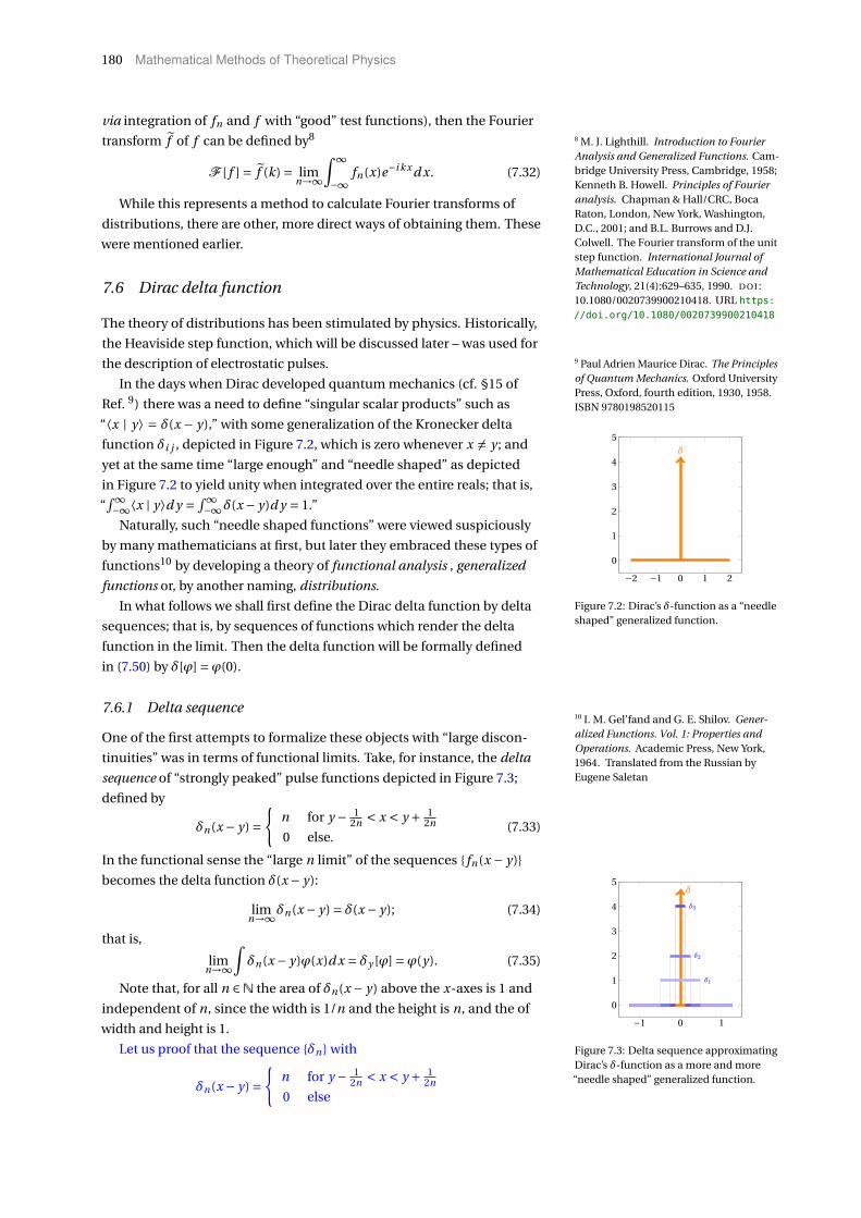
180 Mathematical Methods of Theoretical Physics

via integration of fn and f with “good” test functions), then the Fourier

transform f of f can be defined by8 8 M. J. Lighthill. Introduction to FourierAnalysis and Generalized Functions. Cam-bridge University Press, Cambridge, 1958;Kenneth B. Howell. Principles of Fourieranalysis. Chapman & Hall/CRC, BocaRaton, London, New York, Washington,D.C., 2001; and B.L. Burrows and D.J.Colwell. The Fourier transform of the unitstep function. International Journal ofMathematical Education in Science andTechnology, 21(4):629–635, 1990. D O I :10.1080/0020739900210418. URL https:

//doi.org/10.1080/0020739900210418

F [ f ] = f (k) = limn→∞

∫ ∞

−∞fn(x)e−i kx d x. (7.32)

While this represents a method to calculate Fourier transforms of

distributions, there are other, more direct ways of obtaining them. These

were mentioned earlier.

7.6 Dirac delta function

The theory of distributions has been stimulated by physics. Historically,

the Heaviside step function, which will be discussed later – was used for

the description of electrostatic pulses.

In the days when Dirac developed quantum mechanics (cf. §15 of

Ref. 9) there was a need to define “singular scalar products” such as

9 Paul Adrien Maurice Dirac. The Principlesof Quantum Mechanics. Oxford UniversityPress, Oxford, fourth edition, 1930, 1958.ISBN 9780198520115

“⟨x | y⟩ = δ(x − y),” with some generalization of the Kronecker delta

function δi j , depicted in Figure 7.2, which is zero whenever x 6= y ; and

yet at the same time “large enough” and “needle shaped” as depicted

in Figure 7.2 to yield unity when integrated over the entire reals; that is,

“∫ ∞−∞⟨x | y⟩d y = ∫ ∞

−∞δ(x − y)d y = 1.”

−2 −1 0 1 2

0

1

2

3

4

5δ

Figure 7.2: Dirac’s δ-function as a “needleshaped” generalized function.

Naturally, such “needle shaped functions” were viewed suspiciously

by many mathematicians at first, but later they embraced these types of

functions10 by developing a theory of functional analysis , generalized

10 I. M. Gel’fand and G. E. Shilov. Gener-alized Functions. Vol. 1: Properties andOperations. Academic Press, New York,1964. Translated from the Russian byEugene Saletan

functions or, by another naming, distributions.

In what follows we shall first define the Dirac delta function by delta

sequences; that is, by sequences of functions which render the delta

function in the limit. Then the delta function will be formally defined

in (7.50) by δ[ϕ] =ϕ(0).

7.6.1 Delta sequence

One of the first attempts to formalize these objects with “large discon-

tinuities” was in terms of functional limits. Take, for instance, the delta

sequence of “strongly peaked” pulse functions depicted in Figure 7.3;

defined by

δn(x − y) =

n for y − 12n < x < y + 1

2n

0 else.(7.33)

In the functional sense the “large n limit” of the sequences fn(x − y)

becomes the delta function δ(x − y):

limn→∞δn(x − y) = δ(x − y); (7.34)

that is,

limn→∞

∫δn(x − y)ϕ(x)d x = δy [ϕ] =ϕ(y). (7.35)

−1 0 1

0

1

2

3

4

5δ

δ3

δ2

δ1

Figure 7.3: Delta sequence approximatingDirac’s δ-function as a more and more“needle shaped” generalized function.

Note that, for all n ∈N the area of δn(x − y) above the x-axes is 1 and

independent of n, since the width is 1/n and the height is n, and the of

width and height is 1.

Let us proof that the sequence δn with

δn(x − y) =

n for y − 12n < x < y + 1

2n

0 else

Distributions as generalized functions 181

defined in Equation (7.33) and depicted in Figure 7.3 is a delta sequence;

that is, if, for large n, it converges to δ in a functional sense. In order to

verify this claim, we have to integrate δn(x) with “good” test functions

ϕ(x) and take the limit n →∞; if the result is ϕ(0), then we can identify

δn(x) in this limit with δ(x) (in the functional sense). Since δn(x) is

uniform convergent, we can exchange the limit with the integration; thus

limn→∞

∫ ∞

−∞δn(x − y)ϕ(x)d x

[variable transformation:

x ′ = x − y , x = x ′+ y ,d x ′ = d x,−∞≤ x ′ ≤∞]

= limn→∞

∫ ∞

−∞δn(x ′)ϕ(x ′+ y)d x ′ = lim

n→∞

∫ 12n

− 12n

nϕ(x ′+ y)d x ′

[variable transformation:

u = 2nx ′, x ′ = u

2n,du = 2nd x ′,−1 ≤ u ≤ 1]

= limn→∞

∫ 1

−1nϕ(

u

2n+ y)

du

2n= lim

n→∞1

2

∫ 1

−1ϕ(

u

2n+ y)du

= 1

2

∫ 1

−1lim

n→∞ϕ(u

2n+ y)du = 1

2ϕ(y)

∫ 1

−1du =ϕ(y). (7.36)

Hence, in the functional sense, this limit yields the shifted δ-function δy .

Thus we obtain limn→∞δn[ϕ] = δy [ϕ] =ϕ(y).

Other delta sequences can be ad hoc enumerated as follows. They all

converge towards the delta function in the sense of linear functionals (i.e.

when integrated over a test function).

δn(x) = npπ

e−n2x2, (7.37)

= 1

π

n

1+n2x2 , (7.38)

= 1

π

sin(nx)

x, (7.39)

= = (1∓ i )( n

2π

) 12

e±i nx2(7.40)

= 1

πx

e i nx −e−i nx

2i, (7.41)

= 1

π

ne−x2

1+n2x2 , (7.42)

= 1

2π

∫ n

−ne i xt d t = 1

2πi xe i xt

∣∣∣n

−n, (7.43)

= 1

2π

sin[(

n + 12

)x]

sin( 1

2 x) , (7.44)

= n

π

(sin(nx)

nx

)2

. (7.45)

Other commonly used limit forms of the δ-function are the Gaussian,

Lorentzian, and Dirichlet forms

δε(x) = 1pπε

e−x2

ε2 , (7.46)

= 1

π

ε

x2 +ε2 = 1

2πi

(1

x − iε− 1

x + iε

), (7.47)

= 1

π

sin( xε

)x

, (7.48)

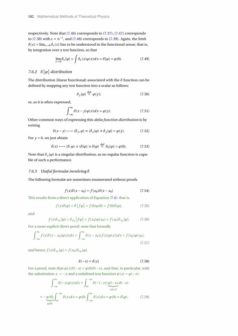
182 Mathematical Methods of Theoretical Physics

respectively. Note that (7.46) corresponds to (7.37), (7.47) corresponds

to (7.38) with ε = n−1, and (7.48) corresponds to (7.39). Again, the limit

δ(x) = limε→0δε(x) has to be understood in the functional sense; that is,

by integration over a test function, so that

limε→0

δε[ϕ] =∫δε(x)ϕ(x)d x = δ[ϕ] =ϕ(0). (7.49)

7.6.2 δ[ϕ

]distribution

The distribution (linear functional) associated with the δ function can be

defined by mapping any test function into a scalar as follows:

δy [ϕ]def= ϕ(y); (7.50)

or, as it is often expressed,∫ ∞

−∞δ(x − y)ϕ(x)d x =ϕ(y). (7.51)

Other common ways of expressing this delta function distribution is by

writing

δ(x − y) ←→⟨δy ,ϕ⟩ ≡ ⟨δy |ϕ⟩ ≡ δy [ϕ] =ϕ(y). (7.52)

For y = 0, we just obtain

δ(x) ←→⟨δ,ϕ⟩ ≡ ⟨δ|ϕ⟩ ≡ δ[ϕ]def= δ0[ϕ] =ϕ(0). (7.53)

Note that δy [ϕ] is a singular distribution, as no regular function is capa-

ble of such a performance.

7.6.3 Useful formulæ involving δ

The following formulæ are sometimes enumerated without proofs.

f (x)δ(x −x0) = f (x0)δ(x −x0) (7.54)

This results from a direct application of Equation (7.4); that is,

f (x)δ[ϕ] = δ[f ϕ

]= f (0)ϕ(0) = f (0)δ[ϕ], (7.55)

and

f (x)δx0 [ϕ] = δx0

[f ϕ

]= f (x0)ϕ(x0) = f (x0)δx0 [ϕ]. (7.56)

For a more explicit direct proof, note that formally∫ ∞

−∞f (x)δ(x −x0)ϕ(x)d x =

∫ ∞

−∞δ(x −x0)( f (x)ϕ(x))d x = f (x0)ϕ(x0),

(7.57)

and hence f (x)δx0 [ϕ] = f (x0)δx0 [ϕ].

δ(−x) = δ(x) (7.58)

For a proof, note that ϕ(x)δ(−x) =ϕ(0)δ(−x), and that, in particular, with

the substitution x →−x and a redefined test function ψ(x) =ϕ(−x):∫ ∞

−∞δ(−x)ϕ(x)d x =

∫ −∞

∞δ(−(−x))ϕ(−x)︸ ︷︷ ︸

=ψ(x)

d(−x)

=−ψ(0)︸︷︷︸ϕ(0)

∫ −∞

∞δ(x)d x =ϕ(0)

∫ ∞

−∞δ(x)d x =ϕ(0) = δ[ϕ]. (7.59)

Distributions as generalized functions 183

For the δ distribution with its “extreme concentration” at the origin,

a “nonconcentrated test function” suffices; in particular, a constant

“test” function – even without compact support and sufficiently strong

damping at infinity – such as ϕ(x) = 1 is fine. This is the reason why test

functions need not show up explicitly in expressions, and, in particular,

integrals, containing δ. Because, say, for suitable functions g (x) “well

behaved” at the origin, formally by invoking (7.54)∫ ∞

−∞g (x)δ(x − y)d x =

∫ ∞

−∞g (y)δ(x − y)d x

= g (y)∫ ∞

−∞δ(x − y)d x = g (y). (7.60)

xδ(x) = 0 (7.61)

For a proof invoke (7.54), or explicitly consider

xδ[ϕ] = δ[xϕ

]= 0ϕ(0) = 0. (7.62)

For a 6= 0,

δ(ax) = 1

|a|δ(x), (7.63)

and, more generally,

δ(a(x −x0)) = 1

|a|δ(x −x0) (7.64)

For the sake of a proof, consider the case a > 0 as well as x0 = 0 first:∫ ∞

−∞δ(ax)ϕ(x)d x

[variable substitution y = ax, x = y

a,d x = 1

ad y]

= 1

a

∫ ∞

−∞δ(y)ϕ

( y

a

)d y

= 1

aϕ(0) = 1

|a|ϕ(0); (7.65)

and, second, the case a < 0: ∫ ∞

−∞δ(ax)ϕ(x)d x

[variable substitution y = ax, x = y

a,d x = 1

ad y]

= 1

a

∫ −∞

∞δ(y)ϕ

( y

a

)d y

=− 1

a

∫ ∞

−∞δ(y)ϕ

( y

a

)d y

=− 1

aϕ(0) = 1

|a|ϕ(0). (7.66)

In the case of x0 6= 0 and ±a > 0, we obtain∫ ∞

−∞δ(a(x −x0))ϕ(x)d x

[variable substitution y = a(x −x0), x = y

a+x0,d x = 1

ad y]

=± 1

a

∫ ∞

−∞δ(y)ϕ

( y

a+x0

)d y

=± 1

aϕ(0) = 1

|a|ϕ(x0). (7.67)

184 Mathematical Methods of Theoretical Physics

If there exists a simple singularity x0 of f (x) in the integration interval,

then

δ( f (x)) = 1

| f ′(x0)|δ(x −x0). (7.68)

More generally, if f has only simple roots and f ′ is nonzero there,

δ( f (x)) =∑xi

δ(x −xi )

| f ′(xi )| (7.69)

where the sum extends over all simple roots xi in the integration interval.

In particular,

δ(x2 −x20) = 1

2|x0|[δ(x −x0)+δ(x +x0)] (7.70)

For a sloppy proof, note that since f has only simple roots, it can be An example is a polynomial of degree k ofthe form f = A

∏ki=1(x −xi ); with mutually

distinct xi , 1 ≤ i ≤ k.expanded around these roots as

Again the symbol “O” stands for “of theorder of” or “absolutely bound by” inthe following way: if g (x) is a positivefunction, then f (x) =O(g (x)) implies thatthere exist a positive real number m suchthat | f (x)| < mg (x).

f (x) = f (x0)︸ ︷︷ ︸=0

+(x −x0) f ′(x0)+O((x −x0)2)

= (x −x0)[

f ′(x0)+O (|x −x0|)]≈ (x −x0) f ′(x0),

with nonzero f ′(x0) ∈ R. By identifying f ′(x0) with a in Equation (7.63) The simplest nontrivial case is f (x) =a +bx = b

(ab +x

), for which x0 =− a

b and

f ′(x0 = a

b

)= b.

we obtain Equation (7.69).

For a proof11 the integration which originally extend over the set of11 Sergio Ferreira Cortizo. On Dirac’s deltacalculus, 1995. URL https://arxiv.org/

abs/funct-an/9510004

real numbers R can be reduced to intervals [xi − ri , xi + ri ], containing

the roots xi of f (x). so that the “radii” ri are “small enough” for these

intervals to be pairwise disjoint, and f (x) 6= 0 for any x outside of the

union set of these intervals. Therefore the integration over the entire reals

can be reduced to the sum of the integrations over the intervals; that is,

∫ +∞

−∞δ( f (x))ϕ(x)d x =∑

i

∫ xi+ri

xi−ri

δ( f (x))ϕ(x)d x. (7.71)

The terms in the sum can be evaluated separately; so let us concen-

trate on the i ’th term∫ xi+ri

xi−riδ( f (x))ϕ(x)d x in (7.71). Restriction to a

sufficiently small single region [xi − ri , xi + ri ], and the assumption of

simple roots guarantees that f (x) is invertible within that region; with the

inverse f −1i ; that is,

f −1i ( f (x)) = x for x ∈ [xi − ri , xi + ri ]; (7.72)

and, in particular, f (xi ) = 0 and f −1i (0) = f −1

i ( f (xi )) = xi . Furthermore,

this inverse f −1i is monotonic, differentiable and its derivative is nonzero

within [ f (xi − ri ), f (xi + ri )]. Define

y = f (x),

x = f −1i (y), and

d y = f ′(x)d x, or d x = d y

f ′(x), (7.73)

Distributions as generalized functions 185

so that, for f ′(xi ) > 0,∫ xi+ri

xi−ri

δ( f (x))ϕ(x)d x =∫ xi+ri

xi−ri

δ( f (x))ϕ(x)

f ′(x)f ′(x)d x

=∫ f (xi+ri )

f (xi−ri )δ(y)

ϕ( f −1i (y))

f ′( f −1i (y))

d y

= ϕ( f −1i (0))

f ′( f −1i (0))

= ϕ( f −1i ( f (xi )))

f ′( f −1i ( f (xi )))

= ϕ(xi )

f ′(xi ). (7.74)

Likewise, for f ′(xi ) < 0,∫ xi+ri

xi−ri

δ( f (x))ϕ(x)d x =∫ xi+ri

xi−ri

δ( f (x))ϕ(x)

f ′(x)f ′(x)d x

=∫ f (xi+ri )

f (xi−ri )δ(y)

ϕ( f −1i (y))

f ′( f −1i (y))

d y =−∫ f (xi−ri )

f (xi+ri )δ(y)

ϕ( f −1i (y))

f ′( f −1i (y))

d y

=− ϕ( f −1i (0))

f ′( f −1i (0))

=− ϕ( f −1i ( f (xi )))

f ′( f −1i ( f (xi )))

=− ϕ(xi )

f ′(xi ). (7.75)

|x|δ(x2) = δ(x) (7.76)

For a proof consider

|x|δ(x2)[ϕ] =∫ ∞

−∞|x|δ(x2)ϕ(x)d x

= lima→0+

∫ ∞

−∞|x|δ(x2 −a2)ϕ(x)d x

= lima→0+

∫ ∞

−∞|x|2a

[δ(x −a)+δ(x +a)]ϕ(x)d x

= lima→0+

[∫ ∞

−∞|x|2a

δ(x −a)ϕ(x)d x +∫ ∞

−∞|x|2a

δ(x +a)ϕ(x)d x

]= lim

a→0+

[ |a|2a

ϕ(a)+ |−a|2a

ϕ(−a)

]= lim

a→0+

[1

2ϕ(a)+ 1

2ϕ(−a)

]= 1

2ϕ(0)+ 1

2ϕ(0) =ϕ(0) = δ[ϕ]. (7.77)

−xδ′(x) = δ(x), (7.78)

which is a direct consequence of Equation (7.31). More explicitly, we can

use partial integration and obtain

−∫ ∞

−∞xδ′(x)ϕ(x)d x

=− xδ(x)|∞−∞+∫ ∞

−∞δ(x)

d

d x

(xϕ(x)

)d x

=∫ ∞

−∞δ(x)xϕ′(x)d x +

∫ ∞

−∞δ(x)ϕ(x)d x

= 0ϕ′(0)+ϕ(0) =ϕ(0). (7.79)

δ(n)(−x) = (−1)nδ(n)(x), (7.80)

186 Mathematical Methods of Theoretical Physics

where the index (n) denotes n-fold differentiation, can be proven by

[recall that, by the chain rule of differentiation, dd xϕ(−x) =−ϕ′(−x)]∫ ∞

−∞δ(n)(−x)ϕ(x)d x

[variable substitution x →−x]

=−∫ −∞

∞δ(n)(x)ϕ(−x)d x =

∫ ∞

−∞δ(n)(x)ϕ(−x)d x

= (−1)n∫ ∞

−∞δ(x)

[d n

d xn ϕ(−x)

]d x

= (−1)n∫ ∞

−∞δ(x)

[(−1)nϕ(n)(−x)

]d x

=∫ −∞

∞δ(x)ϕ(n)(−x)d x

[variable substitution x →−x]

=−∫ −∞

∞δ(−x)ϕ(n)(x)d x =

∫ ∞

−∞δ(x)ϕ(n)(x)d x

= (−1)n∫ −∞

∞δ(n)(x)ϕ(x)d x. (7.81)

Because of an additional factor (−1)n from the chain rule, in particular,

from the n-fold “inner” differentiation of −x, follows that

d n

d xn δ(−x) = (−1)nδ(n)(−x) = δ(n)(x). (7.82)

xm+1δ(m)(x) = 0, (7.83)

where the index (m) denotes m-fold differentiation;

x2δ′(x) = 0, (7.84)

which is a consequence of Equation (7.31). More generally, formally,

xnδ(m)(x) = (−1)nn!δnmδ(x), or

xnδ(m)[ϕ] = (−1)nn!δnmδ[ϕ]. (7.85)

This can be demonstrated by considering

xnδ(m)[ϕ] =∫ ∞

−∞xnδ(m)(x)ϕ(x)d x =

∫ ∞

−∞δ(m)(x)xnϕ(x)d x

= (−1)m∫ ∞

−∞δ(x)

d m

d xm

[xnϕ(x)

]d x = (−1)m d m

d xm

[xnϕ(x)

]∣∣∣∣x=0

[after n derivations the only remaining nonvanishing term

is of degree n = m, with xmϕ(x) resulting in m!ϕ(0)]

= (−1)mm!δnmϕ(0) = (−1)nn!δnmδ[ϕ]. (7.86)

A shorter proof employing the polynomial xn as a “test” function may

also be enumerated by

⟨xnδ(m)|1⟩ = ⟨δ(m)|xn⟩ = (−1)n⟨δ| d m

d xm xn⟩= (−1)nn!δnm ⟨δ|1⟩︸ ︷︷ ︸

1

. (7.87)

Distributions as generalized functions 187

Suppose H is the Heaviside step function as defined later in Equa-

tion (7.122), then

H ′[ϕ] = δ[ϕ]. (7.88)

For a proof, note that

H ′[ϕ] = d

d xH [ϕ] =−H [ϕ′] =−

∫ ∞

−∞H(x)ϕ′(x)d x

=−∫ ∞

0ϕ′(x)d x =− ϕ(x)

∣∣x=∞x=0 =−ϕ(∞)︸ ︷︷ ︸

=0

+ϕ(0) =ϕ(0) = δ[ϕ]. (7.89)

d 2

d x2 [xH(x)] = d

d x[H(x)+xδ(x)︸ ︷︷ ︸

0

] = d

d xH(x) = δ(x) (7.90)

If δ(3)(r) = δ(x)δ(y)δ(r ) with r = (x, y , z) and |r| = r , then

δ(3)(r) = δ(x)δ(y)δ(z) =− 1

4π∆

1

r(7.91)

δ(3)(r) =− 1

4π(∆+k2)

e i kr

r=− 1

4π(∆+k2)

coskr

r, (7.92)

and therefore

(∆+k2)sinkr

r= 0. (7.93)

In quantum field theory, phase space integrals of the form

1

2E=

∫d p0 H(p0)δ(p2 −m2) (7.94)

with E = (~p2 +m2)(1/2) are exploited.

For a proof consider∫ ∞

−∞H(p0)δ(p2 −m2)d p0 =

∫ ∞

−∞H(p0)δ

((p0)2 −p2 −m2)d p0

=∫ ∞

−∞H(p0)δ

((p0)2 −E 2)d p0

=∫ ∞

−∞H(p0)

1

2E

[δ

(p0 −E

)+δ(p0 +E

)]d p0

= 1

2E

∫ ∞

−∞

[H(p0)δ

(p0 −E

)︸ ︷︷ ︸=δ(p0−E)

+H(p0)δ(p0 +E

)︸ ︷︷ ︸=0

]d p0

= 1

2E

∫ ∞

−∞δ

(p0 −E

)d p0︸ ︷︷ ︸

=1

= 1

2E. (7.95)

7.6.4 Fourier transform of δ

The Fourier transform of the δ-function can be obtained straightfor-

wardly by insertion into Equation (6.19);12 that is, with A = B = 1

12 The convention A = B = 1 differs fromthe convention A = 2π and B = 1 usedearlier in Section 7.3.4, page 178. A and Brefer to Equation (6.19), page 167.

188 Mathematical Methods of Theoretical Physics

F [δ(x)] = δ(k) =∫ ∞

−∞δ(x)e−i kx d x

= e−i 0k∫ ∞

−∞δ(x)d x

= 1, and thus

F−1[δ(k)] =F−1[1] = δ(x)

= 1

2π

∫ ∞

−∞e i kx dk

= 1

2π

∫ ∞

−∞[cos(kx)+ i sin(kx)]dk

= 1

π

∫ ∞

0cos(kx)dk + i

2π

∫ ∞

−∞sin(kx)dk

= 1

π

∫ ∞

0cos(kx)dk. (7.96)

That is, the Fourier transform of the δ-function is just a constant. δ-

spiked signals carry all frequencies in them. Note also that F [δy ] =F [δ(y −x)] = e i k yF [δ(x)] = e i k yF [δ].

From Equation (7.96 ) we can compute

F [1] = 1(k) =∫ ∞

−∞e−i kx d x

[variable substitution x →−x]

=∫ −∞

+∞e−i k(−x)d(−x)

=−∫ −∞

+∞e i kx d x

=∫ +∞

−∞e i kx d x

= 2πδ(k). (7.97)

7.6.5 Eigenfunction expansion of δ

The δ-function can be expressed in terms of, or “decomposed” into,

various eigenfunction expansions. We mention without proof13 that, for 13 Dean G. Duffy. Green’s Functions withApplications. Chapman and Hall/CRC,Boca Raton, 2001

0 < x, x0 < L, two such expansions in terms of trigonometric functions are

δ(x −x0) = 2

L

∞∑k=1

sin

(πkx0

L

)sin

(πkx

L

)= 1

L+ 2

L

∞∑k=1

cos

(πkx0

L

)cos

(πkx

L

). (7.98)

This “decomposition of unity” is analogous to the expansion of the

identity in terms of orthogonal projectors Ei (for one-dimensional

projectors, Ei = |i ⟩⟨i |) encountered in the spectral theorem 1.27.1.

Other decomposions are in terms of orthonormal (Legendre) poly-

nomials (cf. Sect. 11.6 on page 256), or other functions of mathematical

physics discussed later.

7.6.6 Delta function expansion

Just like “slowly varying” functions can be expanded into a Taylor series

in terms of the power functions xn , highly localized functions can be

Distributions as generalized functions 189

expanded in terms of derivatives of the δ-function in the form14 14 Ismo V. Lindell. Delta function ex-pansions, complex delta functions andthe steepest descent method. Ameri-can Journal of Physics, 61(5):438–442,1993. D O I : 10.1119/1.17238. URLhttps://doi.org/10.1119/1.17238

f (x) ∼ f0δ(x)+ f1δ′(x)+ f2δ

′′(x)+·· ·+ fnδ(n)(x)+·· · =

∞∑k=1

fkδ(k)(x),

with fk = (−1)k

k!

∫ ∞

−∞f (y)yk d y .

(7.99)

The sign “∼” denotes the functional character of this “equation” (7.99).

The delta expansion (7.99) can be proven by considering a smooth

function g (x), and integrating over its expansion; that is,∫ ∞

−∞f (x)ϕ(x)d x

=∫ ∞

−∞[

f0δ(x)+ f1δ′(x)+ f2δ

′′(x)+·· ·+ fnδ(n)(x)+·· ·]ϕ(x)d x

= f0ϕ(0)− f1ϕ′(0)+ f2ϕ

′′(0)+·· ·+ (−1)n fnϕ(n)(0)+·· · , (7.100)

and comparing the coefficients in (7.100) with the coefficients of the

Taylor series expansion of ϕ at x = 0∫ ∞

−∞ϕ(x) f (x) =

∫ ∞

−∞

[ϕ(0)+xϕ′(0)+·· ·+ xn

n!ϕ(n)(0)+·· ·

]f (x)d x

=ϕ(0)∫ ∞

−∞f (x)d x +ϕ′(0)

∫ ∞

−∞x f (x)d x +·· ·+ϕ(n)(0)

∫ ∞

−∞xn

n!f (x)d x︸ ︷︷ ︸

(−1)n fn

+·· · ,

(7.101)

so that fn = (−1)n∫ ∞−∞

xn

n! f (x)d x.

7.7 Cauchy principal value

7.7.1 Definition

The (Cauchy) principal value P (sometimes also denoted by p.v.) is a

value associated with an integral as follows: suppose f (x) is not locally

integrable around c; then

P

∫ b

af (x)d x = lim

ε→0+

[∫ c−ε

af (x)d x +

∫ b

c+εf (x)d x

]= limε→0+

∫[a,c−ε]∪[c+ε,b]

f (x)d x. (7.102)

For example, the integral∫ 1−1

d xx diverges, but

P

∫ 1

−1

d x

x= limε→0+

[∫ −ε

−1

d x

x+

∫ 1

+εd x

x

][variable substitution x →−x in the first integral]

= limε→0+

[∫ +ε

+1

d x

x+

∫ 1

+εd x

x

]= limε→0+

[logε− log1+ log1− logε

]= 0. (7.103)

190 Mathematical Methods of Theoretical Physics

7.7.2 Principle value and pole function 1x distribution

The “standalone function” 1x does not define a distribution since it is

not integrable in the vicinity of x = 0. This issue can be “alleviated” or

“circumvented” by considering the principle value P 1x . In this way the

principle value can be transferred to the context of distributions by

defining a principal value distribution in a functional sense:

P

(1

x

)[ϕ

]= limε→0+

∫|x|>ε

1

xϕ(x)d x

= limε→0+

[∫ −ε

−∞1

xϕ(x)d x +

∫ ∞

+ε1

xϕ(x)d x

][variable substitution x →−x in the first integral]

= limε→0+

[∫ +ε

+∞1

xϕ(−x)d x +

∫ ∞

+ε1

xϕ(x)d x

]= limε→0+

[−

∫ ∞

+ε1

xϕ(−x)d x +

∫ ∞

+ε1

xϕ(x)d x

]= limε→0+

∫ +∞

ε

ϕ(x)−ϕ(−x)

xd x

=∫ +∞

0

ϕ(x)−ϕ(−x)

xd x. (7.104)

7.8 Absolute value distribution

The distribution associated with the absolute value |x| is defined by

|x|[ϕ]= ∫ ∞

−∞|x|ϕ(x)d x. (7.105)

|x|[ϕ]can be evaluated and represented as follows:

|x|[ϕ]= ∫ ∞

−∞|x|ϕ(x)d x

=∫ 0

−∞(−x)ϕ(x)d x +

∫ ∞

0xϕ(x)d x =−

∫ 0

−∞xϕ(x)d x +

∫ ∞

0xϕ(x)d x

[variable substitution x →−x,d x →−d x in the first integral]

=−∫ 0

+∞xϕ(−x)d x +

∫ ∞

0xϕ(x)d x =

∫ ∞

0xϕ(−x)d x +

∫ ∞

0xϕ(x)d x

=∫ ∞

0x

[ϕ(x)+ϕ(−x)

]d x.

(7.106)

An alternative derivation uses the reflection symmetry at zero:

|x|[ϕ]= ∫ ∞

−∞|x|ϕ(x)d x =

∫ ∞

−∞|x|2

[ϕ(x)+ϕ(−x)

]d x

=∫ ∞

0x

[ϕ(x)+ϕ(−x)

]d x. (7.107)

Distributions as generalized functions 191

7.9 Logarithm distribution

7.9.1 Definition

Let, for x 6= 0,

log |x|[ϕ]= ∫ ∞

−∞log |x|ϕ(x)d x

=∫ 0

−∞log(−x)ϕ(x)d x +

∫ ∞

0log xϕ(x)d x

[variable substitution x →−x,d x →−d x in the first integral]

=∫ 0

+∞log(−(−x))ϕ(−x)d(−x)+

∫ ∞

0log xϕ(x)d x

=−∫ 0

+∞log xϕ(−x)d x +

∫ ∞

0log xϕ(x)d x

=∫ ∞

0log xϕ(−x)d x +

∫ ∞

0log xϕ(x)d x

=∫ ∞

0log x

[ϕ(x)+ϕ(−x)

]d x. (7.108)

7.9.2 Connection with pole function

Note that

P

(1

x

)[ϕ

]= d

d xlog |x|[ϕ]

, (7.109)

and thus, for the principal value of a pole of degree n,

P

(1

xn

)[ϕ

]= (−1)n−1

(n −1)!d n

d xn log |x|[ϕ]. (7.110)

For a proof of Equation (7.109) consider the functional derivative

log′ |x|[ϕ] by insertion into Equation (7.108); as well as by using the

symmetry of the resulting integral kernel at zero: Note that, for x < 0, dd x log |x| =

dd x log(−x) =

[d

d y log(y)]

y=−xd

d x (−x) =−1−x = 1

x .log′ |x|[ϕ] =− log |x|[ϕ′] =−∫ ∞

−∞log |x|ϕ′(x)d x

=−1

2

∫ ∞

−∞log |x|[ϕ′(x)+ϕ′(−x)

]d x

=−1

2

∫ ∞

−∞log |x| d

d x

[ϕ(x)−ϕ(−x)

]d x

= 1

2

∫ ∞

−∞

(d

d xlog |x|

)[ϕ(x)−ϕ(−x)

]d x

= 1

2

∫ 0

−∞

[d

d xlog(−x)

][ϕ(x)−ϕ(−x)

]d x+

+∫ ∞

0

(d

d xlog x

)[ϕ(x)−ϕ(−x)

]d x

= 1

2

∫ 0

∞

(d

d xlog x

)[ϕ(−x)−ϕ(x)

]d x+

+∫ ∞

0

(d

d xlog x

)[ϕ(x)−ϕ(−x)

]d x

=

∫ ∞

0

1

x

[ϕ(x)−ϕ(−x)

]d x =P

(1

x

)[ϕ

], (7.111)

The more general Equation (7.110) follows by direct differentiation.

192 Mathematical Methods of Theoretical Physics

7.10 Pole function 1xn distribution

For n ≥ 2, the integral over 1xn is undefined even if we take the principal

value. Hence the direct route to an evaluation is blocked, and we have to

take an indirect approach via derivatives of15 1x . Thus, let 15 Thomas Sommer. Verallgemein-

erte Funktionen, 2012. unpublishedmanuscript1

x2

[ϕ

]=− d

d x

1

x

[ϕ

]= 1

x

[ϕ′]= ∫ ∞

0

1

x

[ϕ′(x)−ϕ′(−x)

]d x

=P

(1

x

)[ϕ′] . (7.112)

Also,

1

x3

[ϕ

]=−1

2

d

d x

1

x2

[ϕ

]= 1

2

1

x2

[ϕ′]= 1

2x

[ϕ′′]

= 1

2

∫ ∞

0

1

x

[ϕ′′(x)−ϕ′′(−x)

]d x

= 1

2P

(1

x

)[ϕ′′] . (7.113)

More generally, for n > 1, by induction, using (7.112) as induction

basis,

1

xn

[ϕ

]=− 1

n −1

d

d x

1

xn−1

[ϕ

]= 1

n −1

1

xn−1

[ϕ′]

=−(

1

n −1

)(1

n −2

)d

d x

1

xn−2

[ϕ′]= 1

(n −1)(n −2)

1

xn−2

[ϕ′′]

= ·· · = 1

(n −1)!1

x

[ϕ(n−1)]

= 1

(n −1)!

∫ ∞

0

1

x

[ϕ(n−1)(x)−ϕ(n−1)(−x)

]d x

= 1

(n −1)!P

(1

x

)[ϕ(n−1)] . (7.114)

7.11 Pole function 1x±iα distribution

We are interested in the limit α→ 0 of 1x+iα . Let α> 0. Then,

1

x + iα

[ϕ

]= ∫ ∞

−∞1

x + iαϕ(x)d x

=∫ ∞

−∞x − iα

(x + iα)(x − iα)ϕ(x)d x

=∫ ∞

−∞x − iα

x2 +α2ϕ(x)d x

=∫ ∞

−∞x

x2 +α2ϕ(x)d x − iα∫ ∞

−∞1

x2 +α2ϕ(x)d x. (7.115)

Let us treat the two summands of (7.115) separately. (i) Upon variable

substitution x =αy , d x =αd y in the second integral in (7.115) we obtain

α

∫ ∞

−∞1

x2 +α2ϕ(x)d x =α∫ ∞

−∞1

α2 y2 +α2ϕ(αy)αd y

=α2∫ ∞

−∞1

α2(y2 +1)ϕ(αy)d y

=∫ ∞

−∞1

y2 +1ϕ(αy)d y (7.116)

Distributions as generalized functions 193

In the limit α→ 0, this is

limα→0

∫ ∞

−∞1

y2 +1ϕ(αy)d y =ϕ(0)

∫ ∞

−∞1

y2 +1d y

=ϕ(0)(arctan y

)∣∣y=∞y=−∞

=πϕ(0) =πδ[ϕ]. (7.117)

(ii) The first integral in (7.115) is ∫ ∞

−∞x

x2 +α2ϕ(x)d x

=∫ 0

−∞x

x2 +α2ϕ(x)d x +∫ ∞

0

x

x2 +α2ϕ(x)d x

=∫ 0

+∞−x

(−x)2 +α2ϕ(−x)d(−x)+∫ ∞

0

x

x2 +α2ϕ(x)d x

=−∫ ∞

0

x

x2 +α2ϕ(−x)d x +∫ ∞

0

x

x2 +α2ϕ(x)d x

=∫ ∞

0

x

x2 +α2

[ϕ(x)−ϕ(−x)

]d x. (7.118)

In the limit α→ 0, this becomes

limα→0

∫ ∞

0

x

x2 +α2

[ϕ(x)−ϕ(−x)

]d x =

∫ ∞

0

ϕ(x)−ϕ(−x)

xd x

P

(1

x

)[ϕ

], (7.119)

where in the last step the principle value distribution (7.104) has been

used.

Putting all parts together, we obtain

1

x + i 0+[ϕ

]= limα→0+

1

x + iα

[ϕ

]=P

(1

x

)[ϕ

]− iπδ[ϕ] =P

(1

x

)− iπδ

[ϕ].

(7.120)

A very similar calculation yields

1

x − i 0+[ϕ

]= limα→0+

1

x − iα

[ϕ

]=P

(1

x

)[ϕ

]+ iπδ[ϕ] =P

(1

x

)+ iπδ

[ϕ].

(7.121)

These equations (7.120) and (7.121) are often called the Sokhotsky

formula, also known as the Plemelj formula, or the Plemelj-Sokhotsky

formula.16

16 Yu. V. Sokhotskii. On definite integralsand functions used in series expansions.PhD thesis, St. Petersburg, 1873; andJosip Plemelj. Ein Ergänzungssatzzur Cauchyschen Integraldarstellunganalytischer Funktionen, Randwertebetreffend. Monatshefte für Mathematikund Physik, 19(1):205–210, Dec 1908. ISSN1436-5081. D O I : 10.1007/BF01736696.URL https://doi.org/10.1007/

BF01736696

7.12 Heaviside or unit step function

7.12.1 Ambiguities in definition

Let us now turn to Heaviside’s electromagnetic pulse function, often re-

ferred to as Heaviside’s unit step function. One of the possible definitions

of the Heaviside step function H(x), and maybe the most common one

– they differ by the difference of the value(s) of H(0) at the origin x = 0, a

difference which is irrelevant measure theoretically for “good” functions

since it is only about an isolated point – is

H(x −x0) =

1 for x ≥ x0

0 for x < x0(7.122)

194 Mathematical Methods of Theoretical Physics

Alternatively one may define H(0) = 12 , as plotted in Figure 7.4.

H(x −x0) = 1

2+ 1

πlimε→0+

arctan( x −x0

ε

)=

1 for x > x012 for x = x0

0 for x < x0

(7.123)

and, since this affects only an isolated point at x = x0, we may happily do

so if we prefer.

−2 −1 1 2

0.5

1

0

Figure 7.4: Plot of the Heaviside stepfunction H(x). Its value at x = 0 dependson its definition.

It is also very common to define the unit step function as the an-

tiderivative of the δ function; likewise the delta function is the derivative

of the Heaviside step function; that is,

H ′[ϕ] = δ[ϕ], or formally,

H(x −x0) =∫ x−x0

−∞δ(t )d t , and

d

d xH(x −x0) = δ(x −x0). (7.124)

The latter equation can, in the functional sense – that is, by integration

over a test function – be proven by

H ′[ϕ] = ⟨H ′,ϕ⟩ =−⟨H ,ϕ′⟩ =−∫ ∞

−∞H(x)ϕ′(x)d x

=−∫ ∞

0ϕ′(x)d x =− ϕ(x)

∣∣x=∞x=0

=−ϕ(∞)︸ ︷︷ ︸=0

+ϕ(0) = ⟨δ,ϕ⟩ = δ[ϕ] (7.125)

for all test functions ϕ(x). Hence we can – in the functional sense –

identify δ with H ′. More explicitly, through integration by parts, we

obtain ∫ ∞

−∞

[d

d xH(x −x0)

]ϕ(x)d x

= H(x −x0)ϕ(x)∣∣∞−∞−

∫ ∞

−∞H(x −x0)

[d

d xϕ(x)

]d x

= H(∞)︸ ︷︷ ︸=1

ϕ(∞)︸ ︷︷ ︸=0

−H(−∞)︸ ︷︷ ︸=0

ϕ(−∞)︸ ︷︷ ︸=0

−∫ ∞

x0

[d

d xϕ(x)

]d x

=−∫ ∞

x0

[d

d xϕ(x)

]d x

=− ϕ(x)∣∣x=∞

x=x0=−[ϕ(∞)︸ ︷︷ ︸

=0

−ϕ(x0)] =ϕ(x0). (7.126)

7.12.2 Unit step function sequenceFor a great variety of unit step functionsequences see http://mathworld.wolfram.com/HeavisideStepFunction.

html.

As mentioned earlier, a commonly used limit form of the Heaviside step

function is

H(x) = limε→0

Hε(x) = limε→0

[1

2+ 1

πarctan

( x

ε

)]. (7.127)

respectively.

Another limit representation of the Heaviside function is in terms of

the Dirichlet’s discontinuity factor as follows:

H(x) = limt→∞Ht (x)

= 1

2+ 1

πlim

t→∞

∫ t

0

sin(kx)

kdk

= 1

2+ 1

π

∫ ∞

0

sin(kx)

kdk. (7.128)

Distributions as generalized functions 195

A proof17 uses a variant of the sine integral function 17 Eli Maor. Trigonometric Delights.Princeton University Press, Princeton,1998. URL http://press.princeton.

edu/books/maor/Si(y) =

∫ y

0

sin t

td t (7.129)

which in the limit of large argument y converges towards the Dirichlet

integral (no proof is given here)

limy→∞Si(y) =

∫ ∞

0

sin t

td t = π

2. (7.130)

Suppose we replace t with t = kx in the Dirichlet integral (7.130),

whereby x 6= 0 is a nonzero constant; that is,∫ ∞

0

sin(kx)

kxd(kx) = H(x)

∫ ∞

0

sin(kx)

kdk +H(−x)

∫ −∞

0

sin(kx)

kdk.

(7.131)

Note that the integration border ±∞ changes, depending on whether x is

positive or negative, respectively.

If x is positive, we leave the integral (7.131) as is, and we recover the

original Dirichlet integral (7.130), which is π2 . If x is negative, in order to

recover the original Dirichlet integral form with the upper limit ∞, we

have to perform yet another substitution k →−k on (7.131), resulting in

=∫ −∞

0

sin(−kx)

−kd(−k) =−

∫ ∞

0

sin(kx)

kdk =−Si(∞) =−π

2, (7.132)

since the sine function is an odd function; that is, sin(−ϕ) =−sinϕ.

The Dirichlet’s discontinuity factor (7.128) is obtained by normalizing

the absolute value of (7.131) [and thus also (7.132)] to 12 by multiplying it

with 1/π, and by adding 12 .

7.12.3 Useful formulæ involving H

Some other formulæ involving the unit step function are

H(−x) = 1−H(x), or H(x) = 1−H(−x), (7.133)

H(αx) =H(x) for real α> 0,

1−H(x) for real α< 0,(7.134)

H(x) = 1

2+

∞∑l=0

(−1)l (2l )!(4l +3)

22l+2l !(l +1)!P2l+1(x), (7.135)

where P2l+1(x) is a Legendre polynomial. Furthermore,

δ(x) = limε→0+

1

εH

(ε2−|x|

). (7.136)

The latter equation can be proven by

limε→0+

∫ ∞

−∞1

εH

(ε2−|x|

)ϕ(x)d x = lim

ε→0+1

ε

∫ ε2

− ε2

ϕ(x)d x

[mean value theorem: ∃ y with −ε2≤ y ≤ ε

2such that]

= limε→0+

1

εϕ(y)

∫ ε2

− ε2

d x︸ ︷︷ ︸=ε

= limε→0+

ϕ(y) =ϕ(0) = δ[ϕ]. (7.137)

A Fourier integral representation (7.142) of H(x) derived later is18

18 The second integral is the complexconjugate of the first integral, ab = ab,

and[

1k−iε

]=

[k+iε

(k+iε)(k−iε)

]= k−iε

k+ε2 =k−iε

(k+iε)(k−iε) = 1k+iε .H(x) = lim

ε→0+1

2πi

∫ ∞

−∞1

t − iεe i xt d t = lim

ε→0+−1

2πi

∫ ∞

−∞1

t + iεe−i xt d t . (7.138)

196 Mathematical Methods of Theoretical Physics

7.12.4 H[ϕ

]distribution

The distribution associated with the Heaviside function H(x) is defined

by

H[ϕ

]= ∫ ∞

−∞H(x)ϕ(x)d x. (7.139)

H[ϕ

]can be evaluated and represented as follows:

H[ϕ

]= ∫ 0

−∞H(x)︸ ︷︷ ︸=0

ϕ(x)d x +∫ ∞

0H(x)︸ ︷︷ ︸=1

ϕ(x)d x =∫ ∞

0ϕ(x)d x. (7.140)

Recall that, as has been pointed out in Equations (7.88) and (7.89),

H[ϕ

]is the antiderivative of the delta function; that is, H ′ [ϕ]= δ[

ϕ].

7.12.5 Regularized unit step function

In order to be able to define the Fourier transformation associated with

the Heaviside function we sometimes consider the distribution of the

regularized Heaviside function

Hε(x) = H(x)e−εx , (7.141)

with ε> 0, such that limε→0+ Hε(x) = H(x).

7.12.6 Fourier transform of the unit step function

The Fourier transform19 of the Heaviside (unit step) function cannot be 19 The convention A = B = 1 is used. A andB refer to Equation (6.19), page 167.directly obtained by insertion into Equation (6.19) because the associ-

ated integrals do not exist. We shall thus use the regularized Heaviside

function (7.141), and arrive at Sokhotsky’s formula (also known as the

Plemelj’s formula, or the Plemelj-Sokhotsky formula)

F [H(x)] = H(k) =∫ ∞

−∞H(x)e−i kx d x

=πδ(k)− iP1

k

=−i

(iπδ(k)+P

1

k

)= limε→0+

− i

k − iε(7.142)

We shall compute the Fourier transform of the regularized Heaviside

function Hε(x) = H(x)e−εx , with ε> 0, of Equation (7.141); that is,20

20 Thomas Sommer. Verallgemein-erte Funktionen, 2012. unpublishedmanuscript

Distributions as generalized functions 197

F [Hε(x)] =F [H(x)e−εx ] = Hε(k)

=∫ ∞

−∞Hε(x)e−i kx d x

=∫ ∞

−∞H(x)e−εx e−i kx d x

=∫ ∞

−∞H(x)e−i kx+(−i )2εx d x

=∫ ∞

−∞H(x)e−i (k−iε)x d x

=∫ ∞

0e−i (k−iε)x d x

=[−e−i (k−iε)x

i (k − iε)

]∣∣∣∣∣x=∞

x=0

=[−e−i k e−εx

i (k − iε)

]∣∣∣∣∣x=∞

x=0

=[−e−i k∞e−ε∞

i (k − iε)

]−

[−e−i k0e−ε0

i (k − iε)

]

= 0− (−1)

i (k − iε)=− i

k − iε=−i

[P

(1

k

)+ iπδ(k)

]. (7.143)

where in the last step Sokhotsky’s formula (7.121) has been used. We

therefore conclude that

F [H(x)] =F [H0+ (x)] = limε→0+

F [Hε(x)] =πδ(k)− iP

(1

k

). (7.144)

7.13 The sign function

7.13.1 Definition

The sign function is defined by

sgn(x −x0) = limε→0+

2

πarctan

( x −x0

ε

)=

−1 for x < x0

0 for x = x0

+1 for x > x0

. (7.145)

It is plotted in Figure 7.5. −2 −1 1 2

1

0

−1

Figure 7.5: Plot of the sign function.

7.13.2 Connection to the Heaviside function

In terms of the Heaviside step function, in particular, with H(0) = 12 as

in Equation (7.123), the sign function can be written by “stretching” the

former (the Heaviside step function) by a factor of two, and shifting it by

one negative unit as follows

sgn(x −x0) = 2H(x −x0)−1,

H(x −x0) = 1

2

[sgn(x −x0)+1

];

and also

sgn(x −x0) = H(x −x0)−H(x0 −x). (7.146)

Therefore, the derivative of the sign function is

d

d xsgn(x −x0) = d

d x[2H(x −x0)−1] = 2δ(x −x0). (7.147)

Note also that sgn(x −x0) =−sgn(x0 −x).

198 Mathematical Methods of Theoretical Physics

7.13.3 Sign sequence

The sequence of functions

sgnn(x −x0) =

−e−xn for x < x0

+e−xn for x > x0

(7.148)

is a limiting sequence of sgn(x −x0)x 6=x0= limn→∞ sgnn(x −x0).

We can also use the Dirichlet integral to express a limiting sequence

for the sign function, in a similar way as the derivation of Eqs. (7.128);

that is,

sgn(x) = limt→∞sgnt (x)

= 2

πlim

t→∞

∫ t

0

sin(kx)

kdk

= 2

π

∫ ∞

0

sin(kx)

kdk. (7.149)

Note (without proof) that

sgn(x) = 4

π

∞∑n=0

sin[(2n +1)x]

(2n +1)(7.150)

= 4

π

∞∑n=0

(−1)n cos[(2n +1)(x −π/2)]

(2n +1), −π< x <π. (7.151)

7.13.4 Fourier transform of sgn

Since the Fourier transform is linear, we may use the connection between

the sign and the Heaviside functions sgn(x) = 2H(x)−1, Equation (7.146),

together with the Fourier transform of the Heaviside function F [H(x)] =πδ(k)− iP

( 1k

), Equation (7.144) and the Dirac delta function F [1] =

2πδ(k), Equation (7.97), to compose and compute the Fourier transform

of sgn:

F [sgn(x)] =F [2H(x)−1] = 2F [H(x)]−F [1]

= 2

[πδ(k)− iP

(1

k

)]−2πδ(k)

=−2iP

(1

k

). (7.152)

−2 −1 1 2

1

2

Figure 7.6: Plot of the absolute valuefunction f (x) = |x|.

7.14 Absolute value function (or modulus)

7.14.1 Definition

The absolute value (or modulus) of x is defined by

|x −x0| =

x −x0 for x > x0

0 for x = x0

x0 −x for x < x0

(7.153)

It is plotted in Figure 7.6.

Distributions as generalized functions 199

7.14.2 Connection of absolute value with the sign and Heaviside

functions

Its relationship to the sign function is twofold: on the one hand, there is

|x| = x sgn(x), (7.154)

and thus, for x 6= 0,

sgn(x) = |x|x

= x

|x| . (7.155)

On the other hand, the derivative of the absolute value function is

the sign function, at least up to a singular point at x = 0, and thus the

absolute value function can be interpreted as the integral of the sign

function (in the distributional sense); that is,

d

d x|x|[ϕ]= sgn

[ϕ

], or, formally,

d

d x|x| = sgn(x) =

1 for x > 0

0 for x = 0

−1 for x < 0

,

and |x| =∫

sgn(x)d x. (7.156)

This can be formally proven by inserting |x| = x sgn(x); that is,

d

d x|x| = d

d xx sgn(x) = sgn(x)+x

d

d xsgn(x)

= sgn(x)+xd

d x[2H(x)−1] = sgn(x)−2 xδ(x)︸ ︷︷ ︸

=0

. (7.157)

Another proof is via linear functionals:

d

d x|x|[ϕ]=−|x|[ϕ′]=−

∫ ∞

−∞|x|ϕ′(x)d x

=−∫ 0

−∞|x|︸︷︷︸=−x

ϕ′(x)d x −∫ ∞

0|x|︸︷︷︸=x

ϕ′(x)d x

=∫ 0

−∞xϕ′(x)d x −

∫ ∞

0xϕ′(x)d x

= xϕ(x)∣∣0−∞︸ ︷︷ ︸

=0

−∫ 0

−∞ϕ(x)d x − xϕ(x)

∣∣∞0︸ ︷︷ ︸

=0

+∫ ∞

0ϕ′(x)d x

=∫ 0

−∞(−1)ϕ(x)d x +

∫ ∞

0(+1)ϕ′(x)d x

=∫ ∞

−∞sgn(x)ϕ(x)d x = sgn

[ϕ

]. (7.158)

7.15 Some examples

Let us compute some concrete examples related to distributions.

1. For a start, let us prove that

limε→0

εsin2 xε

πx2 = δ(x). (7.159)

200 Mathematical Methods of Theoretical Physics

As a hint, take∫ +∞−∞

sin2 xx2 d x =π.

Let us prove this conjecture by integrating over a good test function ϕ

1

πlimε→0

+∞∫−∞

εsin2( xε

)x2 ϕ(x)d x

[variable substitution y = x

ε,

d y

d x= 1

ε,d x = εd y]

= 1

πlimε→0

+∞∫−∞

ϕ(εy)ε2 sin2(y)

ε2 y2 d y

= 1

πϕ(0)

+∞∫−∞

sin2(y)

y2 d y =ϕ(0). (7.160)

Hence we can identify

limε→0

εsin2( xε

)πx2 = δ(x). (7.161)

2. In order to prove that 1π

ne−x2

1+n2x2 is a δ-sequence we proceed again

by integrating over a good test function ϕ, and with the hint that+∞∫−∞

d x/(1+x2) =π we obtain

limn→∞

1

π

+∞∫−∞

ne−x2

1+n2x2ϕ(x)d x

[variable substitution y = xn, x = y

n,

d y

d x= n,d x = d y

n]

= limn→∞

1

π

+∞∫−∞

ne−( y

n

)2

1+ y2 ϕ( y

n

) d y

n

= 1

π

+∞∫−∞

limn→∞

[e−

( yn

)2

ϕ( y

n

)] 1

1+ y2 d y

= 1

π

+∞∫−∞

[e0ϕ (0)

] 1

1+ y2 d y

= ϕ (0)

π

+∞∫−∞

1

1+ y2 d y = ϕ (0)

ππ=ϕ (0) . (7.162)

Hence we can identify

limn→∞

1

π

ne−x2

1+n2x2 = δ(x). (7.163)

3. Let us prove that xnδ(n)[ϕ] =Cδ[ϕ] and determine the constant C . We

proceed again by integrating over a good test function ϕ. First note

Distributions as generalized functions 201

that if ϕ(x) is a good test function, then so is xnϕ(x).

xnδ(n)[ϕ] =∫

d xxnδ(n)(x)ϕ(x)

=∫

d xδ(n)(x)[xnϕ(x)

]== (−1)n∫

d xδ(x)[xnϕ(x)

](n) =

= (−1)n∫

d xδ(x)[nxn−1ϕ(x)+xnϕ′(x)

](n−1) = ·· ·

= (−1)n∫

d xδ(x)

[n∑

k=0

(n

k

)(xn)(n−k)ϕ(k)(x)

]

= (−1)n∫

d xδ(x)[n!ϕ(x)+n ·n!xϕ′(x)+·· ·+xnϕ(n)(x)

]= (−1)nn!

∫d xδ(x)ϕ(x) = (−1)nn!δ[ϕ], (7.164)

and hence C = (−1)nn!.

4. Let us simplify∫ ∞−∞δ(x2 − a2)g (x) d x. First recall Equation (7.69)

stating that

δ( f (x)) =∑i

δ(x −xi )

| f ′(xi )| ,

whenever xi are simple roots of f (x), and f ′(xi ) 6= 0. In our case,

f (x) = x2 −a2 = (x −a)(x +a), and the roots are x =±a. Furthermore,

f ′(x) = (x − a)+ (x + a) = 2x; therefore | f ′(a)| = | f ′(−a)| = 2|a|. As a

result,

δ(x2 −a2) = δ((x −a)(x +a)

)= 1

|2a|(δ(x −a)+δ(x +a)

).

Taking this into account we finally obtain

+∞∫−∞

δ(x2 −a2)g (x)d x

=+∞∫

−∞

δ(x −a)+δ(x +a)

2|a| g (x)d x

= g (a)+ g (−a)

2|a| . (7.165)

5. Let us evaluate

I =∫ ∞

−∞

∫ ∞

−∞

∫ ∞

−∞δ(x2

1 +x22 +x2

3 −R2)d 3x (7.166)

for R ∈R,R > 0. We may, of course, retain the standard Cartesian coor-

dinate system and evaluate the integral by “brute force.” Alternatively,

a more elegant way is to use the spherical symmetry of the problem

and use spherical coordinates r ,Ω(θ,ϕ) by rewriting I into

I =∫

r ,Ωr 2δ(r 2 −R2)dΩdr . (7.167)

As the integral kernel δ(r 2 −R2) just depends on the radial coordinate

r the angular coordinates just integrate to 4π. Next we make use of

202 Mathematical Methods of Theoretical Physics

Equation (7.69), eliminate the solution for r =−R, and obtain

I = 4π∫ ∞

0r 2δ(r 2 −R2)dr

= 4π∫ ∞

0r 2 δ(r +R)+δ(r −R)

2Rdr

= 4π∫ ∞

0r 2 δ(r −R)

2Rdr

= 2πR. (7.168)

6. Let us compute∫ ∞

−∞

∫ ∞

−∞δ(x3 − y2 +2y)δ(x + y)H(y −x −6) f (x, y)d x d y . (7.169)

First, in dealing with δ(x + y), we evaluate the y integration at x =−y or

y =−x: ∫ ∞

−∞δ(x3 −x2 −2x)H(−2x −6) f (x,−x)d x

Use of Equation (7.69)

δ( f (x)) =∑i

1

| f ′(xi )|δ(x −xi ),

at the roots

x1 = 0

x2,3 = 1±p1+8

2= 1±3

2=

2

−1(7.170)

of the argument f (x) = x3 − x2 −2x = x(x2 − x −2) = x(x −2)(x +1) of

the remaining δ-function, together with

f ′(x) = d

d x(x3 −x2 −2x) = 3x2 −2x −2;

yields

∞∫−∞

d xδ(x)+δ(x −2)+δ(x +1)

|3x2 −2x −2| H(−2x −6) f (x,−x

= 1

|−2| H(−6)︸ ︷︷ ︸=0

f (0,−0)+ 1

|12−4−2| H(−4−6)︸ ︷︷ ︸=0

f (2,−2)+

+ 1

|3+2−2| H(2−6)︸ ︷︷ ︸=0

f (−1,1) = 0 (7.171)

7. When simplifying derivatives of generalized functions it is always

useful to evaluate their properties – such as xδ(x) = 0, f (x)δ(x − x0) =f (x0)δ(x − x0), or δ(−x) = δ(x) – first and before proceeding with the

next differentiation or evaluation. We shall present some applications

of this “rule” next.

First, simplify (d

d x−ω

)H(x)eωx (7.172)

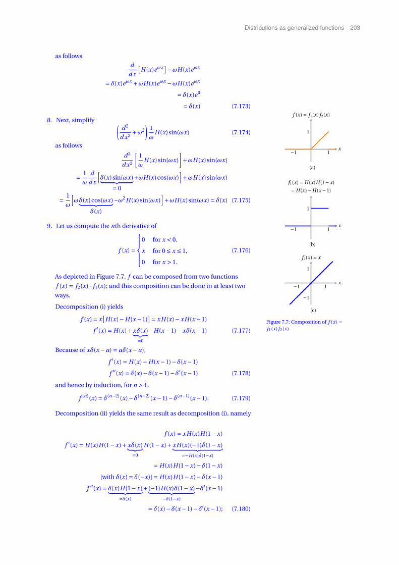
Distributions as generalized functions 203

as follows

d

d x

[H(x)eωx]−ωH(x)eωx

= δ(x)eωx +ωH(x)eωx −ωH(x)eωx

= δ(x)e0

= δ(x) (7.173)

8. Next, simplify (d 2

d x2 +ω2)

1

ωH(x)sin(ωx) (7.174)

as follows

d 2

d x2

[1

ωH(x)sin(ωx)

]+ωH(x)sin(ωx)

= 1

ω

d

d x

[δ(x)sin(ωx)︸ ︷︷ ︸

= 0

+ωH(x)cos(ωx)]+ωH(x)sin(ωx)

= 1

ω

[ωδ(x)cos(ωx)︸ ︷︷ ︸

δ(x)

−ω2H(x)sin(ωx)]+ωH(x)sin(ωx) = δ(x) (7.175)

−1 1

1

x

f (x) = f1(x) f2(x)

(a)

−1 1

1

x

f1(x) = H(x)H(1−x)

= H(x)−H(x −1)

(b)

−1 1

−1

1

x

f2(x) = x

(c)

Figure 7.7: Composition of f (x) =f1(x) f2(x).

9. Let us compute the nth derivative of

f (x) =

0 for x < 0,

x for 0 ≤ x ≤ 1,

0 for x > 1.

(7.176)

As depicted in Figure 7.7, f can be composed from two functions

f (x) = f2(x) · f1(x); and this composition can be done in at least two

ways.

Decomposition (i) yields

f (x) = x[H(x)−H(x −1)

]= xH(x)−xH(x −1)

f ′(x) = H(x)+xδ(x)︸ ︷︷ ︸=0

−H(x −1)−xδ(x −1) (7.177)

Because of xδ(x −a) = aδ(x −a),

f ′(x) = H(x)−H(x −1)−δ(x −1)

f ′′(x) = δ(x)−δ(x −1)−δ′(x −1) (7.178)

and hence by induction, for n > 1,

f (n)(x) = δ(n−2)(x)−δ(n−2)(x −1)−δ(n−1)(x −1). (7.179)

Decomposition (ii) yields the same result as decomposition (i), namely

f (x) = xH(x)H(1−x)

f ′(x) = H(x)H(1−x)+xδ(x)︸ ︷︷ ︸=0

H(1−x)+xH(x)(−1)δ(1−x)︸ ︷︷ ︸=−H(x)δ(1−x)

= H(x)H(1−x)−δ(1−x)

[with δ(x) = δ(−x)] = H(x)H(1−x)−δ(x −1)

f ′′(x) = δ(x)H(1−x)︸ ︷︷ ︸=δ(x)

+ (−1)H(x)δ(1−x)︸ ︷︷ ︸−δ(1−x)

−δ′(x −1)

= δ(x)−δ(x −1)−δ′(x −1); (7.180)

204 Mathematical Methods of Theoretical Physics

and hence by induction, for n > 1,

f (n)(x) = δ(n−2)(x)−δ(n−2)(x −1)−δ(n−1)(x −1). (7.181)

10. Let us compute the nth derivative of

f (x) =|sin x| for −π≤ x ≤π,

0 for |x| >π.(7.182)

f (x) = |sin x|H(π+x)H(π−x)

|sin x| = sin x sgn(sin x) = sin x sgn x for −π< x <π;

hence we start from

f (x) = sin x sgn xH(π+x)H(π−x),

Note that

sgn x = H(x)−H(−x),

( sgn x)′ = H ′(x)−H ′(−x)(−1) = δ(x)+δ(−x) = δ(x)+δ(x) = 2δ(x).

f ′(x) = cos x sgn xH(π+x)H(π−x)+ sin x2δ(x)H(π+x)H(π−x)++sin x sgn xδ(π+x)H(π−x)+ sin x sgn xH(π+x)δ(π−x)(−1) =

= cos x sgn xH(π+x)H(π−x)

f ′′(x) = −sin x sgn xH(π+x)H(π−x)+cos x2δ(x)H(π+x)H(π−x)++cos x sgn xδ(π+x)H(π−x)+cos x sgn xH(π+x)δ(π−x)(−1) =

= −sin x sgn xH(π+x)H(π−x)+2δ(x)+δ(π+x)+δ(π−x)

f ′′′(x) = −cos x sgn xH(π+x)H(π−x)− sin x2δ(x)H(π+x)H(π−x)−−sin x sgn xδ(π+x)H(π−x)− sin x sgn xH(π+x)δ(π−x)(−1)++2δ′(x)+δ′(π+x)−δ′(π−x) =

= −cos x sgn xH(π+x)H(π−x)+2δ′(x)+δ′(π+x)−δ′(π−x)

f (4)(x) = sin x sgn xH(π+x)H(π−x)−cos x2δ(x)H(π+x)H(π−x)−−cos x sgn xδ(π+x)H(π−x)−cos x sgn xH(π+x)δ(π−x)(−1)++2δ′′(x)+δ′′(π+x)+δ′′(π−x) =

= sin x sgn xH(π+x)H(π−x)−2δ(x)−δ(π+x)−δ(π−x)++2δ′′(x)+δ′′(π+x)+δ′′(π−x);

hence

f (4) = f (x)−2δ(x)+2δ′′(x)−δ(π+x)+δ′′(π+x)−δ(π−x)+δ′′(π−x),

f (5) = f ′(x)−2δ′(x)+2δ′′′(x)−δ′(π+x)+δ′′′(π+x)+δ′(π−x)−δ′′′(π−x);

and thus by induction

f (n) = f (n−4)(x)−2δ(n−4)(x)+2δ(n−2)(x)−δ(n−4)(π+x)++δ(n−2)(π+x)+ (−1)n−1δ(n−4)(π−x)+ (−1)nδ(n−2)(π−x)

(n = 4,5,6, . . . )

b

Part IIIDifferential equations

Green’s function 207

8Green’s function

This chapter is the beginning of a series of chapters dealing with the

solution of differential equations related to theoretical physics. These

differential equations are linear; that is, the “sought after” function

Ψ(x), y(x),φ(t) et cetera occur only as a polynomial of degree zero and

one, and not of any higher degree, such as, for instance, [y(x)]2.

8.1 Elegant way to solve linear differential equations

Green’s functions present a very elegant way of solving linear differential

equations of the form

Lx y(x) = f (x), with the differential operator

Lx = an(x)d n

d xn +an−1(x)d n−1

d xn−1 + . . .+a1(x)d

d x+a0(x)

=n∑

j=0a j (x)

d j

d x j, (8.1)

where ai (x), 0 ≤ i ≤ n are functions of x. The idea of the Green’s function

method is quite straightforward: if we are able to obtain the “inverse” G

of the differential operator L defined by

LxG(x, x ′) = δ(x −x ′), (8.2)

with δ representing Dirac’s delta function, then the solution to the inho-

mogeneous differential equation (8.1) can be obtained by integrating

G(x, x ′) alongside with the inhomogeneous term f (x ′); that is, by forming

y(x) =∫ ∞

−∞G(x, x ′) f (x ′)d x ′. (8.3)

208 Mathematical Methods of Theoretical Physics

This claim, as posted in Equation (8.3), can be verified by explicitly

applying the differential operator Lx to the solution y(x),

Lx y(x)

=Lx

∫ ∞

−∞G(x, x ′) f (x ′)d x ′

=∫ ∞

−∞LxG(x, x ′) f (x ′)d x ′

=∫ ∞

−∞δ(x −x ′) f (x ′)d x ′

= f (x). (8.4)

Let us check whether G(x, x ′) = H(x − x ′)sinh(x − x ′) is a Green’s

function of the differential operator Lx = d 2

d x2 −1. In this case, all we have

to do is to verify that Lx , applied to G(x, x ′), actually renders δ(x −x ′), as

required by Equation (8.2).

LxG(x, x ′) = δ(x −x ′)(d 2

d x2 −1

)H(x −x ′)sinh(x −x ′) ?= δ(x −x ′) (8.5)

Note that dd x sinh x = cosh x and d

d x cosh x = sinh x and, therefore,

d

d x

δ(x −x ′)sinh(x −x ′)︸ ︷︷ ︸= 0

+H(x −x ′)cosh(x −x ′)

−H(x −x ′)sinh(x −x ′)

= δ(x −x ′)cosh(x −x ′)︸ ︷︷ ︸=δ(x−x′)

+H(x −x ′)sinh(x −x ′)

−H(x −x ′)sinh(x −x ′) = δ(x −x ′). (8.6)

8.2 Nonuniqueness of solution

The solution (8.4) so obtained is not unique, as it is only a special solution

to the inhomogeneous equation (8.1). The general solution to (8.1) can

be found by adding the general solution y0(x) of the corresponding

homogeneous differential equation

Lx y0(x) = 0 (8.7)

to one special solution – say, the one obtained in Equation (8.4) through

Green’s function techniques.

Indeed, the most general solution

Y (x) = y(x)+ y0(x) (8.8)

clearly is a solution of the inhomogeneous differential equation (8.4), as

Lx Y (x) =Lx y(x)+Lx y0(x) = f (x)+0 = f (x). (8.9)

Conversely, any two distinct special solutions y1(x) and y2(x) of the in-

homogeneous differential equation (8.4) differ only by a function which

Green’s function 209

is a solution of the homogeneous differential equation (8.7), because due

to linearity of Lx , their difference y1(x)− y2(x) can be parameterized by

some function y0 which is the solution of the homogeneous differential

equation:

Lx [y1(x)− y2(x)] =Lx y1(x)+Lx y2(x) = f (x)− f (x) = 0. (8.10)

8.3 Green’s functions of translational invariant differential

operators

From now on, we assume that the coefficients a j (x) = a j in Equation

(8.1) are constants, and thus are translational invariant. Then the dif-

ferential operator Lx , as well as the entire Ansatz (8.2) for G(x, x ′), is

translation invariant, because derivatives are defined only by relative

distances, and δ(x −x ′) is translation invariant for the same reason. Hence,

G(x, x ′) =G(x −x ′). (8.11)

For such translation invariant systems, the Fourier analysis presents an

excellent way of analyzing the situation.

Let us see why translation invariance of the coefficients a j (x) =a j (x + ξ) = a j under the translation x → x + ξ with arbitrary ξ – that is,

independence of the coefficients a j on the “coordinate” or “parameter”

x – and thus of the Green’s function, implies a simple form of the latter.

Translanslation invariance of the Green’s function really means

G(x +ξ, x ′+ξ) =G(x, x ′). (8.12)

Now set ξ = −x ′; then we can define a new Green’s function that just

depends on one argument (instead of previously two), which is the

difference of the old arguments

G(x −x ′, x ′−x ′) =G(x −x ′,0) →G(x −x ′). (8.13)

8.4 Solutions with fixed boundary or initial values

For applications, it is important to adapt the solutions of some inhomo-

geneous differential equation to boundary and initial value problems. In

particular, a properly chosen G(x −x ′), in its dependence on the parameter

x, “inherits” some behavior of the solution y(x). Suppose, for instance,

we would like to find solutions with y(xi ) = 0 for some parameter values

xi , i = 1, . . . ,k. Then, the Green’s function G must vanish there also

G(xi −x ′) = 0 for i = 1, . . . ,k. (8.14)

8.5 Finding Green’s functions by spectral decompositions

It has been mentioned earlier (cf. Section 7.6.5 on page 188) that the

δ-function can be expressed in terms of various eigenfunction expansions.

We shall make use of these expansions here.1

1 Dean G. Duffy. Green’s Functions withApplications. Chapman and Hall/CRC,Boca Raton, 2001

210 Mathematical Methods of Theoretical Physics

Suppose ψi (x) are eigenfunctions of the differential operator Lx , and

λi are the associated eigenvalues; that is,

Lxψi (x) =λiψi (x). (8.15)

Suppose further that Lx is of degree n, and therefore (we assume with-

out proof) that we know all (a complete set of) the n eigenfunctions

ψ1(x),ψ2(x), . . . ,ψn(x) of Lx . In this case, orthogonality of the system of

eigenfunctions holds, such that∫ ∞

−∞ψi (x)ψ j (x)d x = δi j , (8.16)

as well as completeness, such that

n∑i=1

ψi (x ′)ψi (x) = δ(x −x ′). (8.17)

ψi (x ′) stands for the complex conjugate of ψi (x ′). The sum in Equation

(8.17) stands for an integral in the case of continuous spectrum of Lx .

In this case, the Kronecker δi j in (8.16) is replaced by the Dirac delta

function δ(k −k ′). It has been mentioned earlier that the δ-function can

be expressed in terms of various eigenfunction expansions.

The Green’s function of Lx can be written as the spectral sum of the

product of the (conjugate) eigenfunctions, divided by the eigenvalues λ j ;

that is,

G(x −x ′) =n∑

j=1

ψ j (x ′)ψ j (x)

λ j. (8.18)

For the sake of proof, apply the differential operator Lx to the Green’s

function Ansatz G of Equation (8.18) and verify that it satisfies Equation

(8.2):

LxG(x −x ′)

=Lx

n∑j=1

ψ j (x ′)ψ j (x)

λ j

=n∑

j=1

ψ j (x ′)[Lxψ j (x)]

λ j

=n∑

j=1

ψ j (x ′)[λ jψ j (x)]

λ j

=n∑

j=1ψ j (x ′)ψ j (x)

= δ(x −x ′). (8.19)

1. For a demonstration of completeness of systems of eigenfunctions,

consider, for instance, the differential equation corresponding to the

harmonic vibration [please do not confuse this with the harmonic

oscillator (6.29)]

Ltφ(t ) = d 2

d t 2φ(t ) = k2, (8.20)

with k ∈R.

Green’s function 211

Without any boundary conditions the associated eigenfunctions are

ψω(t ) = e±iωt , (8.21)

with 0 ≤ ω ≤∞, and with eigenvalue −ω2. Taking the complex con-

jugate ψω(t ′) of ψω(t ′) and integrating the product ψω(t)ψω(t ′) over

ω yields [modulo a constant factor which depends on the choice of

Fourier transform parameters; see also Equation (7.97)]∫ ∞

−∞ψω(t ′)ψω(t )dω

=∫ ∞

−∞e iωt ′e−iωt dω

=∫ ∞

−∞e−iω(t−t ′)dω

= 2πδ(t − t ′). (8.22)

The associated Green’s function – together with a prescription to

circumvent the pole at the origin – is defined by

G(t − t ′) =∫ ∞

−∞e±iω(t−t ′)

(−ω2)dω. (8.23)

The solution is obtained by multiplication with the constant k2, and

by integration over t ′; that is,

φ(t ) =∫ ∞

−∞G(t − t ′)k2d t ′ =−

∫ ∞

−∞

(k

ω

)2

e±iω(t−t ′)dω d t ′. (8.24)

Suppose that, additionally, we impose boundary conditions; e.g.,

φ(0) = φ(L) = 0, representing a string “fastened” at positions 0 and L.

In this case the eigenfunctions change to

ψn(t ) = sin(ωn t ) = sin(nπ

Lt)

, (8.25)

with ωn = nπL and n ∈Z. We can deduce orthogonality and complete-

ness from the orthogonality relations for sines (6.11).

2. For the sake of another example suppose, from the Euler-Bernoulli

bending theory, we know (no proof is given here) that the equation for

the quasistatic bending of slender, isotropic, homogeneous beams of

constant cross-section under an applied transverse load q(x) is given

by

Lx y(x) = d 4

d x4 y(x) = q(x) ≈ c, (8.26)

with constant c ∈R. Let us further assume the boundary conditions

y(0) = y(L) = d 2

d x2 y(0) = d 2

d x2 y(L) = 0. (8.27)

Also, we require that y(x) vanishes everywhere except inbetween 0 and

L; that is, y(x) = 0 for x = (−∞,0) and for x = (L,∞). Then in accor-

dance with these boundary conditions, the system of eigenfunctions

ψ j (x) of Lx can be written as

ψ j (x) =√

2

Lsin

(π j x

L

)(8.28)

212 Mathematical Methods of Theoretical Physics

for j = 1,2, . . .. The associated eigenvalues

λ j =(π j

L

)4

can be verified through explicit differentiation

Lxψ j (x) =Lx

√2

Lsin

(π j x

L

)=

(π j

L

)4√

2

Lsin

(π j x

L

)=

(π j

L

)4

ψ j (x). (8.29)

The cosine functions which are also solutions of the Euler-Bernoulli

equations (8.26) do not vanish at the origin x = 0.

Hence,

G(x −x ′) = 2

L

∞∑j=1

sin(π j x

L

)sin

(π j x′

L

)(π jL

)4

= 2L3

π4

∞∑j=1

1

j 4 sin

(π j x

L

)sin

(π j x ′

L

)(8.30)

Finally the solution can be calculated explicitly by

y(x) =∫ L

0G(x −x ′)g (x ′)d x ′

≈∫ L

0c

[2L3

π4

∞∑j=1

1

j 4 sin

(π j x

L

)sin

(π j x ′

L

)]d x ′

= 2cL3

π4

∞∑j=1

1

j 4 sin

(π j x

L

)[∫ L

0sin

(π j x ′

L

)d x ′

]

= 4cL4

π5

∞∑j=1

1

j 5 sin

(π j x

L

)sin2

(π j

2

)(8.31)

8.6 Finding Green’s functions by Fourier analysis

If one is dealing with translation invariant systems of the form

Lx y(x) = f (x), with the differential operator

Lx = and n

d xn +an−1d n−1

d xn−1 + . . .+a1d

d x+a0

=n∑

j=0a j

d j

d x j, (8.32)

with constant coefficients a j , then one can apply the following strategy

using Fourier analysis to obtain the Green’s function.

First, recall that, by Equation (7.96) on page 188 the Fourier transform

δ(k) of the delta function δ(x), as defined by the conventions A = B = 1 in

Equation (6.19), is just a constant 1. Therefore, δ can be written as A and B refer to Equation (6.19) onpage 167.

δ(x −x ′) = 1

2π

∫ ∞

−∞e i k(x−x′)dk (8.33)

Green’s function 213

Next, consider the Fourier transform of the Green’s function

G(k) =∫ ∞

−∞G(x)e−i kx d x (8.34)

and its inverse transform

G(x) = 1

2π

∫ ∞

−∞G(k)e i kx dk. (8.35)

Insertion of Equation (8.35) into the Ansatz LxG(x − x ′) = δ(x − x ′)yields

LxG(x) =Lx1

2π

∫ ∞

−∞G(k)e i kx dk = 1

2π

∫ ∞

−∞G(k)

(Lx e i kx

)dk

= δ(x) = 1

2π

∫ ∞

−∞e i kx dk. (8.36)

and thus, if Lx e i kx =P (k)e i kx , where P (k) is a polynomial in k,

1

2π

∫ ∞

−∞[G(k)P (k)−1

]e i kx dk = 0. (8.37)

Therefore, the bracketed part of the integral kernel needs to vanish; and Note that∫ ∞−∞ f (x)cos(kx)dk =

−i∫ ∞−∞ f (x)sin(kx)dk cannot be sat-

isfied for arbitrary x unless f (x) = 0.we obtain

G(k)P (k)−1 ≡ 0, or G(k) ≡ “(Lk )−1 ”, (8.38)

where Lk is obtained from Lx by substituting every derivative dd x in the

latter by i k in the former. As a result, the Fourier transform is obtained

through G(k) = 1/P (k); that is, as one divided by a polynomial P (k) of

degree n, the same degree as the highest order of derivative in Lx .

In order to obtain the Green’s function G(x), and to be able to integrate

over it with the inhomogeneous term f (x), we have to Fourier transform

G(k) back to G(x).

Note that if one solves the Fourier integration by analytic continuation

into the k-plane, different integration paths lead to special solutions

which are different only by some particular solution of the homogeneous

differential equation.

Then we have to make sure that the solution obeys the initial condi-

tions, and, if necessary, we have to add solutions of the homogeneous

equation LxG(x −x ′) = 0. That is all.

Let us consider a few examples for this procedure.

1. First, let us solve the differential equation y ′− y = t on the interval

[0,∞) with the boundary conditions y(0) = 0.

We observe that the associated differential operator is given by

Lt = d

d t−1,

and the inhomogeneous term can be identified with f (t ) = t .

We use the Ansatz G1(t , t ′) = 12π

+∞∫−∞

G1(k)e i k(t−t ′)dk; hence

Lt G1(t , t ′) = 1

2π

+∞∫−∞

G1(k)

(d

d t−1

)e i k(t−t ′)︸ ︷︷ ︸

= (i k −1)e i k(t−t ′)

dk

= δ(t − t ′) = 1

2π

+∞∫−∞

e i k(t−t ′)dk (8.39)

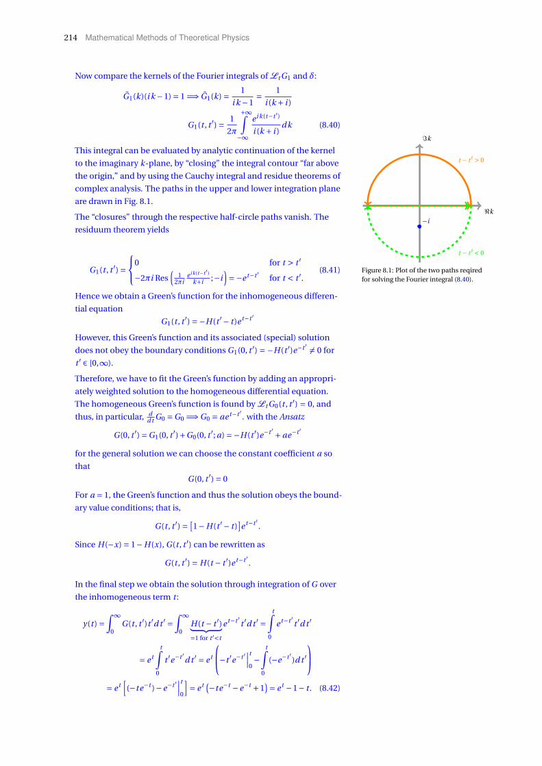
214 Mathematical Methods of Theoretical Physics

Now compare the kernels of the Fourier integrals of Lt G1 and δ:

G1(k)(i k −1) = 1 =⇒ G1(k) = 1

i k −1= 1

i (k + i )

G1(t , t ′) = 1

2π

+∞∫−∞

e i k(t−t ′)

i (k + i )dk (8.40)

This integral can be evaluated by analytic continuation of the kernel

to the imaginary k-plane, by “closing” the integral contour “far above

the origin,” and by using the Cauchy integral and residue theorems of

complex analysis. The paths in the upper and lower integration plane

are drawn in Fig. 8.1.

ℑk

ℜk

t − t ′ > 0

t − t ′ < 0

−i

Figure 8.1: Plot of the two paths reqiredfor solving the Fourier integral (8.40).

The “closures” through the respective half-circle paths vanish. The

residuum theorem yields

G1(t , t ′) =0 for t > t ′

−2πi Res(

12πi

ei k(t−t ′)k+i ;−i

)=−e t−t ′ for t < t ′.

(8.41)

Hence we obtain a Green’s function for the inhomogeneous differen-

tial equation

G1(t , t ′) =−H(t ′− t )e t−t ′

However, this Green’s function and its associated (special) solution

does not obey the boundary conditions G1(0, t ′) = −H(t ′)e−t ′ 6= 0 for

t ′ ∈ [0,∞).

Therefore, we have to fit the Green’s function by adding an appropri-

ately weighted solution to the homogeneous differential equation.

The homogeneous Green’s function is found by Lt G0(t , t ′) = 0, and

thus, in particular, dd t G0 =G0 =⇒G0 = ae t−t ′ . with the Ansatz

G(0, t ′) =G1(0, t ′)+G0(0, t ′; a) =−H(t ′)e−t ′ +ae−t ′

for the general solution we can choose the constant coefficient a so

that

G(0, t ′) = 0

For a = 1, the Green’s function and thus the solution obeys the bound-

ary value conditions; that is,

G(t , t ′) = [1−H(t ′− t )

]e t−t ′ .

Since H(−x) = 1−H(x), G(t , t ′) can be rewritten as

G(t , t ′) = H(t − t ′)e t−t ′ .

In the final step we obtain the solution through integration of G over

the inhomogeneous term t :

y(t ) =∫ ∞

0G(t , t ′)t ′d t ′ =

∫ ∞

0H(t − t ′)︸ ︷︷ ︸=1 for t ′<t

e t−t ′ t ′d t ′ =t∫

0

e t−t ′ t ′d t ′

= e t

t∫0

t ′e−t ′d t ′ = e t

−t ′e−t ′∣∣∣t

0−

t∫0

(−e−t ′ )d t ′

= e t[

(−te−t )−e−t ′∣∣∣t

0

]= e t (−te−t −e−t +1

)= e t −1− t . (8.42)

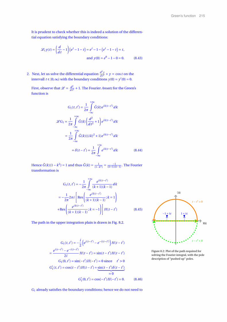
Green’s function 215

It is prudent to check whether this is indeed a solution of the differen-

tial equation satisfying the boundary conditions:

Lt y(t ) =(

d

d t−1

)(e t −1− t

)= e t −1− (e t −1− t

)= t ,

and y(0) = e0 −1−0 = 0. (8.43)

2. Next, let us solve the differential equation d 2 yd t 2 + y = cos t on the

intervall t ∈ [0,∞) with the boundary conditions y(0) = y ′(0) = 0.

First, observe that L = d 2

d t 2 + 1. The Fourier Ansatz for the Green’s

function is

G1(t , t ′) = 1

2π

+∞∫−∞

G(k)e i k(t−t ′)dk

L G1 = 1

2π

+∞∫−∞

G(k)

(d 2

d t 2 +1

)e i k(t−t ′)dk

= 1

2π

+∞∫−∞

G(k)((i k)2 +1)e i k(t−t ′)dk

= δ(t − t ′) = 1

2π

+∞∫−∞

e i k(t−t ′)dk (8.44)

Hence G(k)(1−k2) = 1 and thus G(k) = 1(1−k2)

= −1(k+1)(k−1) . The Fourier

transformation is

G1(t , t ′) =− 1

2π

+∞∫−∞

e i k(t−t ′)

(k +1)(k −1)dk

=− 1

2π2πi

[Res

(e i k(t−t ′)

(k +1)(k −1);k = 1

)

+Res

(e i k(t−t ′)

(k +1)(k −1);k =−1

)]H(t − t ′) (8.45)

The path in the upper integration plain is drawn in Fig. 8.2.

ℑk

ℜk

t − t ′ > 0

t − t ′ < 0

−1+ iε 1+ iε

Figure 8.2: Plot of the path required forsolving the Fourier integral, with the poledescription of “pushed up“ poles.

G1(t , t ′) =− i

2

(e i (t−t ′) −e−i (t−t ′)

)H(t − t ′)

= e i (t−t ′) −e−i (t−t ′)

2iH(t − t ′) = sin(t − t ′)H(t − t ′)

G1(0, t ′) = sin(−t ′)H(−t ′) = 0 since t ′ > 0

G ′1(t , t ′) = cos(t − t ′)H(t − t ′)+ sin(t − t ′)δ(t − t ′)︸ ︷︷ ︸

= 0

G ′1(0, t ′) = cos(−t ′)H(−t ′) = 0. (8.46)

G1 already satisfies the boundary conditions; hence we do not need to

216 Mathematical Methods of Theoretical Physics

find the Green’s function G0 of the homogeneous equation.

y(t ) =∞∫

0

G(t , t ′) f (t ′)d t ′ =∞∫

0

sin(t − t ′) H(t − t ′)︸ ︷︷ ︸= 1 for t > t ′

cos t ′d t ′

=t∫

0

sin(t − t ′)cos t ′d t ′ =t∫

0

(sin t cos t ′−cos t sin t ′)cos t ′d t ′

=t∫

0

[sin t (cos t ′)2 −cos t sin t ′ cos t ′

]d t ′ =

= sin t

t∫0

(cos t ′)2d t ′−cos t

t∫0

si nt ′ cos t ′d t ′

= sin t

[1

2(t ′+ sin t ′ cos t ′)

]∣∣∣∣t

0−cos t

[sin2 t ′

2

]∣∣∣∣t

0

= t sin t

2+ sin2 t cos t

2− cos t sin2 t

2= t sin t

2. (8.47)

\

Sturm-Liouville theory 217

9Sturm-Liouville theory

This is only a very brief “dive into Sturm-Liouville theory,” which has

many fascinating aspects and connections to Fourier analysis, the special

functions of mathematical physics, operator theory, and linear algebra.1 1 Garrett Birkhoff and Gian-Carlo Rota.Ordinary Differential Equations. JohnWiley & Sons, New York, Chichester,Brisbane, Toronto, fourth edition, 1959,1960, 1962, 1969, 1978, and 1989; M. A.Al-Gwaiz. Sturm-Liouville Theory andits Applications. Springer, London, 2008;and William Norrie Everitt. A catalogueof Sturm-Liouville differential equations.In Werner O. Amrein, Andreas M. Hinz,and David B. Pearson, editors, Sturm-Liouville Theory, Past and Present, pages271–331. Birkhäuser Verlag, Basel, 2005.URL http://www.math.niu.edu/SL2/

papers/birk0.pdf

In physics, many formalizations involve second order linear ordinary

differential equations (ODEs), which, in their most general form, can be

Here the term ordinary – in contrastwith partial – is used to indicate thatits termms and solutions just dependon a single one independent variable.Typical examples of a partial differentialequations are the Laplace or the waveequation in three spatial dimensions.

written as2

2 Russell Herman. A Second Coursein Ordinary Differential Equations:Dynamical Systems and BoundaryValue Problems. University of NorthCarolina Wilmington, Wilmington,NC, 2008. URL http://people.uncw.

edu/hermanr/pde1/PDEbook/index.

htm. Creative Commons Attribution-NoncommercialShare Alike 3.0 UnitedStates License

Lx y(x) = a0(x)y(x)+a1(x)d

d xy(x)+a2(x)

d 2

d x2 y(x) = f (x). (9.1)

The differential operator associated with this differential equation is

defined by

Lx = a0(x)+a1(x)d

d x+a2(x)

d 2

d x2 . (9.2)

The solutions y(x) are often subject to boundary conditions of various

forms:

• Dirichlet boundary conditions are of the form y(a) = y(b) = 0 for some

a,b.

• (Carl Gottfried) Neumann boundary conditions are of the form y ′(a) =y ′(b) = 0 for some a,b.

• Periodic boundary conditions are of the form y(a) = y(b) and y ′(a) =y ′(b) for some a,b.

9.1 Sturm-Liouville form

Any second order differential equation of the general form (9.1) can be

rewritten into a differential equation of the Sturm-Liouville form

Sx y(x) = d

d x

[p(x)

d

d x

]y(x)+q(x)y(x) = F (x),

with p(x) = e∫ a1(x)

a2(x) d x,

q(x) = p(x)a0(x)

a2(x)= a0(x)

a2(x)e

∫ a1(x)a2(x) d x

,

F (x) = p(x)f (x)

a2(x)= f (x)

a2(x)e

∫ a1(x)a2(x) d x

(9.3)

218 Mathematical Methods of Theoretical Physics

The associated differential operator

Sx = d

d x

[p(x)

d

d x

]+q(x)

= p(x)d 2

d x2 +p ′(x)d

d x+q(x) (9.4)

is called Sturm-Liouville differential operator. It is very special: compared

to the general form (9.1) the transformation (9.3) yields

a1(x) = a′2(x). (9.5)

For a proof, we insert p(x), q(x) and F (x) into the Sturm-Liouville

form of Equation (9.3) and compare it with Equation (9.1).

d

d x

[e

∫ a1(x)a2(x) d x d

d x

]+ a0(x)

a2(x)e

∫ a1(x)a2(x) d x

y(x) = f (x)

a2(x)e

∫ a1(x)a2(x) d x

e∫ a1(x)

a2(x) d x

d 2

d x2 + a1(x)

a2(x)

d

d x+ a0(x)

a2(x)

y(x) = f (x)

a2(x)e

∫ a1(x)a2(x) d x

a2(x)

d 2

d x2 +a1(x)d

d x+a0(x)

y(x) = f (x). (9.6)

9.2 Adjoint and self-adjoint operators

In operator theory, just as in matrix theory, we can define an adjoint op-

erator (for finite dimensional Hilbert space, see Section 1.18 on page 43)

via the scalar product defined in Equation (9.25). In this formalization,

the Sturm-Liouville differential operator S is self-adjoint.

Let us first define the domain of a differential operator L as the set

of all square integrable (with respect to the weight ρ(x)) functions ϕ

satisfying boundary conditions.∫ b

a|ϕ(x)|2ρ(x)d x <∞. (9.7)

Then, the adjoint operator L † is defined by satisfying

⟨ψ |Lϕ⟩ =∫ b

aψ(x)[Lϕ(x)]ρ(x)d x

= ⟨L †ψ |ϕ⟩ =∫ b

a[L †ψ(x)]ϕ(x)ρ(x)d x (9.8)

for all ψ(x) in the domain of L † and ϕ(x) in the domain of L .

Note that in the case of second order differential operators in the

standard form (9.2) and with ρ(x) = 1, we can move the differential

quotients and the entire differential operator in

⟨ψ |Lϕ⟩ =∫ b

aψ(x)[Lxϕ(x)]ρ(x)d x

=∫ b

aψ(x)[a2(x)ϕ′′(x)+a1(x)ϕ′(x)+a0(x)ϕ(x)]d x (9.9)

from ϕ to ψ by one and two partial integrations.

Sturm-Liouville theory 219

Integrating the kernel a1(x)ϕ′(x) by parts yields∫ b

aψ(x)a1(x)ϕ′(x)d x = ψ(x)a1(x)ϕ(x)

∣∣ba −

∫ b

a(ψ(x)a1(x))′ϕ(x)d x. (9.10)

Integrating the kernel a2(x)ϕ′′(x) by parts twice yields∫ b

aψ(x)a2(x)ϕ′′(x)d x = ψ(x)a2(x)ϕ′(x)

∣∣ba −

∫ b

a(ψ(x)a2(x))′ϕ′(x)d x

= ψ(x)a2(x)ϕ′(x)∣∣b

a − (ψ(x)a2(x))′ϕ(x)∣∣b

a +∫ b

a(ψ(x)a2(x))′′ϕ(x)d x

= ψ(x)a2(x)ϕ′(x)− (ψ(x)a2(x))′ϕ(x)∣∣b

a +∫ b

a(ψ(x)a2(x))′′ϕ(x)d x.

(9.11)

Combining these two calculations yields

⟨ψ |Lϕ⟩ =∫ b

aψ(x)[Lxϕ(x)]ρ(x)d x

=∫ b

aψ(x)[a2(x)ϕ′′(x)+a1(x)ϕ′(x)+a0(x)ϕ(x)]d x

= ψ(x)a1(x)ϕ(x)+ψ(x)a2(x)ϕ′(x)− (ψ(x)a2(x))′ϕ(x)∣∣b

a

+∫ b

a[(a2(x)ψ(x))′′− (a1(x)ψ(x))′+a0(x)ψ(x)]ϕ(x)d x. (9.12)

If the boundary terms vanish because of boundary conditions on ψ,

ϕ, ψ′, ϕ′ or for other reasons, such as a1(x) = a′2(x) in the case of the

Sturm-Liouville operator Sx ; that is, if

ψ(x)a1(x)ϕ(x)+ψ(x)a2(x)ϕ′(x)− (ψ(x)a2(x))′ϕ(x)∣∣b

a = 0, (9.13)

then Equation (9.12) reduces to

⟨ψ |Lϕ⟩ =∫ b

a[(a2(x)ψ(x))′′− (a1(x)ψ(x))′+a0(x)ψ(x)]ϕ(x)d x, (9.14)

and we can identify the adjoint differential operator of Lx with

L †x = d 2

d x2 a2(x)− d

d xa1(x)+a0(x)

= d

d x

[a2(x)

d

d x+a′

2(x)

]−a′

1(x)−a1(x)d

d x+a0(x)

= a′2(x)

d

d x+a2(x)

d 2

d x2 +a′′2 (x)+a′

2(x)d

d x−a′

1(x)−a1(x)d

d x+a0(x)

= a2(x)︸ ︷︷ ︸a2

d 2

d x2 + [2a′2(x)−a1(x)]︸ ︷︷ ︸

a1

d

d x+a′′

2 (x)−a′1(x)+a0(x)︸ ︷︷ ︸a0

.

(9.15)

The operator Lx is called self-adjoint if

L †x =Lx ; (9.16)

that is, if a1 = a1, a2 = a2, and a3 = a3.

Next we shall show that, in particular, the Sturm-Liouville differential

operator (9.4) is self-adjoint, and that all second order differential opera-

tors [with the boundary condition (9.13)] which are self-adjoint are of the

Sturm-Liouville form.

220 Mathematical Methods of Theoretical Physics

In order to prove that the Sturm-Liouville differential operator

S = d

d x

[p(x)

d

d x

]+q(x) = p(x)

d 2

d x2 +p ′(x)d

d x+q(x) (9.17)

from Equation (9.4) is self-adjoint, we verify Equation (9.16) with S †

taken from Equation (9.15). Thereby, we identify a2(x) = p(x), a1(x) =p ′(x), and a0(x) = q(x); hence

S †x = a2(x)

d 2

d x2 + [2a′2(x)−a1(x)]

d

d x+a′′

2 (x)−a′1(x)+a0(x)

= p(x)d 2

d x2 + [2p ′(x)−p ′(x)]d

d x+p ′′(x)−p ′′(x)+q(x)

= p(x)d 2

d x2 +p ′(x)d

d x+q(x) =Sx . (9.18)

Alternatively we could argue from Eqs. (9.15) and (9.16), noting that a

differential operator is self-adjoint if and only if

Lx = a2(x)d 2

d x2 +a1(x)d

d x+a0(x)

=L †x = a2(x)

d 2

d x2 + [2a′2(x)−a1(x)]

d

d x+a′′

2 (x)−a′1(x)+a0(x). (9.19)

By comparison of the coefficients,

a2(x) = a2(x),

a1(x) = 2a′2(x)−a1(x),

a0(x) = a′′2 (x)−a′

1(x)+a0(x), (9.20)

and hence,

a′2(x) = a1(x), (9.21)

which is exactly the form of the Sturm-Liouville differential operator.

9.3 Sturm-Liouville eigenvalue problem

The Sturm-Liouville eigenvalue problem is given by the differential

equation The minus sign “−λ” is here for purelyconvential reasons; to make the presenta-tion compatible with other texts.Sxφ(x) =−λρ(x)φ(x), or

d

d x

[p(x)

d

d x

]φ(x)+ [q(x)+λρ(x)]φ(x) = 0 (9.22)

for x ∈ (a,b) and continuous p ′(x), q(x) and p(x) > 0, ρ(x) > 0.

It can be expected that, very similar to the spectral theory of linear

algebra introduced in Section 1.27.1 on page 63, self-adjoint operators

have a spectral decomposition involving real, ordered eigenvalues and

complete sets of mutually orthogonal operators. We mention without

proof (for proofs, see, for instance, Ref.3) that we can formulate a spectral 3 M. A. Al-Gwaiz. Sturm-Liouville Theoryand its Applications. Springer, London,2008

theorem as follows

• the eigenvalues λ turn out to be real, countable, and ordered, and that

there is a smallest eigenvalue λ1 such that λ1 <λ2 <λ3 < ·· · ;

Sturm-Liouville theory 221

• for each eigenvalue λ j there exists an eigenfunction φ j (x) with j −1

zeroes on (a,b);

• eigenfunctions corresponding to different eigenvalues are orthogonal,

and can be normalized, with respect to the weight function ρ(x); that

is,

⟨φ j |φk⟩ =∫ b

aφ j (x)φk (x)ρ(x)d x = δ j k (9.23)

• the set of eigenfunctions is complete; that is, any piecewise smooth

function can be represented by

f (x) =∞∑

k=1ckφk (x),

with

ck = ⟨ f |φk⟩⟨φk |φk⟩

= ⟨ f |φk⟩. (9.24)

• the orthonormal (with respect to the weight ρ) set φ j (x) | j ∈N is a

basis of a Hilbert space with the inner product

⟨ f | g ⟩ =∫ b

af (x)g (x)ρ(x)d x. (9.25)

9.4 Sturm-Liouville transformation into Liouville normal

form

Let, for x ∈ [a,b],

[Sx +λρ(x)]y(x) = 0,

d

d x

[p(x)

d

d x

]y(x)+ [q(x)+λρ(x)]y(x) = 0,[

p(x)d 2

d x2 +p ′(x)d

d x+q(x)+λρ(x)

]y(x) = 0,[

d 2

d x2 + p ′(x)

p(x)

d

d x+ q(x)+λρ(x)

p(x)

]y(x) = 0 (9.26)

be a second order differential equation of the Sturm-Liouville form.4 4 Garrett Birkhoff and Gian-Carlo Rota.Ordinary Differential Equations. JohnWiley & Sons, New York, Chichester,Brisbane, Toronto, fourth edition, 1959,1960, 1962, 1969, 1978, and 1989

This equation (9.26) can be written in the Liouville normal form

containing no first order differentiation term

− d 2

d t 2 w(t )+ [q(t )−λ]w(t ) = 0, with t ∈ [t (a), t (b)]. (9.27)

It is obtained via the Sturm-Liouville transformation

ξ= t (x) =∫ x

a

√ρ(s)

p(s)d s,

w(t ) = 4√

p(x(t ))ρ(x(t ))y(x(t )), (9.28)

where

q(t ) = 1

ρ

[−q − 4

ppρ

(p

(1

4p

pρ

)′)′]. (9.29)

The apostrophe represents derivation with respect to x.

222 Mathematical Methods of Theoretical Physics

For the sake of an example, suppose we want to know the normalized

eigenfunctions of

x2 y ′′+3x y ′+ y =−λy , with x ∈ [1,2] (9.30)

with the boundary conditions y(1) = y(2) = 0.

The first thing we have to do is to transform this differential equation

into its Sturm-Liouville form by identifying a2(x) = x2, a1(x) = 3x, a0 = 1,

ρ = 1 such that f (x) =−λy(x); and hence

p(x) = e∫ 3x

x2 d x = e∫ 3

x d x = e3log x = x3,

q(x) = p(x)1

x2 = x,

F (x) = p(x)λy

(−x2)=−λx y , and hence ρ(x) = x. (9.31)

As a result we obtain the Sturm-Liouville form

1

x((x3 y ′)′+x y) =−λy . (9.32)

In the next step we apply the Sturm-Liouville transformation

ξ= t (x) =∫ √

ρ(x)

p(x)d x =

∫d x

x= log x,

w(t (x)) = 4√

p(x(t ))ρ(x(t ))y(x(t )) = 4√

x4 y(x(t )) = x y ,

q(t ) = 1

x

[−x − 4

√x4

(x3

(1

4px4

)′)′]= 0. (9.33)

We now take the Ansatz y = 1x w(t(x)) = 1

x w(log x) and finally obtain the

Liouville normal form

−w ′′(ξ) =λw(ξ). (9.34)

As an Ansatz for solving the Liouville normal form we use

w(ξ) = a sin(pλξ)+b cos(

pλξ) (9.35)

The boundary conditions translate into x = 1 → ξ= 0, and x = 2 → ξ=log2. From w(0) = 0 we obtain b = 0. From w(log2) = a sin(

pλ log2) = 0

we obtain√λn log2 = nπ.

Thus the eigenvalues are

λn =(

nπ

log2

)2

. (9.36)

The associated eigenfunctions are

wn(ξ) = a sin

(nπ

log2ξ

), (9.37)

and thus

yn = 1

xa sin

(nπ

log2log x

). (9.38)

We can check that they are orthonormal by inserting into Equation

(9.23) and verifying it; that is,

2∫1

ρ(x)yn(x)ym(x)d x = δnm ; (9.39)

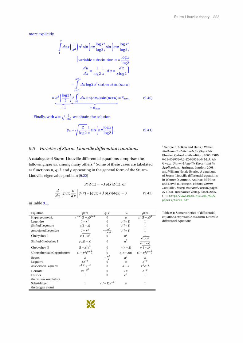
Sturm-Liouville theory 223

more explicitly,

2∫1

d xx

(1

x2

)a2 sin

(nπ

log x

log2

)sin

(mπ

log x

log2

)

[variable substitution u = log x

log2

du

d x= 1

log2

1

x, du = d x

x log2]

=u=1∫

u=0

du log2a2 sin(nπu)sin(mπu)

= a2(

log2

2

)︸ ︷︷ ︸

= 1

2∫ 1

0du sin(nπu)sin(mπu)︸ ︷︷ ︸

= δnm

= δnm . (9.40)

Finally, with a =√

2log2 we obtain the solution

yn =√

2

log2

1

xsin

(nπ

log x

log2

). (9.41)

9.5 Varieties of Sturm-Liouville differential equations

A catalogue of Sturm-Liouville differential equations comprises the

following species, among many others.5 Some of these cases are tabelated

5 George B. Arfken and Hans J. Weber.Mathematical Methods for Physicists.Elsevier, Oxford, sixth edition, 2005. ISBN0-12-059876-0;0-12-088584-0; M. A. Al-Gwaiz. Sturm-Liouville Theory and itsApplications. Springer, London, 2008;and William Norrie Everitt. A catalogueof Sturm-Liouville differential equations.In Werner O. Amrein, Andreas M. Hinz,and David B. Pearson, editors, Sturm-Liouville Theory, Past and Present, pages271–331. Birkhäuser Verlag, Basel, 2005.URL http://www.math.niu.edu/SL2/

papers/birk0.pdf

as functions p, q , λ and ρ appearing in the general form of the Sturm-

Liouville eigenvalue problem (9.22)

Sxφ(x) =−λρ(x)φ(x), or

d

d x

[p(x)

d

d x

]φ(x)+ [q(x)+λρ(x)]φ(x) = 0 (9.42)

in Table 9.1.

Equation p(x) q(x) −λ ρ(x)

Hypergeometric xα+1(1−x)β+1 0 µ xα(1−x)β

Legendre 1−x2 0 l (l +1) 1Shifted Legendre x(1−x) 0 l (l +1) 1

Associated Legendre 1−x2 − m2

1−x2 l (l +1) 1

Chebyshev I√

1−x2 0 n2 1p1−x2

Shifted Chebyshev Ip

x(1−x) 0 n2 1px(1−x)

Chebyshev II (1−x2)32 0 n(n +2)

√1−x2

Ultraspherical (Gegenbauer) (1−x2)α+12 0 n(n +2α) (1−x2)α−

12

Bessel x − n2

x a2 xLaguerre xe−x 0 α e−x

Associated Laguerre xk+1e−x 0 α−k xk e−x

Hermite xe−x20 2α e−x

Fourier 1 0 k2 1(harmonic oscillator)Schrödinger 1 l (l +1)x−2 µ 1(hydrogen atom)

Table 9.1: Some varieties of differentialequations expressible as Sturm-Liouvilledifferential equations

X

Separation of variables 225

10Separation of variables

This chapter deals with the ancient alchemic suspicion of “solve et co-

agula” that it is possible to solve a problem by splitting it up into partial

problems, solving these issues separately; and consecutively joining

together the partial solutions, thereby yielding the full answer to the

problem – translated into the context of partial differential equations; For a counterexample see the Kochen-Specker theorem on page 78.that is, equations with derivatives of more than one variable. Thereby,

solving the separate partial problems is not dissimilar to applying subpro-

grams from some program library.

Already Descartes mentioned this sort of method in his Discours

de la méthode pour bien conduire sa raison et chercher la verité dans

les sciences (English translation: Discourse on the Method of Rightly

Conducting One’s Reason and of Seeking Truth)1 stating that (in a newer 1 Rene Descartes. Discours de la méthodepour bien conduire sa raison et chercherla verité dans les sciences (Discourse onthe Method of Rightly Conducting One’sReason and of Seeking Truth). 1637. URLhttp://www.gutenberg.org/etext/59

translation2)

2 Rene Descartes. The PhilosophicalWritings of Descartes. Volume 1. Cam-bridge University Press, Cambridge, 1985.translated by John Cottingham, RobertStoothoff and Dugald Murdoch

[Rule Five:] The whole method consists entirely in the ordering and ar-

ranging of the objects on which we must concentrate our mind’s eye if we

are to discover some truth. We shall be following this method exactly if we

first reduce complicated and obscure propositions step by step to simpler

ones, and then, starting with the intuition of the simplest ones of all, try

to ascend through the same steps to a knowledge of all the rest. . . . [Rule

Thirteen:] If we perfectly understand a problem we must abstract it from

every superfluous conception, reduce it to its simplest terms and, by means

of an enumeration, divide it up into the smallest possible parts.

The method of separation of variables is one among a couple of

strategies to solve differential equations,3 and it is a very important one

3 Lawrence C. Evans. Partial differentialequations, volume 19 of Graduate Studiesin Mathematics. American Mathemat-ical Society, Providence, Rhode Island,1998; and Klaus Jänich. Analysis fürPhysiker und Ingenieure. Funktionenthe-orie, Differentialgleichungen, SpezielleFunktionen. Springer, Berlin, Heidel-berg, fourth edition, 2001. URL http:

//www.springer.com/mathematics/

analysis/book/978-3-540-41985-3

in physics.

Separation of variables can be applied whenever we have no “mixtures

of derivatives and functional dependencies;” more specifically, whenever

the partial differential equation can be written as a sum

Lx,yψ(x, y) = (Lx +Ly )ψ(x, y) = 0, or

Lxψ(x, y) =−Lyψ(x, y).(10.1)

Because in this case we may make a multiplicative4 Ansatz

4 Another possibility is an additivecomposition of the solution; cf. YonahCherniavsky. A note on separationof variables. International Journal ofMathematical Education in Science andTechnology, 42(1):129–131, 2011. D O I :10.1080/0020739X.2010.519793. URLhttps://doi.org/10.1080/0020739X.

2010.519793.ψ(x, y) = v(x)u(y). (10.2)

226 Mathematical Methods of Theoretical Physics

Inserting (10.2) into (10) effectively separates the variable dependencies

Lx v(x)u(y) =−Ly v(x)u(y),

u(y) [Lx v(x)] =−v(x)[Ly u(y)

],

1v(x) Lx v(x) =− 1

u(y) Ly u(y) = a,

(10.3)

with constant a, because Lx v(x)v(x) does not depend on x, and

Ly u(y)u(y) does

not depend on y . Therefore, neither side depends on x or y ; hence both

sides are constants.

As a result, we can treat and integrate both sides separately; that is,

1v(x) Lx v(x) = a,

1u(y) Ly u(y) =−a,

(10.4)

orLx v(x)−av(x) = 0,

Ly u(y)+au(y) = 0.(10.5)

This separation of variable Ansatz can be often used when the Laplace

operator ∆ = ∇ ·∇ is involved, since there the partial derivatives with

respect to different variables occur in different summands.

The general solution is a linear combination (superposition) of the If we would just consider a single productof all general one parameter solutions wewould run into the same problem as inthe entangled case on page 27 – we couldnot cover all the solutions of the originalequation.

products of all the linear independent solutions – that is, the sum of the

products of all separate (linear independent) solutions, weighted by an

arbitrary scalar factor.

For the sake of demonstration, let us consider a few examples.

1. Let us separate the homogeneous Laplace differential equation

∆Φ= 1

u2 + v2

(∂2Φ

∂u2 + ∂2Φ

∂v2

)+ ∂2Φ

∂z2 = 0 (10.6)

in parabolic cylinder coordinates (u, v , z) with x = ( 12 (u2 − v2),uv , z

).

The separation of variables Ansatz is

Φ(u, v , z) =Φ1(u)Φ2(v)Φ3(z). (10.7)

Inserting (10.7) into (10.6) yields

1

u2 + v2

(Φ2Φ3

∂2Φ1

∂u2 +Φ1Φ3∂2Φ2

∂v2

)+Φ1Φ2

∂2Φ3

∂z2 = 0

1

u2 + v2

(Φ′′

1

Φ1+ Φ

′′2

Φ2

)=−Φ

′′3

Φ3=λ= const.

λ is constant because it does neither depend on u, v [because of the

right hand sideΦ′′3 (z)/Φ3(z)], nor on z (because of the left hand side).

Furthermore,

Φ′′1

Φ1−λu2 =−Φ

′′2

Φ2+λv2 = l 2 = const.

with constant l for analogous reasons. The three resulting differential

equations are

Φ′′1 − (λu2 + l 2)Φ1 = 0,

Φ′′2 − (λv2 − l 2)Φ2 = 0,

Φ′′3 +λΦ3 = 0.

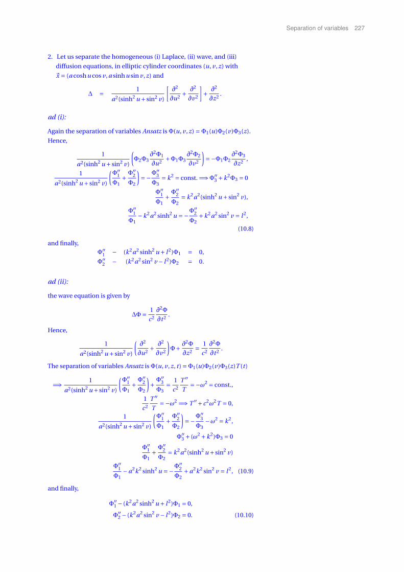
Separation of variables 227

2. Let us separate the homogeneous (i) Laplace, (ii) wave, and (iii)

diffusion equations, in elliptic cylinder coordinates (u, v , z) with

~x = (a coshu cos v , a sinhu sin v , z) and

∆ = 1

a2(sinh2 u + sin2 v)

[∂2

∂u2 + ∂2

∂v2

]+ ∂2

∂z2 .

ad (i):

Again the separation of variables Ansatz isΦ(u, v , z) =Φ1(u)Φ2(v)Φ3(z).

Hence,

1

a2(sinh2 u + sin2 v)

(Φ2Φ3

∂2Φ1

∂u2 +Φ1Φ3∂2Φ2

∂v2

)=−Φ1Φ2

∂2Φ3

∂z2 ,

1

a2(sinh2 u + sin2 v)

(Φ′′

1

Φ1+ Φ

′′2

Φ2

)=−Φ

′′3

Φ3= k2 = const. =⇒Φ′′

3 +k2Φ3 = 0

Φ′′1

Φ1+ Φ

′′2

Φ2= k2a2(sinh2 u + sin2 v),

Φ′′1

Φ1−k2a2 sinh2 u =−Φ

′′2

Φ2+k2a2 sin2 v = l 2,

(10.8)

and finally,Φ′′

1 − (k2a2 sinh2 u + l 2)Φ1 = 0,

Φ′′2 − (k2a2 sin2 v − l 2)Φ2 = 0.

ad (ii):

the wave equation is given by

∆Φ= 1

c2

∂2Φ

∂t 2 .

Hence,

1

a2(sinh2 u + sin2 v)

(∂2

∂u2 + ∂2

∂v2

)Φ+ ∂2Φ

∂z2 = 1

c2

∂2Φ

∂t 2 .

The separation of variables Ansatz isΦ(u, v , z, t ) =Φ1(u)Φ2(v)Φ3(z)T (t )

=⇒ 1

a2(sinh2 u + sin2 v)

(Φ′′

1

Φ1+ Φ

′′2

Φ2

)+ Φ

′′3

Φ3= 1

c2

T ′′

T=−ω2 = const.,

1

c2

T ′′

T=−ω2 =⇒ T ′′+ c2ω2T = 0,

1

a2(sinh2 u + sin2 v)

(Φ′′

1

Φ1+ Φ

′′2

Φ2

)=−Φ

′′3

Φ3−ω2 = k2,

Φ′′3 + (ω2 +k2)Φ3 = 0

Φ′′1

Φ1+ Φ

′′2

Φ2= k2a2(sinh2 u + sin2 v)

Φ′′1

Φ1−a2k2 sinh2 u =−Φ

′′2

Φ2+a2k2 sin2 v = l 2, (10.9)

and finally,

Φ′′1 − (k2a2 sinh2 u + l 2)Φ1 = 0,

Φ′′2 − (k2a2 sin2 v − l 2)Φ2 = 0. (10.10)

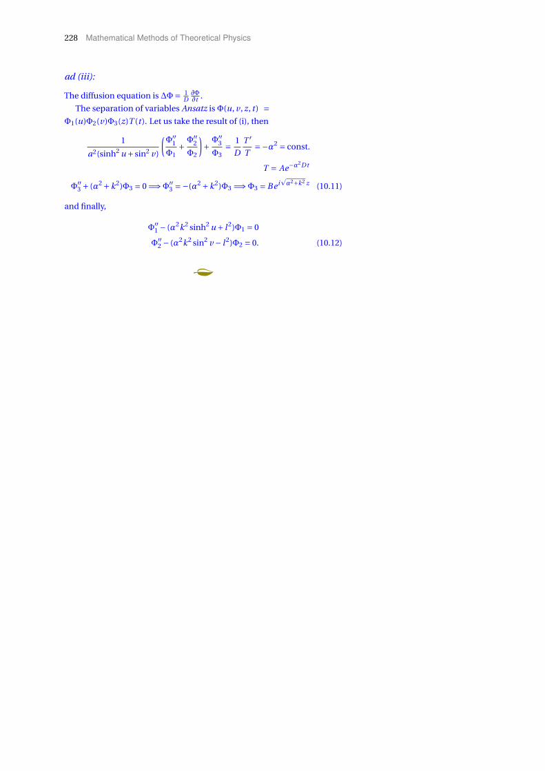
228 Mathematical Methods of Theoretical Physics

ad (iii):

The diffusion equation is ∆Φ= 1D∂Φ∂t .

The separation of variables Ansatz isΦ(u, v , z, t) =Φ1(u)Φ2(v)Φ3(z)T (t ). Let us take the result of (i), then

1

a2(sinh2 u + sin2 v)

(Φ′′

1

Φ1+ Φ

′′2

Φ2

)+ Φ

′′3

Φ3= 1

D

T ′

T=−α2 = const.

T = Ae−α2Dt

Φ′′3 + (α2 +k2)Φ3 = 0 =⇒Φ′′

3 =−(α2 +k2)Φ3 =⇒Φ3 = Be ipα2+k2 z (10.11)

and finally,

Φ′′1 − (α2k2 sinh2 u + l 2)Φ1 = 0

Φ′′2 − (α2k2 sin2 v − l 2)Φ2 = 0. (10.12)

g

Special functions of mathematical physics 229

11Special functions of mathematical physics

Special functions often arise as solutions of differential equations; This chapter follows several ap-proaches: N. N. Lebedev. Special Functionsand Their Applications. Prentice-HallInc., Englewood Cliffs, N.J., 1965. R.A. Silverman, translator and editor;reprinted by Dover, New York, 1972,Herbert S. Wilf. Mathematics for thephysical sciences. Dover, New York,1962. URL http://www.math.upenn.

edu/~wilf/website/Mathematics_

for_the_Physical_Sciences.html,W. W. Bell. Special Functions for Scien-tists and Engineers. D. Van NostrandCompany Ltd, London, 1968, George E.Andrews, Richard Askey, and RanjanRoy. Special Functions, volume 71 ofEncyclopedia of Mathematics and itsApplications. Cambridge University Press,Cambridge, 1999. ISBN 0-521-62321-9,Vadim Kuznetsov. Special functionsand their symmetries. Part I: Algebraicand analytic methods. PostgraduateCourse in Applied Analysis, May 2003.URL http://www1.maths.leeds.ac.

uk/~kisilv/courses/sp-funct.pdf

and Vladimir Kisil. Special functionsand their symmetries. Part II: Algebraicand symmetry methods. PostgraduateCourse in Applied Analysis, May 2003.URL http://www1.maths.leeds.ac.uk/

~kisilv/courses/sp-repr.pdf.

For reference, consider MiltonAbramowitz and Irene A. Stegun, edi-tors. Handbook of Mathematical Functionswith Formulas, Graphs, and Mathe-matical Tables. Number 55 in NationalBureau of Standards Applied Mathemat-ics Series. U.S. Government PrintingOffice, Washington, D.C., 1964. URLhttp://www.math.sfu.ca/~cbm/aands/,Yuri Alexandrovich Brychkov and Ana-tolii Platonovich Prudnikov. Handbookof special functions: derivatives, integrals,series and other formulas. CRC/Chapman& Hall Press, Boca Raton, London, NewYork, 2008 and I. S. Gradshteyn and I. M.Ryzhik. Tables of Integrals, Series, andProducts, 6th ed. Academic Press, SanDiego, CA, 2000.

for instance as eigenfunctions of differential operators in quantum

mechanics. Sometimes they occur after several separation of variables

and substitution steps have transformed the physical problem into

something manageable. For instance, we might start out with some

linear partial differential equation like the wave equation, then separate

the space from time coordinates, then separate the radial from the

angular components, and finally, separate the two angular parameters.

After we have done that, we end up with several separate differential

equations of the Liouville form; among them the Legendre differential

equation leading us to the Legendre polynomials.

In what follows, a particular class of special functions will be consid-

ered. These functions are all special cases of the hypergeometric function,

which is the solution of the hypergeometric differential equation. The

hypergeometric function exhibits a high degree of “plasticity,” as many

elementary analytic functions can be expressed by it.

First, as a prerequisite, let us define the gamma function. Then we

proceed to second order Fuchsian differential equations; followed by

rewriting a Fuchsian differential equation into a hypergeometric differen-

tial equation. Then we study the hypergeometric function as a solution

to the hypergeometric differential equation. Finally, we mention some

particular hypergeometric functions, such as the Legendre orthogonal

polynomials, and others.

Again, if not mentioned otherwise, we shall restrict our attention

to second order differential equations. Sometimes – such as for the

Fuchsian class – a generalization is possible but not very relevant for

physics.

11.1 Gamma function

The gamma function Γ(x) is an extension of the factorial (function)

n! because it generalizes the “classical” factorial, which is defined on

the natural numbers, to real or complex arguments (different from the

negative integers and from zero); that is,

Γ(n +1) = n! for n ∈N, or Γ(n) = (n −1)! for n ∈N−0. (11.1)

230 Mathematical Methods of Theoretical Physics

Let us first define the shifted factorial or, by another naming, the

Pochhammer symbol

(a)0def= 1,

(a)ndef= a(a +1) · · · (a +n −1), (11.2)

where n > 0 and a can be any real or complex number. If a is a natural

number greater than zero, (a)n = Γ(a+n)Γ(a) . Note that (a)1 = a and (a)2 =

a(a +1), and so on.

With this definition of the shifted factorial,

z!(z +1)n = 1 ·2 · · ·z · (z +1)((z +1)+1) · · · ((z +1)+n −1)

= 1 ·2 · · ·z · (z +1)(z +2) · · · (z +n)

= (z +n)!,

or z! = (z +n)!(z +1)n

. (11.3)

Since

(z +n)! = (n + z)!

= 1 ·2 · · ·n · (n +1)(n +2) · · · (n + z)

= n! · (n +1)(n +2) · · · (n + z)

= n!(n +1)z , (11.4)

we can rewrite Equation (11.3) into

z! = n!(n +1)z

(z +1)n= n!nz

(z +1)n

(n +1)z

nz . (11.5)

The latter factor, for large n, converges as Again, just as on page 161, “O(x)” means“of the order of x” or “absolutely boundby” in the following way: if g (x) is apositive function, then f (x) = O(g (x))implies that there exist a positive realnumber m such that | f (x)| < mg (x).

(n +1)z

nz = (n +1)((n +1)+1) · · · ((n +1)+ z −1)

nz

= (n +1)

n

(n +2)

n· · · (n + z)

n︸ ︷︷ ︸z factors

= nz +O(nz−1)

nz = nz

nz + O(nz−1)

nz = 1+O(n−1)n→∞−→ 1. (11.6)

In this limit, Equation (11.5) can be written as

z! = limn→∞z! = lim

n→∞n!nz

(z +1)n. (11.7)

Hence, for all z ∈ Cwhich are not equal to a negative integer – that is,

z 6∈ −1,−2, . . . – we can, in analogy to the “classical factorial,” define a

“factorial function shifted by one” as

Γ(z +1)def= lim

n→∞n!nz

(z +1)n. (11.8)

That is, Γ(z +1) has been redefined to allow an analytic continuation of the

“classical” factorial z! for z ∈ N: in (11.8) z just appears in an exponent

and in the argument of a shifted factorial.

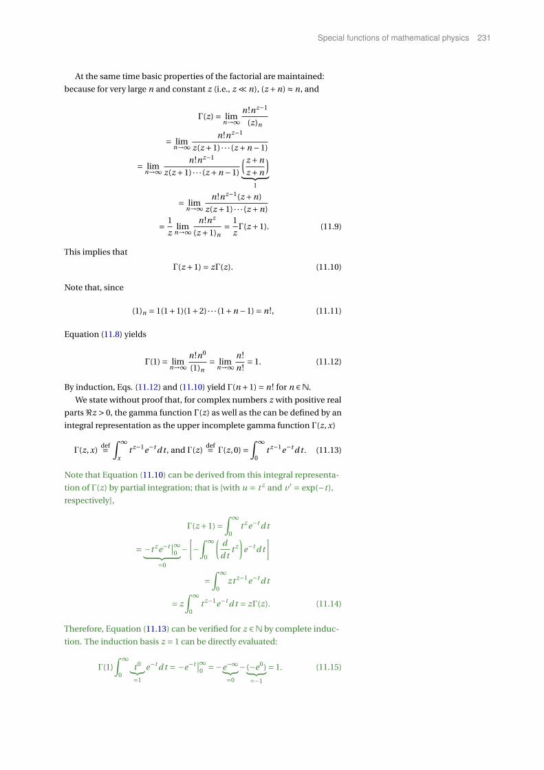
Special functions of mathematical physics 231

At the same time basic properties of the factorial are maintained:

because for very large n and constant z (i.e., z ¿ n), (z +n) ≈ n, and

Γ(z) = limn→∞

n!nz−1

(z)n

= limn→∞

n!nz−1

z(z +1) · · · (z +n −1)

= limn→∞

n!nz−1

z(z +1) · · · (z +n −1)

( z +n

z +n

)︸ ︷︷ ︸

1

= limn→∞

n!nz−1(z +n)

z(z +1) · · · (z +n)

= 1

zlim

n→∞n!nz

(z +1)n= 1

zΓ(z +1). (11.9)

This implies that

Γ(z +1) = zΓ(z). (11.10)

Note that, since

(1)n = 1(1+1)(1+2) · · · (1+n −1) = n!, (11.11)

Equation (11.8) yields

Γ(1) = limn→∞

n!n0

(1)n= lim

n→∞n!n!

= 1. (11.12)

By induction, Eqs. (11.12) and (11.10) yield Γ(n +1) = n! for n ∈N.

We state without proof that, for complex numbers z with positive real

parts ℜz > 0, the gamma function Γ(z) as well as the can be defined by an

integral representation as the upper incomplete gamma function Γ(z, x)

Γ(z, x)def=

∫ ∞

xt z−1e−t d t , and Γ(z)

def= Γ(z,0) =∫ ∞

0t z−1e−t d t . (11.13)

Note that Equation (11.10) can be derived from this integral representa-

tion of Γ(z) by partial integration; that is [with u = t z and v ′ = exp(−t),

respectively],

Γ(z +1) =∫ ∞

0t z e−t d t

= −t z e−t ∣∣∞0︸ ︷︷ ︸

=0

−[−

∫ ∞

0

(d

d tt z

)e−t d t

]

=∫ ∞

0zt z−1e−t d t

= z∫ ∞

0t z−1e−t d t = zΓ(z). (11.14)

Therefore, Equation (11.13) can be verified for z ∈N by complete induc-

tion. The induction basis z = 1 can be directly evaluated:

Γ(1)∫ ∞

0t 0︸︷︷︸=1

e−t d t = −e−t ∣∣∞0 =−e−∞︸︷︷︸

=0

− (−e0)︸ ︷︷ ︸=−1

= 1. (11.15)

232 Mathematical Methods of Theoretical Physics

We also mention the following formulæ:

Γ

(1

2

)=

∫ ∞

0

1pt

e−t d t

[variable substitution: u =pt , t = u2,d t = 2u du]

=∫ ∞

0

1

ue−u2

2u du = 2∫ ∞

0e−u2

du =∫ ∞

−∞e−u2

du =pπ, (11.16)

where the Gaussian integral (7.19) on page 177 has been used. Further-

more, more generally, without proof

Γ(n

2

)=p

π(n −2)!!2(n−1)/2

, for n > 0; and (11.17)

Euler’s reflection formula Γ(x)Γ(1−x) = π

sin(πx). (11.18)

Here, the double factorial is defined by

n!! =

1 if n =−1,0,

2 ·4 · · · (n −2) ·n for even n = 2k,k ∈N1 ·3 · · · (n −2) ·n for odd n = 2k −1,k ∈N.

(11.19)

Note that the even and odd cases can be respectively rewritten as

for even n = 2k,k ≥ 1 : n!! = 2 ·4 · · · (n −2) ·n

[n = 2k,k ∈N] = (2k)!! =k∏

i=1(2i ) = 2k

k∏i=1

i

= 2k ·1 ·2 · · · (k −1) ·k = 2k k!

for odd n = 2k −1,k ≥ 1 : n!! = 1 ·3 · · · (n −2) ·n

[n = 2k −1,k ∈N] = (2k −1)!! =k∏

i=1(2i −1)

= 1 ·3 · · · (2k −1)(2k)!!(2k)!!︸ ︷︷ ︸

=1

= 1 ·2 · · · (2k −2) · (2k −1) · (2k)

(2k)!!= (2k)!

2k k!

= k!(k +1)(k +2) · · · [(k +1)+k −2][(k +1)+k −1]

2k k!= (k +1)k

2k(11.20)

Stirling’s formula1 [again, O(x) means “of the order of x”] 1 Victor Namias. A simple derivation ofStirling’s asymptotic series. AmericanMathematical Monthly, 93:25–29, 041986. D O I : 10.2307/2322540. URLhttps://doi.org/10.2307/2322540

logn! = n logn −n +O(log(n)), or

n! n→∞−→ p2πn

(n

e

)n, or, more generally,

Γ(x) =√

2π

x

( x

e

)x(1+O

(1

x

))(11.21)

is stated without proof.

11.2 Beta function

The beta function, also called the Euler integral of the first kind, is a

special function defined by

B(x, y) =∫ 1

0t x−1(1− t )y−1d t = Γ(x)Γ(y)

Γ(x + y)for ℜx,ℜy > 0 (11.22)

Special functions of mathematical physics 233

No proof of the identity of the two representations in terms of an integral,

and of Γ-functions is given.

11.3 Fuchsian differential equations

Many differential equations of theoretical physics are Fuchsian equa-

tions. We shall, therefore, study this class in some generality.

11.3.1 Regular, regular singular, and irregular singular point

Consider the homogeneous differential equation [Equation (9.1) on page

217 is inhomogeneous]

Lx y(x) = a2(x)d 2

d x2 y(x)+a1(x)d

d xy(x)+a0(x)y(x) = 0. (11.23)

If a0(x), a1(x) and a2(x) are analytic at some point x0 and in its neigh-

borhood, and if a2(x0) 6= 0 at x0, then x0 is called an ordinary point, or

regular point. We state without proof that in this case the solutions

around x0 can be expanded as power series. In this case we can divide

equation (11.23) by a2(x) and rewrite it

1

a2(x)Lx y(x) = d 2

d x2 y(x)+p1(x)d

d xy(x)+p2(x)y(x) = 0, (11.24)

with p1(x) = a1(x)/a2(x) and p2(x) = a0(x)/a2(x).

If, however, a2(x0) = 0 and a1(x0) or a0(x0) are nonzero, then the x0 is

called singular point of (11.23). In the simplest case a2(x) has a simple

zero at x0: then both p1(x) and p2(x) in (11.24) have at most simple poles.

Furthermore, for reasons disclosed later – mainly motivated by the

possibility to write the solutions as power series – a point x0 is called a

regular singular point of Equation (11.23) if

limx→x0

[(x −x0)

a1(x)

a2(x)

]= lim

x→x0

[(x −x0)p1(x)

], as well as

limx→x0

[(x −x0)2 a0(x)

a2(x)

]= lim

x→x0

[(x −x0)2p2(x)

](11.25)

both exist. If anyone of these limits does not exist, the singular point is an

irregular singular point.

A linear ordinary differential equation is called Fuchsian, or Fuchsian

differential equation generalizable to arbitrary order n of differentiation[d n

d xn +p1(x)d n−1

d xn−1 +·· ·+pn−1(x)d

d x+pn(x)

]y(x) = 0, (11.26)

if every singular point, including infinity, is regular, meaning that pk (x)

has at most poles of order k.

A very important case is a Fuchsian of the second order (up to second

derivatives occur). In this case, we suppose that the coefficients in (11.24)

satisfy the following conditions:

• p1(x) has at most single poles, and

• p2(x) has at most double poles.

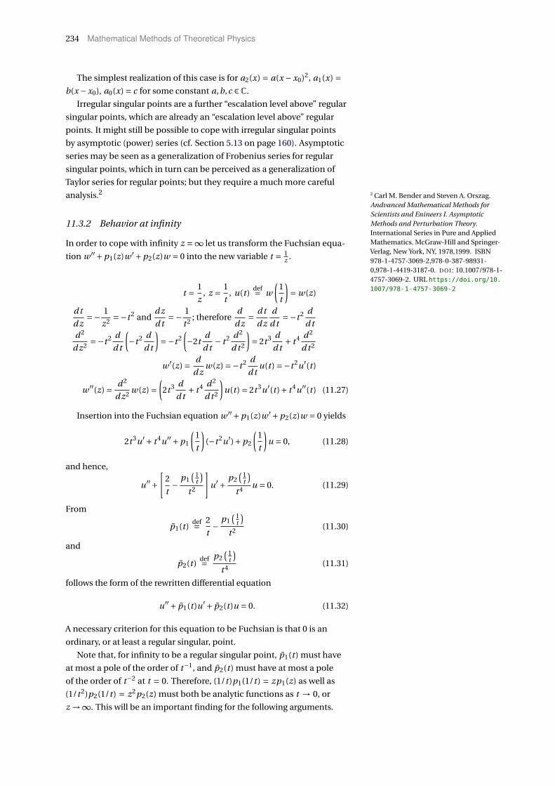
234 Mathematical Methods of Theoretical Physics

The simplest realization of this case is for a2(x) = a(x − x0)2, a1(x) =b(x −x0), a0(x) = c for some constant a,b,c ∈C.

Irregular singular points are a further “escalation level above” regular

singular points, which are already an “escalation level above” regular

points. It might still be possible to cope with irregular singular points

by asymptotic (power) series (cf. Section 5.13 on page 160). Asymptotic

series may be seen as a generalization of Frobenius series for regular

singular points, which in turn can be perceived as a generalization of

Taylor series for regular points; but they require a much more careful

analysis.2 2 Carl M. Bender and Steven A. Orszag.Andvanced Mathematical Methods forScientists and Enineers I. AsymptoticMethods and Perturbation Theory.International Series in Pure and AppliedMathematics. McGraw-Hill and Springer-Verlag, New York, NY, 1978,1999. ISBN978-1-4757-3069-2,978-0-387-98931-0,978-1-4419-3187-0. D O I : 10.1007/978-1-4757-3069-2. URL https://doi.org/10.

1007/978-1-4757-3069-2

11.3.2 Behavior at infinity

In order to cope with infinity z =∞ let us transform the Fuchsian equa-

tion w ′′+p1(z)w ′+p2(z)w = 0 into the new variable t = 1z .

t = 1

z, z = 1

t, u(t )

def= w

(1

t

)= w(z)

d t

d z=− 1

z2 =−t 2 andd z

d t=− 1

t 2 ; therefored

d z= d t

d z

d

d t=−t 2 d

d td 2

d z2 =−t 2 d

d t

(−t 2 d

d t

)=−t 2

(−2t

d

d t− t 2 d 2

d t 2

)= 2t 3 d

d t+ t 4 d 2

d t 2

w ′(z) = d

d zw(z) =−t 2 d

d tu(t ) =−t 2u′(t )

w ′′(z) = d 2

d z2 w(z) =(2t 3 d

d t+ t 4 d 2

d t 2

)u(t ) = 2t 3u′(t )+ t 4u′′(t ) (11.27)

Insertion into the Fuchsian equation w ′′+p1(z)w ′+p2(z)w = 0 yields

2t 3u′+ t 4u′′+p1

(1

t

)(−t 2u′)+p2

(1

t

)u = 0, (11.28)

and hence,

u′′+[

2

t− p1

( 1t

)t 2

]u′+ p2

( 1t

)t 4 u = 0. (11.29)

From

p1(t )def= 2

t− p1

( 1t

)t 2 (11.30)

and

p2(t )def= p2

( 1t

)t 4 (11.31)

follows the form of the rewritten differential equation

u′′+ p1(t )u′+ p2(t )u = 0. (11.32)

A necessary criterion for this equation to be Fuchsian is that 0 is an

ordinary, or at least a regular singular, point.

Note that, for infinity to be a regular singular point, p1(t) must have

at most a pole of the order of t−1, and p2(t) must have at most a pole

of the order of t−2 at t = 0. Therefore, (1/t)p1(1/t) = zp1(z) as well as

(1/t 2)p2(1/t) = z2p2(z) must both be analytic functions as t → 0, or

z →∞. This will be an important finding for the following arguments.

Special functions of mathematical physics 235

11.3.3 Functional form of the coefficients in Fuchsian differential

equations

The functional form of the coefficients p1(x) and p2(x), resulting from

the assumption of merely regular singular points can be estimated as

follows.

First, let us start with poles at finite complex numbers. Suppose there

are k finite poles. [The behavior of p1(x) and p2(x) at infinity will be

treated later.] Therefore, in Equation (11.24), the coefficients must be of

the form

p1(x) = P1(x)∏kj=1(x −x j )

,

and p2(x) = P2(x)∏kj=1(x −x j )2

, (11.33)

where the x1, . . . , xk are k the (regular singular) points of the poles, and

P1(x) and P2(x) are entire functions; that is, they are analytic (or, by

another wording, holomorphic) over the whole complex plane formed by

x | x ∈C.

Second, consider possible poles at infinity. Note that the requirement

that infinity is regular singular will restrict the possible growth of p1(x) as

well as p2(x) and thus, to a lesser degree, of P1(x) as well as P2(x).

As has been shown earlier, because of the requirement that infinity is

regular singular, as x approaches infinity, p1(x)x as well as p2(x)x2 must

both be analytic. Therefore, p1(x) cannot grow faster than |x|−1, and

p2(x) cannot grow faster than |x|−2.

Consequently, by (11.33), as x approaches infinity, P1(x) =p1(x)

∏kj=1(x − x j ) does not grow faster than |x|k−1 – which in turn

means that P1(x) is bounded by some constant times |x|k−1. Furthmore,

P2(x) = p2(x)∏k

j=1(x − x j )2 does not grow faster than |x|2k−2 – which in

turn means that P2(x) is bounded by some constant times |x|2k−2.

Recall that both P1(x) and P2(x) are entire functions. Therefore, be-

cause of the generalized Liouville theorem3 (mentioned on page 159),

3 Robert E. Greene and Stephen G.Krantz. Function theory of one complexvariable, volume 40 of Graduate Studiesin Mathematics. American MathematicalSociety, Providence, Rhode Island, thirdedition, 2006

both P1(x) and P2(x) must be polynomials of degree of at most k −1 and

2k −2, respectively.

Moreover, by using partial fraction decomposition4 of the rational

4 See also, for instance, Chapter 3,pp. 29-42, as well as Appendix C, p. 201of Gerhard Kristensson. Second OrderDifferential Equations. Springer, NewYork, 2010. ISBN 978-1-4419-7019-0. D O I : 10.1007/978-1-4419-7020-6.URL https://doi.org/10.1007/

978-1-4419-7020-6, and p. 146 of PeterHenrici. Applied and Computational Com-plex Analysis, Volume 2: Special Functions,Integral Transforms, Asymptotics, Contin-ued Fractions. John Wiley & Sons Inc, NewYork, 1977,1991. ISBN 978-0-471-54289-6.

For a particular example, considerx2+2x−18

x2+x−6, and first reduce the order

of the polynomial x2 + 2x − 18 in thenumerator by dividing it with the denom-inator x2 + x −6, resulting in 1+ x−12

x2+x−6.

Now suppose that the following Ansatzcould be made: x−12

x2+x−6= x−12

(x−2)(x+3) =A

x−2 + Bx+3 = A(x+3)

(x−2)(x+3) + B(x−2)(x−2)(x+3) .

Therefore, x −12 = A(x +3)+B(x −2). Bysubstituting x = 2 and x =−3 one obtainsA = −2 and B = 3, respectively. Hencex2+2x−18

x2+x−6= 1− 2

x−2 + 3x+3 .

functions – that is, the quotients R(x)Q(x) of polynomials R(x) and nonzero

Q(x) – in terms of their pole factors x − x j , we obtain from (11.33) the

general form of the coefficients

p1(x) =k∑

j=1

A j

x −x j,

and p2(x) =k∑

j=1

[B j

(x −x j )2 + C j

x −x j

], (11.34)

with constant A j ,B j ,C j ∈C. The resulting Fuchsian differential equation

is called Riemann differential equation.

Although we have considered an arbitrary finite number of poles, for

reasons that are unclear to this author, physics is mainly concerned with

two poles (i.e., k = 2) at finite points, and one at infinity.

236 Mathematical Methods of Theoretical Physics

The hypergeometric differential equation is a Fuchsian differential

equation which has at most three regular singularities, including infinity,

at5 0, 1, and ∞. 5 Vadim Kuznetsov. Special functionsand their symmetries. Part I: Algebraicand analytic methods. PostgraduateCourse in Applied Analysis, May 2003.URL http://www1.maths.leeds.ac.uk/

~kisilv/courses/sp-funct.pdf

11.3.4 Frobenius method: Solution by power series

Now let us get more concrete about the solution of Fuchsian equations.

Thereby the general strategy is to transform an ordinary differential

equation into a system of (coupled) linear equations as follows: It turns

out that the solutions of Fuchsian differential equations can be expanded

as power series, so that the differentiations can be performed explicitly.

The unknow coefficients of these power series which “encode the solu-

tions” are then obtained by utilizing the linear independence of different

powers in these series. Thereby every factor multiplied by the powers in

these series is enforced to vanish separately.

In order to obtain a feeling for power series solutions of differential

equations, consider the “first order” Fuchsian equation6 6 Ron Larson and Bruce H. Edwards.Calculus. Brooks/Cole Cengage Learning,Belmont, CA, nineth edition, 2010. ISBN978-0-547-16702-2

y ′−λy = 0. (11.35)

Make the Ansatz, also known as Frobenius method,7 that the solution can 7 George B. Arfken and Hans J. Weber.Mathematical Methods for Physicists.Elsevier, Oxford, sixth edition, 2005. ISBN0-12-059876-0;0-12-088584-0

be expanded into a power series of the form

y(x) =∞∑

j=0a j x j . (11.36)

Then, the second term of Equation (11.35) is −λ∑∞j=0 a j x j , whereas the

first term can be written as(d

d x

∞∑j=0

a j x j

)=

∞∑j=0

j a j x j−1 =∞∑

j=1j a j x j−1

=∞∑

m= j−1=0(m +1)am+1xm =

∞∑j=0

( j +1)a j+1x j . (11.37)

As a result the differential equation (11.35) can be written in terms of the

sums in (11.37) and (11.36):

∞∑j=0

( j +1)a j+1x j −λ( ∞∑

j=0a j x j

)=

∞∑j=0

x j [( j +1)a j+1 −λa j]= 0. (11.38)

Note that polynomials xi and x j of different degrees i 6= j are linearly

independent of each other, so the differences ( j +1)a j+1 −λa j in (11.38)

have to be zero for all j ≥ 0. Thus by comparing the coefficients of x j , for

n ≥ 0, in (11.37) and in λ times the sum (11.36) one obtains

( j +1)a j+1 =λa j , or

a j+1 =λa j

j +1= a0

λ j+1

( j +1)!; that is, a j = a0

λ j

j !. (11.39)

Therefore,

y(x) =∞∑

j=0a0λ j

j !x j = a0

∞∑j=0

(λx) j

j != a0eλx . (11.40)

In the Fuchsian case let us consider the following Frobenius Ansatz

to expand the solution as a generalized power series around a regular

Special functions of mathematical physics 237

singular point x0, which can be motivated by Equation (11.33), and by the

Laurent series expansion (5.29)–(5.30) on page 153:

p1(x) = A1(x)

x −x0=

∞∑j=0

α j (x −x0) j−1 for 0 < |x −x0| < r1,

p2(x) = A2(x)

(x −x0)2 =∞∑

j=0β j (x −x0) j−2 for 0 < |x −x0| < r2,

y(x) = (x −x0)σ∞∑

l=0(x −x0)l wl =

∞∑l=0

(x −x0)l+σwl , with w0 6= 0, (11.41)

where A1(x) = [(x − x0)a1(x)]/a2(x) and A2(x) = [(x − x0)2a0(x)]/a2(x).

Equation (11.24) then becomes

d 2

d x2 y(x)+p1(x)d

d xy(x)+p2(x)y(x) = 0,[

d 2

d x2 +∞∑

j=0α j (x −x0) j−1 d

d x+

∞∑j=0

β j (x −x0) j−2

] ∞∑l=0

wl (x −x0)l+σ = 0,

∞∑l=0

(l +σ)(l +σ−1)wl (x −x0)l+σ−2

+[ ∞∑

l=0(l +σ)wl (x −x0)l+σ−1

] ∞∑j=0

α j (x −x0) j−1

+[ ∞∑

l=0wl (x −x0)l+σ

] ∞∑j=0

β j (x −x0) j−2 = 0,

(x −x0)σ−2∞∑

l=0(x −x0)l

[(l +σ)(l +σ−1)wl

+(l +σ)wl

∞∑j=0

α j (x −x0) j +wl

∞∑j=0

β j (x −x0) j]= 0,

(x −x0)σ−2

[ ∞∑l=0

(l +σ)(l +σ−1)wl (x −x0)l

+∞∑

l=0(l +σ)wl

∞∑j=0

α j (x −x0)l+ j +∞∑

l=0wl

∞∑j=0

β j (x −x0)l+ j

]= 0.

Next, in order to reach a common power of (x −x0), we perform an index

identification in the second and third summands (where the order of

the sums change): l = m in the first summand, as well as an index shift

l + j = m, and thus j = m − l . Since l ≥ 0 and j ≥ 0, also m = l + j cannot

238 Mathematical Methods of Theoretical Physics

be negative. Furthermore, 0 ≤ j = m − l , so that l ≤ m.

(x −x0)σ−2

[ ∞∑l=0

(l +σ)(l +σ−1)wl (x −x0)l

+∞∑

j=0

∞∑l=0

(l +σ)wlα j (x −x0)l+ j

+∞∑

j=0

∞∑l=0

wlβ j (x −x0)l+ j

]= 0,

(x −x0)σ−2[ ∞∑

m=0(m +σ)(m +σ−1)wm(x −x0)m

+∞∑

m=0

m∑l=0

(l +σ)wlαm−l (x −x0)l+m−l

+∞∑

m=0

m∑l=0

wlβm−l (x −x0)l+m−l

]= 0,

(x −x0)σ−2 ∞∑

m=0(x −x0)m [(m +σ)(m +σ−1)wm

+m∑

l=0(l +σ)wlαm−l +

m∑l=0

wlβm−l

]= 0,

(x −x0)σ−2 ∞∑

m=0(x −x0)m [(m +σ)(m +σ−1)wm

+m∑

l=0wl

((l +σ)αm−l +βm−l

)]= 0. (11.42)

If we can divide this equation through (x −x0)σ−2 and exploit the linear

independence of the polynomials (x −x0)m , we obtain an infinite number

of equations for the infinite number of coefficients wm by requiring that

all the terms “inbetween” the [· · · ]–brackets in Equation (11.42) vanish

individually. In particular, for m = 0 and w0 6= 0,

(0+σ)(0+σ−1)w0 +w0((0+σ)α0 +β0

)= 0

f0(σ)def= σ(σ−1)+σα0 +β0 = 0. (11.43)

The radius of convergence of the solution will, in accordance with the

Laurent series expansion, extend to the next singularity.

Note that in Equation (11.43) we have defined f0(σ) which we will use

now. Furthermore, for successive m, and with the definition of

fk (σ)def= αkσ+βk , (11.44)

we obtain the sequence of linear equations

w0 f0(σ) = 0

w1 f0(σ+1)+w0 f1(σ) = 0,

w2 f0(σ+2)+w1 f1(σ+1)+w0 f2(σ) = 0,

...

wn f0(σ+n)+wn−1 f1(σ+n −1)+·· ·+w0 fn(σ) = 0. (11.45)

which can be used for an inductive determination of the coefficients wk .

Equation (11.43) is a quadratic equation σ2 +σ(α0 −1)+β0 = 0 for the

characteristic exponents

σ1,2 = 1

2

[1−α0 ±

√(1−α0)2 −4β0

](11.46)

Special functions of mathematical physics 239

We state without proof that, if the difference of the characteristic expo-

nents

σ1 −σ2 =√

(1−α0)2 −4β0 (11.47)

is nonzero and not an integer, then the two solutions found from σ1,2

through the generalized series Ansatz (11.41) are linear independent.

Intuitively speaking, the Frobenius method “is in obvious trouble”

to find the general solution of the Fuchsian equation if the two charac-

teristic exponents coincide (e.g., σ1 = σ2), but it “is also in trouble” to

find the general solution if σ1 −σ2 = m ∈N; that is, if, for some positive

integer m, σ1 = σ2 +m > σ2. Because in this case, “eventually” at n = m

in Equation (11.45), we obtain as iterative solution for the coefficient wm

the term

wm =−wm−1 f1(σ2 +m −1)+·· ·+w0 fm(σ2)

f0(σ2 +m)

=−wm−1 f1(σ1 −1)+·· ·+w0 fm(σ2)

f0(σ1)︸ ︷︷ ︸=0

. (11.48)

That is, the greater critical exponent σ1 = σ2 +m is a solution of Equa-

tion (11.43) so that f0(σ1) in the denominator vanishes.

In these cases the greater characteristic exponent σ1 ≥ σ2 can still

be used to find a solution in terms of a power series, but the smaller

characteristic exponent σ2 in general cannot.

11.3.5 d’Alembert reduction of order

If σ1 = σ2 +n with n ∈ Z, then we find only a single solution of the

Fuchsian equation in terms of the power series resulting from inserting

the greater (or equal) characteristic exponent. In order to obtain another

linear independent solution we have to employ a method based on the

Wronskian,8 or the d’Alembert reduction,9 which is a general method

8 George B. Arfken and Hans J. Weber.Mathematical Methods for Physicists.Elsevier, Oxford, sixth edition, 2005. ISBN0-12-059876-0;0-12-088584-0

9 Gerald Teschl. Ordinary DifferentialEquations and Dynamical Systems.Graduate Studies in Mathematics, volume140. American Mathematical Society,Providence, Rhode Island, 2012. ISBNISBN-10: 0-8218-8328-3 / ISBN-13: 978-0-8218-8328-0. URL http://www.mat.

univie.ac.at/~gerald/ftp/book-ode/

ode.pdfto obtain another, linear independent solution y2(x) from an existing

particular solution y1(x) by the Ansatz (no proof is presented here)

y2(x) = y1(x)∫

xv(s)d s. (11.49)

240 Mathematical Methods of Theoretical Physics

Inserting y2(x) from (11.49) into the Fuchsian equation (11.24), and using

the fact that by assumption y1(x) is a solution of it, yields

d 2

d x2 y2(x)+p1(x)d

d xy2(x)+p2(x)y2(x) = 0,

d 2

d x2 y1(x)∫

xv(s)d s +p1(x)

d

d xy1(x)

∫x

v(s)d s +p2(x)y1(x)∫

xv(s)d s = 0,

d

d x

[d

d xy1(x)

]∫x

v(s)d s + y1(x)v(x)

+p1(x)

[d

d xy1(x)

]∫x

v(s)d s +p1(x)v(x)+p2(x)y1(x)∫

xv(s)d s = 0,[

d 2

d x2 y1(x)

]∫x

v(s)d s +[

d

d xy1(x)

]v(x)+

[d

d xy1(x)

]v(x)+ y1(x)

[d

d xv(x)

]+p1(x)

[d

d xy1(x)

]∫x

v(s)d s +p1(x)y1(x)v(x)+p2(x)y1(x)∫

xv(s)d s = 0,[

d 2

d x2 y1(x)

]∫x

v(s)d s +p1(x)

[d

d xy1(x)

]∫x

v(s)d s +p2(x)y1(x)∫

xv(s)d s

+p1(x)y1(x)v(x)+[

d

d xy1(x)

]v(x)+

[d

d xy1(x)

]v(x)+ y1(x)

[d

d xv(x)

]= 0,[

d 2

d x2 y1(x)

]∫x

v(s)d s +p1(x)

[d

d xy1(x)

]∫x

v(s)d s +p2(x)y1(x)∫

xv(s)d s

+y1(x)

[d

d xv(x)

]+2

[d

d xy1(x)

]v(x)+p1(x)y1(x)v(x) = 0,[

d 2

d x2 y1(x)

]+p1(x)

[d

d xy1(x)

]+p2(x)y1(x)

︸ ︷︷ ︸

=0

∫x

v(s)d s

+y1(x)

[d

d xv(x)

]+

2

[d

d xy1(x)

]+p1(x)y1(x)

v(x) = 0,

y1(x)

[d

d xv(x)

]+

2

[d

d xy1(x)

]+p1(x)y1(x)

v(x) = 0,

and finally,

v ′(x)+ v(x)

2

y ′1(x)

y1(x)+p1(x)

= 0. (11.50)

11.3.6 Computation of the characteristic exponent

Let w ′′+p1(z)w ′+p2(z)w = 0 be a Fuchsian equation. From the Laurent

series expansion of p1(z) and p2(z) in (11.41) and Cauchy’s integral

formula we can derive the following equations, which are helpful in

determining the characteristic exponent σ, as defined in (11.43) by

σ(σ−1)+σα0 +β0 = 0:

α0 = limz→z0

(z − z0)p1(z),

β0 = limz→z0

(z − z0)2p2(z), (11.51)

where z0 is a regular singular point.

In order to find α0, consider the Laurent series for

p1(z) =∞∑

k=−1ak (z − z0)k ,

with ak = 1

2πi

∮p1(s)(s − z0)−(k+1)d s. (11.52)

Special functions of mathematical physics 241

The summands vanish for k < −1, because p1(z) has at most a pole of

order one at z0.

An index change n = k + 1, or k = n − 1, as well as a redefinition

αndef= an−1 yields

p1(z) =∞∑

n=0αn(z − z0)n−1, (11.53)

where

αn = an−1 = 1

2πi

∮p1(s)(s − z0)−nd s; (11.54)

and, in particular,

α0 = 1

2πi

∮p1(s)d s. (11.55)

Because the equation is Fuchsian, p1(z) has at most a pole of order one at

z0. Therefore, (z − z0)p1(z) is analytic around z0. By multiplying p1(z) with

unity 1 = (z − z0)/(z − z0) and insertion into (11.55) we obtain

α0 = 1

2πi

∮p1(s)(s − z0)

(s − z0)d s. (11.56)

Cauchy’s integral formula (5.21) on page 151 yields

α0 = lims→z0

p1(s)(s − z0). (11.57)

Alternatively we may consider the Frobenius Ansatz (11.41) p1(z) =∑∞n=0αn(z − z0)n−1 which has again been motivated by the fact that p1(z)

has at most a pole of order one at z0. Multiplication of this series by (z −z0)

yields

(z − z0)p1(z) =∞∑

n=0αn(z − z0)n . (11.58)

In the limit z → z0,

α0 = limz→z0

(z − z0)p1(z). (11.59)

Likewise, let us find the expression for β0 by considering the Laurent

series for

p2(z) =∞∑

k=−2bk (z − z0)k

with bk = 1

2πi

∮p2(s)(s − z0)−(k+1)d s. (11.60)

The summands vanish for k < −2, because p2(z) has at most a pole of

order two at z0.

An index change n = k + 2, or k = n − 2, as well as a redefinition

βndef= bn−2 yields

p2(z) =∞∑

n=0βn(z − z0)n−2, (11.61)

where

βn = bn−2 = 1

2πi

∮p2(s)(s − z0)−(n−1)d s; (11.62)

and, in particular,

β0 = 1

2πi

∮(s − z0)p2(s)d s. (11.63)

242 Mathematical Methods of Theoretical Physics

Because the equation is Fuchsian, p2(z) has at most a pole of order

two at z0. Therefore, (z − z0)2p2(z) is analytic around z0. By multiplying

p2(z) with unity 1 = (z − z0)2/(z − z0)2 and insertion into (11.63) we obtain

β0 = 1

2πi

∮p2(s)(s − z0)2

(s − z0)d s. (11.64)

Cauchy’s integral formula (5.21) on page 151 yields

β0 = lims→z0

p2(s)(s − z0)2. (11.65)

Again another way to see this is with the Frobenius Ansatz (11.41)

p2(z) = ∑∞n=0βn(z − z0)n−2. Multiplication with (z − z0)2, and taking the

limit z → z0, yields

limz→z0

(z − z0)2p2(z) =βn . (11.66)

11.3.7 Examples

Let us consider some examples involving Fuchsian equations of the

second order.

1. First, we shall prove that z2 y ′′(z)+ z y ′(z)− y(z) = 0 is of the Fuchsian

type, and compute the solutions with the Frobenius method.

Let us first locate the singularities of

y ′′(z)+ y ′(z)

z− y(z)

z2 = 0. (11.67)

One singularity is at the (finite) point z0 = 0.

In order to analyze the singularity at infinity, we have to transform the

equation by z = 1/t . First observe that p1(z) = 1/z and p2(z) =−1/z2.

Therefore, after the transformation, the new coefficients, computed

from (11.30) and (11.31), are

p1(t ) =(

2

t− t

t 2

)= 1

t, and

p2(t ) = −t 2

t 4 =− 1

t 2 . (11.68)

Thereby we effectively regain the original type of equation (11.67). We

can thus treat both singularities at zero and infinity in the same way.

Both singularities are regular, as the coefficients p1 and p1 have poles

of order 1, p2 and p2 have poles of order 2, respectively. Therefore, the

differential equation is Fuchsian.

In order to obtain solutions, let us first compute the characteristic

exponents by

α0 = limz→0

zp1(z) = limz→0

z1

z= 1, and

β0 = limz→0

z2p2(z) = limz→0

−z2 1

z2 =−1, (11.69)

so that, from (11.43),

0 = f0(σ) =σ(σ−1)+σα0 +β0 =σ2 −σ+σ−1 ==σ2 −1, and thus σ1,2 =±1. (11.70)

Special functions of mathematical physics 243

The first solution is obtained by insertion of the Frobenius

Ansatz (11.41), in particular, y1(x) = ∑∞l=0(x − x0)l+σwl with σ1 = 1

and x0 = 0 into (11.67). In this case,

x2∞∑

l=0(l +1)l x l−1wl +x

∞∑l=0

(l +1)x l wl −∞∑

l=0x l+1wl = 0,

∞∑l=0

[(l +1)l + (l +1)−1] x l+1wl =∞∑

l=0wl l (l +2)x l+1 = 0. (11.71)

Since the polynomials are linear independent, we obtain wl l (l +2) = 0

for all l ≥ 0. Therefore, for constant A,

w0 = A, and wl = 0 for l > 0. (11.72)

So, the first solution is y1(z) = Az.

The second solution, computed through the Frobenius Ansatz (11.41),

is obtained by inserting y2(x) = ∑∞l=0(x − x0)l+σwl with σ2 = −1 into

(11.67). This yields

z2∞∑

l=0(l −1)(l −2)(x −x0)l−3wl+

+z∞∑

l=0(l −1)(x −x0)l−2wl −

∞∑l=0

(x −x0)l−1wl = 0,

∞∑l=0

[wl (l −1)(l −2)+wl (l −1)−wl ] (x −x0)l−1wl = 0,

∞∑l=0

wl l (l −2)(x −x0)l−1 = 0. (11.73)

Since the polynomials are linear independent, we obtain wl l (l −2) = 0

for all l ≥ 0. Therefore, for constant B ,C ,

w0 = B , w1 = 0, w2 =C , and wl = 0 for l > 2, (11.74)

So that the second solution is y2(z) = B 1z +C z.

Note that y2(z) already represents the general solution of (11.67). Al- Most of the coefficients are zero, so noiteration with a “catastrophic divisions byzero” occurs here.

ternatively we could have started from y1(z) and applied d’Alembert’s

Ansatz (11.49)–(11.50):

v ′(z)+ v(z)

(2

z+ 1

z

)= 0, or v ′(z) =−3v(z)

z(11.75)

yields

d v

v=−3

d z

z, and log v =−3log z, or v(z) = z−3. (11.76)

Therefore, according to (11.49),

y2(z) = y1(z)∫

zv(s)d s = Az

(− 1

2z2

)= A′

z. (11.77)

2. Find out whether the following differential equations are Fuchsian,

and enumerate the regular singular points:

zw ′′+ (1− z)w ′ = 0,

z2w ′′+ zw ′−ν2w = 0,

z2(1+ z)2w ′′+2z(z +1)(z +2)w ′−4w = 0,

2z(z +2)w ′′+w ′− zw = 0. (11.78)

244 Mathematical Methods of Theoretical Physics

ad 1: zw ′′+ (1− z)w ′ = 0 =⇒ w ′′+ (1− z)

zw ′ = 0

z = 0:

α0 = limz→0

z(1− z)

z= 1, β0 = lim

z→0z2 ·0 = 0.

The equation for the characteristic exponent is

σ(σ−1)+σα0 +β0 = 0 =⇒σ2 −σ+σ= 0 =⇒σ1,2 = 0.

z =∞: z = 1t

p1(t ) = 2

t−

(1− 1

t

)1t

t 2 = 2

t−

(1− 1

t

)t

= 1

t+ 1

t 2 = t +1

t 2

=⇒ not Fuchsian.

ad 2: z2w ′′+ zw ′− v2w = 0 =⇒ w ′′+ 1

zw ′− v2

z2 w = 0.

z = 0:

α0 = limz→0

z1

z= 1, β0 = lim

z→0z2

(−v2

z2

)=−v2.

=⇒σ2 −σ+σ− v2 = 0 =⇒σ1,2 =±v

z =∞: z = 1t

p1(t ) = 2

t− 1

t 2 t = 1

t

p2(t ) = 1

t 4

(−t 2v2)=−v2

t 2

=⇒ u′′+ 1

tu′− v2

t 2 u = 0 =⇒σ1,2 =±v

=⇒ Fuchsian equation.

ad 3:

z2(1+z)2w ′′+2z(z+1)(z+2)w ′−4w = 0 =⇒ w ′′+2(z +2)

z(z +1)w ′− 4

z2(1+ z)2 w = 0

z = 0:

α0 = limz→0

z2(z +2)

z(z +1)= 4, β0 = lim

z→0z2

(− 4

z2(1+ z)2

)=−4.

=⇒σ(σ−1)+4σ−4 =σ2 +3σ−4 = 0 =⇒σ1,2 = −3±p9+16

2=

−4

+1

z =−1:

α0 = limz→−1

(z +1)2(z +2)

z(z +1)=−2, β0 = lim

z→−1(z +1)2

(− 4

z2(1+ z)2

)=−4.

=⇒σ(σ−1)−2σ−4 =σ2 −3σ−4 = 0 =⇒σ1,2 = 3±p9+16

2=

+4

−1

Special functions of mathematical physics 245

z =∞:

p1(t ) = 2

t− 1

t 2

2( 1

t +2)

1t

( 1t +1

) = 2

t− 2

( 1t +2

)1+ t

= 2

t

(1− 1+2t

1+ t

)

p2(t ) = 1

t 4

− 41t 2

(1+ 1

t

)2

=− 4

t 2

t 2

(t +1)2 =− 4

(t +1)2

=⇒ u′′+ 2

t

(1− 1+2t

1+ t

)u′− 4

(t +1)2 u = 0

α0 = limt→0

t2

t

(1− 1+2t

1+ t

)= 0, β0 = lim

t→0t 2

(− 4

(t +1)2

)= 0.

=⇒σ(σ−1) = 0 =⇒σ1,2 =

0

1

=⇒ Fuchsian equation.

ad 4:

2z(z +2)w ′′+w ′− zw = 0 =⇒ w ′′+ 1

2z(z +2)w ′− 1

2(z +2)w = 0

z = 0:

α0 = limz→0

z1

2z(z +2)= 1

4, β0 = lim

z→0z2 −1

2(z +2)= 0.

=⇒σ2 −σ+ 1

4σ= 0 =⇒σ2 − 3

4σ= 0 =⇒σ1 = 0,σ2 = 3

4.

z =−2:

α0 = limz→−2

(z +2)1

2z(z +2)=−1

4, β0 = lim

z→−2(z +2)2 −1

2(z +2)= 0.

=⇒σ1 = 0, σ2 = 5

4.

z =∞:

p1(t ) = 2

t− 1

t 2

(1

2 1t

( 1t +2

))= 2

t− 1

2(1+2t )

p2(t ) = 1

t 4

(−1)

2( 1

t +2) =− 1

2t 3(1+2t )

=⇒ not a Fuchsian.

3. Determine the solutions of

z2w ′′+ (3z +1)w ′+w = 0

around the regular singular points.

The singularities are at z = 0 and z =∞.

Singularities at z = 0:

p1(z) = 3z +1

z2 = a1(z)

zwith a1(z) = 3+ 1

z

p1(z) has a pole of higher order than one; hence this is no Fuchsian

equation; and z = 0 is an irregular singular point.

Singularities at z =∞:

246 Mathematical Methods of Theoretical Physics

• Transformation z = 1

t, w(z) → u(t ):

u′′(t )+[

2

t− 1

t 2 p1

(1

t

)]·u′(t )+ 1

t 4 p2

(1

t

)·u(t ) = 0.

The new coefficient functions are

p1(t ) = 2

t− 1

t 2 p1

(1

t

)= 2

t− 1

t 2 (3t + t 2) = 2

t− 3

t−1 =−1

t−1

p2(t ) = 1

t 4 p2

(1

t

)= t 2

t 4 = 1

t 2

• check whether this is a regular singular point:

p1(t ) =−1+ t

t= a1(t )

twith a1(t ) =−(1+ t ) regular

p2(t ) = 1

t 2 = a2(t )

t 2 with a2(t ) = 1 regular

a1 and a2 are regular at t = 0, hence this is a regular singular point.

• Ansatz around t = 0: the transformed equation is

u′′(t )+ p1(t )u′(t )+ p2(t )u(t ) = 0

u′′(t )−(

1

t+1

)u′(t )+ 1

t 2 u(t ) = 0

t 2u′′(t )− (t + t 2)u′(t )+u(t ) = 0

The generalized power series is

u(t ) =∞∑

n=0wn t n+σ

u′(t ) =∞∑

n=0wn(n +σ)t n+σ−1

u′′(t ) =∞∑

n=0wn(n +σ)(n +σ−1)t n+σ−2

If we insert this into the transformed differential equation we

obtain

t 2∞∑

n=0wn(n +σ)(n +σ−1)t n+σ−2−

− (t + t 2)∞∑

n=0wn(n +σ)t n+σ−1 +

∞∑n=0

wn t n+σ = 0

∞∑n=0

wn(n +σ)(n +σ−1)t n+σ−∞∑

n=0wn(n +σ)t n+σ−

−∞∑

n=0wn(n +σ)t n+σ+1 +

∞∑n=0

wn t n+σ = 0

Change of index: m = n +1, n = m −1 in the third sum yields

∞∑n=0

wn

[(n +σ)(n +σ−2)+1

]t n+σ−

∞∑m=1

wm−1(m −1+σ)t m+σ = 0.

In the second sum, substitute m for n

∞∑n=0

wn

[(n +σ)(n +σ−2)+1

]t n+σ−

∞∑n=1

wn−1(n +σ−1)t n+σ = 0.

Special functions of mathematical physics 247

We write out explicitly the n = 0 term of the first sum

w0

[σ(σ−2)+1

]tσ+

∞∑n=1

wn

[(n +σ)(n +σ−2)+1

]t n+σ

−∞∑

n=1wn−1(n +σ−1)t n+σ = 0.

The two sums can be combined

w0

[σ(σ−2)+1

]tσ

+∞∑

n=1

wn

[(n +σ)(n +σ−2)+1

]−wn−1(n +σ−1)

t n+σ = 0.

The left hand side can only vanish for all t if the coefficients vanish;

hence

w0

[σ(σ−2)+1

]= 0, (11.79)

wn

[(n +σ)(n +σ−2)+1

]−wn−1(n +σ−1) = 0. (11.80)

ad (11.79) for w0:

σ(σ−2)+1 = 0

σ2 −2σ+1 = 0

(σ−1)2 = 0 =⇒ σ(1,2)∞ = 1

The characteristic exponent is σ(1)∞ =σ(2)∞ = 1.

ad (11.80) for wn : For the coefficients wn we obtain the recursion

formula

wn

[(n +σ)(n +σ−2)+1

]= wn−1(n +σ−1)

=⇒ wn = n +σ−1

(n +σ)(n +σ−2)+1wn−1.

Let us insert σ= 1:

wn = n

(n +1)(n −1)+1wn−1 = n

n2 −1+1wn−1 = n

n2 wn−1 = 1

nwn−1.

We can fix w0 = 1, hence:

w0 = 1 = 1

1= 1

0!

w1 = 1

1= 1

1!

w2 = 1

1 ·2= 1

2!

w3 = 1

1 ·2 ·3= 1

3!...

wn = 1

1 ·2 ·3 · · · · ·n= 1

n!

And finally,

u1(t ) = tσ∞∑

n=0wn t n = t

∞∑n=0

t n

n!= te t .

248 Mathematical Methods of Theoretical Physics

• Notice that both characteristic exponents are equal; hence we have

to employ the d’Alembert reduction

u2(t ) = u1(t )

t∫0

v(s)d s

with

v ′(t )+ v(t )

[2

u′1(t )

u1(t )+ p1(t )

]= 0.

Insertion of u1 and p1,

u1(t ) = te t

u′1(t ) = e t (1+ t )

p1(t ) = −(

1

t+1

),

yields

v ′(t )+ v(t )

(2

e t (1+ t )

te t − 1

t−1

)= 0

v ′(t )+ v(t )

(2

(1+ t )

t− 1

t−1

)= 0

v ′(t )+ v(t )

(2

t+2− 1

t−1

)= 0

v ′(t )+ v(t )

(1

t+1

)= 0

d v

d t= −v

(1+ 1

t

)d v

v= −

(1+ 1

t

)d t

Upon integration of both sides we obtain∫d v

v= −

∫ (1+ 1

t

)d t

log v = −(t + log t ) =−t − log t

v = exp(−t − log t ) = e−t e− log t = e−t

t,

and hence an explicit form of v(t ):

v(t ) = 1

te−t .

If we insert this into the equation for u2 we obtain

u2(t ) = te t∫ t

0

1

se−s d s.

• Therefore, with t = 1z , u(t) = w(z), the two linear independent

solutions around the regular singular point at z =∞ are

w1(z) = 1

zexp

(1

z

), and

w2(z) = 1

zexp

(1

z

) 1z∫

0

1

te−t d t . (11.81)

Special functions of mathematical physics 249

11.4 Hypergeometric function

11.4.1 Definition

A hypergeometric series is a series

∞∑j=0

c j , (11.82)

where the quotientsc j+1

c jare rational functions (that is, the quotient of

two polynomials R(x)Q(x) , where Q(x) is not identically zero) of j , so that they

can be factorized:

c j+1

c j= ( j +a1)( j +a2) · · · ( j +ap )

( j +b1)( j +b2) · · · ( j +bq )

(x

j +1

),

or c j+1 = c j( j +a1)( j +a2) · · · ( j +ap )

( j +b1)( j +b2) · · · ( j +bq )

(x

j +1

)= c j−1

( j −1+a1)( j −1+a2) · · · ( j −1+ap )

( j −1+b1)( j −1+b2) · · · ( j −1+bq )

× ( j +a1)( j +a2) · · · ( j +ap )

( j +b1)( j +b2) · · · ( j +bq )

(x

j

)(x

j +1

)= c0

a1a2 · · ·ap

b1b2 · · ·bq· · · ( j −1+a1)( j −1+a2) · · · ( j −1+ap )

( j −1+b1)( j −1+b2) · · · ( j −1+bq )

× ( j +a1)( j +a2) · · · ( j +ap )

( j +b1)( j +b2) · · · ( j +bq )

( x

1

)· · ·

(x

j

)(x

j +1

)= c0

(a1) j+1(a2) j+1 · · · (ap ) j+1

(b1) j+1(b2) j+1 · · · (bq ) j+1

(x j+1

( j +1)!

). (11.83)

The factor j + 1 in the denominator of the first line of (11.83) on the

right yields ( j +1)!. If it were not there “naturally” we may obtain it by

compensation with a factor j +1 in the numerator.

With this iterated ratio (11.83), the hypergeometric series (11.82)

can be written in terms of shifted factorials, or, by another naming, the

Pochhammer symbol, as

∞∑j=0

c j = c0

∞∑j=0

(a1) j (a2) j · · · (ap ) j

(b1) j (b2) j · · · (bq ) j

x j

j !

= c0p Fq

(a1, . . . , ap

b1, . . . ,bq; x

), or

= c0p Fq(a1, . . . , ap ;b1, . . . ,bq ; x

). (11.84)

Apart from this definition via hypergeometric series, the Gauss hyper-

geometric function, or, used synonymously, the Gauss series

2F1

(a,b

c; x

)= 2F1 (a,b;c; x) =

∞∑j=0

(a) j (b) j

(c) j

x j

j !

= 1+ ab

cx + 1

2!a(a +1)b(b +1)

c(c +1)x2 +·· · (11.85)

can be defined as a solution of a Fuchsian differential equation which has

at most three regular singularities at 0, 1, and ∞.

Indeed, any Fuchsian equation with finite regular singularities at x1

and x2 can be rewritten into the Riemann differential equation (11.34),

250 Mathematical Methods of Theoretical Physics

which in turn can be rewritten into the Gaussian differential equation or

hypergeometric differential equation with regular singularities at 0, 1, and

∞.10 This can be demonstrated by rewriting any such equation of the

10 Einar Hille. Lectures on ordinarydifferential equations. Addison-Wesley,Reading, Mass., 1969; Garrett Birkhoff andGian-Carlo Rota. Ordinary DifferentialEquations. John Wiley & Sons, New York,Chichester, Brisbane, Toronto, fourthedition, 1959, 1960, 1962, 1969, 1978, and1989; and Gerhard Kristensson. SecondOrder Differential Equations. Springer,New York, 2010. ISBN 978-1-4419-7019-0. D O I : 10.1007/978-1-4419-7020-6.URL https://doi.org/10.1007/

978-1-4419-7020-6

The Bessel equation has a regular singularpoint at 0, and an irregular singular pointat infinity.

form

w ′′(x)+(

A1

x −x1+ A2

x −x2

)w ′(x)

+(

B1

(x −x1)2 + B2

(x −x2)2 + C1

x −x1+ C2

x −x2

)w(x) = 0 (11.86)

through transforming Equation (11.86) into the hypergeometric differen-

tial equation

[d 2

d x2 + (a +b +1)x − c

x(x −1)

d

d x+ ab

x(x −1)

]2F1(a,b;c; x) = 0, (11.87)

where the solution is proportional to the Gauss hypergeometric function

w(x) −→ (x −x1)σ(1)1 (x −x2)σ

(2)2 2F1(a,b;c; x), (11.88)

and the variable transform as

x −→ x = x −x1

x2 −x1, with

a =σ(1)1 +σ(1)

2 +σ(1)∞ ,

b =σ(1)1 +σ(1)

2 +σ(2)∞ ,

c = 1+σ(1)1 −σ(2)

1 . (11.89)

where σ(i )j stands for the i th characteristic exponent of the j th singular-

ity.

Whereas the full transformation from Equation (11.86) to the hyperge-

ometric differential equation (11.87) will not been given, we shall show

that the Gauss hypergeometric function 2F1 satisfies the hypergeometric

differential equation (11.87).

First, define the differential operator

ϑ= xd

d x, (11.90)

and observe that

ϑ(ϑ+ c −1)xn = xd

d x

(x

d

d x+ c −1

)xn

= xd

d x

(xnxn−1 + cxn −xn)

= xd

d x

(nxn + cxn −xn)

= xd

d x(n + c −1) xn

= n (n + c −1) xn . (11.91)

Special functions of mathematical physics 251

Thus, if we apply ϑ(ϑ+ c −1) to 2F1, then

ϑ(ϑ+ c −1) 2F1(a,b;c; x) =ϑ(ϑ+ c −1)∞∑

j=0

(a) j (b) j

(c) j

x j

j !

=∞∑

j=0

(a) j (b) j

(c) j

j ( j + c −1)x j

j !=

∞∑j=1

(a) j (b) j

(c) j

j ( j + c −1)x j

j !

=∞∑

j=1

(a) j (b) j

(c) j

( j + c −1)x j

( j −1)!

[index shift: j → n +1,n = j −1,n ≥ 0]

=∞∑

n=0

(a)n+1(b)n+1

(c)n+1

(n +1+ c −1)xn+1

n!

= x∞∑

n=0

(a)n(a +n)(b)n(b +n)

(c)n(c +n)

(n + c)xn

n!

= x∞∑

n=0

(a)n(b)n

(c)n

(a +n)(b +n)xn

n!

= x(ϑ+a)(ϑ+b)∞∑

n=0

(a)n(b)n

(c)n

xn

n!= x(ϑ+a)(ϑ+b) 2F1(a,b;c; x), (11.92)

where we have used

(a +n)xn = (a +ϑ)xn , and

(a)n+1 = a(a +1) · · · (a +n −1)(a +n) = (a)n(a +n). (11.93)

Writing out ϑ in Equation (11.92) explicitly yields

ϑ(ϑ+ c −1)−x(ϑ+a)(ϑ+b) 2F1(a,b;c; x) = 0,x

d

d x

(x

d

d x+ c −1

)−x

(x

d

d x+a

)(x

d

d x+b

)2F1(a,b;c; x) = 0,

d

d x

(x

d

d x+ c −1

)−

(x

d

d x+a

)(x

d

d x+b

)2F1(a,b;c; x) = 0,

d

d x+x

d 2

d x2 + (c −1)d

d x−

(x2 d 2

d x2 +xd

d x+bx

d

d x

+axd

d x+ab

)2F1(a,b;c; x) = 0,(

x −x2) d 2

d x2 + (1+ c −1−x −x(a +b))d

d x+ab

2F1(a,b;c; x) = 0,

−x(x −1)d 2

d x2 − (c −x(1+a +b))d

d x−ab

2F1(a,b;c; x) = 0,

d 2

d x2 + x(1+a +b)− c

x(x −1)

d

d x+ ab

x(x −1)

2F1(a,b;c; x) = 0.

(11.94)

11.4.2 Properties

There exist many properties of the hypergeometric series. In the follow-

ing, we shall mention a few.

d

d z2F1(a,b;c; z) = ab

c2F1(a +1,b +1;c +1; z). (11.95)

252 Mathematical Methods of Theoretical Physics

d

d z2F1(a,b;c; z) = d

d z

∞∑n=0

(a)n(b)n

(c)n

zn

n!=

=∞∑

n=0

(a)n(b)n

(c)nn

zn−1

n!

=∞∑

n=1

(a)n(b)n

(c)n

zn−1

(n −1)!

An index shift n → m +1, m = n −1, and a subsequent renaming m → n,

yields

d

d z2F1(a,b;c; z) =

∞∑n=0

(a)n+1(b)n+1

(c)n+1

zn

n!.

As

(x)n+1 = x(x +1)(x +2) · · · (x +n −1)(x +n)

(x +1)n = (x +1)(x +2) · · · (x +n −1)(x +n)

(x)n+1 = x(x +1)n

holds, we obtain

d

d z2F1(a,b;c; z) =

∞∑n=0

ab

c

(a +1)n(b +1)n

(c +1)n

zn

n!= ab

c2F1(a+1,b+1;c +1; z).

We state Euler’s integral representation for ℜc > 0 and ℜb > 0 without

proof:

2F1(a,b;c; x) = Γ(c)

Γ(b)Γ(c −b)

∫ 1

0t b−1(1− t )c−b−1(1−xt )−ad t . (11.96)

For ℜ(c −a −b) > 0, we also state Gauss’ theorem

2F1(a,b;c;1) =∞∑

j=0

(a) j (b) j

j !(c) j= Γ(c)Γ(c −a −b)

Γ(c −a)Γ(c −b). (11.97)

For a proof, we can set x = 1 in Euler’s integral representation, and the

Beta function defined in Equation (11.22).

11.4.3 Plasticity

Some of the most important elementary functions can be expressed as

hypergeometric series; most importantly the Gaussian one 2F1, which is

Special functions of mathematical physics 253

sometimes denoted by just F . Let us enumerate a few.

ex = 0F0 (−;−; x) (11.98)

cos x = 0F1

(−;

1

2;−x2

4

)(11.99)

sin x = x 0F1

(−;

3

2;−x2

4

)(11.100)

(1−x)−a = 1F0 (a;−; x) (11.101)

sin−1 x = x 2F1

(1

2,

1

2;

3

2; x2

)(11.102)

tan−1 x = x 2F1

(1

2,1;

3

2;−x2

)(11.103)

log(1+x) = x 2F1 (1,1;2;−x) (11.104)

H2n(x) = (−1)n(2n)!n! 1F1

(−n;

1

2; x2

)(11.105)

H2n+1(x) = 2x(−1)n(2n +1)!

n! 1F1

(−n;

3

2; x2

)(11.106)

Lαn (x) =(

n +αn

)1F1 (−n;α+1; x) (11.107)

Pn(x) = P (0,0)n (x) = 2F1

(−n,n +1;1;

1−x

2

), (11.108)

Cγn (x) = (2γ)n(

γ+ 12

)n

P(γ− 1

2 ,γ− 12 )

n (x), (11.109)

Tn(x) = n!( 12

)n

P(− 1

2 ,− 12 )

n (x), (11.110)

Jα(x) =( x

2

)αΓ(α+1)

0F1

(−;α+1;−1

4x2

), (11.111)

where H stands for Hermite polynomials, L for Laguerre polynomials,

P (α,β)n (x) = (α+1)n

n! 2F1

(−n,n +α+β+1;α+1;

1−x

2

)(11.112)

for Jacobi polynomials, C for Gegenbauer polynomials, T for Chebyshev

polynomials, P for Legendre polynomials, and J for the Bessel functions of

the first kind, respectively.

1. Let us prove that

log(1− z) =−z 2F1(1,1,2; z).

Consider

2F1(1,1,2; z) =∞∑

m=0

[(1)m]2

(2)m

zm

m!=

∞∑m=0

[1 ·2 · · · · ·m]2

2 · (2+1) · · · · · (2+m −1)

zm

m!

With

(1)m = 1 ·2 · · · · ·m = m!, (2)m = 2 · (2+1) · · · · · (2+m −1) = (m +1)!

follows

2F1(1,1,2; z) =∞∑

m=0

[m!]2

(m +1)!zm

m!=

∞∑m=0

zm

m +1.

Index shift k = m +1

2F1(1,1,2; z) =∞∑

k=1

zk−1

k

254 Mathematical Methods of Theoretical Physics

and hence

−z 2F1(1,1,2; z) =−∞∑

k=1

zk

k.

Compare with the series

log(1+x) =∞∑

k=1(−1)k+1 xk

kfor −1 < x ≤ 1

If one substitutes −x for x, then

log(1−x) =−∞∑

k=1

xk

k.

The identity follows from the analytic continuation of x to the com-

plex z plane.

2. Let us prove that, because of (a + z)n =∑nk=0

(n

k

)zk an−k ,

(1− z)n = 2F1(−n,1,1; z).

2F1(−n,1,1; z) =∞∑

i=0

(−n)i (1)i

(1)i

zi

i !=

∞∑i=0

(−n)izi

i !.

Consider (−n)i

(−n)i = (−n)(−n +1) · · · (−n + i −1).

For n ≥ 0 the series stops after a finite number of terms, because the

factor −n + i −1 = 0 for i = n +1 vanishes; hence the sum of i extends

only from 0 to n. Hence, if we collect the factors (−1) which yield (−1)i

we obtain

(−n)i = (−1)i n(n −1) · · · [n − (i −1)] = (−1)i n!(n − i )!

.

Hence, insertion into the Gauss hypergeometric function yields

2F1(−n,1,1; z) =n∑

i=0(−1)i zi n!

i !(n − i )!=

n∑i=0

(n

i

)(−z)i .

This is the binomial series

(1+x)n =n∑

k=0

(n

k

)xk

with x =−z; and hence,

2F1(−n,1,1; z) = (1− z)n .

3. Let us prove that, because of arcsin x =∑∞k=0

(2k)!x2k+1

22k (k!)2(2k+1),

2F1

(1

2,

1

2,

3

2;sin2 z

)= z

sin z.

Consider

2F1

(1

2,

1

2,

3

2;sin2 z

)=

∞∑m=0

[( 12

)m

]2( 32

)m

(sin z)2m

m!.

Special functions of mathematical physics 255

We take

(2n)!! = 2 ·4 · · · · · (2n) = n!2n

(2n −1)!! = 1 ·3 · · · · · (2n −1) = (2n)!2nn!

Hence(1

2

)m

= 1

2·(

1

2+1

)· · ·

(1

2+m −1

)= 1 ·3 ·5 · · · (2m −1)

2m = (2m −1)!!2m(

3

2

)m

= 3

2·(

3

2+1

)· · ·

(3

2+m −1

)= 3 ·5 ·7 · · · (2m +1)

2m = (2m +1)!!2m

Therefore, ( 12

)m( 3

2

)m

= 1

2m +1.

On the other hand,

(2m)! = 1 ·2 ·3 · · · · · (2m −1)(2m) = (2m −1)!!(2m)!! == 1 ·3 ·5 · · · · · (2m −1) ·2 ·4 ·6 · · · · · (2m) ==

(1

2

)m

2m ·2mm! = 22mm!(

1

2

)m=⇒

(1

2

)m= (2m)!

22mm!

Upon insertion one obtains

F

(1

2,

1

2,

3

2;sin2 z

)=

∞∑m=0

(2m)!(sin z)2m

22m(m!)2(2m +1).

Comparing with the series for arcsin one finally obtains

sin zF

(1

2,

1

2,

3

2;sin2 z

)= arcsin(sin z) = z.

11.4.4 Four forms

We state without proof the four forms of the Gauss hypergeometric

function.11 11 T. M. MacRobert. Spherical Harmonics.An Elementary Treatise on HarmonicFunctions with Applications, volume 98of International Series of Monographs inPure and Applied Mathematics. PergamonPress, Oxford, third edition, 1967

2F1(a,b;c; x) = (1−x)c−a−b2F1(c −a,c −b;c; x) (11.113)

= (1−x)−a2F1

(a,c −b;c;

x

x −1

)(11.114)

= (1−x)−b2F1

(b,c −a;c;

x

x −1

). (11.115)

11.5 Orthogonal polynomials

Many systems or sequences of functions may serve as a basis of linearly

independent functions which are capable to “cover” – that is, to approxi-

mate – certain functional classes.12 We have already encountered at least 12 Russell Herman. A Second Course inOrdinary Differential Equations: Dy-namical Systems and Boundary ValueProblems. University of North CarolinaWilmington, Wilmington, NC, 2008. URLhttp://people.uncw.edu/hermanr/

pde1/PDEbook/index.htm. Creative Com-mons Attribution-NoncommercialShareAlike 3.0 United States License; andFrancisco Marcellán and Walter VanAssche. Orthogonal Polynomials andSpecial Functions, volume 1883 of LectureNotes in Mathematics. Springer, Berlin,2006. ISBN 3-540-31062-2

two such prospective bases [cf. Equation (6.12)]:

1, x, x2, . . . , xk , . . . with f (x) =∞∑

k=0ck xk , (11.116)

and e i kx | k ∈Z

for f (x +2π) = f (x)

with f (x) =∞∑

k=−∞ck e i kx ,

where ck = 1

2π

∫ π

−πf (x)e−i kx d x. (11.117)

256 Mathematical Methods of Theoretical Physics

In order to claim existence of such functional basis systems, let us first

define what orthogonality means in the functional context. Just as for

linear vector spaces, we can define an inner product or scalar product [cf.

also Equation (6.4)] of two real-valued functions f (x) and g (x) by the

integral13 13 Herbert S. Wilf. Mathematics for thephysical sciences. Dover, New York, 1962.URL http://www.math.upenn.edu/

~wilf/website/Mathematics_for_the_

Physical_Sciences.html

⟨ f | g ⟩ =∫ b

af (x)g (x)ρ(x)d x (11.118)

for some suitable weight function ρ(x) ≥ 0. Very often, the weight func-

tion is set to the identity; that is, ρ(x) = ρ = 1. We notice without proof

that ⟨ f |g ⟩ satisfies all requirements of a scalar product. A system of

functions ψ0,ψ1,ψ2, . . . ,ψk , . . . is orthogonal if, for j 6= k,

⟨ψ j |ψk⟩ =∫ b

aψ j (x)ψk (x)ρ(x)d x = 0. (11.119)

Suppose, in some generality, that f0, f1, f2, . . . , fk , . . . is a sequence of

nonorthogonal functions. Then we can apply a Gram-Schmidt orthog-

onalization process to these functions and thereby obtain orthogonal

functions φ0,φ1,φ2, . . . ,φk , . . . by

φ0(x) = f0(x),

φk (x) = fk (x)−k−1∑j=0

⟨ fk |φ j ⟩⟨φ j |φ j ⟩

φ j (x). (11.120)

Note that the proof of the Gram-Schmidt process in the functional

context is analogous to the one in the vector context.

11.6 Legendre polynomials

The polynomial functions in 1, x, x2, . . . , xk , . . . are not mutually orthogo-

nal because, for instance, with ρ = 1 and b =−a = 1,

⟨1 | x2⟩ =∫ b=1

a=−1x2d x = x3

3

∣∣∣∣x=1

x=−1= 2

3. (11.121)

Hence, by the Gram-Schmidt process we obtain

φ0(x) = 1,

φ1(x) = x − ⟨x | 1⟩⟨1 | 1⟩ 1

= x −0 = x,

φ2(x) = x2 − ⟨x2 | 1⟩⟨1 | 1⟩ 1− ⟨x2 | x⟩

⟨x | x⟩ x

= x2 − 2/3

21−0x = x2 − 1

3,

... (11.122)

If, on top of orthogonality, we are “forcing” a type of “normalization” by

defining

Pl (x)def= φl (x)

φl (1),

with Pl (1) = 1, (11.123)

Special functions of mathematical physics 257

then the resulting orthogonal polynomials are the Legendre polynomials

Pl ; in particular,

P0(x) = 1,

P1(x) = x,

P2(x) =(

x2 − 1

3

)/2

3= 1

2

(3x2 −1

),

... (11.124)

with Pl (1) = 1, l =N0.

Why should we be interested in orthonormal systems of functions? Be-

cause, as pointed out earlier in the context of hypergeometric functions,

they could be alternatively defined as the eigenfunctions and solutions of

certain differential equation, such as, for instance, the Schrödinger equa-

tion, which may be subjected to a separation of variables. For Legendre

polynomials the associated differential equation is the Legendre equation(1−x2)

d 2

d x2 −2xd

d x+ l (l +1)

Pl (x) = 0,

or

d

d x

[(1−x2) d

d x

]+ l (l +1)

Pl (x) = 0 (11.125)

for l ∈ N0, whose Sturm-Liouville form has been mentioned earlier in

Table 9.1 on page 223. For a proof, we refer to the literature.

11.6.1 Rodrigues formula

A third alternative definition of Legendre polynomials is by the Rodrigues

formula: for l ≥ 0,

Pl (x) = 1

2l l !d l

d xl(x2 −1)l , for l ∈N0. (11.126)

No proof of equivalence will be given.

For even l , Pl (x) = Pl (−x) is an even function of x, whereas for odd l ,

Pl (x) =−Pl (−x) is an odd function of x; that is,

Pl (−x) = (−1)l Pl (x). (11.127)

Moreover,

Pl (−1) = (−1)l (11.128)

and, for 0 ≤ l ∈N

Pl (0) =

0 for odd l = 2k +1, 0 ≤ k ∈N,

(−1)l2 (l )!

2l(

l2 !

)2 for even l = 2k, 0 ≤ k ∈N.(11.129)

Some of this can be shown by the substitution t =−x, d t =−d x, and

insertion into the Rodrigues formula:

Pl (−x) = 1

2l l !d l

dul(u2 −1)l

∣∣∣∣∣u=−x

= [u →−u] =

= 1

(−1)l

1

2l l !d l

dul(u2 −1)l

∣∣∣∣∣u=x

= (−1)l Pl (x).

258 Mathematical Methods of Theoretical Physics

Because of the “normalization” Pl (1) = 1 we obtain Pl (−1) =(−1)l Pl (1) = (−1)l .

And as Pl (−0) = Pl (0) = (−1)l Pl (0), we obtain Pl (0) = 0 for odd l . For

even l a proof of (11.129) by the Rodrigues formula is rather lengthy and

will not be given here.14 14 See https://math.stackexchange.com/questions/1218068/

proving-a-property-of-legendre-polynomials/

1231213#1231213 for a derivation.11.6.2 Generating function

For |x| < 1 and |t | < 1 the Legendre polynomials Pl (x) are the coefficients

in the Taylor series expansion of the following generating function

g (x, t ) = 1p1−2xt + t 2

=∞∑

l=0Pl (x) t l (11.130)

around t = 0. No proof is given here.

11.6.3 The three term and other recursion formulæ

Among other things, generating functions are used for the derivation of

certain recursion relations involving Legendre polynomials.

For instance, for l = 1,2, . . ., the three term recursion formula

(2l +1)xPl (x) = (l +1)Pl+1(x)+ lPl−1(x), (11.131)

or, by substituting l −1 for l , for l = 2,3. . .,

(2l −1)xPl−1(x) = l Pl (x)+ (l −1)Pl−2(x), (11.132)

can be proven as follows.

g (x, t ) = 1p1−2t x + t 2

=∞∑

n=0t nPn(x)

∂

∂tg (x, t ) =−1

2(1−2t x + t 2)−

32 (−2x +2t ) = 1p

1−2t x + t 2

x − t

1−2t x + t 2

∂

∂tg (x, t ) = x − t

1−2t x + t 2

∞∑n=0

t nPn(x) =∞∑

n=0nt n−1Pn(x)

(x − t )∞∑

n=0t nPn(x)− (1−2t x + t 2)

∞∑n=0

nt n−1Pn(x) = 0

∞∑n=0

xt nPn(x)−∞∑

n=0t n+1Pn(x)−

∞∑n=1

nt n−1Pn(x)+

+∞∑

n=02xnt nPn(x)−

∞∑n=0

nt n+1Pn(x) = 0

∞∑n=0

(2n +1)xt nPn(x)−∞∑

n=0(n +1)t n+1Pn(x)−

∞∑n=1

nt n−1Pn(x) = 0

∞∑n=0

(2n +1)xt nPn(x)−∞∑

n=1nt nPn−1(x)−

∞∑n=0

(n +1)t nPn+1(x) = 0,

xP0(x)−P1(x)+∞∑

n=1t n

[(2n +1)xPn(x)−nPn−1(x)− (n +1)Pn+1(x)

]= 0,

hence

xP0(x)−P1(x) = 0, (2n +1)xPn(x)−nPn−1(x)− (n +1)Pn+1(x) = 0,

Special functions of mathematical physics 259

hence

P1(x) = xP0(x), (n +1)Pn+1(x) = (2n +1)xPn(x)−nPn−1(x).

Let us prove

Pl−1(x) = P ′l (x)−2xP ′

l−1(x)+P ′l−2(x). (11.133)

g (x, t ) = 1p1−2t x + t 2

=∞∑

n=0t nPn(x)

∂

∂xg (x, t ) =−1

2(1−2t x + t 2)−

32 (−2t ) = 1p

1−2t x + t 2

t

1−2t x + t 2

∂

∂xg (x, t ) = t

1−2t x + t 2

∞∑n=0

t nPn(x) =∞∑

n=0t nP ′

n(x)

∞∑n=0

t n+1Pn(x) =∞∑

n=0t nP ′

n(x)−∞∑

n=02xt n+1P ′

n(x)+∞∑

n=0t n+2P ′

n(x)

∞∑n=1

t nPn−1(x) =∞∑

n=0t nP ′

n(x)−∞∑

n=12xt nP ′

n−1(x)+∞∑

n=2t nP ′

n−2(x)

tP0 +∞∑

n=2t nPn−1(x) = P ′

0(x)+ tP ′1(x)+

∞∑n=2

t nP ′n(x)−

−2xtP ′0−

∞∑n=2

2xt nP ′n−1(x)+

∞∑n=2

t nP ′n−2(x)

P ′0(x)+ t

[P ′

1(x)−P0(x)−2xP ′0(x)

]+

+∞∑

n=2t n[P ′

n(x)−2xP ′n−1(x)+P ′

n−2(x)−Pn−1(x)] = 0

P ′0(x) = 0, hence P0(x) = const.

P ′1(x)−P0(x)−2xP ′

0(x) = 0.

Because of P ′0(x) = 0 we obtain P ′

1(x)−P0(x) = 0, hence P ′1(x) = P0(x), and

P ′n(x)−2xP ′

n−1(x)+P ′n−2(x)−Pn−1(x) = 0.

Finally we substitute n +1 for n:

P ′n+1(x)−2xP ′

n(x)+P ′n−1(x)−Pn(x) = 0,

hence

Pn(x) = P ′n+1(x)−2xP ′

n(x)+P ′n−1(x).

Let us prove

P ′l+1(x)−P ′

l−1(x) = (2l +1)Pl (x). (11.134)

(n +1)Pn+1(x) = (2n +1)xPn(x)−nPn−1(x)

∣∣∣∣ d

d x

(n +1)P ′n+1(x) = (2n +1)Pn(x)+ (2n +1)xP ′

n(x)−nP ′n−1(x)

∣∣∣·2(i): (2n +2)P ′

n+1(x) = 2(2n +1)Pn(x)+2(2n +1)xP ′n(x)−2nP ′

n−1(x)

P ′n+1(x)−2xP ′

n(x)+P ′n−1(x) = Pn(x)

∣∣∣· (2n +1)

(ii): (2n +1)P ′n+1(x)−2(2n +1)xP ′

n(x)+ (2n +1)P ′n−1(x) = (2n +1)Pn(x)

260 Mathematical Methods of Theoretical Physics

We subtract (ii) from (i):

P ′n+1(x)+2(2n +1)xP ′

n(x)− (2n +1)P ′n−1(x) =

= (2n+1)Pn(x)+2(2n+1)xP ′n(x)−2nP ′

n−1(x);

hence

P ′n+1(x)−P ′

n−1(x) = (2n +1)Pn(x).

11.6.4 Expansion in Legendre polynomials

We state without proof that square integrable functions f (x) can be

written as series of Legendre polynomials as

f (x) =∞∑

l=0al Pl (x),

with expansion coefficients al =2l +1

2

+1∫−1

f (x)Pl (x)d x. (11.135)

Let us expand the Heaviside function defined in Equation (7.122)

H(x) =

1 for x ≥ 0

0 for x < 0(11.136)

in terms of Legendre polynomials.

We shall use the recursion formula (2l +1)Pl = P ′l+1 −P ′

l−1 and rewrite

al = 1

2

1∫0

(P ′

l+1(x)−P ′l−1(x)

)d x = 1

2

(Pl+1(x)−Pl−1(x)

)∣∣∣1

x=0=

= 1

2

[Pl+1(1)−Pl−1(1)

]︸ ︷︷ ︸= 0 because of

“normalization”

−1

2

[Pl+1(0)−Pl−1(0)

].

Note that Pn(0) = 0 for odd n; hence al = 0 for even l 6= 0. We shall treat

the case l = 0 with P0(x) = 1 separately. Upon substituting 2l +1 for l one

obtains

a2l+1 =−1

2

[P2l+2(0)−P2l (0)

].

Next, for even l , we shall use the formula (11.129)

Pl (0) = (−1)l2

l !

2l((

l2

)!)2 ,

Special functions of mathematical physics 261

and, for even l ≥ 0, one obtains

a2l+1 = −1

2

[(−1)l+1(2l +2)!22l+2((l +1)!)2

− (−1)l (2l )!22l (l !)2

]=

= (−1)l (2l )!22l+1(l !)2

[(2l +1)(2l +2)

22(l +1)2 +1

]=

= (−1)l (2l )!22l+1(l !)2

[2(2l +1)(l +1)

22(l +1)2 +1

]=

= (−1)l (2l )!22l+1(l !)2

[2l +1+2l +2

2(l +1)

]=

= (−1)l (2l )!22l+1(l !)2

[4l +3

2(l +1)

]=

= (−1)l (2l )!(4l +3)

22l+2l !(l +1)!

a0 = 1

2

+1∫−1

H(x)P0(x)︸ ︷︷ ︸= 1

d x = 1

2

1∫0

d x = 1

2;

and finally

H(x) = 1

2+

∞∑l=0

(−1)l (2l )!(4l +3)

22l+2l !(l +1)!P2l+1(x).

11.7 Associated Legendre polynomial

Associated Legendre polynomials P ml (x) are the solutions of the general

Legendre equation

(1−x2)

d 2

d x2 −2xd

d x+

[l (l +1)− m2

1−x2

]P m

l (x) = 0,

or

[d

d x

((1−x2)

d

d x

)+ l (l +1)− m2

1−x2

]P m

l (x) = 0 (11.137)

Equation (11.137) reduces to the Legendre equation (11.125) on page 257

for m = 0; hence

P 0l (x) = Pl (x). (11.138)

More generally, by differentiating m times the Legendre equation (11.125)

it can be shown that

P ml (x) = (−1)m(1−x2)

m2

d m

d xm Pl (x). (11.139)

By inserting Pl (x) from the Rodrigues formula for Legendre polynomials

(11.126) we obtain

P ml (x) = (−1)m(1−x2)

m2

d m

d xm

1

2l l !d l

d xl(x2 −1)l

= (−1)m(1−x2)m2

2l l !d m+l

d xm+l(x2 −1)l . (11.140)

In terms of the Gauss hypergeometric function the associated Legen-

dre polynomials can be generalized to arbitrary complex indices µ, λ and

argument x by

Pµ

λ(x) = 1

Γ(1−µ)

(1+x

1−x

) µ2

2F1

(−λ,λ+1;1−µ;

1−x

2

). (11.141)

No proof is given here.

262 Mathematical Methods of Theoretical Physics

11.8 Spherical harmonics

Let us define the spherical harmonics Y ml (θ,ϕ) by

Y ml (θ,ϕ) =

√(2l +1)(l −m)!

4π(l +m)!P m

l (cosθ)e i mϕ for − l ≤ m ≤ l .. (11.142)

Twice continuously differentiable,complex-valued solutions u of theLaplace equation ∆u = 0 are calledharmonic functions: Sheldon Axler, PaulBourdon, and Wade Ramey. HarmonicFunction Theory, volume 137 of Graduatetexts in mathematics. second edition, 1994.ISBN 0-387-97875-5.

Spherical harmonics are solutions of the differential equation

∆+ l (l +1)Y ml (θ,ϕ) = 0. (11.143)

This equation is what typically remains after separation and “removal”

of the radial part of the Laplace equation ∆ψ(r ,θ,ϕ) = 0 in three dimen-

sions when the problem is invariant (symmetric) under rotations.

11.9 Solution of the Schrödinger equation for a hydrogen

atom

Suppose Schrödinger, in his 1926 annus mirabilis – a year which seems to

have been initiated by a trip to Arosa with ‘an old girlfriend from Vienna’

(apparently, it was neither his wife Anny who remained in Zurich, nor

Lotte, nor Irene nor Felicie15), – came down from the mountains or from 15 Walter Moore. Schrödinger: Life andThought. Cambridge University Press,Cambridge, UK, 1989

whatever realm he was in – and handed you over some partial differential

equation for the hydrogen atom – an equation (note that the quantum

mechanical “momentum operator” P is identified with −i×∇)

1

2µP 2ψ= 1

2µ

(P 2

x +P 2y +P 2

z

)ψ= (E −V )ψ,

or, with V =− e2

4πε0r,

−(×2

2µ∆+ e2

4πε0r

)ψ(x) = Eψ,

or

[∆+ 2µ

×2

(e2

4πε0r+E

)]ψ(x) = 0, (11.144)

which would later bear his name – and asked you if you could be so kind

to please solve it for him. Actually, by Schrödinger’s own account16 he

16 Erwin Schrödinger. Quantisierungals Eigenwertproblem. Annalen derPhysik, 384(4):361–376, 1926. ISSN 1521-3889. D O I : 10.1002/andp.19263840404.URL https://doi.org/10.1002/andp.

19263840404

In two-particle situations without externalforces it is common to define the reducedmass µ by 1

µ = 1m1

+ 1m2

= m2+m1m1m2

, or µ=m1m2

m2+m1, where m1 and m2 are the masses

of the constituent particles, respectively.In this case, one can identify the electronmass me with m1, and the nucleon(proton) mass mp ≈ 1836me À me withm2, thereby allowing the approximationµ= me mp

me+mp≈ me mp

mp= me .

handed over this eigenwert equation to Hermann Klaus Hugo Weyl; in

this instance, he was not dissimilar from Einstein, who seemed to have

employed a (human) computist on a very regular basis. Schrödinger

might also have hinted that µ, e, and ε0 stand for some (reduced) mass,

charge, and the permittivity of the vacuum, respectively, × is a constant

of (the dimension of) action, and E is some eigenvalue which must be

determined from the solution of (11.144).

So, what could you do? First, observe that the problem is spherical

symmetric, as the potential just depends on the radius r =px ·x, and also

the Laplace operator ∆=∇·∇ allows spherical symmetry. Thus we could

write the Schrödinger equation (11.144) in terms of spherical coordinates

(r ,θ,ϕ), mentioned already as an example of orthogonal curvilinear

coordinates in Equation (2.115), with

x = r sinθcosϕ, y = r sinθ sinϕ, z = r cosθ; and

r =√

x2 + y2 + z2, θ = arccos( z

r

), ϕ= arctan

( y

x

). (11.145)

Special functions of mathematical physics 263

θ is the polar angle in the x–z-plane measured from the z-axis, with

0 ≤ θ ≤π, and ϕ is the azimuthal angle in the x–y-plane, measured from

the x-axis with 0 ≤ϕ< 2π. In terms of spherical coordinates the Laplace

operator (2.146) on page 114 essentially “decays into” (that is, consists

additively of) a radial part and an angular part

∆= ∂2

∂x2 + ∂2

∂y2 + ∂2

∂z2 = ∂

∂x

∂

∂x+ ∂

∂y

∂

∂y+ ∂

∂z

∂

∂z

= 1

r 2

[∂

∂r

(r 2 ∂

∂r

)+ 1

sinθ

∂

∂θsinθ

∂

∂θ+ 1

sin2θ

∂2

∂ϕ2

]. (11.146)

11.9.1 Separation of variables Ansatz

This can be exploited for a separation of variable Ansatz, which, accord-

ing to Schrödinger, should be well known (in German sattsam bekannt)

by now (cf Chapter 10). We thus write the solution ψ as a product of

functions of separate variables

ψ(r ,θ,ϕ) = R(r )Θ(θ)Φ(ϕ) = R(r )Y ml (θ,ϕ) (11.147)

That the angular partΘ(θ)Φ(ϕ) of this product will turn out to be the

spherical harmonics Y ml (θ,ϕ) introduced earlier on page 262 is nontrivial

– indeed, at this point it is an ad hoc assumption. We will come back to its

derivation in fuller detail later.

11.9.2 Separation of the radial part from the angular one

For the time being, let us first concentrate on the radial part R(r ). Let

us first separate the variables of the Schrödinger equation (11.144) in

spherical coordinates1

r 2

[∂

∂r

(r 2 ∂

∂r

)+ 1

sinθ

∂

∂θsinθ

∂

∂θ+ 1

sin2θ

∂2

∂ϕ2

]+ 2µ

×2

(e2

4πε0r+E

)ψ(r ,θ,ϕ) = 0. (11.148)

Multiplying (11.148) with r 2 yields∂

∂r

(r 2 ∂

∂r

)+ 2µr 2

×2

(e2

4πε0r+E

)+ 1

sinθ

∂

∂θsinθ

∂

∂θ+ 1

sin2θ

∂2

∂ϕ2

ψ(r ,θ,ϕ) = 0. (11.149)

After division by ψ(r ,θ,ϕ) = R(r )Θ(θ)Φ(ϕ) and writing separate variables

on separate sides of the equation one obtains

1

R(r )

[∂

∂r

(r 2 ∂

∂r

)+ 2µr 2

×2

(e2

4πε0r+E

)]R(r )

=− 1

Θ(θ)Φ(ϕ)

(1

sinθ

∂

∂θsinθ

∂

∂θ+ 1

sin2θ

∂2

∂ϕ2

)Θ(θ)Φ(ϕ). (11.150)

Because the left hand side of this equation is independent of the angular

variables θ and ϕ, and its right hand side is independent of the radial

variable r , both sides have to be independent with respect to variations

of r , θ and ϕ, and can thus be equated with a constant; say, λ. Therefore,

264 Mathematical Methods of Theoretical Physics

we obtain two ordinary differential equations: one for the radial part

[after multiplication of (11.150) with R(r ) from the left][∂

∂rr 2 ∂

∂r+ 2µr 2

×2

(e2

4πε0r+E

)]R(r ) =λR(r ), (11.151)

and another one for the angular part [after multiplication of (11.150) with

Θ(θ)Φ(ϕ) from the left](1

sinθ

∂

∂θsinθ

∂

∂θ+ 1

sin2θ

∂2

∂ϕ2

)Θ(θ)Φ(ϕ) =−λΘ(θ)Φ(ϕ), (11.152)

respectively.

11.9.3 Separation of the polar angle θ from the azimuthal angle ϕ

As already hinted in Equation (11.147) the angular portion can still be

separated into a polar and an azimuthal part because, when multiplied

by sin2θ/[Θ(θ)Φ(ϕ)], Equation (11.152) can be rewritten as(sinθ

Θ(θ)

∂

∂θsinθ

∂Θ(θ)

∂θ+λsin2θ

)+ 1

Φ(ϕ)

∂2Φ(ϕ)

∂ϕ2 = 0, (11.153)

and hence

sinθ

Θ(θ)

∂

∂θsinθ

∂Θ(θ)

∂θ+λsin2θ =− 1

Φ(ϕ)

∂2Φ(ϕ)

∂ϕ2 = m2, (11.154)

where m is some constant.

11.9.4 Solution of the equation for the azimuthal angle factor

Φ(ϕ)

The resulting differential equation forΦ(ϕ)

d 2Φ(ϕ)

dϕ2 =−m2Φ(ϕ), (11.155)

has the general solution consisting of two linear independent parts

Φ(ϕ) = Ae i mϕ+Be−i mϕ. (11.156)

BecauseΦmust obey the periodic boundary conditionsΦ(ϕ) =Φ(ϕ+2π),

m must be an integer: let B = 0; then

Φ(ϕ) = Ae i mϕ =Φ(ϕ+2π) = Ae i m(ϕ+2π) = Ae i mϕe2iπm ,

1 = e2iπm = cos(2πm)+ i sin(2πm), (11.157)

which is only true for m ∈Z. A similar calculation yields the same result if

A = 0.

An integration shows that, if we require the system of functions

e i mϕ|m ∈Z to be orthonormalized, then the two constants A,B must be

equal. Indeed, if we define

Φm(ϕ) = Ae i mϕ (11.158)

Special functions of mathematical physics 265

and require that it is normalized, it follows that

∫ 2π

0Φm(ϕ)Φm(ϕ)dϕ

=∫ 2π

0Ae−i mϕAe i mϕdϕ

=∫ 2π

0|A|2dϕ

= 2π|A|2

= 1, (11.159)

it is consistent to set A = 1p2π

; and hence,

Φm(ϕ) = e i mϕ

p2π

(11.160)

Note that, for different m 6= n, because m −n ∈Z,

∫ 2π

0Φn(ϕ)Φm(ϕ)dϕ=

∫ 2π

0

e−i nϕ

p2π

e i mϕ

p2π

dϕ

=∫ 2π

0

e i (m−n)ϕ

2πdϕ = − i e i (m−n)ϕ

2π(m −n)

∣∣∣∣ϕ=2π

ϕ=0= 0. (11.161)

11.9.5 Solution of the equation for the polar angle factorΘ(θ)

The left-hand side of Equation (11.154) contains only the polar coordi-

nate. Upon division by sin2θ we obtain

1

Θ(θ)sinθ

d

dθsinθ

dΘ(θ)

dθ+λ= m2

sin2θ, or

1

Θ(θ)sinθ

d

dθsinθ

dΘ(θ)

dθ− m2

sin2θ=−λ,

(11.162)

Now, first, let us consider the case m = 0. With the variable substitu-

tion x = cosθ, and thus d xdθ = −sinθ and d x = −sinθdθ, we obtain from

(11.162)

d

d xsin2θ

dΘ(x)

d x=−λΘ(x),

d

d x(1−x2)

dΘ(x)

d x+λΘ(x) = 0,

(x2 −1

) d 2Θ(x)

d x2 +2xdΘ(x)

d x=λΘ(x),

(11.163)

which is of the same form as the Legendre equation (11.125) mentioned

on page 257.

Consider the series Ansatz

Θ(x) =∞∑

k=0ak xk (11.164)

for solving (11.163). Insertion into (11.163) and comparing the coeffi- This is actually a “shortcut” solution of theFuchsian Equation mentioned earlier.

266 Mathematical Methods of Theoretical Physics

cients of x for equal degrees yields the recursion relation

(x2 −1

) d 2

d x2

∞∑k=0

ak xk +2xd

d x

∞∑k=0

ak xk =λ∞∑

k=0ak xk ,

(x2 −1

) ∞∑k=0

k(k −1)ak xk−2 +2x∞∑

k=0kak xk−1 =λ

∞∑k=0

ak xk ,

∞∑k=0

k(k −1)+2k︸ ︷︷ ︸k(k+1)

−λ

ak xk −∞∑

k=2k(k −1)ak xk−2

︸ ︷︷ ︸index shift k−2=m, k=m+2

= 0,

∞∑k=0

[k(k +1)−λ] ak xk −∞∑

m=0(m +2)(m +1)am+2xm = 0,

∞∑k=0

[k(k +1)−λ] ak − (k +1)(k +2)ak+2

xk = 0, (11.165)

and thus, by taking all polynomials of the order of k and proportional to

xk , so that, for xk 6= 0 (and thus excluding the trivial solution),

[k(k +1)−λ] ak − (k +1)(k +2)ak+2 = 0,

ak+2 = akk(k +1)−λ

(k +1)(k +2). (11.166)

In order to converge also for x = ±1, and hence for θ = 0 and θ = π,

the sum in (11.164) has to have only a finite number of terms. Because

if the sum would be infinite, the terms ak , for large k, would be dom-

inated by ak−2O(k2/k2) = ak−2O(1). As a result ak would converge

to akk→∞−→ a∞ with constant a∞ 6= 0 Therefore,Θwould diverge as

Θ(1)k→∞≈ ka∞

k→∞−→ ∞. That means that, in Equation (11.166) for some

k = l ∈N, the coefficient al+2 = 0 has to vanish; thus

λ= l (l +1). (11.167)

This results in Legendre polynomialsΘ(x) ≡ Pl (x).

Let us shortly mention the case m 6= 0. With the same variable substi-

tution x = cosθ, and thus d xdθ = −sinθ and d x = −sinθdθ as before, the

equation for the polar angle dependent factor (11.162) becomes[d

d x(1−x2)

d

d x+ l (l +1)− m2

1−x2

]Θ(x) = 0,

(11.168)

This is exactly the form of the general Legendre equation (11.137), whose

solution is a multiple of the associated Legendre polynomial P ml (x), with

|m| ≤ l .

Note (without proof) that, for equal m, the P ml (x) satisfy the orthogo-

nality condition ∫ 1

−1P m

l (x)P ml ′ (x)d x = 2(l +m)!

(2l +1)(l −m)!δl l ′ . (11.169)

Therefore we obtain a normalized polar solution by dividing P ml (x) by

[2(l +m)!]/[(2l +1)(l −m)!]1/2.

In putting both normalized polar and azimuthal angle factors together

we arrive at the spherical harmonics (11.142); that is,

Θ(θ)Φ(ϕ) =√

(2l +1)(l −m)!2(l +m)!

P ml (cosθ)

e i mϕ

p2π

= Y ml (θ,ϕ) (11.170)

Special functions of mathematical physics 267

for −l ≤ m ≤ l , l ∈ N0. Note that the discreteness of these solutions

follows from physical requirements about their finite existence.

11.9.6 Solution of the equation for radial factor R(r )

The solution of the equation (11.151)

[d

drr 2 d

dr+ 2µr 2

×2

(e2

4πε0r+E

)]R(r ) = l (l +1)R(r ) , or

− 1

R(r )

d

drr 2 d

drR(r )+ l (l +1)−2

µe2

4πε0×2 r = 2µ

×2 r 2E (11.171)

for the radial factor R(r ) turned out to be the most difficult part for

Schrödinger.17 17 Walter Moore. Schrödinger: Life andThought. Cambridge University Press,Cambridge, UK, 1989

Note that, since the additive term l (l +1) in (11.171) is non-dimensional,

so must be the other terms. We can make this more explicit by the

substitution of variables.

First, consider y = ra0

obtained by dividing r by the Bohr radius

a0 = 4πε0×2

me e2 ≈ 5 10−11m, (11.172)

thereby assuming that the reduced mass is equal to the electron mass

µ ≈ me . More explicitly, r = y a0 = y(4πε0×2)/(me e2), or y = r /a0 =r (me e2)/(4πε0×2). Furthermore, let us define ε= E

2µa20

×2 .

These substitutions yield

− 1

R(y)

d

d yy2 d

d yR(y)+ l (l +1)−2y = y2ε, or

−y2 d 2

d y2 R(y)−2yd

d yR(y)+ [

l (l +1)−2y −εy2]R(y) = 0. (11.173)

Now we introduce a new function R via

R(ξ) = ξl e−12 ξR(ξ), (11.174)

with ξ= 2yn and by replacing the energy variable with ε=− 1

n2 . (It will later

be argued that ε must be discrete; with n ∈N−0.) This yields

ξd 2

dξ2 R(ξ)+ [2(l +1)−ξ]d

dξR(ξ)+ (n − l −1)R(ξ) = 0. (11.175)

The discretization of n can again be motivated by requiring physical

properties from the solution; in particular, convergence. Consider again a

series solution Ansatz

R(ξ) =∞∑

k=0ckξ

k , (11.176)

268 Mathematical Methods of Theoretical Physics

which, when inserted into (11.173), yields

ξ

d 2

dξ2 + [2(l +1)−ξ]d

dξ+ (n − l −1)

∞∑k=0

ckξk = 0,

ξ∞∑

k=0k(k −1)ckξ

k−2 + [2(l +1)−ξ]∞∑

k=0kckξ

k−1 + (n − l −1)∞∑

k=0ckξ

k = 0,

∞∑k=1

k(k −1)+2k(l +1)︸ ︷︷ ︸=k(k+2l+1)

ckξk−1

︸ ︷︷ ︸index shift k−1=m, k=m+1

+∞∑

k=0(−k +n − l −1)ckξ

k = 0,

∞∑m=0

[(m +1)(m +2l +2)]cm+1ξm +

∞∑k=0

(−k +n − l −1)ckξk = 0,

∞∑k=0

[(k +1)(k +2l +2)]ck+1 + (−k +n − l −1)ck

ξk = 0,

(11.177)

so that, by comparing the coefficients of ξk , we obtain

[(k +1)(k +2l +2)]ck+1 =−(−k +n − l −1)ck ,

ck+1 = ckk −n + l +1

(k +1)(k +2l +2).

(11.178)

Because of convergence of R and thus of R – note that, for large ξ and

k, the k’th term in Equation (11.176) determining R(ξ) would behave as

ξk /k! and thus R(ξ) would roughly behave as the exponential function

eξ – the series solution (11.176) should terminate at some k = n − l −1, or

n = k + l +1. Since k, l , and 1 are all integers, n must be an integer as well.

And since k ≥ 0, and therefore n − l −1 ≥ 0, n must at least be l +1, or

l ≤ n −1. (11.179)

Thus, we end up with an associated Laguerre equation of the form

ξ

d 2

dξ2 + [2(l +1)−ξ]d

dξ+ (n − l −1)

R(ξ) = 0, with n ≥ l +1, and n, l ∈Z.

(11.180)

Its solutions are the associated Laguerre polynomials L2l+1n+l which are the

(2l +1)-th derivatives of the Laguerre’s polynomials Ln+l ; that is,

Ln(x) = ex d n

d xn

(xne−x)

,

Lmn (x) = d m

d xm Ln(x). (11.181)

This yields a normalized wave function

Rn(r ) =N

(2r

na0

)l

e− r

a0n L2l+1n+l

(2r

na0

), with

N =− 2

n2

√(n − l −1)!

[(n + l )!a0]3 , (11.182)

where N stands for the normalization factor.

Special functions of mathematical physics 269

11.9.7 Composition of the general solution of the Schrödinger

equation

Now we shall coagulate and combine the factorized solutions (11.147) Always remember the alchemic principleof solve et coagula!into a complete solution of the Schrödinger equation for n +1, l , |m| ∈N0,

0 ≤ l ≤ n −1, and |m| ≤ l ,

ψn,l ,m(r ,θ,ϕ) = Rn(r )Y ml (θ,ϕ)

=− 2

n2

√(n − l −1)!

[(n + l )!a0]3

(2r

na0

)l

e− r

a0n L2l+1n+l

(2r

na0

)×

×√

(2l +1)(l −m)!2(l +m)!

P ml (cosθ)

e i mϕ

p2π

. (11.183)

[

Divergent series 271

12Divergent series

P OW E R S E R I E S A P P ROX I M AT I O N S often occur in physical situations in

the context of solutions of ordinary differential equations; for instance in

celestial mechanics or in quantum field theory.1 According to Abel2 they 1 John P. Boyd. The devil’s invention:Asymptotic, superasymptotic andhyperasymptotic series. Acta ApplicandaeMathematica, 56:1–98, 1999. ISSN 0167-8019. D O I : 10.1023/A:1006145903624.URL https://doi.org/10.1023/A:

1006145903624; and Freeman J. Dyson.Divergence of perturbation theory inquantum electrodynamics. PhysicalReview, 85(4):631–632, Feb 1952. D O I :10.1103/PhysRev.85.631. URL https:

//doi.org/10.1103/PhysRev.85.6312 Godfrey Harold Hardy. Divergent Series.Oxford University Press, 1949

appear to be the “invention of the devil,” even more so as3 “for the most

3 Christiane Rousseau. Divergent series:Past, present, future. Mathematical Reports– Comptes rendus mathématiques, 38(3):85–98, 2016. URL https://arxiv.org/

abs/1312.5712

part, it is true that the results are correct, which is very strange.”

There appears to be another, complementary, more optimistic and

less perplexed, view on diverging series, a view that has been expressed

by Berry as follows:4 “. . . an asymptotic series . . . is a compact encoding of

4 Michael Berry. Asymptotics, superasymp-totics, hyperasymptotics . . .. In HarveySegur, Saleh Tanveer, and Herbert Levine,editors, Asymptotics beyond All Orders,volume 284 of NATO ASI Series, pages1–14. Springer, 1992. ISBN 978-1-4757-0437-2. D O I : 10.1007/978-1-4757-0435-8.URL https://doi.org/10.1007/

978-1-4757-0435-8

a function, and its divergence should be regarded not as a deficiency but

as a source of information about the function.” In a similar spirit, Boyd

quotes Carrier’s Rule: “divergent series converge faster than convergent

series because they don’t have to converge.”

T H E I N T U I T I O N B E H I N D S U C H S TAT E M E N T S is based on the observation

that, while convergent series representing some function may converge

very slowly and numerically intractably, 5 asymptotical divergent series

5 Contemplate on the feasibil-ity of computing the partial sum∑n

j=0(−1) j x2 j+1

(2 j+1)! = sinn (x) of the sine

funtion without “shortcuts;” that is,without computing the remainder of x

2π ,subject to some finite machine precision,say, for x = 105. Or consider the conver-gence of the general series solution of theN -body problemDiacu [1996]

Florin Diacu. The solution of then-body problem. The MathematicalIntelligencer, 18:66–70, SUM 1996.D O I : 10.1007/bf03024313. URL https:

//doi.org/10.1007/bf03024313

representations of functions may yield reasonable estimates in “low”

order before they diverge “fast” later on (for higher polynomial order).

Ritt’s theorem mentioned in Section 5.13 provides a formal basis for this

conjecture.

12.1 Convergence, asymptotic divergence, and divergence: A

zoo perspective

Let us first define convergence in the context of series. A series

s =∞∑

j=0a j = a0 +a1 +a2 +·· · (12.1)

is said to converge to the sum s if the partial sum

sn ≡ s(n) =n∑

j=0a j = a0 +a1 +a2 +·· ·+an (12.2)

tends to a finite limit s when n →∞; otherwise it is said to diverge (it may

remain finite but may alternate).

272 Mathematical Methods of Theoretical Physics

A power series about some number c ∈C depends on some additional

parameter z; it has partial sums of the form

sn(z) ≡ s(n, z) =n∑

j=0a j (z − c) j = a0 +a1(z − c)+a2(z − c)2 +·· ·+an(z − c)n .

(12.3)

If c = 0 then the partial sum of this series sn(z) = ∑nj=0 a j z j is about the

origin. Power series are important because they are used for solving

ordinary differential equations, such as Frobenius series in the theory of

differential equations of the Fuchsian type.

Power series have a rich enough structure to leave room for some

“grey area” in-between divergence and convergence. In Dingle’s terms,6 6 Robert Balson Dingle. Asymptotic expan-sions: their derivation and interpretation.Academic Press, London, 1973. URLhttps://michaelberryphysics.files.

wordpress.com/2013/07/dingle.pdf

“the designation ‘asymptotic series’ will be reserved for those series in which

for large values of the variable at all phases the terms first progressively

decrease in magnitude, then reach a minimum and thereafter increase.”

Those series could be useful in the case of irregular singularities of an

ordinary differential equation, for which the Frobenius method fails. We

shall come back to asymptotic series later in Section 12.5.

For a start consider a widely known diverging series: the harmonic

series

s =∞∑

j=1

1

j= 1+ 1

2+ 1

3+ 1

4+·· · . (12.4)

A medieval proof by Oresme (cf. p. 92 of Ref.7) uses approximations:

7 Charles Henry Edwards Jr. The HistoricalDevelopment of the Calculus. Springer-Verlag, New York, 1979. ISBN 978-1-4612-6230-5. D O I : 10.1007/978-1-4612-6230-5.URL https://doi.org/10.1007/

978-1-4612-6230-5

Oresme points out that increasing numbers of summands in the series

can be rearranged to yield numbers bigger than, say, 12 ; more explicitly,

13 + 1

4 > 14 + 1

4 = 12 , 1

5 +·· ·+ 18 > 4 1

8 = 12 , 1

9 +·· ·+ 116 > 8 1

16 = 12 , and so on, such

that the entire series must grow larger as n2 . As n approaches infinity, the

series is unbounded and thus diverges.

One of the most prominent divergent series is Grandi’s series,8 some-8 Neil James Alexander Sloane. A033999Grandi’s series. a(n) = (−1)n . The on-line encyclopedia of integer sequences,2018. URL https://oeis.org/A033999.accessed on July 18rd, 2019

times also referred to as Leibniz series9

9 Gottfried Wilhelm Leibniz. LettersLXX, LXXI. In Carl Immanuel Gerhardt,editor, Briefwechsel zwischen Leibnizund Christian Wolf. Handschriften derKöniglichen Bibliothek zu Hannover,. H. W.Schmidt, Halle, 1860. URL http://books.

google.de/books?id=TUkJAAAAQAAJ;Charles N. Moore. Summable Seriesand Convergence Factors. AmericanMathematical Society, New York, 1938;Godfrey Harold Hardy. Divergent Series.Oxford University Press, 1949; andGraham Everest, Alf van der Poorten, IgorShparlinski, and Thomas Ward. Recurrencesequences. Volume 104 in the AMS Surveysand Monographs series. Americanmathematical Society, Providence, RI,2003

s =∞∑

j=0(−1) j = lim

n→∞

[1

2+ 1

2(−1)n

]= 1−1+1−1+1−·· · , (12.5)

whose summands may be – inconsistently – “rearranged,” yielding

either 1−1+1−1+1−1+·· · = (1−1)+ (1−1)+ (1−1)−·· · = 0

or 1−1+1−1+1−1+·· · = 1+ (−1+1)+ (−1+1)+·· · = 1.

One could tentatively associate the arithmetical average 1/2 to represent

“the sum of Grandi’s series.”

Another tentative approach would be to first regularize this noncon-

verging expression by introducing a “small entity” ε with 0 < ε< 1, such

that |ε−1| < 1, which allows to formally sum up the geometric series

sεdef=

∞∑j=0

(ε−1) j = 1

1− (ε−1)= 1

2−ε ;

and then take the limit sdef= limε→0+ sε = limε→0+ 1/(2−ε) = 1/2.

Indeed, by Riemann’s rearrangement theorem, convergent series

which do not absolutely converge (i.e.,∑n

j=0 a j converges but∑n

j=0

∣∣a j∣∣

diverges) may be brought to “converge” to arbitrary (even infinite) values

Divergent series 273

by permuting (rearranging) the (ratio of) positive and negative terms (the

series of which must both be divergent).

These manipulations could be perceived in terms of certain para- Every such strategy involving finite meansfails miserably.doxes of infinity, such as Hilbert’s hotel which always has vacancies – by

“shifting all of its guests one room further down its infinite corridor”.10 10 Rudy Rucker. Infinity and the Mind:The Science and Philosophy of the In-finite. Princeton Science Library.Birkhäuser and Princeton UniversityPress, Boston and Princeton, NJ, 1982,2004. ISBN 9781400849048,9780691121277.URL http://www.rudyrucker.com/

infinityandthemind/

12.2 Geometric series

As Grandi’s series is a particular, “pathologic,” case of a geometric series

we shall shortly review those in greater generality. A finite geometric

(power) series is defined by (for convenience a multiplicative constant is

ommitted)

sn(z) ≡ s(n, z) =n∑

j=0z j = z0︸︷︷︸

1

+z + z2 +·· ·+ zn . (12.6)

Multiplying both sides of (12.6) by z gives

zsn(z) =n∑

j=0z j+1 = z + z2 + z3 +·· ·+ zn+1. (12.7)

Subtracting (12.7) from the original series (12.6) yields

sn(z)− zsn(z) = (1− z)sn(z) =n∑

j=0z j −

n∑j=0

z j+1

= 1+ z + z2 +·· ·+ zn − (z + z2 + z3 +·· ·+ zn+1)= 1− zn+1, (12.8)

and

sn(z) = 1− zn+1

1− z. (12.9)

Alternatively, by defining a “remainder” term

rn(z)def= zn+1

z −1, (12.10)

(12.9) can be recasted into

1

1− z= sn(z)+ zn+1

1− z= sn(z)− rn(z); and

sn(z) = 1

1− z+ rn(z) = 1

z −1+ zn+1

z −1. (12.11)

. As z → 1 the remainder diverges because the denominator tends to Again the symbol “O” stands for “of theorder of” or “absolutely bound by” inthe following way: if g (x) is a positivefunction, then f (x) =O

(g (x)

)implies that

there exist a positive real number m suchthat | f (x)| < mg (x).

zero. As z →−1, again the remainder diverges; but for a different reason:

it does not converge to a unique limit but alternates between ± 12 . If

|z| > 1 the remainder rn(z) = zn+1

1−z = O(zn) grouws without bounds; and

therefore the entire sum (12.6) diverges in the n →∞ limit.

Only for |z| < 1 the remainder rn(z) = zn+1

1−z = O(zn) vanishes in the

n →∞ limit; and, therefore, the infinite sum in the geometric series exists

and converges as a limit of (12.6):

s(z) = limn→∞ sn(z) = lim

n→∞n∑

j=0z j = z j = 1+ z + z2 +·· ·

= 1+ z(1+ z +·· · ) = 1+ zs(z). (12.12)

Since s(z) = 1+ zs(z) and s(z)− zs(z) = s(z)(1− z) = 1,

s(z) =∞∑

j=0z j = 1

1− z. (12.13)

274 Mathematical Methods of Theoretical Physics

12.3 Abel summation – assessing paradoxes of infinity

One “Abelian” way to “sum up” divergent series is by “illegitimately con-

tinuing” the argument to values for which the infinite geometric series

diverges; thereby only taking its “finite part” (12.13) while at the same

time neglecting or disregarding the divergent remainder term (12.10).

For Grandi’s series this essentially amounts to substituting z = −1

into (12.13), thereby defining the Abel sum (denoted by an “A” on top of

equality sign)

s =∞∑

j=0(−1) j = 1−1+1−1+1−1+·· · A= 1

1− (−1)= 1

2. (12.14)

Another “convergent value of a divergent series” can, by a similar

transgression of common syntatic rules, be “obtained” by “formally

expanding” the square of the Abel sum of Grandi’s series s2 A= [1−(−x)]−2 =(1+x)−2 for x = 1 into the Taylor series11 around t = 0, and using (−1) j−1 = 11 Morris Kline. Euler and infinite

series. Mathematics Magazine, 56(5):307–314, 1983. ISSN 0025570X.D O I : 10.2307/2690371. URL https:

//doi.org/10.2307/2690371

(−1) j−1(−1)2 = (−1) j+1:

s2 A= (1+x)−2∣∣∣

x=1=

∞∑j=0

1

j !

[d j

d t j(1+ t )−2

](x − t ) j

∣∣∣∣∣t=0

∣∣∣∣∣x=1

=∞∑

j=0(−1) j ( j +1) =

∞∑j=0

(−1) j+1k = 1−2+3−4+5−·· · . (12.15)

On the other hand, squaring the Grandi’s series “yields” the Abel sum

s2 =( ∞∑

j=0(−1) j

)( ∞∑k=0

(−1)k

)A=

(1

2

)2

= 1

4, (12.16)

so that, one could “infer” the Abel sum

s2 = 1−2+3−4+5−·· · A= 1

4. (12.17)

Once this identification is established, all of Abel’s hell breaks loose:

One could, for instance, “compute the finite sum12 of all natural num- 12 Neil James Alexander Sloane. A000217Triangular numbers: a(n) = bino-mial(n+1,2) = n(n+1)/2 = 0 + 1 + 2 + ...+ n. (Formerly m2535 n1002), 2015. URLhttps://oeis.org/A000217. accessedon July 18th, 2019

bers13” (a sum even mentioned on page 22 in a book on String The-

13 Neil James Alexander Sloane. A000027The positive integers. Also called thenatural numbers, the whole numbers orthe counting numbers, but these termsare ambiguous. (Formerly m0472 n0173),2007. URL https://oeis.org/A000027.accessed on July 18th, 2019

ory14), via formal analytic continuation as for the Ramanujan summa-

14 Joseph Polchinski. String Theory,volume 1 of Cambridge Monographson Mathematical Physics. CambridgeUniversity Press, Cambridge, 1998. D O I :10.1017/CBO9780511816079. URL https:

//doi.org/10.1017/CBO9780511816079

tion (12.21):

S =∞∑

j=0j = 1+2+3+4+5+·· · A= lim

n→∞n(n +1

2A=− 1

12(12.18)

by sorting out

S − 1

4A= S − s2 = 1+2+3+4+5+·· ·− (1−2+3−4+5−·· · )

= 4+8+12+·· · = 4S, (12.19)

so that 3SA=− 1

4 , and, finally, SA=− 1

12 .

Note that the sequence of the partial sums s2n =∑n

j=0(−1) j+1 j of s2, as

expanded in (12.15), “appears to yield” every integer once; that is, s20 = 0,

s21 = 0+1 = 1, s2

2 = 0+1−2 =−1, s23 = 0+1−2+3 = 2, s2

4 = 0+1−2+3−4 =−2,

. . ., s2n = −n

2 for even n, and s2n = −n+1

2 for odd n. It thus establishes a

strict one-to-one mapping s2 : N 7→ Z of the natural numbers onto the

integers.

Divergent series 275

These “Abel sum” type manipulations are outside of the radius of

convergence of the series and therefore cannot be expected to result

in any meaningful statement. They could, in a strict sense, not even be

perceived in terms of certain paradoxes of infinity, such as Hilbert’s hotel.

If they could quantify some sort of “averaging” remains questionable.

One could thus rightly consider any such exploitations of infinities as not

only meaningless but outrightly wrong – even more so when committing

to transgressions of convergence criteria. Note nevertheless, that great

minds have contemplated geometric series for ever-decreasing “Zeno

squeezed” computation cycle times,15 or wondered in which state a

15 Bertrand Russell. [vii.—]the limits ofempiricism. Proceedings of the AristotelianSociety, 36(1):131–150, 07 2015. ISSN 0066-7374. D O I : 10.1093/aristotelian/36.1.131.URL https://doi.org/10.1093/

aristotelian/36.1.131; and HermannWeyl. Philosophy of Mathematics and Nat-ural Science. Princeton University Press,Princeton, NJ, 1949. ISBN 9780691141206.URL https://archive.org/details/in.

ernet.dli.2015.169224(Thomson) lamp would be after an infinite number of switching cycles

whose ever-decreasing switching times allow a geometric progression.16 16 James F. Thomson. Tasks and supertasks.Analysis, 15(1):1–13, 10 1954. ISSN 0003-2638. D O I : 10.1093/analys/15.1.1. URLhttps://doi.org/10.1093/analys/15.

1.112.4 Riemann zeta function and Ramanujan summation:

Taming the beast

Can we make any sense of the seemingly absurd statement of the last For proofs and additional information see§ 3.7 in Terence Tao. Compactness andcontradiction. American MathematicalSociety, Providence, RI, 2013. ISBN 978-1-4704-1611-9,978-0-8218-9492-7. URLhttps://terrytao.files.wordpress.

com/2011/06/blog-book.pdf.

section – that an infinite sum of all (positive) natural numbers appears

to be both negative and “small;” that is, − 112 ? In order to set things up let

us introduce a generalization of the harmonic series: the Riemann zeta

function (sometimes also referred to as the Euler-Riemann zeta function)

defined for ℜt > 1 by

ζ(t )def=

∞∑j=1

1

j t = ∏p prime

( ∞∑j=1

p− j t

)= ∏

p prime

1

1− 1p t

(12.20)

can be continued analytically to all complex values t 6= 1. Formally this

analytic continuation yields the following Ramanujan summations

(denoted by an “R” on top of equality sign) for t = 0,−1,−2 as follows17: 17 For t = −1 this has been “derived”earlier.

1+1+1+1+1+·· · =∞∑

j=11

R= ζ(0) =−1

2,

1+2+3+4+5+·· · =∞∑

j=1j

R= ζ(−1) =− 1

12,

1+4+9+16+25+·· · =∞∑

j=1j 2 R= ζ(−2) = 0; (12.21)

or, more generally, for s = 1,2, . . .,

1+2s +3s +4s +5s +·· · =∞∑

j=1j s R= ζ(−s) =−Bs+1

s +1, (12.22)

where Bs are the Bernoulli numbers.18 18 Neil James Alexander Sloane. A027642Denominator of Bernoulli number B_n,2017. URL https://oeis.org/A027642.accessed on July 29th, 2019

This scheme can be extended19 to “alternated” zeta functions

19 Enrico Masina. On the regularisationof Grandi’s series, 2016. URL https://

www.academia.edu/33996454/On_the_

regularisation_of_Grandis_Series.accessed on July 29th, 2019

1−2s +3s −4s +5s −·· · =∞∑

j=1

(−1) j+1

j s =−∞∑

j=1

(−1) j

j s (12.23)

by subtracting a similar series containing all even summands twice:

∞∑j=1

(−1) j+1

j s =−∞∑

j=1

(−1) j

j s =∞∑

j=1

1

j s −2∞∑

j=1

1

(2 j )s

R= ζ(s)− 2

2s ζ(s) = (1−21−s)ζ(s) = η(s). (12.24)

276 Mathematical Methods of Theoretical Physics

η(t ) = (1−21−t

)ζ(t ) stands for the Dirichlet eta function.

By (12.24), like in the Abel case, Grandi’s series corresponds to s = 0,

and sums up to

1−1+1−·· · =∞∑

j=1

(−1) j+1

j 0R= η(0) = (

1−21)ζ(0) =−ζ(0) = 1

2. (12.25)

One way mathematicians cope with “difficult entities” such as general-

ized functions or divergent series is to introduce suitable “cutoffs” in the

form of multiplicative functions and work with the resulting “truncated”

objects instead. We have encountered this both in Ritt’s theorem (cf.

Section 5.13 on page 160) and by inserting test functions associated with

distributions (cf. Chapter 7).

Therefore, as Tao has pointed out, if the divergent sums are multiplied

with suitable “smoothing” functions20 η(

jN

)which are bounded, have a 20 An example of such smoothing function

is η(x) = θ(x2 −1

)exp

(x2

x2−1

), and,

therefore, η( x

N

)= θ (x2 −N 2)

exp(

x2

x2−N 2

)defined in (7.14) on page 176.

compact support, and tend to 1 at 0 – that is, η(0) = 1 for “large N ” – the

respective smooth summations yield smoothed asymptotics. Then the

divergent series can be (somehow superficially21) “identified with” their21 Bernard Candelpergher. RamanujanSummation of Divergent Series, volume2185 of Lecture Notes in Mathematics.Springer International Publishing, Cham,Switzerland, 2017. ISBN 978-3-319-63630-6,978-3-319-63629-0. D O I : 10.1007/978-3-319-63630-6. URL https://doi.org/10.

1007/978-3-319-63630-6

respective constant terms of their smoothed partial sum asymptotics.

More explicitly, for the sum of natural numbers, and, more generally,

for any fixed s ∈N this yields22

22 Terence Tao. Compactness and con-tradiction. American MathematicalSociety, Providence, RI, 2013. ISBN 978-1-4704-1611-9,978-0-8218-9492-7. URLhttps://terrytao.files.wordpress.

com/2011/06/blog-book.pdf

∞∑j=1

jη

(j

N

)=− 1

12+Cη,1N 2 +O

(1

N

),

∞∑j=1

j sη

(j

N

)=−Bs+1

s +1+Cη,s N s+1 +O

(1

N

), (12.26)

where Cη,s is the Archimedean factor

Cη,sdef=

∫ ∞

0xsη(x)d x. (12.27)

Observe that (12.26) forces the Archimedean factor Cη,1 to be positive

and “compensate for” the constant factor −Bs+1s+1 , which, for s = 1, is

negative and −B22 = −( 1

6

)( 12

) = − 112 . In this case, as N gets large, the

sum diverges with O(N 2

), as can be expected from Gauss’ summation

formula 1+ 2+ ...+ N = N (N+1)2 for the the partial sum of the natural

numbers up to N .

As can be expected both sides of (12.26) diverge in the limit N →∞and thus η

(j

N

)→ η(0) = 1. For s = 1 this could be interpreted as an

instance of Ritt’s theorem; for arbitrary s ∈N as a generalization thereof.

12.5 Asymptotic power series

Divergent (power) series appear to be living in the “grey area” in-between

convergence and divergence, and, if treated carefully, may still turn out

to be useful; in particular, when it comes to numerical approximations:

the first few terms of divergent series may (but not always do) “converge”

to some “useful functional” value. Alas, by taking into account more

and more terms, these series expansions eventually “degrade” through

the rapidly increasing additional terms. These cases have been termed

asymptotic,23 semi-convergent, or convergently beginning series. Asymp-

23 Arthur Erdélyi. Asymptotic ex-pansions. Dover Publications,Inc, New York, NY, 1956. ISBN0486603180,9780486603186. URLhttps://store.doverpublications.

com/0486603180.html; Carl M. Ben-der and Steven A. Orszag. AndvancedMathematical Methods for Scientistsand Enineers I. Asymptotic Methods andPerturbation Theory. InternationalSeries in Pure and Applied Mathemat-ics. McGraw-Hill and Springer-Verlag,New York, NY, 1978,1999. ISBN 978-1-4757-3069-2,978-0-387-98931-0,978-1-4419-3187-0. D O I : 10.1007/978-1-4757-3069-2. URL https://doi.org/

10.1007/978-1-4757-3069-2; andWerner Balser. From Divergent PowerSeries to Analytic Functions: Theory andApplication of Multisummable PowerSeries, volume 1582 of Lecture Notes inMathematics. Springer-Verlag BerlinHeidelberg, Berlin, Heidelberg, 1994. ISBN978-3-540-48594-0,978-3-540-58268-7. D O I : 10.1007/BFb0073564. URLhttps://doi.org/10.1007/BFb0073564

Divergent series 277

toticity has already been defined in Section 5.13 (on page 160).

Thereby the pragmatic emphasis is on a proper and useful representa-

tion or encoding of entities such as functions and solutions of ordinary

differential equations by power series – differential equations with irreg-

ular singular points which are not of the Fuchsian type, and not solvable

by the Frobenius method.

The heuristic (not exact) optimal truncation rule 24 suggests that the 24 This pragmatic approach may causesome “digestion problems;” see Heavi-side’s remarks on page xii.

best approximation to a function value from its divergent asymptotic

series expansion is often obtained by truncating the series (before or) at

its smallest term.

To get a feeling for what is going on in such scenarios consider a

“canonical” example:25 The Stieltjes function 25 Norman Bleistein and Richard A.Handelsman. Asymptotic Expansionsof Integrals. Dover Books on Math-ematics. Dover, 1975, 1986. ISBN0486650820,9780486650821

S(x) =∫ ∞

0

e−t

1+ t xd t (12.28)

which can be represented by power series in two different ways:

(i) by the asymptotic Stieltjes series

S(x) =n∑

j=0(−x) j j !︸ ︷︷ ︸=Sn (x)

+ (−x)n+1(n +1)!∫ ∞

0

e−t

(1+ t x)n+2 d t︸ ︷︷ ︸=Rn (x)

(12.29)

as well as

(ii) by classical convergent Maclaurin series such as (Ramanujan found a

series which converges even more rapidly)

S(x) = e1x

xΓ

(0,

1

x

)=−e

1x

x

[γ− log x +

∞∑j=1

(−1) j

j ! j x j

], (12.30)

where

γ= limn→∞

(n∑

j=1

1

j− logn

)≈ 0.5772 (12.31)

is the Euler-Mascheroni constant.26 Γ(z, x) represents the upper incom-

26 Neil James Alexander Sloane. A001620Decimal expansion of Euler’s constant(or the Euler-Mascheroni constant),gamma. (Formerly m3755 n1532). The on-line encyclopedia of integer sequences,2019. URL https://oeis.org/A001620.accessed on July 17rd, 2019

plete gamma function defined in (11.13).

Here a complete derivation27 of these two series is omitted; we just

27 Thomas Sommer. Konvergente undasymptotische Reihenentwicklungen derStieltjes-Funktion, 2019b. unpublishedmanuscript

note that the Stieltjes function S(x) for real positive x > 0 can be rewritten

in terms of the exponential integral (e.g., formulæ 5.1.1, 5.1.2, 5.1.4,

page 227 of Abramowitz and Stegun28)

28 Milton Abramowitz and Irene A. Stegun,editors. Handbook of MathematicalFunctions with Formulas, Graphs, andMathematical Tables. Number 55 inNational Bureau of Standards AppliedMathematics Series. U.S. GovernmentPrinting Office, Washington, D.C., 1964.URL http://www.math.sfu.ca/~cbm/

aands/

See also http://mathworld.

wolfram.com/En-Function.html,http://functions.wolfram.com/

GammaBetaErf/ExpIntegralEi/

introductions/ExpIntegrals/

ShowAll.html as well as Enrico Masina.Useful review on the exponential-integral special function, 2019. URLhttps://arxiv.org/abs/1907.12373.accessed on July 30th, 2019.

E1(y) =−Ei(−y) = Γ(0, y

)= ∫ ∞

1

e−uy

udu =

∫ ∞

y

e−u

udu (12.32)

by first substituting x = 1y in S(x) as defined in (12.28), followed by the

278 Mathematical Methods of Theoretical Physics

transformation of integration variable t = y(u −1), so that, for y > 0,

S

(1

y

)=

∫ ∞

0

e−t

1+ ty

d t

[substitution t = y(u −1), u = 1+ t

y, d t = ydu]

=∫ ∞

1

e−y(u−1)

1+ y(u−1)y

ydu

= ye y∫ ∞

1

e−yu

udu = ye y E1(y) =−ye y Ei(−y), or

S(x) = e1x

xE1

(1

x

)= e

1x

xΓ

(0,

1

x

). (12.33)

The asymptotic Stieltjes series (12.29) quoted in (i) as well as the conver-

gent series (12.30) quoted in (ii) can, for positive (real) arguments, be

obtained by substituting the respective series for the exponential integral

(e.g., formulæ 5.1.51, page 231 and 5.1.10,5.1.11, page 229 of Abramowitz

and Stegun):

E1(y) ∼ e−y

y

∞∑j=0

(−1) j j !1

y j= e−y

y

(1− 1

y+2

1

y2 +61

y3 +·· ·)

= Γ(0, y

)=−γ− log y −∞∑

j=1

(−y) j

j ( j !), (12.34)

where again γ stands for the Euler-Mascheroni constant and Γ(z, x)

represents the upper incomplete gamma function (cf. Equation 6.5.1,

p 260 of Abramowitz and Stegun) defined in (11.13).

The divergent remainder of the asymptotic Stieltjes series (12.29) can It would be wrong but tempting – andwould make the estimation of theremainder easier – to treat the divergentseries very much like a geometric seriesoutside its radius of convergence.

be estimated by successive partial integrations of the Stieltjes function

and induction:

S(x) =∫ ∞

0

e−t

1+ t xd t =− e−t

1+ t x

∣∣∣∣t=∞

t=0−x

∫ ∞

0

xe−t

(1+ t x)2 d t

= 1−x∫ ∞

0

e−t

(1+ t x)2 d t

= 1−x +2x2∫ ∞

0

e−t

(1+ t x)2 d t

= 1−x +2x2∫ ∞

0

e−t

(1+ t x)3 d t

= 1−x +2x2 −6x3∫ ∞

0

e−t

(1+ t x)4 d t

...

=n∑

j=0(−x) j j !︸ ︷︷ ︸=Sn (x)

+ (−x)n+1(n +1)!∫ ∞

0

e−t

(1+ t x)n+2 d t︸ ︷︷ ︸=Rn (x)

. (12.35)

For x > 0 the absolute value of the remainder Rn(x) can be estimated to

be bound from above by

|Rn(x)| = (n +1)! xn+1∫ ∞

0

e−t

(1+xt )n+2 d t ≤ (n +1)! xn+1∫ 1

0e−t d t︸ ︷︷ ︸=1

. (12.36)

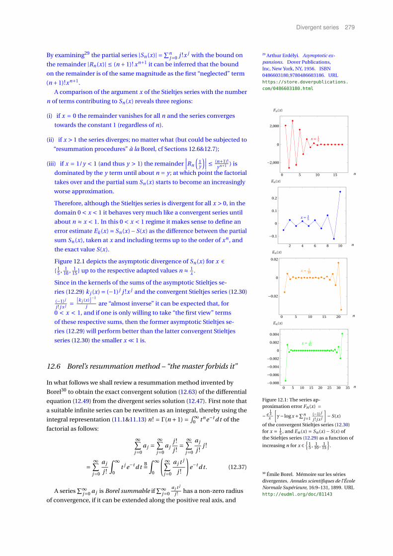
Divergent series 279

By examining29 the partial series |Sn(x)| = ∑nj=0 j !x j with the bound on 29 Arthur Erdélyi. Asymptotic ex-

pansions. Dover Publications,Inc, New York, NY, 1956. ISBN0486603180,9780486603186. URLhttps://store.doverpublications.

com/0486603180.html

the remainder |Rn(x)| ≤ (n +1)! xn+1 it can be inferred that the bound

on the remainder is of the same magnitude as the first “neglected” term

(n +1)!xn+1.

A comparison of the argument x of the Stieltjes series with the number

n of terms contributing to Sn(x) reveals three regions:

(i) if x = 0 the remainder vanishes for all n and the series converges

towards the constant 1 (regardless of n).

(ii) if x > 1 the series diverges; no matter what (but could be subjected to

“resummation procedures” à la Borel, cf Sections 12.6&12.7);

(iii) if x = 1/y < 1 (and thus y > 1) the remainder∣∣∣Rn

(1y

)∣∣∣ ≤ (n+1)!yn+1 ) is

dominated by the y term until about n = y ; at which point the factorial

takes over and the partial sum Sn(x) starts to become an increasingly

worse approximation.

Therefore, although the Stieltjes series is divergent for all x > 0, in the

domain 0 < x < 1 it behaves very much like a convergent series until

about n ≈ x < 1. In this 0 < x < 1 regime it makes sense to define an

error estimate Ek (x) = Sn(x)−S(x) as the difference between the partial

sum Sn(x), taken at x and including terms up to the order of xn , and

the exact value S(x).

Figure 12.1 depicts the asymptotic divergence of Sn(x) for x ∈ 1

5 , 110 , 1

15 up to the respective adapted values n ≈ 1x .

0 5 10 15

−2,000

0

2,000

x = 15

n

Fn(x)

2 4 6 8 10

−0.1

0

0.1

0.2

x = 15

n

En(x)

0 5 10 15 20

−0.02

0

0.02

x = 110

n

En(x)

0 5 10 15 20 25 30 35−0.008

−0.006

−0.004

−0.002

0

0.002

0.004

x = 115

n

En(x)

Figure 12.1: The series ap-proximation error Fn (x) =− e

1x

x

[γ− log x +∑n

j=1(−1) j

j ! j x j

]− S(x)

of the convergent Stieltjes series (12.30)for x = 1

5 , and En (x) = Sn (x)− S(x) ofthe Stieltjes series (12.29) as a function of

increasing n for x ∈

15 , 1

10 , 115

.

Since in the kernerls of the sums of the asymptotic Stieltjes se-

ries (12.29) k j (x) = (−1) j j !x j and the convergent Stieltjes series (12.30)

(−1) j

j ! j x j =[k j (x)

]−1

j are “almost inverse” it can be expected that, for

0 < x < 1, and if one is only willing to take “the first view” terms

of these respective sums, then the former asymptotic Stieltjes se-

ries (12.29) will perform better than the latter convergent Stieltjes

series (12.30) the smaller x ¿ 1 is.

12.6 Borel’s resummation method – “the master forbids it”

In what follows we shall review a resummation method invented by

Borel30 to obtain the exact convergent solution (12.63) of the differential

30 Émile Borel. Mémoire sur les sériesdivergentes. Annales scientifiques de l’ÉcoleNormale Supérieure, 16:9–131, 1899. URLhttp://eudml.org/doc/81143

equation (12.49) from the divergent series solution (12.47). First note that

a suitable infinite series can be rewritten as an integral, thereby using the

integral representation (11.1&11.13) n! = Γ(n +1) = ∫ ∞0 t ne−t d t of the

factorial as follows:

∞∑j=0

a j =∞∑

j=0a j

j !j !

=∞∑

j=0

a j

j !j !

=∞∑

j=0

a j

j !

∫ ∞

0t j e−t d t

B=∫ ∞

0

( ∞∑j=0

a j t j

j !

)e−t d t . (12.37)

A series∑∞

j=0 a j is Borel summable if∑∞

j=0a j t j

j ! has a non-zero radius

of convergence, if it can be extended along the positive real axis, and

280 Mathematical Methods of Theoretical Physics

if the integral (12.37) is convergent. This integral is called the Borel

sum of the series. It can be obtained by taking a j , computing the sum

σ(t) = ∑∞j=0

a j t j

j ! , and integrating σ(t) along the positive real axis with a

“weight factor” e−t .

More generally, suppose

S(z) = z∞∑

j=0a j z j =

∞∑j=0

a j z j+1 (12.38)

is some formal power series. Then its Borel transformation is defined by

∞∑j=0

a j z j+1 =∞∑

j=0a j z j+1 j !

j !=

∞∑j=0

a j z j+1

j !j !︸︷︷︸∫ ∞

0 t j e−t d t

=∞∑

j=0

a j z j

j !

∫ ∞

0t j e−t zd t

B=∫ ∞

0

( ∞∑j=0

a j (zt ) j

j !

)e−t zd t

[variable substitution y = zt , t = y

z, d y = z d t , d t = d y

z]

B=∫ ∞

0

( ∞∑j=0

a j y j

j !

)e−

yz d y =

∫ ∞

0BS(y)e−

yz d y . (12.39)

Often, this is written with z = 1/t , such that the Borel transformation is

defined by

∞∑j=0

a j t−( j+1) B=∫ ∞

0BS(y)e−y t d y . (12.40)

The Borel transform31 of S(z) =∑∞j=0 a j z j+1 =∑∞

j=0 a j t−( j+1) is thereby 31 This definition differs from the standarddefinition of the Borel transform basedon coefficients a j with S(z) = ∑∞

j=0 a j z j

introduced in Hagen Kleinert and VerenaSchulte-Frohlinde. Critical Proper-ties of φ4-Theories. World Scientific,Singapore, 2001. ISBN 9810246595,Mario Flory, Robert C. Helling, andConstantin Sluka. How I learned tostop worrying and love QFT, 2012. URLhttps://arxiv.org/abs/1201.2714.course presented by Robert C. Helling atthe Ludwig-Maximilians-UniversitätMünchen in the summer of 2011,notes by Mario Flory and ConstantinSluka, Daniele Dorigoni. An in-troduction to resurgence, trans-series and alien calculus, 2014. URLhttps://arxiv.org/abs/1411.3585

and Ovidiu Costin and Gerald VDunne. Introduction to resurgenceand non-perturbative physics, 2018.URL https://ethz.ch/content/

dam/ethz/special-interest/

phys/theoretical-physics/

computational-physics-dam/

alft2018/Dunne.pdf. slides of a talkat the ETH Zürich, March 7-9, 2018.

defined as

BS(y) =∞∑

j=0

a j y j

j !. (12.41)

In the following, a few examples will be given.

(i) The Borel sum of Grandi’s series (12.5) is equal to its Abel sum:

s =∞∑

j=0(−1) j B=

∫ ∞

0

( ∞∑j=0

(−1) j t j

j !

)e−t d t

=∫ ∞

0

( ∞∑j=0

(−t ) j

j !

)︸ ︷︷ ︸

e−t

e−t d t =∫ ∞

0e−2t d t

[variable substitution 2t = ζ,d t = 1

2dζ]

= 1

2

∫ ∞

0e−ζdζ

= 1

2

(−e−ζ

)∣∣∣∞ζ=0

= 1

2

−e−∞︸︷︷︸=0

+ e−0︸︷︷︸=1

= 1

2. (12.42)

Divergent series 281

(ii) A similar calculation for s2 defined in Equation (12.15) yields

s2 =∞∑

j=0(−1) j+1 j = (−1)

∞∑j=1

(−1) j jB=−

∫ ∞

0

( ∞∑j=1

(−1) j j t j

j !

)e−t d t

=−∫ ∞

0

( ∞∑j=1

(−t ) j

( j −1)!

)e−t d t =−

∫ ∞

0

( ∞∑j=0

(−t ) j+1

j !

)e−t d t

=−∫ ∞

0(−t )

( ∞∑j=0

(−t ) j

j !

)︸ ︷︷ ︸

e−t

e−t d t =−∫ ∞

0(−t )e−2t d t

[variable substitution 2t = ζ,d t = 1

2dζ]

= 1

4

∫ ∞

0ζe−ζdζ= 1

4Γ(2) = 1

41! = 1

4,

(12.43)

which is again equal to the Abel sum.

(iii) The Borel transform of a “geometric” series (12.12) g (z) =az

∑∞j=0 z j = a

∑∞j=0 z j+1 with constant coefficients a and 0 > z > 1

is “The idea that a function could be deter-mined by a divergent asymptotic series wasa foreign one to the nineteenth centurymind. Borel, then an unknown youngman, discovered that his summationmethod gave the “right” answer for manyclassical divergent series. He decided tomake a pilgrimage to Stockholm to seeMittag-Leffler, who was the recognizedlord of complex analysis. Mittag-Lefflerlistened politely to what Borel had tosay and then, placing his hand upon thecomplete works by Weierstrass, his teacher,he said in Latin, “The Master forbids it.”quoted as A tale of Mark Kac on page38 by Michael Reed and Barry Simon.Methods of Modern Mathematical PhysicsIV: Analysis of Operators, volume 4 ofMethods of Modern Mathematical PhysicsVolume. Academic Press, New York, 1978.ISBN 0125850042,9780125850049. URLhttps://www.elsevier.com/books/

iv-analysis-of-operators/reed/

978-0-08-057045-7.

Bg (y) = a∞∑

j=0

y j

j != ae y . (12.44)

The Borel transformation (12.39) of this geometric series is

g (z)B=

∫ ∞

0Bg (y)e−

yz d y =

∫ ∞

0ae y e−

yz d y = a

∫ ∞

0e−

y(1−z)z d y[

variable substitution x =−y1− z

z,d y =− z

1− zd x

]= −az

1− z

∫ −∞

0ex d x = az

1− z

∫ 0

−∞ex d x = a

z

1− z( e0︸︷︷︸

1

−e−∞︸︷︷︸0

) = az

1− z.

(12.45)

Likewise, the Borel transformation (12.40) of the geometric series

g (t−1) = a∑∞

j=0 t−( j+1) with constant a and t > 1 is

g (t−1)B=

∫ ∞

0Bg (y)e−y t d y =

∫ ∞

0ae y e−y t d y = a

∫ ∞

0e−y(t−1)d y[

variable substitution x =−y(t −1),d y =− 1

t −1d x

]= −a

t −1

∫ −∞

0ex d x = a

t −1

∫ 0

−∞ex d x = a

1

t −1( e0︸︷︷︸

1

−e−∞︸︷︷︸0

) = a

t −1.

(12.46)

12.7 Asymptotic series as solutions of differential equations

Already in 1760 Euler observed32 that what is today known as the Stieltjes

32 Leonhard Euler. De seriebus diver-gentibus. Novi Commentarii AcademiaeScientiarum Petropolitanae, 5:205–237,1760. URL http://eulerarchive.maa.

org/pages/E247.html. In Opera Omnia:Series 1, Volume 14, pp. 585–617. Availableon the Euler Archive as E247

series multiplied by x; namely the series

s(x) = x −x2 +2x3 −6x4 + . . . =∞∑

j=0(−1) j j !x j+1 = xS(x), (12.47)

282 Mathematical Methods of Theoretical Physics

when differentiated, satisfies

d

d xs(x) = x − s(x)

x2 , (12.48)

and thus in some way can be considered “a solution” of the differential

equation (x2 d

d x+1

)s(x) = x, or

(d

d x+ 1

x2

)s(x) = 1

x; (12.49)

resulting in a differential operator of the form Lx = dd x + 1

x2 .

This equation has an irregular singularity at x = 0 because the coef-

ficient of the zeroth derivative 1x2 has a pole of order 2, which is greater

than 1. Therefore, (12.49) is not of the Fuchsian type.

Nevertheless, the differential equation (12.49) can be solved in four

different ways:

(i) by the convergent series solution (12.50) based on the Stieltjes func-

tion (12.28), as pointed out earlier (thereby putting in question spec-

ulations that it needs to be asymptotic divergent series to cope with

irregular singularities beyond the Frobenius Ansatz);

(ii) by a proper (Borel) summation of Euler’s divergent series (12.47);

(iii) by direct integration of (12.49); and

(iv) by evaluating Euler’s (asymptotic) divergent series (12.47) based on

the Stieltjes series (12.30) to “optimal order,” and by comparing this

approximation to the exact solution (by taking the difference).

Solution by convergent series

The differential equation (12.49) has a convergent series solution which

is inspired by the convergent series (12.30) for the Stieltjes function

multiplied by x; that is,

s(x) = xS(x) = e1x Γ

(0,

1

x

)=−e

1x

[γ− log x +

∞∑n=1

(−1)n

n!nxn

](12.50)

That (12.50) is indeed a solution of (12.49) can be seen by direct insertion

and a rather lengthy calculation.

Solution by asymptotic divergent series

Without prior knowledge of s(x) in (12.47) an immediate way to

solve (12.49) is a quasi ad hoc series Ansatz similar to Frobenius’ method;

but allowing more general, and also diverging, series:

u(x) =∞∑

j=0a j x j . (12.51)

Divergent series 283

When inserted into (12.49) u(x) yields(x2 d

d x+1

)u(x) =

(x2 d

d x+1

) ∞∑j=0

a j x j = x

x2∞∑

j=0a j j x j−1 +

∞∑j=0

a j x j =∞∑

j=0a j j x j+1 +

∞∑j=0

a j x j = x

[index substitution in first sum i = j +1, j = i −1; then i → j

]∞∑

i=1ai−1(i −1)xi +

∞∑j=0

a j x j = a0 +∞∑

j=1

(a j−1( j −1)+a j

)x j = x

a0 +a1x +∞∑

j=2

(a j−1( j −1)+a j

)x j = x. (12.52)

Since polynomials of different degrees are linear independent, a compari-

son of coefficients appearing on the left hand side of (12.52) with x yields

a0 = 0, a1 = 1,

a j =−a j−1( j −1) =−(−1) j ( j −1)! = (−1) j−1( j −1)! for j ≥ 2. (12.53)

This yields the sum (12.47) enumerated by Euler:

u(x) = 0+x +∞∑

j=2(−1) j−1( j −1)!x j

= [ j → j +1] = x +∞∑

j=1(−1) j j !x j+1 =

∞∑j=0

(−1) j j !x j+1 = s(x). (12.54)

Just as the Stieltjes series, s(x) is divergent for all x 6= 0: for j ≥ 2

its coefficients a j = (−1) j−1( j − 1)! have been enumerated in (12.53).

D’Alembert’s criterion yields

limj→∞

∣∣∣∣ a j+1

a j

∣∣∣∣= limj→∞

∣∣∣∣ (−1) j j !(−1) j−1( j −1)!

∣∣∣∣= limj→∞

j > 1. (12.55)

Solution by Borel resummation of the asymptotic convergent series

In what follows the Borel summation will be used to formally sum up

the divergent series (12.47) enumerated by Euler. A comparison be-

tween (12.38) and (12.47) renders the coefficients

a j = (−1) j j !, (12.56)

which can be used to compute the Borel transform (12.41) of Euler’s

divergent series (12.47)

BS(y) =∞∑

j=0

a j y j

j !=

∞∑j=0

(−1) j j ! y j

j !=

∞∑j=0

(−y) j = 1

1+ y. (12.57)

resulting in the Borel transformation (12.39 ) of Euler’s divergent se-

ries (12.47)

s(x) =∞∑

j=0a j z j+1 B=

∫ ∞

0BS(y)e−

yx d y =

∫ ∞

0

e−yx

1+ yd y[

variable substitution t = y

x,d y = zd t

]=

∫ ∞

0

xe−t

1+xtd t . (12.58)

284 Mathematical Methods of Theoretical Physics

Notice33 that the Borel transform (12.57) “rescales” or “pushes” the 33 Christiane Rousseau. Divergent series:Past, present, future. Mathematical Reports– Comptes rendus mathématiques, 38(3):85–98, 2016. URL https://arxiv.org/

abs/1312.5712

divergence of the series (12.47) with zero radius of convergence towards

a “disk” or interval with finite radius of convergence and a singularity at

y =−1.

Solution by integration

An exact solution of (12.49) can also be found directly by quadrature; that

is, by direct integration (see, for instance, Chapter one of Ref.34). It is not

34 Garrett Birkhoff and Gian-Carlo Rota.Ordinary Differential Equations. JohnWiley & Sons, New York, Chichester,Brisbane, Toronto, fourth edition, 1959,1960, 1962, 1969, 1978, and 1989

immediately obvious how to utilize direct integration in this case; the

trick is to make the following Ansatz:

s(x) = y(x)exp

(−

∫d x

x2

)= y(x)exp

[−

(− 1

x+C

)]= k y(x)e

1x , (12.59)

with constant k = e−C , so that the ordinary differential equation (12.49)

transforms into (x2 d

d x+1

)s(x) =

(x2 d

d x+1

)y(x)exp

(−

∫d x

x2

)= x,

x2 d

d x

[y exp

(−

∫d x

x2

)]+ y exp

(−

∫d x

x2

)= x,

x2 exp

(−

∫d x

x2

)d y

d x+x2 y

(− 1

x2

)exp

(−

∫d x

x2

)+ y exp

(−

∫d x

x2

)= x,

x2 exp

(−

∫d x

x2

)d y

d x= x,

exp

(−

∫d x

x2

)d y

d x= 1

x,

d y

d x=

exp(∫ d x

x2

)x

,

y(x) =∫

1

xe

∫x

d tt2 d x.

(12.60)

More precisely, insertion into (12.59) yields, for some a 6= 0,

s(x) = e−∫ x

ad tt2 y(x) =−e−

∫ xa

d tt2

∫ x

0e

∫ ta

d ss2

(−1

t

)d t

= e−(− 1

t

)∣∣xa

∫ x

0e − 1

s

∣∣ta

(1

t

)d t

= e1x − 1

a

∫ x

0e−

1t + 1

a

(1

t

)d t

= e1x e−

1a + 1

a︸ ︷︷ ︸=e0=1

∫ x

0e−

1t

(1

t

)d t

= e1x

∫ x

0

e−1t

td t

=∫ x

0

e1x − 1

t

td t . (12.61)

With a change of the integration variable

z

x= 1

t− 1

x, and thus z = x

t−1, and t = x

1+ z,

d t

d z=− x

(1+ z)2 , and thus d t =− x

(1+ z)2 d z,

and thusd t

t=

− x(1+z)2

x1+z

d z =− d z

1+ z, (12.62)

Divergent series 285

the integral (12.61) can be rewritten into the same form as Equa-

tion (12.58):

s(x) =∫ 0

∞

(− e−

zx

1+ z

)d z =

∫ ∞

0

e−zx

1+ zd z. (12.63)

Note that, whereas the series solution diverges for all nonzero x, the

solutions by quadrature (12.63) and by the Borel summation (12.58) are

identical. They both converge and are well defined for all x ≥ 0.

Let us now estimate the absolute difference between sk (x) which

represents the partial sum of the Borel transform (12.57) in the Borel

transformation (12.58), with a j = (−1) j j ! from (12.56), “truncated after

the kth term” and the exact solution s(x); that is, let us consider

Rk (x)def=

∣∣∣s(x)− sk (x)∣∣∣= ∣∣∣∣∣

∫ ∞

0

e−zx

1+ zd z −

k∑j=0

(−1) j j !x j+1

∣∣∣∣∣ . (12.64)

For any x ≥ 0 this difference can be estimated35 by a bound from 35 Christiane Rousseau. Divergent series:Past, present, future. Mathematical Reports– Comptes rendus mathématiques, 38(3):85–98, 2016. URL https://arxiv.org/

abs/1312.5712

above

Rk (x) ≤ k!xk+1; (12.65)

that is, this difference between the exact solution s(x) and the diverging

partial sum sk (x) may become smaller than the first neglected term, and

all subsequent ones.

For a proof, observe that, since a partial geometric series is the sum of

all the numbers in a geometric progression up to a certain power; that is,

k∑j=0

r j = 1+ r + r 2 +·· ·+ r j +·· ·+ r k . (12.66)

By multiplying both sides with 1− r , the sum (12.66) can be rewritten as

(1− r )k∑

j=0r j = (1− r )(1+ r + r 2 +·· ·+ r j +·· ·+ r k )

= 1+ r + r 2 +·· ·+ r j +·· ·+ r k − r (1+ r + r 2 +·· ·+ r j +·· ·+ r k + r k )

= 1+ r + r 2 +·· ·+ r j +·· ·+ r k − (r + r 2 +·· ·+ r j +·· ·+ r k + r k+1)

= 1− r k+1,

(12.67)

and, since the middle terms all cancel out,

k∑j=0

r j = 1− r k+1

1− r, or

k−1∑j=0

r j = 1− r k

1− r= 1

1− r− r k

1− r. (12.68)

Thus, for r =−ζ, it is true that

1

1+ζ =k−1∑j=0

(−1) j ζ j + (−1)k ζk

1+ζ , (12.69)

and, therefore,

f (x) =∫ ∞

0

e−ζx

1+ζdζ

=∫ ∞

0e−

ζx

[k−1∑j=0

(−1) j ζ j + (−1)k ζk

1+ζ

]dζ

=k−1∑j=0

(−1) j∫ ∞

0ζ j e−

ζx dζ+ (−1)k

∫ ∞

0

ζk e−ζx

1+ζ dζ. (12.70)

286 Mathematical Methods of Theoretical Physics

Since [cf Equation (11.13)]

k! = Γ(k +1) =∫ ∞

0zk e−z d z, (12.71)

one obtains∫ ∞

0ζ j e−

ζx dζ with substitution: z = ζ

x,dζ= xd z

=∫ ∞

0x j+1z j e−z d z = x j+1

∫ ∞

0z j e−z d z = x j+1k!, (12.72)

and hence

f (x) =k−1∑j=0

(−1) j∫ ∞

0ζ j e−

ζx dζ+ (−1)k

∫ ∞

0

ζk e−ζx

1+ζ dζ

=k−1∑j=0

(−1) j x j+1k!+∫ ∞

0(−1)k ζ

k e−ζx

1+ζ dζ

= fk (x)+Rk (x), (12.73)

where fk (x) represents the partial sum of the power series, and Rk (x)

stands for the remainder, the difference between f (x) and fk (x). The

absolute of the remainder can be estimated by

Rk (x) =∫ ∞

0

ζk e−ζx

1+ζ dζ≤∫ ∞

0ζk e−

ζx dζ= k!xk+1. (12.74)

0 5 10 15 20 250.0000001

0.000001

0.00001

0.0001

0.001

0.01

0.1

1

x = 110

x = 115

x = 15

k

Rk (x)

Figure 12.2: The absolute error Rk (x) as afunction of increasing k for x ∈ 1

5 , 110 , 1

15 .

The functional form k!xk (times x) of the absolute error (12.64) sug-

gests that, for 0 < x < 1, there is an “optimal” value k ≈ 1x with respect to

convergence of the partial sums s(k) associated with Euler’s asymptotic

expansion of the solution (12.47): up to this k-value the factor xk dom-

inates the estimated absolute rest (12.65) by suppressing it more than

k! grows. However, this suppression of the absolute error as k grows is

eventually – that is, if k > 1x – compensated by the factorial function, as

depicted in Figure 12.2: from k ≈ 1x the absolute error grows again, so

that the overall behavior of the absolute error Rk (x) as a function of k (at

constant x) is “bathtub”-shaped; with a “sink” or minimum at k ≈ 1x .

12.8 Divergence of perturbation series in quantum field the-

ory

A formal entity such as the solution of an ordinary differential equation

may have very different representations and encodings; some of them

with problematic issues. The means available are often not a matter of

choice but of pragmatism and even desperation.36 36 John P. Boyd. The devil’s invention:Asymptotic, superasymptotic andhyperasymptotic series. Acta ApplicandaeMathematica, 56:1–98, 1999. ISSN 0167-8019. D O I : 10.1023/A:1006145903624.URL https://doi.org/10.1023/A:

1006145903624

This seems to apply also to field theories: often one is restricted to

perturbative solutions in terms of power series. But these methods are

problematic as they are applied in a situation where they are forbidden.

Presently there are two known reasons for the occurrence of asymp-

totically divergent power series in perturbative quantum field theories:

one is associated with expansion at an essential singularity, such as z = 0

for the function e1z and the other with an exchange of the order of two

limits, such as exchanging an infinite sum with an integral if the domain

of integration is not compact.

Divergent series 287

12.8.1 Expansion at an essential singularity

The following argument is due to Dyson.37 Suppose the overall energy 37 Freeman J. Dyson. Divergenceof perturbation theory in quantumelectrodynamics. Physical Review,85(4):631–632, Feb 1952. D O I :10.1103/PhysRev.85.631. URL https:

//doi.org/10.1103/PhysRev.85.631;and J. C. Le Guillou and Jean Zinn-Justin.Large-Order Behaviour of PerturbationTheory, volume 7 of Current Physics-Sources and Comments. North Holland,Elsevier, Amsterdam, 1990,2013. ISBN9780444596208,0444885943,0444885978.URL https://www.

elsevier.com/books/

large-order-behaviour-of-perturbation-theory/

le-guillou/978-0-444-88597-5

of a system of a large number N À 1 of particles of charge q with mean

kinetic energy (aka “temperature”) T and mean absolute potential V

consists of a kinetic and a potential part, like

E ∼ T N +q2VN (N −1)

2≈ T N + q2V

2N 2, (12.75)

where N (N −1)/2 is the number of particle pairs. Then the ground state

energy is bound from below as long as the interaction is repulsive: that is,

q2 > 0. However, for an attractive effective interaction q2 < 0 and, in par-

ticular, in the presence of (electron-positron) pair creation, the ground

state may no longer be stable. As a result of this instability of the ground

state “around” q2 = 0 one must expect that any physical quantity F (q2)

which is calculated as a formal power series in the coupling constant

q2 cannot be analytic around q2 = 0. Because, intuitively, even if F (q2)

appears to be “well behaved” F (−q2) is not if the theory is unstable for

transitions from a repulsive to an attractive potential regime.

Therefore, it is strictly disallowed to develop F (q2) at q2 = 0 into a

Taylor series. Insistence (or ignorance) in doing what is forbidden is

penalized by an asymptotic divergent series at best.

To obtain a quantitative feeling for what is going on in such cases

consider38, the functional integral with a redefined exponential kernel 38 Thomas Sommer. Asymptotische Reihen,2019a. unpublished manuscriptfrom Equation (12.75): let N = x2, T =−α, and g =− q2V

2 , and

f(α, g

)= ∫ ∞

0e−αx2−g x4

d x. (12.76)

For negative g < 0 the term e−g x4 = e |g |x4

dominates the kernel, and

the integral (12.76) diverges. For α > 0 und g > 0 this integral has a

nonperturbative representation as

f(α, g

)= 1

4

√α

geα28g K 1

4

(α2

8g

), (12.77)

where Kν (x) is the modified Bessel funktion of the second kind (e.g., §9.6,

pp. 374-377 of Abramowitz and Stegun). http://mathworld.wolfram.com/

ModifiedBesselFunctionoftheSecondKind.

htmlA divergent series is obtained by expanding f

(α, g

)from (12.76) in a

Taylor series of the “coupling constant” g 6= 0 at g = 0; and, in particular,

by taking the limit n →∞ of the partial sum up to order n of g :

fn(α, g

)= 1

2

n∑k=0

(−1)k

k!Γ

(2k + 1

2

)α2k+ 1

2

g k

= 1

2

[pπ+

n∑k=1

(−1)k

k!Γ

(2k + 1

2

)α2k+ 1

2

g k

]

= 1

2p

a

(− g

a2

)n Γ( 1

2 (4n +1))

Γ(n +1)2F2

(1,−n;

1

4−n,

3

4−n;

a2

4g

). (12.78)

For fixed α = 1 the asymptotic divergence of (12.78) for n → ∞manifests itself differently for different values of g > 0:

• For g = 1 the nonperturbative expression (12.77) yields

f (1,1) =∫ ∞

0e−x2−x4

d x = 1

4e

18 K 1

4

(1

8

)≈ 0.684213, (12.79)

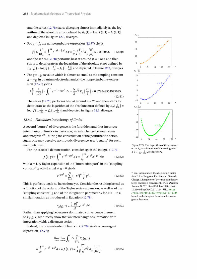
288 Mathematical Methods of Theoretical Physics

and the series (12.78) starts diverging almost immediately as the log-

arithm of the absolute error defined by Rn(1) = log∣∣ f (1,1)− fn (1,1)

∣∣and depicted in Figure 12.3, diverges.

0 5 10 15 20

0

20

40

60

q = 1

n

Rn(1)

0 5 10 15 20

−5

0

5

10

15

20

q = 110

n

Rn( 1

10

)

0 20 40 60 80−30

−20

−10

0

q = 1100

n

Rn( 1

100

)

Figure 12.3: The logarithm of the absoluteerror Rn as a function of increasing n forq ∈ 1, 1

10 , 1100 , respectively.

• For g = 110 the nonperturbative expression (12.77) yields

f

(1,

1

10

)=

∫ ∞

0e−x2− 1

10 x4d x = 1

2

√5

2e

54 K 1

4

(5

4

)≈ 0.837043, (12.80)

and the series (12.78) performs best at around n = 3 or 4 and then

starts to deteriorate as the logarithm of the absolute error defined by

Rn( 1

10

)= log∣∣ f

(1, 1

10

)− fn(1, 1

10

)∣∣ and depicted in Figure 12.3, diverges.

• For g = 1100 (a value which is almost as small as the coupling constant

g = 1137 in quantum electrodynamics) the nonperturbative expres-

sion (12.77) yields

f

(1,

1

100

)=

∫ ∞

0e−x2− 1

100 x4d x = 5

2e

252 K 1

4

(25

2

)≈ 0.879849554945695.

(12.81)

The series (12.78) performs best at around n = 25 and then starts to

deteriorate as the logarithm of the absolute error defined by Rn( 1

100

)=log

∣∣ f(1, 1

100

)− fn(1, 1

100

)∣∣ and depicted in Figure 12.3, diverges.

12.8.2 Forbidden interchange of limits

A second “source” of divergence is the forbidden and thus incorrect

interchange of limits – in particular, an interchange between sums

and integrals 39 – during the construction of the perturbation series.

39 See, for instance, the discussion in Sec-tion II.A of Sergio A. Pernice and GerardoOleaga. Divergence of perturbation theory:Steps towards a convergent series. PhysicalReview D, 57:1144–1158, Jan 1998. D O I :10.1103/PhysRevD.57.1144. URL https:

//doi.org/10.1103/PhysRevD.57.1144

based on Lebesgue’s dominated conver-gence theorem.

Again one may perceive asymptotic divergence as a “penalty” for such

manipulations.

For the sake of a demonstration, consider again the integral (12.76)

f(1, g

)= ∫ ∞

0e−x2−g x4

d x =∫ ∞

0e−x2

e−g x4d x (12.82)

with α= 1. A Taylor expansion of the “interaction part” in the “coupling

constant” g of its kernel at g = 0 yields

e−g x4 =∞∑

k=0

(−x4)n 1

k!g k . (12.83)

This is perfectly legal; no harm done yet. Consider the resulting kernel as

a function of the order k of the Taylor series expansion, as well as of the

“coupling constant” g and of the integration parameter x for α = 1 in a

similar notation as introduced in Equation (12.78):

Fk (g , x) =(−g

)k

k!e−x2

x4k . (12.84)

Rather than applying Lebesgue’s dominated convergence theorem

to Fk (g , x) we directly show that an interchange of summation with

integration yields a divergent series.

Indeed, the original order of limits in (12.76) yields a convergent

expression (12.77):

limt→∞ lim

n→∞

∫ t

0d x

n∑k=0

Fk (g , x)

=∫ ∞

0e−x2−g x4

d x = f(1, g

)= 1

4

√1

ge

18g K 1

4

(1

8g

). (12.85)

Divergent series 289

However, for g 6= 0 the interchange of limits results in a divergent

series:

limn→∞ lim

t→∞

n∑i=0

∫ t

0Fn(1, g , x)d x = lim

n→∞ fn(1, g

)= lim

n→∞1

2

n∑i=0

(−g )k

k!Γ

(2k + 1

2

)= 1

2

[pπ+ lim

n→∞n∑

i=1

(−g )k

k!Γ

(2k + 1

2

)].

(12.86)

Notice that both the direct Taylor expansion of f (α, g ) at the singular

point z = 0 as well as the interchange of the summation from the legal

Taylor expansion of e−g x4with the integration in (12.85) yield the same

(asymptotic) divergent expressions (12.78) and (12.86).

12.8.3 On the usefulness of asymptotic expansions in quantum

field theory

It may come as a surprise that calculations involving asymptotic expan-

sions in the coupling constants yield perturbation series which perform

well for many empirical predictions – in some cases40 the differences

40 K. Hagiwara, A. D. Martin, DaisukeNomura, and T. Teubner. Improvedpredictions for g −2 of the muon andαQED

(m2

z). Physics Letters B, 649(2):

173–179, 2007. ISSN 0370-2693. D O I :10.1016/j.physletb.2007.04.012. URLhttps://doi.org/10.1016/j.physletb.

2007.04.012

between experiment and prediction as small as 10−9. Depending on the

temperament and personal inclinations to accept results from “wrong”

evaluations this may be perceived optimistically as well as pessimisti-

cally.

As we have seen the quality of such asymptotic expansions depends

on the magnitude of the expansion parameter: the higher it gets the

worse is the quality of prediction in larger orders. And the approximation

will never be able to reach absolute accuracy. However in regimes such

as quantum electrodynamics, for which the expansion parameter is of

the order of 100, for all practical purposes41 and relative to our limited

41 John Stuard Bell. Against ‘measurement’.Physics World, 3:33–41, 1990. D O I :10.1088/2058-7058/3/8/26. URL https:

//doi.org/10.1088/2058-7058/3/8/26

means to compute the high order terms, such an asymptotic divergent

perturbative expansion might be “good enough” anyway. But what if this

parameter is of the order of 1?

Another question is whether resummation procedures can “recover”

the “right” solution in terms of analytic functions. This is an ongoing

field of research. As long as low-dimensional toy models such as the one

covered in earlier sections are studied this might be possible, say, by (vari-

ants) of Borel summations.42 However, for realistic, four-dimensional

42 David Sauzin. Introduction to 1-summability and resurgence, 2014. URLhttps://arxiv.org/abs/1405.0356;and Ramon Miravitllas Mas. Resurgence,a problem of missing exponentialcorrections in asymptotic expansions,2019. URL https://arxiv.org/abs/

1904.07217

field theoretic models the situation may be very different and “much

harder.”43 Let me finally quote Arthur M. Jaffe and Edward Witten:44

43 Jean Zinn-Justin. Summation ofdivergent series: Order-dependentmapping. Applied Numerical Mathematics,60(12):1454–1464, 2010. ISSN 0168-9274.D O I : 10.1016/j.apnum.2010.04.002. URLhttps://doi.org/10.1016/j.apnum.

2010.04.002; and Arnold Neumaier,2019. URL https://www.mat.univie.

ac.at/~neum/physfaq/topics/summing.accessed on October 28th, 2019

44 Arthur M. Jaffe and Edward Witten.Quantum Yang-Mills theory, 2000. URLhttps://www.claymath.org/sites/

default/files/yangmills.pdf. ClayMathematics Institute Millenium Prizeproblem

“In most known examples, perturbation series, i.e., power series in the

coupling constant, are divergent expansions; even Borel and other resum-

mation methods have limited applicability.”

c

Bibliography 291

Bibliography

Alastair A. Abbott, Cristian S. Calude, and Karl Svozil. A variant of the

Kochen-Specker theorem localising value indefiniteness. Journal of

Mathematical Physics, 56(10):102201, 2015. D O I : 10.1063/1.4931658.

URL https://doi.org/10.1063/1.4931658.

Milton Abramowitz and Irene A. Stegun, editors. Handbook of Mathe-

matical Functions with Formulas, Graphs, and Mathematical Tables.

Number 55 in National Bureau of Standards Applied Mathematics

Series. U.S. Government Printing Office, Washington, D.C., 1964. URL

http://www.math.sfu.ca/~cbm/aands/.

Lars V. Ahlfors. Complex Analysis: An Introduction of the Theory of Analytic

Functions of One Complex Variable. McGraw-Hill Book Co., New York,

third edition, 1978.

Martin Aigner and Günter M. Ziegler. Proofs from THE BOOK. Springer,

Heidelberg, four edition, 1998-2010. ISBN 978-3-642-00856-6,978-3-642-

00855-9. D O I : 10.1007/978-3-642-00856-6. URL https://doi.org/10.

1007/978-3-642-00856-6.

M. A. Al-Gwaiz. Sturm-Liouville Theory and its Applications. Springer,

London, 2008.

A. D. Alexandrov. On Lorentz transformations. Uspehi Mat. Nauk., 5(3):187,

1950.

A. D. Alexandrov. A contribution to chronogeometry. Canadian Journal of

Math., 19:1119–1128, 1967.

A. D. Alexandrov. Mappings of spaces with families of cones and space-

time transformations. Annali di Matematica Pura ed Applicata, 103:

229–257, 1975. ISSN 0373-3114. D O I : 10.1007/BF02414157. URL

https://doi.org/10.1007/BF02414157.

A. D. Alexandrov. On the principles of relativity theory. In Classics of

Soviet Mathematics. Volume 4. A. D. Alexandrov. Selected Works, pages

289–318. 1996.

George E. Andrews, Richard Askey, and Ranjan Roy. Special Functions, vol-

ume 71 of Encyclopedia of Mathematics and its Applications. Cambridge

University Press, Cambridge, 1999. ISBN 0-521-62321-9.

292 Mathematical Methods of Theoretical Physics

Tom M. Apostol. Mathematical Analysis: A Modern Approach to Advanced

Calculus. Addison-Wesley Series in Mathematics. Addison-Wesley,

Reading, MA, second edition, 1974. ISBN 0-201-00288-4.

Thomas Aquinas. Summa Theologica. Translated by Fathers of the English

Dominican Province. Christian Classics Ethereal Library, Grand Rapids,

MI, 1981. URL http://www.ccel.org/ccel/aquinas/summa.html.

George B. Arfken and Hans J. Weber. Mathematical Methods for Physicists.

Elsevier, Oxford, sixth edition, 2005. ISBN 0-12-059876-0;0-12-088584-0.

Shiri Artstein-Avidan and Boaz A. Slomka. The fundamental theo-

rems of affine and projective geometry revisited. Communica-

tions in Contemporary Mathematics, 19(05):1650059, 2016. D O I :

10.1142/S0219199716500590. URL https://doi.org/10.1142/

S0219199716500590.

Sheldon Axler, Paul Bourdon, and Wade Ramey. Harmonic Function

Theory, volume 137 of Graduate texts in mathematics. second edition,

1994. ISBN 0-387-97875-5.

L. E. Ballentine. Quantum Mechanics. Prentice Hall, Englewood Cliffs, NJ,

1989.

Werner Balser. From Divergent Power Series to Analytic Functions: Theory

and Application of Multisummable Power Series, volume 1582 of

Lecture Notes in Mathematics. Springer-Verlag Berlin Heidelberg, Berlin,

Heidelberg, 1994. ISBN 978-3-540-48594-0,978-3-540-58268-7. D O I :

10.1007/BFb0073564. URL https://doi.org/10.1007/BFb0073564.

Asim O. Barut. e = ×ω. Physics Letters A, 143(8):349–352, 1990. ISSN

0375-9601. D O I : 10.1016/0375-9601(90)90369-Y. URL https://doi.

org/10.1016/0375-9601(90)90369-Y.

John Stuard Bell. Against ‘measurement’. Physics World, 3:33–41, 1990.

D O I : 10.1088/2058-7058/3/8/26. URL https://doi.org/10.1088/

2058-7058/3/8/26.

W. W. Bell. Special Functions for Scientists and Engineers. D. Van Nostrand

Company Ltd, London, 1968.

Carl M. Bender and Steven A. Orszag. Andvanced Mathematical Methods

for Scientists and Enineers I. Asymptotic Methods and Perturbation

Theory. International Series in Pure and Applied Mathematics. McGraw-

Hill and Springer-Verlag, New York, NY, 1978,1999. ISBN 978-1-4757-

3069-2,978-0-387-98931-0,978-1-4419-3187-0. D O I : 10.1007/978-1-

4757-3069-2. URL https://doi.org/10.1007/978-1-4757-3069-2.

Walter Benz. Geometrische Transformationen. BI Wissenschaftsverlag,

Mannheim, 1992.

George Berkeley. A Treatise Concerning the Principles of Human Knowledge.

1710. URL http://www.gutenberg.org/etext/4723.

Bibliography 293

Michael Berry. Asymptotics, superasymptotics, hyperasymptotics . . .. In

Harvey Segur, Saleh Tanveer, and Herbert Levine, editors, Asymptotics

beyond All Orders, volume 284 of NATO ASI Series, pages 1–14. Springer,

1992. ISBN 978-1-4757-0437-2. D O I : 10.1007/978-1-4757-0435-8. URL

https://doi.org/10.1007/978-1-4757-0435-8.

Garrett Birkhoff and Gian-Carlo Rota. Ordinary Differential Equations.

John Wiley & Sons, New York, Chichester, Brisbane, Toronto, fourth

edition, 1959, 1960, 1962, 1969, 1978, and 1989.

Garrett Birkhoff and John von Neumann. The logic of quantum mechanics.

Annals of Mathematics, 37(4):823–843, 1936. D O I : 10.2307/1968621.

URL https://doi.org/10.2307/1968621.

Norman Bleistein and Richard A. Handelsman. Asymptotic Expansions

of Integrals. Dover Books on Mathematics. Dover, 1975, 1986. ISBN

0486650820,9780486650821.

Guy Bonneau, Jacques Faraut, and Galliano Valent. Self-adjoint extensions

of operators and the teaching of quantum mechanics. American

Journal of Physics, 69(3):322–331, 2001. D O I : 10.1119/1.1328351. URL

https://doi.org/10.1119/1.1328351.

H. J. Borchers and G. C. Hegerfeldt. The structure of space-time transfor-

mations. Communications in Mathematical Physics, 28(3):259–266, 1972.

URL http://projecteuclid.org/euclid.cmp/1103858408.

Émile Borel. Mémoire sur les séries divergentes. Annales scientifiques de

l’École Normale Supérieure, 16:9–131, 1899. URL http://eudml.org/

doc/81143.

John P. Boyd. The devil’s invention: Asymptotic, superasymptotic

and hyperasymptotic series. Acta Applicandae Mathematica, 56:

1–98, 1999. ISSN 0167-8019. D O I : 10.1023/A:1006145903624. URL

https://doi.org/10.1023/A:1006145903624.

Percy W. Bridgman. A physicist’s second reaction to Mengenlehre. Scripta

Mathematica, 2:101–117, 224–234, 1934.

Yuri Alexandrovich Brychkov and Anatolii Platonovich Prudnikov. Hand-

book of special functions: derivatives, integrals, series and other for-

mulas. CRC/Chapman & Hall Press, Boca Raton, London, New York,

2008.

B.L. Burrows and D.J. Colwell. The Fourier transform of the unit step

function. International Journal of Mathematical Education in Science

and Technology, 21(4):629–635, 1990. D O I : 10.1080/0020739900210418.

URL https://doi.org/10.1080/0020739900210418.

Adán Cabello. Experimentally testable state-independent quantum

contextuality. Physical Review Letters, 101(21):210401, 2008. D O I :

10.1103/PhysRevLett.101.210401. URL https://doi.org/10.1103/

PhysRevLett.101.210401.

294 Mathematical Methods of Theoretical Physics

Adán Cabello, José M. Estebaranz, and G. García-Alcaine. Bell-Kochen-

Specker theorem: A proof with 18 vectors. Physics Letters A, 212(4):

183–187, 1996. D O I : 10.1016/0375-9601(96)00134-X. URL https:

//doi.org/10.1016/0375-9601(96)00134-X.

Cristian S. Calude and Karl Svozil. Spurious, emergent laws in num-

ber worlds. Philosophies, 4(2):17, 2019. ISSN 2409-9287. D O I :

10.3390/philosophies4020017. URL https://doi.org/10.3390/

philosophies4020017.

Albert Camus. Le Mythe de Sisyphe (English translation: The Myth of

Sisyphus). 1942.

Bernard Candelpergher. Ramanujan Summation of Divergent Series,

volume 2185 of Lecture Notes in Mathematics. Springer International

Publishing, Cham, Switzerland, 2017. ISBN 978-3-319-63630-6,978-3-

319-63629-0. D O I : 10.1007/978-3-319-63630-6. URL https://doi.

org/10.1007/978-3-319-63630-6.

Rudolf Carnap. The elimination of metaphysics through logical analysis

of language. In Alfred Jules Ayer, editor, Logical Positivism, pages 60–81.

Free Press, New York, 1959. translated by Arthur Arp.

Yonah Cherniavsky. A note on separation of variables. International

Journal of Mathematical Education in Science and Technology, 42(1):

129–131, 2011. D O I : 10.1080/0020739X.2010.519793. URL https:

//doi.org/10.1080/0020739X.2010.519793.

Tai L. Chow. Mathematical Methods for Physicists: A Concise Introduction.

Cambridge University Press, Cambridge, 2000. ISBN 9780511755781.

D O I : 10.1017/CBO9780511755781. URL https://doi.org/10.1017/

CBO9780511755781.

J. B. Conway. Functions of Complex Variables. Volume I. Springer, New

York, 1973.

Sergio Ferreira Cortizo. On Dirac’s delta calculus, 1995. URL https:

//arxiv.org/abs/funct-an/9510004.

Ovidiu Costin. Asymptotics and Borel Summability, volume 141

of Monographs and surveys in pure and applied mathematics.

Chapman & Hall/CRC, Taylor & Francis Group, Boca Raton, FL,

2009. ISBN 9781420070316. URL https://www.crcpress.

com/Asymptotics-and-Borel-Summability/Costin/p/book/

9781420070316.

Ovidiu Costin and Gerald V Dunne. Introduction to resurgence and

non-perturbative physics, 2018. URL https://ethz.ch/content/

dam/ethz/special-interest/phys/theoretical-physics/

computational-physics-dam/alft2018/Dunne.pdf. slides of a

talk at the ETH Zürich, March 7-9, 2018.

Rene Descartes. Discours de la méthode pour bien conduire sa raison

et chercher la verité dans les sciences (Discourse on the Method of

Bibliography 295

Rightly Conducting One’s Reason and of Seeking Truth). 1637. URL

http://www.gutenberg.org/etext/59.

Rene Descartes. The Philosophical Writings of Descartes. Volume 1.

Cambridge University Press, Cambridge, 1985. translated by John

Cottingham, Robert Stoothoff and Dugald Murdoch.

Florin Diacu. The solution of the n-body problem. The Mathematical

Intelligencer, 18:66–70, SUM 1996. D O I : 10.1007/bf03024313. URL

https://doi.org/10.1007/bf03024313.

Hermann Diels and Walther Kranz. Die Fragmente der Vorsokratiker.

Weidmannsche Buchhandlung, Berlin, sixth edition, 1906,1952. ISBN

329612201X,9783296122014. URL https://biblio.wiki/wiki/Die_

Fragmente_der_Vorsokratiker.

Robert Balson Dingle. Asymptotic expansions: their derivation and

interpretation. Academic Press, London, 1973. URL https:

//michaelberryphysics.files.wordpress.com/2013/07/dingle.

pdf.

Paul Adrien Maurice Dirac. The Principles of Quantum Mechanics.

Oxford University Press, Oxford, fourth edition, 1930, 1958. ISBN

9780198520115.

Hans Jörg Dirschmid. Tensoren und Felder. Springer, Vienna, 1996.

Daniele Dorigoni. An introduction to resurgence, trans-series and alien

calculus, 2014. URL https://arxiv.org/abs/1411.3585.

Dean G. Duffy. Green’s Functions with Applications. Chapman and

Hall/CRC, Boca Raton, 2001.

Thomas Durt, Berthold-Georg Englert, Ingemar Bengtsson, and Karol Zy-

czkowski. On mutually unbiased bases. International Journal of Quan-

tum Information, 8:535–640, 2010. D O I : 10.1142/S0219749910006502.

URL https://doi.org/10.1142/S0219749910006502.

Anatolij Dvurecenskij. Gleason’s Theorem and Its Applications, volume 60

of Mathematics and its Applications. Kluwer Academic Publishers,

Springer, Dordrecht, 1993. ISBN 9048142091,978-90-481-4209-5,978-94-

015-8222-3. D O I : 10.1007/978-94-015-8222-3. URL https://doi.org/

10.1007/978-94-015-8222-3.

Freeman J. Dyson. Divergence of perturbation theory in quantum

electrodynamics. Physical Review, 85(4):631–632, Feb 1952. D O I :

10.1103/PhysRev.85.631. URL https://doi.org/10.1103/PhysRev.

85.631.

Heinz-Dieter Ebbinghaus, Hans Hermes, Friedrich Hirzebruch, Max

Koecher, Klaus Mainzer, Jürgen Neukirch, Alexander Prestel, and

Reinhold Remmert. Numbers, volume 123 of Readings in Mathematics.

Springer-Verlag New York, New York, NY, 1991. ISBN 978-1-4612-1005-4.

D O I : 10.1007/978-1-4612-1005-4. URL https://doi.org/10.1007/

978-1-4612-1005-4. Translated by H. L. S. Orde.

296 Mathematical Methods of Theoretical Physics

Charles Henry Edwards Jr. The Historical Development of the Calculus.

Springer-Verlag, New York, 1979. ISBN 978-1-4612-6230-5. D O I :

10.1007/978-1-4612-6230-5. URL https://doi.org/10.1007/

978-1-4612-6230-5.

Artur Ekert and Peter L. Knight. Entangled quantum systems and the

Schmidt decomposition. American Journal of Physics, 63(5):415–423,

1995. D O I : 10.1119/1.17904. URL https://doi.org/10.1119/1.

17904.

John Eliott. Group theory, 2015. URL https://youtu.be/O4plQ5ppg9c?

list=PLAvgI3H-gclb_Xy7eTIXkkKt3KlV6gk9_. accessed on March

12th, 2018.

Arthur Erdélyi. Asymptotic expansions. Dover Publications, Inc, New

York, NY, 1956. ISBN 0486603180,9780486603186. URL https://store.

doverpublications.com/0486603180.html.

Leonhard Euler. De seriebus divergentibus. Novi Commentarii

Academiae Scientiarum Petropolitanae, 5:205–237, 1760. URL

http://eulerarchive.maa.org/pages/E247.html. In Opera Omnia:

Series 1, Volume 14, pp. 585–617. Available on the Euler Archive as

E247.

Lawrence C. Evans. Partial differential equations, volume 19 of Graduate

Studies in Mathematics. American Mathematical Society, Providence,

Rhode Island, 1998.

Graham Everest, Alf van der Poorten, Igor Shparlinski, and Thomas Ward.

Recurrence sequences. Volume 104 in the AMS Surveys and Monographs

series. American mathematical Society, Providence, RI, 2003.

Hugh Everett III. In Jeffrey A. Barrett and Peter Byrne, editors, The Everett

Interpretation of Quantum Mechanics: Collected Works 1955-1980 with

Commentary. Princeton University Press, Princeton, NJ, 2012. ISBN

9780691145075. URL http://press.princeton.edu/titles/9770.

html.

William Norrie Everitt. A catalogue of Sturm-Liouville differential

equations. In Werner O. Amrein, Andreas M. Hinz, and David B. Pearson,

editors, Sturm-Liouville Theory, Past and Present, pages 271–331.

Birkhäuser Verlag, Basel, 2005. URL http://www.math.niu.edu/SL2/

papers/birk0.pdf.

Franz Serafin Exner. Über Gesetze in Naturwissenschaft und Human-

istik: Inaugurationsrede gehalten am 15. Oktober 1908. Hölder,

Ebooks on Demand Universitätsbibliothek Wien, Vienna, 1909,

2016. URL http://phaidra.univie.ac.at/o:451413. han-

dle https://hdl.handle.net/11353/10.451413, o:451413, Uploaded:

30.08.2016.

Richard Phillips Feynman. The Feynman lectures on computation. Addison-

Wesley Publishing Company, Reading, MA, 1996. edited by A.J.G. Hey

and R. W. Allen.

Bibliography 297

Stefan Filipp and Karl Svozil. Generalizing Tsirelson’s bound on Bell

inequalities using a min-max principle. Physical Review Letters, 93:

130407, 2004. D O I : 10.1103/PhysRevLett.93.130407. URL https:

//doi.org/10.1103/PhysRevLett.93.130407.

Mario Flory, Robert C. Helling, and Constantin Sluka. How I learned to

stop worrying and love QFT, 2012. URL https://arxiv.org/abs/

1201.2714. course presented by Robert C. Helling at the Ludwig-

Maximilians-Universität München in the summer of 2011, notes by

Mario Flory and Constantin Sluka.

Philipp Frank. Das Kausalgesetz und seine Grenzen. Springer, Vienna, 1932.

Philipp Frank and R. S. Cohen (Editor). The Law of Causality and its Limits

(Vienna Circle Collection). Springer, Vienna, 1997. ISBN 0792345517.

D O I : 10.1007/978-94-011-5516-8. URL https://doi.org/10.1007/

978-94-011-5516-8.

Eberhard Freitag and Rolf Busam. Funktionentheorie 1. Springer, Berlin,

Heidelberg, fourth edition, 1993,1995,2000,2006.

Eberhard Freitag and Rolf Busam. Complex Analysis. Springer, Berlin,

Heidelberg, 2005.

Sigmund Freud. Ratschläge für den Arzt bei der psychoanalytischen Be-

handlung. In Anna Freud, E. Bibring, W. Hoffer, E. Kris, and O. Isakower,

editors, Gesammelte Werke. Chronologisch geordnet. Achter Band.

Werke aus den Jahren 1909–1913, pages 376–387. Fischer, Frankfurt

am Main, 1912, 1999. URL http://gutenberg.spiegel.de/buch/

kleine-schriften-ii-7122/15.

Theodore W. Gamelin. Complex Analysis. Springer, New York, 2001.

Elisabeth Garber, Stephen G. Brush, and C. W. Francis Everitt. Maxwell

on Heat and Statistical Mechanics: On “Avoiding All Personal Enquiries”

of Molecules. Associated University Press, Cranbury, NJ, 1995. ISBN

0934223343.

I. M. Gel’fand and G. E. Shilov. Generalized Functions. Vol. 1: Properties

and Operations. Academic Press, New York, 1964. Translated from the

Russian by Eugene Saletan.

François Gieres. Mathematical surprises and Dirac’s formalism in

quantum mechanics. Reports on Progress in Physics, 63(12):1893–1931,

2000. D O I : https://doi.org/10.1088/0034-4885/63/12/201. URL

10.1088/0034-4885/63/12/201.

Andrew M. Gleason. Measures on the closed subspaces of a Hilbert

space. Journal of Mathematics and Mechanics (now Indiana University

Mathematics Journal), 6(4):885–893, 1957. ISSN 0022-2518. D O I :

10.1512/iumj.1957.6.56050. URL https://doi.org/10.1512/iumj.

1957.6.56050.

298 Mathematical Methods of Theoretical Physics

Ian Goodfellow, Yoshua Bengio, and Aaron Courville. Deep Learning.

MIT Press, Cambridge, MA, November 2016. ISBN 9780262035613,

9780262337434. URL https://mitpress.mit.edu/books/

deep-learning.

I. S. Gradshteyn and I. M. Ryzhik. Tables of Integrals, Series, and Products,

6th ed. Academic Press, San Diego, CA, 2000.

Dietrich Grau. Übungsaufgaben zur Quantentheorie. Karl Thiemig, Karl

Hanser, München, 1975, 1993, 2005. URL http://www.dietrich-grau.

at.

Richard J. Greechie. Orthomodular lattices admitting no states. Journal of

Combinatorial Theory. Series A, 10:119–132, 1971. D O I : 10.1016/0097-

3165(71)90015-X. URL https://doi.org/10.1016/0097-3165(71)

90015-X.

Robert E. Greene and Stephen G. Krantz. Function theory of one complex

variable, volume 40 of Graduate Studies in Mathematics. American

Mathematical Society, Providence, Rhode Island, third edition, 2006.

Werner Greub. Linear Algebra, volume 23 of Graduate Texts in Mathemat-

ics. Springer, New York, Heidelberg, fourth edition, 1975.

K. W. Gruenberg and A. J. Weir. Linear Geometry, volume 49 of Grad-

uate Texts in Mathematics. Springer-Verlag New York, New York,

Heidelberg, Berlin, second edition, 1977. ISBN 978-1-4757-4101-8.

D O I : 10.1007/978-1-4757-4101-8. URL https://doi.org/10.1007/

978-1-4757-4101-8.

K. Hagiwara, A. D. Martin, Daisuke Nomura, and T. Teubner. Improved

predictions for g −2 of the muon and αQED(m2

z

). Physics Letters B, 649

(2):173–179, 2007. ISSN 0370-2693. D O I : 10.1016/j.physletb.2007.04.012.

URL https://doi.org/10.1016/j.physletb.2007.04.012.

Hans Hahn. Die Bedeutung der wissenschaftlichen Weltauffassung,

insbesondere für Mathematik und Physik. Erkenntnis, 1(1):96–105,

Dec 1930. ISSN 1572-8420. D O I : 10.1007/BF00208612. URL https:

//doi.org/10.1007/BF00208612.

Brian C. Hall. An elementary introduction to groups and representations,

2000. URL https://arxiv.org/abs/math-ph/0005032.

Brian C. Hall. Lie Groups, Lie Algebras, and Representations. An Elementary

Introduction, volume 222 of Graduate Texts in Mathematics. Springer

International Publishing, Cham, Heidelberg, New York, Dordrecht,

London, second edition, 2003,2015. ISBN 978-3-319-13466-6,978-3-319-

37433-8. D O I : 10.1007/978-3-319-13467-3. URL https://doi.org/10.

1007/978-3-319-13467-3.

Paul Richard Halmos. Finite-Dimensional Vector Spaces. Undergraduate

Texts in Mathematics. Springer, New York, 1958. ISBN 978-1-4612-

6387-6,978-0-387-90093-3. D O I : 10.1007/978-1-4612-6387-6. URL

https://doi.org/10.1007/978-1-4612-6387-6.

Bibliography 299

Jan Hamhalter. Quantum Measure Theory. Fundamental Theories of

Physics, Vol. 134. Kluwer Academic Publishers, Dordrecht, Boston,

London, 2003. ISBN 1-4020-1714-6.

Godfrey Harold Hardy. Divergent Series. Oxford University Press, 1949.

F. Hausdorff. Bemerkung über den Inhalt von Punktmengen. Mathe-

matische Annalen, 75(3):428–433, Sep 1914. ISSN 1432-1807. D O I :

10.1007/BF01563735. URL https://doi.org/10.1007/BF01563735.

Hans Havlicek. Lineare Algebra für Technische Mathematiker. Heldermann

Verlag, Lemgo, second edition, 2008.

Hans Havlicek, 2016. private communication.

Oliver Heaviside. Electromagnetic theory. “The Electrician” Printing and

Publishing Corporation, London, 1894-1912. URL http://archive.

org/details/electromagnetict02heavrich.

Jim Hefferon. Linear algebra. 320-375, 2011. URL http://joshua.smcvt.

edu/linalg.html/book.pdf.

Peter Henrici. Applied and Computational Complex Analysis, Volume

2: Special Functions, Integral Transforms, Asymptotics, Continued

Fractions. John Wiley & Sons Inc, New York, 1977,1991. ISBN 978-0-471-

54289-6.

Russell Herman. A Second Course in Ordinary Differential Equations:

Dynamical Systems and Boundary Value Problems. University of North

Carolina Wilmington, Wilmington, NC, 2008. URL http://people.

uncw.edu/hermanr/pde1/PDEbook/index.htm. Creative Commons

Attribution-NoncommercialShare Alike 3.0 United States License.

Russell Herman. Introduction to Fourier and Complex Analysis with

Applications to the Spectral Analysis of Signals. University of North

Carolina Wilmington, Wilmington, NC, 2010. URL http://people.

uncw.edu/hermanr/mat367/FCABook/Book2010/FTCA-book.pdf.

Creative Commons Attribution-NoncommercialShare Alike 3.0 United

States License.

David Hilbert. Über das Unendliche. Mathematische Annalen, 95(1):

161–190, 1926. D O I : 10.1007/BF01206605. URL https://doi.org/10.

1007/BF01206605. English translation in 45. 45 David Hilbert. On the infinite.In Paul Benacerraf and HilaryPutnam, editors, Philosophy ofmathematics, pages 183–201.Cambridge University Press, Cam-bridge, UK, second edition, 1984. ISBN9780521296489,052129648X,9781139171519.D O I : 10.1017/CBO9781139171519.010.URL https://doi.org/10.1017/

CBO9781139171519.010

David Hilbert. On the infinite. In Paul Benacerraf and Hilary

Putnam, editors, Philosophy of mathematics, pages 183–201.

Cambridge University Press, Cambridge, UK, second edition,

1984. ISBN 9780521296489,052129648X,9781139171519. D O I :

10.1017/CBO9781139171519.010. URL https://doi.org/10.1017/

CBO9781139171519.010.

Einar Hille. Analytic Function Theory. Ginn, New York, 1962. 2 Volumes.

Einar Hille. Lectures on ordinary differential equations. Addison-Wesley,

Reading, Mass., 1969.

300 Mathematical Methods of Theoretical Physics

Edmund Hlawka. Zum Zahlbegriff. Philosophia Naturalis, 19:413–470,

1982.

Howard Homes and Chris Rorres. Elementary Linear Algebra: Applications

Version. Wiley, New York, tenth edition, 2010.

Kenneth B. Howell. Principles of Fourier analysis. Chapman & Hall/CRC,

Boca Raton, London, New York, Washington, D.C., 2001.

David Hume. An enquiry concerning human understanding. Ox-

ford world’s classics. Oxford University Press, 1748,2007. ISBN

9780199596331,9780191786402. URL http://www.gutenberg.org/

ebooks/9662. edited by Peter Millican.

Arthur M. Jaffe and Edward Witten. Quantum Yang-Mills theory,

2000. URL https://www.claymath.org/sites/default/files/

yangmills.pdf. Clay Mathematics Institute Millenium Prize problem.

Klaus Jänich. Analysis für Physiker und Ingenieure. Funktionentheorie,

Differentialgleichungen, Spezielle Funktionen. Springer, Berlin,

Heidelberg, fourth edition, 2001. URL http://www.springer.com/

mathematics/analysis/book/978-3-540-41985-3.

Edwin Thompson Jaynes. Clearing up mysteries - the original goal. In John

Skilling, editor, Maximum-Entropy and Bayesian Methods: Proceedings

of the 8th Maximum Entropy Workshop, held on August 1-5, 1988, in

St. John’s College, Cambridge, England, pages 1–28. Kluwer, Dordrecht,

1989. URL http://bayes.wustl.edu/etj/articles/cmystery.pdf.

Edwin Thompson Jaynes. Probability in quantum theory. In Woj-

ciech Hubert Zurek, editor, Complexity, Entropy, and the Physics of

Information: Proceedings of the 1988 Workshop on Complexity, Entropy,

and the Physics of Information, held May - June, 1989, in Santa Fe, New

Mexico, pages 381–404. Addison-Wesley, Reading, MA, 1990. ISBN

9780201515091. URL http://bayes.wustl.edu/etj/articles/prob.

in.qm.pdf.

Satish D. Joglekar. Mathematical Physics: The Basics. CRC Press, Boca

Raton, Florida, 2007.

Vladimir Kisil. Special functions and their symmetries. Part II: Algebraic

and symmetry methods. Postgraduate Course in Applied Analysis, May

2003. URL http://www1.maths.leeds.ac.uk/~kisilv/courses/

sp-repr.pdf.

Hagen Kleinert and Verena Schulte-Frohlinde. Critical Properties of

φ4-Theories. World Scientific, Singapore, 2001. ISBN 9810246595.

Morris Kline. Euler and infinite series. Mathematics Magazine, 56

(5):307–314, 1983. ISSN 0025570X. D O I : 10.2307/2690371. URL

https://doi.org/10.2307/2690371.

Ebergard Klingbeil. Tensorrechnung für Ingenieure. Bibliographisches

Institut, Mannheim, 1966.

Bibliography 301

Simon Kochen and Ernst P. Specker. The problem of hidden variables

in quantum mechanics. Journal of Mathematics and Mechanics

(now Indiana University Mathematics Journal), 17(1):59–87, 1967.

ISSN 0022-2518. D O I : 10.1512/iumj.1968.17.17004. URL https:

//doi.org/10.1512/iumj.1968.17.17004.

T. W. Körner. Fourier Analysis. Cambridge University Press, Cambridge,

UK, 1988.

Gerhard Kristensson. Second Order Differential Equations. Springer, New

York, 2010. ISBN 978-1-4419-7019-0. D O I : 10.1007/978-1-4419-7020-6.

URL https://doi.org/10.1007/978-1-4419-7020-6.

Dietrich Küchemann. The Aerodynamic Design of Aircraft. Pergamon Press,

Oxford, 1978.

Vadim Kuznetsov. Special functions and their symmetries. Part I: Algebraic

and analytic methods. Postgraduate Course in Applied Analysis, May

2003. URL http://www1.maths.leeds.ac.uk/~kisilv/courses/

sp-funct.pdf.

Imre Lakatos. The Methodology of Scientific Research Pro-

grammes. Philosophical Papers Volume 1. Cambridge Uni-

versity Press, Cambridge, England, UK, 1978, 2012. ISBN

9780521216449,9780521280310,9780511621123. D O I :

10.1017/CBO9780511621123. URL https://doi.org/10.1017/

CBO9780511621123. Edited by John Worrall and Gregory Currie.

Peter Lancaster and Miron Tismenetsky. The Theory of Matrices:

With Applications. Computer Science and Applied Mathemat-

ics. Academic Press, San Diego, CA, second edition, 1985. ISBN

0124355609,978-0-08-051908-1. URL https://www.elsevier.com/

books/the-theory-of-matrices/lancaster/978-0-08-051908-1.

Rolf Landauer. Information is physical. Physics Today, 44(5):23–29, May

1991. D O I : 10.1063/1.881299. URL https://doi.org/10.1063/1.

881299.

Ron Larson and Bruce H. Edwards. Calculus. Brooks/Cole Cengage

Learning, Belmont, CA, nineth edition, 2010. ISBN 978-0-547-16702-2.

J. C. Le Guillou and Jean Zinn-Justin. Large-Order Behaviour of Per-

turbation Theory, volume 7 of Current Physics-Sources and Com-

ments. North Holland, Elsevier, Amsterdam, 1990,2013. ISBN

9780444596208,0444885943,0444885978. URL https://www.elsevier.

com/books/large-order-behaviour-of-perturbation-theory/

le-guillou/978-0-444-88597-5.

N. N. Lebedev. Special Functions and Their Applications. Prentice-Hall

Inc., Englewood Cliffs, N.J., 1965. R. A. Silverman, translator and editor;

reprinted by Dover, New York, 1972.

H. D. P. Lee. Zeno of Elea. Cambridge University Press, Cambridge, 1936.

302 Mathematical Methods of Theoretical Physics

Gottfried Wilhelm Leibniz. Letters LXX, LXXI. In Carl Immanuel Gerhardt,

editor, Briefwechsel zwischen Leibniz und Christian Wolf. Hand-

schriften der Königlichen Bibliothek zu Hannover,. H. W. Schmidt, Halle,

1860. URL http://books.google.de/books?id=TUkJAAAAQAAJ.

Steven J. Leon, Åke Björck, and Walter Gander. Gram-Schmidt orthogo-

nalization: 100 years and more. Numerical Linear Algebra with Appli-

cations, 20(3):492–532, 2013. ISSN 1070-5325. D O I : 10.1002/nla.1839.

URL https://doi.org/10.1002/nla.1839.

June A. Lester. Distance preserving transformations. In Francis Bueken-

hout, editor, Handbook of Incidence Geometry, pages 921–944. Elsevier,

Amsterdam, 1995.

M. J. Lighthill. Introduction to Fourier Analysis and Generalized Functions.

Cambridge University Press, Cambridge, 1958.

Ismo V. Lindell. Delta function expansions, complex delta functions

and the steepest descent method. American Journal of Physics, 61(5):

438–442, 1993. D O I : 10.1119/1.17238. URL https://doi.org/10.

1119/1.17238.

Seymour Lipschutz and Marc Lipson. Linear algebra. Schaum’s outline

series. McGraw-Hill, fourth edition, 2009.

George Mackiw. A note on the equality of the column and row rank of a

matrix. Mathematics Magazine, 68(4):pp. 285–286, 1995. ISSN 0025570X.

URL http://www.jstor.org/stable/2690576.

T. M. MacRobert. Spherical Harmonics. An Elementary Treatise on

Harmonic Functions with Applications, volume 98 of International

Series of Monographs in Pure and Applied Mathematics. Pergamon Press,

Oxford, third edition, 1967.

Eli Maor. Trigonometric Delights. Princeton University Press, Princeton,

1998. URL http://press.princeton.edu/books/maor/.

Francisco Marcellán and Walter Van Assche. Orthogonal Polynomials

and Special Functions, volume 1883 of Lecture Notes in Mathematics.

Springer, Berlin, 2006. ISBN 3-540-31062-2.

M. Marcus and R. Ree. Diagonals of doubly stochastic matrices. The

Quarterly Journal of Mathematics, 10(1):296–302, 01 1959. ISSN 0033-

5606. D O I : 10.1093/qmath/10.1.296. URL https://doi.org/10.1093/

qmath/10.1.296.

Ramon Miravitllas Mas. Resurgence, a problem of missing exponential

corrections in asymptotic expansions, 2019. URL https://arxiv.org/

abs/1904.07217.

Enrico Masina. On the regularisation of Grandi’s series, 2016. URL

https://www.academia.edu/33996454/On_the_regularisation_

of_Grandis_Series. accessed on July 29th, 2019.

Bibliography 303

Enrico Masina. Useful review on the exponential-integral special function,

2019. URL https://arxiv.org/abs/1907.12373. accessed on July

30th, 2019.

David N. Mermin. Lecture notes on quantum computation. accessed

on Jan 2nd, 2017, 2002-2008. URL http://www.lassp.cornell.edu/

mermin/qcomp/CS483.html.

David N. Mermin. Quantum Computer Science. Cambridge Uni-

versity Press, Cambridge, 2007. ISBN 9780521876582. D O I :

10.1017/CBO9780511813870. URL https://doi.org/10.1017/

CBO9780511813870.

A. Messiah. Quantum Mechanics, volume I. North-Holland, Amsterdam,

1962.

Piet Van Mieghem. Graph eigenvectors, fundamental weights and

centrality metrics for nodes in networks, 2014-2018. URL https:

//www.nas.ewi.tudelft.nl/people/Piet/papers/TUD20150808_

GraphEigenvectorsFundamentalWeights.pdf. Accessed Nov. 14th,

2019.

Charles N. Moore. Summable Series and Convergence Factors. American

Mathematical Society, New York, 1938.

Walter Moore. Schrödinger: Life and Thought. Cambridge University Press,

Cambridge, UK, 1989.

Francis D. Murnaghan. The Unitary and Rotation Groups, volume 3 of

Lectures on Applied Mathematics. Spartan Books, Washington, D.C.,

1962.

Victor Namias. A simple derivation of Stirling’s asymptotic series. Ameri-

can Mathematical Monthly, 93:25–29, 04 1986. D O I : 10.2307/2322540.

URL https://doi.org/10.2307/2322540.

Otto Neugebauer. Vorlesungen über die Geschichte der antiken

mathematischen Wissenschaften. 1. Band: Vorgriechische Mathe-

matik. Springer, Berlin, Heidelberg, 1934. ISBN 978-3-642-95096-

4,978-3-642-95095-7. D O I : 10.1007/978-3-642-95095-7. URL

https://doi.org/10.1007/978-3-642-95095-7.

Arnold Neumaier, 2019. URL https://www.mat.univie.ac.at/~neum/

physfaq/topics/summing. accessed on October 28th, 2019.

Michael A. Nielsen and I. L. Chuang. Quantum Computation and

Quantum Information. Cambridge University Press, Cambridge, 2010.

D O I : 10.1017/CBO9780511976667. URL https://doi.org/10.1017/

CBO9780511976667. 10th Anniversary Edition.

Frank Olver. Asymptotics and special functions. AKP classics. A.K.

Peters/CRC Press/Taylor & Francis, New York, NY, 2nd edition, 1997.

ISBN 9780429064616. D O I : 10.1201/9781439864548. URL https:

//doi.org/10.1201/9781439864548.

304 Mathematical Methods of Theoretical Physics

Beresford N. Parlett. The Symmetric Eigenvalue Problem. Classics in

Applied Mathematics. Prentice-Hall, Inc., Upper Saddle River, NJ, USA,

1998. ISBN 0-89871-402-8. D O I : 10.1137/1.9781611971163. URL

https://doi.org/10.1137/1.9781611971163.

Asher Peres. Defining length. Nature, 312:10, 1984. D O I :

10.1038/312010b0. URL https://doi.org/10.1038/312010b0.

Asher Peres. Quantum Theory: Concepts and Methods. Kluwer Academic

Publishers, Dordrecht, 1993.

Sergio A. Pernice and Gerardo Oleaga. Divergence of perturbation

theory: Steps towards a convergent series. Physical Review D, 57:

1144–1158, Jan 1998. D O I : 10.1103/PhysRevD.57.1144. URL https:

//doi.org/10.1103/PhysRevD.57.1144.

Itamar Pitowsky. Infinite and finite Gleason’s theorems and the logic of

indeterminacy. Journal of Mathematical Physics, 39(1):218–228, 1998.

D O I : 10.1063/1.532334. URL https://doi.org/10.1063/1.532334.

Franz Pittnauer. Vorlesungen über asymptotische Reihen, volume 301 of

Lecture Notes in Mathematics. Springer Verlag, Berlin Heidelberg, 1972.

ISBN 978-3-540-38077-1,978-3-540-06090-1. D O I : 10.1007/BFb0059524.

URL https://doi.org/10.1007/BFb0059524.

Josip Plemelj. Ein Ergänzungssatz zur Cauchyschen Integraldarstellung

analytischer Funktionen, Randwerte betreffend. Monatshefte für

Mathematik und Physik, 19(1):205–210, Dec 1908. ISSN 1436-5081. D O I :

10.1007/BF01736696. URL https://doi.org/10.1007/BF01736696.

Joseph Polchinski. String Theory, volume 1 of Cambridge Monographs on

Mathematical Physics. Cambridge University Press, Cambridge, 1998.

D O I : 10.1017/CBO9780511816079. URL https://doi.org/10.1017/

CBO9780511816079.

Praeceptor. Degenerate eigenvalues. Physics Education, 2(1):40–41, jan

1967. D O I : 10.1088/0031-9120/2/1/307. URL https://doi.org/10.

1088/0031-9120/2/1/307.

Ravishankar Ramanathan, Monika Rosicka, Karol Horodecki, Stefano

Pironio, Michal Horodecki, and Pawel Horodecki. Gadget structures

in proofs of the Kochen-Specker theorem, 2018. URL https://arxiv.

org/abs/1807.00113.

Michael Reck and Anton Zeilinger. Quantum phase tracing of correlated

photons in optical multiports. In F. De Martini, G. Denardo, and Anton

Zeilinger, editors, Quantum Interferometry, pages 170–177, Singapore,

1994. World Scientific.

Michael Reck, Anton Zeilinger, Herbert J. Bernstein, and Philip Bertani.

Experimental realization of any discrete unitary operator. Physical

Review Letters, 73:58–61, 1994. D O I : 10.1103/PhysRevLett.73.58. URL

https://doi.org/10.1103/PhysRevLett.73.58.

Bibliography 305

Michael Reed and Barry Simon. Methods of Mathematical Physics I:

Functional Analysis. Academic Press, New York, 1972.

Michael Reed and Barry Simon. Methods of Mathematical Physics II:

Fourier Analysis, Self-Adjointness. Academic Press, New York, 1975.

Michael Reed and Barry Simon. Methods of Modern Mathematical

Physics IV: Analysis of Operators, volume 4 of Methods of Modern

Mathematical Physics Volume. Academic Press, New York, 1978. ISBN

0125850042,9780125850049. URL https://www.elsevier.com/

books/iv-analysis-of-operators/reed/978-0-08-057045-7.

Reinhold Remmert. Theory of Complex Functions, volume 122 of Graduate

Texts in Mathematics. Springer-Verlag, New York, NY, 1 edition, 1991.

ISBN 978-1-4612-0939-3,978-0-387-97195-7,978-1-4612-6953-3.

D O I : 10.1007/978-1-4612-0939-3. URL https://doi.org/10.1007/

978-1-4612-0939-3.

J. Ian Richards and Heekyung K. Youn. The Theory of Distributions: A

Nontechnical Introduction. Cambridge University Press, Cambridge,

1990. ISBN 9780511623837. D O I : 10.1017/CBO9780511623837. URL

https://doi.org/10.1017/CBO9780511623837.

Fred Richman and Douglas Bridges. A constructive proof of Gleason’s

theorem. Journal of Functional Analysis, 162:287–312, 1999. D O I :

10.1006/jfan.1998.3372. URL https://doi.org/10.1006/jfan.1998.

3372.

Joseph J. Rotman. An Introduction to the Theory of Groups, volume 148

of Graduate texts in mathematics. Springer, New York, fourth edition,

1995. ISBN 978-0-387-94285-8,978-1-4612-8686-8,978-1-4612-4176-8.

D O I : 10.1007/978-1-4612-4176-8. URL https://doi.org/10.1007/

978-1-4612-4176-8.

Christiane Rousseau. Divergent series: Past, present, future. Mathematical

Reports – Comptes rendus mathématiques, 38(3):85–98, 2016. URL

https://arxiv.org/abs/1312.5712.

Rudy Rucker. Infinity and the Mind: The Science and Philosophy of

the Infinite. Princeton Science Library. Birkhäuser and Prince-

ton University Press, Boston and Princeton, NJ, 1982, 2004. ISBN

9781400849048,9780691121277. URL http://www.rudyrucker.com/

infinityandthemind/.

Walter Rudin. Real and complex analysis. McGraw-Hill, New York, third

edition, 1986. ISBN 0-07-100276-6. URL https://archive.org/

details/RudinW.RealAndComplexAnalysis3e1987/page/n0.

Bertrand Russell. [vii.—]the limits of empiricism. Proceedings of the

Aristotelian Society, 36(1):131–150, 07 2015. ISSN 0066-7374. D O I :

10.1093/aristotelian/36.1.131. URL https://doi.org/10.1093/

aristotelian/36.1.131.

306 Mathematical Methods of Theoretical Physics

Grant Sanderson. Eigenvectors and eigenvalues. Essence of linear algebra,

chapter 14, 2016a. URL https://youtu.be/PFDu9oVAE-g. Youtube

channel 3Blue1Brown.

Grant Sanderson. The determinant. Essence of linear algebra, chapter

6, 2016b. URL https://youtu.be/Ip3X9LOh2dk. Youtube channel

3Blue1Brown.

Grant Sanderson. Inverse matrices, column space and null space.

Essence of linear algebra, chapter 7, 2016c. URL https://youtu.be/

uQhTuRlWMxw. Youtube channel 3Blue1Brown.

David Sauzin. Introduction to 1-summability and resurgence, 2014. URL

https://arxiv.org/abs/1405.0356.

Leonard I. Schiff. Quantum Mechanics. McGraw-Hill, New York, 1955.

Erwin Schrödinger. Quantisierung als Eigenwertproblem. An-

nalen der Physik, 384(4):361–376, 1926. ISSN 1521-3889. D O I :

10.1002/andp.19263840404. URL https://doi.org/10.1002/andp.

19263840404.

Erwin Schrödinger. Discussion of probability relations between separated

systems. Mathematical Proceedings of the Cambridge Philosophical

Society, 31(04):555–563, 1935a. D O I : 10.1017/S0305004100013554. URL

https://doi.org/10.1017/S0305004100013554.

Erwin Schrödinger. Die gegenwärtige Situation in der Quantenmechanik.

Naturwissenschaften, 23:807–812, 823–828, 844–849, 1935b. D O I :

10.1007/BF01491891, 10.1007/BF01491914, 10.1007/BF01491987.

URL https://doi.org/10.1007/BF01491891,https://doi.org/10.

1007/BF01491914,https://doi.org/10.1007/BF01491987.

Erwin Schrödinger. Probability relations between separated systems.

Mathematical Proceedings of the Cambridge Philosophical Society,

32(03):446–452, 1936. D O I : 10.1017/S0305004100019137. URL

https://doi.org/10.1017/S0305004100019137.

Erwin Schrödinger. Nature and the Greeks. Cambridge University

Press, Cambridge, 1954, 2014. ISBN 9781107431836. URL http:

//www.cambridge.org/9781107431836.

Laurent Schwartz. Introduction to the Theory of Distributions. University

of Toronto Press, Toronto, 1952. collected and written by Israel Halperin.

Julian Schwinger. Unitary operators bases. Proceedings of the

National Academy of Sciences (PNAS), 46:570–579, 1960. D O I :

10.1073/pnas.46.4.570. URL https://doi.org/10.1073/pnas.

46.4.570.

R. Sherr, K. T. Bainbridge, and H. H. Anderson. Transmutation of mercury

by fast neutrons. Physical Review, 60(7):473–479, Oct 1941. D O I :

10.1103/PhysRev.60.473. URL https://doi.org/10.1103/PhysRev.

60.473.

Bibliography 307

Neil James Alexander Sloane. A000027 The positive integers. Also called

the natural numbers, the whole numbers or the counting numbers,

but these terms are ambiguous. (Formerly m0472 n0173), 2007. URL

https://oeis.org/A000027. accessed on July 18th, 2019.

Neil James Alexander Sloane. A000217 Triangular numbers: a(n) =

binomial(n+1,2) = n(n+1)/2 = 0 + 1 + 2 + ... + n. (Formerly m2535

n1002), 2015. URL https://oeis.org/A000217. accessed on July 18th,

2019.

Neil James Alexander Sloane. A027642 Denominator of Bernoulli number

B_n, 2017. URL https://oeis.org/A027642. accessed on July 29th,

2019.

Neil James Alexander Sloane. A033999 Grandi’s series. a(n) = (−1)n .

The on-line encyclopedia of integer sequences, 2018. URL https:

//oeis.org/A033999. accessed on July 18rd, 2019.

Neil James Alexander Sloane. A001620 Decimal expansion of Euler’s

constant (or the Euler-Mascheroni constant), gamma. (Formerly

m3755 n1532). The on-line encyclopedia of integer sequences, 2019.

URL https://oeis.org/A001620. accessed on July 17rd, 2019.

Ernst Snapper and Robert J. Troyer. Metric Affine Geometry. Academic

Press, New York, 1971.

Yu. V. Sokhotskii. On definite integrals and functions used in series

expansions. PhD thesis, St. Petersburg, 1873.

Thomas Sommer. Verallgemeinerte Funktionen, 2012. unpublished

manuscript.

Thomas Sommer. Asymptotische Reihen, 2019a. unpublished manuscript.

Thomas Sommer. Konvergente und asymptotische Reihenentwicklungen

der Stieltjes-Funktion, 2019b. unpublished manuscript.

Thomas Sommer. Glättung von Reihen, 2019c. unpublished manuscript.

Ernst Specker. Die Logik nicht gleichzeitig entscheidbarer Aus-

sagen. Dialectica, 14(2-3):239–246, 1960. D O I : 10.1111/j.1746-

8361.1960.tb00422.x. URL https://doi.org/10.1111/j.1746-8361.

1960.tb00422.x. English traslation at https://arxiv.org/abs/1103.4537.

Michael Stöltzner. Vienna indeterminism: Mach, Boltzmann, Exner.

Synthese, 119:85–111, 04 1999. D O I : 10.1023/a:1005243320885. URL

https://doi.org/10.1023/a:1005243320885.

Wilson Stothers. The Klein view of geometry. URL https://www.maths.

gla.ac.uk/wws/cabripages/klein/klein0.html. accessed on

January 31st, 2019.

Gilbert Strang. Introduction to linear algebra. Wellesley-Cambridge Press,

Wellesley, MA, USA, fourth edition, 2009. ISBN 0-9802327-1-6. URL

http://math.mit.edu/linearalgebra/.

308 Mathematical Methods of Theoretical Physics

Robert Strichartz. A Guide to Distribution Theory and Fourier Transforms.

CRC Press, Boca Roton, Florida, USA, 1994. ISBN 0849382734.

Karl Svozil. Conventions in relativity theory and quantum me-

chanics. Foundations of Physics, 32:479–502, 2002. D O I :

10.1023/A:1015017831247. URL https://doi.org/10.1023/A:

1015017831247.

Karl Svozil. Physical [A]Causality. Determinism, Randomness and Un-

caused Events. Springer, Cham, Berlin, Heidelberg, New York, 2018a.

D O I : 10.1007/978-3-319-70815-7. URL https://doi.org/10.1007/

978-3-319-70815-7.

Karl Svozil. New forms of quantum value indefiniteness suggest that

incompatible views on contexts are epistemic. Entropy, 20(6):406(22),

2018b. ISSN 1099-4300. D O I : 10.3390/e20060406. URL https:

//doi.org/10.3390/e20060406.

Jácint Szabó. Good characterizations for some degree constrained

subgraphs. Journal of Combinatorial Theory, Series B, 99(2):436–

446, 2009. ISSN 0095-8956. D O I : 10.1016/j.jctb.2008.08.009. URL

https://doi.org/10.1016/j.jctb.2008.08.009.

Daniel B. Szyld. The many proofs of an identity on the norm of oblique

projections. Numerical Algorithms, 42(3):309–323, Jul 2006. ISSN

1572-9265. D O I : 10.1007/s11075-006-9046-2. URL https://doi.org/

10.1007/s11075-006-9046-2.

Terence Tao. Compactness and contradiction. American Mathematical

Society, Providence, RI, 2013. ISBN 978-1-4704-1611-9,978-0-8218-

9492-7. URL https://terrytao.files.wordpress.com/2011/06/

blog-book.pdf.

Gerald Teschl. Ordinary Differential Equations and Dynamical Systems.

Graduate Studies in Mathematics, volume 140. American Mathematical

Society, Providence, Rhode Island, 2012. ISBN ISBN-10: 0-8218-8328-3

/ ISBN-13: 978-0-8218-8328-0. URL http://www.mat.univie.ac.at/

~gerald/ftp/book-ode/ode.pdf.

James F. Thomson. Tasks and supertasks. Analysis, 15(1):1–13, 10

1954. ISSN 0003-2638. D O I : 10.1093/analys/15.1.1. URL https:

//doi.org/10.1093/analys/15.1.1.

William F. Trench. Introduction to real analysis. Free Hyperlinked Edition

2.01, 2012. URL http://ramanujan.math.trinity.edu/wtrench/

texts/TRENCH_REAL_ANALYSIS.PDF.

Götz Trenkler. Characterizations of oblique and orthogonal projectors.

In T. Calinski and R. Kala, editors, Proceedings of the International

Conference on Linear Statistical Inference LINSTAT ’93, pages 255–270.

Springer Netherlands, Dordrecht, 1994. ISBN 978-94-011-1004-4. D O I :

10.1007/978-94-011-1004-4_28. URL https://doi.org/10.1007/

978-94-011-1004-4_28.

Bibliography 309

W. T. Tutte. A short proof of the factor theorem for finite graphs. Canadian

Journal of Mathematics, 6:347–352, 1954. D O I : 10.4153/CJM-1954-033-3.

URL https://doi.org/10.4153/CJM-1954-033-3.

John von Neumann. Über Funktionen von Funktionaloperatoren. Annalen

der Mathematik (Annals of Mathematics), 32:191–226, 04 1931. D O I :

10.2307/1968185. URL https://doi.org/10.2307/1968185.

John von Neumann. Mathematische Grundlagen der Quantenmechanik.

Springer, Berlin, Heidelberg, second edition, 1932, 1996. ISBN

978-3-642-61409-5,978-3-540-59207-5,978-3-642-64828-1. D O I :

10.1007/978-3-642-61409-5. URL https://doi.org/10.1007/

978-3-642-61409-5. English translation in 46. 46 John von Neumann. MathematicalFoundations of Quantum Mechanics.Princeton University Press, Princeton,NJ, 1955. ISBN 9780691028934. URLhttp://press.princeton.edu/titles/

2113.html. German original in vonNeumann [1932, 1996]

John von Neumann. MathematischeGrundlagen der Quantenmechanik.Springer, Berlin, Heidelberg, secondedition, 1932, 1996. ISBN 978-3-642-61409-5,978-3-540-59207-5,978-3-642-64828-1. D O I : 10.1007/978-3-642-61409-5.URL https://doi.org/10.1007/

978-3-642-61409-5. English translationin von Neumann [1955]

John von Neumann. Mathematical Foundations of Quantum Mechanics.

Princeton University Press, Princeton, NJ, 1955. ISBN 9780691028934.

URL http://press.princeton.edu/titles/2113.html. German

original in 47.

47 John von Neumann. MathematischeGrundlagen der Quantenmechanik.Springer, Berlin, Heidelberg, secondedition, 1932, 1996. ISBN 978-3-642-61409-5,978-3-540-59207-5,978-3-642-64828-1. D O I : 10.1007/978-3-642-61409-5.URL https://doi.org/10.1007/

978-3-642-61409-5. English translationin von Neumann [1955]

John von Neumann. MathematicalFoundations of Quantum Mechanics.Princeton University Press, Princeton,NJ, 1955. ISBN 9780691028934. URLhttp://press.princeton.edu/titles/

2113.html. German original in vonNeumann [1932, 1996]

Dimitry D. Vvedensky. Group theory, 2001. URL http://www.cmth.ph.

ic.ac.uk/people/d.vvedensky/courses.html. accessed on March

12th, 2018.

Stan Wagon. The Banach-Tarski Paradox. Encyclopedia of Mathematics

and its Applications. Cambridge University Press, Cambridge, 1985.

D O I : 10.1017/CBO9780511609596. URL https://doi.org/10.1017/

CBO9780511609596.

Gabriel Weinreich. Geometrical Vectors (Chicago Lectures in Physics). The

University of Chicago Press, Chicago, IL, 1998.

David Wells. Which is the most beautiful? The Mathematical Intelligencer,

10:30–31, 1988. ISSN 0343-6993. D O I : 10.1007/BF03023741. URL

https://doi.org/10.1007/BF03023741.

Hermann Weyl. Philosophy of Mathematics and Natural Science. Princeton

University Press, Princeton, NJ, 1949. ISBN 9780691141206. URL

https://archive.org/details/in.ernet.dli.2015.169224.

E. T. Whittaker and G. N. Watson. A Course of Modern Analysis. Cambridge

University Press, Cambridge, fourth edition, 1927. URL http://

archive.org/details/ACourseOfModernAnalysis. Reprinted in

1996. Table errata: Math. Comp. v. 36 (1981), no. 153, p. 319.

Eugene P. Wigner. The unreasonable effectiveness of mathematics in

the natural sciences. Richard Courant Lecture delivered at New York

University, May 11, 1959. Communications on Pure and Applied

Mathematics, 13:1–14, 1960. D O I : 10.1002/cpa.3160130102. URL

https://doi.org/10.1002/cpa.3160130102.

Herbert S. Wilf. Mathematics for the physical sciences. Dover, New

York, 1962. URL http://www.math.upenn.edu/~wilf/website/

Mathematics_for_the_Physical_Sciences.html.

310 Mathematical Methods of Theoretical Physics

William K. Wootters and B. D. Fields. Optimal state-determination by

mutually unbiased measurements. Annals of Physics, 191:363–381, 1989.

D O I : 10.1016/0003-4916(89)90322-9. URL https://doi.org/10.1016/

0003-4916(89)90322-9.

Anton Zeilinger. A foundational principle for quantum mechanics. Foun-

dations of Physics, 29(4):631–643, 1999. D O I : 10.1023/A:1018820410908.

URL https://doi.org/10.1023/A:1018820410908.

Jean Zinn-Justin. Summation of divergent series: Order-dependent

mapping. Applied Numerical Mathematics, 60(12):1454–1464, 2010.

ISSN 0168-9274. D O I : 10.1016/j.apnum.2010.04.002. URL https:

//doi.org/10.1016/j.apnum.2010.04.002.

Konrad Zuse. Calculating Space. MIT Technical Translation AZT-70-164-

GEMIT. MIT (Proj. MAC), Cambridge, MA, 1970.

Index 311

Index

Abel sum, 274, 281

Abelian group, 126

absolute value, 146, 198

adjoint operator, 218

adjoint identities, 172, 179

adjoint operator, 43

adjoints, 43

affine group, 139

affine transformations, 137

Alexandrov’s theorem, 140

algebraic multiplicity, 60

analytic function, 149

antiderivative, 194

antisymmetric tensor, 38, 104

Archimedean factor, 276

argument, 146

associated Laguerre equation, 268

associated Legendre polynomial, 261

asymptotic development, 160

asymptotic expansion, 160

asymptotic notation, 161, 184, 273

Asymptotic power series, 160

asymptotic representation, 160

asymptotic series, 160, 272

asymptoticity, 161, 277

Bachmann-Landau notation, 161, 184,

273

Banach-Tarski paradox, 127

basis, 9

basis change, 30

basis of group, 127

Bell basis, 27

Bell state, 27, 42, 70, 101

Bernoulli numbers, 275

Bessel equation, 250

Bessel function, 253

beta function, 232

big O notation, 161, 184, 273

biorthogonality, 52, 57

Bloch sphere, 136

Bohr radius, 267

Borel resummation, 279, 283

Borel sum, 280

Borel summable, 279

Borel transform, 280

Borel transformation, 280

Born rule, 23, 24

boundary value problem, 209

bra vector, 4

branch point, 148

canonical identification, 24

Cartesian basis, 10, 12, 147

Cauchy principal value, 189

Cauchy’s differentiation formula, 151,

155

Cauchy’s integral formula, 151, 155

Cauchy’s integral theorem, 151, 155, 168

Cauchy-Riemann equations, 149

Cayley table, 128

Cayley’s theorem, 131

change of basis, 30

characteristic equation, 38, 58

characteristic exponents, 238

Chebyshev polynomial, 223, 253

cofactor, 38

cofactor expansion, 38

coherent superposition, 5, 12, 25, 26, 30,

43, 45

column rank of matrix, 36

column space, 37

commutativity, 72

commutator, 28

completeness, 9, 13, 35, 63, 210

complex analysis, 145

complex numbers, 146

complex plane, 147

composition table, 128

conformal map, 150

conjugate symmetry, 7

conjugate transpose, 8, 21, 49, 55, 56

context, 79

continuity of distributions, 174

continuous group, 127

contravariance, 20, 89, 91, 92

contravariant basis, 17, 87

contravariant vector, 20, 83

convergence, 271

convergent series, 271

convergently beginning series, 272

coordinate lines, 106

coordinate system, 9

coset, 132

covariance, 90–92

covariant coordinates, 20

covariant vector, 84, 91

covariant vectors, 20

cross product, 105

curl, 106, 113

curvilinear basis, 108

curvilinear coordinates, 106

cylindrical coordinates, 107, 114

D’Alembert operator, 105, 106

d’Alembert reduction, 239

decomposition, 68, 69

degenerate eigenvalues, 60

delta function, 180, 182, 187

delta sequence, 180

delta tensor, 104

determinant, 37

diagonal matrix, 18

differentiable, 149

differentiable function, 149

differential equation, 207

dilatation, 137

dimension, 10, 127

Dirac delta function, 180

direct sum, 25

direction, 5

Dirichlet boundary conditions, 217

Dirichlet eta function, 276

312 Mathematical Methods of Theoretical Physics

Dirichlet integral, 195, 198

Dirichlet’s discontinuity factor, 194

discrete group, 127

distribution, 172

distributions, 180

divergence, 106

divergent series, 271

domain, 218

dot product, 7

double dual space, 24

double factorial, 232

dual basis, 17, 87

dual operator, 43

dual space, 15, 16, 173

dual vector space, 15

dyadic product, 26, 35, 54, 56, 60, 61, 64,

75

eigenfunction, 168, 210

eigenfunction expansion, 169, 188, 209,

210

eigensystem, 58

eigensystrem, 38

eigenvalue, 38, 58, 210

eigenvector, 34, 38, 58, 168

Einstein summation convention, 4, 21,

22, 38, 104, 115

entanglement, 27, 101

entire function, 158

equivalence relation, 133

Euler identity, 147

Euler integral, 232

Euler’s formula, 146, 166

Euler-Mascheroni constant, 277

Euler-Riemann zeta function, 275

exponential Fourier series, 166

exponential integral, 277

extended plane, 147

factor theorem, 160

field, 5

form invariance, 98

Fourier analysis, 209, 212

Fourier inversion, 167, 178

Fourier series, 164

Fourier transform, 163, 167

Fourier transformation, 167, 177

Fréchet-Riesz representation theorem,

21, 87

frame, 9

frame function, 77

free group, 126

Frobenius method, 236

Frobenius series, 234, 236, 272

Fuchsian equation, 160, 229, 233, 236,

272, 282

functional analysis, 180

functional spaces, 164

Functions of normal transformation, 66

fundamental theorem of affine geome-

try, 139, 140

fundamental theorem of algebra, 160

gadget graph, 80

gamma function, 229, 231

Gauss hypergeometric function, 249

Gauss series, 249

Gauss theorem, 252

Gauss’ theorem, 119

Gaussian differential equation, 250

Gaussian function, 167, 176

Gaussian integral, 167, 177

Gegenbauer polynomial, 223, 253

general Legendre equation, 261

general linear group, 134

generalized Cauchy integral formula,

151, 155

generalized function, 172

generalized functions, 180

generalized Liouville theorem, 159, 235

generating function, 258

generator, 127, 134

geometric multiplicity, 60

geometric series, 273, 281, 285

Gleason’s theorem, 77

gradient, 106, 111

Gram-Schmidt process, 13, 39, 54, 60,

256

Grandi’s series, 272, 274, 280

Grassmann identity, 115–117

Greechie diagram, 79

group, 139

group theory, 125

harmonic function, 262

harmonic series, 272

Heaviside function, 196, 260

Heaviside step function, 187, 193

Hermite expansion, 169

Hermite functions, 169

Hermite polynomial, 169, 223, 253

Hermitian adjoint, 8, 21, 49, 55, 56

Hermitian conjugate, 8, 21, 49, 55, 56

Hermitian operator, 44, 54

Hermitian symmetry, 7

hidden subgroup problem, 134

Hilbert space, 9

Hilbert’s hotel, 127, 273

holomorphic function, 149

homogeneous differential equation, 208

hypergeometric differential equation,

229, 250

hypergeometric function, 229, 249, 261

hypergeometric series, 249

idempotence, 14, 41, 52, 54, 62, 65, 66,

71

imaginary numbers, 145

imaginary unit, 146

incidence geometry, 137

incomplete gamma function, 231, 277

index notation, 4

infinitesimal increment, 109

inhomogeneous differential equation,

207

initial value problem, 209

inner product, 4, 7, 13, 85, 164, 256

International System of Units, 12

invariant, 125

inverse operator, 28

involution, 52

irregular singular point, 233

isometry, 46

Jacobi polynomial, 253

Jacobian, 87

Jacobian determinant, 87

Jacobian matrix, 39, 87, 94, 105, 106

kernel, 52

ket vector, 4

Kochen-Specker theorem, 78

Kronecker delta function, 9, 12

Kronecker product, 26

Lagrange’s theorem, 133

Laguerre polynomial, 223, 253, 268

Laplace expansion, 38

Laplace formula, 38

Laplace operator, 105, 106, 114, 226

Laplacian, 114

Laurent series, 153, 158, 237

left coset, 132

Legendre equation, 257, 265

Legendre polynomial, 223, 253, 266

Legendre polynomials, 257

Leibniz formula, 37

Leibniz’s series, 272

length, 5

length element, 94

Levi-Civita symbol, 38, 104

license, ii

Lie algebra, 134

Lie bracket, 134

Lie group, 134

lightlike distance, 94

line element, 94, 109

linear combination, 30

linear functional, 15

linear independence, 6

linear manifold, 7

linear operator, 27

Index 313

linear regression, 122

linear span, 7, 53

linear transformation, 27, 30

linear vector space, 5

linearity of distributions, 173

Liouville normal form, 221

Liouville theorem, 159, 235

Lorentz group, 136

matrix, 29

matrix multiplication, 4

matrix rank, 36

maximal operator, 74

maximal transformation, 74

measures, 76

meromorphic function, 160

metric, 17, 92

metric tensor, 92

Minkowski metric, 95, 136

minor, 38

mixed state, 42, 51

modulus, 146, 198

Moivre’s formula, 147

multi-valued function, 148

multifunction, 148

multiplicity, 60

mutually unbiased bases, 34

nabla operator, 105, 150

Neumann boundary conditions, 217

nonabelian group, 126

nonnegative transformation, 45

norm, 8, 52

normal operator, 41, 50, 62, 76

normal transformation, 41, 50, 62, 76

not operator, 67

null space, 37

oblique projections, 57

ODE, 217

optimal truncation rule, 277

order, 127

order of, 161, 184, 230, 273

ordinary differential equation, 217

ordinary point, 233

orientation, 39

orthogonal complement, 8

orthogonal functions, 256

orthogonal group, 135

orthogonal matrix, 135

orthogonal projection, 52, 76

orthogonal transformation, 49, 126

orthogonality relations for sines and

cosines, 165

orthonormal, 13

orthonormal transformation, 49

othogonality, 8

outer product, 26, 35, 54, 56, 60, 61, 64,

75

parity property, 79

partial differential equation, 225

partial fraction decomposition, 235

partial trace, 41, 71

Pauli spin matrices, 28, 45, 132

periodic boundary conditions, 217

periodic function, 164

permutation, 50, 125, 126, 131, 136

perpendicular projection, 52

phase, 146

Picard theorem, 160

Plemelj formula, 193, 196

Plemelj-Sokhotsky formula, 193, 196

Pochhammer symbol, 230, 249

Poincaré group, 136

polar coordinates, 110

polar decomposition, 68

polarization identity, 8, 45

polynomial, 28

positive transformation, 45

power series, 159

power series solution, 236

principal value, 146, 189

principal value distribution, 190

probability measures, 76

product of transformations, 28

projection, 11, 51

projection operator, 51

projection theorem, 9

projective geometry, 137

projective transformations, 137

projector, 51, 52

proper value, 58

proper vector, 58

pulse function, 193

pure state, 23, 51

purification, 43, 70

radius of convergence, 238

Ramanujan summation, 274, 275

rank, 36, 41

rank of matrix, 36

rank of tensor, 90

rational function, 159, 235, 249

rearrangement theorem, 128, 133

reciprocal basis, 17, 87

reduced mass, 262

reduction of order, 239

reflection, 49

regular distribution, 173

regular point, 233

regular singular point, 233

regularized Heaviside function, 196

relations, 127

representation, 132

residue, 153

Residue theorem, 155

resolution of the identity, 9, 29, 35, 54,

63, 210

resurgence, xii

Riemann differential equation, 235, 249

Riemann rearrangement theorem, 272

Riemann surface, 146

Riemann zeta function, 275

Riesz representation theorem, 21, 87

right coset, 132

Ritt’s theorem, 162, 271, 276

Rodrigues formula, 257, 261

root of a polynomial, 59, 60, 145, 160

rotation, 49, 137

rotation group, 135

rotation matrix, 135

row rank of matrix, 36

row space, 36

scalar product, 4, 5, 7, 13, 85, 164, 256

Schmidt coefficients, 70

Schmidt decomposition, 69

Schrödinger equation, 262

secular determinant, 38, 58

secular equation, 38, 58–60, 67

self-adjoint transformation, 44, 219

semi-convergent series, 272

sheet, 148

shifted factorial, 230, 249

sign, 39

sign function, 37, 197

similarity transformations, 140

sine integral, 195

singular distribution, 182

singular functional, 173

singular point, 233

singular points, 106

singular value decomposition, 69

singular values, 69

skewing, 137

Sokhotsky formula, 193, 196

spacelike distance, 94

span, 7, 11, 53

special orthogonal group, 135

special unitary group, 136

spectral form, 63, 67

spectral theorem, 63, 220

spectrum, 63

spherical coordinates, 96, 97, 107, 114,

263

spherical harmonics, 262

square root of not operator, 67

standard basis, 10, 12, 147

Standard decomposition, 68

states, 76

314 Mathematical Methods of Theoretical Physics

Stieltjes function, 277

Stieltjes series, 277

Stirling’s formula, 232

Stokes’ theorem, 120

Sturm-Liouville differential operator,

218

Sturm-Liouville eigenvalue problem,

220

Sturm-Liouville form, 217

Sturm-Liouville transformation, 221

subgroup, 126

subspace, 7

sum of transformations, 27

superposition, 5, 12, 25, 26, 30, 43, 45

symmetric group, 50, 133, 136

symmetric operator, 44, 54

symmetry, 125

Taylor series, 153, 154, 158, 159, 161

tempered distributions, 176

tensor product, 25, 35, 56, 60, 61, 64, 75

tensor rank, 90, 92

tensor type, 90, 92

theorem of Ritt, 162, 271, 276

theory of complex functions, 145

Thomson lamp, 275

three term recursion formula, 258

timelike distance, 94

trace, 40

trace class, 41

transcendental function, 159

transformation matrix, 29

translation, 137

unit step function, 187, 193, 196

unitary group, 135

unitary matrix, 135

unitary transformation, 45, 126

vector, 5, 92

vector product, 105

volume, 39

weak solution, 172

Weierstrass factorization theorem, 159

weight function, 221, 256

zeta function, 275