MATHEMATICAL ENGINEERINGTECHNICAL REPORTS

Index Characterization of

Differential-Algebraic Equations in

Hybrid Analysis for Circuit Simulation

Mizuyo TAKAMATSU and Satoru IWATA

(Communicated by Kazuo MUROTA)

METR 2008–10 March 2008

DEPARTMENT OF MATHEMATICAL INFORMATICS

GRADUATE SCHOOL OF INFORMATION SCIENCE AND TECHNOLOGY

THE UNIVERSITY OF TOKYO

BUNKYO-KU, TOKYO 113-8656, JAPAN

WWW page: http://www.keisu.t.u-tokyo.ac.jp/research/techrep/index.html

The METR technical reports are published as a means to ensure timely dissemination of

scholarly and technical work on a non-commercial basis. Copyright and all rights therein

are maintained by the authors or by other copyright holders, notwithstanding that they

have offered their works here electronically. It is understood that all persons copying this

information will adhere to the terms and constraints invoked by each author’s copyright.

These works may not be reposted without the explicit permission of the copyright holder.

Index Characterization of Differential-Algebraic Equations in

Hybrid Analysis for Circuit Simulation

Mizuyo Takamatsu∗ Satoru Iwata†

March 2008

Abstract

Modern modeling approaches in circuit simulation naturally lead to differential-algebraicequations (DAEs). The index of a DAE is a measure of the degree of numerical difficulty.In general, the higher the index is, the more difficult it is to solve the DAE. The modifiednodal analysis (MNA) is known to yield a DAE with index at most two in a wide class ofnonlinear time-varying electric circuits.

In this paper, we consider a broader class of analysis method called the hybrid analysis.For linear time-invariant RLC circuits, we prove that the index of the DAE arising fromthe hybrid analysis is at most one, and give a structural characterization for the index of aDAE in the hybrid analysis. This yields an efficient algorithm for finding an hybrid analysisin which the index of the DAE to be solved attains zero. Finally, for linear time-invariantelectric circuits which may contain dependent sources, we prove that the optimal hybridanalysis by no means results in a higher index DAE than MNA.

1 Introduction

The hybrid analysis [15] is a common generalization of the loop analysis and the cutset analysis,which are classical circuit analysis methods. Kron [18] proposed the hybrid analysis in 1939,and Amari [1] and Branin [5] developed it further in 1960s. Among various analysis methods,however, the modified nodal analysis (MNA) has been the most commonly used in recent years.An advantage of MNA is to generate the model equations automatically. In contrast, the hybridanalysis retains flexibility, which can be exploited to find a model description that reduces thenumerical difficulties.

Circuit analysis methods lead to differential-algebraic equations (DAEs), which consist ofalgebraic equations and differential operations. DAEs present numerical and analytical diffi-culties which do not occur with ordinary differential equations (ODEs).

Several numerical methods have been developed for solving DAEs. For example, Gear [11]proposed the backward difference formulae (BDF), which were implemented in the DASSL code

∗Department of Mathematical Informatics, Graduate School of Information Science and Technology, Univer-

sity of Tokyo, Tokyo 113-8656, Japan. E-mail: mizuyo takamatsu@mist.i.u-tokyo.ac.jp†Research Institute for Mathematical Sciences, Kyoto University, Kyoto 606-8502, Japan. E-mail:

iwata@kurims.kyoto-u.ac.jp

1

by Petzold (cf. [6]). Hairer and Wanner [13] implemented an implicit Runge-Kutta method intheir RADAU5 code.

The index concept plays an important role in the analysis of DAEs. The index is a measureof the degree of difficulty in the numerical solution. In general, the higher the index is, themore difficult it is to solve the DAE. While many different concepts exist to assign an indexto a DAE such as the differentiation index [6, 8, 13], the perturbation index [7, 13], and thetractability index [19, 25], this paper focuses on the Kronecker index. In the case of linear DAEswith constant coefficients, all these indices are equal [7, 23].

Consistent initial values of a DAE have to fulfill not only explicit constraints but alsohidden constraints, which are obtained by differentiation of certain equations and algebraictransformations. Since DAEs with higher index than one have hidden constraints, it is difficultto find consistent initial values of those DAEs.

For nonlinear time-invariant electric circuits containing independent sources, resistors, in-ductors, and capacitors, Tischendorf [26] showed that the index of a DAE arising from MNAdoes not exceed two. She also proved that MNA leads to a DAE with index one if and only if acircuit contains neither L-I cutsets nor C-V loops, where an L-I cutset means a cutset consistingof inductors and/or current sources only, and a C-V loop means a cycle consisting of capacitorsand voltage sources only. This means that the index of a DAE arising from MNA is determineduniquely by the network. Furthermore, the results of Tischendorf [26] are generalized for non-linear time-varying electric circuits that may contain a wide class of dependent sources [25].Based on this structural characterization for DAEs with index one, some methods for findingconsistent initial values and some index reduction methods have been developed [2, 3, 4, 24].

While the procedure of MNA is uniquely determined, that of the hybrid analysis is not.The hybrid analysis starts with selecting a partition of elements and a reference tree in thenetwork. This selection determines a system of equations, called the hybrid equations, to besolved numerically. Thus it is natural to seek for an optimal selection that makes the hybridequations easy to solve, among the exponential number of possibilities. In fact, the problemof obtaining the minimum size hybrid equations was solved [14, 17, 21] in 1968. Recently, forlinear time-invariant electric circuits which may contain dependent sources, an algorithm forfinding a partition and a reference tree which minimize the index of the hybrid equations wasproposed in [16].

In this paper, for linear time-invariant RLC circuits, we prove that the index of the hybridequations never exceeds one, which means that it is easy to find consistent initial values of thehybrid equations. Moreover, we give a structural characterization of circuits with index zero.This characterization brings an index minimization algorithm in the hybrid analysis. Focusingon only linear time-invariant RLC circuits, this algorithm is much faster and simpler than theprevious one [16], which runs in O(n6) time, where n is the number of elements in the circuit.The time complexity can be improved to O(n3) under a genericity assumption that the set ofnonzero entries coming from the physical parameters is algebraically independent. In contrast,the new algorithm runs in O(n) time, without relying on the genericity assumption.

In addition, for linear time-invariant electric circuits which may contain dependent sources,we prove that the optimal hybrid analysis never results in a higher index DAE than MNA.This suggests that the hybrid analysis is superior to MNA in numerical accuracy.

2

The organization of this paper is as follows. In Section 2, we explain matrix pencils andthe definition of the index. We describe the procedure of the hybrid analysis in Section 3.Section 4 characterizes the index of the hybrid equations, which leads to an index minimizationalgorithm in the hybrid analysis. In Section 5, we make comparisons of the optimal hybridanalysis and MNA. Finally, Section 6 concludes this paper.

2 DAEs and Matrix Pencils

For a polynomial a(s), we denote the degree of a(s) by deg a, where deg 0 = −∞ by convention.A polynomial matrix A(s) = (apq(s)) with deg apq ≤ 1 for all (p, q) is called a matrix pencil.Obviously, a matrix pencil A(s) can be represented by A(s) = A0 +sA1 with a pair of constantmatrices A0 and A1. A matrix pencil A(s) is said to be regular if A(s) is square and detA(s)is a nonvanishing polynomial.

Consider a linear DAE with constant coefficients

A0x(t) + A1dx(t)

dt= f(t), (1)

where A0 and A1 are constant matrices. In the case of detA1 6= 0, the DAE (1) reduces to anODE, and in the case of A1 = O, it reduces to algebraic equations. With the use of the Laplacetransformation, the linear DAE with constant coefficients in the form of (1) is expressed by thematrix pencil A(s) = A0 + sA1 as A(s)x(s) = f(s) + A1x(0), where s is the variable for theLaplace transform that corresponds to d/dt, the differentiation with respect to time.

Theorem 2.1 ([6, Theorem 2.3.1]). The linear DAE with constant coefficients (1) is solvableif and only if A(s) is a regular matrix pencil.

The reader is referred to [6, Definition 2.2.1] for the precise definition of solvability. ByTheorem 2.1, we assume that A(s) is a regular matrix pencil throughout this paper. A regularmatrix pencil is known to have the Kronecker canonical form, which determines the index. LetNµ denote a µ× µ matrix pencil defined by

Nµ =

1 s 0 · · · 0

0 1 s. . .

...

0 0. . . . . . 0

.... . . . . . 1 s

0 · · · 0 0 1

.

A matrix pencil A(s) is said to be strictly equivalent to A′(s) if A(s) can be brought into A′(s)by an equivalence transformation with nonsingular constant matrices.

Theorem 2.2 ([10, Chapter XII, Theorem 3]). An n× n regular matrix pencil A(s) is strictly

3

equivalent to its Kronecker canonical form:

sIµ0 + Jµ0 O O · · · O

O Nµ1 O · · · O

O O Nµ2

. . ....

......

. . . . . . O

O O · · · O Nµb

,

where µ1 ≥ µ2 ≥ · · · ≥ µb, µ0 + µ1 + µ2 + · · ·+ µb = n, Iµ0 is a µ0 × µ0 unit matrix, and Jµ0

is a µ0 × µ0 constant matrix.

The matrices Nµi (i = 1, . . . , b) are called the nilpotent blocks. The maximum size µ1 ofthem is the index, denoted by ν(A). Obviously, ODEs have index zero, and algebraic equationshave index one.

We denote by A[K,J ] the submatrix of A(s) with row set K ⊆ P and column set J ⊆ Q,where P and Q are the row set and the column set of A(s), respectively. Let δr(A) denote thehighest degree of a minor of order r in A(s):

δr(A) = maxK,J

{deg det A[K, J ] | |K| = |J | = r,K ⊆ P, J ⊆ Q}.

The index ν(A) can be determined from δr(A) as follows.

Theorem 2.3 ([20, Theorem 5.1.8]). Let A(s) be an n × n regular matrix pencil. The indexν(A) is given by

ν(A) = δn−1(A)− δn(A) + 1.

3 Hybrid Analysis

In this section, we describe the procedure of the hybrid analysis [16]. We focus on linear time-invariant RLC circuits, which are composed of resistors, inductors, capacitors, independentvoltage/current sources.

Let Γ = (W,E) be the network graph with vertex set W and edge set E. An edge in Γcorresponds to a branch that contains one element in the circuit. We denote the set of edgescorresponding to independent voltage sources and independent current sources by Eg and Eh,respectively. We split E∗ := E \ (Eg ∪Eh) into Ey and Ez, i.e., Ey ∪Ez = E∗ and Ey ∩Ez = ∅.A partition (Ey, Ez) is called an admissible partition, if Ey includes all the capacitances, andEz includes all the inductances.

We now explain the circuit equations for a linear time-invariant RLC circuit. Let ξ denotethe vector of currents through all branches of the circuit, and η the vector of voltages acrossall branches. We denote the reduced cutset matrix by Ψ and the reduced loop matrix by Φ.Using Kirchhoff’s current law (KCL), which states that the sum of currents entering each nodeis equal to zero, we have Ψξ = 0. Similarly, using Kirchhoff’s voltage law (KVL), which statesthat the sum of voltages in each loop of the network is equal to zero, we have Φη = 0. The

4

physical characteristics of elements determine constitutive equations. In this paper, we assumethat the constitutive equations of a resistor, a capacitor, and an inductor are described by

ξ =1α

η, ξ = βdη

dt, and η = γ

dξ

dt,

where ξ and η denote a current variable and a voltage variable, and α, β, and γ denote aresistance, a capacitance, and an inductance, which are constant. Given an admissible partition(Ey, Ez), we split ξ and η into

ξ =

ξg

ξy

ξz

ξh

and η =

ηg

ηy

ηz

ηh

,

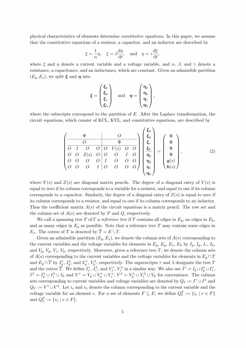
where the subscripts correspond to the partition of E. After the Laplace transformation, thecircuit equations, which consist of KCL, KVL, and constitutive equations, are described by

Ψ O

O ΦO I O O O Y (s) O O

O O Z(s) O O O I O

O O O O I O O O

O O O I O O O O

ξg

ξy

ξz

ξh

ηg

ηy

ηz

ηh

=

0000

g(s)h(s)

, (2)

where Y (s) and Z(s) are diagonal matrix pencils. The degree of a diagonal entry of Y (s) isequal to zero if its column corresponds to a variable for a resistor, and equal to one if its columncorresponds to a capacitor. Similarly, the degree of a diagonal entry of Z(s) is equal to zero ifits column corresponds to a resistor, and equal to one if its column corresponds to an inductor.Thus the coefficient matrix A(s) of the circuit equations is a matrix pencil. The row set andthe column set of A(s) are denoted by P and Q, respectively.

We call a spanning tree T of Γ a reference tree if T contains all edges in Eg, no edges in Eh,and as many edges in Ey as possible. Note that a reference tree T may contain some edges inEz. The cotree of T is denoted by T = E \ T .

Given an admissible partition (Ey, Ez), we denote the column sets of A(s) corresponding tothe current variables and the voltage variables for elements in Eg, Ey, Ez, Eh by Ig, Iy, Iz, Ih,and Vg, Vy, Vz, Vh, respectively. Moreover, given a reference tree T , we denote the column setsof A(s) corresponding to the current variables and the voltage variables for elements in Ey ∩T

and Ey ∩T by Iτy , Iλ

y , and V τy , V λ

y , respectively. The superscripts τ and λ designate the tree T

and the cotree T . We define Iτz , Iλ

z , and V τz , V λ

z in a similar way. We also use Iτ = Ig ∪ Iτy ∪ Iτ

z ,Iλ = Iλ

y ∪ Iλz ∪ Ih and V τ = Vg ∪ V τ

y ∪ V τz , V λ = V λ

y ∪ V λz ∪ Vh for convenience. The column

sets corresponding to current variables and voltage variables are denoted by QI := Iτ ∪ Iλ andQV := V τ ∪V λ. Let ie and ve denote the column corresponding to the current variable and thevoltage variable for an element e. For a set of elements F ⊆ E, we define QF

I := {ie | e ∈ F}and QF

V := {ve | e ∈ F}.

5

The row sets of A(s) corresponding to KCL, KVL, and constitutive equations are denotedby PI , PV , and S, respectively. Given an admissible partition (Ey, Ez) and a reference tree T ,let AT (s) be the coefficient matrix of the circuit equations, where Ψ is the fundamental cutsetmatrix and Φ is the fundamental loop matrix with respect to T . This means that we transformA(s) into AT (s) such that AT [PI , I

τ ] = I and AT [PV , V λ] = I by row operations in PI ∪ PV .Note that PI and Iτ as well as PV and V λ have one-to-one correspondence. The row sets ofAT (s) corresponding to Ig, Iτ

y , Iτz , and V λ

y , V λz , Vh are denoted by Pg, P τ

y , P τz , and P λ

y , P λz ,

Ph. If K ⊆ P and J ⊆ Q have the same superscript and subscript, AT [K, J ] is the unit matrix.Similarly, the row sets corresponding to Iy, Vz, Vg, and Ih are denoted by Sy, Sz, Sg, and Sh.By the definition of a reference tree, AT (s) has the following property.

Lemma 3.1 ([16, Lemma 3.1]). For a reference tree T , we have AT [P τz , Iλ

y ] = O and AT [P λy , V τ

z ] =O.

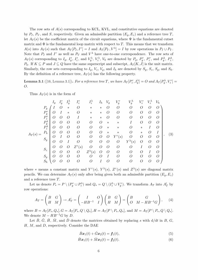
Thus AT (s) is in the form of

AT (s) =

Ig Iτy Iλ

y Iτz Iλ

z Ih Vg V τy V λ

y V τz V λ

z Vh

Pg I O ∗ O ∗ ∗ O O O O O O

P τy O I ∗ O ∗ ∗ O O O O O O

P τz O O O I ∗ ∗ O O O O O O

P λy O O O O O O ∗ ∗ I O O O

P λz O O O O O O ∗ ∗ O ∗ I O

Ph O O O O O O ∗ ∗ O ∗ O I

SyO

O

I

O

O

I

O

O

O

O

O

O

O

O

Y τ (s)O

O

Y λ(s)O

O

O

O

O

O

SzO

O

O

O

O

O

Zτ (s)O

O

Zλ(s)O

O

O

O

O

O

O

O

I

O

O

I

O

OSg O O O O O O I O O O O O

Sh O O O O O I O O O O O O

, (3)

where ∗ means a constant matrix and Y τ (s), Y λ(s), Zτ (s) and Zλ(s) are diagonal matrixpencils. We can determine AT (s) only after being given both an admissible partition (Ey, Ez)and a reference tree T .

Let us denote P∗ = P \ (P τy ∪ P λ

z ) and Q∗ = Q \ (Iλz ∪ V τ

y ). We transform AT into A′T byrow operations:

AT =

(B G

H M

)→ A′T =

(I O

−HB−1 I

)(B G

H M

)=

(B G

O M −HB−1G

), (4)

where B = AT [P∗, Q∗], G = AT [P∗, Q \Q∗],H = AT [P \ P∗, Q∗], and M = AT [P \ P∗, Q \Q∗].We denote M −HB−1G by D.

Let B, G, H, M , and D denote the matrices obtained by replacing s with d/dt in B, G,H, M , and D, respectively. Consider the DAE

Bx1(t) + Gx2(t) = f1(t), (5)

Hx1(t) + Mx2(t) = f2(t). (6)

6

By applying the transformation shown in (4), we obtain

Bx1(t) = f1(t)− Gx2(t), (7)

Dx2(t) = f2(t)− HB−1f1(t). (8)

We call the resulting DAE (8) the hybrid equations. Let us denote the vectors of currentscorresponding to Ig, Iτ

y , Iλy , Iτ

z , Iλz , Ih by ξg, ξτ

y , ξλy , ξτ

z , ξλz , ξh, and the vectors of voltages

corresponding to Vg, V τy , V λ

y , V τz , V λ

z , Vh by ηg, ητy , ηλ

y , ητz , ηλ

z , ηh. The procedure of thehybrid analysis is as follows.

1. The values of ξh and ηg are obvious from the equations corresponding to Sh and Sg.

2. Compute the values of ξλz and ητ

y by solving the hybrid equations (8).

3. Compute the values of ξτz and ηλ

y by substituting the values obtained in Steps 1–2 intothe equations corresponding to P τ

z and P λy .

4. Compute the values of ξτy , ξλ

y , ητz , and ηλ

z by substituting the values obtained in Steps 1–3into Sy and Sz.

5. Compute the values of ξg and ηh by substituting the values obtained in Steps 1–4 intoPg and Ph.

In the case of Ey = ∅, the above procedure is called the loop analysis or the tieset analysis.In the case of Ez = ∅, the procedure is called the cutset analysis.

All operations in Steps 3–5 are substitutions and differentiations of the obtained solutions.This is because we can transform B into an upper triangular matrix pencil with diagonal onesby permutations [16, Lemma 3.2]. Hence, the numerical difficulty is determined by the indexof the hybrid equations (8).

4 Index of Hybrid Equations

In this section, for linear time-invariant RLC circuits, we prove that the index ν(D) of the hybridequations is at most one, and we provide a necessary and sufficient condition for ν(D) = 0.

Given an admissible partition (Ey, Ez) and a reference tree T , consider the transformationshown in (4). For each p ∈ P and q ∈ Q, let dpq denote the degree of detAT [P \ {p}, Q \ {q}].The index ν(D) can be rewritten as follows.

Lemma 4.1 ([16, Lemma 4.1]). Given an admissible partition (Ey, Ez) and a reference treeT , the index of D is given by

ν(D) = maxp,q

{dpq | p ∈ P \ P∗, q ∈ Q \Q∗} − deg det AT + 1. (9)

The index of the hybrid equations has the following property.

Lemma 4.2 ([16, Theorem 4.4]). Given an admissible partition (Ey, Ez), the index ν(D) isthe same for any reference tree.

7

The generalized Laplace expansion applied to AT (s) results in

detAT =∑

F

sgnF det AT [PI , QFI ] detAT [PV , QF

V ] detAT [S,QFI ∪QF

V ], (10)

where the summation is over every spanning tree F of Γ which contains all edges in Eg but noedges in Eh, and sgnF is equal to +1 or −1. This is because AT [PI , Q

FI ] and AT [PV , QF

V ] arenonsingular due to the special structure of AT (s). It is known that detAT has the followingproperty.

Lemma 4.3 ([22, Theorem 2.5.1]). Each expansion term of det AT in (10) has the same sign.

For RLC circuits, we characterize deg detAT and dpq in terms of the number of inductors andcapacitors. Let R, L, and C denote the sets of resistors, inductors, and capacitors, respectively.We introduce a normal reference tree as follows.

Definition 4.4. A reference tree is called normal if it contains as many edges in C and as fewedges in L as possible.

The value of deg detAT for a normal reference tree T is expressed as follows.

Theorem 4.5. Given an admissible partition (Ey, Ez) and a normal reference tree T , we have

deg detAT = |T ∩ L|+ |T ∩ C|. (11)

Proof. Each expansion term aF (s) of detAT corresponding to a spanning tree F which containsall edges in Eg but no edges in Eh is given by

aF (s) = sgnF detAT [PI , QFI ] detAT [PV , QF

V ] detAT [S, QFI ∪QF

V ].

Since AT [S, QI ] and AT [S,QV ] are matrix pencils defined by (2), we have

deg aF (s) = |F ∩ L|+ |F ∩ C|.

By Definition 4.4, this implies that deg aF (s) ≤ deg aT (s) for any spanning tree F . ThenLemma 4.3 ensures that deg detAT = deg aT (s). Thus we obtain (11).

We now introduce the Resistor-Acyclic condition for admissible partition (Ey, Ez), which isproved in Theorem 4.9 to be a necessary and sufficient condition for ν(D) = 0.

[Resistor-Acyclic condition]

• Each e ∈ Ey ∩ R belongs to a cycle consisting of independent voltage sources,capacitors, and e.

• Each e ∈ Ez ∩ R belongs to a cutset consisting of inductors, independent currentsources, and e.

8

O

O

I

I

QFI QF

V

Pg

p

Sg

Sh

ikIg Ih Vg Vh

S

PV

PI

il = q vk vl

0

0

1

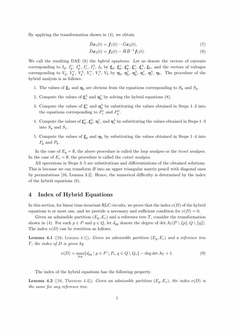
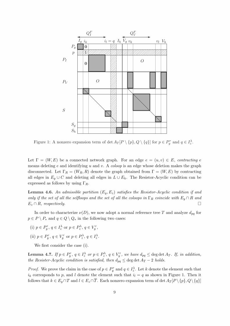
Figure 1: A nonzero expansion term of detAT [P \ {p}, Q \ {q}] for p ∈ P τy and q ∈ Iλ

z .

Let Γ = (W,E) be a connected network graph. For an edge e = (u, v) ∈ E, contracting e

means deleting e and identifying u and v. A coloop is an edge whose deletion makes the graphdisconnected. Let ΓR = (WR, R) denote the graph obtained from Γ = (W,E) by contractingall edges in Eg ∪ C and deleting all edges in L ∪ Eh. The Resistor-Acyclic condition can beexpressed as follows by using ΓR.

Lemma 4.6. An admissible partition (Ey, Ez) satisfies the Resistor-Acyclic condition if andonly if the set of all the selfloops and the set of all the coloops in ΓR coincide with Ey ∩R andEz ∩R, respectively.

In order to characterize ν(D), we now adopt a normal reference tree T and analyze dpq forp ∈ P \ P∗ and q ∈ Q \Q∗ in the following two cases:

(i) p ∈ P τy , q ∈ Iλ

z or p ∈ P λz , q ∈ V τ

y ,

(ii) p ∈ P τy , q ∈ V τ

y or p ∈ P λz , q ∈ Iλ

z .

We first consider the case (i).

Lemma 4.7. If p ∈ P τy , q ∈ Iλ

z or p ∈ P λz , q ∈ V τ

y , we have dpq ≤ deg detAT . If, in addition,the Resister-Acyclic condition is satisfied, then dpq ≤ deg detAT − 2 holds.

Proof. We prove the claim in the case of p ∈ P τy and q ∈ Iλ

z . Let k denote the element such thatik corresponds to p, and l denote the element such that il = q as shown in Figure 1. Then itfollows that k ∈ Ey∩T and l ∈ Ez∩T . Each nonzero expansion term of detAT [P \{p}, Q\{q}]

9

has one-to-one correspondence with spanning tree F of Γ such that F contains all edges inEg ∪ {k} but no edges in Eh ∪ {l}, and F \ {k} ∪ {l} is a spanning tree. Since AT [PI , {ik}] is aunit vector with the (p, ik) entry being one, AT [PI \ {p}, QF

I \ {ik}] is nonsingular. Thus, withrespect to F , detAT [P \ {p}, Q \ {q}] has a nonzero expansion term

aF (s) = detAT [PI \ {p}, QFI \ {ik}] detAT [PV , QF

V ∪ {vk} \ {vl}]det AT [S, (QF

I ∪ {ik} \ {il}) ∪ (QFV \ {vk} ∪ {vl})],

which is depicted in Figure 1. Let F maximize deg aF (s). Since aF (s) possibly disappears indetAT [P \ {p}, Q \ {q}] due to numerical cancellations, we have

dpq ≤ deg aF (s) = |L ∩ (F ∪ {k} \ {l})|+ |C ∩ (F \ {k} ∪ {l})|.

Note that k ∈ Ey implies that k is not an inductor and l ∈ Ez implies that l is not a capacitor.Hence we obtain

|L ∩ (F ∪ {k} \ {l})| = |L ∩ (F \ {l})| ≤ |L ∩ F | ≤ |L ∩ T |,

where T is a normal reference tree. Similarly |C ∩ (F \ {k} ∪ {l})| ≤ |C ∩ T | holds. Then itfollows from Theorem 4.5 that

dpq ≤ |L ∩ T |+ |C ∩ T | = deg detAT .

If (Ey, Ez) satisfies the Resistor-Acyclic condition, we have k ∈ Ey∩T ⊆ C and l ∈ Ez∩T ⊆L, which implies that |L∩ (F \ {l})| = |L∩F |− 1 and |C ∩ (F \ {k})| = |C ∩F |− 1. Therefore,dpq ≤ deg det AT − 2 holds.

In the case of p ∈ P λz , q ∈ V τ

y , the claim is proved in a similar way.

Next, we consider the case (ii).

Lemma 4.8. If p ∈ P τy , q ∈ V τ

y or p ∈ P λz , q ∈ Iλ

z , we have dpq ≤ deg detAT . If, in addition,the Resister-Acyclic condition is satisfied, then dpq ≤ deg detAT − 1 holds.

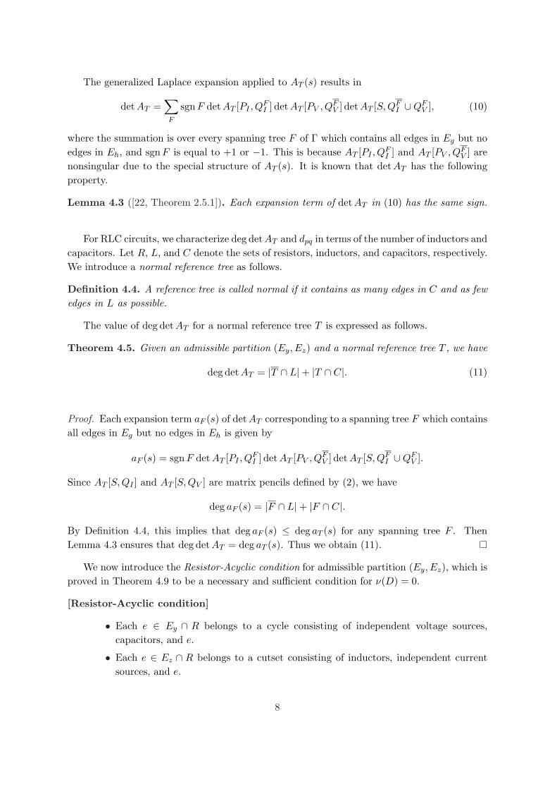
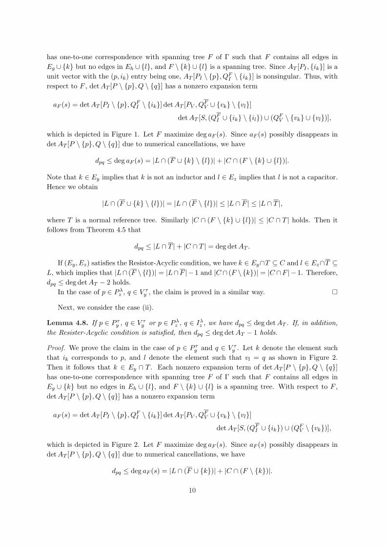
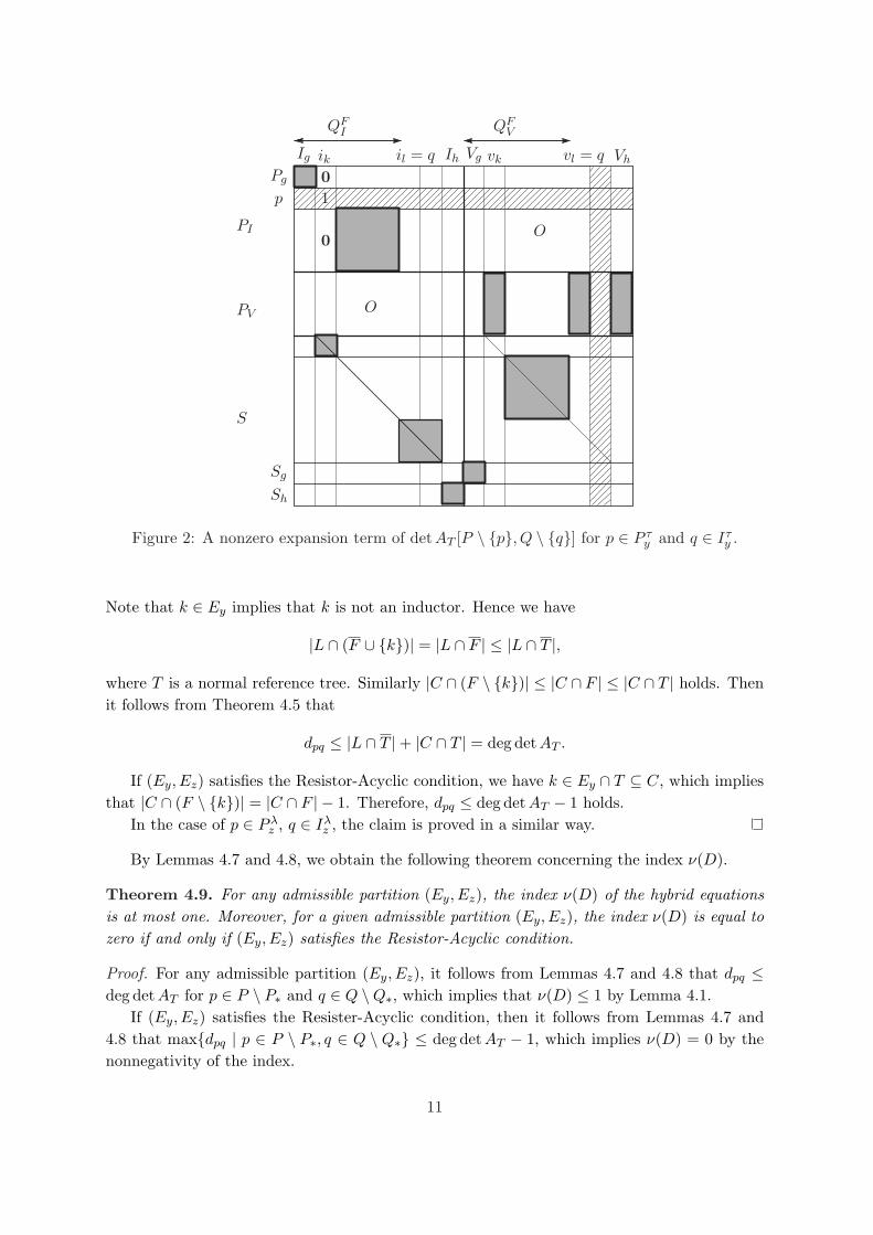
Proof. We prove the claim in the case of p ∈ P τy and q ∈ V τ

y . Let k denote the element suchthat ik corresponds to p, and l denote the element such that vl = q as shown in Figure 2.Then it follows that k ∈ Ey ∩ T . Each nonzero expansion term of detAT [P \ {p}, Q \ {q}]has one-to-one correspondence with spanning tree F of Γ such that F contains all edges inEg ∪ {k} but no edges in Eh ∪ {l}, and F \ {k} ∪ {l} is a spanning tree. With respect to F ,detAT [P \ {p}, Q \ {q}] has a nonzero expansion term

aF (s) = detAT [PI \ {p}, QFI \ {ik}] detAT [PV , QF

V ∪ {vk} \ {vl}]det AT [S, (QF

I ∪ {ik}) ∪ (QFV \ {vk})],

which is depicted in Figure 2. Let F maximize deg aF (s). Since aF (s) possibly disappears indetAT [P \ {p}, Q \ {q}] due to numerical cancellations, we have

dpq ≤ deg aF (s) = |L ∩ (F ∪ {k})|+ |C ∩ (F \ {k})|.

10

O

O

I

I

QFI QF

V

Pg

p

Sg

Sh

ikIg Ih Vg Vh

S

PV

PI

il = q vk vl = q

0

0

1

Figure 2: A nonzero expansion term of detAT [P \ {p}, Q \ {q}] for p ∈ P τy and q ∈ Iτ

y .

Note that k ∈ Ey implies that k is not an inductor. Hence we have

|L ∩ (F ∪ {k})| = |L ∩ F | ≤ |L ∩ T |,

where T is a normal reference tree. Similarly |C ∩ (F \ {k})| ≤ |C ∩ F | ≤ |C ∩ T | holds. Thenit follows from Theorem 4.5 that

dpq ≤ |L ∩ T |+ |C ∩ T | = deg detAT .

If (Ey, Ez) satisfies the Resistor-Acyclic condition, we have k ∈ Ey ∩ T ⊆ C, which impliesthat |C ∩ (F \ {k})| = |C ∩ F | − 1. Therefore, dpq ≤ deg det AT − 1 holds.

In the case of p ∈ P λz , q ∈ Iλ

z , the claim is proved in a similar way.

By Lemmas 4.7 and 4.8, we obtain the following theorem concerning the index ν(D).

Theorem 4.9. For any admissible partition (Ey, Ez), the index ν(D) of the hybrid equationsis at most one. Moreover, for a given admissible partition (Ey, Ez), the index ν(D) is equal tozero if and only if (Ey, Ez) satisfies the Resistor-Acyclic condition.

Proof. For any admissible partition (Ey, Ez), it follows from Lemmas 4.7 and 4.8 that dpq ≤deg detAT for p ∈ P \ P∗ and q ∈ Q \Q∗, which implies that ν(D) ≤ 1 by Lemma 4.1.

If (Ey, Ez) satisfies the Resister-Acyclic condition, then it follows from Lemmas 4.7 and4.8 that max{dpq | p ∈ P \ P∗, q ∈ Q \ Q∗} ≤ deg det AT − 1, which implies ν(D) = 0 by thenonnegativity of the index.

11

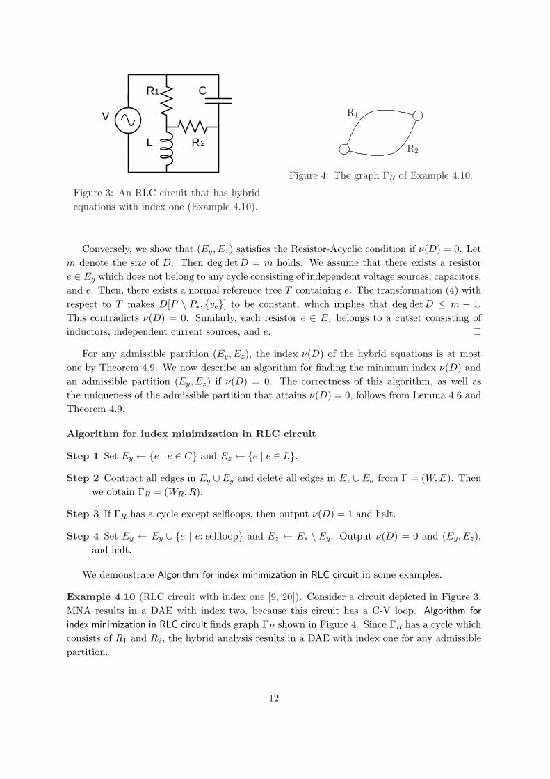
R C

V

L R

1

2

Figure 3: An RLC circuit that has hybridequations with index one (Example 4.10).

R1

R2

Figure 4: The graph ΓR of Example 4.10.

Conversely, we show that (Ey, Ez) satisfies the Resistor-Acyclic condition if ν(D) = 0. Letm denote the size of D. Then deg detD = m holds. We assume that there exists a resistore ∈ Ey which does not belong to any cycle consisting of independent voltage sources, capacitors,and e. Then, there exists a normal reference tree T containing e. The transformation (4) withrespect to T makes D[P \ P∗, {ve}] to be constant, which implies that deg detD ≤ m − 1.This contradicts ν(D) = 0. Similarly, each resistor e ∈ Ez belongs to a cutset consisting ofinductors, independent current sources, and e.

For any admissible partition (Ey, Ez), the index ν(D) of the hybrid equations is at mostone by Theorem 4.9. We now describe an algorithm for finding the minimum index ν(D) andan admissible partition (Ey, Ez) if ν(D) = 0. The correctness of this algorithm, as well asthe uniqueness of the admissible partition that attains ν(D) = 0, follows from Lemma 4.6 andTheorem 4.9.

Algorithm for index minimization in RLC circuit

Step 1 Set Ey ← {e | e ∈ C} and Ez ← {e | e ∈ L}.

Step 2 Contract all edges in Eg ∪Ey and delete all edges in Ez ∪Eh from Γ = (W,E). Thenwe obtain ΓR = (WR, R).

Step 3 If ΓR has a cycle except selfloops, then output ν(D) = 1 and halt.

Step 4 Set Ey ← Ey ∪ {e | e: selfloop} and Ez ← E∗ \ Ey. Output ν(D) = 0 and (Ey, Ez),and halt.

We demonstrate Algorithm for index minimization in RLC circuit in some examples.

Example 4.10 (RLC circuit with index one [9, 20]). Consider a circuit depicted in Figure 3.MNA results in a DAE with index two, because this circuit has a C-V loop. Algorithm for

index minimization in RLC circuit finds graph ΓR shown in Figure 4. Since ΓR has a cycle whichconsists of R1 and R2, the hybrid analysis results in a DAE with index one for any admissiblepartition.

12

V

C

L

L

R

R

1

2

1

2

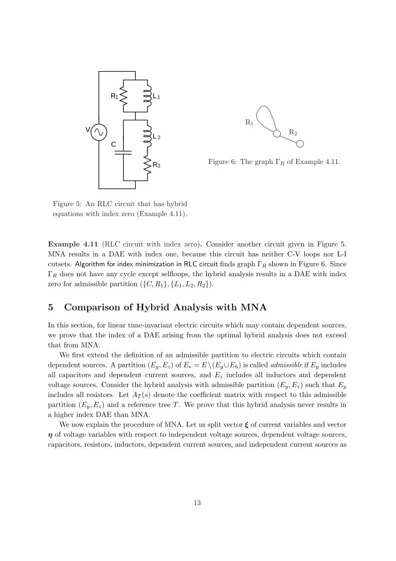
Figure 5: An RLC circuit that has hybridequations with index zero (Example 4.11).

R1

R2

Figure 6: The graph ΓR of Example 4.11.

Example 4.11 (RLC circuit with index zero). Consider another circuit given in Figure 5.MNA results in a DAE with index one, because this circuit has neither C-V loops nor L-Icutsets. Algorithm for index minimization in RLC circuit finds graph ΓR shown in Figure 6. SinceΓR does not have any cycle except selfloops, the hybrid analysis results in a DAE with indexzero for admissible partition ({C, R1}, {L1, L2, R2}).

5 Comparison of Hybrid Analysis with MNA

In this section, for linear time-invariant electric circuits which may contain dependent sources,we prove that the index of a DAE arising from the optimal hybrid analysis does not exceedthat from MNA.

We first extend the definition of an admissible partition to electric circuits which containdependent sources. A partition (Ey, Ez) of E∗ = E\(Eg∪Eh) is called admissible if Ey includesall capacitors and dependent current sources, and Ez includes all inductors and dependentvoltage sources. Consider the hybrid analysis with admissible partition (Ey, Ez) such that Ey

includes all resistors. Let AT (s) denote the coefficient matrix with respect to this admissiblepartition (Ey, Ez) and a reference tree T . We prove that this hybrid analysis never results ina higher index DAE than MNA.

We now explain the procedure of MNA. Let us split vector ξ of current variables and vectorη of voltage variables with respect to independent voltage sources, dependent voltage sources,capacitors, resistors, inductors, dependent current sources, and independent current sources as

13

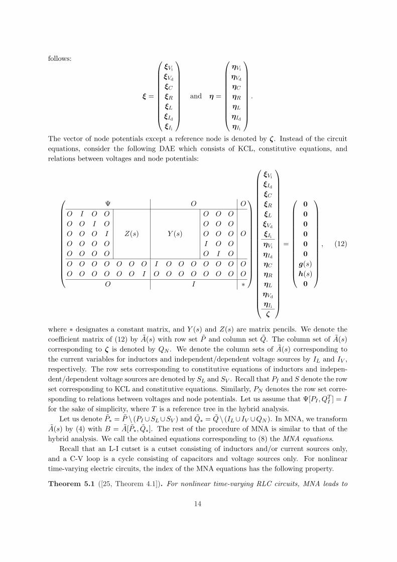
follows:

ξ =

ξVi

ξVd

ξC

ξR

ξL

ξId

ξIi

and η =

ηVi

ηVd

ηC

ηR

ηL

ηId

ηIi

.

The vector of node potentials except a reference node is denoted by ζ. Instead of the circuitequations, consider the following DAE which consists of KCL, constitutive equations, andrelations between voltages and node potentials:

Ψ O O

O

O

O

O

O

I

O

O

O

O

O

I

O

O

O

O

O

I

O

O

Z(s) Y (s)

O

O

O

I

O

O

O

O

O

I

O

O

O

O

O

O

O O O O O O O I O O O O O O O

O O O O O O I O O O O O O O O

O I ∗

ξVi

ξId

ξC

ξR

ξL

ξVd

ξIi

ηVi

ηId

ηC

ηR

ηL

ηVd

ηIi

ζ

=

000000

g(s)h(s)0

, (12)

where ∗ designates a constant matrix, and Y (s) and Z(s) are matrix pencils. We denote thecoefficient matrix of (12) by A(s) with row set P and column set Q. The column set of A(s)corresponding to ζ is denoted by QN . We denote the column sets of A(s) corresponding tothe current variables for inductors and independent/dependent voltage sources by IL and IV ,respectively. The row sets corresponding to constitutive equations of inductors and indepen-dent/dependent voltage sources are denoted by SL and SV . Recall that PI and S denote the rowset corresponding to KCL and constitutive equations. Similarly, PN denotes the row set corre-sponding to relations between voltages and node potentials. Let us assume that Ψ[PI , Q

TI ] = I

for the sake of simplicity, where T is a reference tree in the hybrid analysis.Let us denote P∗ = P \ (PI ∪SL∪SV ) and Q∗ = Q\ (IL∪ IV ∪QN ). In MNA, we transform

A(s) by (4) with B = A[P∗, Q∗]. The rest of the procedure of MNA is similar to that of thehybrid analysis. We call the obtained equations corresponding to (8) the MNA equations.

Recall that an L-I cutset is a cutset consisting of inductors and/or current sources only,and a C-V loop is a cycle consisting of capacitors and voltage sources only. For nonlineartime-varying electric circuits, the index of the MNA equations has the following property.

Theorem 5.1 ([25, Theorem 4.1]). For nonlinear time-varying RLC circuits, MNA leads to

14

a DAE with index one if and only if the network contains neither L-I cutsets nor C-V loops.Otherwise, MNA leads to a DAE with index two.

This theorem is generalized for nonlinear time-varying electric circuits containing dependentsources which satisfy certain conditions [25]. Theorem 5.1 implies that the index of the MNAequations is at least one. On the other hand, for RLC circuits, the index of the hybrid equationsis at most one by Theorem 4.9. Hence, the index of the hybrid equations does not exceed thatof the MNA equations for linear time-invariant RLC circuits. In the rest of this paper, wegeneralize this for linear time-invariant electric circuits which may contain dependent sources.

For any square submatrix A[K, J ], we write w(K, J) = deg detA[K, J ], where w(∅, ∅) = 0by convention. Then, w(K, J) enjoys the following property.

Lemma 5.2 ([20, pp. 287–289]). Let A(s) be a matrix pencil with row set P and column setQ. For any (K, J) ∈ Λ, (K ′, J ′) ∈ Λ, where Λ = {(K,J) | |K| = |J |, K ⊆ P, J ⊆ Q}, both(VB-1) and (VB-2) below hold:

(VB-1) For any k ∈ K \K ′, at least one of the following two statements holds:

(1a) ∃j ∈ J \ J ′ : w(K,J) + w(K ′, J ′) ≤ w(K \ {k}, J \ {j}) + w(K ′ ∪ {k}, J ′ ∪ {j}),(1b) ∃h ∈ K ′ \K : w(K, J) + w(K ′, J ′) ≤ w(K \ {k} ∪ {h}, J) + w(K ′ \ {h} ∪ {k}, J ′).

(VB-2) For any j ∈ J \ J ′, at least one of the following two statements holds:

(2a) ∃k ∈ K \K ′ : w(K,J) + w(K ′, J ′) ≤ w(K \ {k}, J \ {j}) + w(K ′ ∪ {k}, J ′ ∪ {j}),(2b) ∃l ∈ J ′ \ J : w(K, J) + w(K ′, J ′) ≤ w(K,J \ {j} ∪ {l}) + w(K ′, J ′ \ {l} ∪ {j}).

We denote dpq = deg det A[P \ {p}, Q \ {q}] for p ∈ P and q ∈ Q. Similarly to Lemma 4.1,the index ν of the MNA equations is given by

ν = maxp,q

{dpq | p ∈ P \ P∗, q ∈ Q \ Q∗} − deg det A + 1. (13)

In order to compare ν with ν(D), we show the relation between A(s) and AT (s) in thefollowing lemma.

Lemma 5.3. For the matrix pencils A(s) and AT (s), it holds that det A(s) = ±detAT (s).Moreover, we have dpq = dpq for p ∈ P \ P∗ and q ∈ Q \Q∗.

Proof. Let PV denote the column set such that PV ⊆ PN and A[PV , QTV ] = I. We transform

A(s) into

A′(s) =

PI

S

PV

PN \ PV

Ψ O O O

constitutive eq. O

O O ∗ I O

O O ∗ O I

by elementary row operations on PN without adding multiples of rows in PV to any rows.Then PV corresponds to KVL. Since it holds that A′[P \ (PN \ PV ), Q \ QN ] = AT , we havedet A(s) = ±det A′(s) = ±det AT (s). This transformation does not change the value of dpq

for any p ∈ PI ∪ PV and q ∈ Q \ QN . Hence we have dpq = deg det A′[P \ {p}, Q \ {q}] = dpq

for p ∈ P \ P∗ and q ∈ Q \Q∗.

15

QNIL IVV τ

y

Iλz

P τy

P λz

V λz

PN

PI

QI QV

SL

SV

PV

S

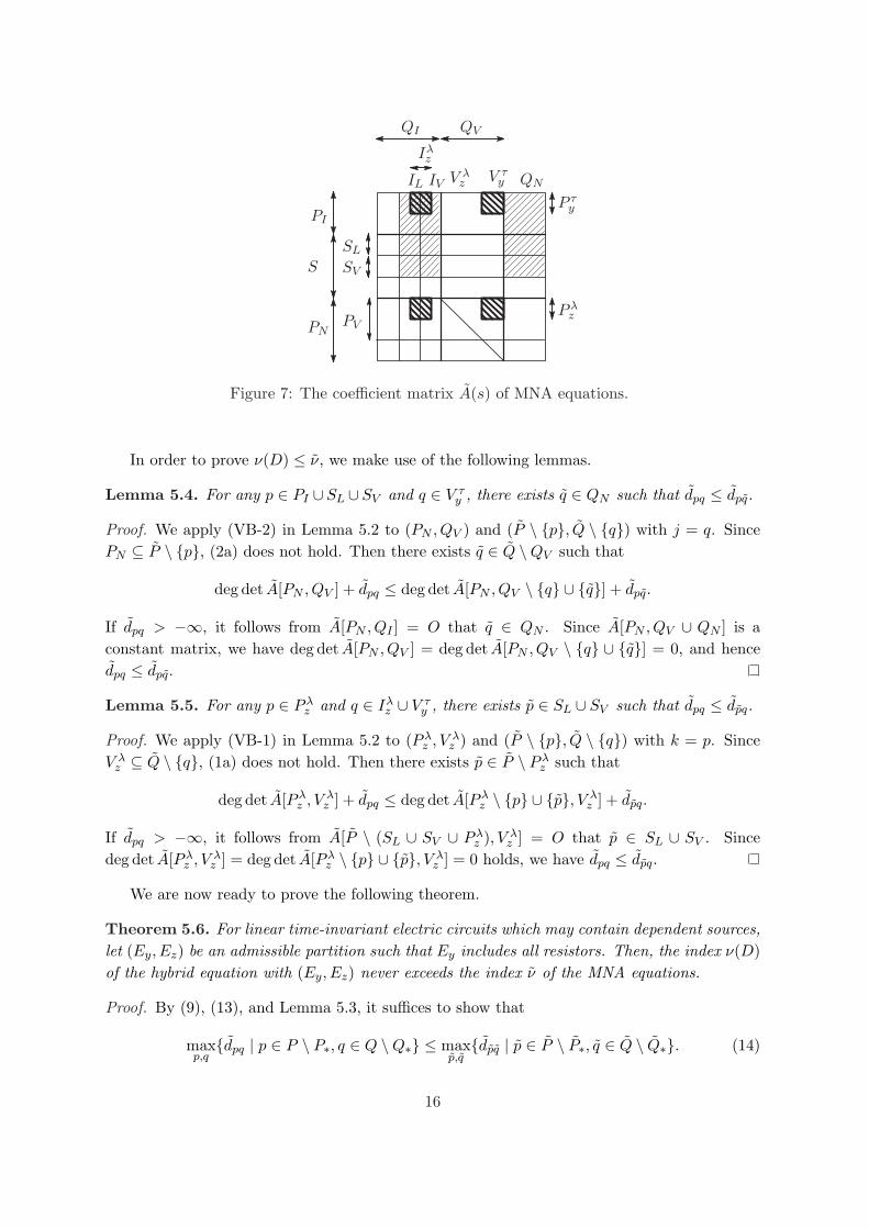
Figure 7: The coefficient matrix A(s) of MNA equations.

In order to prove ν(D) ≤ ν, we make use of the following lemmas.

Lemma 5.4. For any p ∈ PI ∪SL ∪ SV and q ∈ V τy , there exists q ∈ QN such that dpq ≤ dpq.

Proof. We apply (VB-2) in Lemma 5.2 to (PN , QV ) and (P \ {p}, Q \ {q}) with j = q. SincePN ⊆ P \ {p}, (2a) does not hold. Then there exists q ∈ Q \QV such that

deg det A[PN , QV ] + dpq ≤ deg det A[PN , QV \ {q} ∪ {q}] + dpq.

If dpq > −∞, it follows from A[PN , QI ] = O that q ∈ QN . Since A[PN , QV ∪ QN ] is aconstant matrix, we have deg det A[PN , QV ] = deg det A[PN , QV \ {q} ∪ {q}] = 0, and hencedpq ≤ dpq.

Lemma 5.5. For any p ∈ P λz and q ∈ Iλ

z ∪ V τy , there exists p ∈ SL ∪ SV such that dpq ≤ dpq.

Proof. We apply (VB-1) in Lemma 5.2 to (P λz , V λ

z ) and (P \ {p}, Q \ {q}) with k = p. SinceV λ

z ⊆ Q \ {q}, (1a) does not hold. Then there exists p ∈ P \ P λz such that

deg det A[P λz , V λ

z ] + dpq ≤ deg det A[P λz \ {p} ∪ {p}, V λ

z ] + dpq.

If dpq > −∞, it follows from A[P \ (SL ∪ SV ∪ P λz ), V λ

z ] = O that p ∈ SL ∪ SV . Sincedeg det A[P λ

z , V λz ] = deg det A[P λ

z \ {p} ∪ {p}, V λz ] = 0 holds, we have dpq ≤ dpq.

We are now ready to prove the following theorem.

Theorem 5.6. For linear time-invariant electric circuits which may contain dependent sources,let (Ey, Ez) be an admissible partition such that Ey includes all resistors. Then, the index ν(D)of the hybrid equation with (Ey, Ez) never exceeds the index ν of the MNA equations.

Proof. By (9), (13), and Lemma 5.3, it suffices to show that

maxp,q

{dpq | p ∈ P \ P∗, q ∈ Q \Q∗} ≤ maxp,q

{dpq | p ∈ P \ P∗, q ∈ Q \ Q∗}. (14)

16

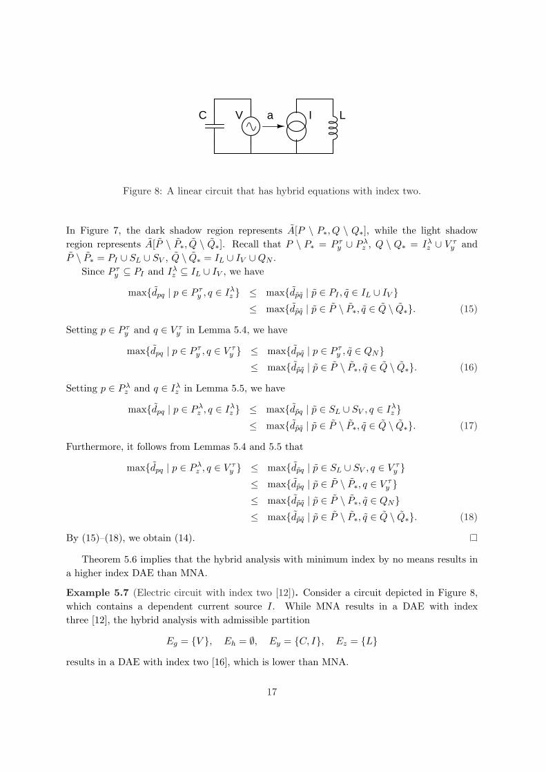
C aV I L

Figure 8: A linear circuit that has hybrid equations with index two.

In Figure 7, the dark shadow region represents A[P \ P∗, Q \ Q∗], while the light shadowregion represents A[P \ P∗, Q \ Q∗]. Recall that P \ P∗ = P τ

y ∪ P λz , Q \ Q∗ = Iλ

z ∪ V τy and

P \ P∗ = PI ∪ SL ∪ SV , Q \ Q∗ = IL ∪ IV ∪QN .Since P τ

y ⊆ PI and Iλz ⊆ IL ∪ IV , we have

max{dpq | p ∈ P τy , q ∈ Iλ

z } ≤ max{dpq | p ∈ PI , q ∈ IL ∪ IV }≤ max{dpq | p ∈ P \ P∗, q ∈ Q \ Q∗}. (15)

Setting p ∈ P τy and q ∈ V τ

y in Lemma 5.4, we have

max{dpq | p ∈ P τy , q ∈ V τ

y } ≤ max{dpq | p ∈ P τy , q ∈ QN}

≤ max{dpq | p ∈ P \ P∗, q ∈ Q \ Q∗}. (16)

Setting p ∈ P λz and q ∈ Iλ

z in Lemma 5.5, we have

max{dpq | p ∈ P λz , q ∈ Iλ

z } ≤ max{dpq | p ∈ SL ∪ SV , q ∈ Iλz }

≤ max{dpq | p ∈ P \ P∗, q ∈ Q \ Q∗}. (17)

Furthermore, it follows from Lemmas 5.4 and 5.5 that

max{dpq | p ∈ P λz , q ∈ V τ

y } ≤ max{dpq | p ∈ SL ∪ SV , q ∈ V τy }

≤ max{dpq | p ∈ P \ P∗, q ∈ V τy }

≤ max{dpq | p ∈ P \ P∗, q ∈ QN}≤ max{dpq | p ∈ P \ P∗, q ∈ Q \ Q∗}. (18)

By (15)–(18), we obtain (14).

Theorem 5.6 implies that the hybrid analysis with minimum index by no means results ina higher index DAE than MNA.

Example 5.7 (Electric circuit with index two [12]). Consider a circuit depicted in Figure 8,which contains a dependent current source I. While MNA results in a DAE with indexthree [12], the hybrid analysis with admissible partition

Eg = {V }, Eh = ∅, Ey = {C, I}, Ez = {L}results in a DAE with index two [16], which is lower than MNA.

17

6 Conclusion

For linear time-invariant RLC circuits, we have proved that the index of the hybrid equationsnever exceeds one, and given a structural characterization of circuits with index zero. The proofmakes use of the special property of RLC circuits that the coefficient matrix of constitutiveequations consists of diagonal matrix pencils. Moreover, the structural characterization hasbrought an index minimization algorithm, which is much faster and simpler than the previousone developed in [16]. Finally, for linear time-invariant electric circuits which may containdependent sources, we have shown that the minimum index of hybrid equations does not exceedthe index of MNA equations, which suggests that the hybrid analysis is superior to MNA innumerical accuracy. Extending these results to nonlinear/time-varying electric circuits is leftfor future investigation.

References

[1] S. Amari: Topological foundations of Kron’s tearing of electric networks, RAAG Memoirs,vol.3, F-VI, pp. 322–350, 1962.

[2] S. Bachle: Index reduction for differential-algebraic equations in circuit simulation, MATH-EON 141, Technical University of Berlin, 2004.

[3] S. Bachle and F. Ebert: Graph theoretical algorithms for index reduction in circuit simu-lation, MATHEON 245, Technical University of Berlin, 2004.

[4] S. Bachle and F. Ebert: Element-based index reduction in electrical circuit simulation,Proceedings in Applied Mathematics and Mechanics, vol. 6, pp. 731–732, 2006.

[5] F. H. Branin: The relation between Kron’s method and the classical methods of networkanalysis, The Matrix and Tensor Quarterly, vol. 12, pp. 69–115, 1962.

[6] K. E. Brenan, S. L. Campbell, and L. R. Petzold: Numerical Solution of Initial-ValueProblems in Differential-Algebraic Equations, SIAM, Philadelphia, 2nd edition, 1996.

[7] P. Bujakiewicz: Maximum Weighted Matching for High Index Differential Algebraic Equa-tions, Doctor’s dissertation, Delft University of Technology, 1994.

[8] S. L. Campbell and C. W. Gear: The index of general nonlinear DAEs, NumerischeMathematik, vol. 72, pp. 173–196, 1995.

[9] F. E. Cellier: Continuous System Modeling, Springer-Verlag, Berlin, 1991.

[10] F. R. Gantmacher: The Theory of Matrices, Chelsea, New York, 1959.

[11] C. W. Gear: Simultaneous numerical solution of differential-algebraic equations, IEEETransactions on Circuit Theory, vol. 18, pp. 89–95, 1971.

[12] M. Gunther and P. Rentrop: The differential-algebraic index concept in electric circuitsimulation, Zeitschrift fur angewandte Mathematik und Mechanik, vol. 76, supplement 1,pp. 91–94, 1996.

18

[13] E. Hairer and G. Wanner: Solving Ordinary Differential Equations II, Springer-Verlag,Berlin, 2nd edition, 1996.

[14] M. Iri: A min-max theorem for the ranks and term-ranks of a class of matrices: Analgebraic approach to the problem of the topological degrees of freedom of a network (inJapanese), Transactions of the Institute of Electronics and Communication Engineers ofJapan, vol. 51A, pp. 180–187, 1968.

[15] M. Iri: Applications of Matroid Theory, Mathematical Programming — The State of theArt, Springer-Verlag, Berlin, pp. 158–201, 1983.

[16] S. Iwata and M. Takamatsu: Index minimization of differential-algebraic equations inhybrid analysis for circuit simulation, METR 2007-33, Department of Mathematical In-formatics, University of Tokyo, May 2007.

[17] G. Kishi and Y. Kajitani: Maximally distinct trees in a linear graph (in Japanese), Trans-actions of the Institute of Electronics and Communication Engineers of Japan, vol. 51A,pp. 196–203, 1968.

[18] G. Kron: Tensor Analysis of Networks, John Wiley and Sons, New York, 1939.

[19] R. Marz: Numerical methods for differential-algebraic equations, Acta Numerica, vol. 1,pp. 141–198, 1992.

[20] K. Murota: Matrices and Matroids for Systems Analysis, Springer-Verlag, Berlin, 2000.

[21] T. Ohtsuki, Y. Ishizaki, and H. Watanabe: Network analysis and topological degrees offreedom (in Japanese), Transactions of the Institute of Electronics and CommunicationEngineers of Japan, vol. 51A, pp. 238–245, 1968.

[22] A. Recski: Matroid Theory and Its Applications in Electric Network Theory and in Statics,Springer-Verlag, Berlin, 1989.

[23] S. Schulz: Four lectures on differential-algebraic equations, Technical Report 497, TheUniversity of Auckland, New Zealand, 2003.

[24] D. E. Schwarz: Consistent initialization for index-2 differential algebraic equations and itsapplication to circuit simulation, Ph.D. thesis, Humboldt University, Berlin, 2000.

[25] D. E. Schwarz and C. Tischendorf: Structural analysis of electric circuits and consequencesfor MNA, International Journal of Circuit Theory and Applications, vol. 28, pp. 131–162,2000.

[26] C. Tischendorf: Topological index calculation of differential-algebraic equations in circuitsimulation, Surveys on Mathematics for Industry, vol. 8, pp.187–199, 1999.

19