Mathematical Economics Lecture 1 · 2019-10-02 · Mathematical Economics Lecture 1 Dr Wioletta...
62
Mathematical Economics Lecture 1 Dr Wioletta Nowak, room 205 C [email protected] http://prawo.uni.wroc.pl/user/12141/students-resources
Transcript of Mathematical Economics Lecture 1 · 2019-10-02 · Mathematical Economics Lecture 1 Dr Wioletta...
Mathematical Economics
Lecture 1
Dr Wioletta Nowak, room 205 C [email protected]
http://prawo.uni.wroc.pl/user/12141/students-resources

Syllabus
Mathematical Theory of Demand
Utility Maximization Problem
Expenditure Minimization Problem
Mathematical Theory of Production
Profit Maximization Problem
Cost Minimization Problem
General Equilibrium Theory
Growth Models
Dynamic Optimization

Syllabus
Mathematical Theory of Demand
• Budget Constraint
• Consumer Preferences
• Utility Function
• Utility Maximization Problem
• Optimal Choice
• Properties of Demand Function
• Indirect Utility Function and its Properties
• Roy’s Identity

Syllabus
Mathematical Theory of Demand
• Expenditure Minimization Problem
• Expenditure Function and its Properties
• Shephard's Lemma
• Properties of Hicksian Demand Function
• The Compensated Law of Demand
• Relationship between Utility Maximization and Expenditure Minimization Problem

Syllabus
Mathematical Theory of Production
• Production Functions and Their Properties
• Perfectly Competitive Firms
• Profit Function and Profit Maximization
Problem
• Properties of Input Demand and Output
Supply Functions

Syllabus
Mathematical Theory of Production
• Cost Minimization Problem
• Definition and Properties of Conditional Factor Demand and Cost Function
• Profit Maximization with Cost Function
• Long and Short Run Equilibrium
• Total Costs, Average Costs, Marginal Costs, Long-run Costs, Short-run Costs, Cost Curves, Long-run and Short-run Cost Curves
Syllabus
Mathematical Theory of Production
Monopoly
Oligopoly
• Cournot Equilibrium
• Quantity Leadership – Slackelberg Model

Syllabus
General Equilibrium Theory
• Exchange
• Market Equilibrium

Syllabus
Neoclassical Growth Model
• The Solow Growth Model
• Introduction to Dynamic Optimization
• The Ramsey-Cass-Koopmans Growth Model
Models of Endogenous Growth Theory
Convergence to the Balance Growth Path

Recommended Reading
• Chiang A.C., Wainwright K., Fundamental Methods of Mathematical Economics, McGraw-Hill/Irwin, Boston, Mass., (4th edition) 2005.
• Chiang A.C., Elements of Dynamic Optimization, Waveland Press, 1992.
• Romer D., Advanced Macroeconomics, McGraw-Hill, 1996.
• Varian H.R., Intermediate Microeconomics, A Modern Approach, W.W. Norton & Company, New York, London, 1996.

The Theory of Consumer Choice
• The Budget Constraint
• The Budget Line Changes (Increasing Income, Increasing Price)
• Consumer Preferences
• Assumptions about Preferences
• Indifference Curves: Normal Good, Substitutes, Complements, Bads, Neutrals
• The Marginal Rate of Substitution

Consumers choose the best bundle of
goods they can afford
• How to describe what a consumer can afford?
• What does mean the best bundle?
• The consumer theory uses the concepts of a
budget constraint and a preference map to
analyse consumer choices.

The budget constraint – the two-good case
• It represents the combination of goods that
consumer can purchase given current prices
and income.
• - consumer’s
consumption bundle (the object of consumer
choice)
• - market prices
of the goods
2,1i,0x,x,x i21
2,1i,0p,p,p i21

The budget constraint – the two-good case
• The budget constraint of the consumer (the amount of money spent on the two goods is no more than the total amount the consumer has to spend)
• - consumer’s income (the amount of money the
consumer has to spend)
• - the amount of money the consumer is spending on good 1
• - the amount of money the consumer is spending on good 2
Ixpxp 2211
11xp
22xp
0I

Graphical representation of the budget set and the budget line
• The set of affordable consumption bundles at given prices and income is called the budget set of the consumer.

The Budget Line

The Budget Line Changes
• Increasing (decreasing) income – an increase (decrease) in
income causes a parallel shift outward (inward) of the budget
line (a lump-sum tax; a value tax)

The Budget Line Changes
• Increasing price – if good 1 becomes more expensive, the budget line becomes steeper.
• Increasing the price of good 1 makes the budget line steeper; increasing the price of good 2 makes the budget line flatter.
• A quantity tax (excise)
A value tax (ad valorem tax)
A quantity subsidy
Ad valorem subsidy

Exercise 1

Consumer Preferences

Consumer Preferences
preferenceweakofrelationyxXX)y,x(P
ofrelationy~xXX)y,x(I
preferencestrictofrelationyxXX)y,x(P
~
s
ceindifferen

Assumptions about Preferences

Assumptions about Preferences

Assumptions about Preferences

Assumptions about Preferences

The relations of strict preference, weak preference and
indifference are not independent concepts!


Exercise 2

Exercise 3
Indifference Curves
• The set of all consumption bundles that are
indifferent to each other is called an
indifference curve.
• Points yielding different utility levels are each
associated with distinct indifference curves.

Indifference curves are

Indifference curve for normal goods

Substitutes
• Two goods are substitutes if the consumer is willing to substitute one good for the other at a constant rate.
• The case of perfect substitutes occurs when the consumer is willing to substitute the goods on a one-to-one basis.
• The indifference curves has a constant slope since the consumer is willing to trade at a fixed ratio.
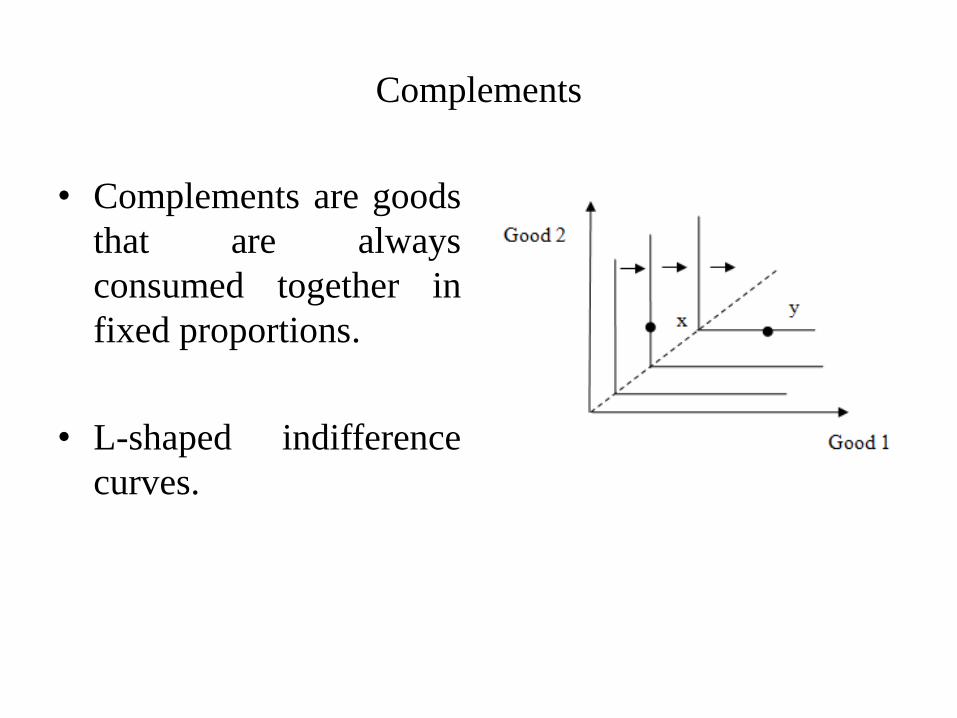
Complements
• Complements are goods
that are always
consumed together in
fixed proportions.
• L-shaped indifference
curves.

Bads: a bad is a commodity that consumer doesn’t like

Neutrals: a good is a neutral good if the consumer
doesn’t care about it one way or the other

The Marginal Rate of Substitution (MRS)
• The marginal rate of substitution measures the slope of the
indifference curve.

The Marginal Rate of Substitution (MRS)

The Marginal Rate of Substitution (MRS)
• The MRS is different at each point along the
indifference curve for normal goods.
• The marginal rate of substitution between
perfect substitutes is constant.

Mathematical Economics dr Wioletta Nowak
Lecture 2

• The Utility Function,
• Examples of Utility Functions: Normal Good, Perfect Substitutes, Perfect Complements,
• The Quasilinear and Homothetic Utility Functions,
• The Marginal Utility and The Marginal Rate of Substitution,
• The Optimal Choice,
• The Utility Maximization Problem,
• The Lagrange Method

The Utility Function
• A utility is a measure of the relative
satisfaction from consumption of various
goods.
• A utility function is a way of assigning a
number to every possible consumption bundle
such that more-preferred bundles get assigned
larger numbers then less-preferred bundles.

The Utility Function
• The numerical magnitudes of utility levels have no intrinsic meaning – the only property of a utility assignment that is important is how it orders the bundles of goods.
• The magnitude of the utility function is only important insofar as it ranks the different consumption bundles.
• Ordinal utility - consumer assigns a higher utility to the chosen bundle than to the rejected. Ordinal utility captures only ranking and not strength of preferences.
• Cardinal utility theories attach a significance to the magnitude of utility. The size of the utility difference between two bundles of goods is supposed to have some sort of significance.

Existence of a Utility Function
• Suppose preferences are complete, reflexive,
transitive, continuous, and strongly monotonic.
• Then there exists a continuous utility function
which represents those preferences.
2:u
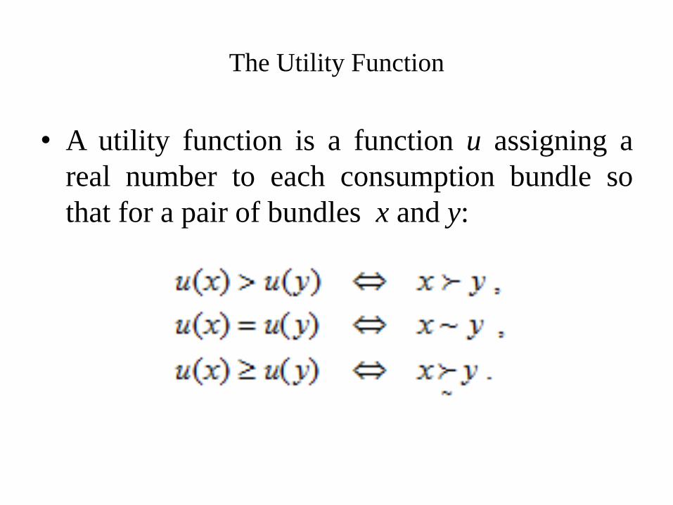
The Utility Function
• A utility function is a function u assigning a
real number to each consumption bundle so
that for a pair of bundles x and y:

Examples of Utility Functions
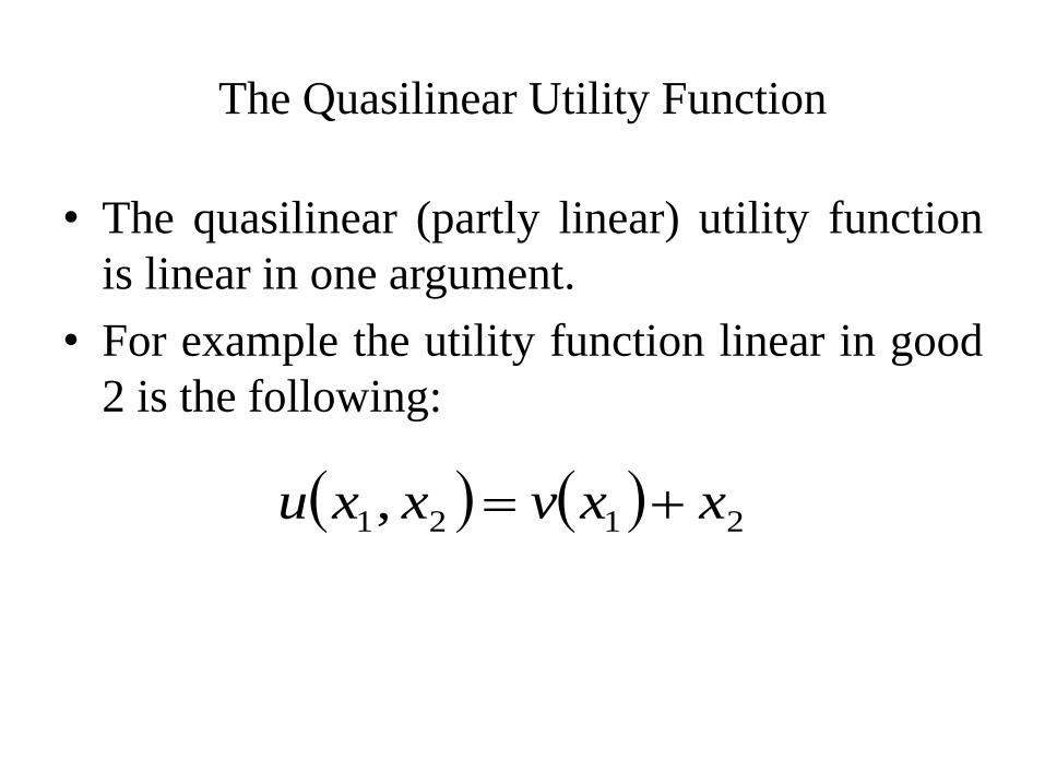
The Quasilinear Utility Function
• The quasilinear (partly linear) utility function
is linear in one argument.
• For example the utility function linear in good
2 is the following:
2121, xxvxxu

The Quasilinear Utility Function
• Specific examples of quasilinear utility would
be:
or
2121, xxxxu
2121 ln, xxxxu

The Homothetic Utility Function

The Homothetic Utility Function
The Homothetic Utility Function
• Slopes of indifference curves are constant along a ray through the origin.
• Assuming that preferences can be represented by a homothetic function is equivalent to assuming that they can be represented by a function that is homogenous of degree 1 because a utility function is unique up to a positive monotonic transformation.

The Marginal Utility

The Marginal Rate of Substitution
• Suppose that we increase the amount of good i;
how does the consumer have to change their
consumption of good j in order to keep utility
constant?
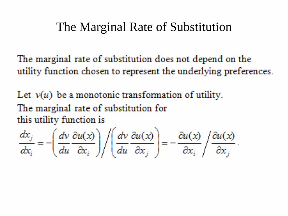
The Marginal Rate of Substitution

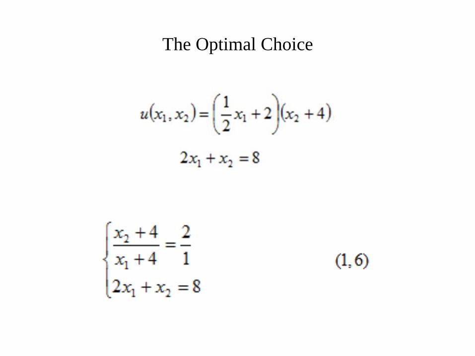
The Optimal Choice
• Consumers choose the most preferred bundle from their budget sets.
• The optimal choice of consumer is that bundle in the consumer’s budget
set that lies on the highest indifference curve.

The Optimal Choice
The Optimal Choice

The Optimal Choice
• Utility functions
• Budget line

The Optimal Choice

The Utility Maximization
• The problem of utility maximization can be written as:
• Consumers seek to maximize utility subject to their budget constraint.
• The consumption levels which solve the utility maximization problem are the Marshallian demand functions.

The Lagrange Method
• The method starts by defining an auxiliary
function known as the Lagrangean:
• The new variable l is called a Lagrange
multiplier since it is multiplied by constraint.

The Lagrange Method