MATHEMATICAL BACKGROUND AND ANALYSIS TECHNIQUES

1MATHEMATICAL BACKGROUND ANDANALYSIS TECHNIQUES

1.1 INTRODUCTION

This introductory chapter focuses on various mathematicaltechniques and solutions to practical problems encounteredin many of the following chapters. The discussions aredivided into three distinct topics: deterministic signal analy-sis involving linear systems and channels; statistical analysisinvolving probabilities, random variables, and random pro-cesses; miscellaneous topics involving windowing functions,mathematical solutions to commonly encountered problems,and tables of commonly used mathematical functions. Itis desired that this introductory material will provide thefoundation for modeling and finding practical design solu-tions to communication system performance specifications.Although this chapter contains a wealth of informationregarding a variety of topics, the contents may be viewedas reference material for specific topics as they are encoun-tered in the subsequent chapters.

This introductory section describes the commonly usedwaveform modulations characterized as amplitude modula-tion (AM), phase modulation (PM), and frequency modula-tion (FM) waveforms. These modulations result in thetransmission of the carrier- and data-modulated subcarriersthat are accompanied by negative frequency images. Thesetechniques are compared to the more efficient suppressedcarrier modulation that possesses attributes of the AM,PM, and FM modulations. This introduction concludeswith a discussion of real and analytic signals, the Hilberttransform, and demodulator heterodyning, or frequencymixing, to baseband.

Sections 1.2–1.4, deterministic signal analysis, transformin the context of a uniformly weighted pulse f(t) and its spec-trum F(f) and the duality between ideal time and frequencysampling that forms the basis of Shannon’s sampling theorem[1]. This section also discusses the discrete Fourier transform(DFT), the fast Fourier transform (FFT), the pipeline imple-mentation of the FFT, and applications involving waveformdetection, interpolation, and power spectrum estimation. Theconcept of paired echoes is discussed and used to analyze thesignal distortion resulting from a deterministic band-limitedchannel with amplitude and phase distortion. These sectionsconclude on the subject of autocorrelation and cross-correlation of real and complex deterministic functions; thecorresponding covariance functions are also examined.

Sections 1.5–1.10, statistical analysis, introduce the con-cept of random variables and various probability density func-tions (pdf) and cumulative distribution functions (cdf) forcontinuous and discrete random variables. Stochastic pro-cesses are then defined and the properties of ergodic and sta-tionary random processes are examined. The characteristicfunction is defined and examples, based on the summationof several underlying random variables, exhibit the trend inthe limiting behavior of the pdf and cdf functions toward thenormal distribution; thereby demonstrating the central limittheorem. Statistical analysis using distribution-free or nonpa-rametric techniques is introduced with a focus on order statis-tics. The random process involving narrowband whiteGaussian noise is characterized in terms of the noise spectraldensity at the input and output of an optimum detection filter.This is followed by the derivation of thematched filter and the

0002861001.3D 1 6/2/2017 7:47:47 AM

Digital Communications with Emphasis on Data Modems: Theory, Analysis, Design, Simulation, Testing, and Applications,First Edition. Richard W. Middlestead.© 2017 John Wiley & Sons, Inc. Published 2017 by John Wiley & Sons, Inc.Companion website: www.wiley.com/go/digitalcommunications

COPYRIG

HTED M

ATERIAL

equivalence between the matched filter and a correlationdetector is also established. The next subject discussedinvolves the likelihood ratio and log-likelihood ratio as theypertain to optimum signal detection. These topics are general-ized and expanded in Chapter 3 and form the basis for the opti-mum detection of the modulated waveforms discussed inChapters 4–9. Section 1.9 introduces the subject of parameterestimation which is revisited in Chapters 11 and 12 in the con-text of waveform acquisition and adaptive systems. The finaltopic in this section involves a discussion of modem configura-tions and the important topic of automatic repeat request(ARQ) to improve the reliability of message reception.

Sections 1.11–1.14, miscellaneous topics, include acharacterization of several window functions that are usedto improve the performance the FFT, decimation filtering,and signal parameter estimation. Section 1.12 provides anintroductory discussion of matrix and vector operations. InSection 1.13 several mathematical procedures and formulasare discussed that are useful in system analysis and simulationprogramming. These formulas involve prime factorization ofan integer and determination of the greatest common factor(GCF) and least common multiple (LCM) of two integers,Newton’s approximation method for finding the roots ofa transcendental function, and the definition of thestandard deviation of a sampled population. This chapterconcludes with a list of frequently used mathematical formu-las involving infinite and finite summations, the binomialexpansion theorem, trigonometric identities, differentiationand integration rules, inequalities, and other miscellaneousrelationships.

Many of the examples and case studies in the followingchapters involve systems operating in a specific frequencyband that is dictated by a number of factors, including, thesystem objectives and requirements, the communicationrange equation, the channel characteristics, and the result-ing link budget. The system objectives and requirementsoften dictate the frequency band that, in turn, identifies thechannel characteristics. Table 1.1 identifies the frequency

band designations with the corresponding range of frequen-cies. The designations low frequency (LF), medium fre-quency (MF), and high frequency (HF) refer to low,medium, and high frequencies and the prefixes E, V, U,and S correspond to extremely, vary, ultra, and super.

1.1.1 Waveform Modulation Descriptions

This section characterizes signal waveforms comprised ofbaseband information modulated on an arbitrary carrier fre-quency, denoted as fc Hz. The baseband information is char-acterized as having a lowpass bandwidth of B Hz and, intypical applications, fc >> B. In many communication systemapplications, the carrier frequency facilitates the transmissionbetween the transmitter and receiver terminals and can beremoved without effecting the information. When the carrierfrequency is removed from the received signal the signal pro-cessing sampling requirements are dependent only on thebandwidth B.

The signal modulations described in Sections 1.1.1.1through 1.1.1.4 are amplitude, phase, frequency, and sup-pressed carrier modulations. The amplitude, phase, and fre-quency modulations are often applied to the transmissionof analog information; however, they are also used in variousapplications involving digital data transmission. For exam-ple, these modulations, to varying degrees, are the underlyingwaveforms used in the U.S. Air Force Satellite ControlNetwork (AFSCN) involving satellite uplink and downlinkcontrol, status, and ranging.

In describing the demodulator processing of the receivedwaveforms, the information, following removal of the carrierfrequency, is associated with in-phase and quadphase (I/Q)baseband channels or rails. Although these I/Q channelsare described as containing quadrature real signals, theyare characterized as complex signals with real and imaginaryparts. This complex signal description is referred to as com-plex envelope or analytic signal representations and is dis-cussed in Section 1.1.1.5. Suppressed carrier modulationand the analytic signal representation emphasize quadraturedata modulation that leads to a discussion of the Hilberttransform in Section 1.1.1.6. Section 1.1.1.7 discusses con-ventional heterodyning of the received signal to basebandfollowed by data demodulation.

1.1.1.1 Amplitude Modulation Conventional amplitudemodulation (AM) is characterized as

s t =A 1 +mIm t sin ωmt sin ωct (1.1)

where A is the peak carrier voltage, mI > 0 is the modulationindex, m(t) is the information modulation function, ωm is themodulation angular frequency, and ωc is the AM carrierangular frequency. Upon multiplying (1.1) through by sin

TABLE 1.1 Frequency Band Designations

Designation FrequencyLetterDesignation

Frequency(GHz)

ELF 3–30 Hz L 1–2SLF 30–300 Hz S 2–4ULF 0.3–3 kHz C 4–8VLF 3–30 kHz X 8–12LF 30–300 kHz Ku 12–18MF 0.3–3 MHz K 18–27HF 3–30 MHz Ka 27–40VHF 30–300 MHz V 40–75UHF 0.3–3 GHz W 75–110SHF 3–30 GHz mm (millimeter) 110–300EHF 30–300 GHz

0002861001.3D 2 6/2/2017 7:47:48 AM

2 MATHEMATICAL BACKGROUND AND ANALYSIS TECHNIQUES

(ωct) and applying elementary trigonometric identities, theAM-modulated signal is expressed as

s t =Asin ωct +AmI

2m t cos ωc−ωm t

−AmI

2m t cos ωc +ωm t

(1.2)

Therefore, s(t) represents the conventional double side-band (DSB) AM waveform with the upper and lower side-bands at ωc ±ωm equally spaced about the carrier at ωc.With the information modulation function m(t) normalizedto unit power, the power in each sideband is mIPS/4 wherePS is the power in the carrier frequency fc.

1.1.1.2 Phase Modulation Conventional phase modula-tion (PM) is characterized as

s t =Asin ωct +φ t (1.3)

where A is the peak carrier voltage, ωc is the carrier angularfrequency, and φ(t) is an arbitrary phase modulation functioncontaining the information. The commonly used phase func-tion is expressed as

φ t =ϕsin ωmt (1.4)

where ϕ is the peak phase deviation. Substituting (1.4) into(1.3), the phase-modulated signal is expressed as

s t =A sin ωct +ϕsin ωmt (1.5)

and, upon applying elementary trigonometric identities, (1.5)yields

s t =Asin ωct cos ϕsin ωmt +Acos ωct sin ϕsin ωmt

(1.6)

The trigonometric functions involving sinusoidal argu-ments can be expanded in terms of Bessel functions [2]and (1.6) simplifies to

s t =AJ0 ϕ sin ωct +A∞

n = 1

Jn ϕ sin ωc + nωm t

+ −1 nJn ϕ sin ωc−nωm t

(1.7)

Equation (1.7) is characterized by the carrier frequencywith peak amplitude AJ0(ϕ) and upper and lower sidebandpairs at ωc ± nωm with peak amplitudes AJn(ϕ). For smallarguments the Bessel functions reduce to the approximationsJ0 ϕ 1,J1 ϕ ϕ 2 with Jn ϕ 0 n> 1 and (1.7)reduces to

s t Asin ωct +Aϕ

2sin ωc +ωm t −

Aϕ

2sin ωc−ωm t

small ϕ(1.8)

Under these small argument approximations, the similari-ties between (1.8) and (1.2) are apparent.

1.1.1.3 FrequencyModulation The frequency-modulated(FM) waveform is described as

s t =Asin ωct +Δffm

sin ωmt (1.9)

where A is the peak carrier voltage, ωc is the carrier angularfrequency, Δf is the peak frequency deviation of the modula-tion frequency fm, and ωm is the modulation angular fre-quency. The ratio Δf/fm is the frequency modulation index.Noting the similarities between (1.9) and (1.5), the expres-sion for the frequency-modulated waveform is expressed,in terms of the Bessel functions, as

s t =AJ0Δffm

sin ωct +A∞

n = 1

JnΔffm

sin ωc + nωm t

+ −1 nJnΔffm

sin ωc−nωm t

(1.10)

with the corresponding small argument approximation for theBessel function expressed as

s t Asin ωct +AΔf2fm

sin ωc +ωm t −AΔf2fm

sin ωc−ωm t

smallΔffm

(1.11)

The similarities between (1.11), (1.8), and (1.2) are apparent.

1.1.1.4 Suppressed Carrier Modulation A commonlyused form of modulation is suppressed carrier modulationexpressed as

s t =Am t sin ωct +φ t (1.12)

In this case, when the carrier is mixed to baseband, infor-mation modulation functionm(t) does not have a direct current(DC) spectral component involving δ(ω). So, upon multiplica-tion by the carrier, there is no residual carrier component ωc inthe received baseband signal. Because the carrier is suppressedit is not available at the receiver/demodulator to provide acoherent reference, so special considerations must be given

0002861001.3D 3 6/2/2017 7:47:49 AM

INTRODUCTION 3

to the carrier recovery and subsequent data demodulation.Suppressed carrier-modulated waveforms are efficient, inthat, all of the transmitted power is devoted to the information.Suppressed carrier modulation and the various methods ofcarrier recovery are the central focus of the digital communi-cation waveforms discussed in the following chapters.

1.1.1.5 Real and Analytic Signals The earlier modula-tion waveforms are described mathematically as real wave-forms that can be transmitted over real or physicalchannels. The general description of the suppressed carrierwaveform, described in (1.12), can be expressed in termsof in-phase and quadrature modulation functions mc(t) andms(t) as

s t =mc t cos ωct −ms t sin ωct (1.13)

The quadrature modulation functions are expressed as

mc t =Adcm t cos φ t (1.14)

and

ms t =Adsm t sin φ t (1.15)

With PM the data {dc, ds} may be contained in a phasefunction φd(t), m(t) is a unit energy symbol shaping functionthat provides for spectral control relative to the commonlyused rect(t/T) function, and A represents the peak carriervoltage on each rail. With quadrature modulations, uniquesymbol shaping functions, mc(t) and ms(t), may be appliedto each rail; for example, unbalanced quadrature modulationsinvolve different data rates on each quadrature rail. Withquadrature amplitude modulation (QAM) the data isdescribed in terms of the multilevel quadrature amplitudes{αc, αs} that are used in place of {dc, ds} in (1.14) and (1.15).

Equation (1.13) can also be expressed in terms of the realpart of a complex function as

s t =Re s t ejωct (1.16)

where

s t =mc t + jms t (1.17)

The function s t is referred to as the complex envelope oranalytic representation of the baseband signal and plays afundamental role in the data demodulation, in that, it containsall of the information necessary to optimally recover thetransmitted information. Equation (1.17) applies to receiversthat use linear frequency translation to baseband. Linear fre-quency translation is typical of heterodyne receivers usingintermediate frequency (IF) stages. This is a significant resultbecause the system performance can be evaluated using the

analytic signal without regard to the carrier frequency [3];this is particularly important in computer performancesimulations.

Evaluation of the real part of the signal expressed in (1.16)is performed using the complex identity No. 4 inSection 1.14.6 with the result

s t =12

s t ejωct + s t ∗e− jωct (1.18)

A note of caution is in order, in that, the received signalpower based on the analytic signal is twice that of the powerin the carrier. This results because the analytic signal does notaccount for the factor of 1/2 when mixing or heterodyningwith a locally generated carrier frequency and is directlyrelated the factor of 1/2 in (1.18). The signal descriptionsexpressed in (1.12) through (1.18) are used to describe thenarrowband signal characteristics used throughout much ofthis book.

1.1.1.6 Hilbert Transform and Analytic Signals TheHilbert transform of the real s(t) is defined as

s t ≜1π

∞

−∞

s τ

t−τdτ = s t ∗ 1

πt(1.19)

The second expression in (1.19) represents the convolu-tion of s(t) with a filter with impulse response h t = 1 πtwhere h(t) represents the response to a Hilbert filter with fre-quency response H(ω) characterized as

h t H ω

=− jsign ω ω > 0

0 o w

(1.20)

The Hilbert transform of s(t) results in a spectrum that iszero for all negative frequencies with positive frequenciesrepresenting a complex spectrum associated with the realand imaginary parts of an analytic function. Applying(1.20) to the signal spectrum S ω s t results in the spec-trum of the Hilbert transformed signal

S ω =

jS ω ω< 0

0 ω= 0

− jS ω ω> 0

(1.21)

Applying (1.21) to the spectrum S(ω) of (1.12) or (1.13),the bandwidth B of m(t) must satisfy the condition B << fc.In this case, the inverse Fourier transform of the spectrumS ω yields the Hilbert filter output s t given by

0002861001.3D 4 6/2/2017 7:47:49 AM


s t = TH Am t sin ωct +ϕ t =Am t sin ωct +ϕ t −π 2

= −Am t cos ωct +ϕ t

(1.22)

where TH[s(t)] represents the Hilbert transform of s(t).The function s t expressed by (1.22) is orthogonal to s(t)

and, if the carrier frequency were removed following theHilbert transform, the result would be identical to theimaginary part of the analytic signal expressed by (1.17).The processing is depicted in Figure 1.1.

1.1.1.7 Conventional and Complex Heterodyning Con-ventional heterodyning is depicted in Figure 1.2. The zonalfilters are ideal low-pass filters with frequency responsegiven by

H f = rect f −fc2

zonal lowpass filter (1.23)

These filters remove the 2ωc term that results from themixing operation and, for s(t) as expressed by (1.13), thequadrature outputs are given by

sc t =A

2mc t cos ϕ t −ms t sin ϕ t (1.24)

and

ss t =A

2mc t sin ϕ t +ms t cos ϕ t (1.25)

With ideal phase tracking the phase term ϕ(t) is zeroresulting in the quadrature modulation functions mc(t) andms(t) in the respective low-pass channels.

1.2 THE FOURIER TRANSFORM ANDFOURIER SERIES

The Fourier transform is so ubiquitous in the technical liter-ature [4–6], and its application are so widely used that itseems unnecessary to dwell at any length on the subject.However, a brief description is in order to aid in the under-standing of the parameters used in the applications discussedin the following chapters.

The Fourier transform F(f) of f(t) is defined over the inter-val t ≤ ∞ and, if f(t) is absolutely integrable, that is, if

∞

−∞

f t dt < ∞ (1.26)

then F(f) exists, furthermore, the inverse Fourier transformof F(f) results in f(t). In most applications* of practical inter-est, f(t) satisfies (1.26) leading to the Fourier transform pairf t F f defined as

F f =

∞

−∞

f t e− j2πftdt f t =

∞

−∞

F f ej2πftdf (1.27)

In general, f(t) is real and the Fourier transform F(f) iscomplex and Parseval’s theorem relates the signal energyin the time and frequency domains as

∞

−∞

f t 2dt =

∞

−∞

F f 2df (1.28)

The Fourier series representation of a periodic function isclosely related to the Fourier transform; however, it is basedon orthogonal expansions of sinusoidal functions at discretefrequencies. For example, if the function of interest is peri-odic, such that, f(t) = f(t – iTo) with period To and is finiteand single valued over the period, then f(t) can be representedby the Fourier series

f t =∞

n= −∞Cne

jnωot (1.29)

where ωo = 2π/To and Cn is the n-th Fourier coefficientgiven by

s(t) s(t)

s(t)˘Hilbertfilter

FIGURE 1.1 Hilbert transform of carrier-modulated signal s(t)B fc 1 .

Ss(t)

Sc(t)

s(t)

cos(ωct)

Zonalfilter

–sin(ωct)

Zonalfilter

FIGURE 1.2 Heterodyning of carrier-modulated signal s(t)B fc 1 .

*For special cases refer to Papoulis (Reference 7, Chapter 2).

0002861001.3D 5 6/2/2017 7:47:50 AM

THE FOURIER TRANSFORM AND FOURIER SERIES 5

Cn =1To

To 2

−To 2

f t e− jnωotdt (1.30)

Equation (1.29) is an interesting relationship, in that, f(t)can be described over the time interval To by an infinite setof frequency-domain coefficient Cn; however, because f(t)is contiguously replicated over all time, that is, it is periodic,the spectrum of f(t) is completely defined by the coefficientsCn. Unlike the Fourier transform, the spectrum of (1.29) is notcontinuous in frequency but is zero except at discrete fre-quencies occurring at multiples of nωo. This is seen by takingthe Fourier transform of (1.29) and, using (1.27), the result isexpressed as

F f =∞

n= −∞Cn

∞

−∞

e− j2π f −nfo tdt

=∞

n= −∞Cnδ f −nfo

(1.31)

where δ f −nfo is the Fourier Transform* of ejnωoT .Equation (1.31) is applied in Chapter 2 in the discussion ofsampling theory and in Chapter 11 in the context of signalacquisition.

Alternate forms of (1.29) that emphasize the series expan-sion in terms of harmonics of trigonometric functions aregiven in (1.32) and (1.33) when f(t) is a real-valued function.This is important because when f(t) is real the complex coef-ficients Cn and C−n form a complex conjugate pair such thatC−n =C∗

n which simplifies the evaluation of f(t). For example,using the complex notations Cn = αn + jβn and C∗

n = αn− jβn,the function f(t) is evaluated as

f t =Co + 2∞

n= 1

αn cos nωot −βn sin nωot (1.32)

this simplifies to

f t =Co + 2∞

n= 1

Cn cos nωot +ϕn (1.33)

where Cn = α2 + β2 and ϕn = arctan β α .An important consideration in spectrum analysis is the

determination of signal spectrums involving random datasequences, referred to as stochastic processes [8]. A stochas-tic process does not have a unique spectrum; however, thepower spectral density (PSD) is defined as the Fouriertransform of the autocorrelation response. Oppenheim and

Schafer [9] discuss methods of estimating the PSD of areal finite-length (N) sampled sequence by averagingperiodograms, defined as

IN ω =1N

F ω 2 (1.34)

where F(ω) is the Fourier transform of the sampled sequence.This method is accredited to Bartlett [10] and is used in theevaluation of the PSD in the following chapters. For a fixedlength (L) of random data, the number of periodograms (K)that can be averaged is K = L/N. As K increases the varianceof the spectral estimate approaches zero and as N increasesthe resolution of the spectrum increases, so there is a trade-off between the selection of K and N. To resolve narrowbandspectral features that occur, for example, with nonlinearfrequency shift keying (FSK)-modulated waveforms, it isimportant to use large values of N. Fortunately, many ofthe spectrum analyses presented in the following chaptersare not constrained by L so K and N are chosen to providea low estimation bias, that is, low variance, and high spectralresolution. Windowing† the periodograms will also reducethe estimation bias at the expense of decreasing the spectralresolution.

1.2.1 The Transform Pair rect(t/T) Tsinc(fT)

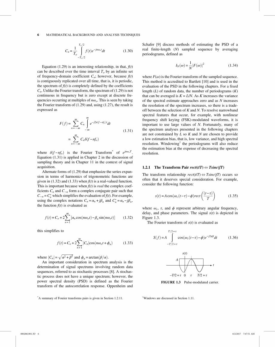
The transform relationship rect(t/T) Tsinc(fT) occurs sooften that it deserves special consideration. For example,consider the following function:

s t =Acos ωc t−τ −ϕ rectt−τ

T(1.35)

where ωc, τ, and ϕ represent arbitrary angular frequency,delay, and phase parameters. The signal s(t) is depicted inFigure 1.3.

The Fourier transform of s(t) is evaluated as

S f =A

T 2 + τ

−T 2 + τ

cos ωc t−τ −ϕ e− j2πftdt (1.36)

T/2 + τ–T/2 + τ τ

A

0

t

s(t)

FIGURE 1.3 Pulse-modulated carrier.

*A summary of Fourier transforms pairs is given in Section 1.2.11. †Windows are discussed in Section 1.11.

0002861001.3D 6 6/2/2017 7:47:51 AM


Expressing the cosine function in terms of complexexponential functions and performing some simplificationsresults in the expression

S f =A

2e− j 2πf τ +ϕ

τ + T 2

τ−T 2

e− j2π f − fc tdt

+ e− j 2πf τ−ϕτ + T 2

τ−T 2

e− j2π f + fc tdt

(1.37)

Evaluation of the integrals in (1.37) appears so often that itis useful to generalize the solutions as follows:

Consider the integral

I y =

x2

x1

e− j y ± y xdx

=e− j y ± y x2 −e− j y ± y x1

− j y± y

(1.38)

The general solution involves multiplying the last equalityin (1.38) by the factors e− j y ± y x2 + x1 2 and ej y ± y x2 + x1 2,having a product of one, where x2 + x1 2 is the averageof the integration limits. Distributing the second factor overthe numerator of (1.38) and then simplifying yields the result

I y = x2−x1 e− j y ± y x2 + x1 2 sin y ± y x2−x1 2y ± y x2−x1 2

(1.39)

Applying (1.39) to (1.37) and simplifying gives thedesired result

S f =AT

2e− j 2πf τ +ϕ sinc f − fc T + e− j 2πf τ−ϕ sinc f + fc T

(1.40)

When fc 1 T , the positive and negative frequencyspectrums do not influence one another and, in this case,the positive frequency spectrum is defined as

S+ f =AT

2sinc f − fc T fc

1T

(1.41)

On the other hand, when the carrier frequency and phaseare zero, (1.40) simplifies to the baseband spectrum, evalu-ated as

Sbb f =ATe− j2πf τsinc fT fc = 0, ϕ= 0 (1.42)

Using (1.42), the baseband Fourier transform pair, corre-sponding to of (1.35) with fc = 0, is established as

rectt−τ

TTe− j2πf τsinc fT t−τ ≤

T

2(1.43)

and, with τ = 0,

rectt

TTsinc fT t ≤

T

2(1.44)

1.2.2 The sinc(x) Function

The sinc(x) function is defined as

sinc x =sin πx

πx(1.45)

and is depicted in Figure 1.4. When x is expressed as the nor-malized frequency variable x = fT then (1.45), when scaled byT, is the frequency spectrum of the unit amplitude pulse rect(t/T) of duration T seconds such that t ≤ |T/2|. This function issymmetrical in x and the maximum value of the first sidelobeoccurs at x=1.431with a level of 10log(sinc2(x)) =−13.26 dB;the peak sidelobe levels decrease in proportion to 1/|x|. Thenoise bandwidth of a filter function H(f) is defined as

Bn ≜

∞

−∞H f 2df

H fo2 (1.46)

where fo is the filter frequency corresponding to the maxi-mum response. When a receiver filter is described asH(f) = sinc(fT) the receiver low-pass noise bandwidth is eval-uated as Bn = 1/T where T is the duration of the filter impulseresponse.

x0 1 2 3 4 5 6 7 8 9

sinc

(x)

–0.4

–0.2

0.0

0.2

0.4

0.6

0.8

1.0

FIGURE 1.4 The sinc(x) function.

0002861001.3D 7 6/2/2017 7:47:51 AM


It is sometimes useful to evaluate the area of the sinc(x)function and, while there is no closed form solutions, thesolution can be evaluated in terms of the sine-integralSi(x)

* as

z

0sinc x dx=

z

0

sin πx

πxdx=

1π

π z

0

sin λ

λdλ

=1πSi πz

(1.47)

where the sine-integral is defined as the integral of sin(λ)/λ.Equation (1.47) is shown in Figure 1.5. The limit of Si(πz) as|z| ∞ is† π sign(1,z)/2 so the corresponding limit of (1.47)is 0.5sgn(z).

A useful parameter, often used as a benchmark forcomparing spectral efficiencies, is the area under sinc2(x)as a function of x. The area is evaluated in terms of thesine-integral as

z

0sinc2 x dx=

z

0

sin2 πx

πx 2 dx

=1π

Si 2πz −sin2 2πz

2πz

(1.48)

Equation (1.48) is plotted in Figure 1.6 as a percent of thetotal area and it is seen that the spectral containment of 99%is in excess of 18 spectral sidelobes, that is, x = fT = 18. Inthe following chapters, spectral efficient waveforms areexamined with 99% containment within 2 or 3 sidelobes,so the sinc(x) function does not represent a spectrally efficientwaveform modulation.

1.2.3 The Fourier Transform Pair

nδ t−nT ωo n

δ ω−nωo

The evaluation of this Fourier transform pair is fundamentalto Nyquist sampling theory and is demonstrated inSection 2.3 in the evaluation of discrete-time sampling. In thiscase, the function f(t) is an infinite repetition of equally spaceddelta functions δ(t) with intervals T seconds as expressed by

f t =∞

n= −∞δ t−nT (1.49)

The challenge is to show that the Fourier transform of(1.49) is equal to an infinite repetition of equally spacedand weighted frequency domain delta functions expressed as

F ω =ωo

∞

n= −∞δ ω−nωo (1.50)

with weighting ωo and frequency intervals ωo = 2π T . Directapplication of the Fourier transform to (1.49) leads to the

spectrumne− jnωT but this does not demonstrate the equal-

ity in (1.50). Similarly, evaluation of the inverse Fouriertransform of (1.50) results in the time-domain expression

g t =1T

∞

n = −∞ejnωot (1.51)

So, by showing that g t = f t , the transform pair between(1.49) and (1.50) will be established. Consider gN(t) to be afinite summation of terms in (1.51) given by

gN t =1T

N

n= −N

ejnωot

=sin 2N + 1 ωot 2

T sin ωot 2

(1.52)

x0 2 4 6 8 10 12 14 16 18

Inte

gral

sin

c2 (x)

(%

of

tota

l)

0

20

40

60

80

100

FIGURE 1.6 Integral of sinc2(x) function.

x0 1 2 3 4 5 6 7 8 9

Inte

gral

sin

c(x)

0.00

0.25

0.50

0.75

FIGURE 1.5 Integral of sinc(x).

*The arguments x and z may be complex; however, the following analysisuses only real arguments.†The sign(a, x) function is defined in Section 1.14.7.

0002861001.3D 8 6/2/2017 7:47:52 AM


The second equality in (1.52) can be shown usingthe finite series identity No. 12, Section 1.14.1. Equation(1.52) is referred to by Papoulis [7] as the Fourier-serieskernel and appears in a number of applications involvingthe Fourier transform.

The function gN(t) is plotted in Figure 1.7 for N = 8. Theabscissa is time normalized by the pulse repetition intervalT = 1 fo such that, gN t = gN t−nT , and there are a totalof 2N + 1 peaks of which three are shown in the figure. Fur-thermore, there are eight time sidelobes between t/T = 0 and0.5 with the first nulls from the peak value at t/T = 0 occurringat ±T 2N + 1 ; the peak values are 2N + 1 T = 17 T inthis example.

The maximum values of 2N + 1, occurring at t T = n, aredetermined by applying L’Hospital’s rule to (1.52), which isrewritten as

gN t = 2N + 1sin 2N + 1 ωot 2T 2N + 1 sin ωot 2

2N + 1sin 2N + 1 ωot 2T 2N + 1 ωot 2

(1.53)

The approximation in (1.53) is obtained by noting thatas N increases the rate of the sinusoidal variations in thenumerator term increases with a frequency of 2N + 1 fo Hzwhile the rate of sinusoidal variation in the denominatorremains unchanged. Therefore, in the vicinity of t T = n,sin ωot 2 ωot 2 and (1.53) reduces to a sin(x)/x functionwith x = 2N + 1 ωot 2 and a peak amplitude (2N + 1). Theproof of the transform pair is completed by showing thatf(t) = g(t). Referring to (1.51) g(t) is expressed as

g t = limN ∞

gN t (1.54)

From (1.53) as N approaches infinity the sin(x)/x sidelobenulls converge to t/T = n, the peak values become infinite,and the corresponding area over the interval |t/T| = n ± 1/2approaches unity. Therefore, g(t) resembles a periodic seriesof delta functions resulting in the equality

g t = limN ∞

gN t =∞

n = −∞δ t−nT

= f t

(1.55)

thus completing the proof that (1.49) and (1.50) correspond toa Fourier transform pair. Papoulis (Reference 7, pp. 50–52)provides a more eloquent proof that the limiting form ofgN(t) is indeed an infinite sequence of delta functions.

1.2.4 The Discrete Fourier Transform

The DFT pair relating the discrete-time function f(mΔt) ≡f(m) and discrete-frequency function F(nΔf) ≡ F(n) is de-noted as f m F n where

F n =ΔtM−1

m = 0

f m e− j2πnΔfmΔt f m =ΔfN−1

n = 0

F n ej2πnΔfmΔt

DFT

(1.56)

With the DFT the number of time and frequency samplescan be chosen independently. This is advantageous when pre-paring presentation material or examining fine spectral ortemporal details, as might be useful when debugging simula-tion programs, by the independent selection of the integers mand n.

1.2.5 The Fast Fourier Transform

As discussed in the preceding section, the DFT pair, relatingthe discrete-time function f(mΔt) ≡ f(m) and the discrete-frequency function F(nΔf) ≡ F(n), is denoted as f m

F n where f(m) and F(n) are characterized by the expres-sions for the DFT. The FFT [11–17], is a special case corre-sponding to m and n being equal to N as described in theremainder of this section. In these relationships N is the num-ber of time samples and is defined as the power of a fixedradix-r FFT or as the powers of a mixed radix-rj FFT.

*

The fixed radix-2 FFT, with r = 2 and N = 2i, results in themost processing efficient implementation.

Normalized time (t/T)–1.5 –1.0 –0.5 0.0 0.5 1.0 1.5

Am

plit

ude

(A)

volt

s

0

5

10

15

20

… …

(2N + 1)/T

T/(2N + 1)

FIGURE 1.7 The Fourier-series kernel gN(t) (N = 8).

*Mixed radix FFTs provide an efficient method of computing the Fouriertransform when the number of samples is not a power of r. In general,N = r1 i1 r2 i2… and the radices of the FFT are determined as the prime factorsof N. For example, N = 31 = 1∗31 requires a single radix = 31 FFT, N = 32 =2∗2∗2∗2∗2 requires a radix-2 FFT, and N = 33 = 3∗11 requires a radix-3 anda radix-11 FFT.

0002861001.3D 9 6/2/2017 7:47:53 AM


Defining the time window of the FFT as Tw results inan implicit periodicity of f(t) such that f(t) = f(t ± kTw)and Δt = Tw/N. The sampling frequency is defined asfs = 1 Δt =N Tw and, based on Shannon’s sampling theo-rem, the periodicity does not pose a practical problem aslong as the signal bandwidth is completely contained inthe interval |B| ≤ fs/2 = N/(2Tw). Since the FFT results inan equal number of time and frequency domain samples, thatis,Δf = fs/N andΔt = Tw/N, it follows thatΔfΔt = fs Tw/N

2 = 1/N. Normalizing the expression of the time function, f(m), in(1.56), that is, multiplying the inverse DFT (IDFT) by Δtrequires dividing the expression for F(n) by Δt. Upon substi-tuting these results into (1.56), the FFT transform pairsbecome

F n =N−1

m= 0

f m e− j2πnm N f m =1N

N−1

n = 0

F n ej2πnm N

FFT

(1.57)

The time and frequency domain sampling characteristicsof the FFT are shown in Figure 1.8. This depiction focuseson a communication system example, in that, the time sam-ples over the FFT window interval Tw are subdivided intoNsym symbol intervals of duration T seconds with Ns sam-ples/symbol.

Typically the bandwidth of the modulated waveform istaken to be the reciprocal of the symbol duration, that is, 1/THz; however, the receiver bandwidth required for low sym-bol distortion is typically several times greater than 1/Tdepending upon the type of modulation. Referring toFigure 1.8 the sampling frequency is fs = 1/Δt, the samplinginterval is Δt = T/Ns, the size of the FFT is Nfft = NsNsym, andthe frequency sampling increment is Δf = fs/Nfft. Upon usingthese relationships, the frequency resolution, or frequencysamples per symbol bandwidth B = 1/T, is found to be

B

Δf=Nsym determines frequency resolution (1.58)

and the number of spectral sidelobes* or symbol bandwidthsover the sampling frequency range is

fsB=Ns determines spectral sidelobes (1.59)

Therefore, to increase the resolution of the sampled signalspectrum, the number of symbols must be increased and this

is comparable to increasing Tw. On the other hand, to increasethe number of signal sidelobes contained in the frequencyspectrum the number of samples per symbol must beincreased and this is comparable to decreasing Δt. Both ofthese conditions require increasing the size (N) of the FFT.However, for a given size, the FFT does not allow independ-ent selection of the frequency and time resolution asdetermined, respectively, by (1.58) and (1.59). This can beaccomplished by using the DFT as discussed inSection 1.2.4. Since the spectrum samples in the range 0 ≤f < fs/2 represent the positive frequency signal spectrumand those over the range fs/2 ≤ f < fs represent the negativefrequency signal spectrum, the range of signal sidelobes ofinterest is ±fs/(2B) = ±Ns/2. As a practical matter, if the signalcarrier frequency is not zero then the sampling frequencymust be increased to maintain the signal sidelobes aliasingcriterion. The sampling frequency selection is discussed inChapter 11 in the context of signal acquisition when thereceived signal frequency is estimated based on locallyknown conditions.

The following implementation of the FFT is based on theCooley and Tukey [18] decimation-in-time algorithm asdescribed by Brigham and Morrow [19] and Brigham [20].Although (1.57) characterizes the FFT transform pairs, thereal innovation leading to the fast transformation is realizedby the efficient algorithms used to execute the transforma-tion. Considering the radix-2 FFT with N = 2n, this involvesdefining the constant

W ≜ e− j2π N (1.60)

and recognizing that

F n =ΔtN−1

m= 0

f m Wnm (1.61)

Equation (1.61) can be expressed in matrix form, usingN = 4 for simplicity, as

Nsym : symbols / window (Tw)Ns : samples / symbol (T)

…

0 3T2T

f(mΔt)

ΔtTw =

NsymT

t…

(a)

Tf

(b)

…

F(nΔf )

Δffs / 2 fs =

Nfft Δf0 1/T

Ns : bandwidths / frequency ( fs)Nsym : samples / bandwidth (B)

Bandlimited sampled spectrum( f = nΔf )

Time sampled waveform(t = mΔt)

FIGURE 1.8 FFT time and frequency domain sampling.

*These results are based on the underlying rect(t/T) window and the sinc(fT)frequency function that includes the principal lobe and the positive and neg-ative spectral side lobes.

0002861001.3D 10 6/2/2017 7:47:53 AM


F 0

F 1

F 2

F 3

=Δt

W0 W0 W0 W0

W0 W1 W2 W3

W0 W2 W4 W6

W0 W3 W6 W9

f 0

f 1

f 2

f 3

(1.62)

Recognizing that W0 = 1 and the exponent nm is modulo(N), upon factoring the matrix in (1.62) into the product oftwo submatrices (in general the product of log2N subma-trices) leads to the implementation involving the minimumnumber of computations expressed as

F 0

F 2

F 1

F 3

=Δt

1 W0 0 0

1 W2 0 0

0 0 1 W1

0 0 1 W3

1 0 W0 0

0 1 0 W2

1 0 W2 0

0 1 0 W2

f 0

f 1

f 2

f 3

(1.63)

The simplifications result in the outputs F(2) and F(1)being scrambled and the unscrambling to the natural-numberordering simply involves reversing the binary numberequivalents, that is, with F (1) = F(2) and F (2) = F (1); there-fore, the unscrambling is accomplished as F(1) = F (01) =F (2) = F (10) and F (2) = F (10) = F (1) = F (01). Theradix-2 with N = 4 FFT, described by (1.63), is implementedas shown in the diagram of Figure 1.9.

The inverse FFT (IFFT) is implemented by changing thesign of the exponent ofW in (1.60), interchanging the roles ofF(n) and f(m), as described earlier, and replacing Δt by Δf.

Recognizing that ΔtΔf = 1/N, it is a common practice notto weight the FFT but to weight the IFFT by 1/N as indicatedin (1.57). The number of complex multiplication is deter-mined from (1.63) by recognizing that W2 = −W0 and notcounting previous products like W0f(2) from row 1 andW2f(2) = −W0f(0) from row 3 in the first matrix multiplicationon the rhs of (1.63). For the commonly used radix-2 FFT, thenumber of complex multiplications is (N/2)log2(N) and thenumber of complex additions is Nlog2(N). By comparison,the number of complex multiplications and additions in thedirect Fourier transform are N2 and N(N − 1), respectively.These computational advantages are enormous for even mod-est transform sizes.

1.2.5.1 The Pipeline FFT The FFT algorithm discussedin the preceding section involves decimation-in-time proces-sing and requires collecting an entire block of time-sampleddata prior to performing the Fourier transform. In contrast,the pipeline FFT [21] processes the sampled data sequentiallyand outputs a complete Fourier transform of the stored data ateach sample. The implementation of a radix-2, N = 8-pointpipeline FFT is shown in Figure 1.10. The pipeline FFTinherently scrambles the outputs F (n) and the unscrambledoutputs are not shown in the figure; the unscrambling isaccomplished by simply reversing the order of the binaryrepresentation of the output locations, n, as described inthe preceding section.

In general, the number of complex multiplications for acomplete transform is (N/2)(N − 1). In Chapter 11 the pipelineFFT is applied in the acquisition of a waveform where a

F′(3)

F′(2)

F′(1)

F′(0)

F(3)

F(2)

F(1)

F(0)

W 1

W 0

W 2

W 2

W 2

W 3

W 0

W 0

1

1

11

1

1

11

f(2)

f(3)

f(1)

f(0)

Ts

Ts

Ts Unscramble

Sampleddata

FIGURE 1.9 Radix-2, N = 4-point FFT implementation tree diagram.

0002861001.3D 11 6/2/2017 7:47:54 AM


complete N-point FFT output is not required at every sample.For example, if the complete N-point FFT is only required atsample intervals of NsTs, the number of complex multiplica-tions can be significantly reduced (see Problem 10). Thepipeline FFT can be used to interpolate between thefundamental frequency cells by appending zeros to the datasamples and appropriately increasing the size of the FFT;it can also be used with data samples requiring mixed radixprocessing. The pipeline FFT is applicable to radar and sonarsignal detection processing [21] using a variety of spectralshaping windows; however, the intrinsic rect(t/T) FFT win-dow is nearly matched for the detection of orthogonallyspaced M-ary FSK modulated frequency tones.

1.2.6 The FFT as a Detection Filter

The pipeline Fourier transform is made up of a cascade oftransversal filter building blocks shown in Figure 1.10. Thetransfer function of this building block is

Ti s =eo s

ei s

=Wi + e−skiTs

(1.64)

The overall transfer function from the input to a particularoutput is evaluated as

Sampleddata

+

+

+

+

+

+

+

+

+

+

+

+

+

+

+

–

–

–

–

–

–

–

+

+

+

+

+

+

F′(0)

F′(1)

F′(2)

F′(3)

F′(4)

F′(5)

F′(7)

F′(6)

f(m)

W3

W1

W2

W2

W0

W0

W0 Ts

Ts

Ts

Ts

2Ts

2Ts

4Ts

FIGURE 1.10 Radix-2, N = 8-point pipeline FFT implementation tree diagram.

0002861001.3D 12 6/2/2017 7:47:54 AM


Tℓ s =eℓ s

ei s

=k

i= 1

Wℓ, i + e−skiTs

(1.65)

where k = log2(N) and ki = 2i − 1, i = 1, …, k. The complexweights are given by

Wℓ, i = e− jϕℓ, i (1.66)

where

ϕℓ, i =2πℓiN

(1.67)

Substitution of Wℓ,i into (1.65) results in

Tℓ s = e− jΦℓ

N−1

k = 0

e−k sTs − jϕℓ (1.68)

where

Φℓ =k

i= 1

ϕℓ, i (1.69)

This transfer function is expressed in terms of amagnitude and phase functions in ω by substituting s = jωwith the result

Tℓ ω =sin N ωTs−ϕℓ,k 2

sin ωTs−ϕℓ,k 2e− jΦℓ e− j N−1 ωTs 2 (1.70)

where

Φℓ=Φℓ − N−1 ϕℓ,k 2 (1.71)

Therefore, the FFT forms N filters, ℓ = 0,…,N−1 eachhaving a maximum response Tℓ ω max =N that occurs atthe frequencies ω=ϕℓ,k Ts. As N increases these transferfunctions result in the response

Tℓ ω =Nsin N ωTs−ϕℓ,k 2

N ωTs−ϕℓ,k 2e− jΦℓ e− j N−1 ωTs 2 N ∞

(1.72)

The magnitude of (1.72) is the sinc(x) function associatedwith the uniformly weighted envelope modulation functionand, therefore, the FFT filter functions as a matched de-tection filter for these forms ofmodulations. Examples of thesemodulated waveforms are binary phase shift keying (BPSK),quadrature phase shift keying (QPSK), offset quadrature phaseshift keying (OQPSK), andM-ary FSK.

The FFT detection filter loss relative to the idealmatched filter is examined as N increases. The input signalis expressed as

s t = 2Pcos ωct−ϕ rectt

T(1.73)

and the corresponding signal spectrum for positive frequen-cies with ωc 2π/T is

S ω =T

2sin ω−ωc T 2

ω−ωc T 2e− jϕ (1.74)

The matched filter for the optimum detection of s(t) inadditive white noise with spectral density No is defined as

H ω =KS∗ ω e− jωTo (1.75)

where K is an arbitrary scale factor and To is an arbitrarydelay influencing the causality of the filter. By lettingK = 2N 2P T , ϕ = −Φ

ℓ, To = (N − 1)Ts/2, and ωc = ϕℓ,n

Ts it is seen that the FFT approaches a matched filter as Nincreases.

The question of how closely the FFT approximates amatched filter detector is examined in terms of the loss in sig-nal-to-noise ratio. The filter loss is expressed in dB as

ρ = 10log10SNRo

SNRo opt

(1.76)

where (SNRo)opt = 2E/No is the signal-to-noise ratio out of thematched filter and E is the signal energy. The signal-to-noiseratio out of the FFT filter is expressed in terms of the peaksignal output of the detection filter and the output noisepower as

SNRo =gℓ t max 2

NoBn(1.77)

where Bn is the detection filter noise bandwidth. For conven-ience the zero-frequency FFT filter output is considered, thatis, for ℓ = 0, and letting the signal phase ϕ = 0, the response ofinterest is

To ω =sin NωTs 2sin ωTs 2

(1.78)

and, from (1.74),

S ω =T

2sin ωT 2ωT 2

(1.79)

0002861001.3D 13 6/2/2017 7:47:55 AM


To evaluate SNRo at the output of the FFT filter, go(t)maxand Bn are computed as

go t max =1

2πN

∞

−∞

To ω S ω dω

=1

2πN

π Ts

0

sin ωT 2 sin NωTs 2ωT 2 sin ωTs 2

dω

(1.80)

and

Bn =12π

∞

−∞

To ω 2dω

To 0 2

=1πN

π Ts

0

sin2 NωTo 2

sin2 ωTo 2dω

=1

2NTs

(1.81)

Substituting these results into (1.77) and using (1.76), theparameter ρ is evaluated as

ρ = 20log2Nπ

π 2

0

sin2 Nx

xsin xdx dB (1.82)

Equation (1.82) is evaluated numerically for severalvalues of N and the results are tabulated in Table 1.2. Theseresults indicate, for example, that detecting an 8-aryFSK-modulated waveform with orthogonal tone spacingusing an N = 8-point FFT results in a performance loss of0.116 dB relative to an ideal matched filter.

1.2.7 Interpolation Using the FFT

When an FFT is performed on a uniformly weighted set ofN data samples a set of N sinc(fTw) orthogonal filters is gen-erated where Tw = NTs is the sampled data window and Ts is

the sampling interval. The N filters span the frequency rangefs = 1/Ts and provide N frequency estimates that are separatedby Δf = fs/N Hz. Frequency interpolation is achieved if theFFT window is padded by adding nN zero-samples, therebyincreasing the window by nNTs seconds. In this case, a set of(n + 1)N sinc(fTw) filters spanning the frequency fs is gener-ated that provides n-point interpolation between each ofthe original N filters.

The FFT can also be used to interpolate between timesamples. For example, consider a sampled time functioncharacterized by N samples over the interval Tw = NTs whereTs is the sampling interval. The corresponding N-point FFThas N filters separated by Δf = fs/N where fs = 1/Ts. If nNzero-frequency samples are inserted between frequency sam-ples N/2 and N/2 + 1 and the IFFT is taken on the resulting(n + 1)N samples, the resulting time function contains n inter-polation samples between each of the original N time sam-ples. These interpolations methods increase the size of theFFT or IFFT and thereby the computational complexity.

1.2.8 Spectral Estimation Using the FFT

Many applications involve the characterization of the PSD ofa finite sequence of random data. A random data sequencerepresents a stochastic process, for which, the PSD is definedas the Fourier transform of the autocorrelation function of thesequence. If the random process is such that the statisticalaverages formed among independent stochastic process areequal to the time averages of the sequences, then the Fouriertransform will converge in some sense* to the true PSD,S2(ω); however, this typically requires very long sequencesthat are seldom available. Furthermore, the classicalapproach, using the Fourier transform of the autocorrelationfunction, is processing intense and time consuming, requiringlong data sequences to yield an accurate representation to thePSD. Amuch simpler approach, analyzed by Oppenheim andSchafer [22], is to recognize that the Fourier transform of arelatively short data sequence x(n) of N samples is

X ejω =N−1

n= 0

x n e− jωn (1.83)

and, defining the Fourier transform of the autocorrelationfunction Cxx(m) of x(n) as the periodogram

IN ω =N−1

m= − N−1

Cxx m e− jωm

=1N

X ejω2

(1.84)

TABLE 1.2 N-ary FSK WaveformDetection Loss Using anN-Point FFTDetection Filter

N ρ (dB)

2 0.4523 0.2368 0.11616 0.053

*These are referred to as ergodic process and, under some circumstances,converge to the mean of the stochastic process.

0002861001.3D 14 6/2/2017 7:47:55 AM


However, the periodogram is not a consistent estimate* ofthe true PSD, having a large variance about the true valuesresulting in wild fluctuations. Oppenheim and Schafer thenshow that Bartlett’s procedure [10, 23] of averaging period-ograms of independent data sequences results in a consistentestimate and, if K periodograms are averaged, the resultingvariance is decreased by K. In this case, the PSD estimateis evaluated as

S2xx =1K

K

i= 1

I iN ω (1.85)

Oppenheim and Schafer also discuss the applicationof windows to the periodograms and Welch [17] describes aprocedure involving the averaging of modified periodograms.

1.2.9 Fourier Transform Properties

The following Fourier transform properties are based on thetransform pairs x t S f and y t Y f where x(t) andy(t) may be real or complex.

1.2.9.1 Linearity

ax t + by t aX f + bY f (1.86)

1.2.9.2 Translation

x t−τ X f e− j2πf τ (1.87)

and

X f − fo x t e− j2πfot (1.88)

1.2.9.3 Conjugation

x∗ t X∗ − f (1.89)

and

X∗ f x∗ − t (1.90)

1.2.9.4 Differentiation With z t ≜ dnx t dtn and Z f≜ dnX f df n then

z t j2πf nX f (1.91)

and

Z f − j2πt nx t (1.92)

1.2.9.5 Integration Defining z t ≜t

−∞…

τ1

−∞x τ

dτ…dτn and Z f ≜f

−∞…

f1

−∞Z f df…dfn then

z t X fδ t

2+

1j2πf n (1.93)

and

Z f x tδ t

2+

1− j2πt n (1.94)

1.2.10 Fourier Transform Relationships

The following Fourier transform relationships are based onthe transform pairs x t X f and y t Y f wherex(t) and y(t) may be real or complex.

1.2.10.1 Convolution Defining the Fourier transformsz t X f Y∗ f and Z f x t y∗ t then

z t =∞

−∞x t−τ y∗ τ dτ =

∞

−∞x τ y∗ t−τ dτ (1.95)

and

Z f =∞

−∞X f − f y∗ f df =

∞

−∞X f Y∗ f − f df (1.96)

1.2.10.2 Integral of Product (Parseval’s Theorem)

∞

−∞x t y∗ t dt =

∞

−∞X f Y∗ f df (1.97)

Letting y(t) = x(t) results in Parseval’s Theorem thatequates the signal energy in the time and frequencydomains as

∞

−∞x t 2dt =

∞

−∞X f 2df Parseval’s theorem

(1.98)*A consistent estimate is one in which the variance about the true value andthe bias approaches zero as N increases.

0002861001.3D 15 6/2/2017 7:47:56 AM


1.2.11 Summary of Some Fourier Transform Pairs

Some often used transform relationships are listed inTable 1.3.

1.3 PULSE DISTORTION WITH IDEALFILTER MODELS

In this section the distortion is examined for an isolated base-band pulse after passing through an ideal filter with uniquelyprescribed amplitude and phase responses. In radar applica-tions isolated pulse response leads to a loss in range resolu-tion; however, in communication application, where thepulse is representative of a contiguous sequence of informa-tion-modulated symbols, the pulse distortion leads to inter-symbol interference (ISI) that degrades the informationexchange. The following two examples use the basebandpulse, or symbol, as characterized in the time and frequencydomains by the familiar functions

s t = rectt

TS f =Tsinc fT (1.99)

1.3.1 Ideal Amplitude and Zero Phase Filter

In this example, the filter is characterized in the frequencydomain as having a constant unit amplitude over the band-width f ≤ |B| with zero amplitude otherwise and a zero phasefunction. Using the previous notation the filter is character-ized in the frequency and time domains as

H f = rectf

2Bh t = 2Bsinc 2Bt (1.100)

The frequency characteristics of the signal and filter areshown in Figure 1.11.

TABLE 1.3 Fourier Transforms for f(t) F(f)

Waveform f(t) Spectrum F(f)

1 δ(f)

f(t − τ) F(f)exp(−j2πfτ)

f t ej2πfot f f − fo

δ(t)12π

ejω tdt = 1

δ(t − τ) exp(−j2πfτ)

f(at) (1/a)F(f/a)

ej2π fot δ f − fo

cos(2πfot)12

δ f + fo + δ f − fo

sin(2π fot)j

2δ f + fo −δ f − fo

∞

n= −∞δ t−nτ

1τ

∞

n= −∞e− j2πnf τ =

1τ

∞

n= −∞δ f −

n

τ

dnf t

dtn(j2πf)nF(f)

− j2πt nf t dnF f

df n

t

−∞f ξ dξ 1 2 δ f + 1 jπf F f

1 2 δ t −1 jπt s tf

−∞F λ dλ

e− t a 2 2 2πae− 2πfa 2 2

f(t) = x(t) y(t) X(f)*Y(f) = X f −λ Y λ dλ

f(t) = x(t)*y(t) F(f) = X(f) Y(f)

u t =1 t ≥ 0

0 o wU f =

12

δ f +1jπf

u t−τ =1 t−τ ≥ 0

0 o wU(f)exp(−j2πfτ)

sgn t = 2u t −1

=1 t > 0

−1 t < 0

a

sgn f =1jπf

sgn t =1jπt

sgn f = 2u f −1

rectt

T= 1 t <

T

2

= 0 o w

Tsinc(fT)b

sinc(2t/T) T

2rect

fT

2= 1 f <

1T

= 0 o w

*Denotes convolution.aThe signum function sgn(x) is also denoted as signum(x).bWoodward [24].

–B B

0

0

… … f

T

–2/T –1/T 1/T 2/T

S(f)

f

1H(f)

FIGURE 1.11 Ideal signal and filter spectrums.

0002861001.3D 16 6/2/2017 7:47:57 AM


The easiest way to evaluate the filter response to a pulseinput signal is by convolving the functions as

g t =∞

−∞h τ s τ− t dτ

= 2B∞

−∞sinc 2Bτ rect

τ− t

Tdτ

(1.101)

The rect(•) function determines the integration limitswith the upper and lower limits evaluated for τ when theargument equals ±½, respectively. This evaluation leads tothe integration

g t = 2Bt + T 2

t−T 2

sin 2πBτ2πBτ

dτ (1.102)

Equation (1.102) is evaluated in terms of the sineintegral [25]

Si y =y

0

sin x

xdx (1.103)

resulting in the filter output g(t) expressed as

g t =1πSi 2πB t +T 2 −

1πSi 2πB t−T 2 (1.104)

Defining the normalized variable y = t/T and the parameterρ = BT, Equation (1.104) is expressed as

g y =1πSi 2πρ y+ 1 2 −

1πSi 2πρ y−1 2 (1.105)

Equation (1.105) is plotted in Figure 1.12 for severalvalues of the time-bandwidth (BT) parameter. Range resolu-tion is proportional to bandwidth and the increased rise time

or smearing of the pulse edges with decreasing bandwidth isevident. The ISI that degrades the performance of a commu-nication system results from the symbol energy that occurs inadjacent symbols due to the filtering.

This analysis considers only the pulse distortion caused byconstant amplitude filter response and, as will be seen in thefollowing section, filter amplitude ripple and nonlinear phasefunctions also result in additional signal distortion. If the filterwere to exhibit a linear phase functionϕ(f) = −2πfTowhere Torepresents a constant time delay, then, referring to Table 1.3,the output is simply delayed by Towithout any additional dis-tortion. If To is sufficiently large, the filter can be viewed as acausal filter, that is, no output is produced before the inputsignal is applied.

1.3.2 Nonideal Amplitude and Phase Filters: PairedEcho Analysis

In this section the pulse distortion caused by a filter withprescribed amplitude and phase functions is examined usingthe analysis technique of paired echoes [26]. A practicalapplication of paired echo analysis occurred when a modemproduction line was stopped at considerable expense due tononcompliance of the bit-error test involving a few tenthsof a decibel. The required confidence level of the bit-errorperformance under various IF filter conditions precludedthe use of Monte Carlo simulations; however, much to thepleasure of management, the paired echo analysis was suc-cessfully applied to identify the cause of the subtle filter dis-tortion losses.

Consider a filter with amplitude and phase functionsexpressed as

H f =A f e− jϕ f rectf

2B(1.106)

where the amplitude and phase fluctuations with frequencyare expressed as

A f = 1 + asin 2πf τa (1.107)

and

ϕ f = 2πfTo + bsin 2πf τb (1.108)

The parameters a and τa represent the amplitude andperiod of the amplitude ripple and b and τb represent theamplitude and period of the phase ripple. Using these func-tions in (1.106) and separating the constant delay term invol-ving To, results in the filter function

H f = 1+ acos 2πf τa e− jbsin 2πf τb rectf

2Be− j2πfTo

(1.109)

Normalized time (t/T)–2 –1 0 1 2

Res

pons

e g(

t/T)

–0.25

0.00

0.25

0.50

0.75

1.00

1.25

BT =521

Presymbol

ISI

Postsymbol

ISI

inf

FIGURE 1.12 Ideal band-limited pulse response (constant-amplitude, zero-phase filter).

0002861001.3D 17 6/2/2017 7:47:57 AM

PULSE DISTORTION WITH IDEAL FILTER MODELS 17

Equation (1.109) is simplified by using the trigonometricidentity

cos 2πf τa =12

e− j2πf τa + ej2πf τa (1.110)

and the Bessel function identity [27]

e− jbsin 2πf τb =∞

n = −∞Jn −b ej2πnf τb

= Jo b + J1 b e− j2πf τb −ej2πf τb +O2 ± n

(1.111)*

In arriving at the last expression in (1.111), the followingidentities were used

Jn −b = J−n −b = −1 nJn b (1.112)

Upon substituting (1.110) and (1.111) into (1.109), andperforming the multiplications to obtain additive terms repre-senting unique delays results in the filter frequency response

H f = J0 b e− j2πfTo +a

2J0 b e− j2πf To + τa

+a

2J0 b e− j2πf To −τa + J1 b e− j2πf To + τb

+a

2J1 b e− j2πf To + τa + τb +

a

2J1 b e− j2πf To −τa + τb

−J1 b e− j2πf To −τb −a

2J1 b e− j2πf To + τa −τb

−a

2J1 b e− j2πf To −τa −τb

rectf

2B+ higher order filter terms involving Jn b

(1.113)

Upon performing the inverse Fourier transform of eachterm in (1.113), the filter impulse response, h(t), becomes asummation of weighted and delayed sinc(x) functions ofthe form 2BKsinc(2B(t − Td)) where K and Td are the ampli-tude and delay associated with each of the terms. Performingthe convolution indicated by the first equality in (1.101), thatis, for an arbitrary signal s(t), the ideally filtered response g(t)is expressed as

g t = 2B∞

−∞sinc 2Bτ s τ− t dτ (1.114)

When g(t) is passed through the filter H(f) with amplitudeand phase described, respectively, by (1.107) and (1.108), thedistorted output go(t) is evaluated as

go t = J0 b g t−To +a

2J0 b g t−To−τa

+a

2J0 b g t−To + τa + J1 b g t−To−τb

+a

2J1 b g t−To−τa−τb +

a

2J1 b g t−To + τa−τb

−J1 b g t−To + τb −a

2J1 b g t−To−τa + τb

−a

2J1 b g t−To + τa + τb

(1.115)

If the input signal is described by the rect(t/T) function,then g(t) is the response expressed by (1.104) and depictedin Figure 1.12. The distortion terms appear as paired echoesof the filtered input signal and Figure 1.13 shows the relativedelay and amplitude of each echo of the filtered output g(t).For b << 1 the approximations J0(b) = 1.0 and J1(b) = b/2apply and when a = b = 0 the filter response is simply the

Amplitude distortion terms

tTo + τaTo – τa

aJo(b)/2 aJo(b)/2

Jo(b)

To

tTo + τbTo

To + τa – τbTo – τa – τb

To + τa + τbTo – τa + τb

To

To – τb

J1(b)

J1(b)

Phase distortion terms

aJ1(b)/2

aJ1(b)/2

t

Joint amplitude and phase distortion terms

(a)

(b)

(c)

FIGURE 1.13 Location of amplitude and phase distortion pairedechoes relative to delay To.

*The notation O2(±n) refers to higher order terms involving |n| ≥ 2. Theseterms can be neglected for small values of b, that is, b < 0.2.

0002861001.3D 18 6/2/2017 7:47:58 AM


delayed but undistorted replica of the input signal, that is,go(t) = g(t − To). More complex filter amplitude and phasedistortion functions can be synthesized by applying Fourierseries expansions that yield paired echoes that can be viewedas noisy interference terms that degrade the system perfor-mance; however, the analysis soon becomes unwieldy socomputer simulation of the echo amplitudes and delays mustbe undertaken.

1.3.3 Example of Delay Distortion Loss UsingPaired Echoes

The evaluation of the signal-to-interference ratio resultingfrom the delay distortion of a filter is examined using pairedecho analysis. The objective is to examine the distortionresulting from a specification of the filters peak phase errorand group delay within the filter bandwidth. The filter phaseresponse is characterized as

ϕ f = 2π fTo−ϕo sin 2πf τ (1.116)

where To is the filter delay resulting from the linear phaseterm, ϕo is the peak phase deviation from linearity over thefilter bandwidth, and τ is the period of the sinusoidal phasedistortion function. The linear phase term introduces the filterdelay To that does not result in signal distortion; however, thesinusoidal phase term does cause signal distortion. In thisexample, the phase deviation over the filter bandwidth isspecified parametrically as ϕo(deg) = 3 and 7 . The parameterτ is chosen to satisfy the peak delay distortion defined as

Td f = −∂ϕ f

2π∂f

= τϕo cos 2πf τ

(1.117)

where ϕo is in radians. The peak delay, evaluated for fτ = 0,is specified as Td = 34 and 100 ns and, using (1.117), theperiod of the sinusoidal phase function, τ = Td/ϕo, is tabu-lated in Table 1.4 for the corresponding peak phase errorsand peak delay specification. Practical maximum limits ofthe group delay normalized by the symbol rate, Rs, are alsospecified.

Considering an ideal unit gain filter with amplituderesponse of A(ω) = 1, the filter transfer function is ex-pressed as

H f = e− jϕ f

= e− j2π fToejϕo sin 2π f τ

= e− j2π fTo∞

n= −∞Jn ϕo ejnπ f τ

(1.118)

Upon taking the inverse Fourier transform of (1.118), thefilter impulse response is evaluated as

g t = Jo ϕo δ t−To

+∞

n= 1

Jn ϕo δ t−To + nτ 2 −δ t−To−nτ 2

(1.119)

The parameter τ determines the delay spread of all theinterfering terms; however, for small arguments the interfer-ence is dominated by the J1(ϕo) term and the signal-to-interference ratio is defined as

γi = 20logJ1 ϕo

Jo ϕo(1.120)

For ϕo(deg) = 3 and 7 , the respective signal-to-inter-ference ratios are 32 and 24.3 dB and under theseconditions, a 10 dB filter input signal-to-noise ratio resultsin the output signal-to-noise ratio degraded by 0.02 and0.17 dB, respectively.

1.4 CORRELATION PROCESSING

Signal correlation is an important aspect of signal processingthat is used to characterize various channel temporal andspectral properties, for example, multipath delay and fre-quency dispersion profiles. The correlation can be performedas a time-averaged autocorrelation or a time-averaged cross-correlation between two different signals. Frequency domain,autocorrelation, and cross-correlation are performed using fre-quency offsets rather than time delays. The Doppler and multi-path profiles are characteristics of the channel that are typicallybased on correlations involving statistical expectations asopposed to time-averaged correlations that are applied to deter-ministic signal waveforms and linear time-invariant channels.The following discussion focuses on the correlation of deter-ministic waveforms and linear time-invariant channels.

The autocorrelationof the complex signal x t is defined as*

Rxx τ ≜∞

−∞x t x∗ t−τ dt =

∞

−∞x t + τ x∗ t dt (1.121)

TABLE 1.4 Values of τ for the Phase and Delay Specifications

ϕo(deg) Td(ns) τ(ns) Tg/Rsa

3 34 649 ±0.157 100 818

aNormalized group delay over filter bandwidth.

*The asterisk denotes complex conjugation. The double subscripts on Rxx(τ)are not always included for the autocorrelation notation; however, they areimportant when describing the cross-correlation response.

0002861001.3D 19 6/2/2017 7:47:59 AM

CORRELATION PROCESSING 19

The autocorrelation function implicitly contains the meanvalue of the signal and the autocovariance is evaluated, byremoving the mean value, as

Cxx τ =

∞

−∞

x t −mx x t−τ −mx∗dt

=Rxx τ − mx2

(1.122)

where mx =mxc + jmxs is the complex mean of the signal x t .The cross-correlation of the complex signals x t and y(t) isdefined as

Rxy τ ≜∞

−∞x t y∗ t−τ dt =

∞

−∞x t + τ y∗ t dt (1.123)

Similarly, the corresponding cross-covariance is evalu-ated as

Cxy τ =∞

−∞x t −mx y t−τ −my

∗dt

=Rxy τ −mxm∗y

(1.124)

The properties of various correlation functions applied tocomplex and real valued functions are summarized inTable 1.5. The properties of correlation functions are alsodiscussed in Section 1.5.9 in the context of stochasticprocesses.

1.5 RANDOM VARIABLES AND PROBABILITY

This section contains a brief introduction to random variablesand probability [6, 8, 28–30].A randomvariable is described inthe context of Figure 1.14 in which an event χ in the space S ismapped to the real number x characterized as X(χ) = x or f(x) :xa ≤ x ≤ xb. The function X(χ) is defined as a random variable

which assigns the real number x or f(x) to each event χ S.* Thelimits [xa, xb] of the mapping are dependent upon the physicalnature or definition of the event space. The second depictionshown in Figure 1.14 comprises disjoint, or nonintersecting,subspaces, such that, for i j the intersection Si Sj = Ø isthe null space. Each subspace possesses a unique mappingx|Sj conditioned on the subspace Sj : j = 1, …, J. The unionof subspaces is denoted as Si Sj. This is an important distinc-tion since each subspace can be analyzed in a manner similarto the mapping of χ S. The three basic forms of therandom variable X are continuous, discrete, and a mixture ofcontinuous and discrete random variables as distinguishedin the following sections.

1.5.1 Probability and Cumulative Distribution andProbability Density Functions

The mathematical description [6, 8, 24, 28, 30–32] of the ran-dom variable X resulting from the mapping X(χ) given therandom event χ S is based on the statistical properties ofthe random event characterized by the probability P({X ≤x}) where {X ≤ x} denotes all of the events X(χ) in S. Forcontinuous random variables P(X = x) = 0. The probabilityfunction P(Xi Si) satisfies the following axioms:

A1. P(X(χ) S) ≥ 0

A2. P({X(χ) S}) = 1

A3. If P(Si Sj) = Ø i j then P S1 ,…,SJ =J

j= 1P Sj

AxiomA3 applies for infinite event spaces by letting J =∞.Several corollaries resulting from these axioms are as follows:

C1. P(χc) = 1 − P(χ) where χc is the complement of χsuch that χc χ = Ø

C2. P(χ) ≤ 1

C3. P(χi χj) = P(χi) + P(χj) − P(χi χj)

C4. If P(Ø) = 0

The cumulative distribution function (cdf) of the variableX is defined in terms of the value of x on the real line as

FX x ≜P X ≤ x −∞ < x< ∞ , cumulative

distribution function(1.125)

TABLE 1.5 Properties of Correlation Functions

Property Comments

Rxx −τ =R∗xx τ

Cxx −τ =Rxx τ − mx2

Rxx −τ =Rxx τ x : real

Cxx −τ =Rxx τ −m2x x : real

Rxy −τ =R∗yx τ

Cxy τ =Rxy τ −mxm∗y

Cxy τ =Rxy τ −mxmy x,y : real

Rzz τ =Rxx τ +Ryy τ +Rxy τ +Ryx τ z = x+ y

*A particular outcome x = f(x) is a random variable resulting from the map-ping X(χ) onto the real line; however, X(χ) is also referred to as a randomvariable. Wozencraft and Jacobs (Reference 30, p. 39) point out that thisnomenclature stems from practical applications and is somewhat misleading.

0002861001.3D 20 6/2/2017 7:48:00 AM


where FX(x) has the following properties:

P1. 0 ≤ FX(x) ≤ 1

P2. In the limit as x approaches ∞, FX(x) = 1

P3. In the limit as x approaches −∞, FX(x) = 0

P4. FX(x) is a nondecreasing function of x

P5. In the limit as ε approaches 0, FX(xi) = FX(xi + ε)

P6. The probability in the interval xi < x ≤ xj is: P(xi < x≤ xj) = FX(xj) – FX(xi)

P7. In the limit as ε approaches 0, the probability of theevent xi is P(xi − ε < x ≤ xi) = FX(xi) − FX(xi − ε).

Property P5 is referred to as being continuous from theright and is particularly important with discrete random vari-ables, in that, FX(xi) includes a discrete random variable at xi.Property P7, for a continuous random variable, states thatP(xi) = 0; however, for a discrete random variable, P(xi) =pX(xi) where pX(xi) is the probability mass function (pmf)defined in Section 1.5.1.2.

The probability density function* (pdf) of X is defined as

fX x ≜dFX x

dxprobability density function (1.126)

The pdf is frequency used to characterize a random vari-able because, compared to the cdf, it is easier to describeand visualize the characteristics of the random variable.

1.5.1.1 Continuous Random Variables A random varia-ble is continuous if the cdf is continuous so that FX(x) can beexpressed by the integral of the pdf. The mapping inFigure 1.14 results in the continuous real variable x. From(1.125) and (1.126) it follows that

P X ≤ x =FX x =x

−∞fX x dx (1.127)

A frequently encountered and simple example of acontinuous random variable is characterized by the uniformlydistributed pdf shown in Figure 1.15 with the correspondingcdf and probability function.

From property P7, the probability of X = xi is evaluated as

P X = xi = limε 0

FX xi−ε −FX xi (1.128)

However, for continuous random variables, the limit in(1.128) is equal to FX(xi) so P(X = xi) = 0; this event is han-dled as described in Section 1.5.2.

1.5.1.2 Discrete Random Variables The probabilitymass function [8, 28, 29] (pmf) of the discrete random vari-able X is defined in terms of the discrete probabilities on thereal line as

pX xi ≜P X = xi (1.129)

The corresponding cdf is expressed as

FX x =i

pX xi u x−xi (1.130)

Real line: x Real line: x

X(χ) = x χJ χj χ1

S

xa xbx

Event space

X(χj) = x|Sj

χ xbjxaj x|Sj

S = S1◡S2

◡…SJ

…

Si ◠ Sj = Ø : i ≠ j

Event space

FIGURE 1.14 Mapping of random variable X(χ) on the real line x.

x

1

FX(x)

xbxb

(xb – xa)–1

0x

fX(x)

0x

1

P(X ≤ x)

xaxa xa xb0X

(a)

pdf

(b)

cdf Probability

(c)

FIGURE 1.15 Uniformly distributed continuous random variable.

*The pdf is formally denoted fX(x) and in the notation f(x) the random variableX is understood by the usage; the notation p(x) is also used to denote the pdf;however, these notations are sometimes justified by notational simplicity.

0002861001.3D 21 6/2/2017 7:48:00 AM

RANDOM VARIABLES AND PROBABILITY 21

where u(x − xi) is the unit-step function occurring at x = xi andis defined as

u x−xi ≜0 u< xi

1 u ≥ xi(1.131)

Using (1.126), and recognizing that the derivative of u(x −xi) is the delta function δ(x − xi), the pdf of the discrete ran-dom variable is expressed as

fX x =i

pX xi δ x−xi (1.132)

The pmf pX(xi) results in a weighted delta function and,from (1.130), (1.131), and property P2, the summation must

satisfy the conditionipX xi = 1.

The pdf, cdf, and the corresponding probability for thediscrete random variable corresponding to binary data {0,1}with pmf functions pX(0) = 1/3 and pX(1) = 2/3 are shownin Figure 1.16. The importance of property P5 is evident inFigure 1.16, in that, the delta function at x = 1 is included inthe cdf resulting in P(X ≤ 1) = 1. Regarding property P7, thelimit in (1.128) approaches X = xi from the left, correspondingto the base of the discontinuity, so that P(X = xi) = pX(xi).

1.5.1.3 Mixed Random Variables Mixed random vari-ables are composed of continuous and discrete random vari-ables and the following example is a combination of thecontinuous and discrete random variables in the examples ofSections 1.5.1.1 and 1.5.1.2. The major consideration in this

case is the determination of the event pmf for the continuous(C) and discrete (D) random variables to satisfy property P2.Considering equal pmfs, such that, pX(S = C) = pX(S = D) =1/2, the pdf, cdf, and probability are depicted in Figure 1.17.

1.5.2 Definitions and Fundamental Relationships forContinuous Random Variables

For the continuous random variables X, such that the events X(χj) Si, the joint cdf is determined by integrating the jointpdf expressed as

FX1,…,XN x1,…,xN =x1

−∞

xN

−∞fX1,…,XN x1 ,…,xN dx1,…,dxN

(1.133)

and, provided that FX1,…,XN x1,…,xN is continuous andexists, it follows that

fX1,…,XN x1,…,xN =∂NFX1,…,XN x1,…,xN

∂x1…∂xN(1.134)

The probability function is then evaluated by integratingxi over the appropriate regions xi1 < ri ≤ xi2: i = 1,…,N withthe result

P Xr1,…,XrN =r1 rN

fX1,…,XN x1,…,xN dx1…dxN

(1.135)

fX(xi)

x

FX(x)

x1

x1

2/3

1/3

0

1

1/3

0

P(X ≤ x)

X1

1

1/3

0

(b)

cdf

(a)

pdf

(c)

Probability

FIGURE 1.16 Discrete binary random variables.

1/6

x

FX(x)

x1

x

fX(x)

1

1/2

1/6

0

1

1/6

0

P(X ≤ x)

X1

1

0

(b)

cdf

(a)

pdf

(c)

Probability

1/32/3

FIGURE 1.17 Mixed random variables.

0002861001.3D 22 6/2/2017 7:48:01 AM


1.5.2.1 Marginal pdf of Continuous Random VariablesThe marginal pdf is determined by integrating over theentire region of all the random variables except for thedesired marginal pdf. For example, the marginal pdf for x1is evaluated as (see Problem 17)

MX1 x1 =d

dx1

x1

−∞

∞

−∞

∞

−∞fX1…XN x1,…,xN dx1,…,dxN

= fX1 x1∞

−∞

∞

−∞fX2…XN x2,…,xN dx2,…,dxN

= fX1 x1

(1.136)

The random variables Xi are independent iff the joint cdfcan be expressed as product of the each cdf, that is

FX1,…,XN x1,…,xN =FX1 x1 FX2 x2 FXN xN (1.137)

In addition, if Xi i are jointly continuous, the randomvariables are independent if the joint pdf can be expressedas the product of each pdf as

fX1,…,XN x1,…,xN = fX1 x1 fX2 x2 fXN xN (1.138)

Therefore, the joint pdf of independent random variablesis the same as the product of each marginal pdf computedsequentially as in (1.136).

The joint cdf of two continuous random variables isdefined as

FX,Y x,y ≜P X ≤ x,Y ≤ y (1.139)

with the following properties,

FX,Y x,∞ =FX x , FX,Y ∞ ,y =FY y , FX,Y ∞ ,∞ = 1

FX,Y x, −∞ = 0, FX,Y −∞ ,y = 0

(1.140)

and the joint pdf is defined as

f X,Y =∂2

∂x∂yFX,Y x,y (1.141)

with the following properties,

∞

−∞

∞

−∞fX,Y x,y dxdy = 1,

∂FX,Y x,y∂x

=y

−∞fX,Y x,y dy ,

∂FX,Y x,y∂y

=x

−∞fX,Y x ,y dx

(1.142)

1.5.2.2 Conditional pdf and cdf of Continuous RandomVariables The conditional pdf is expressed as

fX1…Xi x1,…,xi xi + 1,…,xn =fX1…Xn x1,…,xn

fXi + 1…Xn xi+ 1,…,xn(1.143)

and the conditional cdf is evaluated as

FX1…Xi x1,…,xi xi+ 1,…,xn

=

x1

−∞…

xi

−∞fX1…Xn x1,…, xi,xi+ 1,…,xn d x1,…,d xi

fXi + 1…Xn xi+ 1,…,xn(1.144)

A basic rule for removing random variables from the leftand right side of the conditional symbol ( | ) is given byPapoulis [33]. To remove random variables from the left sidesimply integrate each variable xj from −∞ to ∞: j ≤ i. Toremove random variables from the right side, for example,xj and xk: i + 1 ≤ j,k ≤ n, multiply by the conditional pdfsof xj and xk with respect to the remaining variables and inte-grate xj and xk from −∞ to ∞. For example, referring to(1.143) and considering fX1(x1|x2,x3,x4), eliminating the ran-dom variables x3 and x4 from the right side is evaluated as

fX1 x1 x2 =∞

−∞

∞

−∞fX1 x1 x2,x3,x4 f x3,x4 x2 dx3dx4

(1.145)

The conditional probability of Y S1 given X(χ) = x isexpressed as

P Y S1 X = x =P Y S1,X = x

P X = x(1.146)

Since P(X = x) = 0 for the continuous random variable X,(1.146) is undefined; however, if X and Y are jointly contin-uous with continuous joint cdfs, as defined in (1.139), thenthe conditional cdf of Y, given X, is defined as

FY y X ≤ x ≜P X ≤ x,Y ≤ y

P X ≤ x=FX,Y x,y

FX x(1.147)

and differentiating (1.147) with respect to y results in

fY y X ≤ x =∂yFX,Y x,y dy

FX x=

x

−∞fX,Y x ,y dx

∞

−∞

x

−∞fX x ,y dx dy

=fX,Y x,y

fX x

(1.148)

0002861001.3D 23 6/2/2017 7:48:02 AM


If fX(x) 0, the conditional cdf of y, given X = x, isexpressed as [34]

FY y X = x =

y

−∞fX,Y x,y dy

fX x(1.149)

and the corresponding conditional pdf is evaluated by differ-entiating (1.149) with respect to y and is expressed as

fY y X = x =fX,Y x,yfX x

=fX,Y x,y

∞

−∞

fX,Y x,y dy

(1.150)

If X and Y are independent random variables thenfY ,X y,x = fY y fX x and (1.147) and (1.150) becomeFY y x =FY y and fY y x = fY y .

Upon rearranging (1.150), the joint pdf of X and Y isexpressed as

fY ,X y,x = fY y x fX x (1.151)

Considering the probability space S1 = SY|X SX, suchthat ScX Ø, the probability P(Y SX) is determined by thetotal probability law defined as

P Y SX =SX

SY X

fY y x dy fX x dx

=SX

P Y SY x fX x dx

(1.152)

In this case, the subspace SX can be examined as if it were atotal probability space obeying the axioms, corollaries, andproperties stated earlier.

1.5.2.3 Expectations of Continuous Random VariablesIn general, the k-th moment of the random variable X isdefined as the expectation

E Xk ≜∞

−∞xkfX x dx (1.153)

and the k-th central moments are defined as the expectation

E X−mxk ≜

∞

−∞x−mx

kfX x dx (1.154)

The mean value mx of X is defined as the expectation

mx ≜E X =∞

−∞xfX x dx (1.155)

The second central moment of X is evaluated as

E X−mx2 ≜

∞

−∞x−mx

2fX x dx

=E x2 −m2x

=Var x

(1.156)

where Var[x] is the variance of x. An efficient approach inevaluating the k-th moments of a random variable, withoutperforming the integration in (1.153) or (1.155), is basedon the moment theorem as expressed by the moment gener-ation function (1.241) in Section 1.5.6.

The expectation of the function g(x) is evaluated as

E g X =∞

−∞g x fX x dx (1.157)

and the expectation of the function g(X,Y) of two continuousrandom variables is

E g X,Y =∞

−∞

∞

−∞g x,y fX,Y x,y dxdy (1.158)

The expectation is distributive over summation so that

E X +Y =E X +E Y (1.159)

and

E X + Y 2 =E X2 + 2E XY +E Y2 (1.160)

The following relationships between X and Y apply underthe indicated conditions:

E XY =E X E Y X and Y are uncorrelated

0 X and Y are orthogonal(1.161)

From (1.160) and (1.161) it is seen that if X and Y areuncorrelated random variables they are also orthogonal ran-dom variables if the mean of either X or Y is zero. The follow-ing example demonstrates that if two jointly Gaussiandistributed random variables are orthogonal they are alsoindependent.

The conditional expectation of X given Y is defined as

E X Y =∞

−∞xfX x y dx (1.162)

However, if Y is a random variable the function g2(Y) =E(X|Y) is also a random variable and, using (1.157), theexpectation (1.162) becomes

E g2 Y =E E X Y =∞

−∞E x y fY y dy (1.163)

0002861001.3D 24 6/2/2017 7:48:02 AM


Papoulis [35] establishes the basic theorem for the condi-tional expectation of the function g(X,Y) conditioned onX = x, expressed as the random variable E[g(X,Y)|X = x].The theorem is:

E E g X,Y X =E g X,Y (1.164)

with the corollary relationship

E g1 X g2 Y =E E g1 X g2 Y X =E g1 X E g2 Y X

(1.165)

Papoulis refers to (1.165) as a powerful formula.

The Bivariate Distribution—An Example of ConditionalDistributions Consider that x1 and x2 are Gaussian randomvariables with means m1, m2 and variances σ1, σ2, respec-tively, with the joint pdf is expressed as [36]

fX1,X2 x1,x2

=

exp −σ22 x1−m1

2−2σ1σ2ρ x1−m1 x2−m2 + σ21 x2−m22

2 σ21 σ22 1−ρ2

2πσ1σ2 1−ρ2

(1.166)

where ρ is the correlation coefficient, such that, |ρ| ≤ 1,expressed as

ρ=E x1−m1 x2−m2

σ1σ2=E x1x2 −m1m2

σ1σ2(1.167)

Using (1.150), the distribution of x1 conditioned on x2 isexpressed as

fX1 X2

x1 x2 =fX1,X2 x1,x2

fX2 x2

=1

2π 1−ρ2 σ1exp −

x1−m1 −ρ σ1 σ2 x2−m22

2 σ21 1−ρ2

=1

2π 1−ρ2 σ1exp −

x1−m1 −ρ x2−m22

2 σ21 1−ρ2σ2 = σ1

(1.168)

If x1 and x2 are uncorrelated random variables thenE[x1x2] = E[x1]E[x2] and, from (1.167), the correlationcoefficient is zero and (1.168) reduces to the Gaussian distri-bution of x1 with fX1 X2

x1 x2 = fX1 x1 ρ= 0. Therefore, two

jointly Gaussian distributed random variables are orthogonaland independent if they are uncorrelated.

Referring to (1.165), the first and second conditionalmoments of the second equality in (1.168) are evaluated

using as E[g1(X1)g2(X2)] and E g21 X1 g22 X2 , respectively,with g1 X1 =X1 and g2 X2 =X2 In the evaluation, the con-ditional mean of the Gaussian distribution is establishedfrom (1.168) by observation as

E X1 X2 = x2 = ρσ1σ2

x2−ρσ1σ2

m2 +m1 (1.169)

and the desired result is evaluated as

E X2E X1 X2 = x2 =E x2 ρσ1σ2

x2−ρσ1σ2

m2 +m1

= ρσ1σ2

E x22 − ρσ1σ2

m2−m1 E x2

= ρσ1σ2 +m1m2

(1.170)

where E x22 = σ22 +m22 and E x2 =m2. The evaluation of

E g21 X1 g22 X2 is left as an exercise in Problem 12. Theevaluation of (1.169) could have been performed using theintegration in (1.155); however, it is significantly easierand less prone to error to simply associate the required para-meters with the known form of the conditional Gaussiandistribution as indicated in (1.168).

With zero-mean random variables X1 and X2, that is, whenm1 = m2 = 0, the second equality in (1.168) results in (seePapoulis [37])

E X1X2 = ρσ1σ2 zero-mean Gaussain conditional pdf

(1.171)

and

E X21X

22 =E X2

1 E X22 + 2E2 X1X2 (1.172)

The time correlated zero-mean, equal-variance Gaussianrandom variables denoted as xi and xi−1 taken at ti = ti−1 +Δt are characterized, using the last equality in (1.168), as

fXi Xi−1xi xi−1 =

1

2πσ1 1−ρ2exp −

xi−ρxi−12

2 σ21 1−ρ2

(1.173)

Equation (1.173) is used to model Gaussian fading chan-nels with the fade duration dependent on Δt and ρ and thefade depth dependent on σ1.

1.5.3 Definitions and Fundamental Relationshipsfor Discrete Random Variables

In the following relationships, xi, yi, x, and y are consideredto be discrete random variables corresponding to theevent probabilities PX(xi), PY(yi), PX(x), and PY(y) with the

0002861001.3D 25 6/2/2017 7:48:03 AM


corresponding pmfs pZ(z) =PZ(Z = z) : Z = {X,Y}, z = {xi,yi,z,y}corresponding to the amplitude of the discrete delta functions.In general, the characterization of discrete random variables issimilar to that of continuous random variables with the integra-tions replaced by summations and the pdf replaced withthe pmf.

1.5.3.1 Statistical Independence If X(χi) = x with χi Sand the events χi are independent i, then the joint probabil-ities are expressed as the product

P X1 = x1,…,XN = xN =N

i= 1

Pi Xi = xi (1.174)

or, in terms of the pmf, pX(xi) = P(X = xi)

pX1,…,pXN x1,…,xN =

N

i= 1

pXi xi (1.175)

If S = S1 S2 such that X(χi) = xiwith χi S1, Y(χj) = yjwithχj S2 , and the individual mdfs satisfy (1.175), then

P S =i j

pX,Y xi,yj =i j

pX xi pY yj

=i

pX xij

pY yj

=P S1 P S2

(1.176)

Therefore, if the joint pmfs are independent, X and Y arealso independent and, from the last equality in (1.176), S1and S2 are also independent. Consequently, {X,Y} are inde-pendent iff the pmfs of X and Y can be expressed in the prod-uct form as in (1.175).

The expectation of x is evaluated as

E X =∞

−∞x

i

pX x δ x−xi =i

xipX xi =i

xiP X = xi

(1.177)

For the discrete sampled function g(X,Y), the expectationvalue is evaluated as

E g X,Y =i, j

g xi,yj pXY X = xi,Y = yj (1.178)

where the pmf is expressed as pXY xi,yj =P X = xi,Y = yj .

1.5.3.2 Conditional Probability The conditional proba-bility of X given Y = yj is expressed as

P X = xi Y = yj =P X = xi,Y = yj

P Y = yj(1.179)

and, in terms of the conditional pmfs, (1.179) becomes

pX xi yj =pX,Y xi,yjpY yj

(1.180)

The pmf behaves like the pdf of continuous random vari-ables, in that, if the event X(χi) = xi with χi S1, the proba-bility of X S1 given Y = yj is evaluated as

P X S1 Y = yj =i

pX xi yj (1.181)

If X and Y are independent (1.180) becomes

pX xi yj =pX xi pY yj

pY yj= pX xi (1.182)

1.5.3.3 Bayes Rule Bayes rule is expressed, in terms ofthe condition probability, as

P X = xi Y = yj =P Y = yj xi P X = xi

P Y = yj(1.183)

and, in terms of probabilities and pmfs, Bayes rule isexpressed as

pX xi yj =pY yj xi P X = xi

P Y = yj(1.184)

The probability state transition diagram is shown inFigure 1.18 for N-dimensional input and output states xiand yi, respectively. The outputs are completely defined bythe conditional, or transition, probabilities P(yj|xi) and theinput a priori probabilities P(xi). Upon choosing the stateyj, that is, given yj, the a posteriori probability P(xi|yj) is

P(yj)

P(yj|xN)

P(yj|xi)

P(yj|x1)

P(x1)

P(xi)

P(xN)

...

...

FIGURE 1.18 Probability state transition diagram.

0002861001.3D 26 6/2/2017 7:48:04 AM


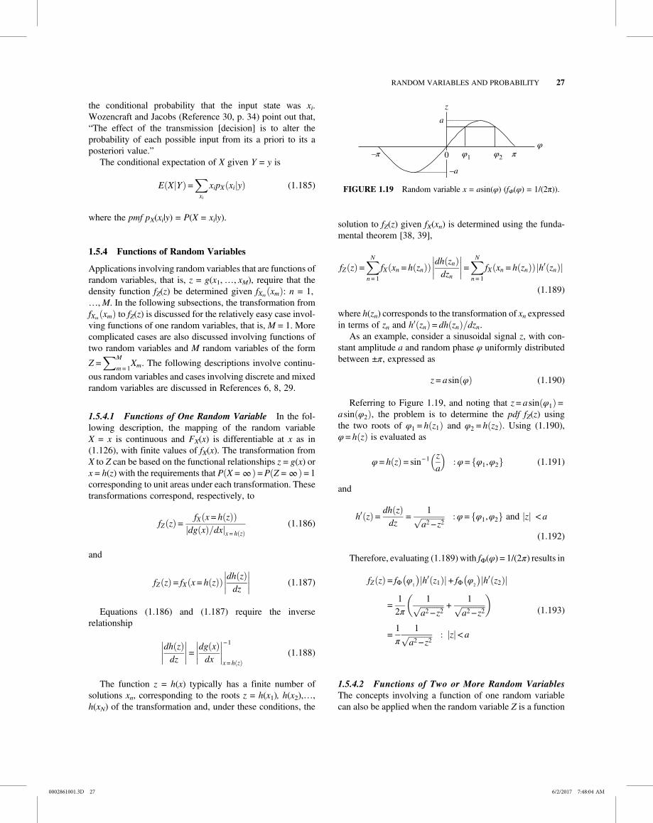
the conditional probability that the input state was xi.Wozencraft and Jacobs (Reference 30, p. 34) point out that,“The effect of the transmission [decision] is to alter theprobability of each possible input from its a priori to its aposteriori value.”

The conditional expectation of X given Y = y is

E X Y =xi

xipX xi y (1.185)

where the pmf pX(xi|y) = P(X = xi|y).

1.5.4 Functions of Random Variables

Applications involving random variables that are functions ofrandom variables, that is, z = g(x1,…, xM), require that thedensity function fZ(z) be determined given fXm xm : n = 1,…,M. In the following subsections, the transformation fromfXm xm to fZ(z) is discussed for the relatively easy case invol-ving functions of one random variables, that is, M = 1. Morecomplicated cases are also discussed involving functions oftwo random variables and M random variables of the form

Z =M

m = 1Xm. The following descriptions involve continu-

ous random variables and cases involving discrete and mixedrandom variables are discussed in References 6, 8, 29.

1.5.4.1 Functions of One Random Variable In the fol-lowing description, the mapping of the random variableX = x is continuous and FX(x) is differentiable at x as in(1.126), with finite values of fX(x). The transformation fromX to Z can be based on the functional relationships z = g(x) orx = h(z) with the requirements that P X = ∞ =P Z = ∞ = 1corresponding to unit areas under each transformation. Thesetransformations correspond, respectively, to

fZ z =fX x = h z

dg x dx x= h z

(1.186)

and

fZ z = fX x= h zdh z

dz(1.187)

Equations (1.186) and (1.187) require the inverserelationship

dh z

dz=

dg x

dx

−1

x = h z

(1.188)

The function z = h(x) typically has a finite number ofsolutions xn, corresponding to the roots z = h(x1), h(x2),…,h(xN) of the transformation and, under these conditions, the

solution to fZ(z) given fX(xn) is determined using the funda-mental theorem [38, 39],

fZ z =N

n = 1

fX xn = h zndh zndzn

=N

n= 1

fX xn = h zn h zn

(1.189)

where h(zn) corresponds to the transformation of xn expressedin terms of zn and h zn = dh zn dzn.

As an example, consider a sinusoidal signal z, with con-stant amplitude a and random phase φ uniformly distributedbetween ±π, expressed as

z = asin φ (1.190)

Referring to Figure 1.19, and noting that z= asin φ1 =asin φ2 , the problem is to determine the pdf fZ(z) usingthe two roots of φ1 = h z1 and φ2 = h z2 . Using (1.190),φ= h z is evaluated as

φ= h z = sin−1 z

aφ= φ1,φ2 (1.191)

and

h z =dh z

dz=

1

a2−z2φ= φ1,φ2 and z < a

(1.192)

Therefore, evaluating (1.189) with fΦ(φ) = 1/(2π) results in

fZ z = fΦ φ1

h z1 + fΦ φ2

h z2

=12π

1

a2−z2+

1

a2−z2

=1π

1

a2−z2z < a

(1.193)

1.5.4.2 Functions of Two or More Random VariablesThe concepts involving a function of one random variablecan also be applied when the random variable Z is a function

–a

a

1 2

z

φ φφ

π–π 0

FIGURE 1.19 Random variable x = asin(φ) (fΦ(φ) = 1/(2π)).

0002861001.3D 27 6/2/2017 7:48:04 AM


of several random variables; for example, the dependence ontwo random variables, such that, z = g(x,y) is discussed atlength by Papoulis (Reference 8, Chapters 6 and 7) wherethe subjects involving marginal distributions, joint densityfunctions, probability masses, conditional distributions anddensities, and independence are introduced. According to(1.126), the probability density function fZ(z) is determinedfrom the distribution function FZ(z) as

fZ z =∂FZ z

∂z(1.194)

and the joint pfd of X and Y is characterized for continuousdistributions as

fXY x,y =∂2FXY x,y

∂x∂y(1.195)

where the joint cdf is given by

FXY x,y =y

−∞

x

−∞fXY x ,y dx dy (1.196)

Based on the conditions for the equality of the probabil-ities, that is,

PZ Z ≤ z =PXY x,y g x,y ≤ z

the pdfs are equated as

FZ z =FXY g x,y ≤ z =g x,y ≤ z

fX,Y x,y dxdy (1.197)

Upon differentiating (1.197) with respect to z yields thedesired result expressed as

fZ z =∂FZ z

∂z=

∂

∂z g x,y ≤ zf x,y dxdy (1.198)

As an example application consider the random variableZ = X + Y; Papoulis states that, “This is the most importantexample of a function involving two random variables.”Upon letting y = z – x and using (1.198) the density functionof Z is evaluated as

fZ z =∂

∂z

∞

−∞

z−x

−∞f x,y dxdy =

∞

−∞fXY x,z−x dx

(1.199)

and, when X and Y are independent, (1.199) is simply theconvolution of fX(x) with fY(y). Several examples involvingthe use of (1.199) are given in Section 1.5.6.1.

Using the joint probability density function of two contin-uous random variables x and y, as expressed in (1.195), the

marginal pdfs fX(x) and fY(y) are obtained by integrating overy and x, respectively, resulting in

fX x =∞

−∞fXY x,y dy (1.200)

and

fY y =∞

−∞fXY x,y dx (1.201)

These results can also be generalized to apply to the jointdensity function of any number of continuous random vari-ables by integrating over each of the undesired variables.

1.5.5 Probability Density Functions

The following two subsections examine the probability den-sity function [40] of the magnitude and phase of a sinusoidalsignal with additive noise and the probability density func-tion of the product of two zero-mean equal-variance Gaussiandistributions. In these cases, the random variables of interestinvolve functions of two random variables. In Section 1.5.6,the characteristic function is defined and examined forseveral probability distribution functions demonstrating thecentral limit theorem with increasing summation of randomvariables. In Section 1.5.7, many of the probability distribu-tions used in the following chapters are summarized andcompared.

1.5.5.1 Distributions of Sinusoidal Signal Magnitudeand Phase in Narrowband Additive White Gaussian NoiseThis example involves the evaluation of the pdf of the mag-nitude and phase at the output of a narrowband filter when theinput is a sinusoidal signal with uniformly distributed phaseand zero-mean additive white Gaussian noise [41] (AWGN).In this case, the output of the narrowband filter is anarrowband random process. The evaluation involves threerandom variables: the input signal phase φ and the two inde-pendent-identically distributed (iid) zero-mean quadraturenoise random variables with variance σ2n. The signal plusnoise out of the filter is expressed as

s t =Acos ωct +φ + n t cos ωct +ϕ t

=Acos φ cos ωct −Asin φ sin ωct

+ n t cos ϕ t cos ωct −n t sin ϕ t sin ωct

= Acos φ + nc t cos ωct − Asin φ + ns t sin ωct

(1.202)

where the third equality in (1.202) emphasizes the in-phaseand quadrature functions of the signal and noise terms and,when sampled at t = iTs, represent the random variables

0002861001.3D 28 6/2/2017 7:48:05 AM


xc, nc, xs, and ns. The functional relationships arexc =Acos φ + nc and xs =Asin φ + ns with nc and ns repre-senting zero-mean quadrature Gaussian random variables.The signal phase, φ, is uniformly distributed between 0and 2π. Under these conditions, the quadrature signal andnoise components xc and xs are independent random vari-ables* and the pdfs of xc and xs are expressed as

fXc xc =1

2πσne− xc−Acos φ 2 2σ2n (1.203)

and

fXs xs =1

2πσne− xs −Asin φ 2 2σ2n (1.204)

The pdf of the phase is

fΦ φ =12π

0 ≤φ ≤ 2π (1.205)

Using (1.203), (1.204), and (1.205) the joint pdf isexpressed as

fXc , Xs,Φ xc,xs,φ = fXc xc fXs xs fΦ φ

=1

4π2σ2e−

xc −Acos φ 2 + xs −Asin φ 2

2σ2

(1.206)

The evaluation of the joint pdf of the magnitude and phaseof the sampled sine-wave plus noise involves the transfor-mation of variables from (xc,xs) to (r,θ) as depicted inFigure 1.20. The magnitude is described as

r = s iTs = x2c + x2s (1.207)

and the in-phase and quadrature components, xc and xs, aredescribed in terms of the angle θ as

xc = rcos θ and xs = r sin θ (1.208)

Expressing the phase angle in (1.208) as a function of xcand xs leads to the expressions

θ = cos−1xcx2c + x2s

(1.209)

and

θ = sin−1 xsx2c + x2s

(1.210)

The Jacobian of the transformation is defined as [6, 8,28, 29]

J xc,xs ≜∂g11 xc,xs

∂xc

∂g12 xc,xs∂xs

∂g21 xc,xs∂xc

∂g22 xc,xs∂xs det

(1.211)

and, using the Jacobian, the transformation from (xc,xs) to(r,θ) is expressed as

fR,Θ,Φ r,θ,φ =fXc , Xs,Φ h1 r,θ ,h2 r,θ ,φ

J xc,xs(1.212)

To evaluate the Jacobian for this transformation, the func-tions gij(xc,xs) are defined in terms of (1.207), (1.209), and(1.210) as follows:

g11 xc,xs = g12 xc,xs = x2c + x2s (1.213)

g21 xc,xs = cos−1xcx2c + x2s

(1.214)

and

g22 xc,xs = sin−1 xsx2c + x2s

(1.215)

Upon evaluating the partial derivatives in (1.211), theJacobian is found to be†

J xc,xs =1

x2c + x2s=1r

(1.216)

xs

0

rθ

xc

FIGURE 1.20 Relationship between transformation variables.

*Orthogonal Gaussian random variables are also independent.

†The phase angle can also be expressed as θ = tan−1(xs/xc) with the Jacobianevaluated as earlier using, g21(xs, xc) = g22(xs, xc) = tan−1(xs/xc) (seeProblem 16).

0002861001.3D 29 6/2/2017 7:48:06 AM


and, using (1.208), the functions h1(r,θ) and h2(r,θ) areexpressed as

h1 r,θ = xc r cos θ = rcos θ (1.217)

and

h2 r,θ = xs r sin θ = r sin θ (1.218)

Substituting (1.216), (1.217), and (1.218) into (1.212) andapplying the independence of xc, xs, and φ, as in (1.206), thepdf of the transformed variables r and θ is expressed as

fR,Θ,Φ r,θ,φ = fR r fΘ θ fΦ φ

=r

4π2σ2e−

rcos θ −Acos φ 2 + rsin θ −Asin φ 2

2σ2

=r

4π2σ2e−

r2 + A2 −2Arcos θ−φ2σ2

(1.219)

where r ≥ 0, otherwise the pfd is zero, and θ and φ areuniformly distributed over the range 0 ≤ θ, φ ≤ 2π. The pdffor the magnitude r is determined by computing the marginaldistribution MR(r) by integrating over the ranges of θ and φ.Defining ψ = θ − φ, the marginal is evaluated as

fR r =r

σ2e−

r2 + A2

2σ212π

2π

0

12π

2π−φ

φ

eArcos ψ σ2dψ dφ

(1.220)

Davenport and Root [42] point out that the integrand of thebracketed integral is periodic in the uniformly distributedphase ψ and can be integrated over the interval 0 to 2π. Withthis integration range, the bracketed integral is identified asthe zero-order modified Bessel function expressed as [43]

IoAr

σ2=

12π

2π

0

eArcos ψ σ2dψ (1.221)

Therefore, upon using (1.221) and performing the integra-tion over φ, the marginal distribution function MR(r) simpli-fies, at least in notation, to

fR r =r

σ2e−

r2 + A2

2σ2 IoAr

σ2(1.222)

Equation (1.222) is the Rice distribution or, as referred tothroughout this book, the Ricean distribution that, as devel-oped in the forgoing analysis, characterizes the baseband

magnitude distribution of a CW signal with narrowband addi-tive white Gaussian noise. The Ricean distribution also char-acterizes the magnitude distribution of a received signal froma channel with multipath interference; this channel is referredto as a Ricean fading channel. The Ricean distributionbecomes the Rayleigh distribution as A 0 and the Gaussiandistribution as A ∞; the proof of these two limits is thesubject of Problems 19 and 20. The Rayleigh distributioncharacterizes the amplitude distribution of narrowband noiseor, in the case of multipath interference, the composite signalmagnitude of many random scatter returns without a domi-nant specular return or signal component. The multipathinterference is the subject of Chapter 18. Defining thesignal-to-noise ratio as γ = A2/(2σ2), (1.222) is expressed as

fR r =r

σ2e− r2 2σ2 + γ Io

r 2γσ

(1.223)

The pdf of the phase function is evaluated by computingthe marginal distribution MΘΦ(θ,φ) by integrating over therange of the magnitude r. By forming or completing thesquare of the exponent in the last equality in (1.219) the inte-gration is performed as

fΘΦ θ,φ =1

4π2σ2e−Asin

2 θ−φ 2σ2∞

0re− r−Acos θ−φ 2 2σ2dr

(1.224)

Davenport and Root [44] provide an approximate solutionto (1.224), under the condition Acos(θ – φ) >> σ. The approx-imation is expressed as

fΘΦ θ,φAcos θ−φ

2π 3 2σe−γsin

2 θ−φ 0 ≤ θ,φ ≤ 2π (1.225)

where γ is the signal-to-noise ratio defined earlier. An alter-nate solution, without the earlier restriction, is expressed byHancock [45], with ψ = θ − φ, as

fΨ ψ =e−γ

2π1 + 4πγcos ψ eγcos

2 ψ P 2γcos ψ

−π ≤ψ ≤ π

(1.226)

where P(z) is the probability integral defined in Section 3.5.Hancock’s phase function is used in Section 4.2.1 to charac-terize the performance of phase-modulated waveforms.

As γ 0 in (1.226) the function fΨ(ψ) 1/2π resulting inthe uniform phase pdf. However, for γ greater than about 3,the probability integral is approximated as [26]

P z 1−e− z

2 2

2πzz > 3 (1.227)

0002861001.3D 30 6/2/2017 7:48:06 AM


Using (1.227), the phase pdf is approximated as

fΨ ψγ πcos ψ e−γsin

2 ψ 1 > cos ψ > 2 5 γ

0 −2 5 γ > cos ψ > −1

(1.228)

With |ψ | 0 such that sin2(ψ) ψ2 and definingγ = 1 2σ2ψ (1.228) is approximated as

fΨ ψ1

2πσψe−ψ

2 2σ2ψ ψ 0 and γ = 1 2σ2ψ (1.229)

Equation (1.229) describes a zero-mean Gaussian phasepdf with the phase variance σ2ψ = 1 2γ. Hancock’s phasefunction, expressed in (1.226), is plotted in Figure 4.3 for var-ious signal-to-noise ratios.

1.5.5.2 Distribution of the Product of Two IndependentGaussian Random Variables In this section the pdf ofthe product z = xy of two zero-mean equal-variance iid Gaus-sian random variables X and Y is determined. The solutioninvolves defining an auxiliary random variable w = h(x) = xwith z = g(x,y) = xy and evaluating fZ,W(w,z) characterized as

fW ,Z w,z =fX,Y w,z w

JX,Y x,y(1.230)

where JX,Y(x,y) is the Jacobian of the transformation evalu-ated as

JX,Y x,y =

∂g x,y∂x

∂g x,y∂y

∂h x,y∂x

∂h x,y∂y det

= −x (1.231)

Using (1.231) and the joint Gaussian pfd of X and Y,expressed by (1.230), with x = w and y = z/w, the marginalpdf of z is evaluated as

fZ z =∞

−∞

1w

fX,Y w,z w dw (1.232)

However, since X and Y are independent

fX,Y x,y = fX x fY y =1

2πσ2e−

x2 + y2

2σ2 (1.233)

and, upon substituting x = w and y = z/w into (1.233), (1.232)is expressed as

fZ z =1

2πσ2

∞

−∞

1w

e−w2 + z w 2

2σ2 dw

=1πσ2

∞

0

1we−

w2 + z w 2

2σ2 dw

(1.234)

where the second equality recognizes that the first equality issymmetrical in w. Letting λ = w2/2σ2 (1.234) is expressed as

fZ z =1

2πσ2

∞

0

1λe− λ + z2

4σ4 λ dλ (1.235)

The solution to the integral in (1.235) appears in thetable of integrals by Gradshteyn and Ryzhik (Reference46, p. 340, pair No. 12) as

∞

0λv−1e

− λ+ u2

4λ dλ= 2u

2

vK−v u (1.236)

whereKv(u) is the modified Bessel function of the second kindof order v. With v = 0 and u = z/σ2, (1.235) is evaluated as

fZ z =1πσ2

Koz

σ2(1.237)

The magnitude of z in (1.237) is used because of the evensymmetry of fZ(z) with respect to z. The symmetry of fZ(z)results in a zero-mean value so the variance is evaluated as

Var z =E z2 zero-mean

=2πσ2

∞

0z2Ko

z

σ2dz

(1.238)

The solution to the integral in (1.238) is found in Gradsh-teyn and Ryzhik (Reference 46, p. 684, Integral No. 16) andthe variance fZ(z) is evaluated as

Var z =4πΓ2 3

2σ4 = σ4 (1.239)

where the second equality in (1.239) results from the value ofthe Gamma function Γ 3 2 = π 2. In Example 4 ofSection 1.5.6.1, the pdf of the summation of N iid randomvariables with pdfs expressed by (1.237) is examined.

1.5.6 The Characteristic Function

The characteristic function of the random variable X isdefined as the average value of ejvx and is expressed as

CX v ≜E ejvx =∞

−∞fX x ejvxdx (1.240)

0002861001.3D 31 6/2/2017 7:48:07 AM


With v = −ω and x = t (1.240) is similar to the Fouriertransform of a time-domain function. The characteristic func-tion is also referred to as the moment-generating function, inthat, the nth moment of the random variable X, defined as theexpected value E[xn], is evaluated (see Problem 26) as

E xn = − j ndnCX v

dvn v = 0

(1.241)

The Fourier transform relationship between time domainconvolution and frequency domain multiplication alsoapplies to the convolution of random variables and the mul-tiplication of the corresponding characteristic functions.Therefore, based on the discussion in Section 1.5.6.1, thesummation of N identically distributed (id) random variablescorresponds to the product of their individual characteristicfunctions, that is,

CZ v =N

i= 1

CXi v Z = Xi, i = 1,…,N; Xi id

(1.242)

This is a very useful result, in that, the distribution of thesummation of N independent random variables is obtained asthe inverse transform [47] of (1.242) expressed as

fZ z =∞

−∞CZ v e− jvzdz (1.243)

Campbell and Foster [47] provide an extensive listing ofFourier transform pairs defined as

G g =∞

−∞F f ej2πfgdf and F f =

∞

−∞G g e− j2πfgdg

(1.244)

and, by defining v = −2πf, the Fourier transform pairs applyto the transform pairs between fX(x) and CX(v) as expressedin (1.240).

1.5.6.1 Summation of Independently Distributed RandomVariables If two random variables X and Y are independentthen the probability density fZ(z) of their sum Z = X + Y isdetermined from the convolution of fX(x) with fY(y) so that*

fZ z =∞

−∞fX z−y fY y dy=

∞

−∞fX x fY z−x dx (1.245)

For multiple summations of a random variable, the convo-lution is repeated for each random variable in the summation.

Example 1 Consider the summation of N zero-mean uni-formly distributed random variables Xi expressed as

Z =N

i= 1

Xi 1 246

with

fX x =12a

−a ≤ x ≤ a (1.247)

For N = 2 the convolution involves two ranges of thevariable z as shown in Figure 1.21 and the integrations areevaluated as

fZ z =14a2

z+ a

−adx −2a ≤ z ≤ 0 (1.248)

and

fZ z =14a2

a

z−adx 0 ≤ z ≤ 2a (1.249)

Upon evaluation of (1.248) and (1.249) and recognizingthe symmetry about z the density function is expressed as

fZ z =12a

−z

2a+ 1 z ≤ 2a (1.250)

Repeating the application of the convolution for N = 3and 4 (see Problem 24) results in the probability density func-tions shown in Figure 1.22 with the corresponding cdf resultsshown in Figure 1.23. As N ∞ the probability density andcharacteristic functions will approach those of the Gaussiandistributed random variable (see Problem 23).

x

x

x

z + a

0 a–a

f(x)

1/2a

z

Range 1:–2a ≤ z ≤0

z

Range 2:0 ≤ z ≤ 2a

z – a

1/2a

1/2a

FIGURE 1.21 Convolution of two zero-mean uniformdistributions.

*For proof see Reference 8, p. 189.

0002861001.3D 32 6/2/2017 7:48:07 AM


The moments of the random variable X are evaluatedusing the characteristic function

CX v =sin av

av(1.251)

In regions where the characteristic function converges, themoments E[xn] completely define the characteristic functionand the pdf of the random variable X, so, upon expanding(1.251) as the power series

CX v = 1−av 2

3+

av 4

5− (1.252)

the moments are easily evaluated using (1.241). Themoments for the random variable Z, formed as in (1.246),are determined using (1.242) and, with Xi : i = 1,…,Niid random variables, the characteristic function for Z isapproximated as

CZ v =CNX v 1−

N av 2

3(1.253)

The first and second moments for N = 1, …, 4 are listedin Table 1.6. These results are also obtained by evaluatingfZ(z) using (1.250) and then evaluating the moments (seeProblem 25) as

E zn =Na

−NaznfZ z dz (1.254)

However, it is much easier to use the characteristicfunction.

Example 2 As another example, consider the summation ofN random variables Xi characterized as the sinusoidalfunction

Xi =Ai sin Φi 1 255

with constant amplitudes Ai and zero-mean uniformly distrib-uted phase, expressed as

fΦ φ =12ϕ

φ ≤ϕ (1.256)

The resulting pdf of the random variable Xi for ϕ = π, isevaluated in (1.193) as

fX xi =1

π A2i − x2i

(1.257)

and is plotted in Figure 1.24.

z–4 –3 –2 –1 0 1 2 3 4

f Z(z

)

0.000

0.125

0.250

0.375

0.500

N = 23

4

FIGURE 1.22 pdf for sum of N = 2, 3 and 4 independent zero-mean uniform distributions (a = 1).

z–4 –3 –2 –1 0 1 2 3 4

FZ(

z)

0.00

0.25

0.50

0.75

1.00N = 2

43

FIGURE 1.23 cdf for sum of N = 2, 3 and 4 independent zero-mean uniform distributions (a = 1).

TABLE 1.6 Moments of fZ(zN) forZ= Xi i = 1,…,4, Xi iid Zero-MeanUniform Distributions

N E[z] E[z2]

1 0 a2/32 0 2a2/33 0 a2

4 0 4a2/3

0002861001.3D 33 6/2/2017 7:48:08 AM


The pdf of the random variable Z, expressed as in (1.246),*

is evaluated by successive convolutions as in (1.245) and theresults for N = 2, 3, and 4 are plotted in Figure 1.25 with thecorresponding cdf functions shown in Figure 1.26. Theresults in Figures 1.25 and 1.26 for N > 1 are obtained bynumerical evaluations of the convolutions using incrementalvalues of Δz = 2.5 × 10−5; this is a reasonable compromisebetween simulation time and fidelity in dealing with the infi-nite value at |x| = 1.0.

In this case, the mean and variance of the random variableX are evaluated using the characteristic function of (1.257)

found in (Reference 47, p. 123, Transform Pair 914.5); theresult is

CX v = Io − jAv (1.258)

where Io(−) is the modified Bessel function of orderzero. Expanding (1.258) for Av < 1 as a power series,(Reference 46, p. 375, Ascending Series 9.6.10), results in†

CX v = 1−Av 2

4 1 2 +Av 4

42 2 2 −Av 6

43 3 2 (1.259)

and the moments are easily evaluated using (1.241). The firstand second moments are listed as the theoretical values inTable 1.7. The moments for the random variable Z, formedas in (1.246) with Xi iid random variables for all i as expressedby the pdf in (1.255), are determined using the characteristicfunction expressed as

z–4 –3 –2 –1 0 1 2 3 4

f Z(z

)

0.00

0.25

0.50

0.75

1.00

3

4

N = 2

FIGURE 1.25 pdf of N = 2, 3, and 4 successive convolutionsof fX(x).

z–4 –3 –2 –1 0 1 2 3 4

FZ(z

)

0.00

0.25

0.50

0.75

1.00N = 1 2 3

4

FIGURE 1.26 cdf of N = 2, 3, and 4 successive convolutionsof fX(x).

x–1.0 –0.5 0.0 0.5 1.0

f X(x

)

0.0

0.5

1.0

1.5

2.0

2.5

3.0

3.5

4.0

FIGURE 1.24 pdf of x = Asin(φ) with zero-mean uniformlydistributed phase, A = 1 and ϕ = π.

TABLE 1.7 Moments of fZ(zN) for Z= Xi i= 1,…,N, Xi iid

Random Variables Expressed by (1.255)

N

Theoretical Numericala (A = 1)

E[z] E[z2] E[z] E[z2]

1 0 A2/2 0 0.49992 0 A2 0 1.00443 0 3A2/2 0 1.50554 0 2A2 0 2.0146

aNumerical values are sampled with Δz = 2.5 × 10−5.

*By forming the average summation Z = 1 NN

i= 1xi, the range of the pdf

is limited to ±a with an associated decrease in the standard deviation.

†By comparing the ascending series expansion of Io(z) with that of the Besselfunction Jo(z) it is found that Io(−jz) = Jo(z).

0002861001.3D 34 6/2/2017 7:48:08 AM


CZ v =CNX v 1−

N Av 2

4 1 2 (1.260)

The corresponding first two moments of the random var-iable Z for N = 2, 3, and 4 are also listed in Table 1.7. Thenumerical results listed in Table 1.7 are based on computerevaluations of the various convolutions resulting in the pdfsshown in Figures 1.24 and 1.25.

A major observation in these two examples is that theprobability distribution of the random variable Z approachesa Gaussian distribution as N increases (see Problem 27). Thisis evidence of the central limit theorem which states that (seeDavenport and Root, Reference 6, p. 81) the sample mean ofthe sum of N arbitrarily distributed statistically independentsamples becomes normally distributed as N increases. This isreferred to the equal-components case of the central limit the-orem. However, as pointed out by Papoulis (Reference 8,p. 266), a consequence of the central limit theorem is thatthe distribution fZ(z) of the sum of N statistically independentdistributions having arbitrary pdf’s tends to a normal distri-bution as N increases. This is a stronger statement and sug-gests that the probability P(z) = fZ(Z < z) can be considered aGaussian distribution for all z as is frequency assumed to bethe case in practice. Davenport and Root also point out that,even though N is seemingly large, the tails of the resultingdistribution may result in a poor approximation to theGaussian distribution.

Upon computing the mean and variance using the powerseries expansion of CZ(v) expressed by (1.252) with av << 1,the approximate expression for the corresponding Gaussiandistribution is easily obtained. After summing N uniformlydistributed amplitudes the expression for the pdf is

fZ z =1

2πNa2 3e− z

2 2Na2 3 z = xi, i= 1,…,N,

p xi =12a

, xi ≤ a

(1.261)

Similarly, for the summation of N sinusoids with Av << 1,the pdf in Example 2 is expressed as

fZ z =1

2πNA2 2e− z

2 2NA2 2

z = xi, i= 1,…,N, xi =Asin φi

p φi =12π

, φi ≤ π

(1.262)

It is interesting to note that the second moments are Nλ2

for all values of N including those for which the pdf doesnot have the slightest resemblance to the Gaussian pdf.

In these cases, the important difference is that the corres-ponding probabilities P(x) = FX(X < x) are entirely differentfrom those of the Gaussian distribution with the possibleexception of the median value. Finally, it is noted that thelimiting behavior for λv << 1 and N ∞ applies to the sum-mation of independently distributed distributions that may,or may not, be identically distributed distributions.

Example 3 This example involves the summation ofrandom chips {±1} in a direct-sequence spread-spectrum(DSSS) waveform. In this case, the chips occur with equalprobabilities according to the pdf expressed as

fX x =12δ x−1 +

12δ x + 1 1 263

Using (1.240), the characteristic function is evaluated as

CX v =∞

−∞fX x ejvxdx

=12

∞

−∞ejvxδ x−1 dx+

∞

−∞ejvxδ x+ 1 dx

= cos v

(1.264)

The DSSS waveform uses N chips per bit and the demod-ulator correlation sums the N chips to form the correlation

output y =N−1

n= 0xn with the corresponding characteristic

function given by

CY v =CNX x = cosN v

= 1−v2

2+v4

4−v6

6+

N

= 1−Nv2

2+

(1.265)

To evaluate the first and second moments of y only thefirst two terms in the expansion of cosN(v) are requiredand, upon using (1.241), these moments are evaluated as

E x = j2Nv2 v = 0

= 0 first moment mean value, x

(1.266)

and

E x2 = −1−2N2 v = 0

=N second moment (1.267)

0002861001.3D 35 6/2/2017 7:48:10 AM


The variance of y is defined as the second central

moment E x−x 2 =E x2 −x2 and with zero-mean the var-

iance is σ2y =E x2 =N.

Example 4 The pdf fZ(z) of the product of two, zero-mean,equal-variance, iid Gaussian random variables, z = xy, isexpressed in (1.237) as a function of the zero-order modifiedBessel function Ko(|z|/σ

2) where the magnitude of z providesfor the range: −∞ ≤ z ≤∞. In this example, the pdf fZ z

is evaluated where Z =iZi : i = 1,…,N. The evaluation

is based on the N-th power of the characteristic functionCZ(v) and, from the work of Campbell and Foster(Reference 47, p. 60, pair No. 558), the characteristic func-tion is evaluated as*

CZ v =1 σ2

1 σ4−p2(1.268)

The characteristic function of Z is the N-th power of(1.268) expressed as

CNZ v =

1 σ2N

1 σ4−p2 N 2(1.269)

and, using the transform pair of Campbell and Foster(Reference 47, p. 61, pair No. 569.0), the pdf of Z is evaluatedas

fZ z =1 σ2N

πΓ N 2 2 σ2 N−1 2z N−1 2K N−1 2

z

σ2

(1.270)

As in the case for fZ(z), the pdf fZ z applies for −∞ ≤ z ≤∞and is symmetrical with respect to z resulting in a zero-meanvalue with the variance expressed as

Var z =E z2 with zero-mean

=2 σ2N

πΓ N 2 2 σ2 N−1 2

∞

0z2z N−1 2K N−1 2

z

σ2dz

(1.271)

The solution to the integral in (1.271) is found inGradshteyn and Ryzhik (Reference 46, p. 684, Integral No.16) and the variance fZ(z) is evaluated using

∞

0

zuKv az dz=2u−1

au + 1Γ

1 + u + v2

Γ1 + u−v

2(1.272)

Substituting the solution to the integral in (1.272) into(1.271), with u = (N + 3)/2, v = (N − 1)/2, and a = 1/σ2,the solution to variance simplifies to

Var z =Nσ4 (1.273)

In the earlier evaluation, the integer argument Gammafunction is related to the factorial as Γ N = N−1 ! andΓ 3 2 = π 2. This result could also be evaluated usingthe movement generating function of (1.241), however, usingthe integral solution as in (1.272) it is sometimes easierto evaluate the moments. With a sufficiently large valueof N the pdf fZ z is approximated as the Gaussian pfdexpressed as

fZ zN ∞

1

2πNσ4e−z

2 2Nσ4 zero-mean Gaussian pdf

(1.274)

The probability density functions discussed earlier andothers encountered in the following chapters are summarizedin Table 1.8 with the corresponding mean values, variances,and characteristic functions.

1.5.7 Relationships between Distributions

In the following two subsections, the relationship betweenvarious probability density functions is examined by straight-forward parameter transformations, allowing parameters toapproach limits, or simply altering various parameter values.The most notable relationship is based on the central limittheorem in which a distribution approaches the Gaussiandistribution by increasingly summing the operative randomvariable.

1.5.7.1 Relationship between Chi-Square, Gaussian,Rayleigh, and Ricean Distributions A random variablehas a chi-square (χ2) distribution with N degrees of freedomif it has the same distribution as the sum of the squares ofN-independent, normally distributed random variables, eachwith zero-mean and unit variance.†

Consider the zero-mean Gaussian or normal distributedrandom variable x with variance σ2x and pdf expressed as

pX x =1

2πσxe− x

2 2σ2x (1.275)

The pdf of a new random variable y = x2, obtained by sim-ply squaring x, is determined by considering the positive andnegative regions of x = ± y as shown in Figure 1.27.

*The tables of Campbell and Foster are Fourier transform pairs that corre-spond to characteristic function pairs with p = −jv.

†A normally distributed random variable x with mean value mx and varianceσ2x can be transformed into a zero-mean, unit-variance normally distributedrandom variable y by substituting y = (x −mx)/σx.

0002861001.3D 36 6/2/2017 7:48:10 AM


The pdf of y is determined using the incremental intervalsdy = 2xdx at x= ± y such

pY y = pX x = ydx

dy+ pX x = − y

dx

dyU y

=1

2πσxe−y 2σ2x + e−y 2σ2x

12 y

U y

=e−y 2 σ2x

2πyσxU y

(1.276)

TABLE 1.8 Probability Distributions and Characteristic Functions

Name fX(x) E[x] Var[x] CX(v) Conditions

Uniform 1b−a

a+ b2

b−a 2

12

ejvb−ejva

jv b−a

a ≥ x ≤ b

Bernoulli p i= 1

1−p i= 2

p p(1 − p) (1 − p) + pv Discrete binary variablex = ki : i = 1, 2

Binomial n

kpk 1−p n−k

np np(1 – p) 1−p + pv n Discrete variablex= k = 1,2,…,n

Poisson αke−α k! α α eα v−1 Discrete variablex= k = 0,1,…; α> 0

Exponential αe−αx 1/α 1/α2 α α− jv x ≥ 0; α > 0

Gaussian (normal)e−

x−m 2

2σ2

2πσ

m σ2e− jmv−

σ2 v2

2−∞ ≤ x ≤ ∞

Chi-square (N = 2)Exponential (α = 1/2)

e−x 2

2

2 4 1− j2v −1 x ≥ 0

Chi-squared (N-degrees) xN 2−1e−x 2

2N 2 N 2−1

N 2N 1− j2v −N 2 N-degrees of freedom x ≥ 0

Rayleigh xe− x2 2σ2

σ2π 2σ as γ ∞ 4−π σ2

2as γ ∞

1− jv β α x > 0

Riceanxe−

x2 −A2

2σ2

σ2Io

xA

σ2

a a a x > 0

A2 2σ2 ∞

A2 2σ2 = 0

Gamma β βx α−1

Γ αe−βx

α/β α/β2 1

1− j vβα

x > 0β > 0; λ > 0

Lognormale−

ln y −m 2

2σ2

2πyσ

em + σ2 2 em+ 2σ2

−em+ σ2

b y is lognormaly = ex ≥ 0x = N(m,σ)

Nakagami-m 2mmx2m−1e−mx2 Ω

Γ m Ωm

c c c x ≥ 0

m =E x2

2

E x2−E x2 2

≥ 1 2

Notes: γ = A2/(2σ2) is the signal-to-noise ratio. γ 0 fX(x) = Rayleigh with E[x] = π 2σ, Var[x] = 4−π σ2 2.aγ ∞ fX(x) = Gaussian with E[x] = A, Var[x] = σ2.bApproximated using a series expansion of ejvy.cRefer to special cases in Section 1.5.7.2.

x–x

y

0

y

x

FIGURE 1.27 Transformation of the random x to y = x2.

0002861001.3D 37 6/2/2017 7:48:11 AM


The characteristic function of (1.276) is evaluated as

C1Y v =E pY y ejvy =

1

1− j2 σ2xv1 2

(1.277)

Consider now the random variable z resulting from thesummation of N independent random variables yi such that

z=N

i= 1

yi =N

i= 1

x2i (1.278)

The characteristic function of z is simply the N-th powerof CY(v) so that

CNZ v = C1

Y vN

=1

1− j2 σ2xvN 2

(1.279)

Equation (1.279) transforms to the pdf of z, resulting in

pZ z =zN 2−1e−z 2 σ2x

2 σ2xN 2 N

2−1

U y (1.280)

In conforming to the earlier definition, the chi-squaredistribution is expressed by letting σ2x = 1 in (1.280) or, moreformally, using the transformation χ = z σ2x ; therefore, thepdf of the chi-square random variable χ with N degrees offreedom is

pX χ =χN 2−1e−χ 2

2N 2 N

2−1

U y Chi-square distribution

(1.281)

and the corresponding characteristic, or moment generating,function is

CNX v =

1

1− j2v N 2Chi-square characteristic function

(1.282)

Equation (1.281) is occasionally referred to as the centralχ2 distribution because it is based on noise only, that is,the underlying zero-mean Gaussian random variables xi

with distribution given by (1.275) do not contain a signalcomponent.*

Special Case for N = 2 Under this special case z = x21 + x22

(1.280) reduces to the exponential distribution

pZ z =e−z 2 σ2x

2 σ2xU y exponential distribution (1.283)

So the resulting chi-square χ2 distribution is obtained from(1.281) with N = 2. This is an important case because x1 andx2 can be thought of as orthogonal components in the com-plex description of a baseband data sample. Urkowitz [48]shows that the energy of a wide-sense stationary narrowbandwhite noise Gaussian random process with bandwidth –W toW Hz and measured over a finite interval of T seconds isapproximated by N = 2WT terms or degrees of freedom.The frequency W is the noise bandwidth of the narrowbandbaseband filter and the approximation error in the energymeasurement decreases with increasing 2WT. The factor oftwo can be thought of as the computation of complex orthog-onal baseband functions z= x2c + jx

2s so N = 2 degrees of free-

dom correspond to WT = 1. For example, the rect(t/T)function observed over the interval T seconds has a noisebandwidth of W = 1/T Hz corresponding to WT = 1 resultingin 2 degrees of freedom.

Upon letting w= z = x2c + x2s , the random variable w is

described in terms of the Rayleigh distribution

pW w =w

σ2xe−w

2 2σ2x U y Rayleigh distribution (1.284)

So the Rayleigh distribution is derived from the magni-tude of the quadrature zero-mean Gaussian distributed ran-dom variables, x = N(0,σ).†

1.5.7.2 Relationship between Nakagami-m, Gaussian,Rayleigh, and Ricean Distributions The Nakagami-m dis-tribution [49] was initially derived from experimental data tocharacterize HF fading; however, subsequent experimentalobservations demonstrate its application to rapid fading atcarrier frequencies from 200 MHz to 4 GHz. It is consideredto be a generalized distribution from which other distri-butions can be derived, for example, m = 1 results in theRayleigh power distribution, m = ½ results in the one-sided

*When the underlying Gaussian distributed random variable is composed ofsignal plus noise, the signal amplitude represents the mean value of the dis-tribution. An analysis, similar to that of (1.276) through (1.280), containing amean value, results in a noncentral χ2 distribution with 1 through N degreesof freedom. The noncentral χ2 distribution is developed and discussed inAppendix C.†The notation N(m,σ) is used to denote the distribution of a Gaussian, or nor-mal, random variable with mean value m and standard deviation σ.

0002861001.3D 38 6/2/2017 7:48:12 AM


zero-mean Gaussian distribution, and as m ∞ them-distribution approaches the Gaussian distribution with aunit mean value. In the region 1 ≤ m ≤ ∞, the Nakagami-mdistribution behaves much like the Ricean distribution;however, the normalized distributions are subtly differentwhen plotted for various signal-to-noise ratios less thanabout 10 dB. The Ricean distribution, referred to as then-distribution by Nakagami, is derived from concepts invol-ving narrowband filtering of a continuous wave (CW) signalwith additive Gaussian noise, whereas the Nakagami-mdistribution is derived from experimental data involvingmultipath communication links.

1.5.8 Order Statistics

Communication systems analysis and performance evalua-tions often involve a large number of random samples takenfrom an underlying continuous or discrete probability distri-bution function. The various parameters, used to characterizethe system performance, result in limiting distributionswith associated means, variances, and confidence levels asdictated, for example, by an underlying distribution. Order sta-tistics [31, 50, 51], on the other hand, involves a distribution-free or nonparametric analysis that requires only thatthe probability distribution functions be continuous and notnecessary related to the underlying distribution from whichthe samples are taken. However, the randomly drawn samplesare considered to be statistically independent.

Consider that the n random samples {X1, X2, …, Xn} aretaken from the continuous pdf fX(x) over the range a ≤ x ≤ b.Now consider reordering the random variables Xi : i = 1,…, n to form the random variables {Y1, Y2,…, Y n} arrangedin ascending order of magnitude, such that, a ≤ Y1 < Y2 << Yn ≤ b where fYi yi = 1 b−a is uniformly distributedover the interval b − a. The joint pdf of the ordered samples[52] is expressed as

gY1,Y2,…,Yn y1,y2,…,yn = nn

i= 1

fYi yi (1.285)

for a ≤ y1 < y2 < < yn ≤ b and n! is the number of mutuallydisjoint sets of x1, x2,…, xn. For example, for n = 4 the setx1, x2, x3, x4 results in n! = 24 mutually disjoint sets deter-mined as shown in Table 1.9. The first six mutually disjointsets are determined by cyclically left shifting the indicatedsubsets of original set x1, x2, x3, x4; a cyclic left shift of asubset is obtained by shifting each element of the subset tothe left and replacing the leftmost element in the former posi-tion of the rightmost element. Following the first six setsshown in the figure, the original set is cyclically shifted threemore times each leading to six mutually disjoint sets by shift-ing subsets resulting in a total of 24 mutually disjoint sets.

The ordered sample Yi is referred to as the i-th order sta-tistic of the sample set. The marginal pfd of the n-th orderstatistic Yn, that is, the maximum of {X1, X2,…, Xn}, is eval-uated using (1.285) by performing the integrations in theascending order i = 1, 2, …, n − 1 as follows*:

gYn yn = nyn

a

y4

a

y3

a

y2

af y1 dy1 f y2 f yn dy2 dyn−1

= nyn

a

y4

a

y3

aF y2 f y2 dy2 f y3 f yn dy3 dyn−1

= nyn

a

12

y4

aF2 y3 f y3 dy3 f y4 f yn dy4 dyn−1

= n fYn yn1

n−2

yn

aFn−2 yn−1 f yn−1 dyn−1

(1.286)

The solution (see Problem 15) to (1.286) is

gYn yn = n F ynn−1fYn yn a < yn ≤ b (1.287)

where Fn−1(yn) is the cdf evaluated as

Fn−1 yn = n−1yn

aFn−2 yn−1 fY yn−1 dyn−1 =

yn−an−1

b−a n−1

(1.288)

Using the marginal pdf of Yn given by (1.287), the prob-ability of selecting the maximum of value Yn is determined as

P y = ny

aFn−1 yn fY yn dyn

y = b

= 1 (1.289)

TABLE 1.9 Example of Mutually Disjoint Sets (n = 4,24 Mutually Disjoint Sets)

No. Mutually Disjoint Sets Shiftinga

1 x1, x2, x3, x4 Original set2 x1, x2, x4, x3 Shift subset x3, x43 x1, x3, x4, x2 Shift subset x2, x3, x44 x1, x3, x2, x4 Shift subset x4, x25 x1, x4, x2, x3 Shift subset x3, x4, x26 x1, x4, x3, x2 Shift subset x2, x37 x2, x3, x4, x1 Shift original set8 x2, x3, x1, x4 Shift subset x4, x19 x2, x4, x1, x3 Shift subset x3, x4, x1

aShift denotes a cyclic left shift of a previous set or subset.

*For notational simplicity f(y) is used to denote fY(y).

0002861001.3D 39 6/2/2017 7:48:12 AM


These results are distribution free, in that, the pdf has notbeen defined; however, from a practical point of view (1.289)can be evaluated for any continuous pdf.

The distributions from which the xi are taken need not beidentical*; for example, the samples x1 through xj can betaken from a distribution involving signal plus noise (or clut-ter) and those from xj+1 through xn corresponding to noise(or clutter) only. Using this example the distribution in(1.287) is expressed as

fYn yn =n

j−1 n− jFsn yj

j−11−Fn yj

n− jfYn yn

(1.290)

where Fsn(y) is the distribution corresponding to signal plusnoise and Fn(y) is the noise-only distribution.

Example distributions used to evaluate the performanceof communication and radar systems are Gaussian, Ricean,lognormal, and Weibull distributions. Table 1.10 lists thefalse-detection probabilities, for the indicated signal-to-noiseratios γdB, associated with the detection of j = 1 signal-plus-noise event and k = n − j = (1,2,4, and 8) noise-only events.

1.5.9 Properties of Correlation Functions

Correlation processing is used in nearly every aspect ofdemodulator signal detection from energy detection, wave-form acquisition, waveform tracking, parameter estimation,and information recovery processing. With this wide rangeof applications, the theoretical analyst, algorithm developer,software coder, and hardware developer must be thoroughlyfamiliar with the properties and implementation of waveformcorrelators. An equally important processing function isthat of convolution or linear filtering. The equivalencebetween matched filtering and correlation is established inSection 1.7.2 and involves a time delay in the correlationresponse; with this understanding, the properties of correla-tion can be applied to convolution or filtering. The correlation

response can be exploited to determine the signal signatureregarding the location of a signal in time and frequency,the duration and bandwidth of the signal, the shape of themodulated signal waveform, and the estimate of the informa-tion contained in the modulated waveform.

The correlation function† is evaluated for the complexfunctions x t and y t as the integral

Rxx τ =∞

−∞x t x∗ t−τ dt autocorrelation (1.291)

and

Rxy τ =∞

−∞x t y∗ t−τ dt cross-correlation (1.292)

where the asterisk denotes complex conjugation.Autocorrelation processing examines the correlation

characteristics of a single random process with the maximummagnitude corresponding to the zero-lag condition Rxx τ = 0that is equal to the maximum energy over the correlationinterval. The correlation response Rxx τ is indicative ofthe shape of x t and the duration, τd, of the principal corre-lation response is indicative of the correlation time. For deter-ministic signals, the correlation time (τo) is usuallycharacterized in terms of the one-sided width of the principalcorrelation lobe; however, for stochastic processes the corre-lation interval is defined when |Rxx τ | decreases monotoni-cally from Rxx 0 to a defined level; for example, when thenormalized correlation response first reaches the levelRxx τo Rxx 0 = e−1. The normalized correlation responseis referred to as the correlation coefficient as defined in(1.295) or (1.296). The parameters related to the correlationof the function x t have equivalent Fourier transformfrequency-domain definitions. In the case of stochasticprocesses, the Fourier transform of Rxx τ is defined as thePSD of the process.

Expanding (1.292) in terms of the real and imaginarywith x t = xr t + jxi t and y t = yr t + jyi t results in

Rxy τ =∞

−∞xr t yr t−τ dt +

∞

−∞yi t yi t−τ dt

+ j∞

−∞xi t yr t−τ dt−

∞

−∞xr t yi t−τ dt

(1.293)

This evaluation requires four real multiplies and integra-tions for each lag, whereas, if x t and y(t) were real functionsonly one multiplication and integration is required for each

TABLE 1.10 Order Statistics False-Detection Probability forGaussian Distributed Random Variables

Ordered S + N andN Statistics (j,k)

False-Detection Probability (Pfd)

γdB = 10 γdB = 15 γdB = 20

1,1 2.440e−2 6.645e−5 1.408e−12

1,2 4.226e−2 1.308e−4 2.815e−12

1,4 6.980e−2 2.547e−4 5.629e−12

1,8 1.089e−1 4.874e−4 1.126e−11

*Equation (1.286) allows for different distributions; however, (1.287)through (1.289) are based on independent identically distributed (iid) randomvariables.

†A stationary stochastic processes is characterized by the first- and second-order moments corresponding to the mean E x t =mxr + jmxi and autocor-relation response Rxx τ =E x t x∗ t−τ .

0002861001.3D 40 6/2/2017 7:48:13 AM


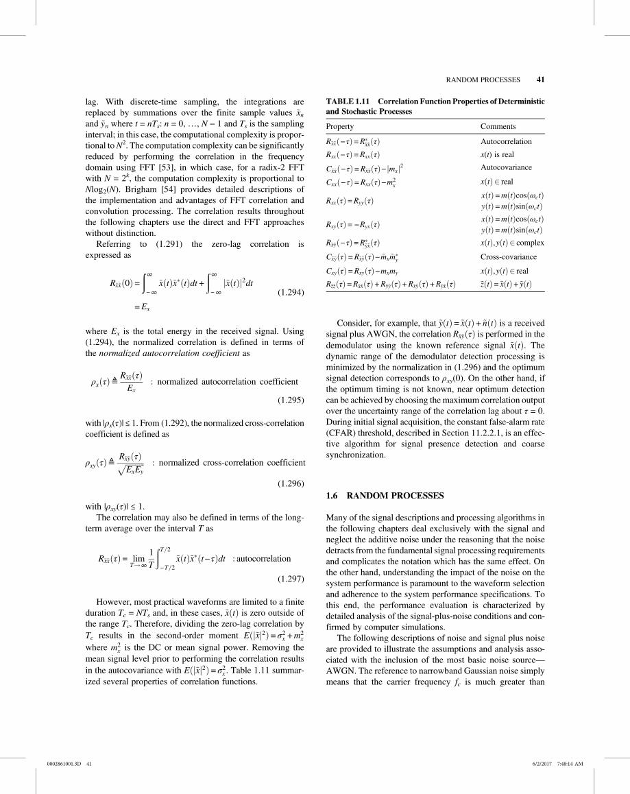
lag. With discrete-time sampling, the integrations arereplaced by summations over the finite sample values xnand yn where t = nTs: n = 0, …, N − 1 and Ts is the samplinginterval; in this case, the computational complexity is propor-tional toN2. The computation complexity can be significantlyreduced by performing the correlation in the frequencydomain using FFT [53], in which case, for a radix-2 FFTwith N = 2k, the computation complexity is proportional toNlog2(N). Brigham [54] provides detailed descriptions ofthe implementation and advantages of FFT correlation andconvolution processing. The correlation results throughoutthe following chapters use the direct and FFT approacheswithout distinction.

Referring to (1.291) the zero-lag correlation isexpressed as

Rxx 0 =∞

−∞x t x∗ t dt +

∞

−∞x t 2dt

=Ex

(1.294)

where Ex is the total energy in the received signal. Using(1.294), the normalized correlation is defined in terms ofthe normalized autocorrelation coefficient as

ρx τ ≜Rxx τ

Exnormalized autocorrelation coefficient

(1.295)

with |ρx(τ)| ≤ 1. From (1.292), the normalized cross-correlationcoefficient is defined as

ρxy τ ≜Rxy τ

ExEynormalized cross-correlation coefficient

(1.296)

with |ρxy(τ)| ≤ 1.The correlation may also be defined in terms of the long-

term average over the interval T as

Rxx τ = limT ∞

1T

T 2

−T 2x t x∗ t−τ dt autocorrelation

(1.297)

However, most practical waveforms are limited to a finiteduration Tc = NTs and, in these cases, x t is zero outside ofthe range Tc. Therefore, dividing the zero-lag correlation byTc results in the second-order moment E x 2 = σ2x +m

2x

where m2x is the DC or mean signal power. Removing the

mean signal level prior to performing the correlation resultsin the autocovariance with E x 2 = σ2x . Table 1.11 summar-ized several properties of correlation functions.

Consider, for example, that y t = x t + n t is a receivedsignal plus AWGN, the correlation Rxy τ is performed in thedemodulator using the known reference signal x t . Thedynamic range of the demodulator detection processing isminimized by the normalization in (1.296) and the optimumsignal detection corresponds to ρxy(0). On the other hand, ifthe optimum timing is not known, near optimum detectioncan be achieved by choosing the maximum correlation outputover the uncertainty range of the correlation lag about τ = 0.During initial signal acquisition, the constant false-alarm rate(CFAR) threshold, described in Section 11.2.2.1, is an effec-tive algorithm for signal presence detection and coarsesynchronization.

1.6 RANDOM PROCESSES

Many of the signal descriptions and processing algorithms inthe following chapters deal exclusively with the signal andneglect the additive noise under the reasoning that the noisedetracts from the fundamental signal processing requirementsand complicates the notation which has the same effect. Onthe other hand, understanding the impact of the noise on thesystem performance is paramount to the waveform selectionand adherence to the system performance specifications. Tothis end, the performance evaluation is characterized bydetailed analysis of the signal-plus-noise conditions and con-firmed by computer simulations.

The following descriptions of noise and signal plus noiseare provided to illustrate the assumptions and analysis asso-ciated with the inclusion of the most basic noise source—AWGN. The reference to narrowband Gaussian noise simplymeans that the carrier frequency fc is much greater than

TABLE 1.11 Correlation Function Properties of Deterministicand Stochastic Processes

Property Comments

Rxx −τ =R∗xx τ Autocorrelation

Rxx −τ =Rxx τ x(t) is real

Cxx −τ =Rxx τ − mx2 Autocovariance

Cxx −τ =Rxx τ −m2x x t real

Rxx τ =Ryy τx t =m t cos ωcty t =m t sin ωct

Rxy τ = −Ryx τx t =m t cos ωcty t =m t sin ωct

Rxy −τ =R∗yx τ x t ,y t complex

Cxy τ =Rxy τ −mxm∗y Cross-covariance

Cxy τ =Rxy τ −mxmy x t ,y t real

Rzz τ =Rxx τ +Ryy τ +Rxy τ +Ryx τ z t = x t + y t

0002861001.3D 41 6/2/2017 7:48:14 AM

RANDOM PROCESSES 41

the signal modulation Nyquist bandwidth BN so that the 2fcheterodyning or homodyne mixing terms are completelyeliminated through filtering. In such cases, the white noisein the baseband demodulator bandwidth is denoted by thesingle-sided noise density No watts/Hz, where single-sidedrefers to positive frequencies.

1.6.1 Stochastic Processes

The subject of stochastic processes is discussed in consider-able detail by Papoulis [55] and Davenport and Root [56] andthe following definitions are often stated or implied in theapplications discussed in throughout the following chapters.A stochastic process is defined as a random variable that is afunction of time and the random events χ in S as depicted inFigure 1.14. In this context the random variable is character-ized as x(t,χ). For a fixed value of t = ti, x(ti,χ) is a randomvariable and χ = χi, x(t,χi) denotes as the real random processx(t) such that x(ti) is a random variable with pdf fX(x:ti); ingeneral, the pdf of x(t) is defined as fX(x:t).

1.6.1.1 Stationarity There are several ways to define thestationarity of a stochastic process, for example, stationarityof finite order, asymptotic stationary, and periodic stationar-ity; however, the following two are the most frequentlyencountered.

Strict-Sense Stationary Process The stochastic process x(t)is strict-sense stationary, or simply stationary, if the statisticsare unaltered by a shift in the time axis. Furthermore, two ran-dom variables are jointly stationary if the joint statistics areunaltered by an equal time shift of each random variable, thatis, the probability density function f(x ; t) is the same for alltime shifts τ. This is characterized as

f x1,x2,…; t1, t2,… = f x1,x2,…; t1 + τ, t2 + τ,…

1 298

Wide-Sense Stationary Process The stochastic process x(t)is wide-sense stationary (WSS) if its expected value is con-stant and autocorrelation function is a function of the timeshift τ = t2 − t1 t1 and t2. WSS stationarity is characterizedas

E x t =mx = constant 1 299

and

E x t x t−τ =Rx τ (1.300)

Because wide-sense stationarity depends on only the firstand second moments it is also referred to asweak stationarity.A function of two random processes is wide-sense stationary

if each process is wide-sense stationary and their cross-correlation function is dependent only the time shift, that is,

E x t1 y t2 =Rxy t1− t2 =Rxy τ (1.301)

1.6.1.2 Ergodic Random Process The random process x(t), defined earlier, is an ergodic random process if the statis-tics of x(t) are completely defined by the statistics of x(t,χ).Denoting the random process x(ti,χ) as an ensemble of x(t,χ), then ergodicity ensures that the statistics x(ti) are iden-tical to those of the ensemble; in short, the time statistics areidentical to the ensemble statistics.* Ergodicity of the mean,of the stochastic process x(t,χ), exists under the condition

x t,χ i =E x ti,χ i (1.302)

where the time average is defined as

x t,χi ≜ limT ∞

12T

T

−Tx t,χi dt (1.303)

and the ensemble average is defined as

E x ti,χ ≜∞

−∞χfχ ti,χ dχ (1.304)

Since the mean value of a random process must be a con-stant, the ergodic of the mean theorem states that the equalitycondition in (1.302) is satisfied when E x ti,χ = η iwhere η is a constant. This is a nontrivial task to prove, how-ever, following the discussion by Papoulis [57], the ergodicof the mean theorem states that

limT ∞

12T

T

−Tx t dt =E x t = η

iff limT ∞

12T

T

−TRx τ dτ = η2

(1.305)

The iff condition in (1.305) is formally expressed in termsof the autocovariance function for which the limit T ∞is expressed as the variance σ2x = η

2−E x t 2. However,from (1.305), the expectation E[x(t)] = η resulting in σ2x = 0.Therefore, the limit T ∞ of the autocovariance functionconverges in probability with the conclusion thatE x t,χi =E x ti,χ proving ergodicity of the mean.† Dem-onstration of ergodicity of the autocorrelation function

*Papoulis (Reference 8, Chapter 9) discusses the ergodicity of a stochasticprocess with respect to certain parameters.†Convergence in probability is also discussed by Davenport and Root(Reference 6, pp. 66–71).

0002861001.3D 42 6/2/2017 7:48:14 AM


is considerably more involved, requiring the fourth-ordermoments.

1.6.2 Narrowband Gaussian Noise

Consider the noise described by the narrowband process [58]with bandwidth B << fc expressed as

n t =N t cos ωct + θ t −N t sin ωct + θ t (1.306)

where N(t) and θ(t) represent, respectively, the envelopand phase of the noise and ωc = 2πfc is the angular carrierfrequency. Upon expanding the trigonometric functions,(1.306) can also be expressed as

n t = nc t cos ωct −ns t sin ωct (1.307)

where

nc t =N t cos θ t (1.308)

and

ns t =N t sin θ t (1.309)

The noise terms nc(t) and ns(t) are uncorrelated with spec-trum S(f) and bandwidth B, such that S(f) = 0 for |f − fc| > B/2.This is the general characterization of a narrowband noiseprocess; however, in the following analysis, nc(t) and ns(t)are also considered to be statistically independent, stationaryzero-mean white noise Gaussian processes with one-sidedspectral density No watts/Hz.

Because of the stationarity, the noise autocorrelation isdependent only on the correlation lag τ and is evaluated as

Rnn τ =E n t n t−τ

=E nc t cos ωct −ns t sin ωct

nc t−τ cos ωc t−τ −ns t−τ sin ωc t−τ

(1.310)

Upon evaluating the product in (1.310) and distributingthe expectation, it is found that the conditions for stationarityrequire* Rss(τ) = Rcc(τ) and Rcs(τ) = −Rsc(τ) so that (1.310)reduces to

Rnn τ =Rcc τ cos ωcτ −Rss τ sin ωcτ (1.311)

The noise power is evaluated using (1.311) with τ = 0 withthe result Rnn(0) = Rcc(0) = σ2n. This evaluation can be carried

further using the Wiener–Khinchin theorem† which statesthat the power spectral density of a WSS random processis the Fourier transform of the autocorrelation function,that is,

Sn f =∞

−∞Rnn τ e− j2πf τdτ (1.312)

From (1.312) the inverse Fourier transform is

Rnn τ =∞

−∞Sn f ej2πf τdf (1.313)

and, substituting the condition that the single-sided noisespectral density is defined as No watts/Hz, (1.313) becomes

Rn τ =No

2

∞

−∞ej2πf τdf =

No

2δ τ (1.314)

In (1.314) the single-sided noise density is divided by twobecause of the two-sided integration, that is, the integrationincludes negative frequencies. In this case, the noise power,defined for τ = 0, is infinite, however, when the ideal band-limited filter, with bandwidth B, is considered the noisepower in the filter centered at fc is computed as

Rn 0 =No

fc+B 2

fc −B 2df =NoB (1.315)

In this case the one-sided noise density No is used insteadof No/2 because the one-sided integration is over positivefrequencies.

If a linear filter with impulse response h(t) is used, the fre-quency response is given by

H f =∞

−∞h t e− j2πftdt (1.316)

The corresponding unit gain normalizing factor is |H(0)|.With the stationary noise process n(t) applied to the input ofthe filter, the output is determined using the convolution inte-gral and the result is as follows:

no t =∞

−∞n t−λ h λ dλ (1.317)

*See Problem 29.

†Leon-Garcia (Reference 29, p. 404) refers to this theorem as the Einstein–Wiener–Khinchin theorem based on the discovery of an earlier paper byAlbert Einstein.

0002861001.3D 43 6/2/2017 7:48:15 AM

RANDOM PROCESSES 43

Using (1.317) it can be shown (see Problem 33) thatthe normalized spectrum of the output noise is expressed,in terms of the input noise PSD Sn(f), as

Sno f = Sn fH f

H 0

2

(1.318)

where |H(0)| is the normalizing gain of the filter. Using(1.318), with Sn(f) = No/2 corresponding to white noise, theoutput noise power is evaluated as

Rno 0 =fc+B 2

fc−B 2Sn f

H f 2

H fc2df

=No

2

fc+B 2

fc −B 2

H f 2

H fc2df

=NoBn

(1.319)

where the second integral in (1.319) is recognized as the def-inition of the noise bandwidth of the bandpass filter with low-pass bandwidth Bn.

1.7 THE MATCHED FILTER

The problem in the detection of weak signals in noise is oneof deciding whether the detection filter output is due to thesignal and noise or simply noise only. The matched filter[59, 60], provides for the optimum signal detection in AWGNnoise based on the maximum instantaneous signal-to-noiseratio when sampled at the optimum time.* The matched filter,for an AWGN channel, is characterized as having an impulseresponse equal to the delayed time-reverse replica of thereceived signal. To maximize the signal detection probabilitythe matched filter output must be sampled at To as defined inthe following analysis. The matched filter can be implemen-ted at a convenient receiver IF or in the demodulator usingquadrature baseband-matched filters.

Considering the received signal, sr(t), the matched filterimpulse response depicted in Figure 1.28 is expressed as

h t =Gsr To− t (1.320)

The gain G is selected for convenience; however, it mustbe a constant value. The delay To is required to result in acausal impulse response, that is, the response of h(t ≤ 0) =0 for h(t) to be realizable; consequently, sr(t ≥ To) must bezero. Usually the selection of To is not an issue since manysymbol modulation functions are time limited or can be trun-cated without a significant impact on the transmitted signal

spectrum; however, the matched filter delay results in athroughput delay. To the extent that the impulse approxi-mates (1.320) a detection loss will be encountered.

The criterion of the matched filter is to provide the max-imum signal-to-noise ratio in the AWGN channel whensampled at the optimum time To. The following matched fil-ter analysis follows that of Skolnik [61]. The signal-to-noiseratio of interest is

γf =sr t 2

max

N(1.321)

where sr t 2max = sr To 2 is evaluated as

so To2 =

∞

−∞S f H f ej2πfTodf

2

(1.322)

and N is the noise power evaluated as

N =∞

−∞N f H f 2df =

No

2

∞

−∞H f 2df (1.323)

In these expressions, the filter spectrum H(f) is normal-ized, such thatH(0) = 1, and the last equality in (1.323) resultsbecause the channel noise is white with one-sided constantpower density of No watts/Hz. Substituting (1.322) and(1.323) into (1.321) results in the expression for the signal-to-noise ratio

γf =

∞


No 2∞

−∞H f 2df

2

(1.324)

Themaximum signal-to-noise ratio is evaluated by applyingSchwarz’s inequality (see Section 1.14.5, Equation 5) to thenumerator of (1.324). Upon substituting f ∗ f = S f ej2πfTo

and g f =H f into the Schwarz inequality, (1.324) isexpressed as

0

0 To

Tot

sr(t)

t

h(t)

FIGURE 1.28 Example received signal and correspondingmatched filter.

*The matched filter was first derived by D.O. North [59] and is also referredto as the North filter.

0002861001.3D 44 6/2/2017 7:48:15 AM


γf ≤

∞

−∞S f 2df

∞

−∞H f 2df

No 2∞

−∞H f 2df

=

∞

−∞S f 2df

No 2

(1.325)

The equality condition of the signal-to-noise ratio in(1.325) applies when f(f) = cg(f), where c > 0 is a conven-iently selected constant resulting in the matched filter fre-quency response expressed as

H f =GS∗ f e− j2πfTo matched filter frequency response

(1.326)

where G = 1/c is an arbitrarily selected constant gain greaterthat zero. Upon applying Parseval’s theorem and recognizingthat the numerator of the second equality in (1.325) is the sig-nal energy, E, the optimally sampled matched filter outputsignal-to-noise ratio is simply expressed as

γf max =2ENo

baseband modulated signal (1.327)

Therefore, for the AWGN channel, the optimally sampledmatched filter output results in a signal-to-noise ratio that is afunction the signal energy and noise density and is independ-ent of the shape of the signal waveform. The factor of two in(1.327) results from the analytic or baseband signal descrip-tion in the derivation of the matched filter. Typically, thereceived signal spectrum is modulated onto a carrier fre-quency with an average power equal to one-half the peak car-rier power. In this case, the signal-to-noise ratio at the outputof the matched filter is one-half of that in (1.327) resulting in

γf max =E

Nocarrier moduated signal (1.328)

Referring to (1.326), the inverse Fourier transform of thecomplex conjugate of the signal spectrum results in the filterimpulse response corresponding to the time reverse of the sig-nal. In addition, the inverse Fourier transform of the exponen-tial function in (1.326) results in a signal time delay of Toseconds, so the resulting filter impulse response, h(t), corre-sponds to the example depicted in Figure 1.28. Consequently,the matched filter impulse response can be expressed in thetime domain by (1.320) or in the frequency domain by (1.326).

The detection loss associated with a filter that is notmatched to the received signal is evaluated as

ρf ≜γf

γf max=

so t 2max No

2E No(1.329)

where so t and No are the output signal and mean noisepower density at the output of the unmatched filter. Typically

the matched filter is based on the transmitted waveform;however, the received signal into the matched filter may bedistorted by the channel or receiver filtering* resulting in adetection loss. The matched filter implementation may alsoresult in design compromises that result in a detection loss.

1.7.1 Example Application of Matched Filtering

In this example, a BPSK-modulated received signal is con-sidered with binary source data bits bi = {0,1} expressedas the unipolar data di = (1 − 2bi) = {1,−1} over the data inter-vals iT ≤ t ≤ i+ 1 T of the bit duration T. The received signalplus noise is expressed as

r t = dis t + n t (1.330)

The signal is described as

s t =Acos ωct (1.331)

The noise is zero-mean additive white Gaussian noise withone-sided spectral density No described as

n t = nc t cos ωct −ns t sin ωct (1.332)

The receiver-matched filter impulse response and Fouriertransform are given by

h t =As To− tℑ

H f =GS∗ f e− j2πfTo (1.333)

In (1.333) the signal spectrum defined as S(f) and thesquared magnitude of the matched filter output at the opti-mum sampling point is

so To2 =

∞


=∞

−∞S f 2df =E

(1.334)

where the gain G = |H(0)| is normalized to one resulting in aunit gain-matched filter response H(f).

Referring to the additive noise described by (1.332) andSection 1.6.2, the noise power at the output of the matchedfilter is expressed as

Rno 0 =No

2

B 2

−B 2H f 2df (1.335)

where B/2 is the baseband bandwidth of the matched filter.

*Adaptive channel equalizers are often used to compensate for the channeldistortion.

0002861001.3D 45 6/2/2017 7:48:16 AM

THE MATCHED FILTER 45

The received signal, as expressed in (1.330), can berewritten in terms of the optimally sampled matched filteroutput as

l r iTo = Edi +No

2ni (1.336)

where ni are iid zero-mean, unit variance, white Gaussian

noise samples. Upon dividing (1.336) by No 2 the sampledmatched filter output is expressed as

l ri =2ENo

di + ni (1.337)

The sampled values l(r(iTo)) and l (ri) are referred to assufficient statistics, in that, they contain all of the informationin r(t), expressed in (1.330), to make a maximum-likelihood

estimate di of the source-bit di. The normalized form in(1.337) is used as the turbo decoder input discussed inSection 8.12. In Section 1.8 the sufficient statistic is seento be a direct consequence of the log-likelihood ratio.

1.7.2 Equivalence between Matched Filteringand Correlation

Consider the receiver input as the sum of the transmittedsignal plus noise expressed as

r t = s t + n t (1.338)

The cross-correlation of r(t) with a replica of the receivedsignal is computed as

R τ =∞

−∞r t s t−τ dt cross-correlation (1.339)

Defining the matched filter impulse response as h(t), thematched filter output response to the input r(t) is

yo t =∞

−∞r λ h t−λ dλ convolution (1.340)

However, referring to the preceding matched filter discus-sion, the matched filter response is equal to the delayed imageof the signal, such that,

h t = s To− t (1.341)

As mentioned previously, the delay To ensures thatthe filter response is causal and, therefore, realizable.To substitute (1.341) into (1.340) first let t = t−λ so thath t−λ = s To− t−λ = s λ− t−To and substitute thisresult in (1.340) to get

yo t =∞

−∞r λ h t−λ dλ

=∞

−∞r λ s λ− t−To dλ

=R t−To

(1.342)

So that the convolution response is equal to the cross-correlation response delayed by To. If the input noise is zero,so that r(t) = s(t), the same conclusion can be drawn regardingthe autocorrelation response.

1.8 THE LIKELIHOOD ANDLOG-LIKELIHOOD RATIOS

Bayes criterion is based on two events, referred to as hypoth-esis H1 and H0, that are dependent upon a priori probabilitiesP1 and P0 and the, respective, associated costs (C01,C11) and(C10,C00). Letting m correspond to the decision and n corre-spond to the hypothesis, the range of the cost is 0 ≤ Cmn ≤ 1with Cmn + Cnn|m n = 1. The cost of a correct decision is Cnn

and an incorrect decision is Cmn|m n. For communicationlinks the cost of incorrect decision is typically higher thana correct decision so that Cmn|m n > Cnn. For example, whenCmn|m n = 1 and Cnn = 0 the decision threshold minimizesthe probability of error which is the goal of communicationdemodulators. In summary,

Cmn =m= n cost of correct decision

m n cost of decision error(1.343)

and the a priori probabilities are typically known and equal.In the following example, the hypotheses correspond to

selecting di = {1,−1}, such that, under the two hypotheses

H1 di = + 1 with a prioi probability P1

H0 di = −1 with a prioi probability P0(1.344)

with the observations

ri = di + ni t = iTo (1.345)

corresponding to the optimally sampled outputs of thematched filter. In terms of the a priori, the transition probabil-ities, and the cost functions, the hypothesis H1: with di = 1 ischosen if the following inequality holds,

Pr H1r H1 P1 C01−C11 ≥Pr H0

r H0 P0 C10−C00

(1.346)

0002861001.3D 46 6/2/2017 7:48:16 AM


otherwise, chose H0 with di = −1. The decisions are madeexplicit under the following rearrangement of (1.346)

Pr H1r H1

Pr H0r H0

>H1

<H0

P0 C10−C00

P1 C01−C11(1.347)

Left and right sides of (1.347) are defined as the likelihoodratio (LR) Λ(r) and decision threshold η or, alternately, as thelog-likelihood ratio (LLR) lnΛ(r) with the threshold lnη, so(1.347) is also expressed as

Λ r >H1

<H0

η or lnΛ r ><H0

H1lnη alternate decisions thresholds

(1.348)

1.8.1 Example of Likelihood and Log-LikelihoodRatio Detection

Consider the two hypotheses H1 and H0 mentioned earlierwith di = {1,−1} and the observation ri in (1.345) with theadditive noise ni characterized as iid zero-mean whiteGaussian noise, denoted as N(0,σn). The transition probabil-ities are expressed in terms of the Gaussian noise pdf as

p n =1

2πσne− r−m 2 2σ2n (1.349)

Upon forming the likelihood ratio and recognizing thatm = ±di, the likelihood ratio decision simplifies to

exp2riσ2n

>H1

<H0

P0 C10−C00

P1 C01−C11(1.350)

and the log-likelihood ratio decision simplifies to

2σ2n

ri >H1

<H0

lnP0 C10−C00

P1 C01−C11(1.351)

Recognizing that l(ri) is a sufficient statistic, (1.351) isrewritten as

l ri >H1

<H0

σ2n2ln

P0 C10−C00

P1 C01−C11(1.352)

When C10 = C01 = 1, C00 = C11 = 0, and P0 = P1 the LLRsimplifies to

l ri >H1

<H0

0 ln η= 1 = 0 (1.353)

Therefore, the data estimate is di = 1 when l(ri) > 0, other-

wise, di = −1. Recall that observations ri : t = iTo are made atthe output of the matched filter. These concepts involving theLR and LLR surface again in Section 3.2 and the notion of thenatural logarithm of the transitions probabilities is discussedin the following section involving parameter estimation.

1.9 PARAMETER ESTIMATION

The subject of optimum signal detection in noise was exam-ined in the preceding section in terms of a pulsed-modulatedcarrier and it resurfaces throughout the following chapters inthe context of a number of different waveform modulations.However, signal detection is principally based on the signalenergy without regard to specific signal parameters, althoughfrequency and range delay must be estimated to some degreeto declare signal presence and subsequently detection. Signaldetection uses concepts involving direct probabilities,whereas the subject of parameter estimation uses conceptsinvolving inverse probabilities as discussed by Feller [32],Slepian [62], Woodward and Davies [63], and others. Thedistinction between these concepts is that direct probabilityis based on the probability of an event happening, whereasinverse probability formulates the best estimate of an eventthat has already occurred. With this distinction, it is evidentthat parameter estimation involves inverse probabilities. Themajor characteristic of inverse probability is the use of apriori information associated with the available knowledgeof each source event. At the receiver the a posteriori proba-bility is expressed in terms of the inverse probability usingBayes rule that associates the transition probability and apriori knowledge of the source events.

The subject of this section is signal parameter estimationand, although the major parameter of interest in communica-tions is the estimation of the source information, the estima-tion of parameters like, frequency, delay, and signal andnoise powers are important parameters that aid in the estima-tion of the source information. For example, estimation ofthe received signal and noise powers form the basis for esti-mating the receiver signal-to-noise ratio that is used in thenetwork management to improve and maintain communica-tion reliability. Furthermore, characterizing the theoreticallimits in the parameter estimates provides a bench mark ortarget for the accuracy of the parameter estimation duringthe system design.

The following discussion of statistical parameter estima-tion is largely based on the work of Cramér [64], Rao [65],Van Trees [66], and Cook and Bernfeld [67]. The receivedsignal is expressed in terms of the transmitted signal withM unknown parameters a1, a2, …, aM and additive noise, as

r t = s t;a1,a2,…,aM + n t (1.354)

0002861001.3D 47 6/2/2017 7:48:17 AM

PARAMETER ESTIMATION 47

Considering that N discrete samples of the received signaland additive noise are used to estimate the parameters, thejoint probability density function (pdf) of the samples is

pr r1,r2,…,rN a1,a2,…,aM = pn r1−s1,r2−s2,…,rN −sN(1.355)

where the noise samples ni = ri − si are substituted intothe joint pdf of the noise. The noise samples are statisticallyindependent and the statistical characteristics of the noiseare assumed to be known. Therefore, based on the receivedsignal-plus-noise samples ri, the receiver must determinethe estimates â1, â2,…, âM of the M unknown parameters.The probability density function pr(r1,… |a1,…) in (1.355)is called the likelihood function.

Van Trees discusses several estimation criteria* and thefollowing focuses on the optimum estimates for the mean-square (MS) error† and maximum a posteriori probability(MAP) criterion that are defined, respectively, for a singleparameter a as

ams r =∞

−∞apa r a r da MS estimate (1.356)

and

∂

∂alnpa r a r

a= amap r

= 0 MAP equation (1.357)

The estimate âms(r) is optimum in the sense that it resultsin the minimumMS error over all si and a. TheMAP estimateâmap(r) is the solution to (1.357) and is optimum in the sensethat it locates the maximum of the a posteriori probabilitydensity function; however, the solution must be checked todetermine if it corresponds to the global maximum in theevent of a multimodal distribution.

By applying Bayes rule to (1.357), the MAP estimate isexpressed in terms of the a priori pdf, pa(a), and the likelihoodfunction, pr a r a , as

∂

∂alnpr a r a +

∂

∂alnpa a

a = amap r

= 0 (1.358)

When the a priori probabilities are unknown, that is, asthe a priori knowledge approaches zero, (1.358) becomesthe maximum-likelihood equation and âml(r) is themaximum-likelihood estimate, evaluated as the solution to

∂

∂alnpr a r a

a = aml r= 0 ML estimate (1.359)

To make use of these estimates it is necessary to determinethe bias and the variance of the estimate. The mean value ofthe estimate is computed as

E a r =∞

−∞a r pr a r a dr (1.360)

The bias of the estimate is defined as B a =E a r −a. If,as indicated, the bias is a function of a, the estimate has anunknown bias, however, if the bias is B, independent of a,the estimate has a known bias that can be removed fromthe observation measurements r. In general, for any knownbiased estimate â(r) of the real random variable a, the vari-ance is defined as

σ2a =Var a r −a ≜E a r −a 2 −B2 (1.361)

Although the bias and variance are often difficult to deter-mine, the Cramér–Rao inequality provides a lower bound onthe variance of the estimate. For a biased estimate of the ran-dom parameter a with a priori pdf pa(a), the variance is lowerbounded by the Cramér–Rao inequality [64, 66]

σ2a ≥∂E a r ∂a 2

E∂ln pr a r a

∂a+∂ln pa a

∂a

2 biased; variable

(1.362)

or, the equivalent result,

σ2a ≥∂E a r ∂a 2

−E∂2 ln pr a r a

∂a2+∂2 ln pa a

∂a2

biased; variable

(1.363)

When the estimate is unbiased, that is, when E a r = a,the estimation variance of the random variable a simplifies to

σ2a ≥1

E∂ln pr a r a

∂a+∂ln pa a

∂a

2

unbiased; variable

(1.364)

or, the equivalent result,

σ2a ≥1

−E∂2 ln pr a r a

∂a2+∂2 ln pa a

∂a2

unbiased; variable

(1.365)

*The criteria are based on Bayes estimation procedure that minimizes the riskassociated with the cost or weight assigned to various kinds of statistical deci-sions. In communication systems, the decision costs are assigned tominimizethe demodulator bit-error probability.†The MS error is also referred to as the minimum mean-squareerror (MMSE).

0002861001.3D 48 6/2/2017 7:48:17 AM


The Cramér–Rao bound in these relationships is formu-lated in terms of the Schwarz inequality and the equalitycondition applies when

∂ln pr a r a

∂a+∂ln pa a

∂a= k a r −a

MAP efficient estimate condition

(1.366)

where k is a constant. Therefore, (1.366) guarantees that theequality condition for the variance applies in (1.362) through(1.365); in this case, the MAP estimate is defined as an effi-cient estimate. Furthermore, an unbiased estimate, excludingthe trivial case k = 0, requires that a r = a leading to (1.358).

When the a priori knowledge pa(a) is constant, that is,the parameter a is nonrandom, or unknown, then (1.359)also requires that a = a or aml r = a. Under the maximum-likelihood (ML) criteria Schwarz’s equality conditionapplies when

∂ln pr a r a

∂a= k a a r −a

ML efficient estimate condition

(1.367)

In this case, the constant k(a) may be a function of a; thiscondition only applies when parameter a is a constant whichcorresponds to the ML estimate.

Van Trees lists three principles based on the forgoingresults:

1 The mean-square (MS) error estimate is always themean of the a posteriori density, that is, the conditionalmean.

2 The MAP estimate corresponds to the value of a forwhich the a posteriori density is maximum.

3 For a large class of cost functions, the optimum esti-mate is the conditional mean whenever the a posterioridensity is a unimodal function which is symmetricabout the conditional mean. The Gaussian pdf is a com-monly encountered example.

By way of review, the estimates are evaluated using the aposteriori pdf; however, if the parameter is a random variable,the a posteriori pdf must be expressed in terms of the transi-tion distribution and the a priori pdf of the random parameterusing Bayes rule. If the estimate is unbiased, that is, ifB=E a r −a = 0, evaluation of the Cramér–Rao boundsimplifies to (1.364); it is sometimes necessary to use theequivalent expression in (1.365). The Cramér–Rao equalitycondition is established if the left-hand side of (1.366) canbe expressed in terms of the right-hand side where k is aconstant parameter resulting from Schwarz’s condition forequality.

If the a priori knowledge is unknown then the maximum-likelihood equation given in (1.359) is used to determinemaximum-likelihood estimate. In this case, the Cramér–Rao bound is established by omitting the dependence ofpa(a) in, (1.362) through (1.365) and the equality conditionis established if the left-hand side of (1.367) can be expressedin terms of the right-hand side where, in this case, the con-stant k(a) is a function of the parameter a. With either theMAP or ML estimates, if the bias is zero and the equalitycondition applies, the estimate is referred to as an efficientestimate.

Van Trees shows that for the MS estimate to be an effi-cient estimate, the a posteriori probability density pa r a rmust be Gaussian for all r and, for efficient MAP estimates,ams r = amap r . However, it may be easier to solve the MAPequation than to determine the conditional mean as requiredby the MS estimation procedure.

1.9.1 Example of MS and MAP ParameterEstimation

As an example application of the parameter estimation pro-cedures discussed earlier, consider the Poisson distributionthat is used to predict population growth, telephone call ori-ginations, gamma ray emissions from radioactive materials,and is central in the development of queueing theory [68].For this example, the Poisson distribution is characterized as

pa a n =an

ne−a a ≥ 0; n = 0,1,2,… (1.368)

In the application of (1.368) to queueing theory, a = λt isthe average number of people entering a queueing line inthe time interval 0 to t and λ is the arrival rate. The aposteriori distribution pa n a n is the probability of a condi-tioned on exactly n arrivals occurring in the time interval.A fundamental relationship in the Poisson distribution is thatthe time interval between people entering the queueing line isexponentially distributed and is characterized by the a prioridistribution

pa a = e−a a ≥ 0 (1.369)

The a posteriori pdf in (1.368) is expressed in terms of thea priori and transition pdfs as

pa n a n =pn a n a pa a

pn n=k

nane−2a (1.370)

where the constant k is a normalizing constant that includes 1/pn(n). Integrating of the second equality in (1.370) withrespect to da over the range 0 to∞ and setting the result equalto one, the value of k is found to be k = 2n+1 and (1.370)becomes

0002861001.3D 49 6/2/2017 7:48:18 AM


pa n a n =2n+ 1

nane−2a (1.371)

Using (1.356) and (1.371) the MS estimate is evaluated as

ams n =2n+ 1

n

∞

0an + 1e−2ada=

n

2(1.372)

Also, using (1.357) and (1.371) the MAP estimate is eval-uated as

∂

∂aln

2n+ 1

nane−2a =

∂

∂aln

2n+ 1

n+ n ln a −2a

=n

a−2

a= amap n= 0

(1.373)

and solving the second equality in (1.373) for a results inamap n = n 2. As is typical in many cases, the MS andMAP estimation procedures result in the same estimate. Itis left as an exercise (see Problem 38) to determine the biasof the estimates, compute the Cramér–Rao bound, and using(1.366), determine if the estimates are efficient, that is, if theCramér–Rao equality condition applies.

1.9.2 Constant-Parameter Estimation inGaussian Noise

To simplify the description of the estimation processing,the analysis in this section considers the single constant-parameter case with zero-mean narrowband additiveGaussian noise. Under these conditions, the estimation isbased on the solution to the maximum-likelihood equationwith the joint pdf of the received signal and noise written as

pr r1,r2,…,rN ;a = pn r1−s1,r2−s2,…,rN −sN

=N

i= 1

pn ri−si(1.374)

where a is the constant parameter to be estimated and ri = si +ni represents the received signal samples. The sampling ratesatisfies the Nyquist sampling frequency and the secondequality in (1.374) recognizes that the noise samples are inde-pendent. The following analysis is based on the work of theWoodard [24] and Skolnik [61] and uses the maximum-likelihood estimate of (1.359) with the Cramér–Rao boundexpressed by (1.365).

Using (1.374) with zero-mean AWGN, the minimumCramér–Rao bound on the variance of the estimate isexpressed as

σa2 min = −E∂2

∂a2ln

N

i

1

2πσnexp −

ri−si2

2 σ2n

−1

= −E∂2

∂a2ln kexp

−12No

N

i= 1

ri−si2Δt

−1

= −E∂2

∂a2ln kexp

−12No

Te

0r t −s t 2dt

−1

(1.375)

In arriving at the third equality in (1.375) the factor k isindependent of the parameter a and, it is recognized that,σ2n =NoB where B = 1/Te is the bandwidth corresponding tothe estimation time. The integral is formed by letting Δt0 as the number of samples N ∞ over the estimation inter-val Te. Upon taking the logarithm of the product kexp(−) andperforming the partial derivatives on the integrand, (1.375)simplifies to

σa2 min =E−1No

Te

0r t −s t

∂2s t

∂a2−

∂s t

∂a

2

dt

−1

=1No

Te

0

∂s t

∂a

2

dt

−1

(1.376)

The last equality in (1.376) is the basis for determining thevariance and is obtained by moving the expectation inside ofthe integral and recognizing that E r t −s t =E n t = 0.The following example outlines the procedures for estimatingthe variance of the estimate using the ML procedures.

1.9.2.1 Example of ML Estimate Variance EvaluationConsider the signal s(t) expressed as

s t =Acos ωot +ωt2 2 +ϕ (1.377)

where A is the peak carrier voltage, ωo is the IF angular fre-quency, ω is the angular frequency rate, and ϕ is a constantphase angle; the signal power is defined Ps = A2/2.

The variance of the frequency estimate is determined bysquaring the partial derivative of s(t) respect to ωo and inte-grating over the estimation interval Te as indicated in (1.376).Under these conditions the analysis of the Cramér–Rao lowerbound is performed as follows.

σ2ωomin =

A2

No

Te

0t2sin2 ωot +ωt

2 2 +ϕ dt−1

=Ps

No

Te

0t2 1−cos 2ωot +ωt

2 + 2ϕ dt−1

(1.378)

0002861001.3D 50 6/2/2017 7:48:18 AM


Upon neglecting the term involving 2ωo and performingthe integration, (1.378) becomes

σ2ωomin =

3T2e γe

rad2 s2 (1.379)

where γe = PsTe/No is the signal-to-noise ratio in the estima-tion bandwidth of 1/Te. In terms of the carrier frequency foin hertz, the standard deviation of the estimate is

σf o min =3

2πTe γeHz (1.380)

In a similar manner, the standard deviation of the fre-quency rate and phase are evaluated as

σfmin =

5π T2

e γeHz s (1.381)

and

σϕ min =1γe

rad (1.382)

The evaluation of the standard deviation of the signalamplitude (A) estimation error is left as an exercise (seeProblem 39).

1.9.3 Received Signal Delay and FrequencyEstimation Errors

Accurate estimation of the signal delay and frequency areessential in aiding the signal acquisition processing by mini-mizing the overall time and frequency search ranges. The delayestimation accuracy (σTd) is inversely related to the signalbandwidth (B) and the signal frequency estimation accuracy(σfd) is inversely related to the time duration (T) of the signal.Neglecting the signal-to-noise dependence of each measure-ment, these inverse dependencies are evident, in that, the prod-uct σTdσfd 1/TB where TB is the time-bandwidth productof the waveform. For typical modulated waveforms T and Bare inversely related so that simultaneous accurate time andfrequency estimates are not attainable. However, the use ofspread-spectrum (SS) waveformmodulation provides for arbi-trarily large BT products with simultaneous accurate estimatesof Td and fd. The analysis of delay and frequency estimationerrors in the following sections is based on the work ofSkolnik [61] and can be applied to conventional or SS-modulated waveforms. In Section 1.9.3.3 delay and frequencyestimation is examined using a DSSS-modulated waveform.

1.9.3.1 Delay Estimation Error Based on EffectiveBandwidth The signal delay measurement accuracy using

the effective signal bandwidth was introduced by Gabor[69] and is discussed by Woodward [24] and defined as thestandard deviation of the delay measurement expressed as*

σTd =1

β 2γesecond (1.383)

where γe = Ps/NoW = E/No is the signal-to-noise ratio† meas-

ured in the two-sided bandwidth W, No is the one-sidednoise density, Ps is the signal power, and β is the effectivebandwidth of the signal. β2 is the normalized second momentof the waveform spectrum |S(f)|2, defined as

β2 ≜

∞

−∞2πf 2 S f 2df

∞

−∞S f 2df

(1.384)

The denominator in (1.384) is the signal energy and theintegration limits extend over the frequency range f ≤ |W/2|corresponding to the nonzero signal spectrum. The one-way range error corresponding to (1.383) is σrng = cσTdmeters where c is the free-space velocity of light in meter/second.

For the rectangular symbol modulation function rect(t/T), band limited to W Hz with β2 W/T and large time-bandwidth products WT/2, (1.383) is evaluated as

σTd =T

WTγeband-limited rect t T symbol; WT 2 1

(1.385)

1.9.3.2 Frequency Estimation Error Based on EffectiveSignal Duration In a manner similar to the analysis ofthe delay estimation error in the preceding section, Manasse[70] shows that the, minimum root-mean-square (rms) errorin the frequency estimate is given by‡

σfd =1

α 2γeHz (1.386)

where γe = E/No is the signal-to-noise ratio measured in thetwo-sided bandwidthW, No is the one-sided noise density, Ps

is the signal power, and α is the effective time duration of the

*Woodward refers to the delay error as the standard deviation of the error.Slepian’s analysis [62] is based on the likelihood function and also arrivesat (1.383).†The factor of two in γe results because No is the one-sided noise density andW is the two-sided bandwidth.‡The notation σfd is used to denote the standard deviation of the frequencyestimation error.

0002861001.3D 51 6/2/2017 7:48:19 AM


received signal. The parameter α2 is the normalized secondmoment of the waveform s(t) and is defined as

α2 ≜

∞

−∞2π t 2s2 t dt

∞

−∞s2 t dt

(1.387)

The Doppler frequency results from the velocity (v) andthe carrier frequency (fc) and is expressed as fd = (v/c)fc.Frequency errors resulting from hardware oscillators areusually treated separately and combined as the root-sum-square (RSS) of the respective standard deviations.

For the band-limited rect(t/T) symbol modulation usedin the preceding section, the normalized second moment isevaluated as α2 (πT)2/3 and (1.386) is expressed as

σfd =3

πT 2γeband-limited rect t T symbol; WT 2 1

(1.388)

Comparison of (1.385) and (1.388) demonstrates theinverse relationship between the estimation accuracy of therange-delay and frequency errors for conventional (unspread)modulations. For example, for a given time bandwidth (WT)product and signal-to-noise ratio (γe), the delay estimate errordecreases with decreasing symbol duration; however, the fre-quency estimate error increases. The issue resolves about thesignal-to-noise ratio in the estimation bandwidth. For exam-ple, with conventional waveform modulations,WT = 2BT = 2so BT = 1 and the bandwidth changes inversely with the sym-bol duration. Consequently, by decreasing symbol duration,the bandwidth increases resulting in a signal-to-noise γs,

measured in the symbol bandwidth, degradation of B/Bwhere B >B. Therefore, in the previous example, to maintaina constant signal-to-noise ratio γe the estimation intervalmust be appropriately adjusted. As mentioned previously,the solution to simultaneously obtaining accurate estimatesof range delay and frequency while maintaining a constantγs, involves the use of a SS-modulated signals with an inher-ently largeWT product as discussed in the following section.

1.9.3.3 Improved Frequency and Time Estimation ErrorsUsing the DSSS Waveform The DSSS waveform uses apseudo-noise (PN) sequence of chips with and instantaneousbandwidth (W) over the estimation interval (T) as shown inFigure 1.29.* The resulting largeWT product signal providesfor arbitrarily low time and frequency estimation errors. Thisis accomplished by the respective selection of a high band-width (short duration) chip interval (τ) and the low bandwidth(long duration) estimation interval T. The estimation intervalcan be increased to improve the frequency estimate; con-versely, the chip interval can be decreased to improve therange-delay estimate; however, to maintain the accuracy ofthe other, the number of chips per estimation interval (N)must be increased. These relationships are described in termsof the pulse compression ratio, defined as ρ = T/τ = N. InFigure 1.29 the chips are depicted as appropriately delayedAdnrect((t−n)/τ − 0.5): n = 0,…,N − 1 functions and, becauseof the equivalence between the correlator and matched filter,the peak correlator output is a triangular function with a peakvalue† of AN. When sampled at t = Nτ, the correlator output

AT

f

S(f)

–2/τ –1/τ 1/τ 2/τ0

(b)

Signal spectrum

TimeSidelobes

Nτ

(c)

Demodulator correlation response

Rs(t)

t

AN

A

Transmitted signal

dn = {1,–1}

2τ 3τ Nττ0

s(t)

t. . . . . .

. . .

. . .

T

}dn

(a)

FIGURE 1.29 Time–frequency estimation using DSSS waveform.

*Although not shown in the figure, the chips are ± binary pulses which sug-gest that the received signal carrier frequency is BPSK modulated.†This suggests that the local reference is an identical unit amplitude PNsequence that is synchronized with the received PN sequence.

0002861001.3D 52 6/2/2017 7:48:19 AM


results in the maximum signal-to-noise ratio measured in thebandwidth of 1/T Hz.

Based on the fundamental principles for jointly achievingaccurate time and frequency estimates as stated earlier, thetriangular shape of the wide bandwidth correlator output isrelated to the accuracy of the time estimate and the low band-width sampled output at interval of T = Nτ determines theaccuracy of the frequency estimate. Therefore, evaluationof the time and frequency estimation accuracies of the DSSSwaveform involves evaluating, respectively, the effectivebandwidth (β) of the triangular function and the effectivetime duration (α) of the rect(t/T − 0.5) function.

Delay Estimation Error of the DSSS Waveform The delayestimation error is based on detecting the changes in the lead-ing and trailing edge of wideband signals. This does notrequire that the signal has a short duration but that the band-width is sufficiently wide to preserve the rapid rise and falltimes of the correlator response. On the other hand, receivedsignals with additive noise must be detected and the para-meters estimated under the optimum signal-to-noise condi-tions as provided by matched filtering or correlation. Inthis regard, the correlator output in Figure 1.29 is examinedin the context of the signal delay estimate error.

The triangular function, corresponding to the correlatoroutput, is an isosceles triangle with base and height equalto 2τ and AN, respectively, and is described as

Rs ξ =AN 1− ξ τ ξ ≤ τ (1.389)

where, for convenience, ξ = t − Nτ such that the time axisis shifted so that the isosceles triangle is symmetrical aboutξ = 0. The effective bandwidth of Rs(ξ) is evaluated (seeProblem 41) as

β =3τ

triangular function (1.390)

and the corresponding standard deviation of the delay esti-mate is

σTd =τ

3 2γetriangular function (1.391)

Frequency Estimation Error of the DSSS Waveform Thefrequency estimation error is based on the interval T of thePN sequence under the conditions corresponding to the localPN reference being exactly synchronized with and multipliedby the received signal; in other words, with zero frequencyand phase errors, the integrand of the correlation integral isconstant over the interval T. However, with a frequency errorof fε Hz the correlator response is computed as

Rs T ; fε =AT

0ej2π fεξdξ

=ATejπ fεTsin π fεT

π fεTcorrelator response with fε

1 392

The principal frequency error in the main lobe of the sinc(fεT) function corresponds to| fε| ≤ 1/T which defines the fun-damental resolution accuracy of the frequency estimate.However, the effective duration of the correlator of lengthT = Nτ is evaluated (see Problem 42) as

α=2πT3

rectangular function (1.393)

and the corresponding standard deviation of the frequencyestimate is

σfd =3

2πT 2γerectangular function (1.394)

Considering the SS pulse compression ratio, or processinggain, ρ = T/τ, the correlator output signal-to-noise ratio (γe) in(1.391) and (1.394) is measured in the bandwidth of 1/T. Theproduct of the estimation accuracies of the SS waveform is

σTdσfd =τ

2πTγe=

12πργe

(1.395)

Therefore, the time and frequency estimates accuraciescan be made arbitrarily low, even in low signal-to-noise ratioenvironments, by designing a SS waveform with a suffi-ciently high pulse compression ratio.

1.9.3.4 Effective Bandwidth of SRRC and SRCWaveforms In view of the increasing demands on band-width, the spectral containment of the spectral raised-cosine (SRC) waveform meets the corresponding need forspectrum conservation. Although the spectral root-raised-cosine (SRRC) waveform has a slightly wider bandwidththan the SRC waveform, it is preferred because of theimproved matched filter detection* and, in the context ofrange delay estimation, provides for a somewhat better rangedelay estimate. The spectrum of the SRC waveform is char-acterized, in the context of a spectral windowing function, inSection 1.11.4.1 and the spectrum of the SRRC is character-ized in Section 4.3.2 in the context of the optimum transmit-ted waveform for root-raised-cosine (RRC) waveformmodulation. The following analysis compares the effective

*The optimally sampled SRRC matched filter output results in the maximumsignal energy and orthogonal symbol samples resulting in zero intersymbolinterference.

0002861001.3D 53 6/2/2017 7:48:19 AM


bandwidth of the SRC and SRRC waveforms with the under-standing that the SRC delay estimate is based on the matchedfilter out samples taken symmetrically about the optimummatched filter sample at t = To.

The dependence of the effective bandwidth of the SRRCand SRC waveforms on the excess bandwidth parameter α isexpressed as

βT = π13+

π2−8π2

α2 SRRC waveform (1.396)

and

βT = π4−3α+ 12α2−α3

3 4−α−8α2 16−α

2π 2 4−αSRC waveform

(1.397)

Equations (1.396) and (1.397) are plotted in Figure 1.30that demonstrates the advantages of the wider bandwidthSRRC waveform in providing short rise-times symbols withthe associated improvement in range-delay detection. In thisregard, the rect(t/T) modulated received symbol, as character-ized by the BPSK-modulated waveform, has zero rise-timeand results in perfect range-delay detection in a noise-freechannel and receiver; however, infinite bandwidth is requiredto achieve this performance. The dashed curve in Figure 1.30shows the normalized effective bandwidth of the rect(t/T)modulated symbol after passing through an ideal (1/B)rect(f/B) filter with one-sided bandwidth B/2 Hz; this is referredto a filtered BPSK and is discussed in the following section.

The noise bandwidth of the SRRC frequency functionis significant, in that, it corresponds to the demodulator-matched filter response used in the detection of the SRRC-modulated waveform. On the other hand, the interest in thenoise bandwidth of the SRC is more academic in naturebecause of its application as a windowing function. In eitherevent, the noise bandwidth of the SRRC and SRC frequencyfunctions is examined in Problem 44.

1.9.3.5 Effective Bandwidth of the Ideally Filtered rect(t/T) Waveform In this case the effective bandwidth ofthe ideal symbol modulation, characterized by rect(t/T), isevaluated after passing through an ideal filter with frequencyresponse (1/B)rect(f/B) where B/2 is the one-sided or low-pass bandwidth of the filter. The filter response is examinedin Section 1.3 and the normalized effective bandwidth of thefiltered symbol is characterized by Skolnik [71] as

βT =πBT −sin πBT

Si πBT + cos πBT −1 πBT

ideally filtered rect t T waveform

(1.398)

This result is plotted in Figure 1.31 as a function of BTwhere T is the symbol duration. From this plot it is evidentthat as BT approaches infinity the standard deviation of therange-delay estimate approaches zero resulting in an exactestimate of the true range delay. A practical application isto define a finite bandwidth which is sufficiently wide soas not to degrade the symbol detection through intersymbolinterference.

Defining the excess bandwidth factor for the ideal filter asα =B Rs =BT , where Rs = 1/T is the rect(t/T) symbol rate, in

Ideal filter time-bandwidth product (BT)0 2 4 6 8 10 12 14 16 18 20

0

1

2

3

4

5

6

7

Nor

mal

ized

eff

ectiv

e ba

ndw

idth

(βT

)

FIGURE 1.31 Normalized effective bandwidth for filteredrect(t/T) waveform.

RC excess bandwidth factor (α)0.0 0.2 0.4 0.6 0.8 1.0

Nor

mal

ized

eff

ectiv

e ba

ndw

idth

(βT

)

0.8

1.0

1.2

1.4

1.6

1.8

2.0

2.2

2.4

BPSK time bandwidth product (BT)

0.5 0.6 0.7 0.8 0.9 1.0

SRRC

SRC

FilteredBPSK

FIGURE 1.30 Normalized effective bandwidths for SRRC andSRC waveforms.

0002861001.3D 54 6/2/2017 7:48:20 AM


terms of the excess bandwidth factor α of the raised-cosine(RC) waveform, α = 1+ α 2. The corresponding range ofBT is 1/2 ≤ BT ≤ 1; this range of the filtered rect(t/T) effectivebandwidth from Figure 1.31 is plotted as the dashed curve inFigure 1.30. The range of BT results in significant intersym-bol interference and received symbol energy loss even underthe ideal conditions of symbol time and frequency correction.However, under the same conditions, if the SRRC waveformand matched filter responses are sufficiently long, the inter-symbol interference and symbol energy loss will be negligi-ble. At the maximum SRRC normalized effective bandwidthof βT = 2.27, the filter time bandwidth product corresponds toBT = 2.64 or a 32% increase with the filter bandwidth span-ning the main signal spectral lobe and 16% of the adjacentsidelobes. In other words, the one-sided filter bandwidthspans 1.32 lobes and, referring to Appendix A, this resultsin a performance loss of about 1.25 dB for BPSK waveformmodulation; for a loss of less than 0.3 dB the BT productshould be greater than 5 with a resulting effective bandwidthof βT = 3.23 corresponding to a (3.23/2.27 − 1)100 = 42%improvement relative to the best SRRC range-delay estima-tion error; however, the required bandwidth is 150% wider.The bandwidth and range-delay estimation accuracy aredesign trade-off in the waveform selection.

1.10 MODEM CONFIGURATIONS ANDAUTOMATIC REPEAT REQUEST

The three basic modulator and demodulator configurationsare simplex, half-duplex, and full-duplex. The definition ofsimplex communications involves communication in onedirection between a modulator/transmitter and a remotereceiver/demodulator. Examples of simplex communicationsinclude broadcasting from radio and television stations orfrom various types of monitoring devices. Half-duplex com-munications is a broader definition including two-way com-munications but only in one direction at a time. In thesecases, transceivers and modems are required at each loca-tion. A common application of half-duplex operation is thepush-to-talk handheld radios. Full-duplex communicationsprovide the capability to communicate in both directionssimultaneously. In these cases the bidirectional communica-tions may use identical transceivers and modems operating atthe same symbol rate; however, as is often the case, the com-munication link in one direction may be designated as thereverse channel and operated at a lower symbol rate. In eitherevent, the forward and reverse channels must operate atdifferent, noninterfering, frequencies.

The transfer of data is often performed using informationframes or packets, each containing a cyclic redundancy check(CRC) code for error checking. If an error is detected thereceiving terminal requests that the frame be retransmitted,otherwise an acknowledgment may be returned indicating

that the frame was received without error. These protocolsare referred to as automatic repeat request [72] (ARQ). TheARQ protocol requires either a half-duplex or full-duplexcommunication capability. The two commonly used varia-tions of the ARQ protocol are generally referred to as idle-repeat request (RQ) and continuous-RQ.* However, morecomplex variations involving point-to-point and multipointprotocols are also defined.†

The remainder of this section analyzes the idle-RQ proto-col which is the simplest ARQ system to implement and eval-uate, in that, when a data frame is transmitted a timer isinitiated and a new frame is transmitted only after acknowl-edgment (ACK) that the current frame was received withouterrors and/or the timer has not exceeded a maximum timeoutTmax. However, the current frame is retransmitted if thetimer exceeds Tmax, a negative acknowledgment (NAK) isreceived, indicating the receipt of an incorrect frame, or theACK or NAK code is received in error. The timer limit isbased on the information bits per frame, the bits in theACK and NAK codes, the date rates, and the expectedtwo-way link propagation delay through the media. Theidle-RQ implementation also has the advantage of requiringless data storage compared to the continuous-RQ protocoland the Go-back-N protocol [73]. However, the performancecost of these advantages is that the end-to-end transmissionefficiency is lower and more sensitive to the link propagationdelay. The end-to-end transmission efficiency is defined as

ηtrans ≜Rbf

Rbf(1.399)

where Rbf is the average bit rate over the forward channel andRbf is the uninterrupted forward channel bit rate.

The idle-RQ is modeled as shown in Figure 1.32 with thedelays and other parameters defined in Table 1.12.

Using the parameters described earlier, the average timeassociated with the transmission and acknowledgment isdescribed as

T =N Tdf + Tsf + 2Tp + Tcs + Tdr + Tsr + Tcp (1.400)

where N is the average number of frame repetition based onthe specified bit-error probability and the number of frameinformation and CRC bits NB. The computation of N is basedon iid additive white Gaussian channel noise over all of theNB bits. This provides for the probability of a correct messageto be expressed in terms of the discrete binomial distribution‡

given the bit-error probability Pbef; the result is expressed as

*Reference 72, Chapter 4, Protocol Basics.†Reference 72, Chapter 5, Data Link Control Protocols.‡See Table 1.42.

0002861001.3D 55 6/2/2017 7:48:20 AM

MODEM CONFIGURATIONS AND AUTOMATIC REPEAT REQUEST 55

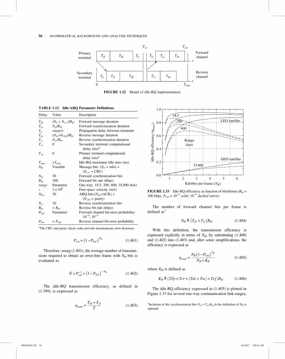
Pcm = 1−PbefNB (1.401)

Therefore, using (1.401), the average number of transmis-sions required to obtain an error-free frame with NB bits isevaluated as

N =P−1cm = 1−Pbef

−NB (1.402)

The idle-RQ transmission efficiency, as defined in(1.399), is expressed as

ηtrans =Tdf + Tsf

T(1.403)

The number of forward channel bits per frame isdefined as∗

NB ≜ Tdf + Tsf Rbf (1.404)

With this definition, the transmission efficiency isexpressed explicitly in terms of NB, by substituting (1.400)and (1.402) into (1.403) and, after some simplifications, theefficiency is expressed as

ηtrans =NB 1−Pbef

NB

NB +KB(1.405)

where KB is defined as

KB ≜ 2Tp+ Tcr + Tdr +Tsc +Tcf Rbf (1.406)

The idle-RQ efficiency expressed in (1.405) is plotted inFigure 1.33 for several one-way communication link ranges;

0

Tdf

t

Tcs

Tp

Primaryterminal

Secondaryterminal

Tp Tp

Tcp

tTmin

Tsf

TdfTsf TdrTsr

TdrTsr

Forwardchannel

Reversechannel

FIGURE 1.32 Model of idle-RQ implementation.

TABLE 1.12 Idle-ARQ Parameter Definitions

Delay Value Description

Tdf (Nb + Ncrc)/Rbf Forward message durationTsf Nsf/Rbf Forward synchronization durationTp range/c Propagation delay between terminalsTdr (Nbr+Nchk)/Rbr Reverse message durationTsr Nsr/Rbr Reverse synchronization durationTcs 0 Secondary terminal computational

delay (ms)a

Tcp 0 Primary terminal computationaldelay (ms)a

Tmax >Tmin Idle-RQ maximum idle time (ms)NB Variable Message bits: (Nb = info) +

(Ncrc = CRC)Nsf 30 Forward synchronization bitsRbf 100 Forward bit rate (kbps)range Parameter One-way: 18.5, 200, 600, 35,800 (km)c 3 × 108 Free-space velocity (m/s)Nbrt 30 ARQ bits:(Nbr=ACK) +

(Nchk = parity)Nsr 10 Reverse synchronization bitsRbr = Rbf Reverse bit rate (kbps)Pbef Parameter Forward channel bit-error probability:

10−4, 10−5

Pber = Pbef Reverse channel bit-error probability

aThe CRC and parity check codes provide instantaneous error decisions.

Kilobits-per-frame (NB)61 2 3 4 5

Idle

-RQ

eff

icie

ncy

(ηtr

ans)

0.0

0.2

0.4

0.6

0.8

1.0

GEO satellite

LEO satellite200

18.5

Range(km)

600

35 800

FIGURE 1.33 Idle-RQ efficiency as function of bits/frame (Rbf =100 kbps, Pbef = 10−5 solid, 10−4 dashed curve).

∗Inclusion of the synchronization bits Nsf = Tsf Rbf in the definition of NB isoptional.

0002861001.3D 56 6/2/2017 7:48:21 AM


the solid curves correspond to Pbef = 10−5 and the dashedcurves correspond to Pbef =10

−4. The impact of the link prop-agation delay (Tp) is significant and results in long idletimes for the ACK/NAK response. The performance is alsodependent on the link bit-error probabilities, the bit rate,and the number of bits per frame.

The optimum number of forward channel bits per frame,NB, corresponding to the maximum efficiency, ηtrans(max), isevaluated by differentiating (1.405) with respect to NB andsetting the result equal to zero and then solving for NB(opt).Following this procedure, the optimum NB, corresponding tothe maximum efficiency, is evaluated as the solution to thequadratic equation

N2B +NBKB−KB λ = 0 (1.407)

where λ = ln 1 1−Pbe . The solution to (1.407) is

NB opt = −KB

2+

KB

2

2

+KB

λ(1.408)

Using the example parameters, NB(opt) is listed inTable 1.13 for the conditions shown in Figure 1.33.

Optimizing the message frame size using NB(opt) has lim-ited practical appeal because the resulting maximum effi-ciency may be unacceptable or because of the broad rangeof NB over which the slope around ηtrans(max) is virtuallyunchanged; this latter point is seen in Figure 1.33 correspond-ing to Pbef = 10−5. Selecting NB from a range that satisfies anacceptable minimum transmission efficiency is a preferablecriterion and operating at low bit-error probabilities offersa wider range of selections.

1.11 WINDOWS

Windows have been characterized and documented by anumber of researchers [74, 75], and this section focuses onthe windows that are used in the simulation codes in the fol-lowing chapters to enhance various performance objectives.Windows are applied in radar and communication systems to

achieve a variety of objectives including antenna sidelobereduction, improvements in range resolution and target dis-crimination, spectral control for adjacent channel interference(ACI) reduction [76], ISI control, design of linear phase fil-ters, and improvements in parameter estimation algorithms.Windows can be applied as time or frequency functions toachieve complementary results depending on the application.

Windows are described in terms of the discrete-time sam-ples* w(n) where n is indexed over the finite window lengthof N samples. When the window is applied as a discrete-frequency sampled window the notation W(n) is used. Thediscrete-time sampled rectangular window, defined, forexample, as w(n) = 1 for |n| ≤ N/2 and zero otherwise, istypically used as the reference window by which the perfor-mance measures of other windows are compared. The spec-trum of the time-domain rectangular window is described interms of the sinc(x) function as S(f) = sinc(nf/N). The rectan-gular window is also referred to as a uniformly weighted orsimply as an unweighted window.

Several window parameters [75] that are useful in select-ing a window for a particular application are the gain, thenoise bandwidth, and the scalloping loss. The window volt-age gain is defined as

Gv ≜n

w n (1.409)

The noise bandwidth of the window follows directlyfrom the definition of the noise bandwidth defined byEquation (1.46). In terms of the discrete-time sampling andapplication of Parseval’s theorem, the normalized noisebandwidth is expressed as

Bn =nw2 n

nw n

2 (1.410)

In terms of Hertz, the bandwidth is given by

Bn Hz =Bn

Tw(1.411)

where 1/TwHz is the fundamental frequency resolution of thewindow with duration Tw seconds. The theoretical normal-ized noise bandwidth of the rectangular window is Bn = 1,so the noise bandwidth is Bn = 1/Tw Hz. Harris [75] definesthe scalloping loss (SL) of a time-domain window, as the fre-quency domain loss, relative to the maximum level, mid-waybetween two maximum adjacent DFT outputs. The scallop-ing loss is expressed as

TABLE 1.13 Optimum NBa Corresponding to the Maximum

Efficiency Conditions in Figure 1.33

Pbef

Range (km)

18.5 200 600 35,800

1e−3 204 338 478 9601e−4 697 1,232 1,889 7,5891e−5 2,261 4,077 6,416 38,3801e−6 7,208 13,079 20,757 143,1251e−7 22,850 41,546 66,112 477,137

aNB in bits.

*The notation w(n) is a time-normalized sample corresponding to w(nTs)where Ts is the sampling interval. Similarly, the frequency-domain samplesW(n) are normalized by fs/N = 1/NTs.

0002861001.3D 57 6/2/2017 7:48:22 AM

WINDOWS 57

SL≜W π N

W 0=

nw n e− jπn N

nw n

(1.412)

The characteristics of the various windows considered inthe following sections are summarized in Tables 1.14 and1.15. The maximum sidelobes correspond to those adjacentto the central, or main, lobe, and apply to the time (or fre-quency) domains depending on whether the window isapplied, respectively, in the frequency (or time) domains.The scalloping loss results from the frequency or timedomain ripple resulting from contiguous repetitions of thewindow functions. Harris has compiled an extensive tableof windows and their performance characteristics.

The duration of the window and the manner in which it issampled is dependent upon the application. In the followingdescriptions, the sampling is applied to windows that are sym-metrical and asymmetrical about t = 0 as described by (1.413)using the rect(x) window. The rect(x) window is a uniformlyweighted window* that is used to describe the window delay†

and duration Tw for all arbitrarily weighted windows.

w t =

rectt−Td

Tw−m−

12

asymmetrcial about t = 0

rectt−TdTw

−m symmetrical about t = 0

(1.413)

The parameter Td introduces a delay and m is an integercorresponding to a contiguous sequence of windows; in thefollowing analysis Td and m are zero. Considering N to bean integer number of samples over the window duration with

the sampling interval of Ts = Tw/N seconds, the windows arecharacterized, with a maximum value of unity, in terms of thesample index n. In the following examples, the Bartlett ortriangular window‡ is used and the respective odd and evenvalues of N are 9 and 8. For odd integers N, the asymmetricaltriangle window is expressed as

w n N odd = 1−n− N−1 2

N−1 20 ≤ n ≤N−1, asymmetrical

(1.414)

and the symmetrical triangle window is expressed as

w n N odd = 1−n

N−1 2n ≤ N−1 2, symmetrical

(1.415)

For the even integers, the asymmetrical triangle window isexpressed as

w nN evenn = n + 5

=

2n + 1N

0 ≤ n <N 2

2−2n + 1N

N 2 ≤ n ≤N−1

, asymmetrical

(1.416)

and the symmetrical triangle window is expressed as

w n N evenn= n + 5

=1 +

1−2 n

N−N 2 ≤ n < 0

1−1 + 2 n

N0 ≤ n ≤N 2−1

, symmetrical

(1.417)

Equations (1.414) through (1.417) are plotted inFigure 1.34 with the circles indicating the window samplinginstances. The distinction between the symmetrical andasymmetrical sampling is evident and must be applied com-mensurately to the sampled data. In this regard, the windowscan be applied, for example, to the transmitted data-modulated symbols for spectrum control, to the received datasymbol for detection, or to the FFT window for spectrumevaluation. With minimum shift keying (MSK) modulation,discussed in Section 4.2.3.4, a cosine window is applied toeach quadrature rail that are delayed, or offset, by one-halfsymbol period, so the notion of symmetrical and asymmetri-cal windows applies.§ The examples using an odd number ofwindow samples, shown in Figure 1.34a and b, include thefirst and last window samples that are zero and increase

TABLE 1.14 Summary of Window Performance Results

WindowMax.Sidelobe (dB) At ±fTw

Scalloping Loss (dB)with Tw Zero-Padding

0 1 2 3

Rectangular −13.26 1.5 3.92 0.91 0.4 0.18Bartlett −26.4 3.0 1.81 0.44 0.20 0.09Blackman −58.2 3.6 1.09 0.27 0.12 0.05Blackman–

Harris−92.0 4.52 0.82 0.20 0.09 0.04

Hamming −42.6 4.5 1.74 0.43 0.19 0.09Cosine k = 1 −23.0 1.89 2.08 0.51 0.22 0.10

k = 2 −31.5 2.4 1.41 0.35 0.15 0.07k = 3 −39.3 2.83 1.06 0.26 0.12 0.05k = 4 −46.7 3.33 0.85 0.21 0.09 0.04

Using N = 200 samples/window.

*Since the weighting is constant over Tw, the uniformly weighed window isalso referred to as an unweighted window.†The application of a window to a sequence of received symbols prior tospectral analysis requires the window to be appropriately delayed.

‡The triangular window is used to emphasize the sampling with respect to anonuniformly weighted window.§Windows applied to transmitter symbols for spectral control are generallyreferred to as symbol shaping functions and denoted as p(t).

0002861001.3D 58 6/2/2017 7:48:22 AM


–4 –3 –2 –1 0 1 2 3 4

Nor

mal

ized

am

plitu

de

0.00

0.25

0.50

0.75

1.00

Sample (n)

(a)

Nodd = 9: symmetrical

Sample (n)0 1 2 3 4 5 6 7 8

Nor

mal

ized

am

plitu

de

0.00

0.25

0.50

0.75

1.00

(b)

Nodd = 9: asymmetrical

–4 –3 –2 –1 0 1 2 3 4

Nor

mal

ized

am

plitu

de

0.00

0.25

0.50

0.75

1.00

Sample (n')

(c)

Neven = 8: symmetrical

Sample (n')0 1 2 3 4 5 6 7 8

Nor

mal

ized

am

plitu

de

0.00

0.25

0.50

0.75

1.00

(d)

Neven = 8: asymmetrical

FIGURE 1.34 Examples of triangular window sampling.

TABLE 1.15 Summary of Window Performance Results

Bartlett Blackman Blackman–Harris Hamming

Samples (N) Bn Gv Bn Gv Bn Gv Bn Gv

1000 1.3357 0.4995 1.728 0.4196 2.006 0.3584 1.364 0.5395500 1.335 0.499 1.730 0.419 2.008 0.358 1.365 0.539200 1.340 0.498 1.735 0.418 2.014 0.357 1.368 0.538100 1.347 0.495 1.744 0.416 2.025 0.355 1.373 0.53550 1.361 0.490 1.762 0.412 2.045 0.352 1.383 0.53125 1.394 0.480 1.799 0.403 2.088 0.344 1.403 0.52212 1.467 0.455 1.884 0.385 2.186 0.329 1.450 0.502

Cosine k = 1 Cosine k = 2 Cosine k = 3 Cosine k = 4

1000 1.235 0.636 1.502 0.4995 1.737 0.424 1.946 0.3746500 1.236 0.635 1.503 0.499 1.738 0.4236 1.948 0.3742200 1.240 0.633 1.507 0.498 1.744 0.422 1.954 0.373100 1.246 0.630 1.515 0.495 1.752 0.420 1.964 0.37150 1.260 0.624 1.531 0.490 1.770 0.416 1.984 0.36825 1.290 0.610 1.562 0.480 1.807 0.407 2.026 0.36012 1.364 0.580 1.636 0.458 1.892 0.389 2.121 0.344

Noise bandwidth and voltage gain.

0002861001.3D 59 6/2/2017 7:48:23 AM

WINDOWS 59

symmetrically to the peak value. Although these cases arevisually appealing, the sampled windows in Figure 1.34cand d use an even number of samples per window and resultin same performance commensurate with the Nyquist sam-pling rate. Furthermore, using an even number of samplesis suitable for analysis using the efficient FFT.

The case for using an even number of samples can bemade based on the down-sampled output of a high samplerate analog-to-digital converter. For example, relative to areceived data-modulated symbol, the down-sampled, orrate-reduced, output is the average symbol amplitude ofthe down-sampled interval from nTs to (n + 1)Ts, so thewindow weighting should be applied to the point mid-way between the two samples as is often done using rectan-gular integration. This is accommodated by the even num-ber of samples over the window interval shown inFigure 1.34c and d, with the understanding that the datasample at n = n + 0.5 results from the linear interpolationof the data between sample n and n + 1. In addition toapplying the correctly aligned window with interpolateddata samples, this sampling arrangement also removesthe delay estimation bias thereby improving the symboltracking performance. Of course, the roles of the odd andeven sampling can be reversed; however, it is convenientto use an even number of samples per symbol into thedetection-matched filter for symbol tracking and the detec-tion of quadrature symbol offset modulations. However, aslong the Nyquist sampling criterion is satisfied the symbolinformation can be extracted in either case. In the followingsections, the spectrums of the various windows are evalu-ated using both symmetrically and asymmetrically sampledwindows with an odd number of samples. The reason forthis choice is simply based on esthetics or eye appeal whichis particularly noticeable when only a few number of sam-ples is used.

1.11.1 Rectangular Window

In the time domain, the rectangular window is a uniformlyweighted function described by the rect(t/Tw) functionwith amplitude equal to unity over the range |t/Tw| ≤ 1/2and zero otherwise. Expressing the time in terms of thediscrete samples t = nTs, where Ts is the sampling interval,results in the sample range |n| ≤ (N − 1)/2 for the symmetricalwindow and 0 ≤ n ≤N − 1 for the asymmetrical window,whereN = Tw/Ts is the total number of samples per window.

The spectrum of the rectangular window is described interms of the sinc(fTw) function and, upon letting f = nδfand δf = Δf/L, where Δf = 1/Tw is the fundamental frequencyresolution of the window, the spectrum is expressed as

W n =sin πn L

πn L= sinc

n

L(1.418)

Defining the frequency increment in this way allows forL samples per spectral sidelobe. The Fourier transformsrelationship between the time and frequency domains is dis-cussed in Section 1.2. Special applications involving the rect(x) window in the time and frequency domains are discussedin Sections 1.11.4, 4.4.1, 4.4.4, and 4.4.5.

1.11.2 Bartlett (Triangular) Window

The sampling of the Bartlett or triangular window is dis-cussed earlier under a variety of conditions that dependlargely on the application and signal processing capabilities.The Bartlett window is shown in Figure 1.35 for N = 21 sam-ples per symbol. Considering the frequency dependence ofthe spectral attenuation, expressed as sinc2(fTw/2), the spec-tral folding about the Nyquist band fN = fs/2 = N/2Tw is neg-ligible for N = 201 and the peak spectral sidelobes arevirtually identical to the theoretical Bartlett spectrum overthe range of frequencies shown in Figure 1.36b, althoughthe sidelobe level at fTw = 29 is −65.8 dB and the theoreticalvalue is −66.5 dB. Furthermore, upon close examination, thepeak values of the sidelobe are progressively shifted to theright with increasing fTw. These observations are more evi-dent for the case involving N = 21 where the first sidelobelevel is −26.8 dB (1 dB higher that theory) and the sidelobeat fTw = 9 is significantly skewed to the right with a level 6 dBhigher than the theoretical value. The sidelobe skewing is adirect result of the odd symmetry of the folded spectrumabout 2kfTw : k = 1, 2, … which does not occur when N iseven. However, with even values of N, the sidelobes are stillaltered by the folded spectral sidelobes. This phenomenon isa direct result of the sampling and the implicit periodicity ofthe window when using the discrete Fourier transform. Theseobservations do not alter the utility of windows for spectralcontrol; however, they may influence the spectral detail inapplications involving spectral analysis.

Sample (n)

0 2 4 6 8 10 12 14 16 18 20

Win

dow

am

plitu

de

0.0

0.2

0.4

0.6

0.8

1.0

FIGURE 1.35 Bartlett window with N = 21 samples.

0002861001.3D 60 6/2/2017 7:48:23 AM


1.11.3 Cosine Window

The sidelobes of the window spectrum can be reduced byproviding additional shaping or tapering of the window func-tion at the expense of a wider main spectral lobe that resultsin a higher noise bandwidth. For example, the rectangularwindow has an abrupt change in amplitude leading to a firstsidelobe level of −13 dB, a spectral roll-off proportional to1/f 2 (6-dB/octave), and a noise bandwidth of 1/Tw Hz. Onthe other hand, the Bartlett window has an abrupt changein the slope of the amplitude leading to a first sidelobe levelof −26.9 dB, a spectral roll-off of 1/f 4 (12-dB/octave), and anoise bandwidth of 1.336/Tw. The cosine window results inthe k-th derivative of the amplitude, that is, the slope of theamplitude at the edges of the window is zero resulting in evengreater spectral sidelobe roll-off.

The cosine window is characterized as

w n = cosk ϕn + δ1 (1.419)

where δ1 = 0 when n ≤ N−1 2 and δ1 = −π/2 whenn = 0,…, N − 1; this corresponds to a sink(ϕn) window func-tion. The phase function in (1.419) is expressed as

ϕn =π

N−1n + δ0 n ≤ N−1 2 (1.420)

where δ0 = 0 when n odd and δ0 = 0.5 when n even.The cosine window is shown in Figure 1.37 for n > 0 and k =1, …,4. In the following subsections, the cosine windows forvarious values of k are described for the conditions δ0 = δ1 = 0.

The gain for the finite sampled cosine window with k = 1and N samples per window is given by

Gv =2π

N−1N

(1.421)

and the normalized noise bandwidth is given by

Bn =π2

8N

N−1(1.422)

Gv and Bn are recorded in Table 1.15 for various values of N.Equations (1.421) and (1.422) approach their theoretical lim-its as N ∞.

1.11.3.1 Cosine Window (k = 1) With k = 1 the cosinewindow is expressed as

w n = cos ϕn (1.423)

This window is used as the symbol weighting function forMSK modulation and, in terms of the window duration Tw,the theoretical spectrum is given by

0 2 4 6 8 10Nor

mal

ized

spe

ctru

m m

agni

tude

(dB

)

–60

–50

–40

–30

–20

–10

0

–25.9 dB

–40 dB

Normalized frequency (fTw)Normalized frequency (fTw)

0 2 4 6 8 1012141618202224262830Nor

mal

ized

spe

ctru

m m

agni

tude

(dB

)

–90

–80

–70

–60

–50

–40

–30

–20

–10

0

–26.9 dB

–46.0 dB

–65.8 dB

(a)

N = 21 samples

(b)

N = 201 samples

FIGURE 1.36 Bartlett (triangular) window spectrums.

Sample (n)0 2 4 6 8 10 12 14 16 18 20

Win

dow

am

plitu

de

0.0

0.2

0.4

0.6

0.8

1.0

k=

2

3

4

1

FIGURE 1.37 Cosine windows (δ0 = 0, δ1 = −π/2).

0002861001.3D 61 6/2/2017 7:48:24 AM

WINDOWS 61

W f =4Twπ

cos πfTw

1− 2fTw2 (1.424)

The spectrum shown in Figure 1.38a is based on computersimulation with N = 200 samples per window.

1.11.3.2 Cosine-Squared (Hanning)Window (k = 2) Thecosine-squared window with k = 2 is referred to as a Hanningwindow [74]. Applying trigonometric identities, this windowis expressed as

w n = 0 5 + 0 5cos 2ϕn (1.425)

and the spectrum is shown in Figure 1.38b for N = 200 sam-ples per window.

1.11.3.3 CosineWindow (k = 3 and 4) Applying trigono-metric identities, the cosine windows for k = 3 and 4 areexpressed as

w n = 0 75cos φn + 0 25cos 3φn k = 3 (1.426)

and

w n = 0 375 + 0 5cos 2ϕn + 0 125cos 4ϕn k = 4

(1.427)

The spectrums for these two cases are shown inFigure 1.38c.

1.11.4 Temporal Raised-Cosine (TRC) Window

The temporal raised-cosine (TRC) window applies a cosineshaping function symmetrically about each end of the

0 2 4 6 8 10 12 14 16 18 20

Nor

mal

ized

spe

ctru

m m

agni

tude

(dB

)

k = 1

Normalized frequency (fTw)



0 2 4 6 8 10 12 14 16 18 20Nor

mal

ized

spe

ctru

m m

agni

tude

(dB

)

–120–110–100–90–80–70–60–50–40–30–20–10

0

–120–110–100

–90–80–70–60–50–40–30–20–10

0

–120–110–100–90–80–70–60–50–40–30–20–10

0

k = 2

(a)

k = 1

(b)

k = 2: Raised cosine (Hanning)

0 2 4 6 8 10 12 14 16 18 20

Nor

mal

ized

spe

ctru

m m

agni

tude

(dB

)

k = 3

4

(c)

(k = 3 and 4)

FIGURE 1.38 Cosine window spectrums.

0002861001.3D 62 6/2/2017 7:48:25 AM


rectangular window function, rect(nΔt/Tw), as shown inFigure 1.39. In this case, the integer n corresponds to the sam-ples N over the interval Tw such that N = Tw/Δt.

The TRC window is expressed as

w n =1 n <

1−α2

12

1−sinπ

αn −

12

1−α2

≤ n ≤1 + α2

(1.428)

where n = t/Tw = nΔt/Tw is the normalized sample index andα is a design parameter limited to 0 ≤ α ≤ 1. The TRCwindowis applied to the phase function of PSK-modulated wave-forms in Sections 4.2.8 and 4.4.3.9 to improve the waveformspectral containment while maintaining a constant signalamplitude; in this application α is referred to as the excessphase factor.

Letting m = f/Tw, the spectrum of the TRC amplitude win-dow is evaluated as

W m =sin πm

πm

cos απm

1− 2αm 2 (1.429)

1.11.4.1 Spectral Raised-Cosine Window The raised-cosine window when applied in the frequency domain isreferred to as the spectral RC (SRC) window and the param-eter α is referred to as the excess bandwidth. With m = fTw,the SRC frequency response is expressed as

W m =Tw m <

1−α2

Tw2

1−sinπ

αm −

12

1−α2

≤ m ≤1 + α2

(1.430)

and upon letting n = t/Tw, the SRC impulse response is eval-uated as

w n =sin πn

πn

cos απn

1− 2αn 2 (1.431)

This response has indeterminate solutions of the form 0/0at n = 0 and 1/(2α) that are evaluated as w 0 = 1 and

w12α

=α

2sin

π

2α(1.432)

Using these results, (1.431) is plotted in Figure 1.40 forseveral values of the excess bandwidth factor. The SRRCwindow, associated with spectral shaping of a modulatedsymbol, is discussed in detail in Section 4.3.2. In this appli-cation the symbol duration is T = Tw and the transmittedsymbol and demodulator-matched filter spectrums have asquare-root RC, or simply root RC, frequency response of

W n . The matched filter output results in the SRC impulseresponse shown in Figure 1.40 with symbol spacing corre-sponding to integer values of n that results in zero ISIn 0. With an AWGN channel and optimum matched filter

sampling the demodulator performance corresponds to max-imum-likelihood detection.

1.11.5 Blackman Window

The Blackman window uses three terms to provide moretapering of the window at the expense of a narrower timeresponse and a wider noise bandwidth. The Blackmanwindow is expressed as

w n = 0 42−0 5cos ϕn + 0 08cos 2ϕn (1.433)

where the phase function in (1.433) is expressed as

ϕn =2πN−1

n 0 ≤ n ≤N−1

=2πN−1

n+ N 2 − N 2 ≤ n ≤ N 2

(1.434)

Sample (n)0 1 2 3 4 5 6 7 8

Res

pons

e am

plitu

de

–0.25

0.00

0.25

0.50

0.75

1.00

Curve alphaSolid 0.2

Dot-dash 0.3Dashed 0.4

FIGURE 1.40 Impulse response of SRC window.

1

1/2

nΔtTw/2–Tw/2 0

w(n)

FIGURE 1.39 Temporal raised-cosine window.

0002861001.3D 63 6/2/2017 7:48:25 AM

WINDOWS 63

This definition of the phase function results in a symmet-rical window for all values of N with indexing over ± N 2as shown in Figure 1.41a for N = 21. The spectrum of theBlackman window corresponding to N = 200 samples perwindow is shown in Figure 1.41b.

1.11.6 Blackman–Harris Window

The Blackman–Harris window is expressed as

w n = co−c1cos ϕn + c2 cos 2ϕn −c3 cos 3ϕn (1.435)

Harris [75] performed a gradient search on the coefficientsci to minimize spectral sidelobe level and the results are givenin Table 1.16 for a three- and four-term window.

The Blackman–Harris window, as formulated byHarris, divides the phase function by N that results in anasymmetrical window. To provide a symmetrical windowfor all N, the phase function ϕn is divided by N − 1 andexpressed as

ϕn =2πN−1

n 0 ≤ n ≤N−1

=2πN−1

n+ N 2 − N 2 ≤ n ≤ N 2

(1.436)

The spectrum of the 4-Term 92 dB Blackman–Harris win-dow is shown in Figure 1.42 for N = 200 samples per symboland L = 40 samples in the bandwidth 1/Tw Hz.

The coefficients for the Blackman–Harris function, asgiven in Table 1.16, do not result in window values of zerofor the first and last sample resulting in a window pedestal of6 × 10−5; this is a direct result of the coefficients not summingto zero at the window edges. The pedestal plays a criticalrole in the control of the sidelobes and noise bandwidthand windows with more dramatic pedestals are examinedin the following sections.


0 2 4 6 8 10 12 14 16 18 20

Nor

mal

ized

spe

ctru

m m

agni

tude

(dB

)

–120–110–100–90–80–70–60–50–40–30–20–10

0

FIGURE 1.42 Blackman–Harris window spectrum (N = 200,92 dB, 4-Term).

TABLE 1.16 Blackman–HarrisWindow Coefficientsa

Coefficient3-Term67 dB

4-Term92 dB

c0 0.42323 0.35875c1 0.49755 0.48829c2 0.07922 0.14128c3 0.0 0.01168

aHarris [75]. Reproduced by permission ofthe IEEE.

Sample (n)

–10 –8 –6 –4 –2 0 2 4 6 8 10

Win

dow

am

plitu

de

0.0

0.2

0.4

0.6

0.8

1.0


0 2 4 6 8 10 12 14 16 18 20Nor

mal

ized

spe

ctru

m m

agni

tude

(dB

)

–120–110–100–90–80–70–60–50–40–30–20–10

0

Window (N = 21)

(a)

Spectrum (N = 200)

(b)

FIGURE 1.41 Blackman window and spectrum.

0002861001.3D 64 6/2/2017 7:48:26 AM


1.11.7 Hamming Window

The Hamming window is expressed as

w n = 0 54−0 46cos ϕn (1.437)

where the phase function ϕn is expressed as

ϕn =2πN−1

n 0 ≤ n ≤N−1 (1.438)

The window is shown in Figure 1.43a with indexingover the range 0 ≤ n ≤ N − 1 and the spectrum is shown inFigure 1.43b.

1.11.8 Kaiser (Kaiser–Bessel) Window

The Kaiser window, also referred to as the Kaiser–Besselwindow, is expressed as

w n =

Io πβ 1− nN 2

2

Io πβn ≤N 2 (1.439)

where Io(x) is the modified Bessel function of order zeroand β is the time-bandwidth product equal to TwBwhere Tw is the window duration and B is the correspondingbaseband bandwidth. The Kaiser window is shown inFigure 1.44a, using N = 51 samples per window, as a

Sample (n)

0 2 4 6 8 10 12 14 16 18 20

Win

dow

am

plitu

de

0.0

0.2

0.4

0.6

0.8

1.0

Normalized frequency (fTw)0 2 4 6 8 10 12 14 16 18 20Nor

mal

ized

spe

ctru

m m

agni

tude

(dB

)

–100–90–80–70–60–50–40–30–20–10

0

Window (N = 21) Spectrum (N = 201)

(b) (a)

FIGURE 1.43 Hamming window and spectrum.

Normalized time (t/Tw)

–0.50 –0.25 0.00 0.25 0.50

Nor

mal

ized

res

pons

e

0.0

0.2

0.4

0.6

0.8

1.0

2

3

4

Normalized frequency (f /B)0 2 4 6 8 10 12 14 16 18 20

Nor

mal

ized

spe

ctru

m (

dB)

–120

–100

–80

–60

–40

–20

0

2

43

Windows (N = 51) Spectrums

ββ

(a) (b)

FIGURE 1.44 Kaiser windows and spectrums (β = 2, 3, and 4).

0002861001.3D 65 6/2/2017 7:48:27 AM

WINDOWS 65

symmetrical window for β = 2, 3, and 4; the range −N/2 ≤ n ≤N/2 corresponds to –Tw/2 ≤ t ≤ Tw/2. The corresponding spec-trum of the Kaiser window is shown in Figure 1.44b.

1.12 MATRICES, VECTORS, AND RELATEDOPERATIONS

A matrix is a convenient way to describe complicated linearsystems and is used extensively in the analysis of controlsystems. For example, a large linear system is generallydescribed in terms of the inputs xj, outputs yi, and the systemcoefficients aij as

y1 = a11x1 + a12x2 + + a1nxn

y2 = a21x1 + a22x2 + + a2nxn

ym = am1x1 + am2x2 + + amnxn

(1.440)

and using matrix and vector notations (1.440) is described as

y1

y2

ym

=

a11 a12 a1n

a21 a22 a2n

am1 am2 amn

x1

x2

xn

(1.441)

where the 1 by n inputs xj, and the 1 by m outputs yi aredescribed by vectors and the coefficients aij are describedby them by nmatrix. The notation of anm by nmatrix refers,respectively, to the number of rows and columns of thematrix. The linear system may include time-varying inputs,outputs, and coefficients as found in control systems andtime-varying parameter estimation and tracking applications.The following descriptions of matrices and vectors are intro-ductory and targeted to the description of adaptive systemsin Chapter 12. More in-depth discussions on the subjectand applications are given by Derusso, Roy, and Close[77], Haykin [78], Sage and White [79], and Gelb [80].

1.12.1 Definitions and Types of Matrices

• Am × nmatrix A containsm rows and n columns of ele-ments aij and is denoted as

A=

a11 a1n

am1 amn

(1.442)

• A diagonal matrix (Λ) is a m ×m square matrix withaij = 0: i j, otherwise, the elements on the principaldiagonal are identified as aii with Λ = diag(aii) i.

• The unit matrix (I) is similar to the diagonal matrix withaij = 0: i j, and aii. = 1.

• A null matrix or zero matrix (O) is a matrix for whichall of the elements are zero.

• A symmetric matrix is a square matrix of real elementsif A = AT, that is, aji = aij i,j.

• A skew matrix is a square matrix of real elements if A =−AT, that is, aij = −aji i,j.

• A nonsingular matrix A has an inverse A−1.

• A complex matrix is denoted as Ã and has complexelements aij = acij + jasij where acij and asij denote therespective real and imaginary values of the complexelements. Conjugation the complex matrix is denotedas Ã∗ with elements aij = acij− jasij.

The transposition of the matrix interchanges the row andcolumns and is denoted with the superscript T. For example,the transpose of the matrix A is the n ×m matrix denoted as

AT =

a11 am1

a1n amn

(1.443)

The Hermitian matrix is a complex matrix with the ele-ments below the principal diagonal equal to the complexconjugate of the those about the principal diagonal; satisfyingthe conditions (A∗)T = A+ = AH where the superscripts + andH denote the complex conjugate transposition. The super-script + generally denotes complex transposition and H isused to emphasize the Hermitian complex transposition.

The order, or rank, of an (m × n) matrix is denoted asm-by-n and the order, or rank, of the square (m ×m) matrixis denoted as m.

1.12.2 The Determinant and Matrix Inverse

The determinant [81] of an m ×m square matrix A is denotedas |A| and defined in terms of the cofactors, Aij, of A as

A =m

i= 1

aijAij =m

j= 1

aijAij (1.444)

The cofactors are defined as

Aij = −1 i+ jMij (1.445)

where Mij is the determinant of the minor matrix of theelement aij. The m ×m m =m−1 minor matrix of aijis the matrix formed by the m rows and columns of A

0002861001.3D 66 6/2/2017 7:48:28 AM


excluding the row and column containing aij. For example,considering the 4 × 4 square matrix A, the 3 × 3 minor matrixA of the element a32, and the determinant M32 are expressedin (1.446) as

A=

a11 a12 a13 a14

a21 a22 a23 a24

a31 a32 a33 a34

a41 a42 a43 a44

, A =

a11 a13 a14

a21 a23 a24

a41 a43 a44

, M32 = A

(1.446)

Therefore, using (1.446), the cofactor A32 is evaluated asA32 = (−1)5M32. Following the evaluation of the remainingm−1 cofactors Ai,2: i = 1,2,4 or the cofactors A3j: j = 1,3,4,the determinant |A| is evaluated using, respectively, the firstor second equality in (1.444).

For square matrices of order ≤ 3, the determinant can becomputed in terms of the elements aij as expressed, for exam-ple, in the 3 × 3 matrix described in (1.447). In this example,the determinant is formed by summing the n = 3 products ofthe elements parallel to the principal diagonal elements(a11,a22,a33) and subtracting the n = 3 products of the ele-ments parallel to the diagonal elements (a13,a22,a31). Thethree positive products are indicated by solid arrows pointingto the diagonal elements parallel to the principal diagonal andthe three negative products are indicated by dashed arrowspointing to the diagonal elements parallel to the complementof the principal diagonal. In both cases, the elements belowthe diagonals are wrapped around to form the three elementproducts. In general, this procedure does not give the correctresults for orders > 3.

A =

a11 a12 a13

a21 a22 a23

a31 a32 a33

=a11a22a33 + a12a23a31 + a13a21a32

−a13a22a31−a12a21a33−a11a23a32

(1.447)

Determinants are defined only for square matrices andif |A| = 0 the matrix A is referred to as a singular matrix,otherwise, A is nonsingular. The inverse of a nonsingularn × n matrix A, with elements aij, is expressed as

A−1 =Aji

A(1.448)

where the matrix [Aji] is defined as the adjoint of the matrixA. Considering the n × n matrix of cofactors [Aij] of thematrix A, with the cofactor of each element aij evaluatedusing (1.445), the adjoint matrix is the transpose of thematrix [Aij] so that

Aji = AijT

(1.449)

Premultiplication of A−1 by A results in the unit matrix,that is, AA−1 = I

1.12.3 Definition and Types of Vectors

A vector is an m × 1 column matrix with elements ai and isdenoted as

a=

a1

am

(1.450)

A complex vector is denoted as ã with complex elementsak = ack ± jask where ac and as denote the real and imaginaryvalues of the complex element. The transposition of thematrix a is the 1 ×m complex row vector aT. Conjugationand conjugate transposition are denoted by the respectivesuperscripts ∗ and +.

1.12.4 Matrix and Vector Operations

Addition of two matrices of the same order (m × n) is

C = A + B : The elements of C are cij = aij + bij

Multiplication of the two matrices must conform to thefollowing rule: [m × n][ n ×m ] = [m ×m ] where the innerdimension n must be identical.

y = Ax : Matrix postmultiplication by a vector results ina [m × n][n × 1] = [m × 1] vector

The element multiplication is yi =n

kaikxk i= 1,…,m

y = xTA : Matrix premultiplication by a vector results ina [1 × n][n ×m] = [1 ×m] vector.

The element multiplication is yi =m

kakixk i= 1,…,n

C = AB : Matrix multiplication results in a m× ℓℓ × n = m× n matrix

The element multiplication is cij =ℓ

kaikbkj i= 1,m;

j= 1,…,n

In general, multiplication is not communicative AB BA

A(BC) = (AB)C : Associative

A(B + C) = AB + AC : Distributive

Multiplication by diagonal matrix D

C = AD : Postmultiplication of a real (m ×m) matrix Aby D results in a diagonal matrix C with the diagonalelement of A scaled by those of D; the elements of Care cij = aijdjj : i,j = 1, …, m

C =DA : Premultiplication of a real (m ×m) matrix A byD results in the same diagonal matrixC; the elements ofC

0002861001.3D 67 6/2/2017 7:48:28 AM

MATRICES, VECTORS, AND RELATED OPERATIONS 67

are cij = diiaij : i,j = 1,…, m. In this case multiplication iscommunicative.

Multiplication by unit matrix I

IA = A : Multiplication of a (m ×m) matrix A by I doesnot alter the matrix A.

IA = AI : Multiplication by I is communicative.

Transposition of AB

C = (AB)T = ATBT

Scalar, or inner, product of two (m × 1) complex vectorsx and y

yTx∗= x + y =m

iyix

∗i

xTy∗= y + x =m

ixiy∗i

are complex values and yTx∗ xTy∗

Scalar product of two (m × 1) real vectors x and y

yTx =m

iyixi is a real scalar value and yTx=

xTy =m

ixiyi

Orthogonality of two vectors is defined if their scalarproduct is zero.

Length of a complex vector x is defined as magnitude,denoted as ||x||, of the inner product

x =m

ixix∗i =

m

ixi

2 (1.451)

Outer, or dyadic, product of two (m × 1) and (1 × n)complex vectors x and y forms an (m × n) complex

matrix C = xy + with elements cij =n

jxiy

∗j i = 1,…,m.

The autocorrelation matrix of a complex vector iscomputed as the outer product.

Differentiation of Complex Matrices: Differentiationof a complex matrix Ã(t) results in the complexmatrix C = d dt A t with elements evaluated as cij =dacij dt ± j dasij dt .Thedifferentiationof sumsandpro-ducts of matrices is evaluated as

d

dtA t +B t =

d

dtA t +

d

dtB t (1.452)

d

dtA t B t =

d

dtA t B t +A t

d

dtB t (1.453)

Differentiation of a complex vector follows by consider-ing the vector as a single column matrix. Therefore,differentiation of real matrices and vectors is identical withaij = 0.

Differentiation of quadratic transformation with thematrix Q t expressed as

Q t = xH t A t x t (1.454)

where the elements of the (m ×m) complex matrix Ã(t)and the complex (m × 1) vector x t are functions of t.The derivative of Q t is evaluated as

dQ t

dt=

d

dtxH t A t x t + xH t

dA t

dtx t

+ xH t A td

dtx t

(1.455)

For a real matrix A(t) and vector x(t), the matrix Q(t) issymmetric and the derivative of the quadratic functionQ(t) simplifies to

dQ t

dt= 2

d

dtxT t A t x t + xT t

dA t

dtx t (1.456)

Bilinear transformation with the real (m × m) matrix B(t),expressed in terms of the (m × 1) real vectors x(t) and y(t),is evaluated as

B t = xT t A t y t (1.457)

Differentiation of B(t) with respect to t is evaluated as

dB t

dt=

d

dtxT t B t y t + xT t

dB t

dty t

+ xT t B td

dty t

(1.458)

1.12.5 The Quadratic Transformation

The quadratic matrix Q is similar to the bilinear matrix,expressed in (1.457), with the vector y = x. The followingdescription is based on the (n × n) correlation matrix*

R=E uuH (1.459)

where ũ is an (n,1) complex vector of arbitrary data and ũH

is the complex conjugate transpose† of ũ. The n columnsof the matrix Q represent the (n,1) characteristic vectors of

*In Chapter 12 the data vector is denoted as x and represents the discrete-timesamples of a stationary stochastic process andw is used to denote an arbitrary

nonzero vector with y =wHx.†The Hermitian transpose ũH is an alternate notation to u+ denoting the com-plex conjugate transpose.

0002861001.3D 68 6/2/2017 7:48:29 AM


the correlation matrix R that is transformed to the diagonalmatrix Λ as

QHRQ =Λ (1.460)

The diagonal elements of Λ are the characteristic values∗

of the matrix R.The derivation of (1.460) follows the work of Haykin [82]

and is based on the linear transformation of the (n,1) complexvector x to the vector λx using the transformation

Rx= λx (1.461)

where λ is a constant. Equation (1.461) can be expressed asR−λI x=Owhich has nontrivial solutions with x 0, iff thedeterminant of R − λI is zero, that is,

R−λI det = 0 (1.462)

Equation (1.462) is the characteristic equation of thematrix R and has n solutions corresponding to the λi charac-teristic values or roots of (1.462). In general, the characteris-tic values are distinct; however, for the correlation matrix R,with the complex vector ũ based on samples of a discrete-time weakly stationary stochastic process, the mean-squarevalue of the scalar y = xHu is evaluated as

E y 2 = xHRx ≥ 0 (1.463)

Equation (1.463) corresponds to a nonnegative definitequadratic form and Haykin points out that the equalitycondition rarely applies in practice so that (1.463) is almostalways positive definite.† Consequently, in these cases, char-acteristic values are real with and λi > 0 i and, for the weaklystationary stochastic process, the characteristic values areequal with λi = σ2 i.

Referring to (1.461), the n solutions to the characteristicequation are determined using

Rxi = λixi (1.464)

where xi are the characteristic vectors corresponding to thecharacteristic values λi. Based on the correlation matrix R,it can be shown [83] that the characteristic values are all realand nonnegative and the characteristic vectors are linearlyindependent and orthogonal to each other. A corollary tothe proof of independence is that when the characteristicvalue is multiplied by a scalar constant the characteristic

vectors remain independent and orthogonal. This allowsfor the independent scaling of all characteristic values so that

xiHxj =

1 i= j

0 i j(1.465)

resulting in an orthonormal set of characteristic vectorssatisfying (1.464). Recognizing that the matrix Q is acolumn of characteristic vectors with Q= x1 ,x2 ,…,xnand Λ is a diagonal matrix of characteristic valuesΛ = diag λ1,λ2,…,λn , (1.464) is expressed as

RQ =QΛ (1.466)

and the orthonormal matrix Q satisfies the relationshipQHQ = I, therefore, QH = Q−1 and premultiplying both sidesof (1.466) by QH results in (1.460) as stated. Also, by post-multiplying both sides of (1.466) the correlation matrix isexpressed as

R=QΛQH =n

i

λixixiH (1.467)

Haykin states that there is no best way to compute thecharacteristic values and suggest that the use of the character-istic equation should be avoided except for the simple caseinvolving the 2 × 2 matrix. However, a number of authors[77, 78, 84–89] describe computationally efficient methodsfor computing the characteristic values.

Consider the quadratic form Q=wHRw discussed inSection 12.3, where w is a (m × 1) complex vector with ele-ments wi =wci + jwsi and R= E xx∗ is a (m × m) Hermitianmatrix with elements rji = r∗ij: i j corresponding to the auto-correlation matrix of the (m × 1) complex vector x. The fol-lowing derivatives with respect to the complex vector w areevaluated as:

d

dwQ =

d

dwxHRw= 2Rw (1.468)

d

dwcHw= 0 (1.469)

and

d

dwwHc= 2c (1.470)

where c is a (m × 1) complex vector. The solutions to thederivative of the quadratic form with respect to the vectorw are used in Chapter 12 in the analysis of adaptive systems.The proofs of (1.468), (1.469), and (1.470) are given byHaykin [78].

∗The characteristic vectors and values are also referred to as the eigenvectorsand eigenvalues.†A quadratic form is positive definite iff the characteristic values of R are allpositive.

0002861001.3D 69 6/2/2017 7:48:30 AM

MATRICES, VECTORS, AND RELATED OPERATIONS 69

1.13 OFTEN USED MATHEMATICALPROCEDURES

This section outlines the processing and formulas encoun-tered in several of the chapters throughout this book.

1.13.1 Prime Factorization and Determinationof Greatest Common Factor and LeastCommon Multiple

Prime factors are used in various coding applications wherepolynomials are used as code generators. The greatest com-mon factor (GCF) and least common multiple (LCM) areoften used where signal processing sample-rate changes arerequired to improve performance or reduce processing com-plexity. They are also used in the implementation of mixedradix fast Fourier transforms. An integer p is prime if p±1 and the only divisors are ±p and ±1. The proceduresinvolved in determining the prime factors of a number andthe GCF and LCM between two or more numbers are simplygiven by way of the following examples. The algorithms areeasy to generalize and implement in a computer program.

1.13.1.1 Prime Factors of Two Numbers The followingexamples, presented in Table 1.17, demonstrate the procedurefor determining the prime factors of the numbers 120 and 200.The results are used in the following two examples to deter-mine the GCF and LCM. The prime factors of a number aredetermined, starting with repeated division of the number by 2.

1.13.1.2 Determination of the Greatest CommonFactor This example outlines the procedures in determin-ing the GCF of the two numbers 120 and 200 using the primefactors listed in Table 1.17; inclusion of more than more thantwo numbers is straightforward. The GCF is also referred toas the greatest common divisor (GCD). The GCF (or GCD)between 120 and 200 is determined as the product of theprime factors taken the minimum number of times that theyoccurred in any one of the prime factorizations, that is,

GCF 120,200 = 23 × 30 × 51 = 8 × 1 × 5 = 40

1.13.1.3 Determination of the Least Common MultipleThis example outlines the procedures in determining theLCM between 120 and 200. In this case, the LCM is deter-mined as the product of the prime factors taken the maximumnumber of times that they occurred in any one of the primefactorizations, that is,

LCM 120,200 = 23 × 31 × 52 = 8 × 3 × 5 = 600

1.13.2 Newton’s Method

A transcendental equation involves trigonometric, exponen-tial, logarithmic, and other functions that do not lend them-selves to solutions by algebraic means. Newton’s method[90] of solving transcendental equations is used extensivelyin arriving at solutions to problems characterized by nonalge-braic equations. The method provides a rapid and accuratesolution to determine the value of functions having the formf(x) = h(x), by finding the solution of the auxiliary function g(x) = f(x) – h(x) = 0. The solution begins by starting with anestimate xo of the solution and performing iterative updates tothe estimate, described as

xi+ 1 = xi−g xig xi

i= 0,… (1.471)

where g (xi) = ∂g(xi)/∂xi. The evaluation is terminated whenf xi+ 1 −h xi+ 1 ≤ ε where ε is an acceptable error in thesolution and the corresponding xi+1 is the desired value ofx satisfying f(x) h(x).

1.13.3 Standard Deviation of Sampled Population

When a finite number of samples n comprises the entire pop-ulation, the standard deviation is computed as

σ =1n

x2−1n

x2

(1.472)

where the summation is over the entire population. However,when the samples n are a subset of the entire population, thestandard deviation is computed as

s =1

n−1x2−

n

n−11n

x2

(1.473)

where the summations are over the sample size n of thesubset.

TABLE 1.17 Example of PrimeFactorization

Using 120 Using 200

120 2 = 60 200 2 = 10060 2 = 30 100 2 = 5030 2 = 15 50 2 = 2515 3 = 5 25 5 = 55 5 = 1 5 5 = 1The prime factors are:2 × 2 × 2 × 3 × 5 2 × 2 × 2 × 5 × 5

0002861001.3D 70 6/2/2017 7:48:30 AM


1.13.4 Solution to the Indeterminate Form 0/0

The frequently encountered functional form

h x =f x

g x(1.474)

evaluated at x = a often results in the indeterminate form 0/0resulting from f(a) = g(a) = 0. Application of L’Hospital’srule of repeated differentiation of f(x) and g(x) and evaluatingthe result as

h x = limx a

f n x

g n x(1.475)

often leads to a solution for n = 1 or 2. Solutions to other inde-terminate forms involving ∞/∞, 0∗∞, ∞−∞, 00, ∞0, 0∞,and 1∞ may also be found using similar techniques [90, 91].

1.14 OFTEN USED MATHEMATICALRELATIONSHIPS

In this section a number of mathematical relationships arelisted as found in various mathematical handbooks. Thereferences frequently referred to are as follows: Burington[92], Korn and Korn [93], Milton and Stegun [94], andGradshteyn and Ryzhik [46].

1.14.1 Finite and Infinite Sums

1M

m = 1

m =M M + 1

2summation of integers

2M

m = 1

2m−1 =M2 summation of odd integers

3M

m = 1

2m=M M + 1 summation of even integers

4M

m = 1

m2 =M M + 1 2M + 1

6

5M−1

m= 0

xm =1−xM

1−xx < 1 finite geometric series

6∞

m = 0

xm =1

1−xx < 1 infinite geometric series

7∞

m = 0

mxm =x

1−x 2 x < 1

8M

m= 0

sin mα+ β =sin

M + 12

α

sin α 2sin

M

2α+ β

M = positive integer

9M

m= 0

cos mα+ β =sin

M + 12

α

sin α 2cos

M

2α+ β


10 1 + 2M

m= 1

cos mα =sin M + 1 2 α

sin α 2

11M

m= 0

ej mα+ β =sin

M + 12

α

sin α 2ej

M

2α+ β


12M

m= −M

e ± jmα =sin M + 1 2 α

sin α 2

13 1 ± x m = 1 ±mx +m m−1

2x2 +

+ ± 1 nm m−1 … m−n+ 1n

xn + m> 0

14 1 ± x −m = 1 mx+m m+ 1

2x2 +

+ ± 1 nm m+ 1 … m+ n−1n

xn + m> 0

1.14.2 Binomial Theorem and Coefficients

1 x ± y m = xm ±m

1xm−1y+

m

2xm−2y2 ±

± 1 m−2m

m−1xym−1 ± 1 m−1

m

mym

=m

i= 0

± 1 im

ixm− iyi

2 1 ± y m = 1−m

i= 1

± 1 i+ 1 m

iyi

3m

n= mCn =

m

m−n ncoefficient evaluation

4m

n=

m

m−kcoefficient symmetry

5m

n = 0

m

n= 2m coefficient summation

6m

n= 0

m

n−1 n = 0 alternating sign coefficient summation

0002861001.3D 71 6/2/2017 7:48:31 AM

OFTEN USED MATHEMATICAL RELATIONSHIPS 71

7

m−1

n = 1

m−1

n

1n + 1

=1m

m

n= 2

m

n

coefficient summation identity

1.14.3 Trigonometric Identities

1 sin 2α = 2sin α cos α

2 cos 2α = 2cos2 α −1 = 1−2sin2 α = cos2 α −sin2 α

3 sin2 α =121−cos 2α

4 sin3 α =143sin α −sin 3α

5 sin4 α =183−4cos 2α + cos 4α

6 cos2 α =121 + cos 2α

7 cos3 α =143cos a + cos 3α

8 cos4 α =183 + 4cos 2a + cos 4α

9 sin α + sin β = 2sin α+ β 2 cos α−β 2

10 sin α −sin β = 2cos α+ β 2 sin α−β 2

11 cos α + cos β = 2cos α+ β 2 cos α−β 2

12 cos α −cos β = −2sin α+ β 2 sin α−β 2

13 sin α sin β =12cos α−β −

12cos α+ β

14 cos α cos β =12cos α−β +

12cos α+ β

15 sin α cos β =12sin α+ β +

12sin α−β

16 cos α sin β =12sin α+ β −

12sin α−β

17 tan−1 z1 ± tan−1 z2 = tan−1 z1 ± z21 z1z2

18 sinh z =12ez−e−z = 1 csch z

19 cosh z =12ez + e−z = 1 sech z

20 tanh z =ez−e−z

ez + e−z=sinh z

cosh z= 1 ctnh z

1.14.4 Differentiation and Integration Rules

The notations u and v are functions of x

1d

dxuv = u

dv

dx+ v

du

dx

2d

dxu v =

vdu

dx−u

dv

dxv2

3d

dxuv = uv

v

u

du

dx+ ln u

dv

dx

4d

dxln u =

1u

du

dx;d

dxloga u =

loga e

u

du

dx

5d

dxau = auloge a

du

dx;d

dxeu = eu

du

dx

TABLE 1.18 Brief List of Binomial Coefficients

n

0 1 2 3 4 5 6 7 8 9 10m

1 1 1

2 1 2 1

3 1 3 3 1

4 1 4 6 4 1

5 1 5 10 10 5 1

6 1 6 15 20 15 6 1

7 1 7 21 35 35 21 7 1

8 1 8 28 56 70 56 28 8 1

9 1 9 36 84 126 126 84 36 9 1

10 1 10 45 120 210 252 210 120 45 10 1

0002861001.3D 72 6/2/2017 7:48:32 AM


6d

dxsin u = cos u

du

dx;d

dxsin−1 u =

1

1−u2du

dx

7d

dxcos u = −sin u

du

dx;d

dxcos−1 u =

−1

1−u2du

dx

8d

dxtan u = sec2 u

du

dx;d

dxtan−1 u =

11 + u2

du

dx

9d

dxsinh u = cosh u

du

dx;d

dxsinh−1 u =

1

1 + u2du

dx

10d

dxcosh u = sinh u

du

dx;

d

dxcosh−1 u =

1

−1 + u2du

dxu > 1

11d

dxtanh u = sech2 u

du

dx;

d

dxtanh−1 u =

11−u2

du

dx

12 udv= uv− vdu: integration by parts with u = f(x) and

dv = g(x)dx

13

∞

0

xbe−axdx=Γ b + 1ab+ 1

a> 0, b > −1

=b

ab+ 1a > 0, b= 0,1,2,…

14

∞

0

e−axdx= 1a

15

∞

0

xe−axdx=π a

2a

16

∞

0

1xe−axdx=

π

a

17

∞

0

xbe−ax2dx=

Γ b + 1 2

2a b + 1 2a > 0, b > −1

=1 3 … b−1 π

2b 2 + 1a b + 1 2a > 0, b = 0,2,4,…

=b−1 2

2a b+ 1 2a> 0, b = 1,3,5,…

18

∞

0

e− a2 x2dx=

π

2a

19d

dy

b y

a y

f x,y dx=

b y

a y

∂

∂yf x,y dx

+ f b,ydb

dy− f a,y

da

dyLeibniz’s theorem

20

∞

−∞

s t 2dt =12π

∞

−∞

F ω 2dω

Parseval’s Theorem

21 g t =

∞

−∞

x λ h t−λ dλ

=

∞

−∞

x t−λ h λ dλ convolution

22 R τ =

∞

−∞

x t y t−τ dt

=

∞

−∞

x t + τ y t dt correlation

1.14.5 Inequalities

1 a−b ≤ a ± b ≤ a + b triangle inequality

2N

n= 1

an ≤N

n= 1

an triangle inequality

3N

n= 1

bn

1 N

≤1N

N

n= 1

an geometric mean ≤

arithmetic meanbn > 0; equality holds iff bn = an

4N

n= 1

anbn

2

≤N

n = 1

a2n

N

n = 1

b2n Cauchy’s inequality

Equality holds for c = constant > 0 iff an= c bn

5

b

a

f ∗ x g x dx

2

≤

b

a

f x 2dx

b

a

g x 2dx

Schwarz’s inequalityEquality holds for c = constant > 0 iff f(x) = c g(x).

1.14.6 Relationships between Complex Numbers

For A=Maejα and B=Mbejβ

1 A − B ≤ A±B ≤ A + B

2 AB = A B ; A B = A B

3 A B=AB B 2

4 Re A =12A +A∗

5 Re A Re B =12Re AB +

12Re AB∗

0002861001.3D 73 6/2/2017 7:48:33 AM

OFTEN USED MATHEMATICAL RELATIONSHIPS 73

6 Re A Im B =12Im AB −

12Im AB∗

=12Im AB +

12Im A∗B

7 Im A Re B =12Im AB +

12Im AB∗

=12Im AB −

12Im A∗B

8 Im A Im B =−12Re AB +

12Re AB∗

1.14.7 Miscellaneous Relationships [94]

1 Γ z =∞

0tz−1e− tdt Euler’s integral, Re z > 0

2 Γ12

=−12

= π

3 Γ32

=12

=π

2

4 Γ n+ 1 = n = n n−1 n−2 …1 integer factorial; 0 = 1

5 2n+ 1 = 1 3 5 2n+ 1 odd integer factorial [95]

6 2n = 2 4 6 2n even integer factorial [95]

7 log10 x = log x common logarithm of x

8 loge x = ln x natural logarithm of x

9 loga b =1

logb a

10 loga x =logb x

logb a

11 aloga x = x

12 r =mod a,b = a− inta

bb r,a,b 0

are same type real or integer*

Example: for b = 3: a = …−4 −3 −2 −1 0 1 2 3 4 …

r = …−1 0 –2 −1 0 1 2 0 1 …

13 r =modulo a,b

=

a− a b b r,a,b real

a−bqr,a,b,q integer with q selectedso that r is nearer to zero than b

∗

Example: for b = 3: a = …−4 −3 −2 −1 0 1 2 3 4 …

r = … 2 0 1 2 0 1 2 0 1 …

14 sign a,b =a b ≥ 0

− a b < 0a,b are same type

real or integer∗

15 The solutions to the quadratic equation x2 + bx + c= 0 is

x1,x2 = −b 2 ± b 2 2−c

16 Completing the square of: x2 + bx= x + b 2 2− b 2 2

17 Completing the square of: ax2 + bx= ax + b 2 a 2

− b 2 2 a

ACRONYMS

ACI Adjacent channel interferenceACK Acknowledgment (protocol)AFSCN U.S. Air Force Satellite Control NetworkAM Amplitude modulationARQ Automatic repeat requestAWGN Additive white Gaussian noiseBPSK Binary phase shift keyingBT Time bandwidth (product, low pass)CFAR Constant false-alarm rateCRC Cyclic redundancy check (code)DC Direct currentDFT Discrete Fourier transformDSB Double sidebandDSSS Direct-sequence spread-spectrum (waveform)EHF Extremely high frequencyELF Extremely low frequencyFFT Fast Fourier transformFM Frequency modulationFSK Frequency shift keyingGCD Greatest common divisorGCF Greatest common factorHF High frequencyI/Q In-phase and quadrature (channels or rails)IDFT Inverse discrete Fourier transformIF Intermediate frequencyIFFT Inverse Fast Fourier transformISI Intersymbol interferenceLCM Least common multipleLF Low frequencyLLR Log-likelihood ratioLR Likelihood ratioMAP Maximum a posterioriMF Medium frequencyML Maximum likelihoodMMSE Minimum mean-square errorMS Mean squareMSK Minimum shift keyingNAK Negative acknowledgment (protocol)OQPSK Offset quadrature phase shift keyingPM Phase modulationPN Pseudo-noise (sequence)PSD Power spectral densityPSK Phase shift keyingQAM Quadrature amplitude modulation

*Fortran 95 Language Reference, Revision D, Lahey Computer Systems,Inc., Incline Village, NV, 1994. The notations a modulo(b) and a modulo-b are also used.

0002861001.3D 74 6/2/2017 7:48:33 AM


QPSK Quadrature phase shift keyingRC Raised-cosineRQ Repeat requestRRC Root-raised-cosine (temporal)RSS Root-sum-squareSHF Super high frequencySLF Super low frequencySRC Spectral raised-cosineSRRC Spectral root-raised-cosineSS Spread-spectrumTRC Temporal raised-cosineUHF Ultra-high frequencyULF Ultra-low frequencyVLF Very low frequencyWSS Wide-sense stationaryWT Time bandwidth (product, bandpass)

PROBLEMS

1. Show that the amplitude-modulated waveform given by(1.2), when heterodyned by a receiver local oscillatorthat is phase locked to the received carrier angularfrequency ωc, recovers the modulation functions t =A 1 +mI sin ωmt , except for a factor of 1/2.

Hint: Mix (1.2) with sin(ωct+ϕ) and show that ϕ mustbe zero.

2. Show that the real signal given by (1.13) is a form of sup-pressed carrier modulation. Under what conditions of M(t) and ϕ(t) + ψ (t) does (1.13) reduce to the form of thesuppressed carrier modulation given by (1.12)? Whatcan be said about the information capacity betweenthe suppressed carrier modulations given by (1.12)and (1.13)?

3. Compute the Hilbert transform of sc t = cos ωctand ss t = sin ωct .

4. Given that the bandwidth of the modulation function A(t)satisfies the condition B << fc, compute the Hilbert trans-form of s t =A t cos ωct +ϕ t .

5. Show that the Fourier coefficients Cn and C−n, expressedin (1.30), form complex conjugate pairs when f(t) is real.

6. Show that the real-valued function f(t) can be expressedin terms of the Fourier series real coefficient Co = αo andthe complex coefficients Cn = αn + jβn: 1 ≤ n ≤ ∞ as

f t =Co + 2∞

n= 1

Cn cos nωot +ϕn

where Cn = α2n + β2n and ϕn = arctan βn αn . Note:

This solution is based on Problem 5.

7. Show that the finite summation 1 TN

n= −Nejnωot is

equal to the second equality in (1.52).

Hint: Expand the summation and combine the exponen-tial terms to yield a series involving cos(nωoT) terms andthen evaluate the closed form of the corresponding trig-onometric series as identified in Section 1.14.1 IdentityNo. 12.

8. With ωo = 2π/T show that the integral 2N + 1T 2

−T 2

sin 2N + 1 ωot 22N + 1 ωot 2

dt is equal to unity as N ∞.

9. Referring to Figure 1.7 and using ωo = 2π/T, show thatthe maximum value of (1.52) is (2N + 1)/T and that theclosest zero or null removed from a maximum occurs att = nT ± T/(2N + 1): |n| = 0,1,….

10. Consider a radix-2, N-point, pipeline FFT with the out-put sampled at intervals of T = NsTs seconds, where Ns isthe number of samples per symbol. If the sequential inputsamples are simply passed through the FFT delay ele-ments with the complex multiplications and additionsonly performed at the output sampling instants: (A)determine the percentage of complex multiplies relativeto the pipeline FFT sampled every Ts seconds. Examinethe result as a function of increasing Ns with 1 ≤Ns ≤ 32and N ≥ Ns; (B) determine the minimum number of com-plex multiplications when 100 % zero padding is usedfor frequency estimation and tracking and discuss thepipeline FFT sampling requirements.

11. Compute the second moment, E[X2], of the Gaussianrandom variable X with mean m and variance σ2.

12. Referring to (1.165) compute E g22 X2 E g21 X1 X2 =x2 for the conditional Gaussian pdf, expressed bythe second equality of (1.168), with g22 X2 =X2

2 andg21 X1 =X2

1 . Express the result in terms of the expecta-tions as E X2

2X21 =C1E X2

2 +C2E X32 +C3E X4

2 andexpress C1, C2, and C3 in terms of the para-meters ρ, σ21, σ

22, m1, and m2.

Using E X22 = σ22 +m

22, E X3

2 = 3σ22m2 +m32, and

E X42 = 3σ42 + 6σ

22m

22 +m

42 evaluate E X2

2X21 with m1 =

m2 = 0.

13. Repeat Problem 12 using (1.172) and show that

E x21x22 =E x21 E x22 + 2E2 x1x2

when x1 and x2 are zero-mean Gaussian randomvariables.

14. In the transformation from fX(x) to fZ(z), discussed inSection 1.5.4.1, show that the inverse relationship in(1.188) applies for the function z = ax2.Part B: Express fZ(z) using (1.186) or (1.187).

0002861001.3D 75 6/2/2017 7:48:34 AM

PROBLEMS 75

Part C: Express fZ(z) when the pdf of fX(x) is Gaussianwith mean value m and variance σ2. Plot or sketch yourexpression fZ(z) as a function of z.

Note: eλ + e−λ = 2cosh(λ).

Part D: Express fZ(z) when m = 0 in Part C and plot orsketch as a function of z.

15. Given the statistically independent ordered random vari-ables {X1, X2, …, Xn} such that a ≤ X1<X2< <Xn ≤ band characterized by the uniformly distributed pdffX xi = 1 b−a : i , i = 1,2,…, i ,…,n with the corre-

sponding cdf expressed as FX x =x

afX xi dxi. Show that

1i −2

xi

aFi −2X xi −1 fX xi −1 dxi −1 =

1i −1

Fi −1X xi

with xn ≤ b.

Hint: Start with F1X x2 =

x2

aF0X x1 fX1 x1 dx1 with

F0X x1 ≜ 1 and note that F1

X x2 = x2−a b−a .

16. For the transformation in Section 1.5.5, evaluate theJacobian in (1.211) using the phase angle expressed asθ = tan−1(xs/xc).

Hint: useg11(xc,xs) =g12(xc,xs) = x2c + x2s and g21(xc,xs) =

g22(xc,xs) = tan−1(xs/xc).

17. Given the joint pdf fX,Y(x,y), expressed in (1.166), com-pute the marginal pdf MX(x).

Hint: Complete the square using: a2 + ba+ c2 =

a + b 2 2−b2 4 + c2.

18. Given the pdf fX,(x), perform the following:

A. Compute the pdf fY,(y) under the condition y = |x|.Note that fY,(y) = 0 for y < 0.

B. Determine and sketch fY,(y) when fX,(x) is describedby the normal distribution N(mx,σx)

C. Repeat Part B with mx = 0

19. Show that the limiting form of the Ricean distribution,expressed by (1.222), corresponds to the Rayleigh distri-bution as A 0. Refer to Table 1.8.

Hint: Use the ascending series expression

Io z = 1 + z2 4 1 2 + z2 42

2 2

+ z2 43

3 2 + with z=Ar σ2.

20. Show that the limiting form of the Ricean distribution,expressed by (1.222), corresponds to the Gaussian distri-bution as A ∞. Refer to Table 1.8.

Hint: Use the asymptotic expansion of Io(z) for largearguments expressed as

Io(z) ~ ez

2πz1 + 1 8z+ 9 2 8z 2 + z ∞

with z =Ar σ2.

Recognize that as r A the condition r = A results inthe Gaussian distribution.

21. Determine the marginal pdf of Y1 = min{X1, X2, …, Xn}given the joint pdf gY(y1, y2,…, yn) of the uniformly dis-tributed ordered samples a ≤ y1 < y2 < < yn ≤ b corre-sponding to fYj yj = 1 b−a j.

Hint: Show that the cdfs in the descending orderyn,yn−1,…,yj ,…y2 are expressed as

1n− j + 1

Fn− j + 1Y yj −1 =

1n− j

b

yj −1

Fn− jY yj f yj dyj

with Fn− jY yj =

b−yjb−a

n− j

and F0Y yn ≜ 1.

Also show that Fn− jY yj = 1−FY yj

n− jwhere

FY yj =yj −a

b−a .

22. Show that the Nakagami-m distribution is the same as theRayleigh power distribution.

Hint: Use the transformation y = x 2 in the Rayleighdistribution.

23. Derive the expression for the characteristic functionCX(v) for the Gaussian distribution fX(x) with mean valuexo and variance σ2.

24. Set up the integrations identifying the integration lim-its and ranges of the variable z for the evaluation offZ(z) where the random variable Z is the summationof three (3) zero-mean uniformly distributed randomvariables X between –a and a.

Hint: There are three unique ranges on z. The evaluationof the integrations is optional; however, the applicationof Mathsoft’s Mathcad® symbolic formula evaluation isan error-free time saver.

25. Using fZ(z) evaluated in Problem 24 forN= 3, compute thefirst and second moments of the random variable Z using(1.254) and compare the results with those in Table 1.6.

Hint: It is much easier and less prone to mistakes to useMathsoft’s Mathcad symbolic formula evaluation.

26. Show that the moments of the random variable X aredetermined from the characteristic function as expressedin (1.240).

Hint: Take the first derivative of CX(v) with respect to vand evaluate the result for v = 0; and observe that theresulting integral is E[x]. Repeat this procedure for addi-tional derivatives of CX(v) and show that (1.240) follows.

27. Plot the cdf of a zero-mean Gaussian distribution withvariances corresponding to the second moments in

0002861001.3D 76 6/2/2017 7:48:35 AM


Table 1.6 for N = 3 and 4 and compare the results withthe corresponding cdf’s in Figure 1.23; comment on thequality of the match in light of the central limittheorem. Repeat this exercise using the theoretical sec-ond moments from Table 1.7 for N = 3 and 4 and com-pare with the corresponding cdf’s in Figure 1.26.

28. Show that equations (1.261) and (1.262) apply for λv<<1 as N increases in the respective summationof N iid distributions in Examples 1 and 2 ofSection 1.5.6.1.

29. The narrowband noise process n(t), given by (1.307), isexpressed in terms of the baseband analytic noise ñ(t) as

n t =12

n t ejωct + n∗ t e− jωct

Using this relationship, express the correlation func-tion Rnn τ =E n t n t−τ in terms of the individual cor-relation functions Rnn∗ τ , Rññ(τ), Rn∗n∗ τ and Rn∗n τ .What are the required conditions on these correlationfunctions to satisfy the stationarity property of the nar-rowband process n(t)?

30. Express the individual correlation functions in Problem29 in terms of the correlation functions Rcc(τ), Rcs(τ),Rsc(τ), and Rss(τ), where the baseband analytic noise isgiven by n t = nc t + jns t . Use these results and theconditions for stationarity found in Problem 29 toexpress Rnn(τ) in terms of the Rcc(τ) and Rsc(τ).

31. Referring to (1.315), that applies to the noise power outof a bandpass filter centered at the positive frequency fc.When the bandpass filter output is mixed to baseband,express the noise power out the baseband filter in termsof the bandwidth B and the one-sided noise spectral den-sity No.

32. Given the noise input, expressed by (1.307), to a linearfilter with impulse response h(t), show that the respectiveinput and output of the correlation responses Rnn(τ)and Rn n τ are related by the convolutions Rn n τ =h∗ −τ ∗h τ ∗Rnn τ . Using this result with Fouriertransform pairs h(τ) H(f) and h∗(−τ) H∗(f), showthe relationship between the input and output noisespectrums.

Hint: Using the convolution integral n t =∞

−∞n t−λ h λ dλ show that n (t) has zero-mean. Then

from the correlation

Rn n τ =E n t n∗ t−τ =E n t−λ h λ n∗ t−τ dλ

and show that Rn n τ =Rnn τ ∗h τ and, as the final step,form the correlation

Rn n τ =E n t + λ n ∗ t−τ =E n t + τ n∗ t−λ h∗ λ dλ

and show that Rn n τ =Rn n τ ∗h∗ −τ .

33. Derive the expression for the matched filter output sig-nal-to-noise ratio when the additive noise is not whitenoise, that is, the noise power spectral density into thematched filter is Ni f No.

34. Under the condition stated in Section 1.7.1 show that(1.332) is a wide-sense stationary random process.

35. Given the random process x(ti) = a where ti is a discrete-time sample and a is a discrete random variable such thata = 1 with probability p and = −1 with probability q = 1 −p. Using (1.303) and (1.304) determine if x(ti) is ergodic.

36. Show that the random process y t = x t cos ωct +φ iswss if fc is constant and x(t) is a wss random process inde-pendent of the random variable φ uniformly distributedover the interval 0 to 2π. Also, express the PSD Sy(ω) interms of the autocorrelation Rx(τ) and the PSD Sx(ω).

37. The risk for the mean-square estimate is defined as

ℜms ≜∞

−∞

∞

−∞a−a sr

2pa sr a sr da psr sr dsr

Show that ∂ℜms ∂a rs = 0 and results in the opti-mum estimate given by (1.356).

38. Determine if the MS and MAP estimates in the exampleof Section 1.9.1 are unbiased estimates. If not, what is thebias of the estimate? Also, evaluate the Cramér–Raobound for the estimates and, using (1.366), determineif the estimates are efficient.

39. Given that the received baseband signal amplitude is Avolts, using theMLestimate, determine the following: Part1, the variance σ2a of the estimation error of A given thebaseband samples ri =A+ ni: i = 1,…, N where ni are iidGaussian random variables characterized asN(0,σn), Part2, show that the estimate âml(r) is efficient, Part 3 showthe condition for which the estimate âml(r) is unbiased.

40. Repeat Problem 39 under the following condition: thebaseband signal amplitude is Gaussian distributed witha priori pdf pa(A) characterized by N(A,σa).

41. Using (1.384) determine the effective bandwidth (β) forthe isosceles triangle shaped pulse with base equal to2τ and peak amplitude of AN volts.

Hints: The solution to the integral∞

0

sin2m ax

x2dx=

2m−32m−2

aπ

2is encountered withm = 2 and the double

0002861001.3D 77 6/2/2017 7:48:35 AM

PROBLEMS 77

factorial [96] is defined as (2m + 1)!! = 1 × 3 × 5…(2m + 1). The denominator in the expression for α2 isthe signal energy E.

42. Determine the normalized effective bandwidth (βT) andthe corresponding standard deviation (σTd) for the SRCand SRRC waveforms with 100% excess bandwidth,that is, α = 1.

43. Determine the normalized effective bandwidth (βT) andthe corresponding standard deviation (σTd) of the delayestimate for the SRC and SRRC waveforms with zeroexcess bandwidth, that is, α = 0.

44. Determine the noise bandwidth for the SRRC and SRCfrequency functions.

Note: the noise bandwidth is defined by (1.46).

45. Using (1.387) determine the normalized effective timeduration αT for the rectangular pulse Arect(t/T − 0.5).

REFERENCES

1. C.E. Shannon, “Communication in the Presence of Noise,”Proceedings of the IEEE, Vol. 86, Issue 2, pp. 447–457,February, 1998.

2. M. Abramowitz, I.A. Stegun, Handbook of MathematicalFunctions with Formula, Graphs and Mathematical Tables,National Bureau of Standards, Applied Mathematical Series55, Washington, DC, U.S. Government Printing Office,p. 361, June 1964.

3. R.A.Manske, “Computer Simulation of Narrowband Systems,”IEEE Transactions on Computers, Vol. C-17, No. 4, pp. 301–308, April 1968.

4. E.C. Titchmarsh, The Theory of Functions, 2 ed., Oxford Uni-versity Press, New York, 1939.

5. E.C. Titchmarsh, Introduction to the Theory of Fourier Inte-grals, 2 ed., Oxford University Press, New York, 1948.

6. W.B. Davenport, Jr., W.L. Root, An Introduction to the Theoryof Random Signals and Noise, McGraw Hill Book Company,New York, 1958.

7. A. Papoulis, The Fourier Integral and Its Applications, pp. 9,42–47, McGraw-Hill Book Company, New York, 1987.

8. A. Papoulis, Probability, Random Variables and StochasticProcesses, McGraw-Hill Book Company, New York, 1965.

9. A.V. Oppenheim, R.W. Schafer, Digital Signal Processing,Chapter 11, “Power Spectrum Estimation”, Prentice-Hall,Inc., Englewood Cliffs, NJ, 1975.

10. M.S. Bartlett, An Introduction to Stochastic Processes withSpecial Reference to Methods and Applications, CambridgeUniversity Press, New York, 1953.

11. B.P. Bogert, Guest Editor, “The Fast Fourier Transform and ItsApplication to Digital Filtering and Spectral Analysis,” SpecialIssue of the IEEE Transactions on Audio and Electroacoustics,Vol. AU-15, No. 2, June 1967.

12. J.W. Cooley, P.A.W. Lewis, P.D. Welch, “The Finite FourierTransform,” IEEE Transactions on Audio and Electroacoustics,Vol. AU-17, No. 2, pp. 77–85, June 1969.

13. R.C. Singleton, “A Short Bibliography on the Fast FourierTransform,” IEEE Transactions on Audio and Electroacoustics,Vol. AU-17, No. 2, pp. 166–169, June 1969.

14. G.D. Bergland, “A Guided Tour of the Fast FourierTransform,” IEEE Spectrum, Vol. 6, pp. 41–52, July 1969.

15. T.H. Glisson, C.I. Black, A.P. Sage, “The Digital Computationof Discrete Spectra Using the Fast Fourier Transform,” IEEETransactions on Audio and Electroacoustics, Vol. AU-18,No. 3, pp. 271–287, September 1970.

16. J.D. Merkel, “FFT Pruning,” IEEE Transactions on Audioand Electroacoustics, Vol. AU-19, No. 4, pp. 305–311,September 1971.

17. P.D. Welch, “The Use of the Fast Fourier Transform for the Esti-mation of Power Spectra: A Method Based on Time Averagingover Short, Modified Periodograms,” IEEE Transactions onAudio and Electroacoustics, Vol. AU-15, pp. 70–73, June 1967.

18. J.W. Cooley, J.W. Tukey, “An Algorithm for Machine Calcu-lation of Complex Fourier Series,”Mathematical Computation,Vol. 9, No. 5, pp. 297–301, April 1965.

19. E.O. Brigham, R.E. Morrow, “The Fast Fourier Transform,”IEEE Spectrum, Vol. 4, No. 2, pp. 63–70, December 1967.

20. E.O. Brigham, The Fast Fourier Transform and Its Applica-tions, Prentice-Hall, Inc., Englewood Cliffs, NJ, 1988.

21. H.L. Groginsky, G.A. Works, “A Pipeline Fast FourierTransform,” IEEE Transactions on Computers, Vol. C-19,No. 11, pp. 1015–1019, November 1970.

22. A.V. Oppenheim, R.W. Schafer, Digital Signal Processing,pp. 542–554, Prentice-Hall, Inc., Englewood Cliffs, NJ, 1975.

23. A.V. Oppenheim, R.W. Schafer, Digital Signal Processing,pp. 548–549, Prentice-Hall, Inc., Englewood Cliffs, NJ, 1975.

24. P.M. Woodward, Probability and Information Theory, withApplications to Radar, Pergamon Press, London, 1960.

25. M. Abramowitz, I.A. Stegun, Handbook of MathematicalFunctions with Formula, Graphs and Mathematical Tables,National Bureau of Standards, Applied Mathematical Series55, Washington, DC, U.S. Government Printing Office,p. 231, June 1964.

26. P.F. Panter, Modulation, Noise, and Spectral Analysis Appliedto Information Transmission, McGraw-Hill Book Company,New York, 1965.

27. S. Goldman, Transformation calculus and Electrical Transi-ents, Chapter 9, “Bessel Functions,” Prentice-Hall, Inc.,Englewood Cliffs, NJ, 1950.

28. H. Cramér,Mathematical Methods of Statistics, Princeton Uni-versity Press, Princeton, NJ, 1974.

29. A. Leon-Garcia, Probability and Random Processes for Elec-trical Engineering, Second Addition, Addison-Wesley Publish-ing Company, Inc., New York, May 1994.

30. J.M. Wozencraft, I.M. Jacobs, Principles of CommunicationEngineering, John Wiley & Sons, Inc., New York, 1967.

31. H.D. Brunk, An Introduction to Mathematical Statistics,Blaisdell Publishing Company, Waltham, MA, 1965.

32. W. Feller, An Introduction to Probability Theory and Its Appli-cations, John Wiley & Sons, Inc., New York, 1957.

0002861001.3D 78 6/2/2017 7:48:43 AM


33. A. Papoulis, Probability, Random Variables, and StochasticProcesses, p. 236, McGraw-Hill Book Co., New York, 1965.

34. A. Papoulis, Probability, Random Variables, and StochasticProcesses, p. 176, McGraw-Hill Book Co., New York, 1965.

35. A. Papoulis, Probability, Random Variables, and StochasticProcesses, pp. 207–209, McGraw-Hill Book Co., NewYork, 1965.

36. W.B. Davenport, Jr., W.L. Root, An Introduction to the Theoryof Random Signals and Noise, p. 149, McGraw Hill Book Co.,New York, 1958.

37. A. Papoulis, Probability, Random Variables, and Stochas-tic Processes, p. 221, McGraw-Hill Book Co., NewYork, 1965.

38. W.B. Davenport, Jr., W.L. Root, An Introduction to the Theoryof Random Signals and Noise, pp. 33–35, McGraw Hill BookCo., New York, 1958.


40. N.A.J. Hastings, J.B. Peacock, Statistical Distributions:A Handbook for Students and Practitioners, A Halsted PressBook, John Wiley & Sons, Inc., New York, 1975.

41. W.B. Davenport, Jr., W.L. Root, An Introduction to the Theoryof Random Signals and Noise, p. 165, McGraw Hill, NewYork, 1958.

42. W.B. Davenport, Jr., W.L. Root, An Introduction to the Theoryof Random Signals and Noise, p. 166, McGraw Hill, NewYork, 1958.

43. M. Abramowitz, I.A. Stegun, Handbook of MathematicalFunctions with Formulas, Graphs, and Mathematical Tables,National Bureau of Standards, Applied Mathematics SeriesNo. 55, U.S. Government Printing Office, Washington, DC,p. 376, Integral 9.6.16, June 1964.

44. W.B. Davenport, Jr., W.L. Root, An Introduction to the Theoryof Random Signals and Noise, pp. 165–167,McGrawHill BookCo., New York, 1958.

45. J.C. Hancock, An Introduction to the Principles of Communica-tion Theory, McGraw-Hill Book Co., New York, 1961.

46. I.S. Gradshteyn, I.M. Ryzhik, Table of Integrals, Series, andProducts, Corrected and Enlarged Edition, Academic Press,Inc., New York, 1980.

47. G.A. Campbell, R.M. Foster, Fourier Integrals for PracticalApplications, Fourth Printing, D. Van Norstrand Company,Inc., New York, 1948.

48. H. Urkowitz, “Energy Detection of Unknown DeterministicSignals,” Proceeding of the IEEE, Vol. 55, No. 4, pp. 523–531, April 1967.

49. M. Nakagami, “The m-distribution—A general formula forIntensity Distribution of Rapid Fading,”W.C. Hoffman, Editor,Statistical Methods in Radio Wave Propagation, pp. 3–36,Pergamon Press, New York, 1960.

50. M.G. Kendall, A. Stuart, The Advanced Theory of Statistics,Vol. I, II, Hafner Publishing Company, New York, 1958,1961 and Advanced Theory of Statistics, Vol. III, Hafner Press,New York, 1982.

51. H.A. David, H.N. Nagaraja, Order Statistics, 3rd Addition,John Wiley & Sons, Hoboken, NJ, 2003.

52. B.W. Lindgren, Statistical Theory, The Macmillan Company,New York, 1962.

53. R.C. Borgioli, “Fast Fourier Transform Correlation versusDirect Discrete Time Correlation,” Proceeding of the IEEE,Vol. 56, No. 9, pp. 1602–1604, September, 1968.

54. E.O. Brigham, Editor, The Fast Fourier Transform andits Applications, Chapter 10, “FFT Convolution andCorrelation,” Prentice-Hall, Englewood Cliffs, NJ, 1988.

55. A. Papoulis, Editor, Probability, Random Variables, and Sto-chastic Processes, Chapter 9, “Stochastic Processes: GeneralConcepts,” McGraw-Hill Book Co., New York, 1965.

56. W.B. Davenport, Jr., W.L. Root, An Introduction to the Theoryof Random Signals and Noise, pp. 38–42, 66–71, McGraw HillBook Co., New York, 1958.


58. A. Papoulis, Editor, Probability, Random Variables, andStochastic Processes, Chapter 10, “Stochastic Processes: Cor-relation and Power Spectrum of Stationary Processes,”McGraw-Hill Book Co., New York, 1965.

59. D.O. North, “Analysis of the Factors Which Determine Sig-nal/Noise Discrimination in Radar,” Radio Corporation ofAmerica (RCA), Technical Report PTR-6-C, June, 1943; rep-rinted in Proceeding of the IRE, Vol. 51, pp. 1016–1028,July 1963.

60. G.L. Turin, “An Introduction to theMatched Filter,” IRE Trans-actions on Information Theory, Vol. 6, No. 3, pp. 311–329,June 1960.

61. M.L. Skolnik, Introduction to Radar Systems, McGraw-HillBook Company, Inc., New York, 1962.

62. D. Slepian, “Estimation of Signal Parameters in the Presence ofNoise,” IRE Transactions on Information Theory, Vol. PGIT-3,No. 4, pp. 68–89, March 1954.

63. P.M. Woodward, I.L. Davies, “Information Theory and InverseProbability in Telecommunication,” Proceedings of the IEE,Vol. 99, Part III, pp. 37–44, March 1952.

64. H. Cramér, Mathematical Methods of Statistics, Chapter 32,“Classification of Estimates,” Princeton University Press,Princeton, NJ, 1974.

65. C.R. Rao, “Information and Accuracy Attainable in the Estima-tion of Statistical Parameters,” Bulletin Calcutta MathematicalSociety, Vol. 37, pp. 81–91, 1945.

66. H.L. Van Trees, Detection, Estimation, and Modulation The-ory: Part I, John Wiley & Sons, New York, 1968.

67. C.E. Cook, M. Bernfeld, Radar Signals: An Introduction toTheory and Application, Academic Press, New York, 1967.

68. L. Kleinrock, Queueing Systems, Volume I: Theory, JohnWiley & Sons, New York, 1975.

69. D. Gabor, “The Theory of Communication,” Journal of the IEE,Vol. 93, Part III, pp. 429–441, 1946.

70. R. Manasse, “Range and Velocity Accuracy from RadarMeasurements,” MIT Lincoln Laboratory, Lexington, MA,February, 1955. (This unpublished internal report is not gener-ally available.)

71. M.L. Skolnik, Introduction to Radar Systems, pp. 467–469,McGraw-Hill Book Co., Inc., New York, 1962.

0002861001.3D 79 6/2/2017 7:48:54 AM

REFERENCES 79

72. F. Halsall, Data Communications, Computer, Networks andOpen Systems, Fourth Edition, Addison-Wesley PublishingCompany, Harlow, UK, 1996.

73. C. Fujiwara, K. Yamashita, M. Kasahara, T. Namekawa, “Gen-eral Analyses Go-Back-NARQ System,” Electronics and Com-munications in Japan, Vol. J59-A, No. 4, pp. 24–31, 1975.

74. A.V. Oppenheim, R.W. Schafer, Digital Signal Processing,Chapter 5, “Digital Filter Design Techniques,” Prentice-Hall,Inc., Englewood Cliffs, NJ, 1975.

75. F.J. Harris, “On the Use of Windows for Harmonic Analysiswith the Discrete Fourier Transform,” Proceeding of the IEEE,Vol. 66, No. 1, pp. 51–83, January 1978.

76. L.S. Metzger, D.M. Boroson, J.J. Uhran, Jr., I. Kalet, “ReceiverWindows for FDM MFSK Signals,” IEEE Transactions onCommunications, Vol. 27, No. 10, pp. 1519–1527, Octo-ber 1979.

77. P.M. Derusso, R.J. Roy, C.M. Close, State Variables for Engi-neers, John Wiley & Sons, Inc., New York, 1965.

78. S. Haykin, Adaptive Filter Theory, Prentice-Hall, EnglewoodCliffs, NJ, 1986.

79. A.P. Sage, C.C. White, III, Optimum System Control, 2ndEdition, Prentice-Hall, Inc., Englewood Cliffs, NJ, 1977.

80. A. Gelb, Editor, Applied Optimum Estimation, The M.I.T.Press, Massachusetts Institute of Technology, Cambridge,MA, 1974.

81. C.R.Wylie, Jr., Advanced EngineeringMathematics, McGraw-Hill Book Company, Inc., New York, 1960.

82. S. Haykin, Adaptive Filter Theory, Chapter 2, “Stationary Dis-crete-Time Stochastic Processes,” Prentice-Hall, EnglewoodCliffs, NJ, 1986.

83. S. Haykin, Adaptive Filter Theory, pp. 54–56, Prentice-Hall,Englewood Cliffs, NJ, 1986.

84. G.W. Stewart, Introduction to Matrix Computations, AcademicPress, New York, 1973.

85. J.S. Frame, “Matrix Functions and Applications, Part I –MatrixOperations and Generalized Inverses,” IEEE Spectrum, Vol. 1,No. 3, pp. 209–220, March 1964.

86. J.S. Frame, “Matrix Functions and Applications, Part II – Func-tions of a Matrix,” IEEE Spectrum, Vol. 1, No. 4, pp. 102–110,April 1964.

87. J.S. Frame, H.E. Koenig, “Matrix Functions and Applications,Part III – Applications of Matrices to Systems Analysis, aMatrix,” IEEE Spectrum, Vol. 1, No. 5, pp. 100–109, May 1964.

88. J.S. Frame, “Matrix Functions and Applications, Part IV –

Matrix Functions and Constituent Matrices,” IEEE Spectrum,Vol. 1, No. 6, pp. 123–131, June 1964.

89. J.S. Frame, “Matrix Functions and Applications, Part V – Sim-ilarity Reductions by Rational or Orthogonal Matrices,” IEEESpectrum, Vol. 1, No. 7, pp. 103–109, June 1964.

90. L.L. Smail, Calculus, Appleton-Century-Crofts, Inc., NewYork, 1949.

91. O.W. Eshbach, Handbook of Engineering Fundamentals, JohnWiley & Sons, Inc., New York, 1952.

92. R.S.Burington,Handbook ofMathematical Tables andFormulas,3rd Addition, Handbook Publishers, Inc., Sandusky, OH, 1957.

93. G.A. Korn, T.M. Korn, Mathematical Handbook for Scientistsand Engineers, 2nd Addition, McGraw-Hill Book Co., NewYork, 1961.

94. M. Milton, I.A. Stegun, Editors, Handbook of MathematicalFunctions with Formulas, Graphs, and Mathematical Tables,National Bureau of Standard Applied Mathematical Series55, U.S. Government Printing Office, Washington, DC, 1964.

95. I.S. Gradshteyn, I.M. Ryzhik, Table of Integrals, Series, andProducts, Corrected and Enlarged Edition, p. xliii, AcademicPress, Inc., New York, 1980.

96. I.S. Gradshteyn, I.M. Ryzhik, Table of Integrals, Series, andProducts, Corrected and Enlarged Edition, p. 446, IntegralNo. 10, Academic Press, Inc., New York, 1980.

0002861001.3D 80 6/2/2017 7:49:36 AM


MATHEMATICAL BACKGROUND AND ANALYSIS TECHNIQUES

Documents

Transcript of MATHEMATICAL BACKGROUND AND ANALYSIS TECHNIQUES