MathChem: A Python Package

For Calculating Topological Indices

Alexander Vasilyev

University of Primorska, Institute Andrej Marusic, Muzejski trg 2, Koper, Slovenia

alexander.vasilyev@upr.si

Dragan Stevanovic

University of Primorska, Institute Andrej Marusic, Muzejski trg 2, Koper, Slovenia and

University of Nis, Faculty of Science and Mathematics, Visegradska 33, Nis, Serbia

dragance106@yahoo.com

(Received October 19, 2013)

Abstract

We introduce MathChem, an open-source and cross-platform Python package,aimed at supporting research in mathematical chemistry. MathChem enables re-searchers to load batches of molecules or molecular graphs from external files orNCI online database, calculate topological indices, perform statistical analyses andvisualize the results. As a Python package, MathChem is easily integrable withSage and other Python libraries such as NumPy and SciPy, which offer numerousfurther options for analysis of calculated data. The use of MathChem is illustratedon a number of examples.

1 Introduction

Molecular descriptors, being numerical functions of molecular structure, play a fundamen-

tal role in chemistry. They are used in QSAR and QSPR studies to relate biological or

chemical properties of molecules to specific molecular descriptors, thus enabling prediction

of properties of molecules based on their structure only and without their synthetization.

Topological indices, being numerical functions of (usually hydrogen-suppressed) molecular

graph, represent an important type of molecular descriptors. Themselves being graph in-

variants, topological indices do not consider information about molecular geometry, such

as bond lengths, bond angles or torsion angles, but instead encode information on atom

adjacencies and branching within a molecule. Perhaps the most well-known topologi-

cal indices are the Wiener index, the Randic index, the Hosoya Z index, the Balaban J

index and graph energy (for their definitions and basic properties see, e.g., [1]). Since

computation of topological indices uses fewer resources than computation of those molec-

ular descriptors that also take molecular geometry into account, topological indices have

gained considerable popularity and many new topological indices have been proposed and

studied in the mathematical chemistry literature in recent years.

Although the existing QSAR software (such as Dragon [2, 3], Molgen-QSPR [4, 5],

GenerateMD [6], PowerMV [7], Molconn-Z [8], CODESSA [9], Chemical Descriptors Li-

brary [10], AZOrange [11], PaDEL-Descriptor [12,13] or Chemistry Development Kit [14])

implements calculation of topological indices, the focus is usually put onto a handfull of

well-known indices, while many topological indices of interest to mathematical chemists

are simply discarded. With 4885 molecular descriptors implemented (noting that many

of them are specialized variations of more general descriptors), among which more than

a thousand may be considered as topological indices, Dragon [2] probably has the most

extensive list of implemented topological indices, but even it does not provide topological

indices such as the Laplacian energy or the incidence energy.

Further, QSAR software expects molecular graphs to arrive from a set of molecules,

provided in one of chemical formats such as SMILES or Molfile. It is not easy (or even not

possible) to use QSAR software for answering questions like: Which chemical tree on 16

vertices and diameter four has largest graph energy? Such extremal problems, while being

the topic of many mathematical chemistry articles published in journals such as MATCH

Communications in Mathematical and in Computer Chemistry, Journal of Mathematical

Chemistry or Croatica Chemica Acta, are anyway not the type of problems that QSAR

software is aimed at and, consequently, such software is of little use in solving them.

In order to resolve these issues and serve a better purpose to researchers in mathe-

matical chemistry, we have devised MathChem so that:

• it implements a set of topological indices that well represents current research in

mathematical chemistry literature;

• it can load molecular and ordinary graphs from both chemical sources and graph

theoretical sources;

• it is not bounded to solve predefined types of problems only, and

• anyone can easily extend it with definitions of new topological indices.

From these reasons, MathChem is implemented as an open-source Python package.

Although Python [15] is a programming language, it is based on minimalist phylosophy

and with strong emphasis on readability of the code (which the reader will be able to ex-

perience in the rest of the paper through examples of the MathChem use). Due to these

qualities, Python has a short learning time and is well accepted in scientific community.

An additional advantage is that MathChem can be used in conjuction with a large num-

ber of scientific software already implemented in Python, such as Sage, the open source

mathematical environment [16], NetworkX, the high-productivity software for complex

networks [17], or SciPy, the open source software system for mathematics, science, and

engineering [19].

Structure of the paper is as follows. In Section 2 we describe installation of MathChem,

after which the basic structure of MathChem is discussed in Section 3. In Section 4 we

discuss the different ways of inputting (molecular) graphs in MathChem, and in Section 5

we describe MathChem’s properties, methods and topological indices it can calculate.

Finally, Section 6 provides elaborate examples of MathChem use.

2 Installation

Mathchem package can be installed as a standard Python module or integrated within

Sage environment. It is available for download, together with its source code, from its

home page http://mathchem.iam.upr.si/. During development, MathChem was tested

under Mac OS X with Python 2.7 and Sage 5.4. However, as it does not contain any

compiled code, MathChem is independent of the operating system and can be used at

any computer with Python interpreter installed.

2.1 Installing MathChem as a Python module

To install MathChem as a Python module:

1. Go to http://mathchem.iam.upr.si/ and download the MathChem for Python zip

archive.

2. Unpack the archive in a folder of your choice.

3. Open the terminal window and make sure you have administrator privileges.

4. Change to the folder (cd) where MathChem archive is unpacked, then further change

to the module directory: cd mathchem-package-master

5. Issue the installation command: python setup.py install

Alternatively, if you are familiar with the pip tool, you can issue the terminal command

pip install mathchem

from within the folder where you unpacked MathChem archive file. The pip tool checks

for dependencies and installs them first, if they are not present.

Mathchem depends on package NumPy [20] only (which may be preinstalled with

Python).

2.2 Installing MathChem as a Sage module

Sage [16] is an open source mathematics software system, which combines many existing

mathematics packages into a common Python-based environment, providing additional

web-based interfaces to them through the concept of notebooks. Sage uses a separate

instance of Python interpreter for its work, which means that packages installed as Python

modules are not automatically available in Sage, but have to be installed separately. To

install MathChem as a Sage module:

1. Go to http://mathchem.iam.upr.si/ and download the MathChem for Sage spkg

file.

2. Run Sage from the terminal window with the command to install a new package:

sage -f spkg-filename

where spkg-filename denotes the full path to and the name of the spkg file.

In case you have installed Sage as Sage.app on Mac OS X system, choose the option

Development->Reveal in Shell from Sage menu in order to open the terminal window

with the current directory positioned to the Sage folder, and then issue the installation

command as ./sage -f spkg-filename.

3 MathChem package structure

The MathChem package consists of two modules: MathChem and Utilities.

The MathChem module contains the Mol class, which is the central part of the package.

The Mol class contains a representation of a molecular graph in the form of adjacency

matrix, together with methods for calculating various graph invariant and topological

indices (whose full list is given in Section 5).

The Utilities module contains a set of functions for importing molecular graphs from

external files and for performing a batch processing over a set of files. The currently

supported chemical file formats in MathChem package are MDL MOL format (.mol, .sdf)

and Sybyl Mol2 format (.ml2, .mol2). At the moment, further chemical formats can be

converted to these by using Open Babel, the open source chemistry toolbox [21,22], which

is able to read, write and convert over 110 chemical file formats. This module also contains

functions for retrieving structure data online from the NCI online database [23] by the

compound name, NSC or CAS number. These functions are elaborated in more detail in

the next section.

In order to start working with MathChem, one has to issue the command

import mathchem

either in Python or in Sage. After issuing it, you may work with MathChem functions

during the whole session, so that it is not necessary to issue it again. Note, however, that

we have put this command at the beginning of each example in this manuscript, simply

to make the examples self-sufficient.

4 Input of molecular graphs

The input of molecular graphs in MathChem is possible by directly constructing a Mol

object, by reading data from an external file or by downloading data from the NCI online

database.

4.1 Constructing a molecular graph

The direct way to construct a molecular graph in MathChem is to create an empty Mol

object and then to provide either its edge list or adjacency matrix as the argument to one

of the methods read_edgelist or read_matrix. The following example illustrates both

methods:

import mathchem

m = mathchem.Mol()

m.read_edgelist( [(1,2), (3,1), (2,3)] )

g = mathchem.Mol()

g.read_matrix( [[0,1,1],[1,0,1],[1,1,0]] )

Another direct way to initialize a Mol object in MathChem is by providing either a

Graph6 or Sparse6 string, representing a molecular graph, as the argument to its con-

structor:

import mathchem

m = mathchem.Mol("GhCH?_")

The Brendan McKay’s Graph6 format [24] represents the upper part of the adjacency

matrix of a graph as a (0,1)-sequence, divides it into chunks of six bits and then translates

them to a readable part of the ASCII code. For example, the Graph6 string "GhCH?_"

above represents a carbon skeleton of the 3,4-dimethylhexane (C8H18). Sparse6 format [24]

uses the same basic principle of dividing data into six bit chunks and translating them to

a readable part of the ASCII code, with the difference that Sparse6 format encodes the

list of graph edges, which may use less space than the adjacency matrix in case of large,

sparse graphs.

Graph6 is a popular format among graph theorists for creating collections of graphs—

see, for example, the web pages of Brendan McKay [25] or Gordon Royle [26] for a number

of collections that are available online. Further collections can be generated in Graph6

format by using, for example, geng and genbg tools from the Brendan McKay’s package

nauty [27], or the Brendan McKay and Gunnar Brinkmann’s program plantri [28].

Still, instead of constructing each molecular graph directly from a Graph6 string, it

is more advisable to read all graphs from a collection at once with one of the functions

described in the following subsection.

4.2 Reading data from an external file

MathChem can read molecular graphs from several file formats, originating from chemical

sources (MDL MOL and Sybyl Mol2) or graph theoretical sources (Graph6, Sparse6 and

planar code). Planar code format is relatively similar to Graph6 and Sparse6 formats and

its description may be found at the web pages [24] and [28].

Molecular graphs can be read from external files by using functions in Table 1. The

first argument fname is an input file name, while the second optional argument hydrogens

is a Boolean value indicating whether hydrogen atoms should be read into a molecular

graph (True) or supressed (False, which is the default value). This argument is not

present in functions reading molecular graphs from Graph6, Sparse6 and planar code file

formats, as the vertices of a molecular graphs are not labeled in these formats.

Input file format Input function

MDL MOL (.sdf) read_from_sdf(fname [, hydrogens])

MDL MOL (.mol) read_from_mol(fname [, hydrogens])

Sybyl Mol2 (.ml2, .mol2) read_from_mol2(fname [, hydrogens])

Graph6 (.g6) read_from_g6(fname)

Sparse6 (.s6) read_from_s6(fname)

Planar code (.plc) read_from_planar_code(fname)

Table 1: Input file formats.

Further, as files in all these formats (except in MDL MOL .mol format) may contain

multiple records, the corresponding functions read all records and return a list of Mol

objects. MDL MOL .mol file does not support multiple records, so that read_from_mol

returns a single Mol object. For example, the command

import mathchem

mols = mathchem.read_from_sdf("compounds.sdf", True)

reads all records in compounds.sdf and returns a list mols containing a separate Mol

object for each record in the file. Due to the second argument True, the command reads

hydrogen atoms into molecular graphs as well.

4.3 Processing large files

The functions for reading data from an external file from Table 1 keep all read data in

internal memory as a list of Mol objects. In cases where the internal memory is insufficient

to hold all data (for example, one wants to process several millions of structures), the

function batch_process can be used. This function iteratively reads a single molecular

graph from an external file, process the graph through a user-supplied function and writes

the result to the output text file, before processing the next molecular graph from the

external file. The function call has the format

batch_process(infile, file_format, outfile, user_function[, hydrogens])

with arguments being:

• infile—the input filename;

• file_format—a string description of the input file format. Allowed values are "g6",

"sparse6", "planar_code", "sdf" and "mol2";

• outfile—name of the output text file that contains results of the user_function;

• user_function—name of the user-supplied function that takes a single Mol object

as an argument, performs calculations on it and returns the result as a string, which

is then written to outfile;

• hydrogens—an optional Boolean argument, indicating whether hydrogens should

be suppresed (False) or included in the molecular graph (True).

Let us look at a simple example of batch processing:

import mathchem

def process(m):

e = m.energy()

le = m.energy("laplacian")

return str(e) + "; " + str(le)

mathchem.batch_process("compounds.sdf", "sdf", "results.csv", process)

After importing MathChem package follows the definition of the function process(m),

which calculates the energy and the Laplacian energy of the Mol object m and returns a

string containing these two values, separated with a semicolon. Note that Python uses

indentation to identify blocks of code, so that there is no need to separately denote the

end of the definition of process(m)—it is enough to start the next line of code (i.e.,

mathchem.batch_process) at the same position as the beginning of function definition

(i.e., def process(m):).

The batch processing command then calls the process function for each structure in

the file "compounds.sdf" and writes the resulting energy and Laplacian energy to the file

"results.csv". The output file represents a table in a simple CSV format (one line per

structure) and can be loaded into a spreadsheet program for further processing.

4.4 Downloading data from the NCI online database

Functions indicated in Table 2 provide a simple interface for downloading structures from

the NCI online database. These functions perform a search query to the database and

return a list of Mol objects as a result.

Retrieval type Retrieval function

By name read_from_NCI_by_name(name [, False])

By CAS number read_from_NCI_by_CAS(num [, False])

By NSC number read_from_NCI_by_NSC(num [, False])

Table 2: Functions for retrieving structures from the NCI online database.

Function read_from_NCI_by_name retrieves all structures that have name as part of

their name. So, it is enough to issue the command read_from_NCI_by_name("alkane")

to retrieve the set of all alkanes in the NCI database.

Function read_from_NCI_by_CAS retrieves a structure with a given CAS number.

Function read_from_NCI_by_NSC retrieves a structure with a given NSC number.

Besides a single number, this function also allows the user to specify a set of numbers,

such as "55+65+75", or an interval, such as "10-20".

For example, the following command retrieves all structures (hydrogens supressed)

having NSC number between 1 and 1000:

import mathchem

mols = mathchem.read_from_NCI_by_NSC("1-1000")

Note, however, that if we now issue the command len(mols), which returns the number

of items in the list mols, the result would be only 993, since the NCI database has gaps

among NSC numbers.

5 MathChem properties and methods

We describe here the properties of Mol objects, and list the methods that calculate a

number of topological indices, including the recently introduced Adriatic indices [29, 30].

The MathChem package also contains methods that return various matrices corresponding

to molecular graph and can calculate their eigenvalues, spectral moments and energies.

Table 3: Basic properties of Mol objects

Property Class method Return type Description

Order order() or n() Integer Number of verticesVertices vertices() List of vertices from 0 to order()-1

Size size() or m() Integer Number of edgesEdges edges() List of edges as vertex pairsDegree list degrees() or deg() List of vertex degreesConnectedness is_connected() Boolean True if connected, False otherwiseDiameter diameter() Integer The diameterEccentricity eccentricity() List of vertex eccentricities

5.1 Basic properties

Table 3 contains the list of basic properties of the molecular graph contained in a Mol

object. After the Mol object is constructed, the value of a given property is obtained

by issuing command of the form objectname.propertyname(), as usual in object-oriented

languages. For example, the code

import mathchem

m = mathchem.Mol("GhCH?_")

m.degrees()

returns

[1, 2, 3, 3, 2, 1, 1, 1]

5.2 Graph matrices and their spectral properties

Table 4: Molecular graph matrices

Matrix Class method

Adjacency matrix adjacency_matrix() or A()Incidence matrix incidence_matrix()

Laplacian matrix laplacian_matrix() or L()Signless Laplacian matrix signless_laplacian_matrix() or Q()Normalized Laplacian matrix normalized_laplacian_matrix() or NL()Distance matrix distance_matrix() or D()Resistance distance matrix resistance_distance_matrix()

Reciprocal Distance matrix reciprocal_distance_matrix()

The list of graph matrices that MathChem is able to calculate is given in Table 4.

The list of their eigenvalues, sorted from the largest to the smallest, is returned by the

function

m.spectrum(matrixname)

where m is the name of the Mol object and matrixname is one of the following:

• "adjacency" or shortly "A";

• "laplacian" or shortly "L";

• "signless_laplacian" or shortly "Q";

• "normalized_laplacian" or shortly "NL";

• "distance" or shortly "D";

• "resistance_distance" or shortly "RD";

• "reciprocal_distance".

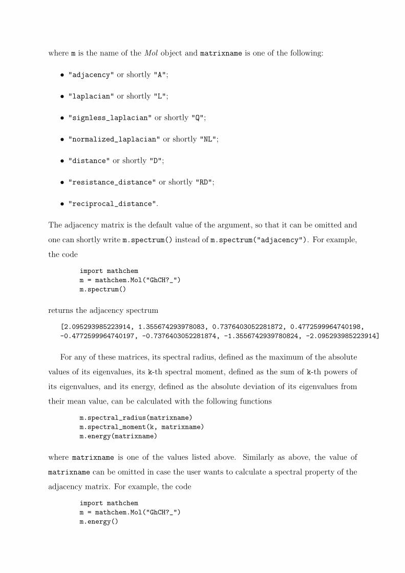
The adjacency matrix is the default value of the argument, so that it can be omitted and

one can shortly write m.spectrum() instead of m.spectrum("adjacency"). For example,

the code

import mathchem

m = mathchem.Mol("GhCH?_")

m.spectrum()

returns the adjacency spectrum

[2.095293985223914, 1.355674293978083, 0.7376403052281872, 0.4772599964740198,

-0.4772599964740197, -0.7376403052281874, -1.3556742939780824, -2.095293985223914]

For any of these matrices, its spectral radius, defined as the maximum of the absolute

values of its eigenvalues, its k-th spectral moment, defined as the sum of k-th powers of

its eigenvalues, and its energy, defined as the absolute deviation of its eigenvalues from

their mean value, can be calculated with the following functions

m.spectral_radius(matrixname)

m.spectral_moment(k, matrixname)

m.energy(matrixname)

where matrixname is one of the values listed above. Similarly as above, the value of

matrixname can be omitted in case the user wants to calculate a spectral property of the

adjacency matrix. For example, the code

import mathchem

m = mathchem.Mol("GhCH?_")

m.energy()

returns the (usual) graph energy

9.3317371618084071

The incidence matrix is not a square matrix in general, so that the incidence energy

is defined as the sum of its singular values. It is calculated with the function

m.incidence_energy()

MathChem also contains the corresponding functions for calculating spectral proper-

ties of an arbitrary user-supplied matrix matrix, represented as a two-dimensional array:

mathchem.spectrum(matrix)

mathchem.spectral_radius(matrix)

mathchem.spectral_moment(k, matrix)

mathchem.energy(matrix)

For example, the code

matrix = [[1,0,1],[0,1,0],[0,1,1]]

mathchem.spectrum(matrix)

returns

[2.0, 1.0, 0.0]

We should add here that, for performance reasons, MathChem calculates invariants

of a Mol object on demand and then saves the results for future use. Every Mol object

has its own set of private variables which is used as a cache for this purpose. This way,

MathChem avoids unnecessary recalculation of resource consuming data, such as matrices

or their spectral properties. For example, suppose that we want to calculate two distance-

based invariants, the diameter and the distance energy of a molecular graph:

import mathchem

m = mathchem.Mol("GhCH?_")

print m.diameter(), m.energy("distance")

Both of these functions need a distance matrix of the molecular graph, which is calcu-

lated internally during the first function call m.diameter() and then reused, without

recalculation, in the second function call m.energy("distance").

Table 5: Topological indices

Topological index Class method

The first Zagreb Index zagreb_m1_index()

The second Zagreb Index zagreb_m2_index()

Connectivity index (R(power)) connectivity_index(power)

Randic Index (R(-1/2)) randic_index()

Sum-Connectivity index sum_connectivity_index()

Geometric-Arithmetic index geometric_arithmetic_index()

Eccentric Connectivity Index eccentric_connectivity_index()

Atom-Bond Connectivity Index (ABC) atom_bond_connectivity_index()

Estrada Index (EE) of a graph matrix estrada_index(matrixname)

Degree Distance (DD) degree_distance()

Reverse Degree Distance (rDD) reverse_degree_distance()

Molecular Topological Index (MTI) molecular_topological_index()

Eccentric Distance Sum eccentric_distance_sum()

Balaban J index balaban_j_index()

Sum-Balaban index sum_balaban_index()

Kirchhoff Index (Kf) kirchhoff_index()

Wiener Index (W) wiener_index()

Terminal Wiener Index (TW) terminal_wiener_index()

Reverse Wiener Index (RW) reverse_wiener_index()

Hyper-Wiener Index (WW) hyper_wiener_index()

Harary Index (H) harary_index()

Laplacian-like energy (LEL) LEL()

The first Zagreb coindex zagreb_m1_coindex()

The second Zagreb coindex zagreb_m2_coindex()

log(Multiplicative Sum Zagreb index) multiplicative_sum_zagreb_index()

log(Multiplicative P1 Zagreb index) multiplicative_p1_zagreb_index()

log(Multiplicative P2 Zagreb index) multiplicative_p2_zagreb_index()

5.3 Topological indices

MathChem package implements most popular topological indices. The full list of imple-

mented indices is given in Tables 5 and 6. If necessary, see [1] for definitions and further

references.

For example, the following code

import mathchem

m = mathchem.Mol("GhCH?_")

print m.zagreb_m1_index(), m.zagreb_m2_index()

returns

30 31

In addition, MathChem implements all 148 discrete Adriatic indices, recently intro-

duced by Vukicevic and Gasperov [29] (see also [30]). The general definition of a discrete

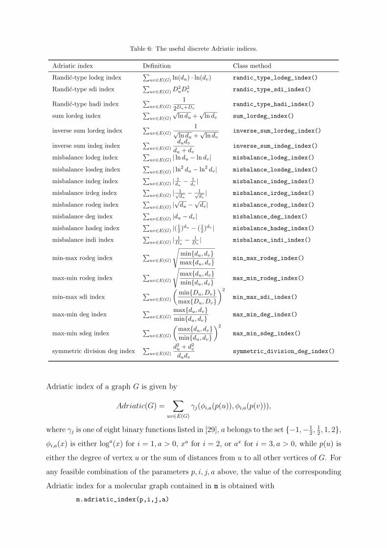
Table 6: The useful discrete Adriatic indices.

Adriatic index Definition Class method

Randic-type lodeg index∑

uv∈E(G) ln(du) · ln(dv) randic_type_lodeg_index()

Randic-type sdi index∑

uv∈E(G) D2uD

2v randic_type_sdi_index()

Randic-type hadi index∑

uv∈E(G)

1

2Du+Dvrandic_type_hadi_index()

sum lordeg index∑

uv∈E(G)

√ln du +

√ln dv sum_lordeg_index()

inverse sum lordeg index∑

uv∈E(G)

1√ln du +

√ln dv

inverse_sum_lordeg_index()

inverse sum indeg index∑

uv∈E(G)

dudvdu + dv

inverse_sum_indeg_index()

misbalance lodeg index∑

uv∈E(G) | ln du − ln dv| misbalance_lodeg_index()

misbalance losdeg index∑

uv∈E(G) | ln2 du − ln2 dv| misbalance_losdeg_index()

misbalance indeg index∑

uv∈E(G) |1du− 1

dv| misbalance_indeg_index()

misbalance irdeg index∑

uv∈E(G) |1√du− 1√

dv| misbalance_irdeg_index()

misbalance rodeg index∑

uv∈E(G) |√du −

√dv| misbalance_rodeg_index()

misbalance deg index∑

uv∈E(G) |du − dv| misbalance_deg_index()

misbalance hadeg index∑

uv∈E(G) |(12 )du − ( 1

2 )dv | misbalance_hadeg_index()

misbalance indi index∑

uv∈E(G) |1

Du− 1

Dv| misbalance_indi_index()

min-max rodeg index∑

uv∈E(G)

√min{du, dv}max{du, dv}

min_max_rodeg_index()

max-min rodeg index∑

uv∈E(G)

√max{du, dv}min{du, dv}

max_min_rodeg_index()

min-max sdi index∑

uv∈E(G)

(min{Du, Dv}max{Du, Dv}

)2

min_max_sdi_index()

max-min deg index∑

uv∈E(G)

max{du, dv}min{du, dv}

max_min_deg_index()

max-min sdeg index∑

uv∈E(G)

(max{du, dv}min{du, dv}

)2

max_min_sdeg_index()

symmetric division deg index∑

uv∈E(G)

d2u + d2vdudv

symmetric_division_deg_index()

Adriatic index of a graph G is given by

Adriatic(G) =∑

uv∈E(G)

γj(φi,a(p(u)), φi,a(p(v))),

where γj is one of eight binary functions listed in [29], a belongs to the set {−1,−12, 12, 1, 2},

φi,a(x) is either loga(x) for i = 1, a > 0, xa for i = 2, or ax for i = 3, a > 0, while p(u) is

either the degree of vertex u or the sum of distances from u to all other vertices of G. For

any feasible combination of the parameters p, i, j, a above, the value of the corresponding

Adriatic index for a molecular graph contained in m is obtained with

m.adriatic_index(p,i,j,a)

The list of all feasible combinations of the parameters p, i, j, a is obtained with

mathchem.all_adriatic()

Vukicevic and Gasperov [29] also introduced naming convention for Adriatic indices,

that is fully implemented in MathChem. Instead of m.adriatic_index(0, 2, 7, 0.5),

for example, one can equivalenty use m.max_min_rodeg_index(). The name of the Adri-

atic index for a given parameter set can be obtained with

mathchem.adriatic_name(p,i,j,a)

Table 6 lists the names of twenty discrete Adriatic indices that are identified as useful for

QSAR/QSPR studies in [29].

The use of these functions may be illustrated with the following code:

import mathchem

m = mathchem.Mol("GhCH?_")

for x in mathchem.all_adriatic():

print mathchem.adriatic_name(*x), m.adriatic_index(*x)

Here, mathchem.all_adriatic() returns the list of all feasible parameter sets (repre-

sented as fourtuples), and the for command iterates x through this list. The construc-

tion *x “opens up” each fourtuple into four separate arguments, which are then used as

arguments to MathChem functions. The result are the names and the values of all 148

discrete Adriatic indices calculated for the molecular graph in m:

Randic type lordeg 2.84389164788

Randic type lodeg 2.72994898165

Randic type losdeg 2.61649032574

sum lordeg 9.61910088844

sum lodeg 9.36426245425

...

6 More elaborate examples of MathChem use

We give here a few more elaborate examples of MathChem use, which illustrate both the

power and the simplicity of the package, as well as the possibilities offered by joint use of

MathChem with NetworkX or Sage.

6.1 Examples of integration with NetworkX and Sage

NetworkX [17] is a popular Python package aimed for creation, manipulation, and study of

the structure, dynamics, and functions of complex networks. Sage [16] is a powerful open-

source mathematics software system, aimed as a free alternative to commercial systems

like Mathematica or MATLAB, which has an interactive web-based user interface and

contains more than 100 mathematical packages, including NetworkX.

MathChem contains two functions which translate the molecular graph contained in

a Mol object m into the graph formats used by Sage (g) and NetworkX (h), respectively:

g = m.sage_graph()

h = m.NX_graph()

On the other hand, if a graph g is provided in Sage format, the corresponding Mol object

m may be constructed by using the function graph6_string() from Sage’s Graph class:

m = mathchem.Mol(g.graph6_string())

Next, if a graph h is provided in NetworkX format, the corresponding Mol object m may

be constructed by using the function edges() from NetworkX:

m = mathchem.Mol()

m.read_edgelist(h.edges())

For example, to list all independent sets of a molecular graph, one can use functions

find_cliques and complement from NetworkX:

import mathchem

import networkx

m = mathchem.Mol("GhCH?_")

g = m.NX_graph()

list(networkx.find_cliques(networkx.complement(g)))

which returns

[[0, 4, 7, 2],

[0, 4, 7, 6],

[0, 5, 2, 7],

[0, 5, 6, 3],

[0, 5, 6, 7],

[1, 6, 4, 7],

[1, 6, 5, 3],

[1, 6, 5, 7]]

In the next example, to find the matching polynomial of a molecular graph, one can

use function matching_polynomial from Sage:

import mathchem

m = mathchem.Mol("GhCH?_")

g = m.sage_graph()

g.matching_polynomial()

which returns

x^8 - 7*x^6 + 13*x^4 - 7*x^2 + 1

Sage can also be used for visualization of molecular graphs:

import mathchem

m = mathchem.Mol("GhCH?_")

g = m.sage_graph()

g.show()

Resulting drawing is shown in Fig. 1.

Figure 1: Molecular graph can be visualized with show() method from Sage.

MathChem can also be used to calculate topological indices for graphs created in Sage.

The following example calculates Randic index of a random tree with 10 vertices:

import mathchem

g = graphs.RandomTree(10)

m = mathchem.Mol(g.graph6_string())

m.randic_index()

6.2 Correlation examples

We now give examples of creating bar charts, scatter plots and histograms for a list of

molecular graphs. For this purpose, we use MathChem from within Sage (see Subsection

2.2 for installing MathChem as a Sage module). As a test bed, we use compounds from

the NCI online database with NSC number from 1 to 5000.

Start Sage and import MathChem:

sage: import mathchem

To import all compounds with NSC number from 1 to 5000 in the NCI online database

to the list mols, use:

sage: mols = mathchem.read_from_NCI_by_NSC("1-5000")

sage: len(mols)

4935

The actual number of retrieved records is 4935, because the NCI database has gaps in

NSC numbers. The following code filters the list mols for connected molecular graphs:

sage: mols_c = filter(lambda m: m.is_connected(), mols)

sage: len(mols_c)

4800

Python’s filter function iterates through every item of the list mols, checks whether it

is a connected graph and if so appends the item to the new list mols_c. In the code above

we also used Python’s lambda-construct lambda m: m.is_connected() which allows to

create small functions on the fly and make code shorter.

Now we calculate Randic index for every item of the list mols_c and put calculated

values into a new list ri:

sage: ri = [m.randic_index() for m in mols_c]

The minimum and maximum entries of the list are obtained with functions min and max:

sage: print min(ri), max(ri)

1.0 42.1016302944

The bar chart of values in the list ri can be obtained with Sage’s function bar_chart:

sage: bar_chart(ri)

Resulting bar chart is shown in Fig. 2.

Figure 2: Bar chart of Randic index for connected NCI compounds with NSC numbers from 1 to 5000.

We can now explore correlation of Randic index with Harary index for these com-

pounds. Let us calculate the Harary index as well:

sage: hi = [m.harary_index() for m in mols_c]

To get the scatter plot of values from the lists ri and hi, we use Sage’s scatter_plot

function. This function takes the list of pairs of values as its single argument. We can

use Python’s zip function to make such list of pairs out of two given lists:

sage: scatter_plot(zip(ri,hi))

Resulting scatter plot is shown in Fig. 3.

Figure 3: Scatter plot of Randic index versus the Harary index for connected NCI compounds with NSCnumbers from 1 to 5000.

To get the histogram showing the distribution of orders of molecular graphs contained

in the list mols_c, we first create the list containing the order of these graphs:

sage: orders = [m.order() for m in mols_c]

Then we create a new list that will contain number of molecular graphs for each different

order. This list has to have one more element than the maximum order (as the list

elements are indexed from 0) and the list elements are initially set to zeros:

sage: hist_data = [0]*(max(orders)+1)

We now iterate through the list of orders and count appearances of each order:

sage: for i in orders: hist_data[i] += 1

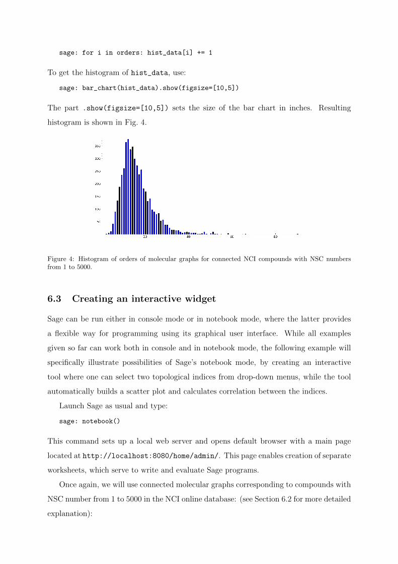
To get the histogram of hist_data, use:

sage: bar_chart(hist_data).show(figsize=[10,5])

The part .show(figsize=[10,5]) sets the size of the bar chart in inches. Resulting

histogram is shown in Fig. 4.

Figure 4: Histogram of orders of molecular graphs for connected NCI compounds with NSC numbersfrom 1 to 5000.

6.3 Creating an interactive widget

Sage can be run either in console mode or in notebook mode, where the latter provides

a flexible way for programming using its graphical user interface. While all examples

given so far can work both in console and in notebook mode, the following example will

specifically illustrate possibilities of Sage’s notebook mode, by creating an interactive

tool where one can select two topological indices from drop-down menus, while the tool

automatically builds a scatter plot and calculates correlation between the indices.

Launch Sage as usual and type:

sage: notebook()

This command sets up a local web server and opens default browser with a main page

located at http://localhost:8080/home/admin/. This page enables creation of separate

worksheets, which serve to write and evaluate Sage programs.

Once again, we will use connected molecular graphs corresponding to compounds with

NSC number from 1 to 5000 in the NCI online database: (see Section 6.2 for more detailed

explanation):

sage: import mathchem

sage: mols = mathchem.read_from_NCI_by_NSC("1-5000")

sage: mols_c = filter(lambda m: m.is_connected(), mols)

The next command defines a list of topological indices to appear in drop-down menus:

sage: methods = ["order", "diameter", "energy", "incidence_energy", "randic_index",

"zagreb_m1_index", "zagreb_m2_index", "eccentric_connectivity_index",

"atom_bond_connectivity_index", "estrada_index", "eccentric_distance_sum",

"reverse_degree_distance", "molecular_topological_index", "degree_distance",

"balaban_j_index", "kirchhoff_index", "wiener_index", "harary_index", "LEL",

"reverse_wiener_index", "hyper_wiener_index", "terminal_wiener_index",

"randic_type_lodeg_index", "randic_type_sdi_index", "randic_type_hadi_index"]

Next we include ScyPy statistical library in order to use its linear regression methods:

sage: import scipy.stats as stats

We are now ready to write an interactive tool:

@interact

def index_correlations(index_A = selector(methods,label="Index A"), \

index_B = selector(methods,label="Index B")):

data_A = [getattr(m, index_A)() for m in mols_c]

data_B = [getattr(m, index_B)() for m in mols_c]

data = zip(data_A, data_B)

slope, intercept, r, ttprob, stderr = stats.linregress(data)

print "Correlation coefficient: ", r

canvas = scatter_plot(data) + plot(slope*x+intercept,min(data_A),max(data_A))

canvas.show(figsize=[10,4], axes_labels=[index_A, index_B])

The function above is called automatically whenever its arguments are changing their

values. Its arguments index_A and index_B are defined as visual selectors of all methods

appearing in methods. Python construct getattr(m, index_A)() calls a method whose

name is contained in index_A of the Mol object m. This is used in for loop, which

then results in the values of selected topological index to be put in the list data_A,

respectively data_B. The two list are then “zipped” to produce a list of pairs, after which

linear regression is applied, with the results—scatter plot and the best fit line—visually

presented in canvas. The look of the resulting tool is presented in Fig. 5.

7 Conclusion

We have described MathChem, a Python package for calculating topological indices, and

provided examples of its joint use with other well known open-source products such as Sage

Figure 5: Interactive widget.

or NetworkX. MathChem package does not solve problems out-of-the-box, but instead it

provides a flexible and easily expandable framework for computational research in mathe-

matical chemistry. All contributions or requests for implementation are welcome through

MathChem’s Github homepage: https://github.com/hamster3d/Mathchem-package

or by sending e-mail to authors.

Acknowledgement. The research work of the authors was supported by Research Program

No. P1-0285 and Research Project No. J1-4021 of the Slovenian Research Agency, and

Research Grant No. ON174033 of the Ministry of Education and Science of Serbia.

References

[1] R. Todeschini, V. Consonni, Handbook of Molecular Descriptors, Wiley–VCH, Weinheim,2000.

[2] A. Mauri, V. Consonni, M. Pavan, R. Todeschini, Dragon software: an easy approach tomolecular descriptors calculation, MATCH Commun. Math. Comput. Chem. 56 (2006),237–248.

[3] Talete, Dragon 6, http://www.talete.mi.it/products/dragon description.htm, accessed Nov5, 2013.

[4] A. Kerber, R. Laue, M. Meringer, C. Rucker, MOLGEN-QSPR, a Software Package forthe Study of Quantitative Structure Property Relationships, MATCH Commun. Math.Comput. Chem. 51 (2004), 187–204.

[5] J. Braun, M. Meringer, C. Rucker, Molecular Structure Generation,http://molgen.de/?src=documents/molgenqspr.html, accessed Nov 5, 2013.

[6] ChemAxon, GenerateMD, http://www.chemaxon.com/jchem/doc/user/GenerateMD.html,accessed Sep 5, 2013.

[7] J. Liu, J. Feng, A. Brooks, S. Young, PowerMV: A software environment for statisti-cal analysis, molecular viewing, descriptor generation, and similarity search, available athttp://nisla05.niss.org/PowerMV/?q=PowerMV/, accessed Sep 5, 2013.

[8] EduSoft, Molconn-Z, http://www.edusoft-lc.com/molconn/, accessed Sep 5, 2013.

[9] Semichem, CODESSA, available at http://www.semichem.com/codessa/, accessed Sep 5,2013.

[10] V.J. Sykora, Chemical Descriptors Library (CDL), available at http://sourceforge.net/projects/cdelib/, accessed Sep 5, 2013.

[11] J.C Stalring, L.A. Carlsson, P. Almeida, S. Boyer, AZOrange—High performance opensource machine learning for QSAR modeling in a graphical programming environment, J.Cheminform. 3 (2011), 28.

[12] C.W. Yap, PaDEL-Descriptor: An open source software to calculate molecular descriptorsand fingerprints, J. Comput. Chem. 32 (2011), 1466–1474

[13] National University of Singapore, PaDEL-Descriptor, http://padel.nus.edu.sg/software/padeldescriptor/index.html, accessed Nov 5, 2013.

[14] C. Steinbeck, Y. Han, S. Kuhn, O. Horlacher, E. Luttmann, E.L. Willighagen, The Chem-istry Development Kit (CDK): An Open-Source Java Library for Chemo- and Bioinformat-ics, J. Chem. Inf. Comput. Sci. 43 (2003) 493–500.

[15] Python Software Foundation, Python Programming Language—Oficial Website,http://www.python.org/, accessed Sep 6, 2013.

[16] W. Stein, Sage: Open Source Mathematics Software, http://www.sagemath.org/, accessedSep 6, 2013.

[17] NetworkX developer team, High-productivity software for complex networks,http://networkx.github.io/, accessed Sep 6, 2013.

[18] A.A. Hagberg, D.A. Schult, P.J. Swart, Exploring network structure, dynamics, and func-tion using NetworkX, in: Proceedings of the 7th Python in Science Conference SciPy2008(G. Varoquaux, T. Vaught, J. Millman, eds.), Pasadena, 2008, pp. 11–15.

[19] SciPy developers, SciPy, http://www.scipy.org/, accessed Sep 6, 2013.

[20] NumPy developer team, NumPy, http://www.numpy.org/, accessed Sep 6, 2013.

[21] N.M O’Boyle, M. Banck, C.A. James, C. Morley, T. Vandermeersch, G.R. Hutchison, OpenBabel: An open chemical toolbox, J. Cheminf. 3 (2011), 33.

[22] Open Babel: The Open Source Chemistry Toolbox, http://openbabel.org/wiki/Main Page,accessed Nov 5, 2013.

[23] NCI/CADD Group and Xemistry GmbH, Enhanced NCI Database Browser 2.2,http://cactus.nci.nih.gov/ncidb2.2/, accessed Sep 29, 2013.

[24] B.D. McKay, graph6 and sparse6 graph formats, http://cs.anu.edu.au/˜bdm/data/formats.html, accessed Sep 29, 2013.

[25] B.D. McKay, Graphs, http://cs.anu.edu.au/˜bdm/data/graphs.html, accessed Sep 29,2013.

[26] G. Royle, Combinatorial Catalogues, http://school.maths.uwa.edu.au/˜gordon/data.html,accessed Sep 29, 2013.

[27] B.D. McKay, A. Piperno, nauty and Traces, http://pallini.di.uniroma1.it/, accessed Sep29, 2013.

[28] B.D. McKay, G. Brinkmann, plantri and fullgen, http://cs.anu.edu.au/˜bdm/plantri/, ac-cessed Sep 29, 2013.

[29] D. Vukicevic, M. Gasperov, Bond Additive Modelling 1. Adriatic Indices, Croat. Chem.Acta 83 (2010), 243–260.

[30] D. Vukicevic, Bond Additive Modeling 2. Mathematical Properties of Max-Min RodegIndex, Croat. Chem. Acta 83 (2010), 261–273.