MATH 5520 Numerical Integration 1. - Home › Department...
21
MATH 5520 Numerical Integration 1. Dmitriy Leykekhman Spring 2009 D. Leykekhman - MATH 5520 Finite Element Methods 1 Numerical Integration 1 – 1
Transcript of MATH 5520 Numerical Integration 1. - Home › Department...

MATH 5520Numerical Integration 1.
Dmitriy Leykekhman
Spring 2009
D. Leykekhman - MATH 5520 Finite Element Methods 1 Numerical Integration 1 – 1
Numerical Integration.
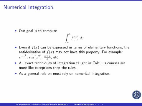
I Our goal is to compute ∫ b
a
f(x) dx.
I Even if f(x) can be expressed in terms of elementary functions, theantiderivative of f(x) may not have this property. For example:
e−x2, sin (x2), sin x
x , etc.
I All exact techniques of integration taught in Calculus courses aremore like exceptions then the rules.
I As a general rule on must rely on numerical integration.
D. Leykekhman - MATH 5520 Finite Element Methods 1 Numerical Integration 1 – 2

Numerical Integration.
I We want to approximate the integral of a function f by a weightedsum of function values:∫ b
a
f(x) dx ≈n∑i=0
wif(xi).
I In the above formula xi ∈ [a, b] are called the nodes of theintegration formula and wi are called the weights of the integrationformula.
I When we approximate∫ baf(x) dx by
∑ni=0 wif(xi) we speak of
numerical integration or numerical quadrature
I∑ni=0 wif(xi) is called a quadrature formula.
D. Leykekhman - MATH 5520 Finite Element Methods 1 Numerical Integration 1 – 3
Numerical Integration.
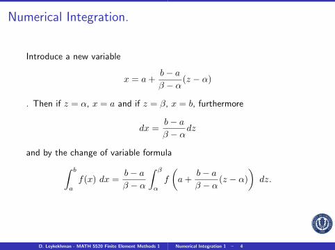
Introduce a new variable
x = a+b− aβ − α
(z − α)
. Then if z = α, x = a and if z = β, x = b, furthermore
dx =b− aβ − α
dz
and by the change of variable formula∫ b
a
f(x) dx =b− aβ − α
∫ β
α
f
(a+
b− aβ − α
(z − α))dz.
D. Leykekhman - MATH 5520 Finite Element Methods 1 Numerical Integration 1 – 4

Numerical Integration.
Thus, if we have computed weights wi and nodes zi for the numericalintegration on an interval [α, β], then we can use the above identity toapproximate the integral of f over any interval [a, b] (assuming, of course,that this integral exist) by∫ b
a
f(x) dx =b− aβ − α
∫ β
α
f
(a+
b− aβ − α
(z − α))dz
≈ b− aβ − α
n∑i=0
wif
(a+
b− aβ − α
(zi − α)).
D. Leykekhman - MATH 5520 Finite Element Methods 1 Numerical Integration 1 – 5

Numerical Integration.
That is, the weights wi and nodes xi for the numerical integration on theinterval [a, b] are
wi =b− aβ − α
wi, xi = a+b− aβ − α
(zi − α).
This means it is sufficient to compute weights and nodes for thenumerical integration on a certain interval like [0, 1] or [−1, 1], oftencalled the reference intervals.
D. Leykekhman - MATH 5520 Finite Element Methods 1 Numerical Integration 1 – 6
Numerical Integration.
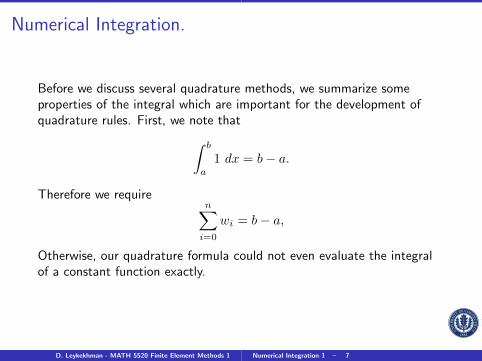
Before we discuss several quadrature methods, we summarize someproperties of the integral which are important for the development ofquadrature rules. First, we note that∫ b
a
1 dx = b− a.
Therefore we requiren∑i=0
wi = b− a,
Otherwise, our quadrature formula could not even evaluate the integralof a constant function exactly.
D. Leykekhman - MATH 5520 Finite Element Methods 1 Numerical Integration 1 – 7

Numerical Integration.
Another property of the integral is
f(x) ≥ 0 =⇒∫ b
a
f(x) dx ≥ 0.
Ifwi ≥ 0, i = 0, . . . , n,
thenn∑i=0
wif(xi) ≥ 0,
for all functions f(x) ≥ 0.
D. Leykekhman - MATH 5520 Finite Element Methods 1 Numerical Integration 1 – 8

Numerical Integration.
I We also desire our numerical quadrature to be efficient.
I Efficiency often depends upon the number of function evaluations.
I Typically to evaluate f at xi is more expensive than form a linearcombination of function values.
D. Leykekhman - MATH 5520 Finite Element Methods 1 Numerical Integration 1 – 9

Interpolatory Quadrature Formulas.
Basic idea: if p(x) is some function such that
p(x) ≈ f(x),
then ∫ b
a
p(x) dx ≈∫ b
a
f(x) dx
Thus we need a function p(x) which close to f(x) and easy to integrate.
D. Leykekhman - MATH 5520 Finite Element Methods 1 Numerical Integration 1 – 10

Interpolatory Quadrature Formulas.
Chose nodes x0, x1, . . . , xn in the interval [a, b] and compute thepolynomial P (f |x0, . . . , xn) of degree less or equal to n interpolating fat x0, x1, . . . , xn. If we use the approximation
f(x) ≈ P (f |x0, . . . , xn)(x),
then we obtain an approximation for the integral:∫ b
a
f(x) dx ≈∫ b
a
P (f |x0, . . . , xn)(x) dx (1). (1)
These types of quadrature formulas are called interpolatory quadratureformulas.
D. Leykekhman - MATH 5520 Finite Element Methods 1 Numerical Integration 1 – 11

Interpolatory Quadrature Formulas.
It is useful to represent the interpolation polynomial using the Lagrangebasis,
P (f |x0, . . . , xn)(x) =n∑i=0
f(xi)n∏j=0j 6=i
x− xjxi − xj
.
If we substitute this representation of the interpolation polynomial into(1), then we obtain∫ b
a
f(x) dx ≈∫ b
a
P (f |x0, . . . , xn)(x) dx
=∫ b
a
n∑i=0
f(xi)n∏j=0j 6=i
x− xjxi − xj
dx
=n∑i=0
f(xi)∫ b
a
n∏j=0j 6=i
x− xjxi − xj
dx.
D. Leykekhman - MATH 5520 Finite Element Methods 1 Numerical Integration 1 – 12
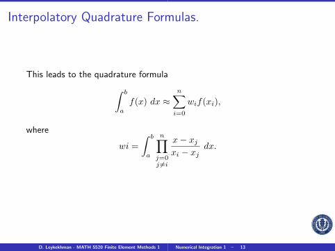
Interpolatory Quadrature Formulas.
This leads to the quadrature formula∫ b
a
f(x) dx ≈n∑i=0
wif(xi),
where
wi =∫ b
a
n∏j=0j 6=i
x− xjxi − xj
dx.
D. Leykekhman - MATH 5520 Finite Element Methods 1 Numerical Integration 1 – 13
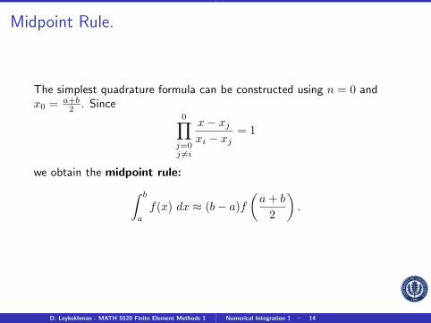
Midpoint Rule.
The simplest quadrature formula can be constructed using n = 0 andx0 = a+b
2 . Since0∏j=0j 6=i
x− xjxi − xj
= 1
we obtain the midpoint rule:∫ b
a
f(x) dx ≈ (b− a)f(a+ b
2
).
D. Leykekhman - MATH 5520 Finite Element Methods 1 Numerical Integration 1 – 14
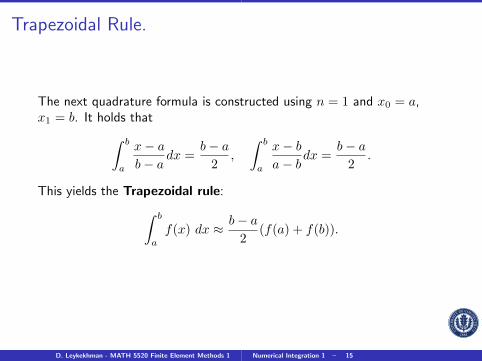
Trapezoidal Rule.
The next quadrature formula is constructed using n = 1 and x0 = a,x1 = b. It holds that∫ b
a
x− ab− a
dx =b− a
2,
∫ b
a
x− ba− b
dx =b− a
2.
This yields the Trapezoidal rule:∫ b
a
f(x) dx ≈ b− a2
(f(a) + f(b)).
D. Leykekhman - MATH 5520 Finite Element Methods 1 Numerical Integration 1 – 15

Simpson rule.
The next quadrature formula is constructed using n = 2 and x0 = a,x1 = b+a
2 , x2 = b. Then∫ b
a
x− b+a2
a− b+a2
x− ba− b
dx =b− a
6,∫ b
a
x− ab+a2 − a
x− bb+a2 − b
dx = 4b− a
6,∫ b
a
x− b+a2
b− b+a2
x− bb− a
dx =b− a
6.
This yields the Simpson rule:∫ b
a
f(x) dx ≈ b− a6
(f(a) + 4f
(b+ a
2)
+ f(b)).
D. Leykekhman - MATH 5520 Finite Element Methods 1 Numerical Integration 1 – 16

Newton Cotes Quadrature Formula.
If we have equidistant points
xi = a+ ih, i = 0, . . . , n, h =b− an
,
then the resulting interpolatory quadrature formula is called a closedNewton Cotes quadrature formula (a and b are nodes). In this casewe can use the substitution x = a+ sh, to compute
wi =∫ b
a
n∏j=0j 6=i
x− xjxi − xj
dx = (b− a) 1n
∫ n
0
n∏j=0j 6=i
s− ji− j
ds.
D. Leykekhman - MATH 5520 Finite Element Methods 1 Numerical Integration 1 – 17
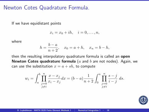
Newton Cotes Quadrature Formula.
If we have equidistant points
xi = x0 + ih, i = 0, . . . , n,
where
h =b− an+ 2
, x0 = a+ h, xn = b− h,
then the resulting interpolatory quadrature formula is called an openNewton Cotes quadrature formula (a and b are not nodes). Again, wecan use the substitution x = a+ sh, to compute
wi =∫ b
a
n∏j=0j 6=i
x− xjxi − xj
dx = (b− a) 1n+ 2
∫ n
0
n∏j=0j 6=i
s− ji− j
ds.
D. Leykekhman - MATH 5520 Finite Element Methods 1 Numerical Integration 1 – 18
Newton Cotes Quadrature Formula.
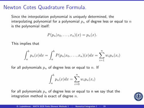
Since the interpolation polynomial is uniquely determined, theinterpolating polynomial for a polynomial pn of degree less or equal to nis the polynomial itself:
P (pn|x0, . . . , xn)(x) = pn(x).
This implies that∫ b
a
pn(x)dx =∫ b
a
P (pn|x0, . . . , xn)(x)dx =n∑i=1
wipn(xi)
for all polynomials pn of degree less or equal to n. If∫ b
a
pn(x)dx =n∑i=0
wipn(xi)
for all polynomials pn of degree less or equal to n we say that theintegration method is exact of degree n.
D. Leykekhman - MATH 5520 Finite Element Methods 1 Numerical Integration 1 – 19
Newton Cotes Quadrature Formula.
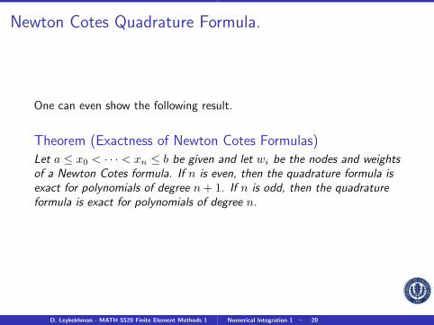
One can even show the following result.
Theorem (Exactness of Newton Cotes Formulas)Let a ≤ x0 < · · · < xn ≤ b be given and let wi be the nodes and weightsof a Newton Cotes formula. If n is even, then the quadrature formula isexact for polynomials of degree n+ 1. If n is odd, then the quadratureformula is exact for polynomials of degree n.
D. Leykekhman - MATH 5520 Finite Element Methods 1 Numerical Integration 1 – 20
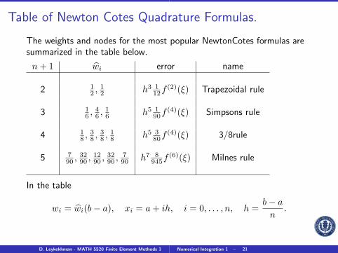
Table of Newton Cotes Quadrature Formulas.
The weights and nodes for the most popular NewtonCotes formulas aresummarized in the table below.
n+ 1 wi error name
2 12 ,
12 h3 1
12f(2)(ξ) Trapezoidal rule
3 16 ,
46 ,
16 h5 1
90f(4)(ξ) Simpsons rule
4 18 ,
38 ,
38 ,
18 h5 3
80f(4)(ξ) 3/8rule
5 790 ,
3290 ,
1290 ,
3290 ,
790 h7 8
945f(6)(ξ) Milnes rule
In the table
wi = wi(b− a), xi = a+ ih, i = 0, . . . , n, h =b− an
.
D. Leykekhman - MATH 5520 Finite Element Methods 1 Numerical Integration 1 – 21