MATH 3795 Lecture 4. Solving Linear Systems 2
35
MATH 3795 Lecture 4. Solving Linear Systems 2 Dmitriy Leykekhman Fall 2008 Goals I Understand what happens when you type [L, U, P ]= lu(A). I Understand how to use matrix decompositions. I Computational aspects. D. Leykekhman - MATH 3795 Introduction to Computational Mathematics Floating Point Arithmetic – 1
Transcript of MATH 3795 Lecture 4. Solving Linear Systems 2

MATH 3795Lecture 4. Solving Linear Systems 2
Dmitriy Leykekhman
Fall 2008
GoalsI Understand what happens when you type [L, U, P ] = lu(A).
I Understand how to use matrix decompositions.
I Computational aspects.
D. Leykekhman - MATH 3795 Introduction to Computational Mathematics Floating Point Arithmetic – 1

Motivation for LU DecompositionI The present form of the Gaussian elimination with partial pivoting is
useful to solve a linear system Ax = b.
I However, we need it to be more versatile. For example, suppose wehave used Gaussian elimination with partial pivoting to solve Ax = b(cost ≈ 2n3/3 flops , where n is the size of the system). If we aregiven another right hand side c and are asked to solve Ax = c,currently we have to redo all computations and solve the new linearsystem at a cost of ≈ 2n3/3 flops , even through most of theoperations are identical to the ones we have executed before. (Thissituation arises, for example, in the numerical solution of timedependent differential equations.)
I The LU-decomposition removes these shortcomings.
I We will first reorganize the computations performed in the Gaussianelimination with partial pivoting and separate computationsperformed on A from those performed on the right hand side. Thenwe will interpret these operations mathematically to be able to reusethe computations to perform other tasks, for example to solve thelinear system AT y = c.
D. Leykekhman - MATH 3795 Introduction to Computational Mathematics Floating Point Arithmetic – 2
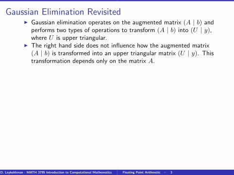
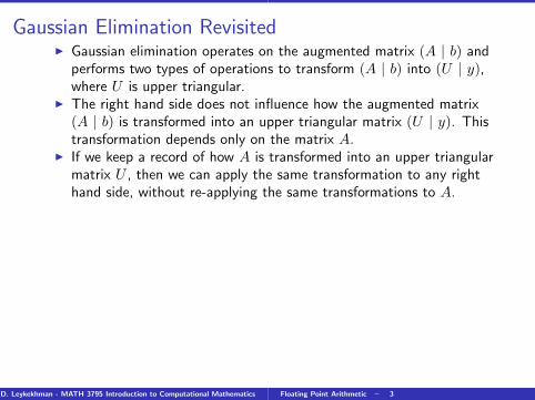
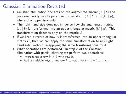
Gaussian Elimination RevisitedI Gaussian elimination operates on the augmented matrix (A | b) and
performs two types of operations to transform (A | b) into (U | y),where U is upper triangular.
I The right hand side does not influence how the augmented matrix(A | b) is transformed into an upper triangular matrix (U | y). Thistransformation depends only on the matrix A.
I If we keep a record of how A is transformed into an upper triangularmatrix U , then we can apply the same transformation to any righthand side, without re-applying the same transformations to A.
I What operations are performed? In step k of the Gaussianelimination with partial pivoting we perform two operations:
I Interchange a row i0 > k with row k.I Add a multiple −lik times row k to row i for i = k + 1, . . . , n.
I How do we record this?I Introduce an integer array ipivt. Set
ipivt(k) = i0
when the k-th step the rows k and i0 are interchanged.I Store the −lik in the (i, k)-th position of the array that originally
held A. (Remember that we add a multiple −lik times row k to rowi to eliminate the entry (i, k). Hence this storage can be reused.)
D. Leykekhman - MATH 3795 Introduction to Computational Mathematics Floating Point Arithmetic – 3

ExampleConsider the matrix 1 2 −1
2 1 0−1 2 2
After step k = 1 the vector ipivt and the matrix A are given by
ipivt = (2, , )
1 2 -1− 1
232 -1
12
52 2
After step k = 2 the vector ipivt and the matrix A are given by
ipivt = (2, 3, )
1 2 −1− 1
252 2
12 − 3
5 − 115
D. Leykekhman - MATH 3795 Introduction to Computational Mathematics Floating Point Arithmetic – 4

ExampleIf we want to solve the linear system Ax = b with
b =
021
We have to apply the same transformation to b
021
step 1−→
2−1
2
step 2−→
22
−11/5
and then solve 1 2 −1
0 52 2
0 0 − 115
x1
x2
x3
=
22
−11/5
by back substitution to obtain x1 = 1, x2 = 0, x3 = 1.
D. Leykekhman - MATH 3795 Introduction to Computational Mathematics Floating Point Arithmetic – 5

ExampleIf we want to solve the linear system Ax = b with
b =
021
We have to apply the same transformation to b 0
21
step 1−→
2−1
2
step 2−→
22
−11/5
and then solve 1 2 −10 5
2 20 0 − 11
5
x1
x2
x3
=
22
−11/5
by back substitution to obtain x1 = 1, x2 = 0, x3 = 1.
D. Leykekhman - MATH 3795 Introduction to Computational Mathematics Floating Point Arithmetic – 5

ExampleIf we want to solve the linear system Ax = b with
b =
021
We have to apply the same transformation to b 0
21
step 1−→
2−1
2
step 2−→
22
−11/5
and then solve 1 2 −1
0 52 2
0 0 − 115
x1
x2
x3
=
22
−11/5
by back substitution to obtain x1 = 1, x2 = 0, x3 = 1.
D. Leykekhman - MATH 3795 Introduction to Computational Mathematics Floating Point Arithmetic – 5

a11 a12 a13 · · · · · · a1,n−1 a1n
a21 a22 a23 · · · · · · a2,n−1 a2n
a31 a32 a33 · · · · · · a3,n−1 a3n
......
......
...an−1,1 an−1,2 an−1,3 · · · · · · an−1,n−1 an−1,n
an1 an2 an3 · · · · · · an,n−1 ann
↓
Step 1
↓
a11 a12 a13 · · · · · · a1,n−1 a1n
−l21 a22 a23 · · · · · · a2,n−1 a2n
−l31 a32 a33 · · · · · · a3,n−1 a3n
......
......
...−ln−1,1 an−1,2 an−1,3 · · · · · · an−1,n−1 an−1,n
−ln1 an2 an3 · · · · · · an,n−1 ann
↓
Step 2
↓D. Leykekhman - MATH 3795 Introduction to Computational Mathematics Floating Point Arithmetic – 6

Step 2
↓
a11 a12 a13 · · · · · · a1,n−1 a1n
−l21 a22 a23 · · · · · · a2,n−1 a2n
−l31 −l32 a33 · · · · · · a3,n−1 a3n
......
......
...−ln−1,1 −ln−1,2 an−1,3 · · · · · · an−1,n−1 an−1,n
−ln1 −ln2 an3 · · · · · · an,n−1 ann
↓
Step n-1
↓
a11 a12 a13 · · · · · · a1,n−1 a1n
−l21 a22 a23 · · · · · · a2,n−1 a2n
−l31 −l32 a33 · · · · · · a3,n−1 a3n
......
.... . .
......
......
.... . . an−1,n−1 an−1,n
−ln1 −ln2 −ln3 · · · · · · −ln,n−1 ann
D. Leykekhman - MATH 3795 Introduction to Computational Mathematics Floating Point Arithmetic – 7

Gaussian Elimination via Matrix Multiplications
Row interchange in step k can be expressed by multiplying with
Pk =
1. . .
10 1
1. . .
11 0
1. . .
1
← k
← ipivt(k)
from the left. Pk is a permutation matrix
D. Leykekhman - MATH 3795 Introduction to Computational Mathematics Floating Point Arithmetic – 8

Gaussian Elimination via Matrix Multiplications (cont)
Adding −li,k times row k to row i for i = k + 1, . . . , n is equivalent tomultiplying from the left with
Mk =
1. . .
1−lk+1,k
.... . .
−ln,k 1
Observe that matrix Mk is lower triangular and is called a Gausstransformation.
D. Leykekhman - MATH 3795 Introduction to Computational Mathematics Floating Point Arithmetic – 9

Gaussian Elimination via Matrix Multiplications (cont)
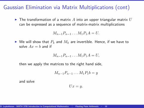
I The transformation of a matrix A into an upper triangular matrix Ucan be expressed as a sequence of matrix-matrix multiplications
Mn−1Pn−1 . . . M1P1A = U.
I We will show that Pk and Mk are invertible. Hence, if we have tosolve Ax = b and if
Mn−1Pn−1 . . . M1P1A = U,
then we apply the matrices to the right hand side,
Mn−1Pn−1 . . . M1P1b = y
and solveUx = y.
D. Leykekhman - MATH 3795 Introduction to Computational Mathematics Floating Point Arithmetic – 10
Gaussian Elimination via Matrix Multiplications (cont)
I The transformation of a matrix A into an upper triangular matrix Ucan be expressed as a sequence of matrix-matrix multiplications
Mn−1Pn−1 . . . M1P1A = U.
I We will show that Pk and Mk are invertible. Hence, if we have tosolve Ax = b and if
Mn−1Pn−1 . . . M1P1A = U,
then we apply the matrices to the right hand side,
Mn−1Pn−1 . . . M1P1b = y
and solveUx = y.
D. Leykekhman - MATH 3795 Introduction to Computational Mathematics Floating Point Arithmetic – 10
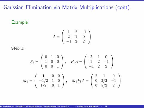
Gaussian Elimination via Matrix Multiplications (cont)
Example
A =
1 2 −12 1 0−1 2 2
Step 1:
P1 =
0 1 01 0 00 0 1
, P1A =
2 1 01 2 −1−1 2 2
M1 =
1 0 0−1/2 1 01/2 0 1
, M1P1A =
2 1 00 3/2 −10 5/2 2
D. Leykekhman - MATH 3795 Introduction to Computational Mathematics Floating Point Arithmetic – 11
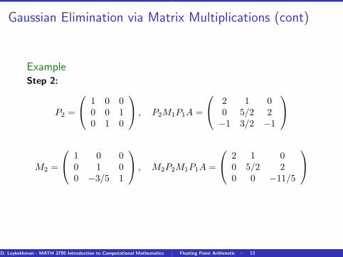
Gaussian Elimination via Matrix Multiplications (cont)
ExampleStep 2:
P2 =
1 0 00 0 10 1 0
, P2M1P1A =
2 1 00 5/2 2−1 3/2 −1
M2 =
1 0 00 1 00 −3/5 1
, M2P2M1P1A =
2 1 00 5/2 20 0 −11/5
D. Leykekhman - MATH 3795 Introduction to Computational Mathematics Floating Point Arithmetic – 12

Gaussian Elimination via Matrix Multiplications (cont)
ExampleFor b = (0, 2, 1)T solve Ax = b.Compute
M2P2M1P1b =
1 0 00 1 00 −3/5 1
1 0 00 0 10 1 0
0 1 01 0 00 0 1
021
=
22
− 115
Solving 2 1 0
0 5/2 20 0 −11/5
x1
x2
x3
=
22
− 115
we obtain x = (1, 0, 1)T .
D. Leykekhman - MATH 3795 Introduction to Computational Mathematics Floating Point Arithmetic – 13

Properties of Pk
Pk =
1. . .
10 1
1. . .
11 0
1. . .
1
← k
← ipivt(k)
satisfies Pk = PTk and P 2
k = Id ⇒ P−1k = Pk.
PkA interchanges rows k and ipivt(k) of A.
APk interchanges columns k and ipivt(k) of A.
D. Leykekhman - MATH 3795 Introduction to Computational Mathematics Floating Point Arithmetic – 14

Properties of Mk
If
Mk =
1. . .
1−lk+1,k
.... . .
−ln,k 1
then
M−1k =
1. . .
1lk+1,k
.... . .
ln,k 1
MkMj is lower triangular.
D. Leykekhman - MATH 3795 Introduction to Computational Mathematics Floating Point Arithmetic – 15

Gaussian Elimination via Matrix Multiplications (cont.)
I We haveMn−1Pn−1 . . . M1P1A = U.
This is a mathematical description of the Gaussian elimination.
I In practice the matrices P1, M1 . . . are never computed explicitly.All information needed to represent these matrices is contained inthe integer array ipivt and in the strictly lower triangular part of thearray A, which at the end of the Gaussian Elimination holds the−lik’s for k = 1, . . . , n− 1 and i = k + 1, . . . , n.
D. Leykekhman - MATH 3795 Introduction to Computational Mathematics Floating Point Arithmetic – 16

Gaussian Elimination via Matrix Multiplications (cont.)
I We can perform operations with Pk and Mk as follows. Letv = (v1, . . . vn)T . Then if ipivt(k) = i0
Pkv = (v1, . . . , vk−1, vi0 , vk+1, . . . , vi0−1, vk, vi0+1, . . . , vn)T
(interchange entries k and ipivt(k) = i0).
I and Mkv is
Mkv = (v1, . . . , vk, vk+1 − lk+1,kvk, . . . , vn − ln,kvk)T
(adds −li,kvk to vi for i = k + 1, . . . , n).
D. Leykekhman - MATH 3795 Introduction to Computational Mathematics Floating Point Arithmetic – 17

LU Decomposition
I We have shown that Gaussian elimination with partial pivoting canbe expressed in the form
Mn−1Pn−1 . . . M1P1A = U.
I We can show that for j > k
PjMk = M̃kPj , (1)
where M̃k is obtained from Mk by interchanging the entries −lj,kand −lipivt(j),k. M̃k has the same structure as Mk and we can
easily compute M̃−1k .
I Using (1) we can move all Pj ’s to the right of the M̃k’s
U = Mn−1Pn−1 . . . M1P1A = Mn−1M̃n−2 . . . M̃1Pn−1 . . . M1P1A.
D. Leykekhman - MATH 3795 Introduction to Computational Mathematics Floating Point Arithmetic – 18

LU Decomposition (cont.)
I NowU = Mn−1M̃n−2 . . . M̃1Pn−1 . . . M1P1A,
impliesPn−1 . . . M1P1A = M̃−1
1 . . . M̃−1n−2M
−1n−1U
Thus P = Pn−1 . . . P1 is the permutation matrix andL = M̃−1
1 . . . M̃−1n−2M
−1n−1 is a lower triangular matrix with diagonal
elements equal to 1.
I Matlab ’s [L, U, P ] = lu(A) computes P,L, U such that PA = LU .
D. Leykekhman - MATH 3795 Introduction to Computational Mathematics Floating Point Arithmetic – 19

LU Decomposition (cont.)
Let
U =
2 1 00 5
2 20 0 − 11
5
= M2P2M1P1A.
as before. Then using
P2M1 =
1 0 00 0 10 1 0
1 0 0− 1
2 1 012 0 1
=
1 0 012 1 0− 1
2 0 1
1 0 00 0 10 1 0
= M̃1P2
we have
D. Leykekhman - MATH 3795 Introduction to Computational Mathematics Floating Point Arithmetic – 20

LU Decomposition (cont.)
U = M2M̃1P2P1A.
Calling
L = M̃−11 M−1
2 =
1 0 0− 1
2 1 012
35 1
and P =
0 1 00 0 11 0 0
we have PA = LU , i.e. 0 1 0
0 0 11 0 0
1 2 −12 1 0−1 2 2
=
1 0 0− 1
2 1 012
35 1
2 1 00 5
2 20 0 − 11
5
.
D. Leykekhman - MATH 3795 Introduction to Computational Mathematics Floating Point Arithmetic – 21