Math 280 (Probability Theory) Lecture Notesbdriver/280_06-07/Lecture_Notes/N12_1...Math 280...
337
Bruce K. Driver Math 280 (Probability Theory) Lecture Notes February 15, 2007 File:prob.tex
Transcript of Math 280 (Probability Theory) Lecture Notesbdriver/280_06-07/Lecture_Notes/N12_1...Math 280...
Bruce K. Driver
Math 280 (Probability Theory)Lecture Notes
February 15, 2007 File:prob.tex


Contents
Part Homework Problems:
-1 Math 280B Homework Problems . . . . . . . . . . . . . . . . . . . . . . . . . . 3-1.1 Homework 1. Due Monday, January 22, 2007 . . . . . . . . . . . . . . . . 3-1.2 Homework 2. Due Monday, January 29, 2007 . . . . . . . . . . . . . . . . 3-1.3 Homework #3 Due Monday, February 5, 2007 . . . . . . . . . . . . . . . 3-1.4 Homework #4 Solutions (Due Friday, February 16, 2007) . . . . . 4-1.5 Homework #5 Solutions (Due Friday, February 23, 2007) . . . . . 4
0 Math 280A Homework Problems . . . . . . . . . . . . . . . . . . . . . . . . . . 50.1 Homework 1. Due Friday, September 29, 2006 . . . . . . . . . . . . . . . 50.2 Homework 2. Due Friday, October 6, 2006 . . . . . . . . . . . . . . . . . . 50.3 Homework 3. Due Friday, October 13, 2006 . . . . . . . . . . . . . . . . . 50.4 Homework 4. Due Friday, October 20, 2006 . . . . . . . . . . . . . . . . . 50.5 Homework 5. Due Friday, October 27, 2006 . . . . . . . . . . . . . . . . . 60.6 Homework 6. Due Friday, November 3, 2006 . . . . . . . . . . . . . . . . 60.7 Homework 7. Due Monday, November 13, 2006 . . . . . . . . . . . . . . 6
0.7.1 Corrections and comments on Homework 7 (280A) . . . . 60.8 Homework 8. Due Monday, November 27, 2006 . . . . . . . . . . . . . . 70.9 Homework 9. Due Noon, on Wednesday, December 6, 2006 . . . . 7
Part I Background Material
1 Limsups, Liminfs and Extended Limits . . . . . . . . . . . . . . . . . . . . 11
2 Basic Probabilistic Notions . . . . . . . . . . . . . . . . . . . . . . . . . . . . . . . . 17
Part II Formal Development
4 Contents
3 Preliminaries . . . . . . . . . . . . . . . . . . . . . . . . . . . . . . . . . . . . . . . . . . . . . . 253.1 Set Operations . . . . . . . . . . . . . . . . . . . . . . . . . . . . . . . . . . . . . . . . . . 253.2 Exercises . . . . . . . . . . . . . . . . . . . . . . . . . . . . . . . . . . . . . . . . . . . . . . . 283.3 Algebraic sub-structures of sets . . . . . . . . . . . . . . . . . . . . . . . . . . . 29
4 Finitely Additive Measures . . . . . . . . . . . . . . . . . . . . . . . . . . . . . . . . 374.1 Finitely Additive Measures . . . . . . . . . . . . . . . . . . . . . . . . . . . . . . . 374.2 Examples of Measures . . . . . . . . . . . . . . . . . . . . . . . . . . . . . . . . . . . . 404.3 Simple Integration . . . . . . . . . . . . . . . . . . . . . . . . . . . . . . . . . . . . . . . 424.4 Simple Independence and the Weak Law of Large Numbers . . . 474.5 Constructing Finitely Additive Measures . . . . . . . . . . . . . . . . . . . 50
5 Countably Additive Measures . . . . . . . . . . . . . . . . . . . . . . . . . . . . . 555.1 Distribution Function for Probability Measures on (R,BR) . . . . 555.2 Construction of Premeasures . . . . . . . . . . . . . . . . . . . . . . . . . . . . . . 565.3 Regularity and Uniqueness Results . . . . . . . . . . . . . . . . . . . . . . . . 595.4 Construction of Measures . . . . . . . . . . . . . . . . . . . . . . . . . . . . . . . . . 615.5 Completions of Measure Spaces . . . . . . . . . . . . . . . . . . . . . . . . . . . 675.6 A Baby Version of Kolmogorov’s Extension Theorem . . . . . . . . . 68
6 Random Variables . . . . . . . . . . . . . . . . . . . . . . . . . . . . . . . . . . . . . . . . . 716.1 Measurable Functions . . . . . . . . . . . . . . . . . . . . . . . . . . . . . . . . . . . . 716.2 Factoring Random Variables . . . . . . . . . . . . . . . . . . . . . . . . . . . . . . 82
7 Independence . . . . . . . . . . . . . . . . . . . . . . . . . . . . . . . . . . . . . . . . . . . . . . 857.1 π – λ and Monotone Class Theorems . . . . . . . . . . . . . . . . . . . . . . 85
7.1.1 The Monotone Class Theorem . . . . . . . . . . . . . . . . . . . . . . 897.2 Basic Properties of Independence . . . . . . . . . . . . . . . . . . . . . . . . . . 91
7.2.1 An Example of Ranks . . . . . . . . . . . . . . . . . . . . . . . . . . . . . . 987.3 Borel-Cantelli Lemmas . . . . . . . . . . . . . . . . . . . . . . . . . . . . . . . . . . . 1007.4 Kolmogorov and Hewitt-Savage Zero-One Laws. . . . . . . . . . . . . . 108
8 Integration Theory . . . . . . . . . . . . . . . . . . . . . . . . . . . . . . . . . . . . . . . . 1138.1 A Quick Introduction to Lebesgue Integration Theory . . . . . . . . 1138.2 Integrals of positive functions . . . . . . . . . . . . . . . . . . . . . . . . . . . . . 1188.3 Integrals of Complex Valued Functions . . . . . . . . . . . . . . . . . . . . . 1268.4 Densities and Change of Variables Theorems . . . . . . . . . . . . . . . . 1348.5 Measurability on Complete Measure Spaces . . . . . . . . . . . . . . . . . 1398.6 Comparison of the Lebesgue and the Riemann Integral . . . . . . . 1418.7 Exercises . . . . . . . . . . . . . . . . . . . . . . . . . . . . . . . . . . . . . . . . . . . . . . . 144
8.7.1 Laws of Large Numbers Exercises . . . . . . . . . . . . . . . . . . . 145
9 Functional Forms of the π – λ Theorem . . . . . . . . . . . . . . . . . . . 147

Contents 5
10 Multiple and Iterated Integrals . . . . . . . . . . . . . . . . . . . . . . . . . . . . 15710.1 Iterated Integrals . . . . . . . . . . . . . . . . . . . . . . . . . . . . . . . . . . . . . . . . 15710.2 Tonelli’s Theorem and Product Measure . . . . . . . . . . . . . . . . . . . . 15710.3 Fubini’s Theorem . . . . . . . . . . . . . . . . . . . . . . . . . . . . . . . . . . . . . . . . 16010.4 Fubini’s Theorem and Completions . . . . . . . . . . . . . . . . . . . . . . . . 16610.5 Lebesgue Measure on Rd and the Change of Variables Theorem16710.6 The Polar Decomposition of Lebesgue Measure . . . . . . . . . . . . . . 17810.7 More Spherical Coordinates . . . . . . . . . . . . . . . . . . . . . . . . . . . . . . . 18210.8 Exercises . . . . . . . . . . . . . . . . . . . . . . . . . . . . . . . . . . . . . . . . . . . . . . . 186
11 Lp – spaces . . . . . . . . . . . . . . . . . . . . . . . . . . . . . . . . . . . . . . . . . . . . . . . . 18911.1 Modes of Convergence . . . . . . . . . . . . . . . . . . . . . . . . . . . . . . . . . . . 18911.2 Jensen’s, Holder’s and Minikowski’s Inequalities . . . . . . . . . . . . . 19611.3 Completeness of Lp – spaces . . . . . . . . . . . . . . . . . . . . . . . . . . . . . . 20011.4 Relationships between different Lp – spaces . . . . . . . . . . . . . . . . . 201
11.4.1 Summary: . . . . . . . . . . . . . . . . . . . . . . . . . . . . . . . . . . . . . . . . 20511.5 Uniform Integrability . . . . . . . . . . . . . . . . . . . . . . . . . . . . . . . . . . . . 20511.6 Exercises . . . . . . . . . . . . . . . . . . . . . . . . . . . . . . . . . . . . . . . . . . . . . . . 212
Part III Convergence Results
12 Laws of Large Numbers . . . . . . . . . . . . . . . . . . . . . . . . . . . . . . . . . . . . 21512.1 Main Results . . . . . . . . . . . . . . . . . . . . . . . . . . . . . . . . . . . . . . . . . . . 21712.2 Examples . . . . . . . . . . . . . . . . . . . . . . . . . . . . . . . . . . . . . . . . . . . . . . . 220
12.2.1 Random Series Examples . . . . . . . . . . . . . . . . . . . . . . . . . . . 22012.2.2 A WLLN Example . . . . . . . . . . . . . . . . . . . . . . . . . . . . . . . . 224
12.3 Strong Law of Large Number Examples . . . . . . . . . . . . . . . . . . . . 22512.4 More on the Weak Laws of Large Numbers . . . . . . . . . . . . . . . . . 22812.5 Maximal Inequalities . . . . . . . . . . . . . . . . . . . . . . . . . . . . . . . . . . . . . 23112.6 Kolmogorov’s Convergence Criteria and the SSLN . . . . . . . . . . . 23612.7 Strong Law of Large Numbers . . . . . . . . . . . . . . . . . . . . . . . . . . . . . 24012.8 Necessity Proof of Kolmogorov’s Three Series Theorem . . . . . . . 244
13 Weak Convergence Results . . . . . . . . . . . . . . . . . . . . . . . . . . . . . . . . 24913.1 Total Variation Distance . . . . . . . . . . . . . . . . . . . . . . . . . . . . . . . . . 24913.2 Weak Convergence . . . . . . . . . . . . . . . . . . . . . . . . . . . . . . . . . . . . . . . 25113.3 “Derived” Weak Convergence . . . . . . . . . . . . . . . . . . . . . . . . . . . . . 25713.4 Skorohod and the Convergence of Types Theorems . . . . . . . . . . 26113.5 Weak Convergence Examples . . . . . . . . . . . . . . . . . . . . . . . . . . . . . 26613.6 Compactness and Tightness . . . . . . . . . . . . . . . . . . . . . . . . . . . . . . . 27313.7 Weak Convergence in Metric Spaces . . . . . . . . . . . . . . . . . . . . . . . 276
6 Contents
14 Characteristic Functions (Fourier Transform) . . . . . . . . . . . . . . 28114.1 Basic Properties of the Characteristic Function . . . . . . . . . . . . . . 28214.2 Examples . . . . . . . . . . . . . . . . . . . . . . . . . . . . . . . . . . . . . . . . . . . . . . . 28614.3 Continuity Theorem . . . . . . . . . . . . . . . . . . . . . . . . . . . . . . . . . . . . . 28914.4 A Fourier Transform Inversion Formula . . . . . . . . . . . . . . . . . . . . 29514.5 Exercises . . . . . . . . . . . . . . . . . . . . . . . . . . . . . . . . . . . . . . . . . . . . . . . 30114.6 Appendix: Bochner’s Theorem . . . . . . . . . . . . . . . . . . . . . . . . . . . . 30414.7 Appendix: A Multi-dimensional Weirstrass Approximation
Theorem . . . . . . . . . . . . . . . . . . . . . . . . . . . . . . . . . . . . . . . . . . . . . . . 30914.8 Appendix: Some Calculus Estimates . . . . . . . . . . . . . . . . . . . . . . . 313
15 Weak Convergence of Random Sums . . . . . . . . . . . . . . . . . . . . . . 31715.1 Infinitely Divisible and Stable Symmetric Distributions . . . . . . . 325
15.1.1 Stable Laws . . . . . . . . . . . . . . . . . . . . . . . . . . . . . . . . . . . . . . 330
References . . . . . . . . . . . . . . . . . . . . . . . . . . . . . . . . . . . . . . . . . . . . . . . . . . . . . 331

Part
Homework Problems:


-1
Math 280B Homework Problems
-1.1 Homework 1. Due Monday, January 22, 2007
• Hand in from p. 114 : 4.27• Hand in from p. 196 : 6.5, 6.7• Hand in from p. 234–246: 7.12, 7.16, 7.33, 7.36 (assume each Xn is inte-
grable!), 7.42
Hints and comments.
1. For 6.7, observe that Xnd= σnN (0, 1) .
2. For 7.12, let Un : n = 0, 1, 2, ... be i.i.d. random variables uniformlydistributed on (0,1) and take X0 = U0 and then define Xn inductively sothat Xn+1 = Xn · Un+1.
3. For 7.36; use the assumptions to bound E [Xn] in terms of E[Xn : Xn ≤ x].Then use the two series theorem.
-1.2 Homework 2. Due Monday, January 29, 2007
• Resnick Chapter 7: Hand in 7.9, 7.13.• Resnick Chapter 7: look at 7.28. (For 28b, assume E[XiXj ] ≤ ρ(i− j) for
i ≥ j. Also you may find it easier to show Sn
n → 0 in L2 rather than theweaker notion of in probability.)
• Hand in Exercise 13.2 from these notes.• Resnick Chapter 8: Hand in 8.4a-d, 8.13 (Assume Var (Nn) > 0 for all
n.)
-1.3 Homework #3 Due Monday, February 5, 2007
• Resnick Chapter 8: Look at: 8.14, 8.20, 8.36• Resnick Chapter 8: Hand in 8.7, 8.17, 8.31, 8.30* (Due 8.31 first), 8.34
*Ignore the part of the question referring to the moment generating func-tion. Hint: use problem 8.31 and the convergence of types theorem.
• Also hand in Exercise 13.3 from these notes.

4 -1 Math 280B Homework Problems
-1.4 Homework #4 Solutions (Due Friday, February 16,2007)
• Resnick Chapter 9: Look at: 9.22, 9.33• Resnick Chapter 9: Hand in 9.5, 9.6, 9.9 a-e., 9.10• Also hand in Exercise from these notes: 14.1, 14.2, and 14.3.
-1.5 Homework #5 Solutions (Due Friday, February 23,2007)
• Resnick Chapter 9: Look at: 8• Resnick Chapter 9: Hand in 11, 28, 34 (assume
∑n σ
2n > 0), 35 (hint:
show P [ξn 6= 0 i.o. ] = 0.), 38 (Hint: make use Proposition 7.25.)

0
Math 280A Homework Problems
Unless otherwise noted, all problems are from Resnick, S. A Probability Path,Birkhauser, 1999.
0.1 Homework 1. Due Friday, September 29, 2006
• p. 20-27: Look at: 9, 12, ,19, 27, 30, 36• p. 20-27: Hand in: 5, 17, 18, 23, 40, 41
0.2 Homework 2. Due Friday, October 6, 2006
• p. 63-70: Look at: 18• p. 63-70: Hand in: 3, 6, 7, 11, 13 and the following problem.
Exercise 0.1 (280A-2.1). Referring to the setup in Problem 7 on p. 64 ofResnick, compute the expected number of different coupons collected afterbuying n boxes of cereal.
0.3 Homework 3. Due Friday, October 13, 2006
• Look at from p. 63-70: 5, 14, 19• Look at lecture notes: exercise 4.4 and read Section 5.5• Hand in from p. 63-70: 16• Hand in lecture note exercises: 4.1 – 4.3, 5.1 and 5.2.
0.4 Homework 4. Due Friday, October 20, 2006
• Look at from p. 85–90: 3, 7, 12, 17, 21• Hand in from p. 85–90: 4, 6, 8, 9, 15• Also hand in the following exercise.
Exercise 0.2 (280A-4.1). Suppose fn∞n=1 is a sequence of Random Vari-ables on some measurable space. Let B be the set of ω such that fn (ω) isconvergent as n → ∞. Show the set B is measurable, i.e. B is in the σ –algebra.

6 0 Math 280A Homework Problems
0.5 Homework 5. Due Friday, October 27, 2006
• Look at from p. 110–116: 3, 5• Hand in from p. 110–116: 1, 6, 8, 18, 19
0.6 Homework 6. Due Friday, November 3, 2006
• Look at from p. 110–116: 3, 5, 28, 29• Look at from p. 155–166: 6, 34• Hand in from p. 110–116: 9, 11, 15, 25• Hand in from p. 155–166: 7• Hand in lecture note exercise: 7.1.
0.7 Homework 7. Due Monday, November 13, 2006
• Look at from p. 155–166: 13, 16, 37• Hand in from p. 155–166: 11, 21, 26• Hand in lecture note exercises: 8.1, 8.2, 8.19, 8.20.
0.7.1 Corrections and comments on Homework 7 (280A)
Problem 21 in Section 5.10 of Resnick should read,
d
dsP (s) =
∞∑k=1
kpksk−1 for s ∈ [0, 1] .
Note that P (s) =∑∞
k=0 pksk is well defined and continuous (by DCT) for
s ∈ [−1, 1] . So the derivative makes sense to compute for s ∈ (−1, 1) withno qualifications. When s = 1 you should interpret the derivative as the onesided derivative
d
ds|1P (s) := lim
h↓0
P (1)− P (1− h)h
and you will need to allow for this limit to be infinite in case∑∞
k=1 kpk = ∞.In computing d
ds |1P (s) , you may wish to use the fact (draw a picture or givea calculus proof) that
1− sk
1− sincreases to k as s ↑ 1.
Hint for Exercise 8.20: Start by observing that

0.9 Homework 9. Due Noon, on Wednesday, December 6, 2006 7
E(Sn
n− µ
)4
dµ = E
(1n
n∑k=1
(Xk − µ)
)4
=1n4
n∑k,j,l,p=1
E [(Xk − µ)(Xj − µ)(Xl − µ)(Xp − µ)] .
Then analyze for which groups of indices (k, j, l, p);
E [(Xk − µ)(Xj − µ)(Xl − µ)(Xp − µ)] 6= 0.
0.8 Homework 8. Due Monday, November 27, 2006
• Look at from p. 155–166: 19, 34, 38• Look at from p. 195–201: 19, 24• Hand in from p. 155–166: 14, 18 (Hint: see picture given in class.), 22a-b• Hand in from p. 195–201: 1a,b,d, 12, 13, 33 and 18 (Also assume EXn =
0)*• Hand in lecture note exercises: 9.1.
* For Problem 18, please add the missing assumption that the randomvariables should have mean zero. (The assertion to prove is false withoutthis assumption.) With this assumption, Var(X) = E[X2]. Also note thatCov(X,Y ) = 0 is equivalent to E[XY ] = EX · EY.
0.9 Homework 9. Due Noon, on Wednesday, December6, 2006
• Look at from p. 195–201: 3, 4, 14, 16, 17, 27, 30• Hand in from p. 195–201: 15 (Hint: |a− b| = 2(a− b)+ − (a− b). )• Hand in from p. 234–246: 1, 2 (Hint: it is just as easy to prove a.s. con-
vergence), 15


Part I
Background Material

1
Limsups, Liminfs and Extended Limits
Notation 1.1 The extended real numbers is the set R := R∪±∞ , i.e. itis R with two new points called ∞ and −∞. We use the following conventions,±∞ · 0 = 0, ±∞ · a = ±∞ if a ∈ R with a > 0, ±∞ · a = ∓∞ if a ∈ R witha < 0, ±∞+ a = ±∞ for any a ∈ R, ∞+∞ = ∞ and −∞−∞ = −∞ while∞−∞ is not defined. A sequence an ∈ R is said to converge to ∞ (−∞) iffor all M ∈ R there exists m ∈ N such that an ≥M (an ≤M) for all n ≥ m.
Lemma 1.2. Suppose an∞n=1 and bn∞n=1 are convergent sequences in R,then:
1. If an ≤ bn for1 a.a. n then limn→∞ an ≤ limn→∞ bn.2. If c ∈ R, limn→∞ (can) = c limn→∞ an.3. If an + bn∞n=1 is convergent and
limn→∞
(an + bn) = limn→∞
an + limn→∞
bn (1.1)
provided the right side is not of the form ∞−∞.4. anbn∞n=1 is convergent and
limn→∞
(anbn) = limn→∞
an · limn→∞
bn (1.2)
provided the right hand side is not of the for ±∞ · 0 of 0 · (±∞) .
Before going to the proof consider the simple example where an = n andbn = −αn with α > 0. Then
lim (an + bn) =
∞ if α < 10 if α = 1−∞ if α > 1
whilelim
n→∞an + lim
n→∞bn“ = ”∞−∞.
This shows that the requirement that the right side of Eq. (1.1) is not of form∞ − ∞ is necessary in Lemma 1.2. Similarly by considering the examples1 Here we use “a.a. n” as an abreviation for almost all n. So an ≤ bn a.a. n iff there
exists N < ∞ such that an ≤ bn for all n ≥ N.

12 1 Limsups, Liminfs and Extended Limits
an = n and bn = n−α with α > 0 shows the necessity for assuming right handside of Eq. (1.2) is not of the form ∞ · 0.
Proof. The proofs of items 1. and 2. are left to the reader.Proof of Eq. (1.1). Let a := limn→∞ an and b = limn→∞ bn. Case 1., supposeb = ∞ in which case we must assume a > −∞. In this case, for every M > 0,there exists N such that bn ≥M and an ≥ a−1 for all n ≥ N and this implies
an + bn ≥M + a− 1 for all n ≥ N.
Since M is arbitrary it follows that an + bn →∞ as n→∞. The cases whereb = −∞ or a = ±∞ are handled similarly. Case 2. If a, b ∈ R, then for everyε > 0 there exists N ∈ N such that
|a− an| ≤ ε and |b− bn| ≤ ε for all n ≥ N.
Therefore,
|a+ b− (an + bn)| = |a− an + b− bn| ≤ |a− an|+ |b− bn| ≤ 2ε
for all n ≥ N. Since n is arbitrary, it follows that limn→∞ (an + bn) = a+ b.Proof of Eq. (1.2). It will be left to the reader to prove the case
where lim an and lim bn exist in R. I will only consider the case wherea = limn→∞ an 6= 0 and limn→∞ bn = ∞ here. Let us also suppose thata > 0 (the case a < 0 is handled similarly) and let α := min
(a2 , 1). Given
any M <∞, there exists N ∈ N such that an ≥ α and bn ≥M for all n ≥ Nand for this choice of N, anbn ≥ Mα for all n ≥ N. Since α > 0 is fixed andM is arbitrary it follows that limn→∞ (anbn) = ∞ as desired.
For any subset Λ ⊂ R, let supΛ and inf Λ denote the least upper bound andgreatest lower bound of Λ respectively. The convention being that supΛ = ∞if ∞ ∈ Λ or Λ is not bounded from above and inf Λ = −∞ if −∞ ∈ Λ or Λ isnot bounded from below. We will also use the conventions that sup ∅ = −∞and inf ∅ = +∞.
Notation 1.3 Suppose that xn∞n=1 ⊂ R is a sequence of numbers. Then
lim infn→∞
xn = limn→∞
infxk : k ≥ n and (1.3)
lim supn→∞
xn = limn→∞
supxk : k ≥ n. (1.4)
We will also write lim for lim infn→∞ and lim for lim supn→∞
.
Remark 1.4. Notice that if ak := infxk : k ≥ n and bk := supxk : k ≥n, then ak is an increasing sequence while bk is a decreasing sequence.Therefore the limits in Eq. (1.3) and Eq. (1.4) always exist in R and
lim infn→∞
xn = supn
infxk : k ≥ n and
lim supn→∞
xn = infn
supxk : k ≥ n.

1 Limsups, Liminfs and Extended Limits 13
The following proposition contains some basic properties of liminfs andlimsups.
Proposition 1.5. Let an∞n=1 and bn∞n=1 be two sequences of real numbers.Then
1. lim infn→∞ an ≤ lim supn→∞
an and limn→∞ an exists in R iff
lim infn→∞
an = lim supn→∞
an ∈ R.
2. There is a subsequence ank∞k=1 of an∞n=1 such that limk→∞ ank
=lim sup
n→∞an. Similarly, there is a subsequence ank
∞k=1 of an∞n=1 such
that limk→∞ ank= lim infn→∞ an.
3.lim sup
n→∞(an + bn) ≤ lim sup
n→∞an + lim sup
n→∞bn (1.5)
whenever the right side of this equation is not of the form ∞−∞.4. If an ≥ 0 and bn ≥ 0 for all n ∈ N, then
lim supn→∞
(anbn) ≤ lim supn→∞
an · lim supn→∞
bn, (1.6)
provided the right hand side of (1.6) is not of the form 0 · ∞ or ∞ · 0.
Proof. Item 1. will be proved here leaving the remaining items as anexercise to the reader. Since
infak : k ≥ n ≤ supak : k ≥ n ∀n,
lim infn→∞
an ≤ lim supn→∞
an.
Now suppose that lim infn→∞ an = lim supn→∞
an = a ∈ R. Then for all ε > 0,
there is an integer N such that
a− ε ≤ infak : k ≥ N ≤ supak : k ≥ N ≤ a+ ε,
i.e.a− ε ≤ ak ≤ a+ ε for all k ≥ N.
Hence by the definition of the limit, limk→∞ ak = a. If lim infn→∞ an = ∞,then we know for all M ∈ (0,∞) there is an integer N such that
M ≤ infak : k ≥ N
and hence limn→∞ an = ∞. The case where lim supn→∞
an = −∞ is handled
similarly.

14 1 Limsups, Liminfs and Extended Limits
Conversely, suppose that limn→∞ an = A ∈ R exists. If A ∈ R, then forevery ε > 0 there exists N(ε) ∈ N such that |A− an| ≤ ε for all n ≥ N(ε),i.e.
A− ε ≤ an ≤ A+ ε for all n ≥ N(ε).
From this we learn that
A− ε ≤ lim infn→∞
an ≤ lim supn→∞
an ≤ A+ ε.
Since ε > 0 is arbitrary, it follows that
A ≤ lim infn→∞
an ≤ lim supn→∞
an ≤ A,
i.e. that A = lim infn→∞ an = lim supn→∞
an. If A = ∞, then for all M > 0
there exists N = N(M) such that an ≥ M for all n ≥ N. This show thatlim infn→∞ an ≥M and since M is arbitrary it follows that
∞ ≤ lim infn→∞
an ≤ lim supn→∞
an.
The proof for the case A = −∞ is analogous to the A = ∞ case.
Proposition 1.6 (Tonelli’s theorem for sums). If akn∞k,n=1 is any se-quence of non-negative numbers, then
∞∑k=1
∞∑n=1
akn =∞∑
n=1
∞∑k=1
akn.
Here we allow for one and hence both sides to be infinite.
Proof. Let
M := sup
K∑
k=1
N∑n=1
akn : K,N ∈ N
= sup
N∑
n=1
K∑k=1
akn : K,N ∈ N
and
L :=∞∑
k=1
∞∑n=1
akn.
Since
L =∞∑
k=1
∞∑n=1
akn = limK→∞
K∑k=1
∞∑n=1
akn = limK→∞
limN→∞
K∑k=1
N∑n=1
akn
and∑K
k=1
∑Nn=1 akn ≤M for all K and N, it follows that L ≤M. Conversely,
K∑k=1
N∑n=1
akn ≤K∑
k=1
∞∑n=1
akn ≤∞∑
k=1
∞∑n=1
akn = L
1 Limsups, Liminfs and Extended Limits 15
and therefore taking the supremum of the left side of this inequality over Kand N shows that M ≤ L. Thus we have shown
∞∑k=1
∞∑n=1
akn = M.
By symmetry (or by a similar argument), we also have that∑∞
n=1
∑∞k=1 akn =
M and hence the proof is complete.


2
Basic Probabilistic Notions
Definition 2.1. A sample space Ω is a set which is to represents all possibleoutcomes of an “experiment.”
Example 2.2. 1. The sample space for flipping a coin one time could be takento be, Ω = 0, 1 .
2. The sample space for flipping a coin N -times could be taken to be, Ω =0, 1N and for flipping an infinite number of times,
Ω = ω = (ω1, ω2, . . . ) : ωi ∈ 0, 1 = 0, 1N.
3. If we have a roulette wheel with 40 entries, then we might take
Ω = 00, 0, 1, 2, . . . , 36
for one spin,Ω = 00, 0, 1, 2, . . . , 36N
for N spins, andΩ = 00, 0, 1, 2, . . . , 36N
for an infinite number of spins.4. If we throw darts at a board of radius R, we may take
Ω = DR :=(x, y) ∈ R2 : x2 + y2 ≤ R
for one throw,
Ω = DNR
for N throws, andΩ = DN
R
for an infinite number of throws.

18 2 Basic Probabilistic Notions
5. Suppose we release a perfume particle at location x ∈ R3 and follow itsmotion for all time, 0 ≤ t <∞. In this case, we might take,
Ω =ω ∈ C ([0,∞) ,R3) : ω (0) = x
.
Definition 2.3. An event is a subset of Ω.
Example 2.4. Suppose that Ω = 0, 1N is the sample space for flipping a coinan infinite number of times. Here ωn = 1 represents the fact that a head wasthrown on the nth – toss, while ωn = 0 represents a tail on the nth – toss.
1. A = ω ∈ Ω : ω3 = 1 represents the event that the third toss was a head.2. A = ∪∞i=1 ω ∈ Ω : ωi = ωi+1 = 1 represents the event that (at least) two
heads are tossed twice in a row at some time.3. A = ∩∞N=1 ∪n≥N ω ∈ Ω : ωn = 1 is the event where there are infinitely
many heads tossed in the sequence.4. A = ∪∞N=1 ∩n≥N ω ∈ Ω : ωn = 1 is the event where heads occurs from
some time onwards, i.e. ω ∈ A iff there exists, N = N (ω) such that ωn = 1for all n ≥ N.
Ideally we would like to assign a probability, P (A) , to all events A ⊂ Ω.Given a physical experiment, we think of assigning this probability as follows.Run the experiment many times to get sample points, ω (n) ∈ Ω for eachn ∈ N, then try to “define” P (A) by
P (A) = limN→∞
1N
# 1 ≤ k ≤ N : ω (k) ∈ A . (2.1)
That is we think of P (A) as being the long term relative frequency that theevent A occurred for the sequence of experiments, ω (k)∞k=1 .
Similarly supposed that A and B are two events and we wish to know howlikely the event A is given that we now that B has occurred. Thus we wouldlike to compute:
P (A|B) = limn→∞
# k : 1 ≤ k ≤ n and ωk ∈ A ∩B# k : 1 ≤ k ≤ n and ωk ∈ B
,
which represents the frequency that A occurs given that we know that B hasoccurred. This may be rewritten as
P (A|B) = limn→∞
1n# k : 1 ≤ k ≤ n and ωk ∈ A ∩B
1n# k : 1 ≤ k ≤ n and ωk ∈ B
=P (A ∩B)P (B)
.
Definition 2.5. If B is a non-null event, i.e. P (B) > 0, define the condi-tional probability of A given B by,
P (A|B) :=P (A ∩B)P (B)
.

2 Basic Probabilistic Notions 19
There are of course a number of problems with this definition of P inEq. (2.1) including the fact that it is not mathematical nor necessarily welldefined. For example the limit may not exist. But ignoring these technicalitiesfor the moment, let us point out three key properties that P should have.
1. P (A) ∈ [0, 1] for all A ⊂ Ω.2. P (∅) = 1 and P (Ω) = 1.3. Additivity. If A and B are disjoint event, i.e. A ∩B = AB = ∅, then
P (A ∪B) = limN→∞
1N
# 1 ≤ k ≤ N : ω (k) ∈ A ∪B
= limN→∞
1N
[# 1 ≤ k ≤ N : ω (k) ∈ A+ # 1 ≤ k ≤ N : ω (k) ∈ B]
= P (A) + P (B) .
Example 2.6. Let us consider the tossing of a coin N times with a fair coin. Inthis case we would expect that every ω ∈ Ω is equally likely, i.e. P (ω) = 1
2N .Assuming this we are then forced to define
P (A) =1
2N# (A) .
Observe that this probability has the following property. Suppose that σ ∈0, 1k is a given sequence, then
P (ω : (ω1, . . . , ωk) = σ) =1
2N· 2N−k =
12k.
That is if we ignore the flips after time k, the resulting probabilities are thesame as if we only flipped the coin k times.
Example 2.7. The previous example suggests that if we flip a fair coin aninfinite number of times, so that now Ω = 0, 1N
, then we should define
P (ω ∈ Ω : (ω1, . . . , ωk) = σ) =12k
(2.2)
for any k ≥ 1 and σ ∈ 0, 1k. Assuming there exists a probability, P : 2Ω →
[0, 1] such that Eq. (2.2) holds, we would like to compute, for example, theprobability of the event B where an infinite number of heads are tossed. Totry to compute this, let
An = ω ∈ Ω : ωn = 1 = heads at time nBN := ∪n≥NAn = at least one heads at time N or later
andB = ∩∞N=1BN = An i.o. = ∩∞N=1 ∪n≥N An.
Since

20 2 Basic Probabilistic Notions
BcN = ∩n≥NA
cn ⊂ ∩M≥n≥NA
cn = ω ∈ Ω : ωN = · · · = ωM = 1 ,
we see thatP (Bc
N ) ≤ 12M−N
→ 0 as M →∞.
Therefore, P (BN ) = 1 for all N. If we assume that P is continuous undertaking decreasing limits we may conclude, using BN ↓ B, that
P (B) = limN→∞
P (BN ) = 1.
Without this continuity assumption we would not be able to compute P (B) .
The unfortunate fact is that we can not always assign a desired probabilityfunction, P (A) , for all A ⊂ Ω. For example we have the following negativetheorem.
Theorem 2.8 (No-Go Theorem). Let S = z ∈ C : |z| = 1 be the unitcircle. Then there is no probability function, P : 2S → [0, 1] such that P (S) =1, P is invariant under rotations, and P is continuous under taking decreasinglimits.
Proof. We are going to use the fact proved below in Lemma , that thecontinuity condition on P is equivalent to the σ – additivity of P. For z ∈ Sand N ⊂ S let
zN := zn ∈ S : n ∈ N, (2.3)
that is to say eiθN is the set N rotated counter clockwise by angle θ. Byassumption, we are supposing that
P (zN) = P (N) (2.4)
for all z ∈ S and N ⊂ S.Let
R := z = ei2πt : t ∈ Q = z = ei2πt : t ∈ [0, 1) ∩Q
– a countable subgroup of S. As above R acts on S by rotations and dividesS up into equivalence classes, where z, w ∈ S are equivalent if z = rw forsome r ∈ R. Choose (using the axiom of choice) one representative point nfrom each of these equivalence classes and let N ⊂ S be the set of theserepresentative points. Then every point z ∈ S may be uniquely written asz = nr with n ∈ N and r ∈ R. That is to say
S =∑r∈R
(rN) (2.5)
where∑
αAα is used to denote the union of pair-wise disjoint sets Aα . ByEqs. (2.4) and (2.5),

2 Basic Probabilistic Notions 21
1 = P (S) =∑r∈R
P (rN) =∑r∈R
P (N). (2.6)
We have thus arrived at a contradiction, since the right side of Eq. (2.6) iseither equal to 0 or to ∞ depending on whether P (N) = 0 or P (N) > 0.
To avoid this problem, we are going to have to relinquish the idea that Pshould necessarily be defined on all of 2Ω . So we are going to only define Pon particular subsets, B ⊂ 2Ω . We will developed this below.


Part II
Formal Development

3
Preliminaries
3.1 Set Operations
Let N denote the positive integers, N0 := N∪0 be the non-negative integersand Z = N0 ∪ (−N) – the positive and negative integers including 0, Q therational numbers, R the real numbers, and C the complex numbers. We willalso use F to stand for either of the fields R or C.
Notation 3.1 Given two sets X and Y, let Y X denote the collection of allfunctions f : X → Y. If X = N, we will say that f ∈ Y N is a sequencewith values in Y and often write fn for f (n) and express f as fn∞n=1 .If X = 1, 2, . . . , N, we will write Y N in place of Y 1,2,...,N and denotef ∈ Y N by f = (f1, f2, . . . , fN ) where fn = f(n).
Notation 3.2 More generally if Xα : α ∈ A is a collection of non-emptysets, let XA =
∏α∈A
Xα and πα : XA → Xα be the canonical projection map
defined by πα(x) = xα. If If Xα = X for some fixed space X, then we willwrite
∏α∈A
Xα as XA rather than XA.
Recall that an element x ∈ XA is a “choice function,” i.e. an assignmentxα := x(α) ∈ Xα for each α ∈ A. The axiom of choice states that XA 6= ∅provided that Xα 6= ∅ for each α ∈ A.
Notation 3.3 Given a set X, let 2X denote the power set of X – the col-lection of all subsets of X including the empty set.
The reason for writing the power set of X as 2X is that if we think of 2meaning 0, 1 , then an element of a ∈ 2X = 0, 1X is completely determinedby the set
A := x ∈ X : a(x) = 1 ⊂ X.
In this way elements in 0, 1X are in one to one correspondence with subsetsof X.
For A ∈ 2X let
Ac := X \A = x ∈ X : x /∈ A
and more generally if A,B ⊂ X let
26 3 Preliminaries
B \A := x ∈ B : x /∈ A = A ∩Bc.
We also define the symmetric difference of A and B by
A4B := (B \A) ∪ (A \B) .
As usual if Aαα∈I is an indexed collection of subsets of X we define theunion and the intersection of this collection by
∪α∈IAα := x ∈ X : ∃ α ∈ I 3 x ∈ Aα and∩α∈IAα := x ∈ X : x ∈ Aα ∀ α ∈ I .
Notation 3.4 We will also write∑
α∈I Aα for ∪α∈IAα in the case thatAαα∈I are pairwise disjoint, i.e. Aα ∩Aβ = ∅ if α 6= β.
Notice that ∪ is closely related to ∃ and ∩ is closely related to ∀. Forexample let An∞n=1 be a sequence of subsets from X and define
infk≥n
An := ∩k≥nAk,
supk≥n
An := ∪k≥nAk,
lim supn→∞
An := An i.o. := x ∈ X : # n : x ∈ An = ∞
andlim infn→∞
An := An a.a. := x ∈ X : x ∈ An for all n sufficiently large.
(One should read An i.o. as An infinitely often and An a.a. as An almostalways.) Then x ∈ An i.o. iff
∀N ∈ N ∃ n ≥ N 3 x ∈ An
and this may be expressed as
An i.o. = ∩∞N=1 ∪n≥N An.
Similarly, x ∈ An a.a. iff
∃ N ∈ N 3 ∀ n ≥ N, x ∈ An
which may be written as
An a.a. = ∪∞N=1 ∩n≥N An.
Definition 3.5. Given a set A ⊂ X, let
1A (x) =
1 if x ∈ A0 if x /∈ A
be the characteristic function of A.

3.1 Set Operations 27
Lemma 3.6. We have:
1. An i.o.c = Acn a.a. ,
2. lim supn→∞
An = x ∈ X :∑∞
n=1 1An(x) = ∞ ,
3. lim infn→∞An =x ∈ X :
∑∞n=1 1Ac
n(x) <∞
,
4. supk≥n 1Ak(x) = 1∪k≥nAk
= 1supk≥n An ,5. inf 1Ak
(x) = 1∩k≥nAk= 1infk≥n Ak
,6. 1lim sup
n→∞An
= lim supn→∞
1An, and
7. 1lim infn→∞ An= lim infn→∞ 1An
.
Definition 3.7. A set X is said to be countable if is empty or there is aninjective function f : X → N, otherwise X is said to be uncountable.
Lemma 3.8 (Basic Properties of Countable Sets).
1. If A ⊂ X is a subset of a countable set X then A is countable.2. Any infinite subset Λ ⊂ N is in one to one correspondence with N.3. A non-empty set X is countable iff there exists a surjective map, g : N →X.
4. If X and Y are countable then X × Y is countable.5. Suppose for each m ∈ N that Am is a countable subset of a set X, thenA = ∪∞m=1Am is countable. In short, the countable union of countable setsis still countable.
6. If X is an infinite set and Y is a set with at least two elements, then Y X
is uncountable. In particular 2X is uncountable for any infinite set X.
Proof. 1. If f : X → N is an injective map then so is the restriction, f |A,of f to the subset A. 2. Let f (1) = minΛ and define f inductively by
f(n+ 1) = min (Λ \ f(1), . . . , f(n)) .
Since Λ is infinite the process continues indefinitely. The function f : N → Λdefined this way is a bijection.
3. If g : N → X is a surjective map, let
f(x) = min g−1 (x) = min n ∈ N : f(n) = x .
Then f : X → N is injective which combined with item2. (taking Λ = f(X)) shows X is countable. Conversely if f : X → N is
injective let x0 ∈ X be a fixed point and define g : N → X by g(n) = f−1(n)for n ∈ f (X) and g(n) = x0 otherwise.
4. Let us first construct a bijection, h, from N to N × N. To do this putthe elements of N× N into an array of the form
(1, 1) (1, 2) (1, 3) . . .(2, 1) (2, 2) (2, 3) . . .(3, 1) (3, 2) (3, 3) . . .
......
.... . .

28 3 Preliminaries
and then “count” these elements by counting the sets (i, j) : i+ j = k oneat a time. For example let h (1) = (1, 1) , h(2) = (2, 1), h (3) = (1, 2), h(4) =(3, 1), h(5) = (2, 2), h(6) = (1, 3) and so on. If f : N →X and g : N →Y aresurjective functions, then the function (f × g) h : N →X × Y is surjectivewhere (f × g) (m,n) := (f (m), g(n)) for all (m,n) ∈ N× N.
5. If A = ∅ then A is countable by definition so we may assume A 6= ∅.With out loss of generality we may assume A1 6= ∅ and by replacing Am byA1 if necessary we may also assume Am 6= ∅ for all m. For each m ∈ N letam : N →Am be a surjective function and then define f : N×N → ∪∞m=1Am byf(m,n) := am(n). The function f is surjective and hence so is the composition,f h : N → ∪∞m=1Am, where h : N → N× N is the bijection defined above.
6. Let us begin by showing 2N = 0, 1N is uncountable. For sake ofcontradiction suppose f : N → 0, 1N is a surjection and write f (n) as(f1 (n) , f2 (n) , f3 (n) , . . . ) . Now define a ∈ 0, 1N by an := 1 − fn(n). Byconstruction fn (n) 6= an for all n and so a /∈ f (N) . This contradicts theassumption that f is surjective and shows 2N is uncountable. For the generalcase, since Y X
0 ⊂ Y X for any subset Y0 ⊂ Y, if Y X0 is uncountable then so
is Y X . In this way we may assume Y0 is a two point set which may as wellbe Y0 = 0, 1 . Moreover, since X is an infinite set we may find an injectivemap x : N → X and use this to set up an injection, i : 2N → 2X by settingi (A) := xn : n ∈ N ⊂ X for all A ⊂ N. If 2X were countable we could finda surjective map f : 2X → N in which case f i : 2N → N would be surjec-tive as well. However this is impossible since we have already seed that 2N isuncountable.
We end this section with some notation which will be used frequently inthe sequel.
Notation 3.9 If f : X → Y is a function and E ⊂ 2Y let
f−1E := f−1 (E) := f−1(E)|E ∈ E.
If G ⊂ 2X , letf∗G := A ∈ 2Y |f−1(A) ∈ G.
Definition 3.10. Let E ⊂ 2X be a collection of sets, A ⊂ X, iA : A → X bethe inclusion map (iA(x) = x for all x ∈ A) and
EA = i−1A (E) = A ∩ E : E ∈ E .
3.2 Exercises
Let f : X → Y be a function and Aii∈I be an indexed family of subsets ofY, verify the following assertions.
Exercise 3.1. (∩i∈IAi)c = ∪i∈IAci .

3.3 Algebraic sub-structures of sets 29
Exercise 3.2. Suppose that B ⊂ Y, show that B \ (∪i∈IAi) = ∩i∈I(B \Ai).
Exercise 3.3. f−1(∪i∈IAi) = ∪i∈If−1(Ai).
Exercise 3.4. f−1(∩i∈IAi) = ∩i∈If−1(Ai).
Exercise 3.5. Find a counterexample which shows that f(C ∩D) = f(C) ∩f(D) need not hold.
Example 3.11. Let X = a, b, c and Y = 1, 2 and define f (a) = f (b) = 1and f (c) = 2. Then ∅ = f (a ∩ b) 6= f (a) ∩ f (b) = 1 and 1, 2 =f (ac) 6= f (a)c = 2 .
3.3 Algebraic sub-structures of sets
Definition 3.12. A collection of subsets A of a set X is a π – system ormultiplicative system if A is closed under taking finite intersections.
Definition 3.13. A collection of subsets A of a set X is an algebra (Field)if
1. ∅, X ∈ A2. A ∈ A implies that Ac ∈ A3. A is closed under finite unions, i.e. if A1, . . . , An ∈ A then A1∪· · ·∪An ∈A.In view of conditions 1. and 2., 3. is equivalent to
3′. A is closed under finite intersections.
Definition 3.14. A collection of subsets B of X is a σ – algebra (or some-times called a σ – field) if B is an algebra which also closed under countableunions, i.e. if Ai∞i=1 ⊂ B, then ∪∞i=1Ai ∈ B. (Notice that since B is alsoclosed under taking complements, B is also closed under taking countable in-tersections.)
Example 3.15. Here are some examples of algebras.
1. B = 2X , then B is a σ – algebra.2. B = ∅, X is a σ – algebra called the trivial σ – field.3. Let X = 1, 2, 3, then A = ∅, X, 1 , 2, 3 is an algebra while, S :=∅, X, 2, 3 is a not an algebra but is a π – system.
Proposition 3.16. Let E be any collection of subsets of X. Then there existsa unique smallest algebra A(E) and σ – algebra σ(E) which contains E .

30 3 Preliminaries
Proof. Simply take
A(E) :=⋂A : A is an algebra such that E ⊂ A
andσ(E) :=
⋂M : M is a σ – algebra such that E ⊂M.
Example 3.17. Suppose X = 1, 2, 3 and E = ∅, X, 1, 2, 1, 3, see Figure3.1. Then
Fig. 3.1. A collection of subsets.
A(E) = σ(E) = 2X .
On the other hand if E = 1, 2 , then A (E) = ∅, X, 1, 2, 3.
Exercise 3.6. Suppose that Ei ⊂ 2X for i = 1, 2. Show that A (E1) = A (E2)iff E1 ⊂ A (E2) and E2 ⊂ A (E1) . Similarly show, σ (E1) = σ (E2) iff E1 ⊂ σ (E2)and E2 ⊂ σ (E1) . Give a simple example where A (E1) = A (E2) while E1 6= E2.
Definition 3.18. Let X be a set. We say that a family of sets F ⊂ 2X is apartition of X if distinct members of F are disjoint and if X is the unionof the sets in F .
Example 3.19. Let X be a set and E = A1, . . . , An where A1, . . . , An is apartition of X. In this case
A(E) = σ(E) = ∪i∈ΛAi : Λ ⊂ 1, 2, . . . , n
where ∪i∈ΛAi := ∅ when Λ = ∅. Notice that
# (A(E)) = #(21,2,...,n) = 2n.

3.3 Algebraic sub-structures of sets 31
Example 3.20. Suppose that X is a finite set and that A ⊂ 2X is an algebra.For each x ∈ X let
Ax = ∩A ∈ A : x ∈ A ∈ A,
wherein we have used A is finite to insure Ax ∈ A. Hence Ax is the smallestset in A which contains x. Let C = Ax ∩ Ay ∈ A. I claim that if C 6= ∅,then Ax = Ay. To see this, let us first consider the case where x, y ⊂ C. Inthis case we must have Ax ⊂ C and Ay ⊂ C and therefore Ax = Ay. Nowsuppose either x or y is not in C. For definiteness, say x /∈ C, i.e. x /∈ y. Thenx ∈ Ax \Ay ∈ A from which it follows that Ax = Ax \Ay, i.e. Ax ∩Ay = ∅.
Let us now define Biki=1 to be an enumeration of Axx∈X . It is now a
straightforward exercise to show
A = ∪i∈ΛBi : Λ ⊂ 1, 2, . . . , k .
Proposition 3.21. Suppose that B ⊂ 2X is a σ – algebra and B is at mosta countable set. Then there exists a unique finite partition F of X such thatF ⊂ B and every element B ∈ B is of the form
B = ∪A ∈ F : A ⊂ B . (3.1)
In particular B is actually a finite set and # (B) = 2n for some n ∈ N.
Proof. We proceed as in Example 3.20. For each x ∈ X let
Ax = ∩A ∈ B : x ∈ A ∈ B,
wherein we have used B is a countable σ – algebra to insure Ax ∈ B. Just asabove either Ax ∩ Ay = ∅ or Ax = Ay and therefore F = Ax : x ∈ X ⊂ Bis a (necessarily countable) partition of X for which Eq. (3.1) holds for allB ∈ B.
Enumerate the elements of F as F = PnNn=1 where N ∈ N or N = ∞.
If N = ∞, then the correspondence
a ∈ 0, 1N → Aa = ∪Pn : an = 1 ∈ B
is bijective and therefore, by Lemma 3.8, B is uncountable. Thus any countableσ – algebra is necessarily finite. This finishes the proof modulo the uniquenessassertion which is left as an exercise to the reader.
Example 3.22 (Countable/Co-countable σ – Field). Let X = R and E :=x : x ∈ R . Then σ (E) consists of those subsets, A ⊂ R, such that Ais countable or Ac is countable. Similarly, A (E) consists of those subsets,A ⊂ R, such that A is finite or Ac is finite. More generally we have thefollowing exercise.

32 3 Preliminaries
Exercise 3.7. Let X be a set, I be an infinite index set, and E = Aii∈I
be a partition of X. Prove the algebra, A (E) , and that σ – algebra, σ (E) ,generated by E are given by
A(E) = ∪i∈ΛAi : Λ ⊂ I with # (Λ) <∞ or # (Λc) <∞
andσ(E) = ∪i∈ΛAi : Λ ⊂ I with Λ countable or Λc countable
respectively. Here we are using the convention that ∪i∈ΛAi := ∅ when Λ = ∅.
Proposition 3.23. Let X be a set and E ⊂ 2X . Let Ec := Ac : A ∈ E andEc := E ∪ X, ∅ ∪ Ec Then
A(E) := finite unions of finite intersections of elements from Ec. (3.2)
Proof. Let A denote the right member of Eq. (3.2). From the definition ofan algebra, it is clear that E ⊂ A ⊂ A(E). Hence to finish that proof it sufficesto show A is an algebra. The proof of these assertions are routine except forpossibly showing thatA is closed under complementation. To checkA is closedunder complementation, let Z ∈ A be expressed as
Z =N⋃
i=1
K⋂j=1
Aij
where Aij ∈ Ec. Therefore, writing Bij = Acij ∈ Ec, we find that
Zc =N⋂
i=1
K⋃j=1
Bij =K⋃
j1,...,jN=1
(B1j1 ∩B2j2 ∩ · · · ∩BNjN) ∈ A
wherein we have used the fact that B1j1 ∩B2j2 ∩ · · · ∩BNjNis a finite inter-
section of sets from Ec.
Remark 3.24. One might think that in general σ(E) may be described as thecountable unions of countable intersections of sets in Ec. However this is ingeneral false, since if
Z =∞⋃
i=1
∞⋂j=1
Aij
with Aij ∈ Ec, then
Zc =∞⋃
j1=1,j2=1,...jN=1,...
( ∞⋂`=1
Ac`,j`
)
which is now an uncountable union. Thus the above description is not cor-rect. In general it is complicated to explicitly describe σ(E), see Proposition1.23 on page 39 of Folland for details. Also see Proposition 3.21.

3.3 Algebraic sub-structures of sets 33
Exercise 3.8. Let τ be a topology on a set X and A = A(τ) be the algebragenerated by τ. Show A is the collection of subsets of X which may be writtenas finite union of sets of the form F ∩ V where F is closed and V is open.
Solution to Exercise (3.8). In this case τc is the collection of sets whichare either open or closed. Now if Vi ⊂o X and Fj @ X for each j, then(∩n
i=1Vi) ∩(∩m
j=1Fj
)is simply a set of the form V ∩ F where V ⊂o X and
F @ X. Therefore the result is an immediate consequence of Proposition 3.23.
Definition 3.25. The Borel σ – field, B = BR = B (R) , on R is the smallestσ -field containing all of the open subsets of R.
Exercise 3.9. Verify the σ – algebra, BR, is generated by any of the followingcollection of sets:
1. (a,∞) : a ∈ R , 2. (a,∞) : a ∈ Q or 3. [a,∞) : a ∈ Q .
Hint: make use of Exercise 3.6.
Exercise 3.10. Suppose f : X → Y is a function, F ⊂ 2Y and B ⊂ 2X . Showf−1F and f∗B (see Notation 3.9) are algebras (σ – algebras) provided F andB are algebras (σ – algebras).
Lemma 3.26. Suppose that f : X → Y is a function and E ⊂ 2Y and A ⊂ Ythen
σ(f−1(E)
)= f−1(σ(E)) and (3.3)
(σ(E))A = σ(EA ), (3.4)
where BA := B ∩A : B ∈ B . (Similar assertion hold with σ (·) being re-placed by A (·) .)
Proof. By Exercise 3.10, f−1(σ(E)) is a σ – algebra and since E ⊂ F ,f−1(E) ⊂ f−1(σ(E)). It now follows that
σ(f−1(E)) ⊂ f−1(σ(E)).
For the reverse inclusion, notice that
f∗σ(f−1(E)
):=B ⊂ Y : f−1(B) ∈ σ
(f−1(E)
)is a σ – algebra which contains E and thus σ(E) ⊂ f∗σ
(f−1(E)
). Hence for
every B ∈ σ(E) we know that f−1(B) ∈ σ(f−1(E)
), i.e.
f−1(σ(E)) ⊂ σ(f−1(E)
).
Applying Eq. (3.3) with X = A and f = iA being the inclusion mapimplies
(σ(E))A = i−1A (σ(E)) = σ(i−1
A (E)) = σ(EA).

34 3 Preliminaries
Example 3.27. Let E = (a, b] : −∞ < a < b <∞ and B = σ (E) be the Borelσ – field on R. Then
E(0,1] = (a, b] : 0 ≤ a < b ≤ 1
and we haveB(0,1] = σ
(E(0,1]
).
In particular, if A ∈ B such that A ⊂ (0, 1], then A ∈ σ(E(0,1]
).
Definition 3.28. A function, f : Ω → Y is said to be simple if f (Ω) ⊂ Y isa finite set. If A ⊂ 2Ω is an algebra, we say that a simple function f : Ω → Yis measurable if f = y := f−1 (y) ∈ A for all y ∈ Y. A measurablesimple function, f : Ω → C, is called a simple random variable relative toA.
Notation 3.29 Given an algebra, A ⊂ 2Ω , let S(A) denote the collection ofsimple random variables from Ω to C. For example if A ∈ A, then 1A ∈ S (A)is a measurable simple function.
Lemma 3.30. For every algebra A ⊂ 2Ω , the set simple random variables,S (A) , forms an algebra.
Proof. Let us observe that 1Ω = 1 and 1∅ = 0 are in S (A) . If f, g ∈ S (A)and c ∈ C\ 0 , then
f + cg = λ =⋃
a,b∈C:a+cb=λ
(f = a ∩ g = b) ∈ A (3.5)
andf · g = λ =
⋃a,b∈C:a·b=λ
(f = a ∩ g = b) ∈ A (3.6)
from which it follows that f + cg and f · g are back in S (A) .
Definition 3.31. A simple function algebra, S, is a subalgebra of thebounded complex functions on X such that 1 ∈ S and each function, f ∈ S, isa simple function. If S is a simple function algebra, let
A (S) := A ⊂ X : 1A ∈ S .
(It is easily checked that A (S) is a sub-algebra of 2X .)
Lemma 3.32. Suppose that S is a simple function algebra, f ∈ S and α ∈f (X) . Then f = α ∈ A (S) .
Proof. Let λini=0 be an enumeration of f (X) with λ0 = α. Then
g :=
[n∏
i=1
(α− λi)
]−1 n∏i=1
(f − λi1) ∈ S.
Moreover, we see that g = 0 on ∪ni=1 f = λi while g = 1 on f = α . So we
have shown g = 1f=α ∈ S and therefore that f = α ∈ A.
3.3 Algebraic sub-structures of sets 35
Exercise 3.11. Continuing the notation introduced above:
1. Show A (S) is an algebra of sets.2. Show S (A) is a simple function algebra.3. Show that the map
A ∈Algebras ⊂ 2X
→ S (A) ∈ simple function algebras on X
is bijective and the map, S → A (S) , is the inverse map.
Solution to Exercise (3.11).
1. Since 0 = 1∅, 1 = 1X ∈ S, it follows that ∅ and X are in A (S) . If A ∈A (S) , then 1Ac = 1− 1A ∈ S and so Ac ∈ A (S) . Finally, if A,B ∈ A (S)then 1A∩B = 1A · 1B ∈ S and thus A ∩B ∈ A (S) .
2. If f, g ∈ S (A) and c ∈ F, then
f + cg = λ =⋃
a,b∈F:a+cb=λ
(f = a ∩ g = b) ∈ A
andf · g = λ =
⋃a,b∈F:a·b=λ
(f = a ∩ g = b) ∈ A
from which it follows that f + cg and f · g are back in S (A) .3. If f : Ω → C is a simple function such that 1f=λ ∈ S for all λ ∈ C,
then f =∑
λ∈C λ1f=λ ∈ S. Conversely, by Lemma 3.32, if f ∈ S then1f=λ ∈ S for all λ ∈ C. Therefore, a simple function, f : X → C is in Siff 1f=λ ∈ S for all λ ∈ C. With this preparation, we are now ready tocomplete the verification.First off,
A ∈ A (S (A)) ⇐⇒ 1A ∈ S (A) ⇐⇒ A ∈ A
which shows that A (S (A)) = A. Similarly,
f ∈ S (A (S)) ⇐⇒ f = λ ∈ A (S) ∀ λ ∈ C⇐⇒ 1f=λ ∈ S ∀ λ ∈ C⇐⇒ f ∈ S
which shows S (A (S)) = S.

4
Finitely Additive Measures
Definition 4.1. Suppose that E ⊂ 2X is a collection of subsets of X andµ : E → [0,∞] is a function. Then
1. µ is monotonic if µ (A) ≤ µ (B) for all A,B ∈ E with A ⊂ B.2. µ is sub-additive (finitely sub-additive) on E if
µ(E) ≤n∑
i=1
µ(Ei)
whenever E =⋃n
i=1Ei ∈ E with n ∈ N∪∞ (n ∈ N).3. µ is super-additive (finitely super-additive) on E if
µ(E) ≥n∑
i=1
µ(Ei) (4.1)
whenever E =∑n
i=1Ei ∈ E with n ∈ N∪∞ (n ∈ N).4. µ is additive or finitely additive on E if
µ(E) =n∑
i=1
µ(Ei) (4.2)
whenever E =∑n
i=1Ei ∈ E with Ei ∈ E for i = 1, 2, . . . , n <∞.5. If E = A is an algebra, µ (∅) = 0, and µ is finitely additive on A, then µ
is said to be a finitely additive measure.6. µ is σ – additive (or countable additive) on E if item 4. holds even
when n = ∞.7. If E = A is an algebra, µ (∅) = 0, and µ is σ – additive on A then µ is
called a premeasure on A.8. A measure is a premeasure, µ : B → [0,∞] , where B is a σ – algebra.
We say that µ is a probability measure if µ (X) = 1.
4.1 Finitely Additive Measures
Proposition 4.2 (Basic properties of finitely additive measures). Sup-pose µ is a finitely additive measure on an algebra, A ⊂ 2X , E, F ∈ A withE ⊂ Fand Ejn
j=1 ⊂ A, then :
38 4 Finitely Additive Measures
1. (µ is monotone) µ (E) ≤ µ(F ) if E ⊂ F.2. For A,B ∈ A, the following strong additivity formula holds;
µ (A ∪B) + µ (A ∩B) = µ (A) + µ (B) . (4.3)
3. (µ is finitely subbadditive) µ(∪nj=1Ej) ≤
∑nj=1 µ(Ej).
4. µ is sub-additive on A iff
µ(A) ≤∞∑
i=1
µ(Ai) for A =∞∑
i=1
Ai (4.4)
where A ∈ A and Ai∞i=1 ⊂ A are pairwise disjoint sets.5. (µ is countably superadditive) If A =
∑∞i=1Ai with Ai, A ∈ A, then
µ
( ∞∑i=1
Ai
)≥∞∑
i=1
µ (Ai) .
6. A finitely additive measure, µ, is a premeasure iff µ is sub-additve.
Proof.
1. Since F is the disjoint union of E and (F \ E) and F \ E = F ∩ Ec ∈ Ait follows that
µ(F ) = µ(E) + µ(F \ E) ≥ µ(E).
2. SinceA ∪B = [A \ (A ∩B)]
∑[B \ (A ∩B)]
∑A ∩B,
µ (A ∪B) = µ (A ∪B \ (A ∩B)) + µ (A ∩B)= µ (A \ (A ∩B)) + µ (B \ (A ∩B)) + µ (A ∩B) .
Adding µ (A ∩B) to both sides of this equation proves Eq. (4.3).3. Let Ej = Ej \ (E1∪· · ·∪Ej−1) so that the Ej ’s are pair-wise disjoint andE = ∪n
j=1Ej . Since Ej ⊂ Ej it follows from the monotonicity of µ that
µ(E) =∑
µ(Ej) ≤∑
µ(Ej).
4. If A =⋃∞
i=1Bi with A ∈ A and Bi ∈ A, then A =∑∞
i=1Ai where Ai :=Bi \ (B1 ∪ . . . Bi−1) ∈ A and B0 = ∅. Therefore using the monotonicity ofµ and Eq. (4.4)
µ(A) ≤∞∑
i=1
µ(Ai) ≤∞∑
i=1
µ(Bi).
5. Suppose that A =∑∞
i=1Ai with Ai, A ∈ A, then∑n
i=1Ai ⊂ A for alln and so by the monotonicity and finite additivity of µ,
∑ni=1 µ (Ai) ≤
µ (A) . Letting n→∞ in this equation shows µ is superadditive.

4.1 Finitely Additive Measures 39
6. This is a combination of items 5. and 6.
Proposition 4.3. Suppose that P is a finitely additive probability measure onan algebra, A ⊂ 2Ω . Then the following are equivalent:
1. P is σ – additive on A.2. For all An ∈ A such that An ↑ A ∈ A, P (An) ↑ P (A) .3. For all An ∈ A such that An ↓ A ∈ A, P (An) ↓ P (A) .4. For all An ∈ A such that An ↑ Ω, P (An) ↑ 1.5. For all An ∈ A such that An ↓ Ω, P (An) ↓ 1.
Proof. We will start by showing 1 ⇐⇒ 2 ⇐⇒ 3.1 =⇒ 2. Suppose An ∈ A such that An ↑ A ∈ A. Let A′n := An \ An−1
with A0 := ∅. Then A′n∞n=1 are disjoint, An = ∪n
k=1A′k and A = ∪∞k=1A
′k.
Therefore,
P (A) =∞∑
k=1
P (A′k) = limn→∞
n∑k=1
P (A′k) = limn→∞
P (∪nk=1A
′k) = lim
n→∞P (An) .
2 =⇒ 1. If An∞n=1 ⊂ A are disjoint and A := ∪∞n=1An ∈ A, then∪N
n=1An ↑ A. Therefore,
P (A) = limN→∞
P(∪N
n=1An
)= lim
N→∞
N∑n=1
P (An) =∞∑
n=1
P (An) .
2 =⇒ 3. If An ∈ A such that An ↓ A ∈ A, then Acn ↑ Ac and therefore,
limn→∞
(1− P (An)) = limn→∞
P (Acn) = P (Ac) = 1− P (A) .
3 =⇒ 2. If An ∈ A such that An ↑ A ∈ A, then Acn ↓ Ac and therefore we
again have,
limn→∞
(1− P (An)) = limn→∞
P (Acn) = P (Ac) = 1− P (A) .
It is clear that 2 =⇒ 4 and that 3 =⇒ 5. To finish the proof we willshow 5 =⇒ 2 and 5 =⇒ 3.
5 =⇒ 2. If An ∈ A such that An ↑ A ∈ A, then A \An ↓ ∅ and therefore
limn→∞
[P (A)− P (An)] = limn→∞
P (A \An) = 0.
5 =⇒ 3. If An ∈ A such that An ↓ A ∈ A, then An \A ↓ ∅. Therefore,
limn→∞
[P (An)− P (A)] = limn→∞
P (An \A) = 0.

40 4 Finitely Additive Measures
Remark 4.4. Observe that the equivalence of items 1. and 2. in the aboveproposition hold without the restriction that P (Ω) = 1 and in fact P (Ω) = ∞may be allowed for this equivalence.
Definition 4.5. Let (Ω,B) be a measurable space, i.e. B ⊂ 2Ω is a σ –algebra. A probability measure on (Ω,B) is a finitely additive probabilitymeasure, P : B → [0, 1] such that any and hence all of the continuity propertiesin Proposition 4.3 hold. We will call (Ω,B, P ) a probability space.
Lemma 4.6. Suppose that (Ω,B, P ) is a probability space, then P is countablysub-additive.
Proof. Suppose that An ∈ B and let A′
1 := A1 and for n ≥ 2, let A′n :=An \ (A1 ∪ . . . An−1) ∈ B. Then
P (∪∞n=1An) = P (∪∞n=1A′n) =
∞∑n=1
P (A′n) ≤∞∑
n=1
P (An) .
4.2 Examples of Measures
Most σ – algebras and σ -additive measures are somewhat difficult to describeand define. However, there are a few special cases where we can describeexplicitly what is going on.
Example 4.7. Suppose that Ω is a finite set, B := 2Ω , and p : Ω → [0, 1] is afunction such that ∑
ω∈Ω
p (ω) = 1.
ThenP (A) :=
∑ω∈A
p (ω) for all A ⊂ Ω
defines a measure on 2Ω .
Example 4.8. Suppose that X is any set and x ∈ X is a point. For A ⊂ X, let
δx(A) =
1 if x ∈ A0 if x /∈ A.
Then µ = δx is a measure on X called the Dirac delta measure at x.
Example 4.9. Suppose that µ is a measure on X and λ > 0, then λ ·µ is also ameasure on X. Moreover, if µjj∈J are all measures on X, then µ =
∑∞j=1 µj ,
i.e.

4.2 Examples of Measures 41
µ(A) =∞∑
j=1
µj(A) for all A ⊂ X
is a measure on X. (See Section 3.1 for the meaning of this sum.) To provethis we must show that µ is countably additive. Suppose that Ai∞i=1 is acollection of pair-wise disjoint subsets of X, then
µ(∪∞i=1Ai) =∞∑
i=1
µ(Ai) =∞∑
i=1
∞∑j=1
µj(Ai)
=∞∑
j=1
∞∑i=1
µj(Ai) =∞∑
j=1
µj(∪∞i=1Ai)
= µ(∪∞i=1Ai)
wherein the third equality we used Theorem 1.6 and in the fourth we usedthat fact that µj is a measure.
Example 4.10. Suppose that X is a set λ : X → [0,∞] is a function. Then
µ :=∑x∈X
λ(x)δx
is a measure, explicitlyµ(A) =
∑x∈A
λ(x)
for all A ⊂ X.
Example 4.11. Suppose that F ⊂ 2X is a countable or finite partition of Xand B ⊂ 2X is the σ – algebra which consists of the collection of sets A ⊂ Xsuch that
A = ∪α ∈ F : α ⊂ A . (4.5)
Any measure µ : B → [0,∞] is determined uniquely by its values on F .Conversely, if we are given any function λ : F → [0,∞] we may define, forA ∈ B,
µ(A) =∑
α∈F3α⊂A
λ(α) =∑α∈F
λ(α)1α⊂A
where 1α⊂A is one if α ⊂ A and zero otherwise. We may check that µ is ameasure on B. Indeed, if A =
∑∞i=1Ai and α ∈ F , then α ⊂ A iff α ⊂ Ai for
one and hence exactly one Ai. Therefore 1α⊂A =∑∞
i=1 1α⊂Aiand hence
µ(A) =∑α∈F
λ(α)1α⊂A =∑α∈F
λ(α)∞∑
i=1
1α⊂Ai
=∞∑
i=1
∑α∈F
λ(α)1α⊂Ai =∞∑
i=1
µ(Ai)

42 4 Finitely Additive Measures
as desired. Thus we have shown that there is a one to one correspondencebetween measures µ on B and functions λ : F → [0,∞].
The following example explains what is going on in a more typical case ofinterest to us in the sequel.
Example 4.12. Suppose that Ω = R, A consists of those sets, A ⊂ R whichmay be written as finite disjoint unions from
S := (a, b] ∩ R : −∞ ≤ a ≤ b ≤ ∞ .
We will show below the following:
1. A is an algebra. (Recall that BR = σ (A) .)2. To every increasing function, F : R → [0, 1] such that
F (−∞) := limx→−∞
F (x) = 0 and
F (+∞) := limx→∞
F (x) = 1
there exists a finitely additive probability measure, P = PF on A suchthat
P ((a, b] ∩ R) = F (b)− F (a) for all −∞ ≤ a ≤ b ≤ ∞.
3. P is σ – additive on A iff F is right continuous.4. P extends to a probability measure on BR iff F is right continuous.
Let us observe directly that if F (a+) := limx↓a F (x) 6= F (a) , then (a, a+1/n] ↓ ∅ while
P ((a, a+ 1/n]) = F (a+ 1/n)− F (a) ↓ F (a+)− F (a) > 0.
Hence P can not be σ – additive on A in this case.
4.3 Simple Integration
Definition 4.13 (Simple Integral). Suppose now that P is a finitely addi-tive probability measure on an algebra A ⊂ 2X . For f ∈ S (A) the integralor expectation, E(f) = EP (f), is defined by
EP (f) =∑y∈C
yP (f = y). (4.6)
Example 4.14. Suppose that A ∈ A, then
E1A = 0 · P (Ac) + 1 · P (A) = P (A) . (4.7)

4.3 Simple Integration 43
Remark 4.15. Let us recall that our intuitive notion of P (A) was given as inEq. (2.1) by
P (A) = limN→∞
1N
# 1 ≤ k ≤ N : ω (k) ∈ A
where ω (k) ∈ Ω was the result of the kth “independent” experiment. If weuse this interpretation back in Eq. (4.6), we arrive at
E(f) =∑y∈C
yP (f = y) = limN→∞
1N
∑y∈C
y ·# 1 ≤ k ≤ N : f (ω (k)) = y
= limN→∞
1N
∑y∈C
y ·N∑
k=1
1f(ω(k))=y = limN→∞
1N
N∑k=1
∑y∈C
f (ω (k)) · 1f(ω(k))=y
= limN→∞
1N
N∑k=1
f (ω (k)) .
Thus informally, Ef should represent the average of the values of f over many“independent” experiments.
Proposition 4.16. The expectation operator, E = EP , satisfies:
1. If f ∈ S(A) and λ ∈ C, then
E(λf) = λE(f). (4.8)
2. If f, g ∈ S (A) , then
E(f + g) = E(g) + E(f). (4.9)
3. E is positive, i.e. E(f) ≥ 0 if f is a non-negative measurable simplefunction.
4. For all f ∈ S (A) ,|Ef | ≤ E |f | . (4.10)
Proof.
1. If λ 6= 0, then
E(λf) =∑
y∈C∪∞
y P (λf = y) =∑
y∈C∪∞
y P (f = y/λ)
=∑
z∈C∪∞
λz P (f = z) = λE(f).
The case λ = 0 is trivial.

44 4 Finitely Additive Measures
2. Writing f = a, g = b for f−1(a) ∩ g−1(b), then
E(f + g) =∑z∈C
z P (f + g = z)
=∑z∈C
z P (∪a+b=z f = a, g = b)
=∑z∈C
z∑
a+b=z
P (f = a, g = b)
=∑z∈C
∑a+b=z
(a+ b)P (f = a, g = b)
=∑a,b
(a+ b)P (f = a, g = b) .
But ∑a,b
aP (f = a, g = b) =∑
a
a∑
b
P (f = a, g = b)
=∑
a
aP (∪b f = a, g = b)
=∑
a
aP (f = a) = Ef
and similarly, ∑a,b
bP (f = a, g = b) = Eg.
Equation (4.9) is now a consequence of the last three displayed equations.3. If f ≥ 0 then
E(f) =∑a≥0
aP (f = a) ≥ 0.
4. First observe that|f | =
∑λ∈C
|λ| 1f=λ
and therefore,
E |f | = E∑λ∈C
|λ| 1f=λ =∑λ∈C
|λ|E1f=λ =∑λ∈C
|λ|P (f = λ) ≤ max |f | .
On the other hand,
|Ef | =
∣∣∣∣∣∑λ∈C
λP (f = λ)
∣∣∣∣∣ ≤∑λ∈C
|λ|P (f = λ) = E |f | .

4.3 Simple Integration 45
Remark 4.17. Every simple measurable function, f : Ω → C, may be writtenas f =
∑Nj=1 λj1Aj
for some λj ∈ C and some Aj ∈ C. Moreover if f isrepresented this way, then
Ef = E
N∑j=1
λj1Aj
=N∑
j=1
λjE1Aj =N∑
j=1
λjP (Aj) .
Remark 4.18 (Chebyshev’s Inequality). Suppose that f ∈ S(A), ε > 0, andp > 0, then
P (|f | ≥ ε) = E[1|f |≥ε
]≤ E
[|f |p
εp1|f |≥ε
]≤ ε−pE |f |p . (4.11)
Observe that|f |p =
∑λ∈C
|λ|p 1f=λ
is a simple random variable and |f | ≥ ε =∑|λ|≥ε f = λ ∈ A as well.
Therefore, |f |p
εp 1|f |≥ε is still a simple random variable.
Lemma 4.19 (Inclusion Exclusion Formula). If An ∈ A for n =1, 2, . . . ,M such that µ
(∪M
n=1An
)<∞, then
µ(∪M
n=1An
)=
M∑k=1
(−1)k+1∑
1≤n1<n2<···<nk≤M
µ (An1 ∩ · · · ∩Ank) . (4.12)
Proof. This may be proved inductively from Eq. (4.3). We will give adifferent and perhaps more illuminating proof here. Let A := ∪M
n=1An.Since Ac =
(∪M
n=1An
)c = ∩Mn=1A
cn, we have
1− 1A = 1Ac =M∏
n=1
1Acn
=M∏
n=1
(1− 1An)
=M∑
k=0
(−1)k∑
0≤n1<n2<···<nk≤M
1An1· · · 1Ank
=M∑
k=0
(−1)k∑
0≤n1<n2<···<nk≤M
1An1∩···∩Ank
from which it follows that
1∪Mn=1An
= 1A =M∑
k=1
(−1)k+1∑
1≤n1<n2<···<nk≤M
1An1∩···∩Ank. (4.13)
Taking expectations of this equation then gives Eq. (4.12).

46 4 Finitely Additive Measures
Remark 4.20. Here is an alternate proof of Eq. (4.13). Let ω ∈ Ω and byrelabeling the sets An if necessary, we may assume that ω ∈ A1 ∩ · · · ∩Am
and ω /∈ Am+1 ∪ · · · ∪AM for some 0 ≤ m ≤M. (When m = 0, both sides ofEq. (4.13) are zero and so we will only consider the case where 1 ≤ m ≤M.)With this notation we have
M∑k=1
(−1)k+1∑
1≤n1<n2<···<nk≤M
1An1∩···∩Ank(ω)
=m∑
k=1
(−1)k+1∑
1≤n1<n2<···<nk≤m
1An1∩···∩Ank(ω)
=m∑
k=1
(−1)k+1
(m
k
)
= 1−m∑
k=0
(−1)k (1)n−k
(m
k
)= 1− (1− 1)m = 1.
This verifies Eq. (4.13) since 1∪Mn=1An
(ω) = 1.
Example 4.21 (Coincidences). Let Ω be the set of permutations (think of cardshuffling), ω : 1, 2, . . . , n → 1, 2, . . . , n , and define P (A) := #(A)
n! tobe the uniform distribution (Haar measure) on Ω. We wish to compute theprobability of the event, B, that a random permutation fixes some index i.To do this, let Ai := ω ∈ Ω : ω (i) = i and observe that B = ∪n
i=1Ai. So bythe Inclusion Exclusion Formula, we have
P (B) =n∑
k=1
(−1)k+1∑
1≤i1<i2<i3<···<ik≤n
P (Ai1 ∩ · · · ∩Aik) .
Since
P (Ai1 ∩ · · · ∩Aik) = P (ω ∈ Ω : ω (i1) = i1, . . . , ω (ik) = ik)
=(n− k)!n!
and
# 1 ≤ i1 < i2 < i3 < · · · < ik ≤ n =(n
k
),
we find
P (B) =n∑
k=1
(−1)k+1
(n
k
)(n− k)!n!
=n∑
k=1
(−1)k+1 1k!.
For large n this gives,

4.4 Simple Independence and the Weak Law of Large Numbers 47
P (B) = −n∑
k=1
(−1)k 1k!∼= −
(e−1 − 1
) ∼= 0.632.
Example 4.22. Continue the notation in Example 4.21. We now wish to com-pute the expected number of fixed points of a random permutation, ω, i.e.how many cards in the shuffled stack have not moved on average. To this end,let
Xi = 1Ai
and observe that
N (ω) =n∑
i=1
Xi (ω) =n∑
i=1
1ω(i)=i = # i : ω (i) = i .
denote the number of fixed points of ω. Hence we have
EN =n∑
i=1
EXi =n∑
i=1
P (Ai) =n∑
i=1
(n− 1)!n!
= 1.
Let us check the above formula when n = 6. In this case we have
ω N (ω)1 2 3 31 3 2 12 1 3 12 3 1 03 1 2 03 2 1 1
and soP (∃ a fixed point) =
46
=23
while3∑
k=1
(−1)k+1 1k!
= 1− 12
+16
=23
andEN =
16
(3 + 1 + 1 + 0 + 0 + 1) = 1.
4.4 Simple Independence and the Weak Law of LargeNumbers
For the next two problems, let Λ be a finite set, n ∈ N, Ω = Λn, and Xi :Ω → Λ be defined by Xi (ω) = ωi for ω ∈ Ω and i = 1, 2, . . . , n. We furthersuppose p : Ω → [0, 1] is a function such that
48 4 Finitely Additive Measures∑ω∈Ω
p (ω) = 1
and P : 2Ω → [0, 1] is the probability measure defined by
P (A) :=∑ω∈A
p (ω) for all A ∈ 2Ω . (4.14)
Exercise 4.1 (Simple Independence 1.). Suppose qi : Λ→ [0, 1] are func-tions such that
∑λ∈Λ qi (λ) = 1 for i = 1, 2, . . . , n and If p (ω) =
∏ni=1 qi (ωi) .
Show for any functions, fi : Λ→ R that
EP
[n∏
i=1
fi (Xi)
]=
n∏i=1
EP [fi (Xi)] =n∏
i=1
EQifi
where Qi (γ) =∑
λ∈γ qi (λ) for all γ ⊂ Λ.
Exercise 4.2 (Simple Independence 2.). Prove the converse of the previ-ous exercise. Namely, if
EP
[n∏
i=1
fi (Xi)
]=
n∏i=1
EP [fi (Xi)] (4.15)
for any functions, fi : Λ → R, then there exists functions qi : Λ → [0, 1] with∑λ∈Λ qi (λ) = 1, such that p (ω) =
∏ni=1 qi (ωi) .
Exercise 4.3 (A Weak Law of Large Numbers). Suppose that Λ ⊂ Ris a finite set, n ∈ N, Ω = Λn, p (ω) =
∏ni=1 q (ωi) where q : Λ → [0, 1] such
that∑
λ∈Λ q (λ) = 1, and let P : 2Ω → [0, 1] be the probability measuredefined as in Eq. (4.14). Further let Xi (ω) = ωi for i = 1, 2, . . . , n, ξ := EXi,
σ2 := E (Xi − ξ)2 , and
Sn =1n
(X1 + · · ·+Xn) .
1. Show, ξ =∑
λ∈Λ λ q (λ) and
σ2 =∑λ∈Λ
(λ− ξ)2 q (λ) =∑λ∈Λ
λ2q (λ)− ξ2. (4.16)
2. Show, ESn = ξ.3. Let δij = 1 if i = j and δij = 0 if i 6= j. Show
E [(Xi − ξ) (Xj − ξ)] = δijσ2.
4. Using Sn − ξ may be expressed as, 1n
∑ni=1 (Xi − ξ) , show
E (Sn − ξ)2 =1nσ2. (4.17)

4.4 Simple Independence and the Weak Law of Large Numbers 49
5. Conclude using Eq. (4.17) and Remark 4.18 that
P (|Sn − ξ| ≥ ε) ≤ 1nε2
σ2. (4.18)
So for large n, Sn is concentrated near ξ = EXi with probability approach-ing 1 for n large. This is a version of the weak law of large numbers.
Exercise 4.4 (Bernoulli Random Variables). Let Λ = 0, 1 , , X : Λ →R be defined by X (0) = 0 and X (1) = 1, x ∈ [0, 1] , and define Q = xδ1 +(1− x) δ0, i.e. Q (0) = 1− x and Q (1) = x. Verify,
ξ (x) := EQX = x and
σ2 (x) := EQ (X − x)2 = (1− x)x ≤ 1/4.
Theorem 4.23 (Weierstrass Approximation Theorem via Bernstein’sPolynomials.). Suppose that f ∈ C([0, 1] ,C) and
pn (x) :=n∑
k=0
(n
k
)f
(k
n
)xk (1− x)n−k
.
Thenlim
n→∞sup
x∈[0,1]
|f (x)− pn (x)| = 0.
(See Theorem 14.42 for a multi-dimensional generalization of this theorem.)
Proof. Let x ∈ [0, 1] , Λ = 0, 1 , q (0) = 1− x, q (1) = x, Ω = Λn, and
Px (ω) = q (ω1) . . . q (ωn) = xPn
i=1 ωi · (1− x)1−Pn
i=1 ωi .
As above, let Sn = 1n (X1 + · · ·+Xn) , where Xi (ω) = ωi and observe that
Px
(Sn =
k
n
)=(n
k
)xk (1− x)n−k
.
Therefore, writing Ex for EPx, we have
Ex [f (Sn)] =n∑
k=0
f
(k
n
)(n
k
)xk (1− x)n−k = pn (x) .
Hence we find
|pn (x)− f (x)| = |Exf (Sn)− f (x)| = |Ex [f (Sn)− f (x)]|≤ Ex |f (Sn)− f (x)|= Ex [|f (Sn)− f (x)| : |Sn − x| ≥ ε]
+ Ex [|f (Sn)− f (x)| : |Sn − x| < ε]≤ 2M · Px (|Sn − x| ≥ ε) + δ (ε)
50 4 Finitely Additive Measures
where
M := maxy∈[0,1]
|f (y)| and
δ (ε) := sup |f(y)− f(x)| : x, y ∈ [0, 1] and |y − x| ≤ ε
is the modulus of continuity of f. Now by the above exercises,
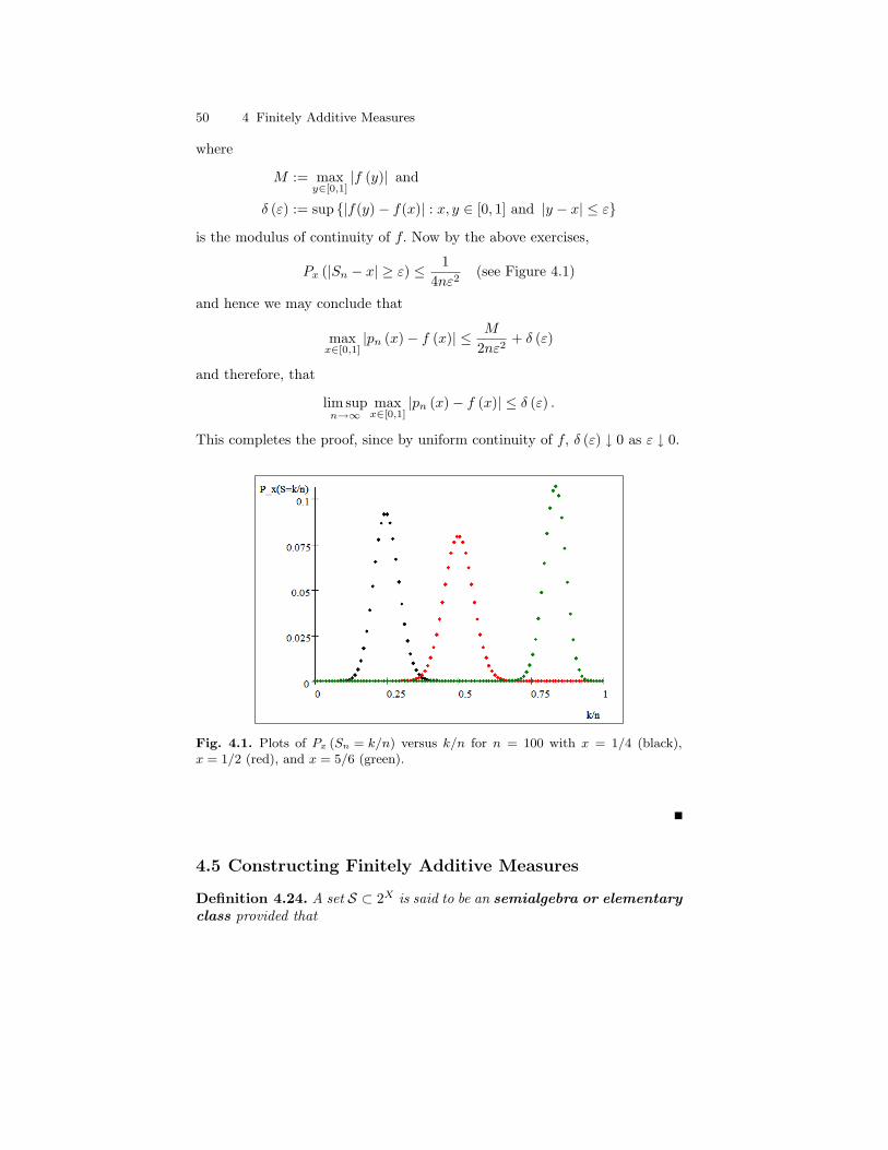
Px (|Sn − x| ≥ ε) ≤ 14nε2
(see Figure 4.1)
and hence we may conclude that
maxx∈[0,1]
|pn (x)− f (x)| ≤ M
2nε2+ δ (ε)
and therefore, that
lim supn→∞
maxx∈[0,1]
|pn (x)− f (x)| ≤ δ (ε) .
This completes the proof, since by uniform continuity of f, δ (ε) ↓ 0 as ε ↓ 0.
Fig. 4.1. Plots of Px (Sn = k/n) versus k/n for n = 100 with x = 1/4 (black),x = 1/2 (red), and x = 5/6 (green).
4.5 Constructing Finitely Additive Measures
Definition 4.24. A set S ⊂ 2X is said to be an semialgebra or elementaryclass provided that

4.5 Constructing Finitely Additive Measures 51
• ∅ ∈ S• S is closed under finite intersections• if E ∈ S, then Ec is a finite disjoint union of sets from S. (In particular
X = ∅c is a finite disjoint union of elements from S.)
Example 4.25. Let X = R, then
S :=(a, b] ∩ R : a, b ∈ R
= (a, b] : a ∈ [−∞,∞) and a < b <∞ ∪ ∅,R
is a semi-field
Exercise 4.5. Let A ⊂ 2X and B ⊂ 2Y be semi-fields. Show the collection
E := A×B : A ∈ A and B ∈ B
is also a semi-field.
Proposition 4.26. Suppose S ⊂ 2X is a semi-field, then A = A(S) consistsof sets which may be written as finite disjoint unions of sets from S.
Proof. Let A denote the collection of sets which may be written as finitedisjoint unions of sets from S. Clearly S ⊂ A ⊂ A(S) so it suffices to show A isan algebra since A(S) is the smallest algebra containing S. By the propertiesof S, we know that ∅, X ∈ A. Now suppose that Ai =
∑F∈Λi
F ∈ A where,for i = 1, 2, . . . , n, Λi is a finite collection of disjoint sets from S. Then
n⋂i=1
Ai =n⋂
i=1
(∑F∈Λi
F
)=
⋃(F1,,...,Fn)∈Λ1×···×Λn
(F1 ∩ F2 ∩ · · · ∩ Fn)
and this is a disjoint (you check) union of elements from S. Therefore A isclosed under finite intersections. Similarly, if A =
∑F∈Λ F with Λ being a
finite collection of disjoint sets from S, then Ac =⋂
F∈Λ Fc. Since by assump-
tion F c ∈ A for F ∈ Λ ⊂ S and A is closed under finite intersections, itfollows that Ac ∈ A.
Example 4.27. Let X = R and S :=(a, b] ∩ R : a, b ∈ R
be as in Example
4.25. Then A(S) may be described as being those sets which are finite disjointunions of sets from S.
Proposition 4.28 (Construction of Finitely Additive Measures). Sup-pose S ⊂ 2X is a semi-algebra (see Definition 4.24) and A = A(S) is thealgebra generated by S. Then every additive function µ : S → [0,∞] such thatµ (∅) = 0 extends uniquely to an additive measure (which we still denote byµ) on A.

52 4 Finitely Additive Measures
Proof. Since (by Proposition 4.26) every element A ∈ A is of the formA =
∑iEi for a finite collection of Ei ∈ S, it is clear that if µ extends to a
measure then the extension is unique and must be given by
µ(A) =∑
i
µ(Ei). (4.19)
To prove existence, the main point is to show that µ(A) in Eq. (4.19) is welldefined; i.e. if we also have A =
∑j Fj with Fj ∈ S, then we must show∑
i
µ(Ei) =∑
j
µ(Fj). (4.20)
But Ei =∑
j (Ei ∩ Fj) and the additivity of µ on S implies µ(Ei) =∑
j µ(Ei∩Fj) and hence∑
i
µ(Ei) =∑
i
∑j
µ(Ei ∩ Fj) =∑i,j
µ(Ei ∩ Fj).
Similarly, ∑j
µ(Fj) =∑i,j
µ(Ei ∩ Fj)
which combined with the previous equation shows that Eq. (4.20) holds. Itis now easy to verify that µ extended to A as in Eq. (4.19) is an additivemeasure on A.
Proposition 4.29. Let X = R, S be a semi-algebra
S = (a, b] ∩ R : −∞ ≤ a ≤ b ≤ ∞, (4.21)
and A = A(S) be the algebra formed by taking finite disjoint unions of ele-ments from S, see Proposition 4.26. To each finitely additive probability mea-sures µ : A → [0,∞], there is a unique increasing function F : R → [0, 1] suchthat F (−∞) = 0, F (∞) = 1 and
µ((a, b] ∩ R) = F (b)− F (a) ∀ a ≤ b in R. (4.22)
Conversely, given an increasing function F : R → [0, 1] such that F (−∞) = 0,F (∞) = 1 there is a unique finitely additive measure µ = µF on A such thatthe relation in Eq. (4.22) holds.
Proof. Given a finitely additive probability measure µ, let
F (x) := µ ((−∞, x] ∩ R) for all x ∈ R.
Then F (∞) = 1, F (−∞) = 0 and for b > a,
F (b)− F (a) = µ ((−∞, b] ∩ R)− µ ((−∞, a]) = µ ((a, b] ∩ R) .

4.5 Constructing Finitely Additive Measures 53
Conversely, suppose F : R → [0, 1] as in the statement of the theorem isgiven. Define µ on S using the formula in Eq. (4.22). The argument will becompleted by showing µ is additive on S and hence, by Proposition 4.28, hasa unique extension to a finitely additive measure on A. Suppose that
(a, b] =n∑
i=1
(ai, bi].
By reordering (ai, bi] if necessary, we may assume that
a = a1 < b1 = a2 < b2 = a3 < · · · < bn−1 = an < bn = b.
Therefore, by the telescoping series argument,
µ((a, b] ∩ R) = F (b)− F (a) =n∑
i=1
[F (bi)− F (ai)] =n∑
i=1
µ((ai, bi] ∩ R).


5
Countably Additive Measures
5.1 Distribution Function for Probability Measures on(R, BR)
Definition 5.1. Given a probability measure, P on BR, the cumulative dis-tribution function (CDF) of P is defined as the function, F = FP :R → [0, 1] given as
F (x) := P ((−∞, x]) .
Example 5.2. Suppose that
P = pδ−1 + qδ1 + rδπ
with p, q, r > 0 and p+ q + r = 1. In this case,
F (x) =
0 for x < −1p for −1 ≤ x < 1
p+ q for 1 ≤ x < π1 for π ≤ x <∞
.
Lemma 5.3. If F = FP : R → [0, 1] is a distribution function for a probabilitymeasure, P, on BR, then:
1. F (−∞) := limx→−∞ F (x) = 0,2. F (∞) := limx→∞ F (x) = 1,3. F is non-decreasing, and4. F is right continuous.
Theorem 5.4. To each function F : R → [0, 1] satisfying properties 1. – 4. inLemma 5.3, there exists a unique probability measure, PF , on BR such that
PF ((a, b]) = F (b)− F (a) for all −∞ < a ≤ b <∞.
Proof. The uniqueness assertion in the theorem is covered in Exercise 5.1below. The existence portion of the Theorem follows from Proposition 5.7 andTheorem 5.19 below.
Example 5.5 (Uniform Distribution). The function,

56 5 Countably Additive Measures
F (x) :=
0 for x ≤ 0x for 0 ≤ x < 11 for 1 ≤ x <∞
,
is the distribution function for a measure, m on BR which is concentratedon (0, 1]. The measure, m is called the uniform distribution or Lebesguemeasure on (0, 1].
Recall from Definition 3.14 that B ⊂ 2X is a σ – algebra on X if B is analgebra which is closed under countable unions and intersections.
5.2 Construction of Premeasures
Proposition 5.6. Suppose that S ⊂ 2X is a semi-algebra, A = A(S) andµ : A → [0,∞] is a finitely additive measure. Then µ is a premeasure on Aiff µ is sub-additive on S.
Proof. Clearly if µ is a premeasure on A then µ is σ - additive and hencesub-additive on S. Because of Proposition 4.2, to prove the converse it sufficesto show that the sub-additivity of µ on S implies the sub-additivity of µ onA.
So suppose A =∞∑
n=1An with A ∈ A and each An ∈ A which we express
as A =∑k
j=1Ej with Ej ∈ S and An =∑Nn
i=1En,i with En,i ∈ S. Then
Ej = A ∩ Ej =∞∑
n=1
An ∩ Ej =∞∑
n=1
Nn∑i=1
En,i ∩ Ej
which is a countable union and hence by assumption,
µ(Ej) ≤∞∑
n=1
Nn∑i=1
µ (En,i ∩ Ej) .
Summing this equation on j and using the finite additivity of µ shows
µ(A) =k∑
j=1
µ(Ej) ≤k∑
j=1
∞∑n=1
Nn∑i=1
µ (En,i ∩ Ej)
=∞∑
n=1
Nn∑i=1
k∑j=1
µ (En,i ∩ Ej) =∞∑
n=1
Nn∑i=1
µ (En,i) =∞∑
n=1
µ (An) ,
which proves (using Proposition 4.2) the sub-additivity of µ on A.Now suppose that F : R → R be an increasing function, F (±∞) :=
limx→±∞ F (x) and µ = µF be the finitely additive measure on (R,A) de-scribed in Proposition 4.29. If µ happens to be a premeasure on A, then,letting An = (a, bn] with bn ↓ b as n→∞, implies

5.2 Construction of Premeasures 57
F (bn)− F (a) = µ((a, bn]) ↓ µ((a, b]) = F (b)− F (a).
Since bn∞n=1 was an arbitrary sequence such that bn ↓ b, we have shownlimy↓b F (y) = F (b), i.e. F is right continuous. The next proposition shows theconverse is true as well. Hence premeasures on A which are finite on boundedsets are in one to one correspondences with right continuous increasing func-tions which vanish at 0.
Proposition 5.7. To each right continuous increasing function F : R → Rthere exists a unique premeasure µ = µF on A such that
µF ((a, b]) = F (b)− F (a) ∀ −∞ < a < b <∞.
Proof. As above, let F (±∞) := limx→±∞ F (x) and µ = µF be as inProposition 4.29. Because of Proposition 5.6, to finish the proof it suffices toshow µ is sub-additive on S.
First suppose that −∞ < a < b < ∞, J = (a, b], Jn = (an, bn] such that
J =∞∑
n=1Jn. We wish to show
µ(J) ≤∞∑
n=1
µ(Jn). (5.1)
To do this choose numbers a > a, bn > bn in which case I := (a, b] ⊂ J,
Jn := (an, bn] ⊃ Jon := (an, bn) ⊃ Jn.
Since I = [a, b] is compact and I ⊂ J ⊂∞⋃
n=1Jo
n there exists1 N <∞ such that
I ⊂ I ⊂N⋃
n=1
Jon ⊂
N⋃n=1
Jn.
Hence by finite sub-additivity of µ,
F (b)− F (a) = µ(I) ≤N∑
n=1
µ(Jn) ≤∞∑
n=1
µ(Jn).
Using the right continuity of F and letting a ↓ a in the above inequality,
1 To see this, let c := supn
x ≤ b : [a, x] is finitely covered byn
Jon
o∞n=1
o. If c < b,
then c ∈ Jom for some m and there exists x ∈ Jo
m such that [a, x] is finitely covered
byn
Jon
o∞n=1
, say byn
Jon
oN
n=1. We would then have that
nJo
n
omax(m,N)
n=1finitely
covers [a, c′] for all c′ ∈ Jom. But this contradicts the definition of c.
58 5 Countably Additive Measures
µ (J) = µ((a, b]) = F (b)− F (a) ≤∞∑
n=1
µ(Jn
)=∞∑
n=1
µ (Jn) +∞∑
n=1
µ(Jn \ Jn). (5.2)
Given ε > 0, we may use the right continuity of F to choose bn so that
µ(Jn \ Jn) = F (bn)− F (bn) ≤ ε2−n ∀ n ∈ N.
Using this in Eq. (5.2) shows
µ(J) = µ((a, b]) ≤∞∑
n=1
µ (Jn) + ε
which verifies Eq. (5.1) since ε > 0 was arbitrary.The hard work is now done but we still have to check the cases where
a = −∞ or b = ∞. For example, suppose that b = ∞ so that
J = (a,∞) =∞∑
n=1
Jn
with Jn = (an, bn] ∩ R. Then
IM := (a,M ] = J ∩ IM =∞∑
n=1
Jn ∩ IM
and so by what we have already proved,
F (M)− F (a) = µ(IM ) ≤∞∑
n=1
µ(Jn ∩ IM ) ≤∞∑
n=1
µ(Jn).
Now let M →∞ in this last inequality to find that
µ((a,∞)) = F (∞)− F (a) ≤∞∑
n=1
µ(Jn).
The other cases where a = −∞ and b ∈ R and a = −∞ and b = ∞ arehandled similarly.
Before continuing our development of the existence of measures, we willpause to show that measures are often uniquely determined by their valueson a generating sub-algebra. This detour will also have the added benefit ofmotivating Carathoedory’s existence proof to be given below.

5.3 Regularity and Uniqueness Results 59
5.3 Regularity and Uniqueness Results
Definition 5.8. Given a collection of subsets, E , of X, let Eσ denote the col-lection of subsets of X which are finite or countable unions of sets from E .Similarly let Eδ denote the collection of subsets of X which are finite or count-able intersections of sets from E . We also write Eσδ = (Eσ)δ and Eδσ = (Eδ)σ ,etc.
Lemma 5.9. Suppose that A ⊂ 2X is an algebra. Then:
1. Aσ is closed under taking countable unions and finite intersections.2. Aδ is closed under taking countable intersections and finite unions.3. Ac : A ∈ Aσ = Aδ and Ac : A ∈ Aδ = Aσ.
Proof. By construction Aσ is closed under countable unions. Moreover ifA = ∪∞i=1Ai and B = ∪∞j=1Bj with Ai, Bj ∈ A, then
A ∩B = ∪∞i,j=1Ai ∩Bj ∈ Aσ,
which shows that Aσ is also closed under finite intersections. Item 3. is straightforward and item 2. follows from items 1. and 3.
Theorem 5.10 (Finite Regularity Result). Suppose A ⊂ 2X is an al-gebra, B = σ (A) and µ : B → [0,∞) is a finite measure, i.e. µ (X) < ∞.Then for every ε > 0 and B ∈ B there exists A ∈ Aδ and C ∈ Aσ such thatA ⊂ B ⊂ C and µ (C \A) < ε.
Proof. Let B0 denote the collection of B ∈ B such that for every ε > 0there here exists A ∈ Aδ and C ∈ Aσ such that A ⊂ B ⊂ C and µ (C \A) < ε.It is now clear that A ⊂ B0 and that B0 is closed under complementation. Nowsuppose that Bi ∈ B0 for i = 1, 2, . . . and ε > 0 is given. By assumption thereexists Ai ∈ Aδ and Ci ∈ Aσ such that Ai ⊂ Bi ⊂ Ci and µ (Ci \Ai) < 2−iε.
Let A := ∪∞i=1Ai, AN := ∪N
i=1Ai ∈ Aδ, B := ∪∞i=1Bi, and C := ∪∞i=1Ci ∈Aσ. Then AN ⊂ A ⊂ B ⊂ C and
C \A = [∪∞i=1Ci] \A = ∪∞i=1 [Ci \A] ⊂ ∪∞i=1 [Ci \Ai] .
Therefore,
µ (C \A) = µ (∪∞i=1 [Ci \A]) ≤∞∑
i=1
µ (Ci \A) ≤∞∑
i=1
µ (Ci \Ai) < ε.
Since C \AN ↓ C \A, it also follows that µ(C \AN
)< ε for sufficiently large
N and this shows B = ∪∞i=1Bi ∈ B0. Hence B0 is a sub-σ-algebra of B = σ (A)which contains A which shows B0 = B.
Many theorems in the sequel will require some control on the size of ameasure µ. The relevant notion for our purposes (and most purposes) is thatof a σ – finite measure defined next.

60 5 Countably Additive Measures
Definition 5.11. Suppose X is a set, E ⊂ B ⊂ 2X and µ : B → [0,∞] is afunction. The function µ is σ – finite on E if there exists En ∈ E such thatµ(En) <∞ and X = ∪∞n=1En. If B is a σ – algebra and µ is a measure on Bwhich is σ – finite on B we will say (X,B, µ) is a σ – finite measure space.
The reader should check that if µ is a finitely additive measure on analgebra, B, then µ is σ – finite on B iff there exists Xn ∈ B such that Xn ↑ Xand µ(Xn) <∞.
Corollary 5.12 (σ – Finite Regularity Result). Theorem 5.10 continuesto hold under the weaker assumption that µ : B → [0,∞] is a measure whichis σ – finite on A.
Proof. LetXn ∈ A such that ∪∞n=1Xn = X and µ(Xn) <∞ for all n.SinceA ∈ B →µn (A) := µ (Xn ∩A) is a finite measure on A ∈ B for each n, byTheorem 5.10, for every B ∈ B there exists Cn ∈ Aσ such that B ⊂ Cn andµ (Xn ∩ [Cn \B]) = µn (Cn \B) < 2−nε. Now let C := ∪∞n=1 [Xn ∩ Cn] ∈ Aσ
and observe that B ⊂ C and
µ (C \B) = µ (∪∞n=1 ([Xn ∩ Cn] \B))
≤∞∑
n=1
µ ([Xn ∩ Cn] \B) =∞∑
n=1
µ (Xn ∩ [Cn \B]) < ε.
Applying this result to Bc shows there exists D ∈ Aσ such that Bc ⊂ D and
µ (B \Dc) = µ (D \Bc) < ε.
So if we let A := Dc ∈ Aδ, then A ⊂ B ⊂ C and
µ (C \A) = µ ([B \A] ∪ [(C \B) \A]) ≤ µ (B \A) + µ (C \B) < 2ε
and the result is proved.
Exercise 5.1. Suppose A ⊂ 2X is an algebra and µ and ν are two measureson B = σ (A) .
a. Suppose that µ and ν are finite measures such that µ = ν on A. Showµ = ν.
b. Generalize the previous assertion to the case where you only assume thatµ and ν are σ – finite on A.
Corollary 5.13. Suppose A ⊂ 2X is an algebra and µ : B = σ (A) → [0,∞] isa measure which is σ – finite on A. Then for all B ∈ B, there exists A ∈ Aδσ
and C ∈ Aσδ such that A ⊂ B ⊂ C and µ (C \A) = 0.
Proof. By Theorem 5.10, given B ∈ B, we may choose An ∈ Aδ andCn ∈ Aσ such that An ⊂ B ⊂ Cn and µ(Cn \B) ≤ 1/n and µ(B \An) ≤ 1/n.By replacing AN by ∪N
n=1An and CN by ∩Nn=1Cn, we may assume that An ↑

5.4 Construction of Measures 61
and Cn ↓ as n increases. Let A = ∪An ∈ Aδσ and C = ∩Cn ∈ Aσδ, thenA ⊂ B ⊂ C and
µ(C \A) = µ(C \B) + µ(B \A) ≤ µ(Cn \B) + µ(B \An)≤ 2/n→ 0 as n→∞.
Exercise 5.2. Let B = BRn = σ (open subsets of Rn) be the Borel σ –algebra on Rn and µ be a probability measure on B. Further, let B0 denotethose sets B ∈ B such that for every ε > 0 there exists F ⊂ B ⊂ V such thatF is closed, V is open, and µ (V \ F ) < ε. Show:
1. B0 contains all closed subsets of B. Hint: given a closed subset,F ⊂ Rn and k ∈ N, let Vk := ∪x∈FB (x, 1/k) , where B (x, δ) :=y ∈ Rn : |y − x| < δ . Show, Vk ↓ F as k →∞.
2. Show B0 is a σ – algebra and use this along with the first part of thisexercise to conclude B = B0. Hint: follow closely the method used in thefirst step of the proof of Theorem 5.10.
3. Show for every ε > 0 and B ∈ B, there exist a compact subset,K ⊂ Rn, such that K ⊂ B and µ (B \K) < ε. Hint: take K :=F ∩ x ∈ Rn : |x| ≤ n for some sufficiently large n.
5.4 Construction of Measures
Remark 5.14. Let us recall from Proposition 4.3 and Remark 4.4 that a finitelyadditive measure µ : A → [0,∞] is a premeasure on A iff µ (An) ↑ µ(A) forall An∞n=1 ⊂ A such that An ↑ A ∈ A. Furthermore if µ (X) <∞, then µ isa premeasure on A iff µ(An) ↓ 0 for all An∞n=1 ⊂ A such that An ↓ ∅.
Proposition 5.15. Let µ be a premeasure on an algebra A, then µ has aunique extension (still called µ) to a function on Aσ satisfying the followingproperties.
1. (Continuity) If An ∈ A and An ↑ A ∈ Aσ, then µ (An) ↑ µ (A) asn→∞.
2. (Monotonicity) If A,B ∈ Aσ with A ⊂ B then µ (A) ≤ µ (B) .3. (Strong Additivity) If A,B ∈ Aσ, then
µ (A ∪B) + µ (A ∩B) = µ (A) + µ (B) . (5.3)
4. (Sub-Additivity on Aσ) The function µ is sub-additive on Aσ, i.e. ifAn∞n=1 ⊂ Aσ, then
µ (∪∞n=1An) ≤∞∑
n=1
µ (An) . (5.4)

62 5 Countably Additive Measures
5. (σ - Additivity on Aσ) The function µ is countably additive on Aσ.
Proof. Let A,B be sets in Aσ such that A ⊂ B and suppose An∞n=1
and Bn∞n=1 are sequences in A such that An ↑ A and Bn ↑ B as n → ∞.Since Bm ∩An ↑ An as m→∞, the continuity of µ on A implies,
µ (An) = limm→∞
µ (Bm ∩An) ≤ limm→∞
µ (Bm) .
We may let n→∞ in this inequality to find,
limn→∞
µ (An) ≤ limm→∞
µ (Bm) . (5.5)
Using this equation when B = A, implies, limn→∞ µ (An) = limm→∞ µ (Bm)whenever An ↑ A and Bn ↑ A. Therefore it is unambiguous to define µ (A)by;
µ (A) = limn→∞
µ (An)
for any sequence An∞n=1 ⊂ A such that An ↑ A. With this definition, thecontinuity of µ is clear and the monotonicity of µ follows from Eq. (5.5).
Suppose that A,B ∈ Aσ and An∞n=1 and Bn∞n=1 are sequences in Asuch that An ↑ A and Bn ↑ B as n→∞. Then passing to the limit as n→∞in the identity,
µ (An ∪Bn) + µ (An ∩Bn) = µ (An) + µ (Bn)
proves Eq. (5.3). In particular, it follows that µ is finitely additive on Aσ.Let An∞n=1 be any sequence in Aσ and choose An,i∞i=1 ⊂ A such that
An,i ↑ An as i→∞. Then we have,
µ(∪N
n=1An,N
)≤
N∑n=1
µ (An,N ) ≤N∑
n=1
µ (An) ≤∞∑
n=1
µ (An) . (5.6)
Since A 3 ∪Nn=1An,N ↑ ∪∞n=1An ∈ Aσ, we may let N → ∞ in Eq. (5.6) to
conclude Eq. (5.4) holds.If we further assume that An∞n=1 ⊂ Aσ is a disjoint sequence, by the
finite additivity and monotonicity of µ on Aσ, we have
∞∑n=1
µ (An) = limN→∞
N∑n=1
µ (An) = limN→∞
µ(∪N
n=1An
)≤ µ (∪∞n=1An) .
The previous two inequalities show µ is σ – additive on Aσ.Suppose µ is a finite premeasure on an algebra, A ⊂ 2X , and A ∈ Aδ∩Aσ.
Since A,Ac ∈ Aσ and X = A ∪ Ac, it follows that µ (X) = µ (A) + µ (Ac) .From this observation we may extend µ to a function on Aδ ∪Aσ by defining
µ (A) := µ (X)− µ (Ac) for all A ∈ Aδ. (5.7)
5.4 Construction of Measures 63
Lemma 5.16. Suppose µ is a finite premeasure on an algebra, A ⊂ 2X , andµ has been extended to Aδ∪Aσ as described in Proposition 5.15 and Eq. (5.7)above.
1. If A ∈ Aδ and An ∈ A such that An ↓ A, then µ (A) = limn→∞ µ (An) .2. µ is additive when restricted to Aδ.3. If A ∈ Aδ and C ∈ Aσ such that A ⊂ C, then µ (C \A) = µ (C)− µ (A) .
Proof.
1. Since Acn ↑ Ac ∈ Aσ, by the definition of µ (A) and Proposition 5.15 it
follows that
µ (A) = µ (X)− µ (Ac) = µ (X)− limn→∞
µ (Acn)
= limn→∞
[µ (X)− µ (Acn)] = lim
n→∞µ (An) .
2. Suppose A,B ∈ Aδ are disjoint sets and An, Bn ∈ A such that An ↓ Aand Bn ↓ B, then An ∪Bn ↓ A ∪B and therefore,
µ (A ∪B) = limn→∞
µ (An ∪Bn) = limn→∞
[µ (An) + µ (Bn)− µ (An ∩Bn)]
= µ (A) + µ (B)
wherein the last equality we have used Proposition 4.3.3. By assumption, X = Ac ∪ C. So applying the strong additivity of µ onAσ in Eq. (5.3) with A→ Ac ∈ Aσ and B → C ∈ Aσ shows
µ (X) + µ (C \A) = µ (Ac ∪ C) + µ (Ac ∩ C)= µ (Ac) + µ (C) = µ (X)− µ (A) + µ (C) .
Definition 5.17 (Measurable Sets). Suppose µ is a finite premeasure onan algebra A ⊂ 2X . We say that B ⊂ X is measurable if for all ε > 0 thereexists A ∈ Aδ and C ∈ Aσ such that A ⊂ B ⊂ C and µ (C \A) < ε. We willdenote the collection of measurable subsets of X by B = B (µ) . We also defineµ : B → [0, µ (X)] by
µ (B) = inf µ (C) : B ⊂ C ∈ Aσ . (5.8)
Remark 5.18. If B ∈ B, ε > 0, A ∈ Aδ and C ∈ Aσ are such that A ⊂ B ⊂ Cand µ (C \A) < ε, then µ (A) ≤ µ (B) ≤ µ (C) and in particular,
0 ≤ µ (B)− µ (A) < ε, and 0 ≤ µ (C)− µ (B) < ε. (5.9)
Indeed, if C ′ ∈ Aσ with B ⊂ C ′, then A ⊂ C ′ and so by Lemma 5.16,
µ (A) ≤ µ (C ′ \A) + µ (A) = µ (C ′)
from which it follows that µ (A) ≤ µ (B) . The fact that µ (B) ≤ µ (C) followsdirectly from Eq. (5.8).
64 5 Countably Additive Measures
Theorem 5.19 (Finite Premeasure Extension Theorem). Suppose µ isa finite premeasure on an algebra A ⊂ 2X . Then B is a σ – algebra on Xwhich contains A and µ is a σ – additive measure on B. Moreover, µ is theunique measure on B such that µ|A = µ.
Proof. It is clear that A ⊂ B and that B is closed under complementation.Now suppose that Bi ∈ B for i = 1, 2 and ε > 0 is given. We may thenchoose Ai ⊂ Bi ⊂ Ci such that Ai ∈ Aδ, Ci ∈ Aσ, and µ (Ci \Ai) < ε fori = 1, 2. Then with A = A1 ∪ A2, B = B1 ∪ B2 and C = C1 ∪ C2, we haveAδ 3 A ⊂ B ⊂ C ∈ Aσ. Since
C \A = (C1 \A) ∪ (C2 \A) ⊂ (C1 \A1) ∪ (C2 \A2) ,
it follows from the sub-additivity of µ that with
µ (C \A) ≤ µ (C1 \A1) + µ (C2 \A2) < 2ε.
Since ε > 0 was arbitrary, we have shown that B ∈ B. Hence we now knowthat B is an algebra.
Because B is an algebra, to verify that B is a σ – algebra it suffices toshow that B =
∑∞n=1Bn ∈ B whenever Bn∞n=1 is a disjoint sequence in
B. To prove B ∈ B, let ε > 0 be given and choose Ai ⊂ Bi ⊂ Ci such thatAi ∈ Aδ, Ci ∈ Aσ, and µ (Ci \Ai) < ε2−i for all i. Since the Ai∞i=1 arepairwise disjoint we may use Lemma 5.16 to show,
n∑i=1
µ (Ci) =n∑
i=1
(µ (Ai) + µ (Ci \Ai))
= µ (∪ni=1Ai) +
n∑i=1
µ (Ci \Ai) ≤ µ (X) +n∑
i=1
ε2−i.
Passing to the limit, n→∞, in this equation then shows∞∑
i=1
µ (Ci) ≤ µ (X) + ε <∞. (5.10)
Let B = ∪∞i=1Bi, C := ∪∞i=1Ci ∈ Aσ and for n ∈ N let An :=∑n
i=1Ai ∈Aδ. Then Aδ 3 An ⊂ B ⊂ C ∈ Aσ, C \An ∈ Aσ and
C \An = ∪∞i=1 (Ci \An) ⊂ [∪ni=1 (Ci \Ai)] ∪
[∪∞i=n+1Ci
]∈ Aσ.
Therefore, using the sub-additivity of µ on Aσ and the estimate (5.10),
µ (C \An) ≤n∑
i=1
µ (Ci \Ai) +∞∑
i=n+1
µ (Ci)
≤ ε+∞∑
i=n+1
µ (Ci) → ε as n→∞.

5.4 Construction of Measures 65
Since ε > 0 is arbitrary, it follows that B ∈ B. Moreover by repeated use ofRemark 5.18, we find
|µ (B)− µ (An)| < ε+∞∑
i=n+1
µ (Ci) and∣∣∣∣∣n∑
i=1
µ (Bi)− µ (An)
∣∣∣∣∣ =∣∣∣∣∣
n∑i=1
[µ (Bi)− µ (Ai)]
∣∣∣∣∣ ≤n∑
i=1
|µ (Bi)− µ (Ai)| ≤ εn∑
i=1
2−i < ε.
Combining these estimates shows∣∣∣∣∣µ (B)−n∑
i=1
µ (Bi)
∣∣∣∣∣ < 2ε+∞∑
i=n+1
µ (Ci)
which upon letting n→∞ gives,∣∣∣∣∣µ (B)−∞∑
i=1
µ (Bi)
∣∣∣∣∣ ≤ 2ε.
Since ε > 0 is arbitrary, we have shown µ (B) =∑∞
i=1 µ (Bi) . This completesthe proof that B is a σ - algebra and that µ is a measure on B.
Theorem 5.20. Suppose that µ is a σ – finite premeasure on an algebra A.Then
µ (B) := inf µ (C) : B ⊂ C ∈ Aσ ∀ B ∈ σ (A) (5.11)
defines a measure on σ (A) and this measure is the unique extension of µ onA to a measure on σ (A) .
Proof. Let Xn∞n=1 ⊂ A be chosen so that µ (Xn) < ∞ for all n andXn ↑ X as n→∞ and let
µn (A) := µn (A ∩Xn) for all A ∈ A.
Each µn is a premeasure (as is easily verified) on A and hence by Theorem5.19 each µn has an extension, µn, to a measure on σ (A) . Since the measureµn are increasing, µ := limn→∞ µn is a measure which extends µ.
The proof will be completed by verifying that Eq. (5.11) holds. Let B ∈σ (A) , Bm = Xm ∩ B and ε > 0 be given. By Theorem 5.19, there existsCm ∈ Aσ such that Bm ⊂ Cm ⊂ Xm and µ(Cm\Bm) = µm(Cm\Bm) < ε2−n.Then C := ∪∞m=1Cm ∈ Aσ and
µ(C \B) ≤ µ
( ∞⋃m=1
(Cm \B)
)≤∞∑
m=1
µ(Cm \B) ≤∞∑
m=1
µ(Cm \Bm) < ε.
Thusµ (B) ≤ µ (C) = µ (B) + µ(C \B) ≤ µ (B) + ε
which, since ε > 0 is arbitrary, shows µ satisfies Eq. (5.11). The uniquenessof the extension µ is proved in Exercise 5.1.
66 5 Countably Additive Measures
Example 5.21. If F (x) = x for all x ∈ R, we denote µF by m and call mLebesgue measure on (R,BR) .
Theorem 5.22. Lebesgue measure m is invariant under translations, i.e. forB ∈ BR and x ∈ R,
m(x+B) = m(B). (5.12)
Moreover, m is the unique measure on BR such that m((0, 1]) = 1 and Eq.(5.12) holds for B ∈ BR and x ∈ R. Moreover, m has the scaling property
m(λB) = |λ|m(B) (5.13)
where λ ∈ R, B ∈ BR and λB := λx : x ∈ B.Proof. Let mx(B) := m(x + B), then one easily shows that mx is a
measure on BR such that mx((a, b]) = b− a for all a < b. Therefore, mx = mby the uniqueness assertion in Exercise 5.1. For the converse, suppose that mis translation invariant and m((0, 1]) = 1. Given n ∈ N, we have
(0, 1] = ∪nk=1(
k − 1n
,k
n] = ∪n
k=1
(k − 1n
+ (0,1n
]).
Therefore,
1 = m((0, 1]) =n∑
k=1
m
(k − 1n
+ (0,1n
])
=n∑
k=1
m((0,1n
]) = n ·m((0,1n
]).
That is to say
m((0,1n
]) = 1/n.
Similarly, m((0, ln ]) = l/n for all l, n ∈ N and therefore by the translation
invariance of m,
m((a, b]) = b− a for all a, b ∈ Q with a < b.
Finally for a, b ∈ R such that a < b, choose an, bn ∈ Q such that bn ↓ b andan ↑ a, then (an, bn] ↓ (a, b] and thus
m((a, b]) = limn→∞
m((an, bn]) = limn→∞
(bn − an) = b− a,
i.e. m is Lebesgue measure. To prove Eq. (5.13) we may assume that λ 6= 0since this case is trivial to prove. Now let mλ(B) := |λ|−1
m(λB). It is easilychecked that mλ is again a measure on BR which satisfies
mλ((a, b]) = λ−1m ((λa, λb]) = λ−1(λb− λa) = b− a
if λ > 0 and
mλ((a, b]) = |λ|−1m ([λb, λa)) = − |λ|−1 (λb− λa) = b− a
if λ < 0. Hence mλ = m.

5.5 Completions of Measure Spaces 67
5.5 Completions of Measure Spaces
Definition 5.23. A set E ⊂ X is a null set if E ∈ B and µ(E) = 0. If P issome “property” which is either true or false for each x ∈ X, we will use theterminology P a.e. (to be read P almost everywhere) to mean
E := x ∈ X : P is false for x
is a null set. For example if f and g are two measurable functions on (X,B, µ),f = g a.e. means that µ(f 6= g) = 0.
Definition 5.24. A measure space (X,B, µ) is complete if every subset ofa null set is in B, i.e. for all F ⊂ X such that F ⊂ E ∈ B with µ(E) = 0implies that F ∈ B.
Proposition 5.25 (Completion of a Measure). Let (X,B, µ) be a measurespace. Set
N = N µ := N ⊂ X : ∃ F ∈ B such that N ⊂ F and µ(F ) = 0 ,B = Bµ := A ∪N : A ∈ B and N ∈ N and
µ(A ∪N) := µ(A) for A ∈ B and N ∈ N ,
see Fig. 5.1. Then B is a σ – algebra, µ is a well defined measure on B, µis the unique measure on B which extends µ on B, and (X, B, µ) is completemeasure space. The σ-algebra, B, is called the completion of B relative to µand µ, is called the completion of µ.
Proof. Clearly X, ∅ ∈ B. Let A ∈ B and N ∈ N and choose F ∈ B such
Fig. 5.1. Completing a σ – algebra.
that N ⊂ F and µ(F ) = 0. Since N c = (F \N) ∪ F c,
(A ∪N)c = Ac ∩N c = Ac ∩ (F \N ∪ F c)= [Ac ∩ (F \N)] ∪ [Ac ∩ F c]

68 5 Countably Additive Measures
where [Ac ∩ (F \ N)] ∈ N and [Ac ∩ F c] ∈ B. Thus B is closed undercomplements. If Ai ∈ B and Ni ⊂ Fi ∈ B such that µ(Fi) = 0 then∪(Ai ∪ Ni) = (∪Ai) ∪ (∪Ni) ∈ B since ∪Ai ∈ B and ∪Ni ⊂ ∪Fi andµ(∪Fi) ≤
∑µ(Fi) = 0. Therefore, B is a σ – algebra. Suppose A∪N1 = B∪N2
with A,B ∈ B and N1, N2,∈ N . Then A ⊂ A ∪N1 ⊂ A ∪N1 ∪ F2 = B ∪ F2
which shows thatµ(A) ≤ µ(B) + µ(F2) = µ(B).
Similarly, we show that µ(B) ≤ µ(A) so that µ(A) = µ(B) and hence µ(A ∪N) := µ(A) is well defined. It is left as an exercise to show µ is a measure,i.e. that it is countable additive.
5.6 A Baby Version of Kolmogorov’s Extension Theorem
For this section, let Λ be a finite set, Ω := Λ∞ := ΛN, and let A denote thecollection of cylinder subsets of Ω, where A ⊂ Ω is a cylinder set iff thereexists n ∈ N and B ⊂ Λn such that
A = B × Λ∞ := ω ∈ Ω : (ω1, . . . , ωn) ∈ B .
Observe that we may also write A as A = B′×Λ∞ where B′ = B×Λk ⊂ Λn+k
for any k ≥ 0.
Exercise 5.3. Show A is an algebra.
Lemma 5.26. Suppose An∞n=1 ⊂ A is a decreasing sequence of non-emptycylinder sets, then ∩∞n=1An 6= ∅.
Proof. Since An ∈ A, we may find Nn ∈ N and Bn ⊂ ΛNn such thatAn = Bn × Λ∞. Using the observation just prior to this Lemma, we mayassume that Nn∞n=1 is a strictly increasing sequence.
By assumption, there exists ω (n) = (ω1 (n) , ω2 (n) , . . . ) ∈ Ω such thatω (n) ∈ An for all n. Moreover, since ω (n) ∈ An ⊂ Ak for all k ≤ n, it followsthat
(ω1 (n) , ω2 (n) , . . . , ωNk(n)) ∈ Bk for all k ≤ n. (5.14)
Since Λ is a finite set, we may find a λ1 ∈ Λ and an infinite subset, Γ1 ⊂ Nsuch that ω1 (n) = λ1 for all n ∈ Γ1. Similarly, there exists λ2 ∈ Λ and aninfinite set, Γ2 ⊂ Γ1, such that ω2 (n) = λ2 for all n ∈ Γ2. Continuing thisprocedure inductively, there exists (for all j ∈ N) infinite subsets, Γj ⊂ N andpoints λj ∈ Λ such that Γ1 ⊃ Γ2 ⊃ Γ3 ⊃ . . . and ωj (n) = λj for all n ∈ Γj .
We are now going to complete the proof by showing that λ := (λ1, λ2, . . . )is in ∩∞n=1An. By the construction above, for all N ∈ N we have
(ω1 (n) , . . . , ωN (n)) = (λ1, . . . , λN ) for all n ∈ ΓN .
Taking N = Nk and n ∈ ΓNkwith n ≥ k, we learn from Eq. (5.14) that

5.6 A Baby Version of Kolmogorov’s Extension Theorem 69
(λ1, . . . , λNk) = (ω1 (n) , . . . , ωNk
(n)) ∈ Bk.
But this is equivalent to showing λ ∈ Ak. Since k ∈ N was arbitrary it followsthat λ ∈ ∩∞n=1An.
Theorem 5.27 (Kolmogorov’s Extension Theorem I.). Continuing thenotation above, every finitely additive probability measure, P : A → [0, 1] , hasa unique extension to a probability measure on σ (A) .
Proof. From Theorem 5.19, it suffices to show limn→∞ P (An) = 0 when-ever An∞n=1 ⊂ A with An ↓ ∅. However, by Lemma 5.26, if An ∈ A andAn ↓ ∅, we must have that An = ∅ for a.a. n and in particular P (An) = 0 fora.a. n. This certainly implies limn→∞ P (An) = 0.
Given a probability measure, P : σ (A) → [0, 1] and n ∈ N and(λ1, . . . , λn) ∈ Λn, let
pn (λ1, . . . , λn) := P (ω ∈ Ω : ω1 = λ1, . . . , ωn = λn) . (5.15)
Exercise 5.4 (Consistency Conditions). If pn is defined as above, show:
1.∑
λ∈Λ p1 (λ) = 1 and2. for all n ∈ N and (λ1, . . . , λn) ∈ Λn,
pn (λ1, . . . , λn) =∑λ∈Λ
pn+1 (λ1, . . . , λn, λ) .
Exercise 5.5 (Converse to 5.4). Suppose for each n ∈ N we are givenfunctions, pn : Λn → [0, 1] such that the consistency conditions in Exercise5.4 hold. Then there exists a unique probability measure, P on σ (A) suchthat Eq. (5.15) holds for all n ∈ N and (λ1, . . . , λn) ∈ Λn.
Example 5.28 (Existence of iid simple R.V.s). Suppose now that q : Λ→ [0, 1]is a function such that
∑λ∈Λ q (λ) = 1. Then there exists a unique probability
measure P on σ (A) such that, for all n ∈ N and (λ1, . . . , λn) ∈ Λn, we have
P (ω ∈ Ω : ω1 = λ1, . . . , ωn = λn) = q (λ1) . . . q (λn) .
This is a special case of Exercise 5.5 with pn (λ1, . . . , λn) := q (λ1) . . . q (λn) .


6
Random Variables
6.1 Measurable Functions
Definition 6.1. A measurable space is a pair (X,M), where X is a setand M is a σ – algebra on X.
To motivate the notion of a measurable function, suppose (X,M, µ) is ameasure space and f : X → R+ is a function. Roughly speaking, we are goingto define
∫X
fdµ as a certain limit of sums of the form,
∞∑0<a1<a2<a3<...
aiµ(f−1(ai, ai+1]).
For this to make sense we will need to require f−1((a, b]) ∈ M for all a <b. Because of Corollary 6.7 below, this last condition is equivalent to thecondition f−1(BR) ⊂M.
Definition 6.2. Let (X,M) and (Y,F) be measurable spaces. A function f :X → Y is measurable of more precisely, M/F – measurable or (M,F) –measurable, if f−1(F) ⊂M, i.e. if f−1 (A) ∈M for all A ∈ F .
Remark 6.3. Let f : X → Y be a function. Given a σ – algebra F ⊂ 2Y , theσ – algebra M := f−1(F) is the smallest σ – algebra on X such that f is(M,F) - measurable . Similarly, if M is a σ - algebra on X then
F = f∗M =A ∈ 2Y |f−1(A) ∈M
is the largest σ – algebra on Y such that f is (M,F) - measurable.
Example 6.4 (Characteristic Functions). Let (X,M) be a measurable spaceand A ⊂ X. Then 1A is (M,BR) – measurable iff A ∈M. Indeed, 1−1
A (W ) iseither ∅, X, A or Ac for any W ⊂ R with 1−1
A (1) = A.
Example 6.5. Suppose f : X → Y with Y being a finite set and F = 2Ω . Thenf is measurable iff f−1 (y) ∈M for all y ∈ Y.
Proposition 6.6. Suppose that (X,M) and (Y,F) are measurable spaces andfurther assume E ⊂ F generates F , i.e. F = σ (E) . Then a map, f : X → Yis measurable iff f−1 (E) ⊂M.

72 6 Random Variables
Proof. If f isM/F measurable, then f−1 (E) ⊂ f−1 (F) ⊂M. Converselyif f−1 (E) ⊂M, then, using Lemma 3.26,
f−1 (F) = f−1 (σ (E)) = σ(f−1 (E)
)⊂M.
Corollary 6.7. Suppose that (X,M) is a measurable space. Then the follow-ing conditions on a function f : X → R are equivalent:
1. f is (M,BR) – measurable,2. f−1((a,∞)) ∈M for all a ∈ R,3. f−1((a,∞)) ∈M for all a ∈ Q,4. f−1((−∞, a]) ∈M for all a ∈ R.
Exercise 6.1. Prove Corollary 6.7. Hint: See Exercise 3.9.
Exercise 6.2. If M is the σ – algebra generated by E ⊂ 2X , then M is theunion of the σ – algebras generated by countable subsets F ⊂ E .
Exercise 6.3. Let (X,M) be a measure space and fn : X → R be a sequenceof measurable functions on X. Show that x : limn→∞ fn(x) exists in R ∈M.
Exercise 6.4. Show that every monotone function f : R → R is (BR,BR) –measurable.
Definition 6.8. Given measurable spaces (X,M) and (Y,F) and a subsetA ⊂ X. We say a function f : A → Y is measurable iff f is MA/F –measurable.
Proposition 6.9 (Localizing Measurability). Let (X,M) and (Y,F) bemeasurable spaces and f : X → Y be a function.
1. If f is measurable and A ⊂ X then f |A : A→ Y is measurable.2. Suppose there exist An ∈ M such that X = ∪∞n=1An and f |An is MAn
measurable for all n, then f is M – measurable.
Proof. 1. If f : X → Y is measurable, f−1(B) ∈ M for all B ∈ F andtherefore
f |−1A (B) = A ∩ f−1(B) ∈MA for all B ∈ F .
2. If B ∈ F , then
f−1(B) = ∪∞n=1
(f−1(B) ∩An
)= ∪∞n=1f |−1
An(B).
Since each An ∈M,MAn ⊂M and so the previous displayed equation showsf−1(B) ∈M.
The proof of the following exercise is routine and will be left to the reader.

6.1 Measurable Functions 73
Proposition 6.10. Let (X,M, µ) be a measure space, (Y,F) be a measurablespace and f : X → Y be a measurable map. Define a function ν : F → [0,∞]by ν(A) := µ(f−1(A)) for all A ∈ F . Then ν is a measure on (Y,F) . (In thefuture we will denote ν by f∗µ or µ f−1 and call f∗µ the push-forward ofµ by f or the law of f under µ.
Theorem 6.11. Given a distribution function, F : R → [0, 1] let G :(0, 1)→ R be defined (see Figure 6.1) by,
G (y) := inf x : F (x) ≥ y .
Then G : (0, 1)→ R is Borel measurable and G∗m = µF where µF is theunique measure on (R,BR) such that µF ((a, b]) = F (b)−F (a) for all −∞ <a < b <∞.
Fig. 6.1. A pictorial definition of G.
Proof. Since G : (0, 1) → R is a non-decreasing function, G is measurable.We also claim that, for all x0 ∈ R, that
G−1 ((0, x0]) = y : G (y) ≤ x0 = (0, F (x0)] ∩ R, (6.1)
see Figure 6.2.To give a formal proof of Eq. (6.1), G (y) = inf x : F (x) ≥ y ≤ x0, there
exists xn ≥ x0 with xn ↓ x0 such that F (xn) ≥ y. By the right continuity ofF, it follows that F (x0) ≥ y. Thus we have shown
G ≤ x0 ⊂ (0, F (x0)] ∩ (0, 1) .
For the converse, if y ≤ F (x0) then G (y) = inf x : F (x) ≥ y ≤ x0, i.e.y ∈ G ≤ x0 . Indeed, y ∈ G−1 ((−∞, x0]) iff G (y) ≤ x0. Observe that
G (F (x0)) = inf x : F (x) ≥ F (x0) ≤ x0

74 6 Random Variables
Fig. 6.2. As can be seen from this picture, G (y) ≤ x0 iff y ≤ F (x0) and similalry,G (y) ≤ x1 iff y ≤ x1.
and hence G (y) ≤ x0 whenever y ≤ F (x0) . This shows that
(0, F (x0)] ∩ (0, 1) ⊂ G−1 ((0, x0]) .
As a consequence we have G∗m = µF . Indeed,
(G∗m) ((−∞, x]) = m(G−1 ((−∞, x])
)= m (y ∈ (0, 1) : G (y) ≤ x)
= m ((0, F (x)] ∩ (0, 1)) = F (x) .
See section 2.5.2 on p. 61 of Resnick for more details.
Theorem 6.12 (Durret’s Version). Given a distribution function, F :R → [0, 1] let Y : (0, 1)→ R be defined (see Figure 6.3) by,
Y (x) := sup y : F (y) < x .
Then Y : (0, 1)→ R is Borel measurable and Y∗m = µF where µF is theunique measure on (R,BR) such that µF ((a, b]) = F (b)−F (a) for all −∞ <a < b <∞.
Proof. Since Y : (0, 1) → R is a non-decreasing function, Y is measurable.Also observe, if y < Y (x) , then F (y) < x and hence,
F (Y (x)−) = limy↑Y (x)
F (y) ≤ x.
For y > Y (x) , we have F (y) ≥ x and therefore,
F (Y (x)) = F (Y (x) +) = limy↓Y (x)
F (y) ≥ x
and so we have shown
F (Y (x)−) ≤ x ≤ F (Y (x)) .

6.1 Measurable Functions 75
Fig. 6.3. A pictorial definition of Y (x) .
We will now show
x ∈ (0, 1) : Y (x) ≤ y0 = (0, F (y0)] ∩ (0, 1) . (6.2)
For the inclusion “⊂,” if x ∈ (0, 1) and Y (x) ≤ y0, then x ≤ F (Y (x)) ≤F (y0), i.e. x ∈ (0, F (y0)]∩ (0, 1) . Conversely if x ∈ (0, 1) and x ≤ F (y0) then(by definition of Y (x)) y0 ≥ Y (x) .
From the identity in Eq. (6.2), it follows that Y is measurable and
(Y∗m) ((−∞, y0)) = m(Y −1(−∞, y0)
)= m ((0, F (y0)] ∩ (0, 1)) = F (y0) .
Therefore, Law (Y ) = µF as desired.
Lemma 6.13 (Composing Measurable Functions). Suppose that (X,M), (Y,F)and (Z,G) are measurable spaces. If f : (X,M) → (Y,F) and g : (Y,F) →(Z,G) are measurable functions then g f : (X,M) → (Z,G) is measurable aswell.
Proof. By assumption g−1(G) ⊂ F and f−1 (F) ⊂M so that
(g f)−1 (G) = f−1(g−1 (G)
)⊂ f−1 (F) ⊂M.
Definition 6.14 (σ – Algebras Generated by Functions). Let X be aset and suppose there is a collection of measurable spaces (Yα,Fα) : α ∈ Aand functions fα : X → Yα for all α ∈ A. Let σ(fα : α ∈ A) denote thesmallest σ – algebra on X such that each fα is measurable, i.e.
σ(fα : α ∈ A) = σ(∪αf−1α (Fα)).

76 6 Random Variables
Example 6.15. Suppose that Y is a finite set, F = 2Y , and X = Y N for someN ∈ N. Let πi : Y N → Y be the projection maps, πi (y1, . . . , yN ) = yi. Then,as the reader should check,
σ (π1, . . . , πn) =A× ΛN−n : A ⊂ Λn
.
Proposition 6.16. Assuming the notation in Definition 6.14 and addition-ally let (Z,M) be a measurable space and g : Z → X be a function. Then gis (M, σ(fα : α ∈ A)) – measurable iff fα g is (M,Fα)–measurable for allα ∈ A.
Proof. (⇒) If g is (M, σ(fα : α ∈ A)) – measurable, then the compositionfα g is (M,Fα) – measurable by Lemma 6.13. (⇐) Let
G = σ(fα : α ∈ A) = σ(∪α∈Af
−1α (Fα)
).
If fα g is (M,Fα) – measurable for all α, then
g−1f−1α (Fα) ⊂M∀α ∈ A
and therefore
g−1(∪α∈Af
−1α (Fα)
)= ∪α∈Ag
−1f−1α (Fα) ⊂M.
Hence
g−1 (G) = g−1(σ(∪α∈Af
−1α (Fα)
))= σ(g−1
(∪α∈Af
−1α (Fα)
)⊂M
which shows that g is (M,G) – measurable.
Definition 6.17. A function f : X → Y between two topological spaces isBorel measurable if f−1(BY ) ⊂ BX .
Proposition 6.18. Let X and Y be two topological spaces and f : X → Y bea continuous function. Then f is Borel measurable.
Proof. Using Lemma 3.26 and BY = σ(τY ),
f−1(BY ) = f−1(σ(τY )) = σ(f−1(τY )) ⊂ σ(τX) = BX .
Example 6.19. For i = 1, 2, . . . , n, let πi : Rn → R be defined by πi (x) = xi.Then each πi is continuous and therefore BRn/BR – measurable.
Lemma 6.20. Let E denote the collection of open rectangle in Rn, thenBRn = σ (E) . We also have that BRn = σ (π1, . . . , πn) and in particular,A1 × · · · × An ∈ BRn whenever Ai ∈ BR for i = 1, 2, . . . , n. Therefore BRn
may be described as the σ algebra generated by A1 × · · · ×An : Ai ∈ BR .
6.1 Measurable Functions 77
Proof. Assertion 1. Since E ⊂ BRn , it follows that σ (E) ⊂ BRn . Let
E0 := (a, b) : a, b ∈ Qn 3 a < b ,
where, for a, b ∈ Rn, we write a < b iff ai < bi for i = 1, 2, . . . , n and let
(a, b) = (a1, b1)× · · · × (an, bn) . (6.3)
Since every open set, V ⊂ Rn, may be written as a (necessarily) countableunion of elements from E0, we have
V ∈ σ (E0) ⊂ σ (E) ,
i.e. σ (E0) and hence σ (E) contains all open subsets of Rn. Hence we mayconclude that
BRn = σ (open sets) ⊂ σ (E0) ⊂ σ (E) ⊂ BRn .
Assertion 2. Since each πi is BRn/BR – measurable, it follows thatσ (π1, . . . , πn) ⊂ BRn . Moreover, if (a, b) is as in Eq. (6.3), then
(a, b) = ∩ni=1π
−1i ((ai, bi)) ∈ σ (π1, . . . , πn) .
Therefore, E ⊂ σ (π1, . . . , πn) and BRn = σ (E) ⊂ σ (π1, . . . , πn) .Assertion 3. If Ai ∈ BR for i = 1, 2, . . . , n, then
A1 × · · · ×An = ∩ni=1π
−1i (Ai) ∈ σ (π1, . . . , πn) = BRn .
Corollary 6.21. If (X,M) is a measurable space, then
f = (f1, f2, . . . , fn) : X → Rn
is (M,BRn) – measurable iff fi : X → R is (M,BR) – measurable for eachi. In particular, a function f : X → C is (M,BC) – measurable iff Re f andIm f are (M,BR) – measurable.
Proof. This is an application of Lemma 6.20 and Proposition 6.16.
Corollary 6.22. Let (X,M) be a measurable space and f, g : X → C be(M,BC) – measurable functions. Then f ± g and f · g are also (M,BC) –measurable.
Proof. Define F : X → C × C, A± : C × C → C and M : C × C −→ Cby F (x) = (f(x), g(x)), A±(w, z) = w ± z and M(w, z) = wz. Then A±and M are continuous and hence (BC2 ,BC) – measurable. Also F is (M,BC2)– measurable since π1 F = f and π2 F = g are (M,BC) – measurable.Therefore A± F = f ± g and M F = f · g, being the composition ofmeasurable functions, are also measurable.
As an example of this material, let us give another proof of the existenceof i.i.d. simple random variables – see Example 5.28 above.
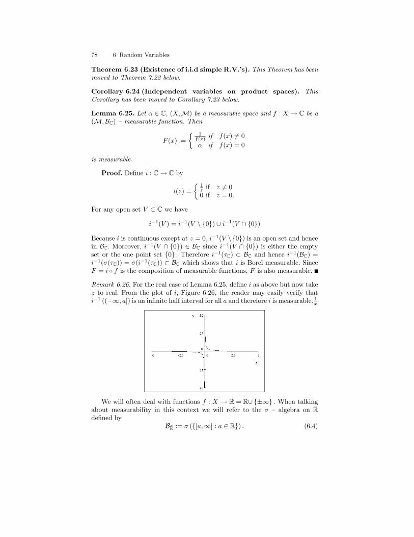
78 6 Random Variables
Theorem 6.23 (Existence of i.i.d simple R.V.’s). This Theorem has beenmoved to Theorem 7.22 below.
Corollary 6.24 (Independent variables on product spaces). ThisCorollary has been moved to Corollary 7.23 below.
Lemma 6.25. Let α ∈ C, (X,M) be a measurable space and f : X → C be a(M,BC) – measurable function. Then
F (x) := 1
f(x) if f(x) 6= 0α if f(x) = 0
is measurable.
Proof. Define i : C → C by
i(z) =
1z if z 6= 00 if z = 0.
For any open set V ⊂ C we have
i−1(V ) = i−1(V \ 0) ∪ i−1(V ∩ 0)
Because i is continuous except at z = 0, i−1(V \0) is an open set and hencein BC. Moreover, i−1(V ∩ 0) ∈ BC since i−1(V ∩ 0) is either the emptyset or the one point set 0 . Therefore i−1(τC) ⊂ BC and hence i−1(BC) =i−1(σ(τC)) = σ(i−1(τC)) ⊂ BC which shows that i is Borel measurable. SinceF = i f is the composition of measurable functions, F is also measurable.
Remark 6.26. For the real case of Lemma 6.25, define i as above but now takez to real. From the plot of i, Figure 6.26, the reader may easily verify thati−1 ((−∞, a]) is an infinite half interval for all a and therefore i is measurable. 1
x
We will often deal with functions f : X → R = R∪±∞ . When talkingabout measurability in this context we will refer to the σ – algebra on Rdefined by
BR := σ ([a,∞] : a ∈ R) . (6.4)
6.1 Measurable Functions 79
Proposition 6.27 (The Structure of BR). Let BR and BR be as above, then
BR = A ⊂ R : A ∩ R ∈BR. (6.5)
In particular ∞ , −∞ ∈ BR and BR ⊂ BR.
Proof. Let us first observe that
−∞ = ∩∞n=1[−∞,−n) = ∩∞n=1[−n,∞]c ∈ BR,
∞ = ∩∞n=1[n,∞] ∈ BR and R = R\ ±∞ ∈ BR.
Letting i : R → R be the inclusion map,
i−1 (BR) = σ(i−1
([a,∞] : a ∈ R
))= σ
(i−1 ([a,∞]) : a ∈ R
)= σ
([a,∞] ∩ R : a ∈ R
)= σ ([a,∞) : a ∈ R) = BR.
Thus we have shown
BR = i−1 (BR) = A ∩ R : A ∈ BR.
This implies:
1. A ∈ BR =⇒ A ∩ R ∈BR and2. if A ⊂ R is such that A ∩ R ∈BR there exists B ∈ BR such that A ∩ R =B ∩ R. Because A∆B ⊂ ±∞ and ∞ , −∞ ∈ BR we may concludethat A ∈ BR as well.
This proves Eq. (6.5).The proofs of the next two corollaries are left to the reader, see Exercises
6.5 and 6.6.
Corollary 6.28. Let (X,M) be a measurable space and f : X → R be afunction. Then the following are equivalent
1. f is (M,BR) - measurable,2. f−1((a,∞]) ∈M for all a ∈ R,3. f−1((−∞, a]) ∈M for all a ∈ R,4. f−1(−∞) ∈M, f−1(∞) ∈M and f0 : X → R defined by
f0 (x) := 1R (f (x)) =f (x) if f (x) ∈ R
0 if f (x) ∈ ±∞
is measurable.
Corollary 6.29. Let (X,M) be a measurable space, f, g : X → R be functionsand define f ·g : X → R and (f + g) : X → R using the conventions, 0 ·∞ = 0and (f + g) (x) = 0 if f (x) = ∞ and g (x) = −∞ or f (x) = −∞ andg (x) = ∞. Then f · g and f + g are measurable functions on X if both f andg are measurable.
80 6 Random Variables
Exercise 6.5. Prove Corollary 6.28 noting that the equivalence of items 1. –3. is a direct analogue of Corollary 6.7. Use Proposition 6.27 to handle item4.
Exercise 6.6. Prove Corollary 6.29.
Proposition 6.30 (Closure under sups, infs and limits). Suppose that(X,M) is a measurable space and fj : (X,M) → R for j ∈ N is a sequenceof M/BR – measurable functions. Then
supjfj , infjfj , lim supj→∞
fj and lim infj→∞
fj
are all M/BR – measurable functions. (Note that this result is in generallyfalse when (X,M) is a topological space and measurable is replaced by con-tinuous in the statement.)
Proof. Define g+(x) := sup jfj(x), then
x : g+(x) ≤ a = x : fj(x) ≤ a ∀ j= ∩jx : fj(x) ≤ a ∈ M
so that g+ is measurable. Similarly if g−(x) = infj fj(x) then
x : g−(x) ≥ a = ∩jx : fj(x) ≥ a ∈ M.
Since
lim supj→∞
fj = infn
sup fj : j ≥ n and
lim infj→∞
fj = supn
inf fj : j ≥ n
we are done by what we have already proved.
Definition 6.31. Given a function f : X → R let f+(x) := max f(x), 0and f− (x) := max (−f(x), 0) = −min (f(x), 0) . Notice that f = f+ − f−.
Corollary 6.32. Suppose (X,M) is a measurable space and f : X → R is afunction. Then f is measurable iff f± are measurable.
Proof. If f is measurable, then Proposition 6.30 implies f± are measur-able. Conversely if f± are measurable then so is f = f+ − f−.
Definition 6.33. Let (X,M) be a measurable space. A function ϕ : X → F(F denotes either R, C or [0,∞] ⊂ R) is a simple function if ϕ is M – BFmeasurable and ϕ(X) contains only finitely many elements.

6.1 Measurable Functions 81
Any such simple functions can be written as
ϕ =n∑
i=1
λi1Aiwith Ai ∈M and λi ∈ F. (6.6)
Indeed, take λ1, λ2, . . . , λn to be an enumeration of the range of ϕ and Ai =ϕ−1(λi). Note that this argument shows that any simple function may bewritten intrinsically as
ϕ =∑y∈F
y1ϕ−1(y). (6.7)
The next theorem shows that simple functions are “pointwise dense” inthe space of measurable functions.
Theorem 6.34 (Approximation Theorem). Let f : X → [0,∞] be mea-surable and define, see Figure 6.4,
ϕn(x) :=n2n−1∑
k=0
k
2n1f−1(( k
2n , k+12n ])(x) + n1f−1((n2n,∞])(x)
=n2n−1∑
k=0
k
2n1 k
2n <f≤ k+12n (x) + n1f>n2n(x)
then ϕn ≤ f for all n, ϕn(x) ↑ f(x) for all x ∈ X and ϕn ↑ f uniformly onthe sets XM := x ∈ X : f(x) ≤M with M <∞.
Moreover, if f : X → C is a measurable function, then there exists simplefunctions ϕn such that limn→∞ ϕn(x) = f(x) for all x and |ϕn| ↑ |f | asn→∞.
Proof. Since
(k
2n,k + 12n
] = (2k
2n+1,2k + 12n+1
] ∪ (2k + 12n+1
,2k + 22n+1
],
if x ∈ f−1(( 2k2n+1 ,
2k+12n+1 ]
)then ϕn(x) = ϕn+1(x) = 2k
2n+1 and if x ∈f−1
(( 2k+1
2n+1 ,2k+22n+1 ]
)then ϕn(x) = 2k
2n+1 <2k+12n+1 = ϕn+1(x). Similarly
(2n,∞] = (2n, 2n+1] ∪ (2n+1,∞],
and so for x ∈ f−1((2n+1,∞]), ϕn(x) = 2n < 2n+1 = ϕn+1(x) and forx ∈ f−1((2n, 2n+1]), ϕn+1(x) ≥ 2n = ϕn(x). Therefore ϕn ≤ ϕn+1 for alln. It is clear by construction that ϕn(x) ≤ f(x) for all x and that 0 ≤f(x) − ϕn(x) ≤ 2−n if x ∈ X2n . Hence we have shown that ϕn(x) ↑ f(x) forall x ∈ X and ϕn ↑ f uniformly on bounded sets. For the second assertion,first assume that f : X → R is a measurable function and choose ϕ±n to besimple functions such that ϕ±n ↑ f± as n → ∞ and define ϕn = ϕ+
n − ϕ−n .Then

82 6 Random Variables
Fig. 6.4. Constructing simple functions approximating a function, f : X → [0,∞].
|ϕn| = ϕ+n + ϕ−n ≤ ϕ+
n+1 + ϕ−n+1 = |ϕn+1|
and clearly |ϕn| = ϕ+n +ϕ−n ↑ f++f− = |f | and ϕn = ϕ+
n −ϕ−n → f+−f− = fas n→∞. Now suppose that f : X → C is measurable. We may now choosesimple function un and vn such that |un| ↑ |Re f | , |vn| ↑ |Im f | , un → Re fand vn → Im f as n→∞. Let ϕn = un + ivn, then
|ϕn|2 = u2n + v2
n ↑ |Re f |2 + |Im f |2 = |f |2
and ϕn = un + ivn → Re f + i Im f = f as n→∞.
6.2 Factoring Random Variables
Lemma 6.35. Suppose that (Y,F) is a measurable space and F : X → Y isa map. Then to every (σ(F ),BR) – measurable function, H : X → R, there isa (F ,BR) – measurable function h : Y → R such that H = h F.
Proof. First suppose that H = 1A where A ∈ σ(F ) = F−1(F). LetB ∈ F such that A = F−1(B) then 1A = 1F−1(B) = 1B F and hence theLemma is valid in this case with h = 1B . More generally if H =
∑ai1Ai
is a simple function, then there exists Bi ∈ F such that 1Ai= 1Bi
F andhence H = h F with h :=
∑ai1Bi
– a simple function on R. For general(σ(F ),F) – measurable function, H, from X → R, choose simple functionsHn converging to H. Let hn be simple functions on R such that Hn = hn F.Then it follows that
H = limn→∞
Hn = lim supn→∞
Hn = lim supn→∞
hn F = h F

6.2 Factoring Random Variables 83
where h := lim supn→∞
hn – a measurable function from Y to R.
The following is an immediate corollary of Proposition 6.16 and Lemma6.35.
Corollary 6.36. Let X and A be sets, and suppose for α ∈ A we are give ameasurable space (Yα,Fα) and a function fα : X → Yα. Let Y :=
∏α∈A Yα,
F := ⊗α∈AFα be the product σ – algebra on Y and M := σ(fα : α ∈ A)be the smallest σ – algebra on X such that each fα is measurable. Then thefunction F : X → Y defined by [F (x)]α := fα(x) for each α ∈ A is (M,F)– measurable and a function H : X → R is (M,BR) – measurable iff thereexists a (F ,BR) – measurable function h from Y to R such that H = h F.

7
Independence
7.1 π – λ and Monotone Class Theorems
Definition 7.1. Let C ⊂ 2X be a collection of sets.
1. C is a monotone class if it is closed under countable increasing unionsand countable decreasing intersections,
2. C is a π – class if it is closed under finite intersections and3. C is a λ–class if C satisfies the following properties:
a) X ∈ Cb) If A,B ∈ C and A ⊂ B, then B \ A ∈ C. (Closed under proper
differences.)c) If An ∈ C and An ↑ A, then A ∈ C. (Closed under countable increasing
unions.)
Remark 7.2. If C is a collection of subsets of Ω which is both a λ – class anda π – system then C is a σ – algebra. Indeed, since Ac = X \ A, we see thatany λ - system is closed under complementation. If C is also a π – system,it is closed under intersections and therefore C is an algebra. Since C is alsoclosed under increasing unions, C is a σ – algebra.
Lemma 7.3 (Alternate Axioms for a λ – System*). Suppose that L ⊂2Ω is a collection of subsets Ω. Then L is a λ – class iff λ satisfies the followingpostulates:
1. X ∈ L2. A ∈ L implies Ac ∈ L. (Closed under complementation.)3. If An∞n=1 ⊂ L are disjoint, the
∑∞n=1An ∈ L. (Closed under disjoint
unions.)
Proof. Suppose that L satisfies a. – c. above. Clearly then postulates 1.and 2. hold. Suppose that A,B ∈ L such that A ∩B = ∅, then A ⊂ Bc and
Ac ∩Bc = Bc \A ∈ L.
Taking compliments of this result shows A ∪B ∈ L as well. So by induction,Bm :=
∑mn=1An ∈ L. Since Bm ↑
∑∞n=1An it follows from postulate c. that∑∞
n=1An ∈ L.Now suppose that L satisfies postulates 1. – 3. above. Notice that ∅ ∈ L and
by postulate 3., L is closed under finite disjoint unions. Therefore if A,B ∈ L

86 7 Independence
with A ⊂ B, then Bc ∈ L and A ∩ Bc = ∅ allows us to conclude thatA ∪Bc ∈ L. Taking complements of this result shows B \A = Ac ∩B ∈ L aswell, i.e. postulate b. holds. If An ∈ L with An ↑ A, then Bn := An \An−1 ∈ Lfor all n, where by convention A0 = ∅. Hence it follows by postulate 3 that∪∞n=1An =
∑∞n=1Bn ∈ L.
Theorem 7.4 (Dynkin’s π – λ Theorem). If L is a λ class which containsa contains a π – class, P, then σ(P) ⊂ L.
Proof. We start by proving the following assertion; for any element C ∈ L,the collection of sets,
LC := D ∈ L : C ∩D ∈ L ,
is a λ – system. To prove this claim, observe that: a. X ∈ LC , b. if A ⊂ Bwith A,B ∈ LC , then A ∩ C, B ∩ C ∈ L with A ∩ C ⊂ B \ C and
(B \A) ∩ C = [B ∩ C] \A = [B ∩ C] \ [A ∩ C] ∈ L.
Therefore LC is closed under proper differences. Finally, c. if An ∈ LC withAn ↑ A, then An ∩ C ∈ L and An ∩ C ↑ A ∩ C ∈ L, i.e. A ∈ LC . Hence wehave verified LC is still a λ – system.
For the rest of the proof, we may assume with out loss of generality that Lis the smallest λ – class containing P – if not just replace L by the intersectionof all λ – classes containing P. Then for C ∈ P we know that LC ⊂ L is aλ - class containing P and hence LC = L. Since C ∈ P was arbitrary, wehave shown, C ∩ D ∈ L for all C ∈ P and D ∈ L. We may now concludethat if C ∈ L, then P ⊂ LC ⊂ L and hence again LC = L. Since C ∈ L isarbitrary, we have shown C ∩D ∈ L for all C,D ∈ L, i.e. L is a π – system.So by Remark 7.2, L is a σ algebra. Since σ (P) is the smallest σ – algebracontaining P it follows that σ (P) ⊂ L.
As an immediate corollary, we have the following uniqueness result.
Proposition 7.5. Suppose that P ⊂ 2Ω is a π – system. If P and Q are twoprobability1 measures on σ (P) such that P = Q on P, then P = Q on σ (P) .
Proof. Let L := A ∈ σ (P) : P (A) = Q (A) . One easily shows L is a λ– class which contains P by assumption. Indeed, Ω ∈ P ⊂ L, if A,B ∈ L withA ⊂ B, then
P (B \A) = P (B)− P (A) = Q (B)−Q (A) = Q (B \A)
so that B\A ∈ L, and if An ∈ L with An ↑ A, then P (A) = limn→∞ P (An) =limn→∞Q (An) = Q (A) which shows A ∈ L. Therefore σ (P) ⊂ L = σ (P)and the proof is complete.1 More generally, P and Q could be two measures such that P (Ω) = Q (Ω) < ∞.

7.1 π – λ and Monotone Class Theorems 87
Example 7.6. Let Ω := a, b, c, d and let µ and ν be the probability measureon 2Ω determined by, µ (x) = 1
4 for all x ∈ Ω and ν (a) = ν (d) = 18
and ν (b) = ν (c) = 3/8. In this example,
L :=A ∈ 2Ω : P (A) = Q (A)
is λ – system which is not an algebra. Indeed, A = a, b and B = a, c arein L but A ∩B /∈ L.
Exercise 7.1. Suppose that µ and ν are two measure on a measure space,(Ω,B) such that µ = ν on a π – system, P. Further assume B = σ (P) andthere exists Ωn ∈ P such that; i) µ (Ωn) = ν (Ωn) < ∞ for all n and ii)Ωn ↑ Ω as n ↑ ∞. Show µ = ν on B.
Hint: Consider the measures, µn (A) := µ (A ∩Ωn) and νn (A) =ν (A ∩Ωn) .
Solution to Exercise (7.1). Let µn (A) := µ (A ∩Ωn) and νn (A) =ν (A ∩Ωn) for all A ∈ B. Then µn and νn are finite measure such µn (Ω) =νn (Ω) and µn = νn on P. Therefore by Proposition 7.5, µn = νn on B. So bythe continuity properties of µ and ν, it follows that
µ (A) = limn→∞
µ (A ∩Ωn) = limn→∞
µn (A) = limn→∞
νn (A) = limn→∞
ν (A ∩Ωn) = ν (A)
for all A ∈ B.
Corollary 7.7. A probability measure, P, on (R,BR) is uniquely determinedby its distribution function,
F (x) := P ((−∞, x]) .
Definition 7.8. Suppose that Xini=1 is a sequence of random variables on
a probability space, (Ω,B, P ) . The measure, µ = P (X1, . . . , Xn)−1 on BRn
is called the joint distribution of (X1, . . . , Xn) . To be more explicit,
µ (B) := P ((X1, . . . , Xn) ∈ B) := P (ω ∈ Ω : (X1 (ω) , . . . , Xn (ω)) ∈ B)
for all B ∈ BRn .
Corollary 7.9. The joint distribution, µ is uniquely determined from theknowledge of
P ((X1, . . . , Xn) ∈ A1 × · · · ×An) for all Ai ∈ BR
or from the knowledge of
P (X1 ≤ x1, . . . , Xn ≤ xn) for all Ai ∈ BR
for all x = (x1, . . . , xn) ∈ Rn.

88 7 Independence
Proof. Apply Proposition 7.5 with P being the π – systems defined by
P := A1 × · · · ×An ∈ BRn : Ai ∈ BR
for the first case and
P := (−∞, x1]× · · · × (−∞, xn] ∈ BRn : xi ∈ R
for the second case.
Definition 7.10. Suppose that Xini=1 and Yin
i=1 are two finite sequencesof random variables on two probability spaces, (Ω,B, P ) and (X,F , Q) respec-tively. We write (X1, . . . , Xn) d= (Y1, . . . , Yn) if (X1, . . . , Xn) and (Y1, . . . , Yn)have the same distribution, i.e. if
P ((X1, . . . , Xn) ∈ B) = Q ((Y1, . . . , Yn) ∈ B) for all B ∈ BRn .
More generally, if Xi∞i=1 and Yi∞i=1 are two sequences of random variables
on two probability spaces, (Ω,B, P ) and (X,F , Q) we write Xi∞i=1d= Yi∞i=1
iff (X1, . . . , Xn) d= (Y1, . . . , Yn) for all n ∈ N.
Exercise 7.2. Let Xi∞i=1 and Yi∞i=1 be two sequences of random variables
such that Xi∞i=1d= Yi∞i=1 . Let Sn∞n=1 and Tn∞n=1 be defined by, Sn :=
X1 + · · ·+Xn and Tn := Y1 + · · ·+ Yn. Prove the following assertions.
1. Suppose that f : Rn → Rk is a BRn/BRk – measurable function, thenf (X1, . . . , Xn) d= f (Y1, . . . , Yn) .
2. Use your result in item 1. to show Sn∞n=1d= Tn∞n=1 .
Hint: apply item 1. with k = n and a judiciously chosen function, f :Rn → Rn.
3. Show lim supn→∞
Xnd= lim sup
n→∞Yn and similarly that lim infn→∞Xn
d=
lim infn→∞ Yn.Hint: with the aid of the set identity,
lim supn→∞
Xn ≥ x
= Xn ≥ x i.o. ,
show
P
(lim sup
n→∞Xn ≥ x
)= lim
n→∞lim
m→∞P (∪m
k=n Xk ≥ x) .
To use this identity you will also need to find B ∈ BRm such that
∪mk=n Xk ≥ x = (X1, . . . , Xm) ∈ B .

7.1 π – λ and Monotone Class Theorems 89
7.1.1 The Monotone Class Theorem
This subsection may be safely skipped!
Lemma 7.11 (Monotone Class Theorem*). Suppose A ⊂ 2X is an alge-bra and C is the smallest monotone class containing A. Then C = σ(A).
Proof. For C ∈ C let
C(C) = B ∈ C : C ∩B,C ∩Bc, B ∩ Cc ∈ C,
then C(C) is a monotone class. Indeed, if Bn ∈ C(C) and Bn ↑ B, thenBc
n ↓ Bc and so
C 3 C ∩Bn ↑ C ∩BC 3 C ∩Bc
n ↓ C ∩Bc andC 3 Bn ∩ Cc ↑ B ∩ Cc.
Since C is a monotone class, it follows that C ∩ B,C ∩ Bc, B ∩ Cc ∈ C,i.e. B ∈ C(C). This shows that C(C) is closed under increasing limits anda similar argument shows that C(C) is closed under decreasing limits. Thuswe have shown that C(C) is a monotone class for all C ∈ C. If A ∈ A ⊂ C,then A ∩ B,A ∩ Bc, B ∩ Ac ∈ A ⊂ C for all B ∈ A and hence it followsthat A ⊂ C(A) ⊂ C. Since C is the smallest monotone class containing A andC(A) is a monotone class containing A, we conclude that C(A) = C for anyA ∈ A. Let B ∈ C and notice that A ∈ C(B) happens iff B ∈ C(A). Thisobservation and the fact that C(A) = C for all A ∈ A implies A ⊂ C(B) ⊂ Cfor all B ∈ C. Again since C is the smallest monotone class containing A andC(B) is a monotone class we conclude that C(B) = C for all B ∈ C. That isto say, if A,B ∈ C then A ∈ C = C(B) and hence A ∩B, A ∩Bc, Ac ∩B ∈ C.So C is closed under complements (since X ∈ A ⊂ C) and finite intersectionsand increasing unions from which it easily follows that C is a σ – algebra.
Exercise 7.3. Suppose that A ⊂ 2Ω is an algebra, B := σ (A) , and P isa probability measure on B. Show, using the π – λ theorem, that for everyB ∈ B there exists A ∈ A such that that P (A4B) < ε. Here
A4B := (A \B) ∪ (B \A)
is the symmetric difference of A and B.Hints:
1. It may be useful to observe that
1A4B = |1A − 1B |
so that P (A4B) = E |1A − 1B | .

90 7 Independence
2. Also observe that if B = ∪Bi and A = ∪iAi, then
B \A ⊂ ∪i (Bi \Ai) ⊂ ∪iAi 4Bi andA \B ⊂ ∪i (Ai \Bi) ⊂ ∪iAi 4Bi
so thatA4B ⊂ ∪i (Ai 4Bi) .
3. We also have
(B2 \B1) \ (A2 \A1) = B2 ∩Bc1 ∩ (A2 \A1)
c
= B2 ∩Bc1 ∩ (A2 ∩Ac
1)c
= B2 ∩Bc1 ∩ (Ac
2 ∪A1)= [B2 ∩Bc
1 ∩Ac2] ∪ [B2 ∩Bc
1 ∩A1]⊂ (B2 \A2) ∪ (A1 \B1)
and similarly,
(A2 \A1) \ (B2 \B1) ⊂ (A2 \B2) ∪ (B1 \A1)
so that
(A2 \A1)4 (B2 \B1) ⊂ (B2 \A2) ∪ (A1 \B1) ∪ (A2 \B2) ∪ (B1 \A1)= (A1 4B1) ∪ (A2 4B2) .
4. Observe that An ∈ B and An ↑ A, then
P (B 4An) = P (B \An)+P (An \B) → P (B \A)+P (A \B) = P (A4B) .
5. Let L be the collection of sets B for which the assertion of the theoremholds. Show L is a λ – system which contains A.
Solution to Exercise (7.3). Since L contains the π – system, A it sufficesby the π – λ theorem to show L is a λ – system. Clearly, Ω ∈ L sinceΩ ∈ A ⊂ L. If B1 ⊂ B2 with Bi ∈ L and ε > 0, there exists Ai ∈ A such thatP (Bi 4Ai) = E |1Ai − 1Bi | < ε/2 and therefore,
P ((B2 \B1)4 (A2 \A1)) ≤ P ((A1 4B1) ∪ (A2 4B2))≤ P ((A1 4B1)) + P ((A2 4B2)) < ε.
Also if Bn ↑ B with Bn ∈ L, there exists An ∈ A such that P (Bn 4An) <ε2−n and therefore,
P ([∪nBn]4 [∪nAn]) ≤∞∑
n=1
P (Bn 4An) < ε.
Moreover, if we let B := ∪nBn and AN := ∪Nn=1An, then
P(B 4AN
)= P
(B \AN
)+P
(AN \B
)→ P (B \A)+P (A \B) = P (B 4A)
where A := ∪nAn. Hence it follows for N large enough that P(B 4AN
)< ε.

7.2 Basic Properties of Independence 91
7.2 Basic Properties of Independence
For this section we will suppose that (Ω,B, P ) is a probability space.
Definition 7.12. We say that A is independent of B is P (A|B) = P (A) orequivalently that
P (A ∩B) = P (A)P (B) .
We further say a finite sequence of collection of sets, Cini=1 , are independent
ifP (∩j∈JAj) =
∏j∈J
P (Aj)
for all Ai ∈ Ci and J ⊂ 1, 2, . . . , n .
Observe that if Cini=1 , are independent classes then so are Ci ∪ Xn
i=1 .Moreover, if we assume that X ∈ Ci for each i, then Cin
i=1 , are independentiff
P(∩n
j=1Aj
)=
n∏j=1
P (Aj) for all (A1, . . . , An) ∈ C1 × · · · × Cn.
Theorem 7.13. Suppose that Cini=1 is a finite sequence of independent π –
classes. Then σ (Ci)ni=1 are also independent.
Proof. As mentioned above, we may always assume with out loss of gen-erality that X ∈ Ci. Fix, Aj ∈ Cj for j = 2, 3, . . . , n. We will begin by showingthat
P (A ∩A2 ∩ · · · ∩An) = P (A)P (A2) . . . P (An) for all A ∈ σ (C1) . (7.1)
Since it is clear that this identity holds if P (Aj) = 0 for some j = 2, . . . , n,we may assume that P (Aj) > 0 for j ≥ 2. In this case we may define,
Q (A) =P (A ∩A2 ∩ · · · ∩An)P (A2) . . . P (An)
=P (A ∩A2 ∩ · · · ∩An)P (A2 ∩ · · · ∩An)
= P (A|A2 ∩ · · · ∩An) for all A ∈ σ (C1) .
Then equation Eq. (7.1) is equivalent to P (A) = Q (A) on σ (C1) . But this istrue by Proposition 7.5 using the fact that Q = P on the π – system, C1.
Since (A2, . . . , An) ∈ C2 × · · · × Cn were arbitrary we may now concludethat σ (C1) , C2, . . . , Cn are independent.
By applying the result we have just proved to the sequence, C2, . . . , Cn, σ (C1)shows that σ (C2) , C3, . . . , Cn, σ (C1) are independent. Similarly we show induc-tively that
σ (Cj) , Cj+1, . . . , Cn, σ (C1) , . . . , σ (Cj−1)
are independent for each j = 1, 2, . . . , n. The desired result occurs at j = n.
92 7 Independence
Definition 7.14. A collection of subsets of B, Ctt∈T is said to be indepen-dent iff Ctt∈Λ are independent for all finite subsets, Λ ⊂ T. More explicitly,we are requiring
P (∩t∈ΛAt) =∏t∈Λ
P (At)
whenever Λ is a finite subset of T and At ∈ Ct for all t ∈ Λ.
Corollary 7.15. If Ctt∈T is a collection of independent classes such thateach Ct is a π – system, then σ (Ct)t∈T are independent as well.
Example 7.16. Suppose that Ω = Λn where Λ is a finite set, B = 2Ω ,P (ω) =
∏nj=1 qj (ωj) where qj : Λ → [0, 1] are functions such that∑
λ∈Λ qj (λ) = 1. Let Ci :=Λi−1 ×A× Λn−i : A ⊂ Λ
. Then Cin
i=1 areindependent. Indeed, if Bi := Λi−1 ×Ai × Λn−i, then
∩Bi = A1 ×A2 × · · · ×An
and we have
P (∩Bi) =∑
ω∈A1×A2×···×An
n∏i=1
qi (ωi) =n∏
i=1
∑λ∈Ai
qi (λ)
while
P (Bi) =∑
ω∈Λi−1×Ai×Λn−i
n∏i=1
qi (ωi) =∑
λ∈Ai
qi (λ) .
Definition 7.17. A collections of random variables, Xt : t ∈ T are inde-pendent iff σ (Xt) : t ∈ T are independent.
Theorem 7.18. Let X := Xt : t ∈ T be a collection of random variables.Then the following are equivalent:
1. The collection X,2.
P (∩t∈Λ Xt ∈ At) =∏t∈Λ
P (Xt ∈ At)
for all finite subsets, Λ ⊂ T, and all At ∈ BR for t ∈ Λ.3.
P (∩t∈Λ Xt ≤ xt) =∏t∈Λ
P (Xt ≤ xt)
for all finite subsets, Λ ⊂ T, and all xt ∈ R for t ∈ Λ.
Proof. The equivalence of 1. and 2. follows almost immediately form thedefinition of independence and the fact that σ (Xt) = Xt ∈ A : A ∈ BR .Clearly 2. implies 3. holds. Finally, 3. implies 2. is an application of Corollary7.15 with Ct := Xt ≤ a : a ∈ R and making use the observations that Ct
is a π – system for all t and that σ (Ct) = σ (Xt) .
7.2 Basic Properties of Independence 93
Example 7.19. Continue the notation of Example 7.16 and further assume thatΛ ⊂ R and let Xi : Ω → Λ be defined by, Xi (ω) = ωi. Then Xin
i=1 areindependent random variables. Indeed, σ (Xi) = Ci with Ci as in Example7.16.
Alternatively, from Exercise 4.1, we know that
EP
[n∏
i=1
fi (Xi)
]=
n∏i=1
EP [fi (Xi)]
for all fi : Λ → R. Taking Ai ⊂ Λ and fi := 1Ai in the above identity showsthat
P (X1 ∈ A1, . . . , Xn ∈ An) = EP
[n∏
i=1
1Ai (Xi)
]=
n∏i=1
EP [1Ai (Xi)]
=n∏
i=1
P (Xi ∈ Ai)
as desired.
Corollary 7.20. A sequence of random variables, Xjkj=1 with countable
ranges are independent iff
P(∩k
j=1 Xj = xj)
=k∏
j=1
P (Xj = xj) (7.2)
for all xj ∈ R.
Proof. Observe that both sides of Eq. (7.2) are zero unless xj is in therange of Xj for all j. Hence it suffices to verify Eq. (7.2) for those xj ∈Ran(Xj) =: Rj for all j. Now if Xjk
j=1 are independent, then Xj = xj ∈σ (Xj) for all xj ∈ R and therefore Eq. (7.2) holds.
Conversely if Eq. (7.2) and Vj ∈ BR, then

94 7 Independence
P(∩k
j=1 Xj ∈ Vj)
= P
∩kj=1
∑xj∈Vj∩Rj
Xj = xj
= P
∑(x1,...,xk)∈
Qkj=1 Vj∩Rj
[∩k
j=1 Xj = xj]
=∑
(x1,...,xk)∈Qk
j=1 Vj∩Rj
P([∩k
j=1 Xj = xj])
=∑
(x1,...,xk)∈Qk
j=1 Vj∩Rj
k∏j=1
P (Xj = xj)
=k∏
j=1
∑xj∈Vj∩Rj
P (Xj = xj) =k∏
j=1
P (Xj ∈ Vj) .
Definition 7.21. As sequences of random variables, Xn∞n=1 , on a proba-bility space, (Ω,B, P ), are i.i.d. (= independent and identically dis-tributed) if they are independent and (Xn)∗ P = (Xk)∗ P for all k, n. Thatis we should have
P (Xn ∈ A) = P (Xk ∈ A) for all k, n ∈ N and A ∈ BR.
Observe that Xn∞n=1 are i.i.d. random variables iff
P (X1 ∈ A1, . . . , Xn ∈ An) =n∏
j=1
P (Xi ∈ Ai) =n∏
j=1
P (X1 ∈ Ai) =n∏
j=1
µ (Ai)
(7.3)where µ = (X1)∗ P. The identity in Eq. (7.3) is to hold for all n ∈ N and allAi ∈ BR.
Theorem 7.22 (Existence of i.i.d simple R.V.’s). Suppose that qini=0
is a sequence of positive numbers such that∑n
i=0 qi = 1. Then there ex-ists a sequence Xk∞k=1 of simple random variables taking values in Λ =0, 1, 2 . . . , n on ((0, 1],B,m) such that
m (X1 = i1, . . . , Xk = ii) = qi1 . . . qik
for all i1, i2, . . . , ik ∈ 0, 1, 2, . . . , n and all k ∈ N.
Proof. For i = 0, 1, . . . , n, let σ−1 = 0 and σj :=∑j
i=0 qi and for anyinterval, (a, b], let
Ti ((a, b]) := (a+ σi−1 (b− a) , a+ σi (b− a)].
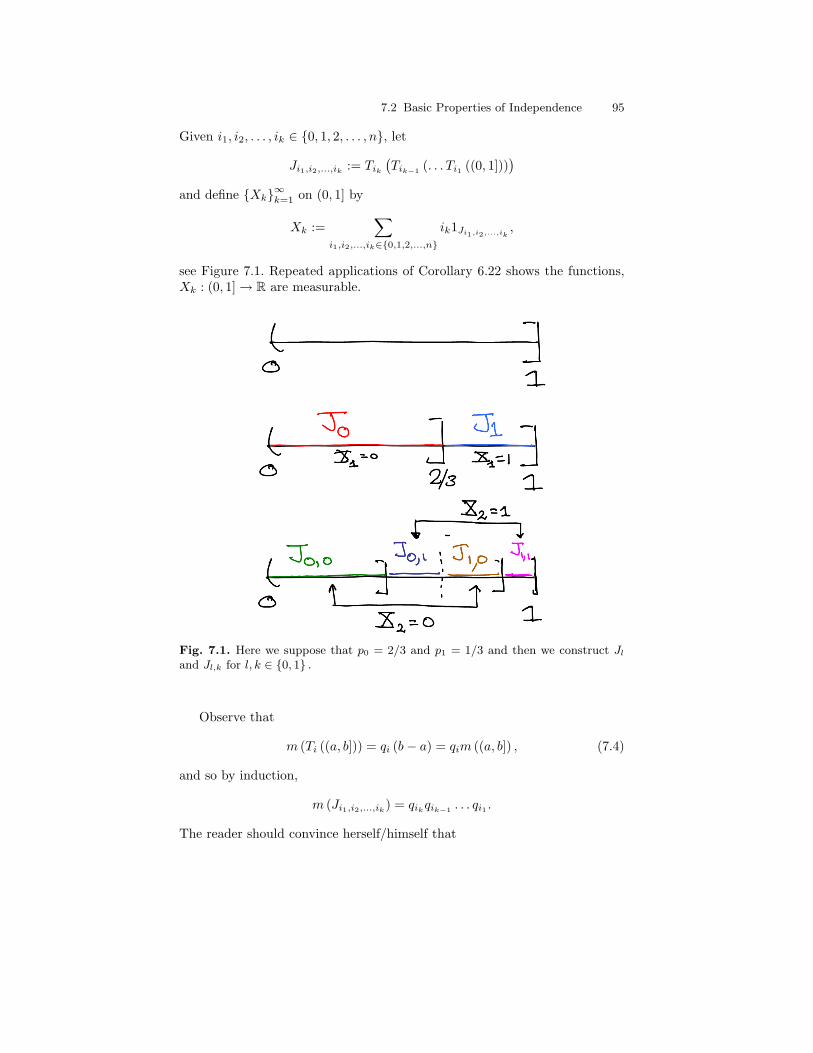
7.2 Basic Properties of Independence 95
Given i1, i2, . . . , ik ∈ 0, 1, 2, . . . , n, let
Ji1,i2,...,ik:= Tik
(Tik−1 (. . . Ti1 ((0, 1]))
)and define Xk∞k=1 on (0, 1] by
Xk :=∑
i1,i2,...,ik∈0,1,2,...,n
ik1Ji1,i2,...,ik,
see Figure 7.1. Repeated applications of Corollary 6.22 shows the functions,Xk : (0, 1] → R are measurable.
Fig. 7.1. Here we suppose that p0 = 2/3 and p1 = 1/3 and then we construct Jl
and Jl,k for l, k ∈ 0, 1 .
Observe that
m (Ti ((a, b])) = qi (b− a) = qim ((a, b]) , (7.4)
and so by induction,
m (Ji1,i2,...,ik) = qik
qik−1 . . . qi1 .
The reader should convince herself/himself that

96 7 Independence
X1 = i1, . . . Xk = ii = Ji1,i2,...,ik
and therefore, we have
m (X1 = i1, . . . , Xk = ii) = m (Ji1,i2,...,ik) = qik
qik−1 . . . qi1
as desired.
Corollary 7.23 (Independent variables on product spaces). SupposeΛ = 0, 1, 2 . . . , n , qi > 0 with
∑ni=0 qi = 1, Ω = Λ∞ = ΛN, and for i ∈
N, let Yi : Ω → R be defined by Yi (ω) = ωi for all ω ∈ Ω. Further letB := σ (Y1, Y2, . . . , Yn, . . . ) . Then there exists a unique probability measure,P : B → [0, 1] such that
P (Y1 = i1, . . . , Yk = ii) = qi1 . . . qik.
Proof. Let Xini=1 be as in Theorem 7.22 and define T : (0, 1] → Ω by
T (x) = (X1 (x) , X2 (x) , . . . , Xk (x) , . . . ) .
Observe that T is measurable since Yi T = Xi is measurable for all i. Wenow define, P := T∗m. Then we have
P (Y1 = i1, . . . , Yk = ii) = m(T−1 (Y1 = i1, . . . , Yk = ii)
)= m (Y1 T = i1, . . . , Yk T = ii)= m (X1 = i1, . . . , Xk = ii) = qi1 . . . qik
.
Theorem 7.24. Given a finite subset, Λ ⊂ R and a function q : Λ → [0, 1]such that
∑λ∈Λ q (λ) = 1, there exists a probability space, (Ω,B, P ) and an
independent sequence of random variables, Xn∞n=1 such that P (Xn = λ) =q (λ) for all λ ∈ Λ.
Proof. Use Corollary 7.20 to shows that random variables constructed inExample 5.28 or Theorem 7.22 fit the bill.
Proposition 7.25. Suppose that Xn∞n=1 is a sequence of i.i.d. randomvariables with distribution, P (Xn = 0) = P (Xn = 1) = 1
2 . If we let U :=∑∞n=1 2−nXn, then P (U ≤ x) = (0 ∨ x) ∧ 1, i.e. U has the uniform distribu-
tion on [0, 1] .
Proof. Let us recall that P (Xn = 0 a.a.) = P (Xn = 1 a.a.) . Hencewe may, by shrinking Ω if necessary, assume that Xn = 0 a.a. = ∅ =Xn = 1 a.a. . With this simplification, we have

7.2 Basic Properties of Independence 97U <
12
= X1 = 0 ,
U <14
= X1 = 0, X2 = 0 and
12≤ U <
34
= X1 = 1, X2 = 0
and hence that U <
34
=U <
12
∪
12≤ U <
34
= X1 = 0 ∪ X1 = 1, X2 = 0 .
From these identities, it follows that
P (U < 0) = 0, P(U <
14
)=
14, P
(U <
12
)=
12, and P
(U <
34
)=
34.
More generally, we claim that if x =∑n
j=1 εj2−j with εj ∈ 0, 1 , then
P (U < x) = x. (7.5)
The proof is by induction on n. Indeed, we have already verified (7.5) whenn = 1, 2. Suppose we have verified (7.5) up to some n ∈ N and let x =∑n
j=1 εj2−j and consider
P(U < x+ 2−(n+1)
)= P (U < x) + P
(x ≤ U < x+ 2−(n+1)
)= x+ P
(x ≤ U < x+ 2−(n+1)
).
Since x ≤ U < x+ 2−(n+1)
=[∩n
j=1 Xj = εj]∩ Xn+1 = 0
we see thatP(x ≤ U < x+ 2−(n+1)
)= 2−(n+1)
and henceP(U < x+ 2−(n+1)
)= x+ 2−(n+1)
which completes the induction argument.Since x → P (U < x) is left continuous we may now conclude that
P (U < x) = x for all x ∈ (0, 1) and since x → x is continuous we mayalso deduce that P (U ≤ x) = x for all x ∈ (0, 1) . Hence we may concludethat
P (U ≤ x) = (0 ∨ x) ∧ 1.

98 7 Independence
Lemma 7.26. Suppose that Bt : t ∈ T is an independent family of σ –fields. And further assume that T =
∑s∈S Ts and let
BTs= ∨t∈Ts
Bs = σ (∪t∈TsBs) .
Then BTss∈S is an independent family of σ fields.
Proof. Let
Cs = ∩α∈KBα : Bα ∈ Bα, K ⊂⊂ Ts .
It is now easily checked that Css∈S is an independent family of π – systems.Therefore BTs
= σ (Cs)s∈S is an independent family of σ – algebras.We may now show the existence of independent random variables with
arbitrary distributions.
Theorem 7.27. Suppose that µn∞n=1 are a sequence of probability measureson (R,BR) . Then there exists a probability space, (Ω,B, P ) and a sequenceYn∞n=1 independent random variables with Law (Yn) := P Y −1
n = µn forall n.
Proof. By Theorem 7.24, there exists a sequence of i.i.d. random variables,Zn∞n=1 , such that P (Zn = 1) = P (Zn = 0) = 1
2 . These random variablesmay be put into a two dimensional array, Xi,j : i, j ∈ N , see the proof of
Lemma 3.8. For each i, let Ui :=∑∞
j=1 2−iXi,j – σ(Xi,j∞j=1
)– measurable
random variable. According to Proposition 7.25, Ui is uniformly distributedon [0, 1] . Moreover by the grouping Lemma 7.26,
σ(Xi,j∞j=1
)∞i=1
are
independent σ – algebras and hence Ui∞i=1 is a sequence of i.i.d.. randomvariables with the uniform distribution.
Finally, let Fi (x) := µ ((−∞, x]) for all x ∈ R and let Gi (y) =inf x : Fi (x) ≥ y . Then according to Theorem 6.11, Yi := Gi (Ui) has µi asits distribution. Moreover each Yi is σ
(Xi,j∞j=1
)– measurable and therefore
the Yi∞i=1 are independent random variables.
7.2.1 An Example of Ranks
Let Xn∞n=1 be i.i.d. with common continuous distribution function, F. Inthis case we have, for any i 6= j, that
P (Xi = Xj) = µF ⊗ µF ((x, x) : x ∈ R) = 0.
This may be proved directly with some work or will be an easy consequenceof Fubini’s theorem to be considered later, see Example 10.11 below. For thedirect proof, let al∞l=−∞ be a sequence such that, al < al+1 for all l ∈ Z,liml→∞ al = ∞ and liml→−∞ al = −∞. Then

7.2 Basic Properties of Independence 99
(x, x) : x ∈ R ⊂ ∪l∈Z [(al, al+1]× (al, al+1]]
and therefore,
P (Xi = Xj) ≤∑l∈Z
P (Xi ∈ (al, al+1], Xj ∈ (al, al+1]) =∑l∈Z
[F (al+1)− F (al)]2
≤ supl∈Z
[F (al+1)− F (al)]∑l∈Z
[F (al+1)− F (al)] = supl∈Z
[F (al+1)− F (al)] .
Since F is continuous and F (∞+) = 1 and F (∞−) = 0, it is easily seen thatF is uniformly continuous on R. Therefore, if we choose al = l
N , we have
P (Xi = Xj) ≤ lim supN→∞
supl∈Z
[F
(l + 1N
)− F
(l
N
)]= 0.
Let Rn denote the “rank” of Xn in the list (X1, . . . , Xn) , i.e.
Rn :=n∑
j=1
1Xj>Xn = # j ≤ n : Xj > Xn .
For example if (X1, X2, X3, X4, X5, . . . ) = (9,−8, 3, 7, 23, . . . ) , we have R1 =1, R2 = 2, R3 = 2, and R4 = 2, R5 = 1. Observe that rank order, fromlowest to highest, of (X1, X2, X3, X4, X5) is (X2, X3, X4, X1, X5) . This canbe determined by the values of Ri for i = 1, 2, . . . , 5 as follows. Since R5 = 1,we must have X5 in the last slot, i.e. (∗, ∗, ∗, ∗, X5) . Since R4 = 2, we knowout of the remaining slots, X4 must be in the second from the far most right,i.e. (∗, ∗, X4, ∗, X5) . Since R3 = 2, we know that X3 is again the secondfrom the right of the remaining slots, i.e. we now know, (∗, X3, X4, ∗, X5) .Similarly, R2 = 2 implies (X2, X3, X4, ∗, X5) and finally R1 = 1 gives,(X2, X3, X4, X1, X5) . As another example, if Ri = i for i = 1, 2, . . . , n, thenXn < Xn−1 < · · · < X1.
Theorem 7.28 (Renyi Theorem). Let Xn∞n=1 be i.i.d. and assume thatF (x) := P (Xn ≤ x) is continuous. The Rn∞n=1 is an independent sequence,
P (Rn = k) =1n
for k = 1, 2, . . . , n,
and the events, An = Xn is a record = Rn = 1 are independent as nvaries and
P (An) = P (Rn = 1) =1n.
Proof. By Problem 6 on p. 110 of Resnick, (X1, . . . , Xn) and (Xσ1, . . . , Xσn)have the same distribution for any permutation σ.
Since F is continuous, it now follows that up to a set of measure zero,
Ω =∑
σ
Xσ1 < Xσ2 < · · · < Xσn
100 7 Independence
and therefore
1 = P (Ω) =∑
σ
P (Xσ1 < Xσ2 < · · · < Xσn) .
Since P (Xσ1 < Xσ2 < · · · < Xσn) is independent of σ we may now concludethat
P (Xσ1 < Xσ2 < · · · < Xσn) =1n!
for all σ. As observed before the statement of the theorem, to each realization(ε1, . . . , εn) , (here εi ∈ N with εi ≤ i) of (R1, . . . , Rn) there is a permutation,σ = σ (ε1, . . . , εn) such that Xσ1 < Xσ2 < · · · < Xσn. From this it followsthat
(R1, . . . , Rn) = (ε1, . . . , εn) = Xσ1 < Xσ2 < · · · < Xσn
and therefore,
P ((R1, . . . , Rn) = (ε1, . . . , εn)) = P (Xσ1 < Xσ2 < · · · < Xσn) =1n!.
Since
P (Rn = εn) =∑
(ε1,...εn−1)
P ((R1, . . . , Rn) = (ε1, . . . , εn))
=∑
(ε1,...εn−1)
1n!
= (n− 1)! · 1n!
=1n
we have shown that
P ((R1, . . . , Rn) = (ε1, . . . , εn)) =1n!
=n∏
j=1
1j
=n∏
j=1
P (Rj = εj) .
7.3 Borel-Cantelli Lemmas
Lemma 7.29 (First Borel Cantelli-Lemma). Suppose that An∞n=1 aremeasurable sets. If
∞∑n=1
P (An) <∞, (7.6)
thenP (An i.o.) = 0.

7.3 Borel-Cantelli Lemmas 101
Proof. First Proof. We have
P (An i.o.) = P (∩∞n=1 ∪k≥n Ak) = limn→∞
P (∪k≥nAk) ≤ limn→∞
∑k≥n
P (Ak) = 0.
(7.7)Second Proof. (Warning: this proof require integration theory which is
developed below.) Equation (7.6) is equivalent to
E
[ ∞∑n=1
1An
]<∞
from which it follows that∞∑
n=1
1An<∞ a.s.
which is equivalent to P (An i.o.) = 0.
Example 7.30. Suppose that Xn are Bernoulli random variables withP (Xn = 1) = pn and P (Xn = 0) = 1− pn. If∑
pn <∞
thenP (Xn = 1 i.o.) = 0
and henceP (Xn = 0 a.a.) = 1.
In particular,P(
limn→∞
Xn = 0)
= 1.
Figure 7.2 below serves as motivation for the following elementary lemmaon convex functions.
Lemma 7.31 (Convex Functions). Suppose that ϕ ∈ C2 ((a, b) → R) withϕ′′ (x) ≥ 0 for all x ∈ (a, b) . Then ϕ satisfies;
1. for all x0, x ∈ (a, b) ,
ϕ (x0) + ϕ′ (x0) (x− x0) ≤ ϕ (x)
and2. for all u ≤ v with u, v ∈ (a, b) ,
ϕ (u+ t (v − u)) ≤ ϕ (u) + t (ϕ (v)− ϕ (u)) ∀ t ∈ [0, 1] .
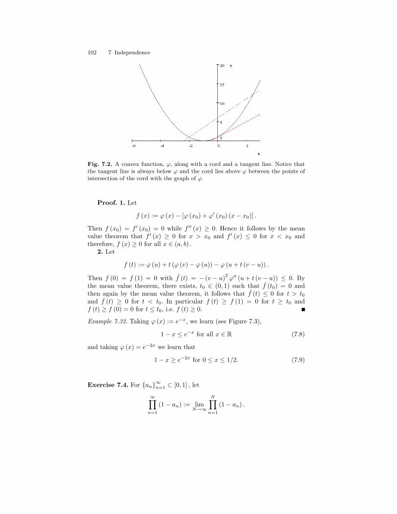
102 7 Independence
Fig. 7.2. A convex function, ϕ, along with a cord and a tangent line. Notice thatthe tangent line is always below ϕ and the cord lies above ϕ between the points ofintersection of the cord with the graph of ϕ.
Proof. 1. Let
f (x) := ϕ (x)− [ϕ (x0) + ϕ′ (x0) (x− x0)] .
Then f (x0) = f ′ (x0) = 0 while f ′′ (x) ≥ 0. Hence it follows by the meanvalue theorem that f ′ (x) ≥ 0 for x > x0 and f ′ (x) ≤ 0 for x < x0 andtherefore, f (x) ≥ 0 for all x ∈ (a, b) .
2. Let
f (t) := ϕ (u) + t (ϕ (v)− ϕ (u))− ϕ (u+ t (v − u)) .
Then f (0) = f (1) = 0 with f (t) = − (v − u)2 ϕ′′ (u+ t (v − u)) ≤ 0. Bythe mean value theorem, there exists, t0 ∈ (0, 1) such that f (t0) = 0 andthen again by the mean value theorem, it follows that f (t) ≤ 0 for t > t0and f (t) ≥ 0 for t < t0. In particular f (t) ≥ f (1) = 0 for t ≥ t0 andf (t) ≥ f (0) = 0 for t ≤ t0, i.e. f (t) ≥ 0.
Example 7.32. Taking ϕ (x) := e−x, we learn (see Figure 7.3),
1− x ≤ e−x for all x ∈ R (7.8)
and taking ϕ (x) = e−2x we learn that
1− x ≥ e−2x for 0 ≤ x ≤ 1/2. (7.9)
Exercise 7.4. For an∞n=1 ⊂ [0, 1] , let
∞∏n=1
(1− an) := limN→∞
N∏n=1
(1− an) .

7.3 Borel-Cantelli Lemmas 103
Fig. 7.3. A graph of 1− x and e−x showing that 1− x ≤ e−x for all x.
Fig. 7.4. A graph of 1− x and e−2x showing that 1− x ≥ e−2x for all x ∈ [0, 1/2] .
(The limit exists since,∏N
n=1 (1− an) ↓ as N ↑ .) Show that if an∞n=1 ⊂[0, 1), then
∞∏n=1
(1− an) = 0 iff∞∑
n=1
an = ∞.
Solution to Exercise (7.4). On one hand we have
N∏n=1
(1− an) ≤N∏
n=1
e−an = exp
(−
N∑n=1
an
)which upon passing to the limit as N →∞ gives
∞∏n=1
(1− an) ≤ exp
(−∞∑
n=1
an
).
Hence if∑∞
n=1 an = ∞ then∏∞
n=1 (1− an) = 0.
104 7 Independence
Conversely, suppose that∑∞
n=1 an < ∞. In this case an → 0 as n → ∞and so there exists an m ∈ N such that an ∈ [0, 1/2] for all n ≥ m. With thisnotation we then have for N ≥ m that
N∏n=1
(1− an) =m∏
n=1
(1− an) ·N∏
n=m+1
(1− an)
≥m∏
n=1
(1− an) ·N∏
n=m+1
e−2an =m∏
n=1
(1− an) · exp
(−2
N∑n=m+1
an
)
≥m∏
n=1
(1− an) · exp
(−2
∞∑n=m+1
an
).
So again letting N →∞ shows,
∞∏n=1
(1− an) ≥m∏
n=1
(1− an) · exp
(−2
∞∑n=m+1
an
)> 0.
Lemma 7.33 (Second Borel-Cantelli Lemma). Suppose that An∞n=1
are independent sets. If∞∑
n=1
P (An) = ∞, (7.10)
thenP (An i.o.) = 1. (7.11)
Combining this with the first Borel Cantelli Lemma gives the (Borel) Zero-Onelaw,
P (An i.o.) =
0 if∑∞
n=1 P (An) <∞1 if
∑∞n=1 P (An) = ∞ .
Proof. We are going to prove Eq. (7.11) by showing,
0 = P (An i.o.c) = P (Acn a.a) = P (∪∞n=1 ∩k≥n A
ck) .
Since ∩k≥nAck ↑ ∪∞n=1 ∩k≥n A
ck as n → ∞ and ∩m
k=nAck ↓ ∩∞n=1 ∪k≥n Ak as
m→∞,
P (∪∞n=1 ∩k≥n Ack) = lim
n→∞P (∩k≥nA
ck) = lim
n→∞lim
m→∞P (∩m≥k≥nA
ck) .
Making use of the independence of Ak∞k=1 and hence the independence ofAc
k∞k=1 , we have
P (∩m≥k≥nAck) =
∏m≥k≥n
P (Ack) =
∏m≥k≥n
(1− P (Ak)) . (7.12)
Using the simple inequality in Eq. (7.8) along with Eq. (7.12) shows
7.3 Borel-Cantelli Lemmas 105
P (∩m≥k≥nAck) ≤
∏m≥k≥n
e−P (Ak) = exp
(−
m∑k=n
P (Ak)
).
Using Eq. (7.10), we find from the above inequality that limm→∞ P (∩m≥k≥nAck) =
0 and hence
P (∪∞n=1 ∩k≥n Ack) = lim
n→∞lim
m→∞P (∩m≥k≥nA
ck) = lim
n→∞0 = 0
as desired.
Example 7.34 (Example 7.30 continued). Suppose that Xn are now indepen-dent Bernoulli random variables with P (Xn = 1) = pn and P (Xn = 0) = 1−pn. Then P (limn→∞Xn = 0) = 1 iff
∑pn <∞. Indeed, P (limn→∞Xn = 0) =
1 iff P (Xn = 0 a.a.) = 1 iff P (Xn = 1 i.o.) = 0 iff∑pn =
∑P (Xn = 1) <
∞.
Proposition 7.35 (Extremal behaviour of iid random variables). Sup-pose that Xn∞n=1 is a sequence of i.i.d. random variables and cn is an in-creasing sequence of positive real numbers such that for all α > 1 we have
∞∑n=1
P(X1 > α−1cn
)= ∞ (7.13)
while∞∑
n=1
P (X1 > αcn) <∞. (7.14)
Thenlim sup
n→∞
Xn
cn= 1 a.s. (7.15)
Proof. By the second Borel-Cantelli Lemma, Eq. (7.13) implies
P(Xn > α−1cn i.o. n
)= 1
from which it follows that
lim supn→∞
Xn
cn≥ α−1 a.s..
Taking α = αk = 1 + 1/k, we find
P
(lim sup
n→∞
Xn
cn≥ 1)
= P
(∩∞k=1
lim sup
n→∞
Xn
cn≥ 1αk
)= 1.
Similarly, by the first Borel-Cantelli lemma, Eq. (7.14) implies
P (Xn > αcn i.o. n) = 0

106 7 Independence
or equivalently,P (Xn ≤ αcn a.a. n) = 1.
That is to say,
lim supn→∞
Xn
cn≤ α a.s.
and hence working as above,
P
(lim sup
n→∞
Xn
cn≤ 1)
= P
(∩∞k=1
lim sup
n→∞
Xn
cn≤ αk
)= 1.
Hence,
P
(lim sup
n→∞
Xn
cn= 1)
= P
(lim sup
n→∞
Xn
cn≥ 1∩
lim supn→∞
Xn
cn≤ 1)
= 1.
Example 7.36. Let En∞n=1 be a sequence of independent random variableswith exponential distributions determined by
P (En > x) = e−(x∨0) or P (En ≤ x) = 1− e−(x∨0).
(Observe that P (En ≤ 0) = 0) so that En > 0 a.s.) Then for cn > 0 andα > 0, we have
∞∑n=1
P (En > αcn) =∞∑
n=1
e−αcn =∞∑
n=1
(e−cn
)α.
Hence if we choose cn = lnn so that e−cn = 1/n, then we have
∞∑n=1
P (En > α lnn) =∞∑
n=1
(1n
)α
which is convergent iff α > 1. So by Proposition 7.35, it follows that
lim supn→∞
En
lnn= 1 a.s.
Example 7.37. Suppose now that Xn∞n=1 are i.i.d. distributed by the Poissondistribution with intensity, λ, i.e.
P (X1 = k) =λk
k!e−λ.
In this case we have
P (X1 ≥ n) = e−λ∞∑
k=n
λk
k!≥ λn
n!e−λ

7.3 Borel-Cantelli Lemmas 107
and∞∑
k=n
λk
k!e−λ =
λn
n!e−λ
∞∑k=n
n!k!λk−n
=λn
n!e−λ
∞∑k=0
n!(k + n)!
λk ≤ λn
n!e−λ
∞∑k=0
1k!λk =
λn
n!.
Thus we have shown thatλn
n!e−λ ≤ P (X1 ≥ n) ≤ λn
n!.
Thus in terms of convergence issues, we may assume that
P (X1 ≥ x) ∼ λx
x!∼ λx
√2πxe−xxx
wherein we have used Stirling’s formula,
x! ∼√
2πxe−xxx.
Now suppose that we wish to choose cn so that
P (X1 ≥ cn) ∼ 1/n.
This suggests that we need to solve the equation, xx = n. Taking logarithmsof this equation implies that
x =lnnlnx
and upon iteration we find,
x =lnn
ln(
ln nln x
) =lnn
`2 (n)− `2 (x)=
lnn`2 (n)− `2
(ln nln x
)=
lnn`2 (n)− `3 (n) + `3 (x)
.
where `k =
k - times︷ ︸︸ ︷ln ln · · · ln. Since, x ≤ ln (n) , it follows that `3 (x) ≤ `3 (n)
and hence that
x =ln (n)
`2 (n) +O (`3 (n))=
ln (n)`2 (n)
(1 +O
(`3 (n)`2 (n)
)).
Thus we are lead to take cn := ln(n)`2(n) . We then have, for α ∈ (0,∞) that
(αcn)αcn = exp (αcn [lnα+ ln cn])
= exp(α
ln (n)`2 (n)
[lnα+ `2 (n)− `3 (n)])
= exp(α
[lnα− `3 (n)
`2 (n)+ 1]
ln (n))
= nα(1+εn(α))
108 7 Independence
where
εn (α) :=lnα− `3 (n)
`2 (n).
Hence we have
P (X1 ≥ αcn) ∼ λαcn
√2παcne−αcn (αcn)αcn
∼ (λ/e)αcn
√2παcn
1nα(1+εn(α))
.
Since
ln (λ/e)αcn = αcn ln (λ/e) = αlnn`2 (n)
ln (λ/e) = lnnαln(λ/e)`2(n) ,
it follows that(λ/e)αcn = n
αln(λ/e)`2(n) .
Therefore,
P (X1 ≥ αcn) ∼ nα
ln(λ/e)`2(n)√ln(n)`2(n)
1nα(1+εn(α))
=
√`2 (n)ln (n)
1nα(1+δn(α))
where δn (α) → 0 as n→∞. From this observation, we may show,
∞∑n=1
P (X1 ≥ αcn) <∞ if α > 1 and
∞∑n=1
P (X1 ≥ αcn) = ∞ if α < 1
and so by Proposition 7.35 we may conclude that
lim supn→∞
Xn
ln (n) /`2 (n)= 1 a.s.
7.4 Kolmogorov and Hewitt-Savage Zero-One Laws
Let Xn∞n=1 be a sequence of random variables on a measurable space, (Ω,B) .Let Bn := σ (X1, . . . , Xn) ,B∞ := σ (X1, X2, . . . ) , Tn := σ (Xn+1, Xn+2, . . . ) ,and T := ∩∞n=1Tn ⊂ B∞. We call T the tail σ – field and events, A ∈ T , arecalled tail events.
Example 7.38. Let Sn := X1 + · · · + Xn and bn∞n=1 ⊂ (0,∞) such thatbn ↑ ∞. Here are some example of tail events and tail measurable randomvariables:

7.4 Kolmogorov and Hewitt-Savage Zero-One Laws 109
1. ∑∞
n=1Xn converges ∈ T . Indeed, ∞∑k=1
Xk converges
=
∞∑k=n+1
Xk converges
∈ Tn
for all n ∈ N.2. both lim sup
n→∞Xn and lim infn→∞Xn are T – measurable as are lim sup
n→∞
Sn
bn
and lim infn→∞Sn
bn.
3.limXn exists in R
=
lim supn→∞
Xn = lim infn→∞Xn
∈ T and simi-
larly, lim
Sn
bnexists in R
=
lim supn→∞
Sn
bn= lim inf
n→∞
Sn
bn
∈ T
andlim
Sn
bnexists in R
=−∞ < lim sup
n→∞
Sn
bn= lim inf
n→∞
Sn
bn<∞
∈ T .
4.
limn→∞Sn
bn= 0∈ T . Indeed, for any k ∈ N,
limn→∞
Sn
bn= lim
n→∞
(Xk+1 + · · ·+Xn)bn
from which it follows that
limn→∞Sn
bn= 0∈ Tk for all k.
Definition 7.39. Let (Ω,B, P ) be a probability space. A σ – field, F ⊂ B isalmost trivial iff P (F) = 0, 1 , i.e. P (A) ∈ 0, 1 for all A ∈ F .
Lemma 7.40. Suppose that X : Ω → R is a random variable which is Fmeasurable, where F ⊂ B is almost trivial. Then there exists c ∈ R such thatX = c a.s.
Proof. Since X = ∞ and X = −∞ are in F , if P (X = ∞) > 0or P (X = −∞) > 0, then P (X = ∞) = 1 or P (X = −∞) = 1 respec-tively. Hence, it suffices to finish the proof under the added condition thatP (X ∈ R) = 1.
For each x ∈ R, X ≤ x ∈ F and therefore, P (X ≤ x) is either 0 or1. Since the function, F (x) := P (X ≤ x) ∈ 0, 1 is right continuous, non-decreasing and F (−∞) = 0 and F (+∞) = 1, there is a unique point c ∈ Rwhere F (c) = 1 and F (c−) = 0. At this point, we have P (X = c) = 1.
Proposition 7.41 (Kolmogorov’s Zero-One Law). Suppose that P is aprobability measure on (Ω,B) such that Xn∞n=1 are independent randomvariables. Then T is almost trivial, i.e. P (A) ∈ 0, 1 for all A ∈ T .
110 7 Independence
Proof. Let A ∈ T ⊂ B∞. Since A ∈ Tn for all n and Tn is independent ofBn, it follows that A is independent of ∪∞n=1Bn for all n. Since the latter setis a multiplicative set, it follows that A is independent of B∞ = σ (∪Bn) =∨∞n=1Bn. But A ∈ B and hence A is independent of itself, i.e.
P (A) = P (A ∩A) = P (A)P (A) .
Since the only x ∈ R, such that x = x2 is x = 0 or x = 1, the result is proved.In particular the tail events in Example 7.38 have probability either 0 or 1.
Corollary 7.42. Keeping the assumptions in Proposition 7.41 and let bn∞n=1 ⊂(0,∞) such that bn ↑ ∞. Then lim sup
n→∞Xn, lim infn→∞Xn, lim sup
n→∞
Sn
bn,
and lim infn→∞Sn
bnare all constant almost surely. In particular, either
P(
limn→∞
Sn
bnexists
)= 0 or P
(lim
n→∞Sn
bnexists
)= 1 and in the latter
case limn→∞
Sn
bn= c a.s for some c ∈ R.
Let us now suppose that Ω := R∞ = RN, Xn (ω) = ωn for all ω ∈ Ω,and B := σ (X1, X2, . . . ) . We say a permutation (i.e. a bijective map onN), π : N → N is finite if π (n) = n for a.a. n. Define Tπ : Ω → Ω byTπ (ω) = (ωπ1, ωπ2, . . . ) .
Definition 7.43. The permutation invariant σ – field, S ⊂ B, is the col-lection of sets, A ∈ B such that T−1
π (A) = A for all finite permutations π.
In the proof below we will use the identities,
1A4B = |1A − 1B | and P (A4B) = E |1A − 1B | .
Proposition 7.44 (Hewitt-Savage Zero-One Law). Let P be a probabilitymeasure on (Ω,B) such that Xn∞n=1 is an i.i.d. sequence. Then S is almosttrivial.
Proof. Let B0 := ∪∞n=1σ (X1, X2, . . . , Xn) . Then B0 is an algebra andσ (B0) = B. By the regularity Theorem 5.10, for any B ∈ B and ε > 0, thereexists An ∈ B0 such that An ↑ C ∈ (B0)σ , B ⊂ C, and P (C \B) < ε. Since
P (An∆B) = P ([An \B] ∪ [B \An]) = P (An \B) + P (B \An)→ P (C \B) + P (B \ C) < ε,
for sufficiently large n, we have P (A∆B) < ε where A = An ∈ B0.Now suppose that B ∈ S, ε > 0, and A ∈ σ (X1, X2, . . . , Xn) ⊂ B0 such
that P (A∆B) < ε. Let π : N → N be the permutation defined by π (j) = j+n,π (j + n) = j for j = 1, 2, . . . , n, and π (j + 2n) = j + 2n for all j ∈ N. Since
B = (X1, . . . , Xn) ∈ B′ = ω : (ω1, . . . , ωn) ∈ B′
for some B′ ∈ BRn , we have

7.4 Kolmogorov and Hewitt-Savage Zero-One Laws 111
T−1π (B) = ω : ((Tπ (ω))1 , . . . , (Tπ (ω))n) ∈ B′
= ω : (ωπ1, . . . , ωπn) ∈ B′= ω : (ωn+1, . . . , ωn+n) ∈ B′= (Xn+1, . . . , Xn+n) ∈ B′ ∈ σ (Xn+1, . . . , Xn+n) ,
it follows that B and T−1π (B) are independent with P (B) = P
(T−1
π (B)).
Therefore P(B ∩ T−1
π B)
= P (B)2 . Combining this observation with theidentity, P (A) = P (A ∩A) = P
(A ∩ T−1
π A), we find∣∣∣P (A)− P (B)2
∣∣∣ = ∣∣P (A ∩ T−1π A
)− P
(B ∩ T−1
π B)∣∣ = ∣∣∣E [1A∩T−1
π A − 1B∩T−1π B
]∣∣∣≤ E
∣∣∣1A∩T−1π A − 1B∩T−1
π B
∣∣∣= E
∣∣∣1A1T−1π A − 1B1T−1
π B
∣∣∣= E
∣∣∣[1A − 1B ] 1T−1π A + 1B
[1T−1
π A − 1T−1π B
]∣∣∣≤ E |[1A − 1B ]|+ E
∣∣∣1T−1π A − 1T−1
π B
∣∣∣= P (A∆B) + P
(T−1
π A∆T−1π B
)< 2ε.
Since |P (A)− P (B)| ≤ P (A∆B) < ε, it follows that∣∣∣P (A)− [P (A) +O (ε)]2∣∣∣ < ε.
Since ε > 0 was arbitrary, we may conclude that P (A) = P (A)2 for all A ∈ S.
Example 7.45 (Some Random Walk 0−1 Law Results). Continue the notationin Proposition 7.44.
1. As above, if Sn = X1 + · · · + Xn, then P (Sn ∈ B i.o.) ∈ 0, 1 for allB ∈ BR. Indeed, if π is a finite permutation,
T−1π (Sn ∈ B i.o.) = Sn Tπ ∈ B i.o. = Sn ∈ B i.o. .
Hence Sn ∈ B i.o. is in the permutation invariant σ – field. The samegoes for Sn ∈ B a.a.
2. If P (X1 6= 0) > 0, then lim supn→∞
Sn = ∞ a.s. or lim supn→∞
Sn = −∞ a.s.
Indeed,
T−1π
lim sup
n→∞Sn ≤ x
=
lim supn→∞
Sn Tπ ≤ x
=
lim supn→∞
Sn ≤ x
which shows that lim sup
n→∞Sn is S – measurable. Therefore, lim sup
n→∞Sn = c
a.s. for some c ∈ R. Since, a.s.,

112 7 Independence
c = lim supn→∞
Sn+1 = lim supn→∞
(Sn +X1) = lim supn→∞
Sn +X1 = c+X1,
we must have either c ∈ ±∞ or X1 = 0 a.s. Since the latter is notallowed, lim sup
n→∞Sn = ∞ or lim sup
n→∞Sn = −∞ a.s.
3. Now assume that P (X1 6= 0) > 0 and X1d= −X1, i.e. P (X1 ∈ A) =
P (−X1 ∈ A) for all A ∈ BR. From item 2. we know that and from whatwe have already proved, we know lim sup
n→∞Sn = c a.s. with c ∈ ±∞ .
Since Xn∞n=1 and −Xn∞n=1 are i.i.d. and −Xnd= Xn, it follows
that Xn∞n=1d= −Xn∞n=1 .The results of Exercise 7.2 then imply that
lim supn→∞
Snd= lim sup
n→∞(−Sn) and in particular lim sup
n→∞(−Sn) = c a.s. as
well. Thus we have
c = lim supn→∞
(−Sn) = − lim infn→∞
Sn ≥ − lim supn→∞
Sn = −c.
Since the c = −∞ does not satisfy, c ≥ −c, we must c = ∞. Hence in thissymmetric case we have shown,
lim supn→∞
Sn = ∞ and lim supn→∞
(−Sn) = ∞ a.s.
or equivalently that
lim supn→∞
Sn = ∞ and lim infn→∞
Sn = −∞ a.s.
8
Integration Theory
In this chapter, we will greatly extend the “simple” integral or expectationwhich was developed in Section 4.3 above. Recall there that if (Ω,B, µ) wasmeasurable space and f : Ω → [0,∞] was a measurable simple function, thenwe let
Eµf :=∑
λ∈[0,∞]
λµ (f = λ) .
8.1 A Quick Introduction to Lebesgue IntegrationTheory
Theorem 8.1 (Extension to positive functions). For a positive measur-able function, f : Ω → [0,∞] , the integral of f with respect to µ is definedby ∫
X
f (x) dµ (x) := sup Eµϕ : ϕ is simple and ϕ ≤ f .
This integral has the following properties.
1. This integral is linear in the sense that∫Ω
(f + λg) dµ =∫
Ω
fdµ+ λ
∫Ω
gdµ
whenever f, g ≥ 0 are measurable functions and λ ∈ [0,∞).2. The integral is continuous under increasing limits, i.e. if 0 ≤ fn ↑ f, then∫
Ω
f dµ =∫
Ω
limn→∞
fn dµ = limn→∞
∫Ω
fn dµ.
See the monotone convergence Theorem 8.15 below.
Remark 8.2. Given f : Ω → [0,∞] measurable, we know from the approxima-tion Theorem 6.34 ϕn ↑ f where
ϕn :=n2n−1∑
k=0
k
2n1 k
2n <f≤ k+12n + n1f>n2n.
Therefore by the monotone convergence theorem,
114 8 Integration Theory∫Ω
fdµ = limn→∞
∫Ω
ϕndµ
= limn→∞
[n2n−1∑
k=0
k
2nµ
(k
2n< f ≤ k + 1
2n
)+ nµ (f > n2n)
].
We call a function, f : Ω → R, integrable if it is measurable and∫Ω|f | dµ <∞. We will denote the space of µ –integrable functions by L1 (µ)
Theorem 8.3 (Extension to integrable functions). The integral extendsto a linear function from L1 (µ) → R. Moreover this extension is continuousunder dominated convergence (see Theorem 8.34). That is if fn ∈ L1 (µ) andthere exists g ∈ L1 (µ) such that |fn| ≤ g and f := limn→∞ fn exists pointwise,then ∫
Ω
f dµ =∫
Ω
limn→∞
fn dµ = limn→∞
fn
∫Ω
dµ.
Notation 8.4 We write∫
Afdµ :=
∫Ω
1Af dµ for all A ∈ B where f is ameasurable function such that 1Af is either non-negative or integrable.
Notation 8.5 If m is Lebesgue measure on BR, f is a non-negative Borelmeasurable function and a < b with a, b ∈ R, we will often write
∫ b
af (x) dx
or∫ b
afdm for
∫(a,b]∩R fdm.
Example 8.6. Suppose −∞ < a < b <∞, f ∈ C([a, b],R) and m be Lebesguemeasure on R. Given a partition,
π = a = a0 < a1 < · · · < an = b,
letmesh(π) := max|aj − aj−1| : j = 1, . . . , n
and
fπ (x) :=n−1∑l=0
f (al) 1(al,al+1](x).
Then ∫ b
a
fπ dm =n−1∑l=0
f (al)m ((al, al+1]) =n−1∑l=0
f (al) (al+1 − al)
is a Riemann sum. Therefore if πk∞k=1 is a sequence of partitions withlimk→∞mesh(πk) = 0, we know that
limk→∞
∫ b
a
fπkdm =
∫ b
a
f (x) dx (8.1)
where the latter integral is the Riemann integral. Using the (uniform) con-tinuity of f on [a, b] , it easily follows that limk→∞ fπk
(x) = f (x) and
8.1 A Quick Introduction to Lebesgue Integration Theory 115
that |fπk(x)| ≤ g (x) := M1(a,b] (x) for all x ∈ (a, b] where M :=
maxx∈[a,b] |f (x)| <∞. Since∫
R gdm = M (b− a) <∞, we may apply D.C.T.to conclude,
limk→∞
∫ b
a
fπkdm =
∫ b
a
limk→∞
fπkdm =
∫ b
a
f dm.
This equation with Eq. (8.1) shows∫ b
a
f dm =∫ b
a
f (x) dx
whenever f ∈ C([a, b],R), i.e. the Lebesgue and the Riemann integral agree oncontinuous functions. See Theorem 8.51 below for a more general statementalong these lines.
Theorem 8.7 (The Fundamental Theorem of Calculus). Suppose−∞ < a < b <∞, f ∈ C((a, b),R)∩L1((a, b),m) and F (x) :=
∫ x
af(y)dm(y).
Then
1. F ∈ C([a, b],R) ∩ C1((a, b),R).2. F ′(x) = f(x) for all x ∈ (a, b).3. If G ∈ C([a, b],R) ∩ C1((a, b),R) is an anti-derivative of f on (a, b) (i.e.f = G′|(a,b)) then ∫ b
a
f(x)dm(x) = G(b)−G(a).
Proof. Since F (x) :=∫
R 1(a,x)(y)f(y)dm(y), limx→z 1(a,x)(y) = 1(a,z)(y)for m – a.e. y and
∣∣1(a,x)(y)f(y)∣∣ ≤ 1(a,b)(y) |f(y)| is an L1 – function, it
follows from the dominated convergence Theorem 8.34 that F is continuouson [a, b]. Simple manipulations show,
∣∣∣∣F (x+ h)− F (x)h
− f(x)∣∣∣∣ = 1
|h|
∣∣∣∫ x+h
x[f(y)− f(x)] dm(y)
∣∣∣ if h > 0∣∣∣∫ x
x+h[f(y)− f(x)] dm(y)
∣∣∣ if h < 0
≤ 1|h|
∫ x+h
x|f(y)− f(x)| dm(y) if h > 0∫ x
x+h|f(y)− f(x)| dm(y) if h < 0
≤ sup |f(y)− f(x)| : y ∈ [x− |h| , x+ |h|]
and the latter expression, by the continuity of f, goes to zero as h→ 0 . Thisshows F ′ = f on (a, b).
For the converse direction, we have by assumption that G′(x) = F ′(x) forx ∈ (a, b). Therefore by the mean value theorem, F−G = C for some constantC. Hence

116 8 Integration Theory∫ b
a
f(x)dm(x) = F (b) = F (b)− F (a)
= (G(b) + C)− (G(a) + C) = G(b)−G(a).
We can use the above results to integrate some non-Riemann integrablefunctions:
Example 8.8. For all λ > 0,∫ ∞0
e−λxdm(x) = λ−1 and∫
R
11 + x2
dm(x) = π.
The proof of these identities are similar. By the monotone convergence the-orem, Example 8.6 and the fundamental theorem of calculus for Riemannintegrals (or Theorem 8.7 below),∫ ∞
0
e−λxdm(x) = limN→∞
∫ N
0
e−λxdm(x) = limN→∞
∫ N
0
e−λxdx
= − limN→∞
1λe−λx|N0 = λ−1
and ∫R
11 + x2
dm(x) = limN→∞
∫ N
−N
11 + x2
dm(x) = limN→∞
∫ N
−N
11 + x2
dx
= limN→∞
[tan−1(N)− tan−1(−N)
]= π.
Let us also consider the functions x−p,∫(0,1]
1xp
dm(x) = limn→∞
∫ 1
0
1( 1n ,1](x)
1xpdm(x)
= limn→∞
∫ 1
1n
1xpdx = lim
n→∞
x−p+1
1− p
∣∣∣∣11/n
= 1
1−p if p < 1∞ if p > 1
If p = 1 we find∫(0,1]
1xp
dm(x) = limn→∞
∫ 1
1n
1xdx = lim
n→∞ln(x)|11/n = ∞.
Exercise 8.1. Show ∫ ∞1
1xpdm (x) =
∞ if p ≤ 11
p−1 if p > 1 .
8.1 A Quick Introduction to Lebesgue Integration Theory 117
Example 8.9. The following limit holds,
limn→∞
∫ n
0
(1− x
n
)n
dm(x) = 1.
To verify this, let fn(x) :=(1− x
n
)n 1[0,n](x). Then limn→∞ fn(x) = e−x forall x ≥ 0 and by taking logarithms of Eq. (7.8),
ln (1− x) ≤ −x for x < 1.
Therefore, for x < n, we have(1− x
n
)n
= en ln(1− xn ) ≤ e−n( x
n ) = e−x
from which it follows that
0 ≤ fn(x) ≤ e−x for all x ≥ 0.
From Example 8.8, we know∫ ∞0
e−xdm(x) = 1 <∞,
so that e−x is an integrable function on [0,∞). Hence by the dominated con-vergence theorem,
limn→∞
∫ n
0
(1− x
n
)n
dm(x) = limn→∞
∫ ∞0
fn(x)dm(x)
=∫ ∞
0
limn→∞
fn(x)dm(x) =∫ ∞
0
e−xdm(x) = 1.
The limit in the above example may also be computed using the monotoneconvergence theorem. To do this we must show that n→ fn (x) is increasingin n for each x and for this it suffices to consider n > x. But for n > x,
d
dnln fn (x) =
d
dn
[n ln
(1− x
n
)]= ln
(1− x
n
)+
n
1− xn
x
n2
= ln(1− x
n
)+
xn
1− xn
= h (x/n)
where, for 0 ≤ y < 1,
h (y) := ln(1− y) +y
1− y.
Since h (0) = 0 and
h′ (y) = − 11− y
+1
1− y+
y
(1− y)2> 0
it follows that h ≥ 0. Thus we have shown, fn (x) ↑ e−x as n→∞ as claimed.

118 8 Integration Theory
Example 8.10 (Jordan’s Lemma). In this example, let us consider the limit;
limn→∞
∫ π
0
cos(
sinθ
n
)e−n sin(θ)dθ.
Let
fn (θ) := 1(0,π] (θ) cos(
sinθ
n
)e−n sin(θ).
Then|fn| ≤ 1(0,π] ∈ L1 (m)
andlim
n→∞fn (θ) = 1(0,π] (θ) 1π (θ) = 1π (θ) .
Therefore by the D.C.T.,
limn→∞
∫ π
0
cos(
sinθ
n
)e−n sin(θ)dθ =
∫R
1π (θ) dm (θ) = m (π) = 0.
Exercise 8.2 (Folland 2.28 on p. 60.). Compute the following limits andjustify your calculations:
1. limn→∞
∫∞0
sin( xn )
(1+ xn )n dx.
2. limn→∞
∫ 1
01+nx2
(1+x2)n dx
3. limn→∞
∫∞0
n sin(x/n)x(1+x2) dx
4. For all a ∈ R compute,
f (a) := limn→∞
∫ ∞a
n(1 + n2x2)−1dx.
Now that we have an overview of the Lebesgue integral, let us proceed tothe formal development of the facts stated above.
8.2 Integrals of positive functions
Definition 8.11. Let L+ = L+ (B) = f : X → [0,∞] : f is measurable.Define∫
X
f (x) dµ (x) =∫
X
fdµ := sup Eµϕ : ϕ is simple and ϕ ≤ f .
We say the f ∈ L+ is integrable if∫
Xfdµ <∞. If A ∈ B, let∫
A
f (x) dµ (x) =∫
A
fdµ :=∫
X
1Af dµ.

8.2 Integrals of positive functions 119
Remark 8.12. Because of item 3. of Proposition 4.16, if ϕ is a non-negativesimple function,
∫Xϕdµ = Eµϕ so that
∫X
is an extension of Eµ.
Lemma 8.13. Let f, g ∈ L+ (B) . Then:
1. if λ ≥ 0, then ∫X
λfdµ = λ
∫X
fdµ
wherein λ∫
Xfdµ ≡ 0 if λ = 0, even if
∫Xfdµ = ∞.
2. if 0 ≤ f ≤ g, then ∫X
fdµ ≤∫
X
gdµ. (8.2)
3. For all ε > 0 and p > 0,
µ(f ≥ ε) ≤ 1εp
∫X
fp1f≥εdµ ≤1εp
∫X
fpdµ. (8.3)
The inequality in Eq. (8.3) is called Chebyshev’s Inequality for p = 1 andMarkov’s inequality for p = 2.
4. If∫
Xfdµ <∞ then µ(f = ∞) = 0 (i.e. f <∞ a.e.) and the set f > 0
is σ – finite.
Proof. 1. We may assume λ > 0 in which case,∫X
λfdµ = sup Eµϕ : ϕ is simple and ϕ ≤ λf
= supEµϕ : ϕ is simple and λ−1ϕ ≤ f
= sup Eµ [λψ] : ψ is simple and ψ ≤ f= sup λEµ [ψ] : ψ is simple and ψ ≤ f
= λ
∫X
fdµ.
2. Since
ϕ is simple and ϕ ≤ f ⊂ ϕ is simple and ϕ ≤ g ,
Eq. (8.2) follows from the definition of the integral.3. Since 1f≥ε ≤ 1f≥ε
1εf ≤
1εf we have
1f≥ε ≤ 1f≥ε
(1εf
)p
≤(
1εf
)p
and by monotonicity and the multiplicative property of the integral,
µ(f ≥ ε) =∫
X
1f≥εdµ ≤(
1ε
)p ∫X
1f≥εfpdµ ≤
(1ε
)p ∫X
fpdµ.

120 8 Integration Theory
4. If µ (f = ∞) > 0, then ϕn := n1f=∞ is a simple function such thatϕn ≤ f for all n and hence
nµ (f = ∞) = Eµ (ϕn) ≤∫
X
fdµ
for all n. Letting n → ∞ shows∫
Xfdµ = ∞. Thus if
∫Xfdµ < ∞ then
µ (f = ∞) = 0.Moreover,
f > 0 = ∪∞n=1 f > 1/n
with µ (f > 1/n) ≤ n∫
Xfdµ <∞ for each n.
Lemma 8.14 (Sums as Integrals). Let X be a set and ρ : X → [0,∞] be afunction, let µ =
∑x∈X ρ(x)δx on B = 2X , i.e.
µ(A) =∑x∈A
ρ(x).
If f : X → [0,∞] is a function (which is necessarily measurable), then∫X
fdµ =∑X
fρ.
Proof. Suppose that ϕ : X → [0,∞) is a simple function, then ϕ =∑z∈[0,∞) z1ϕ=z and∑
X
ϕρ =∑x∈X
ρ(x)∑
z∈[0,∞)
z1ϕ=z(x) =∑
z∈[0,∞)
z∑x∈X
ρ(x)1ϕ=z(x)
=∑
z∈[0,∞)
zµ(ϕ = z) =∫
X
ϕdµ.
So if ϕ : X → [0,∞) is a simple function such that ϕ ≤ f, then∫X
ϕdµ =∑X
ϕρ ≤∑X
fρ.
Taking the sup over ϕ in this last equation then shows that∫X
fdµ ≤∑X
fρ.
For the reverse inequality, let Λ ⊂⊂ X be a finite set and N ∈ (0,∞).Set fN (x) = min N, f(x) and let ϕN,Λ be the simple function given byϕN,Λ(x) := 1Λ(x)fN (x). Because ϕN,Λ(x) ≤ f(x),∑
Λ
fNρ =∑X
ϕN,Λρ =∫
X
ϕN,Λdµ ≤∫
X
fdµ.

8.2 Integrals of positive functions 121
Since fN ↑ f as N →∞, we may let N →∞ in this last equation to concluded∑Λ
fρ ≤∫
X
fdµ.
Since Λ is arbitrary, this implies∑X
fρ ≤∫
X
fdµ.
Theorem 8.15 (Monotone Convergence Theorem). Suppose fn ∈ L+
is a sequence of functions such that fn ↑ f (f is necessarily in L+) then∫fn ↑
∫f as n→∞.
Proof. Since fn ≤ fm ≤ f, for all n ≤ m <∞,∫fn ≤
∫fm ≤
∫f
from which if follows∫fn is increasing in n and
limn→∞
∫fn ≤
∫f. (8.4)
For the opposite inequality, let ϕ : X → [0,∞) be a simple function suchthat 0 ≤ ϕ ≤ f, α ∈ (0, 1) and Xn := fn ≥ αϕ . Notice that Xn ↑ X andfn ≥ α1Xn
ϕ and so by definition of∫fn,∫
fn ≥ Eµ [α1Xnϕ] = αEµ [1Xn
ϕ] . (8.5)
Then using the continuity of µ under increasing unions,
limn→∞
Eµ [1Xnϕ] = limn→∞
∫1Xn
∑y>0
y1ϕ=y
= limn→∞
∑y>0
yµ(Xn ∩ ϕ = y)
finite sum=∑y>0
y limn→∞
µ(Xn ∩ ϕ = y)
=∑y>0
y limn→∞
µ(ϕ = y) = Eµ [ϕ]
This identity allows us to let n→∞ in Eq. (8.5) to conclude limn→∞∫fn ≥
αEµ [ϕ] and since α ∈ (0, 1) was arbitrary we may further conclude,Eµ [ϕ] ≤

122 8 Integration Theory
limn→∞∫fn. The latter inequality being true for all simple functions ϕ with
ϕ ≤ f then implies that ∫f ≤ lim
n→∞
∫fn,
which combined with Eq. (8.4) proves the theorem.
Corollary 8.16. If fn ∈ L+ is a sequence of functions then∫ ∞∑n=1
fn =∞∑
n=1
∫fn.
In particular, if∑∞
n=1
∫fn <∞ then
∑∞n=1 fn <∞ a.e.
Proof. First off we show that∫(f1 + f2) =
∫f1 +
∫f2
by choosing non-negative simple function ϕn and ψn such that ϕn ↑ f1 andψn ↑ f2. Then (ϕn +ψn) is simple as well and (ϕn +ψn) ↑ (f1 + f2) so by themonotone convergence theorem,∫
(f1 + f2) = limn→∞
∫(ϕn + ψn) = lim
n→∞
(∫ϕn +
∫ψn
)= lim
n→∞
∫ϕn + lim
n→∞
∫ψn =
∫f1 +
∫f2.
Now to the general case. Let gN :=N∑
n=1fn and g =
∞∑1fn, then gN ↑ g and so
again by monotone convergence theorem and the additivity just proved,
∞∑n=1
∫fn := lim
N→∞
N∑n=1
∫fn = lim
N→∞
∫ N∑n=1
fn
= limN→∞
∫gN =
∫g =:
∫ ∞∑n=1
fn.
Remark 8.17. It is in the proof of this corollary (i.e. the linearity of the in-tegral) that we really make use of the assumption that all of our functionsare measurable. In fact the definition
∫fdµ makes sense for all functions
f : X → [0,∞] not just measurable functions. Moreover the monotone conver-gence theorem holds in this generality with no change in the proof. However,in the proof of Corollary 8.16, we use the approximation Theorem 6.34 whichrelies heavily on the measurability of the functions to be approximated.
8.2 Integrals of positive functions 123
Example 8.18. Suppose, Ω = N, B := 2N, and µ (A) = # (A) for A ⊂ Ω is thecounting measure on B. Then for f : N → [0,∞), the function
fN (·) :=N∑
n=1
f (n) 1n
is a simple function with fN ↑ f as N →∞. So by the monotone convergencetheorem, ∫
Nfdµ = lim
N→∞
∫NfNdµ = lim
N→∞
N∑n=1
f (n)µ (n)
= limN→∞
N∑n=1
f (n) =∞∑
n=1
f (n) .
Exercise 8.3. Suppose that µn : B → [0,∞] are measures on B for n ∈ N.Also suppose that µn(A) is increasing in n for all A ∈ B. Prove that µ :B → [0,∞] defined by µ(A) := limn→∞ µn(A) is also a measure. Hint: useExample 8.18 and the monotone convergence theorem.
Proposition 8.19. Suppose that f ≥ 0 is a measurable function. Then∫Xfdµ = 0 iff f = 0 a.e. Also if f, g ≥ 0 are measurable functions such that
f ≤ g a.e. then∫fdµ ≤
∫gdµ. In particular if f = g a.e. then
∫fdµ =
∫gdµ.
Proof. If f = 0 a.e. and ϕ ≤ f is a simple function then ϕ = 0 a.e.This implies that µ(ϕ−1(y)) = 0 for all y > 0 and hence
∫Xϕdµ = 0 and
therefore∫
Xfdµ = 0. Conversely, if
∫fdµ = 0, then by (Lemma 8.13),
µ(f ≥ 1/n) ≤ n
∫fdµ = 0 for all n.
Therefore, µ(f > 0) ≤∑∞
n=1 µ(f ≥ 1/n) = 0, i.e. f = 0 a.e. For the secondassertion let E be the exceptional set where f > g, i.e. E := x ∈ X : f(x) >g(x). By assumption E is a null set and 1Ecf ≤ 1Ecg everywhere. Becauseg = 1Ecg + 1Eg and 1Eg = 0 a.e.,∫
gdµ =∫
1Ecgdµ+∫
1Egdµ =∫
1Ecgdµ
and similarly∫fdµ =
∫1Ecfdµ. Since 1Ecf ≤ 1Ecg everywhere,∫
fdµ =∫
1Ecfdµ ≤∫
1Ecgdµ =∫gdµ.
Corollary 8.20. Suppose that fn is a sequence of non-negative measurablefunctions and f is a measurable function such that fn ↑ f off a null set, then∫
fn ↑∫f as n→∞.

124 8 Integration Theory
Proof. Let E ⊂ X be a null set such that fn1Ec ↑ f1Ec as n→∞. Thenby the monotone convergence theorem and Proposition 8.19,∫
fn =∫fn1Ec ↑
∫f1Ec =
∫f as n→∞.
Lemma 8.21 (Fatou’s Lemma). If fn : X → [0,∞] is a sequence of mea-surable functions then ∫
lim infn→∞
fn ≤ lim infn→∞
∫fn
Proof. Define gk := infn≥k
fn so that gk ↑ lim infn→∞ fn as k → ∞. Since
gk ≤ fn for all k ≤ n, ∫gk ≤
∫fn for all n ≥ k
and therefore ∫gk ≤ lim inf
n→∞
∫fn for all k.
We may now use the monotone convergence theorem to let k →∞ to find∫lim inf
n→∞fn =
∫lim
k→∞gk
MCT= limk→∞
∫gk ≤ lim inf
n→∞
∫fn.
The following Lemma and the next Corollary are simple applications ofCorollary 8.16.
Lemma 8.22 (The First Borell – Carntelli Lemma). Let (X,B, µ) be ameasure space, An ∈ B, and set
An i.o. = x ∈ X : x ∈ An for infinitely many n’s =∞⋂
N=1
⋃n≥N
An.
If∑∞
n=1 µ(An) <∞ then µ(An i.o.) = 0.
Proof. (First Proof.) Let us first observe that
An i.o. =
x ∈ X :
∞∑n=1
1An(x) = ∞
.
Hence if∑∞
n=1 µ(An) <∞ then
∞ >∞∑
n=1
µ(An) =∞∑
n=1
∫X
1An dµ =∫
X
∞∑n=1
1An dµ
8.2 Integrals of positive functions 125
implies that∞∑
n=11An(x) < ∞ for µ - a.e. x. That is to say µ(An i.o.) = 0.
(Second Proof.) Of course we may give a strictly measure theoretic proof ofthis fact:
µ(An i.o.) = limN→∞
µ
⋃n≥N
An
≤ lim
N→∞
∑n≥N
µ(An)
and the last limit is zero since∑∞
n=1 µ(An) <∞.
Corollary 8.23. Suppose that (X,B, µ) is a measure space and An∞n=1 ⊂ Bis a collection of sets such that µ(Ai ∩Aj) = 0 for all i 6= j, then
µ (∪∞n=1An) =∞∑
n=1
µ(An).
Proof. Since
µ (∪∞n=1An) =∫
X
1∪∞n=1Andµ and
∞∑n=1
µ(An) =∫
X
∞∑n=1
1Andµ
it suffices to show∞∑
n=1
1An= 1∪∞n=1An
µ – a.e. (8.6)
Now∑∞
n=1 1An≥ 1∪∞n=1An
and∑∞
n=1 1An(x) 6= 1∪∞n=1An
(x) iff x ∈ Ai∩Aj forsome i 6= j, that is
x :∞∑
n=1
1An(x) 6= 1∪∞n=1An
(x)
= ∪i<jAi ∩Aj
and the latter set has measure 0 being the countable union of sets of measurezero. This proves Eq. (8.6) and hence the corollary.
Example 8.24. Let rn∞n=1 be an enumeration of the points in Q ∩ [0, 1] anddefine
f(x) =∞∑
n=1
2−n 1√|x− rn|
with the convention that
1√|x− rn|
= 5 if x = rn.

126 8 Integration Theory
Since, By Theorem 8.7,∫ 1
0
1√|x− rn|
dx =∫ 1
rn
1√x− rn
dx+∫ rn
0
1√rn − x
dx
= 2√x− rn|1rn
− 2√rn − x|rn
0 = 2(√
1− rn −√rn)
≤ 4,
we find∫[0,1]
f(x)dm(x) =∞∑
n=1
2−n
∫[0,1]
1√|x− rn|
dx ≤∞∑
n=1
2−n4 = 4 <∞.
In particular, m(f = ∞) = 0, i.e. that f <∞ for almost every x ∈ [0, 1] andthis implies that
∞∑n=1
2−n 1√|x− rn|
<∞ for a.e. x ∈ [0, 1].
This result is somewhat surprising since the singularities of the summandsform a dense subset of [0, 1].
8.3 Integrals of Complex Valued Functions
Definition 8.25. A measurable function f : X → R is integrable if f+ :=f1f≥0 and f− = −f 1f≤0 are integrable. We write L1 (µ; R) for the spaceof real valued integrable functions. For f ∈ L1 (µ; R) , let∫
fdµ =∫f+dµ−
∫f−dµ
Convention: If f, g : X → R are two measurable functions, let f + gdenote the collection of measurable functions h : X → R such that h(x) =f(x)+g(x) whenever f(x)+g(x) is well defined, i.e. is not of the form∞−∞ or−∞+∞. We use a similar convention for f −g. Notice that if f, g ∈ L1 (µ; R)and h1, h2 ∈ f + g, then h1 = h2 a.e. because |f | <∞ and |g| <∞ a.e.
Notation 8.26 (Abuse of notation) We will sometimes denote the inte-gral
∫Xfdµ by µ (f) . With this notation we have µ (A) = µ (1A) for all A ∈ B.
Remark 8.27. Sincef± ≤ |f | ≤ f+ + f−,
a measurable function f is integrable iff∫|f | dµ <∞. Hence
L1 (µ; R) :=f : X → R : f is measurable and
∫X
|f | dµ <∞.

8.3 Integrals of Complex Valued Functions 127
If f, g ∈ L1 (µ; R) and f = g a.e. then f± = g± a.e. and so it follows fromProposition 8.19 that
∫fdµ =
∫gdµ. In particular if f, g ∈ L1 (µ; R) we may
define ∫X
(f + g) dµ =∫
X
hdµ
where h is any element of f + g.
Proposition 8.28. The map
f ∈ L1 (µ; R) →∫
X
fdµ ∈ R
is linear and has the monotonicity property:∫fdµ ≤
∫gdµ for all f, g ∈
L1 (µ; R) such that f ≤ g a.e.
Proof. Let f, g ∈ L1 (µ; R) and a, b ∈ R. By modifying f and g on a nullset, we may assume that f, g are real valued functions. We have af + bg ∈L1 (µ; R) because
|af + bg| ≤ |a| |f |+ |b| |g| ∈ L1 (µ; R) .
If a < 0, then(af)+ = −af− and (af)− = −af+
so that ∫af = −a
∫f− + a
∫f+ = a(
∫f+ −
∫f−) = a
∫f.
A similar calculation works for a > 0 and the case a = 0 is trivial so we haveshown that ∫
af = a
∫f.
Now set h = f + g. Since h = h+ − h−,
h+ − h− = f+ − f− + g+ − g−
orh+ + f− + g− = h− + f+ + g+.
Therefore, ∫h+ +
∫f− +
∫g− =
∫h− +
∫f+ +
∫g+
and hence∫h =
∫h+ −
∫h− =
∫f+ +
∫g+ −
∫f− −
∫g− =
∫f +
∫g.
Finally if f+ − f− = f ≤ g = g+ − g− then f+ + g− ≤ g+ + f− which impliesthat

128 8 Integration Theory∫f+ +
∫g− ≤
∫g+ +
∫f−
or equivalently that∫f =
∫f+ −
∫f− ≤
∫g+ −
∫g− =
∫g.
The monotonicity property is also a consequence of the linearity of the in-tegral, the fact that f ≤ g a.e. implies 0 ≤ g − f a.e. and Proposition 8.19.
Definition 8.29. A measurable function f : X → C is integrable if∫X|f | dµ <∞. Analogously to the real case, let
L1 (µ; C) :=f : X → C : f is measurable and
∫X
|f | dµ <∞.
denote the complex valued integrable functions. Because, max (|Re f | , |Im f |) ≤|f | ≤
√2 max (|Re f | , |Im f |) ,
∫|f | dµ <∞ iff∫
|Re f | dµ+∫|Im f | dµ <∞.
For f ∈ L1 (µ; C) define∫f dµ =
∫Re f dµ+ i
∫Im f dµ.
It is routine to show the integral is still linear on L1 (µ; C) (prove!). In theremainder of this section, let L1 (µ) be either L1 (µ; C) or L1 (µ; R) . If A ∈ Band f ∈ L1 (µ; C) or f : X → [0,∞] is a measurable function, let∫
A
fdµ :=∫
X
1Afdµ.
Proposition 8.30. Suppose that f ∈ L1 (µ; C) , then∣∣∣∣∫X
fdµ
∣∣∣∣ ≤ ∫X
|f | dµ. (8.7)
Proof. Start by writing∫
Xf dµ = Reiθ with R ≥ 0. We may assume that
R =∣∣∫
Xfdµ
∣∣ > 0 since otherwise there is nothing to prove. Since
R = e−iθ
∫X
f dµ =∫
X
e−iθf dµ =∫
X
Re(e−iθf
)dµ+ i
∫X
Im(e−iθf
)dµ,
it must be that∫
XIm[e−iθf
]dµ = 0. Using the monotonicity in Proposition
8.19, ∣∣∣∣∫X
fdµ
∣∣∣∣ = ∫X
Re(e−iθf
)dµ ≤
∫X
∣∣Re(e−iθf
)∣∣ dµ ≤ ∫X
|f | dµ.

8.3 Integrals of Complex Valued Functions 129
Proposition 8.31. Let f, g ∈ L1 (µ) , then
1. The set f 6= 0 is σ – finite, in fact |f | ≥ 1n ↑ f 6= 0 and µ(|f | ≥
1n ) <∞ for all n.
2. The following are equivalenta)∫
Ef =
∫Eg for all E ∈ B
b)∫X
|f − g| = 0
c) f = g a.e.
Proof. 1. By Chebyshev’s inequality, Lemma 8.13,
µ(|f | ≥ 1n
) ≤ n
∫X
|f | dµ <∞
for all n.2. (a) =⇒ (c) Notice that∫
E
f =∫
E
g ⇔∫
E
(f − g) = 0
for all E ∈ B. Taking E = Re(f − g) > 0 and using 1E Re(f − g) ≥ 0, welearn that
0 = Re∫
E
(f − g)dµ =∫
1E Re(f − g) =⇒ 1E Re(f − g) = 0 a.e.
This implies that 1E = 0 a.e. which happens iff
µ (Re(f − g) > 0) = µ(E) = 0.
Similar µ(Re(f−g) < 0) = 0 so that Re(f−g) = 0 a.e. Similarly, Im(f−g) = 0a.e and hence f − g = 0 a.e., i.e. f = g a.e. (c) =⇒ (b) is clear and so is (b)=⇒ (a) since ∣∣∣∣∫
E
f −∫
E
g
∣∣∣∣ ≤ ∫ |f − g| = 0.
Definition 8.32. Let (X,B, µ) be a measure space and L1(µ) = L1(X,B, µ)denote the set of L1 (µ) functions modulo the equivalence relation; f ∼ g ifff = g a.e. We make this into a normed space using the norm
‖f − g‖L1 =∫|f − g| dµ
and into a metric space using ρ1(f, g) = ‖f − g‖L1 .
Warning: in the future we will often not make much of a distinctionbetween L1(µ) and L1 (µ) . On occasion this can be dangerous and this dangerwill be pointed out when necessary.

130 8 Integration Theory
Remark 8.33. More generally we may define Lp(µ) = Lp(X,B, µ) for p ∈[1,∞) as the set of measurable functions f such that∫
X
|f |p dµ <∞
modulo the equivalence relation; f ∼ g iff f = g a.e.
We will see in later that
‖f‖Lp =(∫
|f |p dµ)1/p
for f ∈ Lp(µ)
is a norm and (Lp(µ), ‖·‖Lp) is a Banach space in this norm.
Theorem 8.34 (Dominated Convergence Theorem). Suppose fn, gn, g ∈L1 (µ) , fn → f a.e., |fn| ≤ gn ∈ L1 (µ) , gn → g a.e. and
∫Xgndµ→
∫Xgdµ.
Then f ∈ L1 (µ) and ∫X
fdµ = limh→∞
∫X
fndµ.
(In most typical applications of this theorem gn = g ∈ L1 (µ) for all n.)
Proof. Notice that |f | = limn→∞ |fn| ≤ limn→∞ |gn| ≤ g a.e. so thatf ∈ L1 (µ) . By considering the real and imaginary parts of f separately, itsuffices to prove the theorem in the case where f is real. By Fatou’s Lemma,∫
X
(g ± f)dµ =∫
X
lim infn→∞
(gn ± fn) dµ ≤ lim infn→∞
∫X
(gn ± fn) dµ
= limn→∞
∫X
gndµ+ lim infn→∞
(±∫
X
fndµ
)=∫
X
gdµ+ lim infn→∞
(±∫
X
fndµ
)Since lim infn→∞(−an) = − lim sup
n→∞an, we have shown,
∫X
gdµ±∫
X
fdµ ≤∫
X
gdµ+
lim infn→∞
∫Xfndµ
− lim supn→∞
∫Xfndµ
and therefore
lim supn→∞
∫X
fndµ ≤∫
X
fdµ ≤ lim infn→∞
∫X
fndµ.
This shows that limn→∞
∫Xfndµ exists and is equal to
∫Xfdµ.
8.3 Integrals of Complex Valued Functions 131
Exercise 8.4. Give another proof of Proposition 8.30 by first proving Eq.(8.7) with f being a simple function in which case the triangle inequality forcomplex numbers will do the trick. Then use the approximation Theorem 6.34along with the dominated convergence Theorem 8.34 to handle the generalcase.
Proposition 8.35. Suppose that (Ω,B, P ) is a probability space and Zjnj=1
are independent integrable random variables. Then∏n
j=1 Zj is also integrableand
E
n∏j=1
Zj
=n∏
j=1
EZj .
Proof. By definition, Zjnj=1 are independent iff σ (Zj)n
j=1 are inde-pendent. Then as we have seen in a homework problem,
E [1A1 . . . 1An ] = E [1A1 ] . . .E [1An ] when Ai ∈ σ (Zi) for each i.
By multi-linearity it follows that
E [ϕ1 . . . ϕn] = E [ϕ1] . . .E [ϕn]
whenever ϕi are bounded σ (Zi) – measurable simple functions. By approx-imation by simple functions and the monotone and dominated convergencetheorem,
E [Y1 . . . Yn] = E [Y1] . . .E [Yn]
whenever Yi is σ (Zi) – measurable and either Yi ≥ 0 or Yi is bounded. TakingYi = |Zi| then implies that
E
n∏j=1
|Zj |
=n∏
j=1
E |Zj | <∞
so that∏n
j=1 Zj is integrable. Moreover, for K > 0, let ZKi = Zi1|Zi|≤K , then
E
n∏j=1
Zj1|Zj |≤K
=n∏
j=1
E[Zj1|Zj |≤K
].
Now apply the dominated convergence theorem, n+ 1 – times, to conclude
E
n∏j=1
Zj
= limK→∞
E
n∏j=1
Zj1|Zj |≤K
=n∏
j=1
limK→∞
E[Zj1|Zj |≤K
]=
n∏j=1
EZj .
The dominating functions used here are∏n
j=1 |Zj | , and |Zj |nj=1 respectively.
132 8 Integration Theory
Corollary 8.36. Let fn∞n=1 ⊂ L1 (µ) be a sequence such that∑∞
n=1 ‖fn‖L1(µ) <
∞, then∑∞
n=1 fn is convergent a.e. and∫X
( ∞∑n=1
fn
)dµ =
∞∑n=1
∫X
fndµ.
Proof. The condition∑∞
n=1 ‖fn‖L1(µ) < ∞ is equivalent to∑∞
n=1 |fn| ∈L1 (µ) . Hence
∑∞n=1 fn is almost everywhere convergent and if SN :=∑N
n=1 fn, then
|SN | ≤N∑
n=1
|fn| ≤∞∑
n=1
|fn| ∈ L1 (µ) .
So by the dominated convergence theorem,∫X
( ∞∑n=1
fn
)dµ =
∫X
limN→∞
SNdµ = limN→∞
∫X
SNdµ
= limN→∞
N∑n=1
∫X
fndµ =∞∑
n=1
∫X
fndµ.
Example 8.37 (Integration of Power Series). Suppose R > 0 and an∞n=0 is asequence of complex numbers such that
∑∞n=0 |an| rn < ∞ for all r ∈ (0, R).
Then∫ β
α
( ∞∑n=0
anxn
)dm(x) =
∞∑n=0
an
∫ β
α
xndm(x) =∞∑
n=0
anβn+1 − αn+1
n+ 1
for all −R < α < β < R. Indeed this follows from Corollary 8.36 since
∞∑n=0
∫ β
α
|an| |x|n dm(x) ≤∞∑
n=0
(∫ |β|0
|an| |x|n dm(x) +∫ |α|
0
|an| |x|n dm(x)
)
≤∞∑
n=0
|an||β|n+1 + |α|n+1
n+ 1≤ 2r
∞∑n=0
|an| rn <∞
where r = max(|β| , |α|).
Corollary 8.38 (Differentiation Under the Integral). Suppose that J ⊂R is an open interval and f : J ×X → C is a function such that
1. x→ f(t, x) is measurable for each t ∈ J.2. f(t0, ·) ∈ L1(µ) for some t0 ∈ J.3. ∂f
∂t (t, x) exists for all (t, x).

8.3 Integrals of Complex Valued Functions 133
4. There is a function g ∈ L1 (µ) such that∣∣∣∂f
∂t (t, ·)∣∣∣ ≤ g for each t ∈ J.
Then f(t, ·) ∈ L1 (µ) for all t ∈ J (i.e.∫
X|f(t, x)| dµ(x) < ∞), t →∫
Xf(t, x)dµ(x) is a differentiable function on J and
d
dt
∫X
f(t, x)dµ(x) =∫
X
∂f
∂t(t, x)dµ(x).
Proof. By considering the real and imaginary parts of f separately, wemay assume that f is real. Also notice that
∂f
∂t(t, x) = lim
n→∞n(f(t+ n−1, x)− f(t, x))
and therefore, for x → ∂f∂t (t, x) is a sequential limit of measurable functions
and hence is measurable for all t ∈ J. By the mean value theorem,
|f(t, x)− f(t0, x)| ≤ g(x) |t− t0| for all t ∈ J (8.8)
and hence
|f(t, x)| ≤ |f(t, x)− f(t0, x)|+ |f(t0, x)| ≤ g(x) |t− t0|+ |f(t0, x)| .
This shows f(t, ·) ∈ L1 (µ) for all t ∈ J. Let G(t) :=∫
Xf(t, x)dµ(x), then
G(t)−G(t0)t− t0
=∫
X
f(t, x)− f(t0, x)t− t0
dµ(x).
By assumption,
limt→t0
f(t, x)− f(t0, x)t− t0
=∂f
∂t(t, x) for all x ∈ X
and by Eq. (8.8),∣∣∣∣f(t, x)− f(t0, x)t− t0
∣∣∣∣ ≤ g(x) for all t ∈ J and x ∈ X.
Therefore, we may apply the dominated convergence theorem to conclude
limn→∞
G(tn)−G(t0)tn − t0
= limn→∞
∫X
f(tn, x)− f(t0, x)tn − t0
dµ(x)
=∫
X
limn→∞
f(tn, x)− f(t0, x)tn − t0
dµ(x)
=∫
X
∂f
∂t(t0, x)dµ(x)
for all sequences tn ∈ J \ t0 such that tn → t0. Therefore, G(t0) =limt→t0
G(t)−G(t0)t−t0
exists and
G(t0) =∫
X
∂f
∂t(t0, x)dµ(x).

134 8 Integration Theory
Example 8.39. Recall from Example 8.8 that
λ−1 =∫
[0,∞)
e−λxdm(x) for all λ > 0.
Let ε > 0. For λ ≥ 2ε > 0 and n ∈ N there exists Cn(ε) <∞ such that
0 ≤(− d
dλ
)n
e−λx = xne−λx ≤ C(ε)e−εx.
Using this fact, Corollary 8.38 and induction gives
n!λ−n−1 =(− d
dλ
)n
λ−1 =∫
[0,∞)
(− d
dλ
)n
e−λxdm(x)
=∫
[0,∞)
xne−λxdm(x).
That is n! = λn∫[0,∞)
xne−λxdm(x). Recall that
Γ (t) :=∫
[0,∞)
xt−1e−xdx for t > 0.
(The reader should check that Γ (t) < ∞ for all t > 0.) We have just shownthat Γ (n+ 1) = n! for all n ∈ N.
Remark 8.40. Corollary 8.38 may be generalized by allowing the hypothesisto hold for x ∈ X \ E where E ∈ B is a fixed null set, i.e. E must beindependent of t. Consider what happens if we formally apply Corollary 8.38to g(t) :=
∫∞0
1x≤tdm(x),
g(t) =d
dt
∫ ∞0
1x≤tdm(x) ?=∫ ∞
0
∂
∂t1x≤tdm(x).
The last integral is zero since ∂∂t1x≤t = 0 unless t = x in which case it is
not defined. On the other hand g(t) = t so that g(t) = 1. (The reader shoulddecide which hypothesis of Corollary 8.38 has been violated in this example.)
8.4 Densities and Change of Variables Theorems
Exercise 8.5. Let (X,M, µ) be a measure space and ρ : X → [0,∞] be ameasurable function. For A ∈M, set ν(A) :=
∫Aρdµ.
1. Show ν : M→ [0,∞] is a measure.2. Let f : X → [0,∞] be a measurable function, show∫
X
fdν =∫
X
fρdµ. (8.9)
Hint: first prove the relationship for characteristic functions, then forsimple functions, and then for general positive measurable functions.
8.4 Densities and Change of Variables Theorems 135
3. Show that a measurable function f : X → C is in L1(ν) iff |f | ρ ∈ L1(µ)and if f ∈ L1(ν) then Eq. (8.9) still holds.
Solution to Exercise (8.5). The fact that ν is a measure follows easily fromCorollary 8.16. Clearly Eq. (8.9) holds when f = 1A by definition of ν. It thenholds for positive simple functions, f, by linearity. Finally for general f ∈ L+,choose simple functions, ϕn, such that 0 ≤ ϕn ↑ f. Then using MCT twice wefind∫
X
fdν = limn→∞
∫X
ϕndν = limn→∞
∫X
ϕnρdµ =∫
X
limn→∞
ϕnρdµ =∫
X
fρdµ.
By what we have just proved, for all f : X → C we have∫X
|f | dν =∫
X
|f | ρdµ
so that f ∈ L1 (µ) iff |f | ρ ∈ L1(µ). If f ∈ L1 (µ) and f is real,∫X
fdν =∫
X
f+dν −∫
X
f−dν =∫
X
f+ρdµ−∫
X
f−ρdµ
=∫
X
[f+ρ− f−ρ] dµ =∫
X
fρdµ.
The complex case easily follows from this identity.
Notation 8.41 It is customary to informally describe ν defined in Exercise8.5 by writing dν = ρdµ.
Exercise 8.6. Let (X,M, µ) be a measure space, (Y,F) be a measurablespace and f : X → Y be a measurable map. Define a function ν : F → [0,∞]by ν(A) := µ(f−1(A)) for all A ∈ F .
1. Show ν is a measure. (We will write ν = f∗µ or ν = µ f−1.)2. Show ∫
Y
gdν =∫
X
(g f) dµ (8.10)
for all measurable functions g : Y → [0,∞]. Hint: see the hint fromExercise 8.5.
3. Show a measurable function g : Y → C is in L1(ν) iff g f ∈ L1(µ) andthat Eq. (8.10) holds for all g ∈ L1(ν).
Solution to Exercise (8.6). The fact that ν is a measure is a direct checkwhich will be left to the reader. The key computation is to observe that ifA ∈ F and g = 1A, then∫
Y
gdν =∫
Y
1Adν = ν (A) = µ(f−1 (A)
)=∫
X
1f−1(A)dµ.
136 8 Integration Theory
Moreover, 1f−1(A) (x) = 1 iff x ∈ f−1 (A) which happens iff f (x) ∈ A andhence 1f−1(A) (x) = 1A (f (x)) = g (f (x)) for all x ∈ X. Therefore we have∫
Y
gdν =∫
X
(g f) dµ
whenever g is a characteristic function. This identity now extends to non-negative simple functions by linearity and then to all non-negative measurablefunctions by MCT. The statements involving complex functions follows as inthe solution to Exercise 8.5.
Remark 8.42. If X is a random variable on a probability space, (Ω,B, P ) , andF (x) := P (X ≤ x) . Then
E [f (X)] =∫
Rf (x) dF (x) (8.11)
where dF (x) is shorthand for dµF (x) and µF is the unique probability mea-sure on (R,BR) such that µF ((−∞, x]) = F (x) for all x ∈ R. Moreover ifF : R → [0, 1] happens to be C1-function, then
dµF (x) = F ′ (x) dm (x) (8.12)
and Eq. (8.11) may be written as
E [f (X)] =∫
Rf (x)F ′ (x) dm (x) . (8.13)
To verify Eq. (8.12) it suffices to observe, by the fundamental theorem ofcalculus, that
µF ((a, b]) = F (b)− F (a) =∫ b
a
F ′ (x) dx =∫
(a,b]
F ′dm.
From this equation we may deduce that µF (A) =∫
AF ′dm for all A ∈ BR.
Exercise 8.7. Let F : R → R be a C1-function such that F ′(x) > 0 for allx ∈ R and limx→±∞ F (x) = ±∞. (Notice that F is strictly increasing so thatF−1 : R → R exists and moreover, by the inverse function theorem that F−1
is a C1 – function.) Let m be Lebesgue measure on BR and
ν(A) = m(F (A)) = m((F−1
)−1(A)) =
(F−1∗ m
)(A)
for all A ∈ BR. Show dν = F ′dm. Use this result to prove the change ofvariable formula, ∫
Rh F · F ′dm =
∫Rhdm (8.14)
which is valid for all Borel measurable functions h : R → [0,∞].Hint: Start by showing dν = F ′dm on sets of the form A = (a, b] with
a, b ∈ R and a < b. Then use the uniqueness assertions in Exercise 5.1 toconclude dν = F ′dm on all of BR. To prove Eq. (8.14) apply Exercise 8.6 withg = h F and f = F−1.

8.4 Densities and Change of Variables Theorems 137
Solution to Exercise (8.7). Let dµ = F ′dm and A = (a, b], then
ν((a, b]) = m(F ((a, b])) = m((F (a), F (b)]) = F (b)− F (a)
while
µ((a, b]) =∫
(a,b]
F ′dm =∫ b
a
F ′(x)dx = F (b)− F (a).
It follows that both µ = ν = µF – where µF is the measure described inProposition 5.7. By Exercise 8.6 with g = h F and f = F−1, we find∫
Rh F · F ′dm =
∫Rh Fdν =
∫Rh Fd
(F−1∗ m
)=∫
R(h F ) F−1dm
=∫
Rhdm.
This result is also valid for all h ∈ L1(m).
Lemma 8.43. Suppose that X is a standard normal random variable, i.e.
P (X ∈ A) =1√2π
∫A
e−x2/2dx for all A ∈ BR,
thenP (X ≥ x) ≤ 1
x
1√2πe−x2/2 (8.15)
and1
limx→∞
P (X ≥ x)1x
1√2πe−x2/2
= 1. (8.16)
Proof. We begin by observing that
P (X ≥ x) =∫ ∞
x
1√2πe−y2/2dy ≤
∫ ∞x
1√2π
y
xe−y2/2dy = − 1√
2π1xe−y2/2|−∞x
from which Eq. (8.15) follows. To prove Eq. (8.16), let α > 1, then
P (X ≥ x) =∫ ∞
x
1√2πe−y2/2dy ≥
∫ αx
x
1√2πe−y2/2dy
≥∫ αx
x
1√2π
y
αxe−y2/2dy = − 1√
2π1αx
e−y2/2|αxx
=1√2π
1αx
[e−x2/2 − e−α2x2/2
].
1 See, Gordon, Robert D. Values of Mills’ ratio of area to bounding ordinate andof the normal probability integral for large values of the argument. Ann. Math.Statistics 12, (1941). 364–366. (Reviewer: Z. W. Birnbaum) 62.0X

138 8 Integration Theory
Hence
P (X ≥ x)1x
1√2πe−x2/2
≥
∫ αx
x1√2πe−y2/2dy
1x
1√2πe−x2/2
≥ 1α
[e−x2/2 − e−α2x2/2
e−x2/2
]=
1α
[1− e−(α2−1)x2/2
].
From this equation it follows that
lim infx→∞
P (X ≥ x)1x
1√2πe−x2/2
≥ 1α.
Since α > 1 was arbitrary, it follows that
lim infx→∞
P (X ≥ x)1x
1√2πe−x2/2
= 1.
Since Eq. (8.15) implies that
lim supx→∞
P (X ≥ x)1x
1√2πe−x2/2
= 1
we are done.Additional information: Suppose that we now take
α = 1 + x−p =1 + xp
xp.
Then (α2 − 1
)x2 =
(x−2p + 2x−p
)x2 =
(x2−2p + 2x2−p
).
Hence if p = 2− δ, we find(α2 − 1
)x2 =
(x2(−1+δ) + 2xδ
)≤ 3xδ
so that
1 ≥ P (X ≥ x)1x
1√2πe−x2/2
≥ 11 + x−(2−δ)
[1− e−3xδ/2
]for x sufficiently large.
Example 8.44. Let Xn∞n=1 be i.i.d. standard normal random variables. Then
P (Xn ≥ αcn) ∼ 1αcn
e−α2c2n/2.
Now, suppose that we take cn so that
e−c2n/2 =
C
n
8.5 Measurability on Complete Measure Spaces 139
or equivalently,c2n/2 = ln (n/C)
orcn =
√2 ln (n)− 2 ln (C).
(We now take C = 1.) It then follows that
P (Xn ≥ αcn) ∼ 1α√
2 ln (n)e−α2 ln(n) =
1α√
2 ln (n)1
n−α2
and therefore∞∑
n=1
P (Xn ≥ αcn) = ∞ if α < 1
and∞∑
n=1
P (Xn ≥ αcn) <∞ if α > 1.
Hence an application of Proposition 7.35 shows
lim supn→∞
Xn√2 lnn
= 1 a.s..
8.5 Measurability on Complete Measure Spaces
In this subsection we will discuss a couple of measurability results concerningcompletions of measure spaces.
Proposition 8.45. Suppose that (X,B, µ) is a complete measure space2 andf : X → R is measurable.
1. If g : X → R is a function such that f(x) = g(x) for µ – a.e. x, then g ismeasurable.
2. If fn : X → R are measurable and f : X → R is a function such thatlimn→∞ fn = f, µ - a.e., then f is measurable as well.
Proof. 1. Let E = x : f(x) 6= g(x) which is assumed to be in B andµ(E) = 0. Then g = 1Ecf + 1Eg since f = g on Ec. Now 1Ecf is measurableso g will be measurable if we show 1Eg is measurable. For this consider,
(1Eg)−1(A) =Ec ∪ (1Eg)−1(A \ 0) if 0 ∈ A(1Eg)−1(A) if 0 /∈ A (8.17)
Since (1Eg)−1(B) ⊂ E if 0 /∈ B and µ(E) = 0, it follow by completenessof B that (1Eg)−1(B) ∈ B if 0 /∈ B. Therefore Eq. (8.17) shows that 1Eg is2 Recall this means that if N ⊂ X is a set such that N ⊂ A ∈ M and µ(A) = 0,
then N ∈M as well.

140 8 Integration Theory
measurable. 2. Let E = x : limn→∞
fn(x) 6= f(x) by assumption E ∈ B and
µ(E) = 0. Since g := 1Ef = limn→∞ 1Ecfn, g is measurable. Because f = gon Ec and µ(E) = 0, f = g a.e. so by part 1. f is also measurable.
The above results are in general false if (X,B, µ) is not complete. Forexample, let X = 0, 1, 2, B = 0, 1, 2, X, ϕ and µ = δ0. Take g(0) =0, g(1) = 1, g(2) = 2, then g = 0 a.e. yet g is not measurable.
Lemma 8.46. Suppose that (X,M, µ) is a measure space and M is the com-pletion of M relative to µ and µ is the extension of µ to M. Then a functionf : X → R is (M,B = BR) – measurable iff there exists a function g : X → Rthat is (M,B) – measurable such E = x : f(x) 6= g(x) ∈ M and µ (E) = 0,i.e. f(x) = g(x) for µ – a.e. x. Moreover for such a pair f and g, f ∈ L1(µ)iff g ∈ L1(µ) and in which case∫
X
fdµ =∫
X
gdµ.
Proof. Suppose first that such a function g exists so that µ(E) = 0. Sinceg is also (M,B) – measurable, we see from Proposition 8.45 that f is (M,B)– measurable. Conversely if f is (M,B) – measurable, by considering f± wemay assume that f ≥ 0. Choose (M,B) – measurable simple function ϕn ≥ 0such that ϕn ↑ f as n→∞. Writing
ϕn =∑
ak1Ak
with Ak ∈ M, we may choose Bk ∈M such that Bk ⊂ Ak and µ(Ak\Bk) = 0.Letting
ϕn :=∑
ak1Bk
we have produced a (M,B) – measurable simple function ϕn ≥ 0 such thatEn := ϕn 6= ϕn has zero µ – measure. Since µ (∪nEn) ≤
∑n µ (En) , there
exists F ∈M such that ∪nEn ⊂ F and µ(F ) = 0. It now follows that
1F · ϕn = 1F · ϕn ↑ g := 1F f as n→∞.
This shows that g = 1F f is (M,B) – measurable and that f 6= g ⊂ F has µ– measure zero. Since f = g, µ – a.e.,
∫Xfdµ =
∫Xgdµ so to prove Eq. (8.18)
it suffices to prove ∫X
gdµ =∫
X
gdµ. (8.18)
Because µ = µ on M, Eq. (8.18) is easily verified for non-negative M –measurable simple functions. Then by the monotone convergence theorem andthe approximation Theorem 6.34 it holds for all M – measurable functionsg : X → [0,∞]. The rest of the assertions follow in the standard way byconsidering (Re g)± and (Im g)± .
8.6 Comparison of the Lebesgue and the Riemann Integral 141
8.6 Comparison of the Lebesgue and the RiemannIntegral
For the rest of this chapter, let −∞ < a < b < ∞ and f : [a, b] → R be abounded function. A partition of [a, b] is a finite subset π ⊂ [a, b] containinga, b. To each partition
π = a = t0 < t1 < · · · < tn = b (8.19)
of [a, b] letmesh(π) := max|tj − tj−1| : j = 1, . . . , n,
Mj = supf(x) : tj ≤ x ≤ tj−1, mj = inff(x) : tj ≤ x ≤ tj−1
Gπ = f(a)1a +n∑1
Mj1(tj−1,tj ], gπ = f(a)1a +n∑1
mj1(tj−1,tj ] and
Sπf =∑
Mj(tj − tj−1) and sπf =∑
mj(tj − tj−1).
Notice that
Sπf =∫ b
a
Gπdm and sπf =∫ b
a
gπdm.
The upper and lower Riemann integrals are defined respectively by∫ b
a
f(x)dx = infπSπf and
∫ a
b
f(x)dx = supπ
sπf.
Definition 8.47. The function f is Riemann integrable iff∫ b
af =
∫ b
af ∈ R
and which case the Riemann integral∫ b
af is defined to be the common value:
∫ b
a
f(x)dx =∫ b
a
f(x)dx =∫ b
a
f(x)dx.
The proof of the following Lemma is left to the reader as Exercise 8.18.
Lemma 8.48. If π′ and π are two partitions of [a, b] and π ⊂ π′ then
Gπ ≥ Gπ′ ≥ f ≥ gπ′ ≥ gπ andSπf ≥ Sπ′f ≥ sπ′f ≥ sπf.
There exists an increasing sequence of partitions πk∞k=1 such that mesh(πk) ↓0 and
Sπkf ↓
∫ b
a
f and sπkf ↑
∫ b
a
f as k →∞.

142 8 Integration Theory
If we letG := lim
k→∞Gπk
and g := limk→∞
gπk(8.20)
then by the dominated convergence theorem,∫[a,b]
gdm = limk→∞
∫[a,b]
gπk= lim
k→∞sπk
f =∫ b
a
f(x)dx (8.21)
and∫[a,b]
Gdm = limk→∞
∫[a,b]
Gπk= lim
k→∞Sπk
f =∫ b
a
f(x)dx. (8.22)
Notation 8.49 For x ∈ [a, b], let
H(x) = lim supy→x
f(y) := limε↓0
supf(y) : |y − x| ≤ ε, y ∈ [a, b] and
h(x) = lim infy→x
f(y) := limε↓0
inf f(y) : |y − x| ≤ ε, y ∈ [a, b].
Lemma 8.50. The functions H,h : [a, b] → R satisfy:
1. h(x) ≤ f(x) ≤ H(x) for all x ∈ [a, b] and h(x) = H(x) iff f is continuousat x.
2. If πk∞k=1 is any increasing sequence of partitions such that mesh(πk) ↓ 0and G and g are defined as in Eq. (8.20), then
G(x) = H(x) ≥ f(x) ≥ h(x) = g(x) ∀ x /∈ π := ∪∞k=1πk. (8.23)
(Note π is a countable set.)3. H and h are Borel measurable.
Proof. Let Gk := Gπk↓ G and gk := gπk
↑ g.
1. It is clear that h(x) ≤ f(x) ≤ H(x) for all x and H(x) = h(x) iff limy→x
f(y)
exists and is equal to f(x). That is H(x) = h(x) iff f is continuous at x.2. For x /∈ π,
Gk(x) ≥ H(x) ≥ f(x) ≥ h(x) ≥ gk(x) ∀ k
and letting k →∞ in this equation implies
G(x) ≥ H(x) ≥ f(x) ≥ h(x) ≥ g(x) ∀ x /∈ π. (8.24)
Moreover, given ε > 0 and x /∈ π,
supf(y) : |y − x| ≤ ε, y ∈ [a, b] ≥ Gk(x)
for all k large enough, since eventually Gk(x) is the supremum of f(y)over some interval contained in [x−ε, x+ε]. Again letting k →∞ implies
sup|y−x|≤ε
f(y) ≥ G(x) and therefore, that

8.6 Comparison of the Lebesgue and the Riemann Integral 143
H(x) = lim supy→x
f(y) ≥ G(x)
for all x /∈ π. Combining this equation with Eq. (8.24) then impliesH(x) =G(x) if x /∈ π. A similar argument shows that h(x) = g(x) if x /∈ π andhence Eq. (8.23) is proved.
3. The functions G and g are limits of measurable functions and hence mea-surable. Since H = G and h = g except possibly on the countable set π,both H and h are also Borel measurable. (You justify this statement.)
Theorem 8.51. Let f : [a, b] → R be a bounded function. Then∫ b
a
f =∫
[a,b]
Hdm and∫ b
a
f =∫
[a,b]
hdm (8.25)
and the following statements are equivalent:
1. H(x) = h(x) for m -a.e. x,2. the set
E := x ∈ [a, b] : f is discontinuous at xis an m – null set.
3. f is Riemann integrable.
If f is Riemann integrable then f is Lebesgue measurable3, i.e. f is L/B –measurable where L is the Lebesgue σ – algebra and B is the Borel σ – algebraon [a, b]. Moreover if we let m denote the completion of m, then∫
[a,b]
Hdm =∫ b
a
f(x)dx =∫
[a,b]
fdm =∫
[a,b]
hdm. (8.26)
Proof. Let πk∞k=1 be an increasing sequence of partitions of [a, b] asdescribed in Lemma 8.48 and let G and g be defined as in Lemma 8.50. Sincem(π) = 0, H = G a.e., Eq. (8.25) is a consequence of Eqs. (8.21) and (8.22).From Eq. (8.25), f is Riemann integrable iff∫
[a,b]
Hdm =∫
[a,b]
hdm
and because h ≤ f ≤ H this happens iff h(x) = H(x) for m - a.e. x. SinceE = x : H(x) 6= h(x), this last condition is equivalent to E being a m – nullset. In light of these results and Eq. (8.23), the remaining assertions includingEq. (8.26) are now consequences of Lemma 8.46.
Notation 8.52 In view of this theorem we will often write∫ b
af(x)dx for∫ b
afdm.
3 f need not be Borel measurable.
144 8 Integration Theory
8.7 Exercises
Exercise 8.8. Let µ be a measure on an algebra A ⊂ 2X , then µ(A)+µ(B) =µ(A ∪B) + µ(A ∩B) for all A,B ∈ A.
Exercise 8.9 (From problem 12 on p. 27 of Folland.). Let (X,M, µ)be a finite measure space and for A,B ∈ M let ρ(A,B) = µ(A∆B) whereA∆B = (A \B) ∪ (B \A) . It is clear that ρ (A,B) = ρ (B,A) . Show:
1. ρ satisfies the triangle inequality:
ρ (A,C) ≤ ρ (A,B) + ρ (B,C) for all A,B,C ∈M.
2. Define A ∼ B iff µ(A∆B) = 0 and notice that ρ (A,B) = 0 iff A ∼ B.Show “∼ ” is an equivalence relation.
3. Let M/ ∼ denote M modulo the equivalence relation, ∼, and let[A] := B ∈M : B ∼ A . Show that ρ ([A] , [B]) := ρ (A,B) is gives awell defined metric on M/ ∼ .
4. Similarly show µ ([A]) = µ (A) is a well defined function on M/ ∼ andshow µ : (M/ ∼) → R+ is ρ – continuous.
Exercise 8.10. Suppose that µn : M → [0,∞] are measures on M for n ∈N. Also suppose that µn(A) is increasing in n for all A ∈ M. Prove thatµ : M→ [0,∞] defined by µ(A) := limn→∞ µn(A) is also a measure.
Exercise 8.11. Now suppose that Λ is some index set and for each λ ∈ Λ,µλ : M → [0,∞] is a measure on M. Define µ : M → [0,∞] by µ(A) =∑
λ∈Λ µλ(A) for each A ∈M. Show that µ is also a measure.
Exercise 8.12. Let (X,M, µ) be a measure space and An∞n=1 ⊂M, show
µ(An a.a.) ≤ lim infn→∞
µ (An)
and if µ (∪m≥nAm) <∞ for some n, then
µ(An i.o.) ≥ lim supn→∞
µ (An) .
Exercise 8.13 (Folland 2.13 on p. 52.). Suppose that fn∞n=1 is a se-quence of non-negative measurable functions such that fn → f pointwise and
limn→∞
∫fn =
∫f <∞.
Then ∫E
f = limn→∞
∫E
fn
for all measurable sets E ∈M. The conclusion need not hold if limn→∞∫fn =∫
f. Hint: “Fatou times two.”

8.7 Exercises 145
Exercise 8.14. Give examples of measurable functions fn on R such thatfn decreases to 0 uniformly yet
∫fndm = ∞ for all n. Also give an example
of a sequence of measurable functions gn on [0, 1] such that gn → 0 while∫gndm = 1 for all n.
Exercise 8.15. Suppose an∞n=−∞ ⊂ C is a summable sequence (i.e.∑∞n=−∞ |an| < ∞), then f(θ) :=
∑∞n=−∞ ane
inθ is a continuous functionfor θ ∈ R and
an =12π
∫ π
−π
f(θ)e−inθdθ.
Exercise 8.16. For any function f ∈ L1 (m) , show x ∈ R →∫(−∞,x]
f (t) dm (t)is continuous in x. Also find a finite measure, µ, on BR such that x →∫(−∞,x]
f (t) dµ (t) is not continuous.
Exercise 8.17. Folland 2.31b and 2.31e on p. 60. (The answer in 2.13b iswrong by a factor of −1 and the sum is on k = 1 to ∞. In part (e), s shouldbe taken to be a. You may also freely use the Taylor series expansion
(1− z)−1/2 =∞∑
n=0
(2n− 1)!!2nn!
zn =∞∑
n=0
(2n)!4n (n!)2
zn for |z| < 1.
Exercise 8.18. Prove Lemma 8.48.
8.7.1 Laws of Large Numbers Exercises
For the rest of the problems of this section, let (Ω,B, P ) be a probabilityspace, Xn∞n=1 be a sequence if i.i.d. random variables, and Sn :=
∑nk=1Xk.
If E |Xn| = E |X1| <∞ let
µ := EXn – be the mean of Xn,
if E[|Xn|2
]= E
[|X1|2
]<∞, let
σ2 := E[(Xn − µ)2
]= E
[X2
n
]− µ2 – be the standard deviation of Xn
and if E[|Xn|4
]<∞, let
γ := E[|Xn − µ|4
].
Exercise 8.19 (A simple form of the Weak Law of Large Numbers).
Assume E[|X1|2
]<∞. Show

146 8 Integration Theory
E[Sn
n
]= µ,
E(Sn
n− µ
)2
=σ2
n, and
P
(∣∣∣∣Sn
n− µ
∣∣∣∣ > ε
)≤ σ2
nε2
for all ε > 0 and n ∈ N.
Exercise 8.20 (A simple form of the Strong Law of Large Numbers).
Suppose now that E[|X1|4
]<∞. Show for all ε > 0 and n ∈ N that
E
[(Sn
n− µ
)4]
=1n4
(nγ + 3n(n− 1)σ4
)=
1n2
[n−1γ + 3
(1− n−1
)σ4]
and use this along with Chebyshev’s inequality to show
P
(∣∣∣∣Sn
n− µ
∣∣∣∣ > ε
)≤n−1γ + 3
(1− n−1
)σ4
ε4n2.
Conclude from the last estimate and the first Borel Cantelli Lemma 8.22 thatlimn→∞
Sn
n = µ a.s.

9
Functional Forms of the π – λ Theorem
Notation 9.1 Let Ω be a set and H be a subset of the bounded real valuedfunctions on H. We say that H is closed under bounded convergence if;for every sequence, fn∞n=1 ⊂ H, satisfying:
1. there exists M <∞ such that |fn (ω)| ≤M for all ω ∈ Ω and n ∈ N,2. f (ω) := limn→∞ fn (ω) exists for all ω ∈ Ω,
then f ∈ H. Similarly we say that H is closed under monotone con-vergence if; for every sequence, fn∞n=1 ⊂ H, satisfying:
1. there exists M <∞ such that 0 ≤ fn (ω) ≤M for all ω ∈ Ω and n ∈ N,2. fn (ω) is increasing in n for all ω ∈ Ω,
then f := limn→∞ fn ∈ H.
Clearly if H is closed under bounded convergence then it is also closedunder monotone convergence.
Proposition 9.2. Let Ω be a set. Suppose that H is a vector subspace ofbounded real valued functions from Ω to R which is closed under mono-tone convergence. Then H is closed under uniform convergence. as well, i.e.fn∞n=1 ⊂ H with supn∈N supω∈Ω |fn (ω)| <∞ and fn → f, then f ∈ H.
Proof. Let us first assume that fn∞n=1 ⊂ H such that fn convergesuniformly to a bounded function, f : Ω → R. Let ‖f‖∞ := supω∈Ω |f (ω)| .Let ε > 0 be given. By passing to a subsequence if necessary, we may assume‖f − fn‖∞ ≤ ε2−(n+1). Let
gn := fn − δn +M
with δn and M constants to be determined shortly. We then have
gn+1 − gn = fn+1 − fn + δn − δn+1 ≥ −ε2−(n+1) + δn − δn+1.
Taking δn := ε2−n, then δn−δn+1 = ε2−n (1− 1/2) = ε2−(n+1) in which casegn+1 − gn ≥ 0 for all n. By choosing M sufficiently large, we will also havegn ≥ 0 for all n. Since H is a vector space containing the constant functions,gn ∈ H and since gn ↑ f +M, it follows that f = f +M −M ∈ H. So we haveshown that H is closed under uniform convergence.

148 9 Functional Forms of the π – λ Theorem
Theorem 9.3 (Dynkin’s Multiplicative System Theorem). Supposethat H is a vector subspace of bounded functions from Ω to R which con-tains the constant functions and is closed under monotone convergence. If Mis multiplicative system (i.e. M is a subset of H which is closed underpointwise multiplication), then H contains all bounded σ (M) – measurablefunctions.
Proof. LetL := A ⊂ Ω : 1A ∈ H .
We then have Ω ∈ L since 1Ω = 1 ∈ H, if A,B ∈ L with A ⊂ B then B\A ∈ Lsince 1B\A = 1B − 1A ∈ H, and if An ∈ L with An ↑ A, then A ∈ L because1An ∈ H and 1An ↑ 1A ∈ H. Therefore L is λ – system.
Let ϕn (x) = 0 ∨ [(nx) ∧ 1] (see Figure 9.1 below) so that ϕn (x) ↑ 1x>0.Given f1, f2, . . . , fk ∈ M and a1, . . . , ak ∈ R, let
Fn :=k∏
i=1
ϕn (fi − ai)
and letM := sup
i=1,...,ksup
ω|fi (ω)− ai| .
By the Weierstrass approximation Theorem 4.23, we may find polynomialfunctions, pl (x) such that pl → ϕn uniformly on [−M,M ] .Since pl is a poly-nomial it is easily seen that
∏ki=1 pl (fi − ai) ∈ H. Moreover,
k∏i=1
pl (fi − ai) → Fn uniformly as l→∞,
from with it follows that Fn ∈ H for all n. Since,
Fn ↑k∏
i=1
1fi>ai = 1∩ki=1fi>ai
it follows that 1∩ki=1fi>ai ∈ H or equivalently that ∩k
i=1 fi > ai ∈ L.Therefore L contains the π – system, P, consisting of finite intersections ofsets of the form, f > a with f ∈ M and a ∈ R.
As a consequence of the above paragraphs and the π – λ theorem, Lcontains σ (P) = σ (M) . In particular it follows that 1A ∈ H for all A ∈ σ (M) .Since any positive σ (M) – measurable function may be written as a increasinglimit of simple functions, it follows that H contains all non-negative boundedσ (M) – measurable functions. Finally, since any bounded σ (M) – measurablefunctions may be written as the difference of two such non-negative simplefunctions, it follows that H contains all bounded σ (M) – measurable functions.
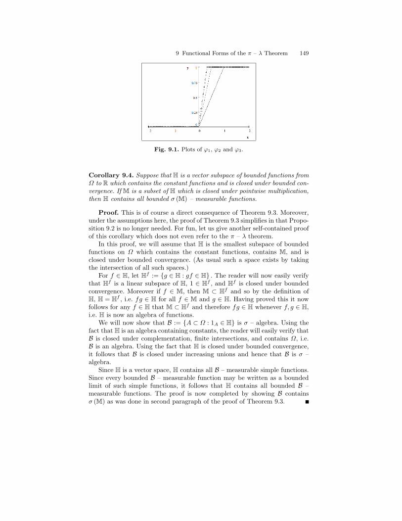
9 Functional Forms of the π – λ Theorem 149
Fig. 9.1. Plots of ϕ1, ϕ2 and ϕ3.
Corollary 9.4. Suppose that H is a vector subspace of bounded functions fromΩ to R which contains the constant functions and is closed under bounded con-vergence. If M is a subset of H which is closed under pointwise multiplication,then H contains all bounded σ (M) – measurable functions.
Proof. This is of course a direct consequence of Theorem 9.3. Moreover,under the assumptions here, the proof of Theorem 9.3 simplifies in that Propo-sition 9.2 is no longer needed. For fun, let us give another self-contained proofof this corollary which does not even refer to the π – λ theorem.
In this proof, we will assume that H is the smallest subspace of boundedfunctions on Ω which contains the constant functions, contains M, and isclosed under bounded convergence. (As usual such a space exists by takingthe intersection of all such spaces.)
For f ∈ H, let Hf := g ∈ H : gf ∈ H . The reader will now easily verifythat Hf is a linear subspace of H, 1 ∈ Hf , and Hf is closed under boundedconvergence. Moreover if f ∈ M, then M ⊂ Hf and so by the definition ofH, H = Hf , i.e. fg ∈ H for all f ∈ M and g ∈ H. Having proved this it nowfollows for any f ∈ H that M ⊂ Hf and therefore fg ∈ H whenever f, g ∈ H,i.e. H is now an algebra of functions.
We will now show that B := A ⊂ Ω : 1A ∈ H is σ – algebra. Using thefact that H is an algebra containing constants, the reader will easily verify thatB is closed under complementation, finite intersections, and contains Ω, i.e.B is an algebra. Using the fact that H is closed under bounded convergence,it follows that B is closed under increasing unions and hence that B is σ –algebra.
Since H is a vector space, H contains all B – measurable simple functions.Since every bounded B – measurable function may be written as a boundedlimit of such simple functions, it follows that H contains all bounded B –measurable functions. The proof is now completed by showing B containsσ (M) as was done in second paragraph of the proof of Theorem 9.3.

150 9 Functional Forms of the π – λ Theorem
Corollary 9.5. Suppose H is a real subspace of bounded functions such that1 ∈ H and H is closed under bounded convergence. If P ⊂ 2Ω is a multiplica-tive class such that 1A ∈ H for all A ∈ P, then H contains all bounded σ(P)– measurable functions.
Proof. Let M = 1 ∪ 1A : A ∈ P . Then M ⊂ H is a multiplicativesystem and the proof is completed with an application of Theorem 9.3.
Example 9.6. Suppose µ and ν are two probability measure on (Ω,B) suchthat ∫
Ω
fdµ =∫
Ω
fdν (9.1)
for all f in a multiplicative subset, M, of bounded measurable functions onΩ. Then µ = ν on σ (M) . Indeed, apply Theorem 9.3 with H being thebounded measurable functions on Ω such that Eq. (9.1) holds. In particularif M = 1 ∪ 1A : A ∈ P with P being a multiplicative class we learn thatµ = ν on σ (M) = σ (P) .
Corollary 9.7. The smallest subspace of real valued functions, H, on R whichcontains Cc (R,R) (the space of continuous functions on R with compact sup-port) is the collection of bounded Borel measurable function on R.
Proof. By a homework problem, for −∞ < a < b < ∞, 1(a,b] may bewritten as a bounded limit of continuous functions with compact supportfrom which it follows that σ (Cc(R,R)) = BR. It is also easy to see that 1is a bounded limit of functions in Cc(R,R) and hence 1 ∈ H. The corollarynow follows by an application of The result now follows by an application ofTheorem 9.3 with M := Cc(R,R).
For the rest of this chapter, recall for p ∈ [1,∞) that Lp(µ) = Lp(X,B, µ) isthe set of measurable functions f : Ω → R such that ‖f‖Lp :=
(∫|f |p dµ
)1/p<
∞. It is easy to see that ‖λf‖p = |λ| ‖f‖p for all λ ∈ R and we will show belowthat
‖f + g‖p ≤ ‖f‖p + ‖g‖p for all f, g ∈ Lp (µ) ,
i.e. ‖·‖p satisfies the triangle inequality.
Theorem 9.8 (Density Theorem). Let p ∈ [1,∞), (Ω,B, µ) be a measurespace and M be an algebra of bounded R – valued measurable functions suchthat
1. M ⊂ Lp (µ,R) and σ (M) = B.2. There exists ψk ∈ M such that ψk → 1 boundedly.
Then to every function f ∈ Lp (µ,R) , there exist ϕn ∈ M such thatlimn→∞ ‖f − ϕn‖Lp(µ) = 0, i.e. M is dense in Lp (µ,R) .

9 Functional Forms of the π – λ Theorem 151
Proof. Fix k ∈ N for the moment and let H denote those bounded B –measurable functions, f : Ω → R, for which there exists ϕn∞n=1 ⊂ M suchthat limn→∞ ‖ψkf − ϕn‖Lp(µ) = 0. A routine check shows H is a subspace ofthe bounded measurable R – valued functions on Ω, 1 ∈ H, M ⊂ H and His closed under bounded convergence. To verify the latter assertion, supposefn ∈ H and fn → f boundedly. Then, by the dominated convergence theorem,limn→∞ ‖ψk (f − fn)‖Lp(µ) = 0.1 (Take the dominating function to be g =[2C |ψk|]p where C is a constant bounding all of the |fn|∞n=1 .) We may nowchoose ϕn ∈ M such that ‖ϕn − ψkfn‖Lp(µ) ≤
1n then
lim supn→∞
‖ψkf − ϕn‖Lp(µ) ≤ lim supn→∞
‖ψk (f − fn)‖Lp(µ)
+ lim supn→∞
‖ψkfn − ϕn‖Lp(µ) = 0 (9.2)
which implies f ∈ H.An application of Dynkin’s Multiplicative System Theorem 9.3, now shows
H contains all bounded measurable functions on Ω. Let f ∈ Lp (µ) be given.The dominated convergence theorem implies limk→∞
∥∥ψk1|f |≤kf − f∥∥
Lp(µ)=
0. (Take the dominating function to be g = [2C |f |]p where C is a bound onall of the |ψk| .) Using this and what we have just proved, there exists ϕk ∈ Msuch that ∥∥ψk1|f |≤kf − ϕk
∥∥Lp(µ)
≤ 1k.
The same line of reasoning used in Eq. (9.2) now implies limk→∞ ‖f − ϕk‖Lp(µ) =0.
Example 9.9. Let µ be a measure on (R,BR) such that µ ([−M,M ]) < ∞ forall M < ∞. Then, Cc (R,R) (the space of continuous functions on R withcompact support) is dense in Lp (µ) for all 1 ≤ p < ∞. To see this, applyTheorem 9.8 with M = Cc (R,R) and ψk := 1[−k,k].
Theorem 9.10. Suppose p ∈ [1,∞), A ⊂ B ⊂ 2Ω is an algebra such thatσ(A) = B and µ is σ – finite on A. Let S(A, µ) denote the measurable simplefunctions, ϕ : Ω → R such ϕ = y ∈ A for all y ∈ R and µ (ϕ 6= 0) < ∞.Then S(A, µ) is dense subspace of Lp(µ).
Proof. Let M := S(A, µ). By assumption there exists Ωk ∈ A such thatµ(Ωk) < ∞ and Ωk ↑ Ω as k → ∞. If A ∈ A, then Ωk ∩ A ∈ A andµ (Ωk ∩A) <∞ so that 1Ωk∩A ∈ M. Therefore 1A = limk→∞ 1Ωk∩A is σ (M)– measurable for every A ∈ A. So we have shown that A ⊂ σ (M) ⊂ B andtherefore B = σ (A) ⊂ σ (M) ⊂ B, i.e. σ (M) = B. The theorem now followsfrom Theorem 9.8 after observing ψk := 1Ωk
∈ M and ψk → 1 boundedly.
1 It is at this point that the proof would break down if p = ∞.

152 9 Functional Forms of the π – λ Theorem
Theorem 9.11 (Separability of Lp – Spaces). Suppose, p ∈ [1,∞), A ⊂ Bis a countable algebra such that σ(A) = B and µ is σ – finite on A. Then Lp(µ)is separable and
D = ∑
aj1Aj : aj ∈ Q + iQ, Aj ∈ A with µ(Aj) <∞
is a countable dense subset.
Proof. It is left to reader to check D is dense in S(A, µ) relative to theLp(µ) – norm. Once this is done, the proof is then complete since S(A, µ) isa dense subspace of Lp (µ) by Theorem 9.10.
Notation 9.12 Given a collection of bounded functions, M, from a set, Ω,to R, let M↑ (M↓) denote the the bounded monotone increasing (decreasing)limits of functions from M. More explicitly a bounded function, f : Ω → Ris in M↑ respectively M↓ iff there exists fn ∈ M such that fn ↑ f respectivelyfn ↓ f.
Exercise 9.1. Let (Ω,B, P ) be a probability space and X,Y : Ω → R be apair of random variables such that
E [f (X) g (Y )] = E [f (X) g (X)]
for every pair of bounded measurable functions, f, g : R → R. ShowP (X = Y ) = 1. Hint: Let H denote the bounded Borel measurable func-tions, h : R2 → R such that
E [h (X,Y )] = E [h (X,X)] .
Use Corollary 9.4 to show H is the vector space of all bounded Borel measur-able functions. Then take h (x, y) = 1x=y.
Theorem 9.13 (Bounded Approximation Theorem). Let (Ω,B, µ) be afinite measure space and M be an algebra of bounded R – valued measurablefunctions such that:
1. σ (M) = B,2. 1 ∈ M, and3. |f | ∈ M for all f ∈ M.
Then for every bounded σ (M) measurable function, g : Ω → R, and everyε > 0, there exists f ∈ M↓ and h ∈ M↑ such that f ≤ g ≤ h and µ (h− f) < ε.Rework the Daniel
integral section inthe Analysis notes tostick to latticies ofbounded functions.
Proof. Let us begin with a few simple observations.
1. M is a “lattice” – if f, g ∈ M then
f ∨ g =12
(f + g + |f − g|) ∈ M
andf ∧ g =
12
(f + g − |f − g|) ∈ M.
9 Functional Forms of the π – λ Theorem 153
2. If f, g ∈ M↑ or f, g ∈ M↓ then f + g ∈ M↑ or f + g ∈ M↓ respectively.3. If λ ≥ 0 and f ∈ M↑ (f ∈ M↓), then λf ∈ M↑ (λf ∈ M↓) .4. If f ∈ M↑ then −f ∈ M↓ and visa versa.5. If fn ∈ M↑ and fn ↑ f where f : Ω → R is a bounded function, thenf ∈ M↑. Indeed, by assumption there exists fn,i ∈ M such that fn,i ↑ fn
as i → ∞. By observation (1), gn := max fij : i, j ≤ n ∈ M. Moreoverit is clear that gn ≤ max fk : k ≤ n = fn ≤ f and hence gn ↑ g :=limn→∞ gn ≤ f. Since fij ≤ g for all i, j, it follows that fn = limj→∞ fnj ≤g and consequently that f = limn→∞ fn ≤ g ≤ f. So we have shown thatgn ↑ f ∈ M↑.
Now let H denote the collection of bounded measurable functions whichsatisfy the assertion of the theorem. Clearly, M ⊂ H and in fact it is alsoeasy to see that M↑ and M↓ are contained in H as well. For example, iff ∈ M↑, by definition, there exists fn ∈ M ⊂ M↓ such that fn ↑ f. SinceM↓ 3 fn ≤ f ≤ f ∈ M↑ and µ (f − fn) → 0 by the dominated convergencetheorem, it follows that f ∈ H. As similar argument shows M↓ ⊂ H. We willnow show H is a vector sub-space of the bounded B = σ (M) – measurablefunctions.
H is closed under addition. If gi ∈ H for i = 1, 2, and ε > 0 is given, wemay find fi ∈ M↓ and hi ∈ M↑ such that fi ≤ gi ≤ hi and µ (hi − fi) < ε/2for i = 1, 2. Since h = h1 + h2 ∈ M↑, f := f1 + f2 ∈ M↓, f ≤ g1 + g2 ≤ h, and
µ (h− f) = µ (h1 − f1) + µ (h2 − f2) < ε,
it follows that g1 + g2 ∈ H.H is closed under scalar multiplication. If g ∈ H then λg ∈ H for all
λ ∈ R. Indeed suppose that ε > 0 is given and f ∈ M↓ and h ∈ M↑ such thatf ≤ g ≤ h and µ (h− f) < ε. Then for λ ≥ 0, M↓ 3 λf ≤ λg ≤ λh ∈ M↑ and
µ (λh− λf) = λµ (h− f) < λε.
Since ε > 0 was arbitrary, if follows that λg ∈ H for λ ≥ 0. Similarly, M↓ 3−h ≤ −g ≤ −f ∈ M↑ and
µ (−f − (−h)) = µ (h− f) < ε.
which shows −g ∈ H as well.Because of Theorem 9.3, to complete this proof, it suffices to show H is
closed under monotone convergence. So suppose that gn ∈ H and gn ↑ g,where g : Ω → R is a bounded function. Since H is a vector space, it followsthat 0 ≤ δn := gn+1 − gn ∈ H for all n ∈ N. So if ε > 0 is given, we canfind, M↓ 3 un ≤ δn ≤ vn ∈ M↑ such that µ (vn − un) ≤ 2−nε for all n. Byreplacing un by un ∨ 0 ∈ M↓ (by observation 1.), we may further assume thatun ≥ 0. Let
v :=∞∑
n=1
vn =↑ limN→∞
N∑n=1
vn ∈ M↑ (using observations 2. and 5.)

154 9 Functional Forms of the π – λ Theorem
and for N ∈ N, let
uN :=N∑
n=1
un ∈ M↓ (using observation 2).
Then∞∑
n=1
δn = limN→∞
N∑n=1
δn = limN→∞
(gN+1 − g1) = g − g1
and uN ≤ g − g1 ≤ v. Moreover,
µ(v − uN
)=
N∑n=1
µ (vn − un) +∞∑
n=N+1
µ (vn) ≤N∑
n=1
ε2−n +∞∑
n=N+1
µ (vn)
≤ ε+∞∑
n=N+1
µ (vn) .
However, since
∞∑n=1
µ (vn) ≤∞∑
n=1
µ(δn + ε2−n
)=∞∑
n=1
µ (δn) + εµ (Ω)
=∞∑
n=1
µ (g − g1) + εµ (Ω) <∞,
it follows that for N ∈ N sufficiently large that∑∞
n=N+1 µ (vn) < ε. Therefore,for this N, we have µ
(v − uN
)< 2ε and since ε > 0 is arbitrary, if follows
that g − g1 ∈ H. Since g1 ∈ H and H is a vector space, we may conclude thatg = (g − g1) + g1 ∈ H.
Theorem 9.14 (Complex Multiplicative System Theorem). SupposeH is a complex linear subspace of the bounded complex functions on Ω, 1 ∈ H,H is closed under complex conjugation, and H is closed under bounded conver-gence. If M ⊂ H is multiplicative system which is closed under conjugation,then H contains all bounded complex valued σ(M)-measurable functions.
Proof. Let M0 = spanC(M ∪ 1) be the complex span of M. As thereader should verify, M0 is an algebra, M0 ⊂ H, M0 is closed under complexconjugation and σ (M0) = σ (M) . Let
HR := f ∈ H : f is real valued and
MR0 := f ∈ M0 : f is real valued .
Then HR is a real linear space of bounded real valued functions 1 which isclosed under bounded convergence and MR
0 ⊂ HR. Moreover, MR0 is a multi-
plicative system (as the reader should check) and therefore by Theorem 9.3,

9 Functional Forms of the π – λ Theorem 155
HR contains all bounded σ(MR
0
)– measurable real valued functions. Since H
and M0 are complex linear spaces closed under complex conjugation, for anyf ∈ H or f ∈ M0, the functions Re f = 1
2
(f + f
)and Im f = 1
2i
(f − f
)are in
H or M0 respectively. Therefore M0 = MR0 + iMR
0 , σ(MR
0
)= σ (M0) = σ (M) ,
and H = HR + iHR. Hence if f : Ω → C is a bounded σ (M) – measurablefunction, then f = Re f + i Im f ∈ H since Re f and Im f are in HR.

10
Multiple and Iterated Integrals
10.1 Iterated Integrals
Notation 10.1 (Iterated Integrals) If (X,M, µ) and (Y,N , ν) are twomeasure spaces and f : X × Y → C is a M ⊗ N – measurable function,the iterated integrals of f (when they make sense) are:∫
X
dµ(x)∫
Y
dν(y)f(x, y) :=∫
X
[∫Y
f(x, y)dν(y)]dµ(x)
and ∫Y
dν(y)∫
X
dµ(x)f(x, y) :=∫
Y
[∫X
f(x, y)dµ(x)]dν(y).
Notation 10.2 Suppose that f : X → C and g : Y → C are functions, letf ⊗ g denote the function on X × Y given by
f ⊗ g(x, y) = f(x)g(y).
Notice that if f, g are measurable, then f⊗g is (M⊗N ,BC) – measurable.To prove this let F (x, y) = f(x) and G(x, y) = g(y) so that f ⊗ g = F ·G willbe measurable provided that F and G are measurable. Now F = f π1 whereπ1 : X ×Y → X is the projection map. This shows that F is the compositionof measurable functions and hence measurable. Similarly one shows that G ismeasurable.
10.2 Tonelli’s Theorem and Product Measure
Theorem 10.3. Suppose (X,M, µ) and (Y,N , ν) are σ-finite measure spacesand f is a nonnegative (M⊗N ,BR) – measurable function, then for eachy ∈ Y,
x→ f(x, y) is M – B[0,∞] measurable, (10.1)
for each x ∈ X,
y → f(x, y) is N – B[0,∞] measurable, (10.2)

158 10 Multiple and Iterated Integrals
x→∫
Y
f(x, y)dν(y) is M – B[0,∞] measurable, (10.3)
y →∫
X
f(x, y)dµ(x) is N – B[0,∞] measurable, (10.4)
and ∫X
dµ(x)∫
Y
dν(y)f(x, y) =∫
Y
dν(y)∫
X
dµ(x)f(x, y). (10.5)
Proof. Suppose that E = A×B ∈ E := M×N and f = 1E . Then
f(x, y) = 1A×B(x, y) = 1A(x)1B(y)
and one sees that Eqs. (10.1) and (10.2) hold. Moreover∫Y
f(x, y)dν(y) =∫
Y
1A(x)1B(y)dν(y) = 1A(x)ν(B),
so that Eq. (10.3) holds and we have∫X
dµ(x)∫
Y
dν(y)f(x, y) = ν(B)µ(A). (10.6)
Similarly, ∫X
f(x, y)dµ(x) = µ(A)1B(y) and∫Y
dν(y)∫
X
dµ(x)f(x, y) = ν(B)µ(A)
from which it follows that Eqs. (10.4) and (10.5) hold in this case as well.For the moment let us now further assume that µ(X) <∞ and ν(Y ) <∞
and let H be the collection of all bounded (M⊗N ,BR) – measurable functionson X × Y such that Eqs. (10.1) – (10.5) hold. Using the fact that measurablefunctions are closed under pointwise limits and the dominated convergencetheorem (the dominating function always being a constant), one easily showsthat H closed under bounded convergence. Since we have just verified that1E ∈ H for all E in the π – class, E , it follows by Corollary 9.5 that H isthe space of all bounded (M⊗N ,BR) – measurable functions on X × Y.Moreover, if f : X × Y → [0,∞] is a (M⊗N ,BR) – measurable function, letfM = M ∧ f so that fM ↑ f as M →∞. Then Eqs. (10.1) – (10.5) hold withf replaced by fM for all M ∈ N. Repeated use of the monotone convergencetheorem allows us to pass to the limit M → ∞ in these equations to deducethe theorem in the case µ and ν are finite measures.
For the σ – finite case, choose Xn ∈ M, Yn ∈ N such that Xn ↑ X,Yn ↑ Y, µ(Xn) < ∞ and ν(Yn) < ∞ for all m,n ∈ N. Then define µm(A) =µ(Xm ∩A) and νn(B) = ν(Yn ∩B) for all A ∈M and B ∈ N or equivalentlydµm = 1Xm
dµ and dνn = 1Yndν. By what we have just proved Eqs. (10.1) –

10.2 Tonelli’s Theorem and Product Measure 159
(10.5) with µ replaced by µm and ν by νn for all (M⊗N ,BR) – measurablefunctions, f : X×Y → [0,∞]. The validity of Eqs. (10.1) – (10.5) then followsby passing to the limits m→∞ and then n→∞ making use of the monotoneconvergence theorem in the following context. For all u ∈ L+(X,M),∫
X
udµm =∫
X
u1Xmdµ ↑
∫X
udµ as m→∞,
and for all and v ∈ L+(Y,N ),∫Y
vdµn =∫
Y
v1Yndµ ↑∫
Y
vdµ as n→∞.
Corollary 10.4. Suppose (X,M, µ) and (Y,N , ν) are σ – finite measurespaces. Then there exists a unique measure π on M⊗N such that π(A×B) =µ(A)ν(B) for all A ∈M and B ∈ N . Moreover π is given by
π(E) =∫
X
dµ(x)∫
Y
dν(y)1E(x, y) =∫
Y
dν(y)∫
X
dµ(x)1E(x, y) (10.7)
for all E ∈M⊗N and π is σ – finite.
Proof. Notice that any measure π such that π(A × B) = µ(A)ν(B) forall A ∈ M and B ∈ N is necessarily σ – finite. Indeed, let Xn ∈ M andYn ∈ N be chosen so that µ(Xn) < ∞, ν(Yn) < ∞, Xn ↑ X and Yn ↑ Y,then Xn × Yn ∈ M⊗N , Xn × Yn ↑ X × Y and π(Xn × Yn) < ∞ for all n.The uniqueness assertion is a consequence of the combination of Exercises 4.5and 5.1 Proposition 4.26 with E = M×N . For the existence, it suffices toobserve, using the monotone convergence theorem, that π defined in Eq. (10.7)is a measure on M⊗N . Moreover this measure satisfies π(A×B) = µ(A)ν(B)for all A ∈M and B ∈ N from Eq. (10.6).
Notation 10.5 The measure π is called the product measure of µ and ν andwill be denoted by µ⊗ ν.
Theorem 10.6 (Tonelli’s Theorem). Suppose (X,M, µ) and (Y,N , ν) areσ – finite measure spaces and π = µ ⊗ ν is the product measure on M⊗N .If f ∈ L+(X × Y,M⊗N ), then f(·, y) ∈ L+(X,M) for all y ∈ Y, f(x, ·) ∈L+(Y,N ) for all x ∈ X,∫
Y
f(·, y)dν(y) ∈ L+(X,M),∫X
f(x, ·)dµ(x) ∈ L+(Y,N )
and ∫X×Y
f dπ =∫
X
dµ(x)∫
Y
dν(y)f(x, y) (10.8)
=∫
Y
dν(y)∫
X
dµ(x)f(x, y). (10.9)

160 10 Multiple and Iterated Integrals
Proof. By Theorem 10.3 and Corollary 10.4, the theorem holds whenf = 1E with E ∈ M ⊗ N . Using the linearity of all of the statements, thetheorem is also true for non-negative simple functions. Then using the mono-tone convergence theorem repeatedly along with the approximation Theorem6.34, one deduces the theorem for general f ∈ L+(X × Y,M⊗N ).
Example 10.7. In this example we are going to show, I :=∫
R e−x2/2dm (x) =√
2π. To this end we observe, using Tonelli’s theorem, that
I2 =[∫
Re−x2/2dm (x)
]2=∫
Re−y2/2
[∫Re−x2/2dm (x)
]dm (y)
=∫
R2e−(x2+y2)/2dm2 (x, y)
where m2 = m ⊗ m is “Lebesgue measure” on(R2,BR2 = BR ⊗ BR
). From
the monotone convergence theorem,
I2 = limR→∞
∫DR
e−(x2+y2)/2dπ (x, y)
where DR =(x, y) : x2 + y2 < R2
. Using the change of variables theorem
described in Section 10.5 below,1 we find∫DR
e−(x2+y2)/2dπ (x, y) =∫
(0,R)×(0,2π)
e−r2/2rdrdθ
= 2π∫ R
0
e−r2/2rdr = 2π(1− e−R2/2
).
From this we learn that
I2 = limR→∞
2π(1− e−R2/2
)= 2π
as desired.
10.3 Fubini’s Theorem
The following convention will be in force for the rest of this section.Convention: If (X,M, µ) is a measure space and f : X → C is a measur-
able but non-integrable function, i.e.∫
X|f | dµ = ∞, by convention we will de-
fine∫
Xfdµ := 0. However if f is a non-negative function (i.e. f : X → [0,∞])
is a non-integrable function we will still write∫
Xfdµ = ∞.
1 Alternatively, you can easily show that the integralR
DRfdm2 agrees with the
multiple integral in undergraduate analysis when f is continuous. Then use thechange of variables theorem from undergraduate analysis.

10.3 Fubini’s Theorem 161
Theorem 10.8 (Fubini’s Theorem). Suppose (X,M, µ) and (Y,N , ν) areσ – finite measure spaces, π = µ ⊗ ν is the product measure on M⊗N andf : X × Y → C is a M⊗N – measurable function. Then the following threeconditions are equivalent:∫
X×Y
|f | dπ <∞, i.e. f ∈ L1(π), (10.10)∫X
(∫Y
|f(x, y)| dν(y))dµ(x) <∞ and (10.11)∫
Y
(∫X
|f(x, y)| dµ(x))dν(y) <∞. (10.12)
If any one (and hence all) of these condition hold, then f(x, ·) ∈ L1(ν) for µ-a.e. x, f(·, y) ∈ L1(µ) for ν-a.e. y,
∫Yf(·, y)dv(y) ∈ L1(µ),
∫Xf(x, ·)dµ(x) ∈
L1(ν) and Eqs. (10.8) and (10.9) are still valid.
Proof. The equivalence of Eqs. (10.10) – (10.12) is a direct consequenceof Tonelli’s Theorem 10.6. Now suppose f ∈ L1(π) is a real valued functionand let
E :=x ∈ X :
∫Y
|f (x, y)| dν (y) = ∞. (10.13)
Then by Tonelli’s theorem, x →∫
Y|f (x, y)| dν (y) is measurable and hence
E ∈M. Moreover Tonelli’s theorem implies∫X
[∫Y
|f (x, y)| dν (y)]dµ (x) =
∫X×Y
|f | dπ <∞
which implies that µ (E) = 0. Let f± be the positive and negative parts of f,then using the above convention we have∫
Y
f (x, y) dν (y) =∫
Y
1Ec (x) f (x, y) dν (y)
=∫
Y
1Ec (x) [f+ (x, y)− f− (x, y)] dν (y)
=∫
Y
1Ec (x) f+ (x, y) dν (y)−∫
Y
1Ec (x) f− (x, y) dν (y) .
(10.14)
Noting that 1Ec (x) f± (x, y) = (1Ec ⊗ 1Y · f±) (x, y) is a positive M⊗N –measurable function, it follows from another application of Tonelli’s theoremthat x →
∫Yf (x, y) dν (y) is M – measurable, being the difference of two
measurable functions. Moreover∫X
∣∣∣∣∫Y
f (x, y) dν (y)∣∣∣∣ dµ (x) ≤
∫X
[∫Y
|f (x, y)| dν (y)]dµ (x) <∞,

162 10 Multiple and Iterated Integrals
which shows∫
Yf(·, y)dv(y) ∈ L1(µ). Integrating Eq. (10.14) on x and using
Tonelli’s theorem repeatedly implies,∫X
[∫Y
f (x, y) dν (y)]dµ (x)
=∫
X
dµ (x)∫
Y
dν (y) 1Ec (x) f+ (x, y)−∫
X
dµ (x)∫
Y
dν (y) 1Ec (x) f− (x, y)
=∫
Y
dν (y)∫
X
dµ (x) 1Ec (x) f+ (x, y)−∫
Y
dν (y)∫
X
dµ (x) 1Ec (x) f− (x, y)
=∫
Y
dν (y)∫
X
dµ (x) f+ (x, y)−∫
Y
dν (y)∫
X
dµ (x) f− (x, y)
=∫
X×Y
f+dπ −∫
X×Y
f−dπ =∫
X×Y
(f+ − f−) dπ =∫
X×Y
fdπ (10.15)
which proves Eq. (10.8) holds.Now suppose that f = u + iv is complex valued and again let E be as
in Eq. (10.13). Just as above we still have E ∈ M and µ (E) = 0. By ourconvention,∫
Y
f (x, y) dν (y) =∫
Y
1Ec (x) f (x, y) dν (y) =∫
Y
1Ec (x) [u (x, y) + iv (x, y)] dν (y)
=∫
Y
1Ec (x)u (x, y) dν (y) + i
∫Y
1Ec (x) v (x, y) dν (y)
which is measurable in x by what we have just proved. Similarly one shows∫Yf (·, y) dν (y) ∈ L1 (µ) and Eq. (10.8) still holds by a computation similar
to that done in Eq. (10.15). The assertions pertaining to Eq. (10.9) may beproved in the same way.
The previous theorems have obvious generalizations to products of anyfinite number of σ – finite measure spaces. For example the following theoremholds.
Theorem 10.9. Suppose (Xi,Mi, µi)ni=1 are σ – finite measure spaces
and X := X1 × · · · × Xn. Then there exists a unique measure, π, on(X,M1 ⊗ · · · ⊗Mn) such that
π(A1 × · · · ×An) = µ1(A1) . . . µn(An) for all Ai ∈Mi.
(This measure and its completion will be denoted by µ1⊗· · ·⊗µn.) If f : X →[0,∞] is a M1 ⊗ · · · ⊗Mn – measurable function then∫
X
fdπ =∫
Xσ(1)
dµσ(1)(xσ(1)) . . .∫
Xσ(n)
dµσ(n)(xσ(n)) f(x1, . . . , xn) (10.16)
where σ is any permutation of 1, 2, . . . , n. This equation also holds for anyf ∈ L1(π) and moreover, f ∈ L1(π) iff
10.3 Fubini’s Theorem 163∫Xσ(1)
dµσ(1)(xσ(1)) . . .∫
Xσ(n)
dµσ(n)(xσ(n)) |f(x1, . . . , xn)| <∞
for some (and hence all) permutations, σ.
This theorem can be proved by the same methods as in the two factor case,see Exercise 10.4. Alternatively, one can use the theorems already proved andinduction on n, see Exercise 10.5 in this regard.
Proposition 10.10. Suppose that Xknk=1 are random variables on a prob-
ability space (Ω,B, P ) and µk = P X−1k is the distribution for Xk for
k = 1, 2, . . . , n, and π := P (X1, . . . , Xn)−1 is the joint distribution of(X1, . . . , Xn) . Then the following are equivalent,
1. Xknk=1 are independent,
2. for all bounded measurable functions, f : (Rn,BRn) → (R,BR) ,
Ef (X1, . . . , Xn) =∫
Rn
f (x1, . . . , xn) dµ1 (x1) . . . dµn (xn) , (taken in any order)
(10.17)and
3. π = µ1 ⊗ µ2 ⊗ · · · ⊗ µn.
Proof. (1 =⇒ 2) Suppose that Xknk=1 are independent and let H de-
note the set of bounded measurable functions, f : (Rn,BRn) → (R,BR) suchthat Eq. (10.17) holds. Then it is easily checked that H is a vector spacewhich contains the constant functions and is closed under bounded conver-gence. Moreover, if f = 1A1×···×An
where Ai ∈ BR, we have
Ef (X1, . . . , Xn) = P ((X1, . . . , Xn) ∈ A1 × · · · ×An)
=n∏
j=1
P (Xj ∈ Aj) =n∏
j=1
µj (Aj)
=∫
Rn
f (x1, . . . , xn) dµ1 (x1) . . . dµn (xn) .
Therefore, H contains the multiplicative system, M := 1A1×···×An: Ai ∈ BR
and so by the multiplicative systems theorem, H contains all bounded σ (M) =BRn – measurable functions.
(2 =⇒ 3) Let A ∈ BRn and f = 1A in Eq. (10.17) to conclude that
π (A) = P ((X1, . . . , Xn) ∈ A) = E1A (X1, . . . , Xn)
=∫
Rn
1A (x1, . . . , xn) dµ1 (x1) . . . dµn (xn) = (µ1 ⊗ · · · ⊗ µn) (A) .
(3 =⇒ 1) This follows from the identity,
164 10 Multiple and Iterated Integrals
P ((X1, . . . , Xn) ∈ A1 × · · · ×An) = π (A1 × · · · ×An) =n∏
j=1
µj (Aj)
=n∏
j=1
P (Xj ∈ Aj) ,
which is valid for all Aj ∈ BR.
Example 10.11 (No Ties). Suppose that X and Y are independent randomvariables on a probability space (Ω,B, P ) . If F (x) := P (X ≤ x) is con-tinuous, then P (X = Y ) = 0. To prove this, let µ (A) := P (X ∈ A) andν (A) = P (Y ∈ A) . Because F is continuous, µ (y) = F (y) − F (y−) = 0,and hence
P (X = Y ) = E[1X=Y
]=∫
R21x=yd (µ⊗ ν) (x, y)
=∫
Rdν (y)
∫Rdµ (x) 1x=y =
∫Rµ (y) dν (y)
=∫
R0 dν (y) = 0.
Example 10.12. In this example we will show
limM→∞
∫ M
0
sinxx
dx = π/2. (10.18)
To see this write 1x =
∫∞0e−txdt and use Fubini-Tonelli to conclude that∫ M
0
sinxx
dx =∫ M
0
[∫ ∞0
e−tx sinx dt]dx
=∫ ∞
0
[∫ M
0
e−tx sinx dx
]dt
=∫ ∞
0
11 + t2
(1− te−Mt sinM − e−Mt cosM
)dt
→∫ ∞
0
11 + t2
dt =π
2as M →∞,
wherein we have used the dominated convergence theorem (for instance, takeg (t) := 1
1+t2 (1 + te−t + e−t)) to pass to the limit.
The next example is a refinement of this result.
Example 10.13. We have∫ ∞0
sinxx
e−Λxdx =12π − arctanΛ for all Λ > 0 (10.19)

10.3 Fubini’s Theorem 165
and forΛ,M ∈ [0,∞),∣∣∣∣∣∫ M
0
sinxx
e−Λxdx− 12π + arctanΛ
∣∣∣∣∣ ≤ Ce−MΛ
M(10.20)
where C = maxx≥01+x1+x2 = 1
2√
2−2∼= 1.2. In particular Eq. (10.18) is valid.
To verify these assertions, first notice that by the fundamental theorem ofcalculus,
|sinx| =∣∣∣∣∫ x
0
cos ydy∣∣∣∣ ≤ ∣∣∣∣∫ x
0
|cos y| dy∣∣∣∣ ≤ ∣∣∣∣∫ x
0
1dy∣∣∣∣ = |x|
so∣∣ sin x
x
∣∣ ≤ 1 for all x 6= 0. Making use of the identity∫ ∞0
e−txdt = 1/x
and Fubini’s theorem,∫ M
0
sinxx
e−Λxdx =∫ M
0
dx sinx e−Λx
∫ ∞0
e−txdt
=∫ ∞
0
dt
∫ M
0
dx sinx e−(Λ+t)x
=∫ ∞
0
1− (cosM + (Λ+ t) sinM) e−M(Λ+t)
(Λ+ t)2 + 1dt
=∫ ∞
0
1(Λ+ t)2 + 1
dt−∫ ∞
0
cosM + (Λ+ t) sinM(Λ+ t)2 + 1
e−M(Λ+t)dt
=12π − arctanΛ− ε(M,Λ) (10.21)
where
ε(M,Λ) =∫ ∞
0
cosM + (Λ+ t) sinM(Λ+ t)2 + 1
e−M(Λ+t)dt.
Since ∣∣∣∣∣cosM + (Λ+ t) sinM(Λ+ t)2 + 1
∣∣∣∣∣ ≤ 1 + (Λ+ t)(Λ+ t)2 + 1
≤ C,
|ε(M,Λ)| ≤∫ ∞
0
e−M(Λ+t)dt = Ce−MΛ
M.
This estimate along with Eq. (10.21) proves Eq. (10.20) from which Eq. (10.18)follows by taking Λ → ∞ and Eq. (10.19) follows (using the dominated con-vergence theorem again) by letting M →∞.
Note: you may skip the rest of this chapter!

166 10 Multiple and Iterated Integrals
10.4 Fubini’s Theorem and Completions
Notation 10.14 Given E ⊂ X × Y and x ∈ X, let
xE := y ∈ Y : (x, y) ∈ E.
Similarly if y ∈ Y is given let
Ey := x ∈ X : (x, y) ∈ E.
If f : X × Y → C is a function let fx = f(x, ·) and fy := f(·, y) so thatfx : Y → C and fy : X → C.
Theorem 10.15. Suppose (X,M, µ) and (Y,N , ν) are complete σ – finitemeasure spaces. Let (X×Y,L, λ) be the completion of (X×Y,M⊗N , µ⊗ν). Iff is L – measurable and (a) f ≥ 0 or (b) f ∈ L1(λ) then fx is N – measurablefor µ a.e. x and fy is M – measurable for ν a.e. y and in case (b) fx ∈ L1(ν)and fy ∈ L1(µ) for µ a.e. x and ν a.e. y respectively. Moreover,(
x→∫
Y
fxdν
)∈ L1 (µ) and
(y →
∫X
fydµ
)∈ L1 (ν)
and ∫X×Y
fdλ =∫
Y
dν
∫X
dµ f =∫
X
dµ
∫Y
dν f.
Proof. If E ∈M⊗N is a µ⊗ ν null set (i.e. (µ⊗ ν)(E) = 0), then
0 = (µ⊗ ν)(E) =∫X
ν(xE)dµ(x) =∫X
µ(Ey)dν(y).
This shows that
µ(x : ν(xE) 6= 0) = 0 and ν(y : µ(Ey) 6= 0) = 0,
i.e. ν(xE) = 0 for µ a.e. x and µ(Ey) = 0 for ν a.e. y. If h is L measurable andh = 0 for λ – a.e., then there exists E ∈ M⊗N such that (x, y) : h(x, y) 6=0 ⊂ E and (µ⊗ν)(E) = 0. Therefore |h(x, y)| ≤ 1E(x, y) and (µ⊗ν)(E) = 0.Since
hx 6= 0 = y ∈ Y : h(x, y) 6= 0 ⊂ xE andhy 6= 0 = x ∈ X : h(x, y) 6= 0 ⊂ Ey
we learn that for µ a.e. x and ν a.e. y that hx 6= 0 ∈ M, hy 6= 0 ∈ N ,ν(hx 6= 0) = 0 and a.e. and µ(hy 6= 0) = 0. This implies
∫Yh(x, y)dν(y)
exists and equals 0 for µ a.e. x and similarly that∫
Xh(x, y)dµ(x) exists and
equals 0 for ν a.e. y. Therefore

10.5 Lebesgue Measure on Rd and the Change of Variables Theorem 167
0 =∫
X×Y
hdλ =∫
Y
(∫X
hdµ
)dν =
∫X
(∫Y
hdν
)dµ.
For general f ∈ L1(λ), we may choose g ∈ L1(M ⊗ N , µ ⊗ ν) such thatf(x, y) = g(x, y) for λ− a.e. (x, y). Define h := f − g. Then h = 0, λ− a.e.Hence by what we have just proved and Theorem 10.6 f = g + h has thefollowing properties:
1. For µ a.e. x, y → f(x, y) = g(x, y) + h(x, y) is in L1(ν) and∫Y
f(x, y)dν(y) =∫
Y
g(x, y)dν(y).
2. For ν a.e. y, x→ f(x, y) = g(x, y) + h(x, y) is in L1(µ) and∫X
f(x, y)dµ(x) =∫
X
g(x, y)dµ(x).
From these assertions and Theorem 10.6, it follows that∫X
dµ(x)∫
Y
dν(y)f(x, y) =∫
X
dµ(x)∫
Y
dν(y)g(x, y)
=∫
Y
dν(y)∫
Y
dν(x)g(x, y)
=∫
X×Y
g(x, y)d(µ⊗ ν)(x, y)
=∫
X×Y
f(x, y)dλ(x, y).
Similarly it is shown that∫Y
dν(y)∫
X
dµ(x)f(x, y) =∫
X×Y
f(x, y)dλ(x, y).
10.5 Lebesgue Measure on Rd and the Change ofVariables Theorem
Notation 10.16 Let
md :=d times︷ ︸︸ ︷
m⊗ · · · ⊗m on BRd =
d times︷ ︸︸ ︷BR ⊗ · · · ⊗ BR
be the d – fold product of Lebesgue measure m on BR. We will also use md
to denote its completion and let Ld be the completion of BRd relative to md.A subset A ∈ Ld is called a Lebesgue measurable set and md is called d –dimensional Lebesgue measure, or just Lebesgue measure for short.

168 10 Multiple and Iterated Integrals
Definition 10.17. A function f : Rd → R is Lebesgue measurable iff−1(BR) ⊂ Ld.
Notation 10.18 I will often be sloppy in the sequel and write m for md anddx for dm(x) = dmd(x), i.e.∫
Rd
f (x) dx =∫
Rd
fdm =∫
Rd
fdmd.
Hopefully the reader will understand the meaning from the context.
Theorem 10.19. Lebesgue measure md is translation invariant. Moreover md
is the unique translation invariant measure on BRd such that md((0, 1]d) = 1.
Proof. Let A = J1 × · · · × Jd with Ji ∈ BR and x ∈ Rd. Then
x+A = (x1 + J1)× (x2 + J2)× · · · × (xd + Jd)
and therefore by translation invariance of m on BR we find that
md(x+A) = m(x1 + J1) . . .m(xd + Jd) = m(J1) . . .m(Jd) = md(A)
and hence md(x + A) = md(A) for all A ∈ BRd since it holds for A in amultiplicative system which generates BRd . From this fact we see that themeasure md(x + ·) and md(·) have the same null sets. Using this it is easilyseen that m(x+A) = m(A) for all A ∈ Ld. The proof of the second assertionis Exercise 10.6.
Exercise 10.1. In this problem you are asked to show there is no reasonablenotion of Lebesgue measure on an infinite dimensional Hilbert space. To bemore precise, suppose H is an infinite dimensional Hilbert space and m is acountably additive measure on BH which is invariant under translationsand satisfies, m(B0(ε)) > 0 for all ε > 0. Show m(V ) = ∞ for all non-emptyopen subsets V ⊂ H.
Theorem 10.20 (Change of Variables Theorem). Let Ω ⊂o Rd be anopen set and T : Ω → T (Ω) ⊂o Rd be a C1 – diffeomorphism,2 see Figure10.1. Then for any Borel measurable function, f : T (Ω) → [0,∞],∫
Ω
f (T (x)) |detT ′ (x) |dx =∫
T (Ω)
f (y) dy, (10.22)
where T ′(x) is the linear transformation on Rd defined by T ′(x)v := ddt |0T (x+
tv). More explicitly, viewing vectors in Rd as columns, T ′ (x) may be repre-sented by the matrix2 That is T : Ω → T (Ω) ⊂o Rd is a continuously differentiable bijection and the
inverse map T−1 : T (Ω) → Ω is also continuously differentiable.

10.5 Lebesgue Measure on Rd and the Change of Variables Theorem 169
T ′ (x) =
∂1T1 (x) . . . ∂dT1 (x)...
. . ....
∂1Td (x) . . . ∂dTd (x)
, (10.23)
i.e. the i - j – matrix entry of T ′(x) is given by T ′(x)ij = ∂iTj(x) whereT (x) = (T1(x), . . . , Td(x))tr and ∂i = ∂/∂xi.
Fig. 10.1. The geometric setup of Theorem 10.20.
Remark 10.21. Theorem 10.20 is best remembered as the statement: if wemake the change of variables y = T (x) , then dy = |detT ′ (x) |dx. As usual,you must also change the limits of integration appropriately, i.e. if x rangesthrough Ω then y must range through T (Ω) .
Proof. The proof will be by induction on d. The case d = 1 was essentiallydone in Exercise 8.7. Nevertheless, for the sake of completeness let us give aproof here. Suppose d = 1, a < α < β < b such that [a, b] is a compactsubinterval of Ω. Then |detT ′| = |T ′| and∫
[a,b]
1T ((α,β]) (T (x)) |T ′ (x)| dx =∫
[a,b]
1(α,β] (x) |T ′ (x)| dx =∫ β
α
|T ′ (x)| dx.
If T ′ (x) > 0 on [a, b] , then∫ β
α
|T ′ (x)| dx =∫ β
α
T ′ (x) dx = T (β)− T (α)
= m (T ((α, β])) =∫
T ([a,b])
1T ((α,β]) (y) dy

170 10 Multiple and Iterated Integrals
while if T ′ (x) < 0 on [a, b] , then∫ β
α
|T ′ (x)| dx = −∫ β
α
T ′ (x) dx = T (α)− T (β)
= m (T ((α, β])) =∫
T ([a,b])
1T ((α,β]) (y) dy.
Combining the previous three equations shows∫[a,b]
f (T (x)) |T ′ (x)| dx =∫
T ([a,b])
f (y) dy (10.24)
whenever f is of the form f = 1T ((α,β]) with a < α < β < b. An applicationof Dynkin’s multiplicative system Theorem 9.3 then implies that Eq. (10.24)holds for every bounded measurable function f : T ([a, b]) → R. (Observe that|T ′ (x)| is continuous and hence bounded for x in the compact interval, [a, b] .)Recall that Ω =
∑Nn=1 (an, bn) where an, bn ∈ R∪±∞ for n = 1, 2, · · · < N
withN = ∞ possible. Hence if f : T (Ω) → R + is a Borel measurable functionand an < αk < βk < bn with αk ↓ an and βk ↑ bn, then by what we havealready proved and the monotone convergence theorem∫
Ω
1(an,bn) · (f T ) · |T ′|dm =∫Ω
(1T ((an,bn)) · f
) T · |T ′|dm
= limk→∞
∫Ω
(1T ([αk,βk]) · f
) T · |T ′| dm
= limk→∞
∫T (Ω)
1T ([αk,βk]) · f dm
=∫
T (Ω)
1T ((an,bn)) · f dm.
Summing this equality on n, then shows Eq. (10.22) holds.To carry out the induction step, we now suppose d > 1 and suppose the
theorem is valid with d being replaced by d−1. For notational compactness, letus write vectors in Rd as row vectors rather than column vectors. Nevertheless,the matrix associated to the differential, T ′ (x) , will always be taken to begiven as in Eq. (10.23).
Case 1. Suppose T (x) has the form
T (x) = (xi, T2 (x) , . . . , Td (x)) (10.25)
orT (x) = (T1 (x) , . . . , Td−1 (x) , xi) (10.26)

10.5 Lebesgue Measure on Rd and the Change of Variables Theorem 171
for some i ∈ 1, . . . , d . For definiteness we will assume T is as in Eq. (10.25),the case of T in Eq. (10.26) may be handled similarly. For t ∈ R, let it :Rd−1 → Rd be the inclusion map defined by
it (w) := wt := (w1, . . . , wi−1, t, wi+1, . . . , wd−1) ,
Ωt be the (possibly empty) open subset of Rd−1 defined by
Ωt :=w ∈ Rd−1 : (w1, . . . , wi−1, t, wi+1, . . . , wd−1) ∈ Ω
and Tt : Ωt → Rd−1 be defined by
Tt (w) = (T2 (wt) , . . . , Td (wt)) ,
see Figure 10.2. Expanding detT ′ (wt) along the first row of the matrix T ′ (wt)
Fig. 10.2. In this picture d = i = 3 and Ω is an egg-shaped region with an egg-shaped hole. The picture indicates the geometry associated with the map T andslicing the set Ω along planes where x3 = t.
shows|detT ′ (wt)| = |detT ′t (w)| .
Now by the Fubini-Tonelli Theorem and the induction hypothesis,

172 10 Multiple and Iterated Integrals∫Ω
f T |detT ′|dm =∫Rd
1Ω · f T |detT ′|dm
=∫Rd
1Ω (wt) (f T ) (wt) |detT ′ (wt) |dwdt
=∫
R
∫Ωt
(f T ) (wt) |detT ′ (wt) |dw
dt=∫
R
∫Ωt
f (t, Tt (w)) |detT ′t (w) |dw
dt=∫
R
∫Tt(Ωt)
f (t, z) dz
dt =∫
R
∫Rd−1
1T (Ω) (t, z) f (t, z) dz
dt=∫
T (Ω)
f (y) dy
wherein the last two equalities we have used Fubini-Tonelli along with theidentity;
T (Ω) =∑t∈R
T (it (Ω)) =∑t∈R
(t, z) : z ∈ Tt (Ωt) .
Case 2. (Eq. (10.22) is true locally.) Suppose that T : Ω → Rd is a generalmap as in the statement of the theorem and x0 ∈ Ω is an arbitrary point. Wewill now show there exists an open neighborhood W ⊂ Ω of x0 such that∫
W
f T |detT ′|dm =∫
T (W )
fdm
holds for all Borel measurable function, f : T (W ) → [0,∞]. Let Mi be the 1-iminor of T ′ (x0) , i.e. the determinant of T ′ (x0) with the first row and ith –column removed. Since
0 6= detT ′ (x0) =d∑
i=1
(−1)i+1∂iTj (x0) ·Mi,
there must be some i such that Mi 6= 0. Fix an i such that Mi 6= 0 and let,
S (x) := (xi, T2 (x) , . . . , Td (x)) . (10.27)
Observe that |detS′ (x0)| = |Mi| 6= 0. Hence by the inverse function Theorem,there exist an open neighborhood W of x0 such that W ⊂o Ω and S (W ) ⊂o
Rd and S : W → S (W ) is a C1 – diffeomorphism. Let R : S (W ) → T (W ) ⊂o
Rd to be the C1 – diffeomorphism defined by

10.5 Lebesgue Measure on Rd and the Change of Variables Theorem 173
R (z) := T S−1 (z) for all z ∈ S (W ) .
Because
(T1 (x) , . . . , Td (x)) = T (x) = R (S (x)) = R ((xi, T2 (x) , . . . , Td (x)))
for all x ∈W, if
(z1, z2, . . . , zd) = S (x) = (xi, T2 (x) , . . . , Td (x))
thenR (z) =
(T1
(S−1 (z)
), z2, . . . , zd
). (10.28)
Observe that S is a map of the form in Eq. (10.25), R is a map of the formin Eq. (10.26), T ′ (x) = R′ (S (x))S′ (x) (by the chain rule) and (by the mul-tiplicative property of the determinant)
|detT ′ (x)| = |detR′ (S (x)) | |detS′ (x)| ∀ x ∈W.
So if f : T (W ) → [0,∞] is a Borel measurable function, two applications ofthe results in Case 1. shows,∫
W
f T · |detT ′|dm =∫W
(f R · |detR′|) S · |detS′| dm
=∫
S(W )
f R · |detR′|dm =∫
R(S(W ))
fdm
=∫
T (W )
fdm
and Case 2. is proved.Case 3. (General Case.) Let f : Ω → [0,∞] be a general non-negative
Borel measurable function and let
Kn := x ∈ Ω : dist(x,Ωc) ≥ 1/n and |x| ≤ n .
Then each Kn is a compact subset of Ω and Kn ↑ Ω as n → ∞. Using thecompactness of Kn and case 2, for each n ∈ N, there is a finite open coverWn of Kn such that W ⊂ Ω and Eq. (10.22) holds with Ω replaced by W foreach W ∈ Wn. Let Wi∞i=1 be an enumeration of ∪∞n=1Wn and set W1 = W1
and Wi := Wi \ (W1 ∪ · · · ∪Wi−1) for all i ≥ 2. Then Ω =∑∞
i=1 Wi and byrepeated use of case 2.,

174 10 Multiple and Iterated Integrals∫Ω
f T |detT ′|dm =∞∑
i=1
∫Ω
1Wi· (f T ) · |detT ′|dm
=∞∑
i=1
∫Wi
[(1T(Wi)f
) T]· |detT ′|dm
=∞∑
i=1
∫T (Wi)
1T(Wi) · f dm =n∑
i=1
∫T (Ω)
1T(Wi) · f dm
=∫
T (Ω)
fdm.
Remark 10.22. When d = 1, one often learns the change of variables formulaas ∫ b
a
f (T (x))T ′ (x) dx =∫ T (b)
T (a)
f (y) dy (10.29)
where f : [a, b] → R is a continuous function and T is C1 – function definedin a neighborhood of [a, b] . If T ′ > 0 on (a, b) then T ((a, b)) = (T (a) , T (b))and Eq. (10.29) is implies Eq. (10.22) with Ω = (a, b) . On the other hand ifT ′ < 0 on (a, b) then T ((a, b)) = (T (b) , T (a)) and Eq. (10.29) is equivalentto ∫
(a,b)
f (T (x)) (− |T ′ (x)|) dx = −∫ T (a)
T (b)
f (y) dy = −∫
T ((a,b))
f (y) dy
which is again implies Eq. (10.22). On the other hand Eq. (10.29) is moregeneral than Eq. (10.22) since it does not require T to be injective. Thestandard proof of Eq. (10.29) is as follows. For z ∈ T ([a, b]) , let
F (z) :=∫ z
T (a)
f (y) dy.
Then by the chain rule and the fundamental theorem of calculus,∫ b
a
f (T (x))T ′ (x) dx =∫ b
a
F ′ (T (x))T ′ (x) dx =∫ b
a
d
dx[F (T (x))] dx
= F (T (x)) |ba =∫ T (b)
T (a)
f (y) dy.
An application of Dynkin’s multiplicative systems theorem now shows thatEq. (10.29) holds for all bounded measurable functions f on (a, b) . Thenby the usual truncation argument, it also holds for all positive measurablefunctions on (a, b) .

10.5 Lebesgue Measure on Rd and the Change of Variables Theorem 175
Example 10.23. Continuing the setup in Theorem 10.20, if A ∈ BΩ , then
m (T (A)) =∫
Rd
1T (A) (y) dy =∫
Rd
1T (A) (Tx) |detT ′ (x)| dx
=∫
Rd
1A (x) |detT ′ (x)| dx
wherein the second equality we have made the change of variables, y = T (x) .Hence we have shown
d (m T ) = |detT ′ (·)| dm.
In particular if T ∈ GL(d,R) = GL(Rd) – the space of d×d invertible matrices,then m T = |detT |m, i.e.
m (T (A)) = |detT |m (A) for allA ∈ BRd . (10.30)
This equation also shows that mT and m have the same null sets and hencethe equality in Eq. (10.30) is valid for any A ∈ Ld.
Exercise 10.2. Show that f ∈ L1(T (Ω) ,md
)iff∫
Ω
|f T | |detT ′|dm <∞
and if f ∈ L1(T (Ω) ,md
), then Eq. (10.22) holds.
Example 10.24 (Polar Coordinates). Suppose T : (0,∞) × (0, 2π) → R2 isdefined by
x = T (r, θ) = (r cos θ, r sin θ) ,
i.e. we are making the change of variable,
x1 = r cos θ and x2 = r sin θ for 0 < r <∞ and 0 < θ < 2π.
In this case
T ′(r, θ) =(
cos θ − r sin θsin θ r cos θ
)and therefore
dx = |detT ′(r, θ)| drdθ = rdrdθ.
Observing that
R2 \ T ((0,∞)× (0, 2π)) = ` := (x, 0) : x ≥ 0
has m2 – measure zero, it follows from the change of variables Theorem 10.20that ∫
R2f(x)dx =
∫ 2π
0
dθ
∫ ∞0
dr r · f(r (cos θ, sin θ)) (10.31)
for any Borel measurable function f : R2 → [0,∞].

176 10 Multiple and Iterated Integrals
Example 10.25 (Holomorphic Change of Variables). Suppose that f : Ω ⊂o
C ∼= R2→ C is an injective holomorphic function such that f ′ (z) 6= 0 for allz ∈ Ω. We may express f as
f (x+ iy) = U (x, y) + iV (x, y)
for all z = x+ iy ∈ Ω. Hence if we make the change of variables,
w = u+ iv = f (x+ iy) = U (x, y) + iV (x, y)
then
dudv =∣∣∣∣det
[Ux Uy
Vx Vy
]∣∣∣∣ dxdy = |UxVy − UyVx| dxdy.
Recalling that U and V satisfy the Cauchy Riemann equations, Ux = Vy andUy = −Vx with f ′ = Ux + iVx, we learn
UxVy − UyVx = U2x + V 2
x = |f ′|2 .
Thereforedudv = |f ′ (x+ iy)|2 dxdy.
Example 10.26. In this example we will evaluate the integral
I :=∫∫
Ω
(x4 − y4
)dxdy
whereΩ =
(x, y) : 1 < x2 − y2 < 2, 0 < xy < 1
,
see Figure 10.3. We are going to do this by making the change of variables,
Fig. 10.3. The region Ω consists of the two curved rectangular regions shown.

10.5 Lebesgue Measure on Rd and the Change of Variables Theorem 177
(u, v) := T (x, y) =(x2 − y2, xy
),
in which case
dudv =∣∣∣∣det
[2x −2yy x
]∣∣∣∣ dxdy = 2(x2 + y2
)dxdy
Notice that(x4 − y4
)=(x2 − y2
) (x2 + y2
)= u
(x2 + y2
)=
12ududv.
The function T is not injective on Ω but it is injective on each of its connectedcomponents. Let D be the connected component in the first quadrant so thatΩ = −D ∪D and T (±D) = (1, 2) × (0, 1) . The change of variables theoremthen implies
I± :=∫∫±D
(x4 − y4
)dxdy =
12
∫∫(1,2)×(0,1)
ududv =12u2
2|21 · 1 =
34
and therefore I = I+ + I− = 2 · (3/4) = 3/2.
Exercise 10.3 (Spherical Coordinates). Let T : (0,∞)×(0, π)×(0, 2π) →R3 be defined by
T (r, ϕ, θ) = (r sinϕ cos θ, r sinϕ sin θ, r cosϕ)= r (sinϕ cos θ, sinϕ sin θ, cosϕ) ,
see Figure 10.4. By making the change of variables x = T (r, ϕ, θ) , show
Fig. 10.4. The relation of x to (r, φ, θ) in spherical coordinates.

178 10 Multiple and Iterated Integrals∫R3f(x)dx =
∫ π
0
dϕ
∫ 2π
0
dθ
∫ ∞0
dr r2 sinϕ · f(T (r, ϕ, θ))
for any Borel measurable function, f : R3 → [0,∞].
Lemma 10.27. Let a > 0 and
Id(a) :=∫Rd
e−a|x|2dm(x).
Then Id(a) = (π/a)d/2.
Proof. By Tonelli’s theorem and induction,
Id(a) =∫
Rd−1×Re−a|y|2e−at2md−1(dy) dt
= Id−1(a)I1(a) = Id1 (a). (10.32)
So it suffices to compute:
I2(a) =∫R2
e−a|x|2dm(x) =∫
R2\0
e−a(x21+x2
2)dx1dx2.
Using polar coordinates, see Eq. (10.31), we find,
I2(a) =∫ ∞
0
dr r
∫ 2π
0
dθ e−ar2= 2π
∫ ∞0
re−ar2dr
= 2π limM→∞
∫ M
0
re−ar2dr = 2π lim
M→∞
e−ar2
−2a
∫ M
0
=2π2a
= π/a.
This shows that I2(a) = π/a and the result now follows from Eq. (10.32).
10.6 The Polar Decomposition of Lebesgue Measure
Let
Sd−1 = x ∈ Rd : |x|2 :=d∑
i=1
x2i = 1
be the unit sphere in Rd equipped with its Borel σ – algebra, BSd−1 andΦ : Rd \ 0 → (0,∞)×Sd−1 be defined by Φ(x) := (|x| , |x|−1
x). The inversemap, Φ−1 : (0,∞) × Sd−1 → Rd \ 0 , is given by Φ−1(r, ω) = rω. Since Φand Φ−1 are continuous, they are both Borel measurable. For E ∈ BSd−1 anda > 0, let
Ea := rω : r ∈ (0, a] and ω ∈ E = Φ−1((0, a]× E) ∈ BRd .

10.6 The Polar Decomposition of Lebesgue Measure 179
Definition 10.28. For E ∈ BSd−1 , let σ(E) := d · m(E1). We call σ thesurface measure on Sd−1.
It is easy to check that σ is a measure. Indeed if E ∈ BSd−1 , thenE1 = Φ−1 ((0, 1]× E) ∈ BRd so that m(E1) is well defined. Moreover ifE =
∑∞i=1Ei, then E1 =
∑∞i=1 (Ei)1 and
σ(E) = d ·m(E1) =∞∑
i=1
m ((Ei)1) =∞∑
i=1
σ(Ei).
The intuition behind this definition is as follows. If E ⊂ Sd−1 is a set andε > 0 is a small number, then the volume of
(1, 1 + ε] · E = rω : r ∈ (1, 1 + ε] and ω ∈ E
should be approximately given by m ((1, 1 + ε] · E) ∼= σ(E)ε, see Figure 10.5below. On the other hand
Fig. 10.5. Motivating the definition of surface measure for a sphere.
m ((1, 1 + ε]E) = m (E1+ε \ E1) =(1 + ε)d − 1
m(E1).
Therefore we expect the area of E should be given by
σ(E) = limε↓0
(1 + ε)d − 1
m(E1)
ε= d ·m(E1).
The following theorem is motivated by Example 10.24 and Exercise 10.3.
Theorem 10.29 (Polar Coordinates). If f : Rd → [0,∞] is a (BRd ,B)–measurable function then∫
Rd
f(x)dm(x) =∫
(0,∞)×Sd−1
f(rω)rd−1 drdσ(ω). (10.33)
180 10 Multiple and Iterated Integrals
In particular if f : R+ → R+ is measurable then∫Rd
f(|x|)dx =∫ ∞
0
f(r)dV (r) (10.34)
where V (r) = m (B(0, r)) = rdm (B(0, 1)) = d−1σ(Sd−1
)rd.
Proof. By Exercise 8.6,∫Rd
fdm =∫
Rd\0
(f Φ−1
) Φ dm =
∫(0,∞)×Sd−1
(f Φ−1
)d (Φ∗m) (10.35)
and therefore to prove Eq. (10.33) we must work out the measure Φ∗m onB(0,∞) ⊗ BSd−1 defined by
Φ∗m(A) := m(Φ−1(A)
)∀ A ∈ B(0,∞) ⊗ BSd−1 . (10.36)
If A = (a, b]× E with 0 < a < b and E ∈ BSd−1 , then
Φ−1(A) = rω : r ∈ (a, b] and ω ∈ E = bE1 \ aE1
wherein we have used Ea = aE1 in the last equality. Therefore by the basicscaling properties of m and the fundamental theorem of calculus,
(Φ∗m) ((a, b]× E) = m (bE1 \ aE1) = m(bE1)−m(aE1)
= bdm(E1)− adm(E1) = d ·m(E1)∫ b
a
rd−1dr. (10.37)
Letting dρ(r) = rd−1dr, i.e.
ρ(J) =∫
J
rd−1dr ∀ J ∈ B(0,∞), (10.38)
Eq. (10.37) may be written as
(Φ∗m) ((a, b]× E) = ρ((a, b]) · σ(E) = (ρ⊗ σ) ((a, b]× E) . (10.39)
SinceE = (a, b]× E : 0 < a < b and E ∈ BSd−1 ,
is a π class (in fact it is an elementary class) such that σ(E) = B(0,∞)⊗BSd−1 ,it follows from the π – λ Theorem and Eq. (10.39) that Φ∗m = ρ⊗ σ. Usingthis result in Eq. (10.35) gives∫
Rd
fdm =∫
(0,∞)×Sd−1
(f Φ−1
)d (ρ⊗ σ)
which combined with Tonelli’s Theorem 10.6 proves Eq. (10.35).
10.6 The Polar Decomposition of Lebesgue Measure 181
Corollary 10.30. The surface area σ(Sd−1) of the unit sphere Sd−1 ⊂ Rd is
σ(Sd−1) =2πd/2
Γ (d/2)(10.40)
where Γ is the gamma function given by
Γ (x) :=∫ ∞
0
ux−1e−udu (10.41)
Moreover, Γ (1/2) =√π, Γ (1) = 1 and Γ (x+ 1) = xΓ (x) for x > 0.
Proof. Using Theorem 10.29 we find
Id(1) =∫ ∞
0
dr rd−1e−r2∫
Sd−1
dσ = σ(Sd−1)∫ ∞
0
rd−1e−r2dr.
We simplify this last integral by making the change of variables u = r2 sothat r = u1/2 and dr = 1
2u−1/2du. The result is∫ ∞
0
rd−1e−r2dr =
∫ ∞0
ud−12 e−u 1
2u−1/2du
=12
∫ ∞0
ud2−1e−udu =
12Γ (d/2). (10.42)
Combing the the last two equations with Lemma 10.27 which states thatId(1) = πd/2, we conclude that
πd/2 = Id(1) =12σ(Sd−1)Γ (d/2)
which proves Eq. (10.40). Example 8.8 implies Γ (1) = 1 and from Eq. (10.42),
Γ (1/2) = 2∫ ∞
0
e−r2dr =
∫ ∞−∞
e−r2dr
= I1(1) =√π.
The relation, Γ (x+1) = xΓ (x) is the consequence of the following integrationby parts argument:
Γ (x+ 1) =∫ ∞
0
e−u ux+1 du
u=∫ ∞
0
ux
(− d
due−u
)du
= x
∫ ∞0
ux−1 e−u du = x Γ (x).
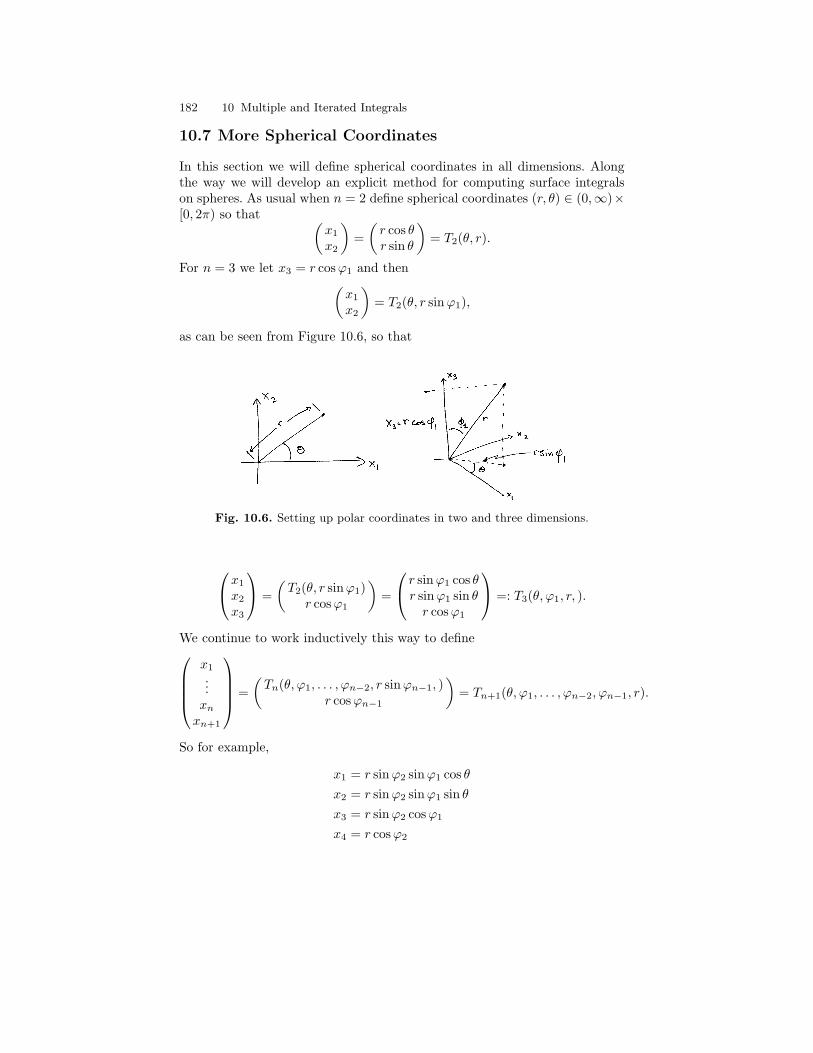
182 10 Multiple and Iterated Integrals
10.7 More Spherical Coordinates
In this section we will define spherical coordinates in all dimensions. Alongthe way we will develop an explicit method for computing surface integralson spheres. As usual when n = 2 define spherical coordinates (r, θ) ∈ (0,∞)×[0, 2π) so that (
x1
x2
)=(r cos θr sin θ
)= T2(θ, r).
For n = 3 we let x3 = r cosϕ1 and then(x1
x2
)= T2(θ, r sinϕ1),
as can be seen from Figure 10.6, so that
Fig. 10.6. Setting up polar coordinates in two and three dimensions.
x1
x2
x3
=(T2(θ, r sinϕ1)
r cosϕ1
)=
r sinϕ1 cos θr sinϕ1 sin θr cosϕ1
=: T3(θ, ϕ1, r, ).
We continue to work inductively this way to definex1
...xn
xn+1
=(Tn(θ, ϕ1, . . . , ϕn−2, r sinϕn−1, )
r cosϕn−1
)= Tn+1(θ, ϕ1, . . . , ϕn−2, ϕn−1, r).
So for example,
x1 = r sinϕ2 sinϕ1 cos θx2 = r sinϕ2 sinϕ1 sin θx3 = r sinϕ2 cosϕ1
x4 = r cosϕ2

10.7 More Spherical Coordinates 183
and more generally,
x1 = r sinϕn−2 . . . sinϕ2 sinϕ1 cos θx2 = r sinϕn−2 . . . sinϕ2 sinϕ1 sin θx3 = r sinϕn−2 . . . sinϕ2 cosϕ1
...xn−2 = r sinϕn−2 sinϕn−3 cosϕn−4
xn−1 = r sinϕn−2 cosϕn−3
xn = r cosϕn−2. (10.43)
By the change of variables formula,∫Rn
f(x)dm(x)
=∫ ∞
0
dr
∫0≤ϕi≤π,0≤θ≤2π
dϕ1 . . . dϕn−2dθ
[∆n(θ, ϕ1, . . . , ϕn−2, r)×f(Tn(θ, ϕ1, . . . , ϕn−2, r))
](10.44)
where∆n(θ, ϕ1, . . . , ϕn−2, r) := |detT ′n(θ, ϕ1, . . . , ϕn−2, r)| .
Proposition 10.31. The Jacobian, ∆n is given by
∆n(θ, ϕ1, . . . , ϕn−2, r) = rn−1 sinn−2 ϕn−2 . . . sin2 ϕ2 sinϕ1. (10.45)
If f is a function on rSn−1 – the sphere of radius r centered at 0 inside ofRn, then∫
rSn−1f(x)dσ(x) = rn−1
∫Sn−1
f(rω)dσ(ω)
=∫
0≤ϕi≤π,0≤θ≤2π
f(Tn(θ, ϕ1, . . . , ϕn−2, r))∆n(θ, ϕ1, . . . , ϕn−2, r)dϕ1 . . . dϕn−2dθ
(10.46)
Proof. We are going to compute ∆n inductively. Letting ρ := r sinϕn−1
and writing ∂Tn
∂ξ for ∂Tn
∂ξ (θ, ϕ1, . . . , ϕn−2, ρ) we have
∆n+1(θ,ϕ1, . . . , ϕn−2, ϕn−1, r)
=∣∣∣∣[ ∂Tn
∂θ∂Tn
∂ϕ1
0 0. . . ∂Tn
∂ϕn−2
. . . 0
∂Tn
∂ρ r cosϕn−1
−r sinϕn−1
∂Tn
∂ρ sinϕn−1
cosϕn−1
]∣∣∣∣= r
(cos2 ϕn−1 + sin2 ϕn−1
)∆n(, θ, ϕ1, . . . , ϕn−2, ρ)
= r∆n(θ, ϕ1, . . . , ϕn−2, r sinϕn−1),
i.e.
184 10 Multiple and Iterated Integrals
∆n+1(θ, ϕ1, . . . , ϕn−2, ϕn−1, r) = r∆n(θ, ϕ1, . . . , ϕn−2, r sinϕn−1). (10.47)
To arrive at this result we have expanded the determinant along the bottomrow. Staring with ∆2(θ, r) = r already derived in Example 10.24, Eq. (10.47)implies,
∆3(θ, ϕ1, r) = r∆2(θ, r sinϕ1) = r2 sinϕ1
∆4(θ, ϕ1, ϕ2, r) = r∆3(θ, ϕ1, r sinϕ2) = r3 sin2 ϕ2 sinϕ1
...
∆n(θ, ϕ1, . . . , ϕn−2, r) = rn−1 sinn−2 ϕn−2 . . . sin2 ϕ2 sinϕ1
which proves Eq. (10.45). Equation (10.46) now follows from Eqs. (10.33),(10.44) and (10.45).
As a simple application, Eq. (10.46) implies
σ(Sn−1) =∫
0≤ϕi≤π,0≤θ≤2π
sinn−2 ϕn−2 . . . sin2 ϕ2 sinϕ1dϕ1 . . . dϕn−2dθ
= 2πn−2∏k=1
γk = σ(Sn−2)γn−2 (10.48)
where γk :=∫ π
0sink ϕdϕ. If k ≥ 1, we have by integration by parts that,
γk =∫ π
0
sink ϕdϕ = −∫ π
0
sink−1 ϕ d cosϕ = 2δk,1 + (k − 1)∫ π
0
sink−2 ϕ cos2 ϕdϕ
= 2δk,1 + (k − 1)∫ π
0
sink−2 ϕ(1− sin2 ϕ
)dϕ = 2δk,1 + (k − 1) [γk−2 − γk]
and hence γk satisfies γ0 = π, γ1 = 2 and the recursion relation
γk =k − 1k
γk−2 for k ≥ 2.
Hence we may conclude
γ0 = π, γ1 = 2, γ2 =12π, γ3 =
232, γ4 =
34
12π, γ5 =
45
232, γ6 =
56
34
12π
and more generally by induction that
γ2k = π(2k − 1)!!
(2k)!!and γ2k+1 = 2
(2k)!!(2k + 1)!!
.
Indeed,
γ2(k+1)+1 =2k + 22k + 3
γ2k+1 =2k + 22k + 3
2(2k)!!
(2k + 1)!!= 2
[2(k + 1)]!!(2(k + 1) + 1)!!
10.7 More Spherical Coordinates 185
and
γ2(k+1) =2k + 12k + 1
γ2k =2k + 12k + 2
π(2k − 1)!!
(2k)!!= π
(2k + 1)!!(2k + 2)!!
.
The recursion relation in Eq. (10.48) may be written as
σ(Sn) = σ(Sn−1
)γn−1 (10.49)
which combined with σ(S1)
= 2π implies
σ(S1)
= 2π,
σ(S2) = 2π · γ1 = 2π · 2,
σ(S3) = 2π · 2 · γ2 = 2π · 2 · 12π =
22π2
2!!,
σ(S4) =22π2
2!!· γ3 =
22π2
2!!· 22
3=
23π2
3!!
σ(S5) = 2π · 2 · 12π · 2
32 · 3
412π =
23π3
4!!,
σ(S6) = 2π · 2 · 12π · 2
32 · 3
412π · 4
5232 =
24π3
5!!
and more generally that
σ(S2n) =2 (2π)n
(2n− 1)!!and σ(S2n+1) =
(2π)n+1
(2n)!!(10.50)
which is verified inductively using Eq. (10.49). Indeed,
σ(S2n+1) = σ(S2n)γ2n =2 (2π)n
(2n− 1)!!π
(2n− 1)!!(2n)!!
=(2π)n+1
(2n)!!
and
σ(S(n+1)) = σ(S2n+2) = σ(S2n+1)γ2n+1 =(2π)n+1
(2n)!!2
(2n)!!(2n+ 1)!!
=2 (2π)n+1
(2n+ 1)!!.
Using(2n)!! = 2n (2(n− 1)) . . . (2 · 1) = 2nn!
we may write σ(S2n+1) = 2πn+1
n! which shows that Eqs. (10.33) and (10.50 arein agreement. We may also write the formula in Eq. (10.50) as
σ(Sn) =
2(2π)n/2
(n−1)!! for n even(2π)
n+12
(n−1)!! for n odd.
186 10 Multiple and Iterated Integrals
10.8 Exercises
Exercise 10.4. Prove Theorem 10.9. Suggestion, to get started define
π (A) :=∫
X1
dµ (x1) . . .∫
Xn
dµ (xn) 1A (x1, . . . , xn)
and then show Eq. (10.16) holds. Use the case of two factors as the model ofyour proof.
Exercise 10.5. Let (Xj ,Mj , µj) for j = 1, 2, 3 be σ – finite measure spaces.Let F : (X1 ×X2)×X3 → X1 ×X2 ×X3 be defined by
F ((x1, x2), x3) = (x1, x2, x3).
1. Show F is ((M1 ⊗M2)⊗M3,M1 ⊗M2 ⊗M3) – measurable and F−1
is (M1 ⊗M2 ⊗M3, (M1 ⊗M2)⊗M3) – measurable. That is
F : ((X1 ×X2)×X3, (M1 ⊗M2)⊗M3) → (X1×X2×X3,M1⊗M2⊗M3)
is a “measure theoretic isomorphism.”2. Let π := F∗ [(µ1 ⊗ µ2)⊗ µ3] , i.e. π(A) = [(µ1 ⊗ µ2)⊗ µ3] (F−1(A)) for allA ∈M1 ⊗M2 ⊗M3. Then π is the unique measure on M1 ⊗M2 ⊗M3
such thatπ(A1 ×A2 ×A3) = µ1(A1)µ2(A2)µ3(A3)
for all Ai ∈Mi. We will write π := µ1 ⊗ µ2 ⊗ µ3.3. Let f : X1 ×X2 ×X3 → [0,∞] be a (M1 ⊗M2 ⊗M3,BR) – measurable
function. Verify the identity,∫X1×X2×X3
fdπ =∫
X3
dµ3(x3)∫
X2
dµ2(x2)∫
X1
dµ1(x1)f(x1, x2, x3),
makes sense and is correct.4. (Optional.) Also show the above identity holds for any one of the six
possible orderings of the iterated integrals.
Exercise 10.6. Prove the second assertion of Theorem 10.19. That is showmd is the unique translation invariant measure on BRd such that md((0, 1]d) =1. Hint: Look at the proof of Theorem 5.22.
Exercise 10.7. (Part of Folland Problem 2.46 on p. 69.) Let X = [0, 1],M = B[0,1] be the Borel σ – field on X, m be Lebesgue measure on [0, 1] andν be counting measure, ν(A) = #(A). Finally let D = (x, x) ∈ X2 : x ∈ Xbe the diagonal in X2. Show∫
X
[∫X
1D(x, y)dν(y)]dm(x) 6=
∫X
[∫X
1D(x, y)dm(x)]dν(y)
by explicitly computing both sides of this equation.

10.8 Exercises 187
Exercise 10.8. Folland Problem 2.48 on p. 69. (Counter example related toFubini Theorem involving counting measures.)
Exercise 10.9. Folland Problem 2.50 on p. 69 pertaining to area under acurve. (Note the M×BR should be M⊗BR in this problem.)
Exercise 10.10. Folland Problem 2.55 on p. 77. (Explicit integrations.)
Exercise 10.11. Folland Problem 2.56 on p. 77. Let f ∈ L1((0, a), dm),g(x) =
∫ a
xf(t)
t dt for x ∈ (0, a), show g ∈ L1((0, a), dm) and∫ a
0
g(x)dx =∫ a
0
f(t)dt.
Exercise 10.12. Show∫∞0
∣∣ sin xx
∣∣ dm(x) = ∞. So sin xx /∈ L1([0,∞),m) and∫∞
0sin x
x dm(x) is not defined as a Lebesgue integral.
Exercise 10.13. Folland Problem 2.57 on p. 77.
Exercise 10.14. Folland Problem 2.58 on p. 77.
Exercise 10.15. Folland Problem 2.60 on p. 77. Properties of the Γ – func-tion.
Exercise 10.16. Folland Problem 2.61 on p. 77. Fractional integration.
Exercise 10.17. Folland Problem 2.62 on p. 80. Rotation invariance of sur-face measure on Sn−1.
Exercise 10.18. Folland Problem 2.64 on p. 80. On the integrability of|x|a |log |x||b for x near 0 and x near ∞ in Rn.
Exercise 10.19. Show, using Problem 10.17 that∫Sd−1
ωiωjdσ (ω) =1dδijσ
(Sd−1
).
Hint: show∫
Sd−1 ω2i dσ (ω) is independent of i and therefore
∫Sd−1
ω2i dσ (ω) =
1d
d∑j=1
∫Sd−1
ω2jdσ (ω) .


11
Lp – spaces
Let (Ω,B, µ) be a measure space and for 0 < p <∞ and a measurable functionf : Ω → C let
‖f‖p :=(∫
Ω
|f |p dµ)1/p
(11.1)
and when p = ∞, let
‖f‖∞ = inf a ≥ 0 : µ(|f | > a) = 0 (11.2)
For 0 < p ≤ ∞, let
Lp(Ω,B, µ) = f : Ω → C : f is measurable and ‖f‖p <∞/ ∼
where f ∼ g iff f = g a.e. Notice that ‖f − g‖p = 0 iff f ∼ g and if f ∼ gthen ‖f‖p = ‖g‖p. In general we will (by abuse of notation) use f to denoteboth the function f and the equivalence class containing f.
Remark 11.1. Suppose that ‖f‖∞ ≤ M, then for all a > M, µ(|f | > a) = 0and therefore µ(|f | > M) = limn→∞ µ(|f | > M + 1/n) = 0, i.e. |f(ω)| ≤ Mfor µ - a.e. ω. Conversely, if |f | ≤M a.e. and a > M then µ(|f | > a) = 0 andhence ‖f‖∞ ≤M. This leads to the identity:
‖f‖∞ = inf a ≥ 0 : |f(ω)| ≤ a for µ – a.e. ω .
11.1 Modes of Convergence
Let fn∞n=1 ∪ f be a collection of complex valued measurable functions onΩ. We have the following notions of convergence and Cauchy sequences.
Definition 11.2. 1. fn → f a.e. if there is a set E ∈ B such that µ(E) = 0and limn→∞ 1Ecfn = 1Ecf.
2. fn → f in µ – measure if limn→∞ µ(|fn − f | > ε) = 0 for all ε > 0. Wewill abbreviate this by saying fn → f in L0 or by fn
µ→ f.3. fn → f in Lp iff f ∈ Lp and fn ∈ Lp for all n, and limn→∞ ‖fn − f‖p = 0.
Definition 11.3. 1. fn is a.e. Cauchy if there is a set E ∈ B such thatµ(E) = 0 and1Ec fn is a pointwise Cauchy sequences.

190 11 Lp – spaces
2. fn is Cauchy in µ – measure (or L0 – Cauchy) if limm,n→∞ µ(|fn −fm| > ε) = 0 for all ε > 0.
3. fn is Cauchy in Lp if limm,n→∞ ‖fn − fm‖p = 0.
When µ is a probability measure, we describe, fnµ→ f as fn converging
to f in probability. If a sequence fn∞n=1 is Lp – convergent, then it is Lp
– Cauchy. For example, when p ∈ [1,∞] and fn → f in Lp, we have
‖fn − fm‖p ≤ ‖fn − f‖p + ‖f − fm‖p → 0 as m,n→∞.
The case where p = 0 will be handled in Theorem 11.7 below.
Lemma 11.4 (Lp – convergence implies convergence in probability).Let p ∈ [1,∞). If fn ⊂ Lp is Lp – convergent (Cauchy) then fn is alsoconvergent (Cauchy) in measure.
Proof. By Chebyshev’s inequality (8.3),
µ (|f | ≥ ε) = µ (|f |p ≥ εp) ≤ 1εp
∫Ω
|f |p dµ =1εp‖f‖p
p
and therefore if fn is Lp – Cauchy, then
µ (|fn − fm| ≥ ε) ≤ 1εp‖fn − fm‖p
p → 0 as m,n→∞
showing fn is L0 – Cauchy. A similar argument holds for the Lp – convergentcase.
Here is a sequence of functions where fn → 0 a.e., fn 9 0 in L1, fnm→ 0.

11.1 Modes of Convergence 191
Above is a sequence of functions where fn → 0 a.e., yet fn 9 0 in L1. or inmeasure.
Here is a sequence of functions where fn → 0 a.e., fnm→ 0 but fn 9 0 in L1.

192 11 Lp – spaces
Above is a sequence of functions where fn → 0 in L1, fn 9 0 a.e., andfn
m→ 0.
Theorem 11.5 (Egoroff’s Theorem: almost sure convergence impliesconvergence in probability).
Suppose µ(Ω) = 1 and fn → f a.s. Then for all ε > 0 there exists E =Eε ∈ B such that µ(E) < ε and fn → f uniformly on Ec. In particularfn
µ−→ f as n→∞.
Proof. Let fn → f a.e. Then for all ε > 0,
0 = µ(|fn − f | > ε i.o. n)
= limN→∞
µ
⋃n≥N
|fn − f | > ε
(11.3)
≥ lim supN→∞
µ (|fN − f | > ε)
from which it follows that fnµ−→ f as n→∞. To get the uniform convergence
off a small exceptional set, the equality in Eq. (11.3) allows us to choose anincreasing sequence Nk∞k=1 , such that, if
Ek :=⋃
n≥Nk
|fn − f | > 1
k
, then µ(Ek) < ε2−k.
The set, E := ∪∞k=1Ek, then satisfies the estimate, µ(E) <∑
k ε2−k = ε.
Moreover, for ω /∈ E, we have |fn (ω)− f (ω)| ≤ 1k for all n ≥ Nk and all k.
That is fn → f uniformly on Ec.
Lemma 11.6. Suppose an ∈ C and |an+1 − an| ≤ εn and∞∑
n=1εn < ∞. Then
limn→∞
an = a ∈ C exists and |a− an| ≤ δn :=∞∑
k=n
εk.

11.1 Modes of Convergence 193
Proof. Let m > n then
|am − an| =∣∣∣∣m−1∑k=n
(ak+1 − ak)∣∣∣∣ ≤ m−1∑
k=n
|ak+1 − ak| ≤∞∑
k=n
εk := δn . (11.4)
So |am− an| ≤ δmin(m,n) → 0 as ,m, n→∞, i.e. an is Cauchy. Let m→∞in (11.4) to find |a− an| ≤ δn.
Theorem 11.7. Let (Ω,B, µ) be a measure space and fn∞n=1 be a sequenceof measurable functions on Ω.
1. If f and g are measurable functions and fnµ→ f and fn
µ→ g then f = ga.e.
2. If fnµ→ f then fn∞n=1 is Cauchy in measure.
3. If fn∞n=1 is Cauchy in measure, there exists a measurable function, f,and a subsequence gj = fnj
of fn such that limj→∞ gj := f exists a.e.4. If fn∞n=1 is Cauchy in measure and f is as in item 3. then fn
µ→ f.5. Let us now further assume that µ (Ω) < ∞. In this case, a sequence of
functions, fn∞n=1 converges to f in probability iff every subsequence,f ′n
∞n=1 of fn∞n=1 has a further subsequence, f ′′n
∞n=1 , which is almost
surely convergent to f.
Proof.
1. Suppose that f and g are measurable functions such that fnµ→ g and
fnµ→ f as n→∞ and ε > 0 is given. Since
|f − g| > ε = |f − fn + fn − g| > ε ⊂ |f − fn|+ |fn − g| > ε⊂ |f − fn| > ε/2 ∪ |g − fn| > ε/2 ,
µ(|f − g| > ε) ≤ µ(|f − fn| > ε/2) + µ(|g − fn| > ε/2) → 0 as n→∞.
Hence
µ(|f − g| > 0) = µ
(∪∞n=1
|f − g| > 1
n
)≤∞∑
n=1
µ
(|f − g| > 1
n
)= 0,
i.e. f = g a.e.2. Suppose fn
µ→ f, ε > 0 and m,n ∈ N and ω ∈ Ω are such that|fn (ω)− fm (ω)| > ε. Then
ε < |fn (ω)− fm (ω)| ≤ |fn (ω)− f (ω)|+ |f (ω)− fm (ω)|
from which it follows that either |fn (ω)− f (ω)| > ε/2 or |f (ω)− fm (ω)| >ε/2. Therefore we have shown,
|fn − fm| > ε ⊂ |fn − f | > ε/2 ∪ |fm − f | > ε/2
and hence
µ (|fn − fm| > ε) ≤ µ (|fn − f | > ε/2)+µ (|fm − f | > ε/2) → 0 as m,n→∞.

194 11 Lp – spaces
3. Suppose fn is L0 (µ) – Cauchy and let εn > 0 such that∞∑
n=1εn < ∞
(εn = 2−n would do) and set δn =∞∑
k=n
εk. Choose gj = fnjwhere nj is
a subsequence of N such that
µ(|gj+1 − gj | > εj) ≤ εj .
Let FN := ∪j≥N |gj+1 − gj | > εj and
E := ∩∞N=1FN = |gj+1 − gj | > εj i.o.
and observe that µ (FN ) ≤ δN <∞. Since
∞∑j=1
µ(|gj+1 − gj | > εj) ≤∞∑
j=1
εj <∞,
it follows from the first Borel-Cantelli lemma that
0 = µ (E) = limN→∞
µ (FN ) .
For ω /∈ E, |gj+1 (ω)− gj (ω)| ≤ εj for a.a. j and so by Lemma 11.6,f (ω) := lim
j→∞gj(ω) exists. For ω ∈ E we may define f (ω) ≡ 0.
4. Next we will show gNµ→ f as N →∞ where f and gN are as above. If
ω ∈ F cN = ∩j≥N |gj+1 − gj | ≤ εj ,
then|gj+1 (ω)− gj (ω)| ≤ εj for all j ≥ N.
Another application of Lemma 11.6 shows |f(ω)− gj(ω)| ≤ δj for allj ≥ N, i.e.
F cN ⊂ ∩j≥N ω ∈ Ω : |f(ω)− gj(ω)| ≤ δj .
Taking complements of this equation shows
|f − gN | > δN ⊂ ∪j≥N |f − gj | > δj ⊂ FN .
and therefore,
µ(|f − gN | > δN ) ≤ µ(FN ) ≤ δN → 0 as N →∞
and in particular, gNµ→ f as N →∞.
With this in hand, it is straightforward to show fnµ→ f. Indeed, since
|fn − f | > ε = |f − gj + gj − fn| > ε⊂ |f − gj |+ |gj − fn| > ε⊂ |f − gj | > ε/2 ∪ |gj − fn| > ε/2,
11.1 Modes of Convergence 195
we have
µ(|fn − f | > ε) ≤ µ(|f − gj | > ε/2) + µ(|gj − fn| > ε/2).
Therefore, letting j →∞ in this inequality gives,
µ(|fn − f | > ε) ≤ lim supj→∞
µ(|gj − fn| > ε/2) → 0 as n→∞
because fn∞n=1 was Cauchy in measure.5. If fn∞n=1 is convergent and hence Cauchy in probability then any sub-
sequence, f ′n∞n=1 is also Cauchy in probability. Hence by item 3. there
is a further subsequence, f ′′n∞n=1 of f ′n
∞n=1 which is convergent almost
surely.Conversely if fn∞n=1 does not converge to f in probability, then thereexists an ε > 0 and a subsequence, nk such that infk µ (|f − fnk
| ≥ ε) >0. Any subsequence of fnk
would have the same property and hence cannot be almost surely convergent because of Theorem 11.5.
Corollary 11.8 (Dominated Convergence Theorem). Let (Ω,B, µ) be ameasure space. Suppose fn , gn , and g are in L1 and f ∈ L0 are functionssuch that
|fn| ≤ gn a.e., fnµ−→ f, gn
µ−→ g, and∫gn →
∫g as n→∞.
Then f ∈ L1 and limn→∞ ‖f − fn‖1 = 0, i.e. fn → f in L1. In particularlimn→∞
∫fn =
∫f.
Proof. First notice that |f | ≤ g a.e. and hence f ∈ L1 since g ∈ L1. Tosee that |f | ≤ g, use Theorem 11.7 to find subsequences fnk
and gnk of
fn and gn respectively which are almost everywhere convergent. Then
|f | = limk→∞
|fnk| ≤ lim
k→∞gnk
= g a.e.
If (for sake of contradiction) limn→∞ ‖f − fn‖1 6= 0 there exists ε > 0 and asubsequence fnk
of fn such that∫|f − fnk
| ≥ ε for all k. (11.5)
Using Theorem 11.7 again, we may assume (by passing to a further subse-quences if necessary) that fnk
→ f and gnk→ g almost everywhere. Noting,
|f − fnk| ≤ g + gnk
→ 2g and∫
(g + gnk) →
∫2g, an application of the
dominated convergence Theorem 8.34 implies limk→∞∫|f − fnk
| = 0 whichcontradicts Eq. (11.5).

196 11 Lp – spaces
Exercise 11.1 (Fatou’s Lemma). Let (Ω,B, µ) be a measure space. If fn ≥0 and fn → f in measure, then
∫Ωfdµ ≤ lim infn→∞
∫Ωfndµ.
Exercise 11.2. Let (Ω,B, µ) be a measure space, p ∈ [1,∞), fn ⊂ Lp (µ)and f ∈ Lp (µ) . Then fn → f in Lp (µ) iff fn
µ−→ f and∫|fn|p →
∫|f |p .
Solution to Exercise (11.2). By the triangle inequality,∣∣∣‖f‖p − ‖fn‖p
∣∣∣ ≤‖f − fn‖p which shows
∫|fn|p →
∫|f |p if fn → f in Lp. Moreover
Chebyschev’s inequality implies fnµ−→ f if fn → f in Lp.
For the converse, let Fn := |f − fn|p and Gn := 2p−1 [|f |p + |fn|p] . ThenFn
µ−→ 0, Fn ≤ Gn ∈ L1, and∫Gn →
∫G where G := 2p |f |p ∈ L1.
Therefore, by Corollary 11.8,∫|f − fn|p =
∫Fn →
∫0 = 0.
Corollary 11.9. Suppose (Ω,B, µ) is a probability space, fnµ−→ f and gn
µ−→g and ϕ : R → R and ψ : R2 → R are continuous functions. Then
1. ϕ (fn)µ−→ ϕ (f) ,
2. ψ (fn, gn)µ−→ ψ (f, g) ,
3. fn + gnµ−→ f + g, and
4. fn · gnµ−→ f · g.
Proof. Item 1., 3. and 4. all follow from item 2. by taking ψ (x, y) = ϕ (x) ,ψ (x, y) = x+ y, and ψ (x, y) = x · y respectively. So it suffices to prove item2. To do this we will make repeated use of Theorem 11.7.
Given a subsequence, nk , of N there is a subsequence, n′k of nksuch that fn′k
→ f a.s. and yet a further subsequence n′′k of n′k such thatgn′′k
→ g a.s. Hence, by the continuity of ψ, it now follows that
limk→∞
ψ(fn′′k
, gn′′k
)= ψ (f, g) a.s.
which completes the proof.
11.2 Jensen’s, Holder’s and Minikowski’s Inequalities
Theorem 11.10 (Jensen’s Inequality). Suppose that (Ω,B, µ) is a prob-ability space, i.e. µ is a positive measure and µ(Ω) = 1. Also suppose thatf ∈ L1(µ), f : Ω → (a, b), and ϕ : (a, b) → R is a convex function, (i.e.ϕ′′ (x) ≥ 0 on (a, b) .) Then
ϕ
(∫Ω
fdµ
)≤∫
Ω
ϕ(f)dµ
where if ϕ f /∈ L1(µ), then ϕ f is integrable in the extended sense and∫Ωϕ(f)dµ = ∞.

11.2 Jensen’s, Holder’s and Minikowski’s Inequalities 197
Proof. Let t =∫
Ωfdµ ∈ (a, b) and let β ∈ R (β = ϕ (t) when ϕ (t) exists,
see Figure 7.2) be such that ϕ(s) − ϕ(t) ≥ β(s − t) for all s ∈ (a, b). Thenintegrating the inequality, ϕ(f)− ϕ(t) ≥ β(f − t), implies that
0 ≤∫
Ω
ϕ(f)dµ− ϕ(t) =∫
Ω
ϕ(f)dµ− ϕ(∫
Ω
fdµ).
Moreover, if ϕ(f) is not integrable, then ϕ(f) ≥ ϕ(t) + β(f − t) which showsthat negative part of ϕ(f) is integrable. Therefore,
∫Ωϕ(f)dµ = ∞ in this
case.
Example 11.11. Since ex for x ∈ R, − lnx for x > 0, and xp for x ≥ 0 andp ≥ 1 are all convex functions, we have the following inequalities
exp(∫
Ω
fdµ
)≤∫
Ω
efdµ, (11.6)∫Ω
log(|f |)dµ ≤ log(∫
Ω
|f | dµ)
and for p ≥ 1, ∣∣∣∣∫Ω
fdµ
∣∣∣∣p ≤ (∫Ω
|f | dµ)p
≤∫
Ω
|f |p dµ.
As a special case of Eq. (11.6), if pi, si > 0 for i = 1, 2, . . . , n and∑n
i=11pi
= 1,then
s1 . . . sn = ePn
i=1 ln si = ePn
i=11
piln s
pii ≤
n∑i=1
1pieln s
pii =
n∑i=1
spi
i
pi. (11.7)
Indeed, we have applied Eq. (11.6) with Ω = 1, 2, . . . , n , µ =∑n
i=11piδi and
f (i) := ln spi
i . As a special case of Eq. (11.7), suppose that s, t, p, q ∈ (1,∞)with q = p
p−1 (i.e. 1p + 1
q = 1) then
st ≤ 1psp +
1qtq. (11.8)
(When p = q = 1/2, the inequality in Eq. (11.8) follows from the inequality,0 ≤ (s− t)2 .)
As another special case of Eq. (11.7), take pi = n and si = a1/ni with
ai > 0, then we get the arithmetic geometric mean inequality,
n√a1 . . . an ≤
1n
n∑i=1
ai. (11.9)
Theorem 11.12 (Holder’s inequality). Suppose that 1 ≤ p ≤ ∞ and q :=p
p−1 , or equivalently p−1 + q−1 = 1. If f and g are measurable functions then

198 11 Lp – spaces
‖fg‖1 ≤ ‖f‖p · ‖g‖q. (11.10)
Assuming p ∈ (1,∞) and ‖f‖p · ‖g‖q < ∞, equality holds in Eq. (11.10) iff|f |p and |g|q are linearly dependent as elements of L1 which happens iff
|g|q‖f‖pp = ‖g‖q
q |f |p a.e. (11.11)
Proof. The cases p = 1 and q = ∞ or p = ∞ and q = 1 are easy to dealwith and will be left to the reader. So we now assume that p, q ∈ (1,∞) . If‖f‖q = 0 or ∞ or ‖g‖p = 0 or ∞, Eq. (11.10) is again easily verified. So we willnow assume that 0 < ‖f‖q, ‖g‖p <∞. Taking s = |f | /‖f‖p and t = |g|/‖g‖q
in Eq. (11.8) gives,
|fg|‖f‖p‖g‖q
≤ 1p
|f |p
‖f‖p+
1q
|g|q
‖g‖q(11.12)
with equality iff |g/‖g‖q| = |f |p−1/‖f‖(p−1)
p = |f |p/q/‖f‖p/q
p , i.e. |g|q‖f‖pp =
‖g‖qq |f |
p. Integrating Eq. (11.12) implies
‖fg‖1‖f‖p‖g‖q
≤ 1p
+1q
= 1
with equality iff Eq. (11.11) holds. The proof is finished since it is easilychecked that equality holds in Eq. (11.10) when |f |p = c |g|q of |g|q = c |f |pfor some constant c.
Example 11.13. Suppose that ak ∈ C for k = 1, 2, . . . , n and p ∈ [1,∞), then∣∣∣∣∣n∑
k=1
ak
∣∣∣∣∣p
≤ np−1n∑
k=1
|ak|p . (11.13)
Indeed, by Holder’s inequality applied using the measure space, 1, 2, . . . , nequipped with counting measure, we have∣∣∣∣∣
n∑k=1
ak
∣∣∣∣∣ =∣∣∣∣∣
n∑k=1
ak · 1
∣∣∣∣∣ ≤(
n∑k=1
|ak|p)1/p( n∑
k=1
1q
)1/q
= n1/q
(n∑
k=1
|ak|p)1/p
where q = pp−1 . Taking the pth – power of this inequality then gives, Eq.
(11.14).
Theorem 11.14 (Generalized Holder’s inequality). Suppose that fi :Ω → C are measurable functions for i = 1, . . . , n and p1, . . . , pn and r arepositive numbers such that
∑ni=1 p
−1i = r−1, then∥∥∥∥∥
n∏i=1
fi
∥∥∥∥∥r
≤n∏
i=1
‖fi‖pi. (11.14)

11.2 Jensen’s, Holder’s and Minikowski’s Inequalities 199
Proof. One may prove this theorem by induction based on Holder’s The-orem 11.12 above. Alternatively we may give a proof along the lines of theproof of Theorem 11.12 which is what we will do here.
Since Eq. (11.14) is easily seen to hold if ‖fi‖pi= 0 for some i, we will
assume that ‖fi‖pi> 0 for all i. By assumption,
∑ni=1
ri
pi= 1, hence we may
replace si by sri and pi by pi/r for each i in Eq. (11.7) to find
sr1 . . . s
rn ≤
n∑i=1
(sri )
pi/r
pi/r= r
n∑i=1
spi
i
pi.
Now replace si by |fi| / ‖fi‖piin the previous inequality and integrate the
result to find
1∏ni=1 ‖fi‖pi
∥∥∥∥∥n∏
i=1
fi
∥∥∥∥∥r
r
≤ rn∑
i=1
1pi
1‖fi‖pi
pi
∫Ω
|fi|pi dµ =n∑
i=1
r
pi= 1.
Theorem 11.15 (Minkowski’s Inequality). If 1 ≤ p ≤ ∞ and f, g ∈ Lp
then‖f + g‖p ≤ ‖f‖p + ‖g‖p. (11.15)
Proof. When p = ∞, |f | ≤ ‖f‖∞ a.e. and |g| ≤ ‖g‖∞ a.e. so that |f + g| ≤|f |+ |g| ≤ ‖f‖∞ + ‖g‖∞ a.e. and therefore
‖f + g‖∞ ≤ ‖f‖∞ + ‖g‖∞ .
When p <∞,
|f + g|p ≤ (2max (|f | , |g|))p = 2p max (|f |p , |g|p) ≤ 2p (|f |p + |g|p) ,
which implies1 f + g ∈ Lp since
‖f + g‖pp ≤ 2p
(‖f‖p
p + ‖g‖pp
)<∞.
Furthermore, when p = 1 we have
‖f + g‖1 =∫
Ω
|f + g|dµ ≤∫
Ω
|f | dµ+∫
Ω
|g|dµ = ‖f‖1 + ‖g‖1.
We now consider p ∈ (1,∞) . We may assume ‖f + g‖p, ‖f‖p and ‖g‖p areall positive since otherwise the theorem is easily verified. Integrating
|f + g|p = |f + g||f + g|p−1 ≤ (|f |+ |g|)|f + g|p−1
1 In light of Example 11.13, the last 2p in the above inequality may be replaced by2p−1.

200 11 Lp – spaces
and then applying Holder’s inequality with q = p/(p− 1) gives∫Ω
|f + g|pdµ ≤∫
Ω
|f | |f + g|p−1dµ+∫
Ω
|g| |f + g|p−1dµ
≤ (‖f‖p + ‖g‖p) ‖ |f + g|p−1 ‖q, (11.16)
where
‖|f + g|p−1‖qq =
∫Ω
(|f + g|p−1)qdµ =∫
Ω
|f + g|pdµ = ‖f + g‖pp. (11.17)
Combining Eqs. (11.16) and (11.17) implies
‖f + g‖pp ≤ ‖f‖p‖f + g‖p/q
p + ‖g‖p‖f + g‖p/qp (11.18)
Solving this inequality for ‖f + g‖p gives Eq. (11.15).
11.3 Completeness of Lp – spaces
Theorem 11.16. Let ‖·‖∞ be as defined in Eq. (11.2), then (L∞(Ω,B, µ), ‖·‖∞) isa Banach space. A sequence fn∞n=1 ⊂ L∞ converges to f ∈ L∞ iff there ex-ists E ∈ B such that µ(E) = 0 and fn → f uniformly on Ec. Moreover,bounded simple functions are dense in L∞.
Proof. By Minkowski’s Theorem 11.15, ‖·‖∞ satisfies the triangle inequal-ity. The reader may easily check the remaining conditions that ensure ‖·‖∞is a norm. Suppose that fn∞n=1 ⊂ L∞ is a sequence such fn → f ∈ L∞, i.e.‖f − fn‖∞ → 0 as n→∞. Then for all k ∈ N, there exists Nk <∞ such that
µ(|f − fn| > k−1
)= 0 for all n ≥ Nk.
LetE = ∪∞k=1 ∪n≥Nk
|f − fn| > k−1
.
Then µ(E) = 0 and for x ∈ Ec, |f(x)− fn(x)| ≤ k−1 for all n ≥ Nk. Thisshows that fn → f uniformly on Ec. Conversely, if there exists E ∈ B suchthat µ(E) = 0 and fn → f uniformly on Ec, then for any ε > 0,
µ (|f − fn| ≥ ε) = µ (|f − fn| ≥ ε ∩ Ec) = 0
for all n sufficiently large. That is to say lim supj→∞
‖f − fn‖∞ ≤ ε for all ε > 0.
The density of simple functions follows from the approximation Theorem 6.34.So the last item to prove is the completeness of L∞.
Suppose εm,n := ‖fm − fn‖∞ → 0 as m,n → ∞. Let Em,n =|fn − fm| > εm,n and E := ∪Em,n, then µ(E) = 0 and
supx∈Ec
|fm (x)− fn (x)| ≤ εm,n → 0 as m,n→∞.
Therefore, f := limn→∞ fn exists on Ec and the limit is uniform on Ec.Letting f = limn→∞ 1Ecfn, it then follows that limn→∞ ‖fn − f‖∞ = 0.

11.4 Relationships between different Lp – spaces 201
Theorem 11.17 (Completeness of Lp(µ)). For 1 ≤ p ≤ ∞, Lp(µ) equippedwith the Lp – norm, ‖·‖p (see Eq. (11.1)), is a Banach space.
Proof. By Minkowski’s Theorem 11.15, ‖·‖p satisfies the triangle inequal-ity. As above the reader may easily check the remaining conditions that ensure‖·‖p is a norm. So we are left to prove the completeness of Lp(µ) for 1 ≤ p <∞,the case p = ∞ being done in Theorem 11.16.
Let fn∞n=1 ⊂ Lp(µ) be a Cauchy sequence. By Chebyshev’s inequality(Lemma 11.4), fn is L0-Cauchy (i.e. Cauchy in measure) and by Theorem11.7 there exists a subsequence gj of fn such that gj → f a.e. By Fatou’sLemma,
‖gj − f‖pp =
∫lim
k→∞inf |gj − gk|pdµ ≤ lim
k→∞inf∫|gj − gk|pdµ
= limk→∞
inf ‖gj − gk‖pp → 0 as j →∞.
In particular, ‖f‖p ≤ ‖gj − f‖p + ‖gj‖p <∞ so the f ∈ Lp and gjLp
−→ f. Theproof is finished because,
‖fn − f‖p ≤ ‖fn − gj‖p + ‖gj − f‖p → 0 as j, n→∞.
See Proposition 12.5 for an important example of the use of this theorem.
11.4 Relationships between different Lp – spaces
The Lp(µ) – norm controls two types of behaviors of f, namely the “behaviorat infinity” and the behavior of “local singularities.” So in particular, if fblows up at a point x0 ∈ Ω, then locally near x0 it is harder for f to bein Lp(µ) as p increases. On the other hand a function f ∈ Lp(µ) is allowedto decay at “infinity” slower and slower as p increases. With these insightsin mind, we should not in general expect Lp(µ) ⊂ Lq(µ) or Lq(µ) ⊂ Lp(µ).However, there are two notable exceptions. (1) If µ(Ω) <∞, then there is nobehavior at infinity to worry about and Lq(µ) ⊂ Lp(µ) for all q ≥ p as is shownin Corollary 11.18 below. (2) If µ is counting measure, i.e. µ(A) = #(A), thenall functions in Lp(µ) for any p can not blow up on a set of positive measure,so there are no local singularities. In this case Lp(µ) ⊂ Lq(µ) for all q ≥ p,see Corollary 11.23 below.
Corollary 11.18. If µ(Ω) < ∞ and 0 < p < q ≤ ∞, then Lq(µ) ⊂ Lp(µ),the inclusion map is bounded and in fact
‖f‖p ≤ [µ(Ω)](1p−
1q ) ‖f‖q .

202 11 Lp – spaces
Proof. Take a ∈ [1,∞] such that
1p
=1a
+1q, i.e. a =
pq
q − p.
Then by Theorem 11.14,
‖f‖p = ‖f · 1‖p ≤ ‖f‖q · ‖1‖a = µ(Ω)1/a‖f‖q = µ(Ω)(1p−
1q )‖f‖q.
The reader may easily check this final formula is correct even when q = ∞provided we interpret 1/p− 1/∞ to be 1/p.
The rest of this section may be skipped.
Example 11.19 (Power Inequalities). Let a := (a1, . . . , an) with ai > 0 fori = 1, 2, . . . , n and for p ∈ R \ 0 , let
‖a‖p :=
(1n
n∑i=1
api
)1/p
.
Then by Corollary 11.18, p→ ‖a‖p is increasing in p for p > 0. For p = −q < 0,we have
‖a‖p :=
(1n
n∑i=1
a−qi
)−1/q
=
11n
∑ni=1
(1ai
)q
1/q
=∥∥∥∥1a
∥∥∥∥−1
q
where 1a := (1/a1, . . . , 1/an) . So for p < 0, as p increases, q = −p decreases, so
that∥∥ 1
a
∥∥q
is decreasing and hence∥∥ 1
a
∥∥−1
qis increasing. Hence we have shown
that p→ ‖a‖p is increasing for p ∈ R \ 0 .We now claim that limp→0 ‖a‖p = n
√a1 . . . an. To prove this, write ap
i =ep ln ai = 1 + p ln ai +O
(p2)
for p near zero. Therefore,
1n
n∑i=1
api = 1 + p
1n
n∑i=1
ln ai +O(p2).
Hence it follows that
limp→0
‖a‖p = limp→0
(1n
n∑i=1
api
)1/p
= limp→0
(1 + p
1n
n∑i=1
ln ai +O(p2))1/p
= e1n
Pni=1 ln ai = n
√a1 . . . an.
So if we now define ‖a‖0 := n√a1 . . . an, the map p ∈ R →‖a‖p ∈ (0,∞) is
continuous and increasing in p.
11.4 Relationships between different Lp – spaces 203
We will now show that limp→∞ ‖a‖p = maxi ai =: M and limp→−∞ ‖a‖p =mini ai =: m. Indeed, for p > 0,
1nMp ≤ 1
n
n∑i=1
api ≤Mp
and therefore, (1n
)1/p
M ≤ ‖a‖p ≤M.
Since(
1n
)1/p → 1 as p→∞, it follows that limp→∞ ‖a‖p = M. For p = −q <0, we have
limp→−∞
‖a‖p = limq→∞
(1∥∥ 1a
∥∥q
)=
1maxi (1/ai)
=1
1/m= m = min
iai.
Conclusion. If we extend the definition of ‖a‖p to p = ∞ and p = −∞by ‖a‖∞ = maxi ai and ‖a‖−∞ = mini ai, then R 3p → ‖a‖p ∈ (0,∞) is acontinuous non-decreasing function of p.
Proposition 11.20. Suppose that 0 < p0 < p1 ≤ ∞, λ ∈ (0, 1) and pλ ∈(p0, p1) be defined by
1pλ
=1− λ
p0+
λ
p1(11.19)
with the interpretation that λ/p1 = 0 if p1 = ∞.2 Then Lpλ ⊂ Lp0 + Lp1 , i.e.every function f ∈ Lpλ may be written as f = g+h with g ∈ Lp0 and h ∈ Lp1 .For 1 ≤ p0 < p1 ≤ ∞ and f ∈ Lp0 + Lp1 let
‖f‖ := inf‖g‖p0
+ ‖h‖p1: f = g + h
.
Then (Lp0 + Lp1 , ‖·‖) is a Banach space and the inclusion map from Lpλ toLp0 + Lp1 is bounded; in fact ‖f‖ ≤ 2 ‖f‖pλ
for all f ∈ Lpλ .
Proof. Let M > 0, then the local singularities of f are contained in theset E := |f | > M and the behavior of f at “infinity” is solely determinedby f on Ec. Hence let g = f1E and h = f1Ec so that f = g+h. By our earlierdiscussion we expect that g ∈ Lp0 and h ∈ Lp1 and this is the case since,
‖g‖p0p0
=∫|f |p0 1|f |>M = Mp0
∫ ∣∣∣∣ fM∣∣∣∣p0
1|f |>M
≤Mp0
∫ ∣∣∣∣ fM∣∣∣∣pλ
1|f |>M ≤Mp0−pλ ‖f‖pλ
pλ<∞
2 A little algebra shows that λ may be computed in terms of p0, pλ and p1 by
λ =p0
pλ· p1 − pλ
p1 − p0.
204 11 Lp – spaces
and
‖h‖p1p1
=∥∥f1|f |≤M
∥∥p1
p1=∫|f |p1 1|f |≤M = Mp1
∫ ∣∣∣∣ fM∣∣∣∣p1
1|f |≤M
≤Mp1
∫ ∣∣∣∣ fM∣∣∣∣pλ
1|f |≤M ≤Mp1−pλ ‖f‖pλ
pλ<∞.
Moreover this shows
‖f‖ ≤M1−pλ/p0 ‖f‖pλ/p0pλ
+M1−pλ/p1 ‖f‖pλ/p1pλ
.
Taking M = λ ‖f‖pλthen gives
‖f‖ ≤(λ1−pλ/p0 + λ1−pλ/p1
)‖f‖pλ
and then taking λ = 1 shows ‖f‖ ≤ 2 ‖f‖pλ. The proof that (Lp0 + Lp1 , ‖·‖)
is a Banach space is left as Exercise 11.6 to the reader.
Corollary 11.21 (Interpolation of Lp – norms). Suppose that 0 < p0 <p1 ≤ ∞, λ ∈ (0, 1) and pλ ∈ (p0, p1) be defined as in Eq. (11.19), thenLp0 ∩ Lp1 ⊂ Lpλ and
‖f‖pλ≤ ‖f‖λ
p0‖f‖1−λ
p1. (11.20)
Further assume 1 ≤ p0 < pλ < p1 ≤ ∞, and for f ∈ Lp0 ∩ Lp1 let
‖f‖ := ‖f‖p0+ ‖f‖p1
.
Then (Lp0 ∩ Lp1 , ‖·‖) is a Banach space and the inclusion map of Lp0 ∩ Lp1
into Lpλ is bounded, in fact
‖f‖pλ≤ max
(λ−1, (1− λ)−1
) (‖f‖p0
+ ‖f‖p1
). (11.21)
The heuristic explanation of this corollary is that if f ∈ Lp0 ∩Lp1 , then fhas local singularities no worse than an Lp1 function and behavior at infinityno worse than an Lp0 function. Hence f ∈ Lpλ for any pλ between p0 and p1.
Proof. Let λ be determined as above, a = p0/λ and b = p1/(1− λ), thenby Theorem 11.14,
‖f‖pλ=∥∥∥|f |λ |f |1−λ
∥∥∥pλ
≤∥∥∥|f |λ∥∥∥
a
∥∥∥|f |1−λ∥∥∥
b= ‖f‖λ
p0‖f‖1−λ
p1.
It is easily checked that ‖·‖ is a norm on Lp0 ∩ Lp1 . To show this space iscomplete, suppose that fn ⊂ Lp0 ∩ Lp1 is a ‖·‖ – Cauchy sequence. Thenfn is both Lp0 and Lp1 – Cauchy. Hence there exist f ∈ Lp0 and g ∈ Lp1 suchthat limn→∞ ‖f − fn‖p0
= 0 and limn→∞ ‖g − fn‖pλ= 0. By Chebyshev’s
inequality (Lemma 11.4) fn → f and fn → g in measure and therefore byTheorem 11.7, f = g a.e. It now is clear that limn→∞ ‖f − fn‖ = 0. Theestimate in Eq. (11.21) is left as Exercise 11.5 to the reader.

11.5 Uniform Integrability 205
Remark 11.22. Combining Proposition 11.20 and Corollary 11.21 gives
Lp0 ∩ Lp1 ⊂ Lpλ ⊂ Lp0 + Lp1
for 0 < p0 < p1 ≤ ∞, λ ∈ (0, 1) and pλ ∈ (p0, p1) as in Eq. (11.19).
Corollary 11.23. Suppose now that µ is counting measure on Ω. ThenLp(µ) ⊂ Lq(µ) for all 0 < p < q ≤ ∞ and ‖f‖q ≤ ‖f‖p .
Proof. Suppose that 0 < p < q = ∞, then
‖f‖p∞ = sup |f(x)|p : x ∈ Ω ≤
∑x∈Ω
|f(x)|p = ‖f‖pp ,
i.e. ‖f‖∞ ≤ ‖f‖p for all 0 < p < ∞. For 0 < p ≤ q ≤ ∞, apply Corollary11.21 with p0 = p and p1 = ∞ to find
‖f‖q ≤ ‖f‖p/qp ‖f‖1−p/q
∞ ≤ ‖f‖p/qp ‖f‖1−p/q
p = ‖f‖p .
11.4.1 Summary:
1. Lp0 ∩ Lp1 ⊂ Lq ⊂ Lp0 + Lp1 for any q ∈ (p0, p1).2. If p ≤ q, then `p ⊂ `q and ‖f‖q ≤ ‖f‖p .
3. Since µ(|f | > ε) ≤ ε−p ‖f‖pp , L
p – convergence implies L0 – convergence.4. L0 – convergence implies almost everywhere convergence for some subse-
quence.5. If µ(Ω) < ∞ then almost everywhere convergence implies uniform con-
vergence off certain sets of small measure and in particular we have L0 –convergence.
6. If µ(Ω) <∞, then Lq ⊂ Lp for all p ≤ q and Lq – convergence implies Lp
– convergence.
11.5 Uniform Integrability
This section will address the question as to what extra conditions are neededin order that an L0 – convergent sequence is Lp – convergent. This will leadus to the notion of uniform integrability. To simplify matters a bit here, it willbe assumed that (Ω,B, µ) is a finite measure space for this section.
Notation 11.24 For f ∈ L1(µ) and E ∈ B, let
µ(f : E) :=∫
E
fdµ.
206 11 Lp – spaces
and more generally if A,B ∈ B let
µ(f : A,B) :=∫
A∩B
fdµ.
When µ is a probability measure, we will often write E [f : E] for µ(f : E)and E [f : A,B] for µ(f : A,B).
Definition 11.25. A collection of functions, Λ ⊂ L1(µ) is said to be uni-formly integrable if,
lima→∞
supf∈Λ
µ (|f | : |f | ≥ a) = 0. (11.22)
The condition in Eq. (11.22) implies supf∈Λ ‖f‖1 <∞.3 Indeed, choose asufficiently large so that supf∈Λ µ (|f | : |f | ≥ a) ≤ 1, then for f ∈ Λ
‖f‖1 = µ (|f | : |f | ≥ a) + µ (|f | : |f | < a) ≤ 1 + aµ (Ω) .
Let us also note that if Λ = f with f ∈ L1 (µ) , then Λ is uniformly in-tegrable. Indeed, lima→∞ µ (|f | : |f | ≥ a) = 0 by the dominated convergencetheorem.
Definition 11.26. A collection of functions, Λ ⊂ L1(µ) is said to be uni-formly absolutely continuous if for all ε > 0 there exists δ > 0 such that
supf∈Λ
µ (|f | : E) < ε whenever µ (E) < δ. (11.23)
Remark 11.27. It is not in general true that if fn ⊂ L1(µ) is uniformlyabsolutely continuous implies supn ‖fn‖1 < ∞. For example take Ω = ∗and µ(∗) = 1. Let fn(∗) = n. Since for δ < 1 a set E ⊂ Ω such thatµ(E) < δ is in fact the empty set and hence fn∞n=1 is uniformly absolutelycontinuous. However, for finite measure spaces without “atoms”, for everyδ > 0 we may find a finite partition of Ω by sets E`k
`=1 with µ(E`) < δ. IfEq. (11.23) holds with ε = 1, then
µ(|fn|) =k∑
`=1
µ(|fn| : E`) ≤ k
showing that µ(|fn|) ≤ k for all n.
Lemma 11.28 (This lemma may be skipped.). For any g ∈ L1(µ), Λ =g is uniformly absolutely continuous.
3 This is not necessarily the case if µ (Ω) = ∞. Indeed, if Ω = R and µ = m isLebesgue measure, the sequences of functions,
fn := 1[−n,n]
∞n=1
are uniformly
integrable but not bounded in L1 (m) .
11.5 Uniform Integrability 207
Proof. First Proof. If the Lemma is false, there would exist ε > 0and sets En such that µ(En) → 0 while µ(|g| : En) ≥ ε for all n. Since|1En
g| ≤ |g| ∈ L1 and for any δ > 0, µ(1En|g| > δ) ≤ µ(En) → 0 as n → ∞,
the dominated convergence theorem of Corollary 11.8 implies limn→∞ µ(|g| :En) = 0. This contradicts µ(|g| : En) ≥ ε for all n and the proof is complete.
Second Proof. Let ϕ =∑n
i=1 ci1Bibe a simple function such that
‖g − ϕ‖1 < ε/2. Then
µ (|g| : E) ≤ µ (|ϕ| : E) + µ (|g − ϕ| : E)
≤n∑
i=1
|ci|µ (E ∩Bi) + ‖g − ϕ‖1 ≤
(n∑
i=1
|ci|
)µ (E) + ε/2.
This shows µ (|g| : E) < ε provided that µ (E) < ε (2∑n
i=1 |ci|)−1.
Proposition 11.29. A subset Λ ⊂ L1 (µ) is uniformly integrable iff Λ ⊂L1 (µ) is bounded is uniformly absolutely continuous.
Proof. ( =⇒ ) We have already seen that uniformly integrable subsets, Λ,are bounded in L1 (µ) . Moreover, for f ∈ Λ, and E ∈ B,
µ(|f | : E) = µ(|f | : |f | ≥M,E) + µ(|f | : |f | < M,E)≤ sup
nµ(|f | : |f | ≥M) +Mµ(E).
So given ε > 0 choose M so large that supf∈Λ µ(|f | : |f | ≥ M) < ε/2 andthen take δ = ε
2M to verify that Λ is uniformly absolutely continuous.(⇐=) Let K := supf∈Λ ‖f‖1 <∞. Then for f ∈ Λ, we have
µ (|f | ≥ a) ≤ ‖f‖1 /a ≤ K/a for all a > 0.
Hence given ε > 0 and δ > 0 as in the definition of uniform absolute continuity,we may choose a = K/δ in which case
supf∈Λ
µ (|f | : |f | ≥ a) < ε.
Since ε > 0 was arbitrary, it follows that lima→∞ supf∈Λ µ (|f | : |f | ≥ a) = 0as desired.
Corollary 11.30. Suppose fn∞n=1 and gn∞n=1 are two uniformly integrablesequences, then fn + gn∞n=1 is also uniformly integrable.
Proof. By Proposition 11.29, fn∞n=1 and gn∞n=1 are both boundedin L1 (µ) and are both uniformly absolutely continuous. Since ‖fn + gn‖1 ≤‖fn‖1 + ‖gn‖1 it follows that fn + gn∞n=1 is bounded in L1 (µ) as well.Moreover, for ε > 0 we may choose δ > 0 such that µ (|fn| : E) < ε andµ (|gn| : E) < ε whenever µ (E) < δ. For this choice of ε and δ, we then have
µ (|fn + gn| : E) ≤ µ (|fn|+ |gn| : E) < 2ε whenever µ (E) < δ,
showing fn + gn∞n=1 uniformly absolutely continuous. Another applicationof Proposition 11.29 completes the proof.

208 11 Lp – spaces
Exercise 11.3 (Problem 5 on p. 196 of Resnick.). Suppose that Xn∞n=1
is a sequence of integrable and i.i.d random variables. Then
Sn
n
∞n=1
is uni-formly integrable.
Theorem 11.31 (Vitali Convergence Theorem). Let (Ω,B, µ) be a finitemeasure space,Λ := fn∞n=1 be a sequence of functions in L1 (µ) , and f :Ω → C be a measurable function. Then f ∈ L1 (µ) and ‖f − fn‖1 → 0 asn→∞ iff fn → f in µ measure and Λ is uniformly integrable.
Proof. (⇐=) If fn → f in µ measure and Λ = fn∞n=1 is uniformlyintegrable then we know M := supn ‖fn‖1 < ∞. Hence and application ofFatou’s lemma, see Exercise 11.1,∫
Ω
|f | dµ ≤ lim infn→∞
∫Ω
|fn| dµ ≤M <∞,
i.e. f ∈ L1(µ). One now easily checks that Λ0 := f − fn∞n=1 is boundedin L1 (µ) and (using Lemma 11.28 and Proposition 11.29) Λ0 is uniformlyabsolutely continuous and hence Λ0 is uniformly integrable. Therefore,
‖f − fn‖1 = µ (|f − fn| : |f − fn| ≥ a) + µ (|f − fn| : |f − fn| < a)
≤ ε (a) +∫
Ω
1|f−fn|<a |f − fn| dµ (11.24)
whereε (a) := sup
mµ (|f − fm| : |f − fm| ≥ a) → 0 as a→∞.
Since 1|f−fn|<a |f − fn| ≤ a ∈ L1 (µ) and
µ(1|f−fn|<a |f − fn| > ε
)≤ µ (|f − fn| > ε) → 0 as n→∞,
we may pass to the limit in Eq. (11.24), with the aid of the dominated con-vergence theorem (see Corollary 11.8), to find
lim supn→∞
‖f − fn‖1 ≤ ε (a) → 0 as a→∞.
( =⇒ ) If fn → f in L1 (µ) , then by Chebyschev’s inequality it follows thatfn → f in µ – measure. Since convergent sequences are bounded, to show Λ isuniformly integrable it suffices to shows Λ is uniformly absolutely continuous.Now for E ∈ B and n ∈ N,
µ(|fn| : E) ≤ µ(|f − fn| : E) + µ(|f | : E) ≤ ‖f − fn‖1 + µ(|f | : E).
Let εN := supn>N ‖f − fn‖1 , then εN ↓ 0 as N ↑ ∞ and
supnµ(|fn| : E) ≤ sup
n≤Nµ(|fn| : E) ∨ (εN + µ(|f | : E)) ≤ εN + µ (gN : E) ,
(11.25)
11.5 Uniform Integrability 209
where gN = |f |+∑N
n=1 |fn| ∈ L1. Given ε > 0 fix N large so that εN < ε/2and then choose δ > 0 (by Lemma 11.28) such that µ (gN : E) < ε if µ (E) < δ.It then follows from Eq. (11.25) that
supnµ(|fn| : E) < ε/2 + ε/2 = ε when µ (E) < δ.
Example 11.32. Let Ω = [0, 1] , B = B[0,1] and P = m be Lebesgue measureon B. Then the collection of functions, fε (x) := 2
ε (1− x/ε) ∨ 0 for ε ∈ (0, 1)is bounded in L1 (P ) , fε → 0 a.e. as ε ↓ 0 but
0 =∫
Ω
limε↓0
fεdP 6= limε↓0
∫Ω
fεdP = 1.
This is a typical example of a bounded and pointwise convergent sequence inL1 which is not uniformly integrable.
Example 11.33. Let Ω = [0, 1] , P be Lebesgue measure on B = B[0,1], and forε ∈ (0, 1) let aε > 0 with limε↓0 aε = ∞ and let fε := aε1[0,ε]. Then Efε = εaε
and so supε>0 ‖fε‖1 =: K <∞ iff εaε ≤ K for all ε. Since
supε
E [fε : fε ≥M ] = supε
[εaε · 1aε≥M ] ,
if fε is uniformly integrable and δ > 0 is given, for large M we haveεaε ≤ δ for ε small enough so that aε ≥ M. From this we conclude thatlim supε↓0 (εaε) ≤ δ and since δ > 0 was arbitrary, limε↓0 εaε = 0 if fε isuniformly integrable. By reversing these steps one sees the converse is alsotrue.
Alternatively. No matter how aε > 0 is chosen, limε↓0 fε = 0 a.s.. Sofrom Theorem 11.31, if fε is uniformly integrable we would have to have
limε↓0
(εaε) = limε↓0
Efε = E0 = 0.
Corollary 11.34. Let (Ω,B, µ) be a finite measure space, p ∈ [1,∞), fn∞n=1
be a sequence of functions in Lp (µ) , and f : Ω → C be a measurable function.Then f ∈ Lp (µ) and ‖f − fn‖p → 0 as n→∞ iff fn → f in µ measure andΛ := |fn|p
∞n=1 is uniformly integrable.
Proof. ( ⇐= ) Suppose that fn → f in µ measure and Λ := |fn|p∞n=1
is uniformly integrable. By Corollary 11.9, |fn|pµ→ |f |p in µ – measure, and
hn := |f − fn|pµ→ 0, and by Theorem 11.31, |f |p ∈ L1 (µ) and |fn|p → |f |p
in L1 (µ) . Since
hn := |f − fn|p ≤ (|f |+ |fn|)p ≤ 2p−1 (|f |p + |fn|p) =: gn ∈ L1 (µ)

210 11 Lp – spaces
with gn → g := 2p−1 |f |p in L1 (µ) , the dominated convergence theorem inCorollary 11.8, implies
‖f − fn‖pp =
∫Ω
|f − fn|p dµ =∫
Ω
hndµ→ 0 as n→∞.
(=⇒) Suppose f ∈ Lp and fn → f in Lp. Again fn → f in µ – measureby Lemma 11.4. Let
hn := ||fn|p − |f |p| ≤ |fn|p + |f |p =: gn ∈ L1
and g := 2|f |p ∈ L1. Then gnµ→ g, hn
µ→ 0 and∫gndµ →
∫gdµ. Therefore
by the dominated convergence theorem in Corollary 11.8, limn→∞
∫hn dµ = 0,
i.e. |fn|p → |f |p in L1 (µ) .4 Hence it follows from Theorem 11.31 that Λ isuniformly integrable.
The following Lemma gives a concrete necessary and sufficient conditionsfor verifying a sequence of functions is uniformly integrable.
Lemma 11.35. Suppose that µ(Ω) < ∞, and Λ ⊂ L0(Ω) is a collection offunctions.
1. If there exists a non decreasing function ϕ : R+ → R+ such thatlimx→∞ ϕ(x)/x = ∞ and
K := supf∈Λ
µ(ϕ(|f |)) <∞ (11.26)
then Λ is uniformly integrable.2. Conversely if Λ is uniformly integrable, there exists a non-decreasing con-
tinuous function ϕ : R+ → R+ such that ϕ(0) = 0, limx→∞ ϕ(x)/x = ∞and Eq. (11.26) is valid.
Proof. 1. Let ϕ be as in item 1. above and set εa := supx≥ax
ϕ(x) → 0 asa→∞ by assumption. Then for f ∈ Λ4 Here is an alternative proof. By the mean value theorem,
||f |p − |fn|p| ≤ p(max(|f | , |fn|))p−1 ||f | − |fn|| ≤ p(|f |+ |fn|)p−1 ||f | − |fn||
and therefore by Holder’s inequality,
Z||f |p − |fn|p| dµ ≤ p
Z(|f |+ |fn|)p−1 ||f | − |fn|| dµ ≤ p
Z(|f |+ |fn|)p−1 |f − fn| dµ
≤ p‖f − fn‖p‖(|f |+ |fn|)p−1‖q = p‖ |f |+ |fn|‖p/qp ‖f − fn‖p
≤ p(‖f‖p + ‖fn‖p)p/q‖f − fn‖p
where q := p/(p− 1). This shows thatR||f |p − |fn|p| dµ → 0 as n →∞.

11.5 Uniform Integrability 211
µ(|f | : |f | ≥ a) = µ
(|f |
ϕ (|f |)ϕ (|f |) : |f | ≥ a
)≤ µ(ϕ (|f |) : |f | ≥ a)εa
≤ µ(ϕ (|f |))εa ≤ Kεa
and hencelim
a→∞supf∈Λ
µ(|f | 1|f |≥a
)≤ lim
a→∞Kεa = 0.
2. By assumption, εa := supf∈Λ µ(|f | 1|f |≥a
)→ 0 as a → ∞. Therefore we
may choose an ↑ ∞ such that∞∑
n=0
(n+ 1) εan<∞
where by convention a0 := 0. Now define ϕ so that ϕ(0) = 0 and
ϕ′(x) =∞∑
n=0
(n+ 1) 1(an,an+1](x),
i.e.
ϕ(x) =∫ x
0
ϕ′(y)dy =∞∑
n=0
(n+ 1) (x ∧ an+1 − x ∧ an) .
By construction ϕ is continuous, ϕ(0) = 0, ϕ′(x) is increasing (so ϕ is convex)and ϕ′(x) ≥ (n+ 1) for x ≥ an. In particular
ϕ(x)x
≥ ϕ(an) + (n+ 1)xx
≥ n+ 1 for x ≥ an
from which we conclude limx→∞ ϕ(x)/x = ∞. We also have ϕ′(x) ≤ (n + 1)on [0, an+1] and therefore
ϕ(x) ≤ (n+ 1)x for x ≤ an+1.
So for f ∈ Λ,
µ (ϕ(|f |)) =∞∑
n=0
µ(ϕ(|f |)1(an,an+1](|f |)
)≤∞∑
n=0
(n+ 1)µ(|f | 1(an,an+1](|f |)
)≤∞∑
n=0
(n+ 1)µ(|f | 1|f |≥an
)≤∞∑
n=0
(n+ 1) εan
and hence
supf∈Λ
µ (ϕ(|f |)) ≤∞∑
n=0
(n+ 1) εan <∞.
212 11 Lp – spaces
11.6 Exercises
Exercise 11.4. Let f ∈ Lp ∩ L∞ for some p < ∞. Show ‖f‖∞ =limq→∞ ‖f‖q . If we further assume µ(X) <∞, show ‖f‖∞ = limq→∞ ‖f‖q forall measurable functions f : X → C. In particular, f ∈ L∞ iff limq→∞ ‖f‖q <∞. Hints: Use Corollary 11.21 to show lim supq→∞ ‖f‖q ≤ ‖f‖∞ and toshow lim infq→∞ ‖f‖q ≥ ‖f‖∞ , let M < ‖f‖∞ and make use of Chebyshev’sinequality.
Exercise 11.5. Prove Eq. (11.21) in Corollary 11.21. (Part of Folland 6.3 onp. 186.) Hint: Use the inequality, with a, b ≥ 1 with a−1 + b−1 = 1 chosenappropriately,
st ≤ sa
a+tb
b
applied to the right side of Eq. (11.20).
Exercise 11.6. Complete the proof of Proposition 11.20 by showing (Lp +Lr, ‖·‖) is a Banach space.

Part III
Convergence Results


12
Laws of Large Numbers
In this chapter Xk∞k=1 will be a sequence of random variables on a proba-bility space, (Ω,B, P ) , and we will set Sn := X1 + · · ·+Xn for all n ∈ N.
Definition 12.1. The covariance, Cov (X,Y ) of two square integrable ran-dom variables, X and Y, is defined by
Cov (X,Y ) = E [(X − aX) (Y − aY )] = E [XY ]− EX · EY
where aX := EX and aY := EY. The variance of X,
Var (X) := Cov (X,X) = E[X2]− (EX)2 (12.1)
We say that X and Y are uncorrelated if Cov (X,Y ) = 0, i.e. E [XY ] =EX · EY. More generally we say Xkn
k=1 ⊂ L2 (P ) are uncorrelated iffCov (Xi, Xj) = 0 for all i 6= j.
Notice that if X and Y are independent random variables, then f (X) ,g (Y ) are independent and hence uncorrelated for any choice of Borel measur-able functions, f, g : R → R such that f (X) and g (X) are square integrable.It also follows from Eq. (12.1) that
Var (X) ≤ E[X2]
for all X ∈ L2 (P ) . (12.2)
The proof of the following lemma is easy and will be left to the reader.
Lemma 12.2. The covariance function, Cov (X,Y ) is bilinear in X and Yand Cov (X,Y ) = 0 if either X or Y is constant. For any constant k,Var (X + k) = Var (X) and Var (kX) = k2 Var (X) . If Xkn
k=1 are uncorre-lated L2 (P ) – random variables, then
Var (Sn) =n∑
k=1
Var (Xk) .
Proof. We leave most of this simple proof to the reader. As an exampleof the type of argument involved, let us prove Var (X + k) = Var (X) ;
Var (X + k) = Cov (X + k,X + k) = Cov (X + k,X) + Cov (X + k, k)= Cov (X + k,X) = Cov (X,X) + Cov (k,X)= Cov (X,X) = Var (X) .
216 12 Laws of Large Numbers
Theorem 12.3 (An L2 – Weak Law of Large Numbers). Let Xn∞n=1
be a sequence of uncorrelated square integrable random variables, µn = EXn
and σ2n = Var (Xn) . If there exists an increasing positive sequence, an and
µ ∈ R such that
1an
n∑j=1
µj → µ as n→∞ and
1a2
n
n∑j=1
σ2j → 0 as n→∞,
then Sn
an→ µ in L2 (P ) and also in probability.
Proof. We first observe that ESn =∑n
j=1 µj and
E
Sn −n∑
j=1
µj
2
= Var (Sn) =n∑
j=1
Var (Xj) =n∑
j=1
σ2j .
Hence
ESn =1an
n∑j=1
µj → µ
and
E
(Sn −
∑nj=1 µj
an
)2
=1a2
n
n∑j=1
σ2j → 0.
Hence,∥∥∥∥Sn
an− µ
∥∥∥∥L2(P )
=
∥∥∥∥∥Sn −∑n
j=1 µj
an+
∑nj=1 µj
an− µ
∥∥∥∥∥L2(P )
≤
∥∥∥∥∥Sn −∑n
j=1 µj
an
∥∥∥∥∥L2(P )
+
∣∣∣∣∣∑n
j=1 µj
an− µ
∣∣∣∣∣→ 0.
Example 12.4. Suppose that Xk∞k=1 ⊂ L2 (P ) are uncorrelated identicallydistributed random variables. Then
Sn
n
L2(P )→ µ = EX1 as n→∞.
To see this, simply apply Theorem 12.3 with an = n.

12.1 Main Results 217
Proposition 12.5 (L2 - Convergence of Random Sums). Suppose thatXk∞k=1 ⊂ L2 (P ) are uncorrelated. If
∑∞k=1 Var (Xk) <∞ then
∞∑k=1
(Xk − µk) converges in L2 (P ) .
where µk := EXk.
Proof. Letting Sn :=∑n
k=1 (Xk − µk) , it suffices by the completeness ofL2 (P ) (see Theorem 11.17) to show ‖Sn − Sm‖2 → 0 asm,n→∞. Supposingn > m, we have
‖Sn − Sm‖22 = E
(n∑
k=m+1
(Xk − µk)
)2
=n∑
k=m+1
Var (Xk) =n∑
k=m+1
σ2k → 0 as m,n→∞.
Note well: since L2 (P ) convergence implies Lp (P ) – convergence for0 ≤ p ≤ 2, where by L0 (P ) – convergence we mean convergence in proba-bility. The remainder of this chapter is mostly devoted to proving a.s. conver-gence for the quantities in Theorem 11.17 and Proposition 12.5 under variousassumptions. These results will be described in the next section.
12.1 Main Results
The proofs of most of the theorems in this section will be the subject of laterparts of this chapter.
Theorem 12.6 (Khintchin’s WLLN). If Xn∞n=1 are i.i.d. L1 (P ) – ran-
dom variables, then 1nSn
P→ µ = EX1.
Proof. Letting
S′n :=n∑
i=1
Xi1|Xi|≤n,
we have S′n 6= Sn ⊂ ∪ni=1 |Xi| > n . Therefore, using Chebyschev’s in-
equality along with the dominated convergence theorem, we have
P (S′n 6= Sn) ≤n∑
i=1
P (|Xi| > n) = nP (|X1| > n)
≤ E [|X1| : |X1| > n] → 0.

218 12 Laws of Large Numbers
Hence it follows that
P
(∣∣∣∣Sn
n− S′n
n
∣∣∣∣ > ε
)≤ P (S′n 6= Sn) → 0 as n→∞,
i.e. Sn
n − S′nn
P→ 0. So it suffices to prove S′nn
P→ µ.
We will now complete the proof by showing that, in fact, S′nn
L2(P )→ µ. Tothis end, let
µn :=1n
ES′n =1n
n∑i=1
E[Xi1|Xi|≤n
]= E
[X11|X1|≤n
]and observe that limn→∞ µn = µ by the DCT. Moreover,
E∣∣∣∣S′nn − µn
∣∣∣∣2 = Var(S′nn
)=
1n2
Var (S′n)
=1n2
n∑i=1
Var(Xi1|Xi|≤n
)=
1n
Var(X11|X1|≤n
)≤ 1n
E[X2
11|X1|≤n
]≤ E
[|X1| 1|X1|≤n
]and so again by the DCT,
∥∥∥S′nn − µn
∥∥∥L2(P )
→ 0. This completes the proof
since, ∥∥∥∥S′nn − µ
∥∥∥∥L2(P )
≤∥∥∥∥S′nn − µn
∥∥∥∥L2(P )
+ |µn − µ| → 0 as n→∞.
In fact we have the stronger result.
Theorem 12.7 (Kolmogorov’s Strong Law of Large Numbers). Sup-pose that Xn∞n=1 are i.i.d. random variables and let Sn := X1 + · · · + Xn.Then there exists µ ∈ R such that 1
nSn → µ a.s. iff Xn is integrable and inwhich case EXn = µ.
Remark 12.8. If E |X1| = ∞ but EX−1 <∞, then 1nSn →∞ a.s. To prove this,
for M > 0 let XMn := Xn∧M and SM
n :=∑n
i=1XMi . It follows from Theorem
12.7 that 1nS
Mn → µM := EXM
1 a.s.. Since Sn ≥ SMn , we may conclude that
lim infn→∞
Sn
n≥ lim inf
n→∞
1nSM
n = µM a.s.
Since µM →∞ as M →∞, it follows that lim infn→∞Sn
n = ∞ a.s. and hencethat limn→∞
Sn
n = ∞ a.s.

12.1 Main Results 219
One proof of Theorem 12.7 is based on the study of random series. Theorem12.11 and 12.12 are standard convergence criteria for random series.
Definition 12.9. Two sequences, Xn and X ′n , of random variables aretail equivalent if
E
[ ∞∑n=1
1Xn 6=X′n
]=∞∑
n=1
P (Xn 6= X ′n) <∞.
Proposition 12.10. Suppose Xn and X ′n are tail equivalent. Then
1.∑
(Xn −X ′n) converges a.s.2. The sum
∑Xn is convergent a.s. iff the sum
∑X ′n is convergent a.s.
More generally we have
P(∑
Xn is convergent4∑
X ′n is convergent)
= 1
3. If there exists a random variable, X, and a sequence an ↑ ∞ such that
limn→∞
1an
n∑k=1
Xk = X a.s
then
limn→∞
1an
n∑k=1
X ′k = X a.s
Proof. If Xn and X ′n are tail equivalent, we know; for a.e. ω, Xn (ω) =X ′n (ω) for a.a n. The proposition is an easy consequence of this observation.
Theorem 12.11 (Kolmogorov’s Convergence Criteria). Suppose thatYn∞n=1 are independent square integrable random variables. If
∑∞j=1 Var (Yj) <
∞, then∑∞
j=1 (Yj − EYj) converges a.s.
Proof. One way to prove this is to appeal Proposition 12.5 above andLevy’s Theorem 12.31 below. As second method is to make use of Kol-mogorov’s inequality. We will give this second proof below.
The next theorem generalizes the previous theorem by giving necessaryand sufficient conditions for a random series of independent random variablesto converge.
Theorem 12.12 (Kolmogorov’s Three Series Theorem). Suppose thatXn∞n=1 are independent random variables. Then the random series,
∑∞j=1Xj ,
is almost surely convergent iff there exists c > 0 such that
1.∑∞
n=1 P (|Xn| > c) <∞,2.∑∞
n=1 Var(Xn1|Xn|≤c
)<∞, and

220 12 Laws of Large Numbers
3.∑∞
n=1 E(Xn1|Xn|≤c
)converges.
Moreover, if the three series above converge for some c > 0 then theyconverge for all values of c > 0.
Proof. Proof of sufficiency. Suppose the three series converge for somec > 0. If we let X ′n := Xn1|Xn|≤c, then
∞∑n=1
P (X ′n 6= Xn) =∞∑
n=1
P (|Xn| > c) <∞.
Hence Xn and X ′n are tail equivalent and so it suffices to show∑∞
n=1X′n
is almost surely convergent. However, by the convergence of the second serieswe learn
∞∑n=1
Var (X ′n) =∞∑
n=1
Var(Xn1|Xn|≤c
)<∞
and so by Kolmogorov’s convergence criteria,
∞∑n=1
(X ′n − EX ′n) is almost surely convergent.
Finally, the third series guarantees that∑∞
n=1 EX ′n =∑∞
n=1 E(Xn1|Xn|≤c
)is
convergent, therefore we may conclude∑∞
n=1X′n is convergent. The proof of
the reverse direction will be given in Section 12.8 below.
12.2 Examples
12.2.1 Random Series Examples
Example 12.13 (Kolmogorov’s Convergence Criteria Example). Suppose thatYn∞n=1 are independent square integrable random variables, such that∑∞
j=1 Var (Yj) < ∞ and∑∞
j=1 EYj converges a.s., then∑∞
j=1 Yj convergesa.s..
Definition 12.14. A random variable, Y, is normal with mean µ stan-dard deviation σ2 iff
P (Y ∈ B) =1√
2πσ2
∫B
e−1
2σ2 (y−µ)2dy for all B ∈ BR. (12.3)
We will abbreviate this by writing Y d= N(µ, σ2
). When µ = 0 and σ2 = 1 we
will simply write N for N (0, 1) and if Y d= N, we will say Y is a standardnormal random variable.

12.2 Examples 221
Observe that Eq. (12.3) is equivalent to writing
E [f (Y )] =1√
2πσ2
∫Rf (y) e−
12σ2 (y−µ)2dy
for all bounded measurable functions, f : R → R. Also observe that Y d=N(µ, σ2
)is equivalent to Y
d= σN + µ. Indeed, by making the change ofvariable, y = σx+ µ, we find
E [f (σN + µ)] =1√2π
∫Rf (σx+ µ) e−
12 x2
dx
=1√2π
∫Rf (y) e−
12σ2 (y−µ)2 dy
σ=
1√2πσ2
∫Rf (y) e−
12σ2 (y−µ)2dy.
Lemma 12.15. Suppose that Yn∞n=1 are independent square integrable ran-
dom variables such that Ynd= N
(µn, σ
2n
). Then
∑∞j=1 Yj converges a.s. iff∑∞
j=1 σ2j <∞ and
∑∞j=1 µj converges.
Proof. The implication “ =⇒ ” is true without the assumption that theYn are normal random variables as pointed out in Example 12.13. To provethe converse directions we will make use of the Kolmogorov’s three seriestheorem. Namely, if
∑∞j=1 Yj converges a.s. then the three series in Theorem
12.12 converge for all c > 0.1. Since Yn
d= σnN + µn, we have for any c > 0 that
∞ >∞∑
n=1
P (|σnN + µn| > c) =∞∑
n=1
1√2π
∫Bn
e−12 x2
dx (12.4)
where
Bn = (−∞,−c+ µn
σn) ∪(c− µn
σn,∞).
If limn→∞ µn 6= 0 then there is a c > 0 such that either µn ≥ c i.o. or µn ≤ −ci.o. In the first case in which case (0,∞) ⊂ Bn and in the second (−∞, 0) ⊂ Bn
and in either case we will have 1√2π
∫Bn
e−12 x2
dx ≥ 1/2 i.o. which wouldcontradict Eq. (12.4). Hence we may concluded that limn→∞ µn = 0. Similarlyif limn→∞ σn 6= 0, then we may conclude that Bn contains a set of the form[α,∞) i.o. for some α <∞ and so
1√2π
∫Bn
e−12 x2
dx ≥ 1√2π
∫ ∞α
e−12 x2
dx i.o.
which would again contradict Eq. (12.4). Therefore we may conclude thatlimn→∞ µn = limn→∞ σn = 0.
2. The convergence of the second series for all c > 0 implies

222 12 Laws of Large Numbers
∞ >∞∑
n=1
Var(Yn1|Yn|≤c
)=∞∑
n=1
Var([σnN + µn] 1|σnN+µn|≤c
), i.e.
∞ >∞∑
n=1
[σ2
n Var(N1|σnN+µn|≤c
)+ µ2
n Var(1|σnN+µn|≤c
)]≥∞∑
n=1
σ2nαn.
where αn := Var(N1|σnN+µn|≤c
). As the reader should check, αn → 1 as
n → ∞ and therefore we may conclude∑∞
n=1 σ2n < ∞. It now follows by
Kolmogorov’s convergence criteria that∑∞
n=1 (Yn − µn) is almost surely con-vergent and therefore
∞∑n=1
µn =∞∑
n=1
Yn −∞∑
n=1
(Yn − µn)
converges as well.Alternatively: we may also deduce the convergence of
∑∞n=1 µn by the
third series as well. Indeed, for all c > 0 implies
∞∑n=1
E([σnN + µn] 1|σnN+µn|≤c
)is convergent, i.e.
∞∑n=1
[σnδn + µnβn] is convergent.
where δn := E(N · 1|σnN+µn|≤c
)and βn := E
(1|σnN+µn|≤c
). With a little
effort one can show,
δn ∼ e−k/σ2n and 1− βn ∼ e−k/σ2
n for large n.
Since e−k/σ2n ≤ Cσ2
n for large n, it follows that∑∞
n=1 |σnδn| ≤ C∑∞
n=1 σ3n <
∞ so that∑∞
n=1 µnβn is convergent. Moreover,
∞∑n=1
|µn (βn − 1)| ≤ C∞∑
n=1
|µn|σ2n <∞
and hence∞∑
n=1
µn =∞∑
n=1
µnβn −∞∑
n=1
µn (βn − 1)
must also be convergent.
Example 12.16 (Brownian Motion). Let Nn∞n=1 be i.i.d. standard normalrandom variable, i.e.
P (Nn ∈ A) =∫
A
1√2πe−x2/2dx for all A ∈ BR.
12.2 Examples 223
Let ωn∞n=1 ⊂ R, an∞n=1 ⊂ R, and t ∈ R, then∞∑
n=1
anNn sinωnt converges a.s.
provided∑∞
n=1 a2n < ∞. This is a simple consequence of Kolmogorov’s con-
vergence criteria, Theorem 12.11, and the facts that E [anNn sinωnt] = 0 and
Var (anNn sinωnt) = a2n sin2 ωnt ≤ a2
n.
As a special case, if we take ωn = (2n− 1) π2 and an =
√2
π(2n−1) , then it followsthat
Bt :=2√
2π
∑k=1,3,5,...
Nk
ksin(kπ
2t)
(12.5)
is a.s. convergent for all t ∈ R. The factor 2√
2πk has been determined by re-
quiring, ∫ 1
0
[d
dt
2√
2πk
sin (kπt)
]2
dt = 1
as seen by,∫ 1
0
[d
dtsin(kπ
2t
)]2dt =
k2π2
22
∫ 1
0
[cos(kπ
2t
)]2dt
=k2π2
22
2kπ
[kπ
4t+
14
sin kπt]10
=k2π2
23.
Fact: Wiener in 1923 showed the series in Eq. (12.5) is in fact almostsurely uniformly convergent. Given this, the process, t→ Bt is almost surelycontinuous. The process Bt : 0 ≤ t ≤ 1 is Brownian Motion.
Example 12.17. As a simple application of Theorem 12.12, we will now useTheorem 12.12 to give a proof of Theorem 12.11. We will apply Theorem12.12 with Xn := Yn − EYn. We need to then check the three series in thestatement of Theorem 12.12 converge. For the first series we have by theMarkov inequality,
∞∑n=1
P (|Xn| > c) ≤∞∑
n=1
1c2
E |Xn|2 =1c2
∞∑n=1
Var (Yn) <∞.
For the second series, observe that∞∑
n=1
Var(Xn1|Xn|≤c
)≤∞∑
n=1
E[(Xn1|Xn|≤c
)2] ≤ ∞∑n=1
E[X2
n
]=∞∑
n=1
Var (Yn) <∞
and for the third series (by Jensen’s or Holder’s inequality)∞∑
n=1
∣∣E (Xn1|Xn|≤c
)∣∣ ≤ ∞∑n=1
E(|Xn|2 1|Xn|≤c
)≤∞∑
n=1
Var (Yn) <∞.

224 12 Laws of Large Numbers
12.2.2 A WLLN Example
Let Xn∞n=1 be i.i.d. random variables with common distribution function,F (x) := P (Xn ≤ x) . For x ∈ R let Fn (x) be the empirical distributionfunction defined by,
Fn (x) :=1n
n∑j=1
1Xj≤x =
1n
n∑j=1
δXj
((−∞, x]) .
Since E1Xj≤x = F (x) and1Xj≤x
∞j=1
are Bernoulli random variables, the
weak law of large numbers implies Fn (x) P→ F (x) as n → ∞. As usual, forp ∈ (0, 1) let
F← (p) := inf x : F (x) ≥ p
and recall that F← (p) ≤ x iff F (x) ≥ p. Let us notice that
F←n (p) = inf x : Fn (x) ≥ p = inf
x :n∑
j=1
1Xj≤x ≥ np
= inf x : # j ≤ n : Xj ≤ x ≥ np .
The order statistic of (X1, . . . , Xn) is the finite sequence,(X
(n)1 , X
(n)2 , . . . , X
(n)n
),
where(X
(n)1 , X
(n)2 , . . . , X
(n)n
)denotes (X1, . . . , Xn) arranged in increasing or-
der with possible repetitions. Let us observe thatX(n)k are all random variables
for k ≤ n. Indeed, X(n)k ≤ x iff # j ≤ n : Xj ≤ x ≥ k iff
∑nj=1 1Xj≤x ≥ k,
i.e. X
(n)k ≤ x
=
n∑
j=1
1Xj≤x ≥ k
∈ B.
Moreover, if we let dxe = min n ∈ Z : n ≥ x , the reader may easily checkthat F←n (p) = X
(n)dnpe.
Proposition 12.18. Keeping the notation above. Suppose that p ∈ (0, 1) is apoint where
F (F← (p)− ε) < p < F (F← (p) + ε) for all ε > 0
then X(n)dnpe = F←n (p) P→ F← (p) as n → ∞. Thus we can recover, with high
probability, the pth – quantile of the distribution F by observing Xini=1 .
Proof. Let ε > 0. Then
F←n (p)− F← (p) > εc = F←n (p) ≤ ε+ F← (p) = F←n (p) ≤ ε+ F← (p)= Fn (ε+ F← (p)) ≥ p

12.3 Strong Law of Large Number Examples 225
so that
F←n (p)− F← (p) > ε = Fn (F← (p) + ε) < p= Fn (ε+ F← (p))− F (ε+ F← (p)) < p− F (F← (p) + ε) .
Letting δε := F (F← (p) + ε)− p > 0, we have, as n→∞, that
P (F←n (p)− F← (p) > ε) = P (Fn (ε+ F← (p))− F (ε+ F← (p)) < −δε) → 0.
Similarly, let δε := p− F (F← (p)− ε) > 0 and observe that
F← (p)− F←n (p) ≥ ε = F←n (p) ≤ F← (p)− ε = Fn (F← (p)− ε) ≥ p
and hence,
P (F← (p)− F←n (p) ≥ ε)= P (Fn (F← (p)− ε)− F (F← (p)− ε) ≥ p− F (F← (p)− ε))= P (Fn (F← (p)− ε)− F (F← (p)− ε) ≥ δε) → 0 as n→∞.
Thus we have shown that X(n)dnpe
P→ F← (p) as n→∞.
12.3 Strong Law of Large Number Examples
Example 12.19 (Renewal Theory). Let Xi∞i=1 be i.i.d. random variables with0 < Xi < ∞ a.s. Think of the Xi as the time that bulb number i burnsand Tn := X1 + · · · + Xn is the time that the nth – bulb burns out. (Weassume the bulbs are replaced immediately on burning out.) Further let Nt :=sup n ≥ 0 : Tn ≤ t denote the number of bulbs which have burned out upto time n. By convention, we set T0 = 0. Letting µ := EX1 ∈ (0,∞], we haveETn = nµ – the expected time the nth – bulb burns out. On these groundswe expect Nt ∼ t/µ and hence
1tNt →
1µ
a.s. (12.6)
To prove Eq. (12.6), by the SSLN, if Ω0 :=limn→∞
1nTn = µ
then P (Ω0) =
1. From the definition of Nt, TNt≤ t < TNt+1 and so
TNt
Nt≤ t
Nt<TNt+1
Nt.
Since Xi > 0 a.s., Ω1 := Nt ↑ ∞ as t ↑ ∞ also has full measure and forω ∈ Ω0 ∩Ω1 we have
µ = limt→∞
TNt(ω) (ω)Nt (ω)
≤ limt→∞
t
Nt (ω)≤ lim
t→∞
[TNt(ω)+1 (ω)Nt (ω) + 1
Nt (ω) + 1Nt (ω)
]= µ.

226 12 Laws of Large Numbers
Example 12.20 (Renewal Theory II). Let Xi∞i=1 be i.i.d. and Yi∞i=1 bei.i.d. with Xi∞i=1 being independent of the Yi∞i=1 . Also again assume that0 < Xi < ∞ and 0 < Yi < ∞ a.s. We will interpret Yi to be the amount oftime the ith – bulb remains out after burning out before it is replaced by bulbnumber i+ 1. Let Rt be the amount of time that we have a working bulb inthe time interval [0, t] . We are now going to show
limt↑∞
1tRt =
EX1
EX1 + EY1.
To prove this, now let Tn :=∑n
i=1 (Xi + Yi) be the time that the nth – bulbis replaced and
Nt := sup n ≥ 0 : Tn ≤ tdenote the number of bulbs which have burned out up to time n. Then Rt =∑Nt
i=1Xi. Setting µ = EX1 and ν = EY1, we now have 1tNt → 1
µ+ν a.s. sothat Nt = 1
µ+ν t+ o (t) a.s. Therefore, by the strong law of large numbers,
1tRt =
1t
Nt∑i=1
Xi =Nt
t· 1Nt
Nt∑i=1
Xi →1
µ+ ν· µ a.s.
Theorem 12.21 (Glivenko-Cantelli Theorem). Suppose that Xn∞n=1
are i.i.d. random variables and F (x) := P (Xi ≤ x) . Further let µn :=1n
∑ni=1 δXi
be the empirical distribution with empirical distributionfunction,
Fn (x) := µn ((−∞, x]) =1n
n∑i=1
1Xi≤x.
Thenlim
n→∞supx∈R
|Fn (x)− F (x)| = 0 a.s.
Proof. Since 1Xi≤x∞i=1 are i.i.d random variables with E1Xi≤x =P (Xi ≤ x) = F (x) , it follows by the strong law of large numbers thelimn→∞ Fn (x) = F (x) a.s. for each x ∈ R. Our goal is to now show thatthis convergence is uniform.1 To do this we will use one more application1 Observation. If F is continouous then, by what we have just shown, there is a set
Ω0 ⊂ Ω such that P (Ω0) = 1 and on Ω0, Fn (r) → F (r) for all r ∈ Q. Moreoveron Ω0, if x ∈ R and r ≤ x ≤ s with r, s ∈ Q, we have
F (r) = limn→∞
Fn (r) ≤ lim infn→∞
Fn (x) ≤ lim supn→∞
Fn (x) ≤ limn→∞
Fn (s) = F (s) .
We may now let s ↓ x and r ↑ x to conclude, on Ω0, on
F (x) ≤ lim infn→∞
Fn (x) ≤ lim supn→∞
Fn (x) ≤ F (x) for all x ∈ R,
i.e. on Ω0, limn→∞ Fn (x) = F (x) . Thus, in this special case we have shown offa fixed null set independent of x that limn→∞ Fn (x) = F (x) for all x ∈ R.

12.3 Strong Law of Large Number Examples 227
of the strong law of large numbers applied to 1Xi<x which allows us toconclude, for each x ∈ R, that
limn→∞
Fn (x−) = F (x−) a.s. (the null set depends on x).
Given k ∈ N, let Λk :=
ik : i = 1, 2, . . . , k − 1
and let xi :=
inf x : F (x) ≥ i/k for i = 1, 1, 2, . . . , k − 1. Let us further set xk = ∞and x0 = −∞. Observe that it is possible that xi = xi+1 for some of the i.This can occur when F has jumps of size greater than 1/k.
Now suppose i has been chosen so that xi < xi+1 and let x ∈ (xi, xi+1) .Further let N (ω) ∈ N be chosen so that
|Fn (xi)− F (xi)| < 1/k and |Fn (xi−)− F (xi−)| < 1/k.
for n ≥ N (ω) and i = 1, 2, . . . , k − 1 and ω ∈ Ωk with P (Ωk) = 1. We thenhave
Fn (x) ≤ Fn (xi+1−) ≤ F (xi+1−) + 1/k ≤ F (x) + 2/k
and
Fn (x) ≥ Fn (xi) ≥ F (xi)− 1/k ≥ F (xi+1−)− 2/k ≥ F (x)− 2/k.
From this it follows that |F (x)− Fn (x)| ≤ 2/k and we have shown for ω ∈ Ωk
and n ≥ N (ω) thatsupx∈R
|F (x)− Fn (x)| ≤ 2/k.
Hence it follows on Ω0 := ∩∞k=1Ωk (a set with P (Ω0) = 1) that
228 12 Laws of Large Numbers
limn→∞
supx∈R
|Fn (x)− F (x)| = 0.
Example 12.22 (Shannon’s Theorem). Let Xi∞i=1 be a sequence of i.i.d. ran-dom variables with values in 1, 2, . . . , r ⊂ N. Let p (k) := P (Xi = k) > 0 for1 ≤ k ≤ r. Further, let πn (ω) = p (X1 (ω)) . . . p (Xn (ω)) be the probability ofthe realization, (X1 (ω) , . . . , Xn (ω)) . Since ln p (Xi)∞i=1 are i.i.d.,
− 1n
lnπn = − 1n
n∑i=1
ln p (Xi) → −E [ln p (X1)] = −r∑
k=1
p (k) ln p (k) =: H (p) .
In particular if ε > 0, P(∣∣H − 1
n lnπn
∣∣ > ε)→ 0 as n→∞. Since∣∣∣∣H +
1n
lnπn
∣∣∣∣ > ε
=H +
1n
lnπn > ε
∪H +
1n
lnπn < −ε
=
1n
lnπn > −H + ε
∪
1n
lnπn < −H − ε
=πn > en(−H+ε)
∪πn < en(−H−ε)
and ∣∣∣∣H − 1
nlnπn
∣∣∣∣ > ε
c
=πn > en(−H+ε)
c
∪πn < en(−H−ε)
c
=πn ≤ en(−H+ε)
∩πn ≥ en(−H−ε)
=e−n(H+ε) ≤ πn ≤ e−n(H−ε)
,
it follows that
P(e−n(H+ε) ≤ πn ≤ e−n(H−ε)
)→ 1 as n→∞.
Thus the probability, πn, that the random sample X1, . . . , Xn should occuris approximately e−nH with high probability. The number H is called theentropy of the distribution, p (k)r
k=1 .
12.4 More on the Weak Laws of Large Numbers
Theorem 12.23 (Weak Law of Large Numbers). Suppose that Xn∞n=1
is a sequence of independent random variables. Let Sn :=∑n
j=1Xj and
an :=n∑
k=1
E (Xk : |Xk| ≤ n) = nE (X1 : |X1| ≤ n) .

12.4 More on the Weak Laws of Large Numbers 229
Ifn∑
k=1
P (|Xk| > n) → 0 (12.7)
and1n2
n∑k=1
E(X2
k : |Xk| ≤ n)→ 0, (12.8)
thenSn − an
n
P→ 0.
Proof. A key ingredient in this proof and proofs of other versions of thelaw of large numbers is to introduce truncations of the Xk . In this case weconsider
S′n :=n∑
k=1
Xk1|Xk|≤n.
Since Sn 6= Sn′ ⊂ ∪nk=1 |Xk| > n ,
P
(∣∣∣∣Sn − an
n− S′n − an
n
∣∣∣∣ > ε
)= P
(∣∣∣∣Sn − S′nn
∣∣∣∣ > ε
)≤ P (Sn 6= Sn′) ≤
n∑k=1
P (|Xk| > n) → 0 as n→∞.
Hence it suffices to show S′n−an
n
P→ 0 as n→∞ and for this it suffices to show,S′n−an
n
L2(P )→ 0 as n→∞.Observe that ES′n = an and therefore,
E
([S′n − an
n
]2)=
1n2
Var (S′n) =1n2
n∑k=1
Var(Xk1|Xk|≤n
)≤ 1n2
n∑k=1
E(X2
k1|Xk|≤n
)→ 0 as n→∞.
We now verify the hypothesis of Theorem 12.23 in three situations.
Corollary 12.24. If Xn∞n=1 are i.i.d. L2 (P ) – random variables, then1nSn
P→ µ = EX1.
Proof. By the dominated convergence theorem,
an
n:=
1n
n∑k=1
E (Xk : |Xk| ≤ n) = E (X1 : |X1| ≤ n) → µ. (12.9)

230 12 Laws of Large Numbers
Moreover,
1n2
n∑k=1
E(X2
k : |Xk| ≤ n)
=1n
E(X2
1 : |X1| ≤ n)≤ 1n
E(X2
1
)→ 0 as n→∞
and by Chebyschev’s inequality,
n∑k=1
P (|Xk| > n) = nP (|X1| > n) ≤ n1n2
E |X1|2 → 0 as n→∞.
With these observations we may now apply Theorem 12.23 to complete theproof.
Corollary 12.25 (Khintchin’s WLLN). If Xn∞n=1 are i.i.d. L1 (P ) –
random variables, then 1nSn
P→ µ = EX1.
Proof. Again we have by Eq. (12.9), Chebyschev’s inequality, and thedominated convergence theorem, that
n∑k=1
P (|Xk| > n) = nP (|X1| > n) ≤ n1n
E [|X1| : |X1| > n] → 0 as n→∞.
Also
1n2
n∑k=1
E(X2
k : |Xk| ≤ n)
=1n
E[|X1|2 : |X1| ≤ n
]= E
[|X1|
|X1|n
1|X1|≤n
]and the latter expression goes to zero as n→∞ by the dominated convergencetheorem, since
|X1||X1|n
1|X1|≤n ≤ |X1| ∈ L1 (P )
and limn→∞ |X1| |X1|n 1|X1|≤n = 0. Hence again the hypothesis of Theorem
12.23 have been verified.
Lemma 12.26. Let X be a random variable such that τ (x) := xP (|X| ≥ x) →0 as x→∞, then
limn→∞
1n
E[|X|2 : |X| ≤ n
]= 0. (12.10)
Note: If X ∈ L1 (P ) , then by Chebyschev’s inequality and the dominatedconvergence theorem,
τ (x) ≤ E [|X| : |X| ≥ x] → 0 as x→∞.

12.5 Maximal Inequalities 231
Proof. To prove this we observe that
E[|X|2 : |X| ≤ n
]= E
[2∫
10≤x≤|X|≤nxdx
]= 2
∫P (0 ≤ x ≤ |X| ≤ n)xdx
≤ 2∫ n
0
xP (|X| ≥ x) dx = 2∫ n
0
τ (x) dx.
Now given ε > 0, let M = M (ε) be chosen so that τ (x) ≤ ε for x ≥M. Then
E[|X|2 : |X| ≤ n
]= 2
∫ M
0
τ (x) dx+ 2∫ n
M
τ (x) dx ≤ 2KM + 2 (n−M) ε
where K = sup τ (x) : x ≥ 0 . Dividing this estimate by n and then lettingn→∞ shows
lim supn→∞
1n
E[|X|2 : |X| ≤ n
]≤ 2ε.
Since ε > 0 was arbitrary, the proof is complete.
Corollary 12.27 (Feller’s WLLN). If Xn∞n=1 are i.i.d. and τ (x) :=xP (|X1| > x) → 0 as x → ∞, then the hypothesis of Theorem 12.23 aresatisfied.
Proof. Sincen∑
k=1
P (|Xk| > n) = nP (|X1| > n) = τ (n) → 0 as n→∞,
Eq. (12.7) is satisfied. Eq. (12.8), follows from Lemma 12.26 and the identity,
1n2
n∑k=1
E(X2
k : |Xk| ≤ n)
=1n
E[|X1|2 : |X1| ≤ n
].
12.5 Maximal Inequalities
Theorem 12.28 (Kolmogorov’s Inequality). Let Xn be a sequence ofindependent random variables with mean zero, Sn := X1 + · · · + Xn, andS∗n = maxj≤n |Sj | . Then for any α > 0 we have
P (S∗N ≥ α) ≤ 1α2
E[S2
N : |S∗N | ≥ α].
Proof. Let J = inf j : |Sj | ≥ α with the infimum of the empty set beingtaken to be equal to ∞. Observe that

232 12 Laws of Large Numbers
J = j = |S1| < α, . . . , |Sj−1| < α, |Sj | ≥ α ∈ σ (X1, . . . , Xj) .
Now
E[S2
N : |S∗N | > α]
= E[S2
N : J ≤ N]
=N∑
j=1
E[S2
N : J = j]
=N∑
j=1
E[(Sj + SN − Sj)
2 : J = j]
=N∑
j=1
E[S2
j + (SN − Sj)2 + 2Sj (SN − Sj) : J = j
](∗)=
N∑j=1
E[S2
j + (SN − Sj)2 : J = j
]
≥N∑
j=1
E[S2
j : J = j]≥ α2
N∑j=1
P [J = j] = α2P (|S∗N | > α) .
The equality, (∗) , is a consequence of the observations: 1) 1J=jSj isσ (X1, . . . , Xj) – measurable, 2) (Sn − Sj) is σ (Xj+1, . . . , Xn) – measurableand hence 1J=jSj and (Sn − Sj) are independent, and so 3)
E [Sj (SN − Sj) : J = j] = E [Sj1J=j (SN − Sj)]= E [Sj1J=j ] · E [SN − Sj ] = E [Sj1J=j ] · 0 = 0.
Corollary 12.29 (L2 – SSLN). Let Xn be a sequence of independent ran-dom variables with mean zero, and σ2 = EX2
n < ∞. Letting Sn =∑n
k=1Xk
and p > 1/2, we have1npSn → 0 a.s.
If Yn is a sequence of independent random variables EYn = µ and σ2 =Var (Xn) <∞, then for any β ∈ (0, 1/2) ,
1n
n∑k=1
Yk − µ = O
(1nβ
).
Proof. (The proof of this Corollary may be skipped. We will give anotherproof in Corollary 12.36 below.) From Theorem 12.28, we have for every ε > 0that
P
(S∗NNp
≥ ε
)= P (S∗N ≥ εNp) ≤ 1
ε2N2pE[S2
N
]=
1ε2N2p
CN =C
ε2N (2p−1).
12.5 Maximal Inequalities 233
Hence if we suppose that Nn = nα with α (2p− 1) > 1, then we have
∞∑n=1
P
(S∗Nn
Npn≥ ε
)≤∞∑
n=1
C
ε2nα(2p−1)<∞
and so by the first Borel – Cantelli lemma we have
P
(S∗Nn
Npn≥ ε for n i.o.
)= 0.
From this it follows that limn→∞S∗Nn
Npn
= 0 a.s.To finish the proof, for m ∈ N, we may choose n = n (m) such that
nα = Nn ≤ m < Nn+1 = (n+ 1)α.
SinceS∗Nn(m)
Npn(m)+1
≤ S∗mmp
≤S∗Nn(m)+1
Npn(m)
andNn+1/Nn → 1 as n→∞,
it follows that
0 = limm→∞
S∗Nn(m)
Npn(m)
= limm→∞
S∗Nn(m)
Npn(m)+1
≤ limm→∞
S∗mmp
≤ limm→∞
S∗Nn(m)+1
Npn(m)
= limm→∞
S∗Nn(m)+1
Npn(m)+1
= 0 a.s.
That is limm→∞S∗mmp = 0 a.s.
Theorem 12.30 (Skorohod’s Inequality). Let Xn be a sequence of in-dependent random variables and let α > 0. Let Sn := X1 + · · ·+Xn. Then forall α > 0,
P (|SN | > α) ≥ (1− cN (α))P(
maxj≤N
|Sj | > 2α),
wherecN (α) := max
j≤NP (|SN − Sj | > α) .
Proof. Our goal is to compute
P
(maxj≤N
|Sj | > 2α).
To this end, let J = inf j : |Sj | > 2α with the infimum of the empty setbeing taken to be equal to ∞. Observe that
234 12 Laws of Large Numbers
J = j = |S1| ≤ 2α, . . . , |Sj−1| ≤ 2α, |Sj | > 2α
and therefore maxj≤N
|Sj | > 2α
=N∑
j=1
J = j .
Also observe that on J = j ,
|SN | = |SN − Sj + Sj | ≥ |Sj | − |SN − Sj | > 2α− |SN − Sj | .
Hence on the J = j, |SN − Sj | ≤ α we have |SN | > α, i.e.
J = j, |SN − Sj | ≤ α ⊂ |SN | > α for all j ≤ N.
Hence ti follows from this identity and the independence of Xn that
P (|SN | > α) ≥N∑
j=1
P (J = j, |SN − Sj | ≤ α)
=N∑
j=1
P (J = j)P (|SN − Sj | ≤ α) .
Under the assumption that P (|SN − Sj | > α) ≤ c for all j ≤ N, we find
P (|SN − Sj | ≤ α) ≥ 1− c
and therefore,
P (|SN | > α) ≥N∑
j=1
P (J = j) (1− c) = (1− c)P(
maxj≤N
|Sj | > 2α).
As an application of Theorem 12.30 we have the following convergenceresult.
Theorem 12.31 (Levy’s Theorem). Suppose that Xn∞n=1 are i.i.d. ran-dom variables then
∑∞n=1Xn converges in probability iff
∑∞n=1Xn converges
a.s.
Proof. Let Sn :=∑n
k=1Xk. Since almost sure convergence implies con-vergence in probability, it suffices to show; if Sn is convergent in prob-ability then Sn is almost surely convergent. Given M ∈ M, let QM :=supn≥M |Sn − SM | and for M < N, let QM,N := supM≤n≤N |Sn − SM | .Given ε ∈ (0, 1) , by assumption, there exists M = M (ε) ∈ N such thatmaxM≤j≤N P (|SN − Sj | > ε) < ε for all N ≥ M. An application of Skoro-hod’s inequality, then shows

12.5 Maximal Inequalities 235
P (QM,N ≥ 2ε) ≤ P (|SN − SM | > ε)(1−maxM≤j≤N P (|SN − Sj | > ε))
≤ ε
1− ε.
Since QM,N ↑ QM as N →∞, we may conclude
P (QM ≥ 2ε) ≤ ε
1− ε.
Since,
δM := supm,n≥M
|Sn − Sm| ≤ supm,n≥M
[|Sn − SM |+ |SM − Sm|] = 2QM
we may further conclude, P (δM > 4ε) ≤ ε1−ε and since ε > 0 is arbitrary, it
follows that δMP→ 0 as M → ∞. Moreover, since δM is decreasing in M, it
follows that limM→∞ δM =: δ exists and because δMP→ 0 we may concluded
that δ = 0 a.s. Thus we have shown
limm,n→∞
|Sn − Sm| = 0 a.s.
and therefore Sn∞n=1 is almost surely Cauchy and hence almost surely con-vergent.
Proposition 12.32 (Reflection Principle). Let X be a separable Banachspace and ξiN
i=1 be independent symmetric (i.e. ξid= −ξi) random variables
with values in X. Let Sk :=∑k
i=1 ξi and S∗k := supj≤k ‖Sj‖ with the conven-tion that S∗0 = 0. Then
P (S∗N ≥ r) ≤ 2P (‖SN‖ ≥ r) . (12.11)
Proof. Since
S∗N ≥ r =∑
Nj=1
‖Sj‖ ≥ r, S∗j−1 < r
,
P (S∗N ≥ r) = P (S∗N ≥ r, ‖SN‖ ≥ r) + P (S∗N ≥ r, ‖SN‖ < r)= P (‖SN‖ ≥ r) + P (S∗N ≥ r, ‖SN‖ < r). (12.12)
where
P (S∗N ≥ r, ‖SN‖ < r) =N∑
j=1
P (‖Sj‖ ≥ r, S∗j−1 < r, ‖SN‖ < r). (12.13)
By symmetry and independence we have
P (‖Sj‖ ≥ r, S∗j−1 < r, ‖SN‖ < r) = P (‖Sj‖ ≥ r, S∗j−1 < r,
∥∥∥∥∥∥Sj +∑k>j
ξk
∥∥∥∥∥∥ < r)
= P (‖Sj‖ ≥ r, S∗j−1 < r,
∥∥∥∥∥∥Sj −∑k>j
ξk
∥∥∥∥∥∥ < r)
= P (‖Sj‖ ≥ r, S∗j−1 < r, ‖2Sj − SN‖ < r).

236 12 Laws of Large Numbers
If ‖Sj‖ ≥ r and ‖2Sj − SN‖ < r, then
r > ‖2Sj − SN‖ ≥ 2 ‖Sj‖ − ‖SN‖ ≥ 2r − ‖SN‖
and hence ‖SN‖ > r. This shows,‖Sj‖ ≥ r, S∗j−1 < r, ‖2Sj − SN‖ < r
⊂‖Sj‖ ≥ r, S∗j−1 < r, ‖SN‖ > r
and therefore,
P (‖Sj‖ ≥ r, S∗j−1 < r, ‖SN‖ < r) ≤ P (‖Sj‖ ≥ r, S∗j−1 < r, ‖SN‖ > r).
Combining the estimate with Eq. (12.13) gives
P (S∗N ≥ r, ‖SN‖ < r) ≤N∑
j=1
P (‖Sj‖ ≥ r, S∗j−1 < r, ‖SN‖ > r)
= P (S∗N ≥ r, ‖SN‖ > r) ≤ P (‖SN‖ ≥ r).
This estimate along with the estimate in Eq. (12.12) completes the proof ofthe theorem.
12.6 Kolmogorov’s Convergence Criteria and the SSLN
We are now in a position to prove Theorem 12.11 which we restate here.
Theorem 12.33 (Kolmogorov’s Convergence Criteria). Suppose thatYn∞n=1 are independent square integrable random variables. If
∑∞j=1 Var (Yj) <
∞, then∑∞
j=1 (Yj − EYj) converges a.s.
Proof. First proof. By Proposition 12.5, the sum,∑∞
j=1 (Yj − EYj) ,is L2 (P ) convergent and hence convergent in probability. An application ofLevy’s Theorem 12.31 then shows
∑∞j=1 (Yj − EYj) is almost surely conver-
gent.Second proof. Let Sn :=
∑nj=1Xj where Xj := Yj − EYj . According to
Kolmogorov’s inequality, Theorem 12.28, for all M < N,
P
(max
M≤j≤N|Sj − SM | ≥ α
)≤ 1α2
E[(SN − SM )2
]=
1α2
N∑j=M+1
E[X2
j
]=
1α2
N∑j=M+1
Var (Xj) .
Letting N →∞ in this inequality shows, with QM := supj≥M |Sj − SM | ,

12.6 Kolmogorov’s Convergence Criteria and the SSLN 237
P (QM ≥ α) ≤ 1α2
∞∑j=M+1
Var (Xj) .
Since
δM := supj,k≥M
|Sj − Sk| ≤ supj,k≥M
[|Sj − SM |+ |SM − Sk|] ≤ 2QM
we may further conclude,
P (δM ≥ 2α) ≤ 1α2
∞∑j=M+1
Var (Xj) → 0 as M →∞,
i.e. δMP→ 0 as M → ∞. Since δM is decreasing in M, it follows that
limM→∞ δM =: δ exists and because δMP→ 0 we may concluded that δ = 0
a.s. Thus we have shown
limm,n→∞
|Sn − Sm| = 0 a.s.
and therefore Sn∞n=1 is almost surely Cauchy and hence almost surely con-vergent.
Lemma 12.34 (Kronecker’s Lemma). Suppose that xk ⊂ R and ak ⊂(0,∞) are sequences such that ak ↑ ∞ and
∑∞k=1
xk
akexists. Then
limn→∞
1an
n∑k=1
xk = 0.
Proof. Before going to the proof, let us warm-up by proving the followingcontinuous version of the lemma. Let a (s) ∈ (0,∞) and x (s) ∈ R be contin-uous functions such that a (s) ↑ ∞ as s → ∞ and
∫∞1
x(s)a(s)ds exists. We are
going to show
limn→∞
1a (n)
∫ n
1
x (s) ds = 0.
Let X (s) :=∫ s
0x (u) du and
r (s) :=∫ ∞
s
X ′ (u)a (u)
du =∫ ∞
s
x (u)a (u)
du.
Then by assumption, r (s) → 0 as s→ 0 andX ′ (s) = −a (s) r′ (s) . Integratingthis equation shows
X (s)−X (s0) = −∫ s
s0
a (u) r′ (u) du = −a (u) r (u) |su=s0+∫ s
s0
r (u) a′ (u) du.
Dividing this equation by a (s) and then letting s→∞ gives

238 12 Laws of Large Numbers
lim sups→∞
|X (s)|a (s)
= lim sups→∞
[a (s0) r (s0)− a (s) r (s)
a (s)+
1a (s)
∫ s
s0
r (u) a′ (u) du]
≤ lim sups→∞
[−r (s) +
1a (s)
∫ s
s0
|r (u)| a′ (u) du]
≤ lim sups→∞
[a (s)− a (s0)
a (s)supu≥s0
|r (u)|]
= supu≥s0
|r (u)| → 0 as s0 →∞.
With this as warm-up, we go to the discrete case.Let
Sk :=k∑
j=1
xj and rk :=∞∑
j=k
xj
aj.
so that rk → 0 as k →∞ by assumption. Since xk = ak (rk − rk+1) , we find
Sn
an=
1an
n∑k=1
ak (rk − rk+1) =1an
[n∑
k=1
akrk −n+1∑k=2
ak−1rk
]
=1an
[a1r1 − anrn+1 +
n∑k=2
(ak − ak−1) rk
]. (summation by parts)
Using the fact that ak − ak−1 ≥ 0 for all k ≥ 2, and
limn→∞
1an
m∑k=2
(ak − ak−1) |rk| = 0
for any m ∈ N; we may conclude
lim supn→∞
∣∣∣∣Sn
an
∣∣∣∣ ≤ lim supn→∞
1an
[n∑
k=2
(ak − ak−1) |rk|
]
= lim supn→∞
1an
[n∑
k=m
(ak − ak−1) |rk|
]
≤ supk≥m
|rk| · lim supn→∞
1an
[n∑
k=m
(ak − ak−1)
]
= supk≥m
|rk| · lim supn→∞
1an
[an − am−1] = supk≥m
|rk| .
This completes the proof since supk≥m |rk| → 0 as m→∞.
Corollary 12.35. Let Xn be a sequence of independent square integrablerandom variables and bn be a sequence such that bn ↑ ∞. If
∞∑k=1
Var (Xk)b2k
<∞

12.6 Kolmogorov’s Convergence Criteria and the SSLN 239
thenSn − ESn
bn→ 0 a.s.
Proof. By Kolmogorov’s Convergence Criteria, Theorem 12.33,∞∑
k=1
Xk − EXk
bkis convergent a.s.
Therefore an application of Kronecker’s Lemma implies
0 = limn→∞
1bn
n∑k=1
(Xk − EXk) = limn→∞
Sn − ESn
bn.
Corollary 12.36 (L2 – SSLN). Let Xn be a sequence of independentrandom variables such that σ2 = EX2
n < ∞. Letting Sn =∑n
k=1Xk andµ := EXn, we have
1bn
(Sn − nµ) → 0 a.s. (12.14)
provided bn ↑ ∞ and∑∞
n=11b2n
< ∞. For example, we could take bn = n or
bn = np for an p > 1/2, or bn = n1/2 (lnn)1/2+ε for any ε > 0. We mayrewrite Eq. (12.14) as
Sn − nµ = o (1) bnor equivalently,
Sn
n− µ = o (1)
bnn.
Proof. This corollary is a special case of Corollary 12.35. Let us simplyobserve here that
∞∑n=2
1(n1/2 (lnn)1/2+ε
)2 =∞∑
n=2
1n (lnn)1+2ε
by comparison with the integral∫ ∞2
1x ln1+2ε x
dx =∫ ∞
ln 2
1eyy1+2ε
eydy =∫ ∞
ln 2
1y1+2ε
dy <∞,
wherein we have made the change of variables, y = lnx.
Fact 12.37 Under the hypothesis in Corollary 12.36,
limn→∞
Sn − nµ
n1/2 (ln lnn)1/2=√
2σ a.s.
Our next goal is to prove the Strong Law of Large numbers (in Theorem12.7) under the assumption that E |X1| <∞.
240 12 Laws of Large Numbers
12.7 Strong Law of Large Numbers
Lemma 12.38. Suppose that X : Ω → R is a random variable, then
E |X|p =∫ ∞
0
psp−1P (|X| ≥ s) ds =∫ ∞
0
psp−1P (|X| > s) ds.
Proof. By the fundamental theorem of calculus,
|X|p =∫ |X|
0
psp−1ds = p
∫ ∞0
1s≤|X| · sp−1ds = p
∫ ∞0
1s<|X| · sp−1ds.
Taking expectations of this identity along with an application of Tonelli’stheorem completes the proof.
Lemma 12.39. If X is a random variable and ε > 0, then
∞∑n=1
P (|X| ≥ nε) ≤ 1ε
E |X| ≤∞∑
n=0
P (|X| ≥ nε) . (12.15)
Proof. First observe that for all y ≥ 0 we have,
∞∑n=1
1n≤y ≤ y ≤∞∑
n=1
1n≤y + 1 =∞∑
n=0
1n≤y. (12.16)
Taking y = |X| /ε in Eq. (12.16) and then take expectations gives the estimatein Eq. (12.15).
Proposition 12.40. Suppose that Xn∞n=1 are i.i.d. random variables, thenthe following are equivalent:
1. E |X1| <∞.2. There exists ε > 0 such that
∑∞n=1 P (|X1| ≥ εn) <∞.
3. For all ε > 0,∑∞
n=1 P (|X1| ≥ εn) <∞.
4. limn→∞|Xn|
n = 0 a.s.
Proof. The equivalence of items 1., 2., and 3. easily follows from Lemma12.39. So to finish the proof it suffices to show 3. is equivalent to 4. To thisend we start by noting that limn→∞
|Xn|n = 0 a.s. iff
0 = P
(|Xn|n
≥ ε i.o.)
= P (|Xn| ≥ nε i.o.) for all ε > 0. (12.17)
However, since |Xn| ≥ nε∞n=1 are independent sets, Borel zero-one law showsthe statement in Eq. (12.17) is equivalent to
∑∞n=1 P (|Xn| ≥ nε) <∞ for all
ε > 0.

12.7 Strong Law of Large Numbers 241
Corollary 12.41. Suppose that Xn∞n=1 are i.i.d. random variables such that1nSn → c ∈ R a.s., then Xn ∈ L1 (P ) and µ := EXn = c.
Proof. If 1nSn → c a.s. then εn := Sn+1
n+1 −Sn
n → 0 a.s. and therefore,
Xn+1
n+ 1=Sn+1
n+ 1− Sn
n+ 1= εn + Sn
[1n− 1n+ 1
]= εn +
1(n+ 1)
Sn
n→ 0 + 0 · c = 0.
Hence an application of Proposition 12.40 shows Xn ∈ L1 (P ) . Moreover byExercise 11.3,
1nSn
∞n=1
is a uniformly integrable sequenced and therefore,
µ = E[
1nSn
]→ E
[lim
n→∞
1nSn
]= E [c] = c.
Lemma 12.42. For all x ≥ 0,
ϕ (x) :=∞∑
n=1
1n2
1x≤n =∑n≥x
1n2
≤ 2 ·min(
1x, 1).
Proof. The proof will be by comparison with the integral,∫∞
a1t2 dt = 1/a.
For example,∞∑
n=1
1n2
≤ 1 +∫ ∞
1
1t2dt = 1 + 1 = 2
and so ∑n≥x
1n2
=∞∑
n=1
1n2
= 2 ≤ 2x
for 0 < x ≤ 1.
Similarly, for x > 1,∑n≥x
1n2
≤ 1x2
+∫ ∞
x
1t2dt =
1x2
+1x
=1x
(1 +
1x
)≤ 2x,
see Figure 12.7 below.
Lemma 12.43. Suppose that X : Ω → R is a random variable, then
∞∑n=1
1n2
E[|X|2 : 1|X|≤n
]≤ 2E |X| .

242 12 Laws of Large Numbers
Proof. This is a simple application of Lemma 12.42;∞∑
n=1
1n2
E[|X|2 : 1|X|≤n
]= E
[|X|2
∞∑n=1
1n2
1|X|≤n
]= E
[|X|2 ϕ (|X|)
]≤ 2E
[|X|2
(1|X|
∧ 1)]
≤ 2E |X| .
With this as preparation we are now in a position to prove Theorem 12.7which we restate here.
Theorem 12.44 (Kolmogorov’s Strong Law of Large Numbers). Sup-pose that Xn∞n=1 are i.i.d. random variables and let Sn := X1 + · · · + Xn.Then there exists µ ∈ R such that 1
nSn → µ a.s. iff Xn is integrable and inwhich case EXn = µ.
Proof. The implication, 1nSn → µ a.s. implies Xn ∈ L1 (P ) and EXn = µ
has already been proved in Corollary 12.41. So let us now assume Xn ∈ L1 (P )and let µ := EXn.
Let X ′n := Xn1|Xn|≤n. By Proposition 12.40,∞∑
n=1
P (X ′n 6= Xn) =∞∑
n=1
P (|Xn| > n) =∞∑
n=1
P (|X1| > n) ≤ E |X1| <∞,
and hence Xn and X ′n are tail equivalent. Therefore it suffices to showlimn→∞
1nS
′
n = µ a.s. where S′n := X ′1 + · · ·+X ′n. But by Lemma 12.43,
∞∑n=1
Var (X ′n)n2
≤∞∑
n=1
E |X ′n|2
n2=∞∑
n=1
E[|Xn|2 1|Xn|≤n
]n2
=∞∑
n=1
E[|X1|2 1|X1|≤n
]n2
≤ 2E |X1| <∞.

12.7 Strong Law of Large Numbers 243
Therefore by Kolmogorov’s convergence criteria,
∞∑n=1
X ′n − EX ′nn
is almost surely convergent.
Kronecker’s lemma then implies
limn→∞
1n
n∑k=1
(X ′k − EX ′k) = 0 a.s.
So to finish the proof, it only remains to observe
limn→∞
1n
n∑k=1
EX ′k = limn→∞
1n
n∑k=1
E[Xn1|Xn|≤n
]= lim
n→∞
1n
n∑k=1
E[X11|X1|≤n
]= lim
n→∞E[X11|X1|≤n
]= µ.
Here we have used the dominated convergence theorem to see that an :=E[X11|X1|≤n
]→ µ as n → ∞. It is now easy (and standard) to check that
limn→∞1n
∑nk=1 an = limn→∞ an = µ as well.
We end this section with another example of using Kolmogorov’s conver-gence criteria in conjunction with Kronecker’s lemma. We now assume thatXn∞n=1 are i.i.d. random variables with a continuous distribution functionand let Aj denote the event when Xj is a record, i.e.
Aj := Xj > max X1, X2, . . . , Xk−1 .
Recall from Renyi Theorem 7.28 that Aj∞j=1 are independent and P (Aj) =1j for all j.
Proposition 12.45. Keeping the preceding notation and let µN :=∑N
j=1 1Aj
denote the number of records in the first N observations. Then limN→∞µN
ln N =1 a.s.
Proof. Since 1Ajare Bernoulli random variables, E1Aj
= 1j and
Var(1Aj
)= E12
Aj−(E1Aj
)2 =1j− 1j2
=j − 1j2
.
Observing thatn∑
j=1
E1Aj=
n∑j=1
1j∼∫ N
1
1xdx = lnN
we are lead to try to normalize the sum∑N
j=1 1Ajby lnN. So in the spirit of
the proof of the strong law of large numbers let us compute;

244 12 Laws of Large Numbers
∞∑j=2
Var(
1Aj
ln j
)=∞∑
j=2
1ln2 j
j − 1j2
∼∫ ∞
2
1ln2 x
1xdx =
∫ ∞ln 2
1y2dy <∞.
Therefore by Kolmogorov’s convergence criteria we may conclude
∞∑j=2
1Aj − 1j
ln j=∞∑
j=2
[1Aj
ln j− E
[1Aj
ln j
]]is almost surely convergent. An application of Kronecker’s Lemma then im-plies
limn→∞
∑Nj=1
(1Aj − 1
j
)lnN
= 0 a.s.
So to finish the proof it only remains to show
limn→∞
∑Nj=1
1j
lnN= 1. (12.18)
To see this write
ln (N + 1) =∫ N+1
1
1xdx =
N∑j=1
∫ j+1
j
1xdx
=N∑
j=1
∫ j+1
j
(1x− 1j
)dx+
N∑j=1
1j
= ρN +N∑
j=1
1j
(12.19)
where
|ρN | =N∑
j=1
∣∣∣∣ln j + 1j
− 1j
∣∣∣∣ = N∑j=1
∣∣∣∣ln (1 + 1/j)− 1j
∣∣∣∣ ∼ N∑j=1
1j2
and hence we conclude that limN→∞ ρN <∞. So dividing Eq. (12.19) by lnNand letting N →∞ gives the desired limit in Eq. (12.18).
12.8 Necessity Proof of Kolmogorov’s Three SeriesTheorem
This section is devoted to the necessity part of the proof of Kolmogorov’sThree Series Theorem 12.12. We start with a couple of lemmas.

12.8 Necessity Proof of Kolmogorov’s Three Series Theorem 245
Lemma 12.46. Suppose that Yn∞n=1 are independent random variables suchthat there exists c < ∞ such that |Yn| ≤ c < ∞ a.s. and further assumeEYn = 0. If
∑∞n=1 Yn is almost surely convergent then
∑∞n=1 EY 2
n <∞. Moreprecisely the following estimate holds,
∞∑j=1
EY 2j ≤ (λ+ c)2
P (supn |Sn| ≤ λ)for all λ > 0, (12.20)
where as usual, Sn :=∑n
j=1 Yj .
Remark 12.47. It follows from Eq. (12.20) that if P (supn |Sn| <∞) > 0, then∑∞j=1 EY 2
j <∞ and hence by Kolmogorov’s Theorem,∑∞
j=1 Yj = limn→∞ Sn
exists a.s. and in particular, P (supn |Sn| <∞) .
Proof. Let λ > 0 and τ be the first time |Sn| > λ, i.e. let τ be the“stopping time” defined by,
τ = τλ := inf n ≥ 1 : |Sn| > λ .
As usual, τ = ∞ if n ≥ 1 : |Sn| > λ = ∅. Then for N ∈ N,
E[S2
N
]= E
[S2
N : τ ≤ N]+ E
[S2
N : τ > N]
≤ E[S2
N : τ ≤ N]+ λ2P [τ > N ] .
Moreover,
E[S2
N : τ ≤ N]
=N∑
j=1
E[S2
N : τ = j]
=N∑
j=1
E[|Sj + SN − Sj |2 : τ = j
]
=N∑
j=1
E[S2
j + 2Sj (SN − Sj) + (SN − Sj)2 : τ = j
]
=N∑
j=1
E[S2
j : τ = j]+
N∑j=1
E[(SN − Sj)
2]P [τ = j]
≤N∑
j=1
E[(Sj−1 + Yj)
2 : τ = j]
+ E[S2
N
] N∑j=1
P [τ = j]
≤N∑
j=1
E[(λ+ c)2 : τ = j
]+ E
[S2
N
]P [τ ≤ N ]
=[(λ+ c)2 + E
[S2
N
]]P [τ ≤ N ] .
Putting this all together then gives,
246 12 Laws of Large Numbers
E[S2
N
]≤[(λ+ c)2 + E
[S2
N
]]P [τ ≤ N ] + λ2P [τ > N ]
≤[(λ+ c)2 + E
[S2
N
]]P [τ ≤ N ] + (λ+ c)2 P [τ > N ]
= (λ+ c)2 + P [τ ≤ N ] · E[S2
N
]form which it follows that
E[S2
N
]≤ (λ+ c)2
1− P [τ ≤ N ]≤ (λ+ c)2
1− P [τ <∞]=
(λ+ c)2
P [τ = ∞]
=(λ+ c)2
P (supn |Sn| ≤ λ).
Since Sn is convergent a.s., it follows that P (supn |Sn| <∞) = 1 and there-fore,
limλ↑∞
P
(sup
n|Sn| < λ
)= 1.
Hence for λ sufficiently large, P (supn |Sn| < λ) > 0 ad we learn that∞∑
j=1
EY 2j = lim
N→∞E[S2
N
]≤ (λ+ c)2
P (supn |Sn| ≤ λ)<∞.
Lemma 12.48. Suppose that Yn∞n=1 are independent random variables suchthat there exists c <∞ such that |Yn| ≤ c a.s. for all n. If
∑∞n=1 Yn converges
in R a.s. then∑∞
n=1 EYn converges as well.
Proof. Let (Ω0,B0, P0) be the probability space that Yn∞n=1 is definedon and let
Ω := Ω0 ×Ω0, B := B0 ⊗ B0, and P := P0 ⊗ P0.
Further let Y ′n (ω1, ω2) := Yn (ω1) and Y ′′n (ω1, ω2) := Yn (ω2) and
Zn (ω1, ω2) := Y ′n (ω1, ω2)− Y ′′n (ω1, ω2) = Yn (ω1)− Yn (ω2) .
Then |Zn| ≤ 2c a.s., EZn = 0, and∞∑
n=1
Zn (ω1, ω2) =∞∑
n=1
Yn (ω1)−∞∑
n=1
Yn (ω2) exists
for P a.e. (ω1, ω2) . Hence it follows from Lemma 12.46 that
∞ >∞∑
n=1
EZ2n =
∞∑n=1
Var (Zn) =∞∑
n=1
Var (Y ′n − Y ′′n )
=∞∑
n=1
[Var (Y ′n) + Var (Y ′′n )] = 2∞∑
n=1
Var (Yn) .

12.8 Necessity Proof of Kolmogorov’s Three Series Theorem 247
Thus by Kolmogorov’s convergence theorem, it follows that∑∞
n=1 (Yn − EYn)is convergent. Since
∑∞n=1 Yn is a.s. convergent, we may conclude that∑∞
n=1 EYn is also convergent.We are now ready to complete the proof of Theorem 12.12.Proof. Our goal is to show if Xn∞n=1 are independent random variables,
then the random series,∑∞
n=1Xn, is almost surely convergent iff for all c > 0the following three series converge;
1.∑∞
n=1 P (|Xn| > c) <∞,2.∑∞
n=1 Var(Xn1|Xn|≤c
)<∞, and
3.∑∞
n=1 E(Xn1|Xn|≤c
)converges.
Since∑∞
n=1Xn is almost surely convergent, it follows that limn→∞Xn = 0a.s. and hence for every c > 0, P (|Xn| ≥ c i.o.) = 0. According the Borelzero one law this implies for every c > 0 that
∑∞n=1 P (|Xn| > c) <∞. Given
this, we now know that Xn andXc
n := Xn1|Xn|≤c
are tail equivalent for
all c > 0 and in particular∑∞
n=1Xcn is almost surely convergent for all c > 0.
So according to Lemma 12.48 (with Yn = Xcn),
∞∑n=1
EXcn =
∞∑n=1
E(Xn1|Xn|≤c
)converges.
Letting Yn := Xcn − EXc
n, we may now conclude that∑∞
n=1 Yn is almostsurely convergent. Since Yn is uniformly bounded and EYn = 0 for all n, anapplication of Lemma 12.46 allows us to conclude
∞∑n=1
Var(Xn1|Xn|≤c
)=∞∑
n=1
EY 2n <∞.


13
Weak Convergence Results
Suppose Xn∞n=1 is a sequence of random variables and X is another randomvariable (possibly defined on a different probability space). We would like tounderstand when, for large n, Xn and X have nearly the “same” distribution.Alternatively put, if we let µn (A) := P (Xn ∈ A) and µ (A) := P (X ∈ A) ,when is µn close to µ for large n. This is the question we will address in thischapter.
13.1 Total Variation Distance
Definition 13.1. Let µ and ν be two probability measure on a measurablespace, (Ω,B) . The total variation distance, dTV (µ, ν) , is defined as
dTV (µ, ν) := supA∈B
|µ (A)− ν (A)| .
Remark 13.2. The function, λ : B → R defined by, λ (A) := µ (A)− ν (A) forall A ∈ B, is an example of a “signed measure.” For signed measures, oneusually defines
‖λ‖TV := sup
n∑
i=1
|λ (Ai)| : n ∈ N and partitions, Aini=1 ⊂ B of Ω
.
You are asked to show in Exercise 13.1 below, that when λ = µ − ν,dTV (µ, ν) = 1
2 ‖µ− ν‖TV .
Lemma 13.3 (Scheffe’s Lemma). Suppose that m is another positive mea-sure on (Ω,B) such that there exists measurable functions, f, g : Ω → [0,∞),such that dµ = fdm and dν = gdm.1 Then
dTV (µ, ν) =12
∫Ω
|f − g| dm.
Moreover, if µn∞n=1 is a sequence of probability measure of the form, dµn =fndm with fn : Ω → [0,∞), and fn → g, m - a.e., then dTV (µn, ν) → 0 asn→∞.
1 Fact: it is always possible to do this by taking m = µ + ν for example.

250 13 Weak Convergence Results
Proof. Let λ = µ− ν and h := f − g : Ω → R so that dλ = hdm. Since
λ (Ω) = µ (Ω)− ν (Ω) = 1− 1 = 0,
if A ∈ B we haveλ (A) + λ (Ac) = λ (Ω) = 0.
In particular this shows |λ (A)| = |λ (Ac)| and therefore,
|λ (A)| = 12
[|λ (A)|+ |λ (Ac)|] =12
[∣∣∣∣∫A
hdm
∣∣∣∣+ ∣∣∣∣∫Ac
hdm
∣∣∣∣] (13.1)
≤ 12
[∫A
|h| dm+∫
Ac
|h| dm]
=12
∫Ω
|h| dm.
This showsdTV (µ, ν) = sup
A∈B|λ (A)| ≤ 1
2
∫Ω
|h| dm.
To prove the converse inequality, simply take A = h > 0 (note Ac =h ≤ 0) in Eq. (13.1) to find
|λ (A)| = 12
[∫A
hdm−∫
Ac
hdm
]=
12
[∫A
|h| dm+∫
Ac
|h| dm]
=12
∫Ω
|h| dm.
For the second assertion, let Gn := fn + g and observe that |fn − g| → 0m – a.e., |fn − g| ≤ Gn ∈ L1 (m) , Gn → G := 2g a.e. and
∫ΩGndm = 2 →
2 =∫
ΩGdm and n → ∞. Therefore, by the dominated convergence theorem
8.34,
limn→∞
dTV (µn, ν) =12
limn→∞
∫Ω
|fn − g| dm = 0.
For a concrete application of Scheffe’s Lemma, see Proposition 13.35 below.
Corollary 13.4. Let ‖h‖∞ := supω∈Ω |h (ω)| when h : Ω → R is a boundedrandom variable. Continuing the notation in Scheffe’s lemma above, we have
dTV (µ, ν) =12
sup∣∣∣∣∫
Ω
hdµ−∫
Ω
hdν
∣∣∣∣ : ‖h‖∞ ≤ 1. (13.2)
Consequently, ∣∣∣∣∫Ω
hdµ−∫
Ω
hdν
∣∣∣∣ ≤ 2dTV (µ, ν) · ‖h‖∞ (13.3)
and in particular, for all bounded and measurable functions, h : Ω → R,

13.2 Weak Convergence 251∫Ω
hdµn →∫
Ω
hdν if dTV (µn, ν) → 0. (13.4)
Proof. We begin by observing that∣∣∣∣∫Ω
hdµ−∫
Ω
hdν
∣∣∣∣ = ∣∣∣∣∫Ω
h (f − g) dm∣∣∣∣ ≤ ∫
Ω
|h| |f − g| dm
≤ ‖h‖∞∫
Ω
|f − g| dm = 2dTV (µ, ν) ‖h‖∞ .
Moreover, from the proof of Scheffe’s Lemma 13.3, we have
dTV (µ, ν) =12
∣∣∣∣∫Ω
hdµ−∫
Ω
hdν
∣∣∣∣when h := 1f>g−1f≤g. These two equations prove Eqs. (13.2) and (13.3) andthe latter implies Eq. (13.4).
Exercise 13.1. Under the hypothesis of Scheffe’s Lemma 13.3, show
‖µ− ν‖TV =∫
Ω
|f − g| dm = 2dTV (µ, ν) .
Exercise 13.2. Suppose that Ω is a (at most) countable set, B := 2Ω , andµn∞n=0 are probability measures on (Ω,B) . Let fn (ω) := µn (ω) for ω ∈Ω. Show
dTV (µn, µ0) =12
∑ω∈Ω
|fn (ω)− f0 (ω)|
and limn→∞ dTV (µn, µ0) = 0 iff limn→∞ µn (ω) = µ0 (ω) for all ω ∈ Ω.
Notation 13.5 Suppose that X and Y are random variables, let
dTV (X,Y ) := dTV (µX , µY ) = supA∈BR
|P (X ∈ A)− P (Y ∈ A)| ,
where µX = P X−1 and µY = P Y −1.
13.2 Weak Convergence
Example 13.6. Suppose that P(Xn = i
n
)= 1
n for i ∈ 1, 2, . . . , n so thatXn is a discrete “approximation” to the uniform distribution, i.e. to U whereP (U ∈ A) = m (A ∩ [0, 1]) for all A ∈ BR. If we let An =
in : i = 1, 2, . . . , n
,
then P (Xn ∈ An) = 1 while P (U ∈ An) = 0. Therefore, it follows thatdTV (Xn, U) = 1 for all n.2
2 More generally, if µ and ν are two probability measure on (R,BR) such thatµ (x) = 0 for all x ∈ R while ν concentrates on a countable set, thendTF (µ, ν) = 1.

252 13 Weak Convergence Results
Nevertheless we would like Xn to be close to U in distribution. Let usobserve that if we let Fn (y) := P (Xn ≤ y) and F (y) := P (U ≤ y) , then
Fn (y) = P (Xn ≤ y) =1n
#i ∈ 1, 2, . . . , n :
i
n≤ y
and
F (y) := P (U ≤ y) = (y ∧ 1) ∨ 0.
From these formula, it easily follows that F (y) = limn→∞ Fn (y) for all y ∈ R.This suggest that we should say that Xn converges in distribution to X iffP (Xn ≤ y) → P (X ≤ y) for all y ∈ R. However, the next simple exampleshows this definition is also too restrictive.
Example 13.7. Suppose that P (Xn = 1/n) = 1 for all n and P (X0 = 0) =1. Then it is reasonable to insist that Xn converges of X0 in distribution.However, Fn (y) = 1y≥1/n → 1y≥0 = F0 (y) for all y ∈ R except for y = 0.Observe that y is the only point of discontinuity of F0.
Notation 13.8 Let (X, d) be a metric space, f : X → R be a function. Theset of x ∈ X where f is continuous (discontinuous) at x will be denoted byC (f) (D (f)).
Observe that if F : R → [0, 1] is a non-decreasing function, then C (F )is at most countable. To see this, suppose that ε > 0 is given and let Cε :=y ∈ R : F (y+)− F (y−) ≥ ε . If y < y′ with y, y′ ∈ Cε, then F (y+) <F (y′−) and (F (y−) , F (y+)) and (F (y′−) , F (y′+)) are disjoint intervals oflength greater that ε. Hence it follows that
1 = m ([0, 1]) ≥∑y∈Cε
m ((F (y−) , F (y+))) ≥ ε ·# (Cε)
and hence that # (Cε) ≤ ε−1 < ∞. Therefore C := ∪∞k=1C1/k is at mostcountable.
Definition 13.9. Let F, Fn : n = 1, 2, . . . be a collection of right continuousnon-increasing functions from R to [0, 1] and by abuse of notation let us alsodenote the associated measures, µF and µFn
by F and Fn respectively. Then
1. Fn converges to F vaguely and write, Fnv→ F, iff Fn ((a, b]) → F ((a, b])
for all a, b ∈ C (F ) .2. Fn converges to F weakly and write, Fn
w→ F, iff Fn (x) → F (x) for allx ∈ C (F ) .
3. We say F is proper, if F is a distribution function of a probability mea-sure, i.e. if F (∞) = 1 and F (−∞) = 0.
Example 13.10. If Xn and U are as in Example 13.6 and Fn (y) := P (Xn ≤ y)and F (y) := P (Y ≤ y) , then Fn
v→ F and Fnw→ F.
13.2 Weak Convergence 253
Lemma 13.11. Let F, Fn : n = 1, 2, . . . be a collection of proper distribu-tion functions. Then Fn
v→ F iff Fnw→ F. In the case where Fn and F are
proper and Fnw→ F, we will write Fn =⇒ F.
Proof. If Fnw→ F, then Fn ((a, b]) = Fn (b) − Fn (a) → F (b) − F (a) =
F ((a, b]) for all a, b ∈ C (F ) and therefore Fnv→ F. So now suppose Fn
v→ Fand let a < x with a, x ∈ C (F ) . Then
F (x) = F (a) + limn→∞
[Fn (x)− Fn (a)] ≤ F (a) + lim infn→∞
Fn (x) .
Letting a ↓ −∞, using the fact that F is proper, implies
F (x) ≤ lim infn→∞
Fn (x) .
Likewise,
F (x)−F (a) = limn→∞
[Fn (x)− Fn (a)] ≥ lim supn→∞
[Fn (x)− 1] = lim supn→∞
Fn (x)−1
which upon letting a ↑ ∞, (so F (a) ↑ 1) allows us to conclude,
F (x) ≥ lim supn→∞
Fn (x) .
Definition 13.12. A sequence of random variables, Xn∞n=1 is said to con-verge weakly or to converge in distribution to a random variable X(written Xn =⇒ X) iff Fn (y) := P (Xn ≤ y) =⇒ F (y) := P (X ≤ y) .
Example 13.13 (Central Limit Theorem). The central limit theorem (see thenext chapter) states; if Xn∞n=1 are i.i.d. L2 (P ) random variables with µ :=EX1 and σ2 = Var (X1) , then
Sn − nµ√n
=⇒ N (0, σ) d= σN (0, 1) .
Written out explicitly we find
limn→∞
P
(a <
Sn − nµ
σ√n
≤ b
)= P (a < N (0, 1) ≤ b)
=1√2π
∫ b
a
e−12 x2
dx
or equivalently put
limn→∞
P(nµ+ σ
√na < Sn ≤ nµ+ σ
√nb)
=1√2π
∫ b
a
e−12 x2
dx.
More intuitively, we have
Sn
d∼= nµ+√nσN (0, 1) d= N
(nµ, nσ2
).

254 13 Weak Convergence Results
Lemma 13.14. Suppose X is a random variable, cn∞n=1 ⊂ R, and Xn =X + cn. If c := limn→∞ cn exists, then Xn =⇒ X + c.
Proof. Let F (x) := P (X ≤ x) and
Fn (x) := P (Xn ≤ x) = P (X + cn ≤ x) = F (x− cn) .
Clearly, if cn → c as n → ∞, then for all x ∈ C (F (· − c)) we have Fn (x) →F (x− c) . Since F (x− c) = P (X + c ≤ x) , we see that Xn =⇒ X + c.Observe that Fn (x) → F (x− c) only for x ∈ C (F (· − c)) but this is sufficientto assert Xn =⇒ X + c.
Example 13.15. Suppose that P (Xn = n) = 1 for all n, then Fn (y) = 1y≥n →0 = F (y) as n→∞. Notice that F is not a distribution function because allof the mass went off to +∞. Similarly, if we suppose, P (Xn = ±n) = 1
2 forall n, then Fn = 1
21[−n,n) + 1[n,∞) → 12 = F (y) as n → ∞. Again, F is not
a distribution function on R since half the mass went to −∞ while the otherhalf went to +∞.
Example 13.16. SupposeX is a non-zero random variables such thatX d= −X,then Xn := (−1)n
Xd= X for all n and therefore, Xn =⇒ X as n→∞. On
the other hand, Xn does not converge to X almost surely or in probability.
The next theorem summarizes a number of useful equivalent characteriza-tions of weak convergence. (The reader should compare Theorem 13.17 withCorollary 13.4.) In this theorem we will write BC (R) for the bounded con-tinuous functions, f : R → R (or f : R → C) and Cc (R) for those f ∈ C (R)which have compact support, i.e. f (x) ≡ 0 if |x| is sufficiently large.
Theorem 13.17. Suppose that µn∞n=0 is a sequence of probability measureson (R,BR) and for each n, let Fn (y) := µn ((−∞, y]) be the (proper) distri-bution function associated to µn. Then the following are equivalent.
1. For all f ∈ BC (R) , ∫Rfdµn →
∫Rfdµ0 as n→∞. (13.5)
2. Eq. (13.5) holds for all f ∈ BC (R) which are uniformly continuous.3. Eq. (13.5) holds for all f ∈ Cc (R) .4. Fn =⇒ F.5. There exists a probability space (Ω,B, P ) and random variables, Yn, on
this space such that P Y −1n = µn for all n and Yn → Y0 a.s.
Proof. Clearly 1. =⇒ 2. =⇒ 3. and 5. =⇒ 1. by the dominatedconvergence theorem. Indeed, we have∫
Rfdµn = E [f (Yn)] D.C.T.→ E [f (Y )] =
∫Rfdµ0
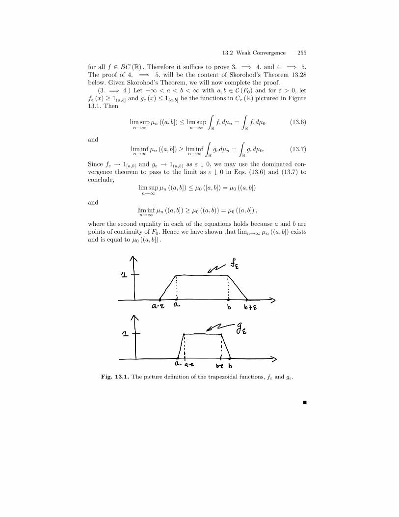
13.2 Weak Convergence 255
for all f ∈ BC (R) . Therefore it suffices to prove 3. =⇒ 4. and 4. =⇒ 5.The proof of 4. =⇒ 5. will be the content of Skorohod’s Theorem 13.28below. Given Skorohod’s Theorem, we will now complete the proof.
(3. =⇒ 4.) Let −∞ < a < b < ∞ with a, b ∈ C (F0) and for ε > 0, letfε (x) ≥ 1(a,b] and gε (x) ≤ 1(a,b] be the functions in Cc (R) pictured in Figure13.1. Then
lim supn→∞
µn ((a, b]) ≤ lim supn→∞
∫Rfεdµn =
∫Rfεdµ0 (13.6)
andlim infn→∞
µn ((a, b]) ≥ lim infn→∞
∫Rgεdµn =
∫Rgεdµ0. (13.7)
Since fε → 1[a,b] and gε → 1(a,b) as ε ↓ 0, we may use the dominated con-vergence theorem to pass to the limit as ε ↓ 0 in Eqs. (13.6) and (13.7) toconclude,
lim supn→∞
µn ((a, b]) ≤ µ0 ([a, b]) = µ0 ((a, b])
andlim infn→∞
µn ((a, b]) ≥ µ0 ((a, b)) = µ0 ((a, b]) ,
where the second equality in each of the equations holds because a and b arepoints of continuity of F0. Hence we have shown that limn→∞ µn ((a, b]) existsand is equal to µ0 ((a, b]) .
Fig. 13.1. The picture definition of the trapezoidal functions, fε and gε.

256 13 Weak Convergence Results
Corollary 13.18. Suppose that Xn∞n=0 is a sequence of random variables,
such that XnP→ X0, then Xn =⇒ X0. (Recall that example 13.16 shows the
converse is in general false.)
Proof. Let g ∈ BC (R) , then by Corollary 11.9, g (Xn) P→ g (X0) andsince g is bounded, we may apply the dominated convergence theorem (seeCorollary 11.8) to conclude that E [g (Xn)] → E [g (X0)] .
Lemma 13.19. Suppose Xn∞n=1 is a sequence of random variables on a
common probability space and c ∈ R. Then Xn =⇒ c iff XnP→ c.
Proof. Recall that XnP→ c iff for all ε > 0, P (|Xn − c| > ε) → 0. Since
|Xn − c| > ε = Xn > c+ ε ∪ Xn < c− ε
it follows XnP→ c iff P (Xn > x) → 0 for all x > c and P (Xn < x) → 0 for all
x < c. These conditions are also equivalent to P (Xn ≤ x) → 1 for all x > cand P (Xn ≤ x) ≤ P (Xn ≤ x′) → 0 for all x < c (where x < x′ < c). SoXn
P→ c iff
limn→∞
P (Xn ≤ x) =
0 if x < c1 if x > c
= F (x)
where F (x) = P (c ≤ x) = 1x≥c. Since C (F ) = R \ c , we have shown
XnP→ c iff Xn =⇒ c.
We end this section with a few more equivalent characterizations of weakconvergence. The combination of Theorem 13.17 and 13.20 is often called thePortmanteau Theorem.
Theorem 13.20 (The Portmanteau Theorem). Suppose Fn∞n=0 areproper distribution functions. By abuse of notation, we will denote µFn
(A)simply by Fn (A) for all A ∈ BR. Then the following are equivalent.
1. Fn =⇒ F0.2. lim infn→∞ Fn (U) ≥ F0 (U) for open subsets, U ⊂ R.3. lim supn→∞ Fn (C) ≤ F0 (C) for all closed subsets, C ⊂ R.4. limn→∞ Fn (A) = F0 (A) for all A ∈ BR such that F0 (∂A) = 0.
Proof. (1. =⇒ 2.) By Theorem 13.28 we may choose random variables,Yn, such that P (Yn ≤ y) = Fn (y) for all y ∈ R and n ∈ N and Yn → Y0 a.s.as n→∞. Since U is open, it follows that
1U (Y ) ≤ lim infn→∞
1U (Yn) a.s.
and so by Fatou’s lemma,
F (U) = P (Y ∈ U) = E [1U (Y )]≤ lim inf
n→∞E [1U (Yn)] = lim inf
n→∞P (Yn ∈ U) = lim inf
n→∞Fn (U) .

13.3 “Derived” Weak Convergence 257
(2. ⇐⇒ 3.) This follows from the observations: 1) C ⊂ R is closed iffU := Cc is open, 2) F (U) = 1 − F (C) , and 3) lim infn→∞ (−Fn (C)) =− lim supn→∞ Fn (C) .
(2. and 3. ⇐⇒ 4.) If F0 (∂A) = 0, then Ao ⊂ A ⊂ A with F0
(A \Ao
)=
0. Therefore
F0 (A) = F0 (Ao) ≤ lim infn→∞
Fn (Ao) ≤ lim supn→∞
Fn
(A)≤ F0
(A)
= F0 (A) .
(4. =⇒ 1.) Let a, b ∈ C (F0) and take A := (a, b]. Then F0 (∂A) =F0 (a, b) = 0 and therefore, limn→∞ Fn ((a, b]) = F0 ((a, b]) , i.e. Fn =⇒ F0.
Exercise 13.3. Suppose that F is a continuous proper distribution function.Show,
1. F : R → [0, 1] is uniformly continuous.2. If Fn∞n=1 is a sequence of distribution functions converging weakly to F,
then Fn converges to F uniformly on R, i.e.
limn→∞
supx∈R
|F (x)− Fn (x)| = 0.
In particular, it follows that
supa<b
|µF ((a, b])− µFn((a, b])| = sup
a<b|F (b)− F (a)− (Fn (b)− Fn (a))|
≤ supb|F (b)− Fn (b)|+ sup
a|Fn (a)− Fn (a)|
→ 0 as n→∞.
Hints for part 2. Given ε > 0, show that there exists, −∞ = α0 < α1 <· · · < αn = ∞, such that |F (αi+1)− F (αi)| ≤ ε for all i. Now show, forx ∈ [αi, αi+1), that
|F (x)− Fn (x)| ≤ (F (αi+1)− F (αi))+|F (αi)− Fn (αi)|+(Fn (αi+1)− Fn (αi)) .
13.3 “Derived” Weak Convergence
Lemma 13.21. Let (X, d) be a metric space, f : X → R be a function, andD (f) be the set of x ∈ X where f is discontinuous at x. Then D (f) is a Borelmeasurable subset of X.
Proof. For x ∈ X and δ > 0, let Bx (δ) = y ∈ X : d (x, y) < δ . Givenδ > 0, let fδ : X → R∪∞ be defined by,
fδ (x) := supy∈Bx(δ)
f (y) .

258 13 Weak Convergence Results
We will begin by showing fδ is lower semi-continuous, i.e.fδ ≤ a
is
closed (or equivalentlyfδ > a
is open) for all a ∈ R. Indeed, if fδ (x) > a,
then there exists y ∈ Bx (δ) such that f (y) > a. Since this y is in Bx′ (δ)whenever d (x, x′) < δ− d (x, y) (because then, d (x′, y) ≤ d (x, y)+ d (x, x′) <δ) it follows that fδ (x′) > a for all x′ ∈ Bx (δ − d (x, y)) . This shows
fδ > a
is open in X.
We similarly define fδ : X → R∪−∞ by
fδ (x) := infy∈Bx(δ)
f (y) .
Since fδ = − (−f)δ, it follows that
fδ ≥ a =
(−f)δ ≤ −a
is closed for all a ∈ R, i.e. fδ is upper semi-continuous. Moreover, fδ ≤f ≤ fδ for all δ > 0 and fδ ↓ f0 and fδ ↑ f0 as δ ↓ 0, where f0 ≤ f ≤ f0 andf0 : X → R∪−∞ and f0 : X → R∪∞ are measurable functions. Theproof is now complete since it is easy to see that
D (f) =f0 > f0
=f0 − f0 6= 0
∈ BX .
Remark 13.22. Suppose that xn → x with x ∈ C (f) := D (f)c. Then f (xn) →
f (x) as n→∞.
Theorem 13.23 (Continuous Mapping Theorem). Let f : R → R be aBorel measurable functions. If Xn =⇒ X0 and P (X0 ∈ D (f)) = 0, thenf (Xn) =⇒ f (X0) . If in addition, f is bounded, Ef (Xn) → Ef (X0) .
Proof. Let Yn∞n=0 be random variables on some probability space asin Theorem 13.28. For g ∈ BC (R) we observe that D (g f) ⊂ D (f) andtherefore,
P (Y0 ∈ D (g f)) ≤ P (Y0 ∈ D (f)) = P (X0 ∈ D (f)) = 0.
Hence it follows that g f Yn → g f Y0 a.s. So an application of thedominated convergence theorem (see Corollary 11.8) implies
E [g (f (Xn))] = E [g (f (Yn))] → E [g (f (Y0))]= E [g (f (X0))] . (13.8)
This proves the first assertion. For the second assertion we take g (x) =(x ∧M) ∨ (−M) in Eq. (13.8) where M is a bound on |f | .
Theorem 13.24 (Slutzky’s Theorem). Suppose that Xn =⇒ X andYn
P→ c where c is a constant. Then (Xn, Yn) =⇒ (X, c) in the sensethat E [f (Xn, Yn)] → E [f (X, c)] for all f ∈ BC
(R2). In particular, by tak-
ing f (x, y) = g (x+ y) and f (x, y) = g (x · y) with g ∈ BC (R) , we learnXn + Yn =⇒ X + c and Xn · Yn =⇒ X · c respectively.

13.3 “Derived” Weak Convergence 259
Proof. First suppose that f ∈ Cc
(R2), and for ε > 0, let δ := δ (ε) be
chosen so that
|f (x, y)− f (x′, y′)| ≤ ε if ‖(x, y)− (x′, y′)‖ ≤ δ.
Then
|E [f (Xn, Yn)− f (Xn, c)]| ≤ E [|f (Xn, Yn)− f (Xn, c)| : |Yn − c| ≤ δ]+ E [|f (Xn, Yn)− f (Xn, c)| : |Yn − c| > δ]≤ ε+ 2MP (|Yn − c| > δ) → ε as n→∞,
where M = sup |f | . Since, Xn =⇒ X, we know E [f (Xn, c)] → E [f (X, c)]and hence we have shown,
lim supn→∞
|E [f (Xn, Yn)− f (X, c)]|
≤ lim supn→∞
|E [f (Xn, Yn)− f (Xn, c)]|+ lim supn→∞
|E [f (Xn, c)− f (X, c)]| ≤ ε.
Since ε > 0 was arbitrary, we learn that limn→∞ Ef (Xn, Yn) = Ef (X, c) .Now suppose f ∈ BC
(R2)
with f ≥ 0 and let ϕk (x, y) ∈ [0, 1] be contin-uous functions with compact support such that ϕk (x, y) = 1 if |x| ∨ |y| ≤ kand ϕk (x, y) ↑ 1 as k → ∞. Then applying what we have just proved tofk := ϕkf, we find
E [fk (X, c)] = limn→∞
E [fk (Xn, Yn)] ≤ lim infn→∞
E [f (Xn, Yn)] .
Letting k →∞ in this inequality then implies that
E [f (X, c)] ≤ lim infn→∞
E [f (Xn, Yn)] .
This inequality with f replaced by M − f ≥ 0 then shows,
M − E [f (X, c)] ≤ lim infn→∞
E [M − f (Xn, Yn)] = M − lim supn→∞
E [f (Xn, Yn)] .
Hence we have shown,
lim supn→∞
E [f (Xn, Yn)] ≤ E [f (X, c)] ≤ lim infn→∞
E [f (Xn, Yn)]
and therefore limn→∞ E [f (Xn, Yn)] = E [f (X, c)] for all f ∈ BC(R2)
withf ≥ 0. This completes the proof since any f ∈ BC
(R2)
may be written as adifference of its positive and negative parts.
Theorem 13.25 (δ – method). Suppose that Xn∞n=1 are random vari-ables, b ∈ R, an ∈ R\ 0 with limn→∞ an = 0, and
Xn − b
an=⇒ Z.
If g : R → R be a measurable function which is differentiable at b, then
g (Xn)− g (b)an
=⇒ g′ (b)Z.

260 13 Weak Convergence Results
Proof. Observe that
Xn − b = anXn − b
an=⇒ 0 · Z = 0
so that Xn =⇒ b and hence XnP→ b. By definition of the derivative of g at
b, we haveg (x+∆) = g (b) + g′ (b)∆+ ε (∆)∆
where ε (∆) → 0 as ∆ → 0. Let Yn and Y be random variables on a fixedprobability space such that Yn
d= Xn−ban
and Yd= Z with Yn → Y a.s. Then
Xnd= anYn + b, so that
g (Xn)− g (b)an
d=g (anYn + b)− g (b)
an= g′ (b)Yn +
anYnε (anYn)an
= g′ (b)Yn + Ynε (anYn) → g′ (b)Y a.s.
This completes the proof since g′ (b)Y d= g′ (b)Z.
Example 13.26. Suppose that Un∞n=1 are i.i.d. random variables which are
uniformly distributed on [0, 1] and let Yn :=∏n
j=1 U1nj . Our goal is to find
an and bn such that Yn−bn
anis weakly convergent to a non-constant random
variable. To this end, let
Xn := lnYn =1n
n∑j=1
lnUj .
By the strong law of large numbers,
limn→∞
Xna.s.= E [lnU1] =
∫ 1
0
lnxdx = [x lnx− x]10 = −1
and therefore, limn→∞ Yna.s.= e−1.
Let us further observe that
E[ln2 U1
]=∫ 1
0
ln2 xdx = 2
so that Var (lnU1) = 2− (−1)2 = 1. Hence by the central limit theorem,
Xn − (−1)1√n
=√n (Xn + 1) =⇒ N (0, 1) .
Therefore the δ – method implies,
g (Xn)− g (−1)1√n
=⇒ g′ (−1)N (0, 1) .

13.4 Skorohod and the Convergence of Types Theorems 261
Taking g (x) := ex using g (Xn) = eXn = Yn, then implies
Yn − e−1
1√n
=⇒ e−1N (0, 1) d= N(0, e−2
).
Hence we have shown,
√n
n∏j=1
U1nj − e−1
=⇒ N(0, e−2
).
Exercise 13.4. Given a function, f : X → R and a point x ∈ X, let
lim infy→x
f (y) := limε↓0
infy∈B′x(δ)
f (y) and (13.9)
lim supy→x
f (y) := limε↓0
supy∈B′x(δ)
f (y) , (13.10)
whereB′x (δ) := y ∈ X : 0 < d (x, y) < δ .
Show f is lower (upper) semi-continuous iff lim infy→x f (y) ≥ f (x)(lim supy→x f (y) ≤ f (x)
)for all x ∈ X.
Solution to Exercise (13.4). Suppose Eq. (13.9) holds, a ∈ R, and x ∈ Xsuch that f (x) > a. Since,
limε↓0
infy∈B′x(δ)
f (y) = lim infy→x
f (y) ≥ f (x) > a,
it follows that infy∈B′x(δ) f (y) > a for some δ > 0. Hence we may concludethat Bx (δ) ⊂ f > a which shows f > a is open.
Conversely, suppose now that f > a is open for all a ∈ R. Given x ∈X and a < f (x) , there exists δ > 0 such that Bx (δ) ⊂ f > a . Henceit follows that lim infy→x f (y) ≥ a and then letting a ↑ f (x) then implieslim infy→x f (y) ≥ f (x) .
13.4 Skorohod and the Convergence of Types Theorems
Notation 13.27 Given a proper distribution function, F : R → [0, 1] , let Y =F← : (0, 1) → R be the function defined by
Y (x) = F← (x) = sup y ∈ R : F (y) < x .
Similarly, letY + (x) := inf y ∈ R : F (y) > x .
We will need the following simple observations about Y and Y + which areeasily understood from Figure 13.4.

262 13 Weak Convergence Results
1. Y (x) ≤ Y + (x) and Y (x) < Y + (x) iff x is the height of a “flat spot” ofF.
2. The set, E := x ∈ (0, 1) : Y (x) < Y + (x) , of flat spot heights is at mostcountable. This is because, (Y (x) , Y + (x))x∈E is a collection of pair-wise disjoint intervals which is necessarily countable. (Each such intervalcontains a rational number.)
3. The following inequality holds,
F (Y (x)−) ≤ x ≤ F (Y (x)) for all x ∈ (0, 1) . (13.11)
Indeed, if y > Y (x) , then F (y) ≥ x and by right continuity of F itfollows that F (Y (x)) ≥ x. Similarly, if y < Y (x) , then F (y) < x andhence F (Y (x)−) ≤ x.
4. x ∈ (0, 1) : Y (x) ≤ y0 = (0, F (y0)]∩ (0, 1) . To prove this assertion firstsuppose that Y (x) ≤ y0, then according to Eq. (13.11) we have x ≤F (Y (x)) ≤ F (y0) , i.e. x ∈ (0, F (y0)] ∩ (0, 1) . Conversely, if x ∈ (0, 1)and x ≤ F (y0) , then Y (x) ≤ y0 by definition of Y.
5. As a consequence of item 4. we see that Y is B(0,1)/BR – measurable andm Y −1 = F, where m is Lebesgue measure on
((0, 1) ,B(0,1)
).
Theorem 13.28 (Baby Skorohod Theorem). Suppose that Fn∞n=0 is acollection of distribution functions such that Fn =⇒ F0. Then there ex-ists a probability space, (Ω,B, P ) and random variables, Yn∞n=1 such thatP (Yn ≤ y) = Fn (y) for all n ∈ N∪∞ and limn→∞ F←n = limn→∞ Yn =Y = F← a.s.
Proof. We will take Ω := (0, 1) , B = B(0,1), and P = m – Lebesguemeasure on Ω and let Yn := F←n and Y := F←0 as in Notation 13.27. Becauseof the above comments, P (Yn ≤ y) = Fn (y) and P (Y ≤ y) = F0 (y) for ally ∈ R. So in order to finish the proof it suffices to show, Yn (x) → Y (x)for all x /∈ E, where E is the countable null set defined as above, E :=x ∈ (0, 1) : Y (x) < Y + (x) .

13.4 Skorohod and the Convergence of Types Theorems 263
We now suppose x /∈ E. If y ∈ C (F0) with y < Y (x) , we havelimn→∞ Fn (y) = F0 (y) < x and in particular, Fn (y) < x for almost all n.This implies that Yn (x) ≥ y for a.a. n and hence that lim infn→∞ Yn (x) ≥ y.Letting y ↑ Y (x) with y ∈ C (F0) then implies
lim infn→∞
Yn (x) ≥ Y (x) .
Similarly, for x /∈ E and y ∈ C (F0) with Y (x) = Y + (x) < y, we havelimn→∞ Fn (y) = F0 (y) > x and in particular, Fn (y) > x for almost all n.This implies that Yn (x) ≤ y for a.a. n and hence that lim supn→∞ Yn (x) ≤ y.Letting y ↓ Y (x) with y ∈ C (F0) then implies
lim supn→∞
Yn (x) ≤ Y (x) .
Hence we have shown, for x /∈ E, that
lim supn→∞
Yn (x) ≤ Y (x) ≤ lim infn→∞
Yn (x)
which shows
limn→∞
F←n (x) = limn→∞
Yn (x) = Y (x) = F← (x) for all x /∈ E. (13.12)
Definition 13.29. Two random variables, Y and Z, are said to be of thesame type if there exists constants, A > 0 and B ∈ R such that
Zd= AY +B. (13.13)
Alternatively put, if U (y) := P (Y ≤ y) and V (y) := P (Z ≤ y) , then U andV should satisfy,
U (y) = P (Y ≤ y) = P (Z ≤ Ay +B) = V (Ay +B) .
For the next theorem we will need the following elementary observation.
Lemma 13.30. If Y is non-constant (a.s.) random variable and U (y) :=P (Y ≤ y) , then U← (γ1) < U← (γ2) for all γ1 sufficiently close to 0 and γ2
sufficiently close to 1.
Proof. Observe that Y is constant iff U (y) = 1y≥c for some c ∈ R, i.e.iff U only takes on the values, 0, 1 . So since Y is not constant, there existsy ∈ R such that 0 < U (y) < 1. Hence if γ2 > U (y) then U← (γ2) ≥ y andif γ1 < U (y) then U← (γ1) ≤ y. Moreover, if we suppose that γ1 is not theheight of a flat spot of U, then in fact, U← (γ1) < U← (γ2) . This inequalitythen remains valid as γ1 decreases and γ2 increases.

264 13 Weak Convergence Results
Theorem 13.31 (Convergence of Types). Suppose Xn∞n=1 is a sequenceof random variables and an, αn ∈ (0,∞) , bn, βn ∈ R are constants and Y andZ are non-constant random variables. Then
1. ifXn − bnan
=⇒ Y (13.14)
andXn − βn
αn=⇒ Z, (13.15)
then Y and Z are of the same type. Moreover, the limits,
A = limn→∞
αn
an∈ (0,∞) and B := lim
n→∞
βn − bnan
(13.16)
exists and Y d= AZ +B.2. If the relations in Eq. (13.16) hold then either of the convergences in Eqs.
(13.14) or (13.15) implies the others with Z and Y related by Eq. (13.13).3. If there are some constants, an > 0 and bn ∈ R and a non-constant
random variable Y, such that Eq. (13.14) holds, then Eq. (13.15) holdsusing αn and βn of the form,
αn := F←n (γ2)− F←n (γ1) and βn := F←n (γ1) (13.17)
for some 0 < γ1 < γ2 < 1. If the Fn are invertible functions, Eq. (13.17)may be written as
Fn (βn) = γ1 and Fn (αn + βn) = γ2. (13.18)
Proof. (2) Assume the limits in Eq. (13.16) hold. If Eq. (13.14) is satisfied,then by Slutsky’s Theorem 13.20,
Xn − βn
αn=Xn − bn + bn − βn
an
an
αn
=Xn − bnan
an
αn− βn − bn
an
an
αn
=⇒ A−1 (Y −B) =: Z
Similarly, if Eq. (13.15) is satisfied, then
Xn − bnan
=Xn − βn
αn
αn
an+βn − bnan
=⇒ AZ +B =: Y.
(1) If Fn (y) := P (Xn ≤ y) , then
P
(Xn − bnan
≤ y
)= Fn (any + bn) and P
(Xn − βn
αn≤ y
)= Fn (αny + βn) .

13.4 Skorohod and the Convergence of Types Theorems 265
By assumption we have
Fn (any + bn) =⇒ U (y) and Fn (αny + βn) =⇒ V (y) .
If w := sup y : Fn (any + bn) < x , then anw + bn = F←n (x) and hence
sup y : Fn (any + bn) < x =F←n (x)− bn
an.
Similarly,
sup y : Fn (αny + βn) < x =F←n (x)− βn
αn.
With these identities, it now follows from the proof of Skorohod’s Theorem13.28 (see Eq. (13.12)) that there exists an at most countable subset, Λ, of(0, 1) such that,
F←n (x)− bnan
= sup y : Fn (any + bn) < x → U← (x) and
F←n (x)− βn
αn= sup y : Fn (αny + βn) < x → V← (x)
for all x /∈ Λ. Since Y and Z are not constants a.s., we can choose, by Lemma13.30, γ1 < γ2 not in Λ such that U← (γ1) < U← (γ2) and V← (γ1) < V← (γ2) .In particular it follows that
F←n (γ2)− F←n (γ1)an
=F←n (γ2)− bn
an− F←n (γ1)− bn
an
→ U← (γ2)− U← (γ1) > 0 (13.19)
and similarly
F←n (γ2)− F←n (γ1)αn
→ V← (γ2)− V← (γ1) > 0.
Taking ratios of the last two displayed equations shows,
αn
an→ A :=
U← (γ2)− U← (γ1)V← (γ2)− V← (γ1)
∈ (0,∞) .
Moreover,
F←n (γ1)− bnan
→ U← (γ1) and (13.20)
F←n (γ1)− βn
an=F←n (γ1)− βn
αn
αn
an→ AV← (γ1)
and therefore,

266 13 Weak Convergence Results
βn − bnan
=F←n (γ1)− βn
an− F←n (γ1)− bn
an→ AV← (γ1)− U← (γ1) := B.
(3) Now suppose that we define αn := F←n (γ2) − F←n (γ1) and βn :=F←n (γ1) , then according to Eqs. (13.19) and (13.20)we have
αn/an → U← (γ2)− U← (γ1) ∈ (0, 1) andβn − bnan
→ U← (γ1) as n→∞.
Thus we may always center and scale the Xn using αn and βn of the formdescribed in Eq. (13.17).
13.5 Weak Convergence Examples
Example 13.32. Suppose that Xn∞n=1 are i.i.d. exp (λ) – random variables,i.e. Xn ≥ 0 a.s. and P (Xn ≥ x) = e−λx for all x ≥ 0. In this case
F (x) := P (X1 ≤ x) = 1− e−λ(x∨0)
Consider Mn := max (X1, . . . , Xn) . We have, for x ≥ 0 and cn ∈ (0,∞) that
Fn (x) := P (Mn ≤ x) = P(∩n
j=1 Xj ≤ x)
=n∏
j=1
P (Xj ≤ x) = [F (x)]n =(1− e−λx
)n.
We now wish to find an > 0 and bn ∈ R such that Mn−bn
an=⇒ Y.
1. To this end we note that
P
(Mn − bn
an≤ x
)= P (Mn ≤ anx+ bn)
= Fn (anx+ bn) = [F (anx+ bn)]n .
If we demand (c.f. Eq. (13.18) above)
P
(Mn − bn
an≤ 0)
= Fn (bn) = [F (bn)]n → γ1 ∈ (0, 1) ,
then bn →∞ and we find
ln γ1 ∼ n lnF (bn) = n ln(1− e−λbn
)∼ −ne−λbn .
From this it follows that bn ∼ λ−1 lnn. Given this, we now try to find an byrequiring,
P
(Mn − bn
an≤ 1)
= Fn (an + bn) = [F (an + bn)]n → γ2 ∈ (0, 1) .

13.5 Weak Convergence Examples 267
However, by what we have done above, this requires an +bn ∼ λ−1 lnn. Hencewe may as well take an to be constant and for simplicity we take an = 1.
2. We now compute
limn→∞
P(Mn − λ−1 lnn ≤ x
)= lim
n→∞
(1− e−λ(x+λ−1 ln n)
)n
= limn→∞
(1− e−λx
n
)n
= exp(−e−λx
).
Notice that F (x) is a distribution function for some random variable, Y, andtherefore we have shown
Mn −1λ
lnn =⇒ Y as n→∞
where P (Y ≤ x) = exp(−e−λx
).
Example 13.33. For p ∈ (0, 1) , let Xp denote the number of trials to getsuccess in a sequence of independent trials with success probability p. ThenP (Xp > n) = (1− p)n and therefore for x > 0,
P (pXp > x) = P
(Xp >
x
p
)= (1− p)[
xp ] = e[
xp ] ln(1−p)
∼ e−p[ xp ] → e−x as p→ 0.
Therefore pXp =⇒ T where T d= exp (1) , i.e. P (T > x) = e−x for x ≥ 0 oralternatively, P (T ≤ y) = 1− e−y∨0.
Remarks on this example. Let us see in a couple of ways where theappropriate centering and scaling of the Xp come from in this example. Forthis let q = 1 − p, then P (Xp = n) = (1− p)n−1
p = qn−1p for n ∈ N. Alsolet
Fp (x) = P (Xp ≤ x) = P (Xp ≤ [x]) = 1− q[x]
where [x] :=∑∞
n=1 n · 1[n,n+1).Method 1. Our goal is to choose ap > 0 and bp ∈ R such that
limp ↓0 Fp (apx+ bp) exists. As above, we first demand (taking x = 0) that
limp ↓0
Fp (bp) = γ1 ∈ (0, 1) .
Since, γ1 ∼ Fp (bp) ∼ 1− qbp we require, qbp ∼ 1− γ1 and hence, c ∼ bp ln q =bp ln (1− p) ∼ −bpp. This suggests that we take bp = 1/p say. Having donethis, we would like to choose ap such that
F0 (x) := limp ↓0
Fp (apx+ bp) exists.
Since,
268 13 Weak Convergence Results
F0 (x) ∼ Fp (apx+ bp) ∼ 1− qapx+bp
this requires that
(1− p)apx+bp = qapx+bp ∼ 1− F0 (x)
and hence that
ln (1− F0 (x)) = (apx+ bp) ln q ∼ (apx+ bp) (−p) = −papx− 1.
From this (setting x = 1) we see that pap ∼ c > 0. Hence we might takeap = 1/p as well. We then have
Fp (apx+ bp) = Fp
(p−1x+ p−1
)= 1− (1− p)[p
−1(x+1)]
which is equal to 0 if x ≤ −1, and for x > −1 we find
(1− p)[p−1(x+1)] = exp
([p−1 (x+ 1)
]ln (1− p)
)→ exp (− (x+ 1)) .
Hence we have shown,
limp ↓0
Fp (apx+ bp) = [1− exp (− (x+ 1))] 1x≥−1
Xp − 1/p1/p
= pXp − 1 =⇒ T − 1
or again that pXp =⇒ T.Method 2. (Center and scale using the first moment and the variance of
Xp.) The generating function is given by
f (z) := E[zXp
]=∞∑
n=1
znqn−1p =pz
1− qz.
Observe that f (z) is well defined for |z| < 1q and that f (1) = 1, reflecting the
fact that P (Xp ∈ N) = 1, i.e. a success must occur almost surely. Moreover,we have
f ′ (z) = E[Xpz
Xp−1], f ′′ (z) = E
[Xp (Xp − 1) zXp−2
], . . .
f (k) (z) = E[Xp (Xp − 1) . . . (Xp − k + 1) zXp−k
]and in particular,
E [Xp (Xp − 1) . . . (Xp − k + 1)] = f (k) (1) =(d
dz
)k
|z=1pz
1− qz.
Sinced
dz
pz
1− qz=p (1− qz) + qpz
(1− qz)2=
p
(1− qz)2
13.5 Weak Convergence Examples 269
andd2
dz2
pz
1− qz= 2
pq
(1− qz)3
it follows that
µp := EXp =p
(1− q)2=
1p
and
E [Xp (Xp − 1)] = 2pq
(1− q)3=
2qp2.
Therefore,
σ2p = Var (Xp) = EX2
p − (EXp)2 =
2qp2
+1p−(
1p
)2
=2q + p− 1
p2=
q
p2=
1− p
p2.
Thus, if we had used µp and σp to center and scale Xp we would have consid-ered,
Xp − 1p
√1−pp
=pXp − 1√
1− p=⇒ T − 1
instead.
Theorem 13.34. Let Xn∞n=1 be i.i.d. random variables such that P (Xn = ±1) =1/2 and let Sn := X1 + · · ·+Xn – the position of a drunk after n steps. Ob-serve that |Sn| is an odd integer if n is odd and an even integer if n is even.Then Sm√
m=⇒ N (0, 1) as m→∞.
Proof. (Sketch of the proof.) We start by observing that S2n = 2k iff
# i ≤ 2n : Xi = 1 = n+ k while# i ≤ 2n : Xi = −1 = 2n− (n+ k) = n− k
and therefore,
P (S2n = 2k) =(
2nn+ k
)(12
)2n
=(2n)!
(n+ k)! · (n− k)!
(12
)2n
.
Recall Stirling’s formula states,
n! ∼ nne−n√
2πn as n→∞
and therefore,

270 13 Weak Convergence Results
P (S2n = 2k)
∼ (2n)2ne−2n
√4πn
(n+ k)n+ke−(n+k)
√2π (n+ k) · (n− k)n−k
e−(n−k)√
2π (n− k)
(12
)2n
=√
n
π (n+ k) (n− k)
(1 +
k
n
)−(n+k)
·(
1− k
n
)−(n−k)
=1√πn
√1(
1 + kn
) (1− k
n
) (1− k2
n2
)−n
·(
1 +k
n
)−k
·(
1− k
n
)k
=1√πn
(1− k2
n2
)−n
·(
1 +k
n
)−k−1/2
·(
1− k
n
)k−1/2
.
So if we let x := 2k/√
2n, i.e. k = x√n/2 and k/n = x√
2n, we have
P
(S2n√2n
= x
)
∼ 1√πn
(1− x2
2n
)−n
·(
1 +x√2n
)−x√
n/2−1/2
·(
1− x√2n
)x√
n/2−1/2
∼ 1√πn
ex2/2 · ex√2n
−x√
n/2−1/2· e−
x√2n
x√
n/2−1/2
∼ 1√πn
e−x2/2,
wherein we have repeatedly used
(1 + an)bn = ebn ln(1+an) ∼ ebnan when an → 0.
We now compute
P
(a ≤ S2n√
2n≤ b
)=∑
a≤x≤b
P
(S2n√2n
= x
)=
1√2π
∑a≤x≤b
e−x2/2 2√2n
(13.21)
where the sum is over x of the form, x = 2k√2n
with k ∈ 0,±1, . . . ,±n . Since2√2n
is the increment of x as k increases by 1, we see the latter expression inEq. (13.21) is the Riemann sum approximation to
1√2π
∫ b
a
e−x2/2dx.
This proves S2n√2n
=⇒ N (0, 1) . Since

13.5 Weak Convergence Examples 271
S2n+1√2n+ 1
=S2n +X2n+1√
2n+ 1=
S2n√2n
1√1 + 1
2n
+X2n+1√2n+ 1
,
it follows directly (or see Slutsky’s Theorem 13.20) that S2n+1√2n+1
=⇒ N (0, 1)as well.
Proposition 13.35. Suppose that Un∞n=1 are i.i.d. random variables whichare uniformly distributed in (0, 1) . Let U(k,n) denote the position of the kth –largest number from the list, U1, U2, . . . , Un . Further let k (n) be chosen sothat limn→∞ k (n) = ∞ while limn→∞
k(n)n = 0 and let
Xn :=U(k(n),n) − k (n) /n
√k(n)
n
.
Then dTV (Xn, N (0, 1)) → 0 as n→∞.
Proof. (Sketch only. See Resnick, Proposition 8.2.1 for more details.) Ob-serve that, for x ∈ (0, 1) , that
P(U(k,n) ≤ x
)= P
(n∑
i=1
Xi ≥ k
)=
n∑l=k
(n
l
)xl (1− x)n−l
.
From this it follows that ρn (x) := 1(0,1) (x) ddxP
(U(k,n) ≤ x
)is the probability
density for U(k,n). It now turns out that ρn (x) is a Beta distribution,
ρn (x) =(n
k
)k · xk−1 (1− x)n−k
.
Giving a direct computation of this result is not so illuminating. So let us goanother route. To do this we are going to estimate, P
(U(k,n) ∈ (x, x+∆]
),
for ∆ ∈ (0, 1) . Observe that if U(k,n) ∈ (x, x+∆], then there must be at leastone Ui ∈ (x, x+∆], for otherwise, U(k,n) ≤ x+∆ would imply U(k,n) ≤ x aswell and hence U(k,n) /∈ (x, x+∆]. Let
Ωi := Ui ∈ (x, x+∆] and Uj /∈ (x, x+∆] for j 6= i .
Since
P (Ui, Uj ∈ (x, x+∆] for some i 6= j with i, j ≤ n) ≤∑
i<j≤n
P (Ui, Uj ∈ (x, x+∆])
≤ n2 − n
2∆2,
we see that
272 13 Weak Convergence Results
P(U(k,n) ∈ (x, x+∆]
)=
n∑i=1
P(U(k,n) ∈ (x, x+∆], Ωi
)+O
(∆2)
= nP(U(k,n) ∈ (x, x+∆], Ω1
)+O
(∆2).
Now on the set, Ω1; U(k,n) ∈ (x, x+∆] iff there are exactly k−1 of U2, . . . , Un
in [0, x] and n− k of these in [x+∆, 1] . This leads to the conclusion that
P(U(k,n) ∈ (x, x+∆]
)= n
(n− 1k − 1
)xk−1 (1− (x+∆))n−k
∆+O(∆2)
and therefore,
ρn (x) = lim∆↓0
P(U(k,n) ∈ (x, x+∆]
)∆
=n!
(k − 1)! · (n− k)!xk−1 (1− x)n−k
.
By Stirling’s formula,
n!(k − 1)! · (n− k)!
∼ nne−n√
2πn
(k − 1)(k−1)e−(k−1)
√2π (k − 1) (n− k)(n−k)
e−(n−k)√
2π (n− k)
=√ne−1
√2π
1(k−1
n
)(k−1)√
k−1n
(n−k
n
)(n−k)√
n−kn
=√ne−1
√2π
1(k−1
n
)(k−1/2) (1− k
n
)(n−k+1/2).
Since (k − 1n
)(k−1/2)
=(k
n
)(k−1/2)
·(k − 1k
)(k−1/2)
=(k
n
)(k−1/2)
·(
1− 1k
)(k−1/2)
∼ e−1
(k
n
)(k−1/2)
we arrive at
n!(k − 1)! · (n− k)!
∼√n√2π
1(kn
)(k−1/2) (1− k
n
)(n−k+1/2).
By the change of variables formula, with
x =u− k (n) /n√
k(n)
n

13.6 Compactness and Tightness 273
on noting the du =√
k(n)
n dx, x = −√k (n) at u = 0, and
x =1− k (n) /n√
k(n)
n
=n− k (n)√
k (n)
=n√k (n)
(1− k (n)
n
)=√n
√n
k (n)
(1− k (n)
n
)=: bn,
E [F (Xn)] =∫ 1
0
ρn (u)F
u− k (n) /n√k(n)
n
du
=∫ bn
−√
k(n)
√k (n)n
ρn
(√k (n)n
x+ k (n) /n
)F (x) du.
Using this information, it is then shown in Resnick that√k (n)n
ρn
(√k (n)n
x+ k (n) /n
)→ e−x2/2
√2π
which upon an application of Scheffe’s Lemma 13.3 completes the proof.
Remark 13.36. It is possible to understand the normalization constants in thedefinition of Xn by computing the mean and the variance of U(n,k). Aftersome computations (see Chapter ??), one arrives at
EU(k,n) =∫ 1
0
n!(k − 1)! · (n− k)!
xk−1 (1− x)n−kxdx
=k
n+ 1∼ k
n,
EU2(k,n) =
∫ 1
0
n!(k − 1)! · (n− k)!
xk−1 (1− x)n−kx2dx
=(k + 1) k
(n+ 2) (n+ 1)and
Var(U(k,n)
)=
(k + 1) k(n+ 2) (n+ 1)
− k2
(n+ 1)2
=k
n+ 1
[k + 1n+ 2
− k
n+ 1
]=
k
n+ 1
[n− k + 1
(n+ 2) (n+ 1)
]∼ k
n2.
13.6 Compactness and Tightness
Suppose that Λ ⊂ R is a dense set and F and F are two right continuousfunctions. If F = F on Λ, then F = F on R. Indeed, for x ∈ R we have

274 13 Weak Convergence Results
F (x) = limΛ3λ↓x
F (λ) = limΛ3λ↓x
F (λ) = F (x) .
Lemma 13.37. If G : Λ→ R is a non-decreasing function, then
F (x) := G (x+) := limΛ3λ↓x
G (λ) (13.22)
is a non-decreasing right continuous function.
Proof. To show F is right continuous, let x, y ∈ R with x < y and letλ ∈ Λ such that x < y < λ. Then
F (x) ≤ F (y) = G (y+) ≤ G (λ)
and therefore,F (x) ≤ F (x+) := lim
y↓xF (y) ≤ G (λ) .
Since λ > x with λ ∈ Λ is arbitrary, we may conclude, F (x) ≤ F (x+) ≤G (x+) = F (x) , i.e. F (x+) = F (x) .
Proposition 13.38. Suppose that Fn∞n=1 is a sequence of distribution func-tions and Λ ⊂ R is a dense set such that G (λ) := limn→∞ Fn (λ) ∈ [0, 1]exists for all λ ∈ Λ. If, for all x ∈ R, we define F as in Eq. (13.22), thenFn (x) → F (x) for all x ∈ C (F ) . (Note well; as we have already seen, it ispossible that F (∞) < 1 and F (−∞) > 0 so that F need not be a distributionfunction for a measure on (R,BR) .)
Proof. Suppose that x, y ∈ R with x < y and and s, t ∈ Λ are chosen sothat x < s < y < t. Then passing to the limit in the inequality,
Fn (s) ≤ Fn (y) ≤ Fn (t)
implies
F (x) = G (x+) ≤ G (s) ≤ lim infn→∞
Fn (y) ≤ lim supn→∞
Fn (y) ≤ G (t) .
Then letting t ∈ Λ tend down to y and then let x ∈ R tend up to y, we mayconclude
F (y−) ≤ lim infn→∞
Fn (y) ≤ lim supn→∞
Fn (y) ≤ F (y) for all y ∈ R.
This completes the proof, since F (y−) = F (y) for y ∈ C (F ) .The next theorem deals with weak convergence of measures on
(R,BR
).
So as not have to introduce any new machinery, the reader should identify Rwith [−1, 1] ⊂ R via the map,
[−1, 1] 3 x→ tan(π
2x)∈ R.
13.6 Compactness and Tightness 275
Hence a probability measure on(R,BR
)may be identified with a probability
measure on (R,BR) which is supported on [−1, 1] . Using this identification, wesee that a −∞ should only be considered a point of continuity of a distributionfunction, F : R → [0, 1] iff and only if F (−∞) = 0. On the other hand, ∞ isalways a point of continuity.
Theorem 13.39 (Helly’s Selection Theorem). Every sequence of prob-ability measures, µn∞n=1 , on
(R,BR
)has a sub-sequence which is weakly
convergent to a probability measure, µ0 on(R,BR
).
Proof. Using the identification described above, rather than viewing µn asprobability measures on
(R,BR
), we may view them as probability measures
on (R,BR) which are supported on [−1, 1] , i.e. µn ([−1, 1]) = 1. As usual, let
Fn (x) := µn ((−∞, x]) = µn ((−∞, x] ∩ [−1, 1]) .
Since Fn (x)∞n=1 ⊂ [0, 1] and [0, 1] is compact, for each x ∈ R we may find aconvergence subsequence of Fn (x)∞n=1 . Hence by Cantor’s diagonalizationargument we may find a subsequence, Gk := Fnk
∞k=1 of the Fn∞n=1 suchthat G (x) := limk→∞Gk (x) exists for all x ∈ Λ := Q.
Letting F (x) := G (x+) as in Eq. (13.22), it follows from Lemma 13.37and Proposition 13.38 that Gk = Fnk
=⇒ F0. Moreover, since Gk (x) = 0for all x ∈ Q∩ (−∞,−1) and Gk (x) = 1 for all x ∈ Q ∩ [1,∞). Therefore,F0 (x) = 1 for all x ≥ 1 and F0 (x) = 0 for all x < −1 and the correspondingmeasure, µ0 is supported on [−1, 1] . Hence µ0 may now be transferred backto a measure on
(R,BR
).
Example 13.40. Suppose δ−n =⇒ δ−∞ and δn =⇒ δ∞ and12 (δn + δ−n) =⇒ 1
2 (δ∞ + δ−∞) . This shows that probability may indeedtransfer to the points at ±∞.
The next question we would like to address is when is the limiting measure,µ0 on
(R,BR
)concentrated on R. The following notion of tightness is the key
to answering this question.
Definition 13.41. A collection of probability measures, Γ, on (R,BR) is tightiff for every ε > 0 there exists Mε <∞ such that
infµ∈Γ
µ ([−Mε,Mε]) ≥ 1− ε. (13.23)
We further say that a collection of random variables, Xλ : λ ∈ Λ is tight iffthe collection probability measures,
P X−1
λ : λ ∈ Λ
is tight. Equivalentlyput, Xλ : λ ∈ Λ is tight iff
limM→∞
supλ∈Λ
P (|Xλ| ≥M) = 0. (13.24)

276 13 Weak Convergence Results
Observe that the definition of uniform integrability (see Definition 11.25)is considerably stronger than the notion of tightness. It is also worth observingthat if α > 0 and C := supλ∈Λ E |Xλ|α <∞, then by Chebyschev’s inequality,
supλP (|Xλ| ≥M) ≤ sup
λ
[1Mα
E |Xλ|α]≤ C
Mα→ 0 as M →∞
and therefore Xλ : λ ∈ Λ is tight.
Theorem 13.42. Let Γ := µn∞n=1 be a sequence of probability measures on(R,BR) . Then Γ is tight, iff every subsequently limit measure, µ0, on
(R,BR
)is supported on R. In particular if Γ is tight, there is a weakly convergentsubsequence of Γ converging to a probability measure on (R,BR) .
Proof. Suppose that µnk=⇒ µ0 with µ0 being a probability measure on(
R,BR). As usual, let F0 (x) := µ0 ([−∞, x]) . If Γ is tight and ε > 0 is given,
we may find Mε <∞ such that Mε,−Mε ∈ C (F0) and µn ([−Mε,Mε]) ≥ 1−εfor all n. Hence it follows that
µ0 ([−Mε,Mε]) = limk→∞
µnk([−Mε,Mε]) ≥ 1− ε
and by letting ε ↓ 0 we conclude that µ0 (R) = limε↓0 µ0 ([−Mε,Mε]) = 1.Conversely, suppose there is a subsequence µnk
∞k=1 such that µnk=⇒
µ0 with µ0 being a probability measure on(R,BR
)such that µ0 (R) < 1. In
this case ε0 := µ0 (−∞,∞) > 0 and hence for all M <∞ we have
µ0 ([−M,M ]) ≤ µ0
(R)− µ0 (−∞,∞) = 1− ε0.
By choosing M so that −M and M are points of continuity of F0, it thenfollows that
limk→∞
µnk([−M,M ]) = µ0 ([−M,M ]) ≤ 1− ε0.
Therefore,infn∈N
µn (([−M,M ])) ≤ 1− ε0 for all M <∞
and µn∞n=1 is not tight.
13.7 Weak Convergence in Metric Spaces
(This section may be skipped.)Definition 13.43. Let X be a metric space. A sequence of probability mea-sures Pn∞n=1 is said to converge weakly to a probability P if limn→∞ Pn(f) =P (f) for all for every f ∈ BC(X). This is actually weak-* convergence whenviewing Pn ∈ BC(X)∗.
13.7 Weak Convergence in Metric Spaces 277
For simplicity we will now assume that X is a complete metric spacethroughout this section.
Proposition 13.44. The following are equivalent:
1. Pnw→ P as n→∞, i.e. Pn (f) → P (f) for all f ∈∈ BC(X).
2. Pn(f) → P (f) for every f ∈ BC(X) which is uniformly continuous.3. lim sup
n→∞Pn(F ) ≤ P (F ) for all F @ X.
4. lim infn→∞ Pn(G) ≥ P (G) for all G ⊂o X.5. limn→∞ Pn(A) = P (A) for all A ∈ B such that P (bd(A)) = 0.
Proof. 1. =⇒ 2. is obvious. For 2. =⇒ 3., let
ϕ(t) :=
1 if t ≤ 01− t if 0 ≤ t ≤ 1
0 if t ≥ 1(13.25)
and let fn(x) := ϕ(nd(x, F )). Then fn ∈ BC(X, [0, 1]) is uniformly continu-ous, 0 ≤ 1F ≤ fn for all n and fn ↓ 1F as n→∞. Passing to the limit n→∞in the equation
0 ≤ Pn(F ) ≤ Pn(fm)
gives0 ≤ lim sup
n→∞Pn(F ) ≤ P (fm)
and then lettingm→∞ in this inequality implies item 3. 3. ⇐⇒ 4. Assumingitem 3., let F = Gc, then
1− lim infn→∞
Pn(G) = lim supn→∞
(1− Pn(G)) = lim supn→∞
Pn(Gc)
≤ P (Gc) = 1− P (G)
which implies 4. Similarly 4. =⇒ 3. 3. ⇐⇒ 5. Recall that bd(A) = A \Ao,so if P (bd(A)) = 0 and 3. (and hence also 4. holds) we have
lim supn→∞
Pn(A) ≤ lim supn→∞
Pn(A) ≤ P (A) = P (A) and
lim infn→∞
Pn(A) ≥ lim infn→∞
Pn(Ao) ≥ P (Ao) = P (A)
from which it follows that limn→∞ Pn(A) = P (A). Conversely, let F @ X andset Fδ := x ∈ X : ρ(x, F ) ≤ δ . Then
bd(Fδ) ⊂ Fδ \ x ∈ X : ρ(x, F ) < δ = Aδ
where Aδ := x ∈ X : ρ(x, F ) = δ . Since Aδδ>0 are all disjoint, we musthave ∑
δ>0
P (Aδ) ≤ P (X) ≤ 1

278 13 Weak Convergence Results
and in particular the set Λ := δ > 0 : P (Aδ) > 0 is at most countable. Letδn /∈ Λ be chosen so that δn ↓ 0 as n→∞, then
P (Fδm) = lim
n→∞Pn(Fδm
) ≥ lim supn→∞
Pn(F ).
Let m → ∞ in this equation to conclude P (F ) ≥ lim supn→∞ Pn(F ) as de-sired. To finish the proof we will now show 3. =⇒ 1. By an affine change ofvariables it suffices to consider f ∈ C(X, (0, 1)) in which case we have
k∑i=1
(i− 1)k
1 (i−1)k ≤f< i
k ≤ f ≤k∑
i=1
i
k1 (i−1)
k ≤f< ik. (13.26)
Let Fi :=
ik ≤ f
and notice that Fk = ∅. Then for any probability P,
k∑i=1
(i− 1)k
[P (Fi−1)− P (Fi)] ≤ P (f) ≤k∑
i=1
i
k[P (Fi−1)− P (Fi)] . (13.27)
Since
k∑i=1
(i− 1)k
[P (Fi−1)− P (Fi)]
=k∑
i=1
(i− 1)k
P (Fi−1)−k∑
i=1
(i− 1)k
P (Fi)
=k−1∑i=1
i
kP (Fi)−
k∑i=1
i− 1k
P (Fi) =1k
k−1∑i=1
P (Fi)
and
k∑i=1
i
k[P (Fi−1)− P (Fi)]
=k∑
i=1
i− 1k
[P (Fi−1)− P (Fi)] +k∑
i=1
1k
[P (Fi−1)− P (Fi)]
=k−1∑i=1
P (Fi) +1k,
Eq. (13.27) becomes,
1k
k−1∑i=1
P (Fi) ≤ P (f) ≤ 1k
k−1∑i=1
P (Fi) + 1/k.
Using this equation with P = Pn and then with P = P we find

13.7 Weak Convergence in Metric Spaces 279
lim supn→∞
Pn(f) ≤ lim supn→∞
[1k
k−1∑i=1
Pn(Fi) + 1/k
]
≤ 1k
k−1∑i=1
P (Fi) + 1/k ≤ P (f) + 1/k.
Since k is arbitrary, lim supn→∞ Pn(f) ≤ P (f). Replacing f by 1 − f inthis inequality also gives lim infn→∞ Pn(f) ≥ P (f) and hence we have shownlimn→∞ Pn(f) = P (f) as claimed.
Theorem 13.45 (Skorohod Theorem). Let (X, d) be a separable metricspace and µn∞n=0 be probability measures on (X,BX) such that µn =⇒ µ0
as n → ∞. Then there exists a probability space, (Ω,B, P ) and measurablefunctions, Yn : Ω → X, such that µn = P Y −1
n for all n ∈ N0 := N∪0 andlimn→∞ Yn = Y a.s.
Proof. See Theorem 4.30 on page 79 of Kallenberg [3].
Definition 13.46. Let X be a topological space. A collection of probabilitymeasures Λ on (X,BX) is said to be tight if for every ε > 0 there exists acompact set Kε ∈ BX such that P (Kε) ≥ 1− ε for all P ∈ Λ.
Theorem 13.47. Suppose X is a separable metrizable space and Λ =Pn∞n=1 is a tight sequence of probability measures on BX . Then there existsa subsequence Pnk
∞k=1 which is weakly convergent to a probability measureP on BX .
Proof. First suppose that X is compact. In this case C(X) is a Banachspace which is separable by the Stone – Weirstrass theorem, see Exercise ??.By the Riesz theorem, Corollary ??, we know that C(X)∗ is in one to onecorrespondence with the complex measures on (X,BX). We have also seenthat C(X)∗ is metrizable and the unit ball in C(X)∗ is weak - * compact,see Theorem ??. Hence there exists a subsequence Pnk
∞k=1 which is weak-* convergent to a probability measure P on X. Alternatively, use the can-tor’s diagonalization procedure on a countable dense set Γ ⊂ C(X) so findPnk
∞k=1 such that Λ(f) := limk→∞ Pnk(f) exists for all f ∈ Γ. Then for
g ∈ C(X) and f ∈ Γ, we have
|Pnk(g)− Pnl
(g)| ≤ |Pnk(g)− Pnk
(f)|+ |Pnk(f)− Pnl
(f)|+ |Pnl
(f)− Pnl(g)|
≤ 2 ‖g − f‖∞ + |Pnk(f)− Pnl
(f)|
which showslim sup
n→∞|Pnk
(g)− Pnl(g)| ≤ 2 ‖g − f‖∞ .
Letting f ∈ Λ tend to g in C(X) shows lim supn→∞ |Pnk(g)− Pnl
(g)| = 0 andhence Λ(g) := limk→∞ Pnk
(g) for all g ∈ C(X). It is now clear that Λ(g) ≥ 0

280 13 Weak Convergence Results
for all g ≥ 0 so that Λ is a positive linear functional on X and thus there is aprobability measure P such that Λ(g) = P (g).
General case. By Theorem ?? we may assume that X is a subset of acompact metric space which we will denote by X. We now extend Pn to Xby setting Pn(A) := Pn(A∩X) for all A ∈ BX . By what we have just proved,there is a subsequence
P ′k := Pnk
∞k=1
such that P ′k converges weakly to aprobability measure P on X. The main thing we now have to prove is that“P (X) = 1,” this is where the tightness assumption is going to be used. Givenε > 0, let Kε ⊂ X be a compact set such that Pn(Kε) ≥ 1− ε for all n. SinceKε is compact in X it is compact in X as well and in particular a closedsubset of X. Therefore by Proposition 13.44
P (Kε) ≥ lim supk→∞
P′
k(Kε) = 1− ε.
Since ε > 0 is arbitrary, this shows with X0 := ∪∞n=1K1/n satisfies P (X0) = 1.Because X0 ∈ BX ∩ BX , we may view P as a measure on BX by lettingP (A) := P (A ∩ X0) for all A ∈ BX . Given a closed subset F ⊂ X, chooseF @ X such that F = F ∩X. Then
lim supk→∞
P ′k(F ) = lim supk→∞
P ′k(F ) ≤ P (F ) = P (F ∩X0) = P (F ),
which shows P ′kw→ P.

14
Characteristic Functions (Fourier Transform)
Definition 14.1. Given a probability measure, µ on (Rn,BRn) , let
µ (λ) :=∫
Rn
eiλ·xdµ (x)
be the Fourier transform or characteristic function of µ. If X =(X1, . . . , Xn) : Ω → Rn is a random vector on some probability space(Ω,B, P ) , then we let f (λ) := fX (λ) := E
[eiλ·X] . Of course, if µ := P X−1,
then fX (λ) = µ (λ) .
Notation 14.2 Given a measure µ on a measurable space, (Ω,B) and a func-tion, f ∈ L1 (µ) , we will often write µ (f) for
∫Ωfdµ.
Definition 14.3. Let µ and ν be two probability measure on (Rn,BRn) . Theconvolution of µ and ν, denoted µ ∗ ν, is the measure, P (X + Y )−1 whereX,Y are two independent random vectors such that P X−1 = µ andP Y −1 = ν.
Of course we may give a more direct definition of the convolution of µ andν by observing for A ∈ BRn that
µ ∗ ν (A) = P (X + Y ∈ A)
=∫
Rn
dµ (x)∫
Rn
dν (y) 1A (x+ y) (14.1)
=∫
Rn
ν (A− x) dµ (x) (14.2)
=∫
Rn
µ (A− x) dν (x) . (14.3)
Remark 14.4. Suppose that dµ (x) = u (x) dx where u (x) ≥ 0 and∫
Rn u (x) dx =1. Then using the translation invariance of Lebesgue measure and Tonelli’stheorem, we have
µ ∗ ν (f) =∫
Rn×Rn
f (x+ y)u (x) dxdν (y) =∫
Rn×Rn
f (x)u (x− y) dxdν (y)
from which it follows that
282 14 Characteristic Functions (Fourier Transform)
d (µ ∗ ν) (x) =[∫
Rn
u (x− y) dν (y)]dx.
If we further assume that dν (x) = v (x) dx, then we have
d (µ ∗ ν) (x) =[∫
Rn
u (x− y) v (y) dy]dx.
To simplify notation we write,
u ∗ v (x) =∫
Rn
u (x− y) v (y) dy =∫
Rn
v (x− y)u (y) dy.
Example 14.5. Suppose that n = 1, dµ (x) = 1[0,1] (x) dx and dν (x) =1[−1,0] (x) dx so that ν (A) = µ (−A) . In this case
d (µ ∗ ν) (x) =(1[0,1] ∗ 1[−1,0]
)(x) dx
where (1[0,1] ∗ 1[−1,0]
)(x) =
∫R
1[−1,0] (x− y) 1[0,1] (y) dy
=∫
R1[0,1] (y − x) 1[0,1] (y) dy
=∫
R1[0,1]+x (y) 1[0,1] (y) dy
= m ([0, 1] ∩ (x+ [0, 1])) = (1− |x|)+ .
14.1 Basic Properties of the Characteristic Function
Definition 14.6. A function f : Rn → C is said to be positive definite, ifff (−λ) = f (λ) for all λ ∈ Rn and for all m ∈ N, λjm
j=1 ⊂ Rn the matrix,(f (λj − λk)m
j,.k=1
)is non-negative. More explicitly we require,
m∑j,k=1
f (λj − λk) ξj ξk ≥ 0 for all (ξ1, . . . , ξm) ∈ Cm.
Notation 14.7 For l ∈ N ∪ 0 , let Cl (Rn,C) denote the vector spaceof functions, f : Rn → C which are l - time continuously differentiable.More explicitly, if ∂j := ∂
∂xj, then f ∈ Cl (Rn,C) iff the partial derivatives,
∂j1 . . . ∂jkf, exist and are continuous for k = 1, 2, . . . , l and all j1, . . . , jk ∈
1, 2, . . . , n .
Proposition 14.8 (Basic Properties of µ). Let µ and ν be two probabilitymeasures on (Rn,BRn) , then;

14.1 Basic Properties of the Characteristic Function 283
1. µ (0) = 1, and |µ (λ)| ≤ 1 for all λ.2. µ (λ) is continuous.3. µ (λ) = µ (−λ) for all λ ∈ Rn and in particular, µ is real valued iff µ is
symmetric, i.e. iff µ (−A) = µ (A) for all A ∈ BRn . (If µ = P X−1 forsome random vector X, then µ is symmetric iff X
d= −X.)4. µ is a positive definite function. (For the converse of this result, see
Bochner’s Theorem 14.41 below.5. If
∫Rn ‖x‖l
dµ (x) <∞, then µ ∈ Cl (Rn,C) and
∂j1 . . . ∂jmµ (λ) =
∫Rn
(ixj1 . . . ixjm) eiλ·xdµ (x) for all m ≤ l.
6. If X and Y are independent random vectors then
fX+Y (λ) = fX (λ) fY (λ) for all λ ∈ Rn.
This may be alternatively expressed as
µ ∗ ν (λ) = µ (λ) ν (λ) for all λ ∈ Rn.
7. If a ∈ R, b ∈ Rn, and X : Ω → Rn is a random vector, then
faX+b (λ) = eiλ·bfX (aλ) .
Proof. The proof of items 1., 2., 6., and 7. are elementary and will be leftto the reader. It also easy to see that µ (λ) = µ (−λ) and µ (λ) = µ (−λ) ifµ is symmetric. Therefore if µ is symmetric, then µ (λ) is real. Conversely ifµ (λ) is real then
µ (λ) = µ (−λ) =∫
Rn
eiλ·xdν (x) = ν (λ)
where ν (A) := µ (−A) . The uniqueness Proposition 14.10 below then impliesµ = ν, i.e. µ is symmetric. This proves item 3.
Item 5. follows by induction using Corollary 8.38. For item 4. let m ∈ N,λjm
j=1 ⊂ Rn and (ξ1, . . . , ξm) ∈ Cm. Then
m∑j,k=1
µ (λj − λk) ξj ξk =∫
Rn
m∑j,k=1
ei(λj−λk)·xξj ξkdµ (x)
=∫
Rn
m∑j,k=1
eiλj ·xξjeiλk·xξkdµ (x)
=∫
Rn
∣∣∣∣∣∣m∑
j=1
eiλj ·xξj
∣∣∣∣∣∣2
dµ (x) ≥ 0.

284 14 Characteristic Functions (Fourier Transform)
Example 14.9 (Example 14.5 continued.). Let dµ (x) = 1[0,1] (x) dx andν (A) = µ (−A) . Then
µ (λ) =∫ 1
0
eiλxdx =eiλ − 1iλ
,
ν (λ) = µ (−λ) = µ (λ) =e−iλ − 1−iλ
, and
µ ∗ ν (λ) = µ (λ) ν (λ) = |µ (λ)|2 =∣∣∣∣eiλ − 1
iλ
∣∣∣∣2 =2λ2
[1− cosλ] .
According to example 14.5 we also have d (µ ∗ ν) (x) = (1− |x|)+ dx and sodirectly we find
µ ∗ ν (λ) =∫
Reiλx (1− |x|)+ dx =
∫R
cos (λx) (1− |x|)+ dx
= 2∫ 1
0
(1− x) cosλx dx = 2∫ 1
0
(1− x) dsinλxλ
= −2∫ 1
0
d (1− x)sinλxλ
= 2∫ 1
0
sinλxλ
dx = 2− cosλxλ2
|x=1x=0
= 21− cosλ
λ2.
Proposition 14.10 (Injectivity of the Fourier Transform). If µ and νare two probability measure on (Rn,BRn) such that µ = ν, then µ = ν.
Proof. Let H be the subspace of bounded measurable complex functions,f : Rn → C, such that µ (f) = ν (f) . Then H is closed under boundedconvergence and complex conjugation. Suppose that Λ ⊂ Zd is a finite set,L > 0 and
p (x) =∑λ∈Λ
aλeiλ·x/(2πL) (14.4)
with aλ ∈ C. Then by assumption,
µ (p) =∑λ∈Λ
aλµ
(λ
2πL
)=∑λ∈Λ
aλν
(λ
2πL
)= ν (p)
so that p ∈ H. From the Stone-Weirstrass theorem (see Exercise 14.6 below)or the theory of the Fourier series, any f ∈ C (Rn,C) which is L – periodic,(i.e. f (x+ Lei) = f (x) for all x ∈ Rd and i = 1, 2, . . . , n) may be uniformlyapproximated by a trigonometric polynomial of the form in Eq. (14.4), seeExercise 14.7 below. Hence it follows from the bounded convergence theoremthat f ∈ H for all f ∈ C (Rn,C) which are L – periodic. Now suppose f ∈Cc (Rn,C) . Then for L > 0 sufficiently large the function,
fL (x) :=∑
λ∈Zn
f (x+ Lλ) ,

14.1 Basic Properties of the Characteristic Function 285
is continuous and L periodic and hence fL ∈ H. Since fL → f boundedly asL → ∞, we may further conclude that f ∈ H as well, i.e. Cc (Rn,C) ⊂ H.An application of the multiplicative system Theorem (see either Theorem 9.3or Theorem 9.14) implies H contains all bounded σ (Cc (Rn,R)) = BRn –measurable functions and this certainly implies µ = ν.
For the most part we are now going to stick to the one dimensional case, i.e.X will be a random variable and µ will be a probability measure on (R,BR) .The following Lemma is a special case of item 4. of Proposition 14.8.
Lemma 14.11. Suppose n ∈ N and X is random variables such thatE [|X|n] <∞. If µ = P X−1 is the distribution of X, then µ (λ) := E
[eiλX
]is Cn – differentiable and
µ(l) (λ) = E[(iX)l
eiλX]
=∫
R(ix)l
eiλxdµ (x) for l = 0, 1, 2, . . . , n.
In particular it follows that
E[X l]
=µ(l) (0)il
.
The following theorem is a partial converse to this lemma. Hence the com-bination of Lemma 14.11 and Theorem 14.12 (see also Corollary 14.34 below)shows that there is a correspondence between the number of moments of Xand the differentiability of fX .
Theorem 14.12. Let X be a random variable, m ∈ 0, 1, 2, . . . , f (λ) =E[eiλX
]. If f ∈ C2m (R,C) such that g := f (2m) is differentiable in a neigh-
borhood of 0 and g′′ (0) = f (2m+2) (0) exists. Then E[X2m+2
]< ∞ and
f ∈ C2m+2 (R,C) .
Proof. This will be proved by induction on m. We start with m = 0 inwhich case we automatically we know by Proposition 14.8 or Lemma 14.11that f ∈ C (R,C)). Since
u (λ) := Re f (λ) = E [cos (λX)] ,
it follows that u is an even function of λ and hence u′ = Re f ′ is an oddfunction of λ and in particular, u′ (0) = 0. By the mean value theorem, toeach λ > 0 with λ near 0, there exists 0 < cλ < λ such that
u (λ)− u (0)λ
= u′ (cλ) = u′ (cλ)− u′ (0) .
Therefore,
u (0)− u (λ)λcλ
= −u′ (cλ)− u′ (0)
cλ→ −u′′ (0) as λ ↓ 0.
286 14 Characteristic Functions (Fourier Transform)
Since
E[1− cos (λX)
λ2
]≤ E
[1− cos (λX)
λcλ
]=u (0)− u (λ)
λcλ
and limλ↓01−cos(λX)
λ2 = 12X
2, we may apply Fatou’s lemma to conclude,
12
E[X2]≤ lim inf
λ↓0E[1− cos (λX)
λ2
]≤ −u′′ (0) <∞.
An application of Lemma 14.11 then implies that f ∈ C2 (R,C) .For the general induction step we assume the truth of the theorem at level
m in which case we know by Lemma 14.11 that
f (2m) (λ) = (−1)m E[X2meiλX
]=: (−1)m
g (λ) .
By assumption we know that g is differentiable in a neighborhood of 0 andthat g′′ (0) exists. We now proceed exactly as before but now with u := Re g.So for each λ > 0 near 0, there exists cλ ∈ (0, λ) such that
u (0)− u (λ)λcλ
→ −u′′ (0) as λ ↓ 0
and
E[X2m 1− cos (λX)
λ2
]≤ E
[X2m 1− cos (λX)
λcλ
]=u (0)− u (λ)
λcλ.
Another use of Fatou’s lemma gives,
12
E[X2m+2
]= lim inf
λ↓0E[X2m 1− cos (λX)
λ2
]≤ −u′′ (0) <∞
from which Lemma 14.11 may be used to show f ∈ C2m+2 (R,C) . This com-pletes the induction argument.
14.2 Examples
Example 14.13. If −∞ < a < b <∞ and dµ (x) = 1b−a1[a,b] (x) dx then
µ (λ) =1
b− a
∫ b
a
eiλxdx =eiλb − eiλa
iλ (b− a).
If a = −c and b = c with c > 0, then
µ (λ) =sinλcλc
.
Observe that
14.2 Examples 287
µ (λ) = 1− 13!λ2c2 + . . .
and therefore, µ′ (0) = 0 and µ′′ (0) = − 13c
2 and hence it follows that∫Rxdµ (x) = 0 and
∫Rx2dµ (x) =
13c2.
Example 14.14. Suppose Z is a Poisson random variable with mean a > 0, i.e.P (Z = n) = e−a an
n! . Then
fZ (λ) = E[eiλZ
]= e−a
∞∑n=0
eiλn an
n!= e−a
∞∑n=0
(aeiλ
)nn!
= exp(a(eiλ − 1
)).
Differentiating this result gives,
f ′Z (λ) = iaeiλ exp(a(eiλ − 1
))and
f ′′Z (λ) =(−a2ei2λ − aeiλ
)exp
(a(eiλ − 1
))from which we conclude,
EZ =1if ′Z (0) = a and EZ2 = −f ′′Z (0) = a2 + a.
Therefore, EZ = a = Var (Z) .
Example 14.15. Suppose T is a positive random variable such that P (T ≥ t+ s|T ≥ s) =P (T ≥ t) for all s, t ≥ 0, or equivalently
P (T ≥ t+ s) = P (T ≥ t)P (T ≥ s) for all s, t ≥ 0,
then P (T ≥ t) = e−at for some a > 0. (Such exponential random variablesare often used to model “waiting times.”) The distribution function for T isFT (t) := P (T ≤ t) = 1− e−a(t∨0). Since FT (t) is piecewise differentiable, thelaw of T, µ := P T−1, has a density,
dµ (t) = F ′T (t) dt = ae−at1t≥0dt.
Therefore,
E[eiaT
]=∫ ∞
0
ae−ateiλtdt =a
a− iλ= µ (λ) .
Sinceµ′ (λ) = i
a
(a− iλ)2and µ′′ (λ) = −2
a
(a− iλ)3
it follows that
ET =µ′ (0)i
= a−1 and ET 2 =µ′′ (0)i2
=2a2
and hence Var (T ) = 2a2 −
(1a
)2 = a−2.
288 14 Characteristic Functions (Fourier Transform)
Proposition 14.16. If dµ (x) := 1√2πe−x2/2dx, then µ (λ) = e−λ2/2. In par-
ticular we have ∫Rxdµ (x) = 0 and
∫Rx2dµ (x) = 1.
Proof. Differentiating the formula,
µ (λ) =1√2π
∫Re−x2/2eiλxdx,
for µ with respect to λ and then integrating by parts implies,
µ′ (λ) =1√2π
∫Rixe−x2/2eiλxdx
=i√2π
∫R
[− d
dxe−x2/2
]eiλxdx
=i√2π
∫Re−x2/2 d
dxeiλxdx = −λµ (λ) .
Solving this equation of µ (λ) then implies
µ (λ) = e−λ2/2µ (0) = e−λ2/2µ (R) = e−λ2/2.
Example 14.17. If µ is a probability measure on (R,BR) and n ∈ N, then µn
is the characteristic function of the probability measure, namely the measure
µ∗n :=n times︷ ︸︸ ︷
µ ∗ · · · ∗ µ. (14.5)
Alternatively put, if Xknk=1 are i.i.d. random variables with µ = P X−1
k ,then
fX1+···+Xn(λ) = fn
X1(λ) .
Example 14.18. Suppose that µn∞n=0 are probability measure on (R,BR) andpn∞n=0 ⊂ [0, 1] such that
∑∞n=0 pn = 1. Then
∑∞n=0 pnµn is the characteristic
function of the probability measure,
µ :=∞∑
n=0
pnµn.
Here is a more interesting interpretation of µ. Let Xn∞n=0∪T be indepen-dent random variables with P X−1
n = µn and P (T = n) = pn for all n ∈ N0.Then µ (A) = P (XT ∈ A) , where XT (ω) := XT (ω) (ω) . Indeed,
14.3 Continuity Theorem 289
µ (A) = P (XT ∈ A) =∞∑
n=0
P (XT ∈ A, T = n) =∞∑
n=0
P (Xn ∈ A, T = n)
=∞∑
n=0
P (Xn ∈ A, T = n) =∞∑
n=0
pnµn (A) .
Let us also observe that
µ (λ) = E[eiλXT
]=∞∑
n=0
E[eiλXT : T = n
]=∞∑
n=0
E[eiλXn : T = n
]=∞∑
n=0
E[eiλXn
]P (T = n) =
∞∑n=0
pnµn (λ) .
Example 14.19. If µ is a probability measure on (R,BR) then∑∞
n=0 pnµn is
the characteristic function of a probability measure, ν, on (R,BR) . In this case,ν =
∑∞n=0 pnµ
∗n where µ∗n is defined in Eq. (14.5). As an explicit example,if a > 0 and pn = an
n! e−a, then
∞∑n=0
pnµn =
∞∑n=0
an
n!e−aµn = e−aeaµ = ea(µ−1)
is the characteristic function of a probability measure. In other words,
fXT(λ) = E
[eiλXT
]= exp (a (fX1 (λ)− 1)) .
14.3 Continuity Theorem
Lemma 14.20. Let X : (Ω,B, P ) → R be a random variable and fX (λ) :=E[eiλX
]be its characteristic function. Then for a > 0,
P (|X| ≥ a) ≤ a
2
∫ 2/a
−2/a
(1− fX (λ)) dλ =a
2
∫ 2/a
−2/a
(1− Re fX (λ)) dλ (14.6)
Proof. Recall that the Fourier transform of the uniform distribution on[−c, c] is sin λc
λc and hence
12c
∫ c
−c
fX (λ) dλ =12c
∫ c
−c
E[eiλX
]dλ = E
[sin cXcX
].
Therefore,
12c
∫ c
−c
(1− fX (λ)) dλ = 1− E[sin cXcX
]= E [Yc] (14.7)
where

290 14 Characteristic Functions (Fourier Transform)
Yc := 1− sin cXcX
.
Notice that Yc ≥ 0 (see Eq. (14.45)) and moreover, Yc ≥ 1/2 if |cX| ≥ 2.Hence we may conclude
E [Yc] ≥ E [Yc : |cX| ≥ 2] ≥ E[12
: |cX| ≥ 2]
=12P (|X| ≥ 2/c) .
Combining this estimate with Eq. (14.7) shows,
12c
∫ c
−c
(1− fX (λ)) dλ ≥ 12P (|X| ≥ 2/c) .
Taking a = 2/c in this estimate proves Eq. (14.6).
Theorem 14.21 (Continuity Theorem). Suppose that µn∞n=1 is asequence of probability measure on (R,BR) and suppose that f (λ) :=limn→∞ µn (λ) exists for all λ ∈ R. If f is continuous at λ = 0, then fis the characteristic function of a unique probability measure, µ, on BR andµn =⇒ µ as n→∞.
Proof. By the continuity of f at λ = 0, for ever ε > 0 we may choose aε
sufficiently large so that
12aε
∫ 2/aε
−2/aε
(1− Re f (λ)) dλ ≤ ε/2.
According to Lemma 14.20 and the DCT,
µn (x : |x| ≥ aε) ≤12aε
∫ 2/aε
−2/aε
(1− Re µn (λ)) dλ
→ 12aε
∫ 2/aε
−2/aε
(1− Re f (λ)) dλ ≤ ε/2.
Hence µn (x : |x| ≥ aε) ≤ ε for all sufficiently large n, say n ≥ N. By in-creasing aε if necessary we can assure that µn (x : |x| ≥ aε) ≤ ε for all nand hence Γ := µn∞n=1 is tight.
By Theorem 13.42, we may find a subsequence, µnk∞k=1 and a probability
measure µ on BR such that µnk=⇒ µ as k →∞. Since x→ eiλx is a bounded
and continuous function, it follows that
µ (λ) = limk→∞
µnk(λ) = f (λ) for all λ ∈ R,
that is f is the characteristic function of a probability measure, µ.We now claim that µn =⇒ µ as n→∞. If not, we could find a bounded
continuous function, g, such that limn→∞ µn (g) 6= µ (g) or equivalently, therewould exists ε > 0 and a subsequence µ′k := µnk
such that
14.3 Continuity Theorem 291
|µ (g)− µ′k (g)| ≥ ε for all k ∈ N.
However by Theorem 13.42 again, there is a further subsequence, µ′′l = µ′kl
of µ′k such that µ′′l =⇒ ν for some probability measure ν. Since ν (λ) =liml→∞ µ′′l (λ) = f (λ) = µ (λ) , it follows that µ = ν. This leads to a contra-diction since,
ε ≤ liml→∞
|µ (g)− µ′′l (g)| = |µ (g)− ν (g)| = 0.
Remark 14.22. One could also use Bochner’s Theorem 14.41 to conclude; iff (λ) := limn→∞ µn (λ) is continuous then f is the characteristic function of aprobability measure. Indeed, the condition of a function being positive definiteis preserved under taking pointwise limits.
The following lemma will be needed before giving our first applications ofthe continuity theorem.
Lemma 14.23. Suppose that zn∞n=1 ⊂ C satisfies, limn→∞ nzn = ξ ∈ C,then
limn→∞
(1 + zn)n = eξ.
Proof. Since nzn → ξ, it follows that zn ∼ ξn → 0 as n→∞ and therefore
by Lemma 14.45 below, (1 + zn) = eln(1+zn) and
ln (1 + zn) = zn +O(z2n
)= zn +O
(1n2
).
Therefore,
(1 + zn)n =[eln(1+zn)
]n= en ln(1+zn) = en(zn+O( 1
n2 )) → eξ as n→∞.
Proposition 14.24 (Weak Law of Large Numbers revisited). Supposethat Xn∞n=1 are i.i.d. integrable random variables. Then Sn
n
P→ EX1 =: µ.
Proof. Let f (λ) := fX1 (λ) = E[eiλX1
]. Then by Taylor’s theorem,
f (λ) = 1 + iµλ+ o (λ) . Since,
fSnn
(λ) =[f
(λ
n
)]n
=[1 + iµ
λ
n+ o
(1n
)]n
it follows from Lemma 14.23 that
limn→∞
fSnn
(λ) = eiµλ
which is the characteristic function of the constant random variable, µ. By thecontinuity Theorem 14.21, it follows that Sn
n =⇒ µ and since µ is constant
we may apply Lemma 13.19 to conclude Sn
n
P→ µ.

292 14 Characteristic Functions (Fourier Transform)
Theorem 14.25 (The Basic Central Limit Theorem). Suppose thatXn∞n=1 are i.i.d. square integrable random variables such that EX1 = 0and EX2
1 = 1. Then Sn√n
=⇒ N (0, 1) .
Proof. By Theorem 14.21 and Proposition 14.16, it suffices to show
limn→∞
E[eiλ Sn√
n
]= e−λ2/2 for all λ ∈ R.
Letting f (λ) := E[eiλX1
], we have by Taylor’s theorem (see Eq. (14.41) and
(14.44)) that
f (λ) = 1− 12
(1 + ε (λ))λ2 (14.8)
where ε (λ) → 0 as λ→ 0. Therefore,
f Sn√n
(λ) = E[eiλ Sn√
n
]=[f
(λ√n
)]n
=[1− 1
2
(1 + ε
(λ√n
))λ2
n
]n
→ e−λ2/2,
wherein we have used Lemma 14.23 with
zn = −12
(1 + ε
(λ√n
))λ2
n.
Alternative proof. This proof uses Lemma 15.5 below as follows;∣∣∣f Sn√n
(λ)− e−λ2/2∣∣∣ = ∣∣∣∣[f ( λ√
n
)]n
−[e−λ2/2n
]n∣∣∣∣≤ n
∣∣∣∣f ( λ√n
)− e−λ2/2n
∣∣∣∣= n
∣∣∣∣1− 12
(1 + ε
(λ√n
))λ2
n−(
1− λ2
2n+O
(1n2
))∣∣∣∣→ 0 as n→∞.
Corollary 14.26. If Xn∞n=1 are i.i.d. square integrable random variablessuch that EX1 = 0 and EX2
1 = 1, then
supλ∈R
∣∣∣∣P ( Sn√n≤ y
)− P (N (0, 1) ≤ y)
∣∣∣∣→ 0 as n→∞. (14.9)
Proof. This is a direct consequence of Theorem 14.25 and Exercise 13.3.
Berry (1941) and Essen (1942) showed there exists a constant, C < ∞,
such that; if ρ3 := E |X1|3 <∞, then
14.3 Continuity Theorem 293
supλ∈R
∣∣∣∣P ( Sn√n≤ y
)− P (N (0, 1) ≤ y)
∣∣∣∣ ≤ C( ρσ
)3
/√n.
In particular the rate of convergence is n−1/2. The exact value of the bestconstant C is still unknown but it is known to be less than 1. We will notprove this theorem here. However we will give a related result in Theorem14.28 below.
Remark 14.27. It is now a reasonable question to ask “why” is the limitingrandom variable normal in Theorem 14.25. One way to understand this is, ifunder the assumptions of Theorem 14.25, we know Sn√
n=⇒ L where L is
some random variable with EL = 0 and EL2 = 1, then
S2n√2n
=1√2
(∑2nk=1, k oddXj√
n+
∑2nk=1, k evenXj√
n
)(14.10)
=⇒ 1√2
(L1 + L2)
where L1d= L
d= L2 and L1 and L2 are independent. To rigorously understandthis, using characteristic functions we would conclude from Eq. (14.10) that
f S2n√2n
(λ) = f Sn√n
(λ√2
)f Sn√
n
(λ√2
).
Passing to the limit in this equation then shows, with f (λ) = limn→∞ f Sn√n
(λ) =
fL (λ) , that
f (λ) =[f
(λ√2
)]2.
Iterating this equation then shows
f (λ) =
[f
(λ(√2)n)]2n
=
1− 12
(λ(√2)n)2(
1 + ε
(λ(√2)n))2n
.
An application of Lemma 14.23 then shows
f (λ) = limn→∞
1− 12
(λ(√2)n)2(
1 + ε
(λ(√2)n))2n
= e−12 λ2
= fN(0,1) (λ) .
That is we must have L d= N (0, 1) .
294 14 Characteristic Functions (Fourier Transform)
It is interesting to give another proof of the central limit theorem. For thisproof we will assume Xn∞n=1 has third moments. The only property aboutnormal random variables that we shall use the proof is that if Nn∞n=1 arei.i.d. standard normal random variables, then
Tn√n
:=N1 + · · ·+Nn√
n
d= N (0, 1) .
Theorem 14.28 (A Non-Characteristic Proof of the CLT). Supposethat Xn∞n=1 are mean zero variance one i.i.d random variables such thatE |X1|3 <∞. Then for f ∈ C3 (R) with M := supx∈R
∣∣f (3) (x)∣∣ <∞,∣∣∣∣Ef ( Sn√
n
)− Ef (N)
∣∣∣∣ ≤ 1√n
M
3!· E[|N |3 + |X1|3
](14.11)
where Sn := X1 + · · ·+Xn and N d= N (0, 1) .
Proof. LetXn, Nn
∞n=1
be independent random variables such that
Nnd= N (0, 1) and Xn
d= X1. To simplify notation, we will denote Xn byXn. Let Tn := N1 + · · ·+Nn and for 0 ≤ k ≤ n, let
Vk := (N1 + · · ·+Nk +Xk+1 + · · ·+Xn) /√n
with the convention that Vn = Sn/√n and V0 = Tn/
√n. Then by a telescoping
series argument, it follows that
f(Sn/
√n)−f
(Tn/
√n)
= f (Vn)−f (V0) =n∑
k=1
[f (Vk)− f (Vk−1)] . (14.12)
We now make use of Taylor’s theorem with integral remainder the form,
f (x+∆)− f (x) = f ′ (x)∆+12f ′′ (x)∆2 + r (x,∆)∆3 (14.13)
where
r (x,∆) :=12
∫ 1
0
f ′′′ (x+ t∆) (1− t)2 dt.
Taking Eq. (14.13) with ∆ replaced by δ and subtracting the results thenimplies
f (x+∆)−f (x+ δ) = f ′ (x) (∆− δ)+12f ′′ (x)
(∆2 − δ2
)+ρ (x,∆) , (14.14)
where
|ρ (x,∆)| =∣∣r (x,∆)∆3 − r (x, δ) δ3
∣∣ ≤ M
3!
[|∆|3 + |δ|3
], (14.15)
wherein we have used the simple estimate, |r (x,∆)| ≤M/3!.

14.4 A Fourier Transform Inversion Formula 295
If we define Uk := (N1 + · · ·+Nk−1 +Xk+1 + · · ·+Xn) /√n, then Vk =
Uk +Nk/√n and Vk−1 = Uk +Xk/
√n. Hence, using Eq. (14.14) with x = Uk,
∆ = Nk/√n and δ = Xk/
√n, it follows that
f (Vk)− f (Vk−1) = f(Uk +Nk/
√n)− f
(Uk +Xk/
√n)
=1√nf ′ (Uk) (Nk −Xk) +
12nf ′′ (Uk)
(N2
k −X2k
)+Rk
(14.16)
where|Rk| =
M
3! · n3/2
[|Nk|3 + |Xk|3
]. (14.17)
Taking expectations of Eq. (14.16) using; Eq. (14.17), ENk = 1 = EXk,EN2
k = 1 = EX2k and the fact that Uk is independent of both Xk and Nk, we
find
|E [f (Vk)− f (Vk−1)]| = |ERk| ≤M
3! · n3/2E[|Nk|3 + |Xk|3
]≤ M
3! · n3/2E[|N1|3 + |X1|3
].
Combining this estimate with Eq. (14.12) shows,
∣∣E [f (Sn/√n)− f
(Tn/
√n)]∣∣ = ∣∣∣∣∣
n∑k=1
ERk
∣∣∣∣∣ ≤n∑
k=1
E |Rk|
≤ 1√n
M
3!· E[|N1|3 + |X1|3
].
This completes the proof of Eq. (14.11) since Tn√n
d= N because,
f Tn√n
(λ) =[fN
(λ√n
)]n
= exp(−1
2nλ2
n
)= exp
(−λ2/2
)= fN (λ) .
For more in this direction the reader is advised to look up “Stein’smethod.”
14.4 A Fourier Transform Inversion Formula
Proposition 14.10 guarantees the injectivity of the Fourier transform on thespace of probability measures. Our next goal is to find an inversion formula forthe Fourier transform. To motivate the construction below, let us first recalla few facts about Fourier series. To keep our exposition as simple as possible,we now restrict ourselves to the one dimensional case.
For L > 0, let eLn (x) := e−i n
L x and let
296 14 Characteristic Functions (Fourier Transform)
(f, g)L :=1
2πL
∫ πL
−πL
f (x) g (x) dx
for f, g ∈ L2 ([−πL, πL] , dx) . Then it is well known (and fairly elementary toprove) that
eLn : n ∈ Z
is an orthonormal basis for L2 ([−πL, πL] , dx) . In
particular, if f ∈ Cc (R) with supp(f) ⊂ [−πL, πL] , then for x ∈ [−πL, πL] ,
f (x) =∑n∈Z
(f, eL
n
)LeLn (x) =
12πL
∑n∈Z
(∫ πL
−πL
f (y) ei nL ydy
)e−i n
L x
=1
2πL
∑n∈Z
f(nL
)e−i n
L x (14.18)
wheref (λ) =
∫ ∞−∞
f (y) eiλydy.
Letting L→∞ in Eq. (14.18) then suggests that
12πL
∑n∈Z
f(nL
)e−i n
L x → 12π
∫ ∞−∞
f (λ) e−iλxdλ
and we are lead to expect,
f (x) =12π
∫ ∞−∞
f (λ) e−iλxdλ.
Hence if we now think that f (x) is a probability density and let dµ (x) :=f (x) dx so that µ (λ) = f (λ) , we should expect
µ ([a, b]) =∫ b
a
f (x) dx =∫ b
a
[12π
∫ ∞−∞
µ (λ) e−iλxdλ
]dx
=12π
∫ ∞−∞
µ (λ)
(∫ b
a
e−iλxdx
)dλ
=12π
∫ ∞−∞
µ (λ)(e−iλa − e−iλb
iλ
)dλ
= limc→∞
12π
∫ c
−c
µ (λ)(e−iλa − e−iλb
iλ
)dλ.
This should provide some motivation for Theorem 14.30 below. The followinglemma is needed in the proof of the inversion Theorem 14.30 below.
Lemma 14.29. For c > 0, let
S (c) :=12π
∫ c
−c
sinλλ
dλ. (14.19)

14.4 A Fourier Transform Inversion Formula 297
Then S (c) → π boundedly as c→∞ and∫ c
−c
sinλyλ
dλ = sgn(y)S (c |y|) for all y ∈ R. (14.20)
where
sgn(y) =
1 if y > 0−1 if y < 00 if y = 0
.
Proof. The first assertion has already been dealt with in Example 10.12.We will repeat the argument here for the reader’s convenience. By symmetryand Fubini’s theorem,
S (c) =1π
∫ c
0
sinλλ
dλ =1π
∫ c
0
sinλ(∫ ∞
0
e−λtdt
)dλ
=1π
∫ ∞0
dt
∫ c
0
dλ sinλe−λt
=12
+1π
∫ ∞0
11 + t2
e−tc [− cos c− t sin c] dt, (14.21)
wherein we have used∫ c
0
dλ sinλe−λt = Im∫ c
0
dλeiλe−λt = Im∫ c
0
dλe(i−t)λ
= Im(e(i−t)c − 1
(i− t)
)=
11 + t2
Im([e(i−t)c − 1
](−i− t)
)=
11 + t2
(e−tc [− cos c− t sin c] + 1
)and
1π
∫ ∞0
11 + t2
dt =12.
The the integral in Eq. (14.21) tends to as c→∞ by the dominated conver-gence theorem. The second assertion in Eq. (14.20) is a consequence of thechange of variables, z = λy.
Theorem 14.30 (Fourier Inversion Formula). If µ is a probability mea-sure on (R,BR) and −∞ < a < b <∞, then
limc→∞
12π
∫ c
−c
µ (λ)(e−iλa − e−iλb
iλ
)dλ = µ ((a, b)) +
12
(µ (a) + µ (b)) .
Proof. By Fubini’s theorem and Lemma 14.29,
298 14 Characteristic Functions (Fourier Transform)
I (c) :=∫ c
−c
µ (λ)(e−iλa − e−iλb
iλ
)dλ
=∫ c
−c
(∫Reiλxdµ (x)
)(e−iλa − e−iλb
iλ
)dλ
=∫
Rdµ (x)
∫ c
−c
dλeiλx
(e−iλa − e−iλb
iλ
)=∫
Rdµ (x)
∫ c
−c
dλ
(e−iλ(a−x) − e−iλ(b−x)
iλ
).
Since
Im(e−iλ(a−x) − e−iλ(b−x)
iλ
)= −
(cos (λ (a− x))− cos (λ (b− x))
λ
)is an odd function of λ it follows that
I (c) =∫
Rdµ (x)
∫ c
−c
dλRe(e−iλ(a−x) − e−iλ(b−x)
iλ
)=∫
Rdµ (x)
∫ c
−c
dλ
(sinλ (x− a)− sinλ (x− b)
λ
)= 2π
∫Rdµ (x) [sgn(x− a)S (c |x− a|)− sgn(x− b)S (c |x− b|)] .
Now letting c→∞ in this expression (using the DCT) shows
limc→∞
12πI (c) =
12
∫Rdµ (x) [sgn(x− a)− sgn(x− b)]
=12
∫Rdµ (x)
[2 · 1(a,b) (x) + 1a (x) + 1b (x)
]= µ ((a, b)) +
12
[µ (a) + µ (b)] .
Corollary 14.31. Suppose that µ is a probability measure on (R,BR) suchthat µ ∈ L1 (m) , then dµ = ρdm where ρ is a continuous density on R.
Proof. The function,
ρ (x) :=12π
∫Rµ (λ) e−iλxdλ,
is continuous by the dominated convergence theorem. Moreover,
14.4 A Fourier Transform Inversion Formula 299∫ b
a
ρ (x) dx =12π
∫ b
a
dx
∫Rdλµ (λ) e−iλx
=12π
∫Rdλµ (λ)
∫ b
a
dxe−iλx
=12π
∫Rdλµ (λ)
[e−iλa − e−iλb
iλ
]=
12π
limc→∞
∫ c
−c
µ (λ)[e−iλa − e−iλb
iλ
]dλ
= µ ((a, b)) +12
[µ (a) + µ (b)] .
Letting a ↑ b over a ∈ R such that µ (a) = 0 in this identity shows µ (b) =0 for all b ∈ R. Therefore we have shown
µ ((a, b]) =∫ b
a
ρ (x) dx for all −∞ < a < b <∞.
Using one of the multiplicative systems theorems, it is now easy to verifythat µ (A) =
∫Aρ (x) dx for all A ∈ BR or
∫R hdµ =
∫R hρdµ for all bounded
measurable functions h : R → R. This then implies that ρ ≥ 0, m – a.e., andthe dµ = ρdm.
Example 14.32. Recall from Example 14.9 that∫Reiλx (1− |x|)+ dx = 2
1− cosλλ2
.
Hence it follows1 from Corollary 14.31 that
(1− |x|)+ =1π
∫R
1− cosλλ2
e−iλxdλ. (14.22)
Corollary 14.33. For all random variables, X, we have
E |X| = 1π
∫R
1− Re fX (λ)λ2
dλ. (14.23)
Proof. Evaluating Eq. (14.22) at x = 0 implies
1 =1π
∫ ∞−∞
1− cosλλ2
dλ.
Making the change of variables, λ→Mλ, in the above integral then shows
M =1π
∫R
1− cos (λM)λ2
dλ.
1 This identity could also be verified directly using residue calculus techniques fromcomplex variables.
300 14 Characteristic Functions (Fourier Transform)
Now let M = |X| in this expression and then take expectations to find
E |X| = 1π
∫R
E1− cosλX
λ2dλ =
1π
∫R
1− Re fX (λ)λ2
dλ.
Suppose that we did not know the value of c :=∫∞−∞
1−cos λλ2 dλ is π, we
could still proceed as above to learn
E |X| = 1c
∫R
1− Re fX (λ)λ2
dλ.
We could then evaluate c by making a judicious choice of X. For example ifX
d= N (0, 1) , we would have on one hand
E |X| = 1√2π
∫R|x| e−x2/2dx =
2√2π
∫ ∞0
xe−x2/2dx =
√2π.
On the other hand, fX (λ) = e−λ2/2 and so√2π
= −1c
∫R
(1− e−λ2/2
)d(λ−1
)=
1c
∫Rd(1− e−λ2/2
) (λ−1
)=
1c
∫Re−λ2/2dλ =
√2πc
from which it follows, again, that c = π.
Corollary 14.34. Suppose X is a random variable such that u (λ) := fX (λ)continuously differentiable for λ ∈ (−2ε, 2ε) for some ε > 0. We furtherassume ∫ ε
0
|u′ (λ)|λ
dλ <∞. (14.24)
Then E |X| <∞ and fX ∈ C1 (R,C) . (Since u is even, u′ is odd and u′ (0) =0. Hence if u′ (λ) were α – Holder continuous for some α > 0, then Eq. (14.24)would hold.)
Proof. Let u (λ) := Re fX (λ) = E [cosλX] and assume that u ∈C1 ((−2ε, 2ε) ,C) . Then according to Eq. (14.23)
π · E |X| =∫
R
1− u (λ)λ2
dλ =∫|λ|≤ε
1− u (λ)λ2
dλ+∫|λ|>ε
1− u (λ)λ2
dλ.
Since 0 ≤ 1− u (λ) ≤ 2 and 2/λ2 is integrable for |λ| > ε, it suffices to show
∞ >
∫|λ|≤ε
1− u (λ)λ2
dλ = limδ↓0
∫δ≤|λ|≤ε
1− u (λ)λ2
dλ.

14.5 Exercises 301
By an integration by parts we find∫δ≤|λ|≤ε
1− u (λ)λ2
dλ =∫
δ≤|λ|≤ε
(1− u (λ)) d(−λ−1
)=u (λ)− 1
λ|εδ +
u (λ)− 1λ
|−δ−ε −
∫δ≤|λ|≤ε
λ−1u′ (λ) dλ
= −∫
δ≤|λ|≤ε
λ−1u′ (λ) dλ+u (ε)− 1
ε− u (−ε)− 1
−ε
+u (−δ)− 1
−δ− u (δ)− 1
δ.
→ − limδ↓0
∫δ≤|λ|≤ε
λ−1u′ (λ) dλ+u (ε) + u (−ε)
ε+ u′ (0)− u′ (0)
≤∫|λ|≤ε
|u′ (λ)||λ|
dλ+u (ε) + u (−ε)
ε
= 2∫ ε
0
|u′ (λ)|λ
dλ+u (ε) + u (−ε)
ε<∞.
Passing the limit as δ ↓ 0 using the fact that u′ (λ) is an odd function, welearn ∫
|λ|≤ε
1− u (λ)λ2
dλ = limδ↓0
∫δ≤|λ|≤ε
λ−1u′ (λ) dλ+u (ε) + u (−ε)
ε
≤ 2∫ ε
0
|u′ (λ)|λ
dλ+u (ε) + u (−ε)
ε<∞.
14.5 Exercises
Exercise 14.1. For x, λ ∈ R, let
ϕ (λ, x) :=
eiλx−1−iλx
x2 if x 6= 0
− 12λ
2 if x = 0.
(It is easy to see that ϕ (λ, 0) = limx→0 ϕ (λ, x) and in fact that ϕ (λ, x) issmooth in (λ, x) .) Let xkn
k=1 ⊂ R \ 0 , Zknk=1 ∪ N be independent
random variables with Nd= N (0, 1) and Zk being Poisson random variables
with mean ak > 0, i.e. P (Zk = n) = e−akan
k
n! for n = 0, 1, 2 . . . . With Y :=∑nk=1 xk (Zk − ak) + αN, show
fY (λ) := E[eiλY
]= exp
(∫Rϕ (λ, x) dν (x)
)

302 14 Characteristic Functions (Fourier Transform)
where ν is the discrete measure on (R,BR) given by
ν = α2δ0 +n∑
k=1
akx2kδxk
. (14.25)
Exercise 14.2. To each finite and compactly supported measure, ν, on(R,BR) show there exists a sequence νn∞n=1 of finitely supported finite mea-sures on (R,BR) such that νn =⇒ ν. Here we say ν is compactly supportedif there exists M <∞ such that ν (x : |x| ≥M) = 0 and we say ν is finitelysupported if there exists a finite subset, Λ ⊂ R such that ν (R \ Λ) = 0. Pleaseinterpret νn =⇒ ν to mean,∫
Rfdνn →
∫Rfdν for all f ∈ BC (R) .
Exercise 14.3. Show that if ν is a finite measure on (R,BR) , then
f (λ) := exp(∫
Rϕ (λ, x) dν (x)
)(14.26)
is the characteristic function of a probability measure on (R,BR) . Here is anoutline to follow. (You may find the calculus estimates in Section 14.8 to beof help.)
1. Show f (λ) is continuous.2. Now suppose that ν is compactly supported. Show, using Exercises 14.1,
14.2, and the continuity Theorem 14.21 that exp(∫
R ϕ (λ, x) dν (x))
is thecharacteristic function of a probability measure on (R,BR) .
3. For the general case, approximate ν by a sequence of finite measures withcompact support as in item 2.
Exercise 14.4 (Exercise 2.3 in [4]). Let µ be the probability measure on(R,BR) , such that µ (n) = p (n) = c 1
n2 ln|n|1|n|≥2 with c chosen so that∑n∈Z p (n) = 1. Show that µ ∈ C1 (R,C) even though
∫R |x| dµ (x) = ∞. To
do this show,
g (t) :∑n≥2
1− cosntn2 lnn
is continuously differentiable.
Exercise 14.5 (Polya’s Criterioin [1, Problem 26.3 on p. 305.] and[2, p. 104-107.]). Suppose ϕ (λ) is a non-negative symmetric continuousfunction such that ϕ (0) = 1, ϕ (λ) is non-increasing and convex for λ ≥ 0.Show ϕ (λ) = ν (λ) for some probability measure, ν, on (R,BR) .
Solution to Exercise (14.5). Because of the continuity theorem and somesimple limiting arguments, it suffices to prove the result for a function ϕ as
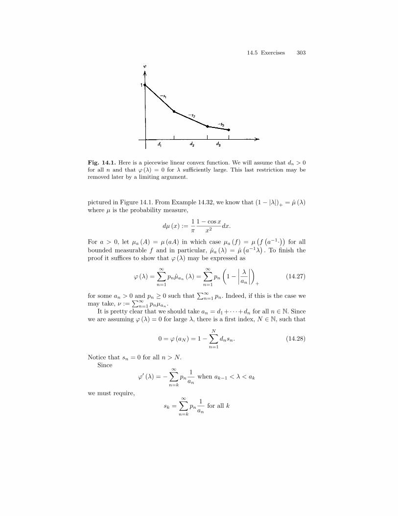
14.5 Exercises 303
Fig. 14.1. Here is a piecewise linear convex function. We will assume that dn > 0for all n and that ϕ (λ) = 0 for λ sufficiently large. This last restriction may beremoved later by a limiting argument.
pictured in Figure 14.1. From Example 14.32, we know that (1− |λ|)+ = µ (λ)where µ is the probability measure,
dµ (x) :=1π
1− cosxx2
dx.
For a > 0, let µa (A) = µ (aA) in which case µa (f) = µ(f(a−1·
))for all
bounded measurable f and in particular, µa (λ) = µ(a−1λ
). To finish the
proof it suffices to show that ϕ (λ) may be expressed as
ϕ (λ) =∞∑
n=1
pnµan(λ) =
∞∑n=1
pn
(1−
∣∣∣∣ λan
∣∣∣∣)+
(14.27)
for some an > 0 and pn ≥ 0 such that∑∞
n=1 pn. Indeed, if this is the case wemay take, ν :=
∑∞n=1 pnµan
.It is pretty clear that we should take an = d1 + · · ·+dn for all n ∈ N. Since
we are assuming ϕ (λ) = 0 for large λ, there is a first index, N ∈ N, such that
0 = ϕ (aN ) = 1−N∑
n=1
dnsn. (14.28)
Notice that sn = 0 for all n > N.Since
ϕ′ (λ) = −∞∑
n=k
pn1an
when ak−1 < λ < ak
we must require,
sk =∞∑
n=k
pn1an
for all k
304 14 Characteristic Functions (Fourier Transform)
which then implies pk1
ak= sk − sk+1 or equivalently that
pk = ak (sk − sk+1) . (14.29)
Since ϕ is convex, we know that −sk ≤ −sk+1 or sk ≥ sk+1 for all k andtherefore pk ≥ 0 and pk = 0 for all k > N. Moreover,
∞∑k=1
pk =∞∑
k=1
ak (sk − sk+1) =∞∑
k=1
aksk −∞∑
k=2
ak−1sk
= a1s1 +∞∑
k=2
sk (ak − ak−1) = d1s1 +∞∑
k=2
skdk
=∞∑
k=1
skdk = 1
where the last equality follows from Eq. (14.28). Working backwards with pk
defined as in Eq. (14.29) it is now easily shown that ddλ
∑∞n=1 pn
(1−
∣∣∣ λan
∣∣∣)+
=
ϕ′ (λ) for λ /∈ a1, a2, . . . and since both functions are equal to 1 at λ = 0we may conclude that Eq. (14.27) is indeed valid.
14.6 Appendix: Bochner’s Theorem
Definition 14.35. A function f ∈ C(Rn,C) is said to have rapid decay orrapid decrease if
supx∈Rn
(1 + |x|)N |f(x)| <∞ for N = 1, 2, . . . .
Equivalently, for each N ∈ N there exists constants CN < ∞ such that|f(x)| ≤ CN (1 + |x|)−N for all x ∈ Rn. A function f ∈ C(Rn,C) is saidto have (at most) polynomial growth if there exists N <∞ such
sup (1 + |x|)−N |f(x)| <∞,
i.e. there exists N ∈ N and C < ∞ such that |f(x)| ≤ C(1 + |x|)N for allx ∈ Rn.
Definition 14.36 (Schwartz Test Functions). Let S denote the space offunctions f ∈ C∞(Rn) such that f and all of its partial derivatives have rapiddecay and let
‖f‖N,α = supx∈Rn
∣∣(1 + |x|)N∂αf(x)∣∣
so thatS =
f ∈ C∞(Rn) : ‖f‖N,α <∞ for all N and α
.
14.6 Appendix: Bochner’s Theorem 305
Also let P denote those functions g ∈ C∞(Rn) such that g and all of itsderivatives have at most polynomial growth, i.e. g ∈ C∞(Rn) is in P iff forall multi-indices α, there exists Nα <∞ such
sup (1 + |x|)−Nα |∂αg(x)| <∞.
(Notice that any polynomial function on Rn is in P.)
Definition 14.37. A function χ : Rn → C is said to be positive (semi)definite iff the matrices A := χ(ξk − ξj)m
k,j=1 are positive definite for allm ∈ N and ξjm
j=1 ⊂ Rn.
Proposition 14.38. Suppose that χ : Rn → C is said to be positive definitewith χ (0) = 1. If χ is continuous at 0 then in fact χ is uniformly continuouson all of Rn.
Proof. Taking ξ1 = x, ξ2 = y and ξ3 = 0 in Definition 14.37 we concludethat
A :=
1 χ (x− y) χ (x)χ (y − x) 1 χ (y)χ (−x) χ (−y) 1
=
1 χ (x− y) χ (x)χ (x− y) 1 χ (y)χ (x) χ (y) 1
is positive definite. In particular,
0 ≤ detA = 1 + χ (x− y)χ (y) χ (x) + χ (x) χ (x− y) χ (y)
− |χ (x)|2 − |χ (y)|2 − |χ (x− y)|2 .
Combining this inequality with the identity,
|χ (x)− χ (y)|2 = |χ (x)|2 + |χ (y)|2 − χ (x) χ (y)− χ (y) χ (x) ,
gives
0 ≤ 1− |χ (x− y)|2 + χ (x− y)χ (y) χ (x) + χ (x) χ (x− y) χ (y)
−|χ (x)− χ (y)|2 + χ (x) χ (y) + χ (y) χ (x)
= 1− |χ (x− y)|2 − |χ (x)− χ (y)|2
+ χ (x− y)χ (y) χ (x)− χ (y) χ (x) + χ (x) χ (x− y) χ (y)− χ (x) χ (y)
= 1− |χ (x− y)|2 − |χ (x)− χ (y)|2 + 2 Re ((χ (x− y)− 1)χ (y) χ (x))
≤ 1− |χ (x− y)|2 − |χ (x)− χ (y)|2 + 2 |χ (x− y)− 1| .
Hence we have
|χ (x)− χ (y)|2 ≤ 1− |χ (x− y)|2 + 2 |χ (x− y)− 1|= (1− |χ (x− y)|) (1 + |χ (x− y)|) + 2 |χ (x− y)− 1|≤ 4 |1− χ (x− y)|
which completes the proof.

306 14 Characteristic Functions (Fourier Transform)
Lemma 14.39. If χ ∈ C(Rn,C) is a positive definite function, then
1. χ(0) ≥ 0.2. χ(−ξ) = χ(ξ) for all ξ ∈ Rn.3. |χ(ξ)| ≤ χ(0) for all ξ ∈ Rn.4. For all f ∈ S(Rd), ∫
Rn×Rn
χ(ξ − η)f(ξ)f(η)dξdη ≥ 0. (14.30)
Proof. Taking m = 1 and ξ1 = 0 we learn χ(0) |λ|2 ≥ 0 for all λ ∈ Cwhich proves item 1. Taking m = 2, ξ1 = ξ and ξ2 = η, the matrix
A :=[
χ(0) χ(ξ − η)χ(η − ξ) χ(0)
]is positive definite from which we conclude χ(ξ−η) = χ(η − ξ) (since A = A∗
by definition) and
0 ≤ det[
χ(0) χ(ξ − η)χ(η − ξ) χ(0)
]= |χ(0)|2 − |χ(ξ − η)|2 .
and hence |χ(ξ)| ≤ χ(0) for all ξ. This proves items 2. and 3. Item 4. followsby approximating the integral in Eq. (14.30) by Riemann sums,∫
Rn×Rn
χ(ξ − η)f(ξ)f(η)dξdη
= limε↓0
ε−2n∑
ξ,η∈(εZn)∩[−ε−1,ε−1]n
χ(ξ − η)f(ξ)f(η) ≥ 0.
The details are left to the reader.
Lemma 14.40. If µ is a finite positive measure on BRn , then χ := µ ∈C(Rn,C) is a positive definite function.
Proof. As has already been observed after Definition ??, the dominatedconvergence theorem implies µ ∈ C(Rn,C). Since µ is a positive measure (andhence real),
µ(−ξ) =∫
Rn
eiξ·xdµ(x) =∫
Rn
e−iξ·xdµ(x) = µ(−ξ).
From this it follows that for any m ∈ N and ξjmj=1 ⊂ Rn, the matrix
A := µ(ξk − ξj)mk,j=1 is self-adjoint. Moreover if λ ∈ Cm,

14.6 Appendix: Bochner’s Theorem 307
m∑k,j=1
µ(ξk − ξj)λkλj =∫
Rn
m∑k,j=1
e−i(ξk−ξj)·xλkλjdµ(x)
=∫
Rn
m∑k,j=1
e−iξk·xλke−iξj ·xλjdµ(x)
=∫
Rn
∣∣∣∣∣m∑
k=1
e−iξk·xλk
∣∣∣∣∣2
dµ(x) ≥ 0
showing A is positive definite.
Theorem 14.41 (Bochner’s Theorem). Suppose χ ∈ C(Rn,C) is positivedefinite function, then there exists a unique positive measure µ on BRn suchthat χ = µ.
Proof. If χ(ξ) = µ(ξ), then for f ∈ S we would have∫Rn
fdµ =∫
Rn
(f∨)ˆ dµ =∫
Rn
f∨(ξ)µ(ξ)dξ.
This suggests that we define
I(f) :=∫
Rn
χ(ξ)f∨(ξ)dξ for all f ∈ S.
We will now show I is positive in the sense if f ∈ S and f ≥ 0 then I(f) ≥ 0.For general f ∈ S we have
I(|f |2) =∫
Rn
χ(ξ)(|f |2
)∨(ξ)dξ =
∫Rn
χ(ξ)(f∨Ff∨
)(ξ)dξ
=∫
Rn
χ(ξ)f∨(ξ − η)f∨(η)dηdξ =∫
Rn
χ(ξ)f∨(ξ − η)f∨(−η)dηdξ
=∫
Rn
χ(ξ − η)f∨(ξ)f∨(η)dηdξ ≥ 0. (14.31)
For t > 0 let pt(x) := t−n/2e−|x|2/2t ∈ S and define
It (x) := IFpt(x) := I(pt(x− ·)) = I(∣∣∣√pt(x− ·)
∣∣∣2)which is non-negative by Eq. (14.31) and the fact that
√pt(x− ·) ∈ S. Using
[pt(x− ·)]∨ (ξ) =∫
Rn
pt(x− y)eiy·ξdy =∫
Rn
pt(y)ei(y+x)·ξdy
= eix·ξp∨t (ξ) = eix·ξe−t|ξ|2/2,

308 14 Characteristic Functions (Fourier Transform)
〈It, ψ〉 =∫
Rn
I(pt(x− ·))ψ(x)dx
=∫
Rn
(∫Rn
χ(ξ) [pt(x− ·)]∨ (ξ)ψ(x)dξ)
dx
=∫
Rn
(∫Rn
χ(ξ)eix·ξe−t|ξ|2/2ψ(x)dξ)
dx
=∫
Rn
χ(ξ)ψ∨(ξ)e−t|ξ|2/2dξ
which coupled with the dominated convergence theorem shows
〈IFpt, ψ〉 →∫
Rn
χ(ξ)ψ∨(ξ)dξ = I(ψ) as t ↓ 0.
Hence if ψ ≥ 0, then I(ψ) = limt↓0〈It, ψ〉 ≥ 0.Let K ⊂ R be a compact set and ψ ∈ Cc(R, [0,∞)) be a function such
that ψ = 1 on K. If f ∈ C∞c (R,R) is a smooth function with supp(f) ⊂ K,then 0 ≤ ‖f‖∞ ψ − f ∈ S and hence
0 ≤ 〈I, ‖f‖∞ ψ − f〉 = ‖f‖∞ 〈I, ψ〉 − 〈I, f〉
and therefore 〈I, f〉 ≤ ‖f‖∞ 〈I, ψ〉. Replacing f by −f implies, −〈I, f〉 ≤‖f‖∞ 〈I, ψ〉 and hence we have proved
|〈I, f〉| ≤ C(supp(f)) ‖f‖∞ (14.32)
for all f ∈ DRn := C∞c (Rn,R) where C(K) is a finite constant for eachcompact subset of Rn. Because of the estimate in Eq. (14.32), it follows thatI|DRn has a unique extension I to Cc(Rn,R) still satisfying the estimates inEq. (14.32) and moreover this extension is still positive. So by the Riesz –Markov Theorem ??, there exists a unique Radon – measure µ on Rn suchthat such that 〈I, f〉 = µ(f) for all f ∈ Cc(Rn,R).
To finish the proof we must show µ(η) = χ(η) for all η ∈ Rn given
µ(f) =∫
Rn
χ(ξ)f∨(ξ)dξ for all f ∈ C∞c (Rn,R). (14.33)
Let f ∈ C∞c (Rn,R+) be a radial function such f(0) = 1 and f(x) is decreasingas |x| increases. Let fε(x) := f(εx), then by Theorem ??,
F−1[e−iηxfε(x)
](ξ) = ε−nf∨(
ξ − η
ε)
and therefore, from Eq. (14.33),∫Rn
e−iηxfε(x)dµ(x) =∫
Rn
χ(ξ)ε−nf∨(ξ − η
ε)dξ. (14.34)

14.7 Appendix: A Multi-dimensional Weirstrass Approximation Theorem 309
Because∫
Rn f∨(ξ)dξ = Ff∨(0) = f(0) = 1, we may apply the approximate δ
– function Theorem ?? to Eq. (14.34) to find∫Rn
e−iηxfε(x)dµ(x) → χ(η) as ε ↓ 0. (14.35)
On the the other hand, when η = 0, the monotone convergence theoremimplies µ(fε) ↑ µ(1) = µ(Rn) and therefore µ(Rn) = µ(1) = χ(0) < ∞. Nowknowing the µ is a finite measure we may use the dominated convergencetheorem to concluded
µ(e−iηxfε(x)) → µ(e−iηx) = µ(η) as ε ↓ 0
for all η. Combining this equation with Eq. (14.35) shows µ(η) = χ(η) for allη ∈ Rn.
14.7 Appendix: A Multi-dimensional WeirstrassApproximation Theorem
The following theorem is the multi-dimensional generalization of Theorem4.23.
Theorem 14.42 (Weierstrass Approximation Theorem). Suppose thatK = [a1, b1] × . . . [ad, bd] with −∞ < ai < bi < ∞ is a compact rectangle inRd. Then for every f ∈ C(K,C), there exists polynomials pn on Rd such thatpn → f uniformly on K.
Proof. By a simple scaling and translation of the arguments of f we mayassume with out loss of generality that K = [0, 1]d . By considering the realand imaginary parts of f separately, it suffices to assume f ∈ C([0,1],R).
Given x ∈ K, letXn =
(X1
n, . . . , Xdn
)∞n=1
be i.i.d. random vectors withvalues in Rd such that
P (Xn = ε) =d∏
i=1
(1− xi)1−εi xεi
i
for all ε = (ε1, . . . , εd) ∈ 0, 1d. Since each Xj
n is a Bernoulli random variablewith P
(Xj
n = 1)
= xj , we know that
EXn = x and Var(Xj
n
)= xj − x2
j = xj(1− xj).
As usual let Sn = Sn := X1 + · · ·+Xn ∈ Rd, then

310 14 Characteristic Functions (Fourier Transform)
E[Sn
n
]= x and
E
[∥∥∥∥Sn
n− x
∥∥∥∥2]
=d∑
j=1
E(Sj
n
n− xj
)2
=d∑
j=1
Var(Sj
n
n− xj
)
=d∑
j=1
Var(Sj
n
n
)=
1n2
·d∑
j=1
n∑k=1
Var(Xj
k
)
=1n
d∑j=1
xj(1− xj) ≤d
4n.
This shows Sn/n→ x in L2 (P ) and hence by Chebyshev’s inequality, Sn/nP→
x in and by a continuity theorem, f(
Sn
n
) P→ f (x) as n→∞. This along withthe dominated convergence theorem shows
pn(x) := E[f
(Sn
n
)]→ f (x) as n→∞, (14.36)
where
pn(x) =∑
ε(·)∈0,1d
f
(ε (1) + · · ·+ ε (n)
n
)P (X1 = ε (1) , . . . , Xn = ε (n))
=∑
ε(·)∈0,1d
f
(ε (1) + · · ·+ ε (n)
n
) n∏k=1
d∏i=1
(1− xi)1−εi(k)
xεi(k)i
is a polynomial of degree nd. In fact more is true.Suppose ε > 0 is given, M = sup |f(x)| : x ∈ K , and
δε = sup |f(y)− f(x)| : x, y ∈ K and ‖y − x‖ ≤ ε .
By uniform continuity of f on K, limε↓0 δε = 0. Therefore,
|f(x)− pn(x)| =∣∣∣∣E(f(x)− f(
Sn
n))∣∣∣∣ ≤ E
∣∣∣∣f(x)− f(Sn
n)∣∣∣∣
≤E[∣∣∣∣f(x)− f(
Sn
n)∣∣∣∣ : ‖Sn − x‖ > ε
]+ E
[∣∣∣∣f(x)− f(Sn
n)∣∣∣∣ : ‖Sn − x‖ ≤ ε
]≤2MP (‖Sn − x‖ > ε) + δε. (14.37)
By Chebyshev’s inequality,
P (‖Sn − x‖ > ε) ≤ 1ε2
E ‖Sn − x‖2 =d
4nε2,

14.7 Appendix: A Multi-dimensional Weirstrass Approximation Theorem 311
and therefore, Eq. (14.37) yields the estimate
supx∈K
|f (x)− pn (x)| ≤ 2dMnε2
+ δε
and hencelim sup
n→∞supx∈K
|f (x)− pn (x)| ≤ δε → 0 as ε ↓ 0.
Here is a version of the complex Weirstrass approximation theorem.
Theorem 14.43 (Complex Weierstrass Approximation Theorem).Suppose that K ⊂ Cd ∼= Rd × Rd is a compact rectangle. Then there ex-ists polynomials in (z = x+ iy, z = x− iy) , pn(z, z) for z ∈ Cd, such thatsupz∈K |qn(z, z)− f(z)| → 0 as n→∞ for every f ∈ C (K,C) .
Proof. The mapping (x, y) ∈ Rd×Rd → z = x+iy ∈ Cd is an isomorphismof vector spaces. Letting z = x− iy as usual, we have x = z+z
2 and y = z−z2i .
Therefore under this identification any polynomial p(x, y) on Rd×Rd may bewritten as a polynomial q in (z, z), namely
q(z, z) = p(z + z
2,z − z
2i).
Conversely a polynomial q in (z, z) may be thought of as a polynomial p in(x, y), namely p(x, y) = q(x + iy, x − iy). Hence the result now follows fromTheorem 14.42.
Example 14.44. Let K = S1 = z ∈ C : |z| = 1 and A be the set of polyno-mials in (z, z) restricted to S1. Then A is dense in C(S1). To prove this firstobserve if f ∈ C
(S1)
then F (z) = |z| f( z|z| ) for z 6= 0 and F (0) = 0 defines
F ∈ C(C) such that F |S1 = f. By applying Theorem 14.43 to F restricted toa compact rectangle containing S1 we may find qn (z, z) converging uniformlyto F on K and hence on S1. Since z = z−1 on S1, we have shown polynomialsin z and z−1 are dense in C(S1). This example generalizes in an obvious wayto K =
(S1)d ⊂ Cd.
Exercise 14.6. Use Example 14.44 to show that any 2π – periodic continuousfunction, g : Rd → C, may be uniformly approximated by a trigonometricpolynomial of the form
p (x) =∑λ∈Λ
aλeiλ·x
where Λ is a finite subset of Zd and aλ ∈ C for all λ ∈ Λ. Hint: start byshowing there exists a unique continuous function, f :
(S1)d → C such that
f(eix1 , . . . , eixd
)= F (x) for all x = (x1, . . . , xd) ∈ Rd.

312 14 Characteristic Functions (Fourier Transform)
Solution to Exercise (14.6). I will write out the solution when d = 1. Forz ∈ S1, define F (z) := f(eiθ) where θ ∈ R is chosen so that z = eiθ. Sincef is 2π – periodic, F is well defined since if θ solves eiθ = z then all othersolutions are of the form θ + 2πn : n ∈ Z . Since the map θ → eiθ is a local
homeomorphism, i.e. for any J = (a, b) with b−a < 2π, the map θ ∈ J φ→ J :=eiθ : θ ∈ J
⊂ S1 is a homeomorphism, it follows that F (z) = f φ−1(z) for
z ∈ J . This shows F is continuous when restricted to J . Since such sets coverS1, it follows that F is continuous. It now follows from Example 14.44 thatpolynomials in z and z−1 are dense in C(S1). Hence for any ε > 0 there exists
p(z, z) =∑
am,nzmzn =
∑am,nz
mz−n =∑
am,nzm−n
such that |F (z)− p(z, z)| ≤ ε for all z. Taking z = eiθ then implies thereexists bn ∈ C and N ∈ N such that
pε (θ) :=N∑
n=−N
bneinθ (14.38)
satisfiessup
θ
∣∣f(θ)− p (θ)∣∣ ≤ ε.
Exercise 14.7. Suppose f ∈ C (R,C) is a 2π – periodic function (i.e.f (x+ 2π) = f (x) for all x ∈ R) and∫ 2π
0
f (x) einxdx = 0 for all n ∈ Z,
show again that f ≡ 0. Hint: Use Exercise 14.6.
Solution to Exercise (14.7). By assumption,∫ 2π
0f (θ) einθdθ = 0 for all n
and so by the linearity of the Riemann integral,
0 =∫ 2π
0
f (θ) pε (θ) dθ. (14.39)
Choose trigonometric polynomials, pε, as in Eq. (14.38) such that pε (θ) →f (θ) uniformly in θ as ε ↓ 0. Passing to the limit in Eq. (14.39) implies
0 = limε↓0
∫ 2π
0
f (θ) pε (θ) dθ =∫ 2π
0
f (θ) f (θ) dθ =∫ 2π
0
|f (θ)|2 dθ.
From this it follows that f ≡ 0, for if |f (θ0)| > 0 for some θ0 then |f (θ)| ≥ε > 0 for θ in a neighborhood of θ0 by continuity of f. It would then followthat
∫ 2π
0|f (θ)|2 dθ > 0.

14.8 Appendix: Some Calculus Estimates 313
14.8 Appendix: Some Calculus Estimates
We end this section by gathering together a number of calculus estimates thatwe will need in the future.
1. Taylor’s theorem with integral remainder states, if f ∈ Ck (R) andz,∆ ∈ R or f be holomorphic in a neighborhood of z ∈ C and ∆ ∈ C besufficiently small so that f (z + t∆) is defined for t ∈ [0, 1] , then
f (z +∆) =k−1∑n=0
f (n) (z)∆n
n!+∆krk (z,∆) (14.40)
=k−1∑n=0
f (n) (z)∆n
n!+∆k
[1k!f (k) (z) + ε (z,∆)
](14.41)
where
rk (z,∆) =1
(k − 1)!
∫ 1
0
f (k) (z + t∆) (1− t)k−1dt (14.42)
=1k!f (k) (z) + ε (z,∆) (14.43)
and
ε (z,∆) =1
(k − 1)!
∫ 1
0
[f (k) (z + t∆)− f (k) (z)
](1− t)k−1
dt→ 0 as ∆→ 0.
(14.44)To prove this, use integration by parts to show,
rk (z,∆) =1k!
∫ 1
0
f (k) (z + t∆)(− d
dt
)(1− t)k
dt
= − 1k!
[f (k) (z + t∆) (1− t)k
]t=1
t=0+∆
k!
∫ 1
0
f (k+1) (z + t∆) (1− t)kdt
=1k!f (k) (z) +∆rk+1 (z,∆) ,
i.e.∆krk (z,∆) =
1k!f (k) (z)∆k +∆k+1rk+1 (z,∆) .
The result now follows by induction.2. For y ∈ R, sin y = y
∫ 1
0cos (ty) dt and hence
|sin y| ≤ |y| . (14.45)
3. For y ∈ R we have
cos y = 1 + y2
∫ 1
0
− cos (ty) (1− t) dt ≥ 1 + y2
∫ 1
0
− (1− t) dt = 1− y2
2.

314 14 Characteristic Functions (Fourier Transform)
Equivalently put2,
g (y) := cos y − 1 + y2/2 ≥ 0 for all y ∈ R. (14.46)
4. Since
|ez − 1− z| =∣∣∣∣z2
∫ 1
0
etz (1− t) dt∣∣∣∣ ≤ |z|2
∫ 1
0
et Re z (1− t) dt,
if Re z ≤ 0, then|ez − 1− z| ≤ |z|2 /2 (14.47)
and if Re z > 0 then
|ez − 1− z| ≤ eRe z |z|2 /2.
Combining these into one estimate gives,
|ez − 1− z| ≤ e0∨Re z · |z|2
2. (14.48)
5. Since eiy − 1 = iy∫ 1
0eitydt,
∣∣eiy − 1∣∣ ≤ |y| and hence∣∣eiy − 1
∣∣ ≤ 2 ∧ |y| for all y ∈ R. (14.49)
Lemma 14.45. For z = reiθ with −π < θ < π and r > 0, let ln z = ln r+ iθ.Then ln : C \ (−∞, 0] → C is a holomorphic function such that eln z = z3 andif |z| < 1 then2 Alternatively,
|sin y| =Z y
0
cos xdx
≤Z y
0
|cos x| dx
≤ |y|
and for y ≥ 0 we have,
cos y − 1 =
Z y
0
− sin xdx ≥Z y
0
−xdx = −y2/2.
This last inequality may also be proved as a simple calculus exercise followingfrom; g (±∞) = ∞ and g′ (y) = 0 iff sin y = y which happens iff y = 0.
3 For the purposes of this lemma it suffices to define ln (1 + z) = −P∞
n=1 (−z)n /nand to then observe: 1)
d
dzln (1 + z) =
∞Xn=0
(−z)n =1
1 + z,
and 2) the functions 1 + z and eln(1+z) both solve
f ′ (z) =1
1 + zf (z) with f (0) = 1
and therefore eln(1+z) = 1 + z.
14.8 Appendix: Some Calculus Estimates 315
|ln (1 + z)− z| ≤ |z|2 12 (1− |z|)2
for |z| < 1. (14.50)
Proof. Clearly eln z = z and ln z is continuous. Therefore by the inversefunction theorem for holomorphic functions, ln z is holomorphic and
zd
dzln z = eln z d
dzln z = 1.
Therefore, ddz ln z = 1
z and d2
dz2 ln z = − 1z2 . So by Taylor’s theorem,
ln (1 + z) = z − z2
∫ 1
0
1(1 + tz)2
(1− t) dt. (14.51)
If t ≥ 0 and |z| < 1, then∣∣∣∣ 1(1 + tz)
∣∣∣∣ ≤ ∞∑n=0
|tz|n =1
1− t |z|≤ 1
1− |z|.
and therefore, ∣∣∣∣∣∫ 1
0
1(1 + tz)2
(1− t) dt
∣∣∣∣∣ ≤ 12 (1− |z|)2
. (14.52)
Eq. (14.50) is now a consequence of Eq. (14.51) and Eq. (14.52).
Lemma 14.46. For all y ∈ R and n ∈ N∪0 ,∣∣∣∣∣eiy −n∑
k=0
(iy)k
k!
∣∣∣∣∣ ≤ |y|n+1
(n+ 1)!(14.53)
and in particular, ∣∣∣∣eiy −(
1 + iy − y2
2!
)∣∣∣∣ ≤ y2 ∧ |y|3
3!. (14.54)
More generally for all n ∈ N we have∣∣∣∣∣eiy −n∑
k=0
(iy)k
k!
∣∣∣∣∣ ≤ |y|n+1
(n+ 1)!∧ 2 |y|n
n!. (14.55)
Proof. By Taylor’s theorem (see Eq. (14.40) with f (y) = eiy, x = 0 and∆ = y) we have∣∣∣∣∣eiy −
n∑k=0
(iy)k
k!
∣∣∣∣∣ =∣∣∣∣yn+1
n!
∫ 1
0
in+1eity (1− t)ndt
∣∣∣∣≤ |y|n+1
n!
∫ 1
0
(1− t)ndt =
|y|n+1
(n+ 1)!

316 14 Characteristic Functions (Fourier Transform)
which is Eq. (14.53). Using Eq. (14.53) with n = 1 implies∣∣∣∣eiy −(
1 + iy − y2
2!
)∣∣∣∣ ≤ ∣∣eiy − (1 + iy)∣∣+ ∣∣∣∣y2
2
∣∣∣∣≤∣∣∣∣y2
2
∣∣∣∣+ ∣∣∣∣y2
2
∣∣∣∣ = y2
and using Eq. (14.53) with n = 2 implies∣∣∣∣eiy −(
1 + iy − y2
2!
)∣∣∣∣ ≤ |y|3
3!.
Combining the last two inequalities completes the proof of Eq. (14.54). Equa-tion (14.55) is proved similarly and hence will be omitted.

15
Weak Convergence of Random Sums
Throughout this chapter, we will assume the following standing notation un-less otherwise stated. For each n ∈ N, let Xn,kn
k=1 be independent randomvariables and let
Sn :=n∑
k=1
Xn,k. (15.1)
Until further notice we are going to assume E [Xn,k] = 0, σ2n,k = E
[X2
n,k
]<
∞, and Var (Sn) =∑n
k=1 σ2n,k = 1. Also let
fnk (λ) := E[eiλXn,k
](15.2)
denote the characteristic function of Xn,k.
Example 15.1. Suppose Xn∞n=1 are mean zero square integrable randomvariables with σ2
k = Var (Xn) . If we let s2n :=∑n
k=1 Var (Xk) =∑n
k=1 σ2k,
σ2n,k := σ2
k/s2n, and Xn,k := Xk/sn, then Xn,kn
k=1 satisfy the above hypoth-esis and Sn = 1
sn
∑nk=1Xk.
Our main interest in this chapter is to consider the limiting behavior ofSn as n → ∞. In order to do this, it will be useful to put conditions on theXn,k such that no one term dominates sum defining the sum defining Sn inEq. (15.1) in the limit as n→∞.
Definition 15.2. We say that Xn,k satisfies the Lindeberg Condition(LC) if for all t > 0,
limn→∞
n∑k=1
E[X2
n,k1|Xn,k|>t
]= 0. (15.3)
We say Xn,k satisfies condition (M) if
Dn := maxσ2
n,k : k ≤ n→ 0 as n→∞, (15.4)
and we say Xn,k is uniformly asymptotic negligibility (UAN) if forall ε > 0,
limn→∞
maxk≤n
P (|Xn,k| > ε) = 0. (15.5)

318 15 Weak Convergence of Random Sums
Remark 15.3. The reader should observe that in order for condition (M) tohold in the setup in Example 15.1 it is necessary that limn→∞ s2n = ∞.
Lemma 15.4. Let Xn,k∞n=1 be as above, then (LC) =⇒ (M) =⇒(UAN) .
Proof. For k ≤ n,
σ2n,k = E
[X2
n,k
]= E
[X2
n,k1|Xn,k|≤t
]+ E
[X2
n,k1|Xn,k|>t
]≤ t2 + E
[X2
n,k1|Xn,k|>t
]≤ t2 +
n∑m=1
E[X2
n,m1|Xn,m|>t
]and therefore using (LC) we find
limn→∞
maxk≤n
σ2n,k ≤ t2 for all t > 0.
This clearly implies (M) holds. The assertion that (M) implies (UAN) followsby Chebyschev’s inequality,
maxk≤n
P (|Xn,k| > ε) ≤ maxk≤n
1ε2
E[|Xn,k|2 : |Xn,k| > ε
]≤ 1ε2
n∑k=1
E[|Xn,k|2 : |Xn,k| > ε
]→ 0.
In fact the same argument shows that (M) implies
n∑k=1
P (|Xn,k| > ε) ≤ 1ε2
n∑k=1
E[|Xn,k|2 : |Xn,k| > ε
]→ 0.
We will need the following lemma for our subsequent applications of thecontinuity theorem.
Lemma 15.5. Suppose that ai, bi ∈ C with |ai| , |bi| ≤ 1 for i = 1, 2, . . . , n.Then ∣∣∣∣∣
n∏i=1
ai −n∏
i=1
bi
∣∣∣∣∣ ≤n∑
i=1
|ai − bi| .
Proof. Let a :=∏n−1
i=1 ai and b :=∏n−1
i=1 bi and observe that |a| , |b| ≤ 1and that
|ana− bnb| ≤ |ana− anb|+ |anb− bnb|= |an| |a− b|+ |an − bn| |b|≤ |a− b|+ |an − bn| .
The proof is now easily completed by induction on n.

15 Weak Convergence of Random Sums 319
Lemma 15.6. If X is a square integrable random variable, then
f (λ) := E[eiλX
]= 1 + iλEX − λ2
2!E[X2]+ r (λ)
where
r (λ) := λ2E
[X2 ∧ |λ| |X|
3
3!
]= λ2ε (λ)
and
ε (λ) := E
[X2 ∧ |λ| |X|
3
3!
]→ 0 as λ→ 0. (15.6)
Proof. Using Eq. (14.54) with y = λX and taking expectations implies,∣∣∣∣f (λ)−(
1 + iλEX − λ2
2!E[X2])∣∣∣∣ ≤ E
∣∣∣∣eiλX −(
1 + iλX − λ2X2
2!
)∣∣∣∣≤ λ2E
[X2 ∧ |λ| |X|
3
3!
]=: λ2ε (λ) .
The DCT, with X2 ∈ L1 (P ) being the dominating function, allows us toconclude that limε→0 ε (λ) = 0.
Theorem 15.7 (Lindeberg-Feller CLT (I)). Suppose Xn∞n=1 is a se-quence of random variables satisfying (LC) , then
Sn =⇒ N (0, 1) . (15.7)
(See Theorem 15.11 for a converse to this theorem.)
Proof. Our goal is to show, E[eiλSn
]→ e−λ2/2 as n→∞. Since
E[eiλSn
]=
n∏k=1
fnk (λ) and e−λ2/2 =n∏
k=1
e−λ2σ2n,k/2,
we may use Lemma 15.5 to conclude,∣∣∣E [eiλSn]− e−λ2/2
∣∣∣ ≤ n∑k=1
∣∣∣fnk (λ)− e−λ2σ2n,k/2
∣∣∣ = n∑k=1
(An,k +Bn,k)
where
An,k :=
∣∣∣∣∣fnk (λ)−
[1−
λ2σ2n,k
2
]∣∣∣∣∣ and
Bn,k :=
∣∣∣∣∣[1−
λ2σ2n,k
2
]− e−λ2σ2
n,k/2
∣∣∣∣∣ .

320 15 Weak Convergence of Random Sums
Now, using Lemma 15.6,
An,k =∣∣∣∣E [eiλXn,k − 1 +
λ2
2X2
n,k
]∣∣∣∣ ≤ E∣∣∣∣eiλXn,k − 1 +
λ2
2X2
n,k
∣∣∣∣≤ λ2E
[Xn,k ∧
|λ| |Xn,k|3
3!
]
≤ λ2E
[Xn,k ∧
|λ| |Xn,k|3
3!: |Xn,k| ≤ ε
]+ λ2E
[X2
n,k ∧|λ| |Xn,k|3
3!: |Xn,k| > ε
]
≤ λ2E
[|λ| |Xn,k|3
3!: |Xn,k| ≤ ε
]+ λ2E
[X2
n,k : |Xn,k| > ε]
≤ λ2
3!|λ| ε · E
[|Xn,k|2 : |Xn,k| ≤ ε
]+ λ2E
[X2
n,k : |Xn,k| > ε]
=|λ|3 ε
6σ2
n,k + λ2E[X2
n,k : |Xn,k| > ε].
From this estimate and (LC) it follows that
lim supn→∞
n∑k=1
An,k ≤ lim supn→∞
(λ3ε
6+ λ2
n∑k=1
E[X2
n,k : |Xn,k| > ε])
=λ3ε
6
and since ε > 0 is arbitrary, we may conclude that lim supn→∞∑n
k=1An,k = 0.To estimate
∑nk=1Bn,k, we use the estimate, |e−u − 1 + u| ≤ u2/2 valid
for u ≥ 0 (see Eq. 14.47 with z = −u). With this estimate we find,
n∑k=1
Bn,k =n∑
k=1
∣∣∣∣∣[1−
λ2σ2n,k
2
]− e−λ2σ2
n,k/2
∣∣∣∣∣≤
n∑k=1
12
[λ2σ2
n,k
2
]2
=λ4
8
n∑k=1
σ4n,k
≤ λ4
8maxk≤n
σ2n,k
n∑k=1
σ2n,k =
λ4
8maxk≤n
σ2n,k → 0,
wherein we have used (M) (which is implied by (LC)) in taking the limit asn→∞.
As an application of Theorem 15.7 we can give half of the proof of Theorem12.12.
Theorem 15.8 (Converse assertion in Theorem 12.12). If Xn∞n=1 areindependent random variables and the random series,
∑∞n=1Xn, is almost
surely convergent, then for all c > 0 the following three series converge;
Proof.

15 Weak Convergence of Random Sums 321
1.∑∞
n=1 P (|Xn| > c) <∞,2.∑∞
n=1 Var(Xn1|Xn|≤c
)<∞, and
3.∑∞
n=1 E(Xn1|Xn|≤c
)converges.
Proof. Since∑∞
n=1Xn is almost surely convergent, it follows thatlimn→∞Xn = 0 a.s. and hence for every c > 0, P (|Xn| ≥ c i.o.) =0. According the Borel zero one law this implies for every c > 0that
∑∞n=1 P (|Xn| > c) < ∞. Given this, we now know that Xn and
Xcn := Xn1|Xn|≤c
are tail equivalent for all c > 0 and in particular
∑∞n=1X
cn
is almost surely convergent for all c > 0.Fix c > 0 and let Yn := Xc
n − E [Xcn] = Xc
n − µn Let
s2n = Var (Y1 + · · ·+ Yn) =n∑
k=1
σ2k.
For the sake of contradictions, suppose s2n → ∞ as n → ∞. Since |Yk| ≤ 2c,it follows that
∑nk=1 E
[Y 2
k 1|Yk|>snt
]= 0 for all sufficiently large n and hence
limn→∞
1s2n
n∑k=1
E[Y 2
k 1|Yk|>snt
]= 0,
i.e. Yn,k : Yk/sn∞n=1 satisfies (LC) , cf. Examples 15.1 and Remark 15.3. Soby the central limit theorem, it follows that
Xc1 − µ1 + · · ·+Xc
n − µn
s2n=Y1 + · · ·+ Yn
s2n=⇒ N (0, 1) .
On the other hand we know
Xc1 + · · ·+Xc
n
s2n→ 0 a.s.
and thereforeY1 + · · ·+ Yn
s2n→ c := − lim
n→∞
1s2n
n∑k=1
µk
which is constant and hence not a standard normal random variable. Thus wemust conclude that
∞∑n=1
Var(Xn1|Xn|≤c
)=∞∑
n=1
Var (Xcn) =
∞∑k=1
σ2k = lim
n→∞s2n <∞.
An application of Kolmogorov’s convergence criteria (Theorem 12.11) im-plies that
∞∑n=1
(Xcn − µn) is convergent a.s.

322 15 Weak Convergence of Random Sums
Since we already know that∑∞
n=1Xcn is convergent almost surely we may now
conclude∞∑
n=1
E(Xn1|Xn|≤c
)=∞∑
n=1
µn is convergent.
Let us now turn to the converse of Theorem 15.7, see Theorem 15.11 below.
Lemma 15.9. Let X be a random variable such that EX2 <∞ and EX = 0.Further let f (λ) := E
[eiλX
]and u (λ) := Re (f (λ)− 1) . Then for all c > 0,
u (λ) +λ2
2E[X2]≥ E
[X2
[λ2
2− 2c2
]: |X| > c
](15.8)
or equivalently
E[cosλX − 1 +
λ2
2X2
]≥ E
[X2
[λ2
2− 2c2
]: |X| > c
]. (15.9)
In particular if we choose |λ| ≥√
6/ |c| , then
E[cosλX − 1 +
λ2
2X2
]≥ 1c2
E[X2 : |X| > c
]. (15.10)
Proof. For all λ ∈ R, we have (see Eq. (14.46)) cosλX − 1 + λ2
2 X2 ≥ 0
and cosλX − 1 ≥ −2. Therefore,
u (λ) +λ2
2E[X2]
= E[cosλX − 1 +
λ2
2X2
]≥ E
[cosλX − 1 +
λ2
2X2 : |X| > c
]≥ E
[−2 +
λ2
2X2 : |X| > c
]≥ E
[−2
|X|2
c2+λ2
2X2 : |X| > c
]
which gives Eq. (15.8).
Lemma 15.10. Suppose that Xn,k satisfies property (M) , i.e. Dn :=maxk≤n σ
2n,k → 0. If we define,
ϕn,k (λ) := fn,k (λ)− 1 = E[eiλXn,k − 1
],
then;
1. limn→∞maxk≤n |ϕn,k (λ)| = 0 and

15 Weak Convergence of Random Sums 323
2. fSn(λ)−
∏nk=1 e
ϕn,k(λ) → 0 as n→∞, where
fSn (λ) = E[eiλSn
]=
n∏k=1
fn,k (λ) .
Proof. For the first item we estimate,∣∣EeiλX − 1∣∣ ≤ E
∣∣eiλX − 1∣∣ ≤ E [2 ∧ |λX|]
= E [2 ∧ |λX| : |X| ≥ ε] + E [2 ∧ |λX| : |X| < ε]
≤ 2P [|X| ≥ ε] + |λ| ε ≤ 2ε2
E |X|2 + |λ| ε
Replacing X by Xn,k and in the above inequality shows
|ϕn,k (λ)| = |fn,k (λ)− 1| ≤ 2ε2
E |Xn,k|2 + |λ| ε =2σ2
n,k
ε2+ |λ| ε.
Therefore,
lim supn→∞
maxk≤n
|ϕn,k (λ)| ≤ lim supn→∞
[2Dn
ε2+ |λ| ε
]= |λ| ε→ 0 as ε ↓ 0.
For the second item, observe that Reϕn,k (λ) = Re fn,k (λ) − 1 ≤ 0 andhence ∣∣∣eϕn,k(λ)
∣∣∣ = eRe ϕn,k(λ) ≤ e0 = 1
and hence we have from Lemma 15.5 and the estimate (14.47),∣∣∣∣∣n∏
k=1
fn,k (λ)−n∏
k=1
eϕn,k(λ)
∣∣∣∣∣ ≤n∑
k=1
∣∣∣fn,k (λ)− eϕn,k(λ)∣∣∣
=n∑
k=1
∣∣∣eϕn,k(λ) − 1− ϕn,k (λ)∣∣∣
≤ 12
n∑k=1
|ϕn,k (λ)|2
≤ 12
maxk≤n
|ϕn,k (λ)| ·n∑
k=1
|ϕn,k (λ)| .
Moreover since EXn,k = 0, the estimate in Eq. (14.47) implies
n∑k=1
|ϕn,k (λ)| =n∑
k=1
∣∣E [eiλXn,k − 1− iλXn,k
]∣∣≤
n∑k=1
∣∣∣∣E [12|λXn,k|2
]∣∣∣∣ ≤ λ2
2
n∑k=1
σ2n,k =
λ2
2.
324 15 Weak Convergence of Random Sums
Thus we have shown,∣∣∣∣∣n∏
k=1
fn,k (λ)−n∏
k=1
eϕn,k(λ)
∣∣∣∣∣ ≤ λ2
4maxk≤n
|ϕn,k (λ)|
and the latter expression tends to zero by item 1.
Theorem 15.11 (Lindeberg-Feller CLT (II)). Suppose Xn∞n=1 is a se-quence of random variables satisfying (M) and also the central limit theoremin Eq. (15.7), then Xn∞n=1 satisfies (LC) .
Proof. By assumption we have
limn→∞
maxk≤n
σ2n,k = 0 and lim
n→∞
n∏k=1
fn,k (λ) = e−λ2/2.
The second inequality combined with Lemma 15.10 implies,
limn→∞
ePn
k=1 ϕn,k(λ) = limn→∞
n∏k=1
eϕn,k(λ) = e−λ2/2
and taking the modulus of this equation then implies,
limn→∞
ePn
k=1 Re ϕn,k(λ) = limn→∞
∣∣∣ePnk=1 ϕn,k(λ)
∣∣∣ = e−λ2/2
from which we may conclude
limn→∞
n∑k=1
Reϕn,k (λ) = −λ2/2.
We may write this last limit as
limn→∞
n∑k=1
E[cos (λXn,k)− 1 +
λ2
2X2
n,k
]= 0
which by Lemma 15.9 implies
limn→∞
n∑k=1
E[X2
n,k : |Xn,k| > c]
= 0
for all c > 0.
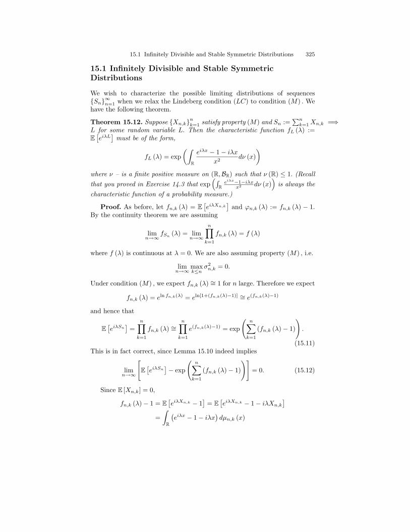
15.1 Infinitely Divisible and Stable Symmetric Distributions 325
15.1 Infinitely Divisible and Stable SymmetricDistributions
We wish to characterize the possible limiting distributions of sequencesSn∞n=1 when we relax the Lindeberg condition (LC) to condition (M) . Wehave the following theorem.
Theorem 15.12. Suppose Xn,knk=1 satisfy property (M) and Sn :=
∑nk=1Xn,k =⇒
L for some random variable L. Then the characteristic function fL (λ) :=E[eiλL
]must be of the form,
fL (λ) = exp(∫
R
eiλx − 1− iλx
x2dν (x)
)where ν – is a finite positive measure on (R,BR) such that ν (R) ≤ 1. (Recallthat you proved in Exercise 14.3 that exp
(∫R
eiλx−1−iλxx2 dν (x)
)is always the
characteristic function of a probability measure.)
Proof. As before, let fn,k (λ) = E[eiλXn,k
]and ϕn,k (λ) := fn,k (λ) − 1.
By the continuity theorem we are assuming
limn→∞
fSn(λ) = lim
n→∞
n∏k=1
fn,k (λ) = f (λ)
where f (λ) is continuous at λ = 0. We are also assuming property (M) , i.e.
limn→∞
maxk≤n
σ2n,k = 0.
Under condition (M) , we expect fn,k (λ) ∼= 1 for n large. Therefore we expect
fn,k (λ) = eln fn,k(λ) = eln[1+(fn,k(λ)−1)] ∼= e(fn,k(λ)−1)
and hence that
E[eiλSn
]=
n∏k=1
fn,k (λ) ∼=n∏
k=1
e(fn,k(λ)−1) = exp
(n∑
k=1
(fn,k (λ)− 1)
).
(15.11)This is in fact correct, since Lemma 15.10 indeed implies
limn→∞
[E[eiλSn
]− exp
(n∑
k=1
(fn,k (λ)− 1)
)]= 0. (15.12)
Since E [Xn,k] = 0,
fn,k (λ)− 1 = E[eiλXn,k − 1
]= E
[eiλXn,k − 1− iλXn,k
]=∫
R
(eiλx − 1− iλx
)dµn,k (x)

326 15 Weak Convergence of Random Sums
where µn,k := P X−1n,k is the law of Xn,k. Therefore we have
exp
(n∑
k=1
(fn,k (λ)− 1)
)= exp
(n∑
k=1
∫R
(eiλx − 1− iλx
)dµn,k (x)
)
= exp
(∫R
(eiλx − 1− iλx
) n∑k=1
dµn,k (x)
)
= exp(∫
R
(eiλx − 1− iλx
)dν∗n (x)
)(15.13)
where ν∗n :=∑n
k=1 µn,k. Let us further observe that∫Rx2dν∗n (x) =
n∑k=1
∫Rx2dµn,k (x) =
n∑k=1
σ2n,k = 1.
Hence if we define dν∗ (x) := x2dν∗n (x) , then νn is a probability measure andwe have from Eqs. (15.12) and Eq. (15.13) that∣∣∣∣fSn (λ)− exp
(∫R
eiλx − 1− iλx
x2dνn (x)
)∣∣∣∣→ 0. (15.14)
Since h (x) := eiλx−1−iλxx2 is a continuous function of R with h (±∞) = 0, there
is a subsequence, nl of n such that νnl(h) → ν (h) for some probability
measure on(R,BR
). Combining this with Eq. (15.14) allows us to conclude,
fL (λ) = liml→∞
E[eiλSnl
]= lim
l→∞exp
(∫R
(eiλx − 1− iλx
)dν∗nl
(x))
= exp(∫
R
eiλx − 1− iλx
x2dν (x)
).
Definition 15.13. We say that Xn,knk=1 has bounded variation (BV ) iff
supn
Var (Sn) = supn
n∑k=1
σ2n,k <∞. (15.15)
Corollary 15.14. Suppose Xn,knk=1 satisfy properties (M) and (BV ) . If
Sn :=∑n
k=1Xn,k =⇒ L for some random variable L, then
fL (λ) = exp(∫
R
eiλx − 1− iλx
x2dν (x)
)(15.16)
where ν – is a finite positive measure on (R,BR) .

15.1 Infinitely Divisible and Stable Symmetric Distributions 327
Proof. Let s2n := Var (Sn) . If limn→∞ sn = 0, then Sn → 0 in L2 andhence weakly, therefore Eq. (15.16) holds with ν ≡ 0. So let us now sup-pose limn→∞ sn 6= 0. Since sn∞n=1 is bounded, we may by passing to asubsequence if necessary, assume limn→∞ sn = s > 0. By replacing Xn,k
by Xn,k/sn and hence Sn by Sn/sn, we then know by Slutsky’s theorem thatSn/sn =⇒ L/s. Hence by an application of Theorem 15.12, we may conclude
fL (λ/s) = fL/s (λ) = exp(∫
R
eiλx − 1− iλx
x2dν (x)
)where ν – is a finite positive measure on (R,BR) such that ν (R) ≤ 1. Lettingλ→ sλ in this expression then implies
fL (λ) = exp(∫
R
eiλsx − 1− iλsx
x2dν (x)
)= exp
(∫R
eiλsx − 1− iλsx
(sx)2s2dν (x)
)
= exp(∫
R
eiλx − 1− iλx
x2dνs (x)
)where νs is the finite measure on (R,BR) defined by
νs (A) := s2ν(s−1A
)for all A ∈ BR.
The reader should observe that
eiλx − 1− iλx
x2=
1x2
∞∑k=2
(iλx)k
k!=
1x2
∞∑k=2
ik
k!λkxk−2
and hence (λ, x) → eiλx−1−iλxx2 is smooth. Moreover,
d
dλ
eiλx − 1− iλx
x2=ixeiλx − ix
x2= i
eiλx − 1x
andd2
dλ2
eiλx − 1− iλx
x2= i
ixeiλx
x= −eiλx.
Using these remarks and the fact that ν (R) <∞, it is easy to see that
f ′L (λ) =(∫
Rieiλx − 1
xdνs (x)
)fL (λ)
and
f ′′L (λ) =
(∫R−eiλxdνs (x) +
[(∫Rieiλx − 1
xdνs (x)
)2])
fL (λ)

328 15 Weak Convergence of Random Sums
and in particular, f ′L (0) = 0 and f ′′L (0) = −νs (R) . Therefore the probabilitymeasure, µ, on (R,BR) such that µ (λ) = fL (λ) has mean zero and variance,νs (R) <∞.
Here is an example of a Poisson limit theorem which is a distributionincluded in the description in the previous theorem.
Theorem 15.15 (A Poisson Limit Theorem). For each n ∈ N, letXn,mn
m=1 be independent Bernoulli random variables with P (Xn,m = 1) =pn,m and P (Xn,m = 0) = qn,m := 1− pn,m. Suppose;
1. limn→∞∑n
m=1 pn,m = a ∈ (0,∞) and2. limn→∞max1≤m≤n pn,m = 0. (So no one term is dominating the sums in
item 1.)
Then Sn =∑n
m=1Xn,m =⇒ Z where Z is a Poisson random variablewith mean a. (See Section 2.6 of Durrett[2] for more on this theorem.)
Proof. Recall from Example 14.14 that for any p > 0,
E[eiλZ
]= exp
(p(eiλ − 1
)).
SinceE[eiλXn,m
]= eiλpn,m + (1− pn,m) = 1 + pn,m
(eiλ − 1
),
it follows that
E[eiλSn
]=
n∏m=1
[1 + pn,m
(eiλ − 1
)].
Since 1 + pn,m
(eiλ − 1
)lies on the line segment joining 1 to eiλ, it follows
that ∣∣1 + pn,m
(eiλ − 1
)∣∣ ≤ 1.
Hence we may apply Lemma 15.5 to find

15.1 Infinitely Divisible and Stable Symmetric Distributions 329∣∣∣∣∣n∏
m=1
exp(pn,m
(eiλ − 1
))−
n∏m=1
[1 + pn,m
(eiλ − 1
)]∣∣∣∣∣≤
n∑m=1
∣∣exp(pn,m
(eiλ − 1
))−[1 + pn,m
(eiλ − 1
)]∣∣=
n∑m=1
|exp (zn,m)− [1 + zn,m]|
wherezn,m = pn,m
(eiλ − 1
).
Since Re zn,m = pn,m (cosλ− 1) ≤ 0, we may use the calculus estimate in Eq.(14.47) to conclude,∣∣∣∣∣
n∏m=1
exp(pn,m
(eiλ − 1
))−
n∏m=1
[1 + pn,m
(eiλ − 1
)]∣∣∣∣∣≤ 1
2
n∑m=1
|zn,m|2 ≤12
max1≤m≤n
|zn,m|n∑
m=1
|zn,m|
≤ 2 max1≤m≤n
pn,m
n∑m=1
pn,m.
Using the assumptions, we may conclude∣∣∣∣∣n∏
m=1
exp(pn,m
(eiλ − 1
))−
n∏m=1
[1 + pn,m
(eiλ − 1
)]∣∣∣∣∣→ 0 as n→∞.
Sincen∏
m=1
exp(pn,m
(eiλ − 1
))= exp
(n∑
m=1
pn,m
(eiλ − 1
))→ exp
(a(eiλ − 1
)),
we have shown
limn→∞
E[eiλSn
]= lim
n→∞
n∏m=1
[1 + pn,m
(eiλ − 1
)]= lim
n→∞
n∏m=1
exp(pn,m
(eiλ − 1
))= exp
(a(eiλ − 1
)).
The result now follows by an application of the continuity Theorem 14.21.
Definition 15.16. A probability distribution, µ, on (R,BR) is infinitely di-visible iff for all n ∈ N there exists i.i.d. nondegenerate random variables,Xn,kn
k=1 , such that Xn,1 + · · · + Xn,nd= µ. This can be formulated in
the following two equivalent ways. For all n ∈ N there should exists a non-degenerate probability measure, µn, on (R,BR) such that µ∗nn = µ. For alln ∈ N, µ (λ) = [g (λ)]n for some non-constant characteristic function, g.

330 15 Weak Convergence of Random Sums
Theorem 15.17. The following class of symmetric distributions on (R,BR)are equal;
1. C1 – all possible limiting distributions under properties (M) and (BV ) .2. C2 – all distributions with characteristic functions of the form given in
Corollary 15.14.3. C3 – all infinitely divisible distributions with mean zero and finite variance.
Proof. The inclusion, C1 ⊂ C2, is the content of Corollary 15.14. ForC2 ⊂ C3, observe that if
µ (λ) = exp(∫
R
eiλx − 1− iλx
x2dν (x)
)then µ (λ) = [µn (λ)]n where µn is the unique probability measure on (R,BR)such that
µn (λ) = exp(∫
R
eiλx − 1− iλx
x2
1ndν (x)
).
For C3 ⊂ C1, simply define Xn,knk=1 to be i.i.d with E
[eiλXn,k
]= µn (λ) .
In this case Sn =∑n
k=1Xn,kd= µ.
15.1.1 Stable Laws
See the file, dynkin-stable-infinitely-divs.pdf, and Durrett [2, Example 3.10on p. 106 and Section 2.7.].
References
1. Patrick Billingsley, Probability and measure, third ed., Wiley Series in Probabilityand Mathematical Statistics, John Wiley & Sons Inc., New York, 1995, A Wiley-Interscience Publication. MR MR1324786 (95k:60001)
2. Richard Durrett, Probability: theory and examples, second ed., Duxbury Press,Belmont, CA, 1996. MR MR1609153 (98m:60001)
3. Olav Kallenberg, Foundations of modern probability, second ed., Probability andits Applications (New York), Springer-Verlag, New York, 2002. MR MR1876169(2002m:60002)
4. S. R. S. Varadhan, Probability theory, Courant Lecture Notes in Mathematics,vol. 7, New York University Courant Institute of Mathematical Sciences, NewYork, 2001. MR MR1852999 (2003a:60001)


![Series 1 240 VAC · OUTPUT SPECIFICATIONS (5) Description 10A 25A 50A 75A 90A 110A 125A Operating Voltage (47-440Hz) [Vrms] (6) 24-280 24-280 24-280 24-280 24-280 24-280 24-280 Transient](https://static.fdocuments.us/doc/165x107/60173c54b92f36193224a030/series-1-240-output-specifications-5-description-10a-25a-50a-75a-90a-110a-125a.jpg)