MATH 2400 LECTURE NOTES: DIFFERENTIATION …math.uga.edu/~pete/2400calc2.pdf · These results,...

MATH 2400 LECTURE NOTES: DIFFERENTIATION

PETE L. CLARK

Contents

1. Differentiability Versus Continuity 22. Differentiation Rules 33. Optimization 73.1. Intervals and interior points 73.2. Functions increasing or decreasing at a point 73.3. Extreme Values 83.4. Local Extrema and a Procedure for Optimization 103.5. Remarks on finding roots of f ′ 124. The Mean Value Theorem 124.1. Statement of the Mean Value Theorem 124.2. Proof of the Mean Value Theorem 134.3. The Cauchy Mean Value Theorem 145. Monotone Functions 155.1. The Monotone Function Theorems 155.2. The First Derivative Test 175.3. The Second Derivative Test 185.4. Sign analysis and graphing 195.5. A theorem of Spivak 216. Inverse Functions I: Theory 216.1. Review of inverse functions 216.2. The Interval Image Theorem 236.3. Monotone Functions and Invertibility 236.4. Inverses of Continuous Functions 246.5. Inverses of Differentiable Functions 257. Inverse Functions II: Examples and Applications 277.1. x

1n 27

7.2. L(x) and E(x) 287.3. Some inverse trigonometric functions 31References 33

c⃝ Pete L. Clark, 2012.Thanks to Bryan Oakley for some help with the proof of Proposition 44.

1

2 PETE L. CLARK

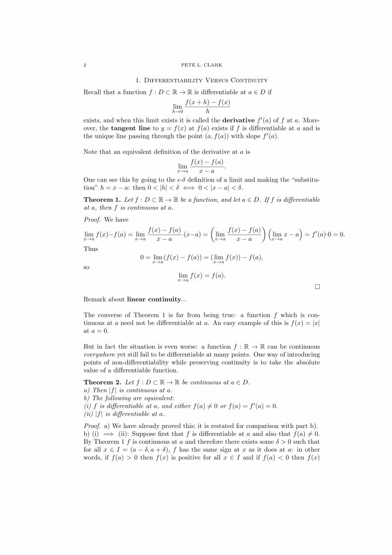
1. Differentiability Versus Continuity

Recall that a function f : D ⊂ R → R is differentiable at a ∈ D if

limh→0

f(x+ h)− f(x)

h

exists, and when this limit exists it is called the derivative f ′(a) of f at a. More-over, the tangent line to y = f(x) at f(a) exists if f is differentiable at a and isthe unique line passing through the point (a, f(a)) with slope f ′(a).

Note that an equivalent definition of the derivative at a is

limx→a

f(x)− f(a)

x− a.

One can see this by going to the ϵ-δ definition of a limit and making the “substitu-tion” h = x− a: then 0 < |h| < δ ⇐⇒ 0 < |x− a| < δ.

Theorem 1. Let f : D ⊂ R → R be a function, and let a ∈ D. If f is differentiableat a, then f is continuous at a.

Proof. We have

limx→a

f(x)−f(a) = limx→a

f(x)− f(a)

x− a·(x−a) =

(limx→a

f(x)− f(a)

x− a

)(limx→a

x− a)= f ′(a)·0 = 0.

Thus

0 = limx→a

(f(x)− f(a)) = ( limx→a

f(x))− f(a),

so

limx→a

f(x) = f(a).

�

Remark about linear continuity...

The converse of Theorem 1 is far from being true: a function f which is con-tinuous at a need not be differentiable at a. An easy example of this is f(x) = |x|at a = 0.

But in fact the situation is even worse: a function f : R → R can be continuouseverywhere yet still fail to be differentiable at many points. One way of introducingpoints of non-differentiability while preserving continuity is to take the absolutevalue of a differentiable function.

Theorem 2. Let f : D ⊂ R → R be continuous at a ∈ D.a) Then |f | is continuous at a.b) The following are equivalent:(i) f is differentiable at a, and either f(a) = 0 or f(a) = f ′(a) = 0.(ii) |f | is differentiable at a.

Proof. a) We have already proved this; it is restated for comparison with part b).b) (i) =⇒ (ii): Suppose first that f is differentiable at a and also that f(a) = 0.By Theorem 1 f is continuous at a and therefore there exists some δ > 0 such thatfor all x ∈ I = (a − δ, a + δ), f has the same sign at x as it does at a: in otherwords, if f(a) > 0 then f(x) is positive for all x ∈ I and if f(a) < 0 then f(x)

MATH 2400 LECTURE NOTES: DIFFERENTIATION 3

is negative for all x ∈ I. In the first case, upon restriction to I, |f | = f , so it isdifferentiable at a since f is. In the second case, upon restriction to I, |f | = −f ,which is also differentiable at a since f is and hence also −f is.

Now suppose that f(a) = f ′(a) = 0 . . .�

2. Differentiation Rules

Theorem 3. (Constant Rule) Let f be differentiable at a ∈ R and C ∈ R. Thenthe function Cf is also differentiable at a and

(Cf)′(a) = Cf ′(a).

Proof. There is nothing to it:

(Cf)′(a) = limh→0

(Cf)(a+ h)− (Cf)(a)

h= C

(limh→0

f(a+ h)− f(a)

h

)= Cf ′(a).

�

Theorem 4. (Sum Rule) Let f and g be functions which are both differentiable ata ∈ R. Then the sum f + g is also differentiable at a and

(f + g)′(a) = f ′(a) + g′(a).

Proof. Again, no biggie:

(f+g)′(a) = limh→0

(f + g)(a+ h)− (f + g)(a)

h= lim

h→0

f(a+ h)− f(a)

h+g(a+ h)− g(a)

h

= limh→0

f(a+ h)− f(a)

h+ lim

h→0

g(a+ h)− g(a)

h= f ′(a) + g′(a).

�

These results, simple as they are, have the following important consequence.

Corollary 5. (Linearity of the Derivative) For any differentiable functions f andg and any constants C1, C2, we have

(C1f + C2g)′ = C1f

′ + C2g′.

The proof is an immediate application of the Sum Rule followed by the ProductRule. The point here is that functions L : V → W with the property that L(v1 +v2) = L(v1) + L(v2) and L(Cv) = CL(v) are called linear mappings, and areextremely important across mathematics.1 The study of linear mappings is thesubject of linear algebra. That differentiation is a linear mapping (on the infinite-dimensional vector space of real functions) provides an important link betweencalculus and algebra.

Theorem 6. (Product Rule) Let f and g be functions which are both differentiableat a ∈ R. Then the product fg is also differentiable at a and

(fg)′(a) = f ′(a)g(a) + f(a)g′(a).

1We are being purposefully vague here as to what sort of things V and W are...

4 PETE L. CLARK

Proof.

(fg)′(a) = limh→0

f(a+ h)g(a+ h)− f(a)g(a)

h

= limh→0

f(a+ h)g(a+ h)− f(a)g(a+ h) + (f(a)g(a+ h)− f(a)g(a))

h

=

(limh→0

f(a+ h)− f(a)

h

)(limh→0

g(a+ h)

)+ f(a)

(limh→0

g(a+ h)− g(a)

h

).

Since g is differentiable at a, g is continuous at a and thus limh→0 g(a + h) =limx→ ag(x) = g(a). The last expression above is therefore equal to

f ′(a)g(a) + f(a)g′(a).

�

Dimensional analysis and the product rule.

The generalized product rule: suppose we want to find the derivative of a func-tion which is a product of not two but three functions whose derivatives we alreadyknow, e.g. f(x) = x sinxex. We can – of course? – still use the product rule, intwo steps:

f ′(x) = (x sinxex)′ = ((x sinx)ex)′ = (x sinx)′ex + (x sinx)(ex)′

= (x′ sinx+ x(sinx)′)ex + x sinxex = sinx+ x cosxex + x sinxex.

Note that we didn’t use the fact that our three differentiable functions were x,sinx and ex until the last step, so the same method shows that for any threefunctions f1, f2, f3 which are all differentiable at x, the product f = f1f2f3 is alsodifferentiable at a and

f ′(a) = f ′1(a)f2(a)f3(a) + f1(a)f

′2(a)f3(a) + f1(a)f2(a)f

′3(a).

Riding this train of thought a bit farther, here a rule for the product of any finitenumber n ≥ 2 of differentiable functions.

Theorem 7. (Generalized Product Rule) Let n ≥ 2 be an integer, and let f1, . . . , fnbe n functions which are all differentiable at a. Then f = f1 · · · fn is also differen-tiable at a, and

(1) (f1 · · · fn)′(a) = f ′1(a)f2(a) · · · fn(a) + . . .+ f1(a) · · · fn−1(a)f

′n(a).

Proof. By induction on n.Base Case (n = 2): This is precisely the “ordinary” Product Rule (Theorem XX).Induction Step: Let n ≥ 2 be an integer, and suppose that the product of any nfunctions which are each differentiable at a ∈ R is differentiable at a and that thederivative is given by (1). Now let f1, . . . , fn, fn+1 be functions, each differentiableat a. Then by the usual product rule

(f1 · · · fnfn+1)′(a) = ((f1 · · · fn)fn+1)

′(a) = (f1 · · · fn)′(a)fn+1(a)+f1(a) · · · fn(a)f ′n+1(a).

Using the induction hypothesis this last expression becomes

(f ′1(a)f2(a) · · · fn(a) + . . .+ f1(a) · · · fn−1(a)f

′n(a)) fn+1(a)+f1(a) · · · fn(a)f ′

n+1(a)

= f ′1(a)f2(a) · · · fn(a)fn+1(a) + . . .+ f1(a) · · · fn(a)f ′

n+1(a).

�

Example: We may use the Generalized Product Rule to give a less computationallyintensive derivation of the power rule

(xn)′ = nxn−1

for n a positive integer. Indeed, taking f1 = · · · = fn = x, we have f(x) = xn =f1 · · · fn, so applying the Generalized Power rule we get

(xn)′ = (x)′x · · ·x+ . . .+ x · · ·x(x)′.Here in each term we have x′ = 1 multipled by n − 1 factors of x, so each termevalutes to xn−1. Moreover we have n terms in all, so

(xn)′ = nxn−1.

No need to mess around with binomial coefficients!Example: More generally, for any differentiable function f and n ∈ Z+, the Gener-alized Product Rule shows that the function f(x)n is differentiable and (f(x)n)′ =nf(x)n−1. (This sort of computation is more traditionally done using the ChainRule...coming up soon!)

Theorem 8. (Quotient Rule) Let f and g be functions which are both differentiable

at a ∈ R, with g(a) = 0. Then fg is differentiable at a and(

f

g

)′

(a) =g(a)f ′(a)− f(a)g′(a)

g(a)2.

Proof. Step 0: First observe that since g is continuous and g(a) = 0, there issome interval I = (a − δ, a + δ) about a on which g is nonzero, and on this

interval fg is defined. Thus it makes sense to consider the difference quotient

f(a+h)/g(a+h)−f(a)/g(a)h for h sufficiently close to zero.

Step 1: We first establish the Reciprocal Rule, i.e., the special case of the Quo-tient Rule in which f(x) = 1 (constant function). Then

(1

g)′(a) = lim

h→0

1/g(a+ h)− 1/g(a)

h

= limh→0

g(a)− g(a+ h)

hg(a)g(a+ h)= −

(limh→0

g(a+ h)− g(a)

h

)(limh→0

1

g(a)g(a+ h)

)=

−g′(a)

g(a)2.

Above we have once again used the fact that g is differentiable at a implies g iscontinuous at a.Step 2: We now derive the full Quotient Rule by combining the Product Rule andthe Reciprocal Rule. Indeed, we have(

f

g

)′

(a) =

(f · 1

g

)′

(a) = f ′(a)1

g(a)+ f(a)

(1

g

)′

(a)

=f ′(a)

g(a)− f(a)

g′(a)

g(a)2=

g(a)f ′(a)− g′(a)f(a)

g(a)2.

�Lemma 9. Let f : D ⊂ R → R. Suppose:(i) limx→a f(x) exists, and(ii) There exists a number L ∈ R such that for all δ > 0, there exists at least one xwith 0 < |x− a| < δ such that f(x) = L.Then limx→a f(x) = L.

6 PETE L. CLARK

Proof. We leave this as an (assigned, this time!) exercise, with the following sugges-tion to the reader: suppose that limx→a f(x) = M = L, and derive a contradictionby taking ϵ to be small enough compared to |M − L|. �Example: Consider, again, for α ∈ R, the function fα : R → R defined by fα(x) =xα sin( 1x ) for x = 0 and fα(0) = 0. Then f satisfies hypothesis (ii) of Lemma 9

with L = 0, since on any deleted interval around zero, the function sin( 1x ) takes thevalue 0 infinitely many times. According to Lemma 9 then, if limx→0 fα(x) existsat all, then it must be 0. As we have seen, the limit exists iff α > 0 and is indeedequal to zero in that case.

Theorem 10. (Chain Rule) Let f and g be functions, and let a ∈ R be such thatf is differentiable at a and g is differentiable at f(a). Then the composite functiong ◦ f is differentiable at a and

(g ◦ f)′(a) = g′(f(a))f ′(a).

Proof. Motivated by Leibniz notation, it is tempting to argue as follows:

(g ◦ f)′(a) = limx→a

g(f(x))− g(f(a))

x− a= lim

x→a

(g(f(x))− g(f(a))

f(x)− f(a)

)·(f(x)− f(a)

x− a

)=

(limx→a

g(f(x))− g(f(a))

f(x)− f(a)

)(limx→a

f(x)− f(a)

x− a

)=

(lim

f(x)→f(a)

g(f(x))− g(f(a))

f(x)− f(a)

)(limx→a

f(x)− f(a)

x− a

)= g′(f(a))f ′(a).

The replacement of “limx→a . . . by limf(x)→f(a) . . .” in the first factor above isjustified by the fact that f is continuous at a.

However, the above argument has a gap in it: when we multiply and divideby f(x) − f(a), how do we know that we are not dividing by zero?? The answeris that we cannot rule this out: it is possible for f(x) to take the value f(a) onarbitarily small deleted intervals around a: again, this is exactly what happens forthe function fα(x) of the above example near a = 0.2 This gap is often held toinvalidate the proof, and thus the most common proof of the Chain Rule in honorscalculus / basic analysis texts proceeds along (superficially, at least) different lines.

But in fact I maintain that the above gap may be rather easily filled to give acomplete proof. The above argument is valid unless the following holds: for allδ > 0, there exists x with 0 < |x− a| < δ such that f(x)− f(a) = 0. So it remainsto give a different proof of the Chain Rule in that case. First, observe that with the

above hypothesis, the difference quotient f(x)−f(a)x−a is equal to 0 at points arbitarily

close to x = a. It follows from Lemma 9 that if

limx→a

f(x)− f(a)

x− a

exists at all, then it must be equal to 0. But we are assuming that the above limitexists, since we are assuming that f is differentiable at a. Therefore what we have

2One should note that in order for a function to have this property it must be “highly oscillatorynear a” as with the functions fα above: indeed, fα is essentially the simplest example of a

function having this kind of behavior. In particular, most of the elementary functions consideredin freshman calculus do not exhibit this highly oscillatory behavior near any point and thereforethe above argument is already a complete proof of the Chain Rule for such functions. Of course

our business here is to prove the Chain Rule for all functions satisfying the hypotheses of thetheorem, even those which are highly oscillatory!

seen is that in the remaining case we have f ′(a) = 0, and therefore, since we aretrying to show that (g◦f)′(a) = g′(f(a))f ′(a), we are trying in this case to show that(g ◦ f)′(a) = 0. So consider our situation: for x ∈ R we have two possibilities: thefirst is f(x)−f(a) = 0, in which case also g(f(x))−g(f(a)) = g(f(a))−g(f(a)) = 0,so the difference quotient is zero at these points. The second is f(x)− f(a) = 0, inwhich case the algebra

g(f(x))− g(f(a)) =g(f(x))− g(f(a))

f(x)− f(a)· f(x)− f(a)

x− a

is justified, and the above argument shows that this expression tends to g′(f(a))f ′(a) =

0 as x → a. So whichever holds, the difference quotient g(f(x))−g(f(a))x−a is close to

(or equal to!) zero.3 Thus the limit tends to zero no matter which alternativeobtains. Somewhat more formally, if we fix ϵ > 0, then the first step of the argu-ment shows that there is δ > 0 such that for all x with 0 < |x − a| < δ such that

f(x) − f(a) = 0, | g(f(x))−g(f(a))x−a | < ϵ. On the other hand, when f(x) − f(a) = 0,

then | g(f(x))−g(f(a))x−a | = 0, so it is certainly less than ϵ! Therefore, all in all we have

0 < |x− a| < δ =⇒ | g(f(x))−g(f(a))x−a | < ϵ, so that

limx→a

g(f(x))− g(f(a))

x− a= 0 = g′(f(a))f ′(a).

�

3. Optimization

3.1. Intervals and interior points.

At this point I wish to digress to formally define the notion of an interval onthe real line and and interior point of the interval. . . .

3.2. Functions increasing or decreasing at a point.

Let f : D → R be a function, and let a be an interior point of D. We say that f isincreasing at a if for all x sufficiently close to a and to the left of a, f(x) < f(a)and for all x sufficiently close to a and to the right of a, f(x) > f(a). More formallyphrased, we require the existence of a δ > 0 such that:• for all x with a− δ < x < a, f(x) < f(a), and• for all x with a < x < a+ δ, f(x) > f(a).

We say f is decreasing at a if there exists δ > 0 such that:• for all x with a− δ < x < a, f(x) > f(a), and• for all x with a < x < a+ δ, f(x) < f(a).

We say f is weakly increasing at a if there exists δ > 0 such that:• for all x with a− δ < x < a, f(x) ≤ f(a), and• for all x with a < x < a+ δ, f(x) ≥ f(a).

3This is the same idea as in the proof of the Switching Theorem, although – to my mild

disappointment – we are not able to simply apply the Switching Theorem directly, since one ofour functions is not defined in a deleted interval around zero.

8 PETE L. CLARK

Exercise: Give the definition of “f is decreasing at a”.

Exercise: Let f : I → R, and let a be an interior point of I.a) Show that f is increasing at a iff −f is decreasing at a.b) Show that f is weakly increasing at a iff −f is weakly decreasing at a.

Example: Let f(x) = mx + b be the general linear function. Then for any a ∈ R:f is increasing at a iff m > 0, f is weakly increasing at a iff m ≥ 0, f is decreasingat a iff m < 0, and f is weakly decreasing at a iff m ≤ 0.

Example: Let n be a positive integer, let f(x) = xn. Then:If x is odd, then for all a ∈ R, f(x) is increasing at a.If x is even, then if a < 0, f(x) is decreasing at a, if a > 0 then f(x) is increasingat a. Note that when n is even f is neither increasing at 0 nor decreasing at 0because for every nonzero x, f(x) > 0 = f(0).4

If one looks back at the previous examples and keeps in mind that we are sup-posed to be studying derivatives (!), one is swiftly led to the following fact.

Theorem 11. Let f : I → R, and let a be an interior point of a. Suppose f isdifferentiable at a.a) If f ′(a) > 0, then f is increasing at a.b) If f ′(a) < 0, then f is decreasing at a.c) If f ′(a) = 0, then no conclusion can be drawn: f may be increasing through a,decreasing at a, or neither.

Proof. a) The differentiability of f at a has an ϵ-δ interpretation, and the idea is touse this interpretation to our advantage. Namely, take ϵ = f ′(a): there exists δ > 0

such that for all x with 0 < |x− a| < δ, | f(x)−f(a)x−a − f ′(a)| < f ′(a), or equivalently

0 <f(x)− f(a)

x− a< 2f ′(a).

In particular, for all x with 0 < |x−a| < δ, f(x)−f(a)x−a > 0, so: if x > a, f(x)−f(a) >

0, i.e., f(x) > f(a); and if x < a, f(x)− f(a) < 0, i.e., f(x) < f(a).b) This is similar enough to part a) to be best left to the reader as an exercise.5

c) If f(x) = x3, then f ′(0) = 0 but f is increasing at 0. If f(x) = −x3, thenf ′(0) = 0 but f is decreasing at 0. If f(x) = x2, then f ′(0) = 0 but f is neitherincreasing nor decreasing at 0. �

3.3. Extreme Values.

Let f : D → R. We say M ∈ R is the maximum value of f on D if(MV1) There exists x ∈ D such that f(x) = M , and(MV2) For all x ∈ D, f(x) ≤ M .

4We do not stop to prove these assertions as it would be inefficient to do so: soon enough wewill develop the right tools to prove stronger assertions. But when given a new definition, it isalways good to find one’s feet by considering some examples and nonexamples of that definition.

5Suggestion: either go through the above proof flipping inequalities as appropriate, or use the

fact that f is decreasing at a iff −f is increasing at a and f ′(a) < 0 ⇐⇒ (−f)′(a) > 0 to applythe result of part a).


It is clear that a function can have at most one maximum value: if it had morethan one, one of the two would be larger than the other! However a function neednot have any maximum value: for instance f : (0,∞) → R by f(x) = 1

x has nomaximum value: limx→0+ f(x) = ∞.

Similarly, we say m ∈ R is the minimum value of f on D if(mV1) There exists x ∈ D such that f(x) = m, and(mV2) For all x ∈ D, f(x) ≥ m.

Again a function clearly can have at most one minimum value but need not haveany at all: the function f : R \ {0} → R by f(x) = 1

x has no minimum value:limx→0− f(x) = −∞.

Exercise: For a function f : D → R, the following are equivalent:(i) f assumes a maximum value M , a minimum value m, and M = m.(ii) f is a constant function.

Recall that a function f : D → R is bounded above if there exists a numberB such that for all x ∈ D, f(x) ≤ B. A function is bounded below if there existsa number b such that for all x ∈ D, f(x) ≥ b. A function is bounded if it is bothbounded above and bounded below: equivalently, there exists B ≥ 0 such that forall x ∈ D, |f(x)| ≤ B: i.e., the graph of f is “trapped between” the horizontal linesy = B and y = −B.

Exercise: Let f : D → R be a function.a) Show: if f has a maximum value, it is bounded above.b) Show: if f has a minimum value, it is bounded below.

Exercise: a) If a function has both a maximum and minimum value on D, then itis bounded on D: indeed, if M is the maximum value of f and m is the minimumvalue, then for all x ∈ B, |f(x)| ≤ max(|m|, |M |).b) Give an example of a bounded function f : R → R which has neither a maximumnor a minimum value.

We say f assumes its maximum value at a if f(a) is the maximum valueof f on D, or in other words, for all x ∈ D, f(x) ≤ f(a). Simlarly, we say fassumes its minimum value at a if f(a) is the minimum value of f on D, or inother words, for all x ∈ D, f(x) ≥ f(a).

Example: The function f(x) = sinx assumes its maximum value at x = π2 , be-

cause sin π2 = 1, and 1 is the maximum value of the sine function. Note however

that π2 is not the only x-value at which f assumes its maximum value: indeed, the

sine function is periodic and takes value 1 precisely at x = π2 + 2πn for n ∈ Z.

Thus there may be more than one x-value at which a function attains its maximumvalue. Similarly f attains its minimum value at x = 3π

2 – f( 3π2 ) = −1 and f takes

no smaller values – and also at x = 3π2 + 2πn for n ∈ Z.

10 PETE L. CLARK

Example: Let f : R → R by f(x) = x3 + 5. Then f does not assume a maxi-mum or minimum value. Indeed, limx→∞ f(x) = ∞ and limx→−∞ f(x) = −∞.

Example: Let f : [0, 2] → R be defined as follows: f(x) = x+ 1, 0 ≤ x < 1.f(x) = 1, x = 1.f(x) = x− 1, 1 < x ≤ 2.Then f is defined on a closed, bounded interval and is bounded above (by 2) andbounded below (by 0) but does not have a maximum or minimum value. Of coursethis example of a function defined on a closed bounded interval without a maximumor minimum value feels rather contrived: in particular it is not continuous at x = 1.

This brings us to the statement (but not yet the proof; sorry!) of one of themost important theorems in this or any course.

Theorem 12. (Extreme Value Theorem) Let f : [a, b] → R be a continuous func-tion. Then f has a maximum and minimum value, and in particular is boundedabove and below.

Again this result is of paramount importance: ubiquitously in (pure and applied)mathematics we wish to optimize functions: that is, find their maximum and orminimum values on a certain domain. Unfortunately, as we have seen above, ageneral function f : D → R need not have a maximum or minimum value! Butthe Extreme Value Theorem gives rather mild hypotheses on which these valuesare guaranteed to exist, and in fact is a useful tool for establishing the existence ofmaximia / minima in other situations as well.

Example: Let f : R → R be defined by f(x) = x2(x − 1)(x − 2). Note that fdoes not have a maximum value: indeed limx→∞ f(x) = limx→−∞ = ∞. However,we claim that f does have a minimum value. We argue for this as follows: giventhat f tends to ∞ with |x|, there must exist ∆ > 0 such that for all x with |x| > ∆,f(x) ≥ 1. On the other hand, if we restrict f to [−∆,∆] we have a continuousfunction on a closed bounded interval, so by the Extreme Value Theorem it musthave a minimum value, say m. In fact since f(0) = 0, we see that m < 0, so inparticular m < 1. This means that the minimum value m for f on [−∆,∆] mustin fact be the minimum value for f on all of R, since at the other values – namely,on (−∞,−∆) and (∆,∞), f(x) > 1 > 0 ≥ m.

We can be at least a little more explicit: a sign analysis of f shows that f ispositive on (−∞, 1) and (2,∞) and negative on (1, 2), so the minimum value of fwill be its minimum value on [1, 2], which will be strictly negative. But exactly whatis this minimum value m, and for which x value(s) does it occur? Stay tuned:weare about to develop tools to answer this question!

3.4. Local Extrema and a Procedure for Optimization.

We now describe a type of “local behavior near a” of a very different sort frombeing increasing or decreasing at a.

Let f : D → R be a function, and let a ∈ D. We say that f has a localmaximum at a if the value of f at a is greater than or equal to its values atall sufficiently close points x. More formally: there exists δ > 0 such that for all

x ∈ D, |x − a| < δ =⇒ f(x) ≤ f(a). Similarly, we say that f has a localminimum at a if the vaalue of f at a is greater than or equal to its values atall sufficiently close points x. More formally: there exists δ > 0 such that for allx ∈ D, |x− a| < δ =⇒ f(x) ≥ f(a).

Theorem 13. Let f : D ⊂ R, and let a be an interior point of a. If f is differ-entiable at a and has a local extremum – i.e., either a local minimum or a localmaximum – at x = a, then f ′(a) = 0.

Proof. Indeed, if f ′(a) = 0 then either f ′(a) > 0 or f ′(a) < 0.If f ′(a) > 0, then by Theorem X.X f is increasing at a. Thus for x slightly smallerthan a, f(x) < f(a), and for x slightly larger than a, f(x) > f(a). So f does nothave a local extremum at a.Similarly, if f ′(a) < 0, then by Theorem X.X f is decreasing at a. Thus for xslightly smaller than a, f(x) > f(a), and for x slightly larger than a, f(x) < f(a).So f does not have a local extremum at a. �

Theorem 14. (Optimization Procedure) Let f : [a, b] → R be continuous. Thenthe minimum and maximum values must each be attained at a point x ∈ [a, b] whichis either:(i) an endpoint: x = a or x = b,(ii) a stationary point: f ′(a) = 0, or(iii) a point of nondifferentiability.

Often one lumps cases (ii) and (iii) of Theorem XX together under the term crit-ical point (but there is nothing very deep going on here: it’s just terminology).Clearly there are always exactly two endpoints. In favorable circustances therewill be only finitely many critical points, and in very favorable circumstances theycan be found exactly: suppose they are c1, . . . , cn. (There may in fact not be anycritical points, but that would only make our discussion easier...) Suppose furtherthat we can explicitly compute all the values f(a), f(b), f(c1), . . . , f(cn). Then wewin: the largest of these values is the maximum value, and the minimum of thesevalues is the minimum value.

Example: Let f(x) = x2(x − 1)(x − 2) = x4 − 3x3 + 2x2. Above we arguedthat there is a ∆ such that |x| > ∆ =⇒ |f(x)| ≥ 1: let’s find such a ∆ explicitly.We intend nothing fancy here:

f(x) = x4 − 3x2 + 2x2 ≥ x4 − 3x3 = x3(x− 3).

So if x ≥ 4, then

x3(x− 3) ≥ 43 · 1 = 64 ≥ 1.

On the other hand, if x < −1, then x < 0, so −3x3 > 0 and thus

f(x) ≥ x4 + 2x2 = x2(x2 + 2) ≥ 1 · 3 = 3.

Thus we may take ∆ = 4. Now let us try the procedure of Theorem XX out byfinding the maximim and minimum values of f(x) = x4 − 3x3 + 2x2 on [−4, 4].

Since f is differentiable everywhere on (−4, 4), the only critical points will be thestationary points, where f ′(x) = 0. So we compute the derivative:

f ′(x) = 4x3 − 9x2 + 4x = x(4x2 − 9x+ 4).

12 PETE L. CLARK

The roots are x = 9±√17

8 , or, approximately,

x1 ≈ 0.6094 . . . , x2 = 1.604 . . . .

f(x1) = 0.2017 . . . , f(x2) = −0.619 . . . .

Also we always test the endpoints:

f(−4) = 480, f(4) = 96.

So the maximum value is 480 and the minimum value is −.619 . . ., occurring at9+

√17

8 .

3.5. Remarks on finding roots of f ′.

4. The Mean Value Theorem

4.1. Statement of the Mean Value Theorem.

Our goal in this section is to prove the following important result.

Theorem 15. (Mean Value Theorem) Let f : [a, b] → R be continuous on [a, b]and differentiable on (a, b). Then there exists at least one c such that a < c < b and

f ′(c) =f(b)− f(a)

b− a.

Remark: If you will excuse a (vaguely) personal anecdote: I still remember thecalculus test I took in high school in which I was asked to state the Mean ValueTheorem. It was a multiple choice question, and I didn’t see the choice I wanted,which was as above except with the subtly stronger assumption that f ′

R(a) andf ′L(b) exist: i.e., f is one-sided differentiable at both endpoints. So I went up to theteacher’s desk to ask about this. He thought for a moment and said, “Okay, youcan add that as an answer if you want”, and so as not to give special treatment toany one student, he announced to the class that he was adding a possible answer tothe Mean Value Theorem question. So I marked my added answer, did the rest ofthe exam, and then had time to come back to this question. Upon further reflectionit became clear that one-sided differentiability at the endpoints was not in fact re-quired, i.e., one of the pre-existing choices was the correct answer and not the one Ihad added. So I changed my answer and submitted my exam. As you can see fromthe statement above, my final answer was correct. But many students in the classfigured that if I had successfully lobbied for an additional answer then this answerwas probably the correct one, with the effect that they changed their answer fromthe correct answer to my incorrect added answer! They were not so thrilled witheither me or the teacher, but in my opinion he at least behaved admirably: thiswas a real “teachable moment”!

One should certainly draw a picture to go with the Mean Value Theorem, as ithas a very simple geometric interpretation: under the hypotheses of the theorem,there exists at least one interior point c of the interval such that the tangent lineat c is parallel to the secant line joining the endpoints of the interval.

And one should also interpret it physically: if y = f(x) gives the position of a

particle at a given time x, then the expression f(b)−f(a)b−a is nothing less than the

average velocity between time a and time b, whereas the derivative f ′(c) is the in-stantaneous velocity at time c, so that the Mean Value Theorem says that there is at

least one instant at which the instantaneous velocity is equal to the average velocity.

Example: Suppose that cameras are set up at certain checkpoints along an in-terstate highway in Georgia. One day you receive in the mail photos of yourselfat two checkpoints. The two checkpoints are 90 miles apart and the second photois taken 73 minutes after the first photo. You are issued a ticket for violating thespeeed limit of 70 miles per hour. The enclosed letter explains: your average veloc-ity was (90 miles) / (73 minutes) · (60 minutes) / (hour) ≈ 73.94 miles per hour.Thus, although no one saw you violating the speed limit, they may mathematicallydeduce that at some point your instantaneous velocity was over 70 mph. Guilt bythe Mean Value Theorem!

4.2. Proof of the Mean Value Theorem.

We will deduce the Mean Value Theorem from the Extreme Value Theorem (whichwe have not yet proven, but all in good time...). However, it is convenient to firstestablish a special case.

Theorem 16. (Rolle’s Theorem) Let f : [a, b] → R. We suppose:(i) f is continuous on [a, b].(ii) f is differentiable on (a, b).(iii) f(a) = f(b).Then there exists c with a < c f(a) = f(b). Then the maximum value does not occurat either endpoint. Since f is differentiable on (a, b), it must therefore occur at astationary point: i.e., there exists c ∈ (a, b) with f ′(c) = 0.Case 2: Suppose m < f(a) = f(b). Then the minimum value does not occur ateither endpoint. Since f is differentiable on (a, b), it must therefore occur at astationary point: there exists c ∈ (a, b) with f ′(c) = 0.Case 3: The remaining case is f(a) ≤ m ≤ M ≤ f(a), which implies m = M =f(a) = f(b), so f is constant. In this case f ′(c) = 0 at every point c ∈ (a, b)! �

To deduce the Mean Value Theorem from Rolle’s Theorem, it is tempting to tiltour head until the secant line from (a, f(a)) to (b, f(b)) becomes horizontal andthen apply Rolle’s Theorem. The possible flaw here is that if we start a subset inthe plane which is the graph of a function and rotate it too much, it may no longerbe the graph of a function, so Rolle’s Theorem does not apply.

The above objection is just a technicality. In fact, it suggests that more is true:there should be some version of the Mean Value Theorem which applies to curvesin the plane which are not necessarily graphs of functions. Indeed we will meetsuch a generalization later – the Cauchy Mean Value Theorem – and use itto prove L’Hopital’s Rule – but at the moment it is, alas, easier to use a simple trick.

Proof of the Mean Value Theorem: Let f : [a, b] → R be continuous on [a, b] anddifferentiable on (a, b). There is a unique linear function L(x) such that L(a) = f(a)and L(b) = f(b): indeed, L is nothing else than the secant line to f between (a, f(a))and (b, f(b)). Here’s the trick: by subtracting L(x) from f(x) we reduce ourselvesto a situation where we may apply Rolle’s Theorem, and then the conclusion that

14 PETE L. CLARK

we get is easily seen to be the one we want about f .Here goes: define

g(x) = f(x)− L(x).

Then g is defined and continuous on [a, b], differentiable on (a, b), and g(a) =f(a)−L(a) = f(a)−f(a) = 0 = f(b)−f(b) = f(b)−L(b) = g(b). Applying Rolle’sTheorem to g, there exists c ∈ (a, b) such that g′(c) = 0. On the other hand, since

L is a linear function with slope f(b)−f(a)b−a , we compute

0 = g′(c) = f ′(c)− L′(c) = f ′(c)− f(b)− f(a)

b− a,

and thus

f ′(c) =f(b)− f(a)

b− a.

4.3. The Cauchy Mean Value Theorem.

We present here a modest generalization of the Mean Value Theorem due to A.L.Cauchy. Although perhaps not as fundamental and physically appealing as theMean Value Theorem, it certainly has its place: for instance it may be used toprove L’Hopital’s Rule.

Theorem 17. (Cauchy Mean Value Theorem) Let f, g : [a, b] → R be continuousand differentiable on (a, b). Then there exists c ∈ (a, b) such that

(2) (f(b)− f(a))g′(c) = (g(b)− g(a))f ′(c).

Proof. Case 1: Suppose g(a) = g(b). By Rolle’s Theorem, there is c ∈ (a, b) suchthat g′(c) = 0. With this value of c, both sides of (2) are zero, hence they are equal.Case 2: Suppose g(a) = g(b), and define

h(x) = f(x)−(f(b)− f(a)

g(b)− g(a)

)g(x).

Then h is continuous on [a, b], differentiable on (a, b), and

h(a) =f(a)(g(b)− g(a))− g(a)(f(b)− f(a))

g(b)− g(a)=

f(a)g(b)− g(a)f(b)

g(b)− g(a),

h(b) =f(b)(g(b)− g(a))− g(b)(f(b)− f(a))

g(b)− g(a)=

f(a)g(b)− g(a)f(b)

g(b)− g(a),

so h(a) = h(b).6 By Rolle’s Theorem there exists c ∈ (a, b) with

0 = h′(c) = f ′(c)−(f(b)− f(a)

g(b)− g(a)

)g′(c),

or equivalently,

(f(b)− f(a))g′(c) = (g(b)− g(a))f ′(c).

�

Exercise: Which choice of g recovers the “ordinary” Mean Value Theorem?

6Don’t be so impressed: we wanted a constant C such that if h(x) = f(x) − Cg(x), thenh(a) = h(b), so we set f(a)− Cg(a) = f(b)− Cg(b) and solved for C.

5. Monotone Functions

5.1. The Monotone Function Theorems.

The Mean Value Theorem has several important consequences. Foremost of allit will be used in the proof of the Fundamental Theorem of Calculus, but that’s forlater. At the moment we can use it to establish a criterion for a function f to beincreasing / weakly increasing / decreasing / weakly decreasing on an interval interms of sign condition on f ′.

Theorem 18. (First Monotone Function Theorem) Let I be an open interval, andlet f : I → R be a function which is differentiable on I.a) Suppose f ′(x) > 0 for all x ∈ I. Then f is increasing on I: for all x1, x2 ∈ Iwith x1 < x2, f(x1) < f(x2).b) Suppose f ′(x) ≥ 0 for all x ∈ I. Then f is weakly increasing on I: for allx1, x2 ∈ I with x1 < x2, f(x1) ≤ f(x2).c) Suppose f ′(x) < 0 for all x ∈ I. Then f is decreasing on I: for all x1, x2 inIwith x1 < x2, f(x1) > f(x2).d) Suppose f ′(x) ≤ 0 for all x ∈ I. Then f is weakly decreasing on I: for allx1, x2 ∈ I with x1 < x2, f(x1) ≥ f(x2).

Proof. a) We go by contraposition: suppose that f is not increasing: then thereexist x1, x2 ∈ I with x1 < x2 such that f(x1) ≥ f(x2). Apply the Mean Value

Theorem to f on [x1, x2]: there exists x1 < c < x2 such that f ′(c) = f(x2)−f(x1)x2−x1

≤ 0.

b) Again, we argue by contraposition: suppose that f is not weakly increasing: thenthere exist x1, x2 ∈ I with x1 < x2 such that f(x1) > f(x2). Apply the Mean Value

Theorem to f on [x1, x2]: there exists x1 < c < x2 such that f ′(c) = f(x2)−f(x1)x2−x1

< 0.

c),d) We leave these proofs to the reader. One may either proceed exactly as inparts a) and b), or reduce to them by multiplying f by −1. �Corollary 19. (Zero Velocity Theorem) Let f : I → R be a differentiable functionwith identically zero derivative. Then f is constant.

Proof. Since f ′(x) ≥ 0 for all x ∈ I, f is weakly increasing on I: x1 < x2 =⇒f(x1) ≤ f(x2). Since f ′(x) ≤ 0 for all x ∈ I, f is weakly decreasing on I: x1 <x2 =⇒ f(x1) ≥ f(x2). But a function which is weakly increasing and weaklydecreasing satsifies: for all x1 < x2, f(x1) ≤ f(x2) and f(x1) ≥ f(x2) and thusf(x1) = f(x2): f is constant. �Remark: The strategy of the above proof is to deduce Corollary 19 from the In-creasing Function Theorem. In fact if we argued directly from the Mean ValueTheorem the proof would be significantly shorter: try it!

Corollary 20. Suppose f, g : I → R are both differentiable and such that f ′ = g′

(equality as functions, i.e., f ′(x) = g′(x) for all x ∈ I). Then there exists a constantC ∈ R such that f = g + C, i.e., for all x ∈ I, f(x) = g(x) + C.

Proof. Let h = f − g. Then h′ = (f − g)′ = f ′ − g′ ≡ 0, so by Corollary 19, h ≡ Cand thus f = g + h = g + C. �Remark: Corollary 20 can be viewed as the first “uniqueness theorem” for differen-tial equations. Namely, suppose that f : I → R is some function, and consider theset of all functions F : I → R such that F ′ = f . Then Corollary ?? asserts that if

16 PETE L. CLARK

there is a function F such that F ′ = f , then there is a one-parameter family ofsuch functions, and more specifically that the general such function is of the formF +C. In perhaps more familiar terms, this asserts that antiderivatives are uniqueup to an additive constant, when they exist.

On the other hand, the existence question lies deeper: namely, given f : I → R,must there exist F : I → R such that F ′ = f? In general the answer is no.

Exercise: Let f : R → R by f(x) = 0 for x ≤ 0 and f(x) = 1 for x > 0. Show thatthere is no function F : R → R such that F ′ = f .

In other words, not every function f : R → R has an antiderivative, i.e., isthe derivative of some other function. It turns out that every continuous functionhas an antiderivative: this will be proved in the second half of the course. (On thethird hand, there are some discontinuous functions which have antiderivatives, butit is too soon to get into this...)

Corollary 21. Let n ∈ Z+, and let f : I → R be a function whose nth derivativef (n) is identically zero. Then f is a polynomial function of degree at most n− 1.

Proof. Exercise. (Hint: use induction.) �The setting of the Increasing Function Theorem is that of a differentiable functiondefined on an open interval I. This is just a technical convenience: for continu-ous functions, the increasing / decreasing / weakly increasing / weakly decreasingbehavior on the interior of I implies the same behavior at an endpoint of I.

Theorem 22. Let f : [a, b] → R be a function. We suppose:(i) f is continuous at x = a and x = b.(ii) f is weakly increasing (resp. increasing, weakly decreasing, decreasing) on(a, b).Then f is weakly increasing (resp. increasing, weakly decreasing, decreasing) on[a, b].

Remark: The “resp.” in the statement above is an abbreviation for “respectively”.Use of respectively in this way is a shorthand way for writing out several cognatestatements. In other words, we really should have four different statements, eachone of the form “if f has property X on (a, b), then it also has property X on[a, b]”, where X runs through weakly increasing, increasing, weakly decreasing, anddecreasing. Use of “resp.” in this way is not great mathematical writing, but it issometimes seen as preferable to the tedium of writing out a large number of verysimilar statements. It certainly occurs often enough for you to get used to seeingand understanding it.

Proof. There are many similar statements here; let’s prove some of them.Step 1: Suppose that f is continuous at a and weakly increasing on (a, b). Wewill show that f is weakly increasing on [a, b). Indeed, assume not: then thereexists x0 ∈ (a, b) such that f(a) > f(x0). Now take ϵ = f(a) − f(x0); since fis (right-)continuous at a, there exists δ > 0 such that for all a ≤ x < a + δ,|f(x) − f(a)| < f(a) − f(x0), which implies f(x) > f(x0). By taking a < x < x0,this contradicts the assumption that f is weakly increasing on (a, b).Step 2: Suppose that f is continuous at a and increasing on (a, b). We will show

that f is increasing on [a, b). Note first that Step 1 applies to show that f(a) ≤ f(x)for all x ∈ (a, b), but we want slightly more than this, namely strict inequality. So,seeking a contradiction, we suppose that f(a) = f(x0) for some x0 ∈ (a, b). Butnow take x1 ∈ (a, x0): since f is increasing on (a, b) we have f(x1) < f(x0) = f(a),contradicting the fact that f is weakly increasing on [a, b).Step 3: In a similar way one can handle the right endpoint b. Now suppose thatf is increasing on [a, b) and also increasing on (a, b]. It remains to show that f isincreasing on [a, b]. The only thing that could go wrong is f(a) ≥ f(b). To see thatthis cannot happen, choose any c ∈ (a, b): then f(a) < f(c) < f(b). �

Let us say that a function f : I → R is monotone if it is either increasing onI or decreasing on I, and also that f is weakly monotone if it is either weaklyincreasing on I or weakly decreasing on I.

Theorem 23. (Second Monotone Function Theorem) Let f : I → R be a functionwhich is continuous on I and differentiable on the interior I◦ of I (i.e., at everypoint of I except possibly at any endpoints I may have).a) The following are equivalent:(i) f is weakly monotone.(ii) Either we have f ′(x) ≥ 0 for all x ∈ I◦ or f ′(x) ≤ 0 for all x ∈ I◦.b) Suppose f is weakly monotone. The following are equivalent:(i) f is not monotone.(ii) There exist a, b ∈ I◦ with a < b such that the restriction of f to [a, b is constant.(iii) There exist a, b ∈ I◦ with a < b such that f ′(x) = 0 for all x ∈ [a, b].

Proof. Throughout the proof we restrict our attention to increasing / weakly in-creasing functions, leaving the other case to the reader as a routine exercise.a) (i) =⇒ (ii): Suppose f is weakly increasing on I. We claim f ′(x) ≥ 0 for allx ∈ I◦. If not, there is a ∈ I◦ with f ′(a) < 0. Then f is decreasing at a, so thereexists b > a with f(b) < f(a), contradicting the fact that f is weakly decreasing.(ii) =⇒ (i): Immediate from the Increasing Function Theorem and Theorem 22.b) (i) =⇒ (ii): Suppose f is weakly increasing on I but not increasing on I. ByTheorem 22 f is still not increasing on I◦, so there exist a, b ∈ I◦ with a < b suchthat f(a) = f(b). Then, since f is weakly increasing, for all c ∈ [a, b] we havef(a) ≤ f(c) ≤ f(b) = f(a), so f is constant on [a, b].(ii) =⇒ (iii): If f is constant on [a, b], f ′ is identically zero on [a, b].(iii) =⇒ (i): If f ′ is identically zero on some subinterval [a, b], then by the ZeroVelocity Theorem f is constant on [a, b], hence is not increasing. �

The next result follows immediately.

Corollary 24. Let f : I → R be differentiable. Suppose that f ′(x) ≥ 0 for allx ∈ I, and that f ′(x) > 0 except at a finite set of points x1, . . . , xn. Then f isincreasing on I.

Example: A typical application of Theorem 24 is to show that the function f :R → R by f(x) = x3 is increasing on all of R. Indeed, f ′(x) = 3x2 which is strictlypositive at all x = 0 and 0 at x = 0.

5.2. The First Derivative Test.

We can use Theorem 22 to quickly derive another staple of freshman calculus.

18 PETE L. CLARK

Theorem 25. (First Derivative Test) Let I be an interval, a an interior point of I,and f : I → R a function. We suppose that f is continuous on I and differentiableon I \ {a} – i.e., differentiable at every point of I except possibly at x = a. Then:a) If there exists δ > 0 such that f ′(x) is negative on (a − δ, a) and is positive on(a, a+ δ). Then f has a strict local minimum at a.b) If there exists δ > 0 such that f ′(x) is positive on (a − δ, a) and is negative on(a, a+ δ). Then f has a strict local maximum at a.

Proof. a) By the First Monotone Function Theorem, since f ′ is negative on theopen interval (a− δ, a) and positive on the open interval (a, a+ δ) f is decreasingon (a− δ, a) and increasing on (a, a+ δ). Moreover, since f is differentiable on itsentire domain, it is continuous at a− δ, a and a+ δ, and thus Theorem 22 appliesto show that f is decreasing on [a − δ, a] and increasing on [a, a + δ]. This givesthe desired result, since it implies that f(a) is strictly smaller than f(x) for anyx ∈ [a− δ, a) or in (a, a+ δ].b) As usual this may be proved either by revisiting the above argument or deduceddirectly from the result of part a) by multiplying f by −1. �

Remark: This version of the First Derivative Test is a little stronger than thefamiliar one from freshman calculus in that we have not assumed that f ′(a) = 0nor even that f is differentiable at a. Thus for instance our version of the testapplies to f(x) = |x| to show that it has a strict local minimum at x = 0.

5.3. The Second Derivative Test.

Theorem 26. (Second Derivative Test) Let a be an interior point of an intervalI, and let f : I → R. We suppose:(i) f is twice differentiable at a, and(ii) f ′(a) = 0.Then if f ′′(a) > 0, f has a strict local minimum at a, whereas if f ′′(a) < 0, f hasa strict local maximum at a.

Proof. As usual it suffices to handle the case f ′′(a) > a.Notice that the hypothesis that f is twice differentiable at a implies that f isdifferentiable on some interval (a−δ, a+δ) ( otherwise it would not be meaningful totalk about the derivative of f ′ at a). Our strategy will be to show that for sufficientlysmall δ > 0, f ′(x) is negative for x ∈ (a − δ, a) and positive for x ∈ (a, a + δ) andthen apply the First Derivative Test. To see this, consider

f ′′(a) = limx→a

f ′(x)− f ′(a)

x− a= lim

x→a

f ′(x)

x− a.

We are assuming that this limit exists and is positive, so that there exists δ > 0

such that for all x ∈ (a−δ, a)∪(a, a+δ), f ′(x)x−a is positive. And this gives us exactly

what we want: suppose x ∈ (a− δ, a). Then f ′(x)x−a > 0 and x− a < 0, so f ′(x) < 0.

On the other hand, suppose x ∈ (a, a + δ). Then f ′(x)x−a > 0 and x − a > 0, so

f ′(x) > 0. So f has a strict local minimum at a by the First Derivative Test. �

Remark: When f ′(a) = f ′′(a) = 0, no conclusion can be drawn about the localbehavior of f at a: it may have a local minimum at a, a local maximum at a, beincreasing at a, decreasing at a, or none of the above.

5.4. Sign analysis and graphing.

When one is graphing a function f , the features of interest include number andapproximate locations of the roots of f , regions on which f is positive or negative,regions on which f is increasing or decreasing, and local extrema, if any. For theseconsiderations one wishes to do a sign analysis on both f and its derivative f ′.

Let us agree that a sign analysis of a function g : I → R is the determina-tion of regions on which g is positive, negative and zero.

The basic strategy is to determine first the set of roots of g. As discussed before,finding exact values of roots may be difficult or impossible even for polynomialfunctions, but often it is feasible to determine at least the number of roots andtheir approximate location (certainly this is possible for all polynomial functions,although this requires justification that we do not give here). The next step is totest a point in each region between consecutive roots to determine the sign.

This procedure comes with two implicit assumptions. Let us make them explicit.

The first is that the roots of f are sparse enough to separate the domain I into“regions”. One precise formulation of of this is that f has only finitely many rootson any bounded subset of its domain. This holds for all the elementary functions weknow and love, but certainly not for all functions, even all differentiable functions:we have seen that things like x2 sin( 1x ) are not so well-behaved. But this is a con-venient assumption and in a given situation it is usually easy to see whether it holds.

The second assumption is more subtle: it is that if a function f takes a posi-tive value at some point a and a negative value at some other point b then it musttake the value zero somewhere in between. Of course this does not hold for allfunctions: it fails very badly, for instance, for the function f which takes the value1 at every rational number and −1 at every irrational number.

Let us formalize the desired property and then say which functions satisfy it.

A function f : I → R has the intermediate value property if for all a, b ∈ Iwith a < b and all L in between f(a) and f(b) – i.e., with f(a) < L < f(b) orf(b) < L < f(a) – there exists some c ∈ (a, b) with f(c) = L.

Thus a function has the intermediate value property when it does not “skip” values.

Here are two important theorems, each asserting that a broad class of functionshas the intermediate value property.

Theorem 27. (Intermediate Value Theorem) Let f : [a, b] → R be a continuousfunction defined on a closed, bounded interval. Then f has the intermediate valueproperty.

Example of a continuous function f : [0, 2]Q → Q failing the intermediate value

property. Let f(x) be −1 for 0 ≤ x <√2 and f(x) = 1 for

√2 < x ≤ 1.

20 PETE L. CLARK

The point of this example is to drive home the point that the Intermediate ValueTheorem is the second of our three “hard theorems” in the sense that we have nochance to prove it without using special properties of the real numbers beyond theordered field axioms. And indeed we will not prove IVT right now, but we will useit, just as we used but did not yet prove the Extreme Value Theorem. (However weare now not so far away from the point at which we will “switch back”, talk aboutcompleteness of the real numbers, and prove the three hard theorems.)

The Intermediate Value Theorem (or IVT) is ubiquitously useful. As alluded toearlier, even such innocuous properties as every non-negative real number having asquare root contain an implicit appeal to IVT. From the present point of view, itjustifies the following observation.

Let f : I → R be a continuous function, and suppose that there are only finitelymany roots, i.e., there are x1, . . . , xn ∈ I such that f(xi) = 0 for all i and f(x) = 0for all other x ∈ I. Then I \ {x1, . . . , xn} is a finite union of intervals, and on eachof them f has constant sign: it is either always positive or always negative.

So this is how sign analysis works for a function f when f is continuous – a verymild assumption. But as above we also want to do a sign analysis of the derivativef ′: how may we justify this?

Well, here is one very reasonable justification: if the derivative f ′ of f is itselfcontinuous, then by IVT it too has the intermediate value property and thus, atleast if f ′ has only finitely many roots on any bounded interval, sign analysis isjustified. This brings up the following basic question.

Question 1. Let f : I → R be a differentiable function? Must its derivativef ′ : I → R be continuous?

Let us first pause to appreciate the subtlety of the question: we are not askingwhether f differentiable implies f continuous: we proved long ago and have usedmany times that this is the case. Rather we are asking whether the new functionf ′ can exist at every point of I but fail to itself be a continuous function. In factthe answer is yes.

Example: Let f(x) = x2 sin( 1x ). I claim that f is differentiable on all of R butthat the derivative is discontinuous at x = 0, and in fact that limx→0 f

′(x) doesnot exist. . . .

Theorem 28. (Darboux) Let f : I → R be a differentiable function. Supposethat we have a, b ∈ I with a < b and f ′(a) < f ′(b). Then for every L ∈ R withf ′(a) < L < f ′(b), there exists c ∈ (a, b) such that f ′(c) = L.

Proof. Step 1: First we handle the special case L = 0, which implies f ′(a) < 0 andf ′(b) > 0. Now f is a differentiable – hence continuous – function defined on theclosed interval [a, b] so assumes its minimum value at some point c ∈ [a, b]. If c isan interior point, then as we have seen, it must be a stationary point: f ′(c) = 0.But the hypotheses guarantee this: since f ′(a) < 0, f is decreasing at a, thustakes smaller values slightly to the right of a, so the minimum cannot occur at a.Similarly, since f ′(b) > 0, f is increasing at b, thus takes smaller values slightly to

the left of b, so the minimum cannot occur at b.Step 2: We now reduce the general case to the special case of Step 1 by definingg(x) = f(x)− Lx. Then g is still differentiable, g′(a) = f ′(a)− L < 0 and g′(b) =f ′(b)− L > 0, so by Step 1, there exists c ∈ (a, b) such that 0 = g′(c) = f ′(c)− L.In other words, there exists c ∈ (a, b) such that f ′(c) = L. �

Remark: Of course there is a corresponding version of the theorem when f(b) <L < f(a). Darboux’s Theorem also often called the Intermediate Value The-orem For Derivatives, terminology we will understand better when we discussthe Intermediate Value Theorem (for arbitrary continuous functions).

Exercise: Let a be an interior point of an interval I, and suppose f : I → R isa differentiable function. Show that the function f ′ cannot have a simple dis-continuity at x = a. (Recall that a function g has a simple discontinuity at aif limx→a− g(x) and limx→a+ g(x) both exist but either they are unequal to eachother or they are unequal to g(a).)

5.5. A theorem of Spivak.

The following theorem is taken directly from Spivak’s book (Theorem 7 of Chapter11): it does not seem to be nearly as well known as Darboux’s Theorem (and infact I think I encountered it for the first time in Spivak’s book).

Theorem 29. Let a be an interior point of I, and let f : I → R. Suppose:(i) f is continuous on I,(ii) f is differentiable on I \ {a}, i.e., at every point of I except possibly at a, and(iii) limx→a f

′(x) = L exists.Then f is differentiable at a and f ′(a) = L.

Proof. Choose δ > 0 such that (a − δ, a + δ) ⊂ I. Let x ∈ (a, a + δ). Then f isdifferentiable at x, and we may apply the Mean Value Theorem to f on [a, x]: thereexists cx ∈ (a, x) such that

f(x)− f(a)

x− a= f ′(cx).

Now, as x → a every point in the interval [a, x] gets arbitrarily close to x, solimx→a cx = x and thus

f ′R(a) = lim

x→a+

f(x)− f(a)

x− a= lim

x→a+f ′(cx) = lim

x→a+f ′(x) = L.

By a similar argument involving x ∈ (a− δ, a) we get

f ′L(a) = lim

x→f ′(x) = L,

so f is differentiable at a and f ′(a) = L. �

6. Inverse Functions I: Theory

6.1. Review of inverse functions.

Let X and Y be sets, and let f : X → Y be a function between them. Recallthat an inverse function is a function g : Y → X such that

g ◦ f = 1X : X → X, f ◦ g = 1Y : Y → Y.

22 PETE L. CLARK

Let’s unpack this notation: it means the following: first, that for all x ∈ X, (g ◦f)(x) = g(f(x)) = x; and second, that for all y ∈ Y , (f ◦ g)(y) = f(g(y)) = y.

Proposition 30. (Uniqueness of Inverse Functions) Let f : X → Y be a function.Suppose that g1, g2 : Y → X are both inverses of f . Then g1 = g2.

Proof. For all y ∈ Y , we have

g1(y) = (g2 ◦ f)(g1(y)) = g2(f(g1(y))) = g1(y).

�

Since the inverse function to f is always unique provided it exists, we denote it byf−1. (Caution: In general this has nothing to do with 1

f . Thus sin−1(x) = csc(x) =

1sin x . Because this is legitimately confusing, many calculus texts write the inverse

sine function as arcsinx. But in general one needs to get used to f−1 being usedfor the inverse function.)

We now turn to giving conditions for the existence of the inverse function. Re-call that f : X → Y is injective if for all x1, x2 ∈ X, x1 = x2 =⇒ f(x1) = f(x2).In other words, distinct x-values get mapped to distinct y-values. (And in yet otherwords, the graph of f satisfies the horizontal line test.) Also f : X → Y is surjec-tive if for all y ∈ Y , there exists at least one x ∈ X such that y = f(x).

Putting these two concepts together we get the important notion of a bijectivefunction f : X → Y , i.e., a function which is both injective and surjective. Other-wise put, for all y ∈ Y there exists exactly one x ∈ X such that y = f(x). It maywell be intuitively clear that bijectivity is exactly the condition needed to guaranteeexistence of the inverse function: if f is bijective, we define f−1(y) = xy, the uniqueelement of X such that f(xy) = y. And if f is not bijective, this definition breaksdown and thus we are unable to define f−1. Nevertheless we ask the reader to bearwith us as we give a slightly tedious formal proof of this.

Theorem 31. (Existence of Inverse Functions) For f : X → Y , TFAE:(i) f is bijective.(ii) f admits an inverse function.

Proof. (i) =⇒ (ii): If f is bijective, then as above, for each y ∈ X there existsexactly one element of X – say xy – such that f(xy) = y. We may therefore define afunction g : Y → X by g(y) = xy. Let us verify that g is in fact the inverse functionof f . For any x ∈ X, consider g(f(x)). Because f is injective, the only elementx′ ∈ X such that f(x′) = f(x) is x′ = x, and thus g(f(x)) = x. For any y ∈ Y , letxy be the unique element of X such that f(xy) = y. Then f(g(y)) = f(xy) = y.(ii) =⇒ (i): Suppose that f−1 exists. To see that f is injective, let x1, x2 ∈ Xbe such that f(x1) = f(x2). Applying f−1 on the left gives x1 = f−1(f(x1)) =f−1(f(x2)) = x2. So f is injective. To see that f is surjective, let y ∈ Y . Thenf(f−1(y)) = y, so there is x ∈ X with f(x) = y, namely x = f−1(y). �

For any function f : X → Y , we define the image of f to be {y ∈ Y | ∃x ∈ X | y =f(x)}. The image of f is often denoted f(X).7

7This is sometimes called the range of f , but sometimes not. It is safer to call it the image!


We now introduce the dirty trick of codomain restriction. Let f : X → Ybe any function. Then if we replace the codomain Y by the image f(X), we stillget a well-defined function f : X → f(X), and this new function is tautologicallysurjective. (Imagine that you manage the up-and-coming band Yellow Pigs. Youget them a gig one night in an enormous room filled with folding chairs. Aftereveryone sits down you remove all the empty chairs, and the next morning youwrite a press release saying that Yellow Pigs played to a “packed house”. This isessentially the same dirty trick as codomain restriction.)

Example: Let f : R → R by f(x) = x2. Then f(R) = [0,∞), and althoughx2 : R → R is not surjective, x2 : R → [0,∞) certainly is.

Since a codomain-restricted function is always surjective, it has an inverse iff itis injective iff the original functionb is injective. Thus:

Corollary 32. For a function f : X → Y , the following are equivalent:(i) The codomain-restricted function f : X → f(X) has an inverse function.(ii) The original function f is injective.

6.2. The Interval Image Theorem.

Next we want to return to earth by considering functions f : I → R and theirinverses, concentrating on the case in which f is continuous.

Theorem 33. (Interval Image Theorem) Let I ⊂ R be an interval, and let f : I →R be a continuous function. Then the image f(I) of f is also an interval.

Proof. At the moment we will give the proof only when I = [a, b], i.e., is closedand bounded. The general case will be discussed later when we switchback to talkabout least upper bounds. Now suppose f : [a, b] → R is continuous. Then f has aminimum value m, say at xm and a maximum value M , say at xM . It follows thatthe image f([a, b]) of f is a subset of the interval [m,M ]. Moreover, if L ∈ (m,M),then by the Intermediate Value Theorem there exists c in between xm and xM suchthat f(c) = L. So f([a, b]) = [m,M ]. �

Remark: Although we proved only a special case of the Interval Image Theorem,in this case we proved a stronger result: if f is a continuous function defined ona closed, bounded interval I, then f(I) is again a closed, bounded interval. Onemight hope for analogues for other types of intervals, but in fact this is not true.

Exercise: Let I be a nonempty interval which is not of the form [a, b]. Let Jbe any nonempty interval in R. Show that there is a continuous function f : I → Rwith f(I) = J .

6.3. Monotone Functions and Invertibility.

Recall f : I → R is monotone if it is either increasing or decreasing. Everymonotone function is injective. (In fact, a weakly monotone function is monotoneif and only if it is injective.) Therefore our dirty trick of codomain restriction worksto show that if f : I → R is monotone, f : I → f(I) is bijective, hence invertible.Thus in this sense we may speak of the inverse of any monotone function.

24 PETE L. CLARK

Proposition 34. Let f : I → f(I) be a monotone function.a) If f is increasing, then f−1 : f(I) → I is increasing.b) If f is decreasing, then f−1 : F (I) → I is decreasing.

Proof. As usual, we will content ourselves with the increasing case, the decreasingcase being so similar as to make a good exercise for the reader.

Seeking a contradiction we suppose that f−1 is not increasing: that is, thereexist y1 < y2 ∈ f(I) such that f−1(y1) is not less than f−1(y2). Since f−1 is aninverse function, it is necessarily injective (if it weren’t, f itself would not be afunction!), so we cannot have f−1(y1) = f−1(y2), and thus the possibility we needto rule out is f−1(y2) < f−1(y1). But if this holds we apply the increasing functionf to get y2 = f(f−1(y2)) < f(f−1(y1)) = y1, a contradiction. �

Lemma 35. (Λ-V Lemma) Let f : I → R. The following are equivalent:(i) f is not monotone: i.e., f is neither increasing nor decreasing.(ii) At least one of the following holds:(a) f is not injective.(b) f admits a Λ-configuration: there exist a f(c).(c) f admits a V -configuration: there exist a f(b) < f(c).

Proof. Exercise! �

Theorem 36. Let f : I → R be continuous and injective. Then f is monotone.

Proof. We will suppose that f is injective and not monotone and show that itcannot be continuous, which suffices. We may apply Lemma 35 to conclude that fhas either a Λ configuration or a V configuration.

Suppose first f has a Λ configuration: there exist a f(c). Then there exists L ∈ R such that f(a) < L < f(b) > L > f(c). If fwere continuous then by the Intermediate Value Theorem there would be d ∈ (a, b)and e ∈ (b, c) such that f(d) = f(e) = L, contradicting the injectivity of f .

Next suppose f has a V configuration: there exist a f(b) < f(c). Then there exists L ∈ R such that f(a) > L > f(b) < L < f(c).If f were continuous then by the Intermediate Value Theorem there would bed ∈ (a, b) and e ∈ (b, c) such that f(d) = f(e) = L, contradicting injectivity. �

6.4. Inverses of Continuous Functions.

Theorem 37. (Continuous Inverse Function Theorem) Let f : I → R be injectiveand continuous. Let J = f(I) be the image of f .a) f : I → J is a bijection, and thus there is an inverse function f−1 : J → I.b) J is an interval in R.c) If I = [a, b], then either f is increasing and J = [f(a), f(b)] or f is decreasingand J = [f(b), f(a)].d) The function f−1 : J → I is also continuous.

Proof. [S, Thm. 12.3] Parts a) through c) simply recap previous results. The newresult is part d), that f−1 : J → I is continuous. By part c) and Proposition 34,either f and f−1 are both increasing, or f and f−1 are both decreasing. As usual,we restrict ourselves to the first case.

Let b ∈ J . We must show that limy→b f−1(y) = f−1(b). We may write b = f(a)

for a unique a ∈ I. Fix ϵ > 0. We want to find δ > 0 such that if f(a) − δ < y <

f(a) + δ, then a− ϵ < f−1(y) < a+ ϵ.Take δ = min(f(a+ ϵ)− f(a), f(a)− f(a− ϵ)). Then:

f(a− ϵ) ≤ f(a)− δ, f(a) + δ ≤ f(a+ ϵ),

and thus if f(a)− δ < y < f(a) + δ we have

f(a− ϵ) ≤ f(a)− δ < y < f(a) + δ ≤ f(a+ ϵ).

Since f−1 is increasing, we get

f−1(f(a− ϵ)) < f−1(y) < f−1(f(a+ ϵ)),

or

f−1(b)− ϵ < f−1(y) < f−1(b) + ϵ.

�

Remark: To be honest with you, I don’t find the above proof to be very enlightening.After reflecting a little bit on my dissatisfaction with this argument, I came up withan alternate proof, which in my opinion is conceptually simpler, but depends onthe Monotone Jump Theorem, a characterization of the possible discontinuitiesof a weakly monotone function. The proof of this theorem uses the Dedekindcompleteness of the real numbers, so is postponed to the next part of the notes inwhich we discuss completeness head-on.8

6.5. Inverses of Differentiable Functions.

In this section our goal is to determine conditions under which the inverse f−1

of a differentiable funtion is differentiable, and if so to find a formula for (f−1)′.

Let’s first think about the problem geometrically. The graph of the inverse func-tion y = f−1(x) is obtained from the graph of y = f(x) by interchanging x andy, or, put more geometrically, by reflecting the graph of y = f(x) across the liney = x. Geometrically speaking y = f(x) is differentiable at x iff its graph hasa well-defined, nonvertical tangent line at the point (x, f(x)), and if a curve hasa well-defined tangent line, then reflecting it across a line should not change this.Thus it should be the case that if f is differentiable, so is f−1. Well, almost. Noticethe occurrence of “nonvertical” above: if a curve has a vertical tangent line, thensince a vertical line has “infinite slope” it does not have a finite-valued derivative.So we need to worry about the possibility that reflection through y = x carries anonvertical tangent line to a vertical tangent line. When does this happen? Well,the inverse function of the straight line y = mx+ b is the straight line y = 1

m (x− b)

– i.e., reflecting across y = x takes a line of slope m to a line of slope 1m . Morever,

it takes a horizontal line y = c to a vertical line x = c, so that is our answer: atany point (a, b) = (a, f(a)) such that f ′(a) = 0, then the inverse function will failto be differentiable at the point (b, a) = (b, f−1(b)) because it will have a verticaltangent. Otherwise, the slope of the tangent line of the inverse function at (b, a) isprecisely the reciprocal of the slope of the tangent line to y = f(x) at (a, b).

Well, so the geometry tells us. It turns out to be quite straightforward to adapt

8Nevertheless in my lectures I did state the Monotone Jump Theorem at this point and use itto give a second proof of the Continuous Inverse Function Theorem.

26 PETE L. CLARK

this geometric argument to derive the desired formula for (f−1)′(b), under the as-sumption that f is differentiable. We will do this first. Then we need to come backand verify that indeed f−1 is differentiable at b if f ′(f−1(b)) exists and is nonzero:this turns out to be a bit stickier, but we are ready for it and we will do it.

Proposition 38. Let f : I → J be a bijective differentiable function. Supposethat the inverse function f−1 : J → I is differentiable at b ∈ J . Then (f−1)′(b) =

1f ′(f−1(b)) . In particular, if f−1 is differentiable at b then f ′(f−1(b)) = 0.

Proof. We need only implicitly differentiate the equation

f−1(f(x)) = x,

getting

(3) (f−1)′(f(x))f ′(x) = 1,

or

(f−1)′(f(x)) =1

f ′(x).

To apply this to get the derivative at b ∈ J , we just need to think a little about ourvariables. Let a = f−1(b), so f(a) = b. Evaluating the last equation at x = a gives

(f−1)′(b) =1

f ′(a)=

1

f ′(f−1(b)).

Moreover, since by (3) we have (f−1)′(b)f ′(f−1(b)) = 1, f ′(f−1(b)) = 0. �

As mentioned above, unfortunately we need to work a little harder to show thedifferentiability of f−1, and for this we cannot directly use Proposition 38 but endup deriving it again. Well, enough complaining: here goes.

Theorem 39. (Differentiable Inverse Function Theorem) Let f : I → J be con-tinuous and bijective. Let b be an interior point of J and put a = f−1(b). Supposethat f is differentiable at a and f ′(a) = 0. Then f−1 is differentiable at b, with thefamiliar formula

(f−1)′(b) =1

f ′(a)=

1

f ′(f−1(b)).

Proof. [S, Thm. 12.5] We have

(f−1)′(b) = limh→0

f−1(b+ h)− f−1(b)

h= lim

h→0

f−1(b+ h)− a

h.

Since J = f(I), every b+ h ∈ J is of the form

b+ h = f(a+ kh)

for a unique kh ∈ I.9 Since b+ h = f(a+ kh), f−1(b+ h) = a+ kh; let’s make this

substitution as well as h = f(a+ kh)− f(a) in the limit we are trying to evaluate:

(f−1)′(b) = limh→0

a+ kh − a

f(a+ kh)− b= lim

h→0

khf(a+ kh)− f(a)

= limh→0

1f(a+kh)−f(a)

kh

.

We are getting close: the limit now looks like the reciprocal of the derivative of fat a. The only issue is the pesky kh, but if we can show that limh→0 kh = 0, then

9Unlike Spivak, we will include the subscript kh to remind ourselves that this k is defined interms of h: to my taste this reminder is worth a little notational complication.

we may simply replace the “limh→0” with “limkh→0” and we’ll be done.But kh = f−1(b+ h)− a, so – since f−1 is continuous by Theorem 37 – we have

limh→0

kh = limh→0

f−1(b+ h)− a = f−1(b+ 0)− a = f−1(b)− a = a− a = 0.

So as h → 0, kh → 0 and thus

(f−1)′(b) =1

limkh→0f(a+kh)−f(a)

kh

=1

f ′(a)=

1

f ′(f−1(b)).

�

7. Inverse Functions II: Examples and Applications

7.1. x1n .

In this section we illustrate the preceding concepts by defining and differentiat-ing the nth root function x

1n . The reader should not now be surprised to hear that

we give separate consideration to the cases of odd n and even n.

Either way, let n > 1 be an integer, and consider

f : R → R, x 7→ xn.

Case 1: n = 2k+1 is odd. Then f ′(x) = (2k+1)x2k = (2k+1)(xk)2 is non-negativefor all x ∈ R and not identically zero on any subinterval [a, b] with a < b, so byTheorem 23 f : R → R is increasing. Moreover, we have limx→±∞ f(x) = ±∞.Since f is continuous, by the Intermediate Value Theorem the image of f is all ofR. Moreover, f is everywhere differentiable and has a horizontal tangent only atx = 0. Therefore there is an inverse function

f−1 : R → R

which is everywhere continuous and differentiable at every x ∈ R except x = 0 (atwhich point there is a well-defined, but vertical, tangent line). It is typical to call

this function x1n .10

Case 2: n = 2k is even. Then f ′(x) = (2k)x2k−1 is positive when x > 0 andnegative when x < 0. Thus f is decreasing on (−∞, 0] and increasing on [0,∞).In particular it is not injective on its domain. If we want to get an inverse func-tion, we need to engage in the practice of domain restriction. Unlike codomainrestriction, which can be done in exactly one way so as to result in a surjectivefunction, domain restriction brings with it many choices. Luckily for us, this is arelatively simple case: if D ⊂ R, then the restriction of f to D will be injective ifand only if for each x ∈ R, at most one of x,−x lies in D. If we want the restricteddomain to be as large as possible, we should choose the domain to include 0 andexactly one of x,−x for all x > 0. There are still lots of ways to do this, so let’stry to impose another desirable property of the domain of a function: namely, ifpossible we would like it to be an interval. A little thought shows that there aretwo restricted domains which meet all these requirements: we may take D = [0,∞)or D = (−∞, 0].

10I’ll let you think about why this is good notation: it has to do with the rules forexponentiation.

28 PETE L. CLARK

7.2. L(x) and E(x).

Consider the function l : (0,∞) → R given by l(x) = 1x . As advertised, we will

soon be able to prove that every continuous function has an antiderivative, so bor-rowing on this result we define L : (0,∞) → R to be such that L′(x) = l(x). Moreprecisely, recall that when they exist antiderivatives are unique up to the additionof a constant, so we may uniquely specify L(x) by requiring L(1) = 0.

Proposition 40. For all x, y ∈ (0,∞), we have

(4) L(xy) = L(x) + L(y).

Proof. Let y ∈ (0,∞) be regarded as fixed, and consider the function

f(x) = L(xy)− L(x)− L(y).

We have

f ′(x) = L′(xy)(xy)′ − L′(x) =1

xy· y − 1

x=

y

xy− 1

x= 0.

By the zero velocity theorem, the function f(x) is a constant (depending, a priorion y), say Cy. Thus for all x ∈ (0,∞),

L(xy) = L(x) + L(y) + Cy.

If we plug in x = 1 we get

L(y) = 0 + L(y) + Cy,

and thus Cy = 0, so L(xy) = L(x) + L(y). �

Corollary 41. a) For all x ∈ (0,∞) and n ∈ Z+, we have L(xn) = nL(x).b) For x ∈ (0,∞), we have L( 1x ) = −L(x).c) We have limx→∞ L(x) = ∞, limx→0+ L(x) = −∞.d) We have L((0,∞)) = R.

Proof. a) An easy induction argument using L(x2) = L(x) + L(x) = 2L(x).b) For any x ∈ (0,∞) we have 0 = L(1) = L(x · 1

x ) = L(x) + L( 1x ).

c) Since L′(x) = 1x > 0 for all x ∈ (0,∞), L is increasing on (0,∞). Since

L(1) = 0, for any x > 0, L(x) > 0. To be specific, take C = L(2), so C > 0.Then by part a), L(2n) = nL(2) = nC. By the Archimedean property of R, thisshows that L takes arbitaririly large values, and since it is increasing, this implieslimx→∞ L(x) = ∞. To evaluate limx→0+ L(x) we may proceed similarly: by partb), L( 12 ) = −L(2) = −C < 0, so L( 1

2n ) = −nL(2) = −Cn, so L takes arbitrarilysmall values. Again, combined with the fact that L is increasing, this implieslimx→0+ L(x) = −∞. (Alternately, we may evaluate limx→0+ L(x) by making thechange of variable y = 1

x and noting that as x → 0+, y → ∞+. This is perhapsmore intuitive but is slightly tedious to make completely rigorous.)d) Since L is differentiable, it is continuous, and the result follows immediately frompart c) and the Intermediate Value Theorem. �

Definition: We define e to be the unique positive real number such that L(e) = 1.(Such a number exists because L : (0,∞) → R is increasing – hence injective andhas image (−∞,∞). Thus in fact for any real number α there is a unique positivereal number β such that L(β) = α.)


Since L(x) is everywhere differentiable with nonzero derivative 1x , the differentiable

inverse function theorem applies: L has a differentiable inverse function

E : R → (0,∞), E(0) = 1.

Let’s compute E′: differentiating L(E(x)) = x gives

1 = L′(E(x))E′(x) =E′(x)

E(x).

In other words, we get

E′(x) = E(x).

Corollary 42. For all x, y ∈ R we have E(x+ y) = E(x)E(y).

Proof. To showcase the range of techniques available, we give three different proofs.

First proof: For y ∈ R, let Ey(x) = E(x+ y). Put f(x) =Ey(x)E(x) . Then

f ′(x) =Ey(x)E

′(x)− E′y(x)E(x)

E(x)2=

E(x+ y)E(x)− E′(x+ y)(x+ y)′E(x)

E(x)2

=E(x+ y)E(x)− E(x+ y) · 1 · E(x)

E(x)2= 0.

By the Zero Velocity Theorem, there is Cy ∈ R such that for all x ∈ R, f(x) =E(x+ y)/E(x) = Cy, or E(x+ y) = E(x)Cy. Plugging in x = 0 gives

E(y) = E(0)C(y) = 1 · C(y) = C(y),

so

E(x+ y) = E(x)E(y).

Second proof: We have

L

(E(x+ y)

E(x)E(y)

)= L(E(x+ y))− L(E(x))− L(E(y)) = x+ y − x− y = 0.

The unique x ∈ (0,∞) such that L(x) = 0 is x = 1, so we must have

E(x+ y)

E(x)E(y)= 1,

or

E(x+ y) = E(x)E(y).

Third proof: For any y1, y2 > 0, we have

L(y1y2) = L(y1) + L(y2).

Put y1 = E(x1) and y2 = E(x2), so that x1 = L(y1), x2 = L(y2) and thus

E(x1)E(x2) = y1y2 = E(L(y1y2)) = E(L(y1) + L(y2)) = E(x1 + x2).

�

Note also that since E and L are inverse functions and L(e) = 1, we have E(1) = e.Now the previous disucssion must suggest to any graduate of freshman calculusthat E(x) = ex: both functions defined and positive for all real numbers, are equalto their own derivatives, convert multiplication into addition, and take the value 1at x = 0. How many such functions could there be?

30 PETE L. CLARK

Proposition 43. Let f : R → R be a differentiable function such that f ′(x) = f(x)for all x ∈ R. Then there is a constant C such that f(x) = CE(x) for all x ∈ R.

Proof. Consider the function g : R → R defined by g(x) = f(x)E(x) . Then for all x ∈ R,

g′(x) =E(x)f ′(x)− E′(x)f(x)

E(x)2=

E(x)f(x)− E(x)f(x)

E(x)2= 0.

By the Zero Velocity Theorem g = fE is constant: f(x) = CE(x) for all x. �

In other words, if there really is a function f(x) = ex out there with f ′(x) = ex andf(0) = 1, then we must have ex = E(x) for all x. The point of this logical maneuveris that although in precalculus mathematics one learns to manipulate and graphexponential functions, the actual definition of ax for irrational x is not given, andindeed I don’t see how it can be given without using key concepts and theorems ofcalculus. But, with the functions E(x) and L(x) in hand, let us develop the theoryof exponentials and logarithms to arbitrary bases.

Let a > 0 be a real number. How should we define ax? In the following slightlystrange way: for any x ∈ R,

ax := E(L(a)x).

Let us make two comments: first, if a = e this agrees with our previous definition:ex = E(xL(e))) = E(x). Second, the definition is motivated by the followingdesirable law of exponents: (ab)c = abc. Indeed, assuming this holds unrestrictedlyfor b, c ∈ R and a > 1, we would have

ax = E(x log a) = ex log a = (elog a)x = ax.

But here is the point: we do not wish to assume that the laws of exponents workfor all real numbers as they do for positive integers...we want to prove them!

Proposition 44. Fix a ∈ (0,∞). For x ∈ R, we define

ax := E(L(a)x).

If a = 1, we define

loga(x) =L(x)

L(a).

a) The function ax is differentiable and (ax)′ = L(a)ax.b) The function loga x is differentiable and (loga x)

′ = 1L(a)x .

c) Suppose a > 1. Then ax is increasing with image (0,∞), loga x is increasingwith image (−∞,∞), and ax and loga x are inverse functions.d) For all x, y ∈ R, ax+y = axay.e) For all x > 0 and y ∈ R, (ax)y = axy.f) For all x, y > 0, loga(xy) = loga x+ loga y.g) For all x > 0 and y ∈ R, loga(xy) = y loga x.

Proof. a) We have

(ax)′ = E(L(a)x)′ = E′(L(a)x)(L(a)x)′ = E(L(a)x) · L(a) = L(a)ax.

b) We have

(loga(x))′ =

(L(x)

L(a)

)′

=1

L(a)x.

c) Since their derivatives are always positive, ax and loga x are both increasingfunctions. Moreover, since a > 1, L(a) > 0 and thus

limx→∞

ax = limx→∞

E(L(a)x) = E(∞) = ∞,

limx→∞

loga(x) = limx→∞

L(x)

L(a)=

∞L(a)

= ∞.

Thus ax : (−∞,∞) → (0,∞) and loga x : (0,∞) → (−∞,∞) are bijective and thushave inverse functions. Thus check that they are inverses of each other, it sufficesto show that either one of the two compositions is the identity function. Now

loga(ax) =

L(ax)

L(a)=

L(E(L(a)x))

L(a)=

L(a)x

L(a)= x.

d) We have

ax+y = E(L(a)(x+ y)) = E(L(a)x+ L(a)y) = E(L(a)x)E(L(a)y) = axay.

e) We have

(ax)y = E(L(ax)y) = E(L(E(L(a)x))y) = E(L(a)xy) = axy.

f) We have

loga(xy) =L(xy)

L(a)=

L(x) + L(y)

L(a)=

L(x)

L(a)+

L(y)

L(a)= loga x+ loga y.

g) We have

loga xy =

L(xy)

L(a)=

L(E(L(x)y))

L(a)=

L(x)y

L(a)= y loga x.

�Having established all this, we now feel free to write ex for E(x) and log x for L(x).

Exercise: Suppose 0 < a < 1. Show that ax is decreasing with image (0,∞),loga x is decreasing with image (0,∞), and ax and loga x are inverse functions.

Exercise: Prove the change of base formula: for all a, b, c > 0 with a, c = 1,

loga b =logc b

logc a.

7.3. Some inverse trigonometric functions.

We now wish to consider inverses of the trigonometric functions: sine, cosine, tan-gent, and so forth. Right away we encounter a problem similar to the case of xn foreven n: the trigonometric functions are periodic, hence certainly not injective ontheir entire domain. Once again we are forced into the art of domain restriction(as opposed to the science of codomain restriction).

Consider first f(x) = sinx. To get an inverse function, we need to restrict thedomain to some subset S on which f is injective. As usual we like intervals, and alittle thought shows that the maximal possible length of an interval on which thesine function is injective is π, attained by any interval at which the function eitherincreases from −1 to 1 or decreases from 1 to −1. This still gives us choices to make.The most standard choice – but to be sure, one that is not the only possible one

32 PETE L. CLARK

nor is mathematically consecrated in any particular way – is to take I = [−π2 , π

2 ].We claim that f is increasing on I. To check this, note that f ′(x) = cosx is indeedpositive on (−π

2 , π2 ). We have f([−π

2 , π2 ]) = [−1, 1]. The inverse function here is of-

ten called arcsinx (“arcsine of x”) in an attempt to distinguish it from 1sin x = cscx.

This is as good a name as any: let’s go with it. We have

arcsin : [−1, 1] → [−π

2,π

2].

Being the inverse of anincreasing function, arcsinx is increasing. Moreover since thesine function has a nonzero derivative on (−π

2 , π2 ), arcsinx is differentiable there.

As usual, to find the derivative we prefer to redo the implicit differentiation byhand: differentiating

sin(arcsinx)) = x,

we get

cos(arcsinx) arcsin′(x) = 1,

ord

dxarcsinx =

1

cos(arcsinx).

This looks like a mess, but a little trigonometry will clean it up. The key is torealize that cos arcsinx means “the cosine of the angle whose sine is x” and thatthere must be a simpler description of this. If we draw a right triangle with angleθ = arcsinx, then to get the ratio of the opposite side to the hypotenuse to be x wemay take the length of the opposite side to be x and the length of the hypotenuse tobe 1, in which case the length of the adjacent side is, by the Pythagorean Theorem,√1− x2. Thus cos θ =

√1− x2, so finally

d

dxarcsinx =

1√1− x2

.

Now consider f(x) = cosx. Since f is even, it is not injective on any intervalcontaining 0 in its interior. Reflecting a bit on the graph of f(x) = cosx one seesthat a reasonable choice for the restricted domain is [0, π]: since f ′(x) = − sinx isnegative on (0, π) and 0 and 0 and π, f(x) is decreasing on [0, π] and hence injectivethere. Its image is f([0, π])) = [−1, 1]. Therefore we have an inverse function

arccos : [−1, 1] → [0, π].

Since cosx is continuous, so is arccosx. Since cosx is differentiable and has zeroderivative only at 0 and π, arccosx is differentiable on (−1, 1) and has vertical tan-gent lines at x = −1 and x = 1. Morever, since cosx is decreasing, so is arccosx.

We find a formula for the derivative of the arccos function just as we did for arcsinabove: differentiating the identity

cos arccosx = x

gives

− sin(arccosx) arccos′ x = 1,

or

arccos′ x =−1

sin arccosx.


Again, this may be simplified. If φ = arccosx, then x = cosφ, so if we are on theunit circle then the y-coordinate is sinφ =

√1− x2, and thus

arccos′ x =−1√1− x2

.

Remark: It is hard not to notice that the derivatives of the arcsine and the arccosineare simply negatives of each other, so for all x ∈ [0, π

2 ],

arccos′ x+ arcsin′ x = 0.

By the Zero Velocity Theorem, we conclude

arccosx+ arcsinx = C

for some constant C. To determine C, simply evaluate at x = 0:

C = arccos 0 + arcsin 0 =π

2+ 0 =

π

2,

and thus for all x ∈ [0, π2 ] we have

arccosx+ arcsinx =π

2.

Thus the angle θ whose sine is x is complementary to the angle φ whose cosine isx. A little thought should convince you that this is a familiar fact.

Finally, consider f(x) = tanx = sin xcos x . The domain is all real numbers for which

cosx = 0, so all real numbers except ±π2 ,±

3π2 , . . .. The tangent function is peri-

odic with period π and also odd, which suggests that, as with the sine function, weshould restrict this domain to the largest interval about 0 on which f is defined andinjective. Since f ′(x) = sec2 x > 0, f is increasing on (−π

2 , π2 ) and thus is injective

there. Moreover, limx→±π2tanx = ±∞, so by the Intermediate Value Theorem

f((−π2 , π

2 )) = R. Therefore we have an inverse function

arctan : R → (−π

2,π

2).

Since the tangent function is differentiable with everywhere positive derivative, thesame is true for arctanx. In particular it is increasing, but not without bound:we have limx→±∞ arctanx = ±π

2 . In other words the arctangent has horizontalasymptotes at y = ±π

2 .

References

[S] M. Spivak, Calculus. Fourth edition.

MATH 2400 LECTURE NOTES: DIFFERENTIATION …math.uga.edu/~pete/2400calc2.pdf · These results,...

Documents

Transcript of MATH 2400 LECTURE NOTES: DIFFERENTIATION …math.uga.edu/~pete/2400calc2.pdf · These results,...