Math 14 Lecture Notes Ch. 2 - dgriffinresources.netdgriffinresources.net/m14_02_5.pdf · Math 14...

Math 14 Lecture Notes Ch. 2.5

of 6

2.5 Measures of the Center of the Data

As quoted the in book "American Averages" by Feinsilber and Meed,

"Average" when you stop to think of it is a funny concept. Although it describes all of us, it describes none of us... While none of us wants to be the average American, we all want to know about him or her."

The Mean Example 1: An exam was given to a statistics class of 36 students. Their scores (raw score out of 100) are listed below. 58 60 66 67 68 70 71 71 73 74 74 75 76 76 76 77 78 78 79 79 79 80 81 81 81 82 82 83 84 85 85 87 89 90 91 100 The instructor can find the class average of this exam by dividing the sum of the scores by 36. A class average of 80 or better would tell the instructor the students learned the material well while a class average of 60 or below would suggest a need to review the material again before moving on. The sum of the scores is 2806. Find the class average. Is this average an actual data value? We call this kind of average the mean, a measure of central tendency. The scores "tend" to "center" about the mean. Recall from section 1.1 that, for data sets too large to study, we take a reasonably sized sample for our purposes. If the data set is already a reasonable size, we study it in its entirety. A statistic is a characteristic or measure obtained by using the data values from a sample. A parameter is a characteristic or measure obtained by using all the data values from a specific population. We have special notation to represent data values and the mean of a data set. For n data values, the data values are represented as x1, x2, x3, ..., xn. The mean of a sample set of data is represented by X , pronounced, X bar. So then we can represent the calculation of the mean as

X = x1 + x2 + x3 ++ xnn

=x∑n

where Σ is the Greek letter, sigma, used to represent the sum of the values that appear to the right of sigma.


of 6

If the sample data set is taken from a larger population of N data values, then we specify the mean of the population as

µ =

x1 + x2 + x3 ++ xNN

=x∑

N

Kitty is demonstrating how to pronounce µ. In summary, we have

Parameter Statistic

Population Mean Sample Mean

µ =x1 + x2 + x3 ++ xN

N=

x∑N

X = x1 + x2 + x3 ++ xnn

=x∑n

Rounding the mean: The mean should be rounded to one more decimal place than occurs in the raw data. Note: When performing several calculations, round only at the last step, if possible, to preserve accuracy as rounding errors increase with each arithmetic operation.


of 6

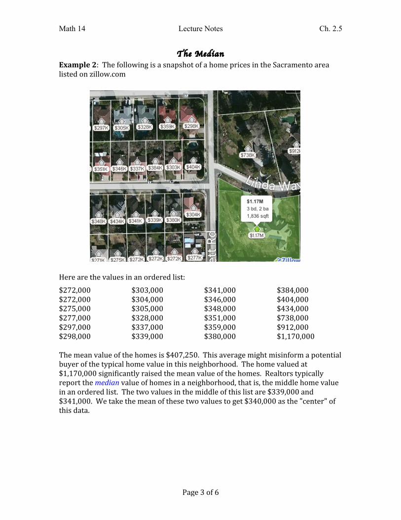
The Median Example 2: The following is a snapshot of a home prices in the Sacramento area listed on zillow.com

Here are the values in an ordered list: $272,000 $272,000 $275,000 $277,000 $297,000 $298,000

$303,000 $304,000 $305,000 $328,000 $337,000 $339,000

$341,000 $346,000 $348,000 $351,000 $359,000 $380,000

$384,000 $404,000 $434,000 $738,000 $912,000 $1,170,000

The mean value of the homes is $407,250. This average might misinform a potential buyer of the typical home value in this neighborhood. The home valued at $1,170,000 significantly raised the mean value of the homes. Realtors typically report the median value of homes in a neighborhood, that is, the middle home value in an ordered list. The two values in the middle of this list are $339,000 and $341,000. We take the mean of these two values to get $340,000 as the "center" of this data.


of 6

The Mode Example 3: At the Tehama campus, the majors/career interests named by students in this class were as follows

Business Administration Business Administration Business Administration Computer Science Computer Science Liberal Studies

Medicine Medicine Medicine Nursing Nursing Nursing

Physician Assistant Psychology Psychology Psychology Psychology Psychology Psychology

From categorical data (non-‐numerical), we can determine a different measure of central tendency, the mode, the most frequently occurring majors in a data set. Which is the most frequently occurring major or career interest?

The Midrange Example 4: Recall from section 2.2 the following data set of test scores on a statistics exam worth 85 points:

72, 76, 53, 68, 72, 85, 46, 77, 36, 81, 49, 73, 68, 65, 70, 71 The instructor of this class may calculate the midrange, which is the mean of the largest and smallest scores, and use that number as a minimum qualifying score for

an intern position. That would be 85+362

=1212= 60.5 .


of 6

Clearly, the $1.17 million home value is an outlier (an extreme data value) and skews the data to the right. In a much larger data set of home values we would see a similar shape, that is, a cluster at the left with a more solid tail sweeping low and to the right of the cluster. For data given only in a frequency distribution, we can find the mean by multiplying the frequency by the midpoint of each class, adding the products together, and dividing the sum by how many data values there are. So for the frequency distribution above the mean is 294, 000 • 9 + 338, 000 • 8 + 383, 000 • 3 + 428, 000 + 744, 000 + 923, 000 + 1,148, 000

24= 405,917.

This is slightly different from the actual mean, but it is clear that the approximation is close.

mean = $407,250

median = $340,000

modal class = $293,000

Note that in a grouped frequency distribution, the modal class of the data set is the midpoint of the most frequently occurring class.

271.5

315.5

360.5

405.5

450.5

495.5

540.5

585.5

630.5

675.5

720.5

765.5

810.5

855.5

900.5

945.5

990.5

1035.5

1080.5

1125.5

1170.5

Home value in thousands (Class limits)

Home value in thousands

(Class boundaries)

Frequency

272 – 315 271.5 – 315.5 9 316 – 360 315.5 – 360.5 8 361 – 405 360.5 – 405.5 3 406 – 450 405.5 – 450.5 1 451 – 495 450.5 – 495.5 0 496 – 540 495.5 – 540.5 0 541 – 585 540.5 – 585.5 0 586 – 630 585.5 – 630.5 0 631 – 675 630.5 – 675.5 0 676 – 720 675.5 – 720.5 0 721 – 765 720.5 – 765.5 1 766 – 810 765.5 – 810.5 0 811 – 855 810.5 – 855.5 0 856 – 900 855.5 – 900.5 0 901 – 945 900.5 – 945.5 1 946 – 990 945.5 – 990.5 0 991 – 1035 990.5 – 1035.5 0 1036 – 1080 1035.5 – 1080.5 0 1081 – 1125 1080.5 – 1125.5 0 1126 – 1170 1125.5 – 1170.5 1

Let's look again at the data set of home values, this time as a frequency distribution and as a histogram with 20 classes. Class width =


of 6

The Weighted Mean Example 5: Suppose an instructor weights scores as follows:

Exams – 80% Quizzes – 10% Homework – 10%

And suppose a student received:

Exam average: 0.81 Quiz average: 0.78 Homework average: 0.85

To calculate this student’s grade, multiply each average by its respective weight and add the results: 0.81 • 0.8 + 0.78 • 0.1 + 0.85 • 0.1 = 0.811 ≈ 81%

Math 14 Lecture Notes Ch. 2 - dgriffinresources.netdgriffinresources.net/m14_02_5.pdf · Math 14...

Documents

Transcript of Math 14 Lecture Notes Ch. 2 - dgriffinresources.netdgriffinresources.net/m14_02_5.pdf · Math 14...