Math 116 { Section 031 Course Notesyiwchen/m116/Notes/note.pdf · · 2016-12-10... (x i) x lim...

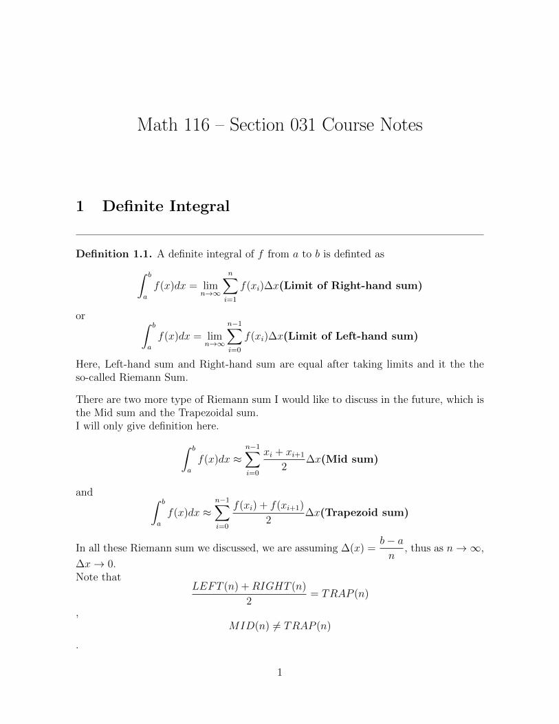
Math 116 – Section 031 Course Notes

1 Definite Integral

Definition 1.1. A definite integral of f from a to b is definted as∫ b

a

f(x)dx = limn→∞

n∑i=1

f(xi)∆x(Limit of Right-hand sum)

or ∫ b

a

f(x)dx = limn→∞

n−1∑i=0

f(xi)∆x(Limit of Left-hand sum)

Here, Left-hand sum and Right-hand sum are equal after taking limits and it the theso-called Riemann Sum.

There are two more type of Riemann sum I would like to discuss in the future, which isthe Mid sum and the Trapezoidal sum.I will only give definition here.∫ b

a

f(x)dx ≈n−1∑i=0

xi + xi+1

2∆x(Mid sum)

and ∫ b

a

f(x)dx ≈n−1∑i=0

f(xi) + f(xi+1)

2∆x(Trapezoid sum)

In all these Riemann sum we discussed, we are assuming ∆(x) =b− an

, thus as n→∞,

∆x→ 0.Note that

LEFT (n) +RIGHT (n)

2= TRAP (n)

,MID(n) 6= TRAP (n)

.

1

Math 116 – Section 031

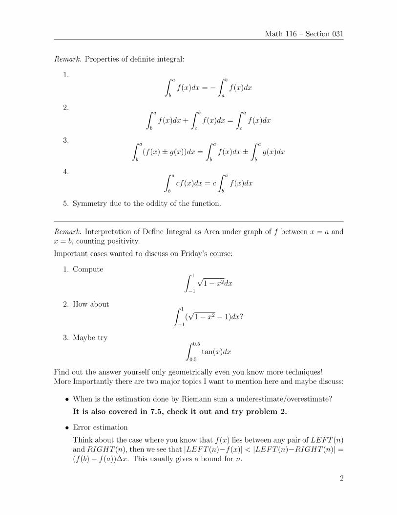
Remark. Properties of definite integral:

1. ∫ a

b

f(x)dx = −∫ b

a

f(x)dx

2. ∫ a

b

f(x)dx+

∫ b

c

f(x)dx =

∫ a

c

f(x)dx

3. ∫ a

b

(f(x)± g(x))dx =

∫ a

b

f(x)dx±∫ a

b

g(x)dx

4. ∫ a

b

cf(x)dx = c

∫ a

b

f(x)dx

5. Symmetry due to the oddity of the function.

Remark. Interpretation of Define Integral as Area under graph of f between x = a andx = b, counting positivity.

Important cases wanted to discuss on Friday’s course:

1. Compute ∫ 1

−1

√1− x2dx

2. How about ∫ 1

−1(√

1− x2 − 1)dx?

3. Maybe try ∫ 0.5

0.5

tan(x)dx

Find out the answer yourself only geometrically even you know more techniques!More Importantly there are two major topics I want to mention here and maybe discuss:

• When is the estimation done by Riemann sum a underestimate/overestimate?

It is also covered in 7.5, check it out and try problem 2.

• Error estimation

Think about the case where you know that f(x) lies between any pair of LEFT (n)and RIGHT (n), then we see that |LEFT (n)−f(x)| < |LEFT (n)−RIGHT (n)| =(f(b)− f(a))∆x. This usually gives a bound for n.

2


Theorem 1.1. The Fundamental Theorem of Calculus is basically the theoremdefined below.If f is continuous on interval [a, b] and f(t) = F ′(t), then∫ b

a

f(t)dt = F (b)− F (a).

Application of the Fundamental Theorem of Calculus

1. Average value of function f(x) in [a, b] is

1

b− a

∫ b

a

f(x)dx

.

Here, think about the integration is analogue to summation in the discrete world,then this average value is the analogue of

xaverage =x1 + x2 + . . .+ xn

1 + 1 + 1 + . . .=x1 + x2 + . . .+ xn

n.

where in the integration case is actually

xaverage =limn→∞

∑n−1i=0 f(xi)∆x

limn→∞∑n−1

i=0 1×∆x=

∫ baf(x)dx∫ ba

1dx=

1

b− a

∫ b

a

f(x)dx

Now, try to work on the rest of problems in the exercise and email me if you have anyquestion, if you think the problems are too hard, I can give you some basic problems towork on first.Problem 5 is going to be discussed in Monday so we have more time.

2 Chapter 6 Anti-derivatives

Anti-derivative of usual functions

1. Try to find the antiderivatives by the graphs

2. Compute an antiderivative using definite integrals.

Suggested Problems: § 6.1 3,7,9,13, 17,29,31,33

Construct antiderivative analytically

3


Definition 2.1. We define the general antiderivative family as indefinite integral.

Remark. ∫Cdx = 0∫

kdx = kx+ C∫xndx =

xn+1

n+ 1+ C, (n 6= −1)∫

1

xdx = ln |x|+ C∫exdx = ex + C∫

cosxdx = sinx+ C∫sinxdx = − cosx+ C

Properties of antiderivatives:

1. ∫(f(x)± g(x))dx =

∫f(x)dx±

∫g(x)dx

2. ∫cf(x)dx = c

∫f(x)dx

Suggested Problems: § 6.2 51-59, 65,71,75

Second FTC (Construction theorem for Antiderivatives)

Theorem 2.1. If f is a continuous function on an interval, and if a is any number inthat interval then the function F defined on the interval as follows is an antiderivativeof f :

F (x) =

∫ x

a

f(t)dt

Suggested Problems: § 6.4 5,7,9,11,17,27,31-34

4


3 Integration Techniques

In this section, we will focus more on how to find the family of antiderivatives that isdetermined by the function we provided, since if we know such family, then given aninitial value of F (x), we can recover the specific antiderivative that we need.

3.1 Guess and Check method

Frankly speaking, this is gambling based on experience.Although it is one of the fundamental method we use to solve problems, for example,it appears in also cryptography with the name Bruce force attack, and it also appearsin computer science with the name Brute force search. However, as you probably know,this is usually not the most systematic or the most efficient way to the solution, and itusually requires either experience on the work or machine that do not rest.

3.2 Integration using Substitution

Exercise as motivation: §6.4 35,37.Similarly, the chain rule of derivative is also extremely useful in finding integral.Theoretically, integration using substitution is using the philosophy that given an inte-gration as

∫f(g(x))g′(x)dx, we will have F (g(x)) + C as its derivative, which is due to

ddx

(F (g(x))) = f(g(x))g′(x), and doing integration on both side will give us the ”substi-tution rule” we want.Technically, you want to recognize the ”g(x)” part in your function, then substitude g(x)as w, with the rule dw = w′(x)dx = dw

dxdx (naively, we do have dw

dxdx = dw! However,

this does not make much sense here which if you are particular interesting, you can askme in person.)Now let us consider an example, to see how is it actually applies. Personally, my favoritealmost trivial example is∫ ∞

0

e−xdx = −∫ −∞0

ew − dw =

∫ 0

−∞ewdw = 1. (Here I let w = −x)

I will explain why is this one interesting in the next subsection, but here there is awarning you may see, Check the up and low bound for your integration! Let ussee another example to see this clearer.∫ π/4

0

tan3 θ

cos2 θdθ =

∫ 1

0

w3dw =1

4, ( Here I take w = cos θ.)

Fast question: Can I do the following integrals? Why?

(1)

∫ π/2

0

tan3 θ

cos2 θdθ or (2)

∫ π/4

−π/4

tan3 θ

cos2 θdθ

Suggested Problems: §7.1 some ex, 81,89,90-96,97,99,109,111,114,125,141,145,147

5


3.3 Integration using partial fractions

Small break after the introduction to substitution, we have this partial fractions.Using the method of the substitution, we can already compute many weird integrationlike

∫2

x−10dx.

Now, how about∫

1x2−1dx? We are out of knowledge about how to do it right now, but

there is an important method we ususally can apply, which is the partial fractions.The idea here is to break 1

x2−1 as a sum:

1

x2 − 1=

1

2(x− 1)+ (− 1

2(x+ 1))

But then now we can compute the integration in the question, since we can definitelycompute

∫1

2(x−1)dx and∫

12(x+1)

dx.In general, we can do this partial fraction to

p(x)

(x− c1)(x− c2) . . . (x− cn)=

A1

x1 − c1+

A2

x2 − c2+ . . .+

Anxn − cn

3.4 Integration by parts

If we call the integration using substitution the masterpiece established on the ChainRule, then I have to say integration by parts is the same thing established on productrule.Similar to the substitution, we reverse our thoughts here.What is exactly happen in the integration by parts is that we are just undoing theproduct rules. Therefore, the key part is recognize your product rule carefully,Consider the product rule:

(uv)′ = u′v + uv′ = u′v + uv′

By some twisted, we will have the following formula for uv′ which we have not seen theadvantages yet.

uv′ = (uv)′u′v

But now, integrate both sides will give us:∫udv =

∫(uv)

∫vdu = uv −

∫vdu

, now if you remember what we talked about in the substitution chapter, you willimmediately recognize that this is what we want.Traditional Example: ∫

ln(x)dx∫cos2 x

Suggested Problems: § 7.2 49,53,55,65,69,73

6


4 Integration Approximation

Estimate the integral is based on the fact that after taking limits of Left/Right/Mid/TrapezoidalRiemann Sum, they are gonna equals and will give the actual integration value, thus ifwe just compute the Riemann sums in finite many block, we will have a value that ispretty much close to the actual integration, and we can refine our calculation by takingmore blocks.Reminder: we have then four ways of estimating an integral using a Riemann Sum:

1. LEFT(n)

2. RIGHT(n)

3. MID(n)

4. TRAP(n)

Think about what they are? Think about Pictures!Is your estimation over/under?

Again, Pictures!(It probably will never make sense without picture.)

1. If the graph of f is increasing on [a, b], then

LEFT (n) ≤∫ b

a

f(x)dx ≤ RIGHT (n)

2. If the graph of f is decreasing on [a, b], then

RIGHT (n) ≤∫ b

a

f(x)dx ≤ LEFT (n)

3. If the graph of f is concave up on [a, b], then

MID(n) ≤∫ b

a

f(x)dx ≤ TRAP (n)

4. If the graph of f is concave down on [a, b], then

TRAP (n) ≤∫ b

a

f(x)dx ≤MID(n)

Suggested Problems: §7.5 1,3,5,16,17,25

7


5 Find Area/Volumes by slicing

• Compute the area of triangle;

• Compute the area of (semi)circle;

• Compute the volume of a sphere;

• Compute the volume of a cone with base radius 5 and height 5;

• Volume of revolution: y = e−x from 0 to 1 around x-axis.

Suggested Problems: §8.1 1-4,10,12,14,16,18,19,21,29,31,37

6 Volumes of Solids of Revolution

There are two methods to find such a volume. One way is using the slicing as we justdiscussed above, which is officially called the Disk Method.

6.1 Disk Method

Check above.

6.2 Shell Method

This is not so intuitive that why will we want to consider other method to integratingany function since we already have this disk method. However, consider the followingexample:Determine the volume of the solid obtained by rotating the region bounded by y =(x− 1)(x− 3)2 and the x-axis about the y-axis.Try to graph it and see why it is bad.Thus, the shell method arises naturally as a different approach, as it integrates along anaxis perpendicular to the axis of revolution.

7 Arc length

Arc Length =

∫ b

a

√1 + (f ′(x))2dx

The function we are integrating might not see as intuitive, but when we think about thepicture of ”small increment” as in class, you will see how it is making sense.Suggested Problems: §8.2 25,27,35,47,49,57,63,65

8


8 Relation of Integration and Physics

Think about what integration is doing. Integral is defined as a limit of the Riemannsum, thus what it is doing is exactly the same as what the Riemann sum is doing,furthermore, you can think definite integral as just infinite block Riemann sum.What we had done in the last section is to find Volumes by integrating, which is thefirst time we figure out what this mysterious ”f(x)” in the integration really is, i.e. if itis an area, then f(x)∆x is actually a volume, and we are summing many slices/shells ofvolumes to get the exact amount of volume of the object.Here, the most essential formula we are using is actually V = Ah, where V is the volumeof prism/cylinder, A is the area, and h is the height. In the most settings above, we willsee S as function of h(which is exactly disk method), or sometimes h is a function of A(what we only deal are the good cases, where S is a function of r and h is a function ofr, since dS is not making sense yet).

We will see in this section that all our important example here comes from a productformula, and what we are going to do is merely same things, integrate the factor parts,get the information of the product.

8.1 Mass/Center of Mass

8.1.1 Mass

Here, the basic formula we are doing is:

1. One dimensional: M = δl where M is the total mass, δ is the density, l is line.

2. Two dimensional: M = δA where M is the total mass, δ is the density, A is Area.

3. Three dimensional (real world): M = δV where M is the total mass, δ is thedensity, V is Volume.

It is confusing that when should one use which, but if you think about what the unit ofthe density is, it will make sense of itself. (Actually, if you think area as the density ofVolume, i.e. think of unit of it as m2 = m3/m, then you will see integration is basicallyintegrating the density to get the total, this is actually the essential picture you shouldhave.)

8.1.2 Center of Mass

This is making more sense if you have any idea on vectors, since then it will naturallybe the average of the vectors, with each vector ”values” differently. Otherwise, you canthink of this as average of weighted points, which is the same thing.The finite version we are doing:

x =

∑ni=1mixiM

=

∑ni=1mixi∑ni=1mi

9


Thus the integration version will be

x =

∫xδdx∫δdx

Generalization to three dimension, we have

x =

∫xδAxdx

Mass, y =

∫yδAydy

Mass, z =

∫zδAzdz

Mass

, whereAx(x), Ay(y), Az(z) are the the area of a slice perpendicular to the x (respectively,y, z)-axis at x (respectively, y, z).Here you can really think of δAx(x) as a kind of general density when you really smashthe whole thing to x axis, so to speak.Suggested Problems: §8.4 2,9,14,15,25,27,33

8.2 Work

Key formula we are using:

Work done = Force ·Distance

orW = F · d

Integration version:

W =

∫ b

a

F (x)dx

(Question: why usually not x = x(F )?)

8.3 Pressure


Pressure = Mass density · g ·Depth.

orp = δgh

(where g is the acceleration due to gravity)

8.4 Force


Force = Pressure · Area

Suggested Problems: §8.5 3,9,12,14,17,23

10


9 Parametric Equations and Polar Coordinate

9.1 Parametric Equations

To represent the motion of a particle in the xy-plane we use two equations, x = f(t)and y = g(t), then at the time t the particle is at the location (f(t), g(t). In this case,we call the equations for x and y the parametric equations, with parametrization t.Remember that, in parametric equation, for the same line, the parametrization is notunique, and the different parametrization encodes two information:1. Speed of the particle.2. Direction of the motion.

9.1.1 Special Parametric Equations

• Parametric Equations for a Straight Line

An object moving along a line through the point (x0, y0), with dx/dt = a anddy/dt = b, has parametric equations x = x0 + at, y = y0 + bt. The slope of the lineis m = b/a.

• Parametric Equations for a circle with radius k

An object moving along a circle of radius k counterclockwise has parametric equa-tions x = k cos(t), y = k sin(t).

9.1.2 Slope and concavity of the curve

As we discussed in class, we can think of this as a result due to chain rule if we havethat y = F (x) as well.But to summarize, we have the slope of the parametrized curve to be

dy

dx=dy/dt

dx/dt

and the concavity of the parametrized curve to be

d2y

dx2=

(dy/dx)/dt

dx/dt

9.1.3 Speed and distance

The instantaneous speed of a moving object is defined to be

v =√

(dx/dt)2 + (dy/dt)2 =√

(vx)2 + (vy)2

11


. The quantity vx = dx/dt is the instantaneous velocity in the x-direction; vy = dy/dt isthe instantaneous velocity in the y-direction. And we call that (vx, vy) to be the velocityvector.Moreover, the distance traveled from time a to b is∫ b

a

v(t)dt =

∫ a

b

√(dx/dt)2 + (dy/dt)2dt

9.2 Polar Coordinate

Polar coordinates is the coordinates determined by specifying the distance of the pointto origin and the angle measured counterclockwise from positive x-axis to the line joiningthe line connecting the point and the origin.

9.2.1 Relation between Cartesian and Polar

Cartesian to Polar:

(x, y)→ (r =√x2 + y2, θ) (Here we have that tan θ = y/x)

Polar to Cartesian:(r, θ)→ (x = r cos θ, y = r sin θ)

9.2.2 Slope, Arc length and Area in Polar Coordinates

By the relation x = r cos θ, y = r sin θ, given a curve r = f(θ), we have that x =f(θ) cos θ, y = f(θ) sin θ, and thus are parametrized equations of parameter θ. Thereforewe have that the slope of to be

dy

dx=dy/dθ

dx/dθ

The arc length from angle a to b is∫ a

b

√(dx/dθ)2 + (dy/dθ)2dθ

Moreover, due to the fact that the area of the sector is 1/2r2θ, we have that for a curver = f(θ), with f(θ) ≥ 0, the area of the region enclosed is

1

2

∫ b

a

f(θ)2dθ

12


10 Differential Equation

Differential equation is the equations that is in the form

dy

dx= f(x, y)

.Note that the solution of the differential equations is usually a family of solution, andis usually not unique.

10.1 Slope Field

To approximate the solution numerically, we need the tool of the slope field. A slopefield is the normal Cartesian coordinates for (x, y) with the little slope defined at thepoint (x, y) drawn at the point. Then we can approximately see the solutions from theslope field already!Moreover,

• Slope field includes the information of (x,y,dy/dx) at a point.

• Follow the slope field, we can recover the graph approximately.

• In the slope field, we can clearly see that there are several equilibrium lines, theycan be categorized as stable/unstable, see definition in 11.5.

10.2 Euler’s method.

• Approximately, we can approximate the original curve’s data using dy/dx at thatpoint.

• More specifically,

y(x1) ≈ y(x0) +dy

dx|x0(x1 − x0)

• Looking at the grid defined by the lines where dydx

= 0, we can tells how thedifferential equation looks like.

• Beware, function of two variables might appears, be sure about its meaning.

• Euler’s Method leads to an underestimate when the curve is concave up, just as itwill lead to an overestimate when the curve is concave down.

10.3 Separation of variables

Given dy/dx = g(x)f(y), we then will have that 1/f(y)dy/dx = g(x), and thus∫1/f(y)dy =

∫g(x)dx

, then we can solve y = h(x) which as the solution from here.

13


10.3.1 General solution to dy/dx = ky

Note that here we have a special case, the general solution to dy/dx = ky is y = Bekx

for any constant B.

10.4 Equilibrium

An equilibrium solution is constant for all values of the independent variable. Thegraph is a horizontal line.An equilibrium is stable if a small change in the initial conditions gives a solution whichtends toward the equilibrium as the independent variable tends to positive infinity.An equilibrium is unstable if a small change in the initial conditions gives a solutioncurve which veers away from the equilibrium as the independent variable tends to positiveinfinity.

Example 10.1. y(t) = Cet has a stable equilibrium y(t) = 0.

Example 10.2. y(t) = Ce−t has a stable equilibrium y(t) = 0.

10.5 How to write down a differential equation?

Follow the steps:

• Begin from the rate, i.e. dy/dx.

• Find out what is each single part that contributes to the rate at a moment, withsign.Here a usual strategy will be to split the rate as two parts: how much is in andhow much is out.

• Now write down formally.

14


11 L’Hopital’s rule

LHopitals rule: If f and g are differentiable and (below a can be ±∞)i)f(a) = g(a) = 0 for finite a,Or ii)limx→a f(x) = limx→a g(x) = ±∞,Or iii)limx→∞ f(x) = limx→∞ g(x) = 0 then

limx→a

f(x)

g(x)= lim

x→a

f ′(x)

g′(x)

11.1 Dominance

We say that g dominates f as x→∞ if limx→∞ f(x)/g(x) = 0.

11.2 How to determine some bad limit?

There are several types of the limits that is ”bad” which requires L’Hopital’s rule tocalculate: 0/0,∞/∞,∞· 0,∞−∞, 1∞, 00,∞0. Although the first two cases we can useL’Hopital’s rule to calculate, the others we cannot use it directly.Read the book, and there are several things that we can consider.

• Consider adding the fractions.

• Consider taking log.

• Consider 1/f(x) so that we can transform ∞ to ’1/0’ or 0 to ’1/∞’.

12 Improper integral

Formal definition of the improper integral I will let you read the book carefully, they arein the box. However, informally, there are two types of improper integral which we justinterpret them as a limit.

• The first case is where we have the limit of the integration goes to infinity, i.e.limb→∞

∫ baf(x)dx.

• The integrand goes to infinity as x→ a.

12.1 Converges or diverges?

The basic question that one want to know about the improper integral is basically is itwell defined?This turns to ask if an improper integral converges or not.There are four ways people ususally use to check this fact.

1. Check by definition, this means check the limit directly.

15


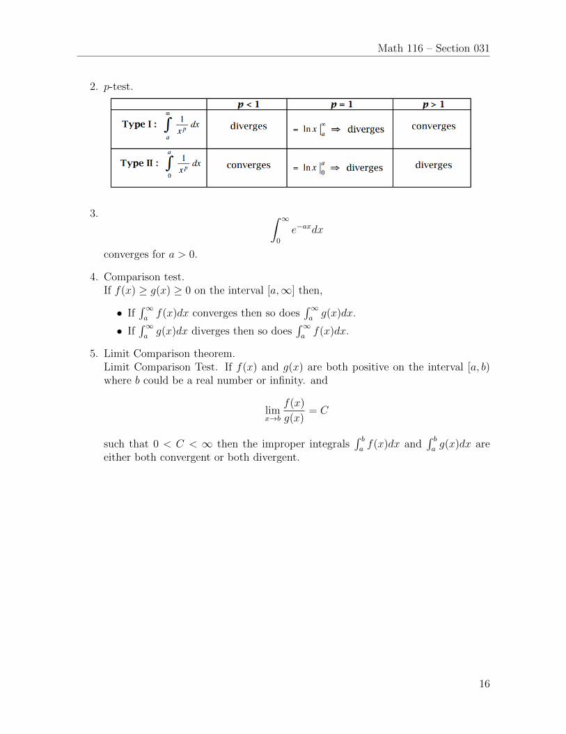
2. p-test.

3. ∫ ∞0

e−axdx

converges for a > 0.

4. Comparison test.If f(x) ≥ g(x) ≥ 0 on the interval [a,∞] then,

• If∫∞af(x)dx converges then so does

∫∞ag(x)dx.

• If∫∞ag(x)dx diverges then so does

∫∞af(x)dx.

5. Limit Comparison theorem.Limit Comparison Test. If f(x) and g(x) are both positive on the interval [a, b)where b could be a real number or infinity. and

limx→b

f(x)

g(x)= C

such that 0 < C < ∞ then the improper integrals∫ baf(x)dx and

∫ bag(x)dx are

either both convergent or both divergent.

16


13 Sequences and Series

13.1 Sequence

Definition 13.1. A sequence is an enumerated collection of objects in which repetitionsare allowed. We denote the sequence a1, a2, . . . , an . . . as (an).

Note that for sequence, there are two things that we will usually concern. The first oneis the convergence of the sequence itself, which is defined as

Definition 13.2. The sequence s1, s2, s3, . . . , sn, . . . has a limit L, written limn→∞ sn =L, if sn is as close to L as we please whenever n is sufficiently large. If a limit, L, exists,we say the sequence converges to its limit L. If no limit exists, we say the sequencediverges.

If we think about the situation more clearly, we will see that, in the definition it actuallyencodes an information: A convergent sequence is bounded. Is the converse true here?Unfortunately, it is not true that a bounded sequence is convergent. However, by thefollowing theorem, we knows when will the bounded sequence becomes convergent.

Theorem 13.1. If a sequence sn is bounded and monotone, it converges.

13.2 Series

There is another thing that we will usually concern.Consider the partial sum of sequence sn, i.e., Sn =

∑ni=1 si, then we will see that the

partial sum forms a sequence as well. Therefore there is a natural question to ask here,when will the sequence Sn of partial sums converges?

Definition 13.3. The associated series for a sequence (an) is defined as the orderedsum

∑∞n=1 an.

Definition 13.4. If the sequence Sn of partial sums converges to S, so limn→∞ Sn = S,then we say the series

∑∞n=1 an converges and that its sum is S. We write

∑∞n=1 an = S.

If limn→∞ Sn does not exist, we say that the series diverges.

There are several properties for convergent series, which is super useful, summarized asbelow.

Theorem 13.2. Convergence Properties of Series

1. If∑∞

n=1 an and∑∞

n=1 bn converge and if k is a constant, then∑∞n=1(an + bn) converges to

∑∞n=1 an +

∑∞n=1 bn.∑∞

n=1 kan converges to k∑∞

n=1 an

2. Changing a finite number of terms in a series does not change whether or not itconverges,

17


3. If limn→∞ an 6= 0 or limn→∞ an does not exist, then∑∞

n=1 an diverges. (Rememberthis!)

4. If∑∞

n=1 an diverges, then∑∞

n=1 an diverges if k 6= 0.

Moreover, there are several test to determine if a series is convergent, detailed discussionabout those is in class.

1. The Integral TestSuppose an = f(n), where f(x) is decreasing and positive.a. If

∫∞1f(x)dx converges, then

∑∞n=1 an an converges.

b. If∫∞1f(x)dx diverges, then

∑∞n=1 an an diverges.

2. p-testThe p-series

∑∞n=1 1/np converges if p > 1 and diverges if p ≤ 1.

3. Comparison TestSuppose 0 ≤ an ≤ bn for all n beyond a certain value.a. If

∑bn converges, then

∑an converges.

b. If∑an diverges, then

∑bn diverges.

4. Limit Comparison TestSuppose an > 0 and bn > 0 for all n. If limn→∞ an/bn = c where c > 0, then thetwo series

∑an and

∑bn either both converge or both diverge.

5. Convergence of Absolute Values Implies ConvergenceIf∑|an| converges, then so does

∑an.

6. The Ratio Test For a series∑an, suppose the sequence of ratios |an+1|/|an| has

a limit: limn→∞ |an+1|/|an| = L, then

• If L < 1, then∑an converges.

• If L > 1, or if L is infinite, then∑an diverges.

• If L = 1, the test does not tell us anything about the convergence of∑an

(Important!).

7. Alternating Series Test A series of the form∑∞

n=1(−1)n−1an = a1 − a2 + a3 −a4 + . . .+ (−1)n−1an + . . . converges if 0 < an+1 < an for all n and limn→∞an = 0.

Moreover, let S = limn→∞ Sn, then we will have |S − Sn| < an+1.

Notably, We say that the series∑an is

• absolutely convergent if∑an and

∑|an| both converge.

• conditionally convergent if∑an converges but

∑|an| diverges.

Test we consider for proving convergence:

18


1. The integral test

2. p-test

3. Comparison test

4. Limit comparison test

5. Check the absolute convergence of the series

6. Ratio Test

7. Alternating Series Test

Test we consider for proving divergence:

1. The integral test

2. p-test

3. Comparison test

4. Limit comparison test

5. Ratio Test

6. Check limn→∞ 6= 0 or limn→∞ does not exist.

13.3 Geometric Series

There is a special series that we learn about, which is the Geometric Series, notice thatthe formula on the right hand side is what we called closed form. A finite geometricseries has the form

a+ ax+ ax2 + · · ·+ axn2 + axn1 =a(1− xn)

1− xFor x 6= 1

An infinite geometric series has the form

a+ ax+ ax2 + · · ·+ axn2 + axn1 + axn + · · · = a

1− xFor |x| < 1

19


14 Power Series and Taylor Series

14.1 Power Series

Definition 14.1. A power series about x = a is a sum of constants times powers of(x− a): C0 + C1(x− a) + C2(x− a)2 + . . .+ Cn(x− a)n + . . . =

∑∞n=0Cn(x− a)n.

If we fix a specific value of x, we can just consider plugging x with the value we have,and convergence here makes sense.

Definition 14.2. For a fixed value of x, if this sequence of partial sums converges to alimit L, that is, if limn→∞ Sn(x) = L, then we say that the power series converges to Lfor this value of x.

Based on the discussion we will see that, The interval of convergence for a power seriesis usually centered at a point x = a, and extends the same length to both side, thus wedenote this length as radius of convergence.

Moreover, each power series falls into one of the three following cases, characterized byits radius of convergence, R.

• The series converges only for x = a; the radius of convergence is defined to beR = 0.

• The series converges for all values of x; the radius of convergence is defined to beR =∞.

• There is a positive number R, called the radius of convergence, such that the seriesconverges for |x− a| < R and diverges for |x− a| > R.

The interval of convergence is the interval between a − R and a + R, including anyendpoint where the series converges.

Then there is a question arises, how to find this radius of convergence then?

This question can be determined by considering using ratio test on the series, assumingx 6= a. The details are included in Chapter 9.5 in the book.

14.2 Taylor Polynomial and Taylor Series

14.2.1 Taylor Polynomial

If we try to approximate the function locally using a polynomial, there is one thing wewant to acquire, i.e. we want the polynomial P (x) with the property that P (n)(a) =f (n)(a) if we approximate the function at the point x = a. Considering merely thesituation about x = 0, recall what we did in the class, we will have the following.

20


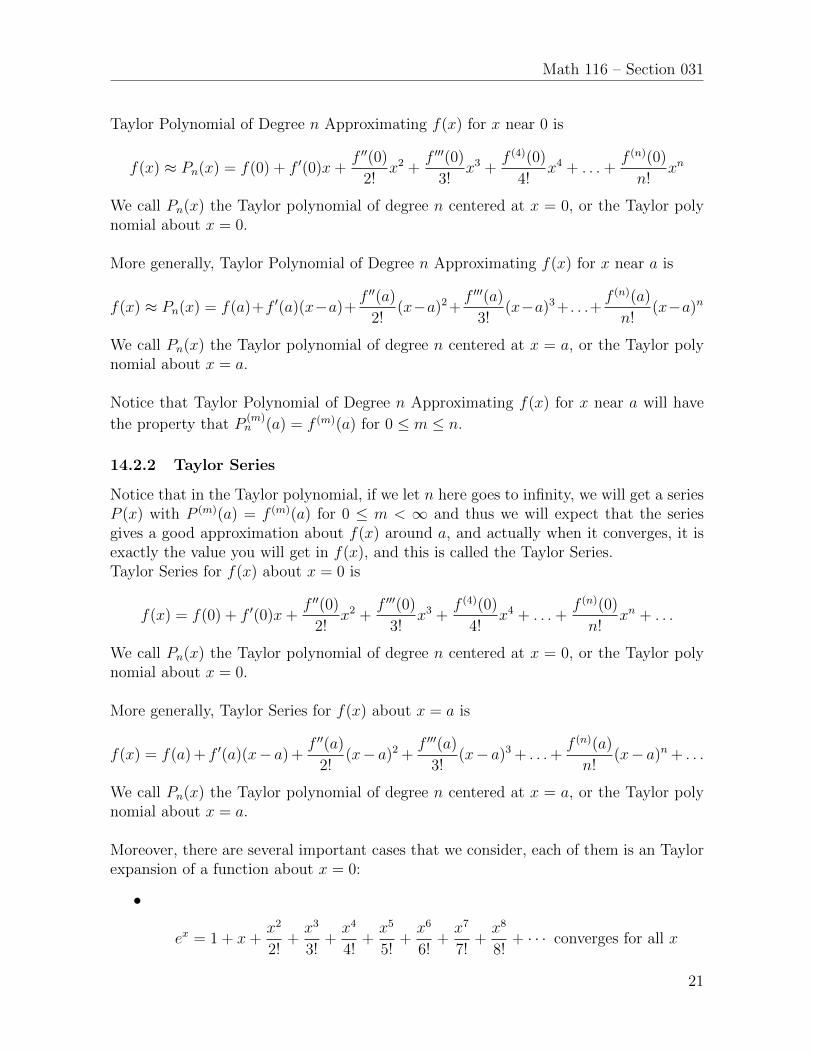
Taylor Polynomial of Degree n Approximating f(x) for x near 0 is

f(x) ≈ Pn(x) = f(0) + f ′(0)x+f ′′(0)

2!x2 +

f ′′′(0)

3!x3 +

f (4)(0)

4!x4 + . . .+

f (n)(0)

n!xn

We call Pn(x) the Taylor polynomial of degree n centered at x = 0, or the Taylor polynomial about x = 0.

More generally, Taylor Polynomial of Degree n Approximating f(x) for x near a is

f(x) ≈ Pn(x) = f(a)+f ′(a)(x−a)+f ′′(a)

2!(x−a)2+

f ′′′(a)

3!(x−a)3+ . . .+

f (n)(a)

n!(x−a)n

We call Pn(x) the Taylor polynomial of degree n centered at x = a, or the Taylor polynomial about x = a.

Notice that Taylor Polynomial of Degree n Approximating f(x) for x near a will have

the property that P(m)n (a) = f (m)(a) for 0 ≤ m ≤ n.

14.2.2 Taylor Series

Notice that in the Taylor polynomial, if we let n here goes to infinity, we will get a seriesP (x) with P (m)(a) = f (m)(a) for 0 ≤ m < ∞ and thus we will expect that the seriesgives a good approximation about f(x) around a, and actually when it converges, it isexactly the value you will get in f(x), and this is called the Taylor Series.Taylor Series for f(x) about x = 0 is

f(x) = f(0) + f ′(0)x+f ′′(0)

2!x2 +

f ′′′(0)

3!x3 +

f (4)(0)

4!x4 + . . .+

f (n)(0)

n!xn + . . .

We call Pn(x) the Taylor polynomial of degree n centered at x = 0, or the Taylor polynomial about x = 0.

More generally, Taylor Series for f(x) about x = a is

f(x) = f(a) + f ′(a)(x− a) +f ′′(a)

2!(x− a)2 +

f ′′′(a)

3!(x− a)3 + . . .+

f (n)(a)

n!(x− a)n + . . .

We call Pn(x) the Taylor polynomial of degree n centered at x = a, or the Taylor polynomial about x = a.

Moreover, there are several important cases that we consider, each of them is an Taylorexpansion of a function about x = 0:

•

ex = 1 + x+x2

2!+x3

3!+x4

4!+x5

5!+x6

6!+x7

7!+x8

8!+ · · · converges for all x

21


•

sin(x) =∞∑n=0

x2n+1

(2n+ 1)!· (−1)n = x− x3

3!+x5

5!− x7

7!+ . . . converges for all x

•

cos(x) =∞∑n=0

x2n

(2n)!· (−1)n = 1− x2

2!+x4

4!− x6

6!+ . . . converges for all x

•

(1 + x)p =∞∑k=0

(p

k

)xk =

∞∑k=0

p!

k!(p− k)!xk =

1 + px+p(p− 1)

2!x2 +

p(p− 1)(p− 2)

3!x3 + · · · converges for − 1 < x < 1.

•

ln(1 + x) =∞∑n=0

(−1)nxn+1

n+ 1= x− x2

2+x3

3− x4

4+ · · · ,

Moreover, we can definitely find Taylor Series based on the existing series using fourmethods:

• Substitude

Example: Taylor Series about x = 0 for f(x) = e−x2

• Differentiate

Example: Taylor Series about x = 0 for f(x) = 1(1−x)2

• Integrate

Example: Taylor Series about x = 0 for f(x) = arctan x (Hint: What is ddx

(arctanx)?)

• Multiply

Example: Taylor Series about x = 0 for f(x) = x2 sinxExample: Taylor Series about x = 0 for f(x) = sinx cosxExample: Taylor Series about x = 0 for f(x) = esinx

22

Math 116 { Section 031 Course Notesyiwchen/m116/Notes/note.pdf · · 2016-12-10... (x i) x lim...

Documents

Transcript of Math 116 { Section 031 Course Notesyiwchen/m116/Notes/note.pdf · · 2016-12-10... (x i) x lim...