NBER WORKING PAPER SERIES

MATCHING WITH COUPLES:STABILITY AND INCENTIVES IN LARGE MARKETS

Fuhito KojimaParag A. PathakAlvin E. Roth

Working Paper 16028http://www.nber.org/papers/w16028

NATIONAL BUREAU OF ECONOMIC RESEARCH1050 Massachusetts Avenue

Cambridge, MA 02138May 2010

We thank Rezwan Haque, and especially Dan Barron and Pete Troyan for superb research assistance.We are also grateful to Joel Sobel and participants at the ERID Matching Conference "Roth and Sotomayor:Twenty Years After" at Duke for comments. Elliott Peranson and Greg Keilin provided invaluableassistance in obtaining and answering questions about the data used in this paper on behalf of NationalMatching Services and the Association of Psychology Postdoctoral and Internship Centers. The NationalScience Foundation provided research support. The views expressed herein are those of the authorsand do not necessarily reflect the views of the National Bureau of Economic Research.

NBER working papers are circulated for discussion and comment purposes. They have not been peer-reviewed or been subject to the review by the NBER Board of Directors that accompanies officialNBER publications.

© 2010 by Fuhito Kojima, Parag A. Pathak, and Alvin E. Roth. All rights reserved. Short sectionsof text, not to exceed two paragraphs, may be quoted without explicit permission provided that fullcredit, including © notice, is given to the source.

Matching with Couples: Stability and Incentives in Large MarketsFuhito Kojima, Parag A. Pathak, and Alvin E. RothNBER Working Paper No. 16028May 2010JEL No. D02,J01

ABSTRACT

Accommodating couples has been a longstanding issue in the design of centralized labor market clearinghousesfor doctors and psychologists, because couples view pairs of jobs as complements. A stable matchingmay not exist when couples are present. We find conditions under which a stable matching exists withhigh probability in large markets. We present a mechanism that finds a stable matching with high probability,and which makes truth-telling by all participants an approximate equilibrium. We relate these theoreticalresults to the job market for psychologists, in which stable matchings exist for all years of the data,despite the presence of couples.

Fuhito KojimaStanford Universityfuhitokojima1979@gmail.com

Parag A. PathakAssistant Professor of EconomicsE52-391CMIT Department of EconomicsCambridge, MA 02142and NBERppathak@mit.edu

Alvin E. RothHarvard UniversityDepartment of EconomicsLittauer 308Cambridge, MA 02138-3001and NBERaroth@hbs.edu

1 Introduction

One of the big 20th century transformations of the American labor market involves the increased

labor force participation of married women, and the consequent growth in the number of two-

career households.1 When a couple needs two jobs, they face a hard problem of coordination

with each other and with their prospective employers. The search and matching process for the

spouses can involve very different timing of searches and hiring. The couple may be forced to make

a decision on a job offer for one member of the couple before knowing what complementary jobs

may become available for the other or what better pairs of jobs might become available elsewhere.

An unusually clear view of this problem can be found in the history of the entry-level labor

market for American doctors. Since the early 1900s, new U.S. medical graduates have been first

employed as “residents” at hospitals, where they work under the supervision of more senior,

licensed doctors. This market experienced serious problems having to do with the timing of

offers and acceptances, and this unraveling of the market led to the creation of a centralized

clearinghouse in the 1950s that drew high rates of participation (see Roth (1984, 2003) and Roth

and Xing (1994) for further details). Medical graduates were almost all men throughout this

period, but by the 1970s there were enough women graduating from medical school so that it

was not unheard of for two new medical graduates to be married to each other.2 Many couples

felt that the existing clearinghouse did not serve them well, and starting in the 1970s, significant

numbers of these couples began seeking jobs outside of the clearinghouse.

Roth (1984) argues that this was because the matching algorithm used until then did not allow

couples to appropriately express preferences. That paper shows that, in a market without couples,

the 1950s clearinghouse algorithm is equivalent to the deferred acceptance algorithm of Gale and

Shapley (1962), and that it produces a stable matching – loosely speaking, this is a matching such

that there is no pair of hospital and doctor who want to be matched with each other rather than

accepting the prescribed matching.3 It then observes that the algorithm often fails to find a stable

matching when there are couples, and argues that a main problem of the mechanism is that (prior

to the 1983 match) it did not allow couples to report preferences over pairs of positions, one for

each member of the couple. Roth and Peranson (1999) designed the current algorithm, which

elicits and uses couples’ preferences over pairs of positions, and this design has been adopted by

1See, for instance, Costa and Kahn (2000) for a description of the trends in the labor market choices forcollege-educated couples since World War II.

2In the 1967-68 academic year, 8% of the graduates of U.S. medical schools were women. By1977-78 this fraction had risen to 21%, and by 2008-09 to 49% (Jonas and Etzel (1998), andhttp://www.aamc.org/data/facts/charts1982to2010.pdf).

3Section 3 provides a precise definition of our stability concept. The evidence suggests that the stability of thematch plays an important role in attracting high rates of participation (Roth, 1990, 1991).

2

more than 40 centralized clearinghouses such as the medical market for American doctors, the

National Resident Matching Program (NRMP).4

But the problem is difficult even if couples are allowed to express their preferences over pairs

of positions, because there does not necessarily exist a stable matching in markets with couples

(Roth, 1984). However, some matching clearinghouses seem to regularly entertain high rates of

participation and appear to have produced matchings that are honored by participants. In fact, it

has been reported that there have only been a few occasions in which a stable matching was not

found over the last decade in several dozen annual markets (Peranson, private communication).

Moreover, in the largest of these markets, the NRMP, Roth and Peranson (1999) run a number of

matching algorithms using submitted preferences from 1993, 1994 and 1995 and find no instance

in which any of these algorithms failed to produce a stable matching. Why do these matching

clearinghouses produce stable outcomes even though existing theory suggests that stable matchings

may not exist when couples are present?

This is the puzzle we address, and this paper argues that the answer may have to do with

the size of the market. We consider a sequence of markets indexed by the number of hospitals,

where doctors’ preferences are drawn from some distribution. When the number of couples does

not grow too fast relative to the market size, under some regularity conditions, we demonstrate

that the probability that a stable matching exists converges to one as the market size approaches

infinity. Moreover, we provide an algorithm that finds a stable matching with a probability that

converges to one as the market size approaches infinity.

In practice, preferences are private information, and the matching clearinghouse needs to

elicit the information from participants. This motivates our analysis of the incentive properties

of a particular matching mechanism in markets with couples. More specifically, we first define

a mechanism similar to Roth and Peranson’s algorithm, used in many existing markets. For

a Bayesian game in which doctors and hospitals submit their preferences to this mechanism,

we establish that truth-telling is an approximate Bayes Nash equilibrium in any market with a

sufficiently large number of hospitals.

As our theoretical analysis only provides limit results, we study data on submitted preferences

from the centralized market for clinical psychologists. In the late 1990s, the market evolved from

a decentralized one to one employing a centralized clearinghouse (Roth and Xing, 1997), where a

key design issue was whether it would be possible to accommodate the presence of couples. Keilin

(1998) reports that under the old decentralized system couples had difficulties coordinating their

internship choices. In 1999, clinical psychologists adopted a centralized clearinghouse using an

4See Roth (2007) for a recent list of these clearinghouses as well as a survey of the literature. See also Sonmezand Unver (2009).

3

algorithm based on Roth and Peranson (1999), where couples are allowed to express preferences

over hospital pairs. We explore a variation of the Roth-Peranson procedure to investigate the

existence of a stable matching with respect to the stated preferences of participants from nine

years of data from 1999-2007. Using our algorithm, we are able to find a stable matching in all

nine years.

Related Literature

This paper is related to several lines of work. First, it is part of research in two-sided matching with

couples. Existing studies are mostly negative: Roth (1984) and unpublished work by Sotomayor

show that there does not necessarily exist a stable matching when there are couples, and Ronn

(1990) shows that it may be computationally hard even to determine if a stable matching exists.

Klaus and Klijn (2005) provide a maximal domain of couple preferences that guarantees the

existence of stable matchings. While their preference domain has a natural interpretation, our

paper finds that preferences of almost all couples in our psychology market data violate their

condition.5 The present paper takes a different approach based on large market arguments to

establish new positive results.

The second line of studies related to this paper is the growing literature on large matching

markets. This paper uses large market arguments similar to Kojima and Pathak (2009). That

paper as well as the current one are motivated by the analysis of Roth and Peranson (1999). They

conduct simulations based on the NRMP data and randomly generated data and find suggestive

evidence that a stable matching is likely to exist and stable matching mechanisms are difficult to

manipulate in large markets. One of their findings is that the number of stable matchings becomes

relatively small in large markets, which might suggest that if a stable matching does not exist in

a finite market, then it is unlikely to exist in a large market. Our analysis finds, on the contrary,

that largeness of the market tends to overcome non-existence in the finite market.

Recently, large market arguments are used by increasingly many studies to analyze incentive

and efficiency of matching mechanisms, not only in two-sided matching (Bulow and Levin, 2006;

Immorlica and Mahdian, 2005) but also in the closely related assignment or one-sided matching

model (Abdulkadiroglu et al., 2008; Che and Kojima, 2010; Kojima and Manea, 2009; Manea,

5Preference restrictions are also used to study incentives for manipulation in matching markets. The restrictionunder which incentive compatibility can be established is often very strong, as shown by Alcalde and Barbera (1994),Kesten (2006b), Kojima (2007), and Konishi and Unver (2006b) for various kinds of manipulations. Similarly, inthe context of resource allocation and school choice (Abdulkadiroglu and Sonmez, 2003), necessary and sufficientconditions for desirable properties such as efficiency and incentive compatibility are strict (Ergin, 2002; Kesten,2006a; Haeringer and Klijn, 2009; Ehlers and Erdil, 2009). Another approach is based on incomplete information(Roth and Rothblum, 1999; Ehlers, 2004, 2008; Kesten, 2009; Erdil and Ergin, 2008).

4

2009). However, the use of large market arguments to establish the existence of a stable matching,

as we do here, is not found in these papers, and appears novel in the matching literature.

While the analysis of large markets is relatively new in the matching literature, it has a long

tradition in economics. For example, Roberts and Postlewaite (1976) and Jackson and Manelli

(1997) show that, under some conditions, the Walrasian mechanism is difficult to manipulate in

large exchange economies. Similarly, Gresik and Satterthwaite (1989) and Rustichini et al. (1994)

study incentive properties of a large class of double auction mechanisms.

Finally, a couple preference is a particular form of complementarity, and this paper can be

put in the context of the larger research program on the role of complementarities in resource

allocation. Complementarities have been identified to cause non-existence of desirable solutions in

various contexts of resource allocation. There has been a recent flurry of investigations on comple-

mentarities and existence problems in auction markets (Milgrom, 2004; Gul and Stacchetti, 2000;

Sun and Yang, 2009), general equilibrium with indivisible goods (Bikhchandani and Ostroy, 2002;

Gul and Stacchetti, 1999; Sun and Yang, 2006), and matching markets (Hatfield and Kominers,

2009; Ostrovsky, 2008; Sonmez and Unver, 2010; Pycia, 2010).

The layout of this paper is as follows. The next section describes some features of the market

for clinical psychologists and lays out a series of stylized facts on matching with couples based on

data from this market. Section 3 defines the model and describes a simple theory of matching with

couples in a finite market. Section 4 introduces the large market assumptions. Section 5 states

our main results on existence, while Section 6 describes our incentive result. Section 7 concludes.

2 The Market for Internships in Professional Psychology

2.1 Background

The story of how design has influenced and reacted to the presence of couples in the NRMP has

parallels in the evolution of the market for internships in professional psychology.6 Roth and

Xing (1997) described this market through the early 1990s. From the 1970’s through the late

1990’s, this market operated in a decentralized fashion (with frequent rule changes), based on

a “uniform notification day” system in which offers were given to internship applicants over the

telephone within a specific time frame (e.g., a 4 hour period on the second Monday in February).

All acceptances and rejections of offers occurred during this period. Keilin (2000) described

6To be clear, we will concentrate on the match run by the Association of Psychology Postdoctoral and Intern-ship Centers (APPIC) for predoctoral internships in psychology, which involves clinical, counseling, and schoolpsychologists. (This is distinct from the postdoctoral match in neuropsychology.)

5

the system as “problematic, subject to bottlenecks and gridlock, encouraging the violation of

guidelines, and resulting in less-than-desirable outcomes for participants.”

In 1998-1999, the Association of Psychology Postdoctoral and Internship Centers (APPIC)

switched to a system in which applicants and internship sites were matched by computer. A major

debate in this decision was whether a centralized system could handle the presence of couples. In

the old decentralized scheme it was challenging for couples to coordinate their internship choices.

Keilin (1998) reports that one partner could be put in the position of having to make an immediate

decision about an offer without knowing the status of the other partner. Following the reforms of

the National Resident Matching Program, a new scheme which allowed couples to jointly express

their preferences was adopted.

With the permission of the APPIC, the company which runs the matching process, National

Matching Services, provided us with an anonymized dataset of the stated rank order lists of single

doctors, couples and hospitals and hospital capacities for the first nine years of the centralized

system. Because of privacy concerns, these data do not include any demographic information on

applicants, and includes only limited identifying information on programs.

2.2 Stylized facts

This section identifies some stylized facts from the internship market for professional psychologists.

Other matching markets with couples appear to share many of the features with this market, as

we highlight below.

The data are the stated preferences of market participants, so their interpretation may require

some caution. There are at least two parts to the process by which market participants form

their preferences: (1) they determine which applicants or internship programs may be attractive,

and participate in interviews, and (2) after interviewing, they determine their rank ordering over

the applicants or internship programs they have interviewed. The model in this paper and the

data do not allow us to say much about the first stage of the application process. In determining

where to interview, applicants likely factor in the costs of traveling to interviews, the program’s

reputation and a host of other factors. Programs consider, among other things, the applicant’s

recommendation letters and suitability for their program in deciding whom to interview. Once

market participants have learned about each other, they must come up with their rank ordering.

For the empirical analysis in this section, we abstract away from the initial phase of mutual

decisions of whom to interview, and our interpretation is that the data reflect the preferences

formed after interviews.

Even with this interpretation, the reported post-interview preferences may be manipulations

6

of the true post-interview preferences of market participants since truth-telling is not a domi-

nant strategy for all market participants. However, there are at least two reasons why treating

submitted preferences as true preferences may not be an unrealistic approximation. First, as

noted in Section 6, the organizers of the APPIC match emphasize repeatedly that market partic-

ipants should declare their preferences truthfully. Second, as we will see, Theorem 2 in Section 6

demonstrates that truthtelling is an approximate equilibrium in large markets.

Table 1 presents some summary statistics on the market. On average, per year, there are 3,010

single applicants and 19 pairs of applicants who participate as couples. In early years, there were

just under 3,000 applicants, but the number of applicants has increased slightly in the most recent

years. The number of applicants who participate as couples has remained relatively small, varying

between 28 and 44, which is about 1% of all applicants.7 In the National Resident Matching

Program, from 1992-2009, there were on average 4.4% of applicants participating as couples, with

slightly more couples participating in the most recent years (NRMP, 2009).

Fact 1: Applicants who participate as couples constitute a small fraction of all participating

applicants.

Panel A of Table 1 shows the length of the rank order lists for applicants and programs. On

average across years, single applicants rank between 7 and 8 programs. Since there are 1,094

programs on average, this means that the typical applicants ranks less than 1% of all possible

programs. Even at the extreme, a single applicant ranks at most 6.7% of all possible programs.

In the NRMP, the length of the applicant preference list is about 7-9 programs, which would be

roughly 0.3% of all possible programs.8 This may not be surprising because an applicant typically

ranks a program only after she interviews at the program.

Fact 2: The length of single applicants’ rank order lists is small relative to the number of possible

programs.

Each entry in the rank order list of a couple is a pair of programs (or being unmatched). The

typical rank order list of couples averages 81 program pairs. Since the rank order list of a couple

has entries for both members, there are many duplicate programs, so we also report the number of

distinct programs ranked by a couple. On average, there are 10 distinct programs listed by each

couple member, which is larger than the average number of distinct programs listed by a single

7As the example in the next section shows, even one couple in the market may lead to non-existence of a stablematching.

8This information is not available separately for single applicants and those who participate as couples in theNRMP.

7

applicant. The maximum number of distinct programs ranked by a couple member is 1.9% of all

programs.

Fact 3: Applicants who participate as couples rank more programs than single applicants. How-

ever, the number of distinct programs ranked by a couple member is small relative to the number

of possible programs.

The next issue we examine is the distribution of applicant preferences. In Figure 1, we explore

the popularity of programs in our data. For each program, we compute the total number of

students who rank that program as their top choice. We order programs by this number, with

the program with the highest number of top choices on the left and programs that no one ranks

as their top choice on the right. Figure 1 shows the distribution of popularity for 2003. In this

year, the most popular program was ranked as the top choice by 19 applicants, and there are 189

programs that are not ranked as a top choice by any applicant. The other years of our dataset

display a similar pattern. Averaged across all years, the most popular program is ranked as a top

choice by 24 applicants, and about 208 programs are not ranked as a top choice by anyone. The

fraction of applicants ranking the most popular program as their first choice is only 0.8%. (Recall

that these are preferences stated after interviews have been conducted, so it does not preclude the

possibility that there are popular programs that receive many applications but only interview a

small subset of applicants.)

Fact 4: The most popular programs are ranked as a top choice by a small number of applicants.

The only identifying information we have on programs are geographic regions where they are

located. The eleven geographic regions in our dataset are ten regions in the US, each of which

corresponds to the first digit of the zip code of the program’s location, and one region for all of

Canada. Figure A1 illustrates these regions and shows the number of programs in each region.

The Figure shows that programs are concentrated on the West Coast and in the Northeast. In

Table 1, we report the number of distinct regions ranked by applicants. Half of single applicants

rank at most two regions. Couples, on the other hand, tend to rank slightly more regions.

For a given couple rank order list, we also compute the fraction of entries on their submitted

list that have both jobs in the same region. On average, 73% of a couple’s rank order list is for

programs in the same region.

Fact 5: A pair of internship programs ranked by doctors who participate as a couple tend to be in

the same region.

8

In the psychology market, there are about 1,100 internship programs. The average capacity is

about 2.5 seats, and more than three quarters of programs have three or fewer spots. The total

capacity of internship programs is smaller than the total number of applicants who participate,

which implies that each year there will be unmatched applicants. This is also true in the NRMP

where the number of positions per applicant ranges from 0.75-0.90 over the period 1995-2009

(NRMP, 2009).

Even though there are more applicants than programs, in the APPIC match, there are a sizable

number of programs that are unfilled at the end of the regular match. According to the APPIC’s

statistics, during 1999-2007, on average 17% of programs had unfilled positions, and these were

filled in a decentralized email aftermarket called the “Clearinghouse.” In the NRMP, a similar

proportion of programs had unfilled seats. In 2009, for instance, 12% of programs had unfilled

positions, and these are filled in a an aftermarket called the “Scramble.”

Fact 6: Even though there are more applicants than positions, many programs still have unfilled

positions at the end of the centralized match.

2.3 Stable Matchings in the Market for Psychologists

We next investigate whether a stable matching exists in the psychologist market.9 Roughly speak-

ing, this is a matching such that there is no pair of hospital and applicant who prefer each other

to the prescribed matching.10 We use a variant of the procedure by Roth and Peranson (1999)

to compute a stable matching.11 For each of the 9 years of data, a stable matching exists in

the market with couples. Table 2 shows that, averaged across years, more than a third of single

applicants obtain their top choice averaged across each year in this stable matching, and 18% of

9The model we analyze in this paper allows employers to have preferences over sets of applicants provided thatthe preferences are responsive. Our data on program rank order lists consist only of preferences over individualapplicants. We do not know, for instance, whether a program prefers their first and fourth ranked applicantsover their second and third ranked applicants. To compute a stable matching in the market for psychologists,it is necessary to specify how comparisons between individual applicants relate to comparisons between sets ofapplicants. For the empirical computation, when comparing sets of applicants D1 and D2, we assume that D1 ismore preferred to D2 if the highest individually ranked applicant in D1 who is not in D2 is preferred to the highestindividual ranked applicant in D2 who is not in D1. This would imply that the first and fourth ranked applicantare preferred over the second and third ranked applicant. (We take advantage here of the more flexible formulationof preferences over sets that we employ, compared to that used in practice.)

10Section 3 provides a precise definition of our stability concept.11Our variation has a different sequencing of applications from single applicants and couples than that described

in Roth and Peranson (1999). That paper gives some evidence that these sequencing decisions have little impacton the success of the procedure.

9

couples obtain their top choice.12 The number of unassigned couples is small (only about 5% of

couples) while almost 20% of single applicants are unassigned.

Fact 7: A stable matching exists in all nine years in the market for psychologists.

We also compare the assignment of single applicants at the stable matching we find in a

market with couples to their assignment in the applicant-optimal stable matching in a market

without couples in Table 2. While adding couples to the market could in principle affect the

assignment received by many single applicants, in practice it has little effect. This can be seen

by comparing the overall distribution of choice received for single applicant in a stable matching

in markets without couples and with couples. Moreover, Table 3 reports the exact number of

single applicants who receive a less preferred assignment in the market with couples. On average,

there are 19 couples or 38 applicants who participate as couples in the market and because of

their presence, only 63 single applicants obtain a lower choice. This corresponds to about 3 single

applicants obtaining a different assignment per couple.

Fact 8: Across stable matchings, most single applicants obtain the same position in the market

without couples as in the market with couples.

In summary, this section describes some stylized facts that influence our choice of modeling

assumptions. For the psychologist market, we are able to find a stable matching for each year for

which we have data, which motivates our search for an existence result.

3 A Simple Theory of Matching with Couples

3.1 Model

A matching market consists of hospitals, doctors, and their preferences. Let H be the set of

hospitals plus an outside option ∅ for doctors. S is the set of single doctors and C is the set of

couples of doctors. Each couple is denoted by c = (f,m), where f and m denote the first and

second members of couple c respectively. When we need to refer to the members of a specific

couple c, we sometimes write (fc,mc). Let F = {f |(f,m) ∈ C for some m} and M = {m|(f,m) ∈C for some f} be the sets of first and second members that form couples. Let D = S ∪F ∪M be

the set of doctors.12We focus on a particular stable matching in the market with couples, since we are unable to compute the entire

set of stable matchings. There may be a reason to suspect that this set is small. In Table A.1 in the appendix,we compute stable matchings in the market without couples and find that very few applicants and programs havedifferent assignments across the applicant-optimal and program-optimal stable matchings.

10

Each single doctor s ∈ S has a preference relation Rs over H. We assume that preferences are

strict: if hRsh′ and h′Rsh, then h = h′. We write hPsh

′ if hRsh′ and h 6= h′. If hPs∅, we say that

hospital h is acceptable to single doctor s.

Each couple c ∈ C has a preference relation Rc over H × H, pairs of hospitals (and being

unmatched). We assume that preferences of couples are strict with Pc denoting the asymmetric

part of Rc. If (h, h′)Pc(∅, ∅), then we say that pair (h, h′) is acceptable to couple c. We say that

hospital h is listed by Rc if there exists h′ ∈ H such that either (h, h′)Pc(∅, ∅) or (h′, h)Pc(∅, ∅).Each hospital h ∈ H \{∅} has a preference relation over 2D, all possible subsets of doctors. We

assume preferences of hospitals are strict. Let h ∈ H \ {∅} and κh be a positive integer. We say

that preference relation �h is responsive with capacity κh if it ranks a doctor independently

of her colleagues and disprefers any set of doctors exceeding capacity κh to being unmatched (see

Appendix A.1 for a formal definition). We follow much of the matching literature and assume

that hospital preferences are responsive throughout the paper. Let Rh be the corresponding

preference list of hospital h, which is the preference relation over individual doctors and ∅.We write dPhd

′ if dRhd′ and d 6= d′. We say that doctor d is acceptable to hospital h if dPh∅. We

write �H= (�h)h∈H . We refer to a matching market Γ as a tuple (H,S,C, (�h)h∈H , (Ri)i∈S∪C).

We proceed to define our stability concept in markets with couples. The descriptions are

necessarily somewhat more involved than those in the existing literature because we allow for

capacity of hospitals larger than one (we will elaborate on the issue in Section 3.1.1). First, it is

convenient to introduce the concept of hospital choices over permissible sets of doctors. For any

set of doctors and couples D′ ⊆ D ∪ C, define

A(D′) = {D′′ ⊆ D|∀s ∈ S, if s ∈ D′′ then s ∈ D′,

∀c ∈ C, if {fc,mc} ⊆ D′′, then (fc,mc) ∈ D′,

if fc ∈ D′′ and mc 6∈ D′′, then fc ∈ D′,

if fc 6∈ D′′ and mc ∈ D′′, then mc ∈ D′}.

In words, A(D′) is the collection of sets of doctors available for a hospital to employ when doctors

(or couples of doctors) D′ are applying to it. Underlying this definition is the distinction between

applications by individual couple members and those by couples as a whole. For example, if

(f,m) ∈ D′∩C but f,m /∈ D′, then the couple is happy to be matched to the hospital if and only

if both members are employed together, while if (f,m) /∈ D′ but {f,m} ⊆ D′, then the couple is

happy to have one member matched to the hospital but not together.

For any set D′ ⊆ D ∪C, define the choice of hospital h given D′, Chh(D′), to be the set such

11

that

• Chh(D′) ∈ A(D′),

• Chh(D′) �h D′′ for all D′′ ∈ A(D′).

The choice Chh(D′) is the most preferred subset of doctors among those in D′ such that each

couple is either chosen or not chosen together if they apply as a couple.13

A matching specifies which doctors are matched to which hospitals (if any). Formally, a

matching µ is a function defined on the set H ∪ S ∪ C, such that µ(h) ⊆ D for every hospital h,

µ(s) ∈ H for every single doctor s, and µ(c) ∈ H ×H for every couple c where

• µ(s) = h if and only if s ∈ µ(h) and

• µ(c) = (h, h′) if and only if fc ∈ µ(h) and mc ∈ µ(h′).

When there are only single doctors in D′, the set A(D′) is simply the set of subsets of D′. Hence

the choice Chh(D′) is the subset of D′ that is the most preferred by h. This is the standard

definition of Chh(·) in markets without couples (see Roth and Sotomayor (1990) for example),

and hence the current definition is a generalization of the concept to markets with couples.

A matching is individually rational if no player can be made better off by unilaterally

rejecting some of the existing partners (see Appendix A.1 for a formal definition). We define

different cases of a block as follows:

(1) A pair of a single doctor s and a hospital h is a block of µ if hPsµ(s) and s ∈ Chh(µ(h)∪s).

(2) (a) A coalition (c, h, h′) ∈ C × H × H of a couple and two hospitals, where h 6= h′, is a

block of µ if

• (h, h′)Pcµ(c),

• fc ∈ Chh(µ(h) ∪ fc), and

• mc ∈ Chh′(µ(h′) ∪mc).

(b) A pair (c, h) ∈ C ×H of a couple and a hospital is a block of µ if

• (h, h)Pcµ(c) and

• {fc,mc} ⊆ Chh(µ(h) ∪ c).

A matching µ is stable if it is individually rational and there is no block of µ.

13We denote a singleton set {x} simply by x whenever there is no confusion. This formulation of hospitalpreferences involving couples is more general than currently implemented in practice, where hospitals’ preferencesare elicited only over individual members of a couple.

12

3.1.1 Discussion of the solution concepts

Models of matching with couples where hospitals have multiple positions are a particular form

of many-to-many matching because each couple may seek two positions.14 Various definitions of

stability have been proposed for many-to-many matching, which differ based on the assumptions on

what blocking coalitions are allowed (Sotomayor, 1999, 2004; Konishi and Unver, 2006a; Echenique

and Oviedo, 2006). Consequently, there are multiple possible stability concepts in matching with

couples. The present definition of stability allows us to stay as close to the most commonly used

pairwise stability as possible, by assuming away deviations involving large groups. Ruling out

large coalitions appears to be reasonable because identifying and organizing large groups of agents

may be difficult.

It is nevertheless important to understand whether our analysis is sensitive to a particular

definition of stability. To address this issue, in Appendix A.2 we present an alternative definition

of stability that allows for larger coalitions to block a matching. We show that all the results of

this paper hold under that definition as well.

Most studies in matching with couples have focused on the case in which every hospital has

capacity one.15 Following the standard definition of stability in such models (see Klaus and Klijn

(2005) for instance), we say that a matching µ is unit-capacity stable if

(1) µ is individually rational,

(2) there exists no single doctor-hospital pair s, h such that hPsµ(s) and sPhµ(h), and

(3) there exists no coalition by a couple c = (f,m) ∈ C and hospitals (or being unmatched)

h, h′ ∈ H with h 6= h′ such that (h, h′)Pcµ(c), fRhµ(h) and mRh′µ(h′).16

Our concept of stability is equivalent to the unit-capacity stability as defined above if every

hospital has responsive preferences with capacity one. To see this, first observe that condition

(3) of unit-capacity stability is equivalent to the nonexistence of a block as defined in condition

(2a) of our stability concept. Moreover, condition (2b) of our stability concept is irrelevant when

each hospital has capacity one because a hospital with capacity one never prefers to match with

14More precisely, Hatfield and Kojima (2008, 2009) point out that the model is subsumed by a many-to-manygeneralization of the matching model with contracts as analyzed by Hatfield and Milgrom (2005).

15Some papers consider multiple positions of hospitals but treat a hospital with capacity larger than one asmultiple hospitals with capacity one each. This approach is customary and innocuous when there exists no couplebecause most stability concepts are known to coincide in that setting (Roth, 1985). However the approach hasa consequence if couples exist since it leads to a particular stability concept. A different modeling approach ispursued by McDermid and Manlove (2009).

16We adopt the notational convention that dR∅d′ for any d, d′ ∈ D ∪ ∅.

13

two members of a couple. Finally, the remaining conditions for unit-capacity stability have direct

counterparts in our definition of stability. Thus the stability concept employed in this paper is a

generalization of the standard concept to the case where hospitals have multiple positions.

Also note that our stability concept is equivalent to the standard definition of (pairwise)

stability when there exist no couples. More specifically, condition (2) of our stability concept

is irrelevant if couples are not present, and condition (1) is equivalent to the nonexistence of

a blocking pair which, together with individual rationality, defines stability in markets without

couples.

3.2 The Problem with Couples

We illustrate how the existence of couples poses problems in the theory of two sided matching. To

understand the role of couples, however, it is useful to start by considering a matching without

couples. In that context, the (doctor-proposing) deferred acceptance algorithm defined below

always produces a stable matching (Gale and Shapley, 1962).

Algorithm 1. Doctor-Proposing Deferred Acceptance Algorithm

Input: a matching market (H,S, (�h)h∈H , (Rs)s∈S) without couples.

• Step 1: Each single doctor applies to her first choice hospital. Each hospital rejects its

least-preferred doctor in excess of its capacity and all unacceptable doctors among those who

applied to it, keeping the rest of the doctors temporarily (so doctors not rejected at this step

may be rejected in later steps).

In general,

• Step t: Each doctor who was rejected in Step (t-1) applies to her next highest choice (if

any). Each hospital considers these doctors and doctors who are temporarily held from the

previous step together, and rejects the least-preferred doctors in excess of its capacity and all

unacceptable doctors, keeping the rest of the doctors temporarily (so doctors not rejected at

this step may be rejected in later steps).

The algorithm terminates at a step where no doctor is rejected. The algorithm always ter-

minates in a finite number of steps. At that point, all tentative matchings become final. Gale

and Shapley (1962) show that for any given market without couples, the matching produced by the

deferred acceptance algorithm is stable. Furthermore, they show that it is the doctor-optimal stable

matching, the stable matching that is weakly preferred to any other stable matching by all doctors.

14

By contrast, stable matchings do not necessarily exist when there exists a couple in the market

(shown by Roth (1984) and an unpublished work by Sotomayor). This fact is illustrated in the

following example, based on Klaus and Klijn (2005).

Example 1. Let there be a single doctor s and a couple c = (f,m) as well as two hospitals h1 and

h2, each with capacity one. Suppose the acceptable matches for each agent, in order of preference,

are given by:

Rc : (h1, h2) Rs : h1, h2

�h1 : f, s �h2 : s,m.

We illustrate that there is no stable matching in this market, by considering each possible match-

ing.

(1) Suppose µ(c) = (h1, h2). Then single doctor s is unmatched. Thus single doctor s and

hospital h2 block µ because s prefers h2 to her match µ(s) = ∅ and h2 prefers s to its match

µ(h2) = m.

(2) Suppose µ(c) = (∅, ∅).

(a) If µ(s) = h1, then (c, h1, h2) blocks µ since couple c prefers (h1, h2) to their match

µ(c) = (∅, ∅), hospital h1 prefers f to its match µ(h1) = s and hospital h2 prefers m to

its match µ(h2) = ∅.

(b) If µ(s) = h2 or µ(s) = ∅, then (s, h1) blocks µ since single doctor s prefers his first

choice hospital h1 to both hospital h2 and ∅ while h1 prefers s to its match µ(h1) = ∅.

Klaus and Klijn (2005) identify a sufficient condition to guarantee the existence of a stable

matching called weak responsiveness. A couple’s preferences are said to be responsive if an im-

provement in one couple member’s assignment is an improvement for the couple. Preferences

are said to be weakly responsive if the requirement applies to all acceptable positions.17 The

preferences of couples in Example 1 do not satisfy this condition. If, for instance, the couple’s

preferences are (h1, h2), (h1, ∅), (∅, h2), (∅, ∅), in order of preference, then it satisfies responsive-

ness and a stable matching exists. Klaus and Klijn (2005) write that “responsiveness essentially

excludes complementarities in couples’ preferences.” They showed that:

(1) if the preferences of every couple are weakly responsive, then there exists a stable matching.

17See Klaus et al. (2009) for formal definition.

15

(2) if there is at least one couple whose preferences violate weak responsiveness while satisfying

a condition called “restricted strict unemployment aversion,” then there exists a preference

profile of other agents such that preferences of all other couples are weakly responsive but

there exists no stable matching.

Their second result says that the class of weakly responsive preferences is the “maximal do-

main” of preferences. That is, it is the weakest possible condition that can be imposed on indi-

vidual couples’ preferences that guarantees the existence of stable matchings.18

There seem to be many situations in which couple preferences violate weak responsiveness.

One reason may be geographic, as stated as Fact 5 in Section 2.2: both programs ranked as a pair

by a couple tend to be in the same geographic region. For example, the first choice of a couple of

medical residents may be two residency programs in Boston and the second may be two programs

in Los Angeles, while one member working in Boston and the other working in Los Angeles could

be unacceptable because these two cities are too far away from each other. The coordinator of the

Association of Psychology Postdoctoral and Internship Centers (APPIC) matching program writes

in Keilin (1998) that “most couples want to coordinate their internship placements, particularly

with regard to geographic location.” This suggests that violation of weak responsiveness due to

geographic preferences is one of the representative features of couple preferences.19

To further study this question empirically, we analyze the data on the stated preferences of

couples from the APPIC.20 During years for which we have data (1999–2007), preferences of only

one couple out of 167 satisfy weak responsiveness. Thus the data suggest, in light of the results

of Klaus and Klijn (2005), that it is virtually impossible to guarantee the existence of a stable

matching in such markets with couples based on a domain restriction of preferences.

However, the fact that the preferences of the overwhelming majority (166 out of 167) of couples

violate weak responsiveness does not mean that a stable matching does not exist in the psychologist

market. Stable matchings have been found in many labor markets despite the presence of couples,

and as we described in Section 2.3, we find a stable match for each of the nine years of the

psychology market for which we have data. This motivates our desire to understand what market

features enable the existence of stable matchings most of the time, when the known sufficient

conditions on couples’ preferences do not guarantee existence.

18Hatfield and Kominers (2009) show that the substitutes condition is a maximal domain in the absence ofrestricted strict unemployment aversion.

19For an investigation of couple decision making in the market for new Ph.D. economists, see Helppie andMurray-Close (2010).

20Since truth-telling is not necessarily a dominant strategy for couples, the use of stated preferences is potentiallyproblematic. However, Theorem 2 in this paper provides formal defense for this assumption by demonstrating thattruthtelling is an approximate equilibrium in large markets.

16

3.3 Sequential Couples Algorithm

The original deferred acceptance algorithm does not incorporate applications by couples. We

consider an extension of the algorithm, which we call the sequential couples algorithm. While

we defer a formal definition to Appendix A.3 for expositional simplicity, we offer an informal

description as follows.

(1) run a deferred acceptance algorithm for a sub-market composed of all hospitals and single

doctors, but without couples,

(2) one by one, place couples by allowing each couple to apply to pairs of hospitals in order of

their preferences (possibly displacing some doctors from their tentative matches), and

(3) one by one, place singles who were displaced by couples by allowing each of them to apply

to a hospital in order of her preferences.

We say that the sequential couples algorithm succeeds if there is no instance in the algorithm

in which an application is made to a hospital where an application has previously been made

by a member (or both members) of a couple except for the couple who is currently applying.

Otherwise, we declare a failure and terminate the algorithm.

Failure of the sequential couples algorithm does not mean that a stable matching does not

exist. Therefore, in practice, a matching clearinghouse would be unlikely to declare failure when

the sequential couples algorithm fails, but would instead consider some procedure to try to assign

the remaining couples and find a stable matching. This is the main idea behind the Roth-Peranson

algorithm (Roth and Peranson, 1999), which is the basis for the mechanism used in the NRMP,

APPIC, and other labor markets. If the sequential couples algorithm would succeed, then the

Roth-Peranson algorithm produces the matching reached by the sequential couples algorithm.

However, the sequential couples algorithm and the Roth-Peranson algorithm are different in two

aspects.21

First, where the sequential couples algorithm fails, the Roth-Peranson algorithm proceeds and

tries to find a stable matching. The algorithm identifies blocking pairs, eliminating instances of

instability one by one, in a manner similar to Roth and Vande Vate (1990). Note that since a stable

matching does not necessarily exist in markets with couples, the Roth-Peranson algorithm could

cycle without terminating. However, the algorithm forces termination of a cycle and proceeds

21A complete description of the Roth-Peranson algorithm, specifically how the algorithm terminates cycles andproceeds with processing, is not publicly available, but a more detailed description than the one provided here isoffered by Roth and Peranson (1999).

17

with processing other applicants. This sometimes ultimately results in a stable matching, and

sometimes no stable matching is found. Second, in the Roth-Peranson algorithm, when a couple

is added to the market with single doctors, any single doctor who is displaced by the couple is

placed before another couple is added. By contrast, the sequential couples algorithm holds any

displaced single doctor without letting her apply, until it processes applications by all couples.22

The reason we focus on this simplified procedure is that the success of the sequential couples

algorithm turns out to play an important role as the next proposition relates it to the existence

of a stable matching (the proof is in Appendix A.3).

Lemma 1. If the sequential couples algorithm succeeds, then the resulting matching is stable.

To illustrate the main idea of Lemma 1, we consider how the sequential couples algorithm

proceeds for the market in Example 1. In Step 1 of the algorithm, we run the doctor-proposing

deferred acceptance algorithm in the sub-market without couples. Single doctor s proposes to

hospital h1 and is assigned there. Then in Step 2, we let couple c apply to their top choice

(h1, h2). Couple member f is preferred to s by h1 and couple member m is preferred to a vacant

position by h2. Thus f and m are tentatively assigned to h1 and h2 respectively while s is rejected.

Then in Step 3, we let s apply to her next highest choice. In this case, she applies to hospital h2,

where a couple member m has applied and been assigned before. At this point we terminate the

algorithm and declare that it has failed.

To see why declaring a failure of the sequential couples algorithm is useful, suppose that we

hypothetically continue the algorithm by allowing h2 reject m as h2 prefers s to m. Then the

couple prefers being unassigned rather than having only f be matched to h1, so doctor f would

like to withdraw his assignment from hospital h1. Suppose we terminate the algorithm at this

point once f becomes unmatched. Then the resulting matching assigns no doctor to h1 and s to

h2. This matching is unstable because doctor s can block with hospital h1. On the other hand,

if we continue the algorithm further by allowing s to match with h1, then the resulting matching

is identical to the one obtained at the end of Step 1 of the sequential couples algorithm. This

suggests that reasonable algorithms would cycle without terminating in this market.

The idea of declaring failure of the sequential couples algorithm is to avoid a situation like the

above example, and turns out to be a useful criterion for judging whether the algorithm produces

a stable matching. Of course, the algorithm sometimes fails even if there exists a stable matching,

so the success of the algorithm is only a sufficient condition for the existence of a stable matching.

What is remarkable is that looking at this particular sufficient condition turns out to be enough

22As we will point out subsequently, our result also holds if we follow the sequencing of the Roth-Peransonalgorithm. We chose the current definition of the sequential couples algorithm for expositional simplicity.

18

for establishing that a stable matching exists with a high probability in the environment we study

in this paper. Moreover, there is a sense in which it is necessary to use an algorithm that finds

a stable matching only in some instances, rather than one that always finds a stable matching

whenever it exists. Ronn (1990) shows that the problem of determining whether a market with

couples has a stable matching or not is computationally hard (NP-complete). The result suggests

that it may be inevitable to employ an approach that does not always find a stable matching like

our sequential couples algorithm.

Example 1 illustrates that the sequential couples algorithm does not necessarily succeed, and

suggests that markets of any finite size would allow such a failure. We instead consider a large

market environment with a random component in the preferences of the market participants.

Our contribution is to demonstrate that, with high probability, the sequential couples algorithm

succeeds, and hence a stable matching exists in this environment.

4 Large Markets

4.1 Random Markets

We have seen that a stable matching does not necessarily exist in a finite matching market with

couples. To investigate how often a stable matching exists in large market, we introduce the

following random environment. A random market is a tuple Γ = (H,S,C,�H , k,P ,Q, ρ),

where k is a positive integer, P = (ph)h∈H and Q = (qh)h∈H are probability distributions on H,

and ρ is a function which maps two preferences over H to a preference list for couples (explained

below). Each random market induces a market by randomly generating preferences of doctors as

follows:

Preferences for Single Doctors: For each single doctor s ∈ S,

• Step 1: Select a hospital independently from distribution P . List this hospital as the top

ranked hospital of single doctor s.

In general,

• Step t ≤ k: Select a hospital independently from distribution P until a hospital is drawn

that has not been previously drawn in steps 1 through t − 1. List this hospital as the tth

most preferred hospital of single doctor s.

19

Single doctor s finds these k hospitals acceptable, and all other hospitals unacceptable. For

example, if P is the uniform distribution on H, then the preference list is drawn from the uniform

distribution over the set of all preference lists of length k.

Preferences for Doctors who are Couples: Couples’ preferences are formed by drawing

preferences, Rf and Rm, for each doctor in the couple c = (f,m). Rf is constructed from the

same process used to generate preferences for a single doctor, except that the hospitals are drawn

from distribution Q instead of P . Likewise, Rm is generated using Q.

To construct the preference list for the couple c = (f,m), define ρ(Rf , Rm) to be a preference

of the couple with the following restriction: if (h1, h2) is acceptable according to ρ(Rf , Rm), then

h1Rf∅ and h2Rm∅. This is the only restriction we place on ρ.

Preferences for Hospitals: Each hospital h has a responsive preference relation defined over

sets of doctors �h such that all doctors are acceptable. The preference list-capacity pair consistent

with �h is denoted by (Rh, κh).

Discussion of modeling choices

We are specializing the structure of the model in several important ways. One important model-

ing choice is that doctor preferences are drawn independently from one another, and the way in

which each doctor’s preference list is drawn also follows a particular procedure. While this frame-

work excludes some cases, it has been used in several papers on matching such as Immorlica and

Mahdian (2005), Kojima and Pathak (2009), and Manea (2009). One cannot dispense with these

restrictions completely, as some of our results fail when these assumptions are violated. For exam-

ple, Section 6 establishes an approximate incentive compatibility of a class of mechanisms in large

matching markets, but the result fails under preference distributions violating our assumption.23

We allowQ for couples to be different from P for single doctors, sacrificing simplicity. We chose

to do so because couples in practice could have very different views on desirability of hospitals

from those held by single doctors.

The function ρ is a mapping that outputs a preference relation for each couple (f,m) given the

pair of preferences Rf and Rm over H. One could interpret ρ(Rf , Rm) as describing the outcome of

household bargaining when preferences of the members are Rf and Rm, respectively. For example,

the function ρ can represent a process in which any pair of hospitals that are too far away from

23There is an example in Immorlica and Mahdian (2005) where preference distributions violate our assumptionand the result fails even without couples. Since the current model is a generalization of theirs, the counterexampleapplies. See also the discussion in Kojima and Pathak (2009).

20

each other is declared unacceptable, which seems to be consistent with the observed rank order

lists of couples described earlier. We remain agnostic about ρ except that a hospital pair (h, h′)

is weakly acceptable for the couple under ρ(Rf , Rm) only when h and h′ are listed under Rf and

Rm, respectively. In other words, no hospital appears in the preference list of a couple unless it

is considered by the relevant member of the couple. All our results are unchanged if we allow the

function ρ to vary across different couples, but we model a common function ρ for all couples for

expositional simplicity.

Some NRMP participants who participate as couples are advised to form preferences by first

forming individual rank order lists after interviewing with programs. Then, these individuals’ lists

serve as an input into the joint ranking of the couple. For instance, medical students who are

couples at the University of Kansas Medical School are suggested to make a list of all possible

program pair combinations from both individual rank order lists by computing the difference

between the ranking number of the program on each individual’s rank order list and trying to

minimize this difference in their joint rank order list. This would be one example of a ρ function.24

The probabilistic structure we place on doctor preferences is unneeded for hospital preferences.

Rather, hospital preferences can be arbitrary except for two important restrictions. First, hospital

preferences are assumed to be responsive as in much of the literature on two-sided matching.

The labor market clearinghouses which motivate our study impose this restriction by eliciting

preferences over individual doctors. The second important assumption on hospital preferences is

that hospitals find all doctors acceptable. We make this assumption so that there are enough

hospitals that can actually hire doctors in large markets. At first glance, this assumption seems

violated in the data from the market for clinical psychologists as no program submits a rank

order list of all doctors. In our data, however, the programs rank most doctors who have ranked

them, which might suggest that most applicants would in fact be acceptable to a program had

they interviewed there. The results follow, at additional notational complexity, in a model where

many, but not all, hospitals find all doctors acceptable.

4.2 Regular Sequence of Random Markets

To analyze limit behavior of the matching market as the market becomes large, we consider a se-

quence of markets of different sizes. A sequence of random markets is denoted by (Γ1, Γ2, . . . ),

24The details on this advice are available at http://www.kumc.edu/som/medsos/cm.html, accessed on March20, 2010. The clearinghouse for new doctors in Scotland only allows couple members to submit individual rankorder lists, in contrast to the model we analyze here. In that context, their mechanism combines these lists into apreference over pairs for the couple using their individual lists and a table of positions that are determined to begeographically compatible by the mechanism. See the discussion of the Scottish Foundation Allocation Scheme athttp://www.nes.scot.nhs.uk/sfas/About/default.asp, accessed on March 29, 2010.

21

where Γn = (Hn, Sn, Cn,�Hn , kn,Pn,Qn, ρn) is a random market in which |Hn| = n is the number

of hospitals. Consider the following regularity conditions.

Definition 1. A sequence of random markets (Γ1, Γ2, . . . ) is regular if there exist λ > 0,

a ∈ [0, 12), b > 0, r ≥ 1, and positive integers k and κ such that for all n,

(1) kn = k,

(2) |Sn| ≤ λn, |Cn| ≤ bna,

(3) κh ≤ κ for all hospitals h in Hn,

(4) phph′∈ [1

r, r] and qh

qh′∈ [1

r, r] for all hospitals h, h′ in Hn.

Condition (1) assumes that the length of doctors’ preference lists does not grow when the

number of market participants grow. This assumption is motivated by Facts 2 and 3 in Section

2.2 that the length of single doctors’ preference lists is small relative to the number of hospitals.

Condition (2) requires that the number of single doctors does not grow much faster than the

number of hospitals. Moreover, couples do not grow at the same rate as the number of hospitals

and instead grow at the slower rate of O(na) where a ∈ [0, 12). This condition is motivated by Fact

1 that the number of couples is small compared with the number of hospitals or single doctors.

Condition (3) requires that the capacity of each hospital is bounded. This condition is not needed

for the existence result of a stable matching, and we use it only for our incentive result. Condition

(4) requires that the popularity of different hospitals (as measured by the probability of being

listed by doctors as acceptable) does not vary too much, as suggested by Fact 4. Allowing lengths

of preference lists to be different from doctor to doctor does not change any of our results, as long

as there is an upper bound k of list lengths where k is a constant independent of n.25

This paper focuses on regular sequences of random markets and makes use of each condition in

our arguments. A notable implication of the model is that, if the market is large, then it is a high

probability event that there are a large number of hospitals with vacant positions, even if there

are more applicants than positions (for formal statements, see Proposition 1 in the Appendix).

Note that the feature that there are many hospitals with vacant positions is consistent with Fact

6 in Section 2.2. This property turns out to be crucial in what follows.

25Fact 3 indicates that applicants who participate as couples tend to rank more programs than applicants whoparticipate as singles, but both sets of applicants’ rank order lists are small relative to the number of programs.

22

5 Existence of Stable Matchings

As seen in Example 1, a stable matching does not necessarily exist when some doctors are couples.

However, there is a sense in which a stable matching is likely to exist if the market is large. This

claim is formalized in the following result on asymptotic existence for a regular sequence of random

markets (Definition 1).

Theorem 1. Suppose that (Γ1, Γ2, . . . ) is a regular sequence of random markets. Then the prob-

ability that there exists a stable matching in the market induced by Γn converges to one as the

number of hospitals n approaches infinity.

We defer the formal proof to Appendix A.3 and describe the argument here. Our proof involves

analysis of the sequential couples algorithm in a regular sequence of random markets. By Lemma

1, we know that a stable matching exists whenever the algorithm succeeds. Our proof strategy is

to show that the probability that the sequential couples algorithm succeeds converges to one as

the market size approaches infinity.

Suppose that there are a large number of hospitals in the market. Given our assumptions

on the distribution of couples’ preferences, different couples are likely to prefer different pairs of

hospitals. Hence, in Step 2 of the algorithm, members of two distinct couples are unlikely to apply

to the same hospital. In such an instance, this step of the algorithm tentatively places couples

without terminating. Given that, it suffices to show that the single doctors displaced in Steps 2

and 3 (if any) are likely to be placed without applying to a hospital where a couple has applied.

To show this, first we demonstrate that if the market is large, then it is a high probability event

that there are a large number of hospitals with vacant positions at the end of Step 2 (even though

there could be more applicants than positions: see Proposition 1 in the Appendix).26 Then, any

single doctor is much more likely to apply to a hospital with a vacant position than to one of

the hospitals that has already received an application by a couple member. Since every doctor is

acceptable to any hospital by assumption, a doctor is accepted whenever an application is made

to a vacant position. With high probability the algorithm places all the single doctors in Step 3,

resulting in a success. Together with Lemma 1, we conclude that if the market is large enough,

then the probability that there exists no stable matching can be made arbitrarily small. This

completes the argument.

As explained in Section 3.3, the sequential couples algorithm is similar to but slightly different

from the Roth-Peranson algorithm in the order of which doctors apply to hospitals. However,

26Note that the feature that there are many hospitals with vacant positions is consistent with Fact 6 in Section2.2, which states that there are many resident programs with vacant positions in practical matching markets.

23

it is clear from the proof that the argument can be modified for the Roth-Peranson algorithm.

Therefore, we have the following result as a corollary.

Corollary 1. Suppose that (Γ1, Γ2, . . . ) is a regular sequence of random markets. Then the prob-

ability that the Roth-Peranson algorithm produces a stable matching in the market induced by Γn

converges to one as the number of hospitals n approaches infinity.

In Appendix A.3, we show that if the number of couples is bounded along the sequence (that

is, a = 0 in Definition 1), then the probability that there is no stable matching approaches zero

at least with the rate of convergence O(1/n).

6 Incentives

The previous section establishes that the sequential couples algorithm finds a stable matching

with a high probability in large markets with respect to reported preferences that follow certain

distributional assumptions. In practice, however, preferences are private information of market

participants, and the matching clearinghouse needs to elicit the information from them. Thus a

natural question is whether there is a mechanism that induces participants to report true pref-

erences and produces a stable matching with respect to the true preferences. This problem is

addressed in this Section.

One motivation for studying this question comes from the market for psychologists. The

following advice is given to participants:27

IMPORTANT: There is only one correct “strategy” for developing your Rank Order

List: simply list your sites based on your true preferences, without consideration for

where you believe you might be ranked by them. List the site that you want most as

your #1 choice, followed by your next most-preferred site, and so on.

The previous paragraph is so important that we are going to repeat it: simply list your

sites based on your true preferences.

Similar recommendations are made in other labor markets with couples. Below is the advice

for participants offered by the National Resident Matching Program (NRMP).28

27“FAQ for Internship Applicants” in the APPIC website, http://www.appic.org/match/5 2 1 2 6.html, accessedon 11/11/2009.

28“Rank Order Lists” in the NRMP website, http://www.nrmp.org/fellow/rank order.html, accessed on11/11/2009.

24

Programs should be ranked in sequence, according to the applicant’s true preferences.

. . . It is highly unlikely that either applicants or programs will be able to influence the

outcome of the Match in their favor by submitting a list that differs from their true

preferences.

In these quotes, market participants are advised to report their true preferences to the matching

authority, even though no existing study analyzes formally when truth-telling is optimal in markets

with couples.

Motivated by these observations, we study incentives for manipulation in a market with couples.

At a first glance, a positive result seems elusive: there exists no mechanism that is stable and

strategy-proof even without couples (Roth, 1982). We seek, therefore, an idea of approximate

incentive compatibility in the context of large matching markets.

6.1 Mechanism

To consider the incentives for manipulation in a market with couples, we consider a mechanism

which builds on the sequential couples algorithm. We denote this mechanism by ϕ. The reason

we focus on mechanism ϕ is that we need to specify what matching is returned by the mechanism

when the sequential couples algorithm fails. We defer a formal definition of the mechanism to the

Appendix and present an informal description here.

(1) run a deferred acceptance algorithm for a sub-market composed of all hospitals and single

doctors, but without couples,

(2) one by one, place couples by allowing each couple to apply to pairs of hospitals in order of

their preferences (possibly displacing some doctors from their tentative matches), and

(3) one by one, place singles who were displaced by couples by allowing each of them to apply

to a hospital in order of her preferences.

This algorithm terminates in a finite number of steps. We define ϕ to be the mechanism that,

given all reported preferences and capacities, produces the matching reached at the end of this

algorithm. This mechanism is analogous to the sequential couples algorithm. In fact, the algorithm

defining ϕ proceeds identically to the sequential couples algorithm as long as the latter succeeds.

Unlike the sequential couples algorithm, however, in mechanism ϕ we do not declare failure when

someone applies to a hospital to which a couple member has already applied. Instead, we allow

the new applicant to be assigned to the hospital. If the new applicant applies to a hospital in

25

which a couple member is already tentatively matched, then we allow the applicant to displace

the couple member. If a couple member is displaced, then we assume that the other member

of that couple withdraws application from the current match (if any), and the couple applies to

their next preferred hospital pair. More specifically, the algorithm forces each (single or couple)

doctor to apply from the top-ranked hospital (pair) and prevents her from applying again to the

same hospital (pair). By construction this algorithm terminates in a finite number of steps, at

which point the tentative matching becomes final. This mechanism does not necessarily produce

a stable matching. However, since this algorithm coincides with the sequential couples algorithm

whenever the latter succeeds, the proof of Theorem 1 implies that the probability that ϕ produces

a stable matching converges to one as the market size becomes infinitely large.

6.2 Equilibrium

To study incentives of participants in mechanism ϕ, we consider a Bayesian game in which both

hospitals and doctors report their preferences strategically to the matching authority. Kojima and

Pathak (2009) study a similar model without couples, but the current analysis involves a number

of additional considerations due to the existence of couples. For instance, if there are no couples,

then reporting true preferences is a dominant strategy for every doctor in ϕ, but such a result is no

longer true if there are couples.29 As a result, we need to analyze strategic behavior by all market

participants including doctors, rather than only hospitals as in Kojima and Pathak (2009).

A matching game is a Bayesian game specified by Γ = (H,S,C, (Ui, Fi)i∈H∪S∪C). The set of

players is H ∪S ∪C, the set of all hospitals and doctors (including both singles and couples). For

each player i, the set Ui represents the set of utility types for i, with each element ui specifying

a utility function for i. Fi is a probability distribution over Ui. Types (ui)i are independently

distributed across agents.

All the players move simultaneously. At strategy σi, a player i submits an ordinal preference

relation σi(ui) upon observing her own type ui, but not the realized types of the other players.

We assume that hospitals are allowed to submit only responsive preferences and single doctor and

couples can submit any preference relation in Section 3.1. Once all players report their preferences,

each player i receives a matching resulting from ϕ under the submitted preferences.30

Given ε ≥ 0, a strategy profile σ∗ is an ε-Bayes Nash equilibrium if there exists no i ∈29To see why truthtelling is a dominant strategy for each doctor if there are no couples, note that ϕ is equivalent

to the doctor-proposing deferred acceptance algorithm if there are no couples. Truthtelling is a dominant strategyfor every doctor under the doctor-proposing deferred acceptance algorithm (Dubins and Freedman, 1981; Roth,1982), thus the assertion follows.

30Thus if player i’s type is ui and matching µ results, then she receives utility ui(µ(i)).

26

H ∪ S ∪ C, ui ∈ Ui and strategy σi such that

E[ui(ϕi(σi(ui), σ∗−i(u−i)))] > E[ui(ϕi(σ

∗(u)))] + ε,

where ϕi(σi(ui), σ∗−i(u−i)) and ϕi(σ

∗(u)) are the matchings for i when reported preference profiles

are (σi(ui), (σ∗j (uj))j 6=i), and (σ∗j (uj)j∈H∪S∪C) respectively. That is, a strategy profile is an ε-Bayes

Nash equilibrium if no player of any type can gain utility of more than ε by unilateral deviation.

This concept is a generalization of the standard Bayes-Nash equilibrium and coincides with it if

ε = 0. We say that a strategy profile σ is truth-telling if for every i and type ui, strategy σi(ui)

is the ordinal preference represented by ui. That is, a strategy profile is truth-telling if every

player of any type reports their true ordinal preferences.

To analyze incentive compatibility in large markets, consider a sequence (Γ1, Γ2, . . . ) of match-

ing games, where Γn = (Hn, Sn, Cn, (Ui, Fi)i∈Hn∪Sn∪Cn) is the game in which there are n hospitals.

Normalize utility functions such that utility of being unmatched is zero for every player. We

consider the following definition of regularity for a sequence of matching games:

Definition 2. A sequence of matching games (Γ1, Γ2, . . . ) is regular if there exist λ > 0, a ∈[0, 1

2), b > 0, r ≥ 1, positive integers k and κ, and distributions P1,Q1,P2,Q2, . . . such that for

all n,

(1) Distribution Fi for i ∈ Sn (respectively i ∈ Cn) is such that the distribution on ordinal

preferences Ri represented by the utility function ui follows the processes described in Section

4.1 associated with Pn (respectively Qn and ρn) and k.

(2) |Sn| ≤ λn, |Cn| ≤ bna,

(3) For each n, h ∈ Hn, ordinal preferences of h represented by each type uh satisfy assumptions

in Section 4.1 representing a responsive preference with capacity at most κ,

(4) phph′∈ [1

r, r] and qh

qh′∈ [1

r, r] for all hospitals h, h′ in Hn.

(5) supn∈N,D′⊆Dn,h∈Hn,uh∈Uh uh(D′), supn∈N,s∈Sn,h∈Hn,us∈Us us(h), supn∈N,c∈Cn,h,h′∈Hn,uc∈Uc uc(h, h

′) <

∞, where Dn is the set of doctors in Γn.

The first four conditions require that the sequence of matching games induce a regular sequence

of random markets. More specifically, if we define a sequence of random markets by focusing on

ordinal preferences represented by utility functions in the matching games, then the induced

sequence of random markets is regular in the sense of Definition 1. The last condition (5) does

27

not have a counterpart in the definition of regular markets. It requires that utilities are bounded

across matching games in the given sequence.

Theorem 2. Consider a regular sequence of matching games. For any ε > 0, there exists n such

that truth-telling is an ε-Bayes Nash equilibrium for every matching game in that sequence with

more than n hospitals.

We defer the proof to the Appendix and describe the main argument here. First consider

incentives for single doctors. We begin by recalling that the doctor-proposing deferred acceptance

algorithm, which is Step 1 of the sequential couples algorithm and hence part of mechanism ϕ,

is strategy-proof for doctors. Next consider Steps 2 and 3 in the sequential couples algorithm, as

couples are added to the market. If the market is large and doctors’ preference lists have bounded

lengths, then it can be shown that with high probability there are a large number of hospitals with

vacant positions (see Proposition 1 in the Appendix). In such a circumstance, at each instance of

Steps 2 and 3, it is much more likely for the current applicant(s) to apply to a (pair of) vacant

position(s) than to a hospital where any particular single doctor is tentatively assigned. Because

there are only a finite number of applicants in Steps 2 and 3 of the algorithm, it is very unlikely

for any particular single doctor to be displaced in these Steps. In other words, for each doctor, it

is likely that at the end of Step 3 she receives the same matching as in the deferred acceptance

algorithm. This implies that the probability that she is made strictly better off is small, and hence

we conclude that a unilateral deviation cannot make her better off by a large amount.

Analysis of hospitals’ incentives is more involved. The first challenge is that even the doctor-

proposing deferred acceptance algorithm without couples is not strategy-proof for hospitals, unlike

for doctors. Thus the large size of the market is first exploited to establish that hospitals are

unlikely to benefit by misreporting under the deferred acceptance algorithm. To see this, we first

observe that a hospital has an opportunity to profitably manipulate its preferences only when

a strategic rejection by a hospital causes a chain of applications and rejections that benefits the

manipulating hospital. More specifically, if a hospital strategically rejects some doctors, then these

doctors apply to other hospitals, displacing other doctors, who apply to yet other hospitals, and

so on. This chain may cause some doctor rejected elsewhere to apply to the original manipulating

hospital, and the hospital may be made better off if this new applicant is desirable. In fact, one

can show that whenever a hospital’s manipulation is successful, there is a corresponding chain

of applications and rejections described above, so showing that there is no such chain suffices for

showing manipulation is not profitable (Kojima and Pathak (2009) formalize and prove this claim).

Now, in a large market, there is a high probability that there will be many hospitals with vacant

positions at the conclusion of the algorithm. Hence the applicants who are strategically rejected

28

(or those who are displaced by them and so on) are likely to apply to those vacant positions and be

accepted rather than apply to the original manipulating hospital. As a result, the manipulating

hospital is unlikely to be made better off in the deferred acceptance algorithm. Moreover, an

argument similar to that for the single doctors can be made, which shows that the mechanism ϕ

is unlikely to change the assignment for the hospital after the deferred acceptance algorithm if the

market is sufficiently large. These arguments establish that hospitals do not benefit by a large

amount by misreporting when the market size is large.

To investigate incentives for couples, note that when a couple is tentatively matched for the

first time during the algorithm, they are matched to their most preferred hospital(s) among the

available ones at that step. Thus any misreport of preferences results in a weakly less preferred

tentative matching at that step. Moreover, if the market is sufficiently large, an argument similar

to those for single doctors and hospitals establishes that the final matching for the couple is

likely to be identical to the one obtained above. This implies that a couple cannot improve their

expected utility by a large amount by misreporting their preferences.

7 Conclusion

This paper is a first step towards understanding the consequences of the complementarities caused

by couples in matching markets, a phenomenon that has grown in importance as the number of

dual-career households have become an important part of the labor force. We investigate this

issue by studying couples in labor market clearinghouses. Even though a stable matching does

not necessarily exist when couples are present, as long as the complementarities caused by couples

are small in an appropriate way, the market still has a stable matching with a high probability.

Our second main result is that in a large game induced by a particular mechanism, there is an

approximate equilibrium at which all participants – single doctors, couples, and hospitals – submit

their preferences truthfully.

One of the earlier findings on large matching markets is that when the length of preference

lists of doctors is limited (e.g. by the number of interviews it is possible to attend) the number

of stable matchings becomes relatively small in large markets. This might suggest that if a stable

matching does not exist in a finite market, then it is unlikely to exist in a large market, i.e. as the

set of stable matchings becomes smaller, it might also more often be empty. Our analysis finds, on

the contrary, that largeness overcomes non-existence in the finite market. Methodologically, our

analysis suggests that large market arguments may be useful in generating new kinds of results

in the presence of complementarities, which have traditionally proven elusive in market design

29

problems.

It may be possible to relax some of the assumptions we have made about how markets become

large (and the proportion of couples remain small). This extension may require making stronger

assumptions about couples’ preferences than we have made, which seems to be justified by the

empirical evidence. It is an open question whether the conclusions of this paper hold if we allow

the number of couples to grow at the same order as the market size. This difficult question is left

for future work.31

We have complemented our theoretical results with analysis of data from the market for psy-

chologists. The data suggested empirically relevant modeling assumptions. In every year of the

data we were able to find a stable matching with respect to the stated preferences. Given our

result that truthtelling is an approximate best response in large markets, this empirical result

suggests that there exists a stable matching with respect to the true preferences of participants.

Since the mechanism we analyze is similar to the actual procedures used in markets such as the

NRMP for American medical residents, our results help explain why some mechanisms in practice

provide a stable matching with high probability even in the presence of couples, at least in large

markets without too many couples.

A further topic for research is how decentralized markets might be organized to handle couples

better. The issues here would involve the formal and informal rules by which couples search for

two positions, and by which offers and responses are made, so as to increase the efficiency of the

market in finding matches when some applicants are looking for pairs of positions.32

31As we have highlighted, the conclusions hold as long as the number of couples grow reasonably slowly, specif-ically more slowly than the square root of the number of hospitals. Tight results on the rates of convergence areoften elusive in papers on large markets, although there are notable advancements such as Rustichini et al. (1994)in a different context, namely in double auction markets.

32In this connection see Niederle and Roth (2009a,b), about how the rules regarding exploding offers influencemarket outcomes.

30

References

Abdulkadiroglu, Atila and Tayfun Sonmez, “School Choice: A Mechanism Design Ap-

proach,” American Economic Review, 2003, 93, 729–747.

, Yeon-Koo Che, and Yosuke Yasuda, “Expanding Choice in School Choice,” 2008. Eco-

nomic Research Initiatives at Duke Research Paper No. 20.

Alcalde, Jose and Salvador Barbera, “Top Dominance and the Possibility of Strategy-Proof

Stable Solutions to Matching Problems,” Economic Theory, 1994, 4, 417–435.

Bikhchandani, S. and J.M. Ostroy, “The package assignment model,” Journal of Economic

theory, 2002, 107 (2), 377–406.

Bulow, Jeremy and Jonathan Levin, “Matching and Price Competition,” American Economic

Review, 2006, 96, 652–668.

Che, Yeon-Koo and Fuhito Kojima, “Asymptotic Equivalence of Probabilistic Serial and

Random Priority Mechanisms,” 2010. forthcoming, Econometrica.

Costa, Dora and Matthew Kahn, “Power Couples: Changes in the Locational Choice of the

College Educated, 1940-1990,” Quarterly Journal of Economics, 2000, 115, 1287–1315.

Dubins, Lester E. and David A. Freedman, “Machiavelli and the Gale-Shapley algorithm,”

American Mathematical Monthly, 1981, 88, 485–494.

Echenique, Federico and Jorge Oviedo, “A Theory of Stability in Many-to-Many Matching,”

Theoretical Economics, 2006, 1, 233–273.

Ehlers, Lars, “In Search of Advice for Participants in Matching Markets which use the Deferred

Acceptance Algorithm,” Games and Economic Behavior, 2004, 48, 249–270.

, “Truncation Strategies in Matching Markets,” Mathematics of Operations Research, 2008, 33,

327–335.

and Aytek Erdil, “Efficient Assignment Respecting Priorities,” 2009. forthcoming, Journal

of Economic Theory.

Erdil, Aytek and Haluk Ergin, “What’s the Matter with Tie-Breaking? Improving Efficiency

in School Choice,” American Economic Review, 2008, 98, 669–689.

31

Ergin, Haluk, “Efficient Resource Allocation on the Basis of Priorities,” Econometrica, 2002,

70, 2489–2498.

Gale, David and Lloyd S. Shapley, “College Admissions and the Stability of Marriage,”

American Mathematical Monthly, 1962, 69, 9–15.

Gresik, Thomas and Mark Satterthwaite, “The Rate at Which a Simple Market Converges

to Efficiency as the Number of Traders Increases,” Journal of Economic Theory, 1989, 48,

304–332.

Gul, Faruk and Ennio Stacchetti, “Walrasian Equilibrium with Gross Substitutes,” Journal

of Economic Theory, 1999, 87, 95–124.

and , “The English auction with differentiated commodities,” Journal of Economic theory,

2000, 92 (1), 66–95.

Haeringer, Guillaume and Flip Klijn, “Constrained School Choice,” Journal of Economic

Theory, 2009, 144, 1921–1947.

Hatfield, John William and Fuhito Kojima, “Matching with Contracts: Comment,” Amer-

ican Economic Review, 2008, 98, 1189–1194.

and , “Substitutes and Stability for Matching with Contracts,” 2009. forthcoming, Journal

of Economic Theory.

and Paul Milgrom, “Matching with Contracts,” American Economic Review, 2005, 95, 913–

935.

and Scott Duke Kominers, “Many-to-Many Matching with Contracts,” 2009. mimeo.

Helppie, Brooke and Marta Murray-Close, “Moving Out or Moving Up? New Economists

Sacrifice Job Opportunities for Proximity to Significant Others – and Vice Versa,” 2010. working

paper, University of Michigan.

Immorlica, Nicole and Mohammad Mahdian, “Marriage, Honesty, and Stability,” SODA,

2005, pp. 53–62.

Jackson, Matthew O. and Alejandro M. Manelli, “Approximately competitive equilibria in

large finite economies,” Journal of Economic Theory, 1997, pp. 354–376.

32

Jonas, Harry S. and Sylvia I. Etzel, “Undergraduate Medical Education,” JAMA, 1998, 260,

1063–1071.

Keilin, W. Gregory, “Internship selection 30 years later: An overview of the APPIC matching

program,” Professional Psychology: Research and Practice, 1998, 29, 599–603.

, “Internship Selection in 1999: Was the Association of Psychology Postdoctoral and Internship

Centers’ Match a Success?,” Professional Psychology: Research and Pratice, 2000, 31, 281–287.

Kesten, Onur, “On two competing mechanisms for priority-based allocation problems,” Journal

of Economic Theory, 2006, 127, 155–171.

, “On Two Kinds of Manipulation for School Choice Problems,” 2006. Unpublished mimeo.

, “School Choice with Consent,” 2009. Quarterly Journal of Economics, forthcoming.

Klaus, Bettina and Flip Klijn, “Stable Matchings and Preferences of Couples,” Journal of

Economic Theory, 2005, 121, 75–106.

, , and Toshifumi Nakamura, “Corrigendum: Stable Matchings and Preferences of Cou-

ples,” Journal of Economic Theory, 2009, 144, 2227–2233.

Kojima, Fuhito, “When can Manipulations be Avoided in Two-Sided Matching Markets? Max-

imal Domain Results,” Contributions to Theoretical Economics, 2007, 7, Article 32.

and Mihai Manea, “Incentives in the Probabilistic Serial Mechanism,” 2009. forthcoming,

Journal of Economic Theory.

and Parag A. Pathak, “Incentives and Stability in Large Two-Sided Matching Markets,”

American Economic Review, 2009, 99, 608–627.

Konishi, Hideo and M. Utku Unver, “Credible Group Stability in Many-to-Many Matching

Problems,” Journal of Economic Theory, 2006, 129, 57–80.

and , “Games of Capacity Manipulation in the Hospital-Intern Market,” Social Choice and

Welfare, 2006, 27, 3–24.

Manea, M., “Asymptotic ordinal inefficiency of random serial dictatorship,” Theoretical Eco-

nomics, 2009, 4 (2), 165–197.

33

McDermid, Eric J. and David Manlove, “Keeping partners together: algorithmic results for

the hospitals/resident problem with couples,” Journal of Combinatorial Optimization, 2009, 19,

279–303.

Milgrom, Paul R., Putting Auction Theory to Work, Cambridge: Cambridge University Press,

2004.

Motwani, R. and P. Raghavan, “Randomized algorithms,” ACM Computing Surveys (CSUR),

1996, 28 (1), 37.

Niederle, Muriel and Alvin E. Roth, “The Effects of a Central Clearinghouse on Job place-

ment, Wages, and Hiring Practices,” in David Autor, ed., Labor Market Intermediation, Chicago:

The University of Chicago Press, 2009.

and , “Market Culture: How Rules Governing Exploding Offers Affect Market Performance,”

American Economic Journal: Microeconomics, 2009, 1, 199–219.

NRMP, “Results and Data: 2009 Main Residency Match,” 2009. Accessed at:

http://www.nrmp.org/data/resultsanddata2009.pdf on March 15, 2010.

Ostrovsky, Michael, “Stability in supply chain networks,” American Economic Review, 2008,

98 (3), 897–923.

Pycia, Marek, “Stability and Preference Alignment in Matching and Coalition Formation,” 2010.

Unpublished working paper, UCLA.

Roberts, Donald John and Andrew Postlewaite, “The Incentives for Price-Taking Behavior

in Large Exchange Economies,” Econometrica, 1976, 44, 115–127.

Ronn, E., “NP-complete stable matching problems,” Journal of Algorithms, 1990, 11 (2), 285–

304.

Roth, Alvin E., “The Economics of Matching: Stability and Incentives,” Mathematics of Oper-

ations Research, 1982, 7, 617–628.

, “The Evolution of the Labor Market for Medical Interns and Residents: A Case Study in

Game Theory,” Journal of Political Economy, 1984, 92, 991–1016.

, “The College Admission Problem is not Equivalent to the Marriage Problem,” Journal of

Economic Theory, 1985, 36, 277–288.

34

, “New Physicians: A Natural Experiment in Market Organization,” Science, 1990, 250, 1524–

1528.

, “A Natural Experiment in the Organization of Entry Level Labor Markets: Regional Markets

for New Physicians and Surgeons in the U.K.,” American Economic Review, 1991, 81, 415–440.

, “The Origins, History, and Design of the Resident Match,” Journal of the American Medical

Association, 2003, 289, 909–912.

, “Deferred Acceptance Algorithms: History, Theory, Practice and Open Questions,” 2007.

forthcoming, International Journal of Game Theory.

and Elliott Peranson, “The Redesign of the Matching Market for American Physicians: Some

Engineering Aspects of Economic Design,” American Economic Review, 1999, 89, 748–780.

and John H. Vande Vate, “Random Paths to Stability in Two-Sided Matching,” Econo-

metrica, 1990, 58, 1475–1480.

and Marilda A. O. Sotomayor, Two-sided Matching: a Study in Game-theoretic Modeling

and Analysis, Cambridge: Econometric Society monographs, 1990.

and Uriel Rothblum, “Truncation Strategies in Matching Markets: In Search of Advice for

Participants,” Econometrica, 1999, 67, 21–43.

and Xiaolin Xing, “Jumping the Gun: Imperfections and Institutions Related to the Timing

of Market Transactions,” American Economic Review, 1994, 84, 992–1044.

and , “Turnaround Time and Bottlenecks in Market Clearing: Decentralized Matching in

the Market for Clinical Psychologists,” Journal of Political Economy, 1997, 105, 284–329.

Rustichini, Aldo, Mark Satterthwaite, and Steven Williams, “Convergence to Efficiency

in a Simple Market with Incomplete Information,” Econometrica, 1994, 62, 1041–1064.

Sonmez, Tayfun and M. Utku Unver, “Matching, Allocation, and Exchange of Discrete

Resources,” 2009. forthcoming, Handbook of Social Economics, eds. Jess Benhabib, Alberto

Bisin, and Matthew Jackson, Elsevier.

and , “Course bidding at business schools,” 2010. forthcoming, International Economic

Review.

35

Sotomayor, Marilda A. O., “Three Remarks on the Many-to-Many Stable Matching Problem,”

Mathematical Social Sciences, 1999, 38, 55–70.

, “Implementation in the many-to-many matching market,” Games and Economic Behavior,

2004, 46 (1), 199–212.

Sun, Ning and Zaifu Yang, “Equilibria and Indivisibilities: Gross Substitutes and Comple-

ments,” Econometrica, 2006, 74, 1385–1402.

and , “Double-Track Adjustment Process for Discrete Markets With Substitutes and Com-

plements,” Econometrica, 2009, 77, 933–952.

36

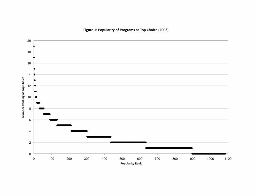
0

2

4

6

8

10

12

14

16

18

20

0 100 200 300 400 500 600 700 800 900 1000 1100

Num

berRa

nkingasTop

Cho

ice

PopularityRank

Figure1:PopularityofProgramsasTopChoice(2003)

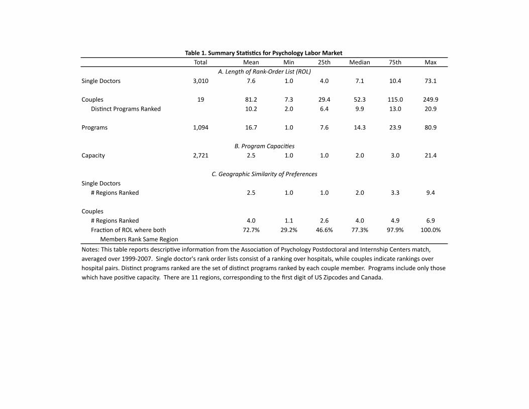
Total Mean Min 25th Median 75th Max

SingleDoctors 3,010 7.6 1.0 4.0 7.1 10.4 73.1

Couples 19 81.2 7.3 29.4 52.3 115.0 249.9DisCnctProgramsRanked 10.2 2.0 6.4 9.9 13.0 20.9

Programs 1,094 16.7 1.0 7.6 14.3 23.9 80.9

Capacity 2,721 2.5 1.0 1.0 2.0 3.0 21.4

SingleDoctors#RegionsRanked 2.5 1.0 1.0 2.0 3.3 9.4

Couples#RegionsRanked 4.0 1.1 2.6 4.0 4.9 6.9FracConofROLwhereboth 72.7% 29.2% 46.6% 77.3% 97.9% 100.0%MembersRankSameRegion

C.GeographicSimilarityofPreferences

Table1.SummarySta/s/csforPsychologyLaborMarket

A.LengthofRank‐OrderList(ROL)

B.ProgramCapaciAes

Notes:ThistablereportsdescripCveinformaConfromtheAssociaConofPsychologyPostdoctoralandInternshipCentersmatch,averagedover1999‐2007.Singledoctor'srankorderlistsconsistofarankingoverhospitals,whilecouplesindicaterankingsoverhospitalpairs.DisCnctprogramsrankedarethesetofdisCnctprogramsrankedbyeachcouplemember.ProgramsincludeonlythosewhichhaveposiCvecapacity.Thereare11regions,correspondingtothefirstdigitofUSZipcodesandCanada.

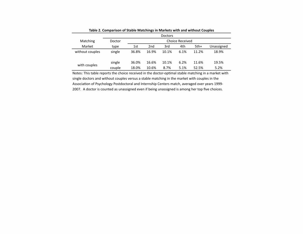
Matching DoctorMarket type 1st 2nd 3rd 4th 5th+ Unassigned

withoutcouples single 36.8% 16.9% 10.1% 6.1% 11.2% 18.9%

single 36.0% 16.6% 10.1% 6.2% 11.6% 19.5%couple 18.0% 10.6% 8.7% 5.1% 52.5% 5.2%

Table2.ComparisonofStableMatchingsinMarketswithandwithoutCouples

Notes:Thistablereportsthechoicereceivedinthedoctor‐opJmalstablematchinginamarketwithsingledoctorsandwithoutcouplesversusastablematchinginthemarketwithcouplesintheAssociaJonofPsychologyPostdoctoralandInternshipCentersmatch,averagedoveryears1999‐2007.Adoctoriscountedasunassignedevenifbeingunassignedisamonghertopfivechoices.

ChoiceReceived

withcouples

Doctors

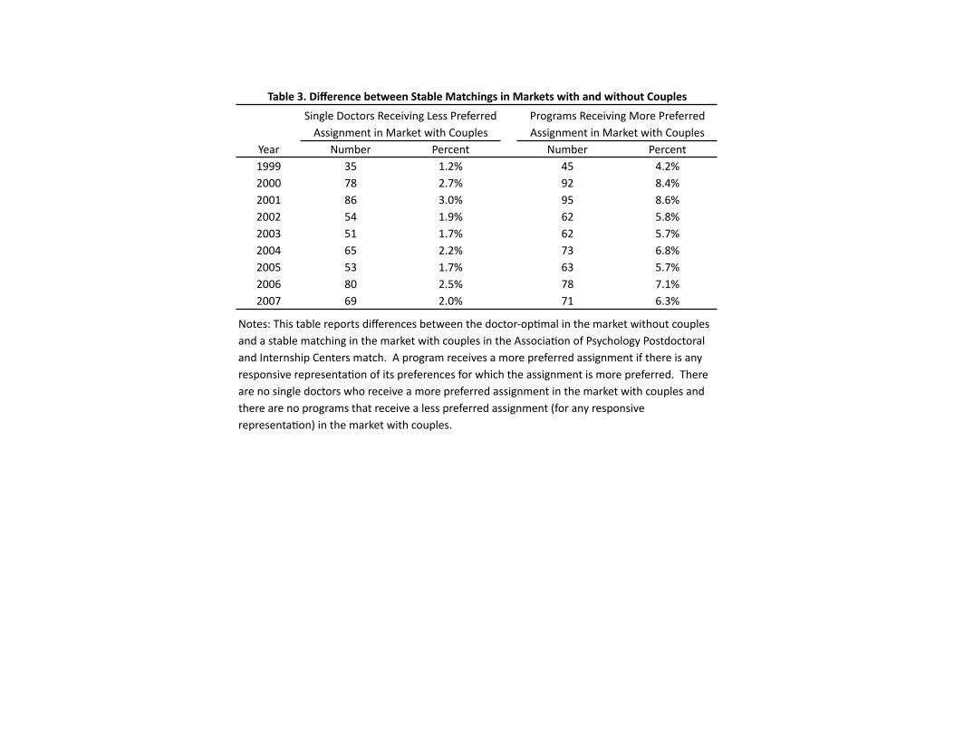
Year Number Percent Number Percent1999 35 1.2% 45 4.2%2000 78 2.7% 92 8.4%2001 86 3.0% 95 8.6%2002 54 1.9% 62 5.8%2003 51 1.7% 62 5.7%2004 65 2.2% 73 6.8%2005 53 1.7% 63 5.7%2006 80 2.5% 78 7.1%2007 69 2.0% 71 6.3%

SingleDoctorsReceivingLessPreferredAssignmentinMarketwithCouples

ProgramsReceivingMorePreferredAssignmentinMarketwithCouples

Table3.DifferencebetweenStableMatchingsinMarketswithandwithoutCouples

Notes:Thistablereportsdifferencesbetweenthedoctor‐opQmalinthemarketwithoutcouplesandastablematchinginthemarketwithcouplesintheAssociaQonofPsychologyPostdoctoralandInternshipCentersmatch.AprogramreceivesamorepreferredassignmentifthereisanyresponsiverepresentaQonofitspreferencesforwhichtheassignmentismorepreferred.Therearenosingledoctorswhoreceiveamorepreferredassignmentinthemarketwithcouplesandtherearenoprogramsthatreceivealesspreferredassignment(foranyresponsiverepresentaQon)inthemarketwithcouples.

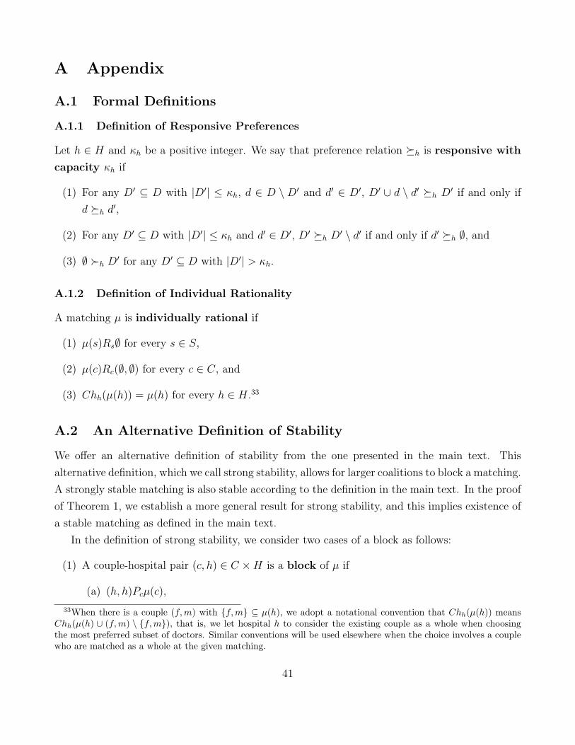
A Appendix

A.1 Formal Definitions

A.1.1 Definition of Responsive Preferences

Let h ∈ H and κh be a positive integer. We say that preference relation �h is responsive with

capacity κh if

(1) For any D′ ⊆ D with |D′| ≤ κh, d ∈ D \ D′ and d′ ∈ D′, D′ ∪ d \ d′ �h D′ if and only if

d �h d′,

(2) For any D′ ⊆ D with |D′| ≤ κh and d′ ∈ D′, D′ �h D′ \ d′ if and only if d′ �h ∅, and

(3) ∅ �h D′ for any D′ ⊆ D with |D′| > κh.

A.1.2 Definition of Individual Rationality

A matching µ is individually rational if

(1) µ(s)Rs∅ for every s ∈ S,

(2) µ(c)Rc(∅, ∅) for every c ∈ C, and

(3) Chh(µ(h)) = µ(h) for every h ∈ H.33

A.2 An Alternative Definition of Stability

We offer an alternative definition of stability from the one presented in the main text. This

alternative definition, which we call strong stability, allows for larger coalitions to block a matching.

A strongly stable matching is also stable according to the definition in the main text. In the proof

of Theorem 1, we establish a more general result for strong stability, and this implies existence of

a stable matching as defined in the main text.

In the definition of strong stability, we consider two cases of a block as follows:

(1) A couple-hospital pair (c, h) ∈ C ×H is a block of µ if

(a) (h, h)Pcµ(c),

33When there is a couple (f,m) with {f,m} ⊆ µ(h), we adopt a notational convention that Chh(µ(h)) meansChh(µ(h) ∪ (f,m) \ {f,m}), that is, we let hospital h to consider the existing couple as a whole when choosingthe most preferred subset of doctors. Similar conventions will be used elsewhere when the choice involves a couplewho are matched as a whole at the given matching.

41

(b) f,m ∈ Chh(µ(h) ∪ c) where c = (f,m).

(2) A group of doctors D′ and hospital h is a block of µ if

(a) there is no couple (f,m) such that {f,m} ⊆ D′,

(b) D′ ⊆ Chh(µ(h) ∪D′),34

(c) for all s ∈ D′ ∩ S, we have hPsµ(s),

(d) i. for all f ∈ D′ ∩ F where c = (f,m) ∈ C, (h, h′)Pcµ(c) for some h′ and m ∈Chh′(µ(h′) ∪m),

ii. for all m ∈ D′ ∩M where c = (f,m) ∈ C, we have (h′, h)Pcµ(c) for some h′ and

f ∈ Chh′(µ(h′) ∪ f).

A matching is strongly stable if it is individually rational and there is no block as defined by

conditions (1) and (2) above.

This definition allows for a couple assigned to a hospital to be blocked by two doctors (who

are either single or are a member of a couple). If one of the blocking doctors is a couple member,

we require that the member’s partner is chosen by another hospital over its assignment and that

the couple together prefer this assignment to their current assignment.

The motivation for this definition is to allow certain joint deviations to happen, but rule out

more complicated deviations involving larger groups. When a couple member is part of a blocking

coalition of doctors D′ and hospital h, our interpretation is that hospital h is the “initiating”

blocker, and any hospital h′ involved to satiate the other member of a couple is a passive blocker.

The reason we consider this definition is to stay close to pairwise stability, but still accommodate

this particular type of blocking pair is that we think that blocking coalitions of larger size are less

likely to form due to coordination issues among members. This definition also keeps the notation

less burdensome, but our main existence result continues to hold when we allow larger sets of

blocking coalitions to form or employ the core as our solution concept.

Since the definition of strong stability allows for coalitions of doctors who are single or couple

members to be part of blocking pairs, a strongly stable matching is stable, but not vice versa.

Moreover, if each hospital has one position, strong stability is equivalent to unit-capacity stability.

Finally, strong stability is equivalent to the standard definition of (pairwise) stability when

there is no couple. To see this last point, first observe that condition (1) in the definition of strong

34When there is a couple (f,m) with {f,m} ⊆ µ(h), then we adopt a notational convention that Chh(µ(h)∪D′)means Chh(µ(h) ∪ (f,m) \ {f,m} ∪ D′), that is, we let hospital h consider the existing couple as a whole whenchoosing the most preferred subset of doctors. A similar convention will be used elsewhere when the choice involvesa couple who are matched as a whole at the given matching.

42

stability is irrelevant if there is no couple, as are conditions (2a) and (2d). The remaining condi-

tions (2b) and (2c) are equivalent to the nonexistence of a blocking pair under the assumption that

hospital preferences are responsive. Thus this, together with individual rationality, is equivalent

to the standard pairwise stability concept.

A.3 Proof of Theorem 1

Let (H,S,C, (�h)h∈H , (Ri)i∈S∪C) be a matching market.

Step 1: Doctor-Proposing Deferred Acceptance Algorithm

Apply the doctor-proposing deferred acceptance algorithm to the sub-market without couples:

(H,S, (�h)h∈H , (Rs)s∈S).

Step 2: Sequential Couples Algorithm

Algorithm 2. Sequential Couples Algorithm

(1) Initialization:

Let matching µ be the output of the deferred acceptance algorithm in the sub-market without

couples.

(2) Iterate through couples : set C0 = C, i = 0 and B = ∅.

(a) If Ci is empty, then go to Step 3. Otherwise, pick some couple c = (f,m) ∈ Ci. Let

Ci+1 = Ci\c and increment i by one.

(b) Let couple c apply to their most preferred pair of hospitals (h, h′) ∈ H × H that has

not rejected them yet.

i. If such a hospital (pair) does not exist, modify matching µ such that couple c is

unassigned and then go to Step 2a.

ii. If such a hospital (pair) exists, then if either hospital h or hospital h′ has previously

been applied to by a member (or both members) of any couple different from c,

then terminate the algorithm.

iii. Otherwise,

43

A. If h = h′ 6= ∅ and {f,m} ⊆ Chh(µ(h)∪c), then modify matching µ by assigning

(f,m) to hospital h and having h reject

(µ(h) ∪ f ∪m) \ Chh(µ(h) ∪ c).

Add the rejected single doctors (if any) to B and go to Step 2a.

B. If h 6= h′, f ∈ Chh(µ(h)∪ f), and m ∈ Chh′(µ(h′)∪m), then modify matching

µ by assigning f to h and m to h′, having hospital h reject

(µ(h) ∪ f) \ Chh(µ(h) ∪ f),

and having hospital h′ reject

(µ(h′) ∪m) \ Chh′(µ(h′) ∪m).

Add the rejected single doctors (if any) to B and go to Step 2a.

C. Otherwise, let hospital h and hospital h′ reject the application by couple c and

go to Step 2b.

(3) Iterate through rejected single doctors : set B1 = B and j = 1.

Round j:

(a) If Bj is empty, then terminate the algorithm.

(b) Otherwise, pick some single doctor s in Bj. Let Bj+1 = Bj\s and increment j by one.

Iterate through the rank order lists of single doctors:

i. If single doctor s has applied to every acceptable hospital, then modify matching

µ such that s is unassigned and go to Step 3a.

ii. If not, then let h be the most preferred hospital ranked by single doctor s among

those which s has not yet applied to previously (either in the doctor-proposing

deferred acceptance algorithm or within this algorithm.)

iii. If there is no couple member who has ever applied to hospital h, then there are

three cases:

A. If hospital h has a vacant position and s is acceptable to h, then modify match-

ing µ such that single doctor s is assigned to h and go to Step 3a.

44

B. If either hospital h prefers each of its current mates to single doctor s and there

is no vacant position or s is unacceptable to h, then h rejects s and go to Step

3(b)i.

C. If hospital h prefers single doctor s to one of its current mates and there is no

vacant position, then modify matching µ such that s is assigned to h. Hospital

h rejects the least preferred doctor currently assigned there:

(µ(h) ∪ s) \ Chh(µ(h) ∪ s).

With abuse of notation, denote this rejected doctor s and go to Step 3(b)i.

iv. If there is a couple member who has ever applied to hospital h previously within

this algorithm, then terminate the algorithm.

The sequential couples algorithm terminates at Step 2(b)ii (when a couple member proposes to

a hospital which has already been proposed to by another couple), Step 3a (when all couples and

single doctors are assigned), or Step 3(b)iv (when a single doctor proposes to a hospital which was

previously applied to by a couple member). We say that the algorithm succeeds if it terminates

at Step 3a.

Lemma 1. If the sequential couples algorithm succeeds, then the resulting matching is stable.

The proof of this lemma is similar to the proof of the existence of a stable matching by Gale and

Shapley (1962) in the college admissions model. The main difference is that when the sequential

couples algorithm succeeds, we must verify that there are no blocking pairs including pairs which

may involve members of a couple.

Proof of Lemma 1. We prove that the matching that results when the sequential couples algorithm

succeeds is strongly stable (defined in Section A.2). Establishing this fact implies that the matching

is stable since a strongly stable matching is a stable matching.35

Suppose that Algorithm 2 succeeds, producing matching µ. First, µ is individually rational

since all doctors who are single or couple members have applied only to acceptable hospitals

(hospital pairs for couples), and hospitals have accepted only acceptable doctors only up to their

capacities in each step of Algorithms 1 and 2.

Next, to show that there is no block of matching µ, fix a hospital h ∈ H \ ∅.

(1) Suppose that there exists no couple (f,m) ∈ C such that {f,m} ⊆ µ(h).

35Since the rest of the analysis builds on this lemma, this stronger result allows us to extend our main resultswhen we replace stability with strong stability as the solution concept.

45

(a) Assume, for contradiction, that there exists a set of doctors D′ ⊆ D such that hospital

h and D′ block µ, where there is no couple (f,m) ∈ C such that {f,m} ⊆ D′. Since

doctor d is part of a block,

dPh∅ for every d ∈ D′.

There are two cases to consider depending on whether D′ contains any single doctors.

i. Suppose that there is a single doctor in D′. Then each single doctor s ∈ D′ ∩ Sis rejected by hospital h at some point of either Algorithm 1 or 2 since hPsµ(s).

The tentative assignment of hospital h at a step when single doctor s is rejected,

denoted µ(h), satisfies

|µ(h)| = κh and dPhs for all d ∈ µ(h),

because sPh∅. Since, at each of later steps of both Algorithms, hospital h replaces

a tentatively matched doctor only when a more preferred doctor applies, it follows

that

|µ(h)| = κh and dPhs for all d ∈ µ(h).

This contradicts the assumption that hospital h and D′ block matching µ.

ii. Suppose there are no single doctors in D′. Then there exists a member of some

couple in D′. Without loss of generality, assume that there is some f ∈ D′ where

c = (f,m) ∈ C. Since (h, h′)Pcµ(c) for some h′ ∈ H, couple c was rejected by

the hospital pair (h, h′) at some point of Algorithm 2. Let µ(h) and µ(h′) be

the tentative assignments for hospital h and hospital h′ at that step, respectively.

Because couple c was rejected at this step, it follows that either

|µ(h)| = κh and dPhf for all d ∈ µ(h),

or h′ 6= ∅ and we have that

|µ(h′)| = κh′ and dPh′m for all d ∈ µ(h′).

Since, at each of later steps, both hospital h and hospital h′ (if h′ 6= ∅) replace a

tentatively matched doctor only when a more preferred doctor applies, it follows

46

that either

|µ(h)| = κh and dPhf for all d ∈ µ(h),

or h′ 6= ∅ and we have that

|µ(h′)| = κh′ and dPh′m for all d ∈ µ(h′).

This contradicts the assumption that f ∈ D′ and D′ block matching µ with hospital

h.

(b) Consider a couple c = (f,m) such that (h, h)Pcµ(c). By definition of Algorithm 2, the

couple was rejected by the hospital pair (h, h) at some point in the Algorithm. Denote

the matching at that point by µ. It follows that

Chh(µ(h) ∪ c) = µ(h) and f,m /∈ µ(h).

Since the sequential couples algorithm succeeds, no other doctor applies to hospital h

after the step where couple c is rejected by (h, h). As a result,

µ(h) = µ(h).

Therefore,

f,m /∈ µ(h) and µ(h) = Chh(µ(h) ∪ c),

which contradicts the assumption that couple c and hospital h block matching µ.

(2) Suppose that there exists a couple (f,m) ∈ C such that {f,m} ⊆ µ(h) and there is a block

of matching µ involving hospital h. The assumption that the sequential couples algorithm

succeeds implies that there is no couple c 6= (f,m) and h′ ∈ H such that (h, h′)Pcµ(c) or

(h′, h)Pcµ(c). This is because the algorithm terminates in Step 3 if two or more distinct

couple members apply to the same hospital during the algorithm. Thus, the set of doctors

D′ that blocks matching µ with hospital h is composed solely of single doctors. This means

that

sPh∅ for every s ∈ D′, (1)

hPsµ(s) for every s ∈ D′, (2)

for otherwise a single doctor s is not part of a block. Let µ be the matching that is the result

47

of the doctor-proposing deferred acceptance algorithm in the sub-market excluding couples.

Then

hRsµ(s) for every s ∈ D′, (3)

because otherwise, in light of (2), single doctor s will have applied to hospital h in Step 3 of

the sequential couples algorithm, causing the algorithm to fail. Moreover,

µ(h) �h µ(h), (4)

because otherwise hospital h would not have accepted new applicants in Step 2 of the

sequential couples algorithm, resulting in matching with µ(h). Furthermore,

dPhs for every d ∈ µ(h) ∩ µ(h) and s ∈ D′, (5)

because

(a) for any s ∈ D′ ∩ µ(h), single doctor s was rejected in Step 2 of the sequential couples

algorithm at the instance when the couple (f,m) applied to hospital h. We now show

dPhs. Suppose, to the contrary, that sRhd for some d ∈ µ(h)∩µ(h). Then sPhd because

s 6= d and preferences are strict. This relation and responsiveness of �h imply

µ(h) ∪ s \ d �h µ(h).

Moreover,

µ(h) ∪ s \ d ∈ A(µ(h) ∪ (f,m)).

These facts contradict

µ(h) = Chh(µ(h) ∪ (f,m)),

which follows from the definition of the sequential couples algorithm. Hence,

dPhs for all d ∈ µ(h) ∩ µ(h).

(b) for any s ∈ D′\ µ(h), relation (3) implies hPsµ(s), so stability of matching µ in the sub-

market without couples (which coincides with both our stability definition in Section

48

3.1 and strong stability definition in Appendix A.2) implies

dPhs for all d ∈ µ(h).

Let µ′(h) be the assignment for hospital h when D′ and hospital h block matching µ. That

is,

µ′(h) = Chh(µ(h) ∪D′). (6)

Relation (6) and the definition of Chh(·) imply

µ′(h) �h µ(h). (7)

Relations (1) and (2) imply that

|µ(h)| = κh.

Therefore, to block matching µ with D′, hospital h should reject some doctors in µ(h). If

any doctor d ∈ µ(h)∩ µ(h) is rejected while some s ∈ D′ is accepted to produce µ′(h), then

µ′(h) ∪ d \ s �h µ′(h)

by responsiveness of �h and relation (5), but this contradicts (6). Hence, relation (5) implies

that it should be exactly couple (f,m) that is rejected by hospital h when hospital h and

D′ block µ(h). Since (f,m) is the only couple in µ(h) and it is not in µ′(h),

µ′(h) ⊆ µ(h) ∪D′ ⊆ S.

Since hRsµ(s) for every single doctor s ∈ µ′(h) by relation (3) and µ′(h) ⊆ S, it follows that

µ(h) �h µ′(h), (8)

because otherwise matching µ would be unstable in the sub-market without couples. Ap-

plying relations (4), (8), and then (7), we obtain

µ(h) �h µ(h) �h µ′(h) �h µ(h),

a contradiction.

49

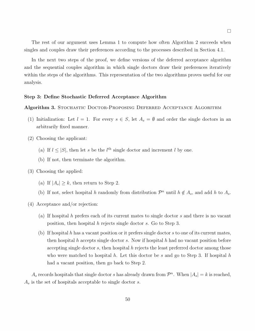
The rest of our argument uses Lemma 1 to compute how often Algorithm 2 succeeds when

singles and couples draw their preferences according to the processes described in Section 4.1.

In the next two steps of the proof, we define versions of the deferred acceptance algorithm

and the sequential couples algorithm in which single doctors draw their preferences iteratively

within the steps of the algorithms. This representation of the two algorithms proves useful for our

analysis.

Step 3: Define Stochastic Deferred Acceptance Algorithm

Algorithm 3. Stochastic Doctor-Proposing Deferred Acceptance Algorithm

(1) Initialization: Let l = 1. For every s ∈ S, let As = ∅ and order the single doctors in an

arbitrarily fixed manner.

(2) Choosing the applicant:

(a) If l ≤ |S|, then let s be the lth single doctor and increment l by one.

(b) If not, then terminate the algorithm.

(3) Choosing the applied:

(a) If |As| ≥ k, then return to Step 2.

(b) If not, select hospital h randomly from distribution Pn until h /∈ As, and add h to As.

(4) Acceptance and/or rejection:

(a) If hospital h prefers each of its current mates to single doctor s and there is no vacant

position, then hospital h rejects single doctor s. Go to Step 3.

(b) If hospital h has a vacant position or it prefers single doctor s to one of its current mates,

then hospital h accepts single doctor s. Now if hospital h had no vacant position before

accepting single doctor s, then hospital h rejects the least preferred doctor among those

who were matched to hospital h. Let this doctor be s and go to Step 3. If hospital h

had a vacant position, then go back to Step 2.

As records hospitals that single doctor s has already drawn from Pn. When |As| = k is reached,

As is the set of hospitals acceptable to single doctor s.

50

Let µ be the matching that is produced when Algorithm 3 terminates. Under the doctor

proposing deferred acceptance algorithm, a single doctor’s application to her tth most preferred

hospital is independent of her preferences after (t+ 1)th choice on. Therefore matching µ is stable

for the market consisting of single doctors, any of their realized preference profiles which could

follow from completing the draws for random preferences, the hospitals and their (arbitrarily fixed)

preferences.

Step 4: Define Stochastic Sequential Couples Algorithm

Suppose that at the conclusion of Algorithm 3, we obtain matching µ. The stochastic sequen-

tial couples algorithm is a version of Algorithm 2 where single doctor preferences are drawn

iteratively, and is defined as follows:

Algorithm 4. Stochastic Sequential Couples Algorithm

(1) Initialization:

(a) Keep all preference lists generated in Algorithm 3. Also, for each single doctor s ∈ S,

let As be the set generated at the end of Algorithm 3. Let the matching µ be the initial

matching of the algorithm.

(b) For each couple c = (f,m) ∈ C, construct the couples’ preferences Pc according to the

process defined in Section 4.1.

(2) Iterate through couples, set C0 = C, i = 0, and B = ∅.

(a) If Ci is empty, then go to Step 3. Otherwise, pick some couple c = (f,m) ∈ Ci. Let

Ci+1 = Ci\c and increment i by one.

(b) Let couple c apply to their most preferred pair (h, h′) ∈ H ×H that has not rejected

them yet.

i. If such a hospital (pair) does not exist, modify matching µ such that couple c is

unassigned and then go to Step 2a.

ii. If such a hospital (pair) exists, then if either hospital h or hospital h′ has previously

been applied to by a member (or both members) of any couple different from c,

then terminate the algorithm.

iii. Otherwise,

51

A. If h = h′ 6= ∅ and {f,m} ⊆ Chh(µ(h)∪c), then modify matching µ by assigning

(f,m) to hospital h and having h reject

(µ(h) ∪ f ∪m) \ Chh(µ(h) ∪ c).

Add the rejected single doctors (if any) to B and go to Step 2a.

B. If h 6= h′, f ∈ Chh(µ(h)∪ f), and m ∈ Chh′(µ(h′)∪m), then modify matching

µ by assigning f to h and m to h′, having hospital h reject

(µ(h) ∪ f) \ Chh(µ(h) ∪ f),

and having hospital h′ reject

(µ(h′) ∪m) \ Chh′(µ(h′) ∪m).

Add the rejected single doctors (if any) to B and go to Step 2a.

C. Otherwise, let hospital h and hospital h′ reject the application by couple c and

go to Step 2b.

(3) Iterate through rejected single doctors, set B1 = B and j = 1.

Round j:

(a) If Bj is empty, then terminate the algorithm.

(b) Otherwise, pick some single doctor s in Bj. Set Bj+1 = Bj\s and increment j by one.

Iterate through the single doctor’s rank order list (call this iteration “Round j”)

i. If |As| ≥ k, then go to Step 3a.

ii. If not, select hospital h randomly from distribution Pn until h 6∈ As, and add h to

As.

iii. If there is no couple member who has ever applied to hospital h, then there are

three cases:

A. If hospital h has a vacant position, then modify matching µ such that single

doctor s is assigned to h and go to Step 3a.

B. If either hospital h prefers each of its current mates to single doctor s and there

is no vacant position or s is unacceptable to h, then h rejects s and go to Step

3(b)i.

52

C. If hospital h prefers single doctor s to one of its current mates and there is no

vacant position, then modify matching µ such that s is assigned to h. Hospital

h rejects the least preferred doctor currently assigned there

(µ(h) ∪ s) \ Chh(µ(h) ∪ s).

With abuse of notation, denote this rejected doctor s and iterate through her

rank order list by going to Step 3(b)i.

iv. If there is a couple member who has ever applied to hospital h before, then termi-

nate the algorithm.

The algorithm above terminates at Step 2(b)ii or Step 3a or Step 3(b)iv. Similarly to Algorithm

2, we say that Algorithm 4 succeeds if it terminates at Step 3a.

To establish Theorem 1, we investigate how often the algorithm succeeds, as single doctors

draw hospitals from distribution Pn and couples draw hospitals from Qn. First observe for any

random market in a regular sequence,

Pr[Algorithm 2 succeeds] = Pr[Algorithm 4 succeeds].

That is, the probability of the algorithm’s success is identical whether random preferences

are drawn at once in the beginning or they are drawn one at a time during the execution of the

algorithm.36 The latter expression is useful since we can investigate the procedure step by step,

utilizing conditional probabilities and conditional expectations. Thus we focus on the behavior of

Algorithm 4 as the market size grows in the remainder of the proof.

Let Yn be a random variable which counts the number of hospitals that are listed on no single

doctor’s preference list at the end of Algorithm 3.37 The next step of the argument provides a

lower bound on Yn at the conclusion of Algorithm 3.

Step 5: A large number of hospitals have vacancies

Lemma 2. For any n > 4k,

E[Yn] ≥ n

2e−16λk.

36This property is called the principle of deferred decisions. See Motwani and Raghavan (1996).37We abuse notation and denote a random variable and its realization by the same letter when there is no

confusion.

53

Proof. We order the hospitals in terms of decreasing popularity with respect to Pn: label H =

{h1, h2, . . . , hn} with ph` ≥ ph`+1for all ` ∈ {1, . . . , n− 1}. If hospitals have equal popularity, we

order them in some fixed manner. Let the probability mass for the first k hospitals be:

π =k∑`=1

ph` .

Fix a single doctor and denote her ith most preferred hospital by h(i), if it has been drawn at

the conclusion of Algorithm 3. For any i ≤ k, the definition of π implies

i−1∑j=1

ph(j)≤ π.

Thus for any i ≤ k, the conditional probability that h is not the single doctor’s ith choice given

the events that her first (i− 1) choices are h(1), . . . , h(i−1), her ith choice is drawn, and h(j) 6= h for

all j ≤ i− 1, is bounded from below by

1− ph

1−∑i−1

j=1 ph(j)

≥ 1− ph1− π

. (9)

Let Eh be the event that h /∈ As for every s ∈ S at the end of Algorithm 3. Since at most λnk

draws are made in total by all single doctors from Pn in Algorithm 3, inequality (9) implies that

Pr(Eh) ≥(

1− ph1− π

)λnk. (10)

If hospital index ` > k, there are at least `− k hospitals in H \ {h1, . . . , hk} that are at least

as popular as h` according to Pn, so we obtain

π + (`− k)ph` ≤ 1

⇐⇒ ph` ≤ 1−π`−k . (11)

The last two inequalities, (10) and (11), imply

Pr(Eh`) ≥(

1− 1

`− k

)λnk. (12)

54

We next show that for any ` > 2k,(1− 1

`− k

)λnk≥ e−2λnk/(`−k). (13)

To see that (13) holds, first note that

(1− 1

`− k

)λnk≥ e−2λnk/(`−k) ⇐⇒ 1− 1

`− k− e−2/(`−k) ≥ 0.

Now, define a function g(x) = 1 − x − e−2x. This function g is concave, and g(0) = 0 and

g(1/2) = 1/2 − 1/e > 0. Therefore g(x) ≥ 0 for any x ∈ [0, 1/2]. Since ` > 2k and k is a

positive integer, we have `− k > k ≥ 1. Since `− k is an integer, we obtain `− k ≥ 2 and hence

1/(`− k) ∈ [0, 1/2]. Therefore

1− 1/(`− k)− e−2/(`−k) = g(1/(`− k)) ≥ 0,

establishing inequality (13).

Moreover, for any ` > 2k,

e−2λnk/(`−k) ≥ e−4λnk/`. (14)

Combining inequalities (12), (13), and (14), we obtain:

Pr(Eh`) ≥ e−4λnk/`.

Using this inequality, for any n > 4k, we have

E[Yn] =n∑`=1

Pr(Eh`) ≥n∑

`=2k

e−4λnk/` ≥n∑

`=bn/2c+1

e−8λnk/` ≥ n

2e−16λk,

where bxc is the largest integer not greater than x.

Step 6: Algorithm 4 succeeds with high probability.

Let C = bna denote the upper bound on the number of couples in the random market Γn.

55

Lemma 3. For any sufficiently large n and any matching µ,

Pr

[Algorithm 4 succeeds

∣∣∣∣ Yn > E[Yn]

2and Algorithm 3 produces µ

]≥(

1− 2kCr

n

)2kC

·(

1− 8rkC

E[Yn]

)2C

,

if the conditioning event has a strictly positive probability.

Proof. First, consider the event that Algorithm 4 does not terminate at Step 2(b)ii so that the

algorithm reaches Step 3. For that event to happen it is enough for the following event to happen:

for any two doctors d, d′ ∈ F ∪M with d 6= d′, there is no hospital h ∈ H that is listed by both

d and d′ as an acceptable hospital. This is sufficient because our assumption on ρ implies that at

most one couple member will apply to h.

Suppose {d1, ..., d`−1} ∈ F ∪M are such that there exists no h ∈ H listed by any pair of doctors

in {d1, ..., d`−1} ∈ F ∪M . Furthermore, fix a doctor d` ∈ F ∪M \ {d1, ..., d`−1} and assume that

her first i− 1 choices {h(1), h(2), . . . , h(i−1)} have no intersection with hospitals listed by the set of

doctors {d1, ..., d`−1}. The conditional probability that her ith choice h(i) does not have an overlap

with any of the previously picked hospital is at least

1−∑

h:h is listed by some doctor in {d1,...,d`−1}

qh −i−1∑j=1

qh(j). (15)

Condition (4) of Definition 1 implies that

qh ≤ rqh′ for all h, h′ ∈ H.

Adding these inequalities across hospitals h′ ∈ H, we have

nqh ≤ r∑h′∈H

qh′ for each h.

As a result,

qh ≤r∑

h′∈H qh′

n≤ r

n.

Since there are at most C couples and each member of a couple lists at most k distinct hospitals,

56

expression (15) is bounded from below by

1− 2kCr

n. (16)

Recall that there are at most C couples and each member of the couple lists at most k distinct

hospitals. Expression (16) implies that the probability that for any d, d′ ∈ F ∪M with d 6= d′,

there is no hospital h ∈ H that is listed by both d and d′ as one of their acceptable hospitals is at

least (1− 2kCr

n

)2kC

, (17)

which is positive for n sufficiently large. Expression (17) provides a lower bound of the probability

that the algorithm does not terminate at Step 2(b)ii so that the algorithm reaches Step 3.

Next, we consider what happens in Step 3 assigning single doctors in the set B, conditional on

the same events assumed so far and in addition that all couples are tentatively matched without

the algorithm being terminated at Step 2(b)ii.

Condition (4) of Definition 1 implies that

ph′ ≥ ph/r for any h, h′ ∈ H.

Also observe that there are at most 2kC hospitals that are listed by a couple member in F ∪M .

Denote this set of hospitals by H1 and note that∑h∈H1

qh ≤ 2kCr ·minh∈H{qh}.

Moreover, there are at least Yn − 2kC hospitals (which is positive if n is sufficiently large and

Yn >E[Yn]

2) with vacant positions and not listed by any couple member at the beginning of Step 3

(since there are at least Yn hospitals with vacant positions at the beginning of Step 2 and at most

2C hospitals are listed by couple members). Denote this set of hospitals by H2 and note that∑h∈H2

qh ≥ (Yn − 2kC) ·minh∈H{qh}.

We are interested in computing the probability that Round 1 of Step 3 ends at 3(b)iiiA as

a single doctor applies to some hospital with vacant positions not listed by any couple member

(rather than applying to a hospital that is listed by a couple member). This probability is bounded

57

below by:

1−∑

h∈H1qh∑

h∈H1qh +

∑h∈H2

qh≥ 1− 2kC

Yn−2kCr

+ 2kC> 1− 2kC

E[Yn]/2−2kCr

+ 2kC. (18)

Now assume that all Rounds 1, . . . , j − 1 end at Step 3(b)iiiA. Then there are still at least

Yn − 2kC − (j − 1) hospitals with a vacant position and not listed by any couple member at the

end of Round j − 1. This follows since at most j − 1 hospitals have had their positions filled at

Rounds 1, . . . , j − 1 among those hospitals that are not listed on any single doctor’s preference

list at the end of Algorithm 3. Following the steps analogous to those leading to inequality (18),

we can compute that Round j, initiated by some single doctor in Bj, ends at Step 3(b)iiiA with

probability of at least

1− 2kCYn−2kC−(j−1)

r+ 2kC

> 1− 2kCE[Yn]/2−2kC−(j−1)

r+ 2kC

.

There are at most 2C rounds in Step 3 because at most 2C single doctors can be displaced

by couples in Step 2, so |B| ≤ 2C. Hence Algorithm 4 succeeds with conditional probability of at

least

2C∏j=1

(1− 2kC

E[Yn]/2−2kC−(j−1)r

+ 2kC

)≥

(1− 2kC

E[Yn]/2−2kC−(2C−1)r

+ 2kC

)2C

≥(

1− 2kC

E[Yn]/4r

)2C

, (19)

where the first inequality follows from Lemma 2, the assumption that n is sufficiently large and

each j ≤ 2C, and the second inequality holds since E[Yn]/2− 4kC ≥ E[Yn]/4 > 0, which follows

from Lemma 2 and the assumption that n is sufficiently large.

As a result, relations (17) and (19) imply

Pr

[Algorithm 4 succeeds

∣∣∣∣ Yn > E[Yn]

2and Algorithm 3 produces µ

]≥(

1− 2kCr

n

)2kC

·(

1− 8rkC

E[Yn]

)2C

.

We utilize the following mathematical result (see Lemma 4.4 of Immorlica and Mahdian (2005)

58

for a proof).

Lemma 4. Var[Yn] ≤ E[Yn] for every n ∈ N.

Step 7: Proof of Theorem 1

Proof of Theorem 1. We obtain that

Pr

[Yn ≤

E[Yn]

2

]≤ Pr

[Yn ≤

E[Yn]

2

]+ Pr

[Yn ≥

3E[Yn]

2

]= Pr

[|Yn − E[Yn]| ≥ E[Yn]

2

]≤ Var[Yn]

(E[Yn]/2)2≤ 4

E[Yn], (20)

where the first inequality holds since any probability is nonnegative, the equality is an identity, the

second inequality results from Chebyshev inequality, and the last inequality follows from Lemma

4.

By Lemma 3 we have

Pr

[Algorithm 4 succeeds

∣∣∣∣ Yn > E[Yn]

2and Algorithm 3 produces µ

]≥(

1− 2kCr

n

)2kC

·(

1− 8rkC

E[Yn]

)2C

.

This inequality holds for any matching µ that is produced at the end of Algorithm 3. Therefore,

we have the same lower bound for the probability conditional on Yn > E[Yn]/2 but not on µ. That

is,

Pr

[Algorithm 4 succeeds

∣∣∣∣ Yn > E[Yn]

2

]≥(

1− 2kCr

n

)2kC

·(

1− 8rkC

E[Yn]

)2C

. (21)

Thus we obtain

Pr [Algorithm 4 succeeds] ≥ Pr

[Yn >

E[Yn]

2

]·(

1− 2kCr

n

)2kC

·(

1− 8rkC

E[Yn]

)2C

≥(

1− 4

E[Yn]

)·(

1− 2kCr

n

)2kC

·(

1− 8rkC

E[Yn]

)2C

≥(

1− 8e16λk

n

)·(

1− 2kCr

n

)2kC

·(

1− 16rkCe16λk

n

)2C

, (22)

where the first inequality follows from the fact that probabilities are non-negative and (21), the

59

second inequality results from (20), and the last inequality is obtained by Lemma 2.

The first term on the right-hand side of inequality (22),(

1− 8e16λk

n

), converges to one as long

as n→∞. Consider the second term,(

1− 2kCrn

)2kC

. Recall there exists b > 0 such that C < bna

for any n. Thus, for any n,

(1− 2kCr

n

)2kC

>

(1− 2kbnar

n

)2kbna

=

(1− 2kbr

n1−a

)2kbn1−an2a−1

≥ (e−2kbr)2kbn2a−1

. (23)

where the last line follows from the inequality that(1− α

x

)x ≥ e−α when x, α > 0. Since

a ∈ [0, 1/2), the term n2a−1 → 0 as n → ∞ and hence the last expression of inequality (23)

converges to one as n → ∞. Similarly, the third term of the right-hand side of inequality (22),(1− 16rkCe16λk

n

)2C

, can be bounded as

(1− 16rkCe16λk

n

)2C

>

(1− 16rkbnae16λk

n

)2bna

=

(1− 16rkbe16λk

n1−a

)2bn1−an2a−1

≥ (e−16rkbe16λk)2bn2a−1

. (24)

Because a ∈ [0, 1/2), the last expression of inequality (24) converges to one as n → ∞, which

concludes the proof.

Speed of convergence Suppose that the number of couples is bounded along the sequence of

random markets (which is equivalent to a = 0 in the definition of a regular market). By inequality

(22), the probability that there does not exist a stable matching decreases with rate of convergence

of O(1/n) as n→∞. It is an open question whether this rate of convergence is tight.

Number of vacancies Since the proof of Theorem 1 finds a bound of the probability by focusing

on the event in which Yn >E[Yn]

2≥ n

4e−16λk, the following claim follows immediately.

Proposition 1 (A large number of hospitals with vacancies). There exists a constant β > 0 such

that

60

(1) the probability that, in a sub-market without couples, the doctor-proposing deferred acceptance

algorithm produces a matching in which at least βn hospitals have at least one vacant position

converges to one as n approaches infinity, and

(2) the probability that the sequential couples algorithm succeeds and at least βn hospitals have at

least one vacant position in the resulting matching converges to one as n approaches infinity.

A.4 Proof of Theorem 2

We consider incentives for single doctors, couples, and hospitals in the following subsections and

then combine the results to obtain the proof of Theorem 2. Let Pr[E] be the probability of the

event E.

A.4.1 Definition of the mechanism ϕ

Algorithm 5. Mechanism ϕ

(1) Initialization:

Let matching µ be the output of the deferred acceptance algorithm in the sub-market without

couples. Set C0 = C, B0 = ∅, i = 0.

(2) Iterate through couples :

(a) If Ci is empty, then go to Step 3. Otherwise, pick some couple c = (f,m) ∈ Ci

according to some prespecified deterministic rule. Let Ci+1 = Ci\c and Bi+1 = Bi, and

increment i by one.

(b) Let couple c apply to their most preferred pair of hospitals (h, h′) ∈ H × H that has

not rejected them yet.

i. If such a hospital (pair) does not exist, modify matching µ such that couple c is

unassigned and then go to Step 2a.

ii. If such a hospital (pair) exists,

A. If h = h′ 6= ∅ and {f,m} ⊆ Chh(µ(h)∪c), then modify matching µ by assigning

(f,m) to hospital h and having h reject

(µ(h) ∪ f ∪m) \ Chh(µ(h) ∪ c).

61

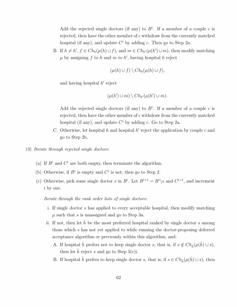
Add the rejected single doctors (if any) to Bi. If a member of a couple c is

rejected, then have the other member of c withdraw from the currently matched

hospital (if any), and update Ci by adding c. Then go to Step 2a.

B. If h 6= h′, f ∈ Chh(µ(h)∪ f), and m ∈ Chh′(µ(h′)∪m), then modify matching

µ by assigning f to h and m to h′, having hospital h reject

(µ(h) ∪ f) \ Chh(µ(h) ∪ f),

and having hospital h′ reject

(µ(h′) ∪m) \ Chh′(µ(h′) ∪m).

Add the rejected single doctors (if any) to Bi. If a member of a couple c is

rejected, then have the other member of c withdraw from the currently matched

hospital (if any), and update Ci by adding c. Go to Step 2a.

C. Otherwise, let hospital h and hospital h′ reject the application by couple c and

go to Step 2b.

(3) Iterate through rejected single doctors :

(a) If Bi and Ci are both empty, then terminate the algorithm.

(b) Otherwise, if Bi is empty and Ci is not, then go to Step 2.

(c) Otherwise, pick some single doctor s in Bi. Let Bi+1 = Bi\s and Ci+1, and increment

i by one.

Iterate through the rank order lists of single doctors:

i. If single doctor s has applied to every acceptable hospital, then modify matching

µ such that s is unassigned and go to Step 3a.

ii. If not, then let h be the most preferred hospital ranked by single doctor s among

those which s has not yet applied to while running the doctor-proposing deferred

acceptance algorithm or previously within this algorithm, and:

A. If hospital h prefers not to keep single doctor s, that is, if s /∈ Chh(µ(h) ∪ s),then let h reject s and go to Step 3(c)i.

B. If hospital h prefers to keep single doctor s, that is, if s ∈ Chh(µ(h) ∪ s), then

62

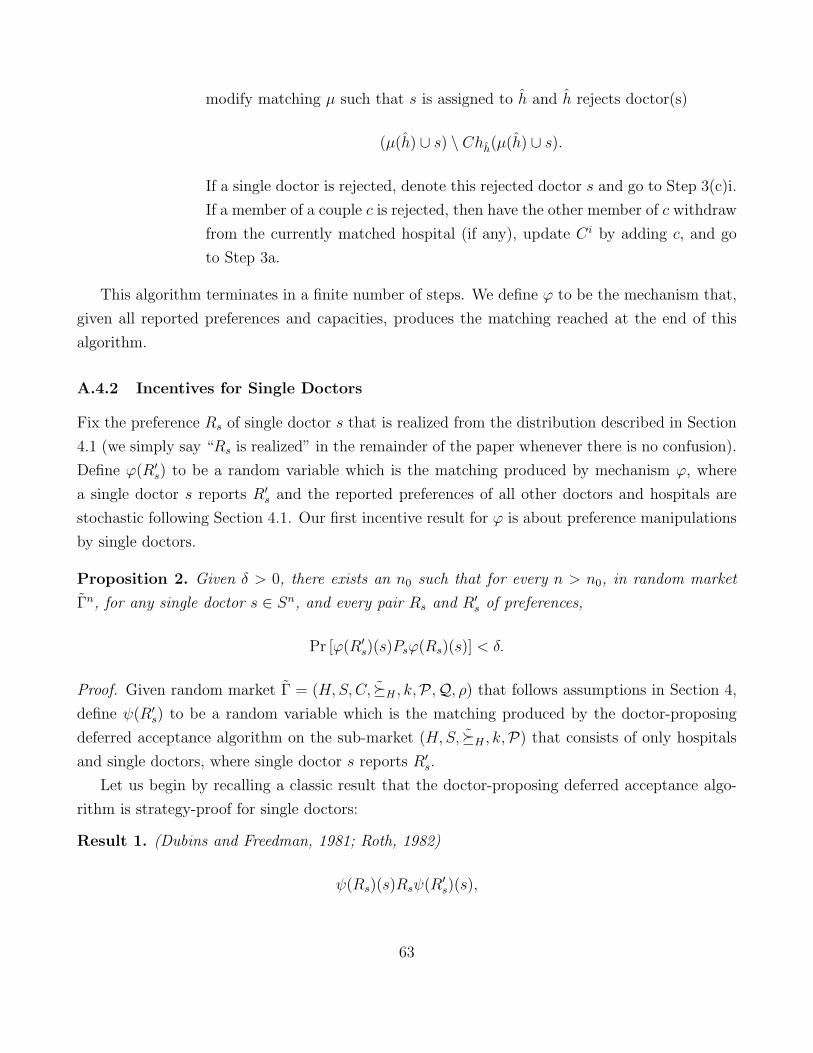
modify matching µ such that s is assigned to h and h rejects doctor(s)

(µ(h) ∪ s) \ Chh(µ(h) ∪ s).

If a single doctor is rejected, denote this rejected doctor s and go to Step 3(c)i.

If a member of a couple c is rejected, then have the other member of c withdraw

from the currently matched hospital (if any), update Ci by adding c, and go

to Step 3a.

This algorithm terminates in a finite number of steps. We define ϕ to be the mechanism that,

given all reported preferences and capacities, produces the matching reached at the end of this

algorithm.

A.4.2 Incentives for Single Doctors

Fix the preference Rs of single doctor s that is realized from the distribution described in Section

4.1 (we simply say “Rs is realized” in the remainder of the paper whenever there is no confusion).

Define ϕ(R′s) to be a random variable which is the matching produced by mechanism ϕ, where

a single doctor s reports R′s and the reported preferences of all other doctors and hospitals are

stochastic following Section 4.1. Our first incentive result for ϕ is about preference manipulations

by single doctors.

Proposition 2. Given δ > 0, there exists an n0 such that for every n > n0, in random market

Γn, for any single doctor s ∈ Sn, and every pair Rs and R′s of preferences,

Pr [ϕ(R′s)(s)Psϕ(Rs)(s)] < δ.

Proof. Given random market Γ = (H,S,C, �H , k,P ,Q, ρ) that follows assumptions in Section 4,

define ψ(R′s) to be a random variable which is the matching produced by the doctor-proposing

deferred acceptance algorithm on the sub-market (H,S, �H , k,P) that consists of only hospitals

and single doctors, where single doctor s reports R′s.

Let us begin by recalling a classic result that the doctor-proposing deferred acceptance algo-

rithm is strategy-proof for single doctors:

Result 1. (Dubins and Freedman, 1981; Roth, 1982)

ψ(Rs)(s)Rsψ(R′s)(s),

63

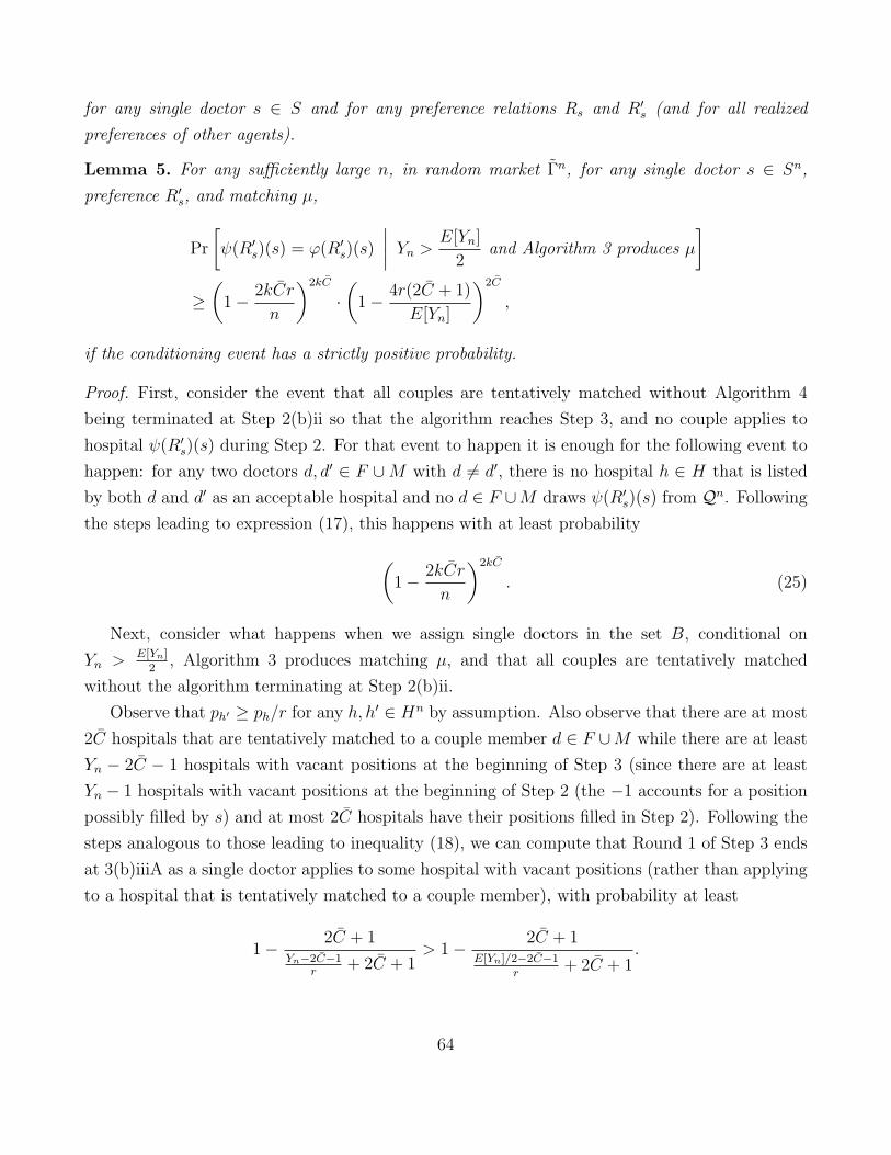
for any single doctor s ∈ S and for any preference relations Rs and R′s (and for all realized

preferences of other agents).

Lemma 5. For any sufficiently large n, in random market Γn, for any single doctor s ∈ Sn,

preference R′s, and matching µ,

Pr

[ψ(R′s)(s) = ϕ(R′s)(s)

∣∣∣∣ Yn > E[Yn]

2and Algorithm 3 produces µ

]≥(

1− 2kCr

n

)2kC

·(

1− 4r(2C + 1)

E[Yn]

)2C

,

if the conditioning event has a strictly positive probability.

Proof. First, consider the event that all couples are tentatively matched without Algorithm 4

being terminated at Step 2(b)ii so that the algorithm reaches Step 3, and no couple applies to

hospital ψ(R′s)(s) during Step 2. For that event to happen it is enough for the following event to

happen: for any two doctors d, d′ ∈ F ∪M with d 6= d′, there is no hospital h ∈ H that is listed

by both d and d′ as an acceptable hospital and no d ∈ F ∪M draws ψ(R′s)(s) from Qn. Following

the steps leading to expression (17), this happens with at least probability

(1− 2kCr

n

)2kC

. (25)

Next, consider what happens when we assign single doctors in the set B, conditional on

Yn > E[Yn]2

, Algorithm 3 produces matching µ, and that all couples are tentatively matched

without the algorithm terminating at Step 2(b)ii.

Observe that ph′ ≥ ph/r for any h, h′ ∈ Hn by assumption. Also observe that there are at most

2C hospitals that are tentatively matched to a couple member d ∈ F ∪M while there are at least

Yn − 2C − 1 hospitals with vacant positions at the beginning of Step 3 (since there are at least

Yn − 1 hospitals with vacant positions at the beginning of Step 2 (the −1 accounts for a position

possibly filled by s) and at most 2C hospitals have their positions filled in Step 2). Following the

steps analogous to those leading to inequality (18), we can compute that Round 1 of Step 3 ends

at 3(b)iiiA as a single doctor applies to some hospital with vacant positions (rather than applying

to a hospital that is tentatively matched to a couple member), with probability at least

1− 2C + 1Yn−2C−1

r+ 2C + 1

> 1− 2C + 1E[Yn]/2−2C−1

r+ 2C + 1

.

64

Now assume that all Rounds 1, . . . , j − 1 end at Step 3(b)iiiA. Then there are still at least

Yn − 2C − (j − 1)− 1 hospitals with a vacant position. This follows since at most j − 1 hospitals

have had their positions filled at Rounds 1, . . . , j − 1 among those hospitals that are not listed

on any single doctor’s preference list at the end of Algorithm 3. Following the steps analogous to

those leading to inequality (18), we can compute that Round j initiated by some single doctor in

Bj ends at Step 3(b)iiiA with probability of at least

1− 2C + 1E[Yn]/2−2C−(j−1)−1

r+ 2C + 1

.

Since there are at most 2C rounds (because this is the maximum number of single doctors who

could have been displaced by couples in Step 2), Algorithm 4 succeeds with conditional probability

of at least (1− 2C + 1

E[Yn]/4r

)2C

. (26)

Recall that the algorithm underlying ϕ coincides with the sequential couples algorithm if the

latter succeeds. This fact together with the arguments leading to expressions (25) and (26) imply

Pr

[ψ(R′s)(s) = ϕ(R′s)(s)

∣∣∣∣ Yn > E[Yn]

2and Algorithm 3 produces µ

]≥(

1− 2kCr

n

)2kC

·(

1− 4r(2C + 1)

E[Yn]

)2C

.

To prove Proposition 2 first note that, by Result 1 we have

Pr[ϕ(Rs)(s)Rsϕ(R′s)(s)] ≥ Pr [ψ(Rs)(s) = ϕ(Rs)(s) and ψ(R′s)(s) = ϕ(R′s)(s)] . (27)

By Lemma 5 we have

Pr

[ψ(R′s)(s) = ϕ(R′s)(s)

∣∣∣∣ Yn > E[Yn]

2and Algorithm 3 produces µ

]≥(

1− 2kCr

n

)2kC

·(

1− 4r(2C + 1)

E[Yn]

)2C

.

This inequality holds for any matching µ that is produced at the end of Algorithm 3. Therefore,

65

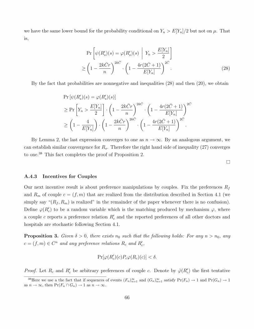
we have the same lower bound for the probability conditional on Yn > E[Yn]/2 but not on µ. That

is,

Pr

[ψ(R′s)(s) = ϕ(R′s)(s)

∣∣∣∣ Yn > E[Yn]

2

]≥(

1− 2kCr

n

)2kC

·(

1− 4r(2C + 1)

E[Yn]

)2C

. (28)

By the fact that probabilities are nonnegative and inequalities (28) and then (20), we obtain

Pr [ψ(R′s)(s) = ϕ(R′s)(s)]

≥ Pr

[Yn >

E[Yn]

2

]·(

1− 2kCr

n

)2kC

·(

1− 4r(2C + 1)

E[Yn]

)2C

≥(

1− 4

E[Yn]

)·(

1− 2kCr

n

)2kC

·(

1− 4r(2C + 1)

E[Yn]

)2C

.

By Lemma 2, the last expression converges to one as n→∞. By an analogous argument, we

can establish similar convergence for Rs. Therefore the right hand side of inequality (27) converges

to one.38 This fact completes the proof of Proposition 2.

A.4.3 Incentives for Couples

Our next incentive result is about preference manipulations by couples. Fix the preferences Rf

and Rm of couple c = (f,m) that are realized from the distribution described in Section 4.1 (we

simply say “(Rf , Rm) is realized” in the remainder of the paper whenever there is no confusion).

Define ϕ(R′c) to be a random variable which is the matching produced by mechanism ϕ, where

a couple c reports a preference relation R′c and the reported preferences of all other doctors and

hospitals are stochastic following Section 4.1.

Proposition 3. Given δ > 0, there exists n0 such that the following holds: For any n > n0, any

c = (f,m) ∈ Cn and any preference relations Rc and R′c,

Pr[ϕ(R′c)(c)Pcϕ(Rc)(c)] < δ.

Proof. Let Rc and R′c be arbitrary preferences of couple c. Denote by ϕ(R′c) the first tentative

38Here we use a the fact that if sequences of events (Fn)∞n=1 and (Gn)∞n=1 satisfy Pr(Fn) → 1 and Pr(Gn) → 1as n→∞, then Pr(Fn ∩Gn)→ 1 as n→∞.

66

assignments of couple c in Algorithm 5 under report R′c. Note that in that step, for any R′c,

couples receive their most preferred hospitals according to R′c among those that choose them if c

applies. As a result, ϕ(Rc)(c)Rcϕ(R′c)(c). Therefore, it suffices to demonstrate that

Pr [ϕ(Rc)(c) = ϕ(Rc)(c), ϕ(R′c)(c) = ϕ(R′c)(c)] > 1− δ.

We begin by proving a result similar to Lemma 5.

Lemma 6. For any sufficiently large n, R′c and µ,

Pr

[ϕ(R′c)(c) = ϕ(R′c)(c)

∣∣∣∣ Yn > E[Yn]

2and Algorithm 3 produces µ

]≥(

1− 2kCr

n

)2kC

·(

1− 8rC

E[Yn]

)2C

(29)

if the conditioning event has a strictly positive probability.

Proof. First, consider the event that all couples except for c are tentatively matched without

displacing members of any other couple. Following steps analogous to those leading to expression

(17), this happens with at least probability

(1− 2kCr

n

)2kC

. (30)

Next, we consider what happens when we assign single doctors in the set B, conditional on

Yn >E[Yn]

2and the event that all couples except for c are tentatively matched without displacing

members of any other couple. Following steps analogous to those leading up to inequality (19),

the set of single doctors in B do not displace any assigned couples with conditional probability of

at least (1− 2C

E[Yn]/4r

)2C

. (31)

By relations (30) and (31) and rearranging terms we obtain inequality (29), completing the proof.

To prove Proposition 3 recall that

Pr[ϕ(Rc)(c)Rcϕ(R′c)(c)] ≥ Pr [ϕ(Rc)(c) = ϕ(Rc)(c), ϕ(R′c)(c) = ϕ(R′c)(c)] . (32)

67

By Lemma 6 we have

Pr[ϕ(R′c)(c) = ϕ(R′c)(c) | Yn >

E[Yn]

2and Algorithm 3 produces µ

]≥(

1− 2kCr

n

)2kC

·(

1− 8rC

E[Yn]

)2C

.

This inequality holds for any matching µ that is produced at the end of Algorithm 3. Therefore,

we have the same lower bound for probability conditional on Yn > E[Yn]/2 but not on µ. That is,

Pr

[ϕ(R′c)(c) = ϕ(R′c)(c)

∣∣∣∣ Yn > E[Yn]

2

]≥(

1− 2kCr

n

)2kC

·(

1− 8rC

E[Yn]

)2C

. (33)

By the fact that probabilities are nonnegative and inequalities (33) and then (20), we obtain

Pr [ϕ(R′c)(c) = ϕ(R′c)(c)] ≥ Pr

[Yn >

E[Yn]

2

]·(

1− 2kCr

n

)2kC

·(

1− 4r(2C + 1)

E[Yn]

)2C

≥(

1− 4

E[Yn]

)·(

1− 2kCr

n

)2kC

·(

1− 4r(2C + 1)

E[Yn]

)2C

.

By Lemma 2, the last expression converges to one as n→∞. By an analogous argument, we

can establish similar convergence for Rc. Therefore the right hand side of inequality (32) converges

to one. This fact completes the proof of Proposition 3.

A.4.4 Incentives for Hospitals

Define ϕ(�′h) to be a random variable which is the matching produced by mechanism ϕ when a

hospital reports responsive preference �′h and the reported preferences of all other hospitals and

doctors are stochastic following Section 4.1.

Proposition 4. Given δ > 0, there exists an n0 such that for any n > n0, in random market Γn,

for all hospitals h ∈ Hn, for any pair of preferences �h and �′h,

Pr[ϕ(�′h)(h) �h ϕ(�h)(h)] < δ.

Proof. Define ψ(�′h) to be a random variable which is the matching produced by the doctor-

proposing deferred acceptance algorithm in which the only doctors in the market are single, and

hospital h reports �′h while the preferences of doctors are stochastic (and hence the matching is

a random variable).

68

Lemma 7. Given δ′ > 0, there exists an n0 such that for any n > n0, for all h ∈ Hn,�h and �′h,

Pr[ψ(�h)(h) �h ψ(�′h)(h)] > 1− δ′.

Proof. Lemma 10 of Kojima and Pathak (2009) implies this result.

Lemma 8. For any sufficiently large n, h ∈ Hn, �′h and µ,

Pr

[ψ(�′h)(h) = ϕ(�′h)(h)

∣∣∣∣ Yn > E[Yn]

2and Algorithm 3 produces µ

]≥(

1− 2kCr

n

)2kC

·(

1− 4r(2C + 1)

E[Yn]

)2C

if the conditioning event has a strictly positive probability.

Proof. The proof is analogous to the one for Lemma 5 where we replace ϕ(R′s)(s) with hospital h

throughout, so we omit it.

To complete the proof, observe that

Pr[ϕ(�h)(h) �h ϕ(�′h)(h)] ≥ Pr[ϕ(�h)(h) = ψ(�h)(h), ψ(�h)(h) �h ψ(�′h)(h), ψ(�′h)(h) = ϕ(�′h)(h)].

By Lemma 8 we have

Pr

[ψ(�′h)(h) = ϕ(�′h)(h)

∣∣∣∣∣ Yn > E[Yn]

2and Algorithm 3 produces µ

]

≥(

1− 2kCr

n

)2kC

·(

1− 4r(2C + 1)

E[Yn]

)2C

.

This inequality holds for any matching µ that is produced at the end of Algorithm 3. Therefore,

we have the same lower bound for the probability conditional on Yn > E[Yn]/2 but not on matching

µ. That is,

Pr

[ψ(�′h)(h) = ϕ(�′h)(h)

∣∣ Yn > E[Yn]

2

]≥(

1− 2kCr

n

)2kC

·(

1− 4r(2C + 1)

E[Yn]

)2C

. (34)

69

By the fact that probabilities are nonnegative and inequalities (34) and then (20), we obtain

Pr [ψ(�′h)(h) = ϕ(�′h)(h)] ≥ Pr

[Yn >

E[Yn]

2

]·(

1− 2kCr

n

)2kC

·(

1− 4r(2C + 1)

E[Yn]

)2C

≥(

1− 4

E[Yn]

)·(

1− 2kCr

n

)2kC

·(

1− 4r(2C + 1)

E[Yn]

)2C

.

By Lemma 2, the last expression converges to one as n → ∞. A similar convergence result

can be obtained for �h in lieu of �′h. These inequalities and Lemma 7 complete the proof of

Proposition 4.

A.4.5 Proof of Theorem 2

Fix ε > 0. By Propositions 2, 3 and 4, there exists n0 such that for any random market Γn

in the sequence with n > n0, any player, any of her true and misreported preferences, and any

other report of preferences, the probability that she is made better off by that misreporting of

preferences when every other player is reporting true preferences is less than

δ = ε

(max{ sup

n∈N,D′⊆Dn,h∈Hn,uh∈Uhuh(D

′), supn∈N,s∈Sn,h∈Hn,us∈Us

us(h), supn∈N,c∈Cn,h,h′∈Hn,uc∈Uc

uc(h, h′)})−1

,

where this bound is well-defined and positive by Condition (5) of Definition 2. This observation

immediately shows that

E[ui(ϕi(σi(ui), σ∗−i(u−i)))] ≤ E[ui(ϕi(σ

∗(u)))] + ε,

for any i, any type ui, and any strategy σi, completing the proof.

70

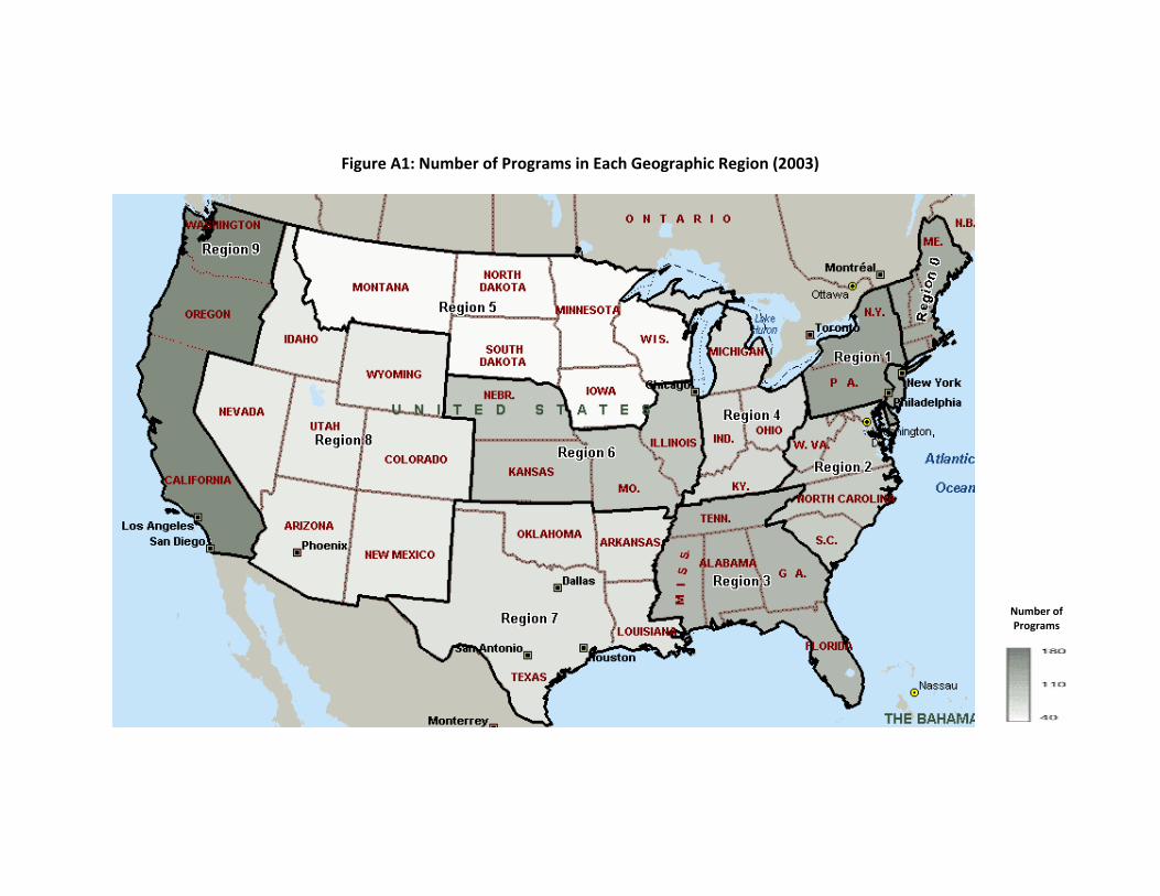
Figure A1: Number of Programs in Each Geographic Region (2003) 

        

Number of  Programs 

 

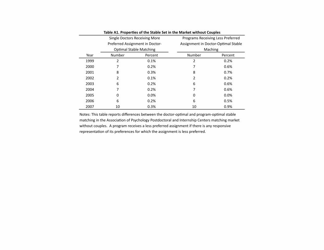
Year Number Percent Number Percent1999 2 0.1% 2 0.2%2000 7 0.2% 7 0.6%2001 8 0.3% 8 0.7%2002 2 0.1% 2 0.2%2003 6 0.2% 6 0.6%2004 7 0.2% 7 0.6%2005 0 0.0% 0 0.0%2006 6 0.2% 6 0.5%2007 10 0.3% 10 0.9%

SingleDoctorsReceivingMorePreferredAssignmentinDoctor‐

OpJmalStableMatching

ProgramsReceivingLessPreferredAssignmentinDoctor‐OpJmalStable

Maching

Notes:Thistablereportsdifferencesbetweenthedoctor‐opJmalandprogram‐opJmalstablematchingintheAssociaJonofPsychologyPostdoctoralandInternshipCentersmatchingmarketwithoutcouples.AprogramreceivesalesspreferredassignmentifthereisanyresponsiverepresentaJonofitspreferencesforwhichtheassignmentislesspreferred.

TableA1.Proper.esoftheStableSetintheMarketwithoutCouples