Munich Personal RePEc Archive

Matching with Couples: Stability and

Algorithm

Jiang, Zhishan and Tian, Guoqiang

Shanghai University of Finance and Economics, Texas AM

University

November 2013

Online at https://mpra.ub.uni-muenchen.de/57936/

MPRA Paper No. 57936, posted 18 Aug 2014 09:47 UTC

Matching with Couples: Stability and Algorithm

Zhishan Jiang

School of Economics

Shanghai University of Finance and Economics

Shanghai 200433, China

Guoqiang Tian∗

Department of Economics

Texas A&M University

College Station, TX 77843, USA

July, 2014

Abstract

This paper defines a notion of semi-stability for matching problem with couples, which is

a natural generalization of, and further identical to, the conventional stability for matching

without couples. It is shown that there always exists a semi-stable matching for couples

markets with strict preferences, and the set of semi-stable matchings can be partitioned in-

to subsets, each of which forms a distributive lattice. We further prove that a semi-stable

matching is stable when couples play reservation strategies. This result perfectly explains

the puzzle of NRMP even for finite markets. Moreover, we define a notion of asymptotic sta-

bility and present sufficient conditions for a sequential couples market to be asymptotically

stable. Another remarkable contribution is that we develop a new algorithm, called Persis-

tent Improvement Algorithm, for finding semi-stable matchings, which is also more efficient

than the Gale-Shapley algorithm for finding stable matchings for singles markets. Lastly,

this paper investigates the welfare property and incentive issues of semi-stable mechanisms.

Keywords: Matching with couples; stability; semi-stability; asymptotic stability; algo-

rithm.

JEL: C78, J41

∗Financial support from the National Natural Science Foundation of China (NSFC-71371117) and the Key

Laboratory of Mathematical Economics (SUFE) at Ministry of Education of China is gratefully acknowledged.

E-mail address: gtian@tamu.edu

1

1 Introduction

This paper studies the matching problem with couples. One typical feature of the problem

is that stable matchings may not exist in the presence of couples. To avoid this defect and find

sufficient conditions for the existence of stable matchings, we define the notion of semi-stability

as a generalized solution for matching problem with couples, which is a relaxation and natural

generalization of the conventional stability, and is further identical to the conventional stability

for matching without couples.

Matching is one of the most important natures of market. Many problems, such as trade

problem in consumption goods markets, employment problem in labor markets and auction

problem of indivisible/public goods, etc., can be regarded as matching problems. Gale and

Shapley (1962) were the first to introduce the notion of stable matching and regarded it as a

solution of matching problem. The deferred acceptance algorithm proposed by them reveals that

a stable matching always exists in one-to-one matching markets with strict preferences. Since

then, a lot of important theoretical results and their practice on matching have been developed

in key areas including education, health care, and army program such as the National Resident

Matching Program (NRMP) for medical students; student assignment mechanisms in major

school districts; kidney exchange programs; army programs, etc.

The NRMP has a long history. The original algorithm for NRMP proposed by Mullen and

Stalnaker (1952) was an unstable mechanism, and later, it was revised repeatedly as discussed in

detail in Roth and Peranson (1999). One of the reasons is that, since the 1970s, more and more

female medical students had entered the job market, which made NRMP’s algorithm run into

difficulties in finding stable outcomes. For instance, couples would often decline the job offers

assigned by the clearinghouse and search positions themselves in order to stay together, say, they

would prefer to have jobs in the same city, although the choice may not be the best for their

professional development. This implies that couple students’ preferences are complements. In

order to make the NRMP’s algorithm also work for couple medical students, Roth and Peranson

(1999) designed the NRMP’s present algorithm, but it may result in an empty set of stable

matchings since stable matching may not exist at all.

Sun and Yang (2006, 2009) studied the auction problem in economies where agents of the

same type are substitutes for one another, but agents of different types are complements. They

showed that equilibrium always exists in economies with quasi-linear preferences. Ostrovsky

(2008) studied a more generalized problem of supply chain networks in which there are similar

restrictions—same-side substitutability and cross-side complementarity, and showed that the

2

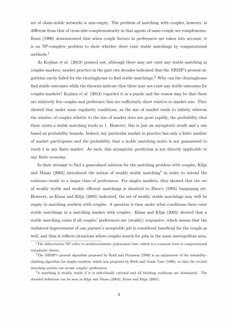
set of chain-stable networks is non-empty. The problem of matching with couples, however, is

different from that of cross-side complementarity in that agents of same-couple are complements.

Ronn (1990) demonstrated that when couple factors in preferences are taken into account, it

is an NP-complete problem to show whether there exist stable matchings by computational

methods.1

As Kojima et al. (2013) pointed out, although there may not exist any stable matching in

couples markets, market practice in the past two decades indicated that the NRMP’s present al-

gorithm rarely failed for the clearinghouse to find stable matchings.2 Why can the clearinghouse

find stable outcomes while the theories indicate that there may not exist any stable outcomes for

couples markets? Kojima et al. (2013) regarded it as a puzzle and the reason may be that there

are relatively few couples and preference lists are sufficiently short relative to market size. They

showed that under some regularity conditions, as the size of market tends to infinity whereas

the number of couples relative to the size of market does not grow rapidly, the probability that

there exists a stable matching tends to 1. However, this is just an asymptotic result and a one

based on probability bounds. Indeed, any particular market in practice has only a finite number

of market participants and the probability that a stable matching exists is not guaranteed to

reach 1 in any finite market. As such, this asymptotic prediction is not directly applicable to

any finite economy.

In their attempt to find a generalized solution for the matching problem with couples, Klijn

and Masso (2003) introduced the notion of weakly stable matching3 in order to extend the

existence result to a larger class of preferences. For singles markets, they showed that the set

of weakly stable and weakly efficient matchings is identical to Zhou’s (1994) bargaining set.

However, as Klaus and Klijn (2005) indicated, the set of weakly stable matchings may still be

empty in matching markets with couples. A question is then under what conditions there exist

stable matchings in a matching market with couples. Klaus and Klijn (2005) showed that a

stable matching exists if all couples’ preferences are (weakly) responsive, which means that the

unilateral improvement of one partner’s acceptable job is considered beneficial for the couple as

well, and thus it reflects situations where couples search for jobs in the same metropolitan area.

1The abbreviation NP refers to nondeterministic polynomial time, which is a common term in computational

complexity theory.2The NRMP’s present algorithm proposed by Roth and Peranson (1999) is an adjustment of the instability-

chaining algorithm for singles markets, which was proposed by Roth and Vande Vate (1990), so that the revised

matching system can accept couples’ preferences.3A matching is weakly stable if it is individually rational and all blocking coalitions are dominated. The

detailed definition can be seen in Klijn and Masso (2003), Klaus and Klijn (2005).

3

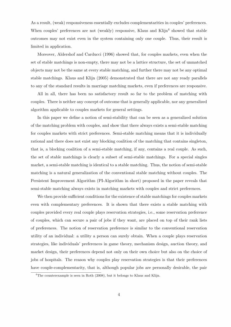
As a result, (weak) responsiveness essentially excludes complementarities in couples’ preferences.

When couples’ preferences are not (weakly) responsive, Klaus and Klijn4 showed that stable

outcomes may not exist even in the system containing only one couple. Thus, their result is

limited in application.

Moreover, Aldershof and Carducci (1996) showed that, for couples markets, even when the

set of stable matchings is non-empty, there may not be a lattice structure, the set of unmatched

objects may not be the same at every stable matching, and further there may not be any optimal

stable matchings. Klaus and Klijn (2005) demonstrated that there are not any ready parallels

to any of the standard results in marriage matching markets, even if preferences are responsive.

All in all, there has been no satisfactory result so far to the problem of matching with

couples. There is neither any concept of outcome that is generally applicable, nor any generalized

algorithm applicable to couples markets for general settings.

In this paper we define a notion of semi-stability that can be seen as a generalized solution

of the matching problem with couples, and show that there always exists a semi-stable matching

for couples markets with strict preferences. Semi-stable matching means that it is individually

rational and there does not exist any blocking coalition of the matching that contains singleton,

that is, a blocking coalition of a semi-stable matching, if any, contains a real couple. As such,

the set of stable matchings is clearly a subset of semi-stable matchings. For a special singles

market, a semi-stable matching is identical to a stable matching. Thus, the notion of semi-stable

matching is a natural generalization of the conventional stable matching without couples. The

Persistent Improvement Algorithm (PI-Algorithm in short) proposed in the paper reveals that

semi-stable matching always exists in matching markets with couples and strict preferences.

We then provide sufficient conditions for the existence of stable matchings for couples markets

even with complementary preferences. It is shown that there exists a stable matching with

couples provided every real couple plays reservation strategies, i.e., some reservation preference

of couples, which can secure a pair of jobs if they want, are placed on top of their rank lists

of preferences. The notion of reservation preference is similar to the conventional reservation

utility of an individual: a utility a person can surely obtain. When a couple plays reservation

strategies, like individuals’ preferences in game theory, mechanism design, auction theory, and

market design, their preferences depend not only on their own choice but also on the choice of

jobs of hospitals. The reason why couples play reservation strategies is that their preferences

have couple-complementarity, that is, although popular jobs are personally desirable, the pair

4The counterexample is seen in Roth (2008), but it belongs to Klaus and Klijn.

4

of popular jobs may not be the most preferred choice for couples, as they may not be at the

same hospital or in the same city. In order to stay together, the most preferred pair of jobs may

not be popular jobs, which is consistent with the practice of NRMP. As a consequence of the

sufficiency results, we provide a new explanation for the puzzle of NRMP raised in Kojima et

al. (2013). Moreover, these results perfectly explain the puzzle even for finite market because

they are not based on probability bounds and can be directly applicable to any finite economy.

This paper also defines a notion of asymptotic stability. In a large couples market, if the

number of couples is sufficiently small relative to that of singles, a semi-stable matching can

be deemed as an approaching stable matching. The number of blocking coalitions of any semi-

stable matching must be very small relative to the size of the market, if the length of rank list

of couples’ preferences does not quickly increase as the market goes very large. We define the

notion of the degree of unstable matching to indicate the unorderly degree of a matching. The

degree of instability is 0 for a stable matching, and 1 for the null matching in which all players

are unmatched. It is shown that under some simple regularity conditions, couples markets are

asymptotically stable, i.e., there exists a matching sequence whose instability degree sequence

tends to zero when the size of market tends to infinity. This conclusion is similar to the result

in Kojima et al. (2013), who demonstrated that the probability that a stable matching exists

converges to 1 as the market size approaches infinity under some regularity conditions. The

simple regularity conditions defined in this paper, however, are weaker than their regularity

conditions. As such, their result can be regarded as a special case of our result.

Another important contribution of the paper is to provide an algorithm called Persistent

Improvement Algorithm (PI-Algorithm in short) for finding a semi-stable matching, which is

also more efficient than the Gale-Shapley algorithm in the sense that it is quicker to find a

stable marching for singles markets. Crawford and Knoer (1981) and Kelso and Crawford

(1982) studied the employment problem in labor markets, and generalized the Gale-Shapley

algorithm by introducing the salary adjustment process. Hatfield and Milgrom (2005) extended

the Gale-Shapley algorithm into a generalized algorithm for matching with contracts, which

is in turn a generalization of the salary adjustment process of Kelso and Crawford (1982).

Ostrovsky (2008) studied a more generalized problem about supply chain networks in which

there are restrictions—same-side substitutability and cross-side complementarity, and presented

the T-Algorithm which generalizes the algorithms in Kelso and Crawford (1982), Hatfield and

Milgrom (2005), as well as the Gale-Shapley algorithm for marriage matching. However, the

problem of matching with couples is different from that of cross-side complementarity in that

5

agents of same-couple are complements. Those algorithms mentioned above cannot fit into the

couples markets. Roth and Vande Vate (1990) presented the instability-chaining algorithm for

one-to-one matching markets. The NRMP’s present algorithm proposed in Roth and Peranson

(1999) is an improvement of the instability-chaining algorithm for singles markets such that

the clearinghouse can accept the preferences of couples, but the algorithm may not converge.

This paper presents the PI-Algorithm which fits the couples markets. Moreover, it improves the

Gale-Shapley algorithm, through which we can find a stable matching quickly and which must

end in finite rounds for singles markets.

We also show that the set of semi-stable matchings can be partitioned into subsets, each of

which forms a distributive lattice, and in each of which there exist optimal semi-stable matchings

for couples side, truth-telling is a dominant strategy for hospitals side, and the set of unmatched

objects is the same at every semi-stable matching. We study welfare property and incentive

issues of semi-stable matching mechanisms from the perspective of market design, and generalize

respective results in marriage matching markets.

The remainder of this paper is organized as follows. Section II describes the setup and

introduces the notion of semi-stability in couples matchings. Section III provides the main results

on the existence of semi-stable matchings, stable matchings, asymptotically stable matching

sequence, and a generalized lattice theorem. We also provide a new explanation for the NRMP

puzzle. Section IV presents the PI-Algorithm and its properties. Section V discusses the welfare

and incentive properties of semi-stable matching mechanisms from the perspective of market

design. Section VI concludes and the appendix gives proofs of theorems.

2 A General Setting of Matching with Couples

To study matching with couples, without loss of generality, we restrict ourselves to a matching

market that consists of jobs of hospitals, job-seeking medical students and their preferences.

Although a hospital may provide many jobs, yet as Gale and Shapley (1962) and Roth and

Sotomayor (1990) pointed out, when medical students’ preferences are on specific jobs, it is

equivalent to the one-to-one marriage matching market. In fact, a hospital may provide some

jobs of special profession, such as physician jobs, surgeon jobs or gynecologist jobs, etc., and

the requirements for the jobs are generally different. As such, in this paper, matching objects

of medical students are jobs rather than hospitals.

Let H denote the set of jobs of hospitals, S the set of medical students and C the set of

student couples. Their elements are written as h, s, and c = (s, s′) respectively. For convenience

6

of discussion, we assume that null outcome is an element of sets H and S and a couple with

null partner is an element of C. To save notation, here we abuse ϕ to have denoted the null

elements/partner of sets H, S, and C. Specifically, null ϕ in H (resp. S) denotes the outside

option for doctors (resp. jobs), and c = (s, ϕ) in C denotes a special couple—single student. As

such, the model in this paper can actually be applied to two markets, i.e., the market containing

singles only, in short, singles market; the market containing couples (may containing singles or

not), in short, couples market.

We assume that all preferences of jobs and couples are strict. Let ≻h and ≻c denote h’s and

c’s preference relation, and P h and P c denote h’s and c’s preference list over students and pairs

of jobs, respectively. It is said that a student s ∈ S is acceptable (resp. unacceptable) to h if

s ≻h ϕ (resp. ϕ ≻h s), and (h, h′) ∈ H2 is acceptable (resp. unacceptable) pair of jobs to c if

(h, h′) ≻c (ϕ, ϕ) (resp. (ϕ, ϕ) ≻c (h, h′)). For convenience of discussion, we assume that ϕ and

(ϕ, ϕ) are at the last in P h and P c respectively. Let Γ = (H,S,C, (≻h)h∈H , (≻c)c∈C) denote a

couples market.

A matching µ is a one-to-one idempotent function from the set H ∪ S onto itself (i.e.,

µ2(x) = x for all x) such that µ(s) ∈ H and µ(h) ∈ S, where µ(s) and µ(h) are the matched

objects of s and h in µ. When a medical student or a job is not matched in µ, ϕ is regarded

as its matched object. For convenience, we assume µ(ϕ) = ϕ. Let µ(c) = (µ(s), µ(s′)) with

µ(s) ∈ H and µ(s′) ∈ H. For any µ, µ(s) = h if and only if µ(h) = s; µ(c) = (h, h′) if and only

if µ(h) = s and µ(h′) = s′.

If a job or a couple cannot be improved upon by voluntarily abandoning its matched object,

the matching is individually rational. Formally,

Definition 2.1 A matching µ is individually rational if (i) for all h ∈ H with µ(h) = ϕ,

µ(h) ≻h ϕ; and (ii) for all c = (s, s′) ∈ C, µ(c) ≻c (ϕ, µ(s′)) when µ(s) = ϕ, µ(c) ≻c (µ(s), ϕ)

when µ(s′) = ϕ, and µ(c) ≻c (ϕ, ϕ) when µ(c) = (ϕ, ϕ).

A couple and a pair of hospital jobs constitute a coalition. We then have the following

definitions.

Definition 2.2 {(s, s′), (h, h′)} ∈ C × H2 is called a blocking coalition of matching µ if (i)

(h, h′) ≻c µ(c); and (ii) [h = ϕ and µ(h) = s imply s ≻h µ(h)] and [h′ = ϕ and µ(h′) = s′ imply

s′ ≻h′ µ(h′)].

Thus, a blocking coalition means that agents can be improved upon by matching with each

other.

7

Definition 2.3 A matching is said to be stable if it is individually rational and there exist no

blocking coalitions.

Definition 2.4 A matching is said to be semi-stable if it is individually rational and there are

no blocking coalitions containing a single.

It is obvious that a stable matching is semi-stable, but the reverse in general is not true.

However, a semi-stable matching is a stable matching for any singles market. Indeed, when all

couples are (s, ϕ), it is identical to the definition of stable matching for singles markets. Thus,

the notion of semi-stability for couples markets is a natural generalization of the conventional

stability for singles markets. As Gale and Shapley (1962) showed, a stable matching always

exists for singles markets with strict preferences. However, for couples markets, Roth (1984)

showed that there may not exist any stable matching. In the next section, departing from Roth’s

example, we show that a semi-stable matching always exists for any couples market with strict

preferences and also provide sufficient conditions for the existence of stable matchings.

3 Main Existence Results and NRMP Puzzle Revisited

In this section, we first investigate the existence of semi-stable matching for couples markets

with strict preferences. We then show that the set of semi-stable matchings can be partitioned

into subsets, each of which forms a distributive lattice so that the couple-optimal matching exists

on each of partition sets. We also provide sufficient conditions for the existence of stability. The

results enable us to provide a new explanation for the puzzle of NRMP raised in Kojima et al.

(2013). Moreover, we define a notion of asymptotic stability and provide sufficient conditions

for a matching sequence to be asymptotically stable.

3.1 Existence of Semi-Stable Matching and Distributive Lattice

The example in Klaus and Klijn (2005) shows that, even if there is only one couple in a

matching market, there may not exist any stable matching. As such, if one focuses only on

stable matchings, the set of outcomes may be empty. This makes us introduce the notion

of semi-stable matching, which means that there does not exist any blocking coalition of the

matching that contains a single. A question is then whether there exists a semi-stable matching

for a couples market. The following theorem gives an affirmative answer.

Theorem 3.1 (Existence of Semi-Stable Matching) For any couples market Γ = (H,S,C,

(≻h)h∈H , (≻c)c∈C) with strict preferences, there exists a semi-stable matching µ.

8

The theorem indicates that a semi-stable matching always exists for strict preferences. Since

the theorem is proved by a constructive way, we actually obtain an algorithm to find a semi-

stable outcome. In addition, the algorithm also provides an approach to find a stable matching,

if any, in couples markets. Indeed, we first find a semi-stable matching, and then see if the

semi-stable matching is stable by verifying that there is no blocking coalition containing a real

couple. Of course, this is only a sufficient condition for stable matching, that is, if the semi-stable

matching is not stable, we cannot assert that there do not exist any stable matchings.

The Conway lattice theorem in the literature shows that the set of all stable matchings forms

a distributive lattice for a singles market with strict preferences so that there is a polarization

of interests between the two sides of the market along the set of stable matchings.5 This implies

that there exists a unique best stable matching µS favored by the students and a unique best

stable matching µH favored by the hospitals. Despite this nice property, Aldershof and Carducci

(1996) and Klaus and Klijin (2005) showed that, for couples markets, even when the set of stable

matchings is non-empty, there may be no optimal matching for either side of the market even

for the responsive preferences.

Can we have a similar result of this nice property for semi-stable matchings with couples?

The answer is affirmative in some sense. In any couples market with strict preferences, there

is a partition of the set of semi-stable matchings, each section of which forms a distributive

lattice. To show this, define two partial ordering relations ≥C and ≥H on matchings as follows.

For any two matchings µ1 and µ2, µ1 ≥C µ2 (resp. µ1 ≥H µ2) if and only if µ1(c) ≻c µ2(c)

or µ1(c) = µ2(c) (resp. µ1(h) ≻h µ2(h) or µ1(h) = µ2(h)) for every c ∈ C (resp. h ∈ H).

It is easily seen that both ≥C and ≥H are partial ordering relations, i.e., they are irreflexive,

anti-symmetric and transitive.

Consider a couples market Γ = (H,S,C, (≻h)h∈H , (≻c)c∈C). Let F be the set of all semi-

stable matchings, and µ1 and µ2 be two semi-stable matchings in F . We define two functions

∨C and ∧C that assign to each student his/her more preferred and less preferred match from µ1

and µ2, respectively. Formally, define two operators ∨C and ∧C as follows: for any c ∈ C

and µ1, µ2 ∈ F , let λ = µ1 ∨C µ2 and ν = µ1 ∧C µ2 where λ(c) = max≻c{µ1(c), µ2(c)},

ν(c) = min≻c{µ1(c), µ2(c)}. Similarly, we can define functions ∨H and ∧H . We then have

the following generalized lattice theorem.

Theorem 3.2 (Generalized Lattice Theorem) Let Γ = (H,S,C, (≻h)h∈H , (≻c)c∈C) be a

5The theorem is seen in Knuth (1976) and Roth and Sotomayor (1990), but it belongs to John Conway. A

lattice is a partially ordered set in which every two elements have a supremum and an infimum. A lattice is called

a distributive lattice if it also satisfies the law of distributivity.

9

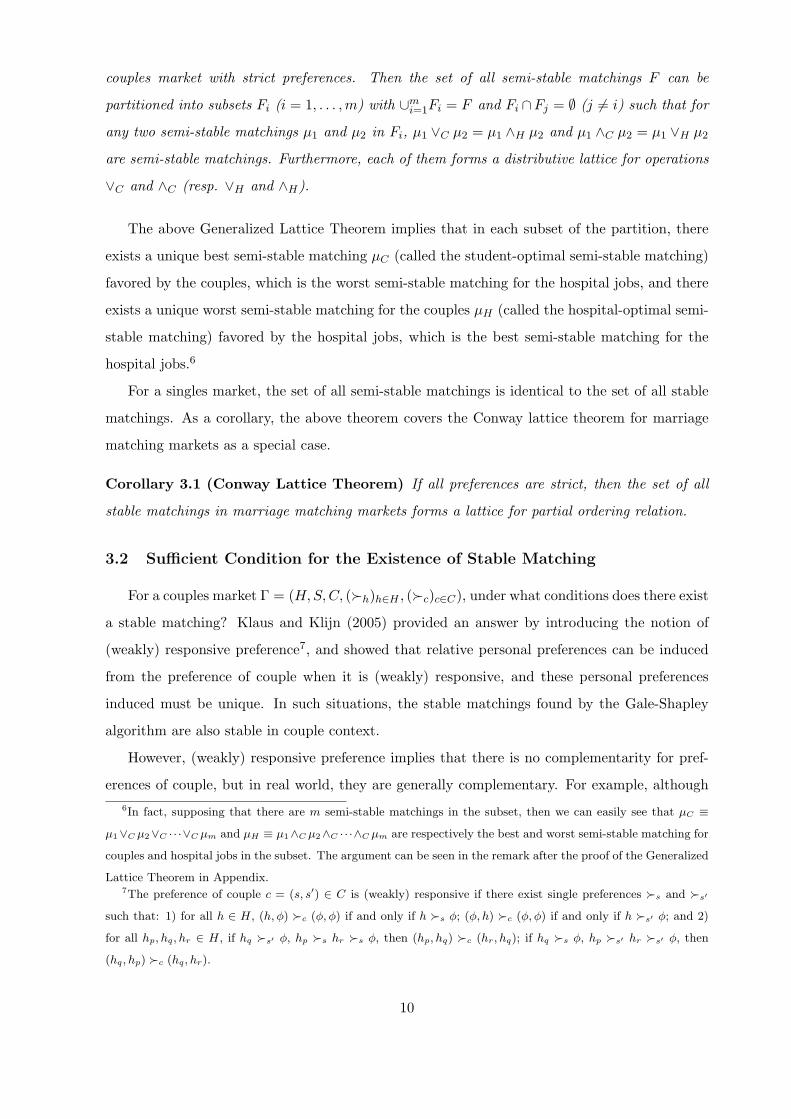
couples market with strict preferences. Then the set of all semi-stable matchings F can be

partitioned into subsets Fi (i = 1, . . . ,m) with ∪mi=1Fi = F and Fi ∩Fj = ∅ (j = i) such that for

any two semi-stable matchings µ1 and µ2 in Fi, µ1 ∨C µ2 = µ1 ∧H µ2 and µ1 ∧C µ2 = µ1 ∨H µ2

are semi-stable matchings. Furthermore, each of them forms a distributive lattice for operations

∨C and ∧C (resp. ∨H and ∧H).

The above Generalized Lattice Theorem implies that in each subset of the partition, there

exists a unique best semi-stable matching µC (called the student-optimal semi-stable matching)

favored by the couples, which is the worst semi-stable matching for the hospital jobs, and there

exists a unique worst semi-stable matching for the couples µH (called the hospital-optimal semi-

stable matching) favored by the hospital jobs, which is the best semi-stable matching for the

hospital jobs.6

For a singles market, the set of all semi-stable matchings is identical to the set of all stable

matchings. As a corollary, the above theorem covers the Conway lattice theorem for marriage

matching markets as a special case.

Corollary 3.1 (Conway Lattice Theorem) If all preferences are strict, then the set of all

stable matchings in marriage matching markets forms a lattice for partial ordering relation.

3.2 Sufficient Condition for the Existence of Stable Matching

For a couples market Γ = (H,S,C, (≻h)h∈H , (≻c)c∈C), under what conditions does there exist

a stable matching? Klaus and Klijn (2005) provided an answer by introducing the notion of

(weakly) responsive preference7, and showed that relative personal preferences can be induced

from the preference of couple when it is (weakly) responsive, and these personal preferences

induced must be unique. In such situations, the stable matchings found by the Gale-Shapley

algorithm are also stable in couple context.

However, (weakly) responsive preference implies that there is no complementarity for pref-

erences of couple, but in real world, they are generally complementary. For example, although

6In fact, supposing that there are m semi-stable matchings in the subset, then we can easily see that µC ≡

µ1∨C µ2∨C · · ·∨C µm and µH ≡ µ1∧C µ2∧C · · ·∧C µm are respectively the best and worst semi-stable matching for

couples and hospital jobs in the subset. The argument can be seen in the remark after the proof of the Generalized

Lattice Theorem in Appendix.7The preference of couple c = (s, s′) ∈ C is (weakly) responsive if there exist single preferences ≻s and ≻s′

such that: 1) for all h ∈ H, (h, φ) ≻c (φ, φ) if and only if h ≻s φ; (φ, h) ≻c (φ, φ) if and only if h ≻s′ φ; and 2)

for all hp, hq, hr ∈ H, if hq ≻s′ φ, hp ≻s hr ≻s φ, then (hp, hq) ≻c (hr, hq); if hq ≻s φ, hp ≻s′ hr ≻s′ φ, then

(hq, hp) ≻c (hq, hr).

10

for an individual s, hp ≻s hr, yet for couple c = (s, s′) ∈ C, (hr,hq) ≻c (hp, hq), as hq and hr

are in Boston whereas hp is in New York. Thus, the preference of the couple c is not (weakly)

responsive. If so, there may not exist any stable outcomes even in markets containing only one

couple.

In this subsection, we provide a sufficient condition for the existence of stable matching

even in the presence of complementary preferences of couples. To do so, we first introduce the

following notion.

Definition 3.1 (Reservation Preference) A pair of jobs (h, h′) ∈ H2 is said to be a reser-

vation preference job pair of a couple c = (s, s′) ∈ C if (i) (h, h′) ≻c (ϕ, ϕ), (ii) whenever h = ϕ,

s ≻h s for all s ∈ P h\{s}, and (iii) whenever h′ = ϕ, s′ ≻h′ s′ for all s′ ∈ P h′

\{s′}.

A reservation preference of a couple means that the couple can get a pair of jobs if they

want, as the members of the couple are respectively the most preferred medical students for the

relevant jobs of hospitals. It may be remarked that, when a couple plays reservation strategies,

like individuals’ preferences in game theory, mechanism design, auction theory, and market

design, their preferences depend not only on their own choice but also on the choice of jobs of

hospitals. The notion of reservation preference is also similar to the conventional reservation

utility of an individual. While reservation utility is a utility that a person can surely obtain by

outside opportunities and in turn may depend on preferences of other individuals, reservation

preference means that the couple can surely get the jobs since the couple is most preferred

students to the jobs.

We then have the following theorem which shows that there must exist a stable matching if

the first preference of each couple is one of its reservation preferences.

Theorem 3.3 (Sufficient Condition I for the Existence of Stable Matching) Let Γ =

(H,S,C, (≻h)h∈H , (≻c)c∈C) be a couples market with strict preferences. Suppose that for all

c ∈ C with s, s′ = ϕ, the first preference job pair (h, h′) in P c is a reservation preference job

pair of c. Then, there exists a stable matching µ.

The reason why a reservation preference job pair may be the first priority of a real couple

is that its preferences have couple-complementarity, that is, although one wants some popular

jobs, the pair of popular jobs may not be the most preferred choice for couples. Since the pair

of popular jobs may not be at the same hospital or in the same city, the most preferred job

pair for a couple may not be popular jobs, but may be its reservation preference job pair. In

11

the later subsection, we will give a generalized version of the theorem with more slack condition

that reservation preference job pair of real couples may not be their first preference job pair.

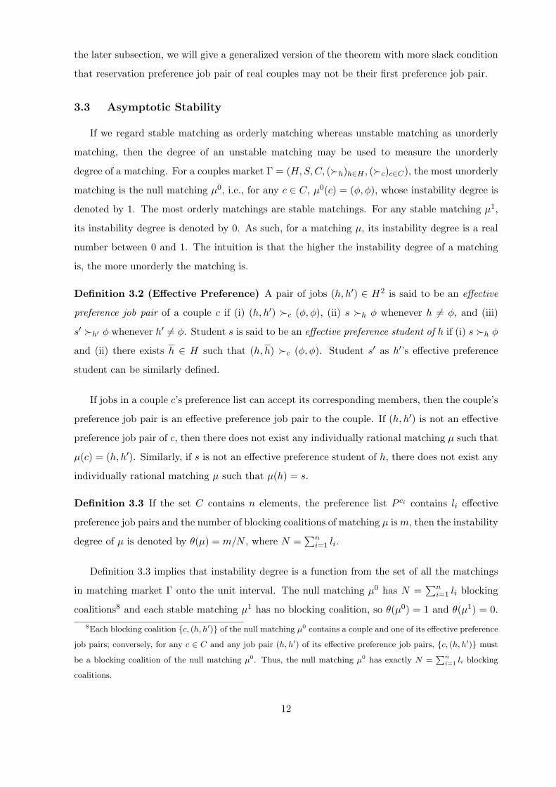
3.3 Asymptotic Stability

If we regard stable matching as orderly matching whereas unstable matching as unorderly

matching, then the degree of an unstable matching may be used to measure the unorderly

degree of a matching. For a couples market Γ = (H,S,C, (≻h)h∈H , (≻c)c∈C), the most unorderly

matching is the null matching µ0, i.e., for any c ∈ C, µ0(c) = (ϕ, ϕ), whose instability degree is

denoted by 1. The most orderly matchings are stable matchings. For any stable matching µ1,

its instability degree is denoted by 0. As such, for a matching µ, its instability degree is a real

number between 0 and 1. The intuition is that the higher the instability degree of a matching

is, the more unorderly the matching is.

Definition 3.2 (Effective Preference) A pair of jobs (h, h′) ∈ H2 is said to be an effective

preference job pair of a couple c if (i) (h, h′) ≻c (ϕ, ϕ), (ii) s ≻h ϕ whenever h = ϕ, and (iii)

s′ ≻h′ ϕ whenever h′ = ϕ. Student s is said to be an effective preference student of h if (i) s ≻h ϕ

and (ii) there exists h ∈ H such that (h, h) ≻c (ϕ, ϕ). Student s′ as h′’s effective preference

student can be similarly defined.

If jobs in a couple c’s preference list can accept its corresponding members, then the couple’s

preference job pair is an effective preference job pair to the couple. If (h, h′) is not an effective

preference job pair of c, then there does not exist any individually rational matching µ such that

µ(c) = (h, h′). Similarly, if s is not an effective preference student of h, there does not exist any

individually rational matching µ such that µ(h) = s.

Definition 3.3 If the set C contains n elements, the preference list P ci contains li effective

preference job pairs and the number of blocking coalitions of matching µ ism, then the instability

degree of µ is denoted by θ(µ) = m/N , where N =∑n

i=1li.

Definition 3.3 implies that instability degree is a function from the set of all the matchings

in matching market Γ onto the unit interval. The null matching µ0 has N =∑n

i=1li blocking

coalitions8 and each stable matching µ1 has no blocking coalition, so θ(µ0) = 1 and θ(µ1) = 0.

8Each blocking coalition {c, (h, h′)} of the null matching µ0 contains a couple and one of its effective preference

job pairs; conversely, for any c ∈ C and any job pair (h, h′) of its effective preference job pairs, {c, (h, h′)} must

be a blocking coalition of the null matching µ0. Thus, the null matching µ0 has exactly N =∑n

i=1li blocking

coalitions.

12

Thus, for any matching µ, if it has m blocking coalitions, obviously 0 ≤ m ≤ N , and thus the

degree of instability θ(µ) ∈ [0, 1]. Intuitively, the more blocking coalitions a matching has, the

more unorderly it is. Thus, the lower the instability degree of a matching is, the more orderly

and stable it is.

Definition 3.4 Let {Γk}∞k=1be a sequence of couples markets with Γk = (Hk, Sk, Ck, (≻h

)h∈Hk , (≻c)c∈Ck), and let µk be a matching of Γk, k = 1, 2, · · · . The matching sequence {µk}∞k=1

is said to be asymptotically stable if limk→∞{θ(µk)}∞k=1= 0. {Γk}∞k=1

is said to be asymptotically

stable if there exists a matching sequence {µk}∞k=1that is asymptotically stable.

Based on some common features of large matching markets in reality, Kojima and Pathak

(2009) first presented the notion of regular markets. Kojima et al. (2013) then defined the regular

markets for couples matchings, and demonstrated that for a regular sequence of couples markets,

the probability that a stable matching exists converges to 1 as the market size approaches infinity

whereas the number of couples relative to the market size does not grow rapidly.

Here we define the notion of simple regular couples markets. Consider a sequence of markets

of different sizes. For a sequence of couples markets, {Γk}∞k=1with Γk = (Hk, Sk, Ck, (≻h

)h∈Hk , (≻c)c∈Ck), there are∣∣Ck

∣∣ = nk, mk real couples, and lc effective preference job pairs in

P c.

Definition 3.5 A sequence of markets {Γk}∞k=1is said to be simple regular if it satisfies the

following conditions:

(1) mk ≤ nk1−ϵ for all k and a small positive ϵ;

(2) For any c ∈ C with s′ = ϕ, lc ≤ γ(lnnk)λ, where γ and λ are constants;

(3) (Participation Constraint) For any c ∈ C, lc > 0.

Condition (1) implies the fact that the number of real couples is small relative to the number

of singles. Condition (2) requires that the number of effective preference job pairs of real couples

be very small relative to the number of possible pairs of jobs. Condition (3) is actually a

participation constraint. For any couple c, if lc = 0, then for any individually rational matching

µ, µ(c) = (ϕ, ϕ), so it will not participate in the matching market. We then have the following

theorem.

Theorem 3.4 (Asymptotic Stability) Suppose that {Γk}∞k=1is a sequence of simple regular

couples markets with strict preferences where Γk = (Hk, Sk, Ck, (≻h)h∈Hk , (≻c)c∈Ck). Then

13

there exists a matching sequence {µk}∞k=1that is asymptotically stable when nk tends to infinity,

that is, {Γk}∞k=1is asymptotically stable.

The theorem indicates that there almost always exists a stable matching when the size of

a simple regular market tends to infinity. As the simple regularity conditions are weaker than

the regularity conditions proposed in Kojima et al. (2013), their result that the probability of

the existence of a stable matching converges to 1 as the market size approaches infinity can be

regarded as a special case of the above asymptotic stability theorem.

3.4 NRMP Puzzle Revisited

In the past two decades, NRMP’s practice has shown that the clearinghouse seldom fails to

find a stable matching. Kojima et al. (2013) pointed out that it is a puzzle. In fact, the reason

is that the NRMP market has many special features, which are described as eight stylized facts

by them. Here are the first four stylized facts.

Fact 1: Applicants who participate as couples constitute a small fraction of all participating

applicants.

Fact 2: The length of the rank order lists of applicants who are single or couples is small

relative to the number of possible programs.

Fact 3: The most popular programs are ranked as a top choice by a small number of appli-

cants.

Fact 4: A pair of internship programs ranked by doctors who participate as a couple tend

to be in the same region.

Kojima et al. (2013) pointed out that, in the data of NRMP during 1992-2009, applicants

who participated as couples are on average 4.4% of all applicants, the length of single applicants’

preference lists is on average about 7-9 programs, which is about 0.3% of the number of all

possible programs, and the length of couple applicants’ rank lists is about 81 on average, which

is less than 3% of the number of all possible programs. Thus, both are small relative to the

number of possible programs.

Since a matching of which the instability degree is zero must be stable, the asymptotic

stability theorem indicates that there almost always exists a stable matching when the size of

simple regular markets approaches infinity. Facts 1 and 2 imply that the NRMP’s practice

satisfies the simple regularity conditions, so the asymptotic stability theorem, Theorem 3.4, is

a good interpretation for the puzzle of NRMP.

Considering the stylized Fact 3 of NRMP market, most of popular jobs are placed at the top

14

of their preference rank lists by only a small number of medical students. This indicates that

the first preference jobs of most students are not their most preferred choices. Why is this true?

It is because couple are complementary, and they want to stay in the same location. As such,

the pair of popular jobs may not be the most preferred choice for couples as they may not be at

the same hospital or in the same city. Fact 4 exactly describes this, which indicates that a pair

of internship programs ranked by doctors who participate as a couple tend to be in the same

region. Combining Facts 3 and 4, one can assess that real couples have more incentives to play

reservation strategies than singles, i.e., they place one of their reservation preference job pairs,

rather than popular jobs, at the top of their rank order list (ROL) of preferences. As a result,

by Theorem 3.3, there exists a stable matching. Thus, this theoretical result explains why the

clearinghouse seldom fails to find a stable matching in NRMP’s practice even if the market may

not be large.

Table 1: Summary Statistics of Psychology Labor Market

TotalMean length for

rank order list (ROL)

Geographic similarity

for preference

Single doctors 3010 7.6

♯ Regions ranked 2.5

Couples 19 81.2

♯ Regions ranked 3.9

Fraction of ROL where

members rank same region73.4%

Notes: The data are from Kojima et al. (2013). This table reports descriptive information

from the Association of Psychology Postdoctoral and Internship Centers match, averaged over

1999-2007. Single doctors’ rank order lists consist of a ranking over hospital jobs, while couples’

indicate rankings over pairs of hospital jobs.

From the statistical data in Tables 1 and 2, we can see these facts are true. Table 1 indicates

that the fraction of rank order list where both members rank the same region, i.e., the preference

having couple-complementarity, is 73.4%, which coincides with Fact 4. It shows that the pair

of jobs having couple-complementarity surely provides the couple with extra welfare, so it gives

couples more incentives than singles to play reservation strategies. Real couples play reservation

strategies, which coincides with Fact 3 that the most popular programs are ranked as a top

choice by a small number of applicants. This actually shows that not only most real couples but

15

also most singles play reservation strategies.

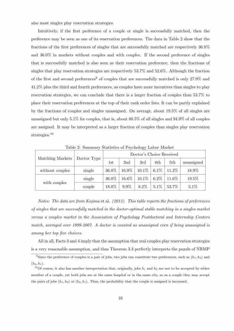
Intuitively, if the first preference of a couple or single is successfully matched, then the

preference may be seen as one of its reservation preferences. The data in Table 2 show that the

fractions of the first preferences of singles that are successfully matched are respectively 36.8%

and 36.0% in markets without couples and with couples. If the second preference of singles

that is successfully matched is also seen as their reservation preference, then the fractions of

singles that play reservation strategies are respectively 53.7% and 52.6%. Although the fraction

of the first and second preferences9 of couples that are successfully matched is only 27.9% and

41.2% plus the third and fourth preferences, as couples have more incentives than singles to play

reservation strategies, we can conclude that there is a larger fraction of couples than 53.7% to

place their reservation preferences at the top of their rank order lists. It can be partly explained

by the fractions of couples and singles unassigned. On average, about 19.5% of all singles are

unassigned but only 5.1% for couples, that is, about 80.5% of all singles and 94.9% of all couples

are assigned. It may be interpreted as a larger fraction of couples than singles play reservation

strategies.10

Table 2: Summary Statistics of Psychology Labor Market

Matching Markets Doctor TypeDoctor’s Choice Received

1st 2nd 3rd 4th 5th unassigned

without couples single 36.8% 16.9% 10.1% 6.1% 11.2% 18.9%

with couplessingle 36.0% 16.6% 10.1% 6.2% 11.6% 19.5%

couple 18.0% 9.9% 8.2% 5.1% 53.7% 5.1%

Notes: The data are from Kojima et al. (2013). This table reports the fractions of preferences

of singles that are successfully matched in the doctor-optimal stable matching in a singles market

versus a couples market in the Association of Psychology Postdoctoral and Internship Centers

match, averaged over 1999-2007. A doctor is counted as unassigned even if being unassigned is

among her top five choices.

All in all, Facts 3 and 4 imply that the assumption that real couples play reservation strategies

is a very reasonable assumption, and thus Theorem 3.3 perfectly interprets the puzzle of NRMP

9Since the preference of couples is a pair of jobs, two jobs can constitute two preferences, such as (h1, h2) and

(h2, h1).10Of course, it also has another interpretation that, originally, jobs h1 and h2 are not to be accepted by either

member of a couple, yet both jobs are at the same hospital or in the same city, so as a couple they may accept

the pairs of jobs (h1, h2) or (h2, h1). Thus, the probability that the couple is assigned is increased.

16

because we need not impose the unrealistic assumption that market goes to infinity and it is

not based on probability bounds. Theorem 3.3 holds even for finite market. In contrast, the

result of Kojima et al. (2013) is an asymptotic result that is based on probability bounds.

The probability that a stable matching exists is not guaranteed to reach 1 in any finite market.

Since any particular market in practice has only a finite number of market participants, their

asymptotic prediction is not directly applicable to any finite economy.

In fact, the condition of Theorem 3.3 can be further weakened. Provided the preferences in

front of real couples’ first reservation preferences are not pairs of popular jobs, then there exists

a stable matching. Since the number of couples is very small relative to the number of singles,

we may consider that all popular jobs are assigned to singles. The data in Table 1 show that the

number of singles is 3010 whereas the number of couples is 19, and the fraction of singles whose

first preferences are successfully assigned is over 36% (which means more than 1000 jobs, and

we may consider that almost all popular jobs are among the 1000 jobs). The following theorem

shows that there exists a stable matching in such markets, which is another strong interpretation

for the puzzle of NRMP.

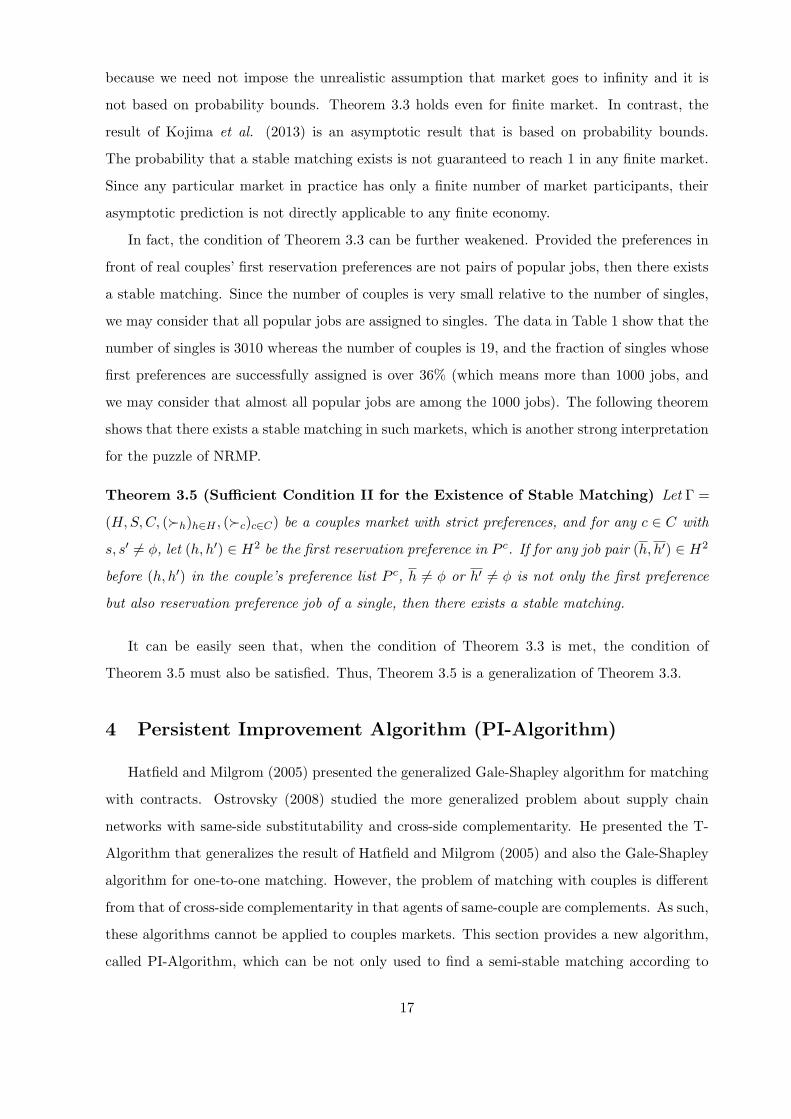
Theorem 3.5 (Sufficient Condition II for the Existence of Stable Matching) Let Γ =

(H,S,C, (≻h)h∈H , (≻c)c∈C) be a couples market with strict preferences, and for any c ∈ C with

s, s′ = ϕ, let (h, h′) ∈ H2 be the first reservation preference in P c. If for any job pair (h, h′) ∈ H2

before (h, h′) in the couple’s preference list P c, h = ϕ or h′ = ϕ is not only the first preference

but also reservation preference job of a single, then there exists a stable matching.

It can be easily seen that, when the condition of Theorem 3.3 is met, the condition of

Theorem 3.5 must also be satisfied. Thus, Theorem 3.5 is a generalization of Theorem 3.3.

4 Persistent Improvement Algorithm (PI-Algorithm)

Hatfield and Milgrom (2005) presented the generalized Gale-Shapley algorithm for matching

with contracts. Ostrovsky (2008) studied the more generalized problem about supply chain

networks with same-side substitutability and cross-side complementarity. He presented the T-

Algorithm that generalizes the result of Hatfield and Milgrom (2005) and also the Gale-Shapley

algorithm for one-to-one matching. However, the problem of matching with couples is different

from that of cross-side complementarity in that agents of same-couple are complements. As such,

these algorithms cannot be applied to couples markets. This section provides a new algorithm,

called PI-Algorithm, which can be not only used to find a semi-stable matching according to

17

the steps described in the proof of Theorem 3.1, but also more efficient than the Gale-Shapley

algorithm for finding stable matchings in singles markets.

4.1 The PI-Algorithm

Given a couples market Γ = (H,S,C, (≻h)h∈H , (≻c)c∈C), let P h and P c be h’s and c’s

preference list. Similar to Hatfield and Milgrom (2005), we denote the space of contract X =

(S ×H) ∪ {Φ} and the space of contract pairs Z = X ×X, where Φ denotes null contract. For

convenience, we say that (s, ϕ) and (ϕ, h) are both null contracts. A contract x = (s, h) ∈ X

denotes a matching pair between a medical student s and a hospital job h, and a medical student

can sign only a contract with any given job. If a medical student (resp. a hospital job) does

not sign any contract with any hospital job (resp. any medical student), we say it signs a null

contract Φ. That is, in any case, a medical student (resp. a hospital job) can sign a null contract

if he/she (resp. it) does not want to sign a contract with any hospital job (resp. any medical

student). A contract pair z = ((s, h), (s′, h′)) ∈ Z denotes a group of matchings between a couple

c = (s, s′) and a pair of jobs (h, h′). The running steps of the PI-Algorithm are a sequential

process in which contracts are chosen by hospital jobs and couples.

Given that a set of contracts X ′ j X, a job h and a couple c will make their optimal

choices by their preference lists. Let Chh : 2X → X and Chc : 2X → Z denote their best-

response mappings so that every subset X ′ of X corresponds to Chh(X′) and Chc(X

′), which

are respectively a contract and a contract pair. If there is no better choice than vacancy for

h, h’s choice is a null contract; otherwise, it is a contract between h and its most preferred

student. For couples’ choices, it is a little more complicated. The couple c chooses an optimal

contract pair by its preference list which may contain two null contracts, a null contract or no

null contract. Formally, the best-response mappings Chh(·) and Chc(·) of hospital jobs and

couples are defined as follows:

Chh(X′) =

Φ if Ah = ∅

(s, h) otherwise,

where Ah = {s : s ≻h ϕ and (s, h) ∈ X ′} is the set of students acceptable to the job h and ∅

denotes the empty set, and s = max ≻h {s : (s, h) ∈ X ′} is the maximal element in Ah.

For c = (s, s′), the best-response mapping Chc(·) of couples is given by

Chc(X′) =

(Φ,Φ) if Ac = ∅

((s, h), (s′, h′)) otherwise,

18

where Ac = {(h, h′) : (h, h′) ≻c (ϕ, ϕ) and ((s, h), (s′, h′)) ∈ X ′ × X ′} is the set of job pairs

acceptable to the couple c, and (h, h′) = max ≻c {(h, h′) : ((s, h), (s′, h′)) ∈ X ′ × X ′} is the

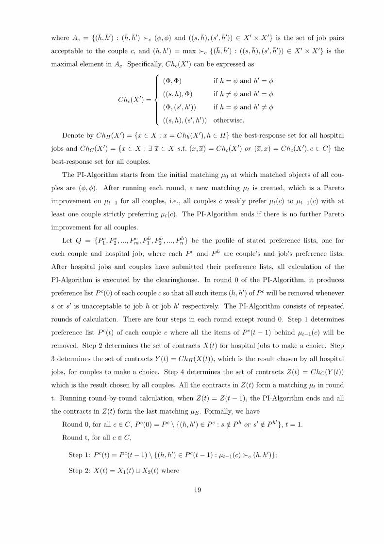
maximal element in Ac. Specifically, Chc(X′) can be expressed as

Chc(X′) =

(Φ,Φ) if h = ϕ and h′ = ϕ

((s, h),Φ) if h = ϕ and h′ = ϕ

(Φ, (s′, h′)) if h = ϕ and h′ = ϕ

((s, h), (s′, h′)) otherwise.

Denote by ChH(X ′) = {x ∈ X : x = Chh(X′), h ∈ H} the best-response set for all hospital

jobs and ChC(X′) = {x ∈ X : ∃ x ∈ X s.t. (x, x) = Chc(X

′) or (x, x) = Chc(X′), c ∈ C} the

best-response set for all couples.

The PI-Algorithm starts from the initial matching µ0 at which matched objects of all cou-

ples are (ϕ, ϕ). After running each round, a new matching µt is created, which is a Pareto

improvement on µt−1 for all couples, i.e., all couples c weakly prefer µt(c) to µt−1(c) with at

least one couple strictly preferring µt(c). The PI-Algorithm ends if there is no further Pareto

improvement for all couples.

Let Q = {P c1 , P

c2 , ..., P

cm, P h

1 , Ph2 , ..., P

hn } be the profile of stated preference lists, one for

each couple and hospital job, where each P c and P h are couple’s and job’s preference lists.

After hospital jobs and couples have submitted their preference lists, all calculation of the

PI-Algorithm is executed by the clearinghouse. In round 0 of the PI-Algorithm, it produces

preference list P c(0) of each couple c so that all such items (h, h′) of P c will be removed whenever

s or s′ is unacceptable to job h or job h′ respectively. The PI-Algorithm consists of repeated

rounds of calculation. There are four steps in each round except round 0. Step 1 determines

preference list P c(t) of each couple c where all the items of P c(t − 1) behind µt−1(c) will be

removed. Step 2 determines the set of contracts X(t) for hospital jobs to make a choice. Step

3 determines the set of contracts Y (t) = ChH(X(t)), which is the result chosen by all hospital

jobs, for couples to make a choice. Step 4 determines the set of contracts Z(t) = ChC(Y (t))

which is the result chosen by all couples. All the contracts in Z(t) form a matching µt in round

t. Running round-by-round calculation, when Z(t) = Z(t − 1), the PI-Algorithm ends and all

the contracts in Z(t) form the last matching µE . Formally, we have

Round 0, for all c ∈ C, P c(0) = P c \ {(h, h′) ∈ P c : s /∈ P h or s′ /∈ P h′

}, t = 1.

Round t, for all c ∈ C,

Step 1: P c(t) = P c(t− 1) \ {(h, h′) ∈ P c(t− 1) : µt−1(c) ≻c (h, h′)};

Step 2: X(t) = X1(t) ∪X2(t) where

19

X1(t) = ∪c∈C{(s, h) ∈ X : there exists h′ ∈ H such that (h, h′) ∈ P c(t) \ {(ϕ, ϕ)}},

X2(t) = ∪c∈C{(s′, h′) ∈ X : there exists h ∈ H such that (h, h′) ∈ P c(t) \ {(ϕ, ϕ)}};

Step 3: Y (t) = ChH(X(t));

Step 4: Z(t) = ChC(Y (t)), we obtain the matching µt. If Z(t) = Z(t− 1), then the

PI-Algorithm ends; else t = t+ 1 and it goes to Round t.

We will illustrate these steps of the PI-Algorithm by the following example.

4.2 The PI-Algorithm: An Example

Example 4.1 c1 = (s1, s2) and c2 = (s3, s4) are couples, c3 = (s5, ϕ) and c4 = (s6, ϕ) are

singles. There are five hospital jobs h1, h2, h3, h4 and h5. Their preference lists are as follows:

c1 : {(h1, h2), (h3, h4), (h1, ϕ), (h3, ϕ), (ϕ, h2), (ϕ, h4), (ϕ, ϕ)};

c2 : {(h1, h2), (h3, h5), (h1, ϕ), (h3, ϕ), (ϕ, h2), (ϕ, h5), (ϕ, ϕ)};

c3 : {(h1, ϕ), (h2, ϕ), (h3, ϕ), (h5, ϕ), (ϕ, ϕ)};

c4 : {(h1, ϕ), (h2, ϕ), (h3, ϕ), (h4, ϕ), (ϕ, ϕ)};

h1 : {s1, s3, s5, ϕ}; h2 : {s2, s4, s6, ϕ}; h3 : {s1, s3, s5, ϕ};

h4 : {s2, s4, s6, ϕ}; h5 : {s2, s4, s5, ϕ}.

The running procedures of the PI-Algorithm for the example are specified as in Table 3. In

round 0, it removes all the items of preference lists of all couples that are not acceptable to

hospital jobs. After round 1 and round 2, it has actually produced the last matching. Round 3

repeats round 2 and thus the PI-Algorithm ends. We obtain the following matching.

µE(c1) = (h1, h2), µE(c2) = (h3, h5), µE(c3) = (ϕ, ϕ), µE(c4) = (h4, ϕ).

We can easily verify the matching obtained is stable. The matched object of c1 is the most

preferred choice and therefore there does not exist any blocking coalition containing c1. As

h1 and h2 also obtain their most preferred objects, there does not exist any blocking coalition

containing h1 or h2. Thus, possible blocking coalitions must contain {s1, h3}, {s2, h4}, {s4, h4}

or {s2, h5}. However, such blocking coalition does not exist because there is no participation

incentive for c1 and c2. Hence there does not exist any blocking coalition.

4.3 Properties of the PI-Algorithm

Suppose the PI-Algorithm ends in round T. Denote the matching produced in round t by µt

and the last matching by µE . Then the PI-Algorithm implies the following two lemmas.

Lemma 4.1 µT−1 = µT = µE; Pc(t+ 1) j P c(t), X(t+ 1) j X(t) for any c ∈ C, 0 < t < T .

20

Table 3: Running Procedures of the PI-Algorithm

Round 0

P c1(0) = {(h1, h2), (h3, h4), (h1, ϕ), (h3, ϕ), (ϕ, h2), (ϕ, h4), (ϕ, ϕ)};

P c2(0) = {(h1, h2), (h3, h5), (h1, ϕ), (h3, ϕ), (ϕ, h2), (ϕ, h5), (ϕ, ϕ)};

P c3(0) = {(h1, ϕ), (h3, ϕ), (h5, ϕ), (ϕ, ϕ)};

P c4(0) = {(h2, ϕ), (h4, ϕ), (ϕ, ϕ)}.

µ0(c1) = µ0(c2) = µ0(c3) = µ0(c4) = (ϕ, ϕ).

Round 1

step 1 P c1(1) = P c1(0), P c2(1) = P c2(0), P c3(1) = P c3(0), P c4(1) = P c4(0).

step 2X(1) = {(s1, h1), (s1, h3), (s2, h2), (s2, h4), (s3, h1), (s3, h3),

(s4, h2), (s4, h5), (s5, h1), (s5, h3), (s5, h5), (s6, h2), (s6, h4)}.

step 3 ChH(X(1)) = {(s1, h1), (s2, h2), (s1, h3), (s2, h4), (s4, h5)}.

step 4ChC(ChH(X(1))) = {(s1, h1), (s2, h2), (s4, h5)}.

µ1(c1) = (h1, h2), µ1(c2) = (ϕ, h5), µ1(c3) = µ1(c4) = (ϕ, ϕ).

Round 2

step 1P c1(2) = {(h1, h2)}, P

c3(2) = P c3(1), P c4(2) = P c4(1),

P c2(2) = {(h1, h2), (h3, h5), (h1, ϕ), (h3, ϕ), (ϕ, h2), (ϕ, h5)}.

step 2X(2) = {(s1, h1), (s2, h2), (s3, h1), (s3, h3), (s4, h2), (s4, h5), (s5, h1),

(s5, h3), (s5, h5), (s6, h2), (s6, h4)}.

step 3 ChH(X(2)) = {(s1, h1), (s2, h2), (s3, h3), (s6, h4), (s4, h5)}.

step 4ChC(ChH(X(2))) = {(s1, h1), (s2, h2), (s3, h3), (s6, h4), (s4, h5)}.

µ2(c1) = (h1, h2), µ2(c2) = (h3, h5), µ2(c3) = (ϕ, ϕ), µ2(c4) = (h4, ϕ).

Round 3

step 1P c1(3) = {(h1, h2)}, P

c2(3) = {(h1, h2), (h3, h5)},

P c3(3) = P c3(2), P c4(3) = {(h2, ϕ), (h4, ϕ)}.

step 2X(3) = {(s1, h1), (s2, h2), (s3, h1), (s3, h3), (s4, h2), (s4, h5),

(s5, h1), (s5, h3), (s5, h5), (s6, h2), (s6, h4)}.

step 3 ChH(X(3)) = {(s1, h1), (s2, h2), (s3, h3), (s6, h4), (s4, h5)}.

step 4

ChC(ChH(X(3))) = {(s1, h1), (s2, h2), (s3, h3), (s6, h4), (s4, h5)}.

Since ChC(ChH(X(3))) = ChC(ChH(X(2))), END.

µE = µ3 = µ2.

21

Lemma 4.2 µt(c) ≻c µt−1(c) or µt(c) = µt−1(c) for all c ∈ C, and µt(c) ≻c µt−1(c) for some

c ∈ C, 0 < t < T .

Lemma 4.2 implies that the PI-Algorithm brings a Pareto improvement in each round except

round 0 and the last round. In addition, Lemma 4.2 implies that the PI-Algorithm must end

in finite rounds, unlike the NRMP’s present algorithm that may encounter an infinite loop.

Suppose there exist n couples and li + 1 preferences in couple ci’s preference list P ci . Since at

least one couple gets strict improvement in each round except round 0 and the last round, the

PI-Algorithm ends after at most T =∑n

i=1li + 2 rounds. We then have the following theorem.

Theorem 4.1 For any couples market Γ = (H,S,C, (≻h)h∈H , (≻c)c∈C) with strict preferences,

the matching µE obtained by running the PI-Algorithm is a stable matching on the sub-market

(C,H) where H = {h ∈ H : µE(h) = ϕ}.

In fact, the matching µN found by the NRMP’s present algorithm11 is also a stable matching

on the sub-market (C,H) where C = {c ∈ C : µN (c) = (ϕ, ϕ)}.12 However, the NRMP’s present

algorithm does not necessarily converge, which will encounter an infinite loop when no stable

matching exists. Even so, we cannot assert that there does not exist any stable matching by

this argument because infinite loop may also occur when there exist some stable matchings. In

contrast to the NRMP’s present algorithm, our PI-Algorithm must end with finite rounds. The

following example shows that the NRMP’s present algorithm may not converge even when there

exist some stable matchings.

Example 4.2 There is a single medical student s1, a couple c1 = (s2, s3) and two hospital jobs

h1 and h2, and their preference lists are as follows:

P s1 : {h2, h1, ϕ};

P c1 : {(h1, h2), (h2, h1), (h1, ϕ), (h2, ϕ), (ϕ, h2), (ϕ, h1), (ϕ, ϕ)};

P h1 : {s1, s2, s3, ϕ};

11See Roth and Peranson (1999) for a detailed description of the algorithm. In order to avoid the infinite loop

that may occur, Kojima et al. (2013) presented the sequential couples algorithm similar to the Roth-Peranson

algorithm, which are slightly different in two aspects. Firstly, where the sequential couples algorithm fails, the

Roth-Peranson algorithm proceeds and tries to find a stable matching. Secondly, in the Roth-Peranson algorithm,

when a couple is added to the market with single doctors, any single doctor who is displaced by the couple is

placed before another couple is added. By contrast, the sequential couples algorithm holds any displaced single

doctor without letting her apply until it processes all applications by couples.12When the NRMP’s present algorithm stops at an infinite loop, or when the sequential couples algorithm

ends, the matching obtained is stable if not considering the unmatched medical students. See Roth and Peranson

(1999) and Kojima et al. (2013) for details.

22

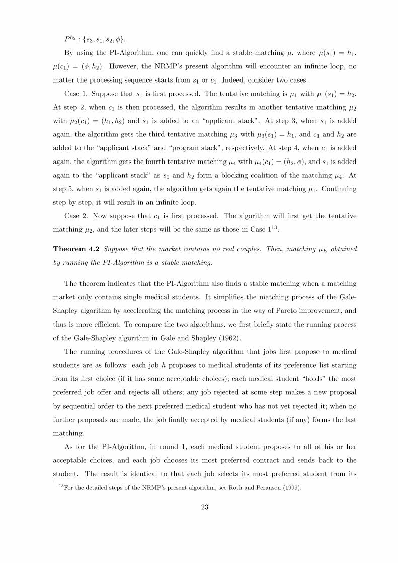
P h2 : {s3, s1, s2, ϕ}.

By using the PI-Algorithm, one can quickly find a stable matching µ, where µ(s1) = h1,

µ(c1) = (ϕ, h2). However, the NRMP’s present algorithm will encounter an infinite loop, no

matter the processing sequence starts from s1 or c1. Indeed, consider two cases.

Case 1. Suppose that s1 is first processed. The tentative matching is µ1 with µ1(s1) = h2.

At step 2, when c1 is then processed, the algorithm results in another tentative matching µ2

with µ2(c1) = (h1, h2) and s1 is added to an “applicant stack”. At step 3, when s1 is added

again, the algorithm gets the third tentative matching µ3 with µ3(s1) = h1, and c1 and h2 are

added to the “applicant stack” and “program stack”, respectively. At step 4, when c1 is added

again, the algorithm gets the fourth tentative matching µ4 with µ4(c1) = (h2, ϕ), and s1 is added

again to the “applicant stack” as s1 and h2 form a blocking coalition of the matching µ4. At

step 5, when s1 is added again, the algorithm gets again the tentative matching µ1. Continuing

step by step, it will result in an infinite loop.

Case 2. Now suppose that c1 is first processed. The algorithm will first get the tentative

matching µ2, and the later steps will be the same as those in Case 113.

Theorem 4.2 Suppose that the market contains no real couples. Then, matching µE obtained

by running the PI-Algorithm is a stable matching.

The theorem indicates that the PI-Algorithm also finds a stable matching when a matching

market only contains single medical students. It simplifies the matching process of the Gale-

Shapley algorithm by accelerating the matching process in the way of Pareto improvement, and

thus is more efficient. To compare the two algorithms, we first briefly state the running process

of the Gale-Shapley algorithm in Gale and Shapley (1962).

The running procedures of the Gale-Shapley algorithm that jobs first propose to medical

students are as follows: each job h proposes to medical students of its preference list starting

from its first choice (if it has some acceptable choices); each medical student “holds” the most

preferred job offer and rejects all others; any job rejected at some step makes a new proposal

by sequential order to the next preferred medical student who has not yet rejected it; when no

further proposals are made, the job finally accepted by medical students (if any) forms the last

matching.

As for the PI-Algorithm, in round 1, each medical student proposes to all of his or her

acceptable choices, and each job chooses its most preferred contract and sends back to the

student. The result is identical to that each job selects its most preferred student from its

13For the detailed steps of the NRMP’s present algorithm, see Roth and Peranson (1999).

23

preference list because its most preferred student must have proposed to it.14 As such, each

medical student’s choices by the two algorithms in round 1 are identical. After round 1, the PI-

Algorithm is varied from the Gale-Shapley algorithm, as medical students do not propose to those

jobs to which they prefer their current matched objects. The procedure is that each job proposes

to medical students from more preferred to less preferred ones, but not in strict sequential order.

In other words, it will skip those medical students who will reject its proposals. Compared with

the Gale-Shapley algorithm, the PI-Algorithm obviously accelerates the matching process and

improves the efficiency of algorithm. To see this, consider the following example.

Example 4.3 There are n single medical students and n+1 hospital jobs, and their preference

lists are as follows:

P s1 : {hn+1, h1, h2, · · ·, hn−1, hn, ϕ};

P s2 : {h1, h2, h3, · · ·, hn, hn+1, ϕ};

P s3 : {h2, h3, h4, · · ·, hn+1, h1, ϕ};

· · · ;

P sn : {hn−1, hn, hn+1, · · ·, hn−3, hn−2, ϕ};

P h1 : {s1, s3, s4, · · ·, sn−1, sn, s2, ϕ};

P h2 : {s2, s4, s5, · · ·, , sn, s1, s3, ϕ};

P h3 : {s3, s5, s6, · · ·, s1, s2, s4, ϕ};

· · · ;

P hn : {sn, s2, s3, · · ·, sn−2, sn−1, s1, ϕ};

P hn+1 : {s1, ϕ}.

In round 1, both the PI-Algorithm and Gale-Shapley algorithm by which the jobs first

propose to medical students get the matching µ1, where µ1(s1) = hn+1, µ1(sk) = hk, for all

2 ≤ k ≤ n. In round 2, the PI-Algorithm gets a matching µ2 with µ2(s1) = hn+1, µ2(s2) = h1,

µ2(sk) = hk, for all 3 ≤ k ≤ n. By the Gale-Shapley algorithm, however, h1 rejected by s1 in

round 1 first proposes to s3, and sequentially to s4, · · ·, sn. After rejected by those medical

students, h1 proposes to s2. s2 accepts h1’s proposal and rejects h2. The Gale-Shapley algorithm

also gets the matching µ2 after h1 sends n−1 proposals. Likewise, in round 3, the PI-Algorithm

gets a matching µ3 with µ3(s1) = hn+1, µ3(s2) = h1, µ3(s3) = h2, µ3(sk) = hk, for all 4 ≤ k ≤ n.

The Gale-Shapley algorithm also gets the matching µ3 after h2 sends n−1 proposals. By round

n, the PI-Algorithm gets the last matching µE = µn with µn(s1) = hn+1, µn(sk) = hk−1, for all

14Assume that each preference of hospital jobs is acceptable to couples; otherwise, this preference cannot

be considered effective, which does not affect any individually rational matching and can be deleted from the

preference lists of hospital jobs.

24

2 ≤ k ≤ n, and thus the process ends. However, the Gale-Shapley algorithm will not get the

last matching µE till n(n− 1)+1 rounds. Therefore, this example shows that the PI-Algorithm

significantly accelerates the matching process and thus is more efficient than the Gale-Shapley

algorithm.

For a singles market, similar to the Gale-Shapley algorithm, the PI-Algorithm may begin

with either proposals by medical students or proposals by jobs. That is, the PI-Algorithm can

begin from the set S to the set H, or similarly from the set H to the set S, and obtain stable

matchings µES and µE

HThe following theorem shows that the PI-Algorithm results in the same

matching outcomes µH and µS that are obtained by H-optimal and S-optimal15 Gale-Shapley

algorithm. Thus, the PI-Algorithm can be seen as an improvement of the Gale-Shapley algorithm

which only fits the singles market.

Theorem 4.3 For any singles market Γ = (H,S, (≻h)h∈H , (≻s)s∈S) with strict preferences,

the matchings µES and µE

H obtained by running the PI-Algorithm are the same as µH and µS

obtained by H-optimal and S-optimal Gale-Shapley algorithm, respectively.

5 Market Design

In the practice of matching markets, stable matching mechanisms play an important role.

However, in some special markets, theoretically there may not exist any stable matching mecha-

nism, such as roommate allocation problem (Gale and Shapley, 1962) and matching with couples,

etc. For matching markets with couples, if we employ semi-stable matching mechanisms, The-

orem 3.1 guarantees the existence of semi-stable matching mechanisms, and the PI-Algorithm

also ensures that semi-stable matching mechanisms are computationally feasible.

Let Γ = (H,S,C, (≻h)h∈H , (≻c)c∈C) be a couples market, andQ = {P c1 , P

c2 , ..., P

cm, P h

1 , Ph2 , ..., P

hn }

be the set of stated preference lists, one for each couple and hospital job, where each P c and P h

are couple’s and job’s preference lists.

Definition 5.1 A matching mechanism induced by the matching market Γ is a function g

whose range is the set of all possible inputs (C,H,Q) and whose output g(Q) is a matching

between C and H. If g(Q) is always stable with respect to Q, it can be called a stable matching

mechanism; if g(Q) is always semi-stable with respect to Q, it can be called a semi-stable

15H-optimal and S-optimal Gale-Shapley algorithms are respectively the algorithm that jobs first propose to

medical students and the algorithm that students first propose to jobs.

25

matching mechanism.16

For any singles market, stable mechanisms have the following properties: 1) At every stable

matching, the set of unassigned agents is the same (cf. McVitie and Wilson (1970)); 2) There

exist weakly Pareto efficient stable matchings for one side of agents (cf. Roth (1982a)); 3)

Stable mechanisms in general are not strategy-proof (cf. Dubins and Freedman (1981), Roth

(1982, 1982a, 1985), Sonmez (1997), Martinez et al. (2004), Abdulkadiroglu (2005), Hatfield and

Milgrom (2005), Klaus and Klijn (2005)). For couples markets, in general, there does not exist

a stable matching mechanism, but Theorem 3.3 guarantees the existence of a stable matching

mechanism when real couple plays reservation strategies. Also, Theorem 3.1 guarantees the

existence of a semi-stable matching mechanism.

Let µE denote a semi-stable matching obtained by the PI-Algorithm following the step-

s described in the proof of Theorem 3.1, then when g(Q) = µE , Theorem 3.1 ensures that

the mechanism is a semi-stable matching revelation mechanism, which is called PI-Algorithm

mechanism. For a matching market Γ = (H,S,C, (≻h)h∈H , (≻c)c∈C), let F be the set of all

semi-stable matchings. Define a correspondence K : F → 2F by K(µ) = {ν : ν(c) = µ(c) for

all c = (s, s′) ∈ C with s′ = ϕ}, i.e., the matched objects to real couples are the same at every

semi-stable matching of K(µ).

For marriage matching markets with strict preferences, McVitie and Wilson (1970) showed

that the set of unmatched men and women is the same at every stable matching. The following

theorem generalizes the result of McVitie and Wilson (1970), which shows that for any couples

market, the subset of semi-stable matchings K(µE) coincides with the set of all stable matchings.

Theorem 5.1 Let Γ = (H,S,C, (≻h)h∈H , (≻c)c∈C) be a couples market with strict preferences.

Suppose that µ is a semi-stable matching of Γ. Then, the set of unmatched medical students and

hospital jobs is the same at every semi-stable matching of K(µ).

The next theorem shows that there exist weakly Pareto efficient semi-stable matchings for

the side of hospital jobs.

Theorem 5.2 Let Γ = (H,S,C, (≻h)h∈H , (≻c)c∈C) be a couples market with strict preferences.

Then, the semi-stable matching µE obtained by the PI-Algorithm mechanism is weakly Pareto

efficient on K(µE) for the side of hospital jobs.

16This definition follows Roth and Sotomayor (1990). A mechanism in which players must state their preferences

is called revelation mechanism in the literature.

26

Theorem 5.2 implies that we have an optimal result for the side of hospital jobs in couples

markets. It then can be regarded as a generalization of the optimal theorem on marriage

matching markets in Roth (1982a). Also, by Theorem 4.3, for a singles market, K(µE) coincides

with the set of stable matchings, and thus we have the following corollary.

Corollary 5.1 Let Γ = (H,S, (≻h)h∈H , (≻s)s∈S) be a singles matching market with strict pref-

erences. Then the stable matching µE obtained by running the PI-Algorithm is weakly Pareto

efficient for the side of hospital jobs.

While Theorem 5.2 shows that the PI-Algorithm mechanism results in weak Pareto optimal-

ity for hospital jobs, the following theorem, however, shows that it is not strategy-proof.

Theorem 5.3 Let Γ = (H,S,C, (≻h)h∈H , (≻c)c∈C) be a couples matching market with strict

preferences. Then the PI-Algorithm mechanism is not strategy-proof on Q.

For any matching market with strict preferences Γ = (H,S,C, (≻h)h∈H , (≻c)c∈C), Theorem

3.2 shows that the set of semi-stable matchings forms a partition17, that is, F = ∪mr=1Fr, where

F is the set of all semi-stable matchings, and when m > 1, Fi ∩ Fj = ∅ for all 1 ≤ i < j ≤ m.

Indeed, here Fis denote all different K(µ)s for all µ ∈ F . Theorem 5.2 implies that there exists,

for hospital jobs, weak Pareto optimal semi-stable matching inK(µE). Let µr denote the optimal

semi-stable matching for the side of hospital jobs, then Fr = K(µr). Although Theorem 5.3 is a

negative result on strategy-proofness of the PI-Algorithm mechanism in the whole domain, the

following theorem is relatively positive.

Theorem 5.4 Let Γ = (H,S,C, (≻h)h∈H , (≻c)c∈C) be a couples market with strict preferences,

and µE be the semi-stable matching obtained by the PI-Algorithm mechanism. Suppose that

the PI-Algorithm mechanism is restricted in K(µE). Then it is a dominant strategy for every

hospital job to state its true preferences.

Since the singles market is a special case of the couples market, Theorem 5.4 generalizes the

results in Dubins and Freedman (1981) and Roth (1982a).

In the PI-Algorithm mechanism, the outcome will be a random one among µ1, µ2, · · ·, µm.

Example 5.1 below is an instance that shows the outcome is completely random. For hospital

jobs, though their welfare may be different among µ1, µ2, · · · , µm, they cannot anticipate which

µr will be obtained by the algorithm. As such, every hospital job still has incentive to tell the

truth in the PI-Algorithm mechanism. The reason is that every µr is the optimal semi-stable

17For details, see the proof of Theorem 3.2 in Appendix.

27

matching in Fr for hospital jobs, and thus, when the outcomes of mechanism are restricted in

Fr, truth-telling is a dominant strategy for every hospital job.

Example 5.1 Consider a matching market with two couples c1 = (s1, s2) and c2 = (s3, s4), one

single c3 = (s5, ϕ), and four jobs of hospitals. Their rank lists of preferences are as follows:

P c1 : {(h1, h2), (h3, h1), (h3, ϕ), (ϕ, ϕ)}; Pc2 : {(h1, h2), (ϕ, h4), (ϕ, ϕ)};

P c3 : {(h1, ϕ), (h2, ϕ), (ϕ, ϕ)};

P h1 : {s3, s2, s5, ϕ}; Ph2 : {s2, s4, s5, ϕ}; P

h3 : {s1, ϕ}; Ph4 : {s4, ϕ}.

By the PI-Algorithm mechanism, after processing PI-A1,18 we get a matching µ as follows:

µ(c1) = (h3, ϕ), µ(c2) = (ϕ, h4), µ(c3) = (ϕ, ϕ).

In the process of PI-A2, if the blocking coalition {c3, (h1, ϕ)} is stochastically obtained first,

we can get the semi-stable matching µ1 with µ1(c1) = (h3, ϕ), µ1(c2) = (ϕ, h4), µ1(c3) = (h1, ϕ).

In the process of PI-A2, if the blocking coalition {c3, (h2, ϕ)} is stochastically obtained first,

we can get the semi-stable matching µ2 with µ2(c1) = (h3, h1), µ2(c2) = (ϕ, h4), µ2(c3) = (h2, ϕ).

In the two semi-stable matchings µ1 and µ2, for couple c1, single c3, job h1 and job h2, their

welfare is changed.

6 Conclusion

This paper studies the problem of matching with couples, which can be seen as an instance

of problems with same-side complementarity. One of the typical characteristics of such problems

is that stable outcome may not exist. To overcome this defect and provide sufficient conditions

for the existence of stable matchings, we introduce the notion of semi-stable matching and

consider it as a generalized solution, which is a natural generalization of, and identical to,

the conventional stability for singles markets. It is shown that there always exists a semi-stable

matching for couples markets with strict preferences, and further the set of semi-stable matchings

can be partitioned into subsets, each of which forms a distributive lattice. When the couples

market is specialized as the singles market, semi-stable matchings of the market become stable

matchings. We also provide sufficient conditions for a semi-stable matching to be stable. If the

first preference of all real couples is one of their reservation preferences, then there exist some

stable matchings.

This result provides a perfect explanation on the puzzle of NRMP introduced by Kojima et

al. (2013). For a couples matching market, if all couples play reservation strategies, i.e., they

18For details, see the proof of Theorem 3.1 in Appendix.

28

place their reservation preferences at the top of their rank order list of preferences, which is

consistent with the stylized Facts 3 and 4 of NRMP market described by Kojima et al. (2013),

then the semi-stable matching obtained by the PI-Algorithm is a stable matching. We define the

notion of simple regular market, which simplifies the regular market presented by Kojima et al.

(2013). The stylized Facts 1 and 2 imply that NRMP market satisfies the conditions of simple

regular market. For a sequence of simple regular couples markets, when the size of market tends

to infinity, the sequence of semi-stable matchings found by the PI-Algorithm is asymptotically

stable. This also provides an interpretation for the puzzle of NRMP, which is similar to Kojima

et al. (2013).

Another remarkable contribution of the present paper is that we provide a uniform algorithm,

called the PI-Algorithm for matching with couples, which ensures finding a stable matching on

a subset of the domain that exists. Moreover, if a matching is not a semi-stable matching during

the process, the PI-Algorithm goes on processing by canceling some items from some couples’

rank lists of preferences until it converges to a semi-stable matching. In contrast to the existing

algorithms, this approach ensures finding a semi-stable matching in couples markets with strict

preferences.

Moreover, this paper studies the welfare property and incentive issues of the PI-Algorithm

mechanism from the perspective of market design. For a singles market, the results obtained by

the PI-Algorithm mechanism are the same with those of the Gale-Shapley algorithm mechanism,

while the PI-Algorithm is more efficient. For a couples market, the semi-stable matching µE

obtained by the PI-Algorithm mechanism is the optimal semi-stable matching in a subset K(µE)

of the set of all semi-stable matchings for the side of hospital jobs.

This paper also motivates further topics for research. For instance, what are the necessary

and sufficient conditions for the semi-stable matching obtained by the PI-Algorithm mechanism

to be stable? In what matching mechanisms will players have incentives to play reservation

strategies? Another important future research is to study similar issues for couples markets

with weak preferences.

29

Appendix: Proofs

Since the proofs of Theorem 3.1 and some other results need to apply Lemmas 4.1 and 4.2,

we prove them first.

Proof of Lemma 4.1: The PI-Algorithm ends when the matching of the current round

repeats the previous round. Obviously, µT−1 = µT = µE . The process of the PI-Algorithm

indicates that the preference list of each round is derived from the previous round by deleting a

part of elements. Deleting the items after µt(c) from P c(t+1) results in P c(t+1) j P c(t). X(t)

and X(t+1) are respectively derived from P c(t) and P c(t+1). As such, X(t+1) j X(t). Q.E.D.

Proof of Lemma 4.2: GivenX(t) j X(t−1) by Lemma 4.1, for any h ∈ H, if (s, h) ∈ X(t),

we have (s, h) ∈ X(t− 1). Thus, if Chh(X(t− 1)) = (s, h) and (s, h) ∈ X(t), then we must have

Chh(X(t)) = (s, h).

Consider two cases: (1) µt−1(c) = (ϕ, ϕ). Then µt(c) ≻c µt−1(c) or µt(c) = µt−1(c). (2)

µt−1(c) = (h, h′) = (ϕ, ϕ). Since (h, h′) ∈ P c(t), in the round t, we have (s, h) ∈ X(t) and

(s, h) ∈ ChH(X(t)) if h = ϕ, also (s′, h′) ∈ X(t) and (s′, h′) ∈ ChH(X(t)) if h′ = ϕ. Hence,

(h, h′) is selectable for c. Thus, we also have µt(c) ≻c µt−1(c) or µt(c) = µt−1(c). When

0 < t < T , there exists some c ∈ C such that µt(c) ≻c µt−1(c); otherwise, the PI-Algorithm ends

before round T, which contradicts the fact that it ends in round T. Q.E.D.

Proof of Theorem 3.1: We prove the theorem by finding a semi-stable matching through

the PI-Algorithm. To do so, we first prove the following two lemmas.

Lemma 6.1 Let Γ = (H,S,C, (≻h)h∈H , (≻c)c∈C) be a couples market with strict preferences,

and the matching finally obtained by the PI-Algorithm be µE. Suppose that the PI-Algorithm

ends in round T and {(s, s′), (h, h′)} is a blocking coalition of µE. Then, we have (1) whenever

h = ϕ and µE(h) = s, µE(h) = ϕ; (2) whenever h′ = ϕ and µE(h′) = s′, µE(h

′) = ϕ.

Proof: We only show statement (1), and the proof of (2) is similar. Since the PI-Algorithm

ends in round T , we have µT−1 = µT = µE by Lemma 4.1. Suppose, by way of contradiction,

that µE(h) = ϕ for h = ϕ and µE(h) = s. There are two cases to be considered.

Case 1: h′ = ϕ. Since {(s, s′), (h, ϕ)} is a blocking coalition of µE , we have s ≻h µE(h)

and (h, ϕ) ≻c µE(c). Also, since µT−1 = µT = µE , we have s ≻h µT−1(h) and (h, ϕ) ≻c

µT−1(c). Then (h, ϕ) ∈ P c(T ), and thus (s, h) ∈ X(T ). We then must have (s, h) /∈ ChH(X(T ))

30

(Otherwise, we have µT (c) ≻c (h, ϕ) or µT (c) = (h, ϕ), which contradicts the fact that (h, ϕ) ≻c

µE(c) = µT (c).). Therefore, there exists s = ϕ such that (s, h) ∈ X(T ) and (s, h) ∈ ChH(X(T )).

As such, Chh(X(T )) = (s, h). Now, if (s, h) /∈ ChC(ChH(X(T ))), then µT (h) = ϕ, contradicting

µT (h) = µE(h) = ϕ. Thus, we must have (s, h) ∈ ChC(ChH(X(T ))), and therefore µT (h) = s.

However, (s, h) /∈ ChH(X(T )), and (s, h) ∈ ChH(X(T )) implies µE(h) = µT (h) = s ≻h s, which

contradicts s ≻h µE(h). Hence, we must have µE(h) = ϕ.

Case 2: h′ = ϕ. Obviously, it implies s′ = ϕ. Since {(s, s′), (h, h′)} is a blocking coalition

of µE , (h, h′) ≻c µE(c), s ≻h µE(h) or s = µE(h), s

′ ≻h′ µE(h′) or s′ = µE(h

′). As (h, h′) ≻c

µE(c) = µT−1(c), we have (h, h′) ∈ P c(T ). Thus, (s, h) ∈ X(T ) and (s′, h′) ∈ X(T ). If

(s, h) ∈ ChH(X(T )) and (s′, h′) ∈ ChH(X(T )), then µT (c) ≻c (h, h′) or µT (c) = (h, h′), which

contradicts (h, h′) ≻c µE(c) = µT (c). Thus, either (s, h) /∈ ChH(X(T )) or (s′, h′) /∈ ChH(X(T )).

Without loss of generality, suppose (s, h) /∈ ChH(X(T )). Then, there exists s = ϕ such that

(s, h) ∈ X(T ) and (s, h) ∈ ChH(X(T )). As µT (h) = µE(h) = ϕ, µT (h) = s. (s, h) /∈ ChH(X(T ))

and (s, h) ∈ ChH(X(T )) imply µE(h) = µT (h) = s ≻h s, which contradicts s ≻h µE(h) or

s = µE(h). Hence, we must also have µE(h) = ϕ.

Thus, in either case, we have proved that whenever h = ϕ and µE(h) = s, we must have

µE(h) = ϕ. Q.E.D.

Lemma 6.2 Let Γ = (H,S,C, (≻h)h∈H , (≻c)c∈C) be a couples market with strict preferences,

and the matching finally obtained by the PI-Algorithm be µE. Suppose that for c = (s, ϕ) ∈ C,

h ∈ H, {c, (h, ϕ)} is a blocking coalition of the matching µE. Then there exists c = (s, s′)

with s′ = ϕ and h ∈ H (or c = (s, s′) with s = ϕ and h ∈ H) such that (h, h) ≻c µE(c) (or

(h, h) ≻c µE(c)).

Proof: Since the PI-Algorithm ends in round T , we have µT−1 = µT = µE by Lemma 4.1.

Also, since {c, (h, ϕ)} is a blocking coalition of µE , we have s ≻h µE(h) and (h, ϕ) ≻c µE(c).

Then (h, ϕ) ≻c µT−1(c) and (h, ϕ) ∈ P c(T ). Thus, (s, h) ∈ X(T ). We then must have (s, h) /∈

ChH(X(T )) (If so, µT (c) ≻c (h, ϕ) or µT (c) = (h, ϕ), contradicting (h, ϕ) ≻c µE(c) = µT (c).).

Thus, there is s = ϕ such that (s, h) ∈ X(T ) with (s, h) ∈ ChH(X(T )).

We show that s must be a member of real couple. Suppose not. s is then a single. Let

c1 = (s, ϕ). (s, h) ∈ ChH(X(T )) implies either µT (c1) = (h, ϕ) or µT (c1) ≻c1 (h, ϕ). However,

it is impossible to have µT (c1) = (h, ϕ) (Otherwise, we have µT (h) = s, which contradicts

µT (h) = ϕ by Lemma 6.1.). As such, we have µT−1(c1) = µT (c1) ≻c1 (h, ϕ), which implies

(h, ϕ) /∈ P c1(T ). Then, (s, h) /∈ X(T ), contradicting (s, h) ∈ X(T ). Hence, we must have s is a

member of real couple.

31

If s is the first member of a real couple, denote c = (s, s′) with s′ = ϕ. We first show

that (h, ϕ) /∈ P c(T ). Note that (s, h) ∈ ChH(X(T )) implies µT (c) ≻c (h, ϕ) or µT (c) = (h, ϕ).

We then only have µT−1(c) = µT (c) ≻c (h, ϕ), which implies (h, ϕ) /∈ P c(T ). To see this,

suppose µT (c) = (h, ϕ). Then µT (h) = s, which is impossible by noting that µT (h) = ϕ. Thus

(s, h) ∈ X(T ) implies the existence of h ∈ H such that (h, h) ∈ P c(T ), which in turn implies

(h, h) ≻c µT−1(c) = µT (c) or µT (c) = µT−1(c) = (h, h). If µT (c) = (h, h), µT (h) = s, which

contradicts µT (h) = ϕ. Therefore, (h, h) ≻c µT (c) = µE(c).

If s is the second member of a real couple, denote c = (s, s′) with s′ = s and s = ϕ. Likewise,

we can show that there exists h ∈ H such that (h, h) ≻c µE(c). Q.E.D.

With these two lemmas, we are now ready to prove the theorem. The process of finding a

semi-stable matching by the algorithm can be divided into two stages as follows:

Process PI-A1: For any couples market with strict preferences Γ = (H,S,C, (≻h)h∈H , (≻c

)c∈C), running the procedures of the PI-Algorithm described in Section IV, and supposing the

PI-Algorithm ends at round T , the matching finally obtained is µE . If µE is a semi-stable

matching, we complete the searching; otherwise we go on to the second stage.

Process PI-A2: There is a blocking coalition {c1, (h, ϕ)} of µE , where c1 = (s1, ϕ) is a single.

By Lemma 6.2, there exists c = (s, s′) with s′ = ϕ and h ∈ H (or c = (s, s′) with s = ϕ and

h ∈ H) such that (h, h) ≻c µE(c) (or (h, h) ≻c µE(c)). We only consider the case of c; the case

for c is similar. For c, deleting all of preference job pairs before µE(c) containing h from the

preference list of c, and letting P c(T +1) = P c(T ) \ {(h1, h2) ∈ H ×H : h1 = h, or, h2 = h}, the

PI-Algorithm continues on the basis of the round T . Letting the new process start from round

T + 1 to round T1, the matching obtained at the new ending is µ1E .

We first prove for any c ∈ C, µT+1(c) ≻c µT (c) or µT+1(c) = µT (c). In round T+1, obviously

X(T + 1) ⊂ X(T ). Then, for any h ∈ H, if µT (h) = s = ϕ, we have (s, h) ∈ X(T + 1), and

thus Chh(X(T + 1)) = Ch

h(X(T )) by the same argument as in the proof of Lemma 4.2. This

implies for any c ∈ C, if µT (c) = (ϕ, ϕ), µT (c) can be chosen by c at round T + 1. Therefore,

µT+1(c) ≻c µT (c) or µT+1(c) = µT (c).

We then prove there is at least one c ∈ C such that µT+1(c) ≻c µT (c). Since {c1, (h, ϕ)}

is a blocking coalition of µE , (h, ϕ) ≻c1 µE(c1) = µT (c1), (h, ϕ) ∈ P c1(T ) = P c1(T + 1), and

(s1, h) ∈ X(T + 1). Suppose Chh(X(T + 1)) = (s, h). Then s ≻h s1 or s = s1. If s = s1, then

µT+1(c1) ≻c1 (h, ϕ) or µT+1(c1) = (h, ϕ), and thus µT+1(c1) ≻c1 µT (c1); if s ≻h s1, µT (h) =

µE(h) = s1 because {c1, (h, ϕ)} is a blocking coalition of µE . Thus we have µT (h) = µE(h) = ϕ

32

by Lemma 6.1, which implies µT (s) = h. Chh(X(T +1)) = (s, h) implies (s, h) ∈ X(T +1). For

any real couple c, we have already deleted all the preference job pairs before µE(c) containing

h from the preference list of c, so s must be a single. Let c = (s, ϕ), then (s, h) ∈ X(T + 1),

which means (h, ϕ) ∈ P c(T + 1). µT (s) = h implies µT (c) = (h, ϕ), and (h, ϕ) ≻c µT (c). As

Chh(X(T + 1)) = (s, h), µT+1(c) ≻c (h, ϕ) or µT+1(c) = (h, ϕ), and µT+1(c) ≻c µT (c). Thus we

show that there exists a c ∈ C such that µT+1(c) ≻c µT (c).

By Lemma 4.2, for any c ∈ C, µ1E(c) ≻c µT+1(c) or µ

1E(c) = µT+1(c). Thus µ1

E(c) ≻c µT (c)

or µ1E(c) = µT (c), and there exists at least one c ∈ C such that µ1

E(c) ≻c µT (c). If µ1E is a

semi-stable matching, the process ends; otherwise it goes on with PI-A2. Repeating this process,

we can get matchings µ1E , µ

2E , · · ·, µ

mE until there is no blocking coalition of µm

E , {(s, ϕ), (h, ϕ)}.

The repetition will terminate because the terms of the preference lists of all c ∈ C are finite, and

for all c ∈ C, the new matching is a Pareto improvement after each repetition. As this repetition

is always in process, each single medical student will obtain his/her most preferred job, i.e., the

first item in his/her preference list. In this case, there is no blocking coalition {(s, ϕ), (h, ϕ)} of

µmE .

Obviously, the PI-Algorithm indicates that the matchings µE and µ1E , µ

2E , · · ·, µ

mE are also

individually rational. Thus we show that the matching µmE finally obtained is a semi-stable

matching of the matching market Γ = (H,S,C, (≻h)h∈H , (≻c)c∈C). Q.E.D.

Proof of Theorem 3.2: Define a correspondence K : F → 2F by

K(µ) = {ν : ν(c) = µ(c) ∀ c = (s, s′) ∈ C with s′ = ϕ},

so that all the matchings inK(µ) respectively match the same objects to real couples. Obviously,

F = ∪µ∈FK(µ) and further K(µ1) ∩ K(µ2) = ∅ for K(µ1) = K(µ2). Since such subsets are

finite, we can label them by Fi, i = 1, 2, · · ·,m. Then F = ∪mi=1Fi, and when m > 1, Fi ∩Fj = ∅

for all 1 ≤ i < j ≤ m. Thus, these subsets {Fi} constitute a partition of F . If we can show that

operations ∨C and ∧C are closed in K(µ), it is easy to verify that they meet the requirements of

idempotent law, commutative law, associative law, absorption law and distributive law, and then,

by the definition of distributive lattice,19 K(µ) constitutes a distributive lattice for operations

∨C and ∧C . Consequently, the theorem is proved.

To show that operations ∨C and ∧C are indeed closed in K(µ), i.e., λ = µ1 ∨C µ2 ∈ K(µ)

19From Birkhoff and Mac Lane (2007), a lattice is a set L of elements with two binary operations ∧ and ∨ which

are idempotent, commutative, and associative and which satisfy the absorption law. If in addition the distributive

law holds, L is called a distributive lattice.

33

and υ = µ1 ∧C µ2 ∈ K(µ), consider any c = (s, s′) ∈ C. If s′ = ϕ, by the definition of

K(µ), µ1(c) = µ2(c), thus λ(c) = υ(c) = µ1(c) = µ2(c); if s′ = ϕ, when µ1(c) = µ2(c),

λ(c) = υ(c) = µ1(c) = µ2(c); when µ1(c) ≻c µ2(c), λ(c) = µ1(c) and υ(c) = µ2(c); when

µ2(c) ≻c µ1(c), λ(c) = µ2(c) and υ(c) = µ1(c).

We now show that λ ∈ K(µ). We first prove λ is a matching. To do so, we need to show

that for any c1 ∈ C, c2 ∈ C, c1 = c2, we have (1) λ(s1) = λ(s2) for λ(s1) = ϕ and λ(s2) = ϕ, (2)

λ(s′1) = λ(s′2) for λ(s′

1) = ϕ and λ(s′2) = ϕ, (3) λ(s′1) = λ(s2) for λ(s′

1) = ϕ and λ(s2) = ϕ, and

(4) λ(s1) = λ(s′2) for λ(s1) = ϕ and λ(s′2) = ϕ.

(1) λ(s1) = λ(s2). Suppose not. There are two cases to be considered.

Case 1: s′1 = ϕ or s′2 = ϕ. Without loss of generality, suppose s′1 = ϕ.

Since λ(c1) = µ1(c1) = µ2(c1), λ(s1) = µ1(s1) = µ2(s1). If λ(c2) = µ1(c2), λ(s2) = µ1(s2),

then µ1(s1) = λ(s1) = λ(s2) = µ1(s2), which contradicts that µ1 is a matching; if λ(c2) = µ2(c2),

λ(s2) = µ2(s2), then µ2(s1) = µ2(s2), which contradicts that µ2 is a matching.

Case 2: s′1 = ϕ and s′2 = ϕ.

Case A: λ(c1) = µ1(c1) and λ(c2) = µ1(c2). It implies λ(s1) = µ1(s1) and λ(s2) = µ1(s2).

Then, µ1(s1) = µ1(s2), which contradicts that µ1 is a matching.

Case B: λ(c1) = µ2(c1) and λ(c2) = µ2(c2). It implies λ(s1) = µ2(s1) and λ(s2) = µ2(s2).

Then, µ2(s1) = µ2(s2), which contradicts that µ2 is a matching.

Case C: λ(c1) = µ1(c1) and λ(c2) = µ2(c2). It implies λ(s1) = µ1(s1) and λ(s2) = µ2(s2).

Then, µ1(s1) = µ2(s2). Let h = µ1(s1) = µ2(s2), µ1(h) = s1 and µ2(h) = s2. Since s′1 = ϕ

and s′2 = ϕ, µ1(c1) = (h, ϕ) and µ2(c2) = (h, ϕ). λ(c1) = µ1(c1) and λ(c2) = µ2(c2) respectively

imply that (h, ϕ) = µ1(c1) ≻c1 µ2(c1) and (h, ϕ) = µ2(c2) ≻c2 µ1(c2). c1 = c2 implies s1 = s2.

Therefore, if s1 ≻h s2, {c1, (h, ϕ)} is a blocking coalition of µ2, which contradicts that µ2 is a

semi-stable matching; if s2 ≻h s1, {c2, (h, ϕ)} is a blocking coalition of µ1, which contradicts

that µ1 is a semi-stable matching.

Case D: λ(c1) = µ2(c1) and λ(c2) = µ1(c2). It can also be proved by the same argument of

Case C.

Thus, by Case 1 and Case 2, if c1 = c2, we must have λ(s1) = λ(s2) for λ(s1) = ϕ and

λ(s2) = ϕ.

(2) λ(s′1) = λ(s′2). As λ(s′1) = ϕ and λ(s′2) = ϕ, we have s′1 = ϕ and s′2 = ϕ, and thus

λ(c1) = µ1(c1) = µ2(c1) and λ(c2) = µ1(c2) = µ2(c2). Since c1 = c2 implies µ1(s′

1) = µ1(s′

2),

λ(s′1) = λ(s′2).

(3) λ(s′1) = λ(s2). Since λ(s′1) = ϕ implies s′1 = ϕ, λ(c1) = µ1(c1) = µ2(c1). Also, c1 = c2

34

implies µ1(s′

1) = µ1(s2) and µ2(s′

1) = µ2(s2), but λ(s′1) = µ1(s′

1) = µ2(s′

1) and λ(s2) = µ1(s2)

or µ2(s2). Thus λ(s′

1) = λ(s2).

(4) λ(s1) = λ(s′2). The proof is similar to that of (3).

Therefore, for all c1, c2 ∈ C with c1 = c2, we have λ(s1) = λ(s2) for λ(s1) = ϕ and λ(s2) = ϕ;

λ(s′1) = λ(s′2) for λ(s′1) = ϕ and λ(s′2) = ϕ; λ(s1) = λ(s′2) for λ(s1) = ϕ and λ(s′2) = ϕ;

λ(s′1) = λ(s2) for λ(s′

1) = ϕ and λ(s2) = ϕ. Hence λ = µ1 ∨C µ2 is a matching.

Next, we prove λ = µ1 ∨C µ2 is a semi-stable matching.

Let C = C1 ∪ C2, where s′1 = ϕ for all c1 ∈ C1 and s′2 = ϕ for all c2 ∈ C2. Obviously,

C1 ∩ C2 = ∅. Let HC(µ) = {h ∈ H : there exists c2 ∈ C2 such that µ(h) = s2 or µ(h) = s′2}.

For any α ∈ K(µ), let α denote a restricted matching on (C1, [H \HC(µ)]), where α(c1) = α(c1)

for all c1 ∈ C1. Since α is a semi-stable matching, α is a stable matching. Otherwise, there exists

a blocking coalition {c1, (h1, ϕ)} of α, and obviously {c1, (h1, ϕ)} is also a blocking coalition of

α, which contradicts that α is a semi-stable matching.

For any µ1 ∈ K(µ) and µ2 ∈ K(µ), µ1 and µ2 are stable matchings on (C1, [H \ HC(µ)]).

By Conway’s lattice theorem for singles markets, λ = µ1 ∨C µ2 is also a stable matching on

(C1, [H \HC(µ)]). Therefore, λ = µ1 ∨C µ2 must be a semi-stable matching. Otherwise, there

exists a blocking coalition {c1, (h, ϕ)} of λ, where c1 ∈ C1. If h ∈ [H \ HC(µ)], {c1, (h, ϕ)}

must be a blocking coalition of λ, which contradicts that λ is a stable matching; if h ∈ HC(µ),

λ(h) = µ1(h) = µ2(h). We have λ(c1) = µ1(c1) or λ(c1) = µ2(c1), and {c1, (h, ϕ)} is a blocking

coalition of λ implies s1 ≻h λ(h) and (h, ϕ) ≻c1 λ(c1). Therefore, {c1, (h, ϕ)} is a blocking

coalition of µ1 or µ2, which contradicts that µ1 and µ2 are semi-stable matchings. Therefore,

λ = µ1 ∨C µ2 must be a semi-stable matching. Thus λ = µ1 ∨C µ2 ∈ K(µ). Similarly, we can

prove that υ = µ1 ∧C µ2 ∈ K(µ). Thus, the theorem is proved. Q.E.D.

Remark: Suppose that there are m semi-stable matchings in K(µ). Then we can easily

see that µC ≡ µ1 ∨C µ2 ∨C · · · ∨C µm and µH ≡ µ1 ∧C µ2 ∧C · · · ∧C µm are respectively the

best and worst semi-stable matching for the couples. Indeed, if c ∈ C2 or h ∈ HC(µ), then

µ(c) = µC(c) = µH(c) and µ(h) = µC(h) = µH(h) for all µ ∈ K(µ). For any α ∈ K(µ), let α

denote a restricted matching on (C1, [H \HC(µ)]), where α(c1) = α(c1) for all c1 ∈ C1. Since α

is a semi-stable matching, α is a stable matching. By the conclusion of the marriage matching

market (Knuth, 1976; Roth and Sotomayor, 1990), we have α ≥H µC and α ≤H µH . Thus,

α ≥H µC and α ≤H µH for all α ∈ K(µ). Hence, µC and µH are respectively the worst and

best semi-stable matching for the hospital jobs in K(µ).

35

Proof of Theorem 3.3: Let the matching obtained by the PI-Algorithm be µE . We show

it must be a stable matching if every real couple c’s first preference job pair (h, h′) in P c is a

reservation preference job pair of c. Obviously, the PI-Algorithm implies that µE must be an

individually rational matching. We first show µE(c) = (h, h′) for any c ∈ C with s′ = ϕ. Indeed,

at round 1 of the PI-Algorithm, the first job pair (h, h′) in P c is c’s reservation preference job

pair. If h = ϕ, then (s, h) ∈ X(T ) and (s, h) ∈ ChH(X(T )); if h′ = ϕ, then (s′, h′) ∈ X(T ) and

(s′, h′) ∈ ChH(X(T )). Thus, (h, h′) is selectable for c, and it is the first item of P c. Therefore,

µ1(c) = (h, h′). By Lemma 4.2, µE(c) ≻c µ1(c) = (h, h′) or µE(c) = µ1(c). As (h, h′) is the first

item of P c, (h, h′) ≻c µE(c) or (h, h′) = µE(c). As such, we must have µE(c) = (h, h′).

We then show that µE is stable. If not, there exists at least one blocking coalition {c1, (h1, h′

1)}

with c1 = (s1, s′

1). If s′1 = ϕ, (h1, h′

1) ≻c µE(c1), which contradicts that µE(c1) equals to the

first preference of c1. If s′1 = ϕ, then by Lemma 6.2, there exists c = (s, s′) with s′ = ϕ and

h ∈ H (or c = (s, s′) with s = ϕ and h ∈ H) such that (h1, h) ≻c µE(c) (or (h, h1) ≻c µE(c)),

which also contradicts that µE(c) (or µE(c)) equals to the first preference of c (or c). Thus, µE

must be stable. Q.E.D.

Proof of Theorem 3.4: By Theorem 3.1, for any k = 1, 2, . . ., there is a semi-stable

matching µkE in market Γk. By the definition of semi-stable matching, any blocking coalition

{c, (h, h′)} of µkE contains a real couple c = (s, s′), and (h, h′) must be its effective prefer-

ence. By Condition 2 for simple regularity, the number of blocking coalitions of µkE must be

less than mk · γ(lnnk)λ. For the null matching µ0, the number of its blocking coalitions is

N =∑

c∈Ck lc. By Condition 3 for simple regularity, we have N ≥ nk. Thus, the instability

degree is θ(µkE) = m/N ≤ mk · γ(lnnk)

λ/nk. By Condition 1 for simple regularity, mk ≤ nk1−ϵ,

and we have θ(µkE) ≤ γ(lnnk)

λ/nkϵ. Thus limnk→∞ θ(µk

E) = 0, that is, as nk tends to infinity,

the sequence of instability degree {θ(µkE)}

∞

k=1tends to zero. Therefore, the matching sequence

{µkE}

∞

k=1is asymptotically stable, that is, {Γk}∞k=1

is asymptotically stable. Q.E.D.

Proof of Theorem 3.5: Let the semi-stable matching obtained by the algorithm described

in Section IV be µE . We need to show that µE is a stable matching. It is clear that the PI-

Algorithm indicates that µE must be individually rational.

We first show that for any c ∈ C with s′ = ϕ, µE(c) = (h, h′). Indeed, at round 1 of the

PI-Algorithm, (h, h′) is c’s reservation preference job pair, which implies that if h = ϕ, then

36

(s, h) ∈ X(T ) and (s, h) ∈ ChH(X(T )); if h′ = ϕ, then (s′, h′) ∈ X(T ) and (s′, h′) ∈ ChH(X(T )).

Thus, (h, h′) is selectable for c at round 1, and µ1(c) ≻c (h, h′) or µ1(c) = (h, h′).

We now show µ1(c) = (h, h′). Suppose, by way of contradiction, that µ1(c) = (h, h′).

Then we must have µ1(c) = (h, h′

) ≻c (h, h′). Thus, (h, ϕ) = (ϕ, ϕ) or (h′, ϕ) = (ϕ, ϕ) implies

that it is not only a reservation preference term but also the first preference term of a single.

Therefore, if h = ϕ, there exists c = (s, ϕ) such that (s, h) ∈ X(T ) and (s, h) ∈ ChH(X(T )), and

µ1(c) = (h, ϕ) because (h, ϕ) is the first preference term of c; if h′

= ϕ, there exists c = (s, ϕ)

such that (s, h′

) ∈ X(T ) and (s, h′

) ∈ ChH(X(T )), and µ1(c) = (h′

, ϕ) because (h′

, ϕ) is the

first preference term of c. This contradicts µ1(c) = (h, h′

). Hence µ1(c) = (h, h′).

For any preference (h, h′

) of c before (h, h′), if h = ϕ, there exists c = (s, ϕ) such that

µ1(c) = (h, ϕ). The process of the PI-Algorithm for finding semi-stable matching µE implies

that µE(c) ≻c µ1(c) for any c ∈ C. However, since (h, ϕ) is the first preference term of c,

µE(c) = (h, ϕ). Likewise, if h′

= ϕ, there exists c = (s, ϕ) such that µE(c) = (h′

, ϕ). Thus

µE(c) = µ1(c) = (h, h′) by noting that it cannot be matched to an object which is better than

(h, h′) for c.

Now, if the semi-stable matching µE is not a stable matching, there exists at least one

blocking coalition {c1, (h1, h′

1)} with s′1 = ϕ. As such, we have (h1, h′

1) ≻c µE(c1). Moreover,

s1 ≻h1µE(h1) if h1 = ϕ, and s′1 ≻h′

1µE(h

′

1) if h′1 = ϕ. However, as shown above, if h1 = ϕ,

then there exists c1 = (s1, ϕ) such that µE(c1) = (h1, ϕ), which contradicts s1 ≻h1µE(h1) = s1

by noting that (h1, ϕ) is a reservation preference term of c1 implies that s1 ≻h1s1; if h

′

1 = ϕ,

then there exists c1 = (s1, ϕ) such that µ1(c1) = (h′1, ϕ), which contradicts s′1 ≻h′

1µE(h

′

1) = s1

by noting that (h′1, ϕ) is a reservation preference term of c1 implies that s1 ≻h′

1s′1. Thus µE

must be a stable matching. Q.E.D.

Proof of Theorem 4.1: It is clear that the PI-Algorithm implies the matching µE is

an individually rational matching. Suppose, by way of contradiction, that µE is not a stable

matching. Then there exists a blocking coalition {(s, s′), (h, h′)} with µE(h) = ϕ and µE(h′) = ϕ.

However, by Lemma 6.1, µE(h) = ϕ = µE(h′) when h = ϕ, µE(h) = s, h′ = ϕ, µE(h

′) = s′.

As such, µE(h) = ϕ and µE(h′) = ϕ imply µE(h) = s and µE(h

′) = s′, which contradicts that

{(s, s′), (h, h′)} is a blocking coalition of µE . Q.E.D.

Proof of Theorem 4.2: Again, the PI-Algorithm clearly implies that the matching µE

must be an individually rational matching. Suppose that µE is not a stable matching, there

37

exists at least one blocking coalition {(s, s′), (h, ϕ)} of µE . By Lemma 6.2, there exists c = (s, s′)

with s′ = ϕ and h ∈ H (or c = (s, s′) with s = ϕ and h ∈ H) such that (h, h) ≻c µE(c) (or

(h, h) ≻c µE(c)), which contradicts that Γ has no real couples. Q.E.D.

Proof of Theorem 4.3: For any singles market Γ = (H,S,C, (≻h)h∈H , (≻c)c∈C), the

subset K(µES ) of the set of semi-stable matchings is identical to the set of stable matchings. By

Theorem 5.2, the matching µES is the optimal stable matching for the side of hospital jobs. The

optimal theorem of marriage matching markets (Roth, 1982a) implies that µH is the optimal

stable matching for the side of hospital jobs. Since the optimal matching is unique, we have

µES = µH . For any singles market, µE

H and µES are logically symmetrical. Likewise, we have

µEH = µS . Q.E.D.

Proof of Theorem 5.1: Since matched object of each real couple is the same for all semi-

stable matchings in K(µ), the set of unmatched real couples is the same at every semi-stable

matching in K(µ). After excluding all real couples and their matched objects, the semi-stable

matching is actually a stable matching for singles and all remaining jobs of hospitals. By M-

cVitie and Wilson theorem, the set of unmatched single medical students and remaining jobs of

hospitals is the same for every stable matching. Q.E.D.

Proof of Theorem 5.2: To prove the theorem, we need the following lemma:

Lemma 6.3 Let Γ = (H,S,C, (≻h)h∈H , (≻c)c∈C) be a couples market with strict preferences,

and the outcome obtained by the PI-Algorithm mechanism be µE. Suppose that for every µ ∈

K(µE), there exists h ∈ H such that s = µ(h) ≻h µE(h). Then s must be a single, h1 = µE(s) =

ϕ, and µ(h1) ≻h1µE(h1).

Proof: Since µ and µE are semi-stable matchings, they are both individually rational, and

µE(h) ≻h ϕ or µE(h) = ϕ. Since s = µ(h) ≻h µE(h), s = µ(h) ≻h ϕ, which implies µ(s) = h =

ϕ. By Theorem 5.1, the set of unmatched medical students is the same for every semi-stable

matching in K(µE), which implies that the set of matched medical students is also the same

for every semi-stable matching in K(µE). Thus, h1 = µE(µ(h)) = µE(s) = ϕ, s = µE(h1).

Let s1 = µ(h1), then µ(h) ≻h µE(h) implies s = µ(h) = µE(h). Thus h1 = µE(s) = h, and

s1 = µ(h1) = µ(h) = s. We show s must be a single. If not, s is a member of a real couple c,

then µ(c) = µE(c) because µ ∈ K(µE). Thus h = µ(s) = µE(s) = h1, contradicting h1 = h.

Next, we show that h1 ≻s h = µ(s).

38

Since µ and µE are individually rational and h1 = ϕ = h, we have h1 = µE(s) ≻s ϕ

and h = µ(s) ≻s ϕ. Thus, at step 1 of round 1 in the process of the PI-Algorithm, we have

(s, h) ∈ X(1) and (s, h1) ∈ X(1). Noting that the PI-Algorithm ends at round T and letting

s = µE(h), we have (s, h) ∈ X(T ) and (s, h) ∈ ChH(X(T )). Since s = µ(h) ≻h µE(h) = s,

we have (s, h) /∈ X(T ); otherwise, it contradicts (s, h) ∈ ChH(X(T )). Since (s, h) /∈ X(T ),

by Lemma 4.1 ,we have h1 = µE(s) = µT−1(s) ≻s h, where µT−1 is the temporary matching

obtained at round T-1.

If s ≻h1s1 = µ(h1), as h1 ≻s h = µ(s), {(s, ϕ), (h1, ϕ)} constitutes a blocking coalition of

matching µ, which contradicts that µ is a semi-stable matching. Hence µ(h1) = s1 ≻h1s =

µE(h1). Q.E.D.

Now we begin to prove the theorem. Suppose, by way of contradiction, that µE is not weakly

Pareto efficient on K(µE) for the side of hospital jobs, then there exists a matching µ ∈ K(µE)

such that for all h ∈ H, µ(h) ≻h µE(h) or µ(h) = µE(h), and there exists an h ∈ H such

that µ(h) ≻h µE(h) . Let s1 = µ(h) and h1 = µE(s1). By Lemma 6.3, s1 must be a single,

h1 = ϕ and µ(h1) ≻h1µE(h1). Repeatedly applying Lemma 6.3, we can obtain two sequences,

one is the sequence of medical students {s1, s2, · · · }, and the other is the sequence of hospital

jobs {h1, h2, . . . , }, where sk+1 = µ(hk) and hk = µE(sk) for any k > 0. Due to the limited

number of medical students, there exists the least k and r such that sk+r = sk. Thus k = 1;

otherwise hk+r−1 = µ(sk) = hk−1 and sk+r−1 = µE(hk−1) = sk−1, which contradicts that k is

the least. Therefore, k = 1, that is, s1 = sr+1 and h0 = hr. It is easy to deduce that sl = sl+r

and hl = hl+r for any l > 0. Thus, we obtain twin circulating sequences: the sequence of

medical students {s1, s2, · · · , sr} and the sequence of hospital jobs {h1, h2, · · · , hr}, such that

sk+1 = µ(hk), hk = µE(sk) and sk+1 ≻hksk for any k > 0. We now show that there are no such

twin circulating sequences. As a result, the theorem is proved.

Denote by H ⊆ H the set of all jobs satisfying the condition µ(h) ≻h µE(h). We consider

two cases.

Case 1: H = {h1, h2, · · · , hr}. For any 2 ≤ k ≤ r+1, µ and µE are both semi-stable match-

ings, which implies that they are both individually rational, and thus hk = µE(sk) ≻sk ϕ and

hk−1 = µE(sk−1) ≻sk−1ϕ. At the step 1 of round 1 in the process of the PI-Algorithm, (sk, hk) ∈

X(1) and (sk−1, hk−1) ∈ X(1). Suppose the PI-Algorithm ends at round T and gives the tem-

porary matching µt at round t, since hk−1 = µE(sk−1) = µT (sk−1), we have (sk−1, hk−1) ∈

X(T ) and (sk−1, hk−1) ∈ ChH(X(T )). Also, since sk = µ(hk−1) ≻hk−1µE(hk−1) = sk−1,

39

(sk, hk−1) /∈ X(T ) (Otherwise, it contradicts (sk−1, hk−1) ∈ ChH(X(T )).). Thus, (sk, hk−1) ∈

X(1) and (sk, hk−1) /∈ X(T ) imply that there exists 1 < tk < T such that (sk, hk−1) ∈ X(tk)

and (sk, hk−1) /∈ X(tk + 1). Without loss of generality, suppose tk is the least one. Then

h ≡ µtk(sk) ≻sk hk−1 = µ(sk). Thus we must have h /∈ H. Indeed, suppose not. Then

µtk(sk) = h = hj = µE(sj). As such, (sj , hj) ∈ ChH(X(tk)) and (sj+1, hj) /∈ X(tk) by noting

that sj+1 = µ(hj) ≻hjµE(hj) = sj . Also, (sj+1, hj) ∈ X(1) by noting that sj+1 ≻hj

sj ≻hjϕ.

Thus, there exists tj such that (sj+1, hj) ∈ X(tj) and (sj+1, hj) ∈ X(tj + 1). We then have

tj < tk because (sj+1, hj) ∈ X(tj) and (sj+1, hj) ∈ X(tk), which contradicts the hypothesis that

tk is the least. So h /∈ H.

Let s = µ(h). Then s = ϕ. Suppose not. Since h = µtk(sk) ≻sk hk−1 = µ(sk), sk ≻h ϕ and

sk is a single, {(sk, ϕ), (h, ϕ)} forms a blocking coalition of matching µ, which contradicts the

fact that µ is a semi-stable matching. So we must have s = ϕ. Then, by Theorem 5.1, we have

s ≡ µE(h) = ϕ. Therefore, s, s and sk are all acceptable medical students for h. Since h has

chosen sk before the final matching s, we have sk ≻h s. If s ≻h s or s = s, then sk ≻h s = µ(h).

Consequently, {(sk, ϕ), (h, ϕ)} is a blocking coalition of the matching µ, which contradicts that

µ is a semi-stable matching. Thus s ≻h s, that is, µ(h) ≻h µE(h), and h ∈ H. However, this

contradicts h /∈ H. Hence µE must be an optimal semi-stable matching in K(µE) for the side

of hospital jobs when H = {h1, h2, · · · , hr}.

Case 2: H = {h1, h2, · · ·, hr}. By repeating the above proof, we can obtain the circulat-

ing sequence of medical students {s1, s2, · · · , sr} and the circulating sequence of hospital jobs

{h1, h2, · · · , hr} such that sk+1 = µ(hk), hk = µE(sk) and sk+1 ≻hksk for any k > 0. The pre-

requisite of twin circulating sequences is that there exists at least one h /∈ {h1, h2, · · · , hr} such

that µ(h) ≻h µE(h). Applying Lemma 6.3 again, we obtain another twin circulating sequences

satisfying the same conditions. By repeating the proving process in Case 1, the prerequisite of

this new twin circulating sequences is another new twin circulating sequences, and it similarly

shows that these different twin circulating sequences do not intersect with each other. The same

argument can be repeated endlessly, thus we can obtain infinite twin circulating sequences. S-

ince H is a finite set, all these twin circulating sequences are bound to constitute a causal circle,

that is, the prerequisite of the first twin circulating sequences is the existence of the second twin

circulating sequences, and the prerequisite of the second twin circulating sequences is the exis-

tence of the third twin circulating sequences, and so on, which leads to a contradiction. Thus,

µE must be a weakly Pareto efficient semi-stable matching in K(µE) for the side of hospital jobs

when H = {h1, h2, · · · , hr}. Q.E.D.

40

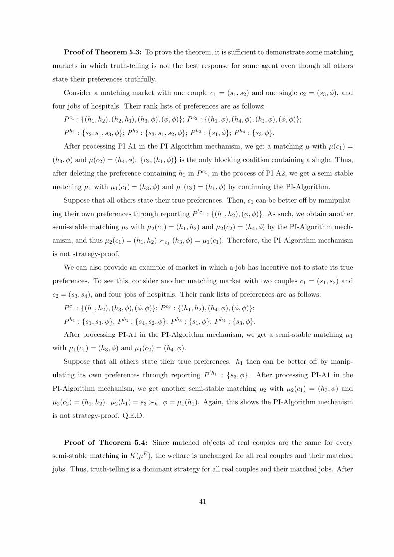
Proof of Theorem 5.3: To prove the theorem, it is sufficient to demonstrate some matching

markets in which truth-telling is not the best response for some agent even though all others

state their preferences truthfully.

Consider a matching market with one couple c1 = (s1, s2) and one single c2 = (s3, ϕ), and

four jobs of hospitals. Their rank lists of preferences are as follows:

P c1 : {(h1, h2), (h2, h1), (h3, ϕ), (ϕ, ϕ)}; Pc2 : {(h1, ϕ), (h4, ϕ), (h2, ϕ), (ϕ, ϕ)};

P h1 : {s2, s1, s3, ϕ}; Ph2 : {s3, s1, s2, ϕ}; P

h3 : {s1, ϕ}; Ph4 : {s3, ϕ}.

After processing PI-A1 in the PI-Algorithm mechanism, we get a matching µ with µ(c1) =

(h3, ϕ) and µ(c2) = (h4, ϕ). {c2, (h1, ϕ)} is the only blocking coalition containing a single. Thus,

after deleting the preference containing h1 in P c1 , in the process of PI-A2, we get a semi-stable

matching µ1 with µ1(c1) = (h3, ϕ) and µ1(c2) = (h1, ϕ) by continuing the PI-Algorithm.

Suppose that all others state their true preferences. Then, c1 can be better off by manipulat-

ing their own preferences through reporting P′c1 : {(h1, h2), (ϕ, ϕ)}. As such, we obtain another

semi-stable matching µ2 with µ2(c1) = (h1, h2) and µ2(c2) = (h4, ϕ) by the PI-Algorithm mech-

anism, and thus µ2(c1) = (h1, h2) ≻c1 (h3, ϕ) = µ1(c1). Therefore, the PI-Algorithm mechanism

is not strategy-proof.

We can also provide an example of market in which a job has incentive not to state its true

preferences. To see this, consider another matching market with two couples c1 = (s1, s2) and

c2 = (s3, s4), and four jobs of hospitals. Their rank lists of preferences are as follows:

P c1 : {(h1, h2), (h3, ϕ), (ϕ, ϕ)}; Pc2 : {(h1, h2), (h4, ϕ), (ϕ, ϕ)};

P h1 : {s1, s3, ϕ}; Ph2 : {s4, s2, ϕ}; P

h3 : {s1, ϕ}; Ph4 : {s3, ϕ}.

After processing PI-A1 in the PI-Algorithm mechanism, we get a semi-stable matching µ1

with µ1(c1) = (h3, ϕ) and µ1(c2) = (h4, ϕ).

Suppose that all others state their true preferences. h1 then can be better off by manip-

ulating its own preferences through reporting P′h1 : {s3, ϕ}. After processing PI-A1 in the

PI-Algorithm mechanism, we get another semi-stable matching µ2 with µ2(c1) = (h3, ϕ) and

µ2(c2) = (h1, h2). µ2(h1) = s3 ≻h1ϕ = µ1(h1). Again, this shows the PI-Algorithm mechanism

is not strategy-proof. Q.E.D.

Proof of Theorem 5.4: Since matched objects of real couples are the same for every

semi-stable matching in K(µE), the welfare is unchanged for all real couples and their matched

jobs. Thus, truth-telling is a dominant strategy for all real couples and their matched jobs. After

41

excluding all real couples and their matched objects, the semi-stable matching is actually a stable

matching for all singles and remaining hospital jobs. By Theorem 4.3, for any matching market

containing only singles with strict preferences, the matching obtained by the PI-Algorithm is

identical to µH which is obtained by jobs optimal Gale-Shapley algorithm. By the dominant

strategy theorem on marriage matching markets in Dubins and Freedman (1981) and Roth

(1982a), telling the truth is a dominant strategy for each remaining job of hospitals. Q.E.D.

42

References

[1] Abdulkadiroglu, Atila [2005]: “College Admission with Affirmative Action,” International

Journal of Game Theory 33, 535-549.

[2] Aldershof, Brian and Olivia M. Carducci [1996]: “Stable Matchings with Couples ” Discrete

Applied Mathematics (68)1-2, 203-207.

[3] Birkhoff, Garrett and Saunders Mac Lane [2007]: “A Survey of Modern Algebra,” A K

Peters, Ltd. And Posts and Telecom Press, China.

[4] Crawford, Vincent P., and Elsie Marie Knoer [1981]: “Job Matching with Heterogeneous

Firms and Workers,” Econometrica 49(2):437-50.

[5] Dubins, L.E., Freedman, D.A. [1981]: “Machiavelli and the Gale-Shapley algorithm,”

American Mathematical Monthly 88, 485-494.

[6] Hatfield J. W. and P. R. Milgrom [2005]: “Matching with Contracts,” American Economic

Review 95, 913-935.

[7] Gale David and Lloyd S. Shapley [1962]: “College Admissions and the Stability of Mar-

riage,” American Mathematical Monthly 69, 9-15.

[8] Kelso, Alexander S., Jr., and Vincent P. Crawford [1982]: “Job Matching, Coalition For-

mation, and Gross Substitutes,” Econometrica 50(6):1483-1504.

[9] Klaus Bettina and Flip Klijn [2005]: “Stable Matching and Preferences of Couples,” Journal

of Economic Theory 121, 75-106.

[10] Klijn F. and J. Masso [2003]: “Weak Stability and a Bargaining Set for the Marriage

Model,” Games and Economic Behavior 42, 91-100.

[11] Knuth, Donald E. [1976]: “Mariages Stables, Montreal,” Les Presses de l’Universite de

Montreal.

[12] Kojima F. and P. A. Pathak [2009]: “Incentives and Stability in Large Two-sided Matching

Markets,” American Economic Review 99, 608-627.

[13] Kojima F. P. A. Pathak and A. V. Roth [2013]: “Matching with Couples: Stability and

Incentives in Large Markets,” Quarterly Journal of Economics 128, 1585-1632.

43

[14] Martinez, Ruth, Masso, Jordi, Neme, Alejandro, Ovideo, Jorge [2004]: “On group strategy-

proof mechanisms for many-to-one matching model,” International Journal of Game Theory

33, 115-128.

[15] McVitie, D. G. and L. B. Wilson [1970]: “Stable Marriage Assignments for Unequal Sets,”

BIT, 10, 295-309.

[16] Ostrovsky Michael [2008]: “Stability in Supply Chain Networks,” American Economic Re-

view 98, 897-923.

[17] Ronn Eytan [1990]: “NP-complete stable matching problems,” Journal of Algorithms 11,

2, June, 285-304.

[18] Roth Alvin E. [1982]: “The economics of matching: stability and incentives,” Mathematics

of Operations Research 7, 617-628.

[19] Roth Alvin E. [1982a]: “The Economics of Matching: Stability and Incentives,” Mathe-

matics of Operations Research Vol. 7, 617-628.

[20] Roth Alvin E. [1984]: “The Evolution of the Labor Market for Medical Interns and Resi-

dents: A Case Study in Game Theory,” Journal of Political Economy 92, 991-1016.

[21] Roth Alvin E. [1985]: “The College Admissions Problem is not Equivalent to the Marriage

Problem,” Journal of Economic Theory 36, 277-288.

[22] Roth Alvin E. [2008]: “Deferred Acceptance Algorithms: History, Theory, Practice, and

Open Questions,” International Journal of Game Theory 36, 537-569.

[23] Roth A. E. and E. Peranson [1999]: “The Redesign of the Matching Market for American

Physicians: Some Engineering Aspects of Economic Design,” American Economic Review

89, 748-780.

[24] Roth A. E. and M. A. O. Sotomayor [1990]: “Two-Sided Matching: A Study in Game

Theoretic Modeling and Analysis,” Econometric Society Monograph Series, Cambridge U-

niversity Press New York, 1990.

[25] Roth A. E. and Vande Vate John H. [1990]: “Random Paths to Stability in Two-Sided

Matching,” Econometrica 58, 1475-1480.

[26] Sonmez, Tayfun [1997]: “Manipulation via Capacities in Two-Sided Matching Markets,”

Journal of Economic Theory 77, 197-204.

44

[27] Ning Sun and Zaifu Yang [2006]: “Equilibria and Indivisibilities: Gross Substitutes and

Complements,” Econometrica 74, 1385-1402.

[28] Ning Sun and Zaifu Yang [2009]: “Double-Track Adjustment Process for Discrete Markets

with Substitutes and Complements,” Econometrica 77, 933-952.

[29] Zhou L. [1994]: “A New Bargaining Set of an N-person Game and Endogenous Coalition

Formation,” Games and Economic Behavior 6, 512-526.

45